HOLLOW CYLINDER DYNAMIC PRESSURIZATION AND RADIAL …

HOLLOW CYLINDER DYNAMIC PRESSURIZATION AND

RADIAL FLOW THROUGH PERMEABILITY TESTS FOR

CEMENTITIOUS MATERIALS

A Thesis

by

CHRISTOPHER ANDREW JONES

Submitted to the Office of Graduate Studies of

Texas A&M University

in partial fulfillment of the requirements for the degree of

MASTER OF SCIENCE

August 2008

Major Subject: Civil Engineering

HOLLOW CYLINDER DYNAMIC PRESSURIZATION AND

RADIAL FLOW THROUGH PERMEABILITY TESTS FOR

CEMENTITIOUS MATERIALS

A Thesis

by

CHRISTOPHER ANDREW JONES

Submitted to the Office of Graduate Studies of

Texas A&M University

in partial fulfillment of the requirements for the degree of

MASTER OF SCIENCE

Approved by:

Chair of Committee, Zachary C. Grasley

Committee Members, K. Ted Hartwig

Robert L. Lytton

Head of Department, David Rosowsky

August 2008

Major Subject: Civil Engineering

iii

ABSTRACT

Hollow Cylinder Dynamic Pressurization and Radial Flow Through Permeability Tests

for Cementitious Materials. (August 2008)

Christopher Andrew Jones, B.S., Texas A&M University; B.A., Southwestern

University

Chair of Advisory Committee: Dr. Zachary C. Grasley

Saturated permeability is likely a good method for characterizing the susceptibility of

portland cement concrete to various forms of degradation; although no widely accepted

test exists to measure this property. The hollow cylinder dynamic pressurization test is

a potential solution for measuring concrete permeability. The hollow cylinder dynamic

pressurization (HDP) test is compared with the radial flow through (RFT) test and the

solid cylinder dynamic pressurization (SDP) test to assess the accuracy and reliability of

the HDP test.

The three test methods, mentioned above, were used to measure the permeability of

Vycor glass and portland cement paste and the results of the HDP test were compared

with the results from the SDP and RFT tests. When the HDP and RFT test results were

compared, the measured difference between the mean values of the two tests was 40%

for Vycor glass and 47% for cement paste. When the HDP and SDP tests results were

compared, the measured difference with Vycor glass was 53%. The cement paste

iv

permeability values could not be compared in the same manner since they were tested at

various ages to show the time dependency of permeability in cement paste.

The results suggest good correlation between the HDP test and both the SDP and RFT

tests. Furthermore, good repeatability was shown with low coefficients of variation in

all test permutations. Both of these factors suggest that the new HDP test is a valid tool

for measuring the permeability of concrete materials.

v

DEDICATION

To Lauren and the girls.

vi

ACKNOWLEDGEMENTS

I would like to thank my committee chair, Dr. Grasley, for teaching me and for helping

me to gain a more complete understanding of the materials field. His help and guidance

has been invaluable in this process. Furthermore, I appreciate the sacrifice of my

committee members who supported me through the revision process.

Thanks also go to my friends and coworkers without whom I would surely have gone

crazy. I also want to extend my gratitude to the Ready Mix Concrete Foundation, which

provided funding and support for my work. Additionally, the Transportation Scholars

Program, Jones and Carter Inc., and the Chemical Lime Company have all financially

supported my educational endeavors.

Finally, thanks to my mother and father for their encouragement and to my wife for all

her patience and love.

vii

NOMENCLATURE

w/c water to cement

HDP hollow dynamic pressurization

SDP solid dynamic pressurization

RFT radial flow through

viii

TABLE OF CONTENTS

Page

ABSTRACT ..................................................................................................................... iii

DEDICATION ................................................................................................................... v

ACKNOWLEDGEMENTS .............................................................................................. vi

NOMENCLATURE .........................................................................................................vii

TABLE OF CONTENTS ............................................................................................... viii

LIST OF FIGURES ............................................................................................................ x

LIST OF TABLES ...........................................................................................................xii

1 INTRODUCTION ...................................................................................................... 1

1.1 Problem Statement ............................................................................................... 1

1.2 Scope ................................................................................................................... 3

1.3 Thesis Outline ...................................................................................................... 3

2 CURRENT STATE OF PERMEABILITY MEASUREMENTS .............................. 5

2.1 Direct Permeability Measurement ....................................................................... 5

2.2 Non Direct Permeability Measurement ............................................................... 6

3 DEVELOPMENT OF A NEW PERMEABILITY TESTING APPARATUS .......... 9

3.1 General Apparatus Requirements ........................................................................ 9

3.2 Radial Flow Through Apparatus ....................................................................... 10 3.3 Hollow Dynamic Pressurization Apparatus ...................................................... 13

3.4 Solid Dynamic Pressurization Apparatus .......................................................... 15

4 TEST THEORY ....................................................................................................... 17

4.1 Radial Flow Through ......................................................................................... 17 4.2 Hollow Dynamic Pressurization ........................................................................ 19

5 EXPERIMENTAL TECHNIQUES ......................................................................... 30

ix

Page

5.1 Specimen Materials and Preparation ................................................................. 30

5.2 Porosity Determination ...................................................................................... 33 5.3 Fluid Viscosity Determination ........................................................................... 35 5.4 Fluid Bulk Modulus Determination ................................................................... 36 5.5 Testing Program ................................................................................................ 37

6 RESULTS AND DISCUSSION .............................................................................. 39

6.1 Vycor ................................................................................................................. 39

6.1.1 Hollow Dynamic Pressurization Versus Radial Flow Through ................. 40

6.1.2 Hollow Dynamic Pressurization Versus Solid Dynamic Pressurization .... 43 6.2 Cementitious Materials ...................................................................................... 45

6.2.1 Hollow Dynamic Pressurization Versus Radial Flow Through ................. 46 6.2.2 Hollow Dynamic Pressurization Versus Solid Dynamic Pressurization .... 49

7 SUMMARY ............................................................................................................. 51

REFERENCES ................................................................................................................. 52

APPENDIX A. VYCOR PLOTS ..................................................................................... 55

APPENDIX B. CEMENTITIOUS MATERIALS PLOTS .............................................. 95

VITA .............................................................................................................................. 130

x

LIST OF FIGURES

Page

Figure 1: The radial flow through (RFT) apparatus that pressurizes the outer

surface of a sample and monitors the fluid volume that flows

through as a function of time. ........................................................................... 12

Figure 2: The hollow dynamic pressurization (HDP) apparatus consists of a

pressure vessel and a non-contact LVDT system which measures

the axial deformation of the specimen. ............................................................. 14

Figure 3: The solid dynamic pressurization (SDP) apparatus consists of a

pressure vessel and a non-contact LVDT which measures the axial

contraction of the specimen. ............................................................................. 16

Figure 4. Comparison of relaxation functions for solid and hollow cylinders.

Note that the early behavior (θ < 0.01) is comparable for both

functions. In this case Ro/Ri is equal to 3.937 which corresponds to

a 10.16 cm (4 inch) diameter cylinder with a 2.54 cm (1 inch)

diameter hole. ................................................................................................... 24

Figure 5: The fit parameter m is determined by curve fitting several different

radius ratios. ..................................................................................................... 26

Figure 6: The fit parameter n is determined by fitting the results of various

radius ratios. ..................................................................................................... 27

Figure 7. Approximation of the relaxation function Ω(θ) using eq. (30). The

discrete points are numerically inverted data for Ω(θ) while the

solid line is the approximate function. The function is evaluated

using properties typical of concrete: β = 1/2, b = 2/3, λ = 1/4. ........................ 28

Figure 8: The hollow Vycor and cement paste specimens are sealed at each

end with special caps, secured by a two part marine epoxy. ............................ 33

Figure 9: The porosity of the cement paste specimens as a function of age. .................... 35

Figure 10: Typical hollow dynamic pressurization strain data shown on time

and log-time axes. The log-time axis more clearly shows when the

specimen has fully relaxed. .............................................................................. 40

xi

Page

Figure 11: The results of the hollow dynamic pressurization test and the solid

dynamic pressurization tests shown as a function of age. For

comparison purposes the results from some other studies are

included. ........................................................................................................... 50

xii

LIST OF TABLES

Page

Table 1: The concrete mix design used in the testing is representative of a

typical driveway or sidewalk mix. .................................................................... 31

Table 2: Since the Vycor tubes have a thin wall thickness, fluids with higher

viscosities than water were used to slow the Hollow Dynamic

Pressurization test. ............................................................................................ 36

Table 3: The bulk modulus values for the testing fluid are used in calculating

the permeability for each specimen with the dynamic pressurization

methods. ............................................................................................................ 37

Table 4: The tabulated results of the Vycor permeability testing show good

agreement between the various test permutations of fluid and test

method. ............................................................................................................. 41

Table 5: The measured Vycor permeability and associated statistical quantities

measured with various fluids. ........................................................................... 44

Table 6: The permeability results from the 0.6 w/c paste show good

correlation between the HDP and the radial flow through

techniques. ........................................................................................................ 47

1

1 INTRODUCTION

1.1 PROBLEM STATEMENT

Though generally considered a very durable material, portland cement concrete has

shown significant susceptibility to various forms of chemical and physical damage

which reduce the service life of many concrete structures. Not surprisingly, the problem

of concrete durability has a significant monetary impact on society. Various studies have

tried to quantify the impact of these mechanisms with most estimates ranging in the

billions of dollars per year in the United States alone [1] where much of the cost is borne

by the taxpaying public. Corrosion of reinforcing steel is the most widespread form of

concrete deterioration which is directly related to the ability of external chloride ions

(usually in solution) to move into the pore network and react with the reinforcement [2].

Many if not all, of these degradation mechanisms are tied to moisture within the

concrete. Alkali-aggregate reactivity [3], sulfate attack [4], corrosion of reinforcing steel

[5], and freeze-thaw damage [2] are examples of real-world problems that are related to

moisture intrusion into the pore network of the concrete. It has long been theorized that

there is a fundamental link between concrete permeability and its durability [6] though

real scientific data to support this claim is lacking. In many cases the actual mechanism

of ion or moisture movement within the material is not saturated flow, but vapor

____________

This thesis follows the style of Cement and Concrete Research.

2

diffusion or capillary sorption [7]. Nonetheless, the interplay of the various transport

mechanisms is far from being fully understood, and saturated permeability provides a

consistent and reproducible measurement of the penetrability of the concrete. In theory

establishing the connection between saturated permeability and the various forms of

concrete degradation would be a rather simple experiment, but due to the lack of a

consistent and repeatable concrete permeability test the relationship between the various

degradation mechanisms and permeability is not clearly defined.

As mentioned above, permeability, the relative resistance of a material to fluid

transmission under pressure, seems to be a very good parameter for characterizing

durability in concrete, though traditional methods of measuring this property leave much

to be desired. Despite the importance of moisture intrusion into cementitious materials,

and the potential utility for assessing concrete durability, to date no widely accepted

technique for quantifying material permeability has been developed [7]. As the

construction industry as a whole moves toward performance specifications the need

arises for a reliable method of assessing the durability potential of portland cement

concrete. An expeditious, accurate and consistent permeability test could potentially

help fill this void. This type of test could be used for qualifying concrete mixtures by

casting and testing trial cylinders. The test could also be used in the quality

control/quality assurance by testing cylinders or cores respectively.

3

This research presents a pair of possible concrete permeability tests than could

accommodate various materials with a wide range of material permeability values.

Furthermore, the tests will be relatively quick to run and will show good repeatability

and accuracy.

1.2 SCOPE

The permeability measurement techniques used in this research are generally not widely

used and in the case of the Hollow Dynamic Pressurization (HDP) technique mostly

unprecedented. For this reason, this research required a two part approach. The first

part included the conceptual and theoretical development of the test methods while the

second part included the experimental comparison of the methods to assess their

accuracy, repeatability, and agreement. The general objectives of this research can be

summarized as the successful development of an apparatus which can be used to test the

permeability of various cementitious materials ranging from very permeable to almost

impermeable.

1.3 THESIS OUTLINE

The second section of this document identifies the prior attempts to address the problems

outlined in section 1.1. The third section outlines the development of the physical

permeability testing apparatus and describes each apparatus in detail. The fourth section

details the theory behind the radial flow through (RFT) test and the hollow dynamic

pressurization (HDP) test. The fifth section discusses the specimen preparation and the

general scheme for conducting the experimental part of the research. The sixth section

4

presents the results of the testing of both Vycor glass as well as cementitious materials.

The seventh section presents a summary of, and the conclusions gained from, this

research.

5

2 CURRENT STATE OF PERMEABILITY MEASUREMENTS

Permeability is generally described according to Darcy‟s Law

L

kJ P

(1)

which relates the amount of fluid flow through a material, J, to the applied pressure

gradient, P , the viscosity of the fluid moving through the material, ηL, and the

permeability, k. The classic problem with measuring the permeability of concrete is that

the permeability is relatively low, and as such the amount of fluid flow is also relatively

low. Since the fluid flow is typically measured, a low volume of fluid movement makes

measurement sensitivity much more important. Practically the level of sensitivity

needed is often difficult to obtain.

2.1 DIRECT PERMEABILITY MEASUREMENT

A typical permeability test would involve applying a differential pressure head to a

sample and measuring the amount of fluid that passes through the sample in a specified

period of time. Ye demonstrates a typical measurement technique involving several

samples measured simultaneously [8]. Hearn and Mills propose a similar apparatus [9],

though only one specimen is tested at a time. This measurement technique is considered

direct since the measured quantity is the amount of fluid permeating through the material

with respect to time. This type of method tests the permeability of a specimen and

6

assumes that the material is homogeneous across the entire specimen but cracks or other

irregularities can have a significant impact on the measured permeability.

The chief drawback of current permeability measurement techniques is the large amount

of time required to run a single test. Traditional methods of testing concrete

permeability can take as long as several weeks to run and show high variability and

limited repeatability [10]. Saturation of the specimens plays a role in the equilibration

time for each direct permeability test. Specimens containing as little as 1% entrapped air

(by volume) take 10 times longer to reach equilibrium flow than a saturated specimen

[11]. Furthermore, the long test duration completely precludes permeability testing at

early ages since the specimen being tested would age significantly during the test. To

address the problem of slow flow rates, an increased pressures gradient is often

employed to minimize test duration. With the increased pressure often comes a host of

other problems such as specimen damage or leaking around seals [12].

2.2 NON DIRECT PERMEABILITY MEASUREMENT

Novel approaches based on poromechanics have recently been developed in an effort to

more rapidly and accurately measure the permeability of cementitious materials.

Poromechanical techniques involve measuring the time dependent deformation of a

specimen related to fluid flow in the pore network induced by externally applied stress

or temperature change. All of these tests have the advantage of being fast (the analysis

is performed on non-steady state flow), though in some cases, the test requirements are

impractical. Various examples are discussed by Scherer et al. [12] including beam

7

bending [13], thermopermeametry [14], and dynamic pressurization [15]. The beam

bending technique involves a saturated, slender rod of material that is bent in a simple

three point loading while the amount of force required to maintain the displacement is

measured. As the rod is flexed, the material above the neutral axis experiences a

compressive stress while the material below the neutral axis experiences a tensile stress.

This stress gradient drives fluid from the top of the beam to the bottom and the time

required to relax the induced stress indicates the permeability of the material.

Thermopermeametry forces fluid movement by applying an increased temperature to

one end of a saturated sample and measures the kinetics of thermal dilation. Both of

these methods work reasonably well for model materials like Vycor glass or cement

paste, but have significant limitations when real construction materials are used. The

dynamic pressurization technique is of great interest because it seems to have the fewest

practical limitations and therefore could potentially be used outside of research to aid the

construction facilitation process.

The dynamic pressurization method involves the rapid hydrostatic pressurization of a

cylindrical specimen within a pressure cell. The cylinder responds with a volumetric

contraction that is dependent on the bulk modulus of the specimen and the pore fluid

[15]. Then, as fluid flows into the pores of the specimen, the cylinder expands at a rate

that is related to the rate of fluid flow in the pore network. By measuring the strain-time

history, the permeability of the specimen can be obtained in a reasonable amount of time

since the data collection occurs during the non-steady state flow condition.

8

The primary drawback of the SDP method is the requirement for complete saturation of

the pore network prior to testing a sample [16]. Since gas bubbles are highly

compressible, their presence in the pore network slows the expansion. Even though fluid

is entering the specimen, the associated fluid influx goes to compressing the bubbles

rather than increasing the pore fluid pressure. Finally, since the response is time

dependent, this delay makes the results difficult if not impossible to interpret. Air

volume fractions of 1% will double the equilibration time of the test, which significantly

changes the measured permeability [15]. Obtaining complete saturation is possible for a

lab prepared sample with a relatively high w/c (0.5 or greater) when proper procedures

are observed from the moment of casting. Unfortunately, as the w/c drops, or if the

proper procedures are neglected, saturation becomes much more difficult to obtain. Re-

saturating a dried specimen, such as a field core, is equally difficult based on previous

experience. A w/c of 0.4 represents the extreme practical limit of the SDP method and

most realistic construction materials are somewhere near this value or even lower.

9

3 DEVELOPMENT OF A NEW PERMEABILITY TESTING

APPARATUS

3.1 GENERAL APPARATUS REQUIREMENTS

As mentioned previously, the dynamic pressurization technique has a major limitation

regarding the saturation of specimens. For this reason, one of the primary focuses of this

research is to develop a method of saturating existing specimens for use with the

dynamic pressurization method. To accomplish this task, a hollow specimen is

considered so that a hydrostatic pressure can be applied to the outer radial surface of the

specimen, forcing fluid into the pore network and forcing air through to the inside

hollow core. This arrangement allows a relatively high hydrostatic pressure to be

applied which allows for a large pressure gradient, while posing little danger of

damaging the specimen. It is clear that this arrangement allows for a flow through

permeability measurement to be made while saturating the specimen for dynamic

pressurization. The apparatus will also need to be able to perform this type of flow

through permeability measurement while also being able to perform dynamic

pressurization method.

For the saturating specimens and for the dynamic pressurization technique, a significant

hydrostatic pressure needs to be applied to a specimen. With this in mind, the primary

component of the permeability testing apparatus is the pressure vessel which can

withstand a significant internal pressure without leaking. Ideally the pressure vessel

10

would serve as a base on which various permeability tests could be run. As mentioned

previously, measuring concrete permeability requires great sensitivity so an LVDT with

high accuracy is employed. Also since many data points must be collected for both the

dynamic pressurization method and for the flow through method, an electronic data

collection system should be employed to minimize the time required with the apparatus.

The apparatus should be able to test very permeable (young or high w/c) as well as very

impermeable specimens (mature or low w/c or both).

The preceding requirements are very general and would apply to any concrete

permeability testing apparatus. Because the dynamic pressurization technique is

employed, certain other requirements are considered. An interesting requirement related

to applying high pressure to a sample is the need for a means of reliving the pressure

slowly to avoid high tensile stresses associated with a rapid depressurization of the

pressure vessel.

3.2 RADIAL FLOW THROUGH APPARATUS

While saturating the specimen for dynamic pressurization, a flow through measurement

of permeability can be made by applying the radial flow through (RFT) technique. The

RFT test is relatively simple in concept and involves the application of a hydrostatic

pressure to the outer face of a hollow cylindrical sample. This test apparatus is a hybrid

between one used by Banthia [17] and one developed by El Dieb and Hooten [18]. As

the fluid moves through the pore network of the sample there is a net increase in the

fluid level inside the center hollow “tube.” By monitoring this fluid level with an LVDT

11

over time, a flow rate can be determined and the intrinsic permeability, k, can be

calculated according to

ln[ / ]

2

L o i

out

q R Rk

P h

,

(2)

where Ro and Ri are the outer and inner radii of the sample and h is the height or length

of the sample. Pout is the pressure applied, q is the flow rate measured with the LVDT

and ηL is the viscosity of the fluid used for testing. The intrinsic permeability, k, is a

property only of the porous body through which the fluid flows. Intrinsic permeability

has the dimensions of length squared, and can be converted to water permeability, kw,

according to

w

w

gk k

, (3)

where ρ is the density of water, g is the acceleration due to gravity and ηw is the viscosity

of the water. At room temperature, kw (m/s) is approximately equal to 107 k (m

2).

Figure 1 illustrates the flow through apparatus.

12

Figure 1: The radial flow through (RFT) apparatus that pressurizes the outer surface of a sample

and monitors the fluid volume that flows through as a function of time.

The apparatus shown in Figure 1 allows various levels of pressure to be applied to the

sample depending on its particular geometry, its relative permeability, and its strength.

For a more impermeable or thicker specimen, the pressure on the outer face can be

increased to increase the rate of fluid flow through the sample. Conversely, a very

permeable (young) or thin walled specimen can also be tested by reducing the applied

pressure.

Hydraulic oil

LVDT coil

Electric-hydraulicpump

Hollow cylindrical specimen

Data logger

LVDT core

Pressure sensor

Steel end caps

Threaded Pipe

Float

Testing Fluid (water etc.)

13

3.3 HOLLOW DYNAMIC PRESSURIZATION APPARATUS

The hollow dynamic pressurization apparatus involves a pressure chamber, in which the

specimen is pressurized, that can withstand an internal pressure of 13.5 MPa (2000 psi).

As shown in Figure 2, the hollow specimen is attached to the top of the pressure

chamber and is suspended in the fluid. The stainless steel LVDT connecting rod runs

through the hollow center of the specimen up to the LVDT coil. This LVDT system

(which is also used in the SDP) is completely non-contact, which allows the chamber to

be completely sealed with all electrical connections outside the chamber.

The hydrostatic pressure was applied using an electric hydraulic pump which produced a

relatively constant pressure that was regulated with a vented, inline pressure regulator.

This setup allowed both pressurization and step depressurization, which is important to

avoid high internal tensile stresses associated with a rapid release of the applied pressure

[15]. The pressure was recorded with an electronic pressure sensor capable of 0.25%

accuracy and was logged along with the displacement data using an electronic data

logger.

14

Figure 2: The hollow dynamic pressurization (HDP) apparatus consists of a pressure vessel and a

non-contact LVDT system which measures the axial deformation of the specimen.

As mentioned above, the main advantage of the hollow specimen geometry is the ability

to saturate a specimen by applying an external hydrostatic pressure. To facilitate this

procedure, both the end plates and caps, shown in the figure on page 33, were drilled

through and tapped with a 0.25 inch NPT pipe tap so that the specimen could be

threaded onto a 0.25 inch pipe nipple which allowed the specimen to “hang” from the lid

of the pressure chamber. The specimen was also plugged at the bottom end with a 0.25

inch NPT plug so that fluid only traveled through the sample and not through the ends.

To saturate the specimen, a moderate hydrostatic pressure (70 kPa to 3.5 MPa) was

applied to the outer surface of the specimen depending on the age and relative strength

of the specimen. Since the specimen was sealed at both ends, the fluid would flow

Testing Fluid (Water etc.)

Hydraulic oil

LVDT coil


Hollow cylindrical specimen

Data logger

Stainless Steel rod

LVDT core

Pressure sensor

Steel end caps

Threaded Pipe

15

through the material into the inner core, thus saturating the pore network. The amount of

fluid which moved through the specimen was monitored with time and once an

equilibrium flow rate was established, the specimen was considered saturated. This

moderate pressure was then relieved slowly to minimize tensile stress related micro-

cracking, and then the plug at the bottom of the specimen was removed and replaced

with a perforated 0.25 inch NPT plug which was attached to the LVDT connecting rod.

The saturated specimen was then ready for HDP testing.

3.4 SOLID DYNAMIC PRESSURIZATION APPARATUS

The SDP apparatus is very similar to the hollow dynamic pressurization apparatus, but

for a few key differences. The solid specimens rest on the bottom of the pressure

chamber with the stainless steel LVDT connecting rod extending from the top of the

specimen up to the LVDT coil as shown in Figure 3. Since no end plates were used with

the solid specimens, the LVDT connecting rod was attached to the top of the solid

specimens directly. With the Vycor rods, a small nut was threaded on and then glued to

the LVDT connecting rod and this nut was glued directly to the top surface of the Vycor

rod. For the cement paste, a small hole, slightly larger in diameter than the LVDT

connecting rod, was drilled into the top of the specimen, to a depth of approximately 5

mm, and was then filled with marine epoxy. The rod was then fitted into this small hole

and the epoxy was allowed to cure. This particular arrangement is necessary since there

is no hollow center in the specimen through which to run the steel LVDT connecting

rod.

16

Figure 3: The solid dynamic pressurization (SDP) apparatus consists of a pressure vessel and a non-

contact LVDT which measures the axial contraction of the specimen.

In order to measure the displacement of the specimen as it is compressed, the same non-

contact LVDT system was employed with an electronic automated data logger. The

magnetic core of the LVDT was mounted to a stainless steel threaded rod and the rod

was attached to the specimen. In the case of the solid samples the rod was attached to

the top plate of cement paste samples by means of a threaded connection and a stop nut,

while the threaded stainless steel rod was glued directly to the top of the Vycor glass rod

since no plates were used.

Testing Fluid

Hydraulic oil

LVDT coil


Solid cylindrical specimen

Data logger

Steel rod

LVDT core

Pressure sensor

Threaded Pipe

17

4 TEST THEORY

This research utilized three tests, one flow through test and two geometries of the

dynamic pressurization technique. The theory behind the solid cylinder dynamic

pressurization test was developed by Scherer [15]. In this research the hollow cylinder

geometry was considered for dynamic pressurization and for flow through. In the

subsequent sections the theory behind the radial flow through (RFT) test and the hollow

cylinder dynamic pressurization (HDP) test are derived.

4.1 RADIAL FLOW THROUGH

Darcy‟s law may be expressed as

L

kJ P

,

(4)

where J is the flux (dimensions of length/time),ηL is fluid viscosity (dimensions of

length-time), k is the intrinsic permeability (dimensions of length squared), P is pore

fluid pressure, and is the gradient, expressed as

r zr z

. (5)

For the radial permeameter problem,

P

Pr

(6)

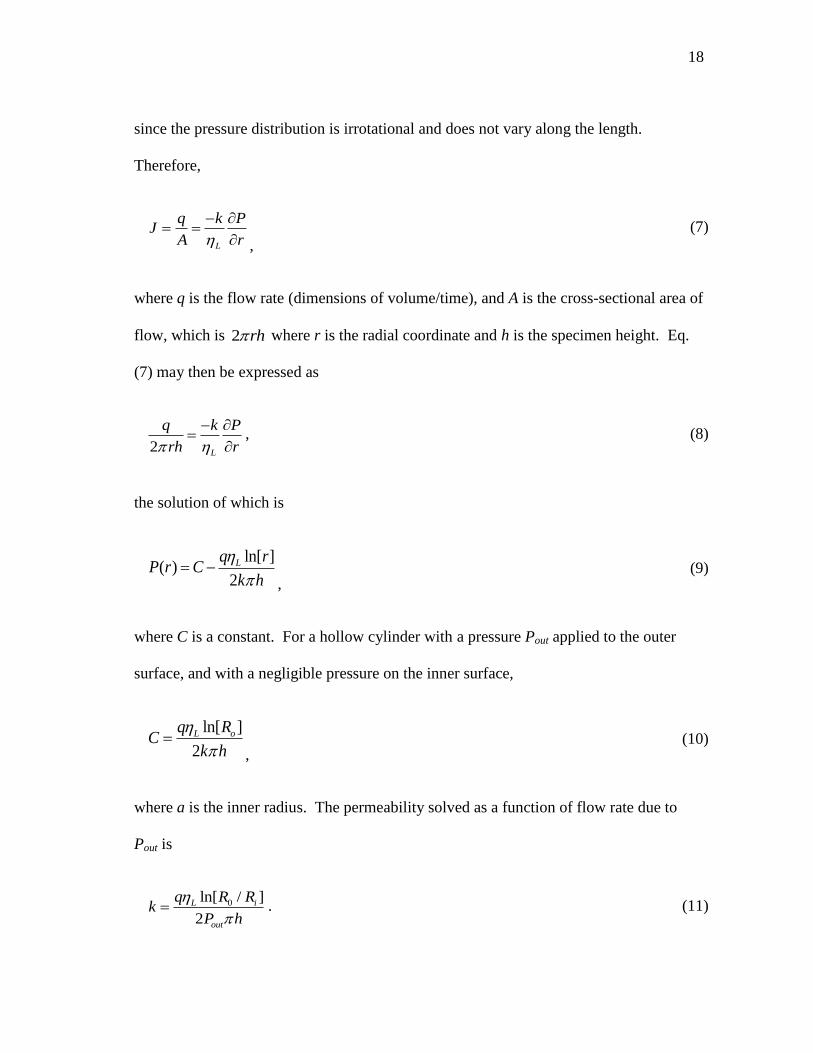
18

since the pressure distribution is irrotational and does not vary along the length.

Therefore,

L

q k PJ

A r

,

(7)

where q is the flow rate (dimensions of volume/time), and A is the cross-sectional area of

flow, which is 2 rh where r is the radial coordinate and h is the specimen height. Eq.

(7) may then be expressed as

2 L

q k P

rh r

, (8)

the solution of which is

ln[ ]

( )2

Lq rP r C

k h

, (9)

where C is a constant. For a hollow cylinder with a pressure Pout applied to the outer

surface, and with a negligible pressure on the inner surface,

ln[ ]

2

L oq RC

k h

, (10)

where a is the inner radius. The permeability solved as a function of flow rate due to

Pout is

0ln[ / ]

2

L i

out

q R Rk

P h

. (11)

19

4.2 HOLLOW DYNAMIC PRESSURIZATION

The general solution for the axial strain in a hollow poroelastic cylinder has been derived

by Kanj and Abouslemein [19, 20] and [21]. While this solution may be used to solve

the problem in the Laplace transform domain, it requires numerical inversion into the

time domain. In order to devise a simple approximate solution in the time domain, it is

useful to approach the problem in the same manner that Scherer [15] solved for the axial

strain in a solid poroelastic cylinder exposed to hydrostatic pressure. Viscoelastic

relaxation of the materials was not considered since Scherer [15] demonstrated that such

relaxation had a minimal effect on the outcome of the test.

The poroelastic constitutive equation for the axial plane strain ( z ) is

1

( ) ( , ) ( , ) ( , ) ( , )z z p r f

p

t r t r t r t r tE

,

(12)

where z , r , and are the axial, radial, and tangential stresses, pE is the Young‟s

modulus of the porous body, p is the Poisson‟s ratio of the porous body, and r and t are

the radial coordinate and time, respectively. The free strain is given by

( , )

( , )3

f

p

bP r tr t

K

,

(13)

where P is the pore pressure, pK is the bulk modulus of the porous body, and

20

1p

s

Kb

K (14)

is the Biot coefficient. sK is the bulk modulus of the solid material skeleton. Assuming

the pore fluid transport obeys Darcy‟s Law, the continuity equation may be expressed as

2( , )

( , ) ( , )L

P r t kb r t P r t

M

,

(15)

where k is the intrinsic permeability of the porous body (in dimensions of length

squared), L is the pore fluid viscosity, is the volumetric strain, the overhead dots

represent a partial time derivative, and

1/L s

bM

K K

(16)

is the Biot modulus. LK is the bulk modulus of the pore fluid and is the volumetric

pore fraction of the porous body.

In this problem, we are considering a porous hollow cylinder that is pressurized

hydrostatically. However, no fluid flow is allowed through the axial faces such that only

radial flow is considered. Therefore, eq. (15) becomes

2

( , ) 1 ( , )( , )

( )L o i

P u t k P u tb u t u

M R R u u u

(17)

21

where /( )o iu r R R is a dimensionless radial coordinate with r the radial coordinate,

Ro the outer radius of the cylinder, and Ri the inner radius of the cylinder. As with a

solid cylinder [15, 16], the volumetric strain of a hollow cylinder exposed to an applied

hydrostatic pressure PA is

( , ) 3 3 1 ( ) Af f

p

Pu t t

K (18)

where ( )f t is the volumetric average of the free strain such that

/( )

2 2

/( )

22( ) ( , ) ( , )

o o o i

i i o i

R R R R

o i

f f f o i

o i o iR R R R

R Rt r t rdr uR uR t udu

R R R R

. (19)

The constant is defined according to [15]

1

3 1

p

p

. (20)

By combining eqs. (13), (17), and (19) a partial differential equation for the pore

pressure is obtained in the same form as for a solid cylinder,

1 ( )( , ) ( ) 1 ( , )

1 1 1 1

Ab PP u P P u

ub b u u u

,

(21)

where

2

p

Mb

K Mb

. (22)

22

The dimensionless time is / vt where v is a relaxation time expressed as

2 2

0( ) 1L iv

p

R R b

k K M

,

(23)

which controls the rate of pore pressure equilibration. In comparison to the relaxation

time for the solid cylinder denoted in [15], the only difference in the expression for the

relaxation time of the hollow cylinder is that the radius of the solid cylinder, R, is

replaced by the term 0( )iR R .

The goal of the following discussion is to illustrate a method for deriving an

approximate analytical expression for v as a function of ( )z t in the time domain. The

solution of eq. (21) is readily obtained in the Laplace transform domain. The result is

the transformed pressure as a function of u and s (the reduced time transform variable).

Consider a step pressurization as a function of time, i.e.

( ) ( ) AP t H t P , (24)

where ( )H t is the Heaviside function and PA is the magnitude of the applied pressure.

In this case, the axial strain immediately after the pressurization is

0( ) (1 )3

Az

p

Pt b

K

,

(25)

which is the same as for a solid cylinder. The final strain after pressurization is

23

( )3

Az

s

Pt

K

, (26)

which is also the same as for a solid cylinder. The time-dependent axial strain may

therefore be expressed as

0( ) ( ) ( ) ( ) ( )z z z z , (27)

where ( ) is the compliance function. The Laplace transform of eq. (27) is simply

( ) ( 0) ( ) ( 0) ( )z s s s s s s s s (28)

where the overbars denote the Laplace transformed quantities, s is the transform

variable, and the initial and final value theorems of Laplace transforms are used.

The stresses in the hollow cylinder, ( , )r r t , ( , )r t , and ( , )z r t , can be determined

using the thermoelastic solution of a long, hollow cylinder [22] since thermal strains

caused by variations in temperature are analogous to the free strains (eq. (13)) caused by

changes in pore pressure. By combining the transformed stresses with the transform of

eq. (12) and ( , , / )o iP u s R R found by solving eq. (21) in the Laplace Transform domain,

( )z s was be determined as a function of P. Then, by substituting ( )z s into eq. (28),

( )s was determined. The answer was inverted numerically into the reduced time

domain with the Stehfest Algorithm [23, 25] to obtain ( ) . The relaxation functions

for a hollow cylinder and for a solid cylinder [15] are plotted in Figure 4.

24

Figure 4. Comparison of relaxation functions for solid and hollow cylinders. Note that the early

behavior (θ < 0.01) is comparable for both functions. In this case Ro/Ri is equal to 3.937 which

corresponds to a 10.16 cm (4 inch) diameter cylinder with a 2.54 cm (1 inch) diameter hole.

The important feature to recognize in Figure 4 is that at short times ( 0.01 ), the solid

and hollow cylinder functions are virtually identical. The implication is that the short-

time response of the hollow cylinder is able to be represented by the same function as

the solid cylinder, shown by Scherer [15] to be

4

( ) 1 1 1 b

.

(29)

As a result, the relaxation function over the full time span can be approximated by a

function of the form

0

0.2

0.4

0.6

0.8

1

0.0001 0.001 0.01 0.1 1

HollowSolid

25

4

( ) exp 1 11

m

nb

(30)

where m and n are fit parameters. For the hollow cylinder these fit parameters m and n

are dependent on the geometry of the specimen being tested, particularly the ratio of the

outer and inner radii (Ro/Ri). The equations for determining m and n are

0.19623

5.6152 o

i

Rm

R

(31)

and

1.8506

0.40086 0.0056243 o

i

Rn Ln

R

,

(32)

where the numerical coefficients are determined by curve fitting the m and n results of

several different radius ratios as shown in Figure 5 and Figure 6.

For the solid cylinder, equation (28) can also be used since the initial and final strains are

identical to those of the hollow cylinder. Equation (30) is also identical except that for

the solid cylinder the value of m=2.2 and the value of n=0.55 according to [15, 25].

Equation (23) changes to account for the lack of a hole in the center of the specimen to

become

2 2 1L

v

p

R b

k K M

, (33)

26

where R is simply the radius of the cylinder.

Figure 5: The fit parameter m is determined by curve fitting several different radius ratios.

2

2.5

3

3.5

4

4.5

5

5.5

6

1 10

m

Ro/R

i

27

Figure 6: The fit parameter n is determined by fitting the results of various radius ratios.

Figure 7 shows the numerically inverted data for ( ) fit by eq. (30). Using fit

parameters of 4.4924m and 0.4235n which correspond to a radius ratio of 4,

yielded an R2 value of 0.99983.

0.35

0.4

0.45

0.5

1 10

n

Ro/R

i

28

Figure 7. Approximation of the relaxation function Ω(θ) using eq. (30). The discrete points are

numerically inverted data for Ω(θ) while the solid line is the approximate function. The function is

evaluated using properties typical of concrete: β = 1/2, b = 2/3, λ = 1/4.

In order to obtain the permeability value of a given specimen, the strain versus time data

must be obtained through testing, and then fit using eq. (27). Eq. (30) must first be

substituted into (27), and the appropriate m and n values obtained from (31) and (32)

must be used to determine the value of τv from (27). Next, the values of ηL, Ro, and Ri

can be entered directly into (23). β can be calculated according to (20) using 0.2 as an

approximate value for νp. Kp and b can be determined from the strain time data and (25).

Finally, M can be calculated using (16) by assigning a value to KL (typically a textbook

value – e.g. 2.2 LK GPa for water) and by calculating Ks from the strain versus time

0

0.2

0.4

0.6

0.8

1

0.0001 0.001 0.01 0.1 1

29

data according to (26). The intrinsic permeability k may be determined directly by

substituting values of , v , Kp, M, b, ηL, Ro, and Ri into (23).

30

5 EXPERIMENTAL TECHNIQUES

5.1 SPECIMEN MATERIALS AND PREPARATION

In this study, Vycor glass and cement paste samples were tested for permeability. The

Vycor glass was type 7930 and was acquired in hollow tubes and solid rods. The tubes

and rods were 21 cm (8.25 in) long. The rods tested had a 6.35 mm (0.25 in) diameter

and the tubes had an inner diameter of 1.9 cm (0.75 in) and an outer diameter of 2.1 cm

(0.827 in). The rods and tubes were vacuum saturated in glycerol, a solution of glycerol

and water, or pure distilled water prior to testing depending on the type of testing to be

performed. The hollow cement paste samples were cast in 6.72 x 15.24 cm (3 x 6 in)

cylinder molds while the solid specimens were cast in 3.7 cm (1.45 in) tubes. The

hollow specimens additionally had a 3.7 cm (1.45 in) diameter hole cast down the center

through the length of the specimen. The cement used was a common Type I/II and was

mixed at w/c of 0.5 and 0.6.

The cement paste was mixed according to ASTM C305-99. To achieve the hollow

cylinder geometry, a thin walled polyethylene tube was glued into the center of the

cylinder mold and a hole was cut in the center of the lid to accommodate this tube. Both

the lid itself and the hole in the lid were sealed with silicone to prevent any moisture

from leaving the cylinder during initial curing. The specimens were de-molded at

approximately 12 hours and were immediately placed in a saturated lime water solution

31

to prevent any leaching of the internal calcium hydroxide. Additionally, the specimens

in the lime water were placed under vacuum to promote saturation.

The concrete cylinders were prepared using the mix design shown in Table 1. This mix

represents a typical bulk concreting mix that might be encountered in construction of a

driveway or sidewalk. The maximum nominal size of the coarse aggregate was 9.5 mm

(3/8 in). This relatively small coarse aggregate was chosen to ensure that a single

aggregate particle did not transverse the entire flow distance of the sample. Generally,

aggregates should be less than or equal to 1/3 of the flow distance within the cylinder

[18]. For a 7.62 cm (3 in) diameter specimen with a 1.27 cm (1/2 in) hole down the

center, 9.5 mm (3/8 in) aggregate is the largest that can be used and still satisfy this rule

of thumb.

Table 1: The concrete mix design used in the testing is representative of a typical driveway or

sidewalk mix.

Cement Type I/II 334 kg/m3564 lbs/yd3

Water 200 kg/m3 338 lbs/yd3

Coarse Aggregate (9.5mm max) 1232 kg/m3 2079 lbs/yd3

Fine Aggregate 610 kg/m31030 lbs/yd3

Concrete Mix Design

The concrete specimens were also cast with a 1.27 cm (1/2 in) diameter polythene tube

down the center of the cylinder in a standard 7.62 cm by 15.24 cm (3 in by 6 in) cylinder

32

mold. Lids were used during the initial curing and the samples were de-molded and

placed in lime water after approximately 12 hours.

The specimens were trimmed on a diamond blade wet saw to ensure that their ends were

uniform and parallel to one another. Steel plates were glued onto the ends of the hollow

cement paste specimens with a two-part marine epoxy to prevent any fluid from moving

through the axial faces of the specimen and to facilitate mounting inside the testing

apparatus. The Vycor glass tubes would have been similarly sealed, but the thin wall

thickness required caps which attached both to the ends as well as a small portion of the

side of the tube. These caps were also secured with the marine epoxy. The sealing of

the specimens is shown schematically in Figure 8. The solid rods were not sealed, but

due to their extremely slender nature very little fluid would flow through the ends

compared to the amount through the sides. As discussed in [15] and [25] the relaxation

time is affected by flow through the ends of a cylinder, though this effect is related to the

square of the length to width ratio. Since these solid specimens are extremely slender

(height to width ratio greater than 32 for the Vycor and 8 for the cement paste) this effect

will be extremely small and is neglected in this analysis.

33

Figure 8: The hollow Vycor and cement paste specimens are sealed at each end with special caps,

secured by a two part marine epoxy.

5.2 POROSITY DETERMINATION

One of the parameters necessary for determining k for both the SDP and HDP tests is the

specimen porosity. Vichit-Vadakan and Scherer [26] show that porosity of cementitious

materials determined by oven drying agrees with porosity measured by 2-propanol

exchange and is much quicker. In this study, the oven drying technique was used for

determining porosity. For the cement paste samples, this method involved obtaining a

small, representative disc of the material and saturating it under vacuum. The saturated

surface dry weight and the dimensions of the sample were obtained using a digital

balance capable of 0.001 gram accuracy and a digital caliper with 0.001 cm accuracy.

The sample was then placed in the oven at 110 degrees Celsius. After drying overnight,

the dry weight was obtained and the porosity was determined according to

Marine EpoxyHollow Cement

Paste

Steel Plate

Steel Plate

VycorGlass Tube

End Cap

End Cap

34

SSD OD

SSD Water

M M

V

,

(34)

where MSSD is the mass in the saturated surface dry state, MOD is the mass in the oven dry

state, VSSD is the measured volume in the saturated surface dry state, and ρWater is the

density of water.

For the Vycor glass, the dimensions of a solid rod were accurately measured using the

same digital caliper to determine its volume. The rod was then vacuum saturated and

weighed in the saturated surface dry condition. Finally, the rod was oven dried at 110

degrees Celsius and weighed again. The porosity of the Vycor was also calculated using

equation (34).

The initial porosity of the cement paste was determined from the mix design, and then at

subsequent ages with the oven drying test to establish a best fit curve for each material.

This curve was used to accurately estimate the porosity of a given specimen at a

particular age. The porosity of the Vycor glass was not time dependent and was not

tested at different ages. The cement paste porosity versus age plot is shown in Figure 9

with an exponential fit. The porosity of the Vycor glass is also shown in Figure 9 for

comparison purposes.

35

Figure 9: The porosity of the cement paste specimens as a function of age.

5.3 FLUID VISCOSITY DETERMINATION

One of the primary advantages of the dynamic pressurization technique is the increased

speed of each test. This advantage actually became a hindrance when the Vycor glass

was tested in water. The HDP test with the Vycor tube in water ran completely in

approximately 0.1 seconds (determined by calculation), so data collection was

impossible. As shown in equation (23) the relaxation time is directly related to the fluid

viscosity. By changing the viscosity of the testing fluid, the relaxation time of the test

could be adjusted to a more reasonable length of time. Glycerol was chosen as a

complimentary fluid to water for several reasons. First, glycerol is roughly 1,000 times

0.3

0.35

0.4

0.45

0.5

0.55

0.6

0.65

0.7

0 80 160 240 320 400 480 560 640

w/c = 0.5w/c = 0.6Vycor

Poro

sity

Age (Hours)

36

more viscous than water; this slowed the HDP test more than enough for reasonable data

collection to proceed. Additionally, the glycerol molecules are similar in size to water

molecules. This similarity is important because of the small average pore size in the

Vycor. Finally, glycerol and water are readily soluble in one another, which facilitates

custom viscosity blends.

In order to obtain the necessary inputs for the permeability calculations, a few values,

which are not obtained from either the SDP or HDP tests, must be determined. First, the

dynamic viscosity of the particular pore fluid used must be determined. The viscosity of

water is very well known [27], and it does not change very much with changes in

temperature. However, glycerol varies substantially with a small change in temperature

so the viscosity at laboratory temperature (~23 C) was determined using a Brookfield

rotational viscometer. The results of the viscosity testing are shown in Table 2.

Table 2: Since the Vycor tubes have a thin wall thickness, fluids with higher viscosities than water

were used to slow the Hollow Dynamic Pressurization test.

Fluid Viscosity (Pa-s)

Distilled Water 0.00102

65wt% Glycerol 0.0128

90wt% Glycerol 0.1823

Glycerol 1.067

5.4 FLUID BULK MODULUS DETERMINATION

In addition to the viscosity, the bulk modulus, KL, changes with each fluid blend.

Though not as influential in the final permeability determination as the viscosity, KL

37

must be accurately estimated in order to obtain sensible permeability results with the

dynamic pressurization techniques. In the case of pure water and pure glycerol this

determination was a simple matter of using a reference value obtained from a source

such as [27]. For the water/glycerol blends, the rule of mixtures,

1 1 2 2( ) ( )L Blend L LK f K f K , (35)

was employed to estimate the bulk modulus of the blend where KL-Blend is the bulk

modulus of the fluid blend, f1 is the volume fraction of liquid 1, KL-1 is the bulk modulus

of liquid 1, KL-2 is the bulk modulus of liquid 2 and f2 is the volume fraction of liquid 2.

The bulk moduli of the various liquids used in both the HDP and the SDP test are shown

in Table 3.

Table 3: The bulk modulus values for the testing fluid are used in calculating the permeability for

each specimen with the dynamic pressurization methods.

Fluid K L (Pa)

Distilled Water 2.2x109

65wt% Glycerol 3.57x109

90wt% Glycerol 4.23x109

Glycerol 4.52x109

5.5 TESTING PROGRAM

The general scheme in this experimental sequence was to first establish the HDP test as

accurate and repeatable by testing the Vycor glass. The permeability values obtained

from the HDP test were compared to those obtained with the SDP and RFT tests. This

38

allowed the comparison of the new HDP test to another poromechanical test and to a

direct flow through test. Once the validation had been established, cement paste

specimens were tested using the same HDP versus SDP and HDP versus RFT

comparison scheme. Finally a single concrete specimen was tested, with the HDP test, to

determine the applicability of the HDP technique to actual concrete.

39

6 RESULTS AND DISCUSSION

6.1 VYCOR

To validate the HDP method, Vycor glass specimens were tested using the HDP, SDP

and RFT techniques. The results from the RFT and the SDP were each compared to the

results obtained from the HDP test to determine the equivalency of the results.

The final input parameter required for calculating permeability for both the SDP and

HDP techniques is a strain-time history, which can be fit to determine the relaxation

time, τv, and ultimately the permeability of the material. Figure 10 shows a typical

strain-time history for the HDP test, shown on both the time and log-time axes. These

results are for a hollow Vycor tube tested in pure glycerol. The plots show that

equilibrium is reached in approximately nine hours, which is roughly equivalent to the

fit parameter τv.

40

Figure 10: Typical hollow dynamic pressurization strain data shown on time and log-time axes. The

log-time axis more clearly shows when the specimen has fully relaxed.

6.1.1 Hollow Dynamic Pressurization Versus Radial Flow Through

In order to facilitate the most direct comparison possible between the RFT and the HDP,

two intermediate fluid blends were created with viscosities that fell in between that of

water and pure glycerol. The viscosities of the blends were intentionally optimized to

allow the HDP test to run quickly. Water was used only for the flow through and the

100% glycerol was only used for the HDP. Multiple repetitions of each test were

conducted to establish a valid statistical comparison with these combinations. The

combined results are shown in Table 4 with the associated means and standard

deviations.

-180

-160

-140

-120

-100

-80

-60

0 5 10 15 20 25

Str

ain

(1

0-6

)

Time (h)

-160

-150

-140

-130

-120

-110

-100

-90

0.0001 0.001 0.01 0.1 1 10 100

Str

ain

(1

0-6

)Time (h)

41

Table 4: The tabulated results of the Vycor permeability testing show good agreement between the

various test permutations of fluid and test method.

Trial Glycerol 65wt% Glycerol 90wt% Glycerol Water 65wt% Glycerol

1 0.021 0.018 0.023 0.016 0.012

2 0.024 0.019 0.030 0.028 0.014

3 0.020 0.015 0.026 0.025 0.019

4 0.032 0.018 0.021 0.013 0.014

5 0.014 0.015 0.021 0.017 0.016

6 0.028 0.017 0.021 0.018 0.020

7 0.034 0.019 0.023 0.022 0.015

8 0.019 0.023 0.020 0.023 0.016

9 0.018 0.017 0.024

10 0.019 0.015 0.021

11 0.016 0.023

12 0.036

13 0.024

Mean 0.02409 0.01808 0.02113 0.02239 0.01559

12.77%28.46% 20.79%

Combined

COV29.58%24.46%

Coeficient

of

Variation

17.11%26.01%

Hollow Flow Through ResultsHollow Dynamic Pressurization Results

Permeability (nm2) Permeability (nm

2)

Standard

Deviation0.00685 0.00231 0.00582 0.002670.00439

The maximum difference in the measured permeability values reported in Table 4

(between the flow through test using 65% glycerol and the HDP test using glycerol) is a

mere 35%. When the exact same fluid was used in the flow through and HDP tests (both

used 65% glycerol), the percent difference in mean permeabilities between the

techniques was only 23%. The HDP test shows excellent repeatability with these means

falling very close to one another.

42

With the HDP and the RFT technique, the greatest coefficient of variation was 28%, and

the greatest combined coefficient of variation was 30% which are both near the lower

end of the range of typical variability of permeability measurements [8, 28, 29].

Additionally, the results shown in Table 4 agree reasonably well with the Vycor

permeability results obtained by Vichit-Vidakan and Scherer [30] both in mean and in

standard deviation.

When evaluating the agreement in means of two data sets the Student‟s T-Test is

frequently employed. For this test a characteristic „t‟ statistic is calculated according to

1 2

2 2

1 2

ts s

m n

(36)

where µ1 is the mean of the first data set, µ2 is the mean of the second data set, Δ is the

null value, s1 is the standard deviation of the first data set, s2 is the standard deviation of

the second set, m is the number of data points in the first data set, and n is the number of

data points in the second set [31]. This „t‟ value is then compared to a reference value

based on the confidence level and the number of data points in the combined data set.

Typically, results are tested at the 95% confidence level, which means that the

determination is predicted to be correct 95% of the time. By using the reference value

corresponding to the 95% confidence level and the appropriate number of data points,

the null value Δ can be determined. Once the Δ value is obtained the percent difference

can be determined according to,

43

1 2

% 100( ) / 2

percent difference

(37)

With the data presented in Table 4 it can be shown that the percent difference in the

permeability values from the HDP test and the RFT test will be 5.4% or less 95% of the

time; this difference is much smaller than the typical coefficient of variation reported in

literature [8, 28, 29] for permeability of cementitious materials obtained with a single

test method.

From a practical perspective, the percent difference between the Vycor glass

permeability measured using the flow through technique and the HDP technique is

statistically insignificant. Therefore, the HDP test has been successfully validated and

has been shown to yield the same permeability as a flow-through test for Vycor glass.

6.1.2 Hollow Dynamic Pressurization Versus Solid Dynamic Pressurization

The results from the testing of hollow and solid Vycor specimens for permeability show

good correlation between the HDP and the SDP techniques. The difference between the

average permeability determined from the HDP and the SDP is 13%. The permeability

values for the Vycor specimens are presented in Table 5.

44

Table 5: The measured Vycor permeability and associated statistical quantities measured with

various fluids.

Trial Glycerol 65wt% 90wt% Glycerol 65wt%

1 0.021 0.018 0.023 0.038 0.008

2 0.024 0.019 0.030 0.011 0.013

3 0.020 0.015 0.026 0.013 0.012

4 0.032 0.018 0.021 0.024 0.009

5 0.014 0.015 0.021 0.024 0.008

6 0.028 0.017 0.021 0.031 0.009

7 0.034 0.019 0.023 0.019 0.014

8 0.019 0.023 0.020 0.035 0.016

9 0.018 0.017 0.018

10 0.019 0.015 0.018

11 0.016

Average 0.024086 0.018081 0.021126 0.0244 0.0122776

Standard

Deviation 0.006854 0.00231 0.004392 0.00982 0.0040541

Coeficient of

Variation 28.46% 12.77% 20.79% 40.26% 33.02%

Permeability (nm2) Permeability (nm

2)

Solid DP Results

Combinded

Coeficient of

Variation 52.75%24.46%

Hollow DP Results

Typical concrete permeability tests show high variability between repetitions. Reported

coefficients of variation between 20% and 130% [8, 28, 29] are typical of this type of

testing. With the hollow and the SDP techniques, the greatest coefficient of variation

was 40%, and the greatest combined coefficient of variation was 53%, which are both

toward the lower end of this range. Additionally, the results shown in Table 5 agree

reasonably well with the Vycor permeability results obtained by Vichit-Vidakan and

Scherer [30] both in mean and in standard deviation.

45

With the data presented in Table 5 it can be shown that the percent difference in the

permeability values from the HDP test and the SDP test will be 17% or less 95% of the

time; this difference is much smaller than the typical coefficient of variation reported in

literature [29] for permeability of cementitious materials obtained with a single test

method.

From a practical perspective, the percent difference between the Vycor glass

permeability measured using the SDP technique and the HDP technique is statistically

insignificant. Therefore, the HDP test has been successfully validated and has been

shown to yield the same permeability as the SDP test for Vycor glass.

6.2 CEMENTITIOUS MATERIALS

In order to obtain a statistically significant amount of data in a reasonable length of time

with the RFT test, specimens with a w/c of 0.6 were chosen for their relatively high

permeability. Choosing specimens with high permeability helps the RFT test to run

more quickly while reducing the risk of leaking since the fluid will be more likely to

flow through the specimen than through any sealed connection. For the SDP to HDP

comparison, a w/c of 0.5 was chosen because the specimens are simpler to cast and there

is no real need for increased speed with the dynamic pressurization techniques.

46

6.2.1 Hollow Dynamic Pressurization Versus Radial Flow Through

The difference between a low permeability material and a high permeability material is

worth noting. The difference between a 0.5 w/c paste and a 0.6 w/c paste is reported as a

full order of magnitude (i.e. 0.001 nm2 as compared to 0.01 nm

2) by Grasley et al. [26];

this difference in measured permeability is a change of 900%. Based on the results

shown in Table 6, the difference between the mean values of the two methods is 32%.

This level of sensitivity is clearly sufficient to discern two different construction

materials.

Using equations (36), (37), and the data presented in Table 6, the percent difference

between the results obtained with the HDP test and the RFT test will be 38% or less 95%

of the time. This value is higher than that obtained with the Vycor glass principally

because of the material variability in the cement paste.

47

Table 6: The permeability results from the 0.6 w/c paste show good correlation between the HDP

and the radial flow through techniques.

Hollow Dynamic Pressurization Radial Flow Through

Trial Permeability (nm2) Permeability (nm

2)

1 0.414 0.339

2 0.370 0.289

3 0.364 0.260

4 0.496 0.279

5 0.400 0.277

6 0.426 0.316

7 0.502 0.300

8 0.375 0.298

9 0.500 0.253

Mean 0.42751 0.29005

Coeficient

of Variation

13.47% 9.25%

Standard

Deviation0.05760 0.02682

Additionally, it should be noted that the 32% difference is between two totally different

test methods. The ranges reported by Banthia and Mindess in [29], and for most other

studies, were representative of a single test method. The small differences between the

HDP and the RFT results could be due to material differences between the two samples

used for the two tests or an inherent, systematic difference in the two test methods.

Material differences between the two samples were kept to a minimum since the samples

were cast from the same mix, and were cured identically. Additionally the inherent

nature of cement paste is very homogeneous and lends itself to good consistency. With

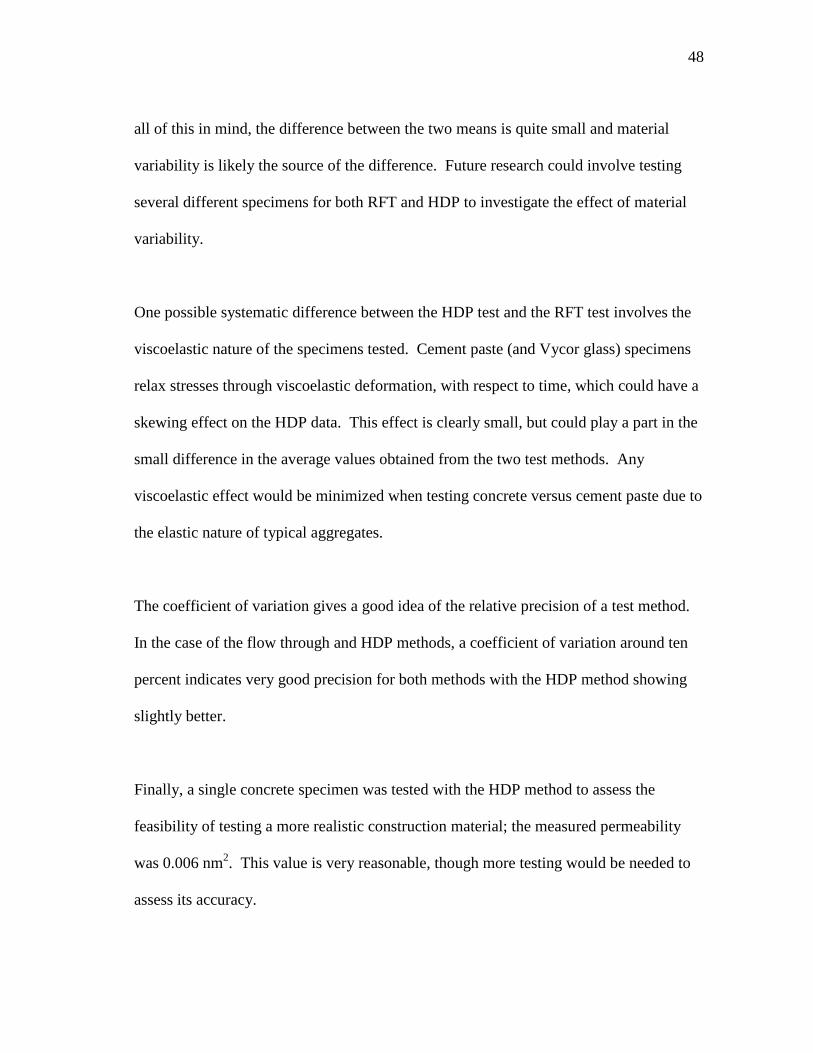
48

all of this in mind, the difference between the two means is quite small and material

variability is likely the source of the difference. Future research could involve testing

several different specimens for both RFT and HDP to investigate the effect of material

variability.

One possible systematic difference between the HDP test and the RFT test involves the

viscoelastic nature of the specimens tested. Cement paste (and Vycor glass) specimens

relax stresses through viscoelastic deformation, with respect to time, which could have a

skewing effect on the HDP data. This effect is clearly small, but could play a part in the

small difference in the average values obtained from the two test methods. Any

viscoelastic effect would be minimized when testing concrete versus cement paste due to

the elastic nature of typical aggregates.

The coefficient of variation gives a good idea of the relative precision of a test method.

In the case of the flow through and HDP methods, a coefficient of variation around ten

percent indicates very good precision for both methods with the HDP method showing

slightly better.

Finally, a single concrete specimen was tested with the HDP method to assess the

feasibility of testing a more realistic construction material; the measured permeability

was 0.006 nm2. This value is very reasonable, though more testing would be needed to

assess its accuracy.

49

6.2.2 Hollow Dynamic Pressurization Versus Solid Dynamic Pressurization

In order to generate the most direct comparison possible, the HDP and the SDP methods

were performed on hollow and solid cement paste specimens beginning approximately

90 hours after the specimens were cast. Specifically, a hollow specimen was tested in

one pressure vessel and a solid specimen in a companion pressure vessel, with the test

beginning at effectively the same moment. At these early ages many test repetitions

could be obtained in a reasonably short period of time. By simultaneously testing these

samples, the effect of any age differences between specimens was avoided since the

solid sample was the same age as the hollow sample and vice versa. Since the hollow

and solid specimens were cast from the same mix, and were tested at an identical age,

the permeability results from the two tests can be readily compared at a given age to

evaluate the new HDP method.

For comparison purposes, permeability data from the literature was also included to

compliment the data collected in this study. Cement paste with a w/c of 0.6 was tested

by Vichat-Vidakan and Scherer [26] using the beam bending technique and these results

are plotted along with those gathered in this study using the HDP and SDP techniques in

Figure 11.

50

Figure 11: The results of the hollow dynamic pressurization test and the solid dynamic

pressurization tests shown as a function of age. For comparison purposes the results from some

other studies are included.

The results presented in Figure 11 show good agreement between the SDP and HDP

methods over the range of time that the data was collected. The differences between the

two methods could be attributable to some curing differences stemming from the

geometry of the specimens. As mentioned previously, the results from the HDP and

SDP tests on the 0.5 w/c paste are clearly much different than the results of the beam

bending test on the 0.6 w/c paste. Also the variability of the HDP and SDP tests appears

to be similar based on the scatter in the data points when compared to the beam bending

data.

0.001

0.01

0.1

1

100 150 200 250 300 350

0.5 HDP

0.5 SDP

0.6 BB (Vichat-Vidakan & Scherer)

Pe

rme

ab

ility

(n

m2)

Age (hours)

51

7 SUMMARY

Since saturated permeability of a material provides insight into the interconnectivity of

the pore network of that material and since no widely accepted concrete permeability test

exists, the Hollow Dynamic Pressurization (HDP) test is presented as an accurate and

repeatable method for measuring the permeability of cementitious materials. The hollow

specimen geometry allows for the saturation of the pore network of the specimen by

applying a hydrostatic pressure to the outer radial surface of the unsaturated specimen

which forces fluid into the pore network and forces air bubbles out. Since saturation is a

rigorous requirement of the dynamic pressurization technique, the ability to saturate an

existing specimen represents a major advantage over the solid dynamic pressurization

(SDP) technique. The HDP test is more rapid than traditional flow through techniques

and shows excellent repeatability both with Vycor glass and with cement paste. To

evaluate this new method, the HDP test was compared to the SDP test and to the radial

flow through (RFT) technique.

By comparing the results obtained from the HDP, SDP, and RFT tests, the HDP test has

been validated since the values were essentially identical to those obtained with the other

test methods. The coefficient of variation obtained with the HDP test is much lower

than for other permeability tests reported in the literature [8, 28, 29]. The particular

permeability values obtained agreed reasonably well with values obtained in literature

for similar materials. With all of the above in mind, the new HDP test shows promise as

an acceptable permeability test for cementitious materials.

52

REFERENCES

[1] Vitaliano, D.F., Infrastructure costs of road salting. Resources, Conservation

and Recycling, 7 (1-3) (1992) 171-180.

[2] Mehta, K., High-performance concrete durability affected by many factors,

Concrete Construction, 37 (5) (1992) 367-370.

[3] Gillott, J.E., Review of expansive alkali-aggregate reactions in concrete,

Journal of Materials in Civil Engineering, 7 (4) (1995) 278-282.

[4] Haynes, H., R. O'Neill, and P.K. Mehta, Concrete deterioration from physical

attack by salts, Concrete International, 18 (1) (1996) 63-69.

[5] Neville, A., Chloride attack of reinforced concrete: An overview, Materials

and Structures/Materiaux et Constructions, 28 (176) (1995) 63-70.

[6] Mehta, P.K., Durability of concrete - the zigzag course of progress, Indian

Concrete Journal, 80 (8) (2006) 9-16.

[7] Neville, A., Suggestions of research areas likely to improve concrete,

Concrete International, 18 (5) (1996) 44-49.

[8] Ye, G., P. Lura, and K. Van Breugel, Modelling of water permeability in

cementitious materials, Materials and Structures/Materiaux et Constructions,

39 (293) (2006) 877-885.

[9] Hearn, N. and R.H. Mills, Simple permeameter for water or gas flow, Cement

and Concrete Research, 21 (2-3) (1991) 257-261.

[10] Hooton, R.D. Permeability and pore structure of cement pastes containing

flyash, slag, and silica fume (1986). Denver, CO, ASTM, Philadelphia, PA.

[11] Scherer, G.W., Poromechanics analysis of a flow-through permeameter with

entrapped air, Cement and Concrete Research, 38 (3) (2008) 368-378.

[12] Scherer, G.W., J.J. Valenza, II, and G. Simmons, New methods to measure

liquid permeability in porous materials. Cement and Concrete Research, 37

(3) (2007) 386-397.

[13] Scherer, G.W., Measuring permeability of rigid materials by a beam-bending

method: I, theory, Journal of the American Ceramic Society, 83 (9) (2000)

2231-2239.

53

[14] Scherer, G.W., Thermal expansion kinetics: Method to measure permeability

of cementitious materials. I. Theory, Journal of the American Ceramic

Society, 83 (11) (2000) 2753-2761.

[15] Scherer, G.W., Dynamic pressurization method for measuring permeability

and modulus: I. Theory, Materials and Structures/Materiaux et Constructions,

39 (294) (2006) 1041-1057.

[16] Gross, J. and G.W. Scherer, Dynamic pressurization: Novel method for

measuring fluid permeability, Journal of Non-Crystalline Solids, 325(1-3)

(2003) 34-47.

[17] Bhargava, A. and N. Banthia, Measurement of concrete permeability under

stress, Experimental Techniques, 30 (5) (2006) 28-31.

[18] El-Dieb, A.S. and R.D. Hooton, High pressure triaxial cell with improved

measurement sensitivity for saturated water permeability of high performance

concrete, Cement and Concrete Research, 24 (5) (1994) 854-862.

[19] Abousleiman, Y.N. and M.Y. Kanj, The generalized lame problem-part ii:

Applications in poromechanics, Journal of Applied Mechanics, Transactions

of the ASME, 71 (2) (2004) 180-189.

[20] Kanj, M.Y. and Y.N. Abousleiman, The generalized lame problem - part i:

Coupled poromechanical solutions. Journal of Applied Mechanics,

Transactions ASME, 71 (2) (2004) 168-179.

[21] Sawaguchi, H. and M. Kurashige, Constant strain-rate compression test of a

fluid-saturated poroelastic sample with positive or negative Poisson's ratio,

Acta Mechanica, 179 (3-4) (2005) 145-56.

[22] Sherief, H.H., A.E.M. Elmisiery, and M.A. Elhagary, Generalized

thermoelastic problem for an infinitely long hollow cylinder for short times,

Journal of Thermal Stresses, 27 (10) (2004) 885-902.

[23] Stehfest, H., Numerical inversion of Laplace transforms, Communications of

the ACM, 13 (1) (1970) 47-49.

[24] Wolfram Research, Numerical inversion performed using the package

NumericalInversion, © Mallet, A. 2000, University of Mauritius. in Wolfram

Research, Inc,: Champaign, IL.

54

[25] Grasley, Z.C., Scherer, G.W., Lange, D.A., and Valenza, J.J., Dynamic

pressurization method for measuring permeability and modulus: II.

Cementitious materials, Materials and Structures/Materiaux et Constructions,

40 (7) (2007) 711-721.

[26] Vichit-Vadakan, W., G.W. Scherer, and M. Grutzeek, Measuring permeability

of rigid materials by a beam-bending method: III, cement paste, Journal of the

American Ceramic Society, 85 (6) (2002) 1537-1544.

[27] Munson, B.R., Young, Donald F., and OIkiishi, Theodore H., Fundamentals

of fluid mechanics, 4th ed, John Wiley and Sons Inc, Hoboken, NJ. 2002

[28] Hooton, R.D., Permeability and pore structure of cement pastes containing fly

ash, slag, and silica fume, Denver, CO: ASTM, Philadelphia, PA, (1986)

[29] Banthia, N. and S. Mindess, Water permeability of cement paste, Cement and

Concrete Research, 19 (5) (1989) 727-736.

[30] Vichit-Vadakan, W. and G.W. Scherer, Measuring permeability of rigid

materials by a beam-bending method: II. Porous glass, Journal of the

American Ceramic Society, 83 (9) (2000) 2240-2245.

[31] Devore, J.L., Probability and statisitics. 6 ed, Brooks/Cole-Thompson

Learning, Belmont, CA, 2004

55

APPENDIX A. VYCOR PLOTS

VYCOR FLOW THROUGH PLOTS

65% Glycerol

Figure A- 1: Measured displacement versus time response of a Vycor tube sample when tested in 65

weight percent glycerol.

0

10

20

30

40

50

60

70

80

5000 1 1041.5 10

42 10

42.5 10

43 10

43.5 10

4

y = -12.974 + 0.0028922x R2= 0.99625

Dis

pla

cem

en

t (I

nch

esx1

0-3

)

Time (s)

56


weight percent glycerol.


weight percent glycerol. The stair-step nature of the data is due to minor sticking of the float within

the test apparatus.

0

10

20

30

40

50

60

5000 1 104

1.5 104

2 104

2.5 104

3 104

y = -0.48671 + 0.0025441x R2= 0.98134

Dis

pla

cem

en

t (I

nch

esx1

0-3

)

Time (s)

0

20

40

60

80

100

120

5000 1 1041.5 10

42 10

42.5 10

43 10

43.5 10

44 10

4

y = 4.1039 + 0.0026449x R2= 0.98962

Dis

pla

cem

en

t (I

nch

esx1

0-3

)

Time (s)

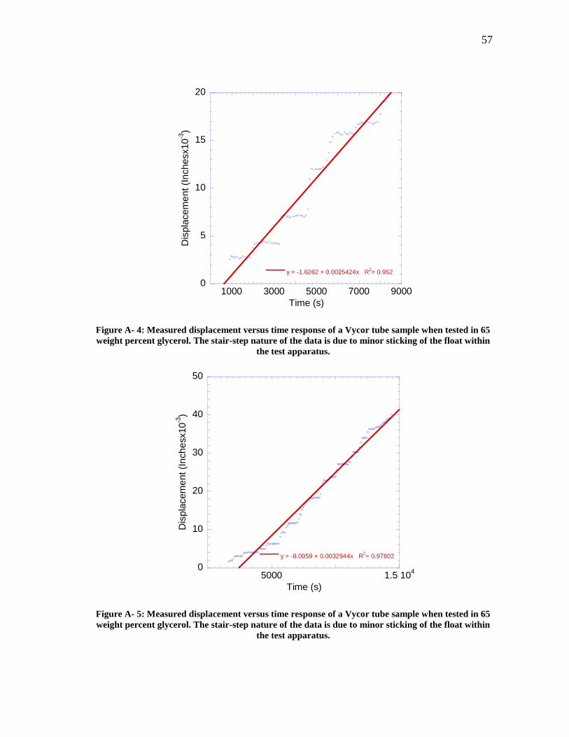
57



the test apparatus.



the test apparatus.

0

5

10

15

20

1000 3000 5000 7000 9000

y = -1.6262 + 0.0025424x R2= 0.952

Dis

pla

cem

en

t (I

nch

esx1

0-3

)

Time (s)

0

10

20

30

40

50

5000 1.5 104

y = -8.0059 + 0.0032944x R2= 0.97802

Dis

pla

cem

en

t (I

nch

esx1

0-3

)

Time (s)

58



the test apparatus.



the test apparatus.

0

10

20

30

40

50

60

70

80

5000 1.5 104

2.5 104

3.5 104

y = -12.819 + 0.0028809x R2= 0.99621

Dis

pla

cem

en

t (I

nch

esx1

0-3

)

Time (s)

0

10

20

30

40

50

2000 4000 6000 8000 1 1041.2 10

41.4 10

41.6 10

4

y = 6.4099 + 0.002676x R2= 0.94014

Dis

pla

cem

en

t (I

nch

esx1

0-3

)

Time (s)

59



the test apparatus.

10

15

20

25

30

35

40

45

1000 2000 3000 4000 5000 6000 7000 8000

y = 14.343 + 0.0036359x R2= 0.98673

Dis

pla

cem

en

t (I

nch

esx1

0-3

)

Time (s)

60

Water

Figure A- 9: Measured displacement versus time response of a Vycor tube sample when tested in

water with an applied hydrostatic pressure of 414 kpa (60 psi).



0

20

40

60

80

100

2000 4000 6000 8000 1 104

1.2 104

y = -23.064 + 0.010497x R2= 0.99007

Dis

pla

cem

en

t (I

nch

esx1

0-3

)

Time (s)

0

10

20

30

40

50

60

70

80

1000 2000 3000 4000 5000 6000 7000 8000

y = -13.76 + 0.010872x R2= 0.98078

Dis

pla

cem

en

t (I

nch

esx1

0-3

)

Time (s)

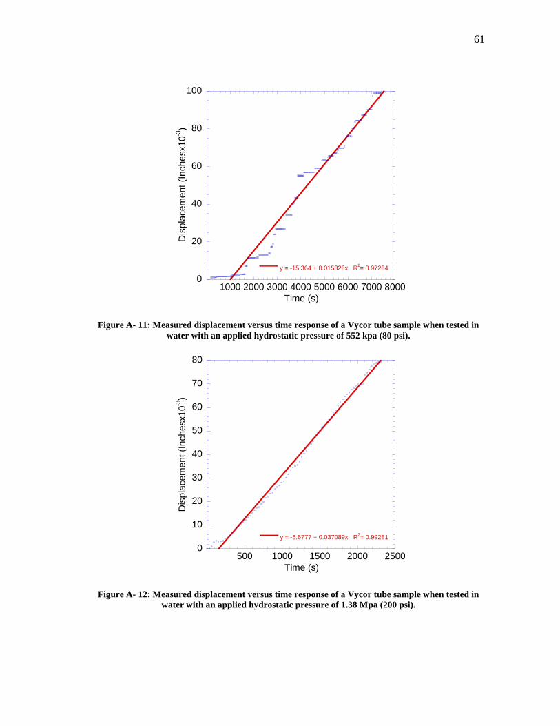
61




water with an applied hydrostatic pressure of 1.38 Mpa (200 psi).

0

20

40

60

80

100

1000 2000 3000 4000 5000 6000 7000 8000

y = -15.364 + 0.015326x R2= 0.97264

Dis

pla

cem

en

t (I

nch

esx1

0-3

)

Time (s)

0

10

20

30

40

50

60

70

80

500 1000 1500 2000 2500

y = -5.6777 + 0.037089x R2= 0.99281

Dis

pla

cem

en

t (I

nch

esx1

0-3

)

Time (s)

62





0

20

40

60

80

100

120

500 1000 1500 2000 2500 3000 3500

y = -21.081 + 0.035926x R2= 0.99391

Dis

pla

cem

en

t (I

nch

esx1

0-3

)

Time (s)

0

20

40

60

80

100

120

500 1000 1500 2000 2500 3000 3500

y = -0.41362 + 0.033968x R2= 0.99273

Dis

pla

cem

en

t (I

nch

esx1

0-3

)

Time (s)

63





0

20

40

60

80

100

120

500 1000 1500 2000 2500 3000

y = -11.721 + 0.0404x R2= 0.99016

Dis

pla

cem

en

t (I

nch

esx1

0-3

)

Time (s)

0

20

40

60

80

100

120

500 1000 1500 2000 2500 3000

y = -1.1193 + 0.03845x R2= 0.99559

Dis

pla

cem

en

t (I

nch

esx1

0-3

)

Time (s)

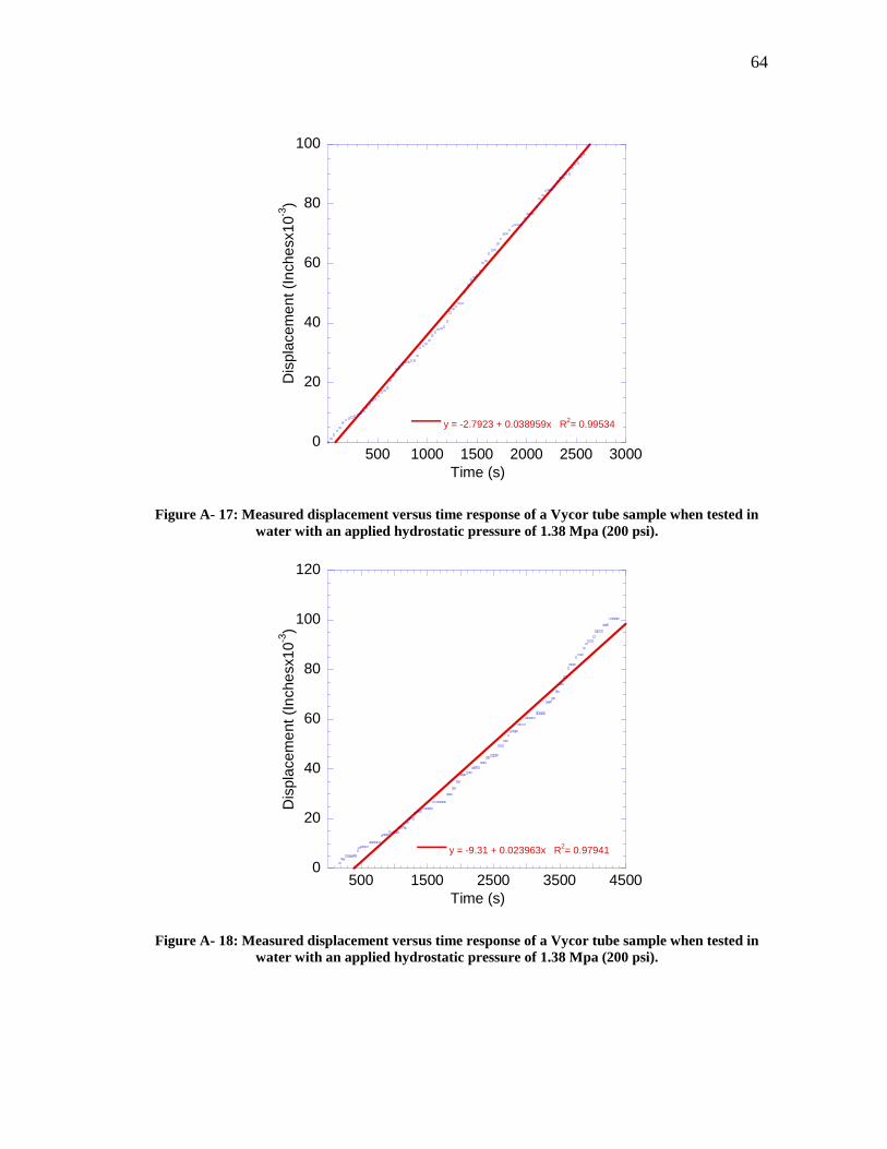
64





0

20

40

60

80

100

500 1000 1500 2000 2500 3000

y = -2.7923 + 0.038959x R2= 0.99534

Dis

pla

cem

en

t (I

nch

esx1

0-3

)

Time (s)

0

20

40

60

80

100

120

500 1500 2500 3500 4500

y = -9.31 + 0.023963x R2= 0.97941

Dis

pla

cem

en

t (I

nch

esx1

0-3

)

Time (s)

65





0

20

40

60

80

100

1000 2000 3000 4000 5000 6000

y = 1.1714 + 0.020584x R2= 0.99048

Dis

pla

cem

en

t (I

nch

esx1

0-3

)

Time (s)

0

20

40

60

80

100

500 10001500200025003000350040004500

y = -7.6487 + 0.02542x R2= 0.99214

Dis

pla

cem

en

t (I

nch

esx1

0-3

)

Time (s)

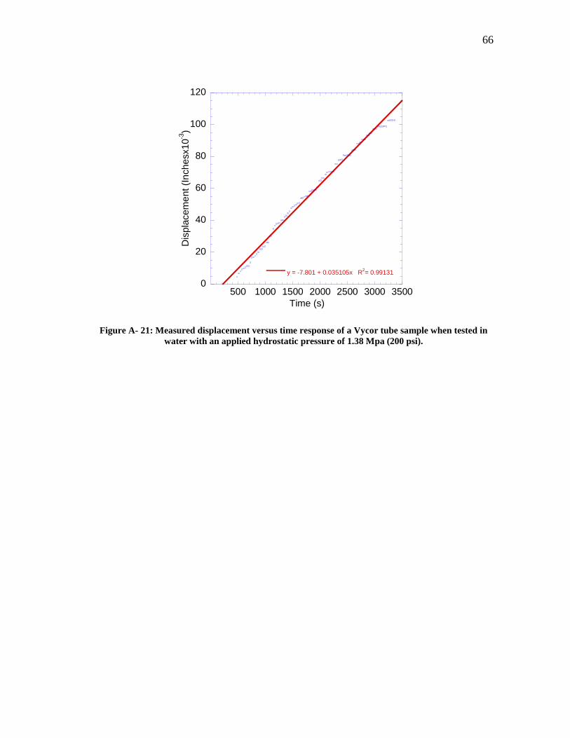
66



0

20

40

60

80

100

120

500 1000 1500 2000 2500 3000 3500

y = -7.801 + 0.035105x R2= 0.99131

Dis

pla

cem

en

t (I

nch

esx1

0-3

)

Time (s)

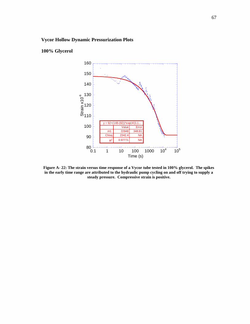
67

Vycor Hollow Dynamic Pressurization Plots

100% Glycerol

Figure A- 22: The strain versus time response of a Vycor tube tested in 100% glycerol. The spikes

in the early time range are attributed to the hydraulic pump cycling on and off trying to supply a

steady pressure. Compressive strain is positive.

80

90

100

110

120

130

140

150

160

0.1 1 10 100 1000 104

105

Str

ain

x1

0-6

Time (s)

y = 92+(148-(92))*exp(4/(3.1...

ErrorValue

348.9122948m1

NA2342.4Chisq

NA0.97771R2

68







90

100

110

120

130

140

150

160

170

0.1 1 10 100 1000 104

105

Str

ain

x1

0-6

Time (s)

y = 98+(154-(98))*exp(4/(3.1...

ErrorValue

340.1119815m1

NA3467.3Chisq

NA0.97696R2

80

90

100

110

120

130

140

150

160

0.1 1 10 100 1000 104

105

Str

ain

x1

0-6

Time (s)

y = 88+(155-(88))*exp(4/(3.1...

ErrorValue

380.829631m1

NA3243.5Chisq

NA0.98822R2

69







80

90

100

110

120

130

140

150

0.1 1 10 100 1000 104

Str

ain

x1

0-6

Time (s)

y = 88+(145-(88))*exp(4/(3.1...

ErrorValue

270.6610960m1

NA4518.2Chisq

NA0.94422R2

80

90

100

110

120

130

140

0.1 1 10 100 1000 104

105

Str

ain

x1

0-6

Time (s)

y = 84+(135-(84))*exp(4/(3.1...

ErrorValue

343.3226162m1

NA1412.6Chisq

NA0.98191R2

70

Figure A- 27: The strain versus time response of a Vycor tube tested in 100% glycerol. Compressive

strain is positive.




90

100

110

120

130

140

150

160

0.1 1 10 100 1000 104

Str

ain

x1

0-6

Time (s)

y = 90+(150-(90))*exp(4/(3.1...

ErrorValue

324.7412386m1

NA2015.1Chisq

NA0.9681R2

60

80

100

120

140

160

0.1 1 10 100 1000 104

105

Str

ain

x1

0-6

Time (s)

y = 60+(152-(60))*exp(4/(3.1...

ErrorValue

2740.41.0325e+05m1

NA14451Chisq

NA0.92163R2

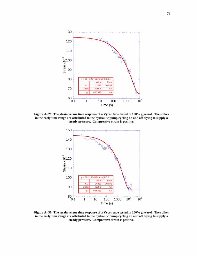
71







60

70

80

90

100

110

120

130

0.1 1 10 100 1000 104

Str

ain

x1

0-6

Time (s)

y = 65+(125-(65))*exp(4/(3.1...

ErrorValue

202.5313032m1

NA2158.6Chisq

NA0.97075R2

80

90

100

110

120

130

140

150

0.1 1 10 100 1000 104

105

Str

ain

x1

0-6

Time (s)

y = 88+(145-(88))*exp(4/(3.1...

ErrorValue

306.0116363m1

NA4185.6Chisq

NA0.96581R2

72

Figure A- 31: The strain versus time response of a Vycor tube tested in 100% glycerol. Compressive

strain is positive.

60

80

100

120

140

160

0.1 1 10 100 1000 104

105

Str

ain

x1

0-6

Time (s)

y = 75+(135-(75))*exp(4/(3.1...

ErrorValue

515.0423904m1

NA7144.9Chisq

NA0.96508R2

73

90% Glycerol

Figure A- 32: The strain versus time response of a Vycor tube tested in 90 weight percent glycerol.

Compressive strain is positive.



100

120

140

160

180

200

220

0.1 1 10 100 1000 104

Str

ain

x1

0-6

Time (s)

y = 108+(210-(108))*exp(4/(3...

ErrorValue

10.7691103.2m1

NA1672.2Chisq

NA0.99192R2

100

120

140

160

180

200

0.1 1 10 100 1000 104

Str

ain

x1

0-6

Time (s)

y = 118+(200-(118))*exp(4/(3...

ErrorValue

6.6786814.88m1

NA866.68Chisq

NA0.99511R2

74





120

140

160

180

200

220

0.1 1 10 100 1000

Str

ain

x10

-6

Time (s)

y = 135+(218-(135))*exp(4/(3...

ErrorValue

13.222787.53m1

NA3174.7Chisq

NA0.97962R2

120

140

160

180

200

220

0.1 1 10 100 1000 104

Str

ain

x1

0-6

Time (s)

y = 137+(220-(137))*exp(4/(3...

ErrorValue

22.9641163m1

NA4875.9Chisq

NA0.97245R2

75





130

140

150

160

170

180

190

200

210

0.1 1 10 100 1000 104

Str

ain

x1

0-6

Time (s)

y = 137+(220-(137))*exp(4/(3...

ErrorValue

19.1351073.8m1

NA3557.3Chisq

NA0.97579R2

120

140

160

180

200

220

0.1 1 10 100 1000 104

Str

ain

x1

0-6

Time (s)

y = 125+(212-(125))*exp(4/(3...

ErrorValue

19.5021338.2m1

NA3196.4Chisq

NA0.98128R2

76





120

140

160

180

200

220

0.1 1 10 100 1000 104

Str

ain

x1

0-6

Time (s)

y = 135+(215-(135))*exp(4/(3...

ErrorValue

48.3242092.2m1

NA8368.3Chisq

NA0.96735R2

120

140

160

180

200

220

0.1 1 10 100 1000 104

Str

ain

x1

0-6

Time (s)

y = 125+(205-(125))*exp(4/(3...

ErrorValue

35.592415.6m1

NA3233.5Chisq

NA0.98231R2

77





100

120

140

160

180

200

220

0.1 1 10 100 1000 104

Str

ain

x1

0-6

Time (s)

y = 125+(210-(125))*exp(4/(3...

ErrorValue

35.9042500.7m1

NA4140.8Chisq

NA0.98582R2

120

140

160

180

200

220

0.1 1 10 100 1000 104

Str

ain

x1

0-6

Time (s)

y = 125+(210-(125))*exp(4/(3...

ErrorValue

57.0173554.5m1

NA5888.5Chisq

NA0.98213R2

78



100

120

140

160

180

200

220

0.1 1 10 100 1000 104

Str

ain

x1

0-6

Time (s)

y = 122+(200-(122))*exp(4/(3...

ErrorValue

57.4413224.2m1

NA4913.1Chisq

NA0.97806R2

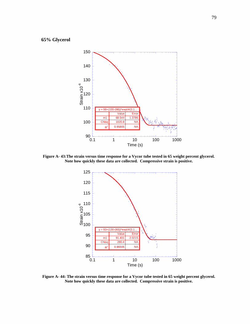
79

65% Glycerol

Figure A- 43:The strain versus time response for a Vycor tube tested in 65 weight percent glycerol.

Note how quickly these data are collected. Compressive strain is positive.

Figure A- 44: The strain versus time response for a Vycor tube tested in 65 weight percent glycerol.


90

100

110

120

130

140

150

0.1 1 10 100 1000

Str

ain

x10

-6

Time (s)

y = 98+(155-(98))*exp(4/(3.1...

ErrorValue

1.378668.544m1

NA1020.8Chisq

NA0.95805R2

85

90

95

100

105

110

115

120

125

0.1 1 10 100 1000

Str

ain

x10

-6

Time (s)

y = 93+(130-(93))*exp(4/(3.1...

ErrorValue

2.021591.401m1

NA280.4Chisq

NA0.96505R2

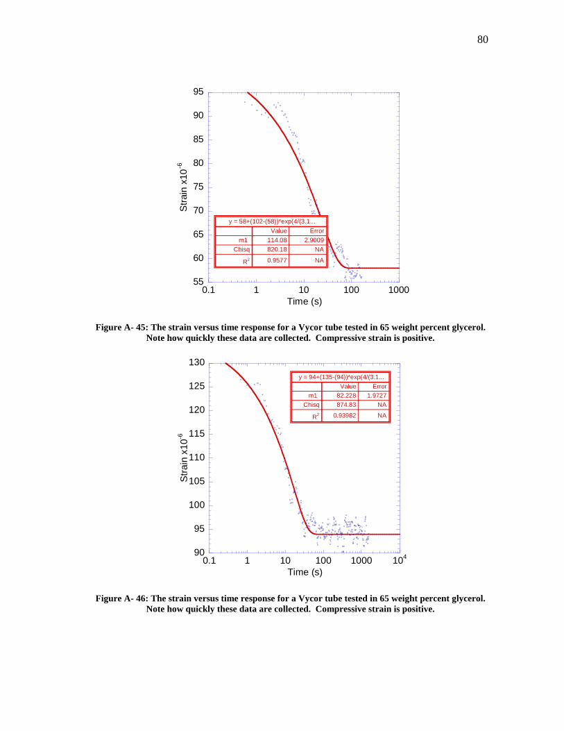
80





55

60

65

70

75

80

85

90

95

0.1 1 10 100 1000

Str

ain

x10

-6

Time (s)

y = 58+(102-(58))*exp(4/(3.1...

ErrorValue

2.9009114.08m1

NA820.18Chisq

NA0.9577R2

90

95

100

105

110

115

120

125

130

0.1 1 10 100 1000 104

Str

ain

x1

0-6

Time (s)

y = 94+(135-(94))*exp(4/(3.1...

ErrorValue

1.972782.228m1

NA874.83Chisq

NA0.93982R2

81





80

85

90

95

100

105

110

115

120

0.1 1 10 100 1000

Str

ain

x10

-6

Time (s)

y = 90+(131-(90))*exp(4/(3.1...

ErrorValue

2.057477.14m1

NA582.21Chisq

NA0.94906R2

85

90

95

100

105

110

115

120

125

0.1 1 10 100 1000

Str

ain

x10

-6

Time (s)

y = 92+(131-(92))*exp(4/(3.1...

ErrorValue

1.706173.229m1

NA279.94Chisq

NA0.96778R2

82





85

90

95

100

105

110

115

120

125

0.1 1 10 100 1000

Str

ain

x10

-6

Time (s)

y = 92+(133-(92))*exp(4/(3.1...

ErrorValue

2.162381.115m1

NA430.15Chisq

NA0.95639R2

100

110

120

130

140

150

0.1 1 10 100 1000

Str

ain

x1

0-6

Time (s)

y = 108+(155-(108))*exp(4/(3...

ErrorValue

2.590893.761m1

NA1180.1Chisq

NA0.9329R2

83





110

115

120

125

130

135

140

145

150

0.1 1 10 100 1000

Str

ain

x10

-6

Time (s)

y = 118+(156-(118))*exp(4/(3...

ErrorValue

2.614784.411m1

NA892.89Chisq

NA0.91713R2

90

95

100

105

110

115

120

125

130

0.1 1 10 100 1000

Str

ain

x10

-6

Time (s)

y = 96+(135-(96))*exp(4/(3.1...

ErrorValue

2.359377.951m1

NA812.52Chisq

NA0.94092R2

84

Vycor Solid Dynamic Pressurization Plots

100% Glycerol

Figure A- 53: The strain versus time response for a Vycor rod tested in pure glycerol. Compressive

strain is positive.

210

220

230

240

250

260

270

0.1 1 10 100 1000 104

105

Str

ain

x1

0-6

Time (s)

y = 218+(262-(218))*exp(4/(3...

ErrorValue

553.9947284m1

NA462.61Chisq

NA0.98866R2

85


strain is positive.


strain is positive.

150

160

170

180

190

200

210

220

0.1 1 10 100 1000 104

105

Str

ain

x1

0-6

Time (s)

y = 160+(210-(160))*exp(4/(3...

ErrorValue

758.845279m1

NA776.08Chisq

NA0.98429R2

150

155

160

165

170

175

180

185

190

0.1 1 10 100 1000 104

105

Str

ain

x1

0-6

Time (s)

y = 155+(186-(155))*exp(4/(3...

ErrorValue

1334.168457m1

NA349.44Chisq

NA0.97203R2

86


strain is positive.


strain is positive.

350

400

450

500

0.1 1 10 100 1000 104

105

Str

ain

x1

0-6

Time (s)

y = 360+(487-(360))*exp(4/(3...

ErrorValue

1121.577785m1

NA7571.2Chisq

NA0.984R2

320

340

360

380

400

420

0.1 1 10 100 1000 104

105

Str

ain

x1

0-6

Time (s)

y = 340+(415-(340))*exp(4/(3...

ErrorValue

1388.164977m1

NA3690.8Chisq

NA0.97303R2

87


strain is positive.


strain is positive.

80

100

120

140

160

180

200

0.1 1 10 100 1000 104

105

Str

ain

x1

0-6

Time (s)

y = 105+(182-(105))*exp(4/(3...

ErrorValue

1123.253151m1

NA4193.7Chisq

NA0.97711R2

80

100

120

140

160

180

200

220

240

0.1 1 10 100 1000 104

105

Str

ain

x1

0-6

Time (s)

y = 105+(230-(105))*exp(4/(3...

ErrorValue

1075.265951m1

NA11531Chisq

NA0.97939R2

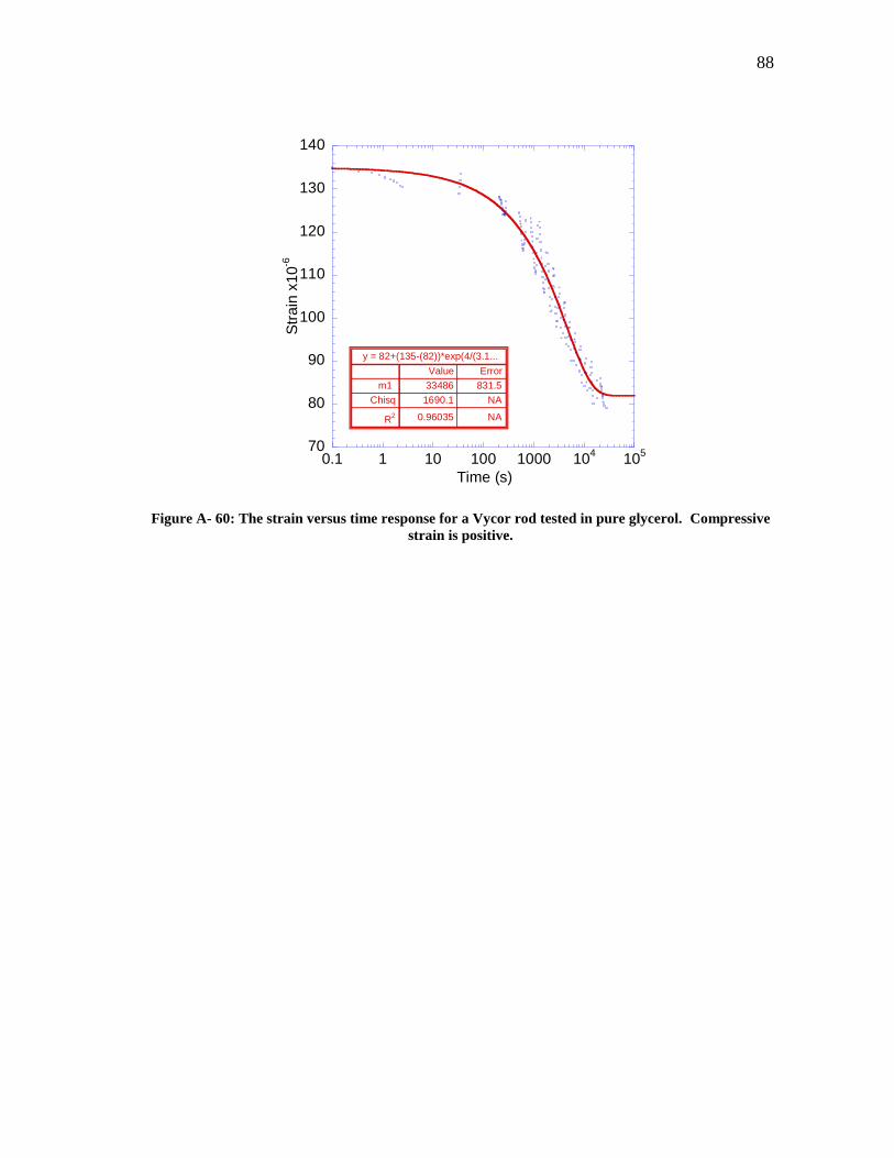
88


strain is positive.

70

80

90

100

110

120

130

140

0.1 1 10 100 1000 104

105

Str

ain

x1

0-6

Time (s)

y = 82+(135-(82))*exp(4/(3.1...

ErrorValue

831.533486m1

NA1690.1Chisq

NA0.96035R2

89

65% Glycerol

Figure A- 61: The strain versus time response for a Vycor rod tested in 65% glycerol. Compressive

strain is positive.

80

90

100

110

120

130

140

0.1 1 10 100 1000

Str

ain

x10

-6

Time (s)

y = 90+(133-(90))*exp(4/(3.1...

ErrorValue

17.017635.06m1

NA1143.2Chisq

NA0.95665R2

90


strain is positive.


strain is positive.

80

90

100

110

120

130

140

0.1 1 10 100 1000 104

Str

ain

x1

0-6

Time (s)

y = 90+(131-(90))*exp(4/(3.1...

ErrorValue

10.596488.7m1

NA1047.9Chisq

NA0.96933R2

80

90

100

110

120

130

140

0.1 1 10 100 1000 104

Str

ain

x1

0-6

Time (s)

y = 87+(130-(87))*exp(4/(3.1...

ErrorValue

10.965476.87m1

NA1329Chisq

NA0.96659R2

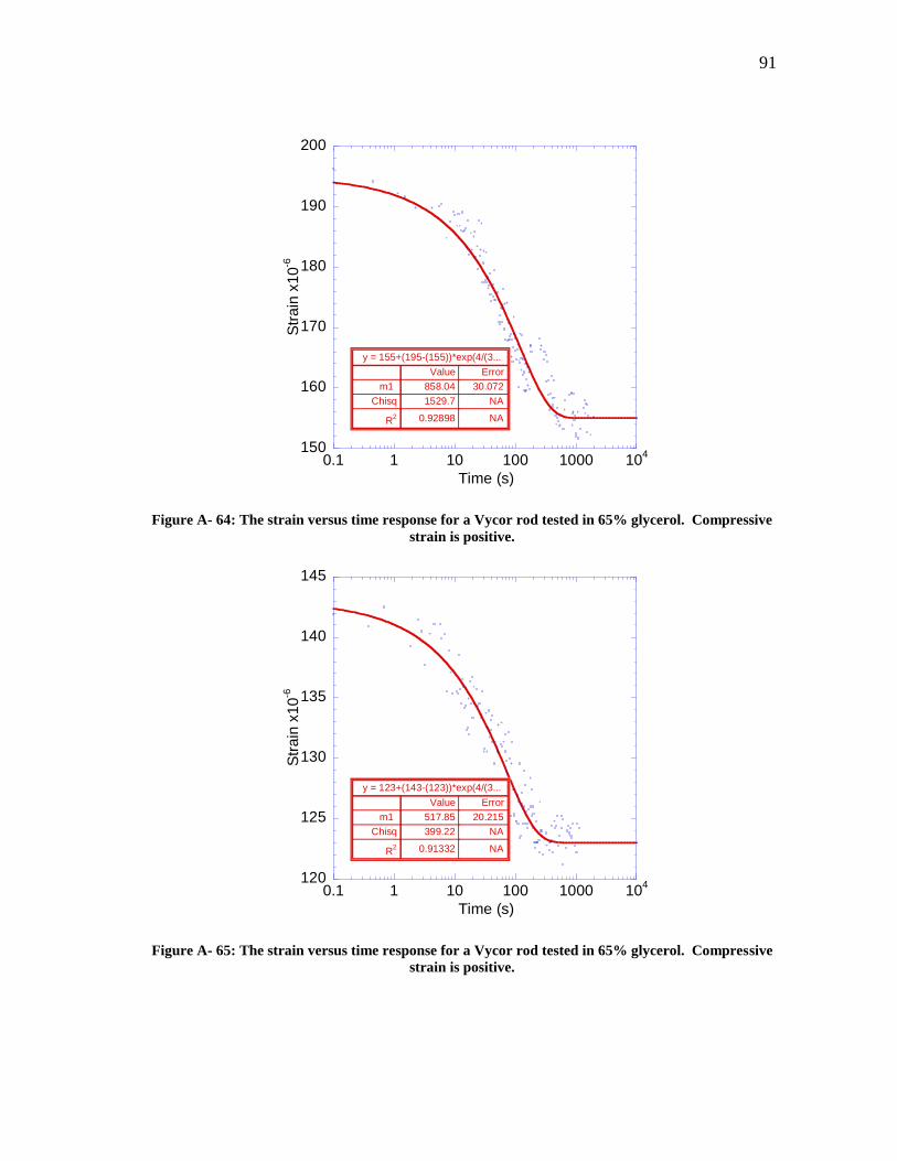
91


strain is positive.


strain is positive.

150

160

170

180

190

200

0.1 1 10 100 1000 104

Str

ain

x1

0-6

Time (s)

y = 155+(195-(155))*exp(4/(3...

ErrorValue

30.072858.04m1

NA1529.7Chisq

NA0.92898R2

120

125

130

135

140

145

0.1 1 10 100 1000 104

Str

ain

x1

0-6

Time (s)

y = 123+(143-(123))*exp(4/(3...

ErrorValue

20.215517.85m1

NA399.22Chisq

NA0.91332R2

92


strain is positive.


strain is positive.

120

140

160

180

200

220

0.1 1 10 100 1000 104

Str

ain

x1

0-6

Time (s)

y = 135+(203-(135))*exp(4/(3...

ErrorValue

30.1081364.2m1

NA2750.5Chisq

NA0.96888R2

120

130

140

150

160

170

180

190

200

0.1 1 10 100 1000 104

Str

ain

x1

0-6

Time (s)

y = 128+(195-(128))*exp(4/(3...

ErrorValue

27.0771516.3m1

NA1604.1Chisq

NA0.97725R2

93


strain is positive.


strain is positive.

130

140

150

160

170

180

190

200

210

0.1 1 10 100 1000 104

Str

ain

x1

0-6

Time (s)

y = 138+(209-(138))*exp(4/(3...

ErrorValue

19.2231153.6m1

NA1134.2Chisq

NA0.98405R2

120

140

160

180

200

220

0.1 1 10 100 1000

Str

ain

x10

-6

Time (s)

y = 130+(204-(130))*exp(4/(3...

ErrorValue

20.7121157.1m1

NA1836.8Chisq

NA0.97555R2

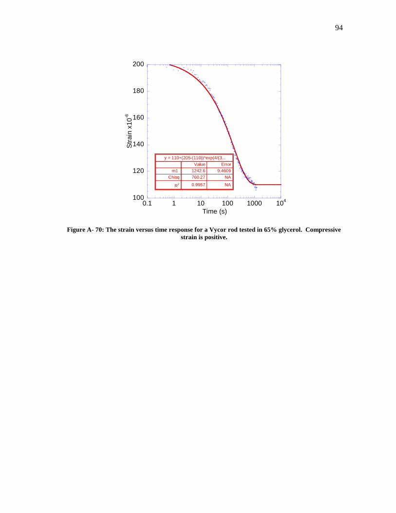
94


strain is positive.

100

120

140

160

180

200

0.1 1 10 100 1000 104

Str

ain

x1

0-6

Time (s)

y = 110+(205-(110))*exp(4/(3...

ErrorValue

9.46091242.6m1

NA760.27Chisq

NA0.9957R2

95

APPENDIX B. CEMENTITIOUS MATERIALS PLOTS

Cement Paste Flow Through Plots

Figure B- 1: The displacement versus time results for a 0.6 water to cement ratio specimen at an age

of 32 days and an applied pressure of 1.72 Mpa (250 psi). The testing fluid was water.

0

20

40

60

80

100

500 1000 1500 2000

y = -9.0124 + 0.052425x R2= 0.99177

Dis

pla

cem

en

t (I

nch

esx1

0-3

)

Time (s)

96





20

30

40

50

60

70

80

90

100

500 1000 1500 2000 2500

y = -21.773 + 0.05108x R2= 0.99706

Dis

pla

cem

en

t (I

nch

esx1

0-3

)

Time (s)

0

10

20

30

40

50

60

200 400 600 800 1000 1200

y = -1.4158 + 0.055462x R2= 0.99631

Dis

pla

cem

en

t (I

nch

esx1

0-3

)

Time (s)

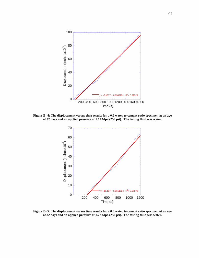
97





0

20

40

60

80

100

200 400 600 800 10001200140016001800

y = -3.1677 + 0.054775x R2= 0.99529

Dis

pla

cem

en

t (I

nch

esx1

0-3

)

Time (s)

0

10

20

30

40

50

60

70

200 400 600 800 1000 1200

y = -16.107 + 0.065162x R2= 0.98972

Dis

pla

cem

en

t (I

nch

esx1

0-3

)

Time (s)

98





0

20

40

60

80

100

500 1000 1500 2000

y = -6.1779 + 0.049109x R2= 0.99955

Dis

pla

cem

en

t (I

nch

esx1

0-3

)

Time (s)

0

20

40

60

80

100

200 400 600 800 10001200140016001800

y = -4.6161 + 0.053025x R2= 0.99527

Dis

pla

cem

en

t (I

nch

esx1

0-3

)

Time (s)

99





0

10

20

30

40

50

100 200 300 400 500 600 700 800

y = -3.9612 + 0.06401x R2= 0.99701

Dis

pla

cem

en

t (I

nch

esx1

0-3

)

Time (s)

0

20

40

60

80

100

500 1000 1500 2000 2500

y = -20.97 + 0.052976x R2= 0.95202

Dis

pla

cem

en

t (I

nch

esx1

0-3

)

Time (s)

100

Figure B- 10: The displacement versus time results for a 0.6 water to cement ratio specimen at an

age of 32 days and an applied pressure of 1.72 Mpa (250 psi). The testing fluid was water.



0

20

40

60

80

100

500 1000 1500 2000 2500

y = 2.8925 + 0.045777x R2= 0.98385

Dis

pla

ce

me

nt

(Inche

sx1

0-3

)

Time (s)

0

5

10

15

20

25

30

35

100 200 300 400 500 600 700

y = -0.91763 + 0.053004x R2= 0.99292

Dis

pla

cem

en

t (I

nch

esx1

0-3

)

Time (s)

101



0

5

10

15

20

25

30

35

40

100 200 300 400 500 600 700 800 900

y = -3.6731 + 0.046668x R2= 0.99711

Dis

pla

cem

en

t (I

nch

esx1

0-3

)

Time (s)

102

Cement Paste Hollow Dynamic Pressurization Plots

Figure B- 13: The strain versus time results for a 0.6 water to cement ratio specimen at an age of 33

days. The specimen was tested in water. Compressive strain is positive.



50

60

70

80

90

100

110

0.1 1 10 100 1000

Str

ain

x10

-6

Time (s)

y = 54+(105-(54))*exp(4/(3.1...

ErrorValue

19.753980.31m1

NA1845.6Chisq

NA0.96266R2

50

60

70

80

90

100

110

0.1 1 10 100 1000

Str

ain

x1

0-6

Time (s)

y = 54+(105-(54))*exp(4/(3.1...

ErrorValue

17.259980.41m1

NA1396.1Chisq

NA0.97074R2

103





40

50

60

70

80

90

100

110

120

0.1 1 10 100 1000 104

Str

ain

x1

0-6

Time (s)

y = 54+(110-(54))*exp(4/(3.1...

ErrorValue

22.852899.06m1

NA4264.4Chisq

NA0.94115R2

30

40

50

60

70

80

90

100

110

0.1 1 10 100 1000 104

Str

ain

x1

0-6

Time (s)

y = 40+(100-(40))*exp(4/(3.1...

ErrorValue

22.246803.95m1

NA5145.7Chisq

NA0.92039R2

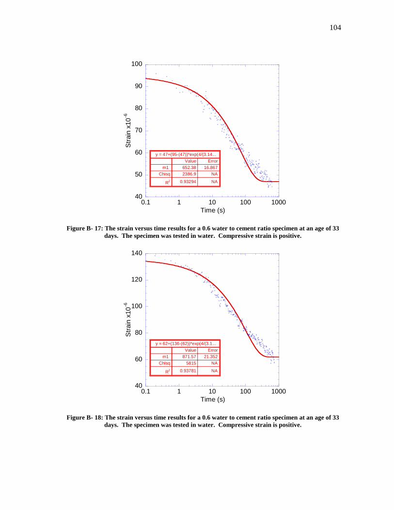
104





40

50

60

70

80

90

100

0.1 1 10 100 1000

Str

ain

x10

-6

Time (s)

y = 47+(95-(47))*exp(4/(3.14...

ErrorValue

16.867652.38m1

NA2386.9Chisq

NA0.93294R2

40

60

80

100

120

140

0.1 1 10 100 1000

Str

ain

x10

-6

Time (s)

y = 62+(136-(62))*exp(4/(3.1...

ErrorValue

21.352871.57m1

NA5815Chisq

NA0.93781R2

105





40

50

60

70

80

90

100

110

0.1 1 10 100 1000

Str

ain

x10

-6

Time (s)

y = 50+(105-(50))*exp(4/(3.1...

ErrorValue

18.268768.11m1

NA2867.8Chisq

NA0.94295R2

50

60

70

80

90

100

110

120

0.1 1 10 100 1000

Str

ain

x10

-6

Time (s)

y = 55+(115-(55))*exp(4/(3.1...

ErrorValue

18.314719.57m1

NA4081.8Chisq

NA0.93498R2

106





50

60

70

80

90

100

110

120

130

0.1 1 10 100 1000

Str

ain

x10

-6

Time (s)

y = 60+(125-(60))*exp(4/(3.1...

ErrorValue

13.791559.58m1

NA4541.6Chisq

NA0.94632R2

50

60

70

80

90

100

110

120

0.1 1 10 100 1000

Str

ain

x10

-6

Time (s)

y = 60+(115-(60))*exp(4/(3.1...

ErrorValue

15.792634.88m1

NA2230.6Chisq

NA0.93564R2

107


hours. The specimen was tested in water. Compressive strain is positive.



15

20

25

30

35

40

45

0.1 1 10 100 1000 104

Str

ain

x1

0-6

Time (s)

y = 18+(45-(18))*exp(4/(3.14...

ErrorValue

26.6921625.3m1

NA281.73Chisq

NA0.97982R2

0

20

40

60

80

100

0.1 1 10 100 1000 104

Str

ain

x1

0-6

Time (s)

y = 14+(90-(14))*exp(4/(3.14...

ErrorValue

75.1393827.5m1

NA2816.3Chisq

NA0.97306R2

108





0

5

10

15

20

25

30

35

0.1 1 10 100 1000 104

Str

ain

x1

0-6

Time (s)

y = 4+(33-(4))*exp(4/(3.1415...

ErrorValue

141.644911.9m1

NA495.99Chisq

NA0.95762R2

22

24

26

28

30

32

34

36

38

0.1 1 10 100 1000 104

Str

ain

x1

0-6

Time (s)

y = 20+(38-(20))*exp(4/(3.14...

ErrorValue

145.56289.7m1

NA188.75Chisq

NA0.95255R2

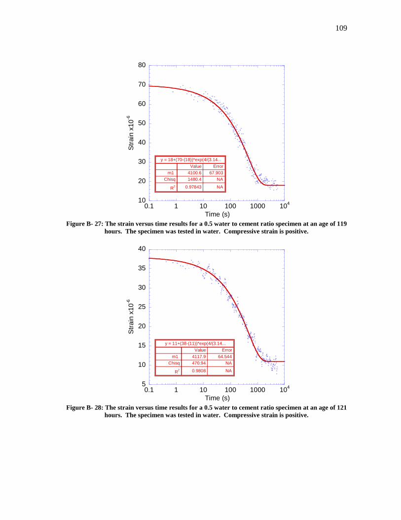
109





10

20

30

40

50

60

70

80

0.1 1 10 100 1000 104

Str

ain

x1

0-6

Time (s)

y = 18+(70-(18))*exp(4/(3.14...

ErrorValue

67.9034100.6m1

NA1480.4Chisq

NA0.97843R2

5

10

15

20

25

30

35

40

0.1 1 10 100 1000 104

Str

ain

x1

0-6

Time (s)

y = 11+(38-(11))*exp(4/(3.14...

ErrorValue

64.5444117.9m1

NA470.94Chisq

NA0.9808R2

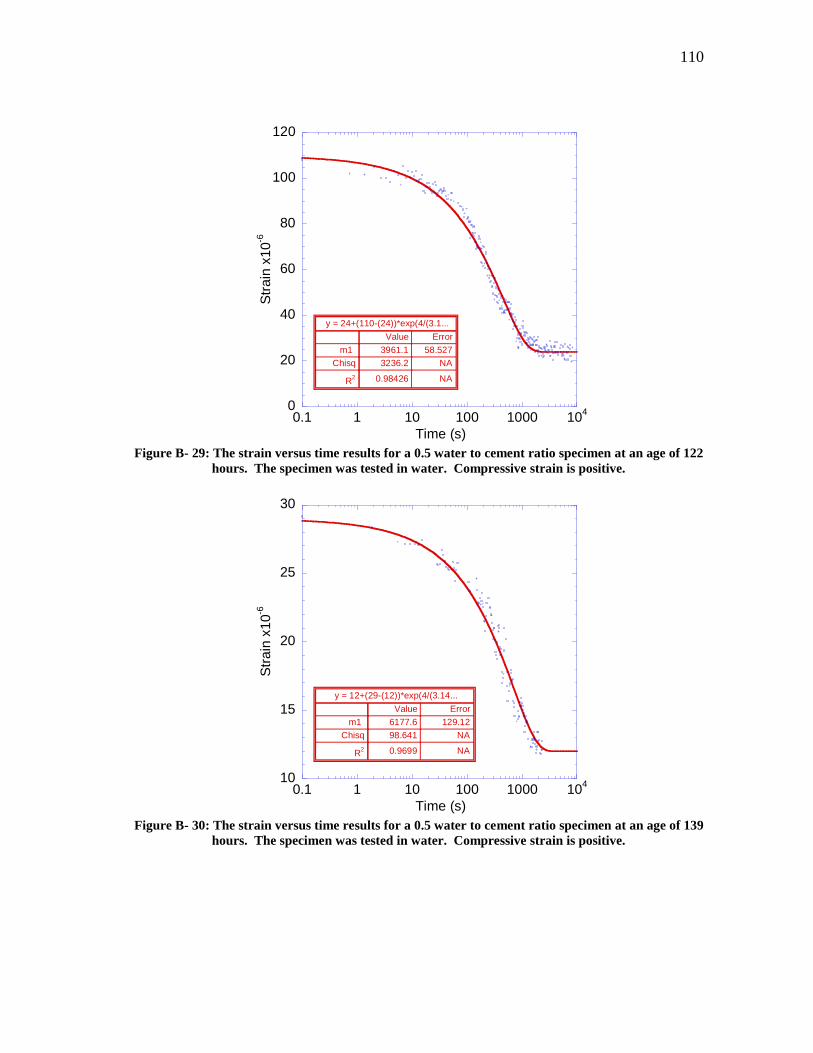
110





0

20

40

60

80

100

120

0.1 1 10 100 1000 104

Str

ain

x1

0-6

Time (s)

y = 24+(110-(24))*exp(4/(3.1...

ErrorValue

58.5273961.1m1

NA3236.2Chisq

NA0.98426R2

10

15

20

25

30

0.1 1 10 100 1000 104

Str

ain

x1

0-6

Time (s)

y = 12+(29-(12))*exp(4/(3.14...

ErrorValue

129.126177.6m1

NA98.641Chisq

NA0.9699R2

111





0

20

40

60

80

100

120

140

0.1 1 10 100 1000 104

Str

ain

x1

0-6

Time (s)

y = 22+(145-(22))*exp(4/(3.1...

ErrorValue

90.6445947.8m1

NA8192.4Chisq

NA0.98207R2

0

10

20

30

40

50

0.1 1 10 100 1000 104

Str

ain

x1

0-6

Time (s)

y = 9+(50-(9))*exp(4/(3.1415...

ErrorValue

164.119123.5m1

NA1090.2Chisq

NA0.9747R2

112





10

15

20

25

30

35

40

45

0.1 1 10 100 1000 104

Str

ain

x1

0-6

Time (s)

y = 14+(41-(14))*exp(4/(3.14...

ErrorValue

122.16190.1m1

NA437.76Chisq

NA0.97367R2

0

20

40

60

80

100

120

0.1 1 10 100 1000 104

Str

ain

x1

0-6

Time (s)

y = 22+(120-(22))*exp(4/(3.1...

ErrorValue

73.6455942.6m1

NA2581.8Chisq

NA0.98758R2

113





0

10

20

30

40

50

0.1 1 10 100 1000 104

Str

ain

x1

0-6

Time (s)

y = 10+(50-(10))*exp(4/(3.14...

ErrorValue

265.3311653m1

NA834.88Chisq

NA0.97042R2

10

20

30

40

50

60

0.1 1 10 100 1000 104

Str

ain

x1

0-6

Time (s)

y = 16+(58-(16))*exp(4/(3.14...

ErrorValue

115.125409m1

NA1050.8Chisq

NA0.96779R2

114





20

40

60

80

100

120

140

0.1 1 10 100 1000 104

105

Str

ain

x1

0-6

Time (s)

y = 28+(130-(28))*exp(4/(3.1...

ErrorValue

103.99003.6m1

NA2841.6Chisq

NA0.99R2

10

20

30

40

50

60

70

0.1 1 10 100 1000 104

105

Str

ain

x1

0-6

Time (s)

y = 18+(65-(18))*exp(4/(3.14...

ErrorValue

325.315535m1

NA1880.6Chisq

NA0.97092R2

115





5

10

15

20

25

30

35

40

45

0.1 1 10 100 1000 104

Str

ain

x1

0-6

Time (s)

y = 8+(44-(8))*exp(4/(3.1415...

ErrorValue

188.939679.9m1

NA854.15Chisq

NA0.97193R2

20

40

60

80

100

120

140

0.1 1 10 100 1000 104

105

Str

ain

x1

0-6

Time (s)

y = 35+(140-(35))*exp(4/(3.1...

ErrorValue

364.7925090m1

NA5724.9Chisq

NA0.98573R2

116





10

15

20

25

30

35

40

45

0.1 1 10 100 1000 104

Str

ain

x1

0-6

Time (s)

y = 14+(45-(14))*exp(4/(3.14...

ErrorValue

675.1323623m1

NA955.08Chisq

NA0.92548R2

20

40

60

80

100

120

140

0.1 1 10 100 1000 104

105

Str

ain

x1

0-6

Time (s)

y = 38+(135-(38))*exp(4/(3.1...

ErrorValue

432.227151m1

NA5509.8Chisq

NA0.98018R2

117





0

10

20

30

40

50

60

0.1 1 10 100 1000 104

105

Str

ain

x1

0-6

Time (s)

y = 10+(62-(10))*exp(4/(3.14...

ErrorValue

647.8723632m1

NA1454.9Chisq

NA0.95584R2

20

40

60

80

100

120

140

0.1 1 10 100 1000 104

105

Str

ain

x1

0-6

Time (s)

y = 28+(130-(28))*exp(4/(3.1...

ErrorValue

484.935103m1

NA4079Chisq

NA0.98305R2

118



10

20

30

40

50

60

70

0.1 1 10 100 1000 104

105

Str

ain

x1

0-6

Time (s)

y = 14+(60-(14))*exp(4/(3.14...

ErrorValue

1089.942805m1

NA1516.3Chisq

NA0.95624R2

119

Cement Paste Solid Dynamic Pressurization Plots



54

56

58

60

62

64

66

68

70

0.1 1 10 100 1000 104

Str

ain

x1

0-6

Time (s)

y = 55+(68-(55))*exp(4/(3.14...

ErrorValue

65.1933569.3m1

NA82.354Chisq

NA0.97424R2

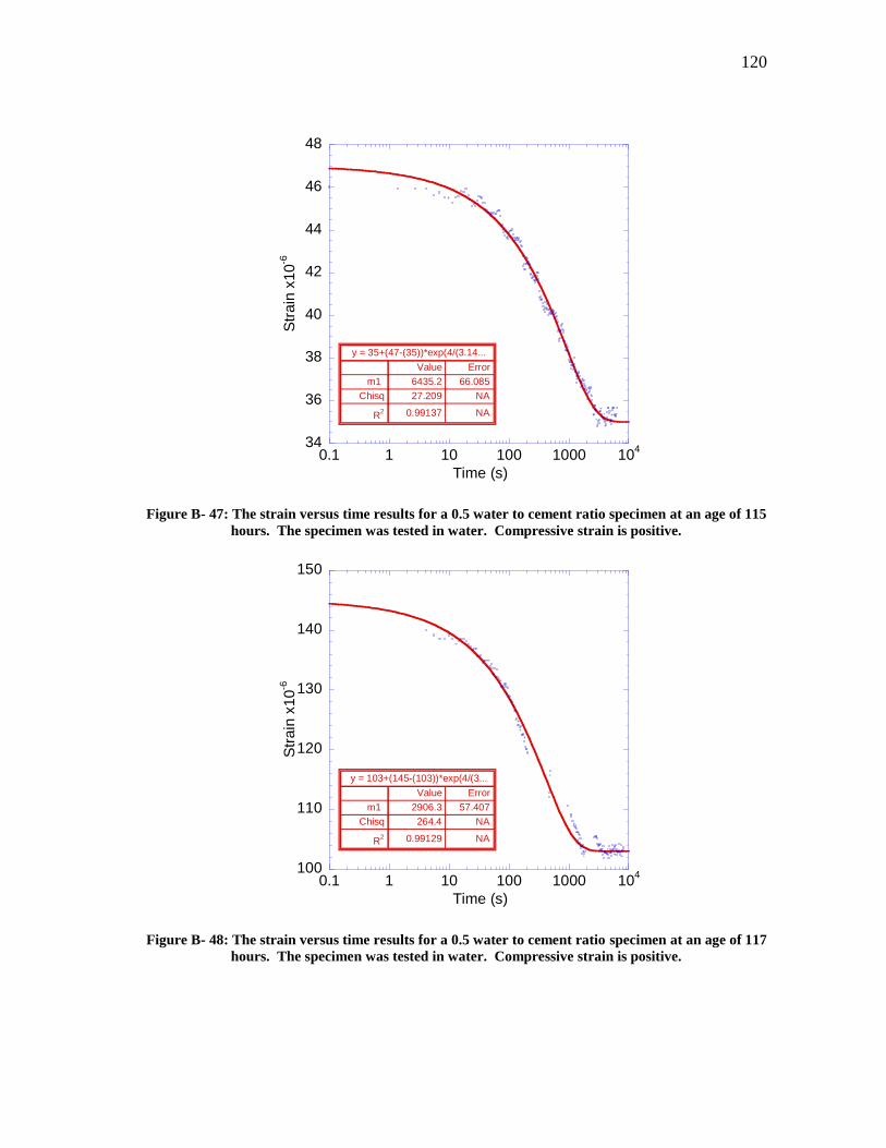
120





34

36

38

40

42

44

46

48

0.1 1 10 100 1000 104

Str

ain

x1

0-6

Time (s)

y = 35+(47-(35))*exp(4/(3.14...

ErrorValue

66.0856435.2m1

NA27.209Chisq

NA0.99137R2

100

110

120

130

140

150

0.1 1 10 100 1000 104

Str

ain

x1

0-6

Time (s)

y = 103+(145-(103))*exp(4/(3...

ErrorValue

57.4072906.3m1

NA264.4Chisq

NA0.99129R2

121





60

65

70

75

80

85

0.1 1 10 100 1000 104

Str

ain

x1

0-6

Time (s)

y = 65+(84-(65))*exp(4/(3.14...

ErrorValue

25.5541856.3m1

NA93.141Chisq

NA0.98417R2

75

80

85

90

95

100

105

110

0.1 1 10 100 1000 104

Str

ain

x1

0-6

Time (s)

y = 78+(110-(78))*exp(4/(3.1...

ErrorValue

19.4721893.8m1

NA167.64Chisq

NA0.9885R2

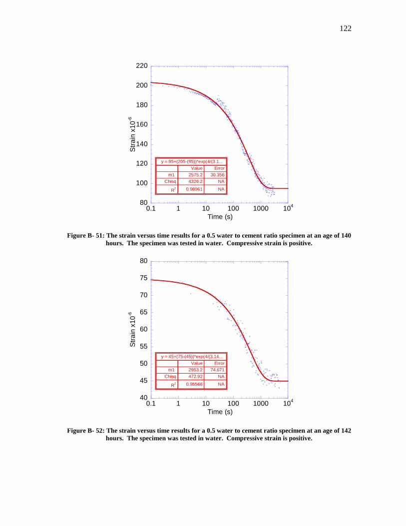
122





80

100

120

140

160

180

200

220

0.1 1 10 100 1000 104

Str

ain

x1

0-6

Time (s)

y = 95+(205-(95))*exp(4/(3.1...

ErrorValue

30.3562575.2m1

NA4326.2Chisq

NA0.98961R2

40

45

50

55

60

65

70

75

80

0.1 1 10 100 1000 104

Str

ain

x1

0-6

Time (s)

y = 45+(75-(45))*exp(4/(3.14...

ErrorValue

74.6712953.2m1

NA472.92Chisq

NA0.95566R2

123





80

100

120

140

160

180

200

220

0.1 1 10 100 1000 104

Str

ain

x1

0-6

Time (s)

y = 100+(200-(100))*exp(4/(3...

ErrorValue

51.5654178.9m1

NA4027.5Chisq

NA0.98967R2

40

50

60

70

80

90

100

0.1 1 10 100 1000 104

Str

ain

x1

0-6

Time (s)

y = 48+(96-(48))*exp(4/(3.14...

ErrorValue

32.651667.9m1

NA1445.3Chisq

NA0.97153R2

124





30

40

50

60

70

80

90

100

0.1 1 10 100 1000 104

105

Str

ain

x1

0-6

Time (s)

y = 38+(98-(38))*exp(4/(3.14...

ErrorValue

134.116273.8m1

NA3669.9Chisq

NA0.97286R2

100

120

140

160

180

200

220

0.1 1 10 100 1000 104

Str

ain

x1

0-6

Time (s)

y = 115+(217-(115))*exp(4/(3...

ErrorValue

47.3323744.6m1

NA3913.8Chisq

NA0.98818R2

125





50

60

70

80

90

100

110

120

0.1 1 10 100 1000 104

Str

ain

x1

0-6

Time (s)

y = 61+(116-(61))*exp(4/(3.1...

ErrorValue

35.7852170.6m1

NA1729.1Chisq

NA0.97994R2

30

40

50

60

70

80

0.1 1 10 100 1000 104

105

Str

ain

x1

0-6

Time (s)

y = 37+(78-(37))*exp(4/(3.14...

ErrorValue

135.035356.5m1

NA1417.9Chisq

NA0.9652R2

126





100

120

140

160

180

200

220

0.1 1 10 100 1000 104

105

Str

ain

x1

0-6

Time (s)

y = 110+(212-(110))*exp(4/(3...

ErrorValue

268.9515337m1

NA9042.7Chisq

NA0.97533R2

30

40

50

60

70

80

90

100

110

0.1 1 10 100 1000 104

105

Str

ain

x1

0-6

Time (s)

y = 38+(105-(38))*exp(4/(3.1...

ErrorValue

252.417693m1

NA2914.7Chisq

NA0.98652R2

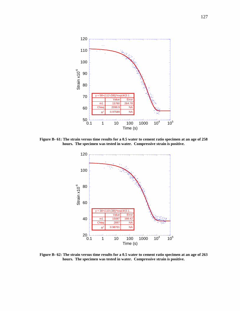
127





50

60

70

80

90

100

110

120

0.1 1 10 100 1000 104

105

Str

ain

x1

0-6

Time (s)

y = 58+(112-(58))*exp(4/(3.1...

ErrorValue

264.7815760m1

NA2099.9Chisq

NA0.97589R2

20

40

60

80

100

120

0.1 1 10 100 1000 104

105

Str

ain

x1

0-6

Time (s)

y = 38+(110-(38))*exp(4/(3.1...

ErrorValue

199.4215097m1

NA2897Chisq

NA0.98701R2

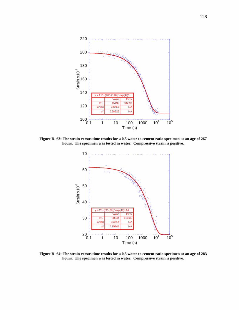
128





100

120

140

160

180

200

220

0.1 1 10 100 1000 104

105

Str

ain

x1

0-6

Time (s)

y = 110+(200-(110))*exp(4/(3...

ErrorValue

182.9715492m1

NA3293.6Chisq

NA0.98929R2

20

30

40

50

60

70

0.1 1 10 100 1000 104

105

Str

ain

x1

0-6

Time (s)

y = 20+(62-(20))*exp(4/(3.14...

ErrorValue

610.3230844m1

NA1592.4Chisq

NA0.95144R2

129





80

100

120

140

160

180

200

220

0.1 1 10 100 1000 104

105

Str

ain

x1

0-6

Time (s)

y = 105+(209-(105))*exp(4/(3...

ErrorValue

165.6215398m1

NA2934.8Chisq

NA0.99071R2

60

70

80

90

100

110

0.1 1 10 100 1000 104

105

Str

ain

x1

0-6

Time (s)

y = 66+(104-(66))*exp(4/(3.1...

ErrorValue

263.1412113m1

NA1605.7Chisq

NA0.96473R2

130

VITA

Christopher Andrew Jones was born in Corpus Christi, Texas. After graduating from

W.B. Ray High School in 2001, he enrolled in the 3-2 Dual Degree Engineering

Program at Southwestern University in Georgetown, Texas. Once he completed his

three years at Southwestern, Christopher enrolled as a student at Texas A&M University

in College Station, Texas where he graduated with a B.S. in civil engineering in

December of 2006. At this point Christopher was also awarded his B.A. in physical

science from Southwestern. While working on his master‟s degree Christopher was

supported by the Transportation Scholars Program through the Federal Highway

Administration. He will graduate with his Master of Science in August of 2008.

Christopher will continue at A&M and start work on his Ph.D.

Christopher A. Jones

8413 Alison Ave.

College Station, Texas 77845

HOLLOW CYLINDER DYNAMIC PRESSURIZATION AND RADIAL …

Documents

Transcript of HOLLOW CYLINDER DYNAMIC PRESSURIZATION AND RADIAL …