Holistic corpus-based dialectology - scielo.br · técnicas de análise multivariada (tais como...

561RBLA, Belo Horizonte, v. 11, n. 2, p. 561-592, 2011

* [email protected]

** [email protected]

Holistic corpus-based dialectologyDialetologia holística baseada em corpus

Benedikt Szmrecsanyi*Christoph Wolk**Freiburg Institute for Advanced StudiesFreiburg / Germany

ABSTRACT: This paper is concerned with sketching future directions for corpus-based dialectology. We advocate a holistic approach to the study of geographicallyconditioned linguistic variability, and we present a suitable methodology, ‘corpus-based dialectometry’, in exactly this spirit. Specifically, we argue that in order tolive up to the potential of the corpus-based method, practitioners need to (i)abandon their exclusive focus on individual linguistic features in favor of thestudy of feature aggregates, (ii) draw on computationally advanced multivariateanalysis techniques (such as multidimensional scaling, cluster analysis, and principalcomponent analysis), and (iii) aid interpretation of empirical results by marshallingstate-of-the-art data visualization techniques. To exemplify this line of analysis,we present a case study which explores joint frequency variability of 57morphosyntax features in 34 dialects all over Great Britain.KEYWORDS: corpus-based dialectology; holistic approach; corpus-baseddialectometry; feature aggregates; multivariate analysis; visualization techniques.

RESUMO: Este artigo debruça-se sobre o esboço propositivo de futuras direçõespara a dialetologia baseada em corpus. Defendemos uma abordagem holísticapara o estudo da variabilidade linguística geograficamente condicionada, eapresentamos uma metodologia adequada para tal – a dialetometria baseada emcorpus. Mais especificamente, defendemos que para que se obtenham todos osresultados esperados da metodologia de corpus, pesquisadores devem: (i) abandonarseu foco exclusivo em traços linguísticos individuais em favor do estudo dosagregados de traços, (ii) amparar-se em métodos computacionais avançados detécnicas de análise multivariada (tais como escalagem multidimensional, análise declusters, e análise de componente principal), e (iii) auxiliar a interpretação deresultados empíricos através da utilização do estado da arte em técnicas devisualização. A fim de exemplificarmos essa linha de análise, apresentamos umestudo de caso que explora a variabilidade da frequência agregada de 57 traçosmorfossintáticos de 34 dialetos da Grã-Bretanha.

PALAVRAS-CHAVE: dialetologia baseada em corpus; abordagem holística;dialetometria baseada em corpus; agregados de traços; análise multivariada; técnicasde visualização.

562 RBLA, Belo Horizonte, v. 11, n. 2, p. 561-592, 2011

1. Introduction

The customary data sources in traditional dialectology are dialectdictionaries, dialect atlases, and assorted other competence-centered materials.In the past couple of decades, however, more and more dialect corpora havebeen coming on-line, and corpus-linguistic methodologies have increasinglyfound their way into the dialectological toolbox (see ANDERWALD;SZMRECSANYI, 2009 for an overview). This is good news, for comparedto survey material corpora arguably yield a more realistic and performance-based linguistic signal. Yet, on the empirical-analytical plane corpus-basedapproaches to dialectology are still a far cry from the rigor and sophisticationcustomary in survey-based dialectology. This is particularly galling sincecorpora as a data type offer a host of exciting research opportunities notavailable otherwise. In this paper, we shall argue that corpus-baseddialectologists would be well advised to abandon their customary reliance onsingle-feature studies in favor of holistic, computational approaches thatexplore joint variability of feature aggregates. In short, we will be advocatinga methodology that we have referred to as CORPUS-BASED DIALECTOMETRY

(CBDM) elsewhere (cf. SZMRECSANYI, 2008; SZMRECSANYI, 2011).As a case study to explore CBDM’s analytical potential and to highlight the

benefits of holistic analysis, we shall tap the Freiburg Corpus of English Dialects(FRED) (HERNÁNDEZ, 2006; SZMRECSANYI; HERNÁNDEZ, 2007).FRED contains 368 individual texts and spans approximately 2.4 million wordsof running text, consisting of samples (mainly transcribed so-called ‘oralhistory’ material) of naturalistic, dialectal speech from a variety of sources.Most of these samples were recorded between 1970 and 1990; in most cases,a fieldworker interviewed an informant about life, work, etc. in former days.The 431 informants sampled in the corpus are typically elderly people witha working-class background. The interviews were conducted in 156 differentlocations (that is, villages and towns) in 34 different pre-1974 counties inGreat Britain including the Isle of Man and the Hebrides. The level of arealgranularity investigated in the present study will be the county level. This leavesus with 34 dialect objects that will be exemplarily subjected to dialectometricalanalysis in the subsequent sections.

This paper is structured as follows. In section 2, we present a numberof arguments in favor of holistic analysis. Section 3 defines corpus-baseddialectometry. Section 4 sketches some methodical preliminaries. Section 5draws on a measure of aggregate morphosyntactic distance to present a number


of ways in which dialectological datasets can be analyzed holistically:cartographic projections to geography (Section 5.1.), network diagrams(Section 5.2.), and correlational quantitative techniques (Section 5.3.). Section6 utilizes Principal Component Analysis to identify linguistic structure in thedataset. Section 7 offers some concluding remarks.

2. Holistic analysis – why?

AGGREGATE DATA ANALYSIS (also known as DATA SYNTHESIS) is concernednot with the distribution of individual features, properties, or measurements,but with the joint analysis of multiple characteristics. Aggregation is amethodical cornerstone in many academic disciplines. Taxonomists, forinstance, typically categorize species not on the basis of a single morphologicalor genetic criterion, but holistically on the basis of many. By contrast, inlinguistics and particularly in corpus linguistics, we find a long and stronglyentrenched tradition of looking at individual features in isolation, which ispartly a legacy of the discipline’s philological origins, and partly a convenienceissue. In any event, the one-feature-at-a-time line of analysis – exceptions suchas the multidimensional register studies in the spirit of Biber (1988)notwithstanding – has yielded a corpus-based dialectology literaturedominated by an abundance of what Nerbonne (2008) has referred to as‘single-feature-based studies’. We will refrain from citing actual studies here(but see the survey in ANDERWALD; SZMRECSANYI, 2009), thoughfictitious titles such as ‘Verbal complementation in West Yorkshire English’ or‘The KIT vowel in Appalachian English’ are entirely realistic. Now, single-featurestudies like this are completely fine, of course, when it is really the featuresthemselves (verbal complementation, the KIT vowel) that are of analyticinterest. The approach, however, is uninformative and, in fact, woefullyinadequate when single-feature analysts endeavor to characterize multidimensionalobjects such as dialects and the relationships between them, along the lines ofresearch questions such as ‘How does (the grammar and/or phonology and/or … of) Yorkshire English relate to (the grammar and/or phonology and/or… of) Appalachian English?’. In fact, for addressing questions like these the single-feature approach is about as uninformative and inadequate as a car comparison testwhose only criterion is, e.g., the number of cup holders installed.

The problem with single-feature studies – in dialectology as well aseverywhere else – is that feature selection is ultimately arbitrary (VIERECK,1985), and that the next feature down the road may or may not contradict the


characterization suggested by the previous feature. For example, YorkshireEnglish may be progressive in regard to verbal complementation, butconservative as far as verbal agreement is concerned. Thus, there is no guaranteethat some dialect or variety will exhibit the same distributional behavior inregard to different features. In addition, individual features may have fairlyspecific quirks to them that are irrelevant to the big picture and which create noise(NERBONNE, 2009). For instance, the KIT vowel in Appalachian Englishmay very well be a stark outlier in that dialect’s phonology, a possibility thatwe cannot rule out unless we proceed holistically and also look at other features.

In sum, we offer that holistic data analysis is indispensable whenever theanalyst’s attention is turned to the forest (‘dialects’), not the trees (‘dialectfeatures’). Data synthesis and aggregation mitigate the problem of feature-specific quirks, irrelevant statistical noise, and the problem of inherentlysubjective feature selection, and can thus unearth a more robust, objective, andrealistic linguistic signal.

3. Corpus-based dialectometry

The shortcomings of non-holistic analysis have been known since atleast the 1930s (cf., for example, BLOOMFIELD, 1984 [1933]: chapter 19).Starting in the 1970s, computationally inclined dialectologists have addressedthese worries by developing a methodology known as DIALECTOMETRY.Dialectometry is defined as the branch of geolinguistics concerned withmeasuring, visualizing, and analyzing aggregate dialect similarities or distancesas a function of properties of geographic space (for seminal work, see SÉGUY,1971; GOEBL, 1982; GOEBL, 1984; NERBONNE; HEERINGA;KLEIWEG, 1999; HEERINGA, 2004; NERBONNE, 2005; GOEBL,2006; NERBONNE; KLEIWEG, 2007). Dialectometrical inquiry marshalscomputational approaches to identify “general, seemingly hidden structuresfrom a larger amount of features” (GOEBL; SCHILTZ, 1997, p. 13) and putsa strong emphasis on quantification, cartographic visualization, andexploratory data analysis to infer patterns from feature aggregates.

Orthodox dialectometry relies on digitized dialect atlases as its primarydata source. By contrast, the present contribution outlines a variety ofdialectometry that we call CORPUS-BASED DIALECTOMETRY (henceforth: CBDM).The atlas-based method has undeniable advantages – in particular, a fairlywidespread availability of data sources and superb areal coverage. By contrast,dialect corpora are in somewhat shorter supply, and their areal coverage is


typically inferior to dialect atlases. Having said that, as a data source, corporahave interesting advantages over dialect atlases. First and foremost, the atlassignal is categorical, exhibits a high level of data reduction, and may hence beless accurate than the corpus signal, which can provide graded frequencyinformation. While the exact cognitive status of text frequencies is admittedlystill unclear – for example, we do not currently know about the precise extentto which corpus frequencies correlate with psychological entrenchment(ARPPE; GILQUIN; GLYNN; HILPERT; ZESCHEL, 2010) – we doclaim that text frequencies match better with the reality of the input perceivedby hearers than discrete atlas classifications. Second, we note that the atlas signalis non-naturalistic and, basically, meta-linguistic in nature. It typically relieson elicitation and questionnaires, and is analytically twice removed (viafieldworkers and atlas compilers) from the analyst. By contrast, text corpora– and, by extension, CBDM – provide more direct access to language form andfunction, and may thus yield a more realistic and trustworthy picture.Furthermore, corpus material is more easily extensible in two ways. On theone hand, it is easier to supplement corpus databases with additional material;for example, oral history recordings comparable to the ones used in FRED areeasier to come by than informants that are equally comparable to the ones thatcompleted some atlas questionnaire decades ago. On the other hand, theanalysis of atlas data is constrained by the design of the questionnaire, allowingonly in a limited way for the study of research questions not originallyenvisaged. The corpus-based analyst, by contrast, is at more liberty to approachnew questions, given that the corpus is of sufficient size.

The well-known major intrinsic drawback of the corpus-based methodis that it is unable to deal with textually infrequent phenomena (see, e.g.,PENKE; ROSENBACH, 2004, p. 489), and data sparsity is a particular concernwhen the focus is on syntax and lexis; in this case, a questionnaire study mayindeed be the more appropriate research design. Nonetheless, one mayjustifiably wonder if phenomena that are so infrequent that they cannot bedescribed on the basis of a major text corpus should have a place in an aggregateanalysis at all.

4. Methodical preliminaries

The first step in CBDM calls for defining the feature catalogue as theempirical basis for the data synthesis endeavor. In keeping true to the spirit ofdialectometrical analysis and for the sake of avoiding the subjectivity inherent


in feature selection, the goal is to base the analysis on as many features aspossible. In the case study at hand, we surveyed the dialectological, variationist,and corpus-linguistic literature on morphosyntactic variability in varieties ofEnglish for suitable phenomena. This resulted in a list of p = 57 features, whichoverlaps with but is not identical to recent comparative English morphosyntaxsurveys (cf. KORTMANN; SZMRECSANYI, 2004; SZMRECSANYI;KORTMANN, 2009) and the battery of morphosyntax features covered inthe Survey of English Dialects (for example, ORTON; SANDERSON;WIDDOWSON, 1978). The Appendix lists the features in the catalogue; fora detailed discussion of the selection criteria, the reader is referred toSzmrecsanyi (2011).

Next, the analyst extracts feature frequencies from the corpus accordingto best corpus linguistic practice. Szmrecsanyi (2010) details the technicalitiesof the extraction process in terms of our CBDM case study. Once featurefrequencies are extracted, the analyst will normalize text frequencies, andpossibly apply a log-transformation to de-emphasize large frequencydifferentials and to alleviate the effect of frequency outliers. Lastly, an N × pfrequency matrix is created in which the N objects (that is, dialects or varieties)are arranged in rows and the p features in columns, such that each cell in thematrix specifies a particular (normalized and log-transformed) featurefrequency. Our CBDM case study thus yields a 34 × 57 frequency matrix: 34British English dialects, each characterized by a vector of 57 (normalized andlog-transformed) text frequencies. The matrix yields a Cronbach’s a (cf.NUNNALLY, 1978) value of .77, a score that indicates acceptable reliability.

5. Analyzing dialect relationships in the aggregate perspective

The first line of holistic analysis that we shall explore in this paperconverts an N × p frequency matrix into an N × N distance matrix. Thistransformation is radically aggregational, in that the resulting distance matrixabstracts away from individual feature frequencies and specifies pairwisedistances between the objects. Given the continuous nature of corpus-derivedfrequency vectors, we advocate usage of the well-known and fairlystraightforward Euclidean distance measure (ALDENDERFER;BLASHFIELD, 1984, p. 25), which is also known as ‘ruler distance’. Basedon the Pythagorean theorem, the measure defines the distance between twodialect objects a and b as the square root of the sum of all p squared frequencydifferentials:


where p is the number of features, a1 is the frequency of feature 1 in object a,

b1 is the frequency of feature 1 in object b, a

2 is the frequency of feature 2 in

object a, and so on.

The chart in Figure 1 illustrates the aggregation process. In step , westart out with a fictional 3 × 2 frequency matrix, which has 6 cells specifyingfrequencies of 2 features in 3 dialects. In step we calculate three distances:the distance between dialects a and b (which we commonsensically define asidentical to the distance between dialects b and a), the distance between dialectsa and c, and the distance between dialects b and c. In step , we enter thesedistances into a 3 × 3 distance matrix.

Distance matrices can be analyzed in a myriad ways – numerically,cartographically, and diagrammatically. Our cbdm case study’s 34 × 57frequency matrix yields a 34 × 34 distance matrix which describes 34 × 33/2= 561 pairwise distances between the dialect objects under study. The meanmorphosyntactic distance is 5.41 Euclidean distance points. As for the dataset-internal dispersion around the mean, we are dealing with a standard deviationof 1.11. This is another way of saying that roughly two thirds of the 561 dialectpairings score a distance within 1.11 points of the mean, and that 95% of allpairwise distances do not deviate more than 2.22 points from the mean. Theminimum observable distance in the dataset is 2.32 points (this happens to

1

2

3


be the morphosyntactic distance between the dialects spoken in the county ofSomerset and the county of Wiltshire, two neighboring counties located inthe Southwest of England). The maximum observable distance in the datasetis 8.14 points, which is the distance between the dialects spoken in the countyof Denbighshire in Wales and the county of Kincardineshire in the ScottishLowlands. The distance matrix comes with a skewness value of -.06, whichindicates a very slight negative skew. The kurtosis value is -.37, which isanother way of saying that the distribution of distances is a bit flatter than itwould be in a perfectly normal distribution.

5.1. Cartography

This section will introduce three fairly customary map types that canbe utilized to project (aspects of ) the information provided in distancematrices to geography: beam maps, continuum maps, and cluster maps. Ona technical note, all maps presented in this section were created using freelyavailable dialectometry software: the Visual DialectoMetry (VDM) packagedeveloped in Salzburg (HAIMERL, 2006), and the Groningen linguist PeterKleiweg’s RuG/L04 dialectometry software package (available online at <http://www.let.rug.nl/~kleiweg/L04/>).


5.1.1. Beam maps

MAP 1. Beam map. Morphosyntactically distant neighbors are connected by cold and thinbeams; neighbors that are close morphosyntactically are connected by warm and heavy beams


Beam maps are comparatively straightforward maps that project distancematrices to geography without much statistical ado. They are easy to readbecause the map type restricts attention to so-called ‘interpoint’ (i.e. neighbor)relationships (GOEBL, 1982, p. 51). In this spirit, we now turn to Map 1, whichfeatures a beam map visually depicting interpoint relationships in our 34 × 34distance matrix. As for the color coding, note that morphosyntactically distantneighbors are connected by cold (blueish) and thin beams; neighbors that areclose morphosyntactically are connected by warm (reddish) and heavy beams.Visual inspection of Map 1 suggests four hotbeds of neighborly similarity inGreat Britain. These highlight a very crucial dialect division well-known fromthe literature – the split between dialects spoken (i) in the Southwest ofEngland, (ii) dialects spoken in the Southeast of England, (iii) dialects spokenin the North of England, and (iv) Scots dialects:

• In the Southwest of England, there is a comparatively marked axis ofinterpoint similarities running from Cornwall via Devon and Somersetall the way to Wiltshire.

• In the Southeast of England, we note a triangle of relatively modestmorphosyntactic similarities connecting Kent, London, and Suffolk.

• In the Northern Midlands and the North of England, we find a webof strong interpoint similarities encompassing Nottinghamshire,Lancashire, Westmorland, Yorkshire, and Durham.

• The Central Scottish Lowlands exhibit a bolt of interpoint similaritiesinvolving parts of the urbanized ‘Central Belt’.

5.1.2. Continuum maps

Many geolinguists intuitively assume that geographic proximitypredicts dialectal similarity (cf. NERBONNE; KLEIWEG, 2007, p. 154).This section utilizes more advanced cartography – specifically, so-calledcontinuum maps (HEERINGA, 2004) – to map the extent to whichlinguistic distance is directly proportional to geographic distance such thatthere are “no real boundaries, but only gradual transitions” (BLOOMFIELD,1984 [1933], p. 341). We set the scene by utilizing customary Voronoitesselation (VORONOI, 1907) to assign each dialect site on the map a convexpolygon such that each point within the polygon is closer to the generatingdialect site than to any other dialect site (note that as our CBDM case studycovers Great Britain with just N = 34 sampling points, we will prefer to limit


the radius of the Voronoi polygons to approximately 50km in order to dovisual justice to the areal coverage of the dialect corpus). The next step is acomputational one and subjects the 34 × 34 distance matrix toMultidimensional Scaling (MDS) (KRUSKAL; WISH, 1978; EMBLETON,1993), an exploratory statistical technique to reduce a higher-dimensionaldataset to a lower-dimensional representation which is more amenable tovisualization. We thus scale down our high-dimensional distance matrix to athree-dimensional representation, in which each object (i.e. dialect) has acoordinate in three artificial MDS dimensions. These coordinates are thenmapped to the red-green-blue color scheme, giving each of the Voronoipolygons a distinct hue. Interpetationally, smooth color transitions betweendialect polygons emphasize the continuum-like nature of the dialectlandscape; abrupt color transitions point to the necessity of alternativeexplanations.

MAP 2. Continuum similarity. Correlation with distances in the original distance matrix:r = .95. Map labels are three-letter Chapman county codes

(see <http://www.genuki.org.uk/big/Regions/Codes.html> for a legend)


Consider, now, the continuum map in Map 2. The MDS solution depicted isa very accurate one, in that the distances in the three artificial MDS dimensionscorrelate highly (r = .95) with the distances in the original 34 × 34 distancematrix. In all, the mosaic pattern in the continuum map suggests that themorphosyntactic dialect landscape in Great Britain is in all not exceedinglycontinuum-like. For sure, there are some fairly nice micro-continua (in, say,the Southwest of England and in the Central and Northern ScottishLowlands); notice also how nicely dialects spoken in the North of Englandfade into Southern Scottish Lowlands dialects. But we also observe ratherabrupt transitions, for example between the Central Scottish Lowlands andSouthern Scottish dialects (Peebleshire and Selkirkshire). In England, thedialects spoken in Middlesex and Warwickshire are outliers. In Wales, it isDenbighshire that does not fit into the picture.

5.1.3. Cluster maps

The assumption guiding the discussion in the previous section was thatlinguistic similarity between dialects is inversely proportional to geographicdistance between dialects, and we have seen that this assumption does notnecessarily mesh well with the empirical facts. There is, however, an alternativeview, according to which dialect landscapes may be geographically organizedalong the lines of geographically cohesive and linguistically homogeneous “areaswithin which similar varieties are spoken” (HEERINGA; NERBONNE,2001, p. 375).


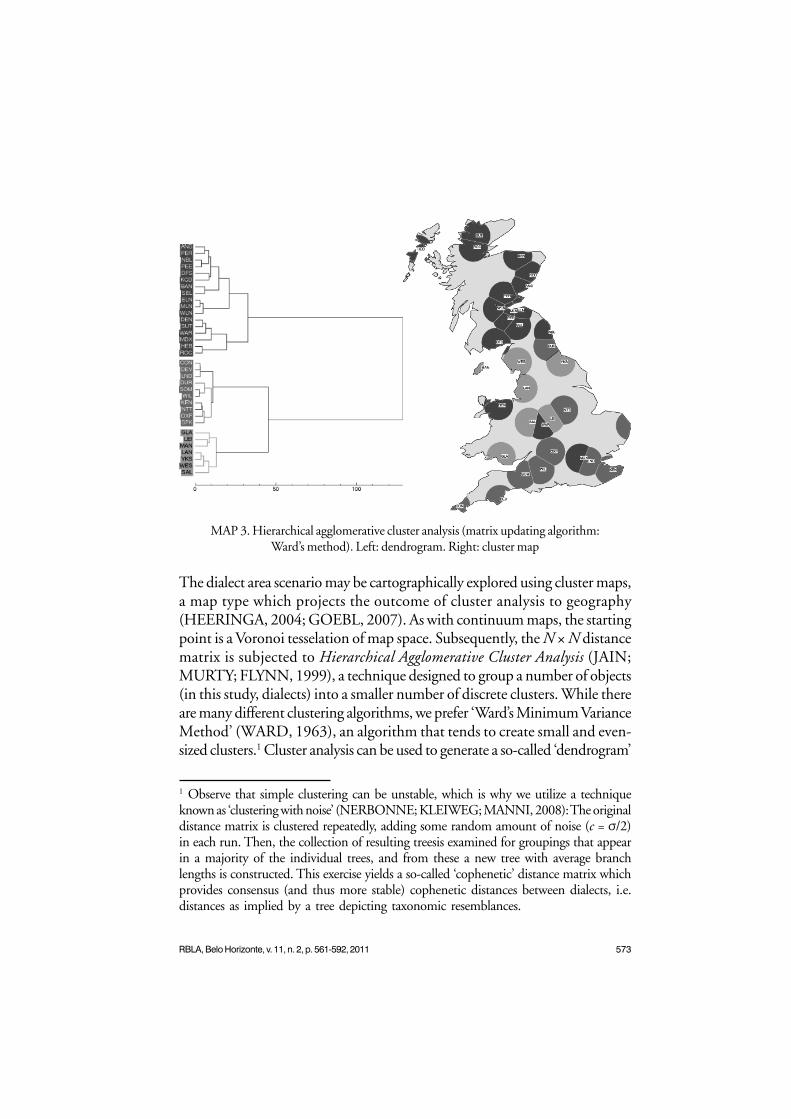
MAP 3. Hierarchical agglomerative cluster analysis (matrix updating algorithm:Ward’s method). Left: dendrogram. Right: cluster map

The dialect area scenario may be cartographically explored using cluster maps,a map type which projects the outcome of cluster analysis to geography(HEERINGA, 2004; GOEBL, 2007). As with continuum maps, the startingpoint is a Voronoi tesselation of map space. Subsequently, the N × N distancematrix is subjected to Hierarchical Agglomerative Cluster Analysis (JAIN;MURTY; FLYNN, 1999), a technique designed to group a number of objects(in this study, dialects) into a smaller number of discrete clusters. While thereare many different clustering algorithms, we prefer ‘Ward’s Minimum VarianceMethod’ (WARD, 1963), an algorithm that tends to create small and even-sized clusters.1 Cluster analysis can be used to generate a so-called ‘dendrogram’

1 Observe that simple clustering can be unstable, which is why we utilize a techniqueknown as ‘clustering with noise’ (NERBONNE; KLEIWEG; MANNI, 2008): The originaldistance matrix is clustered repeatedly, adding some random amount of noise (c = s/2)in each run. Then, the collection of resulting treesis examined for groupings that appearin a majority of the individual trees, and from these a new tree with average branchlengths is constructed. This exercise yields a so-called ‘cophenetic’ distance matrix whichprovides consensus (and thus more stable) cophenetic distances between dialects, i.e.distances as implied by a tree depicting taxonomic resemblances.


(cf. Map 3), which depicts cophenetic distances between the clustered objects.The optimal number of clusters can be determined by ‘elbowing’, i.e.diagramming the number of clusters against the fusion coefficient and spottingthe ‘elbow’ in the resulting graph (ALDENDERFER; BLASHFIELD, 1984,p. 54). Finally, each of the clusters is assigned a distinct color hue and theVoronoi polygons are colorized accordingly. Map 3 projects clusters in ourCBDM dataset to geography. Despite some geographic incoherence, clusteranalysis does detect an areal pattern:

• We find a geographically modestly coherent red cluster comprisingmost Southern English measuring points (Middlesex being theexception) plus Nottinghamshire in Central England, Suffolk in EastAnglia, and Durham in Northern England.

• We also obtain a geographically fairly coherent green group encompassingthe majority of measuring points in Northern England (Westmorland,Yorkshire, Lancashire), the Isle of Man, Shropshire and Leicestershirein Central England, and Glamorganshire in Southern Wales.

• Lastly, we are faced with a blue mixed-bag cluster uniting all measuringpoints in Scotland plus Northumberland in Northern England plusDenbighshire in Northern Wales plus Warwickshire in Central Englandplus Middlesex in Southern England.

5.2. Network diagrams

The previous section introduced agglomerative clustering as aclassification method based on dissimilarity, and dendrograms as one way ofvisualizing its results. Many variants of this general approach have beendeveloped, most of which yield a strictly hierarchical output. Theirrepresentation of sub-cluster structure allows interpretation in terms ofdiachronic development, which is used to great effect in bioinformatics forinferring evolutionary history. In that field, the need to represent uncertaintyin the resulting phylogenies as well as mixed evolutionary paths resulting fromreticulate effects such as genetic recombination has led to the development of‘splits graphs’ for representing non-hierarchical classification (DRESS;HUSON, 2004). One method for constructing such networks, NeighborNet(BRYANT; MOULTON, 2004), has found a following in linguistics forhistorical (McMAHON; McMAHON, 2005), dialectological (McMAHON;HEGGARTY; McMAHON; MAGUIRE, 2007), and typological (CYSOUW,


2007) purposes, thanks to NeighborNet’s ability to detect conflicting signalsand to represent the effects of language contact. The majority of currentapplications of NeighborNet in linguistics are restricted to the analysis ofcategorical atlas-type data. In this section we seek to sketch some of thepromises the technique holds for frequency-based analyses.

Let us begin by briefly sketching the algorithm that generates thenetwork diagrams. NeighborNet has the same starting point as the previousanalyses – a distance matrix.2 As with hierarchical agglomerative cluster analysis,the distance matrix is searched for the pair of points with the shortest distance.Instead of immediately fusing these points to a single cluster, however, theyare just marked, and this procedure is repeated until the same point is markedtwice. Then, these points are replaced with two clusters, each representing thedoubly marked point in relation to one of its marked neighbors. This processis repeated until only three clusters are left. The fusion sequence cansubsequently be used to generate a network-like diagram. This procedure hassome beneficial properties. First, the result will not be needlessly complex. Forcases where a segment of the data can be adequately represented as a hierarchicaltree, the corresponding segment of the network will be tree-shaped. Second,the method will always produce graphs that are planar, i.e. without crossinglines, which aids visual interpretation.

Figure 2 depicts a network based on the FRED 34 × 34 distance matrix;broad a priori dialect areas are indicated via colored labels. The graph was createdusing the freely available SplitsTree package (HUSON; BRYANT, 2006).When interpreting such networks, the equivalents of edges connecting twotree nodes in a dendrogram are either individual lines, or sets of parallel lines.In this network, we only find individual lines directly at the leaf nodes, andmany sets of parallel lines, combining to the boxy shapes that form the bodyof the network. Each represents a way of splitting the total set of dialects intoexactly two groups. The longer a given line or set of lines, the greater thedifference between the groups. To give an example, the comparatively large verticalset of lines directly below the point where Durham joins the network divides thedialects into the following two groups: one group that consists of Nottinghamshireas well as all Southwestern and Southeastern dialects except Middlesex, andanother group that contains all other dialects. When two such divisions are not

2 On a technical note, NeighborNet relies on observed distances to create a newmatrix which takes the net divergences of the involved objects into account.


representable as strictly hierarchical, the resulting lines form boxy shapes.Comparing the network to the strict clustering provided by the dendrogram inMap 3, we find that the network shows considerable amounts of incompatiblegroupings, indicating that a simple hierarchical classification structure does notentirely adequately capture the uncertainty present in the data.

FIGURE 2. Network representation of morphosyntactic distances.Colors indicate a priori dialect areas.

We now turn to the actual networks presented in Figure 2. Overall, thematch between dialect areas and placement along the graph seems quite good,as there are several regions on the graph that map to large-scale geographic areas:most Southern dialects can be found at the lower end of the diagram,


progressing clockwise through Midlands and Northern dialects toward theScottish dialects at the top. Most of the non-Scottish components of the‘mixed-bag’ cluster discussed in Section 5.1.3., as well as the ScottishHighlands and the Hebrides, are distributed along the right-hand side. Thecorrespondence between geography and the network is certainly not perfect,as some distinctions – such as the difference between Southeastern andSouthwestern English dialects – do not materialize in the graph, and theMidlands are mostly intermingled with either Southern or Northern Englishdialects. Closer inspection of the individual groupings shows that while someof the large-scale areas, such as the (mostly) Southern group mentioned above,are actually represented by an individual split, others (such as the North ofEngland) are not really a single group, but a collection of smaller ones withinterlocking resemblances. As one moves from the center of the networktoward the individual dialects, such structure becomes apparent throughoutthe graph, and it is here where the advantage of networks over treerepresentations is easiest to see. For example, the sub-tree of the dendrogramin Map 3 that connects the rather central Oxfordshire to Nottinghamshire,Kent and Suffolk is still present in the network. Nonetheless, there is also anew, incompatible grouping of Oxfordshire with Devon to the West. Thissuggests that individual similarities in both directions exist, beyond those thatcan be explained by the fact that each is a member of the group of (mostly)Southern English dialects. A similar case can be found in the ScottishLowlands, where the measuring points East Lothian and Midlothian form arather treelike subgroup. West Lothian, by contrast, is notably removedtoward the northern Lowlands. Again, a geographic interpretation is possible,as West Lothian is closer to the northern areas by land and the fjord that separatesthem from the Lothians, the Firth of Forth, widens considerably to its east.

Network representations are well-suited for finding such suggestivepatterns. Compared to the other methods presented in the current paper,though, they are still rather new – especially as applied to dialectological data– and we anticipate future scholarship to further enhance their interpretationalutility in the realm of (corpus-based) geolinguistics. Fruitful topics may includecontext-appropriate validation techniques to increase classification stability ina principled way, projection of non-hierarchical clusters to geography, andtechniques for folding network structures back on the individual features fromwhich they originate.


5.3. Quantifying the effect of language-external predictors

CBDM is intrinsically quantitative, yet it is fair to say that the foregoingdiscussion has relied heavily on interpreting cartographic projections togeography and other diagrammatic representations. However, the analyst mayalso correlate language-external parameters with linguistic distances to preciselyquantify the extent to which dialect distances are predictable from language-external factors in the aggregate perspective. Starting out with an N × Nlinguistic distance matrix, the name of the game is creating parallel language-external distance matrices, one for each predictor to be tested. In the simplestcase, each of these language-external distance matrices is then correlated withthe linguistic distance matrix by calculating, e.g., a Pearson product-momentcorrelation coefficient. The language-external predictor that scores the highestcoefficient is the best predictor of linguistic distances (more sophisticatedresearch designs may marshal regression analysis or similar techniques).

To exemplify, let us revisit our dataset on dialect variability in GreatBritain. We will correlate the 34 × 34 morphosyntactic distance matrix withthree language external distance matrices:

• As-the-crow-flies distances. Using a trigonometry formula on the FRED

county coordinates, it is computationally trivial to calculate pair wiseas-the-crow-flies distances. A proxy for the likelihood of social contact,as-the-crow-flies distance is the most popular geographic distancemeasure in the dialectometry literature (for example, GOEBL, 2001;GOOSKENS; HEERINGA, 2004; SHACKLETON, 2007).

• Least-cost travel times. Speakers do not actually have wings, so we maypresume that what really matters for dialect distances is how much time itwould take a human traveler to get from point A to point B(GOOSKENS, 2005; SZMRECSANYI to appear). To calculate thismeasure, we turned to Google Maps (<http://maps.google.co.uk/>), whichhas a route finder tool that allows the user to enter longitude/latitude pairingsfor two locations to obtain a least-cost travel route and, crucially, an estimateof the total travel time. We queried Google Maps for all 34 × 33/2 = 561dialect pairings in our dataset, thus obtaining pair wise least-cost-travel timeestimates.3

3 We fully acknowledge that matching linguistic data sourced from speakers bornaround the beginning of the twentieth century with travel estimates based on twenty-first century transportation infrastructure is convenient but clearly suboptimal.


• Linguistic gravity indices. Trudgill (1974) suggested a Newtoniangravity model to account for geographic diffusion of linguistic features,conjecturing that “the interaction (M) of a centre i and a centre j can beexpressed as the population of i multiplied by the population of jdivided by the square of the distance between them” (1974, p. 233).Using this formula, we calculated log-transformed (to mitigate theeffect of population outliers) linguistic gravity values for each of the 561data pairings in our database, feeding in least-cost travel time asgeographic distance measure and early twentieth century populationfigures4 (in thousands) as a proxy for speaker community size.

Nonetheless, we submit that the procedure is not fatally flawed, as moderninfrastructure can be argued to actually follow, to a large extent, historical travelroutes, trade patterns, and avenues of social contact.4 Specifically, we used 1901 population figures, as published in the Census of Englandand Wales, 1921 and the Census of Scotland, 1921. These documents are availableonline at <http://histpop.org/>.

FIGURE 3. Correlating distance matrices: morphosyntactic distances versus (i) as-the-crow-flies distance (left) (r = .21, p < .001, R2=4.4%), (ii) least-cost travel time (middle) (r = .27,p < .001, R2=7.4%), and (iii) log-transformed linguistic gravity indices (right) (r = -.49, p< .001, R2=24.1%). Each dot represents one unique dialect pairing. Solid lines are LOESS

curves estimating the overall nature of the relationship.


Figure 3 provides three scatterplots that graph morphosyntacticdistances against the language-external distance measures listed above. Thedirection of the effect is the theoretically expected one throughout. Increasingas-the-crow-flies distance and increasing least-cost travel time predictincreasing morphosyntactic distance; conversely, increasing linguistic gravityindices predict decreasing morphosyntactic distance. The R2 values suggestthat as-the-crow flies distance accounts for a meager 4.4% of themorphosyntactic variance, least-cost travel time for 7.4%, and linguistic gravity– and this is a share that one can start writing home about – for 24.1%. Hence,by factoring in speaker community size in addition to geographic distance, wecan explain up to a quarter of the aggregate variance in morphosyntactic dialectdistances. This does not mean, of course, that cartographic projections togeography – which, after all, inherently draw on as-the-crow-flies distances –are somehow ‘wrong’; but we do have an explanation here why, say, the clustermap in Map 3 is not maximally homogeneous geographically.

6. Towards identifying linguistic structure

By virtue of analyzing distance matrices which are derived from featurefrequencies but which, once the derivation is complete, are completelyagnostic of frequencies, the analyses presented in the previous sections wereuncompromisingly holistic. However, it is possible to link aggregate patternsof variability to the distribution of individual features, and in so doing detectlinguistic structure in aggregate comparison (cf. NERBONNE, 2006). Toshowcase this approach, we will now utilize Principal Component Analysis (PCA)for the sake of addressing two questions: First – on the linguistic/structurallevel – to what extent do high text frequencies of some feature predict highor low text frequencies of other features? Second – on the geographical plane– how do features thus gang up to create areal patterns?

PCA is a multivariate dimension-reduction technique that transforms aset of high-dimensional vectors (in our case, 57-dimensional feature frequencyvectors) into a set of lower-dimensional vectors (so-called ‘principalcomponents’, which we will interpret as feature bundles) that preserve as muchinformation in the original dataset as possible (DUNTEMAN, 1989, p. 7).PCA is a fairly popular exploratory analysis method; in linguistics, PCA andrelated techniques are customary in multidimensional studies of registervariation (cf. BIBER, 1988). In dialectology, PCA (and a close cousin, factoranalysis) have been utilized quite widely as well (SHACKLETON, 2005;


NERBONNE, 2006; WIELING; HEERINGA; NERBONNE, 2007;LEINONEN, 2008). We started out by subjecting the 34 × 57 frequencymatrix specifying 57 normalized and log-transformed feature frequencies foreach of the 34 FRED dialects (cf. Section 4) to PCA.5 As output, PCA generatestwo sets of statistics: component loadings, which measure the importance ofindividual linguistic features in particular principal components; andcomponent scores, which measure the strength of particular components inparticular dialect objects as a function of each feature’s frequency value in thatdialect object and the feature’s component loading in a given component.

PCA extracted 15 components from our case study dataset, of which wewill discuss the first three – accounting collectively for about 37% of themorphosyntactic variance – in some detail. The first principal component(PC1), which captures the main dimension of variation, accounts for 17.2%of the variance in the dataset. Adopting a common practice in PCA

interpretation (DUNTEMAN, 1989, p. 51), we will select one feature witha particularly high loading to label the principal component in question. Thefeature loading highest on PC1 is feature [33] (multiple negation, as in don’tyou make no damn mistake [FRED CON005]), with a component loading of .85.This is why we consider PC1 the ‘multiple negation component’. Thecomponent is associated with a variety of other broad dialect features loadinghighly on PC1, such as the negator ain’t (feature [32], as in people ain’t got nomoney [FRED NTT013]), don’t with 3rd person singular subjects (feature [40],as in this man don’t come up to it [FRED SOM032]), and as what or than whatin comparative clauses (feature [49], as in we done no more than what other

5 We would like to emphasize that like most statistical analysis techniques, PCA doesnot like small sample sizes, which may lead to overfitting. The 34 × 57 FRED frequencymatrix we use here as input to PCA has a subject-to-item ratio that is clearly less thanfully satisfactory. In an attempt to increase this ratio, we experimented with excluding‘crossloaders’ (i.e. features that load comparatively high on more than one component)and ‘non-loaders’ (i.e. features that do not load high on any component) from theanalysis, the rationale being that crossloaders and non-loaders do obviously notpartake in straight feature bundling anyway. This roughly halved the number offeatures and so doubled the subject-to-item ratio, though the results (that is,component loadings and component scores) stayed overwhelmingly the same. Weshall thus proceed in what follows with analyzing the full 34 × 57 FRED frequencymatrix, though we would like to caution the reader that the analysis, while accuratelydescribing interdependencies in the FRED dataset, may have a generalizability issue.


Map

4. C

ompo

nent

scor

e m

aps.

Left

: pri

ncip

al c

ompo

nent

1 (v

aria

nce

expl

aine

d: 1

7.2%

). M

iddl

e: p

rinc

ipal

com

pone

nt 2

(var

ianc

eex

plai

ned:

11.

1%).

Rig

ht: p

rinc

ipal

com

pone

nt 3

(var

ianc

e ex

plai

ned:

8.9

%)..

Yel

low

ish

hues

indi

cate

hig

her c

ompo

nent

scor

e.


kids used to do [FRED LEI002]). The leftmost projection in Map 4 projectscomponent scores of PC1 to geography. The projection makes amply clear thatthe multiple negation component has, despite some outliers (Warwickshire,Middlesex) a very nice South-North distribution: the component is verycharacteristic of dialects in the South of Great Britain, and becomesincreasingly less important as one moves North. In fact, component scoresexhibit over 40% of shared variance (r = .64, p < .001) with geographiclatitude scores.

PC2 seeks to explain as best as it can the variation left over in the datasetafter the variance explained by PC1 is taken out of the picture, and in thisendeavor it manages to capture 11.1% of the variance. Features loading highon PC2 are typically features that are close to the standard and which wouldhave non-standard alternatives, which we typically also check in the featurecatalogue. Consider feature [11] (cardinal number + years, as in ten years later[FRED HEB006]) – in many dialects, one would hear ten year later, which weinvestigate via feature [12]. Feature [11] is a strong loader on PC2 (.71), andso is feature [46] (wh-relativization, as in the man who has the boat [FRED

HEB028]) and feature [2] (standard reflexives, as in they was all for theirselves[FRED NTT002]). We thus choose to label PC2 the ‘wh-relativizationcomponent’. Areally, PC2 has not nearly as nice a geographical distribution asPC1, exhibiting as it does a mosaic pattern (cf. the middle projection in Map4). It is clear, though, that those dialects in which the wh-relativizationcomponent is particularly popular include all of the comparatively ‘young’dialects in Northern Wales (Denbighshire) and the Scottish Highlands (theHebrides, Ross and Cromarty, and Sutherland). These, in other words, aredialects that are especially close to Standard English.

PC3 accounts for 8.9% of the left-over variance. We dub PC3 the ‘-naecomponent’, as the negative suffix –nae (feature [31], as in I cannae mind ofthat [FRED NBL003]) loads high on the component (.59), as does archaic ye(feature [4], as in ye’d dancing every week [FRED ANS001]). The connoisseur willnotice immediately that these are stereotypical Scots features – and indeed, therightmost projection in Map 4 (which projects PC3 component scores togeography) highlights the -nae component’s popularity in the ScottishLowlands. In fact, the component creates a North-South distribution suchthat geographic latitude scores overlap with PC3 component scores to 13%(r = .37, p = .033). PC3 thus is a Scots component.


7. Conclusions and future directions

This paper has advocated an approach – CORPUS-BASED DIALECTOMETRY

(CBDM) in short – to the study of geographically conditioned linguisticvariability that holistically focuses on the wood and not on the trees. In thisspirit, we have argued that corpus-based dialectologists

• would be well-advised to abandon their exclusive focus on individuallinguistic features in favor of the study of feature aggregates;

• should reap analytical benefits from utilizing computationallyadvanced6 multivariate analysis techniques (multidimensional scaling,cluster analysis, principal component analysis);

• ought to aid interpretation of their results by drawing on variousadvanced visualization techniques (cartographic projections togeography, network diagrams, and so on).

In this spirit, we hope to have demonstrated that the study of manyfeatures in many dialects, coupled with advanced computational analysismethods and sophisticated visualization techniques, can yield insights andgeneralizations that must remain elusive to the analyst who is beholden to thephilologically inspired study of a particular feature in maybe a couple ofdialects. For example, our case study on British English dialects has indicated,among other things, that aggregate morphosyntactic variability in GreatBritain is, on the whole, not consistently organized along the lines of a dialectcontinuum, and that we are dealing with some fairly cohesive dialect areas. Thelayered perspective afforded by principal component analysis subsequentlyidentified those linguistic features that have a continuous geographicdistribution (such as features associated with the ‘multiple negationcomponent’), and those that don’t. We think it is fair to say that the breadthof these statements would be hard to come by in any single-feature study, nomatter how interesting the feature.

The methodology sketched in this contribution is, of course, notlimited to morphosyntactic phenomena. Phonology, lexis, and evenpragmatics are all in principle amenable to dialectometrical analysis using a

6 By ‘computationally advanced’ we mean analysis techniques that – unlike e.g.eyeballing the data, simple crosstabulation etc. – cannot be normally conductedwithout computer-aided processing.


corpus-based approach. There is even the intriguing possibility of aggregatingnot ‘surfacy’ feature frequencies but ‘deep’ feature conditionings (e.g. viaprobabilistic regression weights), a feat that is simply not possible on the basisof decontextualized survey data. Basing future extensions to the CBDM tool seton a probabilistic basis would furthermore allow taking variation on the levelof the speaker into account, concerning both how the independent effects ofother factors such as gender and speaker age influence language variation andhow homogeneous individual counties really are. Also note that CBDM can beapplied to any corpus in which we find geographic variability. This includesnot only dialect corpora in the traditional sense, but also corpora samplinggeographically non-contiguous regional language varieties (such as theInternational Corpus of English) or corpora concerned with variation in written,not spoken, language (such as the letters-to-the-editor corpus analyzed inGrieve 2009).

References

ALDENDERFER, M. S.; BLASHFIELD, R. K. Cluster Analysis. Newbury Park,London, New Delhi: Sage Publications, 1984.

ANDERWALD, L.; SZMRECSANYI, B. Corpus linguistics and dialectology.In: LÜDELING, A.; KYTÖ, M. (Ed.). Corpus Linguistics. An InternationalHandbook. Handbücher zur Sprache und Kommunikationswissenschaft/Handbooks of Linguistics and Communication Science. Berlin / New York:Mouton de Gruyter, 2009.

ARPPE, A.; GILQUIN, G.; GLYNN, D.; HILPERT, M.; ZESCHEL, A.Cognitive Corpus Linguistics: Five points of debate on current theory andmethodology. Corpora, v. 5, n. 2, p. 1-27, 2010.

BIBER, D. Variation across Speech and Writing. Cambridge: CambridgeUniversity Press, 1988.

BLOOMFIELD, L. Language. Chicago: University of Chicago Press, 1984[1933].

BRYANT, D.; MOULTON, V. Neighbor-Net: An Agglomerative Method for theConstruction of Phylogenetic Networks. Mol. Biol. Evol., v. 21, n. 2, p. 255-265,2004.

CYSOUW, M. New approaches to cluster analysis of typological indices. In:KÖHLER, R.; GRZBEK, P. (Ed.). Exact Methods in the Study of Language andText. Berlin, New York: Mouton de Gruyter, 2007.


DRESS, A. W. M.; HUSON, D. H. Constructing Splits Graphs. IEEE/ACMTransactions on Computational Biology and Bioinformatics (TCBB), v. 1, n. 3,p. 109-115, 2004.

DUNTEMAN, G. H. Principal components analysis. Newbury Park: SagePublications, 1989.

EMBLETON, S. Multidimensional scaling as a dialectometrical technique:Outline of a research project. In: KÖHLER, R.; RIEGER, B. (Ed.). Contributionsto quantitative linguistics. Dordrecht: Kluwer, 1993.

GOEBL, H. Dialektometrie: Prinzipien und Methoden des Einsatzes derNumerischen Taxonomie im Bereich der Dialektgeographie. Wien: ÖsterreichischeAkademie der Wissenschaften, 1982.

GOEBL, H. Dialektometrische Studien: Anhand italoromanischer, rätroromanischerund galloromanischer Sprachmaterialien aus AIS und ALF. Tübingen: Niemeyer,1984. 3 v.

GOEBL, H. Arealtypologie und Dialektologie. In: HASPELMATH, M.; E.KÖNIG, E.; OESTERREICHER, W.; RAIBLE, W. (Ed.). Language Typologyand Language Universals / La typologie des langues et les universaux linguistiques /Sprachtypologie und sprachliche Universalien: An International Handbook / Manuelinternational / Ein internationales Handbuch. Berlin, New York: Walter deGruyter, 2001. v. 2.

GOEBL, H. Recent Advances in Salzburg Dialectometry. Literary and LinguisticComputing, v. 21, n. 4, p. 411-435, 2006.

GOEBL, H. A bunch of dialectometric flowers: a brief introduction todialectometry. In: SMIT, U.; DOLLINGER, S.; HÜTTNER, J.; KALTENBÖCK,G.; LUTZKY, U. (Ed.). Tracing English through time: Explorations in languagevariation. Wien: Braumüller, 2007.

GOEBL, H.; SCHILTZ, G. A dialectometrical compilation of CLAE 1 andCLAE 2: Isoglosses and dialect integration. In: VIERECK, W.; RAMISCH, H.(Ed.). Computer developed linguistic atlas of England (CLAE). Tübingen: MaxNiemeyer Verlag, 1997. v. 2.

GOOSKENS, C. Traveling time as a predictor of linguistic distance.Dialectologia et Geolinguistica, v. 13, p. 38-62, 2005.

GOOSKENS, C.; HEERINGA, W. Perceptive evaluation of Levenshtein dialectdistance measurements using Norwegian dialect data. Language Variation andChange, v. 16, n. 3, p. 189-207, 2004.


GRIEVE, J. A Corpus-Based Regional Dialect Survey of Grammatical Variation inWritten Standard American English. 340f. 2009. PhD (Dissertation) – NorthernArizona University.

HAIMERL, E. Database Design and Technical Solutions for the Management,Calculation, and Visualization of Dialect Mass Data. Literary and LinguisticComputing, v. 21, n. 4, p. 437-444, 2006.

HEERINGA, W. Measuring dialect pronunciation differences using Levenshteindistance, 2004. 312f. PhD (Dissertation) – University of Groningen.

HEERINGA, W.; NERBONNE, J. Dialect areas and dialect continua. LanguageVariation and Change, v. 13, n. 3, p. 375-400, 2001.

HERNÁNDEZ, N. User’s Guide to FRED. URN: urn:nbn:de:bsz:25-opus-24895, URL: http://www.freidok.uni-freiburg.de/volltexte/2489/. Freiburg:University of Freiburg, 2006.

HUSON, D. H.; BRYANT, D. Application of phylogenetic networks inevolutionary studies. Molecular Biology Evolution, v. 23, n. 2, p. 254-267, 2006.

JAIN, A. K.; MURTY, M. N.; FLYNN, P. J. Data clustering: a review. ACMComputing Surveys, v. 31, n. 3, p. 264-323, 1999.

KORTMANN, B.; SZMRECSANYI, B. Global synopsis: morphological andsyntactic variation in English. In: KORTMANN, B.; SCHNEIDER, E.;BURRIDGE, K.; MESTHRIE, R.; UPTON, C. (Ed.). A Handbook of Varietiesof English. Berlin/New York: Mouton de Gruyter, 2004. v. 2.

KRUSKAL, J. B.; WISH, M. Multidimensional Scaling. Newbury Park, London /New Delhi: Sage Publications, 1978.

LEINONEN, T. Factor Analysis of Vowel Pronunciation in Swedish Dialects.International Journal of Humanities and Arts Computing, v. 2, n. 1-2, p. 189-204, 2008.

MCMAHON, A.; HEGGARTY, P.; MCMAHON, R.; MAGUIRE, W. Thesound patterns of Englishes: representing phonetic similarity. English Languageand Linguistics, v. 11, n. 1, p. 113-142, 2007.

MCMAHON, A. M. S.; MCMAHON, R. Language classification by numbers.Oxford New York: Oxford University Press, 2005.

NERBONNE, J. Computational Contributions to Humanities. Linguistic andLiterary Computing, v. 20, n. 1, p. 25-40, 2005.

NERBONNE, J. Identifying Linguistic Structure in Aggregate Comparison.Literary and Linguistic Computing, v. 21, n. 4, p. 463-475, 2006.


NERBONNE, J. Variation in the aggregate: an alternative perspective forvariationist linguistics. In: DEKKER, K.; MACDONALD, A.; NIEBAUM, H.(Eds.); Northern Voices: Essays on Old Germanic and Related Topics offered toProfessor Tette Hofstra. Leuven: Peeters, 2008.

NERBONNE, J. Data-driven dialectology. Language and Linguistics Compass,v. 3, n. 1, p. 175-198, 2009.

NERBONNE, J.; HEERINGA, W.; KLEIWEG, P. Edit Distance and DialectProximity. In: SANKOFF, D.; KRUSKAL, J. (Ed.). Time Warps, String Edits andMacromolecules: The Theory and Practice of Sequence Comparison. Stanford:CSLI Press, 1999.

NERBONNE, J.; KLEIWEG, P. Toward a Dialectological Yardstick. Journal ofQuantitative Linguistics, v. 14, n. 2, p. 148-166, 2007.

NERBONNE, J.; KLEIWEG, P.; MANNI, F. Projecting dialect differences togeography: bootstrapping clustering vs. clustering with noise. In: PREISACH,C.; SCHMIDT-THIEME, L.; BURKHARDT, H.; DECKER, R. (Ed.). DataAnalysis, Machine Learning, and Applications. Proceedings of the 31st AnnualMeeting of the German Classification Society. Berlin: Springer, 2008.

NUNNALLY, J. C. Psychometric Theory. McGraw-Hill, 1978.

ORTON, H.; SANDERSON, S.; WIDDOWSON, J. D. A. The Linguistic Atlasof England. London, Atlantic Highlands, N.J.: Croom Helm, 1978.

PENKE, M.; ROSENBACH, A. What counts as evidence in linguistics? Anintroduction. Studies in Language, v. 28, n. 3, p. 480-526, 2004.

SÉGUY, J. La relation entre la distance spatiale et la distance lexicale. Revue deLinguistique Romane, v. 35, p. 335-357, 1971.

SHACKLETON, R. G. J. English-American Speech Relationships: A QuantitativeApproach. Journal of English Linguistics, v. 33, n. 2, p. 99-160, 2005.

SHACKLETON, R. G. J. Phonetic variation in the traditional English dialects:a computational analysis. Journal of English Linguistics, v. 35, n. 1, p. 30-102,2007.

SZMRECSANYI, B. Corpus-based dialectometry: aggregate morphosyntacticvariability in British English dialects. International Journal of Humanities and ArtsComputing, v. 2, n. 1-2, p. 279-296, 2008.

SZMRECSANYI, B. The morphosyntax of BrE dialects in a corpus-baseddialectometrical perspective: feature extraction, coding protocols, projections togeography, summary statistics. URN: urn:nbn:de:bsz:25-opus-73209, URL:http://www.freidok.uni-freiburg.de/volltexte/7320/. Freiburg: University ofFreiburg, 2010.


SZMRECSANYI, B. Corpus-based dialectometry – a methodological sketch.Corpora, v. 6, n. 1, 2011.

SZMRECSANYI, B. Geography is overrated. In: HANSEN, S.; SCHWARZ,C.; STOECKLE, P.; STRECK, T. (Ed.). Dialectological and folk dialectologicalconcepts of space. Berlin, New York: Walter de Gruyter, to appear.

SZMRECSANYI, B.; HERNÁNDEZ, N. Manual of Information to accompanythe Freiburg Corpus of English Dialects Sampler (“FRED-S”). URN:urn:nbn:de:bsz:25-opus-28598, URL: http://www.freidok.uni-freiburg.de/volltexte/2859/. Freiburg: University of Freiburg, 2007.

SZMRECSANYI, B.; KORTMANN, B. The morphosyntax of varieties of Englishworldwide: a quantitative perspective. Lingua, v. 119, n. 11, p. 1643-1663, 2009.

TRUDGILL, P. Linguistic change and diffusion: description and explanationin sociolinguistic dialect geography. Language in Society, v. 2, p. 215-246, 1974.

VIERECK, W. Linguistic atlases and dialectometry: The survey of Englishdialects. In: KIRK, J. M.; SANDERSON, S.; WIDDOWSON, J. D. A. (Ed.).Studies in linguistic geography: The dialects of English in Britain and Ireland.London: Croom Helm, 1985.

VORONOI, G. Nouvelles applications des paramètres continus à la théorie desformes quadratiques. Journal für die Reine und Angewandte Mathematik, v. 133,p. 97-178, 1907.

WARD, J. H. J. Hierarchical grouping to optimize an objective function. Journalof the American Statistical Association, v. 58, p. 236-244, 1963.

WIELING, M.; HEERINGA, W.; NERBONNE, J. An aggregate analysis ofpronunciation in the Goeman-Taeldeman-van Reenen-Project data. Taal enTongval, v. 59, n. 1, p. 84-116, 2007.


Appendix: the feature catalogue

NOTE: see Szmrecsanyi (2010) for a version of the feature catalogue annotatedwith linguistic examples

A. Pronouns and determiners[1] non-standard reflexives[2] standard reflexives

[3] archaic thee/thou/thy[4] archaic ye[5] us[6] them

B. The noun phrase[7] synthetic adjective comparison

[8] the of-genitive[9] the s-genitive[10] preposition stranding

[11] cardinal number + years[12] cardinal number + year-Ø

C. Primary verbs[13] the primary verb TO DO

[14] the primary verb TO BE

[15] the primary verb TO HAVE

[16] marking of possession – HAVE GOT

D. Tense and aspect[17] the future marker BE GOING TO

[18] the future markers WILL/SHALL

[19] WOULD as marker of habitual past[20] used to as marker of habitual past[21] progressive verb forms[22] the present perfect with auxiliary BE

[23] the present perfect with auxiliary HAVE


E. Modality[24] marking of epistemic and deontic modality: MUST

[25] marking of epistemic and deontic modality: HAVE TO

[26] marking of epistemic and deontic modality: GOT TO

F. Verb morphology[27] a-prefixing on -ing-forms[28] non-standard weak past tense and past participle forms[29] non-standard past tense done[30] non-standard past tense come

G. Negation[31] the negative suffix -nae[32] the negator ain’t[33] multiple negation[34] negative contraction[35] auxiliary contraction[36] never as past tense negator[37] WASN’T[38] WEREN’T

H. Agreement[39] non-standard verbal -s[40] don’t with 3rd person singular subjects

[41] standard doesn’t with 3rd person singular subjects

[42] existential/presentational there is/was with plural subjects[43] absence of auxiliary BE in progressive constructions

[44] non-standard WAS

[45] non-standard WERE

I. Relativization[46] wh-relativization

[47] the relative particle what[48] the relative particle that


Recebido em 31/08/2010. Aprovado em 08/05/2011.

J. Complementation[49] as what or than what in comparative clauses[50] unsplit for to[51] infinitival complementation after BEGIN, START, CONTINUE, HATE,

and LOVE

[52] gerundial complementation after BEGIN, START, CONTINUE, HATE,and LOVE

[53] zero complementation after THINK, SAY, and KNOW

[54] that complementation after THINK, SAY, and KNOW

K. Word order and discourse phenomena[55] lack of inversion and/or of auxiliaries in wh-questions and in

main clause yes/no-questions[56] the prepositional dative after the verb GIVE

[57] double object structures after the verb GIVE

Holistic corpus-based dialectology - scielo.br · técnicas de análise multivariada (tais como...

Documents

Transcript of Holistic corpus-based dialectology - scielo.br · técnicas de análise multivariada (tais como...