1

hmChIP Manual

Analysis Procedure

1. Query available experiments and samples

1.1 Choose "species", "platform type", "GSE or Lab" and "ChIP type".

1.2 Provide protein names (e.g., Sox17) and cell or tissue types (e.g., stem cell). If no key words

are provided, all experiments in the database will be returned.

1.3 (Optional) In the box titled "Overlap With Regions Below", provide a list of query genomic

regions as a bait. The regions should be stored in a COD file (e.g., Sox17_peak_2rep.cod) or a

BED file (e.g., UTA_cMyc_Combined.bed). Use the "Browse" button to choose the file. If a list

of query genomic regions is provided, the returned experiments will be rank ordered based on the

degree of overlap with the query genomic regions.

1.4 Click the "Query" button. Experiments matching the search criteria will be returned.

1.5 The query results will contain the following information:

(i) A download link to the peak list of each experiment (a COD file);

(ii) A download link to the log2 fold change profile of each experiment (a BAR file);

(iii) Download links to sample binding intensity profiles (BAR files).

Note: BAR files can be visualized by CisGenome Browser, and can be converted to TXT

or WIG files by CisGenome. COD files can be used as input for a number of CisGenome

analysis functions.

(iv) Quality measures for each sample. For ChIP-chip, the measures contain two numbers:

percentage of probes covered by the peaks, and log2 (average probe intensity in peak

regions) – log2 (average probe intensity in non-peak regions). For ChIP-seq, the

measures are three numbers: total read count of the sample, percentage of genome

covered by the peaks, log2 (average binding intensity in peak regions) – log2 (average

binding intensity in non-peak regions).

(v) Links to the original GEO/SRA/ENCODE data set.

(vi) If a list of query genomic regions is used to search the database, the returned

experiments are rank ordered based on the degree of overlap between the peak lists and

the uploaded binding regions. In this scenario, there will be an additional column titled

“Ranking Statistics” in the query results. This column shows the enrichment ratios

2

computed by comparing the observed overlap and the expected overlap, a p-value for

testing if the observed overlap is significantly different from the expected overlap, and a

multiple testing adjusted p-value (FDR, adjusted using Benjamini-Hochberg procedure).

2. Retrieve data

2.1 From the query results, check all samples you want to study.

2.2 Go to the section titled "Retrieve Data from Selected Samples". Provide a list of genomic

regions for which you want to retrieve data. The regions should be stored in a COD file (e.g.,

Sox17_peak_2rep.cod) or a BED file (e.g., UTA_cMyc_Combined.bed). Choose this file using

the “Browse” button next to the box titled “Upload Region”.

2.3 Provide an email address. If no email address is provided, results will be returned on a

webpage.

2.4 Click “Run”. Data for input genomic regions will be retrieved from the selected samples.

2.5 Five files will be returned.

(i) A text file "result*.txt" that contains the raw binding intensities for user-provided

genomic regions. “-1000” stands for missing value, i.e. no probes are found in the

provided region.

(ii) A text file "resultnorm*.txt" that contains the normalized binding intensities.

(iii) A text file "fcbar*.txt" that contains the log2 IP/control fold changes

(iv) A text file "codIndex*.txt" that contains the binary binding indicators. For a genomic

region and a peak list, 1 means the region is bound by protein in that peak list, and 0

means unbound.

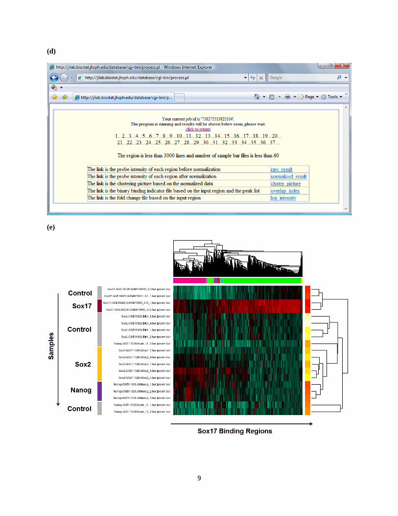
(v) If your input region file contains less than 3000 lines and the number of selected

samples is less than 60, a PDF file named "cluster*.pdf" will be returned. The file

contains a heat map showing the hierarchical clustering of the samples and genomic

regions based on the normalized intensities. The clustering uses average linkage, and 1-

Pearson's correlation as the distance measure.

Note: If the number of your input regions is more than 3000 lines or the number of

selected samples is more than 60, we will not return the PDF file with the heat map, since

3

the clustering may take significant amount of computational resource and may affect

other users/jobs. We recommend you to do your own clustering using dChip.

EXAMPLES

Example S1. A step-by-step illustration of the analysis of mouse Sox17, Oct4, Sox2 and Nanog data. The

Sox17 binding regions used in this analysis are obtained from Niakan et al. (2010) and can be

downloaded from the hmChIP website. They are stored in a COD file. A COD file is a tab-delimited text

file with at least five columns. The first five columns are region identifier, chromosome, region start,

region end, and region strand information (the strand is not used in hmChIP analysis). Below is a sample

line in the file:

geneA chr1 2000 2300 +

One can perform the hmChIP analysis as follows.

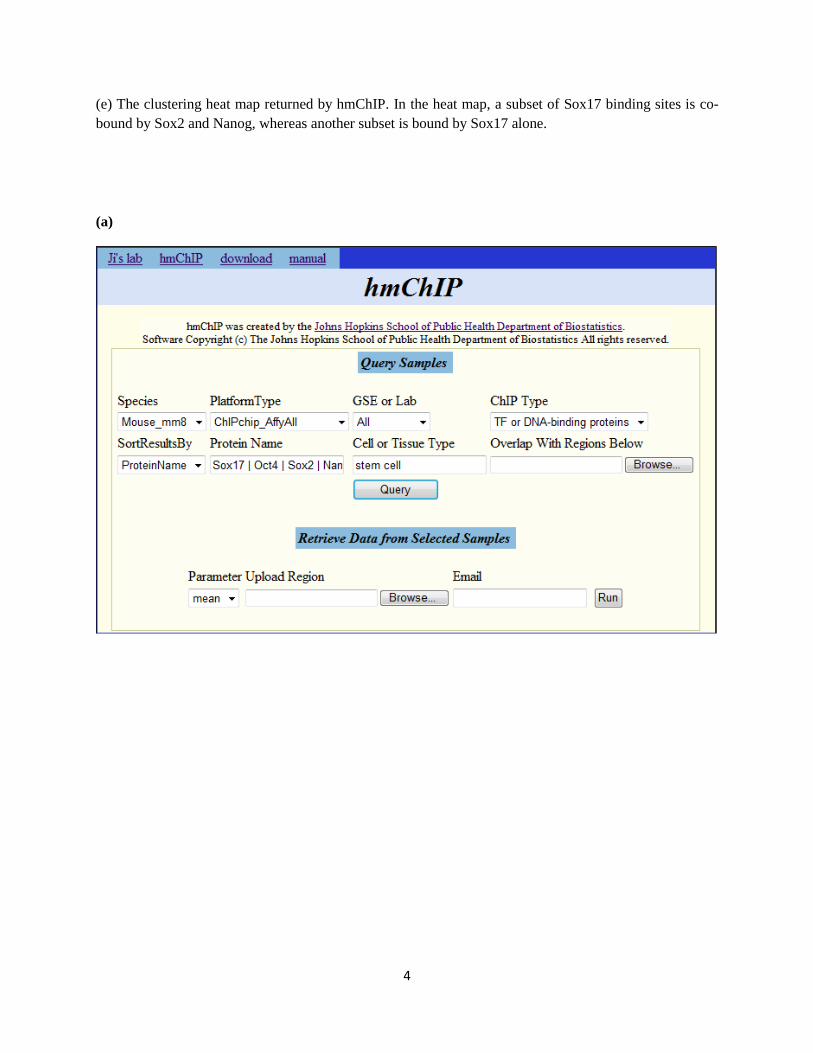
(a) Query mouse ChIP-chip samples. Choose species = mouse_mm8, platform type = ChIPchip_AffyAll,

GSE or lab = All, ChIP Type = TF or DNA-binding proteins, protein name = Sox17 | Oct4 | Sox2 |

Nanog, cell or tissue type = stem cell, then click the “Query” button. Note that multiple proteins and cell

types can be queried together by using „|‟ (i.e. OR) to separate them.

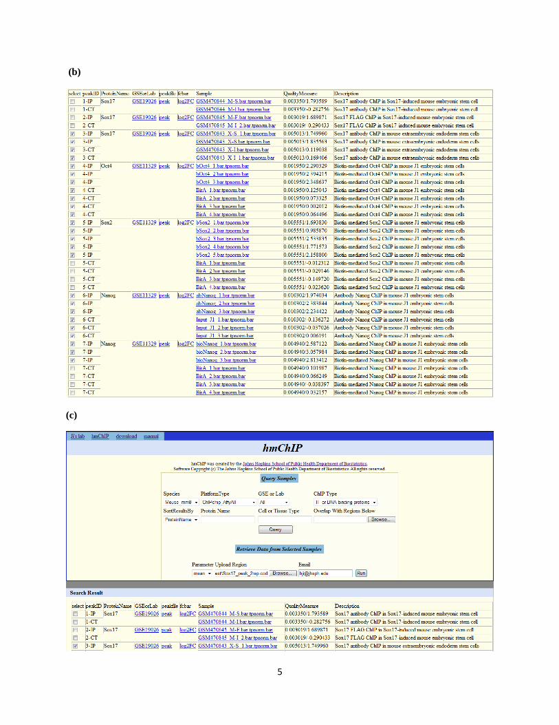
(b) In the query results, all mouse ChIP-chip experiments and samples matching the key words are listed.

Links to peak lists, log2 fold change profiles of experiments, and binding intensity profiles of samples are

provided to download these data. In the quality measure column, two numbers are provided. They are

percentage of genome covered by peaks, and log2 signal-to-noise ratio.

Select samples of interest from the query results. These include Sox17 IP and control samples in

extraembryonic endoderm (XEN) stem cells (i.e., samples labeled with X-S and X-I), all Oct4, Sox2 and

Nanog IP samples, and BirA and Input controls. Note that control samples labeled by “BirA” are shared

by several experiments. Only one copy needs to be selected. The Sox17 samples labeled with M-F, M-S

and M-I are not used in this analysis, since they are from mESC in which Sox17-DNA binding is weak.

(c) Go to the section titled “Retrieve Data from Selected Samples”. Provide genomic coordinates of

Sox17 binding sites in a COD file, and provide an email address. Click the “Run” button.

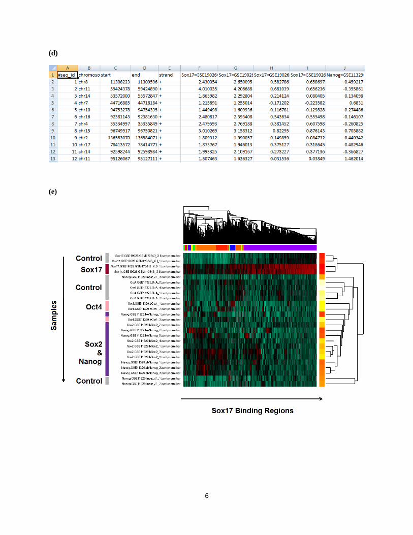
(d) The raw and normalized binding intensities (for each region and sample), binary binding indicators

(one number for each region and peak list), and log2 IP/control fold changes (one for each region and

peak list) will be returned by hmChIP through email. The data can be opened using Excel. Note that for

some of the Sox17 binding regions, the binary indicators are zero even for the Sox17 peak list. This is

because the Sox17 binding regions used in this analysis were obtained from Niakan et al. (2010), and they

are slightly different from the Sox17 peak list in hmChIP which was generated using a different analysis

procedure.

4

(e) The clustering heat map returned by hmChIP. In the heat map, a subset of Sox17 binding sites is co-

bound by Sox2 and Nanog, whereas another subset is bound by Sox17 alone.

(a)

5

(b)

(c)

6

(d)

(e)

7

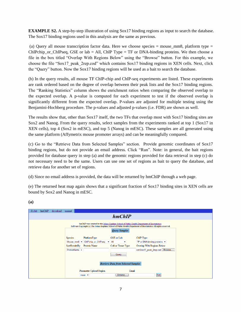
EXAMPLE S2. A step-by-step illustration of using Sox17 binding regions as input to search the database.

The Sox17 binding regions used in this analysis are the same as previous.

(a) Query all mouse transcription factor data. Here we choose species = mouse_mm8, platform type =

ChIPchip_or_ChIPseq, GSE or lab = All, ChIP Type = TF or DNA-binding proteins. We then choose a

file in the box titled “Overlap With Regions Below” using the “Browse” button. For this example, we

choose the file “Sox17_peak_2rep.cod” which contains Sox17 binding regions in XEN cells. Next, click

the “Query” button. Now the Sox17 binding regions will be used as a bait to search the database.

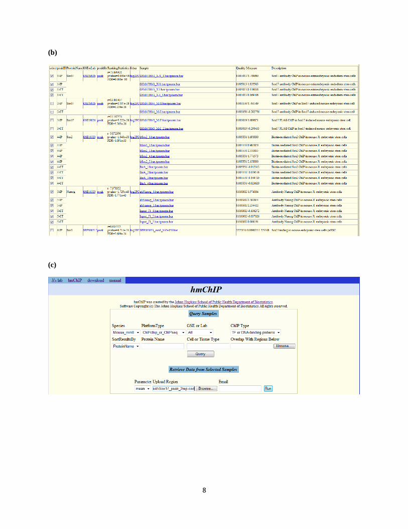
(b) In the query results, all mouse TF ChIP-chip and ChIP-seq experiments are listed. These experiments

are rank ordered based on the degree of overlap between their peak lists and the Sox17 binding regions.

The “Ranking Statistics” column shows the enrichment ratios when comparing the observed overlap to

the expected overlap. A p-value is computed for each experiment to test if the observed overlap is

significantly different from the expected overlap. P-values are adjusted for multiple testing using the

Benjamini-Hochberg procedure. The p-values and adjusted p-values (i.e. FDR) are shown as well.

The results show that, other than Sox17 itself, the two TFs that overlap most with Sox17 binding sites are

Sox2 and Nanog. From the query results, select samples from the experiments ranked at top 1 (Sox17 in

XEN cells), top 4 (Sox2 in mESC), and top 5 (Nanog in mESC). These samples are all generated using

the same platform (Affymetrix mouse promoter arrays) and can be meaningfully compared.

(c) Go to the “Retrieve Data from Selected Samples” section. Provide genomic coordinates of Sox17

binding regions, but do not provide an email address. Click “Run”. Note: in general, the bait regions

provided for database query in step (a) and the genomic regions provided for data retrieval in step (c) do

not necessary need to be the same. Users can use one set of regions as bait to query the database, and

retrieve data for another set of regions.

(d) Since no email address is provided, the data will be returned by hmChIP through a web page.

(e) The returned heat map again shows that a significant fraction of Sox17 binding sites in XEN cells are

bound by Sox2 and Nanog in mESC.

(a)

8

(b)

(c)

9

(d)

(e)

10

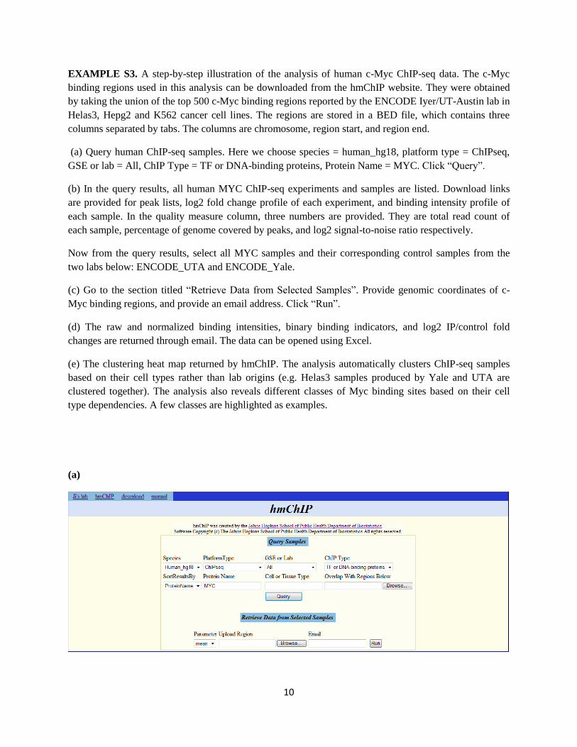
EXAMPLE S3. A step-by-step illustration of the analysis of human c-Myc ChIP-seq data. The c-Myc

binding regions used in this analysis can be downloaded from the hmChIP website. They were obtained

by taking the union of the top 500 c-Myc binding regions reported by the ENCODE Iyer/UT-Austin lab in

Helas3, Hepg2 and K562 cancer cell lines. The regions are stored in a BED file, which contains three

columns separated by tabs. The columns are chromosome, region start, and region end.

(a) Query human ChIP-seq samples. Here we choose species = human_hg18, platform type = ChIPseq,

GSE or lab = All, ChIP Type = TF or DNA-binding proteins, Protein Name = MYC. Click “Query”.

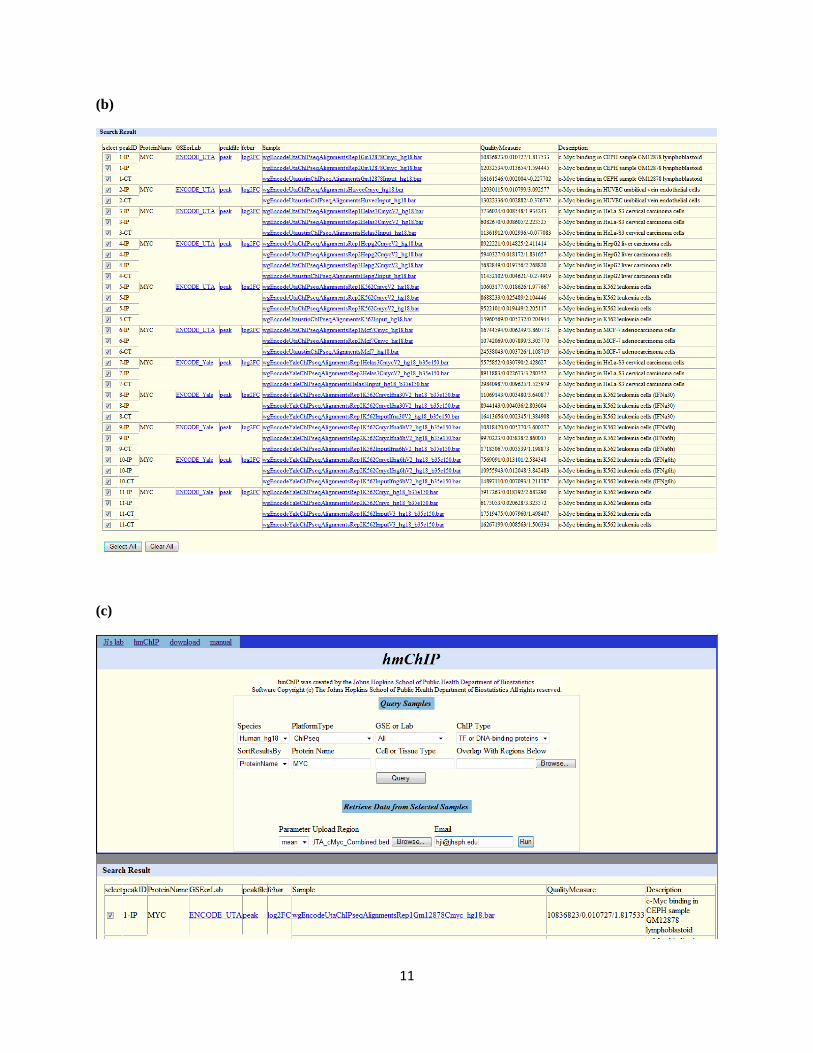
(b) In the query results, all human MYC ChIP-seq experiments and samples are listed. Download links

are provided for peak lists, log2 fold change profile of each experiment, and binding intensity profile of

each sample. In the quality measure column, three numbers are provided. They are total read count of

each sample, percentage of genome covered by peaks, and log2 signal-to-noise ratio respectively.

Now from the query results, select all MYC samples and their corresponding control samples from the

two labs below: ENCODE_UTA and ENCODE_Yale.

(c) Go to the section titled “Retrieve Data from Selected Samples”. Provide genomic coordinates of c-

Myc binding regions, and provide an email address. Click “Run”.

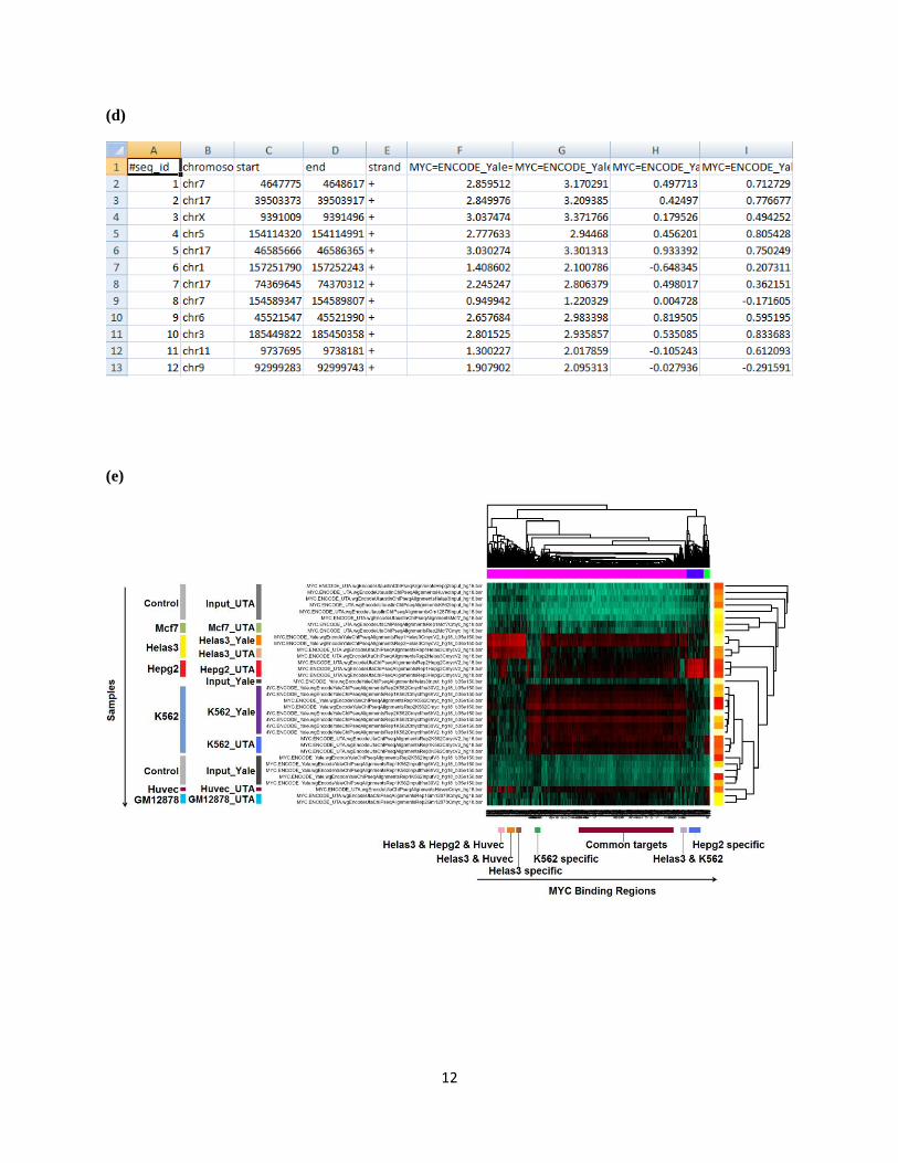
(d) The raw and normalized binding intensities, binary binding indicators, and log2 IP/control fold

changes are returned through email. The data can be opened using Excel.

(e) The clustering heat map returned by hmChIP. The analysis automatically clusters ChIP-seq samples

based on their cell types rather than lab origins (e.g. Helas3 samples produced by Yale and UTA are

clustered together). The analysis also reveals different classes of Myc binding sites based on their cell

type dependencies. A few classes are highlighted as examples.

(a)

11

(b)

(c)

12

(d)

(e)