HLMdiag: A Suite of Diagnostics for Hierarchical Linear ... · 2 HLMdiag: A Suite of Diagnostics...
28
JSS Journal of Statistical Software January 2014, Volume 56, Issue 5. http://www.jstatsoft.org/ HLMdiag: A Suite of Diagnostics for Hierarchical Linear Models in R Adam Loy Lawrence University Heike Hofmann Iowa State University Abstract Over the last twenty years there have been numerous developments in diagnostic pro- cedures for hierarchical linear models; however, these procedures are not widely imple- mented in statistical software packages, and those packages that do contain a complete framework for model assessment are not open source. The lack of availability of diag- nostic procedures for hierarchical linear models has limited their adoption in statistical practice. The R package HLMdiag provides diagnostic tools targeting all aspects and levels of continuous response hierarchical linear models with strictly nested dependence structures fit using the lmer() function in the lme4 package. In this paper we discuss the tools implemented in HLMdiag for both residual and influence analysis. Keywords : hierarchical linear models, diagnostics, residuals, influential observations, R. 1. Introduction Nested data structures—observations organized in non-overlapping groups—arise naturally from numerous data collection schemes. These structures occur when individuals are observed over time (longitudinal repeated measures data); when a field is subdivided into smaller plots on which a treatment is applied (split plots); or when a stratified sampling scheme is used, such as when sampling students within schools within districts (multilevel data). When data are organized in this manner it is clear that the observations are no longer independent, so any statistical model used must allow for a more general dependence structure where observations belonging to the same group can be correlated. Hierarchical linear models (HLMs)—also referred to as mutlilevel models, mixed effects models, random coefficients models, and ran- dom effects models—allow for such a dependence structure. HLMs incorporate parameters associated with the global trend—the fixed effects—and parameters associated with the in- dividual observations—the random effects—that govern the variance-covariance structure of
Transcript of HLMdiag: A Suite of Diagnostics for Hierarchical Linear ... · 2 HLMdiag: A Suite of Diagnostics...

JSS Journal of Statistical SoftwareJanuary 2014, Volume 56, Issue 5. http://www.jstatsoft.org/
HLMdiag: A Suite of Diagnostics for Hierarchical
Linear Models in R
Adam LoyLawrence University
Heike HofmannIowa State University
Abstract
Over the last twenty years there have been numerous developments in diagnostic pro-cedures for hierarchical linear models; however, these procedures are not widely imple-mented in statistical software packages, and those packages that do contain a completeframework for model assessment are not open source. The lack of availability of diag-nostic procedures for hierarchical linear models has limited their adoption in statisticalpractice. The R package HLMdiag provides diagnostic tools targeting all aspects andlevels of continuous response hierarchical linear models with strictly nested dependencestructures fit using the lmer() function in the lme4 package. In this paper we discuss thetools implemented in HLMdiag for both residual and influence analysis.
Keywords: hierarchical linear models, diagnostics, residuals, influential observations, R.
1. Introduction
Nested data structures—observations organized in non-overlapping groups—arise naturallyfrom numerous data collection schemes. These structures occur when individuals are observedover time (longitudinal repeated measures data); when a field is subdivided into smaller plotson which a treatment is applied (split plots); or when a stratified sampling scheme is used,such as when sampling students within schools within districts (multilevel data). When dataare organized in this manner it is clear that the observations are no longer independent, so anystatistical model used must allow for a more general dependence structure where observationsbelonging to the same group can be correlated. Hierarchical linear models (HLMs)—alsoreferred to as mutlilevel models, mixed effects models, random coefficients models, and ran-dom effects models—allow for such a dependence structure. HLMs incorporate parametersassociated with the global trend—the fixed effects—and parameters associated with the in-dividual observations—the random effects—that govern the variance-covariance structure of

2 HLMdiag: A Suite of Diagnostics for Hierarchical Linear Models in R
Residual HLM MLwiN SuperMix PROC MIXED xtmixed gllamm nlme lme4 HLMdiag
Marginal X XLevel-1 X∗ X X X X X X X X∗c
Higher-level X∗ X X X X X X X X∗c
Deletion X X X
Table 1: Overview of readily available residuals for commonly used statistical software. Notethat HLM and HLMdiag can calculate both least squares and empirical Bayes residuals (wedenote this by ∗ in the above table). Also, HLMdiag cannot calculate least squares residualsfor cross-classified models, but can calculate empirical Bayes residuals (we denote this by cin the above table).
the model. Compared to the linear model, additional complexities are introduced in theprocess of both model fitting and model checking due to the dependence structure and theincorporation of explanatory variables from each level of the data hierarchy. For example, inthe analysis of exam scores, observations may have been collected on both the student (theindividual or level-1 unit) and the school level (the group or level-2 unit).
For the linear model fit by ordinary least squares, residual analysis and influence analysis arewell-established staples both in practice and in the literature (Belsley, Kuh, and Welsch 1980;Cook and Weisberg 1982). In the last twenty years there have been numerous developments indiagnostic procedures for HLMs, which have primarily focused on the formulation of deletiondiagnostics (e.g., Cook’s distance), leverage, and outlier detection at each level of these models.We refer the reader to Loy and Hofmann (2013) for a recent review of available diagnosticsfor HLMs. While these developments greatly improve an analyst’s ability to check a fittedmodel, the incorporation of diagnostics into statistical software has lagged behind.
As noted by West and Galecki (2011), there are many software programs and packages capableof fitting HLMs: some are specialized programs dedicated only to this class of model whileothers are add-ons to general statistical software packages. Examples of specialized programsinclude HLM, MLwiN, and SuperMix (Raudenbush, Bryk, Cheong, Condon, and du Toit2011; Rasbash, Steele, Browne, and Goldstein 2012; Hedeker, Gibbons, Toit, and Patterson2008), and examples of package add-ons include PROC MIXED in SAS (SAS Institute Inc. 2008),xtmixed and gllamm in Stata (StataCorp 2007; Rabe-Hesketh, Skrondal, and Pickles 2004),and nlme and lme4 in R (Pinheiro, Bates, DebRoy, Sarkar, and R Core Team 2013; Bates,Maechler, and Bolker 2013a; R Core Team 2013). Residual analysis is well developed forall of the above programs and packages (Table 1), however, influence analysis is strikinglyunderdeveloped (Table 2). Currently, SAS is the only program to provide some tools todiagnose each aspect of the model.
In R, there are packages that work toward an exhaustive diagnosis of a fitted model, butnone are complete. The LMERConvenienceFunctions package (Tremblay and Ransijn 2013)provides model criticism plots based on the level-1 residuals through the function mcp.fnc,and the influence.ME package (Nieuwenhuis, Pelzer, and te Grotenhuis 2013; Nieuwenhuis,te Grotenhuis, and Pelzer 2012) provides access to influence measures for the fixed effectsparameters for models fit using the lme4 package. As seen in Tables 1 and 2, HLMdiagfills the need for accessible diagnostics for HLMs in R, implementing a unified and completeframework to access influence diagnostics and residuals. The package requires that modelshave strictly nested dependence structure (for full functionality) and are fit using lmer() in

Journal of Statistical Software 3
PROC
Diagnostic HLM MLwiN SuperMix MIXED xtmixed gllamm nlme lme4 HLMdiag
ParameterestimatesCook’s D FE, VC FE∗ FEc
MDFFITS FE, VC FEc
DFBETAS FE∗, VC∗
RVC VCc
Precision ofestimatesCOVTRACE FE, VC FEc
COVRATIO FE, VC FEc
Fitted valuesLeverage X X XPRESS XDFFITS X
Table 2: Overview of readily available tools for influence analysis for commonly used statisticalsoftware. FE denotes diagnostics for the fixed effects and VC denotes diagnostics for thevariance components. Note that a ‘∗’ indicates that the specified diagnostics are availablefor higher-level units in gllamm, and a ‘c’ indicates that the specified diagnostics are alsoavailable for cross-classified models in HLMdiag.
the package lme4.
Next, we introduce the notation for HLMs and the data example that is used throughout thepaper.
1.1. Hierarchical linear models
The discussion throughout this paper focuses on two-level HLMs for ease of explanation,however, it should be noted that the tools provided by HLMdiag can be used with higher-level models. The two-level HLM can be formulated through two equations specifying thewithin-group (level-1) and between-group (level-2) models
yi = Ziβi + εi (1)
βi = Wiγ + bi. (2)
In the above equations i = 1, . . . ,m denotes the group, yi is an ni × 1 vector of outcomes,Zi is an ni × q design matrix of level-1 explanatory variables, βi is a q × 1 vector of un-known fixed parameters, Wi is a q × p design matrix of level-2 explanatory variables, γ isa p × 1 vector of fixed effects, and bi is a q × 1 vector of random effects. Additionally, wewill assume that errors are independent normal between groups and different levels, that is,εi ∼ N(0, σ2Ii), bi ∼ N(0, σ2 D), and that COV(εi,bi) = 0. These assumptions imply thatyi ∼ N(ZiWiγ, σ
2Vi) where Vi = Ii + ZiDZ>i . Combining the within- and between-groupmodels we obtain a form of the linear mixed model (cf., e.g., Pinheiro and Bates 2000):
yi = Xiβ + Zibi + εi (3)
where Xi = ZiWi and β = γ from the two-level formulation. The HLM is extended to morelevels by incorporating additional random effects associated with the higher-level units.
4 HLMdiag: A Suite of Diagnostics for Hierarchical Linear Models in R
For general references on HLMs we refer the reader to Kreft and de Leeuw (1998), Raudenbushand Bryk (2002), Goldstein (2011), Hox (2010), and Snijders and Bosker (2012) who presentthese models in a social science framework. A more general treatment of these models can befound in Pinheiro and Bates (2000), McCulloch and Searle (2001), and Demidenko (2004).
1.2. Exam data
For illustrative purposes we make use of data on exam scores of 4,059 students in 65 inner-London schools. This data set is distributed as part of the R package mlmRev (Bates, Maech-ler, and Bolker 2013b), which makes well known multilevel modeling data sets available inR, and is analyzed in detail by Goldstein, Rasbash, Yang, Woodhouse, Pan, Nuttall, andThomas (1993) and more recently by Leckie and Charlton (2013).
R> data("Exam", package = "mlmRev")
R> head(Exam)
school normexam schgend schavg vr intake standLRT sex type student
1 1 0.2613 mixed 0.1662 mid 50% bottom 25% 0.6191 F Mxd 143
2 1 0.1341 mixed 0.1662 mid 50% mid 50% 0.2058 F Mxd 145
3 1 -1.7239 mixed 0.1662 mid 50% top 25% -1.3646 M Mxd 142
4 1 0.9676 mixed 0.1662 mid 50% mid 50% 0.2058 F Mxd 141
5 1 0.5443 mixed 0.1662 mid 50% mid 50% 0.3711 F Mxd 138
6 1 1.7349 mixed 0.1662 mid 50% bottom 25% 2.1894 M Mxd 155
For each student, the data consist of their gender (sex) and two standardized exam scores—an intake score on the London Reading Test (LRT) at age 11 (standLRT) and a score onthe General Certificate of Secondary Education (GCSE) examination at age 16 (normexam).Additionally, the students’ LRT scores were used to segment students into three categories(bottom 25%, middle 50%, and top 25%) based on their verbal reasoning subscore (vr) andoverall score (intake). At the school level, the data contain the average intake score for theschool (schavg) and type based on school gender (schgend, coded as mixed, boys, or girls).
Throughout Sections 2 and 3 we explore the relationship between a student’s intake score andtheir achievement on the GCSE examination. In Section 2 we focus on the use of residualsfor model selection and validation, and in Section 3 we search for influential students andschools.
2. Residual analysis
The presence of multiple sources of variability in HLMs results in numerous quantities definingresiduals. For this paper we will follow the classification by Hilden-Minton (1995) and definethree types of residuals (for a more general discussion of the types of residuals for linearmodels we refer the reader to Haslett and Haslett 2007):
1. level-1 (conditional) residuals, εi = yi − Xiβ − Zibi
2. level-2 (random effects) residuals, Zibi or, more commonly, bi
3. marginal (composite) residuals, ζi = yi − Xiβ = Zibi + εi.
Journal of Statistical Software 5
Note that these residuals are by definition confounded as they are interrelated. This con-founding of the residuals can lead to complications in the diagnosis of model deficiencies,since a violation in one type of residual may manifest itself as an alleged violation in a dif-ferent residual, so an analyst must be cautious. To cope with these confounded residualsHilden-Minton (1995) recommends an upward residual analysis, as it is possible to examinelevel-1 residuals that are unconfounded by other residuals (details below) while this is impos-sible in a downward residual analysis. This is the approach that we will follow in this section,starting with a discussion of level-1 residuals, followed by a discussion of level-2 residuals.
2.1. Level-1 residuals
The definition of the level-1 residuals
εi = yi − Xiβ − Zibi
leads to different residuals depending on how β and bi are estimated:
1. Least squares (LS):
Fitting separate linear models to each group and using LS to estimate β and bi leadsus to a first set of residuals. The benefit of this estimation procedure is that residualsdepend only on the lowest level of the hierarchy (level 1); thus the LS residual is uncon-founded by other residuals (Hilden-Minton 1995). While LS residuals are unconfoundedby the level-2 residuals, it is important to remember that for small within-group samplesizes the LS residuals will be unreliable. In such cases empirical Bayes residuals shouldbe used.
The LS level-1 residuals are calculated by fitting separate LS regression models for eachgroup and obtaining the residuals. In HLMdiag, LS models are fit using lmList()
in lme4 if there are no categorical explanatory variables that take on constant valueswithin the grouping factor. When a categorical explanatory variable does take on aconstant value within the grouping factor, separate LS models can still be fit, where theintercept simply absorbs the coefficient of the constant explanatory variable. HLMdiagautomates this process with the function adjust_lmList().
2. Empirical Bayes (EB):
The EB (shrinkage) residuals are defined as the conditional modes of the bis giventhe data and the estimated parameter values (which can be found either by maximumlikelihood or restricted maximum likelihood). The EB residuals at each level are in-terrelated, which makes us prefer LS residuals over the EB residuals at level-1, unlesssmall within-group sample sizes prevent the use of LS residuals.
For higher levels of the models our preference will be reversed: once the assumptions atthe lower level are checked, and the issue of confounding is taken care of, we suggest theuse of EB residuals over LS residuals. This is discussed in more detail in Section 2.2.
For ‘merMod’ objects, resid() returns the raw residuals from the model, that is, yi− yi,where yi = Xiβ − Zibi are the predicted conditional mean responses. The estimate bi
calculated by lmer() is an EB estimate; thus, resid() is an object specific function toextract the EB residuals from an ‘merMod’ object.

6 HLMdiag: A Suite of Diagnostics for Hierarchical Linear Models in R
We will highlight some of the functionality in the HLMdiag package for model building andvalidation using the exam data previously introduced. We fit an initial two-level HLM using astudent’s standardized London Reading Test intake score (standLRT) to explain their GCSEexam score allowing for a random intercept for each school:
R> (fm1 <- lmer(normexam ~ standLRT + (1 | school), Exam, REML = FALSE))
Linear mixed model fit by maximum likelihood ['lmerMod']
Formula: normexam ~ standLRT + (1 | school)
Data: Exam
AIC BIC logLik deviance
9365.243 9390.478 -4678.622 9357.243
Random effects:
Groups Name Std.Dev.
school (Intercept) 0.3035
Residual 0.7522
Number of obs: 4059, groups: school, 65
Fixed Effects:
(Intercept) standLRT
0.002391 0.563371
This model suggests that students with higher standLRT scores at age 11 generally scoredhigher on the GCSE exam at age 16. But is this model appropriate? To assess the appropri-ateness of model fm1 we must examine the level-1 and -2 residuals. Below we demonstrateusing HLMresid() to calculate the LS level-1 residuals from the fitted model.
R> resid1_fm1 <- HLMresid(fm1, level = 1, type = "LS", standardize = TRUE)
R> head(resid1_fm1)
normexam standLRT school LS.resid fitted std.resid
1 0.2613 0.6191 1 -0.5611 0.8225 -0.6824
2 0.1341 0.2058 1 -0.3953 0.5293 -0.4801
3 -1.7239 -1.3646 1 -1.1393 -0.5846 -1.4045
4 0.9676 0.2058 1 0.4383 0.5293 0.5323
5 0.5443 0.3711 1 -0.1022 0.6466 -0.1242
6 1.7349 2.1894 1 -0.2015 1.9364 -0.2512
To do this we set level = 1 and type = "LS". The standardized level-1 residuals are givenby
ε∗i = ∆−1/2i εi (4)
where ∆i is a diagonal matrix with elements equal to the diagonal of VAR(εi). Specifyingstandardize = TRUE indicates that the standardized residuals should also be returned. Alter-natively, we can specify standardize = "semi", which requests that the semi-standardizedresiduals (explanation below) be returned. For LS level-1 residuals a data frame is returnedconsisting of the model frame, LS residuals, fitted values, and, if requested, standardizedresiduals.

Journal of Statistical Software 7
−3
−2
−1
0
1
2
−2 0 2standLRT
LS le
vel−
1 re
sidu
als
Figure 1: Plot of the level-1 LS residuals vs. standardized LRT score. The smoother indicatesa potential nonlinear trend.
A plot of the LS level-1 residuals against the fitted values (not shown) showed no signs ofmodel misspecification at level 1; however, a plot of the LS level-1 residuals against thestandardized LRT scores (Figure 1)
R> qplot(x = standLRT, y = LS.resid, data = resid1_fm1,
+ geom = c("point", "smooth")) + ylab("LS level-1 residuals")
suggests that standardized LRT scores may not be linearly related to GCSE exam scores.Likelihood ratio tests (not shown) confirm that quadratic and cubic terms for standLRT
contribute significantly in describing GCSE exam scores, so we incorporate these terms in theupdated model, fm2.
R> fm2 <- lmer(normexam ~ standLRT + I(standLRT^2) + I(standLRT^3) +
+ (1 | school), Exam, REML = FALSE)
To check for homoscedasticity of the level-1 residuals, one strategy is to plot residuals againstexplanatory variables or any other potentially meaningful order of the points. For each group,i, the LS level-1 residuals, εi, have VAR(εi) = σ2i (1 − hi) where hi is a vector containing thediagonal elements of the hat matrix, Hi = Xi(X
>i Xi)
−1Xi, from the LS model fit. In order totarget the assumption of homoscedastic level-1 residuals we make use of the semi-standardizedresiduals (Snijders and Berkhof 2008)
εi = σiε∗i = σi∆
−1/2εi ∼ N(0, σ2I) (5)
The semi-standardized level-1 residuals are calculated from model fm2 below:
8 HLMdiag: A Suite of Diagnostics for Hierarchical Linear Models in R
−3
−2
−1
0
1
2
0.0 2.5 5.0 7.5standLRT2
sem
i−st
anda
rdiz
ed r
esid
uals
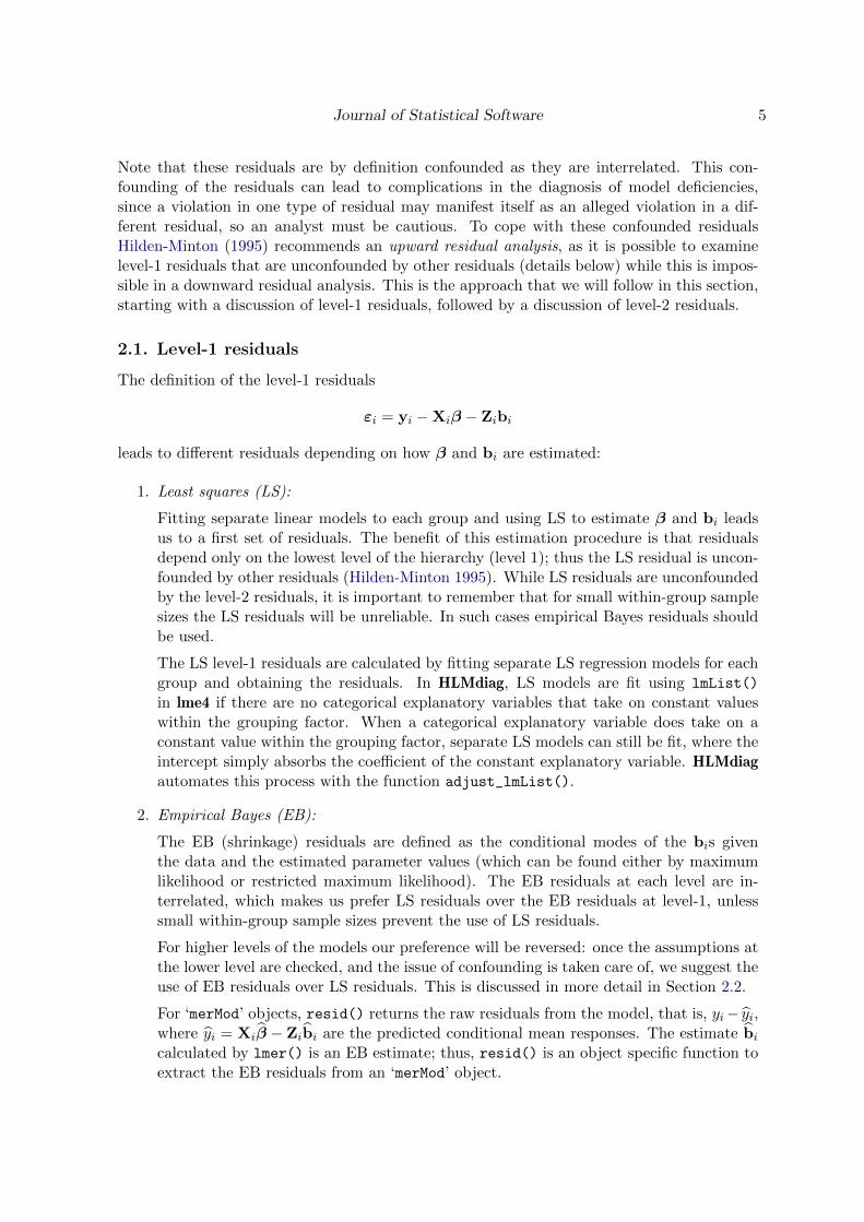
Figure 2: LS level-1 semi-standardized residuals against standLRT2 for the model includingthe quadratic and cubic terms. There is no indication of a violation of linearity; however, wenow see some evidence of heteroscedasticity.
R> resid1_fm2 <- HLMresid(fm2, level = 1, type = "LS", standardize = "semi")
R> head(resid1_fm2)
normexam standLRT I(standLRT^2) I(standLRT^3) school LS.resid
1 0.2613 0.6191 0.383234.... 0.237244.... 1 -0.65588
2 0.1341 0.2058 0.042354.... 0.008716.... 1 -0.39445
3 -1.7239 -1.3646 1.862067.... -2.54093.... 1 -1.06446
4 0.9676 0.2058 0.042354.... 0.008716.... 1 0.43907
5 0.5443 0.3711 0.137719.... 0.051108.... 1 -0.14143
6 1.7349 2.1894 4.793635.... 10.49536.... 1 -0.07961
fitted semi.std.resid
1 0.9172 -0.66523
2 0.5285 -0.39879
3 -0.6594 -1.09656
4 0.5285 0.44390
5 0.6858 -0.14311
6 1.8145 -0.08557
Figure 2 shows a plot of the semi-standardized residuals against standLRT2,
R> qplot(x = `I(standLRT^2)`, y = semi.std.resid, data = resid1_fm2) +
+ geom_smooth(method = "lm") + ylab("semi-standardized residuals") +
+ xlab("standLRT2")

Journal of Statistical Software 9
Figure 3: These twenty plots display the semi-standardized residuals from a hierarchical modelagainst one of the predictor variables. The plot of the real data is randomly embedded amongnineteen simulated plots. Which is the real plot?
and indicates a potential problem with heteroscedasticity. To further investigate this issue, weuse visual inference through the use of the lineup protocol proposed by Buja, Cook, Hofmann,Lawrence, Lee, Swayne, and Wickham (2009) (see Section A in the appendix for additionaldetails and code). Figure 3 displays this lineup. We find the plot of the original data tobe indistinguishable (refer to the appendix for the position of the data plot) from the plotsgenerated from the simulated data, indicating the perceived structure in the residual plot isan artifact of the sparsity of data for large values of standLRT; thus, we may proceed withthe analysis without the need for remedial measures.

10 HLMdiag: A Suite of Diagnostics for Hierarchical Linear Models in R
−3
−2
−1
0
1
2
−4 −2 0 2 4Theoretical Quantiles
Sam
ple
Qua
ntile
s
Figure 4: Normal quantile plot of the semi-standardized level-1 residuals, constructed withthe ggplot_qqnorm() function.
An alternative way to check homoscedasticity of level-1 residuals is to use boxplots of thelevel-1 residuals by group to assess within-group homoscedasticity. If the assumption ofwithin-group homoscedasticity is plausible, then the boxplots should exhibit roughly constantinterquartile ranges (IQRs). We omit this approach for brevity.
Figure 4 displays a normal quantile plot of the semi-standardized level-1 residuals
R> ssresid <- na.omit(resid1_fm2$semi.std.resid)
R> ggplot_qqnorm(x = ssresid, line = "rlm")
and shows that the semi-standardized residuals appear normal except for the very low valueswhere the values are larger in absolute value than expected; however, this discrepancy is quitesmall and does not offer much evidence against the assumption of normality.
In an exploratory setting we would go through this cycle of residual analysis, identificationof explanatory variables, and model fitting multiple times until a satisfactory level-1 model isfound (Tukey 1977). Since LS level-1 residuals come from LS fits, we can pair the evaluationof the goodness-of-fit of a model with the regular tools we have in this situation; such ascomparisons of nested models (through F tests or ANOVA) or stepwise regression diagnostics.
Carrying out this iterative process for the Exam data (not shown) results in the inclusion ofstudent gender in the model. Additionally, including a random slope for standardized LRT,allowing for the strength of relationship between the two exams to vary across schools, wasfound to significantly improve the model.
R> fm3 <- lmer(normexam ~ standLRT + I(standLRT^2) + I(standLRT^3) + sex +
+ (standLRT | school), Exam, REML = FALSE)

Journal of Statistical Software 11
2.2. Level-2 residuals
The level-2, or random effects, residuals are defined as Zibi or, more commonly, bi. Obviously,the method of estimation impacts on the value of this residual. Again, LS and EB are thetwo methods of estimation. We will discuss both briefly:
1. Least squares (LS):
Rearranging Equation 2, we see that this estimate is of the form bi = βi−Wiγ, whereβi is a vector of estimates from separate LS models and Wiγ is the estimated globaltrend. HLMresid() calculates these residuals using adjust_lmList() to fit the separateLS models whose coefficients are then compared to the global trend.
2. Empirical Bayes (EB):
bi is estimated using the conditional mode given the data and the estimated parametervalues. EB estimates of bi can be obtained directly from an ‘merMod’ object usingranef(), or by using HLMresid().
As stated above, if an upward residual analysis is followed, then we prefer the use ofEB residuals at level 2. Our preference stems from the fact that the LS residuals are farmore variable than the corresponding residuals, so exploratory plots of omitted variableswill exhibit weaker associations than the corresponding plots of EB residuals, and thatfor small sample sizes LS residuals are untrustworthy or unavailable.
The level-2 residuals are used to
� identify additional explanatory variables that contribute significantly to the model,
� check linearity of the level-2 explanatory variables, and
� investigate whether the level-2 residuals follow a normal distribution.
To obtain the level-2 EB residuals from model fm3, we use the following code:
R> resid2_fm3 <- HLMresid(object = fm3, level = "school")
R> head(resid2_fm3)
(Intercept) standLRT
1 0.40367 0.12715
2 0.40082 0.15930
3 0.49475 0.07796
4 0.05969 0.11968
5 0.25134 0.07107
6 0.44792 0.04821
where the level refers to the name of the grouping factor contained in the data set. Noticethat we did not need to specify type = "EB" as it is the default setting. This returns a dataframe with columns corresponding to the EB estimates of the random intercept and slope.
Boxplots of the EB residuals for the intercept grouped by school gender (schgend, the leftside of Figure 5) show schgend is useful in explaining some of the between-school variability

12 HLMdiag: A Suite of Diagnostics for Hierarchical Linear Models in R
−0.4
0.0
0.4
mixed girls boysschool gender
leve
l−2
resi
dual
(In
terc
ept)
−0.4
0.0
0.4
−0.8 −0.4 0.0 0.4average intake score
leve
l−2
resi
dual
(In
terc
ept)
Figure 5: Plots of the level-2 EB residuals for the intercept plotted against the omittedexplanatory variables schgend and schavg. We construct boxplots for schgend to appropri-ately display a categorical variable and a scatterplot with a smoother to display a continuousvariable. The boxplots for schgend are not all centered around zero, indicating that the vari-able contains information useful in describing the between-school variation in exam scores.Similarly, we observe a positive association in the scatterplot for schavg.
and should be incorporated into the model. Similarly, a scatterplot of the EB residuals forthe intercept against the average intake score (schavg, on the right side of Figure 5) exhibitspositive association, indicating that schavg should be incorporated into the model. Below,we add the two variables as fixed effects.
R> fm4 <- lmer(normexam ~ standLRT + I(standLRT^2) + I(standLRT^3) + sex +
+ schgend + schavg + (standLRT | school), data = Exam, REML = FALSE)
We will refer to this model throughout the remainder of the paper.
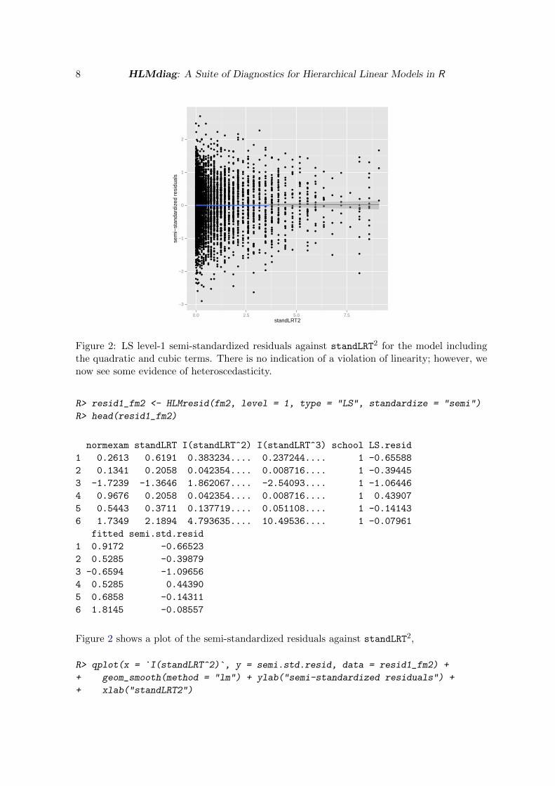
The assumption of normality of residuals is assessed by normal quantile plots for each of thelevel-2 residual vectors. Figure 6 shows normal quantile plots of the level-2 EB residuals forboth the intercept (left side) and slope (right side) terms, neither of which shows evidenceof a deviation from normality. One outlier is seen in the plot for the random slope and isdetermined to be school 53. An inspection of the records for this school did not yield anyimmediately apparent anomalies, but we will further investigate this school in the discussionon influential data points.
2.3. Marginal residuals
Marginal residuals are obtained by plugging in the estimate of β, β, into the definition
ζi = yi − Xiβ
Journal of Statistical Software 13
−0.6
−0.3
0.0
0.3
−2 −1 0 1 2Theoretical Quantiles
Sam
ple
Qua
ntile
s
−0.2
−0.1
0.0
0.1
0.2
0.3
−2 −1 0 1 2Theoretical Quantiles
Sam
ple
Qua
ntile
s
Figure 6: Normal quantile plots of the level-2 EB residuals for the intercept (left panel) andslope (right panel). The normal quantile plot for the random slope indicates that school 53is an outlier.
and are calculated from an ‘merMod’ object using HLMresid() specifying level = "marginal".These residuals can be used for diagnostics as they would be in single-level linear models; how-ever, as these residuals are the sum of the level-1 and level-2 residuals, any problems exhibitedmust be accompanied by analysis of the other types of residuals to pinpoint the source of theproblem. One situation in which the marginal residuals are uniquely valuable is in assessingthe marginal covariance structure, such as in repeated measures and longitudinal data, as themarginal residuals, ζi, and observed values, yi, have the same covariance structure.
2.4. Addressing residual deficiencies
In the above example, we did not observe significant model deficiencies, but if any had beenobserved remedial measures would have been necessary. In this section we briefly discuss suchmeasures available for the HLM.
To correct for nonlinearity, heteroscedasticity, or nonnormality, transformations of either theresponse variable or explanatory variables may prove helpful (Snijders and Bosker 2012, Chap-ter 10). For example, as in classical regression, an appropriate transformation of an explana-tory variable may correct for a nonlinear relationship with the response. Similarly, appropriatetransformations of the response variable can help correct heteroscedasticity and skewed resid-ual distributions. For examples of this we refer the reader to Gurka, Edwards, Muller, andKupper (2006) and Goldstein, Carpenter, Kenward, and Levin (2009), who discuss how touse the Box-Cox transformation to correct for nonnormal distributions.
While transformations present a rather straight forward approach to addressing model defi-ciencies it may be preferrable to reformulate the model with weaker distributional assump-tions. This approach has the advantage that the data will be represented in the originalscale of the problem, retaining greater interpretability. If heteroscedasticity in the residuals

14 HLMdiag: A Suite of Diagnostics for Hierarchical Linear Models in R
is discovered, the model assumptions can be weakened to allow the residual variance to de-pend upon some explanatory variable (Snijders and Bosker 2012, Chapter 8). Currently, itis not possible to model the residual variance as a function of covariates using lmer(); how-ever, this is possible using lme() in the R package nlme (we refer the reader to Pinheiro andBates 2000, Section 5.2 for details). If nonnormal residual distributions are discovered, thenthe distributional assumptions can be reformulated to more adequately represent the data,though model estimation may become more challenging. Alternatively, strong distributionalasssumptions on the random effects can be avoided through the use of semiparametric ornonparametric methods (Shen and Louis 1999; Zhang and Davidian 2001; Ghidey, Lesaffre,and Eilers 2004), or mixtures of normal distributions (Verbeke and Lesaffre 1996). We referthe reader to Ghidey, Lesaffre, and Verbeke (2010) for a recent review of these methods.
Although model reformulation leads to a more accurate representation of the data generatingmechanism, for analyses focused on estimation rather than prediction it may not be necessary.An alternative approach useful when normality is violated is the use of robust ‘sandwich’ esti-mators of the standard errors (Verbeke and Lesaffre 1997; Yuan and Bentler 2002), assumingsample sizes are large enough in the highest-level of the model.
3. Influence analysis
Influence analysis consists of systematically investigating whether some observation, or groupof observations, is given disproportionate importance in model estimation, and, consequently,on the conclusions made from the analysis. Such observations are deemed influential, and theanalyst must understand what impact these influential points have on the fitted model.
The most straightforward way to assess this influence is through the use of deletion diagnostics.Deletion diagnostics are statistics that quantify the change in a parameter estimate whensome subset of the data is deleted. These diagnostics are well documented in the literaturefor regression models (Belsley et al. 1980; Cook and Weisberg 1982) and are widely availablein statistical software; however, they are less established for HLMs (see Table 2).
Compared to the classical regression model, an additional complication is introduced by thehierarchical structure of the data for this class of models. Hierarchical data contain naturalclusters of observations, whereas the linear regression model assumes that observations areindependent, resulting in the need for multiple deletions to assess the influence of both indi-vidual observations and clusters of observations. Specifically, in the case of a two-level model,we refer to the deletion of an individual observation as a level-1 deletion and the deletionof an entire level-2 group as a level-2 deletion. Note that these definitions extend naturallyupward for models with additional levels in the hierarchy.
In this section we describe the implementation of diagnostics to assess changes in the estima-tion of the variance components using relative variance change, the estimation of the fixedeffects using Cook’s distance and a multivariate version of DFFITS (Belsley et al. 1980), theprecision of the fixed effects estimates using the covariance ratio and trace, and the fittedvalues using leverage. These quantities are used to assess the influence in both level-1 andlevel-2 units. First, we will consider deletion diagnostics for the fixed effects of a HLM, butnote that in an analysis we would begin with diagnostics for the variance components as thediagnostics for fixed effects require a specified covariance matrix. We reverse the order herefor ease of explanation.

Journal of Statistical Software 15
3.1. Diagnostics for fixed effects
Changes in parameter values
Two statistics that are commonly used for measuring changes in fixed effects are Cook’sdistance and MDFFITS, a multivariate version of the DFFITS statistic. Both statisticsmeasure the distance between the fixed effects estimates obtained from the full data and thoseobtained from the reduced data, and are generalized for the HLM as follows (see Christensen,Pearson, and Johnson 1992, and Schabenberger 2004):
Ci(β) =1
p
(β − β(i)
)>VAR(β)
−1 (β − β(i)
)(6)
MDFFITSi(β) =1
p
(β − β(i)
)> VAR(β(i))
−1 (β − β(i)
)(7)
where p is the rank of X and β(i) is the estimate of β when the ith unit is deleted. Notethat these definitions are general enough to allow for deletion at any level—for example, fora two-level model, in the case of level-1 deletion, i refers to an individual, whereas for level-2deletion i refers to a group.
The difference between the two statistics is that Cook’s distance scales the change in theparameter estimates by the estimated covariance matrix of the original parameter estimates,while MDFFITS is scaled by the estimated covariance matrix of the deletion estimates. Thismeans that computation of Cook’s distance only requires the covariance from the original fit-ted model while computation of MDFFITS requires the covariance structure to be reestimatedin the absence of the ith unit and the inverse to be recalculated.
Regardless of the statistic used, larger values indicate higher levels of influence. In the caseof unknown covariance structure we do not have an exact reference distribution for thesestatistics, so instead of relying on an approximation based on a large sample asymptoticresult, we adhere to the use of measures of relative standing to determine which units shouldbe considered for further investigation. For example, we might consider units associated withstatistics that are more than 1.5×IQR or 3×IQR above the third quartile (Q3) as extreme fordiagnostics where large values are indicative of a problem. In practice we have found the moreconservative cutoff, Q3+3×IQR, to be a more useful starting point for such an investigation,especially for large sample sizes, as it identifies “extreme” values of the empirical distributionof these diagnostics rather than all outlying values. An alternative strategy is to plot thestatistic and visually identify unusual values based on gaps in the empirical distribution.
HLMdiag implements both Cook’s distance and MDFFITS for ‘merMod’ objects. For ourexample we compute the level-2 (school-level) deletion statistics of model fm4 using the belowcode.
R> cooksd_fm4 <- cooks.distance(fm4, group = "school")
R> mdffits_fm4 <- mdffits(fm4, group = "school")
Both functions return a vector of diagnostic values and a list of the differences between theoriginal and deleted fixed effects parameter vectors (beta_cdd), β − β(i), as an attribute.
To evaluate diagnostic values, we use dotplots—or a modified version of them. The dotplot ismodified by grouping all“non-influential”units—as identified by the values of the diagnostic—into one group and displaying the influential groups as single cases. For the modified version
16 HLMdiag: A Suite of Diagnostics for Hierarchical Linear Models in R
●
●
●
●
●
●
●
●
●
●●
●
●
●
●
●
●
●
●
●
●
●
●
●
●
●
●
●
●
●
●
●
●
●
●
●
●
●
●
●
●
●●
●
●
●
●
●
●
●
●●
●
●
●
●
●
●
●●
●
●
●
●
25
485745385835172112
9373341496213396160343147
8205619
5221011641442154443
25023
43229185126
62736
152535528634665595430
37
24164025
0.000 0.025 0.050 0.075Cook's distance
scho
ol
●● ●●● ● ●●● ●●●● ● ● ●● ●●●● ● ● ●● ● ●● ●● ●● ●● ●●● ● ●● ● ●●● ●●● ● ● ● ● ● ●●●● ● ●●●● ●● ●
25
within cutoff
25
0.000 0.025 0.050 0.075Cook's distance
scho
ol
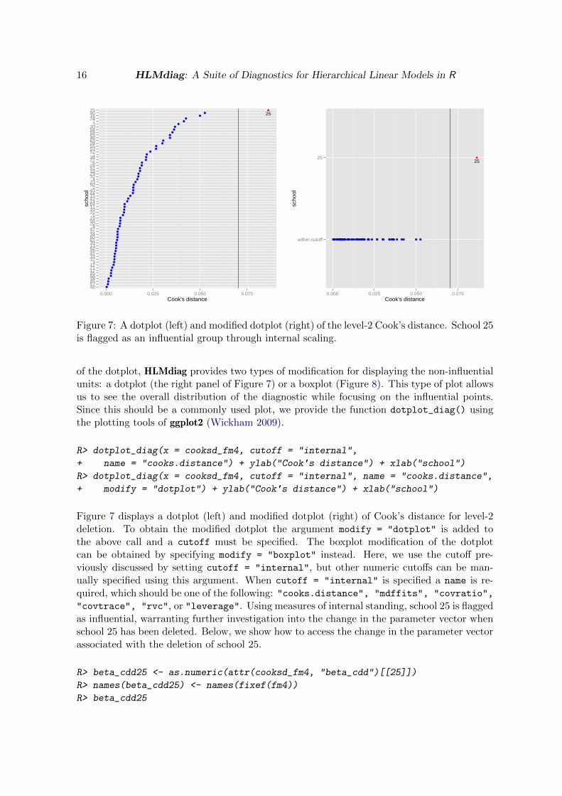
Figure 7: A dotplot (left) and modified dotplot (right) of the level-2 Cook’s distance. School 25is flagged as an influential group through internal scaling.
of the dotplot, HLMdiag provides two types of modification for displaying the non-influentialunits: a dotplot (the right panel of Figure 7) or a boxplot (Figure 8). This type of plot allowsus to see the overall distribution of the diagnostic while focusing on the influential points.Since this should be a commonly used plot, we provide the function dotplot_diag() usingthe plotting tools of ggplot2 (Wickham 2009).
R> dotplot_diag(x = cooksd_fm4, cutoff = "internal",
+ name = "cooks.distance") + ylab("Cook's distance") + xlab("school")
R> dotplot_diag(x = cooksd_fm4, cutoff = "internal", name = "cooks.distance",
+ modify = "dotplot") + ylab("Cook's distance") + xlab("school")
Figure 7 displays a dotplot (left) and modified dotplot (right) of Cook’s distance for level-2deletion. To obtain the modified dotplot the argument modify = "dotplot" is added tothe above call and a cutoff must be specified. The boxplot modification of the dotplotcan be obtained by specifying modify = "boxplot" instead. Here, we use the cutoff pre-viously discussed by setting cutoff = "internal", but other numeric cutoffs can be man-ually specified using this argument. When cutoff = "internal" is specified a name is re-quired, which should be one of the following: "cooks.distance", "mdffits", "covratio",
"covtrace", "rvc", or "leverage". Using measures of internal standing, school 25 is flaggedas influential, warranting further investigation into the change in the parameter vector whenschool 25 has been deleted. Below, we show how to access the change in the parameter vectorassociated with the deletion of school 25.
R> beta_cdd25 <- as.numeric(attr(cooksd_fm4, "beta_cdd")[[25]])
R> names(beta_cdd25) <- names(fixef(fm4))
R> beta_cdd25
Journal of Statistical Software 17
(Intercept) standLRT I(standLRT^2) I(standLRT^3) sexM
0.0038952 -0.0098668 -0.0033337 0.0032080 0.0009799
schgendboys schgendgirls schavg
0.0023156 -0.0167646 0.0220914
To obtain these diagnostics for level-1 units using cooks.distance() and mdffits() we setgroup = NULL.
Precision of fixed parameters
The covariance matrix of β gives insight into the precision of the parameter estimates. Boththe covariance trace (COVTRACE, Christensen et al. 1992) and the covariance ratio (COV-RATIO) are measures of how precision is effected by the deletion of unit i. Again, we makeuse of a general definition that allows us to examine level-specific dependencies at a laterpoint:
COVTRACEi(β) =
∣∣∣∣trace
(VAR(β)
−1· VAR(β(i))
)− p
∣∣∣∣ (8)
COVRATIOi(β) = det
(
VAR(β(i))
)(det
(VAR(β)
))−1(9)
Both statistics compare the covariance matrices of β where β is estimated with and withoutunit i. Taking the covariance matrix of β with unit i as the baseline, COVTRACE comparesthe ratio of the two matrices to the p×p identity matrix, which has a trace of p. COVRATIOdirectly compares the volume of the matrices via their determinants. In the case that unit i isnot influential, the covariance trace will be close to zero, while the covariance ratio is close toone. As with Cook’s distance and MDFFITS, we recommend the use of measures of relativestanding or the visual identification of gaps in the empirical distribution to evaluate how farthe statistics must deviate from zero or one to be considered influential.
We calculate COVTRACE and COVRATIO for model fm4 by
R> covratio_fm4 <- covratio(fm4, group = "school")
R> covtrace_fm4 <- covtrace(fm4, group = "school")
An investigation of the results reveals that no schools are influential with respect to theprecision of the fixed effects estimates.
3.2. Diagnostics for variance components
Let θ denote the vector of variance components, that is, the vector containing the residualvariance, σ2, and the unique entries of D. The deletion diagnostics presented for fixed effectscan be adapted to the variance components by substituting θ and θ(i) in place of β and
β(i). Equations 10 through 13 display the analogs of the previously discussed diagnostics forvariance components.

18 HLMdiag: A Suite of Diagnostics for Hierarchical Linear Models in R
Di(θ) =(θ − θ(i)
)> VAR(θ)−1
(θ − θ(i)
)(10)
MDFFITSi(θ) =(θ − θ(i)
)> VAR(θ(i))−1
(θ − θ(i)
)(11)
COVTRACEi(θ) =
∣∣∣∣trace
(VAR(θ)
−1· VAR(θ(i))
)− q
∣∣∣∣ (12)
COVRATIOi(θ) = det
(
VAR(θ(i))
)(det
(VAR(θ)
))−1(13)
Note that the formulas for Cook’s distance and MDFFITS (Equations 10 and 11) no longercontain division by the rank of X, and in Equation 12 q denotes the rank of the covariancematrix of VAR(θ) (see Christensen et al. 1992 and Schabenberger 2004 for a discussion).Computationally, these diagnostics are more challenging as they are based on an estimateof the covariance matrix—such as the inverse Hessian matrix—for the variance components,which is not readily available for ‘merMod’ objects. While it would be possible to get anestimate of the covariance matrix for variance components using a parametric bootstrap, thiswould significantly increase the computational complexity. Instead, we focus on diagnosticsthat do not require an estimate of the covariance matrix, allowing the direct use of outputfrom lmer().
One diagnostic measure that meets this requirement is the relative variance change (RVC)(Dillane 2005), which measures the change in estimates of the `th variance component, θ`,with and without unit i. RVC is defined as
RVCi(θ`) =θ`(i)
θ`− 1, (14)
where θ`(i) is the estimate of the variance component when the ith unit is deleted, and θ` isthe estimate of the variance component obtained for the full data. RVC is close to zero whenunit i does not have a large influence on the variance component.
For model fm4, RVC is calculated for each school as
R> rvc_fm4 <- rvc(fm4, group = "school")
R> head(rvc_fm4)
sigma2 D11 D21 D22
1 -0.0029219 0.03895 -0.052570 0.038681
2 -0.0086459 0.08409 -0.037762 0.002719
3 -0.0025709 0.04303 0.058292 0.061995
4 -0.0001542 0.09395 0.004224 0.004319
5 0.0024723 0.07668 0.014645 0.039970
6 0.0026265 0.08395 0.065138 0.058902
The command rvc returns a matrix with named columns for each variance component, wheresigma2 is the residual variance, σ2, and D** denotes the unique entries of D where the trailingdigits denote the position in the matrix. In this example, D11 is the variance associated with

Journal of Statistical Software 19
7
5353
7
within cutoff
−0.3 −0.2 −0.1 0.0 0.1RVC
scho
ol
Figure 8: Modified dotplot of the level-2 RVC for the slope, that is, standLRT. Schools 7 and53 are flagged as influential by internal scaling.
the random intercept for schools, D22 is the variance associated with the random slope forstandardized LRT score, and D21 is the covariance associated with the random slope andrandom intercept.
Figure 8 displays a modified dotplot of the level-2 RVC for the random slope, standLRT.Through the use of internal scaling, schools 7 and 53 are identified as influential and warrantfurther investigation: school 53 appears to be a school with very good students (top verbalreasoning intake scores and above median exam and standLRT scores), and school 7 appearsto “pull students up” (mediocre verbal reasoning intake scores and median standLRT belowoverall median but exam scores higher than the overall median).
3.3. Diagnostics for fitted values
In addition to exploring how subsets of observations directly impact the model parameters,it is also of interest to explore whether these observations are unusual with regard to thefitted values and explanatory variables. This is done by exploring the leverage of subsetsof interest. As with linear regression, leverage can be defined as the rate of change in thepredicted response with respect to the observed response (Demidenko and Stukel 2005; Nobreand Singer 2011). Formally, assuming that VAR(yi) = σ2Vi is fixed, the leverage at level ican be defined as
Hi =∂y∗i∂yi
= Xi
(X>i V−1i Xi
)−1X>i V−1i + ZiDZ>i V−1i (I − H1i) (15)
= H1i + H2i
20 HLMdiag: A Suite of Diagnostics for Hierarchical Linear Models in R
where y∗i = Xiβ + Zibi. In the above definition, leverage is described in two parts, whichwe refer to as the leverage associated with the fixed effects, H1i, and the leverage associatedwith the random effects, H2i. The leverage associated with the random effects depends onthe leverage associated with the fixed effects; thus, using H2i we are unable to separate thetwo components. Alternatively, the random effects leverage can be defined as
H∗2i = ZiDZ>i (16)
which is unconfounded by the fixed effects (Nobre and Singer 2011).
Using Equations 15 and 16, we define the leverage of observation j in group i to be equal tothe jth diagonal element of the leverage matrix of interest, and the leverage of group i to bethe mean of the diagonal elements of the leverage matrix of interest. To reflect the plurality ofstatistics that can be defined as “leverage” in a hierarchical model, leverage() in HLMdiagreturns numerous quantities: the overall leverage (overall, H), the fixed effects leverage(fixef, H1), the random effects leverage (ranef, H2), and the unconfounded random effectsleverage (ranef.uc, H∗2).
R> leverage_fm4 <- leverage(fm4, level = "school")
R> head(leverage_fm4)
overall fixef ranef ranef.uc
1 0.02171 0.001869 0.01984 0.1568
2 0.02667 0.002372 0.02430 0.1758
3 0.02573 0.002564 0.02316 0.1725
4 0.02011 0.001629 0.01848 0.1497
5 0.03134 0.001890 0.02945 0.1437
6 0.01790 0.001913 0.01599 0.1814
From an investigation of the resulting leverage for the fixed effects (fixef) we find that schools37, 48, and 54 have high leverage. Interestingly, no schools are flagged as having high leverageon the random effects when using the unconfounded version (ranef.uc), while schools 48 and54 are flagged when using the confounded version (ranef)—this supports our preference forinvestigation of the unconfounded version of leverage. With a more thorough investigationof the schools, we determine the schools are not influential. The flagged schools are nearthe extremes of the average intake scores, explaining why they were flagged, but none of theschools deviate much from the overall trend.
3.4. Addressing influential and outlying units
Having identified potential influential and outlying units, we consider modeling approachesto appropriately represent these units. First, when an influential or outlying unit is identifiedit is important to carefully explore the values of the response and explanatory variables fordata entry errors and other peculiarities. If the identified units appear to be different withrespect to some observed explanatory variable one approach is to include a dummy variablein the model explaining the apparent difference (for an example of this approach we referthe reader to Langford and Lewis 1998). This can also be used to adjust the intercept whenno such explanatory variable is found. Occassionally, a unit may be detected that is from a

Journal of Statistical Software 21
population other than that of interest, in which case deletion of this unit from the data set isa viable option.
An alternative approach to address the issue of outlying and influential units is the useof robust methods protecting against the influence of such units. The use of heavy-taileddistributions for the residuals, such as the t distribution, to protect against the impactsof outlying units have been proposed by Pinheiro, Liu, and Wu (2001) and Staudenmayer,Lake, and Wand (2009). Additionally, Demidenko (2004, Section 4.4) discusses alternativeapproaches to robust modeling.
4. Package description
In this section we provide additional description of the functions provided by HLMdiag.Tables 3 and 4 outline the main functions for residual and influence analysis included in thepackage accompanied by brief descriptions.
For residual analysis, HLMresid() provides a unified framework to calculate either LS orEB residuals at any level of the model. While EB residuals were previously available from‘merMod’ objects using resid() and ranef(), LS residuals required manual implementation bythe user. Additionally, HLMresid() provides the necessary framework to conduct an upwardresidual analysis without the need for programming on the part of the user.
HLMdiag also provides the most complete suite of tools for influence analysis available in R,comparable to those available in SAS PROC MIXED. Among the functions outlined in Table 4it is important to note that HLMdiag provides two implementations of cooks.distance,mdffits, covratio, and covtrace: one based on the full model refit, and the other basedon a one-step approximation. The example discussed in the above sections illustrated the“fast” implementation based on one-step approximations for the fixed effects and associatedcovariance matrices (for further details we refer the reader to Christensen et al. 1992; Shiand Chen 2008; Zewotir 2008). The implementation of these approximations utilizes smaller,dense submatrices resulting in more efficient computation. Additional computational speedhas been achieved by combining the Armadillo C++ linear algebra library (Sanderson 2010)with R via the RcppArmadillo package (Eddelbuettel and Sanderson 2014).
While this one-step approximation is faster, it is less accurate than diagnostics based on thefull refit. To obtain diagnostics from a full refit of the model for each deletion case_delete()
must first be run to extract all the necessary information from the models, after which thesame influence functions can be called on the result. While the results are accurate, thetime required to compute the full refit makes them prohibitive, as it greatly interrupts theuser’s workflow. A one-step approximation is not currently implemented for the variancecomponents, but is an area of future development.
Function Description
HLMresid() Calculates/extracts LS and EB residuals at any level.compare_eb_ls() Constructs plots comparing LS and EB residuals.ggplot_qqnorm() Constructs normal quantile plots in the ggplot2 framework.group_qqnorm() Overlays multiple normal quantile plots.
Table 3: Summary of residual functions implemented in HLMdiag.
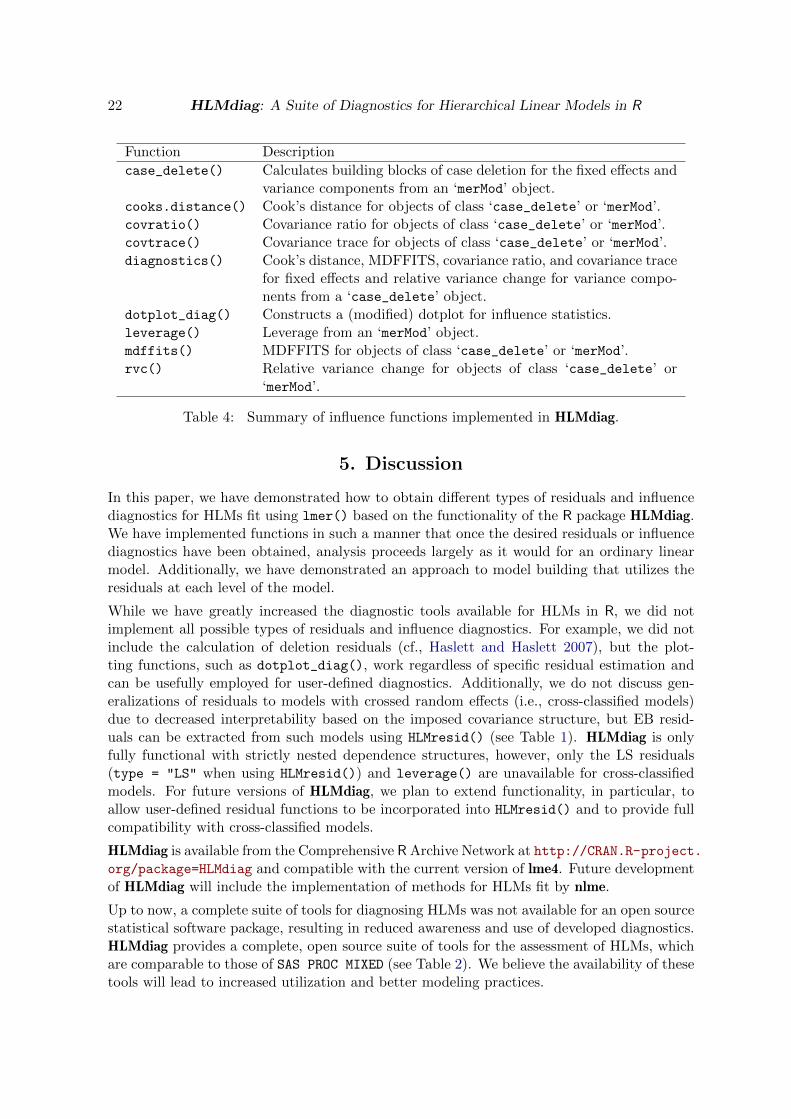
22 HLMdiag: A Suite of Diagnostics for Hierarchical Linear Models in R
Function Description
case_delete() Calculates building blocks of case deletion for the fixed effects andvariance components from an ‘merMod’ object.
cooks.distance() Cook’s distance for objects of class ‘case_delete’ or ‘merMod’.covratio() Covariance ratio for objects of class ‘case_delete’ or ‘merMod’.covtrace() Covariance trace for objects of class ‘case_delete’ or ‘merMod’.diagnostics() Cook’s distance, MDFFITS, covariance ratio, and covariance trace
for fixed effects and relative variance change for variance compo-nents from a ‘case_delete’ object.
dotplot_diag() Constructs a (modified) dotplot for influence statistics.leverage() Leverage from an ‘merMod’ object.mdffits() MDFFITS for objects of class ‘case_delete’ or ‘merMod’.rvc() Relative variance change for objects of class ‘case_delete’ or
‘merMod’.
Table 4: Summary of influence functions implemented in HLMdiag.
5. Discussion
In this paper, we have demonstrated how to obtain different types of residuals and influencediagnostics for HLMs fit using lmer() based on the functionality of the R package HLMdiag.We have implemented functions in such a manner that once the desired residuals or influencediagnostics have been obtained, analysis proceeds largely as it would for an ordinary linearmodel. Additionally, we have demonstrated an approach to model building that utilizes theresiduals at each level of the model.
While we have greatly increased the diagnostic tools available for HLMs in R, we did notimplement all possible types of residuals and influence diagnostics. For example, we did notinclude the calculation of deletion residuals (cf., Haslett and Haslett 2007), but the plot-ting functions, such as dotplot_diag(), work regardless of specific residual estimation andcan be usefully employed for user-defined diagnostics. Additionally, we do not discuss gen-eralizations of residuals to models with crossed random effects (i.e., cross-classified models)due to decreased interpretability based on the imposed covariance structure, but EB resid-uals can be extracted from such models using HLMresid() (see Table 1). HLMdiag is onlyfully functional with strictly nested dependence structures, however, only the LS residuals(type = "LS" when using HLMresid()) and leverage() are unavailable for cross-classifiedmodels. For future versions of HLMdiag, we plan to extend functionality, in particular, toallow user-defined residual functions to be incorporated into HLMresid() and to provide fullcompatibility with cross-classified models.
HLMdiag is available from the Comprehensive R Archive Network at http://CRAN.R-project.org/package=HLMdiag and compatible with the current version of lme4. Future developmentof HLMdiag will include the implementation of methods for HLMs fit by nlme.
Up to now, a complete suite of tools for diagnosing HLMs was not available for an open sourcestatistical software package, resulting in reduced awareness and use of developed diagnostics.HLMdiag provides a complete, open source suite of tools for the assessment of HLMs, whichare comparable to those of SAS PROC MIXED (see Table 2). We believe the availability of thesetools will lead to increased utilization and better modeling practices.
Journal of Statistical Software 23
Acknowledgments
The authors would like to thank the associate editor and reviewers whose comments andsuggestions substantially improved the paper.
References
Bates D, Maechler M, Bolker B (2013a). lme4: Linear Mixed-Effects Models Using S4 Classes.R package version 1.0-5, URL http://CRAN.R-project.org/package=lme4.
Bates D, Maechler M, Bolker B (2013b). mlmRev: Examples from Multilevel ModellingSoftware Review. R package version 1.0-5, URL http://CRAN.R-project.org/package=
mlmRev.
Belsley DA, Kuh E, Welsch RE (1980). Regression Diagnostics: Identifying Influential Dataand Sources of Collinearity. John Wiley & Sons, New York.
Buja A, Cook D, Hofmann H, Lawrence M, Lee EK, Swayne DF, Wickham H (2009). “Sta-tistical Inference for Exploratory Data Analysis and Model Diagnostics.” PhilosophicalTransactions of the Royal Society A: Mathematical, Physical and Engineering Sciences,367(1906), 4361–4383.
Christensen R, Pearson L, Johnson W (1992). “Case-Deletion Diagnostics for Mixed Models.”Technometrics, 34(1), 38–45.
Cook RD, Weisberg S (1982). Residuals and Influence in Regression. Chapman and Hall,New York.
Demidenko E (2004). Mixed Models: Theory and Applications. John Wiley & Sons, Hoboken.
Demidenko E, Stukel TA (2005). “Influence Analysis for Linear Mixed-Effects Models.” Statis-tics in Medicine, 24(6), 893–909.
Dillane D (2005). Deletion Diagnostics for the Linear Mixed Model. Ph.D. thesis, TrinityCollege, Dublin.
Eddelbuettel D, Sanderson C (2014). “RcppArmadillo: Accelerating R with High-PerformanceC++ Linear Algebra.” Computational Statistics & Data Analysis, 71, 1054–1063.
Ghidey W, Lesaffre E, Eilers P (2004). “Smooth Random Effects Distribution in a LinearMixed Model.” Biometrics, 60(4), 945–953.
Ghidey W, Lesaffre E, Verbeke G (2010). “A Comparison of Methods for Estimating theRandom Effects Distribution of a Linear Mixed Model.” Statistical Methods in MedicalResearch, 19(6), 575–600.
Goldstein H (2011). Multilevel Statistical Models. 4th edition. John Wiley & Sons, Chichester.
Goldstein H, Carpenter J, Kenward M, Levin K (2009). “Multilevel Models with MultivariateMixed Response Types.” Statistical Modelling, 9(3), 173–197.

24 HLMdiag: A Suite of Diagnostics for Hierarchical Linear Models in R
Goldstein H, Rasbash J, Yang M, Woodhouse G, Pan H, Nuttall D, Thomas S (1993). “AMultilevel Analysis of School Examination Results.” Oxford Review of Education, 19(4),425–433.
Gurka MJ, Edwards LJ, Muller KE, Kupper LL (2006). “Extending the Box-Cox Transfor-mation to the Linear Mixed Model.” Journal of the Royal Statistical Society A, 169(2),273–288.
Haslett J, Haslett SJ (2007). “The Three Basic Types of Residuals for a Linear Model.”International Statistical Review, 75(1), 1–24.
Hedeker D, Gibbons R, Toit SD, Patterson D (2008). SuperMix: A Program for Mixed-Effects Regression Models. Scientific Software International, Chicago. URL http://www.
ssicentral.com/supermix/.
Hilden-Minton J (1995). Multilevel Diagnostics for Mixed and Hierarchical Linear Models.Ph.D. thesis, University of California Los Angeles.
Hox JJ (2010). Multilevel Analysis: Techniques and Applications. 2nd edition. Routledge,New York.
Kreft I, de Leeuw J (1998). Introducing Multilevel Modeling. Sage, London.
Langford I, Lewis T (1998). “Outliers in Multilevel Data.” Journal of the Royal StatisticalSociety A, 161(2), 121–160.
Leckie G, Charlton C (2013). “runmlwin: A Program to Run the MLwiN Multilevel ModelingSoftware from within Stata.” Journal of Statistical Software, 52(11), 1–40. URL http:
//www.jstatsoft.org/v52/i11/.
Loy A, Hofmann H (2013). “Diagnostic Tools for Hierarchical Linear Models.” Wiley Inter-disciplinary Reviews: Computational Statistics, 5(1), 48–61.
McCulloch CE, Searle SR (2001). Generalized, Linear, and Mixed Models. John Wiley &Sons, New York.
Nieuwenhuis R, Pelzer B, te Grotenhuis M (2013). influence.ME: Tools for DetectingInfluential Data in Mixed Effects Models. R package version 0.9-3, URL http://CRAN.
R-project.org/package=influence.ME.
Nieuwenhuis R, te Grotenhuis M, Pelzer B (2012). “influence.ME: Tools for Detecting Influ-ential Data in Mixed Effects Models.” The R Journal, 4(2), 38–47.
Nobre JS, Singer JM (2011). “Leverage Analysis for Linear Mixed Models.” Journal of AppliedStatistics, 38(5), 1063–1072.
Pinheiro J, Bates D, DebRoy S, Sarkar D, R Core Team (2013). nlme: Linear and NonlinearMixed Effects Models. R package version 3.1-113, URL http://CRAN.R-project.org/
package=nlme.
Pinheiro J, Liu C, Wu Y (2001). “Efficient Algorithms for Robust Estimation in LinearMixed-Effects Models Using the Multivariate t-Distribution.” Journal of Computationaland Graphical Statistics, 10(2), 249–276.

Journal of Statistical Software 25
Pinheiro JC, Bates DM (2000). Mixed-Effects Models in S and S-PLUS. Springer-Verlag, NewYork.
Rabe-Hesketh S, Skrondal A, Pickles A (2004). “gllamm Manual.” Technical Report 160,University of California Berkley, Division of Biostatistics. URL http://www.bepress.
com/ucbbiostat/paper160.
Rasbash J, Steele F, Browne WJ, Goldstein H (2012). A User’s Guide to MLwiN, v2.26.Centre for Multilevel Modelling, University of Bristol.
Raudenbush SW, Bryk AS (2002). Hierarchical Linear Models: Applications and Data Anal-ysis Methods. 2nd edition. Sage, Thousand Oaks.
Raudenbush SW, Bryk AS, Cheong YF, Condon RT, du Toit M (2011). HLM 7: HierarchicalLinear and Nonlinear Modeling. Scientific Software International, Lincolnwood.
R Core Team (2013). R: A Language and Environment for Statistical Computing. R Foun-dation for Statistical Computing, Vienna, Austria. ISBN 3-900051-07-0, URL http:
//www.R-project.org/.
Sanderson C (2010). “Armadillo: An Open Source C++ Linear Algebra Library for FastPrototyping and Computationally Intensive Experiments.” Technical report, NICTA. URLhttp://arma.sourceforge.net.
SAS Institute Inc (2008). SAS/STAT Software, Version 9.2. Cary, NC. URL http://www.
sas.com/.
Schabenberger O (2004). “Mixed Model Influence Diagnostics.” In Proceedings of the Twenty-Ninth Annual SAS® Users Group International Conference. SAS Institute Inc, Cary, NC.Paper 189–29.
Shen W, Louis TA (1999). “Empirical Bayes Estimation via the Smoothing by RougheningApproach.” Journal of Computational and Graphical Statistics, 8(4), 800–823.
Shi L, Chen G (2008). “Case Deletion Diagnostics in Multilevel Models.” Journal of Multi-variate Analysis, 99(9), 1860–1877.
Snijders T, Berkhof J (2008). “Diagnostic Checks for Multilevel Models.” In J de Leeuw,E Meijer (eds.), Handbook of Multilevel Analysis, chapter 3, pp. 141–175. Springer-Verlag,New York.
Snijders TAB, Bosker RJ (2012). Multilevel Analysis: An Introduction to Basic and AdvancedMultilevel Modeling. 2nd edition. Sage, London.
StataCorp (2007). Stata 10 Longitudinal/Panel Data Reference Manual. Stata Press, CollegeStation.
Staudenmayer J, Lake E, Wand M (2009). “Robustness for General Design Mixed Modelsusing the t-Distribution.” Statistical Modelling, 9(3), 235.

26 HLMdiag: A Suite of Diagnostics for Hierarchical Linear Models in R
Tremblay A, Ransijn J (2013). LMERConvenienceFunctions: A Suite of Functionsto Back-Fit Fixed Effects and Forward-Fit Random Effects, as well as Other Miscella-neous Functions. R package version 2.1, URL http://CRAN.R-project.org/package=
LMERConvenienceFunctions.
Tukey JW (1977). Exploratory Data Analysis. Addison Wesley, Reading.
Verbeke G, Lesaffre E (1996). “A Linear Mixed-Effects Model with Heterogeneity in theRandom-Effects Population.” Journal of the American Statistical Association, 91(433),217–221.
Verbeke G, Lesaffre E (1997). “The Effect of Misspecifying the Random-Effects Distributionin Linear Mixed Models for Longitudinal Data.” Computational Statistics & Data Analysis,23(4), 541–556.
West BT, Galecki AT (2011). “An Overview of Current Software Procedures for Fitting LinearMixed Models.” The American Statistician, 65(4), 274–282.
Wickham H (2009). ggplot2: Elegant Graphics for Data Analysis. Springer-Verlag, NewYork. URL http://had.co.nz/ggplot2/book.
Wickham H (2012). nullabor: Tools for Graphical Inference. R package version 0.2.1, URLhttp://CRAN.R-project.org/package=nullabor.
Yuan KH, Bentler PM (2002). “On Normal Theory Based Inference for Multilevel Modelswith Distributional Violations.” Psychometrika, 67(4), 539–561.
Zewotir T (2008). “Multiple Cases Deletion Diagnostics for Linear Mixed Models.” Commu-nications in Statistics – Theory and Methods, 37(7), 1071–1084.
Zhang D, Davidian M (2001). “Linear Mixed Models with Flexible Distributions of RandomEffects for Longitudinal Data.” Biometrics, 57(3), 795–802.

Journal of Statistical Software 27
A. Graphical inference for model diagnostics
In this paper we use the idea of the lineup protocol introduced by Buja et al. (2009) to assessmodel assumptions for the HLM. More specifically, we use this protocol to judge whetherthe assumption of constant error variance of the level-1 residuals across standLRT2 is valid.To conduct this visual test, we generate 19 null plots against which the true data will becompared by simulating from the model and obtaining the residuals.
First, we simulate null data sets, refit the models, and calculate the residuals:
R> sim_fm2 <- simulate(fm2, nsim = 19)
R> refit_fm2 <- apply(sim_fm2, 2, refit, object = fm2)
R> sim_fm2_lev1_resid <- ldply(refit_fm2, function(x){
+ HLMresid(object = x, level = 1, type = "LS", sim = x@resp$y,
+ standardize = "semi")
+ })
Next, we relabel the data frame for use with the nullabor package (Wickham 2012):
R> sim_fm2_lev1_resid$.n <- rep(1:19, each = 4059)
R> names(sim_fm2_lev1_resid)[4:5] <- c("standLRT2", "standLRT3")
In R the lineup is easily obtained using the lineup() function. First we format the dataframe
R> lev1_resid_fm2 <- HLMresid(object = fm2, level = 1, type = "LS",
+ standardize = "semi")
R> names(lev1_resid_fm2)[3:4] <- c("standLRT2", "standLRT3")
R> class(lev1_resid_fm2[,3]) <- "numeric"
Next, we create the lineup:
R> qplot(standLRT2, semi.std.resid, data = lev1_resid_fm2,
+ geom = "point", alpha = I(0.3)) %+%
+ lineup(true = lev1_resid_fm2, samples = sim_fm2_lev1_resid) +
+ facet_wrap(~ .sample, ncol = 4) +
+ geom_hline(aes(yintercept = 0), colour = I("red")) +
+ ylab("semi-standardized residuals")
Figure 3 displays the resulting lineup. The true plot is shown in panel 19.
B. Session information
The output presented in this paper was obtained using the following session:
R> sessionInfo()
R version 3.0.2 (2013-09-25)
Platform: x86_64-apple-darwin10.8.0 (64-bit)
28 HLMdiag: A Suite of Diagnostics for Hierarchical Linear Models in R
locale:
[1] en_US.UTF-8/en_US.UTF-8/en_US.UTF-8/C/en_US.UTF-8/en_US.UTF-8
attached base packages:
[1] stats graphics grDevices utils datasets methods
[7] base
other attached packages:
[1] mgcv_1.7-27 nlme_3.1-113 ggplot2_0.9.3.1 plyr_1.8
[5] nullabor_0.2.1 HLMdiag_0.2.4 lme4_1.0-5 Matrix_1.1-0
[9] lattice_0.20-24
loaded via a namespace (and not attached):
[1] colorspace_1.2-4 dichromat_2.0-0 digest_0.6.3
[4] grid_3.0.2 gtable_0.1.2 labeling_0.2
[7] MASS_7.3-29 minqa_1.2.1 munsell_0.4.2
[10] proto_0.3-10 RColorBrewer_1.0-5 reshape2_1.2.2
[13] scales_0.2.3 splines_3.0.2 stats4_3.0.2
[16] stringr_0.6.2 tools_3.0.2
Affiliation:
Adam LoyDepartment of MathematicsLawrence UniversityAppleton, WI 54911, United States of AmericaE-mail: [email protected]: http://adamloy.com/
Heike HofmannDepartment of StatisticsIowa State UniversityAmes, IA 50011-1210, United States of AmericaE-mail: [email protected]: http://www.public.iastate.edu/~hofmann/
Journal of Statistical Software http://www.jstatsoft.org/
published by the American Statistical Association http://www.amstat.org/
Volume 56, Issue 5 Submitted: 2012-04-15January 2014 Accepted: 2013-04-24