Historical Social ResearchHistorische Sozialforschung

No. 155HSR Vol. 41 (2016) 1

Special Issue

Peter Itzen & Simone M. Müller (Eds.)

Risk as an Analytical Category:Selected Studies in the Social History

of the Twentieth Century

Mixed Issue

Articles

The Journal: Editorial Board Main Editors Heinrich Best (Jena), Wilhelm H. Schröder (Cologne) Managing Editors Wilhelm H. Schröder, In-Chief (Cologne), Nina Baur (Berlin), Heinrich Best (Jena), Rainer Diaz-Bone (Lucerne), Philip J. Janssen (Cologne), Johannes Marx (Bamberg) Co-operating Editors Frank Bösch (Potsdam), Onno Boonstra (Nijmegen), Joanna Bornat (London), Franz Breuer (Münster), Leen Breure (Utrecht), Christoph Classen (Potsdam), Jürgen Danyel (Potsdam), Bert De Munck (Antwerp), Claude Didry (Paris), Claude Diebolt (Strasbourg), Georg Fertig (Halle), Gudrun Gersmann (Cologne), Karen Hagemann (Chapel Hill, NC), M. Michaela Hampf (Berlin), Rüdiger Hohls (Berlin), Jason Hughes (Leicester), Ralph Jessen (Cologne), Claire Judde de Larivière (Toulouse), Günter Mey (Magdeburg), Jürgen Mittag (Cologne), Katja Mruck (Berlin), Dieter Ohr (Berlin), Kai Ruffing (Cas-sel), Patrick Sahle (Cologne), Kevin Schürer (Leicester), Jürgen Sensch (Cologne), Manfred Thaller (Cologne), Paul W. Thurner (Munich), Roland Wenzlhuemer (Heidel-berg), Jens O. Zinn (Melbourne) Consulting Editors Erik W. Austin (Ann Arbor), Francesca Bocchi (Bologna), Leonid Borodkin (Moscow), Gerhard Botz (Vienna), Christiane Eisenberg (Berlin), Josef Ehmer (Vienna), Richard J. Evans (Cambridge), Jürgen W. Falter (Mainz), Harvey J. Graff (Columbus, OH), Arthur E. Imhof (Berlin), Konrad H. Jarausch (Chapel Hill, NC), Eric A. Johnson (Mt. Pleasant, MI), Hartmut Kaelble (Berlin), Hans Mathias Kepplinger (Mainz), Jürgen Kocka (Ber-lin), John Komlos (Munich), Jean-Paul Lehners (Luxembourg), Jan Oldervoll (Bergen), Eva Österberg (Lund), Janice Reiff (Los Angeles), Ernesto A. Ruiz (Florianopolis), Martin Sabrow (Potsdam), Rick Trainor (Oxford), Louise Tilly (New York), Jürgen Wilke (Mainz)

CONTENTS

HSR 41 (2016) 1 │ 3

Special Issue: Risk & Social History Introduction Peter Itzen & Simone M. Müller 7

Risk as a Category of Analysis for a Social History of the Twentieth Century: An Introduction.

Contributions Arwen P. Mohun 30

Constructing the History of Risk. Foundations, Tools, and Reasons Why.

Stefan Kaufmann & Ricky Wichum 48 Risk and Security: Diagnosis of the Present in the Context of (Post-)Modern Insecurities.

Malte Thießen 70 Risk as a Resource: On the Interplay between Risks, Vaccinations and Welfare States in Nineteenth- and Twentieth-Century Germany.

Jörg Arnold 91 “The Death of Sympathy.” Coal Mining, Workplace Hazards, and the Politics of Risk in Britain, ca. 1970-1990.

Sebastian Haus 111

Risky Sex – Risky Language. HIV/AIDS and the West German Gay Scene in the 1980s.

Kai Nowak 135 Teaching Self-Control. Road Safety and Traffic Education in Postwar Germany.

Peter Itzen 154

Who is Responsible in Winter? Traffic Accidents, the Fight against Hazardous Weather and the Role of Law in a History of Risks.

Meike Haunschild 176 Freedom versus Security. Debates on Social Risks in Western Germany in the 1950s.

Sarah Haßdenteufel 201 Covering Social Risks. Poverty Debate and Anti-Poverty Policy in France in the 1980s.

HSR 41 (2016) 1 │ 4

Felix Krämer 223 Hazards of Being a Male Breadwinner: Deadbeat Dads in the United States of the 1980s.

Nicolai Hannig 240 The Checkered Rise of Resilience. Anticipating Risks of Nature in Switzerland and Germany since 1800.

Simone M. Müller 263 “Cut Holes and Sink ‘em”: Chemical Weapons Disposal and Cold War History as a History of Risk.

Mixed Issue: Articles Shiping Tang 287

Eurasia Advantage, not Genetic Diversity: Against Ashraf and Galor’s “Genetic Diversity” Hypothesis.

Inge Marszolek & Yvonne Robel 328

The Communicative Construction of Collectivities: An Interdisciplinary Approach to Media History.

Historical Social Research 41 (2016) 1, 287-327 │© GESIS DOI: 10.12759/hsr.41.2016.1.287-327

Eurasia Advantage, not Genetic Diversity: Against Ashraf and Galor’s “Genetic Diversity” Hypothesis

Shiping Tang ∗

Abstract: »Nicht genetische Vielfalt, sondern Vorteil Eurasiens. Gegen Ashraf und Galors „Genetic Diversity“-Hypothese«. Ashraf and Galor (2012) advanced the bold thesis that genetic diversity within different human populations has been a foundational determinant of long-run economic development. We show that their results are not robust after controlling for a key missing variable – the Eurasia dummy. After controlling for the Eurasia dummy, all indicators of genetic diversity lose statistical significance in regressions with indicators of economic development as dependent variables. Ashraf and Galor’s statistical results merely “reflect” – literally – Eurasia’s unique advantage in supporting economic development that was mostly based on settled agriculture until about AD1500. Keywords: Eurasia Advantage, Jared Diamond, genetic diversity, economic de-velopment.

1. Introduction: Is Economic Development within our Genetic Diversity?1

Ashraf and Galor (2012) advanced the bold thesis that genetic diversity within different human populations has been a more foundational determinant of eco-nomic development in the long run than geography, from the dawn of our spe-cies to today (Ashraf and Galor 2012, 1, 8-9).2 If the theory and the evidences ∗ Shiping Tang, School of International Relations and Public Affairs (SIRPA), Fudan Univeristy,

220 Han-dan Road, Shanghai, 200433, China; twukong@fudan.edu.cn. 1 This article is dedicated to Jared Diamond and his Guns, Germs, and Steel.

For critical discussions and comments, the author thanks Shuo Chen, Jared Diamond, Min Tang, Dwayne Woods, Yu Zheng, the two reviewers of this journal, and an economist who wishes to remain anonymous. Andi Wang provided excellent research assistance. This re-search is supported by a “985 project” 3rd phase bulk grant from Fudan University to the author.

2 For the sake of completeness and convenience, we rely on their working paper version, denoted as Ashraf and Galor (2012). The published version of their paper is cited as Ashraf and Galor (2013a). Although Ashraf and Galor (2012, 2013a) used the term “the Out of Afri-ca Thesis” in their titles, their core explanatory variable is really “genetic diversity.” I thus use “Genetic Diversity Hypothesis” in my critique of them to avoid the impression that I am against the original “Out of Africa Hypothesis” in the field of human evolution. In fact, I

HSR 41 (2016) 1 │ 288

presented by Ashraf and Galor (2012) hold, Ashraf and Galor (2012) surely represent a major advancement in our understanding of the deep causes of economic development in the long run, and Ashraf and Galor certainly did not understate the potential significance of their finding a bit (ibid., 8-9).

Nowadays, anything that claims to link any aspect of human genetics with human social behavior and/or macro social outcomes is bound to garner atten-tion from the scientific community and the general public. Unsurprisingly, even before Ashraf and Galor’s (2012) working paper was to be published as the lead article in American Economic Review (Ashraf and Galor 2013a), their provocative findings were picked by both a Science newspiece (Chin 2012) and a Nature commentary (Calloway 2012). Eventually, a mini-firestorm in the internet space resulted, partly ignited by a strongly worded critique from a group of anthropologists (Guedes et al. 2013; for other scientists’ reactions, see Calloway 2012).3

So far, however, much of the criticism directed against Ashraf and Galor (2012), especially the critique by Guedes, et al. (2013), has been more political and ethical than scientific (Gelman 2013, 46). More prominently, without re-analyzing Ashraf and Galor’s (2012) data and results, Guedes et al. (2013, 77) asserted:

Ashraf and Galor’s (2013) paper is based on a fundamental scientific misunder-standing, bad data, poor methodology, and an uncritical theoretical framework […] this study has the potential to cause serious harm (emphasis added).4

As such, Ashraf and Galor can easily dismiss their critics as largely political and unscientific and then claim “the scientific and even moral high ground” for themselves, as Gelman (2013, 46) drily noted. Indeed, in their reply to Guedes et al. (2013), Ashraf and Galor (2013b, 1) retorted exactly as such:

these criticisms [i.e., Guedes et al. 2013] are scientifically baseless and ulti-mately reflective of a misunderstanding of our empirical methodology, poten-tial unfamiliarity with the statistical techniques that we employ, and a misin-

strongly support the original “Out of Africa Hypothesis” in the field of human evolution, just as Diamond (1997) does.

3 See the exchanges on a website maintained by Jason Collins <www.jasoncollins.org> and another website maintained by Matter Zimmerman <www.biasedtransmission.blogspot. com> (Accessed September 16, 2013).

4 See also a blog by another anthropologist, Rebecca Dean, “Look what the economists do with human diversity data” <www.rebeccamdean.blogspot> (Accessed September 16, 2013). The only place where Guedes et al. (2013) came close to do so has been their pointing out that a few historical data points of population density, mostly from the Americas, might have been mis-measured by Ashraf and Galor (2012), following McEvedy and Jones (1978). Yet, Guedes et al. (2013) did not test whether better measurements of these data points will significantly change Ashraf and Galor’s (2012) results at all. As shown in section four below, leaving the Americas out (i.e., the sample with only the Old World) does not significantly change the statistical results.

HSR 41 (2016) 1 │ 289

terpretation of our findings (emphasis added; the same retort is essentially re-peated on page 4 of their response).

In this contribution, we provide a systematic econometric rebuttal against Ashraf and Galor, based on Ashraf and Galor’s (2012) own data. We do not question the possible link between migratory distance and predicted genetic diversity: We give Ashraf and Galor the benefit of doubt that migratory distance is a good proxy for predicted genetic diversity. Neither do we challenge the link between genetic diversity and innovation or the link between genetic diversity and cooper-ation/conflict, although we do wish to note that the case presented by Ashraf and Galor (2012) on these two possible causal links has been weak at best. The evi-dences presented by Ashraf and Galor (2012) are not from studies of human groups or even primates; rather, they are from flies, spiders, and honeybees.5 Finally, we do not even challenge the data collected by Ashraf and Galor: We assume that all of their data are valid and accurate.6 Instead, we attempt to un-ambiguously show that even with their own data, Ashraf and Galor’s (2012) results cannot hold after controlling for a key variable that is missing in their inquiry. Put it differently, Ashraf and Galor’s (2012) results are an artifact of leaving out a key variable that should have been controlled. As such, Ashraf and Galor’s conclusions are on shaky ground, if not entirely unwarranted.

A key caveat is in order here. In some of the regressions reported below, the number of countries (as observations) is different from what Ashraf and Galor (2012) originally reported. This is not due to our using a different set of coun-tries. Indeed, the original Ashraf and Galor (2012) dataset contains 208 coun-tries, and the reason why regressions reported in Ashraf and Galor (2012) have fewer countries than the regressions reported below is because many of the independent variables they deploy have many missing values. In contrast, be-cause we restrict our independent variables to several exogenous geographical variables and these variables have fewer missing data points, the number of countries in most of our regressions is larger than the number of countries reported by Ashraf and Galor (2012). The fact that our regressions have more countries than regressions reported by Ashraf and Galor (2012), however, does not invalidate our challenges against Ashraf and Galor (2012). This is so be-cause when the Eurasia dummy is not controlled, we obtain almost identical results as Ashraf and Galor (2012) did: Various indicators of genetic diversity 5 Jason Collins has provided well-informed comments on these and other related issues in his

blogspace: <www.jasoncollins.org>. See also the comments by Matt Zimmerman on Ashraf and Galor (2012) at <www.biasedtransmission.blogspot.com> (Accessed September 16, 2013).

6 We, of course, readily admit that some of the data employed by Ashraf and Galor (2012), especially population density (PD) and rate of urbanization in pre-modern times, are sub-jected to serious problems of missing data and measurement error. For earlier discussions of the problems with data collected by McEvedy and Jones (1978) and Chandler (1987), see LeGates and Stout (1996, 21). See also Bandyopadhyay and Green (2012).

HSR 41 (2016) 1 │ 290

are statistically significant predictors of economic development and there seems to be a robust humped-shaped relation between genetic diversity and economic development. Yet, once the Eurasia dummy is controlled, various indicators of genetic diversity lose their statistical significance in almost all the regressions and the supposedly robust humped-shaped relation vanishes.

The rest of our paper is structured as follows. Section two provides a brief recount of Ashraf and Galor’s (2012) key arguments, data, methods, and re-sults. Section three presents our data and procedures for challenging Ashraf and Galor’s statistical results. Section four provides our results, showing that after controlling a key variable – the Eurasia dummy that is straight from Jared Diamond’s “Eurasia Advantage Thesis” (Diamond 1997) – the supposedly significant and robust effect on economic development of genetic diversity, however measured, disappears almost completely. We further show that our results are robust across different samples, using different indicators of eco-nomic development as dependent variables, and using different indicators of genetic diversity as independent variables. Building upon existing empirical testing of the Diamond Thesis (e.g. Olsson and Hibbs 2005; Putterman 2008; Petersen and Skaaning 2010), section five establishes the validity of Diamond’s “Eurasia Advantage Thesis” more systematically. Section six provides a highly plausible explanation for Ashraf and Galor’s (2012) misleading results and conclusions. A brief conclusion follows.

2. Ashraf and Galor (2012): Key Arguments, Data, Methods, and Results

Ashraf and Galor (2012, 1-2) nicely summarized the central thesis and key prediction of their paper, quoted in full below, with their key empirical predic-tions emphasized in italics.

The hypothesis rests upon two fundamental building blocks. First, migratory distance from the cradle of humankind in East Africa had an adverse effect on the degree of genetic diversity within ancient indigenous settlements across the globe. Following the prevailing hypothesis, commonly known as the serial founder effect, it is postulated that, in the course of human expansion over planet Earth, as subgroups of the populations of parental colonies left to estab-lish new settlements further away, they carried with them only a subset of the overall genetic diversity of their parental colonies. Second, there exists an optimal level of diversity for economic development, reflecting the interplay between the opposing effects of diversity on the devel-opment process. The adverse effect pertains to the detrimental impact of di-versity on the efficiency of the aggregate production process. Heterogeneity raises the likelihood of disarray and mistrust, reducing cooperation and dis-rupting the socioeconomic order. Higher diversity is therefore associated with lower productivity, which inhibits the capacity of the economy to operate effi-

HSR 41 (2016) 1 │ 291

ciently relative to its production possibility frontier. The beneficial effect of diversity, on the other hand, concerns the positive role of heterogeneity in the expansion of society’s production possibility frontier. A wider spectrum of traits is more likely to contain those that are complementary to the advance-ment and successful implementation of superior technological paradigms. Higher diversity therefore enhances society’s capability to integrate advanced and more efficient production methods, expanding the economy’s production possibility frontier and conferring the benefits of improved productivity. Higher diversity in a society’s population can therefore have conflicting ef-fects on the level of its productivity. Aggregate productivity is enhanced on the one hand by an increased capacity for technological advancement while diminished on the other by reduced cooperation and efficiency. However, if the beneficial effects of population diversity dominate at lower levels of diver-sity and the detrimental effects prevail at higher ones (i.e., if there are dimin-ishing marginal returns to both diversity and homogeneity), the theory would predict a hump-shaped effect of genetic diversity on productivity throughout the development process.

To substantiate their thesis, Ashraf and Galor (2012) first established that mi-gratory distance from (Addis Ababa) Ethiopia does have an inverse relationship with observed genetic diversity, using a small dataset from 53 ethnic groups across globe constructed by Ramachandran et al. (2005, as Figure 1 in Ashraf and Galor 2012, 2). Ashraf and Galor then went on to establish that even within this limited sample, observed genetic diversity has a robust and statistically significant hump-shaped relationship with population density of their respec-tive countries at AD1500 (Ashraf and Galor 2012, 18-24, esp., Tables 1 and 2, and Figure 3).

After this reassuring start, Ashraf and Galor then went on to build a dataset on migratory distance of human populations from (Addis Ababa) Ethiopia to their present capital city and used this measure to predict “genetic diversity” of different populations in today’s world (for the logic and methods for construct-ing “predicted genetic diversity,” see Ashraf and Galor 2012, 14-5).7 Eventual-ly, they constructed two measures of “predicted genetic diversity”: non-ancestry adjusted; ancestry-adjusted (by incorporating information on post-1500AD population flows, see Ashraf and Galor 2012, Appendix B, xiv-xvi

7 Ashraf and Galor’s (2012, 14-5) did not provide much rationale or information on how they

extrapolate from migratory distance to predicted genetic diversity. With a bit of statistical guesswork, however, we can reveal how Ashraf and Galor (2012) extrapolated from migra-tory distance to “predicted genetic diversity (pdiv).” For details, see Appendix A in: Shiping Tang, 2016, Online Appendix to: Eurasia Advantage, not Genetic Diversity: Against Ashraf and Galor’s “Genetic Diversity” Hypothesis, HSR Trans 28. doi: 10.12759/hsr.trans. 28.v01.2016. This volume of HSR Trans contains Appendices A-J.

HSR 41 (2016) 1 │ 292

and Appendix F, xl for details).8 These two indicators of predicted genetic diversity are then employed as key explanatory variables.

Ashraf and Galor’s (2012) key indicators of economic development include population density (hereafter, PD) at AD1, AD1000, AD1500 (McEvedy and Jones 1978), rate of urbanization at AD1500 (Chandler 1987; Modelski 2003; see also Bairoch 1988), and GDP per capita in 2000 (hereafter, GDPpc2000). These indicators of economic development are then deployed as key dependent varia-bles. With numerous tables and figures, Ashraf and Galor (2012) believed that they had shown that genetic diversity has a highly significant and hump-shaped relationship with economic development.9

3. Missing the Eurasia Continent: Logic, Data, and Procedure

In Guns, Germs, and Steel, Jared Diamond (1997) provided a sweeping account for the fate of human societies in the world up to AD1500 and how the pre-1500AD world has continued to shape the post-1500AD world.

Briefly, Diamond’s (1997) “Eurasia Advantage Thesis” argues that the Eur-asian continent as a whole holds some decisive advantages over all other conti-nents when it comes to providing the physical environment for economic devel-opment, at least until 1500AD. The Eurasia advantage has two core components. First, the Eurasia continent as a whole had been the home of most domesticated mammalian herbivores and omnivores (e.g., cow, goat, pig, and sheep) and staple crops (e.g., barley, millet, rice, and wheat). The Eurasia continent thus had “good material to work with” for developing settled agriculture (Olsson and Hibbs 2005, 913-8; see also Diamond 1997; Smith 1998; Petersen and Skaaning 2010, 205-7). Second, diffusion of domesticated animals and staple crops, together with other key agricultural technologies, has been easier on the Eurasia continent as a whole than other continents (e.g., Africa and the Americas) because

the spread of food production tended to occur more rapidly along east-west axes [e.g., within Eurasia] than along north-south axes [e.g., from Eurasia to Africa], mainly because locations at the same latitudes required less evolu-tionary change or adaptation of domesticates than did locations at different lat-itudes (Diamond 2002, 705; 1997; Petersen and Skaaning 2010, 207-10).10

8 Not surprisingly, these two measures are highly correlated (Pearson r=0.750, significant at

0.001 level). 9 Although Ashraf and Galor (2012) mostly used population density at AD1500 and

GDPpc2000 as dependent variables in their main text, they have also explored the relation-ships between genetic diversity and other indicators of economic development as depend-ent variables in their Appendix A (esp. Table A1, A2, A4, and A5).

10 We examine the second component of Diamond’s Thesis in more detail in section 5 below.

HSR 41 (2016) 1 │ 293

Because the Eurasia continent as a whole holds these two key advantages, it has been a more fertile ground for generating the First Economic Revolution or the Neolithic Revolution: the coming of settled agriculture. Because settled agriculture provided more stable sources of protein and staple corps, it provid-ed the key foundation for further economic development. This in turn resulted in a higher degree of urbanization and higher population density within a par-ticular geographical area (Olsson and Hibbs 2005). A higher degree of urbani-zation and population density in turn supported larger sociopolitical organiza-tions of people, eventually culminating in archaic states (Bockstette, Chanda and Putterman 2002; Putterman 2008; Borcan, Olsson, and Putterman 2014).11 Together, these earlier advantages in food production, weaponry technology, organizational skills in war-fighting, and immunity against certain infectious diseases would later allow people from the Eurasia continent to colonize other continents, including Africa, the Americas, and Oceania (Diamond 1997; Tang 2013, ch. 2).

In short, the “Eurasia Advantage thesis” argues that the Eurasian continent as a whole held some decisive advantages over all other continents when it comes to providing the physical environment for economic development, at least until 1500AD. After 1500AD, the Europeans began to colonize the world and brought what they had (good or bad) to the rest of the world. Along the way, the Europeans had thus vastly complicated the picture.

Because Ashraf and Galor (2012, 1, 8-9, Appendix A4, xi-xiii) explicitly set out to challenge the Diamond Thesis, Ashraf and Galor should have included Eurasia as a whole as a control dummy variable.12 Yet, they have failed to do. When this is the case, Ashraf and Galor’s (2012) results might have been the product of a failure to control for a key competing variable. We set out to test this possibility.

We proceed as follows: 1) We first test the Eurasia dummy (1 if a country is classified as a European or

an Asian countries in Ashraf and Galor’s own data; 0 otherwise) as a possi-ble independent explanatory factor for economic development against the four key indicators of economic development (i.e., PD at AD1, AD1000, AD1500, and GDPpc2000) as dependent variables, in three different sam-ples: the whole world, the whole world excluding Australia, Canada, New

11 Here, we are not concerned with whether earlier transition to settled agriculture and hence

statehood has a negative impact on subsequent political and economic development such as adoption of democracy and industrialization after 1500AD. For important works on this front, see Hariri (2012); Borcan, Olsson and Putterman (2014); Chanda, Cook and Putterman (2014). For a brief discussion, see the conclusion in Section 7.

12 We have also tested by inserting the Europe dummy and the Asia dummy separately into the regressions, and we obtain essentially identical results. These results are reported in sec-tion 4 below and in Appendix G.

HSR 41 (2016) 1 │ 294

Zealand, and the United States (hereafter, ACNU), and the Old World (i.e., Africa, Asia, plus Europe).13

2) We then test Ashraf and Galor’s key explanatory variables (genetic diversity or migratory distance, whether ancestry adjusted or not) separately and es-tablish their plausibility as key explanatory factors for long-run economic development. We test indicators of genetic diversity that are not ancestry-adjusted against all four key indicators of economic development, again in three different samples. Consistent with Ashraf and Galor’s logic, we only test ancestry adjusted measurements of predicted genetic diversity or migra-tory distance against PD1500 and GDPpc2000.14 Not surprisingly, in these regressions, we obtain results that are almost identical to the results reported in Ashraf and Galor (2012).

3) We then pit the Eurasia dummy against different indicators of genetic diver-sity in horse-race models, again within three different samples.

4) We then add more control variables. To avoid any possibility of endogenei-ty, we deploy only three fixed geographical variables: landlocked (1 if a country or territory is landlocked country, 0 if not), absolute latitude of a country (taking natural log), and island (1 if a country or territory is an is-land, 0 if not). We exclude other bio-climate variables such as area of arable land, rain fall, and soil PH etc., because they are subjected to modification by human activities and natural causes (Pimentel et al. 1995; Montgomery 2007).15 We also exclude other proxy indicators of economic development such as the timing of the Neolithic Revolution and ancient statehood as con-trol variables not only because archaeological dating the exact time of these events has never been easy and conclusive, but also because these indicators are intervening variables between Eurasia (and other exogenous geograph-ical variables) and economic development.

5) We then add distance to (regional) technological frontiers at AD1, AD1000, and AD1500 to the models in order to capture the effect of diffusion as sin-

13 The Eurasia dummy is easily generated by adding Ashraf and Galor’s Europe dummy and

Asia dummy together. Following Ashraf and Galor (2012), we also perform regressions with bootstrap procedures. Regression results with or without bootstrap procedures are almost identical. We thus report only results from regressions without bootstrap procedures here.

14 For the sake of completeness, we also regress ancestry-adjusted indicators of genetic diver-sity against PD1 and PD1000. These results are reported in the appendices of HSR Trans 28.

15 For instance, it is well known that the Fertile Crescent had become much less fertile in history partly due to human activities, especially agriculture supported by vast irrigation (Diamond 2011). Likewise, the pattern of rainfall has also changed significantly for northern China. Whereas the South China Sea monsoon could still reach much of northern China around 3000BC, today it can only reach the Yangtze valley (Liu 2004, ch. 2). Consequently, northern China has become much drier and less fertile. Moreover, data on rainfall, arable land etc. are all from contemporary time (i.e., post-1960), and surely we cannot use these data to explain outcomes before AD1500!

HSR 41 (2016) 1 │ 295

gled out by Diamond (1997). Data for these three variables are from Ashraf and Galor (2012).

6) We then test the effect upon economic development of genetic diversity vs. the three fixed geographical variables, within Eurasian countries alone. This is a litmus test whether genetic diversity has any impact upon economic de-velopment at all because the effect of Eurasia will be eliminated within this sub-sample of only Eurasian countries.

7) We then perform more robustness tests by inserting Europe and Asia into the models as two separate dummies, but always together. Again, various measures of genetic diversity have no robust relationship with economic de-velopment in these tests.

8) We then test Eurasia against genetic diversity in the limited samples of 21 countries with “observed” or “actual” genetic diversity to drive home our points. If “observed” genetic diversity has no robust significant relationship with economic development after controlling for the Eurasia dummy, then the whole enterprise of Ashraf and Galor’s (2012, esp. 18-24) has no foun-dation to start with and hence the whole enterprise collapses.

9) Because Ashraf and Galor (2012, Table D4, xxv) reported that letting differ-ent measurements of genetic diversity take natural log does not change their overall results, we also perform such tests by using the natural log of differ-ent measurements of genetic diversity as independent variables in various samples. Again, we obtain almost identical results that strongly contradict Ashraf and Galor’s claims. We report these results in the appendices of HSR Trans 28.

All estimations are based on a basic model below, following Ashraf and Galor (2012, 16-7):

ln(yi) = α + βGeneticdiversityi + γGeneticdiversityi2 + λZi + εi

Where iy is a measurement of economic development for country i (e.g., PD at AD1, AD1000, AD1500, or GDPpc2000), Geneticdiversity is the predicted genetic diversity of country i , iZ is a vector for control variables (e.g., the Eurasia dummy, distance to frontier at AD1, landlocked) for country i , and iεis an error term assumed to be normally distributed. Estimation procedures are standard OLS regressions as done by Ashraf and Galor (2012).

A caveat is in order. We drop rate of urbanization at 1500 (ur1500 in Ashraf and Galor 2012) as a dependent variable because it has far too many missing data points. We also drop other less direct indicators of economic development (e.g., the number of scientific articles published by a country divided by its population) or possible intervening variable between genetic diversity and economic development (e.g., trust) as dependent variables. After all, if genetic diversity is shown to have no robust and significant relationship with the four key indicators of economic development (i.e., PD at AD1, AD1000, AD1500, and GDPpc2000), the enterprise of Ashraf and Galor’s (2012) would have

HSR 41 (2016) 1 │ 296

collapsed completely, and there is little need for us to further test whether ge-netic diversity has any impact upon trust and numbers of scientific papers pub-lished when it comes to assessing the impact on economic development of genetic diversity.

We shall hold the following two straightforward predictions: 1) If Ashraf and Galor (2012) are correct, the hump-shaped relationship be-

tween indicators of (predicted) genetic diversity and various indicators of economic development should hold in most of the models with different sam-ples, even after controlling for the Eurasia dummy, the three other exogenous geographical variables, and distance to regional technological frontiers.

2) If, however, the Eurasia Advantage Thesis is correct, then the Eurasia dum-my should have a robust and significant positive relationship with various indicators of economic development whereas distance to regional technolog-ical frontiers should have a robust and significant negative relationship with various indicators of economic development, across most of the models with different samples. Moreover, the Eurasia dummy should replace various in-dicators of genetic diversity as the most potent explanatory factors for eco-nomic development in most horse-race models that pit the Eurasia dummy against various indicators of genetic diversity, in different samples.

4. Missing the Big Eurasia Continent: Empirical Results

4.1 Initial Test: Establishing the Plausibility of the Diamond Thesis

Our initial test firmly establishes the Eurasia dummy as a plausible key explan-atory factor for economic development, lending strong support for the first key component of “the Diamond Thesis” (see also Olsson and Hibbs 2005; Putter-man 2008; Petersen and Skaaning 2010). As shown in Table 1, the Eurasia dummy is highly significant in all the models when tested independently against all four key indicators of economic development as dependent variable in the three different samples at a level of p<0.001 (t statistics from 4.823 to 8.543). Indeed, the Eurasia dummy alone can explain 11.4%-32% of the varia-tions with the four indicators of economic development.

We then test the unconditional effect on economic development of two measures of genetic diversity. As shown in Table 2A and Table 2B, when tested independently, indicators of genetic diversity, whether ancestry-adjusted or not, are significant in most of the models in all three different samples (see also Table A3-a, and A4-a). Moreover, the signs in front of the first order term and the second order term, when they are significant, are consistent with Ashraf and Galor’s thesis: the first order term has a positive sign whereas the second order term has a negative sign. Furthermore, consistent with the results report-ed in Tables 5, 6, 7, D9, and D11 in Ashraf and Galor (2012), predicted genetic

HSR 41 (2016) 1 │ 297

diversity-ancestry adjusted is significant when GDPpc2000 is the dependent variable but insignificant when the dependent variable is indicator of economic development before AD1500. These initial results are broadly consistent with Ashraf and Galor’s thesis that genetic diversity has a hump-shaped relationship with economic development (e.g., Ashraf and Galor 2012, Figures 3, 4, and 5).

One should note, however, that Ashraf and Galor’s results do not always hold in these initial tests. For instance, in Model 10 and Model 11 of Table 2A, neither the first order term nor the second order term of predicted genetic di-versity is significant when PD1000 and PD1500 are the dependent variables and the sample is the Old World. Moreover, in Model 6 of Table 2B, both the first order term and the second order tem of predicted genetic diversity-ancestry adjusted are significant when PD1000 is the dependent variable and the sample is the whole world excluding ACNU. Likewise, in Model 9 of Table 2B, both the first order term and the second order tem of predicted genetic diversity-ancestry adjusted are significant when PD1 is the dependent variable and the sample is the Old World. Yet according to Ashraf and Galor (2012), indicators of predicted genetic diversity-ancestry adjusted should be largely irrelevant for understanding outcomes before AD1500. These initial results, however, provide at least some support for Ashraf and Galor’s (2012) claim that genetic diversity is a significant determining factor of economic develop-ment, if not one hundred percent.

4.2 Horse-Race Models: The Eurasia Advantage Demolishes “Genetic Diversity”

Once we pit the Eurasia dummy against different measures of genetic diversity, however, things fall apart almost completely for Ashraf and Galor’s thesis that genetic diversity has a robust and significant hump-shaped relationship with economic development. Strikingly, once we put both predicted genetic diversi-ty and the Eurasia dummy together into regressions, whereas the Eurasia dum-my remains highly significant throughout, predicted genetic diversity – whether its first order term or its second order term – becomes thoroughly insignificant (Table 3A). Moreover, these results are robust when we add more exogenous control variables, including the three fixed geographical variables and distance to regional technological frontiers at different historical time (Table 3B). Also, inserting the two terms of predicted genetic diversity into the models does not improve the overall fit of the models with only the Eurasia dummy (compare Models 1-4 of Table 3A with Models 9-12 of Table 3A). In contrast, inserting the three fixed geographical variables and the distance to regional technological frontiers at different historical time into the models does improve the overall fit of the models significantly (compare Table 3A and Table 3B).

We obtain almost identical results when employing predicted genetic diver-sity-ancestry adjusted as the indicator of genetic diversity (Table 4A and Table

HSR 41 (2016) 1 │ 298

4B). As a matter of fact, with the presence of the Eurasia dummy, “predicted genetic diversity-ancestry adjusted” either becomes insignificant or the signs in front of the first order term and the second order term of “predicted genetic diversity-ancestry adjusted” are exactly the opposite to what Ashraf and Galor (2012) predicted (see esp. Models 7-8 in Table 4A and Models 3-4 and Models 7-8 in Table 4B).

Indeed, we obtain almost identical results when employing all possible measures of genetic diversity, from migratory distance-ancestry adjusted, to predicted genetic diversity and predicted genetic diversity-ancestry adjusted, regardless of whether we take natural log of these indicators or not (see the Appendixes).16 Certainly, these results do not support Ashraf and Galor’s claim that genetic diversity has a robust and significant hump-shaped relationship with economic development.

Results with different samples (i.e., the world excluding ACNU, the Old World) are almost identical (these results are reported in Appendix C and Ap-pendix D). Using alternative dependent variables (e.g., PD without taking the natural log) or alternative indicators of genetic diversity (e.g., migratory dis-tance taken natural log) does not change the results in any significant sense (these results are reported in Appendix F). Across the board, (predicted) genet-ic diversity, whether ancestry-adjusted or not, has no robust relationship with indicators of economic development, after controlling Eurasia as a dummy variable alone. Simply put, Ashraf and Galor’s (2012) supposedly robust hump-shaped relationship between genetic diversity and (indicators of) eco-nomic development is nowhere to be found.

Because GDPpc2000 is subject to less measurement error than population density in historical time, let us dwell on the supposedly “highly significant and stable hump-shaped effect of genetic diversity on income per capita in the year 2000 CE” claimed by Ashraf and Galor (2012, 7) a bit more. In order for the hump-shaped relationship between genetic diversity and GPDpc2000 to hold, the first order term of genetic diversity (however measured, and whether ances-try adjusted or not) must have a positive sign and the second order term of genetic diversity (whether ancestry adjusted or not) a negative sign, and both terms must be statistically significant.

Unfortunately, this is not the kind of result we have obtained with Ashraf and Galor’s (2012) own data. In most of the models with GDPpc2000 being the dependent variable, after controlling for the Eurasia dummy and other fixed 16 This should not come as a surprise. Because migratory distance and predicted genetic diver-

sity are 100% correlated (Appendix A), the results obtained from these two independent variables are almost 100% identical (see appendix A, also compare Tables 3A, 3B with Tables B3-a, B3-b, B3-c in Appendix B). Likewise, because migratory distance-ancestry adjusted and predicted genetic diversity-ancestry adjusted too are 100% correlated (again, see Ap-pendix A), the results obtained from these two independent variables are almost 100% identical (see appendix B, compare Table B2 and Table B4 in Appendix B).

HSR 41 (2016) 1 │ 299

geographical factors, both terms of genetic diversity, whether ancestry-adjusted or not, become insignificant (Tables 3A, 3B, 4A and 4B; see also results re-ported in the appendixes). For example, in Table 4A, although both terms of genetic diversity-ancestry adjusted are significant after controlling for the Eur-asia dummy (Model 8, see also Model 4), this result is not robust once we add exogenous geographical variables and distance to technological frontiers to the models (Model 4 and Model 8 of Table 4B).

Thus, contrary to Ashraf and Galor’s claim that “the highly significant and stable hump-shaped effect of genetic diversity on income per capita in the year 2000 CE is not an artifact of postcolonial migrations towards prosperous coun-tries and the concomitant increase in ethnic diversity in these economies” (Ash-raf and Galor 2012, 7; see also Ashraf and Galor 2012, 22-30, Tables 3-8, and Figures 4 and 5), there is no robust relationship between various measurements of genetic diversity and income per capita in the year 2000 CE.

Overall, our results are anything but comforting to Ashraf and Galor (2012): The various indicators of genetic diversity perform utterly dismally in most of the models with different samples. One certainly would not want to claim these results point to a robust and highly significant hump-shaped relationship be-tween genetic diversity and economic development.

4.3 Testing Europe and Asia as Separate Dummies

Even if we test Europe and Asia as two separate dummies (rather than as the Eurasia dummy together) but with both dummies being inserted into the mod-els, we obtain essentially identical results. In most of the models, both Europe and Asia have a robust and statistically significant positive relationship with various indicators of economic development, whereas indicators of genetic di-versity do not (Table 5A, 5B, and 6; additional results are reported in Appendix H).17 Indeed, some of the results point to the fact that Asia had fallen significantly behind Europe after 1500AD (i.e., there was “the Great Divergence” between Europe and Asia after 1500AD). When regressed against GDPpc2000, Asia, although remaining positive, becomes insignificant after controlling for other geographical factors (Model 4, Table 5B; Models 2 and 4, Table 6). Again, these results provide more reassuring confirmation of the Eurasia Advantage Thesis, but debilitating challenges against Ashraf and Galor’s “Genetic Diver-sity” thesis.

17 The fact that distance to frontier at AD1500 becomes insignificant when regressed against

GDPpc2000 is also reassuring. Likewise, the fact that the island dummy has a robust positive relationship with economic development after AD1500 in all the models is also reassuring. For a more detailed discussion, see also section 5 below.

HSR 41 (2016) 1 │ 300

4.4 What about the Relationship between “Observed” Genetic Diversity and Economic Development?

After thoroughly undermining Ashraf and Galor’s evidences that predicted genetic diversity has a robust and significant relationship (whether hump-shaped or not) with economic development with larger samples, we now move to the limited sample of 21 countries with “observed” genetic diversity from the 53 human groups. If we can show that even “observed genetic diversity” has no robust and significant relationship with economic development, we believe that we should have driven home our counterpoints against Ashraf and Galor (2012).

And this is exactly we have obtained (Table 7). We first show that when testing independently against PD1, PD1000, PD1500, and GDPpc2000, the Eurasia dummy remains highly significant and has correct signs throughout (Models 1-4). We then show that when testing independently against PD1, PD1000, and PD1500 (but not GDPpc2000), both terms of observed genetic diversity are highly significant and have correct signs that are consistent with Ashraf and Galor’s thesis. Things seem conspicuous for Ashraf and Galor. Also note that Model 7 in Table 7 reproduces the exact same results of Model 1 in Ashraf and Galor’s Table 1 (Ashraf and Galor 2012, 19), so Ashraf and Galor cannot dismiss these results as errors or inconsistencies produced by different procedures on our part.

When the dependent variable is GDPpc2000, both the first order term and the second order term of observed genetic diversity become insignificant even when testing independently (Model 8, Table 5). Worse, after controlling for the Eurasia dummy, both terms of observed genetic diversity become insignificant even when the dependent variables are PD1, PD1000, and PD1500 (Models 5-8, Table 7). In contrast, the Eurasia dummy remains highly significant when the dependent variables are PD1, PD1000, PD1500, and GDPpc2000 (although only at 0.05 or 0.1 level, Models 9-12), despite the presence of both terms of genetic diversity.

With these results, there is really nothing left for Ashraf and Galor’s (2012) thesis that actual or predicted genetic diversity has a robust and significant relationship with economic development with larger samples, whether hump-shaped or not.

4.5 The Litmus Test: Testing with the Eurasia Sample

There may be one last straw for Ashraf and Galor: They can claim that even though genetic diversity has not been a major determinant of economic devel-opment across the whole world, genetic diversity may still be a major determi-nant of economic development within Eurasia itself. If such a possibility holds, Ashraf and Galor can still claim that genetic diversity is a more foundational factor in shaping economic development than Eurasia (and other geographical factors). We thus also test genetic diversity within Eurasia alone to eliminate

HSR 41 (2016) 1 │ 301

the possibility that genetic diversity can significantly explain the variations in economic development within Eurasia even if it cannot significantly explain the variations in economic development beyond Eurasia.

Our results are anything but comfort for Ashraf and Galor. As shown in Ta-ble 8A, genetic diversity, whether ancestry-adjusted or not, has no statistically significant effect upon economic development even when tested independently: The models have almost no explanatory power for all four indicators of eco-nomic development. Indeed, when taking the natural log, the first order term of predicted genetic diversity, whether ancestry adjusted or not, is consistently eliminated automatically during regression due to strong collinearality, indicat-ing that the first order term and the second order term of genetic diversity have no different impact over indicators of economic development within Eurasia (Table 8B). With these results, we see no further need to test the supposedly robust and significant relationship between other indicators of genetic diversity and indicators of economic development. For the sake of completeness, how-ever, we perform these tests anyway (results from these tests are reported in Appendix E). Needless to say, these results lend no support for Ashraf and Galor’s thesis whatsoever.

5. Diamond’s Eurasia Advantage Thesis Vindicated

As noted above, Jared Diamond’s Eurasia Advantage Thesis has two key com-ponents (Diamond 1997, 2002; see also Olsson and Hibbs 2005; Putterman 2008; Petersen and Skaaning 2010). First, the Eurasia continent as a whole held unique advantages for economic development over other continents, at least up until AD1500. Second, the diffusion of technologies, especially agricultural technologies, had been a key determinant of economic development before AD1500 and this component holds within and without Eurasia. In sections three and four above, we have mostly tested the first component of Diamond’s Thesis against Ashraf and Galor’s thesis that genetic diversity is a more foun-dational factor in shaping economic development and have shown that the Eurasia Advantage Thesis firmly holds its ground when pitted against various measures of genetic diversity. This section establishes the validity of the Eura-sia Advantage Thesis more systematically.

We improve upon existing tests of Diamond’s Thesis (e.g., Olsson and Hibbs 2005; Putterman 2008; Petersen and Skaaning 2010) on three fronts. First, we use a larger set of countries, drawing from Ashraf and Galor’s (2012) dataset and Petersen and Skaaning’s dataset (2010).18

18 Olsson and Hibbs’ (2005) dataset covers only 84 countries with six regional clusters. Pe-

tersen and Skaaning (2010) expanded the dataset to cover 171 countries with nine regional

HSR 41 (2016) 1 │ 302

Second, we employ a more reliable set of geographical factors. As noted in section three above, to avoid any possibility of endogeneity, we employ only three exogenous geographical variables: the landlocked dummy, absolute lati-tude of a country (taken natural log), and the island dummy. We exclude other possible bio-climate variables such as area of arable land, rain fall, and soil PH etc because they have been modified in history by human activities and natural causes. Indeed, we show that there is no need to construct more elaborate indica-tors of geographical and biological indicators to substantiate the Eurasia Ad-vantage Thesis (cf. Olsson and Hibbs 2005; Putterman 2008; Petersen and Skaan-ing 2010). We also exclude other proxy indicators of economic development such as the timing of the Neolithic Revolution and ancient statehood (e.g., Putterman 2008; Petersen and Skaaning 2010) because archaeological dating the exact time of these events has never been easy and conclusive. Third, we show that the second component of the Diamond Thesis holds in samples with-in or without Eurasia.

We proceed in three steps. First, we establish that both geographical compo-nents (geocom) and biological components (biocom) assembled first by Olsson and Hibbs (2005), and then expanded to cover more countries by Petersen and Skaaning (2010), are largely determined by Eurasia and the other three fixed geographical factors. Second, we show that for samples that include Eurasia, both the Eurasia dummy and diffusion components are significant determinants of economic development. Third, we show that within Eurasia, diffusion is a significant determinant of economic development. These results are presented in Tables 9-11 below, and full results are reported in Appendix F.

As shown in Tables 9 and 10, Eurasia alone accounts for 51.7-64.8% of the variations within the geographical component and the biological component across the whole world (Models 1-5, Table 9).19 After adding the other three fixed geographical factors to Eurasia, these factors together account for 68.8-85.1% of the variations within the two components (Models 11-15, Table 9). Within Eurasia, the three fixed geographical factors account for 57-69% of the variations in the geographical component and 26.9-35.3% of variation in the biological component (Models 1 to 5, Table 10).

As shown clearly in Table 11, and Tables F1, F2, and F3 in Appendix F, with samples being the whole world, the whole world excluding ACNU, and the Old World only, the Eurasia dummy and diffusion (measured as the dis-tance to regional technological frontiers at various historical time) are the two most important factors in shaping economic development, at least before

clusters. Petersen and Skaaning’s data are highly correlated with Olsson and Hibbs’ original data, Pearson r=0.808 to 0.998, significant at 0.001 level.

19 The Eurasia dummy is strongly correlated with geographical component and biological component by Olsson and Hibbs (2005) and Petersen and Skaaning (2010): Pearson r=0.721 to 0.806, significant at 0.001 level.

HSR 41 (2016) 1 │ 303

AD1500, and they remain highly significant today. Both factors are significant through almost all the models at 0.01 level (with the exception of Model 16, Table 11 and Model 16, Table E3 in Appendix E, although in both models, they just miss the cutoff level of p=0.1). Moreover, both factors have the cor-rect signs: Eurasia is positively associated with economic development, where-as distance to regional technological frontiers is negatively associated with economic development. Together, these two factors account for up to 43% of the variations in population density at AD1, 21.4-24.4% of the variations in population density at AD1000, 26.7% of the variations in population density at AD1500, and 12.8-33.1% of the differences in GDPpc2000. These results hold firm when adding the three geographical factors (i.e., landlocked, latitude, and island): Indeed, adding the three factors often further improves the overall fit of the models significantly (Model 13-16, Table 11; see also Tables F1-F4).

More reassuringly, compared to the overall fit of the models in which Eura-sia and distance to frontiers are regressed against various dependent variables independently, putting these two variables together always improve the over fit of the models significantly. Having Eurasia and diffusion together improves the overall fit of the models 12.3-35.4% over models with only Eurasia, and 61.8-161% over models with only diffusion. These results indicate that Eurasia and diffusion operate mostly independently. Adding the three other geographical factors further improves the overall fit of the models.

Finally, the fact that the island dummy has a robust positive relationship with economic development after 1500AD is also reassuring. As shown in Table 9 and Table 10, consistent with the Eurasia Advantage Thesis, the island dummy is negatively associated with both geocomponent and biocompoment at the 0.001 level. Yet, island becomes positively associated with economic de-velopment when GDPpc2000 is the dependent variable (Model 16, Table 11; see also Model 16, Table F2; Model 16, Table F3, in Appendix F), presumably because ocean-crossing became a key factor that promotes long distance trade after 1500AD. This result is consistent with what Spolaore and Wacziarg (2013) have found: whereas island dummy is positively associated with GDP per capita at 2005, it is negatively associated with years since agricultural tran-sition at AD1500 (compare Model 1 within their Table 2, 331 with other mod-els in which island dummy is an independent variables in their Table 1, 5, 7 on pages 328, 339, and 345 respectively). These results therefore strongly support the Eurasia Advantage Thesis.

6. What Might Have Misled Ashraf and Galor (2012)?

After establishing the validity of the Diamond Thesis, we now offer a plausible explanation for Ashraf and Galor’s misleading results. We suspect that the hump-shaped relationship between genetic diversity, whether actual or predicted, mere-

HSR 41 (2016) 1 │ 304

ly reflects the geographical shape of the world map. If we leave out Australia, Canada, New Zealand, Papua New Guinea, and the United States for a moment, the hump part of the curves presented in Ashraf and Galors’s (2012) Figure 4 (27) and Figure 5 (37) contains mostly Eurasian (i.e., European and Asian) coun-tries. In contrast, the extreme left part of the curves contains almost exclusively African countries, whereas the extreme right part of the curves contains almost exclusively (South and North) American countries. Ashraf and Galor could have mistakenly reasoned that these hump-shaped curves point to a robust and signifi-cant hump-shaped relationship between genetic diversity (underpinned by migra-tory distance) and economic development without realizing that these curves merely reflect – literally – the geographical shape of the world. Indeed, if we compare the hump-shaped plots from Ashraf and Galor and the shape of the world map (Figure 1), the similarities between these two figures are simply too striking to be ignored.

There is also a more technical aspect to Ashraf and Galor’s error. In most regressions with global samples, we often control the effect upon a particular outcome of a country’s geographical location by controlling for “continent fixed effects.” And this is precisely what Ashraf and Galor (2012, 2013a) have done. Yet, such a practice is inappropriate when trying to differentiate the effect of the Eurasia continent upon economic development from the effect of “genetic diversity (really, migratory distance)” upon economic development.

The logic is simple. Because it is the Eurasia continent as a whole that holds decisive advantages over other continents when it comes to providing the phys-ical environment for economic development at least until 1500AD, the Eurasia continent must be treated as a whole, at least until 1500AD; only after 1500 AD, did the European part and the Asian part of the Eurasia continent begin to diverge significantly in terms of economic development. This in turn means that in the regressions done here and in Ashraf and Galor (2012, 2013a), one must control the Eurasian continent as a whole in regressions rather than controlling either Europe or Asia alone as it is conventionally done (i.e., by controlling for “continent fixed effects”).

Indeed, if one were to control for either Europe or Asia alone as “continent fixed effects” as Ashraf and Galor (2012, 2013a) have done in some of their regression models (esp., the models in their Tables 7 and 8), one would some-times – but not always – obtain the hump-shaped relationship between indica-tors of “genetic diversity”/migratory distance and indicators of economic de-velopment (i.e., indicators of “genetic diversity”/migratory distance are significant and show correct signs). But such results merely reflect the fact that only part of the Eurasia Advantage has been controlled (results shown in Ap-pendix J). And when the whole Eurasia Advantage has been controlled, the supposedly robust hump-shaped relationship between indicators of “genetic diversity” and indicators of economic development disappears completely, as the results in the many tables presented above have unambiguously shown.

HSR 41 (2016) 1 │ 305

Figure 1: The Geographical Shape of the World

7. Concluding Remarks

We hope we have firmly undermined Ashraf and Galor’s thesis that genetic diversity of different human populations has been a more foundational factor in shaping long term economic development than the geographical factors and diffusion effect identified by Diamond (1997). Although our exercises hold im-portant implications for a wide range of issues and point to more productive venues for future research, we shall focus on what might have misled Ashraf and Galor in their endeavor of advancing a more foundational understanding about the deep causes of long-run economic development. We believe that Ashraf and Galor might have been misled by three conceptual and logical errors.

First and foremost, Ashraf and Galor (2012, 2013a) failed to correctly grasp the two key components of Diamond’s Eurasia Advantage Thesis, and thus also failed to control the Eurasia dummy when testing their genetic diversity hypothe-ses. The Eurasia Advantage Thesis explicitly argues that the Eurasia continent as a whole had held a unique advantage over other continents in providing the physical foundation for economic development in the pre-1500AD world. As shown above, once the Eurasia dummy is controlled, genetic diversity’s sup-posedly robust and significant impact on economic development disappears almost completely. In contrast, Eurasia’s powerful impact on economic devel-opment remains robust and significant throughout the models. In a nutshell, Ashraf and Galor’s (2012) results merely reflect – literally – Eurasia’s unique advantage in underpinning economic development that was mostly based on agriculture after the coming of settled agriculture until about AD1500 (see Figure 1 above).

HSR 41 (2016) 1 │ 306

Second, Ashraf and Galor have failed to grasp some fundamental difficulties in linking genetics with human social behavior and macro social outcomes. While linking specific gene(s) with specific biological phenotypes faces less uncertainty, linking specific gene(s) with specific human social behavior(s) is far less certain. As Benjamin et al. (2012a) show, most of the statistical asso-ciation between genetic markers and human social behaviors reported so far have been false positives (see also Beauchamp et al. 2011; Benjamin et al. 2012b; Charney and English 2012, 2013). Things become decisively more complicated when we move from specific genes to genetic diversity within human populations. We simply know very little about how genetic diversity impacts human social behavior, and even less about how genetic diversity impacts macro social outcomes such as economic development.

Fundamentally, although our social behavior is constrained by the foundation shaped by our biological evolution, it is only partly so. Most of our social behav-ior has been the product of the interaction between biological factors and social factors, and there is no straightforward way to link our biological evolution with our social behavior, not to mention macro social outcomes such as long-run economic development. The possible linkage between genetic diversity (and genetics) and long-run economic development may be “a bridge too far.”

Finally, back to genetic diversity more concretely, it is far more likely that within a wide range of genetic diversity, our biological evolution has provided us with enough intellectual and physical capacities to go around when it comes to economic development. As such, all human populations, as long as they have a large enough population supported by favorable environment, have all the biological (including genetic) potentials to develop economically: genetic difference only matters on (very) small scales (Zimmerman 2013).20 For human populations that are large enough (e.g., at the scale of a country), their genetic makeup has not been a key determining factor of economic development. The deeper cause of the enormous variations in economic development across the globe thus does not within our genetics or genetic diversity but elsewhere. Far more plausibly, the chance for development had been foremost constrained by geography before 1500AD (Diamond 1997) and then by bad institutions and other social factors after 1500AD, although geography still matters a great deal by impacting the historical evolution of different institutions (e.g., democracy vs. autocracy) and other social factors such as cultural traits (Jones 1981; North 1990; Easterly and Levine 2003; Rodrik et al. 2004; Acemoglu and Robinson 2012; Hariri 2012; Olsson and Paik 2014; Tang 2011; Tang, Hu and Li n.d.).21

20 Zimmerman (2013) also noted that genetic diversity cannot explain (much) cognitive diversity. 21 I am thus suggesting that that geography and institutions are not incompatible because

there is a temporal dimension to the question of whether geography matters more or insti-tutions matter more. Recall that the state is one of the most complex organizations our

HSR 41 (2016) 1 │ 307

References

Acemoglu, Daron, and James A. Robinson. 2012. Why Nations Fail. New York: Crown.

Ashraf, Quamrul, and Oded Galor. 2012. The Out of Africa hypothesis, human genetic diversity, and comparative economic development. Brown University <http://www.brown.edu/academics/economics/sites/brown.edu.academics.economics/files/uploads/2010-7_paper.pdf> (Accessed July 20, 2013).

Ashraf, Quamrul, and Oded Galor. 2013a. The Out of Africa hypothesis, human genetic diversity, and comparative economic development. American Economic Review 103 (1):1-46.

Ashraf, Quamrul, and Oded Galor. 2013b. Response to Comments made in a Letter by Guedes et al. on The Out of Africa Hypothesis, Human Genetic Diversity and Comparative Development. Brown University <http://www.econ.brown.edu/fac/ Oded_Galor/pdf/Ashraf-Galor%20Response.pdf> (Accessed September 20, 2013).

Bairoch, Paul. 1988. Cities and Economic Development: From the Dawn of History to the Present, trans. Christopher Braider. Chicago: University of Chicago Press.

Beauchamp, Jonathan P., et al. 2011. Molecular Genetics and Economics. Journal of Economic Perspectives 25 (1): 57-82.

Benjamin, Daniel J., et al. 2012b. The Promises and Pitfalls of Genoeconomics. Annual Review of Economics 4: 627-62.

Benjamin, Daniel J., et al. 2012a. The Genetic Architecture of Economic and Politi-cal Preferences. Proceedings of the National Academy of Sciences of USA 109 (21): 8026-31.

Bandyopadhyay, Sanghamitra, and Elliott Green. 2012. The Reversal of Fortune Thesis Reconsidered. Journal of Development Studies 48 (7): 817-31.

Calloway, E. 2012. Economics and genetics meet in uneasy union. Nature 4980: 154-5.

Cann, Howard M., Claudia de Toma, Lucien Cazes, Marie-Fernande Legrand, Valerie Morel, Laurence Pioure, et al. 2002. A Human Genome Diversity Cell Line Panel. Science 296 (5566): 261-2.

Chandler, Tertius. 1987. Four Thousand Years of Urban Growth: An Historical Census. Lewiston, NY: The Edwin Mellen Press.

Charney, Evan, and William English. 2012. Candidate Genes and Political Behav-ior. American Political Science Review 106 (1): 1-34.

Charney, Evan, and William English. 2013. Genopolitics and the Science of Genet-ics. American Political Science Review 107 (2): 382-95.

Chin, Gilbert. 2012. The long shadow of genetic capital. Science 337: 1150. Diamond, Jared. 1997. Guns, Germs and Steel: The Fates of Human Societies. New

York: W. W. Norton & Co. Diamond, Jared. 2002. Evolution, Consequences and Future of Plant and Animal

Domestication. Nature 418: 700-7.

species has ever invented, and state is underpinned by a vast number of institutions. Indeed, state can be understood as a meta-institution.

HSR 41 (2016) 1 │ 308

Diamond, Jared. 2011. Collapse: How Societies Choose to Fail or Succeed, revised edition. New York: Penguin.

Easterly, William, and Ross Levine. 2003. Tropics, Germs, and Crops: how en-dowments influence economic development. Journal of Monetary Economics 50 (1): 3‐39.

Ebstein, Richard P., et al. 2010. Genetics of Human Social Behavior. Neuron 65: 831-44.

Gelman, Andrew. 2013. Ethics and Statistics: They’d Rather Be Rigorous than Right. Chance 26 (2): 45-9.

Guedes, J., et al. 2013. Is poverty in our genes? A critique of Ashraf and Galor, ‘The out of Africa hypothesis, human genetic diversity, and comparative eco-nomic development’. Current Anthropology 54 (1): 71-9.

Hariri, Jacob Gerner. 2012. The Autocratic Legacy of Early Statehood. American Political Science Review 106 (3): 471-94.

Jones, Eric L. 1981. The European Miracle: Environments, Economies and Geopol-itics in the History of Europe and Asia. Cambridge: Cambridge University Press.

Kitcher, Philip. 1985. Vaulting Ambition: Sociobiology and the Quest for Human Nature. Cambridge, MA: MIT Press.

LeGates, Richard T., and Frederic Stout. 1996. The City Reader. London: Routledge.

Liu, Li. 2004. The Chinese Neolithic: Trajectories to Early States. Cambridge: Cambridge University Press.

McEvedy, Colin, and Richard Jones. 1978. Atlas of World Population History. New York: Penguin Books.

Modelski, George. 2003. World Cities: -3000 to 2000. Washington, DC: FAROS 2000.

Montgomery, David R. 2007. Soil Erosion and Agricultural Sustainability. Pro-ceedings of the National Academy of Sciences of USA 104 (33): 13268-72.

North, Douglass C. 1990. Institutions, Institutional Change and Economic Perfor-mance. Cambridge: Cambridge University Press.

Olsson, Ola, and Christopher Paik. 2013. A Western Reversal since the Neolithic? The Long-Run Impact of Early Agriculture. Working paper, Department of Eco-nomics, University of Gothenburg <http://economics.gu.se/digitalAssets/1490/ 1490301_reversal12_merge.pdf> (Accessed May 10, 2015).

Olsson, Ola, and Douglas Hibbs. 2005. Biogeography and Long-run Economic Development. European Economic Review 49 (4): 909-38.

Petersen, Michael Bang, and Svend-Erik Skaaning. 2010. Ultimate Causes of State Formation: The Significance of Biogeography, Diffusion, and Neolithic Revolu-tions. Historical Social Research 35 (3): 200-26 <http://www.ssoar.info/ ssoar/handle/document/31075>.

Pimentel, David, C. Harvey, P. Resosudarmo, K. Sinclair, D. Kurz, M. McNair, S. Crist, L. Shpritz, L. Fitton, R. Saffouri, and R. Blair. 1995. Environmental and economic costs of soil erosion and conservation benefits. Science 267 (5201): 1117-23.

Putterman, Louis. 2008. Agriculture, Diffusion and Development: Ripple Effects of the Neolithic Revolution. Economica 75 (300): 729-48.

Ramachandran, Sohini, Omkar Deshpande, Charles C. Roseman, Noah A. Rosen-berg, Marcus W. Feldman, and L. Lucas Cavalli-Sforza. 2005. Support from the

HSR 41 (2016) 1 │ 309

Relationship of Genetic and Geographic Distance in Human Populations for a Serial Founder Effect Originating in Africa. Proceedings of the National Acade-my of Sciences of USA 102 (44): 15942-7.

Rodrik, Dani, Arvind Subramanian, and Francesco Trebbi. 2004. Institutions Rule: The Primacy of Institutions over Geography and Integration in Economic Devel-opment. Journal of Economic Growth 9: 131-65.

Smith, Bruce D. 1998. The Emergence of Agriculture. New York: Scientific Ameri-can Library.

Spolaore, Enrico, and Romain Wacziarg. 2013. How Deep Are the Roots of Eco-nomic Development? Journal of Economic Literature 51 (2): 325-69.

Tang, Shiping. 2016. Online Appendix to: Eurasia Advantage, not Genetic Diversi-ty: Against Ashraf and Galor’s “Genetic Diversity” Hypothesis. HSR Trans 28. doi: 10.12759/hsr.trans.28.v01.2016.

Tang, Shiping. 2013. Social Evolution of International Politics. Oxford: Oxford University Press.

Tang, Shiping. 2010. A General Theory of Institutional Change. London: Routledge.

Zimmerman, Matter. 2013. Genetic Diversity and Economic Development <http://www.biasedtransmission.org/2013/02/genetic-diversity-and-economic-development.html> (Accessed September 16, 2013).

Appe

ndix

Tab:

1:

The

Eura

sia A

dvan

tage

: Ini

tial T

ests

Inde

-pe

nden

t Va

riabl

es

Sam

ple:

The

Who

le W

orld

Sa

mpl

e: t

he W

hole

Wor

ld, e

xclu

ding

ACN

U

Sam

ple:

The

Old

Wor

ld

1 2

3 4

5 6

7 8

9 10

11

12

PD

1 (ln

) PD

1000

(ln

) PD

1500

(ln

) G

DPpc

200

0 (ln

) PD

1 (ln

) PD

1000

(ln

) PD

1500

(ln

) G

DPpc

200

0 (ln

) PD

1 (ln

) PD

1000

(ln

) PD

1500

(ln

) G

DPpc

2000

(ln

)

Eura

sia

1. (8.65

2***

54

3)

1. (7.28

1***

00

7)

1. (7.37

2***

38

0)

0. (5.81

4***

00

3)

1. (8.53

7***

386)

1. (6.16

5***

85

7)

1. (7.25

1***

151)

0. (5.89

7***

622)

1. (6.51

2***

056)

1. (5.12

2***

073)

1. (4.06

3***

82

3)

1. (7.46

3***

90

6)

Cons

tant

-0.

(-7.

931*

**

062)

-0

.(-

1.13

0 05

5)

0. (2.27

9**

263)

8.

(74.

151*

**

342)

-0

.(-

6.81

6***

468)

-0

.(-

0.01

4 11

9)

0. (3.40

1***

412)

8.

(74.

068*

**23

1)

-0.

(-3.

790*

** 94

9)

0. (0.03

0 17

2)

0. (3.58

9***

40

8)

7.(5

1.50

1***

64

0)

Obs

. 15

5 17

7 18

4 18

7 15

2 17

4 18

0 18

3 11

2 12

9 13

2 13

8 Ad

just

ed

R2 0.

319

0.21

5 0.

226

0.11

4 0.

315

0.21

0 0.

219

0.14

4 0.

243

0.16

2 0.

145

0.31

0

F va

lue

72.9

82***

49

.097

***

54.4

62***

25

.031

***

70.3

31***

47

.018

***

51.1

34***

31.6

02***

36

.672

***

25.7

35***

23

.262

***

62.5

05***

t

stat

istic

s in

par

enth

esis;

*<0.

1; **

<0.0

5; **

*<0.

01.

Not

e: w

e re

port

t st

atist

ics

thro

ugho

ut t

he T

able

s. Re

port

ing

robu

st re

gres

sion

resu

lts p

oint

s to

the

sam

e co

nclu

sion.

Tab:

2A:

Pr

edic

ted

Gen

etic

Div

ersit

y, N

ot A

nces

try

Adju

sted

: Ini

tial T

ests

Inde

pend

-en

t Va

riabl

es

Sam

ple:

The

Who

le W

orld

Sa

mpl

e: t

he W

hole

Wor

ld, e

xclu

ding

ACN

U

Sam

ple:

The

Old

Wor

ld

1 2

3 4

5 6

7 8

9 10

11

12

PD

1 (ln

) PD

1000

(ln

) PD

1500

(ln

) G

DPpc

200

0 (ln

) PD

1 (ln

) PD

1000

(ln

) PD

1500

(ln

) G

DPpc

200

0 (ln

) PD

1 (ln

) PD

1000

(ln

) PD

1500

(ln

) G

DPpc

200

0 (ln

) Pr

edic

ted

gene

tic

dive

rsity

238. (3.66

7***

296)

21

5. (3.58

9***

330)

24

1. (3.05

4***

882)

15

5. (3.14

0***

002)

28

5. (4.67

2***

207)

26

3. (4.63

7***

442)

29

2. (5.67

3***

102)

14

2. (2.19

2***

731)

10

65.

(2.91

7***

951)

45

4.(-

1.52

0 38

4)

201. (0.84

63

7)

890. (3.21

6***

289)

Pred

icte

d ge

netic

Di

vers

ity-

squa

red

-169

.(-

3.51

4***

177)

-1

53.

(-3.

857*

**22

5)

-171

.(-

3.55

5***

743)

-1

18.

(-3.

265*

**10

3)

-205

.(-

3.29

8***

177)

-1

90.

(-4.

393*

**35

1)

-210

.(-

4.80

6***

976)

-1

08.

(-2.

298*

**81

8)

-740

.(-

2.36

9***

979)

-3

20.

(1.79

1 42

8)

-148

.(-

0.37

3 68

1)

-626

.(-

3.32

8***

358)

Cons

tant

-8

3.(-

3.63

5***

430)

-7

4.(-

3.58

3***

420)

-8

3.(-

3.22

5***

987)

-4

1.(-

2.72

7***

400)

-9

8.(-

4.81

3***

10

0)

-90.

(-4.

116*

**51

1)

-99.

(-5.

912*

**18

5)

-37.

(-2.

606*

* 14

8)

-383

.(-

2.04

9***

920)

-1

59.

(-1.

927

465)

-6

6.(-

0.90

2 58

2)

-307

.(-

3.33

0**

131)

O

bs.

155

177

184

187

152

174

180

183

112

129

132

138

Adju

sted

R2

0.15

9 0.

122

0.17

8 0.

096

0.17

3 0.

144

0.20

2 0.

076

0.07

4 0.

028

0.02

7 0.

140

F va

lue

15.4

37**

*13

.270

***

20.7

50**

*10

.926

***

16.8

33**

*15

.554

***

23.7

23**

*8.

467*

**5.

451*

**2.

849*

2.

791*

12

.171

***

t st

atist

ics

in p

aren

thes

is; *<

0.1;

**<0

.05;

***<

0.01

.

Tab:

2B:

Pr

edic

ted

Gen

etic

Div

ersit

y, A

nces

try

Adju

sted

: Ini

tial T

ests

Inde

pend

-en

t Va

riabl

es

Sam

ple:

The

Who

le W

orld

Sa

mpl

e: t

he W

hole

Wor

ld, e

xclu

ding

ACN

U

Sam

ple:

The

Old

Wor

ld

1 2

3 4

5 6

7 8

9 10

11

12

PD

1 (ln

) PD

1000

(ln

) PD

1500

(ln

) G

DPpc

2000

(ln

) PD

1 (ln

) PD

1000

(ln

) PD

1500

(ln

) G

DPpc

2000

(ln

) PD

1 (ln

) PD

1000

(ln

) PD

1500

(ln

) G

DPpc

2000

(ln

) Pr

edic

ted

gene

tic

Dive

rsity

-an

cest

ry

adju

sted

280. (1.88

8 51

5)

195. (1.14

9 15

2)

140. (0.22

1 81

0)

615. (4.38

7***

788)

38

6. (2.97

3 24

6)

306. (1.34

2**

975)

26

5. (1.63

1 65

8)

572. (4.29

3***

433)

10

72.

(2.38

2***

737)

39

6. (1.30

3 15

7)

161. (0.30

8 47

5)

1258

.(4

.647*

**20

4)

Pred

icte

d ge

netic

Di

vers

ity-

ance

stry

ad

just

ed-

squa

red

-194

.(-

1.76

5 49

0)

-135

.(-

1.07

5 13

1)

-95.

(-0.

888

787)

-4

39.

(-4.

272*

**85

3)

-269

.(-

2.79

2 22

1)

-213

.(-

1731*

.9

56)

-184

. (-

1.76

6 63

7)

-408

.(-

4.71

0***

494)

-7

44.

(-2.

826*

**76

2)

-281

.(-

1.33

4*

193)

-1

21.

(-0.

657

520)

-8

78.

(-4.

365*

**26

1)

Cons

tant

-1

01.

(-1.

206

542)

-6

9.(-

1.88

7 16

4)

-50.

(-0.

252

819)

-2

06.

(-4.

441*

**53

1)

-138

.(-

2.53

2**

270)

-1

09.

(-1.

005*

*98

4)

-94.

(-1.

288

660)

-1

91.

(-4.

319*

**18

1)

-385

.(-

2.39

1***

709)

-1

38.

(-1.

448

114)

-5

1.(-

0.52

7 41

8)

-441

.(-

4.93

7***

067)

O

bs.

137

154

160

162

134

151

156

158

110

126

129

131

Adju

sted

R2

0.00

9 0.

000

-0.0

03

0.14

7 0.

029

0.01

6 0.

009

0.13

2 0.

063

0.02

4 0.

031

0.16

3

F va

lue

1.59

3 0.

969

0.74

9 14

.874

***

2.96

6*

2.22

5 1.

700

12.9

34 **

*4.

656*

* 2.

532*

3.

044*

12

.934

***

t st

atist

ics

in p

aren

thes

is; *<

0.1;

**<0

.05;

***<

0.01

.

Tab.

3A:

Th

e Eu

rasia

Adv

anta

ge v

s. Pr

edic

ted

Gen

etic

Div

ersit

y, h

orse

-rac

e (F

ull S

ampl

e: t

he W

hole

Wor

ld)

Inde

pend

ent

Varia

bles

1 2

3 4

5 6

7 8

9 10

11

12

PD

1 (ln

) PD

1000

(ln

) PD

1500

(ln

) G

DPpc

2000

(ln

) PD

1 (ln

) PD

1000

(ln

) PD

1500

(ln

) G

DPpc

2000

(ln)

PD1

(ln)

PD10

00

(ln)

PD15

00

(ln)

GDP

pc20

00(ln

)

Eura

sia

1. (8.65

2***

543)

1. (7.28

1***

007)

1. (7.37

2***

380)

0. (5.81

4***

003)

1. (6.49

5***

105)

1. (4.08

7***

733)

1. (4.00

9***

438)

1. (6.20

9***

694)

Pr

edic

ted

gene

tic

dive

rsity

238. (3.66

7***

296)

21

5.

(3. 58

9***

330)

24

1. (3.05

4***

882)

15

5. (3.14

0***

002)

10

.(0

.607

141)

45

.(0

.104

636)

95

.(1

.474

412)

-1

4.(-

0.49

7 27

4)

Pred

icte

d ge

netic

Di

vers

ity-

squa

red

-169

.(-

3.51

4***

177)

-1

53.

(-3.

857*

**22

5)

-171

.(-

3.55

5***

743)

-1

18.

(-3.

265*

**10

3)

-5.

(-0.

565

101)

-3

1.(-

0.01

6 59

7)

-66.

(-1.

704

344)

3. (0.88

9 10

0)

Cons

tant

-0

.(-

7.93

1***

062)

-0

.(-

1.13

0 05

5)

0. (2.27

9**

263)

8.

(74.

151*

**34

2)

-83.

(-3.

635*

** 43

0)

-74.

(-

3. 58

3***

420)

-8

3.(-

3.22

5***

987)

-4

1.(-

2.72

7***

400)

-5

.(-

0.54

3 21

8)

-16.

(-0.

323

681)

-3

3.(-

1.48

9 46

8)

16.

(0.23

1 90

9)

Obs

erva

tions

15

5 17

7 18

4 18

7 15

5 17

7 18

4 18

7 15

5 17

7 18

4 18

7 Ad

just

ed R

2 0.

319

0.21

5 0.

226

0.11

4 0.

159

0. 12

2 0.

178

0.09

6 0.

321

0.21

9 0.

255

0.27

0 F

valu

e 72

.982

***

49.0

97**

*54

.462

***

25.0

31**

*15

.437

***

13. 2

70**

*20

.750

***

10.9

26**

*25

.255

***

17.4

04**

*21

.826

***

23.9

57**

*t

stat

istic

s in

par

enth

esis;

*<0.

1; **

<0.0

5; **

*<0.

01.

Tab.

3B:

Eu

rasia

Adv

anta

ge v

s. Pr

edic

ted

Gen

etic

Div

ersit

y, R

obus

tnes

s Te

sts

(Ful

l Sam

ple:

the

Who

le W

orld

)

Inde

pend

ent

Varia

bles

1 2

3 4

5 6

7 8

PD1

(ln)

PD10

00

(ln)

PD15

00

(ln)

GDP

pc20

00

(ln)

PD1

(ln)

PD10

00

(ln)

PD15

00

(ln)

GDP

pc20

00

(ln)

Eura

sia

1. (4.40

6***

95

4)

1. (5.33

9***

05

5)

1. (5.32

6***

02

3)

0. (4.89

4***

68

8)

1. (4.07

3***

03

8)

1. (4.14

2***

32

8)

1. (4.17

4***

62

0)

0. (4.85

6**

459)

Pr

edic

ted

gene

tic

dive

rsity

-6

.(-

0.75

3 08

9)

7. (0.80

0 10

8)

48.

(0.90

1 69

8)

-77.

(-1.

386

508)

78

.(1

.223

104)

63

.(0

.162

875)

67

.(1

.549

010)

-7

3.(-

1.25

0*

429)

Pr

edic

ted

gene

tic

Dive

rsity

-squ

ared

8. (0.53

6 15

3)

-2.

(-0.

728

051)

-3

1.(-

0.49

1 61

0)

52.

(1.80

5 39

7)

-53.

(-1.

881

034)

-4

3.(-

0.54

1 82

0)

-45.

(-0.

241

918)

49

.(1

.772

318)

Land

lock

ed

-0.

(-2.

705*

**

830)

-0

.(-

2.47

7**

054)

-0

.(-

1.23

9 01

6)

-0.

(-3.

596*

**

425)

-0

.(-

2.48

6**

107)

-0

.(-

1.30

2 30

7)

-0.

(-0.

076

332)

-0

.(-

3.55

3***

13

5)

Abso

lute

latit

ude

(ln)

0. (1.13

8 14

8)

-0.

(-1.

178

521)

-0

.(-

1.20

5*

767)

0. (4.38

3***

68

6)

-0.

(-0.

012

106)

-0

.(-

2.26

4**

273)

-0

.(-

2.31

4***

77

6)

0. (4.35

4***

22

4)

Isla

nd

0. (0.07

1 24

5)

0. (0.19

6 77

0)

0. (1.41

2*

664)

0. (3.59

5***

28

6)

0. (1.35

4 32

0)

0. (1.37

4 47

6)

0. (2.57

9**

420)

0. (3.63

9***

49

1)

Dist

ance

to

Fron

tier

AD1

(ln)

-0.

(-5.

442*

**

557)

Di

stan

ce t

o Fr

ontie

r AD

1000

(ln)

-0.

(-3.

293*

**

355)

Di

stan

ce t

o Fr

ontie

r AD

1500

(ln)

-0

.(-

4.27

8***

35

1)

-0.

(-1.

073

448)

Cons

tant

-0

.(-

0.58

9 02

3)

-3.

(-0.

707

152)

-1

7.(-

0.85

8 75

9)

35.

(2.11

7 **

03

5)

-25.

(-1.

515

075)

-1

9.(-

0.86

5 82

3)

-21.

(-0.

739

969)

34

.(1

.341*

* 99

5)

Obs

erva

tions

15

5 17

7 18

4 18

7 15

5 17

7 18

4 18

7 Ad

just

ed R

2 0.

348

0.24

2 0.

275

0.40

7 0.

457

0.28

5 0.

341

0.41

0 F

valu

e 14

.678

***

10.3

69**

* 12

.550

***

22.2

58**

* 19

.534

***

11.0

32**

* 14

.552

***

19.4

94**

* t

stat

istic

s in

par

enth

esis;

*<0.

1; **

<0.0

5; **

*<0.

01.

Tab.

4A:

Th

e Eu

rasia

Adv

anta

ge v

s. Pr

edic

ted

Gen

etic

Div

ersit

y –

Ance

stry

Adj

uste

d, H

orse

-Rac

e (F

ull S

ampl

e: T

he W

hole

Wor

ld)

Inde

pend

ent

Varia

bles

1 2

3 4

5 6

7 8

PD1

(ln)

PD10

00

(ln)

PD15

00

(ln)

GDP

pc20

00

(ln)

PD1

(ln)

PD10

00

(ln)

PD15

00

(ln)

GDP

pc20

00

(ln)

Eura

sia

1. (7.80

8***

62

6)

1. (6.55

6***

96

8)

1. (7.65

6 **

* 52

0)

0. (3.72

1 **

* 97

6)

Pred

icte

d ge

netic

di

vers

ity-a

nces

try

adju

sted

280. (1.88

8 51

5)

195. (1.14

9 15

2)

140. (0.22

1 81

0)

615. (4.38

7***

78

8)

-230

.(-

1.13

0 36

1)

-282

.(-

1.34

3*

733)

-3

40.

(-2.

532*

* 10

4)

407. (3.36

2***

04

9)

Pred

icte

d ge

netic

di

vers

ity -

ance

stry

ad

just

ed s

quar

ed

-194

.(-

1.76

5 49

0)

-135

.(-

1.07

5 13

1)

-95.

(-0.

888

787)

-4

39.

(-4.

272*

**

853)

16

4. (1.25

6 37

9)

200. (1.95

3*

751)

24

2. (2.35

7**

126)

-2

92.

(-3.

885*

**

113)

Cons

tant

-1

01.

(-1.

206

542)

-6

9.(-

1.88

7 16

4)

-50.

(-0.

252

819)

-2

06.

(-4.

441*

**

531)

79

.(1

.349

326)

98

.(1

.600*

70

9)

119. (2.41

0**

082)

-1

33.

(-2.

042*

**

811)

O

bser

vatio

ns

137

154

160

162

137

154

160

162

Adju

sted

R2

0.00

9 0.

000

-0.0

03

0.14

7 0.

305

0.23

9 0.

259

0.22

0 F

valu

e 1.

593

0.96

9 0.

749

14.8

74 **

* 20

.902

***

17.0

34**

* 19

.523

***

16.1

10**

* t

stat

istic

s in

par

enth

esis;

*<0.

1; **

<0.0

5; **

*<0.

01.

Not

e: A

lthou

gh p

redi

cted

gen

etic

div

ersit

y-an

cest

ry a

djus

ted

is st

atist

ical

ly s

igni

fican

t in

Mod

el 4

and

Mod

el 8

of

Tabl

e 4A

, thi

s re

sult

is no

t ro

bust

onc

e w

e ad

d ex

ogen

ous

geog

raph

ical

var

iabl

es a

nd d

istan

ce t

o te

chno

logi

cal f

ront

iers

to

the

mod

els

(Mod

el 4

and

Mod

el 8

of

Tabl

e 4B

).

Tab.

4B:

Th

e Eu

rasia

Adv

anta

ge v

s. Pr

edic

ted

Gen

etic

Div

ersit

y –

Ance

stry

Adj

uste

d, R

obus

tnes

s Tes

ts (F

ull S

ampl

e: T

he W

hole

Wor

ld)

Inde

pend

ent

Varia

bles

1 2

3 4

5 6

7 8

PD1

(ln)

PD10

00

(ln)

PD15

00

(ln)

GDP

pc20

00

(ln)

PD1

(ln)

PD10

00

(ln)

PD15

00

(ln)

GDP

pc20

00

(ln)

Eura

sia

1. (6.79

8***

67

2)

1. (7.79

0***

18

3)

1. (7.92

7***

77

8)

0. (2.47

2**

513)

1. (5.52

6***

98

6)

1. (6.61

8***

53

3)

1. (7.76

7***

45

6)

0. (2.42

6**

248)

Pr

edic

ted

gene

tic

dive

rsity

-anc

estr

y ad

just

ed

-298

.(-

1.76

5*

721)

-2

82.

(-1.

693*

67

9)

-317

.(-

1.41

4*

875)

15

8. (1.19

5 22

9)

-56.

(-0.

370

336)

-9

7.(-

0.54

5 56

3)

-168

.(-

1.68

3 03

1)

199. (1.32

0 52

0)

Pred

icte

d ge

netic

di

vers

ity-a

nces

try

adju

sted

squ

ared

213. (1.14

2*

741)

20

1. (1.97

9*

702)

22

6. (1.82

4*

901)

-1

15.

(-1.

658

274)

42

.(0

.225

357)

71

.(0

.436

585)

12

3. (1.03

1 06

7)

-144

.(-

1.34

7 56

2)

Land

lock

ed

-0.

(-2.

729*

**

735)

-0

.(-

2.51

5**

115)

-0

.(-

1.26

9 08

2)

-0.

(-3.

594*

**

167)

-0

.(-

1.47

4*

884)

-0

.(-

1.30

5 24

6)

-0.

(-0.

069

288)

-0

.(-

2.53

7***

81

9)

Abso

lute

latit

ude

(ln)

0. (0.09

8 73

2)

-0.

(-1.

216*

68

4)

-0.

(-2.

262*

* 03

5)

0. (4.40

9***

16

3)

-0.

(-0.

099

757)

-0

.(-

2.34

7***

65

1)

-0.

(-3.

420*

**

308)

0. (3.36

6***

58

7)

Isla

nd

-0.

(-0.

306

896)

-0

.(-

0.14

3 47

9)

0. (0.11

6 39

9)

0. (2.54

8**

540)

-0

.(-

0.03

5 11

0)

0. (0.01

1 03

8)

0. (0.23

9 87

0)

0. (2.58

6***

70

8)

Dist

ance

to

Fron

-tie

r AD

1 (ln

)

-0

.(-

4.42

8***

85

9)

Dist

ance

to

Fron

-tie

r AD1

000

(ln)

-0

.(-

3.30

5***

19

9)

Dist

ance

to

Fron

-tie

r AD

1500

(ln)

-0.

(-4.

301*

**

373)

-0

.(-

1.08

3 49

9)

Cons

tant

10

3. (1.29

0*

685)

98

.(1

.980*

66

4)

111. (1.51

3*

864)

-4

6.(-

1.73

6 02

7)

21.

(0.29

7 36

1)

36.

(0.13

3 59

3)

61.

(1.01

1 05

7)

-60.

(-1.

708*

* 31

2)

Obs

erva

tions

13

7 15

4 16

0 16

2 13

7 15

4 16

0 16

2 Ad

just

ed R

2 0.

331

0.26

3 0.

273

0.35

2 0.

430

0.30

6 0.

350

0.35

7 F

valu

e 12

.206

***

10.0

78**

* 10

.970

***

15.5

93**

* 15

.655

***

10.6

43**

* 13

.250

***

13.7

93**

* t

stat

istic

s in

par

enth

esis;

*<0.

1; **

<0.0

5; **

*<0.

01.

Tab.

5A:

Th

e Eu

rope

and

Asia

Adv

anta

ge v

ersu

s Pr

edic

ted

Gen

etic

Div

ersit

y (F

ull S

ampl

e: T

he W

hole

Wor

ld)

Inde

pend

ent

Varia

bles

1 2

3 4

5 6

7 8

PD1

(ln)

PD10

00

(ln)

PD15

00

(ln)

GDP

pc20

00

(ln)

PD1

(ln)

PD10

00

(ln)

PD15

00

(ln)

GDP

pc20

00

(ln)

Euro

pe

1. (8.99

8***

38

5)

1. (6.59

4***

96

0)

1. (7.82

8***

96

4)

1.

(6. 33

7***

69

4)

1. (6.81

0***

53

3)

1. (5.38

2***

24

2)

1. (5.44

6***

60

2)

1. (9.78

7***

02

1)

Asia

1. (5.32

5***

66

9)

0. (4.99

8***

51

1)

0. (4.94

9***

24

7)

0.

(1. 37

0*

963)

1. (4.15

3***

08

0)

0. (2.78

5***

96

2)

0. (2.56

0**

151)

0. (3.65

5***

34

3)

Gen

etic

Div

ersit

y

36.

(0.66

1 49

0)

64.

(0.95

3 91

8)

122. (1.35

5*

844)

24

.(0

.824

500)

G

enet

ic D

iver

sity

-squ

ared

-24.

(-0.

961

455)

-4

5.(-

0.79

7 88

4)

-86.

(-1.

762*

78

2)

-25.

(-0.

482

699)

Cons

tant

-0

.(-

7.93

1***

71

3)

-0.

(-1.

130

067)

0. (2.27

9**

231)

8.

(7

7. 15

1***

59

3)

-14.

(-0.

203

562)

-2

2.(-

0.91

7 95

9)

-42. (1.39

9*

894)

3. (0.21

1 19

2)

Obs

erva

tions

15

5 17

7 18

4 18

7 15

5 17

7 18

4 18

7 Ad

just

ed R

2 0.

339

0.23

2 0.

226

0. 18

7 0.

340

0.23

6 0.

293

0.37

0 F

valu

e 40

.560

***

27.5

84**

* 33

.886

***

22. 4

03**

* 20

.833

***

14.5

58**

* 19

.976

***

28.3

50**

* t

stat

istic

s in

par

enth

esis;

*<0.

1; **

<0.0

5; **

*<0.

01.

Tab.

5B:

Th

e Eu

rope

and

Asia

Adv

anta

ge v

ersu

s Pr

edic

ted

Gen

etic

Div

ersit

y (F

ull S

ampl

e: T

he W

hole

Wor

ld)

Inde

pend

ent

Varia

bles

1 2

3 4

5 6

7 8

PD1

(ln)

PD10

00

(ln)

PD15

00

(ln)

GDP

pc20

00

(ln)

PD1

(ln)

PD10

00

(ln)

PD15

00

(ln)

GDP

pc20

00

(ln)

Euro

pe

1. (6.72

0***

02

5)

1. (7.98

1***

20

4)

2. (8.24

3***

03

7)

0. (4.96

1***

35

6)

1. (4.32

8***

11

4)

1. (5.67

6***

37

4)

1. (5.79

5***

85

5)

1. (6.41

2***

03

5)

Asia

1. (5.27

8***

41

4)

1. (4.13

8***

95

8)

1. (5.24

1***

44

2)

0. (1.28

1 61

6)

0. (3.94

6***

37

4)

0. (3.84

3***

05

9)

0. (3.86

1***

27

0)

0. (3.60

1***

06

5)

Gen

etic

Div

ersit

y 92

.(1

.213

292)

99

.(1

.390

390)

10

0. (1.07

5 52

5)

-46.

(-0.

832

940)

G

enet

ic D

iver

sity

-squ

ared

-6

4.(-

1.56

3 23

0)

-70.

(-1.

995

349)

-6

9.(-

1.96

6 44

6)

29.

(0.67

7 80

8)

Land

lock

ed

-0.

(-1.

421*

82

8)

-0.

(-1.

242

088)

0. (0.02

9 12

9)

-0.

(-3.

630*

**

558)

-0

.(-

2.46

4**

013)

-0

.(-

1.24

7 09

0)

-0.

(-0.

043

195)

-0

.(-

3.51

8***

04

6)

Abso

lute

Lat

itude

(ln

) -0

.(-

0.11

5 98

1)

-0.

(-3.

419*

**

560)

-0

.(-

4.49

1***

25

7)

0. (3.33

0***

75

8)

-0.

(-0.

064

536)

-0

.(-

3.39

2***

23

9)

-0.

(-3.

432*

**

749)

0. (3.25

4***

00

0)

Isla

nd

0. (0.09

7 41

4)

0. (0.19

9 90

2)

0. (1.33

2 56

6)

0. (4.79

6***

81

2)

0. (1.30

9 14

8)

0. (1.29

7 19

5)

0. (2.48

2**

059)

0. (3.57

2***

32

0)

Dist

ance

to

Fron

-tie

r AD1

(ln)

-0

.(-

5.40

3***

07

8)

-0.

(-5.

429*

**

372)

Di

stan

ce t

o Fr

on-

tier A

D100

0 (ln

) -0

.(-

3.28

3***

38

7)

-0.

(-3.

307*

**

603)

Di

stan

ce t

o Fr

on-

tier A

D150

0 (ln

) -0

.(-

3.21

4***

34

0)

-0.

(-0.

048

931)

-0

.(-

3.23

9***

78

9)

-0.

(-0.

038

776)

Cons

tant

2. (3.53

6***

50

7)

3. (4.11

1***

10

2)

3. (5.19

3***

16

2)

7.(1

5.57

7***

36

1)

-30.

(-1.

004

257)

-3

1.(-

1.22

95

308)

-3

2.(-

1.29

7 46

8)

25.

(1.75

1 54

0)

Obs

erva

tions

15

5 17

7 18

4 18

7 15

5 17

7 18

4 18

7 Ad

just

ed R

2 0.

445

0.31

0 0.

350

0.38

9 0.

461

0.31

8 0.

379

0.45

3 F

valu

e 21

.573

***

14.1

68**

* 34

.328

***

20.7

22**

* 17

.436

***

11.2

77**

* 14

.959

***

20.2

74**

* t

stat

istic

s in

par

enth

esis;

*<0.

1; **

<0.0

5; **

*<0.

01.

Tab.

6: T

he E

urop

e an

d As

ia A

dvan

tage

ver

sus

Gen

etic

Div

ersit

y –

Ance

stry

Adj

uste

d (F

ull S

ampl

e: T

he W

hole

Wor

ld)

Inde

pend

ent

Varia

bles

1 2

3 4

PD15

00

(ln)

GDP

pc20

00

(ln)

PD15

00

(ln)

GDP

pc20

00

(ln)

Euro

pe

2. (8.14

3***

24

2)

1. (6.34

4***

65

4)

2. (8.47

2***

29

8)

1. (4.04

0***

38

1)

Asia

1. (4.21

7***

83

1)

0. (0.16

9 85

8)

1. (5.43

2***

83

4)

0. (0.13

9 71

5)

Gen

etic

Div

ersit

y- a

nces

try

adju

sted

-3

40.

(-2.

287*

* 16

7)

410. (3.38

7***

32

4)

-139

.(-

0.78

5 88

8)

226. (1.95

2*

810)

Gen

etic

Div

ersit

y -

ance

stry

adj

uste

d-sq

uare

d 24

0. (2.72

2**

177)

-2

96.

(-3.

933*

**

416)

10

0. (0.81

2 90

8)

-165

.(-

1.46

1*

872)

Land

lock

ed

-0.

(-0.

041

179)

-0

.(-

2.50

2***

75

5)

Abso

lute

Lat

itude

(ln)

-0

.(-

4.55

1***

33

2)

0. (2.25

1**

479)

Isla

nd

0. (0.19

8 74

8)

0. (2.56

5***

73

4)

Dist

ance

to

Fron

tier A

D150

0 (ln

) -0

.(-

3.25

3***

75

9)

-0.

(-0.

042

780)

Cons

tant

12

0. (2.09

7**

159)

-1

33.

(-3.

098*

**

043)

51

.(0

.722

931)

-6

9.(-

1.65

4 57

5)

Obs

erva

tions

16

0 16

2 16

0 16

2 Ad

just

ed R

2 0.

303

0.33

4 0.

400

0.41

4 F

valu

e 18

.263

***

21.1

56**

* 14

.232

***

15.2

36**

* t

stat

istic

s in

par

enth

esis;

*<0.

1; **

<0.0

5; **

*<0.

01.

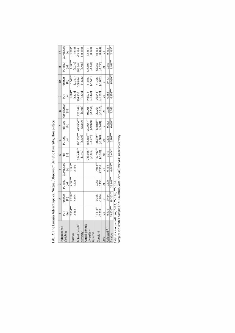
Tab.

7: T

he E

uras

ia A

dvan

tage

vs.

“Act

ual/O

bser

ved”

Gen

etic

Div

ersit

y, H

orse

-Rac

e

Inde

pend

ent

Varia

bles

1 2

3 4

5 6

7 8

9 10

11

12

PD

1 (ln

) PD

1000

(ln

) PD

1500

(ln

) GD

Ppc2

000

(ln)

PD1

(ln)

PD10

00

(ln)

PD15

00

(ln)

GDPp

c200

0(ln

) PD

1 (ln

) PD

1000

(ln

) PD

1500

(ln

) GD

Ppc2

000

(ln)

Eura

sia

2. 3.35

4***

952

2. 4.23

8***

044

2. 4.56

8***

821

1. 2.14

1**

156

1. (2.68

4**

331)

1. (2.57

2**

367)

1. (3.96

6***

077)

1. (1.26

3*

918)

Ac

tual

gen

etic

di

vers

ity

394. (3.44

8***

107)

39

0. (3.93

5***

327)

41

3. (3.50

4***

382)

12

3. (1.14

6 10

5)

204. (1.82

0 47

0)

208. (1.84

4 60

6)

185. (1.84

4 48

6)

-23.

(-0.

164

180)

Ac

tual

gen

etic

di

vers

ity -

squa

red

-289

.(-

3.05

6***

054)

-2

86.

(-3.

582*

**27

5)

-302

.(-

3.64

7***

323)

-9

6.(-

1.00

8 15

6)

-149

.(-

1.03

4 44

0)

-151

.(-

1.84

6 57

1)

-134

.(-

1.19

3 44

4)

12.

(0.25

1 12

8)

Cons

tant

-1

.-2

.118*

*79

8 -0

.-1

.396

094

0. 0.06

8 19

6 7. 22.95

3***

956

-133

.(-

3.49

2***

161)

-1

31.

(-3.

619*

**36

5)

-138

.(-

3.88

9***

411)

-3

0.(-

0.26

1 81

5)

-70.

(-1.

643

526)

-7

1.(-

1.36

5 65

2)

-63.

(-1.

556

530)

18

.(0

.153

424)

O

bs.

20

21

21

21

20

21

21

21

20

21

21

21

Adju

sted

R2

0.43

5 0.

434

0.52

7 0.

154

0.31

7 0.

338

0.35

2 0.

026

0.45

8 0.

473

0.55

9 0.

152

F va

lue

15.6

20**

*16

.353

***

23.2

42**

*4.

649*

*5.

404*

* 6.

107*

**6.

438*

**1.

265

6.35

3***

6.98

0***

9.46

7***

2.19

5*

t st

atist

ics

in p

aren

thes

is; *<

0.1;

**<0

.05;

***<

0.01

. Sa

mpl

e: T

he L

imite

d Sa

mpl

e of

21

Coun

trie

s, w

ith “

Actu

al/O

bser

ved”

Gen

etic

Div

ersit

y

Tab.

8A:

G

enet

ic D

iver

sity,

Anc

estr

y Ad

just

ed o

r not

, Ind

epen

dent

ly T

este

d (E

uras

ia o

nly)

Inde

pend

ent

Varia

bles

1 2

3 4

5 6

7 8

PD1

(ln)

PD10

00

(ln)

PD15

00

(ln)

GDP

pc20

00

(ln)

PD1

(ln)

PD10

00

(ln)

PD15

00

(ln)

GDP

pc20

00

(ln)

Pred

icte

d G

enet

ic

Dive

rsity

-2

07.

(-0.

674

308)

15

2. (0.20

1 24

7)

208. (0.73

5 32

0)

73.

(0.73

3 14

3)

Pred

icte

d G

enet

ic

Dive

rsity

-squ

ared

16

0. (0.24

1 34

1)

-101

.(-

0.45

1 23

6)

-145

.(-

0.98

8 32

1)

-47.

(-0.

263

132)

Pred

icte

d G

enet

ic D

iver

sity

-anc

estr

y ad

just

ed

-366

.(-

0.25

9 49

6)

170. (0.74

7 25

6)

351. (0.10

0 50

3)

546. (0.34

7 94

3)

Pred

icte

d G

enet

ic D

iver

sity

-anc

estr

y ad

just

ed -

squa

red

270. (0.36

0 52

6)

-115

.(-

0.71

1 24

9)

-247

.(-

0.09

2 50

8)

-372

.(-

0.66

0 92

2)

Cons

tant

66

.(0

.947

27

7 )

-55.

(-0.

848

253)

-7

2.(-

0.89

0 31

2)

-19.

(-0.

639

107)

12

4. (0.00

3 46

8)

-61.

(-0.

767

259)

-1

22.

(-0.

890

491)

-1

91.

(0.19

0 36

0)

Obs

erva

tions

72

80

81

85

72

79

80

81

Ad

just

ed R

2 0.

066

-0.0

15

-0.0

24

-0.0

13

0.05

8 -0

.021

-0

.020

0.

021

F va

lue

3.49

4**

0.40

3 0.

055

0.45

2 3.

186*

* 0.

210

0.21

1 1.

863

t st

atist

ics

in p

aren

thes

is; *<

0.1;

**<0

.05;

***<

0.01

.

Tab.

8B:

G

enet

ic D

iver

sity,

Anc

estr

y Ad

just

ed o

r not

, Ind

epen

dent

ly T

este

d (E

uras

ia o

nly)

Inde

pend

ent

Varia

bles

1 2

3 4

5 6

7 8

PD1

(ln)

PD10

00

(ln)

PD15

00

(ln)

GDP

pc20

00

(ln)

PD1

(ln)

PD10

00

(ln)

PD15

00

(ln)

GDP

pc20

00

(ln)

Pred

icte

d G

enet

ic

Dive

rsity

(ln)

X

X X

X

Pred

icte

d G

enet

ic

Dive

rsity

-squ

ared

(ln)

35

.(2

.444*

**

639)

10

.(0

.587

870)

-1

.(-

0.09

0 08

4)

9. (0.53

2 94

6)

Pred

icte

d G

enet

ic D

iver

sity

-anc

estr

y ad

just

ed (l

n)

X X

X X

Pred

icte

d G

enet

ic D

iver

sity

-anc

estr

y ad

just

ed (l

n)-

squa

red

34.

(2.75

2**

484)

7. (0.51

2 60

1)

-5.

(-0.

415

411)

18

.(1

.522*

69

4)

Cons

tant

-9

.(2

.869*

* 45

8 )

-2.

(-0.

014

553)

1. (0.97

7 51

1)

6. (2.12

3**

037)

-9

.(-

2.66

6**

310)

-1

.(-

0.07

2 28

7)

3. (0.29

9 83

5)

3. (1.39

0 03

6)

Obs

erva

tions

72

79

80

81

72

79

80

81

Ad

just

ed R

2 0.

078

-0.0

03

-0.0

13

-0.0

01

0.06

8 -0

.008

-0

.011

0.

023

F va

lue

6.96

7***

0.

758

0.00

7 0.

896

6.17

1**

0.36

1 0.

169

2.86

8*

t st

atist

ics

in p

aren

thes

is; *<

0.1;

**<0

.05;

***<

0.01

. N

ote:

“X”

mea

ns t

hat

the

first

ord

er t

erm

of

pred

icte

d ge

netic

div

ersit

y (ln

), w

heth

er a

nces

try

adju

sted

or n

ot, i

s co

nsist

ently

elim

inat

ed a

utom

atic

ally

dur

ing

regr

essio

n du

e to

str

ong

colli

near

ity, i

ndic

atin

g th

at t

he f

irst

orde

r te

rm a

nd t

he s

econ

d or

der

term

hav

e no

diff

eren

t im

pact

ove

r in

dica

tors

of

econ

omic

de

velo

pmen

t.

Tab.

9: B

oth

Geo

com

pone

nts

and

Bioc

ompo

men

ts a

re L

arge

ly D

eter

min

ed b

y Eu

rasia

(Ful

l Sam

ple:

The

Who

le W

orld

)

Inde

pend

ent

Varia

bles

1 2

3 4

5 6

7 8

9 10

G

eoco

m1

(O&

H)

Geo

com

2 (P

&S)

G

eoco

m3

(P&

S)

Bioc

om1

(O&

H)

Bioc

om2

(P&

S)

Geo

com

1 (O

&H

) G

eoco

m2

(P&

S)

Geo

com

3 (P

&S)

Bi

ocom

1 (O

&H

) Bi

ocom

2 (P

&S)

Eura

sia

1.(1

3.67

0***

962)

1.

(18.

630*

**51

7)

1.(1

3.43

8***

516)

1.

(13.

532*

**29

3)

1.(1

7.60

9***

666)

Land

lock

ed

-0

.(-

1.26

8 58

5)

-0.

(-0.

083

637)

-0

.(-

1.14

2 11

1)

-0.

(-1.

249

338)

-0

.(-

1.23

5 58

3)

Abso

lute

la

titud

e (ln

)

0.(1

0.71

3***

151)

0.

(12.

660*

**24

3)

0.(1

3.72

7***

802)

0. (7.58

2***

647)

0. (9.61

1***

943)

Isla

nd

-0

.(-

3.64

7***

714)

-0

.(-

4.67

7***

984)

-0

.(-

2.39

0***

937)

-0

.(-

1.21

0 11

3)

-0.

-2.41

4***

681

Cons

tant

-0

.(-

8.68

4***

735)

-0

.(-

12.79

1***

815)

-0

.(-

9.70

1***

397)

-0

.(-

9.70

1***

196)

-0

.(-

12.79

0***

338)

-1

.(-

8.80

2***

105)

-1

.(-

10.76

1***

098)

-2

.(-

11.00

9***

778)

-1

.(-

6.60

0***

615)

-1

.(-

8.64

8***

253)

O

bser

vatio

ns

112

171

171

112

170

112

171

171

112

170

Adju

sted

R2

0.63

6 0.

668

0.51

7 0.

613

0.64

8 0.

514

0.53

0 0.

552

0.34

6 0.

398

F va

lue

94.9

24**

*34

2.88

0***

182.

673*

**17

6.69

3***

312.

078*

**40

.168

***

64.8

12**

*70

.739

***

20.5

76**

*38

.238

***

Not

e: O

&H

is O

lsson

and

Hib

bs (2

005)

whe

reas

P&

S is

Pete

rsen

and

Ska

anin

g (2

010)

t s

tatis

tics

in p

aren

thes

is; *<

0.1;

**<0

.05;

***<

0.01

.

Tab.

9 (c

ontin

ued)

: Bot

h G

eoco

mpo

nent

s an

d Bi

ocom

pom

ents

are

Lar

gely

Det

erm

ined

by

Eura

sia (F

ull S

ampl

e: T

he W

hole

Wor

ld)

Inde

pend

ent

Varia

bles

11

12

13

14

15

Geo

com

1 (O

&H

) G

eoco

m2

(P&

S)

Geo

com

3 (P

&S)

Bi

ocom

1 (O

&H

) Bi

ocom

2 (P

&S)

Eura

sia

1.(1

5.39

0***

63

2)

1.(1

6.26

8***

96

8)

0. (9.92

9***

57

2)

1.(1

0.31

4***

93

5)

1.(1

4.33

3***

14

0)

Land

lock

ed

-0.

(-1.

176*

87

5)

-0.

(-1.

095

199)

-0

.(-

1.15

1 46

4)

-0.

(-1.

164

276)

-0

.(-

2.24

6**

454)

Ab

solu

te

latit

ude

(ln)

0. (8.36

7***

18

6)

0. (8.31

9***

32

1)

0. (9.47

8***

60

0)

0. (4.25

2***

15

5)

0. (5.25

5***

25

1)

Isla

nd

-0.

(-8.

853*

**

753)

-0

.(-

8.69

0***

37

0)

-0.

(-3.

399*

**

735)

-0

.(-

3.39

9***

03

7)

-0.

(-4.

425*

**

081)

Cons

tant

-1

.(-

10.38

7***

99

7)

-1.

(-12

.384*

**

797)

-1

.(-

12.73

2***

34

4)

-1.

(-7.

206*

**

059)

-1

.(-

9.25

7***

14

7)

Obs

erva

tions

11

2 17

1 17

1 11

2 17

0 Ad

just

ed R

2 0.

851

0.82

7 0.

709

0.68

8 0.

726

F va

lue

159.

095*

**

204.

094*

**

104.

746*

**

62.2

65**

* 11

3.03

4***

N

ote:

O&

H is

Olss

on a

nd H

ibbs

(200

5) w

here

as P

&S

is Pe

ters

en a

nd S

kaan

ing

(201

0)

t sta

tistic

s in

par

enth

esis;

*<0.

1; **

<0.0

5; **

*<0.

01.

Tab.

10:

Det

erm

inan

ts o

f G

eoco

mpo

nent

s an

d Bi

ocom

pom

ents

with

in E

uras

ia (S

ampl

e: E

uras

ia)

Inde

pend

ent

Varia

bles

1 2

3 4

5 G

eoco

m1

(O&

H)

Geo

com

t2

(P&

S)

Geo

com

3 (P

&S)

Bi

ocom

1 (O

&H

) Bi

ocom

2 (P

&S)

Land

lock

ed

-0.

(-0.

029

160)

-0

.(-

0.07

1 56

8)

-0.

(-1.

205

436)

-0

.(-

0.10

2 41

8)

-0.

(-2.

327*

* 29

6)

Abso

lute

la

titud

e (ln

) 0. (5.48

9***

72

6)

0. (6.47

3***

11

3)

0. (9.82

4***

34

4)

0. (3.35

9***

11

3)

0. (4.42

7***

87

2)

Isla

nd

-0.

(-5.

964*

**

690)

-0

.(-

5.82

3***

51

8)

-0.

(-1.

338*

* 98

7)

-0.

(-1.

399*

89

7)

-0.

(-2.

472*

**

792)

Cons

tant

-0

.(-

1.40

9 28

9)

-0.

(-2.

627*

* 23

0)

-1.

(-6.

994*

**

222)

-0

.(-

0.43

5 60

2)

-0.

(-1.

493

545)

O

bser

vatio

ns

48

84

84

49

84

Adju

sted

R2

0.69

1 0.

570

0.59

1 0.

269

0.35

3 F

valu

e 36

.041

***

37.7

09**

* 40

.990

***

6.89

7***

16

.108

***

Not

e: O

&H

is O

lsson

and

Hib

bs (2

005)

whe

reas

P&

S is

Pete

rsen

and

Ska

anin

g (2

010)

t

stat

istic

s in

par

enth

esis;

*<0.

1; **

<0.0

5; **

*<0.

01.

Tab:

11:

Th

e Eu

rasia

Adv

anta

ge T

hesis

Vin

dica

ted:

The

Eur

asia

Adv

anta

ge p

lus

Diff

usio

n (F

ull S

ampl

e: t

he W

hole

Wor

ld)

Inde

pend

ent

Varia

bles

1 2

3 4

5 6

7 8

PD1

(ln)

PD10

00

(ln)

PD15

00

(ln)

GDP

pc20

00

(ln)

PD1

(ln)

PD10

00

(ln)

PD15

00

(ln)

GDP

pc20

00

(ln)

Eura

sia

1. (8.65

2***

54

3)

1. (7.28

1***

00

7)

1. (7.37

2***

38

0)

0. (5.81

4***

00

3)

Dist

ance

to

Fron

tier

AD1

-0

.(-

7.59

5***

55

3)

Dist

ance

to

Fron

tier

AD10

00

-0.

(-4.

387*

**

644)

Dist

ance

to

Fron

tier

AD15

00

-0.

(-5.

351*

**

059)

-0

.(-

3.18

6***

24

9)

Cons

tant

-0

.(-

7.93

1***

06

2)

-0.

(-1.

130

055)

0. (2.27

9**

263)

8.

(74.

151*

**

342)

4. (7.25

5***

17

0)

3. (5.35

6***

29

9)

3. (6.40

4***

70

2)

9.(2

2.91

1***

72

5)

Obs

erva

tions

15

5 17

7 18

4 18

7 15

5 17

7 18

4 18

7 Ad

just

ed R

2 0.

319

0.21

5 0.

226

0.11

4 0.

267

0.10

5 0.

118

0.04

9 F

valu

e 72

.982

***

49.0

97**

* 54

.462

***

25.0

31**

* 57

.047

***

21.5

70**

* 25

.591

***

10.5

57**

* t

stat

istic

s in

par

enth

esis;

*<0.

1; **

<0.0

5; **

*<0.

01.

Tab:

11

(con

tinue

d): T

he E

uras

ia A

dvan

tage

The

sis V

indi

cate

d: T

he E

uras

ia a

dvan

tage

plu

s Di

ffus

ion

(Ful

l Sam

ple:

the

Who

le W

orld

)

Inde

pend

ent

Varia

bles

9 10

11

12

13

14

15

16

PD

1 (ln

) PD

1000

(ln

) PD

1500

(ln

) G

DPpc

2000

(ln

) PD

1 (ln

) PD

1000

(ln

) PD

1500

(ln

) G

DPpc

2000

(ln

)

Eura

sia

1. (6.27

5***

75

3)

1. (5.10

1***

77

9)

1. (6.17

3***

15

5)

0. (4.71

4***

21

9)

1. (6.42

2***

46

8)

1. (6.42

5***

58

9)

1. (7.56

8***

22

9)

0. (2.48

6***

95

0)

Dist

ance

to

Fron

tier

AD1

(ln)

-0.

(-5.

417*

**

628)

-0.

(-5.

422*

**

345)

Dist

ance

to

Fron

tier

AD10

00 (l

n)

-0

.(-

2.22

9***

81

4)

-0

.(-

3.27

9***

25

9)

Dist

ance

to

Fron

tier

AD15

00 (l

n)

-0.

(-3.

214*

**

340)

-0

.(-

1.11

3**

973)

-0

.(-

4.27

5***

18

8)

-0.

(-1.

078

498)

Land

lock

ed

-0.

(-1.

433*

86

9)

-0.

(-1.

262

148)

0. (0.02

7 11

7)

-0.

(-3.

640*

**

531)

Ab

solu

te L

atitu

de

(ln)

-0.

(-0.

062

522)

-0

.(-

2.30

5***

65

4)

-0.

(-3.

376*

**

279)

0. (4.40

9***

74

0)

Isla

nd

0. (0.09

8 41

9)

0. (0.19

4 85

6)

0. (1.35

0 59

7)

0. (4.79

6***

69

6)

Cons

tant

2. (3.34

3***

94

4)

1. (2.67

0**

566)

1. (3.96

5***

78

7)

9.(1

9.04

4***

43

1)

2. (3.55

8***

51

5)

2. (3.80

5***

63

6)

3. (5.25

0***

08

3)

7.(1

5.62

4***

09

7)

Obs

erva

tions

15

5 17

7 18

4 18

7 15

5 17

7 18

4 18

7 Ad

just

ed R

2 0.

432

0.24

4 0.

267

0.12

8 0.

439

0.27

4 0.

304

0.35

9 F

valu

e 59

.641

***

29.4

78**

* 34

.328

***

14.6

59**

* 25

.086

***

14.2

72**

* 17

.006

***

21.8

13**

* t s

tatis

tics

in p

aren

thes

is; *<

0.1;

**<0

.05;

***<

0.01

.

The Journal: Cooperations, Archiving & Coverage

HSR 41 (2016) 1 │ 360

Cooperating Associations / Networks / Journals

QUANTUM (Association for Quantification and Methods in Historical and Social Re-search) http://www.gesis.org/en/hsr/profile/quantum.

INTERQUANT (International Commission of the application of Quantitative Methods in History) http://www.gesis.org/en/hsr/profile/quantum.

H-SOZ-KULT (Communication and Information Services for Historians) http://www. hsozkult.de.

AFC (Association Française de Cliométrie) http://www.cliometrie.org. AGE (Arbeitsgemeinschaft Geschichte und EDV) http://www.age-net.de. AHC (International Association for History and Computing) http://odur.let.rug.nl/ahc. FQS (Forum Qualitative Sozialforschung – Forum Qualitative Social Research) http://

www.qualitative-research.net/fqs. HISTORICUM.NET http://www.historicum.net.

ZOL (Zeitgeschichte-online) http://www.zeitgeschichte-online.de. PERSPECTIVIA.NET http://www.perspectivia.net.

Archiving by Information Services

JSTOR (ITHAKA) http://www.jstor.org/r/histsocres. SSOAR (Social Science Open Access Repository) http://www.ssoar.info.

Coverage by Information Services

In recognition of the high quality and relevance to the scientific community our journal Historical Social Research has been selected for coverage / archiving in the following databases:

Social Science Citation Index (Thomson Scientific) http://scientific.thomson.com/ products/ssci.

SCOPUS (Elsevier) http://www.scopus.com.

SocINDEX with FULL TEXT (EBSCO) https://www.ebscohost.com. Sociological Abstracts (ProQuest) http://www.csa.com.

Historical Abstracts (ABC-CLIO) https://www.ebscohost.com/academic/historical-abstracts.

International Political Science Abstracts (SAGE) http://www.sagepub.co.uk.

SOLIS (Social Science Literature Information System / GESIS) http://www.gesis.org/en/ services/research/solis-social-science-literature-information-system.