Historical Costs of Coal-Fired Electricity and Implications for the Future

James McNerney∗,a,b, Jessika E. Trancik∗,b,d, J. Doyne Farmerb,c

aDepartment of Physics, Boston University, Boston, MA 02215, USAbSanta Fe Institute, 1399 Hyde Park Road, Santa Fe, NM 87501, USA

cLUISS Guido Carli, Viale Pola 12, 00198, Roma, ItalydEngineering Systems Division, Massachusetts Institute of Technology, Cambridge, MA 02139-4307, USA

Abstract

We study the costs of coal-fired electricity in the United States between 1882 and 2006 by decomposing it in terms of theprice of coal, transportation costs, energy density, thermal efficiency, plant construction cost, interest rate, and capacityfactor. The dominant determinants of costs at present are the price of coal and plant construction cost. The price ofcoal appears to fluctuate more or less randomly while the construction cost follows long-term trends, decreasing from1902 - 1970, increasing from 1970 - 1990, and leveling off or decreasing a little since then. This leads us to forecast thateven without carbon capture and storage, and even under an optimistic scenario in which construction costs resumetheir previously decreasing trending behavior, the cost of coal-based electricity will drop for a while but eventually bedetermined by the price of coal, which varies stochastically but shows no long term decreasing trends. Our analysisemphasizes the importance of using long time series and comparing different electricity generation technologies usingtotal costs, rather than costs of single components like capital.

Contents

1 Introduction 1

2 Historical data 22.1 Data sources . . . . . . . . . . . . . . . . . 22.2 Decomposition formula . . . . . . . . . . . . 22.3 Fuel cost . . . . . . . . . . . . . . . . . . . 3

2.3.1 Coal price . . . . . . . . . . . . . . . 32.3.2 Transportation costs . . . . . . . . . 32.3.3 Coal energy density . . . . . . . . . 32.3.4 Thermal efficiency . . . . . . . . . . 42.3.5 Fuel cost . . . . . . . . . . . . . . . 5

2.4 Operation and maintenance cost . . . . . . 52.5 Capital cost . . . . . . . . . . . . . . . . . 5

2.5.1 Specific construction cost . . . . . . 52.5.2 Capacity factor . . . . . . . . . . . . 62.5.3 Interest rate . . . . . . . . . . . . . . 62.5.4 Capital cost . . . . . . . . . . . . . . 7

2.6 Total cost . . . . . . . . . . . . . . . . . . . 7

3 Analysis of cost trends 8

4 Analysis of cost variation 9

5 Extrapolation 105.1 Commodities vs. pure technologies . . . . . 115.2 Modeling a commodity . . . . . . . . . . . . 115.3 Modeling a technology . . . . . . . . . . . . 12

∗Corresponding author

5.4 Capital and O&M costs . . . . . . . . . . . 125.5 Fuel costs . . . . . . . . . . . . . . . . . . . 135.6 Extrapolation summary . . . . . . . . . . . 145.7 Extrapolation results . . . . . . . . . . . . . 14

6 Conclusions 14

7 Acknowledgments 15

A Change decomposition 15

1. Introduction

Coal generates two-fifths of the world’s electricity [1]and almost a quarter of its carbon dioxide emissions [2].The impact of any market-based effort to reduce carbonemissions will be highly sensitive to future costs of coal-fired electricity in comparison to other energy technolo-gies. The relative cost of technologies will, for example,determine the carbon reductions resulting from a partic-ular carbon tax or the cost of a given cap on emissions.However, no study exists that examines total generationcosts and component contribitions using data over a timespan comparable to that of the forecasts needed. Thisstudy attempts to fulfill this need. We also aim to makemethodological advances in the analysis of historical en-ergy costs and implications for future costs.

To do this, we build a physically-accurate model ofthe total generation cost in terms of the price of coal,coal transportation cost, coal energy density, thermal effi-ciency, plant construction cost, the interest rate, and thecapacity factor. This contrasts with the approach taken in

Preprint submitted to Elsevier January 5, 2010

arX

iv:1

001.

0605

v1 [

phys

ics.

soc-

ph]

5 J

an 2

010

econometrics, where generation costs, or more typicallyplant costs, are broken down using a regression model[3, 4, 5, 6, 7, 8, 9, 10, 11, 12, 13].

We also focus on the long term evolution of quanti-ties averaged across plants in the United States, goingback to the earliest coal-fired power plant in 1882 through2006, rather than cross-sections or panels of plants. Thus,our data set sacrifices cross-sectional richness to examinea longer time span (over a century). This is important forcharacterizing the factors driving the long term evolutionof costs.

The data suggests a qualitative difference between thebehavior of fuel and capital costs, the two most significantcontributors to total cost. Coal prices, which became themost important determinants of fuel costs when averagethermal efficiencies ceased improving in the U.S. duringthe 1960s, have fluctuated and shown no overall trend upor down. This fluctuation and lack of trend are consis-tent with the facts that coal is a traded commodity andtherefore it should not be possible to make easy arbitrageprofits by trading it. According to standard results in thetheory of finance, this implies that it should follow a ran-dom walk. In contrast, plant construction costs, the mostimportant determinant of capital costs, followed a decreas-ing trajectory until 1970, consistent with what one expectsfrom a technology. This pattern continued until 1970 whenconstruction costs dramatically reversed direction, at leastin part due to pollution controls.

To probe the future of coal-fired electricity, we study itscosts in a reasonable best case scenario. We study a low-cost scenario for future generation costs involving a returnof plant cost improvement to its pre-1970 rate. Undersuch a scenario, we estimate that capital costs would drop67% over 50 years, reducing total generation costs by 40%.At the same time, fuel costs would rise in their relativecontribution to the total, leading to higher uncertainty intotal generation costs, and creating a floor below whichthe generation cost would be unlikely to drop.

Our analysis makes several methodological advances.It calculates total costs of generation, rather than thecosts of individual components like capital, and over a long(∼100 year) time span. We repeat and refine an approachused by Nemet [14] to decompose changes in cost. Therefinement eliminates artificial residuals arising from thecross-effects of variables influencing the cost. Finally, wenote that physically accurate models like the one presentedhere and in Nemet may sometimes allow (data permitting)for more reliable decompositions of cost than regressionmodels.

The paper is organized as follows: in Section 2, wepresent the historical record of costs for coal-fired electric-ity, as represented by time series for a number of importantvariables influencing generation cost. The generation costconsists of three main components – fuel, capital, and op-eration and maintenance. The first two are further decom-posed; the fuel component into the coal price, transporta-tion cost, coal energy density, and thermal efficiency; the

capital component into plant construction costs, capacityfactor, and interest rate. In Section 3, we determine thevariables contributing most to the historical changes ingeneration costs, focusing on their long term trends ratherthan their short term variation. In Section 4, we examinethe effect their short term variation has on the variation oftotal generation costs. In Section 5, we use the experiencegained from analyzing the data to construct two possibleextrapolations of coal-fired generation costs.

2. Historical data

2.1. Data sources

Sources for data are given in the captions of the rele-vant figures. The data comes from the U.S. Energy Infor-mation Administration, Census Bureau, Bureau of Mines,Federal Energy Regulatory Commission (formerly the Fed-eral Power Commission), Federal Reserve, the Edison Elec-tric Institute, and the Platts UDI world electric powerplants database, with some minor contributions from a fewother databases and technical reports. Methods for han-dling specific data issues are described in the Appendixand in the Supporting Information. Assumptions made tofill in for missing data are noted in the relevant figures andtext.

All data presented here are for the United States be-tween 1882 (the approximate beginning of the electricityutility industry in the U.S.) and 2006. All data are esti-mates for averages over U.S. coal utility plants. All pricesand costs are presented in real 2006 currency, deflatedusing the GDP deflator. The data is made available atwww.santafe.edu/files/coal electricity data.

2.2. Decomposition formula

We seek to build up the total generation costs from thefollowing variables, for which data is available:

OM = operation and maintenance cost (¢/kWh)

COAL = price of coal ($/ton)

TRANS = price of transporting coal to plant ($/ton)

ρ = energy density of coal (Btu/lb)

η = plant efficiency

SC = specific construction cost ($/kW)

r = nominal interest rate

CF = capacity factor

Specific construction cost (SC) here means the construc-tion cost of a plant per kilowatt of capacity. Each variableis given a subscript t to denote its value in year t. Thetotal generation cost (TC) in year t is

TCt = OMt + FUELt + CAPt (1)

= OMt +COALt + TRANSt

ρtηt+

SCt × CRF(rt, n)

CFt × 8760 hrs/year.

2

The three main terms are the three major cost components– operation and maintenance, fuel, and capital. The fuelcomponent accounts for the cost of coal and its deliveryto the plant, the amount of energy contained in coal, andthe efficiency of the plant in converting stored chemicalenergy to electricity. The capital component levelizes theconstruction cost of the plant using the capital recoveryfactor, CRF(rt, n), defined as

CRF(rt, n) =rt(1 + rt)

n

(1 + rt)n − 1, (2)

where n is the plant lifetime in years. The capital recov-ery factor is the fraction of a loan that must be payedback annually, assuming a stream of equal payments overn years and an annual interest rate rt. For a plant of ca-pacity K, the capital component is the annuity paymenton money borrowed for construction, K×SCt×CRF(rt, n),divided by the yearly electricity production of the plant,K×CFt×8760 hrs/year. Note that K cancels out. Thus,the capital component is the annuity payment on borrowedplant construction funds per kilowatt-hour of annual elec-tricity production by the plant. We follow convention andlevelize over an assumed plant lifetime of n = 30 years.

Note that the total cost for year t uses the capital costof plants built that year, while the actual fleet of plantsexisting in year t also includes plants built in previousyears. Since we do not have data on the retirement datesof plants, we use the cost of the plants built in year t toestimate the cost of electricity generated in that year. Av-erage capital costs of the whole fleet existing in a particularyear would have the same basic evolution as that of newplants alone, but tend to lag the latter, since they wouldinclude capital costs from previous years.

In Sections 2.3 – 2.5, we present and discuss the time-series data for each of these variables separately. In Section2.6 we combine the variables to compute the total cost,and examine the effect that individual variables had onit. The ensuing sections are an extensive discussion of thedata; readers more interested in final analyses may wishto skip to Section 3.

2.3. Fuel cost

2.3.1. Coal price

Real coal prices (COAL) have varied over the past 130years (Fig. 1.) The largest change occurred between 1973and 1974. A government study [15] found this was due tothe OPEC oil embargo started in December 1973, whichraised prices for substitutes coal and natural gas, and an-ticipation of a strike by the United Mine Workers union,which later occurred at the end of 1974. Wage increasesstarting in 1970 also played a somewhat less importantrole.

Coal prices at the mine were derived from price time-series for individual varieties of coal. For the period 1882-1956, the coal price is a production-weighted average overanthracite and bituminous varieties, and for 1957-2006

1880 1900 1920 1940 1960 1980 2000

101

102

Cost

& P

rice

(200

6 $/

ton)

Mining and transport cost of coal

Delivered cost of coal (COAL+TRANS)Price of coal (COAL)Transportation price (TRANS)

Figure 1: The price of coal at the mine, the price of transporting itto the plant, and their sum. The price of coal has fluctuated withno clear trend up or down. Transportation contributed a significantwhile decreasing expense to fuel costs. Source: [16, 17, 18, 19, 20]

over anthracite, bituminous, subbituminous, and lignite.No data could be found to weight prices by the quanti-ties in which they were consumed by plants, and thereforewe relied on the quantities in which they were produced.The resulting average price series closely resembles that ofbituminous coal by itself.

2.3.2. Transportation costs

Transportation costs (TRANS) were derived mainlyfrom the cost of coal delivered to power plants and theprice of coal at the mine, though some direct data also ex-ists. Transportation costs have added a significant thoughdecreasing amount to the cost of coal delivered to powerplants (Fig. 1). Transportation costs before 1940 were onpar with the price of coal at the mine; since 1940, theyhave dropped to 20 – 40% of the delivered cost on aver-age, though there is considerable variation from plant toplant. The introduction of unit trains in the 1950s mayaccount for some of the decrease in transportation costs.A unit train carries a single commodity from one origin toone destination, shortening travel times and eliminatingthe confusion of separating cars headed for different desti-nations. About 50% of coal shipped in the United States(90% of which is used by utilities) is carried by unit trains[21]. Other means of transporting coal are barges, collierships, trucks, and conveyor belts in cases where plants arebuilt next to mines.

Many utilities responded to environmental regulationsby switching to higher priced, low-sulfur coals [10]. Switch-ing to low sulfur coals also extended transportation dis-tances, which may explain the increase in transportationcosts seen around 1970.

2.3.3. Coal energy density

Since 1960, the average energy density of coal (ρ) hasdropped steadily (Fig. 2 inset.) The lower the energydensity, the more coal needed by plants to consume equalamounts of primary energy. Thus, the effect of lower en-

3

1880 1900 1920 1940 1960 1980 2000

0.5

1

2

3

Cos

t of e

nerg

y (2

006

cent

s/kW

h)

1880 1900 1920 1940 1960 1980 20001

2

5

10

Cos

t of e

nerg

y (2

006

$/M

MB

tu)

Energy density and cost of energy

1880 1900 1920 1940 1960 1980 20000

2,0004,0006,0008,000

10,00012,00014,000

ρ (B

tu/lb

)

Energy density of coal ρ

Figure 2: The cost of coal-stored energy, (COALt + TRANSt)/ρt.The left axes show cost in dollars per million BTU, the right axes incents per kWh. The inset shows the energy density of coal in Btuper pound. The dashed line indicates an assumed value of 12,000Btu per pound. Coal energy densities have come down about 16%in the last 40 years. Source: [22, 17]

ergy densities has been to increase fuel costs through in-creased purchase and transportation costs.

Changes in the energy density reflect changes in theoverall mixture of coal species used by the industry, as wellas variation of energy density within species. One cause ofthe decrease in energy density may be the increased use ofsubbituminous coal, which burns more cleanly than previ-ously used bituminous due to a lower sulfur content, butalso contains less energy per pound. No data for energydensity could be found before 1938, and a value of 12,000Btu per pound was assumed (the 1938 value).

2.3.4. Thermal efficiency

The thermal efficiency of a fossil-steam plant (η) is thefraction of stored chemical energy in fuel that is convertedinto electrical energy (Fig. 3). It accounts for every effectwhich causes energy losses between the input of fuel andthe bus-bar of the plant, the point where electricity entersthe electric grid. These effects include incomplete burn-ing of fuel, radiation and conduction losses, stack losses,excess entropy produced in the turbine, friction and windresistance in the turbine, electrical resistance, power torun the boiler feed pump and other plant equipment, andthe thermodynamic limits of the heat cycle used.

Over the first 80 years, the average efficiency of coalplants increased by more than a factor of 10. The earliestplants obtained efficiencies below 3%. Improving efficien-cies meant that less coal was required to produce equalamounts of electricity, lowering fuel costs. For the last 50years, the average efficiency of coal-fired plants has stayedapproximately level at 32–34%, although individual plantsobtained efficiencies as high as 40% during the 1960s [23].

The factors influencing efficiency of plants fall into twomajor categories: thermodynamic factors, which pertainto the specific heat cycle employed, and operational fac-tors, which reflect the mechanical and electrical efficiencies

1880 1900 1920 1940 1960 1980 20000

0.2

0.4

0.6

0.8

1

Effi

cien

cy η

1880 1900 1920 1940 1960 1980 200010

−1

100

101

102

FU

EL

(200

6 ce

nts/

kWh)

Efficiency and fuel cost

Fuel Cost (FUEL)Efficiency (η)

Figure 3: Average efficiency of coal plants and cost of the fuel com-ponent, (COALt + TRANSt)/(ρtηt). Efficiency increases drove de-creases in fuel costs until 1960. Since then efficiency has remainedstable around 32 – 34%. Source: [24, 17]

of individual stages and components. The thermodynamiclimit efficiency is determined by the details of the steamcycle used – the maximum and minimum temperatures,the maximum and minimum pressures, and the exact typeof cycle followed (e.g. the number of reheat stages used.)Current plant designs typically have thermodynamic limitefficiencies around 46%.1 The operational efficiencies ofthe boiler, turbine, generator, and other components fur-ther reduce the efficiency achievable in practice (Table 1.)The net effect of the operational efficiencies is to reducetotal efficiency by a factor of about 0.7.

Historical increases in efficiency came from improve-ments in both the thermodynamic and operational cat-egories. Higher steam temperatures, higher steam pres-sures, and changes to the heat cycle relaxed the thermo-dynamic constraint, while better designed parts reducedoperational losses. However, operational factors are nowworking at high efficiencies (Table 1), while changing theparameters of the heat cycle faces highly diminishing re-turns for efficiency [23]. This latter problem reduces incen-tives to develop economical materials that could withstandhigher pressures and temperatures. The overall result hasbeen a standstill in average efficiency for the last 50 years.Given the present technological options, the current aver-

1We assume a Rankine cycle with superheating and one reheatcycle operating at 1000 ◦F, 2400 psi.

Table 1: Operational sources of energy loss. Source: [23]

Source of energy loss EfficiencyStack losses, radiation

& conduction from boiler 87%Excess entropy produced in turbine 92%Windage, friction, & elec. resistance 95%Boiler feed pump power requirement 95%Auxiliary power requirements 97%Total (product) 70%

4

1880 1900 1920 1940 1960 1980 200010

−1

100

101

102

OM

(20

06 c

ents

/kW

h)

Operation and maintenance cost

.21 x FUELt

Figure 4: The cost of operation and maintenance of coal plants. Avalue equal to 21% of the overall fuel cost for a given year was usedto fill in missing data. Source: [22, 25, 26, 27, 28, 29]

age efficiency presumably represents an optimum after bal-ancing the higher fuel cost of a less efficient plant againstthe higher construction costs of a more efficient plant.

2.3.5. Fuel cost

Over the entire time period (1882-2006) the factorsmost responsible for changes in the fuel cost are the priceof coal and the efficiency. Changes in energy density andtransportation costs had relatively minor effects. As canbe seen in Fig. 3, the net effect of varying coal price, en-ergy density, transportation cost, and efficiency on the fuelcomponent of electricity costs was a long term decrease inthe cost of the fuel component until about 1970. The de-crease was mainly due to improving efficiency. After 1970,coal prices increased dramatically during a time when ef-ficiency was flat, increasing overall fuel costs 70% between1970 and 1974.

2.4. Operation and maintenance cost

The O&M cost (OM) is the least significant of the threecost components (fuel, O&M, capital), representing about5-15% of total generation costs during the last century(Fig. 11). Although it is less significant than fuel or cap-ital, we attempted to reconstruct a time-series for O&M.

Reliable historical data for O&M costs was difficult toacquire. Sources were frequently in conflict with each otherdue to differences in definition of O&M costs. We use datafrom the Energy Information Administration (EIA) be-cause it uses a consistent definition over the longest timeperiod. To fill in missing years, we took O&M costs tobe 21% of the value of the overall fuel cost, based on theempirical observation that O&M costs were consistentlyabout 21% of overall fuel costs between 1938 and 1985 inall years for which we had data.2 Later O&M costs break

2O&M’s share was always between 19 and 24%, with an averageof 21%, during three periods for which data was available: 1938-1947,1956-1963, and 1978-1985.

1880 1900 1920 1940 1960 1980 200010

2

103

104

SC

(20

06 $

/kW

)

Specific construction cost

Figure 5: Specific capital cost of coal plants. Plant costs generally de-creased until 1970, when pollution regulation, increased constructiontimes, and possibly other factors caused a rise. Source: [33, 34, 35]

from this pattern. This assumption seemed the best choiceto avoid introducing discontinuities or other artificial be-haviors in the total costs. See the Supporting Informationfor further details.

Based on our reconstruction, O&M costs decreased un-til 1970 (Fig. 4). For pulverized coal plants, historical de-clines “are attributed mainly to the introduction of single-boiler designs, automatic controls, and improved instru-mentation” [30, 31]. From the data available, we infer thatan increase occurred between 1960 and 1980. This is sup-ported by observations that pollution controls introducedto plants during this time raised O&M costs [32, 11].

2.5. Capital cost

2.5.1. Specific construction cost

Construction cost data were obtained from HistoricalPlant Cost and Annual Production Expenses 1982 [33],published by the Energy Information Administration. Apotential source of bias with this data is that plant costswere given as accounts which accumulate a utility’s nomi-nal expenditure on a given plant. These accounts thereforeinclude costs of additional units since its construction, andsum together nominal expenditures from different years.

The specific construction cost (SC) is the cost of build-ing a plant per kW of capacity installed. Specific con-struction costs decreased from the beginning of the indus-try until about 1970, then doubled between 1970 and 1987(Fig. 5.) They appear to have been roughly flat sincethen, though we lack data for the period 1988-1999.

Construction costs have been a focus of interest after1970 because of this uptick. Several contributing factorshave been identified. One of them is pollution controls.Starting with the Clean Air Act in 1970, several laws werepassed in the US, requiring plants to add pollution controlsto reduce the level of NO2, SOx, and particulates fromflue gas emissions [11, 10]. The Clean Air Act of 1970was followed by a number of similar acts between 1970and 2003. While some utilities initially responded to pol-lution controls by switching to low-sulfur coals, others re-sponded by installing de-sulfurization equipment known as

5

sulfur scrubbers. Eventually all new plants were requiredto install scrubbers [10]. This new equipment raised O&Mcosts and decreased efficiency slightly, but mainly raisedconstruction costs.

Besides raising plant costs directly by requiring newequipment, there is also evidence pollution controls raisedcosts indirectly by increasing the complexity of the plant,which now required greater planning and longer construc-tion times [11, 36]. We refer the reader to several studiesthat examine more thoroughly the contribution of pollu-tion controls to plant costs versus other factors (most no-tably inflation, interest rates, and construction productiv-ity) [32, 10, 11, 23, 36].

Other causes cited for the increase in costs are decreas-ing construction productivity and increasing constructiontimes [11, 36], reversed economies of scale (plants got smallerafter 1970), and diminished opportunities and incentivesto improve plant construction due to design variation andprincipal-agent problems [12]. The relative contributionfrom each factor is unclear. For example, different sourcesreport that pollution controls raised costs anywhere from20-66% [11, 12, 37].

A common representation of technological improvementis the experience curve or performance curve, a plot of thecost versus cumulative production of some item. There is alarge literature debating the value of experience curves asa model for technological improvement, which we reviewin Section 5.1. In Fig. 6 we show the experience curve forplant construction costs. We use two different measures ofexperience: the number of coal units built, and the totalcapacity installed. Note that the cluster of points on theright side of Fig. 5 is separated from the last point in 1987by a gap due to missing data. However, in both plots ofFig. 6, this cluster of points joins up with those from the1980s. This is consistent with experience curve hypothesisthat costs are more correlated with changes in experience(as represented by cumulative production) than with time.

2.5.2. Capacity factor

The capacity factor (CF) is the amount of electricityproduced divided by total potential production:

CFt =kWh production in year t

kW capacity × 8760 hrs/year.

The capacity factor measures the utilization of a plant’scapacity, and is bounded between 0 and 1.

Electricity generation incurs large fixed costs from plantconstruction, making high capacity factor – high utiliza-tion of the plant’s capital – desirable to spread costs overthe greatest possible production. The capacity factor islargely determined in advance, by the choice to build abase load plant or peaking plant. Demand for electricityvaries hourly and seasonally. Building a coal plant witha high enough capacity to meet peak demand would leavethe plant underused during periods of low demand, effec-tively raising capital costs. The cheapest way to meet

101 102 103 104

103

104

Number of units built N

SPC

C (2

006

$/kW

)

Experience curve (units built)

PR = 76%

1888 1902

~N!0.396

1935

1917

1968

2006

102

103

104

105

106

103

104

Installed capacity K (MW)

SP

CC

(20

06 $

/kW

)

Experience curve (capacity built)

1902

1917

1935

~K−0.185

1968

2006

PR = 88%

Figure 6: Experience curves for plant construction cost, usingtwo possible experience measures. Experience curves are a popu-lar framework for predicting future costs of technologies. Source:[33, 34, 35, 38, 39, 17]

varying electricity demand is with a combination of baseload plants that have low operating cost (O&M plus fuel)and run at high output rate to cover the persistent portionof electricity demand, and peaking plants that are rela-tively inexpensive to build and cover the excess portion ofdemand unmet by the base load plant.

Modern coal plants usually serve as baseload plantsand therefore tend to have high capacity factors, around.7 – .8 (Fig. 7), though over the last 50 years the capacityfactor has varied between .50 and .82. Capacity factorsbefore 1940 were much lower. This may be because earlyplants required frequent maintenance and few devices ex-isted that required electricity, resulting in less consistentdemand for electricity throughout the day. The first ma-jor use of electricity was for lighting, particularly streetlighting, which was only necessary a few hours each day.

2.5.3. Interest rate

As mentioned earlier, we amortize the specific con-struction cost of plants (SC) to obtain the capital cost(CAP) using

CAPt =SCt × CRF(rt, n)

CFt × 8760 hours/year. (3)

CRF is the capital recovery factor defined in Eq. (2).We take the plant lifetime n to be 30 years for amorti-zation purposes. This is both conventional and matches

6

1880 1900 1920 1940 1960 1980 20000

0.2

0.4

0.6

0.8

1

CF

Capacity factor

Figure 7: Capacity factor of coal plants. Dashed lines are linearinterpolations. Coal plants are typically base load plants, servingthe persistent part of electricity demand at high capacity factor.The growth of the capacity factor, indicating greater utilization of theplant’s capital, was a substantial factor reducing coal-fired generationcosts. Source: [39, 20, 32, 38, 17]

the longest bond maturities, the period over which capitalpayments would be made.3 The resulting CRF for a givenyear was 1-2% higher than the annual interest rate for thatyear.

The effective interest rate used to calculate the capi-tal recovery factor was the average return-on-investment(ROI) of the electric utility industry in each year (Fig. 8inset.) The ROI is defined as the sum of annual interestand dividend payments made to investors divided by theindustry’s gross plant value. This data was gathered fromcombined income statements and balance sheets for theelectric utility industry as a whole [39, 41, 20]. The datais therefore not coal-specific, but we do not expect thatinterest rates charged to coal utilities would differ signifi-cantly from the average rate charged to utilities as a whole.The ROI varied between 4 and 8%.

Interest rates had an important but transient effect;they contributed to the rise in costs seen during the 1970sand 1980s.

2.5.4. Capital cost

The capital cost (CAP) given by Eq. 3 combines con-struction costs, plant usage, and interest rates to obtainthe contribution of capital to total generation costs (Fig.8 main axes.) Its shape resembles that of the specific con-struction cost of Fig. 5. The most important factors re-ducing capital costs were decreasing construction costs andincreasing plant usage.

2.6. Total cost

Figure 9 shows the total generation cost of coal-firedelectricity (TC), along with the three major cost compo-

3However, as a point of interest, it is quite possible that plantlifetimes are not 30 years, and moreover have changed with time.Longer plant lifetimes would effectively reduce electricity costs byspreading capital costs out over a longer period. One study foundthat most coal plants currently in use have lifetimes between 31 and60 years, with an average of 49 [40].

1880 1900 1920 1940 1960 1980 2000

100

101

102

CA

P (

2006

cen

ts/k

Wh)

Capital cost

18801900192019401960198020000 %

4 %

8 %

12 %

16 %

Nom

. int

eres

t rat

e

ROI, rAaa bond rate

Figure 8: The capital cost of coal plants. The capital cost accountsfor the specific construction cost (Fig. 5), the capacity factor (Fig.7), and the interest rate (inset.) This series resembles that of thespecific construction costs but is steeper due to increases in capac-ity factor. The inset shows the historical return-on-investment ofelectric utilities, used as the effective interest rate for amortizingthe construction cost. The Aaa corporate bond rate is shown forcomparison. Source: [42, 39, 41, 20]

1880 1900 1920 1940 1960 1980 200010

−1

100

101

102

Cos

t (20

06 c

ents

/kW

h)

Total cost

Total cost (TC)Fuel cost (FUEL)Capital cost (CAP)O&M cost (OM)

Figure 9: The total cost of coal-fired electricity. The top curve is thesum of the fuel, capital, and O&M curves below it.

nents. To check that the cost history constructed was ap-proximately correct, we sought independent data to vali-date this series. To our knowledge, neither cost nor pricedata for coal-fired electricity exists, so we use the averageprice of electricity from all types of generation. Coal pro-vided about half of all annual electricity production for theUS throughout its history, so we expect the average priceto be heavily influenced by the price of coal-fired electric-ity. In addition, we use historical data for transmissionand distribution losses, taxes, and retained earnings (i.e.“post-cost” adjustments) to estimate the average cost ofelectricity to obtain a theoretically closer series for com-parison. (These series can be seen in the Supporting In-formation.) The all-sources cost and price series describedabove, along with the reconstructed coal-fired cost, areshown in Fig. 10. These series compare favorably andvalidate the decomposition.

Between 1970 and 1985, costs increased due to a num-ber of unrelated developments that happened nearly si-multaneously. Coal prices increased from high oil prices,

7

1880 1900 1920 1940 1960 1980 2000100

101

102

103

Cost

& P

rice

(200

6 ce

nts/

kWh)

Comparison to ave. electricity cost

Ave. price, all electricityAve. cost, all electricityAve. cost, coal electricity

Figure 10: The total cost of coal-fired electricity shown in Fig. 9,along with the average price and cost of electricity from all generatingsources. The cost from all sources, which largely consists of coal-firedgeneration, was used as a point of comparison to validate our built-upcost for coal-fired electricity. The former is expected to be somewhathigher because it includes electricity from more expensive sources.

anticipation of strikes, and increasing wages; O&M costsincreased because of added pollution controls; and plantconstruction costs increased from added pollution controls,diminishing productivity in the construction sector, andhigh inflation-driven interest rates.

In the next three sections we analyze the data pre-sented above. In Section 3 we look at the long term costtrends of each variable. In Section 4 we look at the shortterm variation caused by each variable.

3. Analysis of cost trends

We analyze the trends in total generation costs in twoways. First, we show the contribution of each major costcomponent to total generation costs (TC). Second, weshow the contribution of each variable to changes in thetotal generation cost.

The major contributors to total generation cost are thefuel and capital components. The contribution from fuelhas usually been 50-65%, and that from capital 25-40%.

1880 1900 1920 1940 1960 1980 20000%

20%

40%

60%

80%

100%Component shares of total cost

Fuel

Capital

O&M

Figure 11: The share of total generation costs contributed by eachcomponent. Fuel and capital have traded off in dominance of totalgeneration costs over time, and are currently close in size.

However, during two periods this ordering failed – fromabout 1925 to 1939, when the roles of fuel and capitalswapped places, and from 1984 to the present, where theycontribute about evenly. The contribution of O&M costsappears to have been relatively steady around 5-15% dur-ing the whole history (Fig. 11), though as noted earlierO&M costs before 1938 are not based on data but inferredfrom fuel costs (Fig. 4). This estimated breakdown issimilar to ones given in other sources [32, 36].

The second way we break down total costs is to decom-pose the change in total cost contributed by each variable.That is, we calculate the change ∆TCi in the total gener-ation cost caused by each variable i. These contributionsfrom individual variables sum up to the total change ∆TC:

∆TC = ∆TCOM + ∆TCFUEL + ∆TCCAP

= ∆TCOM + ∆TCCOAL + ∆TCTRANS + ∆TCη

+ ∆TCρ + ∆TCSC + ∆TCr + ∆TCCF

=∑i

∆TCi

The method for calculating each ∆TCi is a generalizationof Nemet’s method [14]. Our generalization is based onpartial derivatives and is described in Appendix A.

Table 2 displays the results of this second decomposi-tion during two periods, 1902–1970 and 1970–2006. Thechange in the generation cost ∆TC is given in the first rowof the table; e.g. the generation cost dropped 27 ¢/kWhbetween 1902 and 1970 and increased 1.8 ¢/kWh between1970 and 2006. The next three rows indicate the contri-butions to this change coming from the three major costcomponents: ∆TCOM, ∆TCFUEL, and ∆TCCAP. Thesecontributions sum up to ∆TC. The next eight rows de-compose these contributions still further. Together theseeight contributions also sum up to the total change in gen-eration cost. Appropriate combinations of them will alsosum to equal the contributions from OM, FUEL, and CAP.

The last two columns of the table give the results inpercentage terms. The percent change in generation costeffected by variable i between years t1 and t2 is

% of change caused by i = 100 × ∆TCi(t1, t2)

∆TC(t1, t2)(4)

where ∆TCi(t1, t2) denotes the change caused by variablei between years t1 and t2. By construction all percent con-tributions sum to 100%. An implication of Eq. (4) is thatvariables which oppose a given change in generation costappropriately have negative percent contributions. Forexample, while in the first period total generation costsdropped about 27 ¢/kWh (representing 100% of the totalchange), coal prices nevertheless increased slightly, and bythemselves would have increased generation costs by .65¢/kWh (thus representing –2.4 % of the total change.)

During the first period, two factors stand out most:increasing capacity factor, responsible for 26% of the de-crease in costs, and improving efficiency, responsible for

8

Table 2: Decomposition of the change in cost of coal-fired electricity. The first two columns indicate the dollar amount of cost changescontributed by the individual variables of equation (1). The last two columns indicate what percentage of the change each variable isresponsible for. Negative percent contributions indicate that a variable opposed the change that was actually realized.

Variable i Effect on generation cost, ∆TCi % of ∆TC caused by i

1902 – 1970 1970 – 2006 1902 – 1970 1970 – 2006TC −27.24† ¢/kWh 1.764∗ ¢/kWh 100.0 % 100.0 %OM −2.94 0.171 10.8 % 9.7 %FUEL −14.08 −0.104 51.7 % –5.9 %CAP −10.22 1.697 37.5 % 96.2 %OM −2.94 0.171 10.8 % 9.7 %COAL 0.65 −0.088 –2.4 % –5.0 %TRANS −0.71 −0.286 2.6 % –16.2 %η −15.04 0.021 55.2 % 1.2 %ρ 1.01 0.249 –3.7 % 14.1 %SC −3.38 1.544 12.4 % 87.5 %r 0.20 0.235 –0.8 % 13.3 %CF −7.03 −0.081 25.8 % –4.6 %† This is a 90% drop from the 1902 generation cost.∗ This is a 57% rise from the 1970 generation cost.

55%. Following distantly are the specific capital cost (12%)and O&M cost (11%). The fuel component as a whole wasresponsible for 52% of the decrease in cost, and the capitalcomponent for 38%.

Surprisingly, the construction cost was only responsi-ble for 12% of the change, despite decreasing by a fac-tor of 5.4 during this time. However, it is important torealize that the magnitude of individual changes cannotbe considered independently of other changes. If othercost-decreasing changes had not occurred simultaneously,the contribution of specific capital cost would have beenmuch greater. Equally, if construction costs had not comedown, it would have held up progress of the technology andchanges in other factors would have been less important.Note that this is not a bug of the decomposition methodused, but a fact occurring for any decomposition becausechanges in variables cannot be considered independentlyof other variables.4

During the second period, increases in plant construc-tion costs contributed dramatically to the increase in gen-eration cost. The capital component as a whole rose suf-ficiently by itself to double total costs. The O&M costmade a much smaller contribution to the increase, whilea small change in fuel costs mitigated the total change ingeneration costs somewhat.

4Consider for example, some quantity y which depends on threevariables x1, x2, and x3:

y(x1, x2, x3) = x1x2 + x3

Suppose that x2 changes by 100%, and x3 changes by 5%. Does thismean that x2’s contribution to the change is greater? Not necessar-ily; if x1 is sufficiently small, then the change in the product x1x2may be tiny compared with the 5% change in x3. Thus, there areimportant “cross effects” of variables, which cannot be avoided andare a general fact of decomposing changes.

So far, we have studied the long term evolution of eachvariable and its effect on the generation cost. In additionto long term trends, though, some variables show signifi-cant short term variation. In the next section, we examinethe influence of this variation on the generation cost.

4. Analysis of cost variation

We now look at the influence of short time (10 year)variations on the generation cost. We can do this usingthe same decomposition technique used above. First, wecalculate ∆TCi for each variable i between two given yearst1 and t2, as before. Then, instead of comparing ∆TCi to∆TC, we compare it to the value of TC in year t1:

% variation caused by i = 100 × ∆TCi(t1, t2)

TC(t1).

This measures how much the change in i actually raisedthe generation cost between years t1 and t2. Note thatthe previous section asked “how much of the generationcost change ∆TC does ∆TCi represent?,” regardless ofthe actual size of ∆TC. Now we are asking whether ∆TCiactually changed the cost significantly.

Rather than showing the variation in generation cost(TC) contributed by all the variables presented in the pre-vious section, we focus on the three largest contributors ofvariation: the price of coal (COAL), the specific construc-tion cost of plants (SC), and the capacity factor (CF). Fig.12 shows the influence these variables had on the gener-ation cost. The height of the bar at each year t showsthe value of ∆TCi(t − 10, t)/TC(t − 10); i.e. the size ofthe price change caused by variable i over the previous 10years. Thus, Fig. 12 uses a sliding window which considerschanges over every possible 10-year period.

9

1880 1900 1920 1940 1960 1980 2000

!40

!20

0

20

40

60

80

% c

hang

e in

cos

t due

to !

CO

AL

Sensitivity of gen. cost (TC) to coal price (COAL)

’12!’22 ’39!’49

’20!’30 ’53!’63

’68!’78

’79!’89

1880 1900 1920 1940 1960 1980 2000

!40

!20

0

20

40

60

80

% c

hang

e in

cos

t due

to !

SC

Sensitivity of gen. cost (TC) to spec. construc. cost (SC)

’10!’20

’24!’34

’35!’45

’52!’62’74!’84

’62!’72

1880 1900 1920 1940 1960 1980 2000

!40

!20

0

20

40

60

80

% c

hang

e in

cos

t due

to !

CF

Sensitivity of gen. cost (TC) to capacity factor (CF)

’10!’20

’23!’33 ’64!’74

’33!’43

Figure 12: The variation in total generation cost, TC, caused bychanges in the coal price, COAL (top), specific construction cost,SC (middle), and capacity factor, CF (bottom). Heights of verticallines estimate how large a change in the total generation cost wascaused by the change in the coal price over the preceding 10 years.Time intervals with historically large changes are highlighted in red.These variables caused the largest cost changes out of those given inequation (1).

The largest increase over any 10-year span came fromcoal price changes between 1968 and 1978, when coal pricesalone caused generation costs to increase by 64.3%. Thetotal increase in generation cost during this same periodwas 131.1%. The remainder of the increase was drivenmostly by increasing O&M and capital costs.

Nevertheless, the construction cost and the capacityfactor also contributed significant variation. Whereas coalprice variation has tended to be smooth, with changesfrom consecutive years reinforcing each other, variationfrom construction costs is more noisy from year to year

1880 1900 1920 1940 1960 1980 200010

0

101

102

103

104

Num

ber

of c

oal u

nits

bui

lt

Coal units built

1880 1900 1920 1940 1960 1980 200010

0

101

102

103

Ave

rage

uni

t cap

acity

(M

W)

Size of new units

Figure 13: Number of coal units produced (top), and geometric av-erage capacity of new units (bottom). Source: [38]

(although still following a long term trend.) Unlike coal,which is more or less the same product every year, eachyear’s batch of new coal plants has unique characteristicsthat may make it more or less expensive than those ofneighboring years. Thus, some of the spikes seen in thesecond plot of Fig. 12 are due to two batches of plants10 years apart that happen to have significantly differentaverage costs.

Finally, although the capacity factor also contributedlarge variation, it is mostly an exogenous factor. It de-pends on industry-wide trends, rather than on any factorsunique to coal-fired electricity, as mentioned before.

5. Extrapolation

We build a simple model for extrapolating generationcosts. The goal of our extrapolation is to better under-stand the constraints on the baseline generation costs ofcoal-fired electricity. By baseline costs we mean the costof generation without carbon capture and storage (CCS).Much discussion of future costs of coal-fired electricity fo-cuses on the costs of plants equipped for CCS and the ex-pected improvement over time [43]. Our focus instead willbe to understand how the cost of the underlying technol-ogy may evolve, without modifications required by CCS,since historical data on CCS is not available. Furthermore,as noted earlier, in order to understand the impact of anymarket-based effort to reduce carbon emissions, it is nec-

10

essary to understand how the generation costs for existing,well-established technologies will evolve in comparison toalternative technologies.

In the following model, we treat the key variables driv-ing fuel and capital costs in different ways. The drivingvariable behind the capital cost has been the specific con-struction cost, while the driving variable behind the fuelcost since efficiencies stopped improving has been the priceof coal. The specific construction cost has tended to fol-low steady long term trends. In contrast, the price of coalseems to vary randomly, with no clear trends. As discussedin the next section, we hypothesize that there is a funda-mental distinction between the behavior of a commodityand a technology, which is relevant to understanding thefactors that influence coal-fired electricity.

5.1. Commodities vs. pure technologies

In this section we present the conjecture that the pricesof commodities and technologies evolve in fundamentallydifferent ways. The meaning of these terms will be clari-fied momentarily, but the relevance to coal-generated elec-tricity is that coal is essentially a commodity, whereas theconstruction cost of a plant is closer to (though not purely)a technology. This discussion motivates the simple fore-casting model we develop in the remainder of the section.

A commodity is a raw material or primary agriculturalproduct that can be bought and sold. A standard assump-tion in the theory of finance is that markets are efficient;roughly speaking, this means it should not be possible tomake consistent profits by arbitrage of commodities usingsimple strategies. If the price of coal were too predictableusing simple methods, such methods would become com-mon knowledge, and the buying and selling activity ofspeculators would affect prices in a way that would de-stroy their predictability. More specifically, one expectsprices to follow a random walk to some approximation.Furthermore, the activity of speculators would bound thelong-term rate of growth or decline of the price. Otherwiseit would be possible to make unreasonable profits – morereliably than could be made in alternative investments –by either buying coal and hoarding it or by short sellingcoal.5

A pure technology is a body of knowledge, such asknowledge of a manufacturing process. We will say aproduct behaves like a pure technology when accumulatedknowledge, reflected in changes to the technology’s design,is a greater determinant of its cost evolution than spec-ulation. For example, the fuel component of coal-firedplants were initially more pure technology-like. Changesto boiler and plant design [44] resulted in growth of ther-mal efficiency and pure technology-like cost evolution inthe fuel component (which depends on the thermal effi-ciency.) Although the input cost of coal could and did

5Other ways to speculate on the price of coal are to buy or sellcoal companies and to buy or sell land containing coal deposits.

change, its changes had less impact on the fuel componentcost than these pure design changes. In the present day,with many of the efficiency improving design changes al-ready exploited, changes to input costs determine changesin the fuel component to a greater extent, making the fuelcomponent more commodity-like.6

Commodities and pure technologies are ends of a spec-trum, and probably no real products are completely oneor the other. The specific construction cost, for example,depends on construction technologies – that knowledge ofconstruction process and design which separates efficientuses of materials and labor input from inefficient uses.However, specific construction cost also depends on ma-terial commodities, such as steel. Thus specific construc-tion cost is partly a technology and partly a commodity.In section 5.5 we choose to model it as a pure technologybecause we think this is its dominant character. Likewisecoal is not completely a commodity, since knowledge ofcoal mining methods also affect its price, in addition tothe speculation mechanisms mentioned above. A third ex-ample of this mixed composition is a photovoltaic system.The price of a photovoltaic (PV) system depends in parton commodities, such as metals and silicon. Increases inthe price of silicon, for example, caused increases in thecost of PV cells in 2005-2006. Nonetheless, silicon is farfrom a raw material – processing dominates the cost ofmono and polycrystalline silicon, rather than commodityinput costs. Thus, while the price of PV cells is partiallycommodity-driven, it may behave more like a pure tech-nology than a commodity. Its historical behavior suggeststhis is true (see the silicon price time series in Nemet [14]),though this possibility deserves further investigation.

5.2. Modeling a commodity

The price of a commodity is usually modeled using timeseries methods. Time series models form a class of nestedmodels that can be arbitrarily complex, but the simplestmodel and conventional starting point is an autoregressivemodel of order 1 (AR(1).)

The AR(1) model is defined by the equation

pt = γpt−1 + µ+ εt.

Here pt is the logarithm of the price in year t, εt is arandom variable, and γ and µ are parameters. The noise

6It’s also reasonable to wonder the extent to which coal itselfis a pure technology versus a commodity. This question is furthercomplicated by the fact that coal is influenced by scarcity factorsas well as technological factors. Anecdotal evidence makes it clearthat both of these are influential. Both of these factors can, andprobably did, cause changes in the cost/price of coal. (Althoughit is a bit interesting that they should stay so balanced with eachother over a 130 year period. We say this noting that the dramaticrise in the 70s was largely due to exceptional circumstances havinglittle to do with scarcity or technology factors.) Nevertheless, thetheory of finance bounds the anticipated long-term changes that canoccur. This allows for unanticipated changes that may have any size.It also allows for anticipated long term changes that are sufficientlyslow that they are not worth taking advantage of.

11

term εt is assumed to be uncorrelated in time and normallydistributed with variance σ2

ε . The three parameters γ, µ,and σε, combined with an initial condition p(0), determinea given AR(1) process.7

The parameter γ determines the long-term behavior ofthe process. When γ = 1, the process is a random walkwith drift, and when µ > 1 the mean of the distributionof future prices grows without bound. When γ < 1, theprocess is stationary and the distribution of future pricesasymptotically approaches a fixed width. The closer γ is to1, the wider the limiting distribution becomes. For γ = 1,the parameter µ generates drift in the random walk, butfor γ < 1 it sets a non-zero mean value around which theprice moves.

5.3. Modeling a technology

Extrapolating a technology requires using some effec-tive model for its behavior. We will discuss two commoneffective models for extrapolating technologies.

The cost of a technology is often modeled in terms ofan experience curve, a plot of its cost versus its cumula-tive production. The motivation for plotting cost againstcumulative production often uses the following chain ofreasoning: cumulative production measures “experience”with a technology; as a firm or industry gains experience itmakes improvements to the technology, which cause costreductions; therefore there may be a simple, predictablerelationship between cumulative production and cost. Al-ternatively, one can argue that cumulative production isan indicator of profit-making potential, which drives thelevel of effort directed at improving a given technology [45].

In fact, a simple relationship is frequently observed:empirical experience curves often appear to obey powerlaws. There is a large literature attesting to this regular-ity [46, 47]. Partly for this reason, the experience curve,combined with the assumption of a power law form, has be-come the prevailing method for extrapolating future costs[48]. The power law functional form can also be derivedfrom theoretical models [49, 50].

We find it useful to distinguish the data from any par-ticular hypothesis about its shape. We therefore use theterm experience curve to mean the plot of cost versus cu-mulative production, whatever its shape. We reserve theterm Wright’s law for the hypothesis that an experiencecurve should follow a power law. While we acknowledgethat many researchers implicitly include the power lawfunctional form with the definition of an experience curve,we prefer to refer to the data in a theory-neutral way.

Alternatively, the cost of technologies has been mod-eled as decreasing exponentially with time; this evolu-

7“Order one” refers to the number of earlier prices the modelregresses the current price onto. An AR(3) model, for example,would be specified as pt = γ1pt−1 + γ2pt−2 + γ3pt−3 + µ+ εt.

tion can be viewed as a generalization of Moore’s law.8

Moore’s law (an exponential decrease in cost with time)and Wright’s law (a power law decrease in cost with cumu-lative production) are not necessarily incompatible. Theycould simultaneously hold when cumulative production growsexponentially with time.9

Two kinds of criticisms have been brought against theprogram of plotting cost data and fitting it to curves.10

One is that it buries too much detail about the processesdriving cost reductions [45]. Another criticism questionsthe predictive power of different functional forms, sincethey have not been rigorously compared against each other.Further progress in this area requires both careful com-parison of the predictive ability of different effective mod-els and study of the causes underlying observed relation-ships. Nagy et al. have recently compared the historicalprediction accuracy of various functional forms proposedby researchers to describe cost evolution [51], includingWright’s law and Moore’s law.

Finally, we note that any mathematical description ofa technology’s cost evolution is likely to fail when the tech-nology itself substantially changes. A famous example isthe Model T Ford, which dropped smoothly in cost fromits introduction in 1909, when Henry Ford announced hewould make a car that the common could afford, to 1929,when he ceased production. During this period the costof Model T’s follow Wright’s law quite well [53]. Afterthat Ford produced other models with better performanceand, not surprisingly, higher costs. This is an importantpoint; in general an extrapolation may only hold when theproduct faces fixed performance criteria. When a productis called upon to meet criteria it did not previously meet,such as lower pollution or higher safety, its cost evolutionmay show discontinuous behavior.

5.4. Capital and O&M costs

The principal driving variable for capital cost is spe-cific capital cost. As already discussed above, and basedon the empirical evidence presented in Section 2.5.1, it isreasonable to model specific cost as a technology. We havemodeled the specific cost both with Wright’s law and with

8See Nagy et al. [51]. Moore’s law originally states that the num-ber of transistors per integrated circuit doubles about every 2 yearson average. Basically, this regularity about transistor density can berestated in terms of the cost of processing power; this transformationshows that Moore’s law implies the cost of processing power decreasesexponentially over time. Thus it is converted into a statement aboutcost rather than transistor density. The new statement of Moore’slaw is equivalent to the original one, but has the advantage of beingexpressed in general terms comparable across technologies (i.e. costversus time.) Moreover, it shows that transistors join up with othertechnologies whose costs appear to drop exponentially with time.Thus we use Moore’s law simply to mean the hypothesis that costdecreases exponentially with time.

9See, for example, Sahal [52].10These criticisms have often been directed against experience

curves in particular, but could apply to any low-dimensional modelof cost evolution.

12

1900 1950 2000 2050

100

101

102

CAP

(200

6 ce

nts/

kWh)

Capital cost

1900 1950 2000 2050102

104

SC (2

006

$/kW

) ! e!0.0223t

Specificconstruction cost

1970

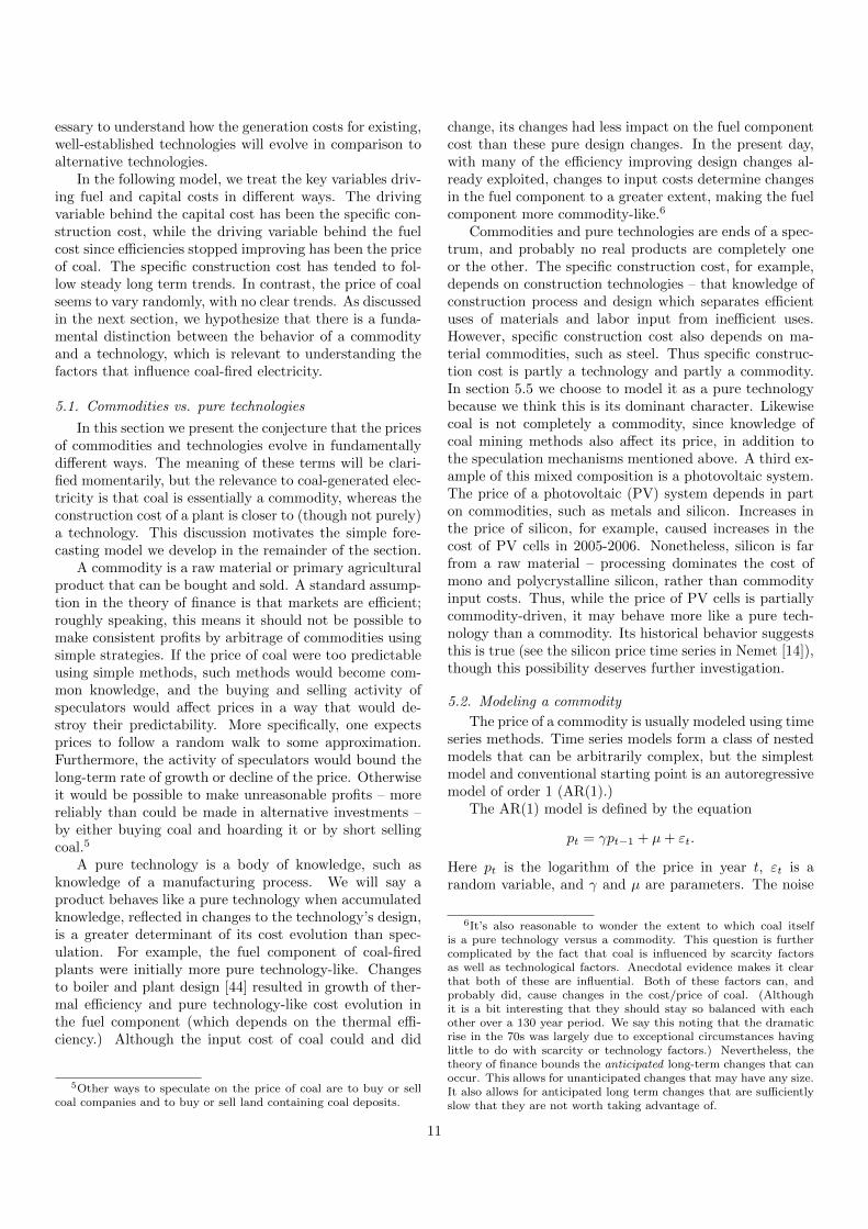
Figure 14: Extrapolation of capital costs 50 years into future. Insetshows a low-cost scenario for specific construction cost based on as-sumptions given in the text. Main axes show the resulting capitalcost after accounting for capacity factor and interest rate. Thesevariables are assumed to stay fixed at their 2006 values.

the generalized version of Moore’s law. We find the endresults yield similar predictions, and so choose to use anexponential in time because it is simpler.

One of the problems we confront in modeling the spe-cific capital cost is the break in the decreasing trend thatoccurs roughly in 1970, as shown in Figure 14. As alreadydiscussed in Section 2.5.1, roughly speaking the specificconstruction cost generally dropped from 1902 - 1970, in-creased until about 1990, and has been roughly flat orslightly decreasing since then. Pollution controls have beenproposed as the dominant cause of the increase in pricesthat occurs after 1970, though this is somewhat contro-versial. To make an extrapolation model we are forced tomake a choice as to how to treat the period of rising costs,and what its effect will be going forward.

Our main point in this paper is to show that, even un-der an optimistic point of view in which the constructioncost of coal plants substantially decreases, the price of coalwill dominate the cost of coal-fired electricity, and will im-pose a fluctuating floor below which it is unlikely to pen-etrate. Thus, in order to be as optimistic as is reasonablypossible about the future behavior of coal-fired electricityprices, we postulate a low cost scenario in which we as-sume that after 2006 the specific construction cost revertsto the same rate of exponential decrease that it had priorto 1970.

To implement this scenario we fit an exponential curveto the historical data only from 1902 - 1970, as shownin Figures 8 and 14. Then we generate an exponentialextrapolation having this same slope, but multiplied byan appropriate factor to have it start from the 2006 levelof specific construction cost (Fig. 14 inset.) We followa similar procedure for O&M costs. All other variablesused in the our cost equation are assumed to maintaintheir 2006 values. The resulting extrapolation provides acrude but simplified way of estimating potential baselinegeneration costs on the basis of historical experience.

The inset of Fig. 14 shows the specific construction

cost under the assumption that plants return to their pre-1970 rate of improvement, while the main axes show theresulting evolution of the amortized capital cost after ac-counting for the 2006 values of interest rate and capacityfactor. Under the low cost scenario, the capital cost wouldbe reduced 67% by 2056 to 0.82 ¢/kWh. This would stillplace it higher than the historical low of 0.56 ¢/kWh thatoccurred in 1968. (We omit the plot of the O&M extrapo-lation because it is less important, but we include its con-tribution in the total generation cost shown in Fig. 16.)

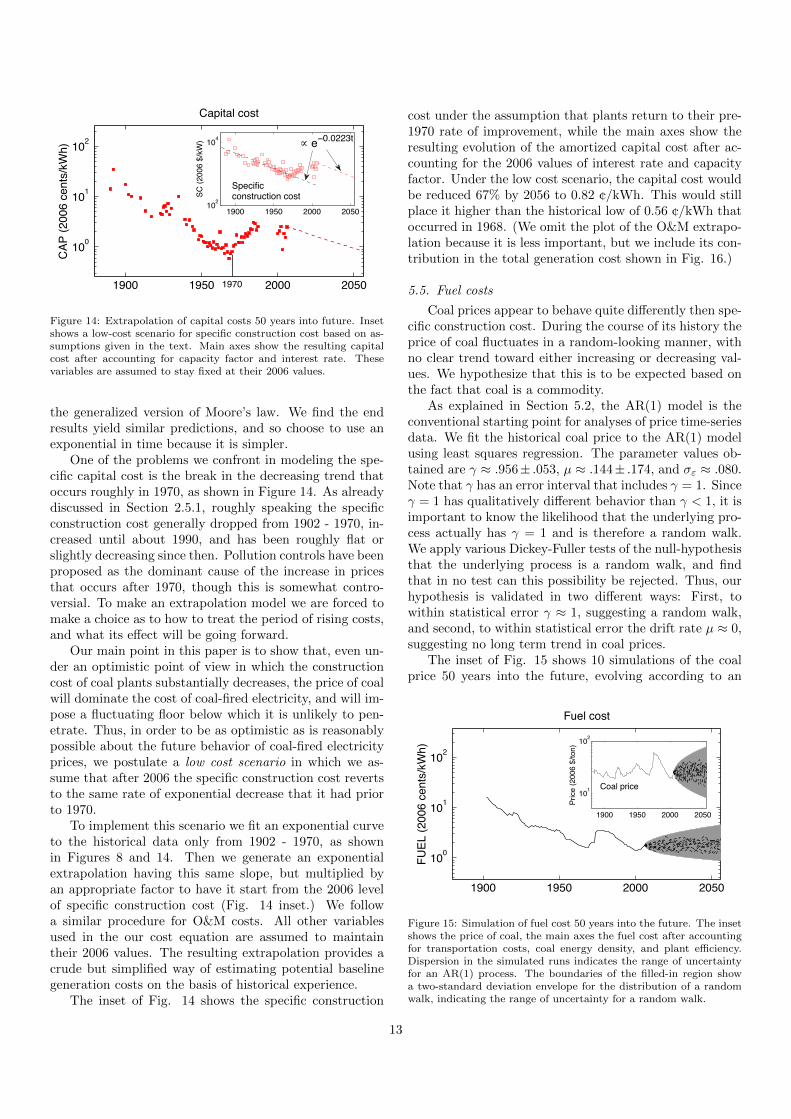
5.5. Fuel costs

Coal prices appear to behave quite differently then spe-cific construction cost. During the course of its history theprice of coal fluctuates in a random-looking manner, withno clear trend toward either increasing or decreasing val-ues. We hypothesize that this is to be expected based onthe fact that coal is a commodity.

As explained in Section 5.2, the AR(1) model is theconventional starting point for analyses of price time-seriesdata. We fit the historical coal price to the AR(1) modelusing least squares regression. The parameter values ob-tained are γ ≈ .956± .053, µ ≈ .144± .174, and σε ≈ .080.Note that γ has an error interval that includes γ = 1. Sinceγ = 1 has qualitatively different behavior than γ < 1, it isimportant to know the likelihood that the underlying pro-cess actually has γ = 1 and is therefore a random walk.We apply various Dickey-Fuller tests of the null-hypothesisthat the underlying process is a random walk, and findthat in no test can this possibility be rejected. Thus, ourhypothesis is validated in two different ways: First, towithin statistical error γ ≈ 1, suggesting a random walk,and second, to within statistical error the drift rate µ ≈ 0,suggesting no long term trend in coal prices.

The inset of Fig. 15 shows 10 simulations of the coalprice 50 years into the future, evolving according to an

1900 1950 2000 2050

100

101

102

FUEL

(200

6 ce

nts/

kWh)

Fuel cost

1900 1950 2000 2050

101

102

Price

(200

6 $/

ton)

Coal price

Figure 15: Simulation of fuel cost 50 years into the future. The insetshows the price of coal, the main axes the fuel cost after accountingfor transportation costs, coal energy density, and plant efficiency.Dispersion in the simulated runs indicates the range of uncertaintyfor an AR(1) process. The boundaries of the filled-in region showa two-standard deviation envelope for the distribution of a randomwalk, indicating the range of uncertainty for a random walk.

13

!"## !"$# %### %#$#!#!!

!##

!#!

!#%

&'()*+%##,*-./)(01234

5')67*-'()

*

*

5')67*-'()*+5&489.7*-'()*+8:;<4&6=>)67*-'()*+&?@4ABC*-'()*+AC4

1900 1950 2000 205010!1

100

101

102

Cost

(200

6 ce

nts/

kWh)

Total cost

Total cost (TC)Fuel cost (FUEL)Capital cost (CAP)O&M cost (OM)

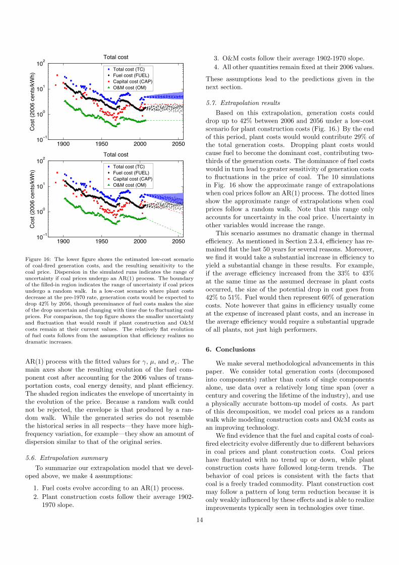
Figure 16: The lower figure shows the estimated low-cost scenarioof coal-fired generation costs, and the resulting sensitivity to thecoal price. Dispersion in the simulated runs indicates the range ofuncertainty if coal prices undergo an AR(1) process. The boundaryof the filled-in region indicates the range of uncertainty if coal pricesundergo a random walk. In a low-cost scenario where plant costsdecrease at the pre-1970 rate, generation costs would be expected todrop 42% by 2056, though preeminance of fuel costs makes the sizeof the drop uncertain and changing with time due to fluctuating coalprices. For comparison, the top figure shows the smaller uncertaintyand fluctuation that would result if plant construction and O&Mcosts remain at their current values. The relatively flat evolutionof fuel costs follows from the assumption that efficiency realizes nodramatic increases.

AR(1) process with the fitted values for γ, µ, and σε. Themain axes show the resulting evolution of the fuel com-ponent cost after accounting for the 2006 values of trans-portation costs, coal energy density, and plant efficiency.The shaded region indicates the envelope of uncertainty inthe evolution of the price. Because a random walk couldnot be rejected, the envelope is that produced by a ran-dom walk. While the generated series do not resemblethe historical series in all respects—they have more high-frequency variation, for example—they show an amount ofdispersion similar to that of the original series.

5.6. Extrapolation summary

To summarize our extrapolation model that we devel-oped above, we make 4 assumptions:

1. Fuel costs evolve according to an AR(1) process.

2. Plant construction costs follow their average 1902-1970 slope.

3. O&M costs follow their average 1902-1970 slope.

4. All other quantities remain fixed at their 2006 values.

These assumptions lead to the predictions given in thenext section.

5.7. Extrapolation results

Based on this extrapolation, generation costs coulddrop up to 42% between 2006 and 2056 under a low-costscenario for plant construction costs (Fig. 16.) By the endof this period, plant costs would would contribute 29% ofthe total generation costs. Dropping plant costs wouldcause fuel to become the dominant cost, contributing two-thirds of the generation costs. The dominance of fuel costswould in turn lead to greater sensitivity of generation coststo fluctuations in the price of coal. The 10 simulationsin Fig. 16 show the approximate range of extrapolationswhen coal prices follow an AR(1) process. The dotted linesshow the approximate range of extrapolations when coalprices follow a random walk. Note that this range onlyaccounts for uncertainty in the coal price. Uncertainty inother variables would increase the range.

This scenario assumes no dramatic change in thermalefficiency. As mentioned in Section 2.3.4, efficiency has re-mained flat the last 50 years for several reasons. Moreover,we find it would take a substantial increase in efficiency toyield a substantial change in these results. For example,if the average efficiency increased from the 33% to 43%at the same time as the assumed decrease in plant costsoccurred, the size of the potential drop in cost goes from42% to 51%. Fuel would then represent 60% of generationcosts. Note however that gains in efficiency usually comeat the expense of increased plant costs, and an increase inthe average efficiency would require a substantial upgradeof all plants, not just high performers.

6. Conclusions

We make several methodological advancements in thispaper. We consider total generation costs (decomposedinto components) rather than costs of single componentsalone, use data over a relatively long time span (over acentury and covering the lifetime of the industry), and usea physically accurate bottom-up model of costs. As partof this decomposition, we model coal prices as a randomwalk while modeling construction costs and O&M costs asan improving technology.

We find evidence that the fuel and capital costs of coal-fired electricity evolve differently due to different behaviorsin coal prices and plant construction costs. Coal priceshave fluctuated with no trend up or down, while plantconstruction costs have followed long-term trends. Thebehavior of coal prices is consistent with the facts thatcoal is a freely traded commodity. Plant construction costmay follow a pattern of long term reduction because it isonly weakly influenced by these effects and is able to realizeimprovements typically seen in technologies over time.

14

Such a difference in the behavior of coal prices andplant construction costs would yield different behavior forthe fuel and capital cost components. Although histori-cally both the fuel and capital components improved atsimilar rates, the main driver of improvement in fuel costs– thermal efficiency – has been unchanged since the early1960s. Without a substantial improvement in the averagethermal efficiency, the main driver of change in fuel costswould be the coal price. Under a low-cost scenario wherecapital costs were driven down by improving plant con-struction costs, the total generation cost would decreaseabout 40% over the next 50 years. Coal prices, in con-trast, are statistically neither decreasing nor increasing,and so provide a statistically fluctuating floor on the over-all generation cost, with no clear long-term trend.

Although all the analysis in this paper is specific tocoal, we hypothesize that a similar analysis might applyto other fuel-based sources of electricity, such as naturalgas. In fact, because natural gas and oil are both traded onexchanges, with standardized futures contracts, it is easierto speculate in them than it is in coal. Thus we wouldexpect that the commodity part of our model will applyto them even more strongly. This would suggest that themajor non-renewable sources of electricity should all hit anoisy floor, similar to the one we have postulated here forcoal.

7. Acknowledgments

This material is based upon work supported by the Na-tional Science Foundation under Grant No. 0624351 (thisis the Financial Markets grant no). Any opinions, findings,and conclusions or recommendations expressed in this ma-terial are those of the author(s) and do not necessarily re-flect the views of the National Science Foundation. Wethank Margaret Alexander and Tim Taylor for substantialhelp obtaining source materials. We thank Arnulf Grublerfor helpful conversations and suggestions. We thank Char-lie Wilson for several valuable conversations and extensivefeedback on an early draft, and Dan Schrag for a challengethat led to the idea for this paper.

A. Change decomposition

Consider the following problem. We have a functionf = f(x, y), and during some period of time f changesas a result of simultaneous changes to x and y. We wantto know how much of the change to f each variable is“responsible for.”

To be more precise, let ∆f be the change in f . Wewould like to decompose ∆f into 2 terms, correspondingto the change contributed by each variable:

∆f = ∆fx + ∆fy,

where ∆fi denotes the change in f resulting from thechange in i. A way to do this decomposition is suggested

by the calculus identity

df =∂f

∂xdx+

∂f

∂ydy.

The trick is to generalize this expression to finite ratherthan infinitesimal changes. More to the point, we needto be able to take common combinations of variables –e.g. products, quotients – and express changes to thesecombinations in ways appropriate for finite differences.

For example, consider a product of two variables, f(x, y) =xy. The differential f is

df = x dy + y dx

suggesting the decomposition for finite differences is ∆f =x∆y + y∆x. However, the correct expression is

∆f = x∆y + y∆x+ ∆x∆y.

In addition to the two expected terms, a third cross termcontaining both differences appears. As the differencesbecome small, the cross term will vanish more quicklythan the other terms, recovering the calculus limit df =x dy+ y dx. However, for finite differences, the cross termpotentially introduces a large residual if ignored.

In order to decompose the change in f into just 2pieces, we evenly split the cross term into the other terms:

∆f = x∆y +1

2∆x∆y + y∆x+

1

2∆x∆y

= (x+1

2∆x)∆y + (y +

1

2∆y)∆x

The first term may be interpreted as the change in f dueto change in y; the second as the change in f due to changein x. We therefore have our desired decomposition for thecase of products of 2 variables:

∆fx ≡ (y +1

2∆y)∆x

∆fy ≡ (x+1

2∆x)∆y

which by construction has the desired property ∆f =∆fx + ∆fy. Similar rules can be derived for products of 3or more variables, for quotients, and other expressions.

References

[1] World bank development indicators database (2008).[2] Key world energy statistics, Tech. rep., International Energy

Agency (2008).[3] R. Kumiya, Technological progress and the production func-

tion in the united states steam power industry, The Review ofEconomics and Statistics 44 (2) (1962) 156–166.

[4] M. Nerlove, Returns to scale in electricity supply, in: Mea-surement in economics: studies in mathematical economics andeconometrics, Stanford University, Stanford, 1963.

[5] T. G. Cowing, Technical change and scale economies in an engi-neering production function: The case of steam electric power,The Journal of Industrial Economics 23 (2) (1974) 135–152.

15

[6] L. R. Christensen, W. H. Greene, Economies of scale in U.S.electric power generation, The Journal of Political Economy84 (4) (1976) 655–676.

[7] D. A. Huettner, J. H. Landon, Electric utilities: Scale economiesand diseconomies, Southern Economic Journal 44 (4) (1978)883–912.

[8] J. F. Stewart, Plant size, plant factor, and the shape of the av-erage cost function in electric power, The Bell Journal of Eco-nomics 10 (2) (1979) 549–565.

[9] R. A. Nelson, M. E. Wohar, Regulation, scale economies, andproductivity in steam-electric generation, International Eco-nomic Review 24 (1) (1983) 57–59.

[10] F. M. Gollop, M. J. Roberts, Environmental regulations andproductivity growth: The case of fossil-fueled electric powergeneration, Journal of Political Economy 91 (4) (1983) 654–674.

[11] P. L. Joskow, N. L. Rose, The effects of technological change, ex-perience, and environmental regulation on the construction costof coal-burning generating units, Rand Journal of Economics16 (1) (1985) 1–27.

[12] M. J. McCabe, Principals, agents, and the learning curve: Thecase of steam-electric power plant design and construction, TheJournal of Industrial Economics 44 (4) (1996) 357–375.

[13] J. J. Hisnanick, K. O. Kymn, Modeling economies of scale:the case of US electric power companies, Energy Economics 21(1999) 225–237.

[14] G. F. Nemet, Beyond the learning curve: factors influencingcost reductions in photovoltaics, Energy Policy 34 (2006) 3218–3232.

[15] A study of coal prices, Tech. Rep. NP-20948, Council on Wageand Price Stability, Washington, DC (1976).

[16] R. S. Manthy, J. R. Tron, Natural Resource Commodities—ACentury of Statistics, Johns Hopkins, Baltimore, 1978.

[17] Annual energy review, Tech. Rep. DOE/EIA-0384(2006), En-ergy Information Administration (2006).

[18] S. H. Schurr, B. C. Netschert, Energy in the American econ-omy, 1850-1975: an economic study of its history and prospects,Johns Hopkins, Baltimore, 1960.

[19] Mineral yearbook, Tech. rep., US Geological Survey, Washing-ton, DC (various issues 1932-1976).

[20] Historical Statistics of the Electric Utility Industry through1992, Edison Electric Institute, Washington, DC, 1995.

[21] Encyclopaedia britannica (2009) [cited September 19, 2009].URL http://www.britannica.com/EBchecked/topic/615316/

unit-train

[22] Steam-electric plant construction cost and annual productionexpenses for 1947, Tech. rep., Federal Power Commission(1947).

[23] R. F. Hirsh, Technology and Transformation in the AmericanElectric Utility Industry, Cambridge, 2002.

[24] C. E. Neil, Entering the seventh decade of electric power, EdisonElectric Insitute Bulletin 10 (9).

[25] Steam-electric plant construction cost and annual productionexpenses, Tech. Rep. FPC S-154, Federal Power Commission(1961).

[26] Steam-electric plant construction cost and annual productionexpenses, Tech. Rep. DOE/EIA-0033(78), Energy InformationAdministration (1978).

[27] Thermal-electric plant construction cost and annual productionexpenses, Tech. Rep. DOE/EIA-0323(79), Energy InformationAdministration (1979).

[28] A. Beamon, T. J. Leckey, Trends in power plant operating costs,Tech. Rep. EIA/DOE-0607, Energy Information Administra-tion (1999).URL http://www.eia.doe.gov/oiaf/issues/opctbl2.html

[29] U.S. electricity production costs and components (1995-2007),Tech. rep., Nuclear Energy Institute.URL http://www.nei.org/resourcesandstats/

documentlibrary/reliableandaffordableenergy/

graphicsandcharts/uselectricityproductioncostsandcomponents/

[30] S. Yeh, E. S. Rubin, A centurial history of technological changeand learning curves for pulverized coal-fired utility boilers, En-

ergy 32 (10) (2007) 1996–2005.[31] P. Sporn, Vistas in Electric Power, Pergamon, Oxford, 1968.[32] C. Komonoff, Power Plant Cost Escalation: Nuclear and Coal

Capital Costs, Regulation, and Economics, Van Nostrand, NewYork, 1981.

[33] Historical plant cost and annual production expenses for se-lected plants, Tech. Rep. DOE/EIA-0455(82), Energy Informa-tion Administration (1982).

[34] Historical plant cost and annual production expenses for se-lected plants, Tech. Rep. DOE/EIA-0455(87), Energy Informa-tion Administration (1987).

[35] E. Shuster, Tracking new coal-fired power plants, Tech. rep.,National Energy Technology Laboratory (2007).

[36] B. L. Cohen, The Nuclear Energy Option, Plenum, New York,1992.

[37] G. M. Masters, Renewable and Efficient Electric Power Systems,John Wiley, Hoboken, 2004.

[38] Platts UDI world electric power plants data base.[39] Census of electrical industries, Tech. rep., Census Bureau,

Washington, DC (various issues 1902-1937).[40] H. Wynne, Tech. rep., Sanford C. Bernstein & Co. LLC (2008).[41] Statistics of privately owned electric utilities in the united

states, Tech. Rep. FPC S-247, Federal Power Commission(1973).

[42] Federal reserve statistical release H.15.[43] The future of coal, Tech. rep., Massachusetts Institute of Tech-

nology (2007).[44] B. . Veatch, Power Plant Engineering, Springer Science, New

York, 1996.[45] W. C. Gavin Sinclair, Steven Klepper, What’s experience got

to do with it? sources of cost reduction in a large specialtychemical producer, Management Science 46 (1) (2000) 28–45.

[46] J. M. Dutton, A. Thomas, Treating progress functions as amanagerial opportunity, Acadamy of Management Review 9 (2)(1984) 235–247.

[47] P. Thompson, Handbook of Economics of Technical Change,Elsevier/North Holland, 2009, Ch. Learning By Doing.

[48] J. D. Farmer, J. E. Trancik, Dynamics of technological devel-opment in the energy sector, in: J. P. Onstwedder, M. Mainelli(Eds.), London Accord Final Publication, 2007.

[49] J. F. Muth, Search theory and the manufacturing progress func-tion, Management Science 32 (8) (1986) 948–962.

[50] J. McNerney, J. D. Farmer, S. Redner, J. E. Trancik, The roleof design complexity in technology improvement.

[51] B. Nagy, J. D. Farmer, J. E. Trancik, More than moore: Com-paring forecasts of technological progress (in preparation).

[52] D. Sahal, Patterns of Technological Innovation, Addison-Wesley, London, 1981.

[53] W. J. Abernathy, K. Wayne, Limits of the learning curve, Har-vard Business Review.

16