Historic Wildfire Research in Southeastern Idaho

Fredrik Thoren, kiruna_thoren@hotmail.comDaniel Mattsson, phillou1@hotmail.com

Abstract: The goal of this project was to create and analyze wildfire areas that occurred on BLMland in eastern Snake River Plan between 1939-1997. We began with hand drawn wildfire mapsand digitized them using standard heads-up digitizing techniques. Our Area Of Concern wassoutheast Idaho which includes Pocatello and Idaho Falls. We then analyzed the size of fireareas, proportion of vegetation types burned, fire frequency, and fire intervals. These problemswere solved using raster grid and vector polygon methods. The results show an overalldecreasing trend in acres burned from 1939-1997. Problems associated with decreasing fireacreage are discussed.

Keywords: GIS, fires, BLM, Idaho.

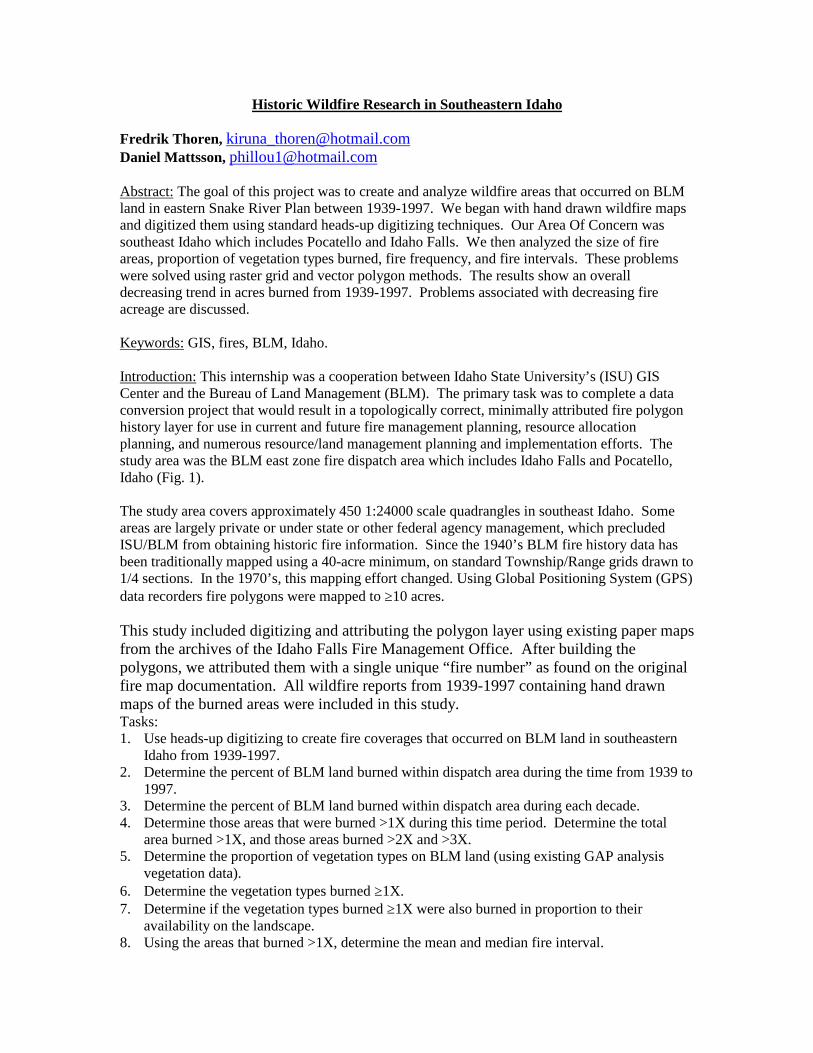
Introduction: This internship was a cooperation between Idaho State University’s (ISU) GISCenter and the Bureau of Land Management (BLM). The primary task was to complete a dataconversion project that would result in a topologically correct, minimally attributed fire polygonhistory layer for use in current and future fire management planning, resource allocationplanning, and numerous resource/land management planning and implementation efforts. Thestudy area was the BLM east zone fire dispatch area which includes Idaho Falls and Pocatello,Idaho (Fig. 1).

The study area covers approximately 450 1:24000 scale quadrangles in southeast Idaho. Someareas are largely private or under state or other federal agency management, which precludedISU/BLM from obtaining historic fire information. Since the 1940’s BLM fire history data hasbeen traditionally mapped using a 40-acre minimum, on standard Township/Range grids drawn to1/4 sections. In the 1970’s, this mapping effort changed. Using Global Positioning System (GPS)data recorders fire polygons were mapped to ≥10 acres.

This study included digitizing and attributing the polygon layer using existing paper mapsfrom the archives of the Idaho Falls Fire Management Office. After building thepolygons, we attributed them with a single unique “fire number” as found on the originalfire map documentation. All wildfire reports from 1939-1997 containing hand drawnmaps of the burned areas were included in this study.Tasks:1. Use heads-up digitizing to create fire coverages that occurred on BLM land in southeastern

Idaho from 1939-1997.2. Determine the percent of BLM land burned within dispatch area during the time from 1939 to

1997.3. Determine the percent of BLM land burned within dispatch area during each decade.4. Determine those areas that were burned >1X during this time period. Determine the total

area burned >1X, and those areas burned >2X and >3X.5. Determine the proportion of vegetation types on BLM land (using existing GAP analysis

vegetation data).6. Determine the vegetation types burned ≥1X.7. Determine if the vegetation types burned ≥1X were also burned in proportion to their

availability on the landscape.8. Using the areas that burned >1X, determine the mean and median fire interval.

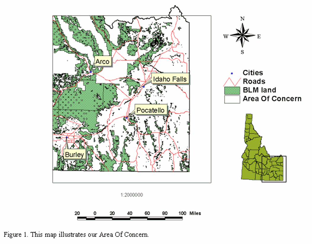
Methods:All file names are described in Appendix A.1. To digitize the fire areas we used ArcView. All reports contained hand drawn maps. In morerecent years (1970-1997) these are drawn on a topographic map background. By using DigitalRaster Graphics (DRG) of the area we could find the fire area specified on the DRG and theneasier digitize these areas. Earlier reports only contain the Township/ Range/ Section identifiers.We created a new shape file for each year. We added the following fields to the attribute table:fire_year (containing the fire year in two digits), fire_number (an alphanumeric fire numberassigned by the BLM and provided on fire documentation forms). We also calculated the area,perimeter and acreage of each fire polygon (Table 1).

In some years, fires occurred ≥1X in the same area. To address this problem we created twoshape files for that year (e.g., one was called fire_64.shp and the next was called fire_641.shp).To deliver this information to the BLM we converted the shape files into ArcInfo coverages usingan aml called shape2arc.aml. After this, the coverages were exported as interchange files.

2. We MERGED all themes together in ArcView and created a theme called mergeny.shp. Wethen CLIPPED this theme with aocblm.shp (which contains BLM land within our area ofconcern) and a shape file showing the dispatch area to produce a coverage containing only fireson BLM land within the dispatch area. We exported the database tables to Excel to determine theproportion of land burned on BLM land within the dispatch area.

3. Next we selected fires from each decade and calculated acreage using methods described in 2(above).

4. The most difficult task was determining fire frequency. For this we used two approaches. Thefirst approach was to use raster grids. All fire coverages were rasterized using a new field calledz for the pixel’s digital number (Table 1). This Boolean field indicates where there has been afire. Areas where a fire had occurred were given a value of 1. This also required that weRECLASS all grids so NoData pixels were assigned a 0. All grids were added together with theMAP CALCULATOR. This resulted in a grid called gridallf with grid cells indicating thenumber of times each pixel had burned. From this grid we could query the areas that had burned>1X etc. To determine the acreage that had burned >1X we exported the database files to exceland calculated area.

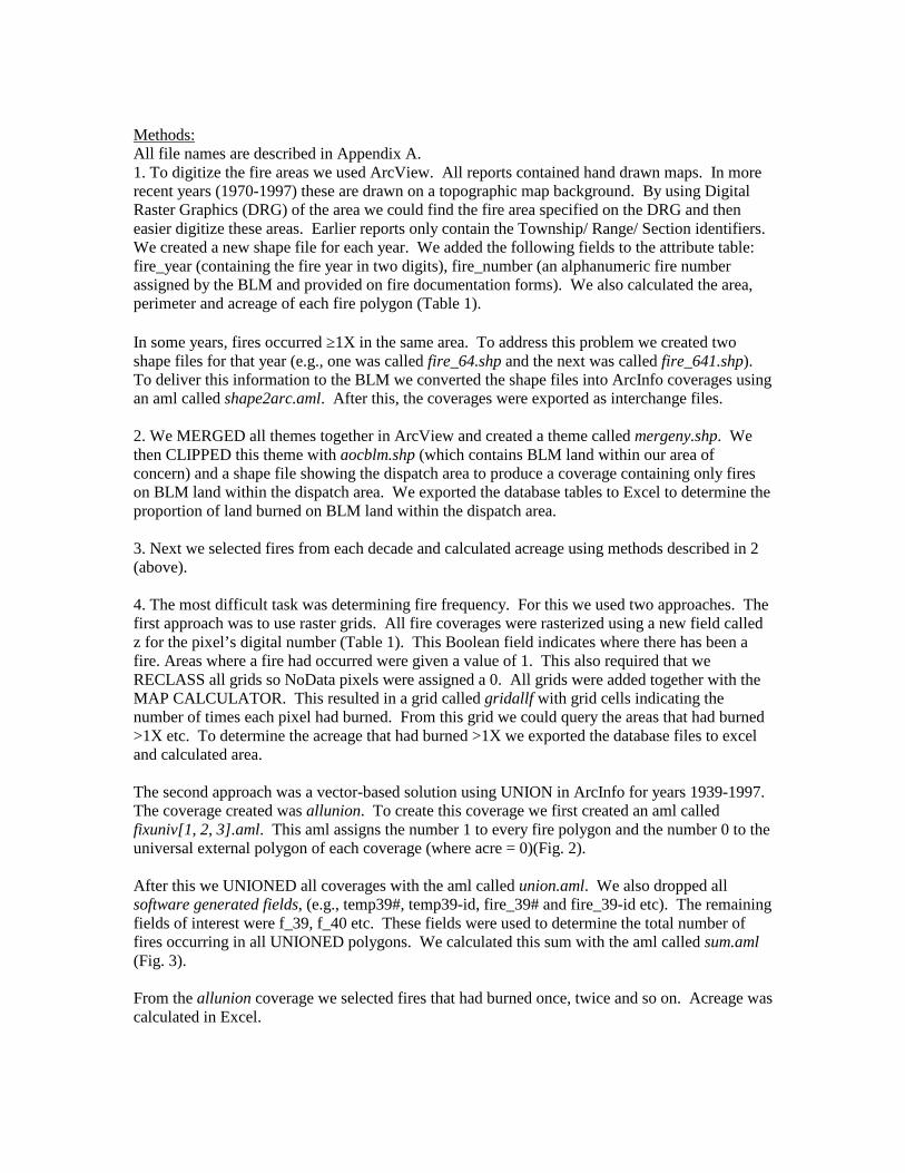
The second approach was a vector-based solution using UNION in ArcInfo for years 1939-1997.The coverage created was allunion. To create this coverage we first created an aml calledfixuniv[1, 2, 3].aml. This aml assigns the number 1 to every fire polygon and the number 0 to theuniversal external polygon of each coverage (where acre = 0)(Fig. 2).

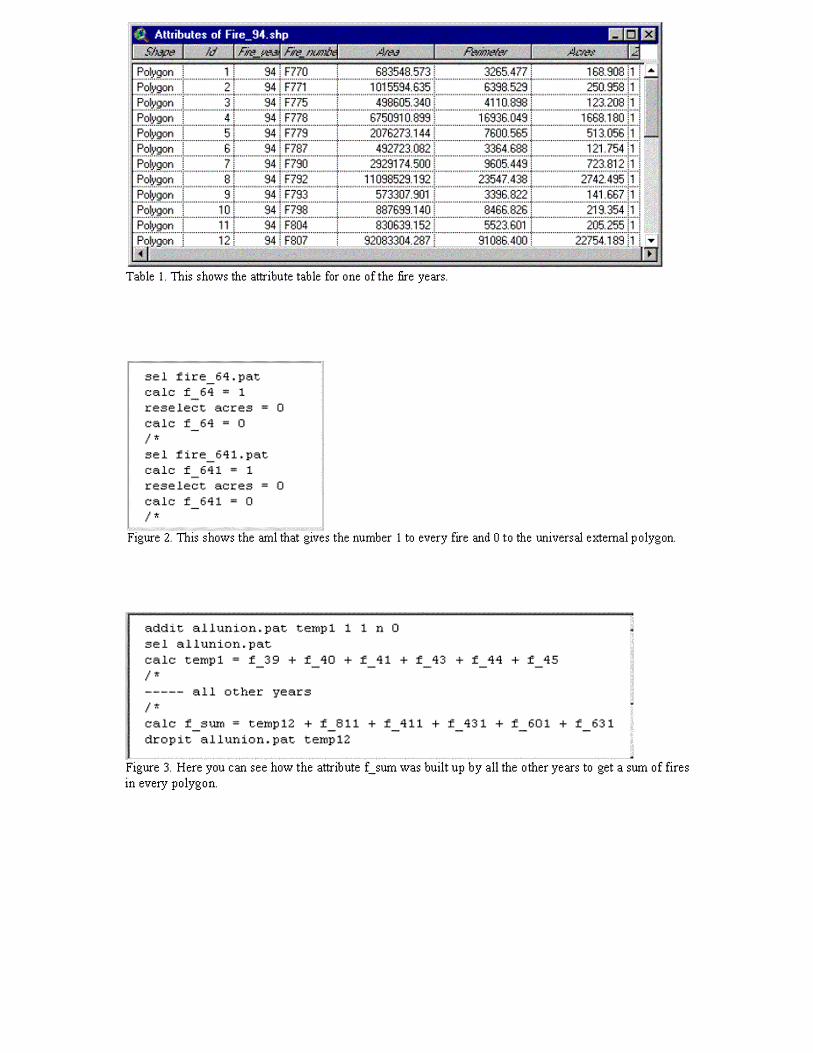
After this we UNIONED all coverages with the aml called union.aml. We also dropped allsoftware generated fields, (e.g., temp39#, temp39-id, fire_39# and fire_39-id etc). The remainingfields of interest were f_39, f_40 etc. These fields were used to determine the total number offires occurring in all UNIONED polygons. We calculated this sum with the aml called sum.aml(Fig. 3).

From the allunion coverage we selected fires that had burned once, twice and so on. Acreage wascalculated in Excel.

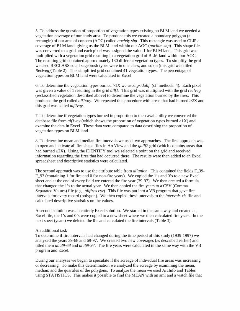
5. To address the question of proportion of vegetation types existing on BLM land we needed avegetation coverage of our study area. To produce this we created a boundary polygon (arectangle) of our area of concern (AOC) called aocbdy.shp. This rectangle was used to CLIP acoverage of BLM land, giving us the BLM land within our AOC (aocblm.shp). This shape filewas converted to a grid and each pixel was assigned the value 1 for BLM land. This grid wasmultiplied with a vegetation grid resulting in a vegetation grid of BLM land within our AOC.The resulting grid contained approximately 130 different vegetation types. To simplify the gridwe used RECLASS so all sagebrush types were in one class, and so on (this grid was titledReclveg)(Table 2). This simplified grid contained 41 vegetation types. The percentage ofvegetation types on BLM land were calculated in Excel.

6. To determine the vegetation types burned >1X we used gridallf (cf. methods: 4). Each pixelwas given a value of 1 resulting in the grid allf1. This grid was multiplied with the grid reclveg(reclassified vegetation described above) to determine the vegetation burned by the fires. Thisproduced the grid called alf1vny. We repeated this procedure with areas that had burned ≥2X andthis grid was called alf2vny.

7. To determine if vegetation types burned in proportion to their availability we converted thedatabase file from alf1vny (which shows the proportion of vegetation types burned ≥1X) andexamine the data in Excel. These data were compared to data describing the proportion ofvegetation types on BLM land.

8. To determine mean and median fire intervals we used two approaches. The first approach wasto open and activate all fire shape files in ArcView and the gallf2 grid (which contains areas thathad burned ≥2X). Using the IDENTIFY tool we selected a point on the grid and receivedinformation regarding the fires that had occurred there. The results were then added to an Excelspreadsheet and descriptive statistics were calculated.

The second approach was to use the attribute table from allunion. This contained the fields F_39-F_97 (containing 1 for fire and 0 for non-fire years). We copied the 1’s and 0’s to a new Excelsheet and at the end of every field we entered the fire year (39-97). We then created a formulathat changed the 1’s to the actual year. We then copied the fire years to a CSV (CommaSeparated Values) file (e.g., allfires.csv). This file was put into a VB program that gave fireintervals for every record (polygon). We then copied these intervals to the intervals.xls file andcalculated descriptive statistics on the values.

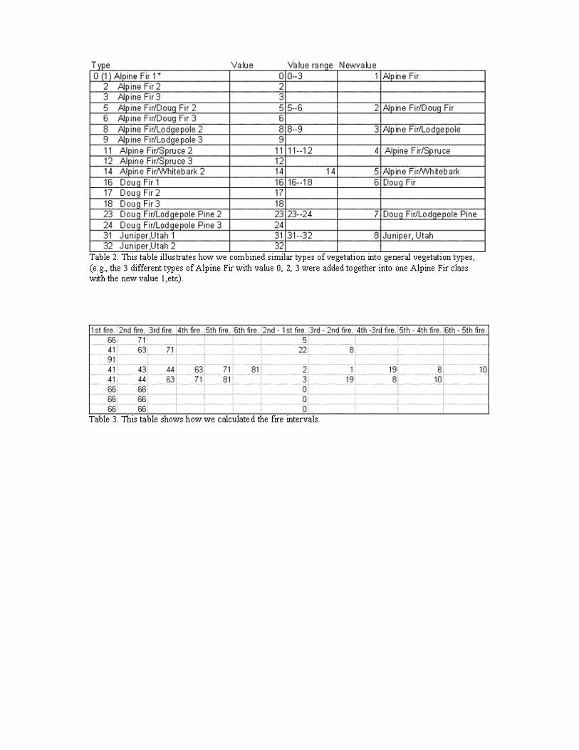
A second solution was an entirely Excel solution. We started in the same way and created anExcel file, the 1’s and 0’s were copied to a new sheet where we then calculated fire years. In thenext sheet (years) we deleted the 0’s and calculated the fire intervals (Table 3).

An additional taskTo determine if fire intervals had changed during the time period of this study (1939-1997) weanalyzed the years 39-68 and 69-97. We created two new coverages (as described earlier) andtitled them uni39-68 and uni69-97. The fire years were calculated in the same way with the VBprogram and Excel.

During our analyses we began to speculate if the acreage of individual fire areas was increasingor decreasing. To make this determination we analyzed the acreage by examining the mean,median, and the quartiles of the polygons. To analyze the mean we used ArcInfo and Tablesusing STATISTICS. This makes it possible to find the MEAN with an aml and a watch file that

wrote all output to a text file. This text file was opened in Excel and a chart was createdillustrating the mean acres burned each decade.To analyze the median we again used an aml that writes the acreage of each fire to a watch file.To calculate the median we used Excel. To determine quartiles we used a program called boxplot.This program takes a dbf file with acres and calculates median, 1st, and 3rd quartiles. The inputdbf files were created from the second watch file, described above.

Results:The results of digitizing and the location of each coverage is given in Appendix A.

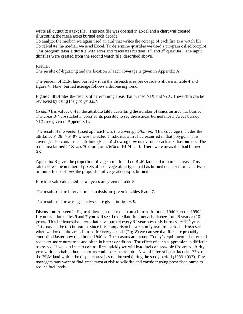
The percent of BLM land burned within the dispatch area per decade is shown in table 4 andfigure 4. Note: burned acreage follows a decreasing trend.

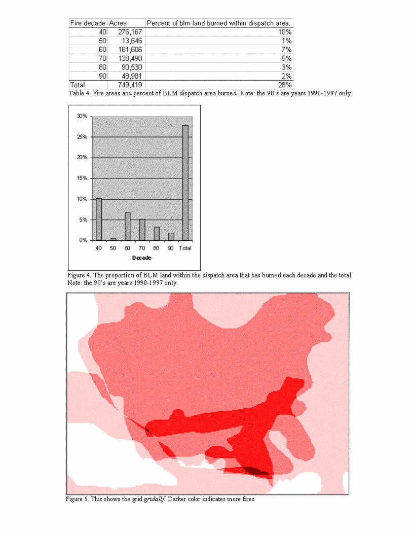
Figure 5 illustrates the results of determining areas that burned >1X and >2X. These data can bereviewed by using the grid gridallf.

Gridallf has values 0-4 in the attribute table describing the number of times an area has burned.The areas 0-4 are scaled in color so its possible to see those areas burned most. Areas burned>1X, are given in Appendix B.

The result of the vector-based approach was the coverage allunion. This coverage includes theattributes F_39 -> F_97 where the value 1 indicates a fire had occurred in that polygon. Thiscoverage also contains an attribute (F_sum) showing how many times each area has burned. Thetotal area burned >1X was 702 km2, or 3.56% of BLM land. There were areas that had burned6X.

Appendix B gives the proportion of vegetation found on BLM land and in burned areas. Thistable shows the number of pixels of each vegetation type that has burned once or more, and twiceor more. It also shows the proportion of vegetation types burned.

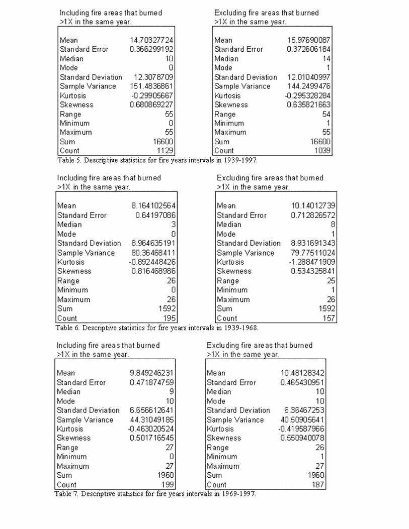
Fire intervals calculated for all years are given in table 5.

The results of fire interval trend analysis are given in tables 6 and 7.

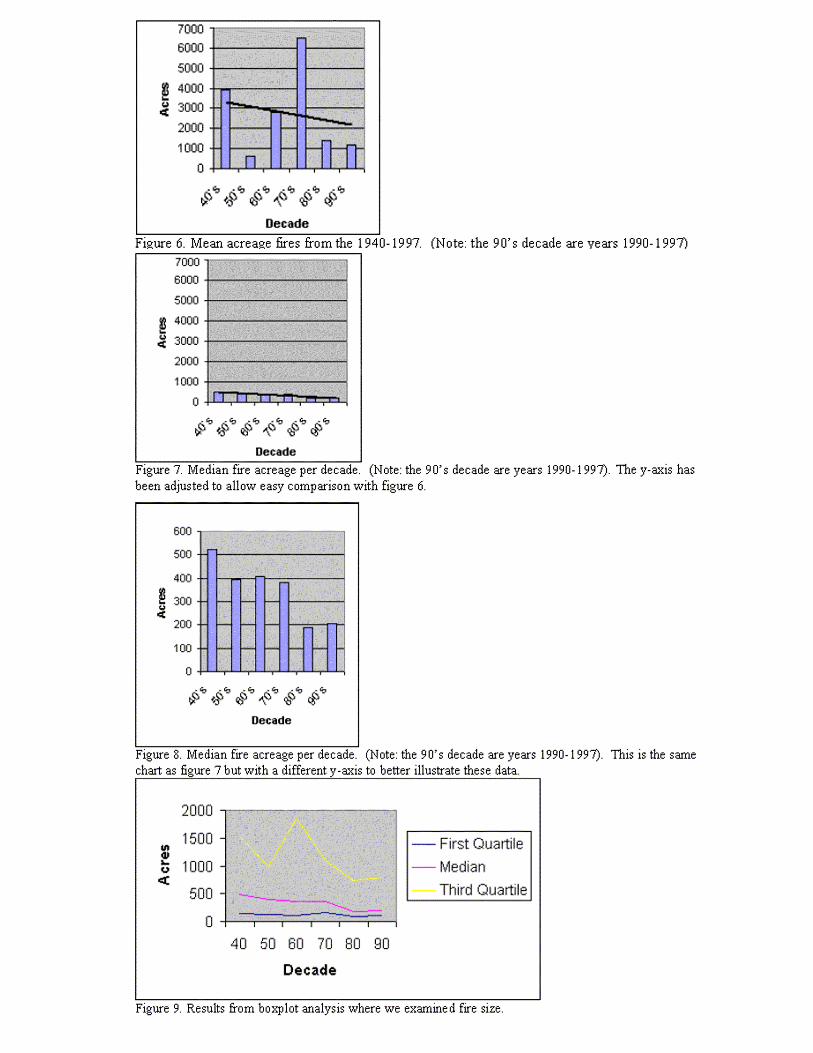
The results of fire acreage analyses are given in fig’s 6-9.

Discussion: As seen in figure 4 there is a decrease in area burned from the 1940’s to the 1990’s.If you examine tables 6 and 7 you will see the median fire intervals change from 8 years to 10years. This indicates that areas that have burned every 8th year now only burn every 10th year.This may not be too important since it is comparison between only two fire periods. However,when we look at the areas burned for every decade (Fig. 8) we can see that fires are probablycontrolled faster now than in the 1940’s. The reasons are many. Today’s equipment is better androads are more numerous and often in better condition. The effect of such suppression is difficultto assess. If we continue to control fires quickly we will load fuels on possible fire areas. A dryyear with inevitable thunderstorms could be catastrophic. Also of interest is the fact that 72% ofthe BLM land within the dispatch area has not burned during the study period (1939-1997). Firemanagers may want to find areas most at risk to wildfire and consider using prescribed burns toreduce fuel loads.

Assessment of Errors and Bias: The reports used to digitize may not be consistent becausedifferent people who approximate area and reported acreage differently made them (Appendix C).The accuracy of the report varies a great deal from the beginning to the end. One thing toconsider is that the person who drew the map probably was not thinking about the possibility thatthe maps would be further analyzed. Even though there are some parts with poor accuracy wedon not think that it affects our discussion of whether fire acreage has decreased. Further, thesemaps are still the best information available.

Appendix A

Files in d:\data\blm_fire.Example:Name of the file: (explanation how the name is shortened) A description of the file.Where to find the file.

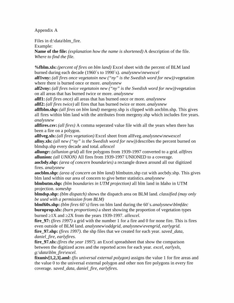
%fblm.xls: (percent of fires on blm land) Excel sheet with the percent of BLM landburned during each decade (1960`s to 1990`s). analysnew\newexcelalf1vny: (all fires once vegetatoin new (“ny” is the Swedish word for new)) vegetationwhere there is burned once or more. analysnewalf2vny: (all fires twice vegetatoin new (“ny” is the Swedish word for new)) vegetationon all areas that has burned twice or more. analysnewallf1: (all fires once) all areas that has burned once or more. analysnewallf2: (all fires twice) all fires that has burned twice or more. analysnewallfblm.shp: (all fires on blm land) mergeny.shp is clipped with aocblm.shp. This givesall fires within blm land with the attributes from mergeny.shp which includes fire years.analysnewallfires.csv: (all fires) A comma seperated value file with all the years when there hasbeen a fire on a polygon.allfveg.xls: (all fires vegetation) Excel sheet from allfveg. analysnew\newexcelallny.xls: (all new (“ny” is the Swedish word for new)) describes the percent burned onblmdsp.shp every decade and total. allexcelallungr: (allunion grid) all fire polygons from 1939-1997 converted to a grid. allfiresallunion: (all UNION) All fires from 1939-1997 UNIONED to a coverage.aocbdy.shp: (area of concern boundaries) a rectangle drawn around all our digitizedfires. analysnewaocblm.shp: (area of concern on blm land) blmbutm.shp cut with aocbdy.shp. This givesblm land within our area of concern to give better statistics. analysnewblmbutm.shp: (blm boundaries in UTM projection) all blm land in Idaho in UTMprojection. someshpblmdsp.shp: (blm dispatch) shows the dispatch area on BLM land. classified (may onlybe used with a permission from BLM)blmf60s.shp: (blm fires 60`s) fires on blm land during the 60`s. analysnew\blmfdecburnprop.xls: (burn proportions) a sheet showing the proportion of vegetation typesburned ≥1X and ≥2X from the years 1939-1997. allexcel.fire_97: (fires 1997) a grid with the number 1 for a fire and 0 for none fire. This is fireseven outside of BLM land. analysnew\oddgrid, analysnew\evengrid, earlygrid.fire_97.shp: (fires 1997). the shp files that we created for each year. saved_data,daniel_fire, earlyfires.fire_97.xls: (fires the year 1997). an Excel spreadsheet that show the comparisonbetween the digitized acres and the reported acres for each year. excel, earlyxls,g:\data\blm_fire\excel.fixuniv[1,2,3].aml: (fix universal external polygon) assigns the value 1 for fire areas andthe value 0 to the universal external polygon and other non fire polygons in every firecoverage. saved_data, daniel_fire, earlyfires.

Appendix A

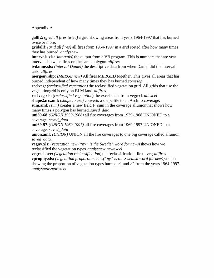
gallf2: (grid all fires twice) a grid showing areas from years 1964-1997 that has burnedtwice or more.gridallf: (grid all fires) all fires from 1964-1997 in a grid sorted after how many timesthey has burned. analysnewintervals.xls: (intervals) the output from a VB program. This is numbers that are yearintervals between fires on the same polygon. allfiresivdanne.xls: (interval Daniel) the descriptive data from when Daniel did the intervaltask. allfiresmergeny.shp: (MERGE new) All fires MERGED together. This gives all areas that hasburned independent of how many times they has burned. someshpreclveg: (reclassified vegetation) the reclassified vegetation grid. All grids that use thevegetationgrid is only on BLM land. allfiresreclveg.xls: (reclassified vegetation) the excel sheet from vegrecl. allexcelshape2arc.aml: (shape to arc) converts a shape file to an ArcInfo coverage.sum.aml: (sum) creates a new field F_sum in the coverage allunion that shows howmany times a polygon has burned. saved_data.uni39-68:(UNION 1939-1968) all fire coverages from 1939-1968 UNIONED to acoverage. saved_datauni69-97:(UNION 1969-1997) all fire coverages from 1969-1997 UNIONED to acoverage. saved_dataunion.aml: (UNION) UNION all the fire coverages to one big coverage called allunion.saved_data.vegny.xls: (vegetation new (“ny” is the Swedish word for new)) shows how wereclassified the vegetation types. analysnew\newexcelvegrecl.avc: (vegetation reclassification) the reclassification file to veg. allfiresvpropny.xls: (vegetation proportions new(“ny” is the Swedish word for new)) a sheetshowing the proportion of vegetation types burned ≥1 and ≥2 from the years 1964-1997.analysnew\newexcel

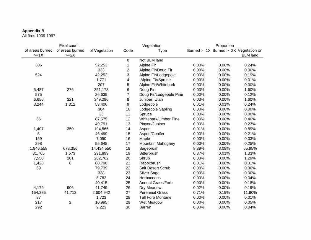
Appendix BAll fires 1939-1997

of areas burned >=1X

of areas burned >=2X

of Vegetation Code Type Burned >=1X Burned >=2X Vegetation on BLM land

0 Not BLM land306 52,253 1 Alpine Fir 0.00% 0.00% 0.24%

333 2 Alpine Fir/Doug Fir 0.00% 0.00% 0.00%524 42,252 3 Alpine Fir/Lodgepole 0.00% 0.00% 0.19%

1,771 4 Alpine Fir/Spruce 0.00% 0.00% 0.01%207 5 Alpine Fir/Whitebark 0.00% 0.00% 0.00%

5,487 276 351,178 6 Doug Fir 0.03% 0.00% 1.60%575 26,639 7 Doug Fir/Lodgepole Pine 0.00% 0.00% 0.12%

6,656 321 349,286 8 Juniper, Utah 0.03% 0.00% 1.60%3,244 1,312 53,406 9 Lodgepole 0.01% 0.01% 0.24%

304 10 Lodgepole Sapling 0.00% 0.00% 0.00%33 11 Spruce 0.00% 0.00% 0.00%

56 87,575 12 Whitebark/Limber Pine 0.00% 0.00% 0.40%49,791 13 Pinyon/Juniper 0.00% 0.00% 0.23%

1,407 350 194,565 14 Aspen 0.01% 0.00% 0.89%5 46,499 15 Aspen/Conifer 0.00% 0.00% 0.21%

159 7,050 16 Maple 0.00% 0.00% 0.03%298 55,648 17 Mountain Mahogany 0.00% 0.00% 0.25%

1,946,558 673,356 14,434,550 18 Sagebrush 8.89% 3.08% 65.95%81,765 1,573 291,899 19 Bitterbrush 0.37% 0.01% 1.33%7,550 201 282,762 20 Shrub 0.03% 0.00% 1.29%1,423 6 68,790 21 Rabbitbrush 0.01% 0.00% 0.31%

69 79,739 22 Salt Desert Scrub 0.00% 0.00% 0.36%338 23 Silver Sage 0.00% 0.00% 0.00%

8,782 24 Herbaceous 0.00% 0.00% 0.04%40,415 25 Annual Grass/Forb 0.00% 0.00% 0.18%

4,179 906 41,749 26 Dry Meadow 0.02% 0.00% 0.19%154,335 41,713 2,604,942 27 Perennial Grass 0.71% 0.19% 11.90%

87 1,723 28 Tall Forb Montane 0.00% 0.00% 0.01%217 2 10,995 29 Wet Meadow 0.00% 0.00% 0.05%292 9,223 30 Barren 0.00% 0.00% 0.04%

ProportionVegetationPixel count

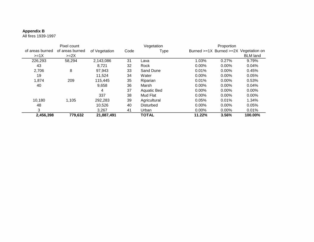
Appendix BAll fires 1939-1997

of areas burned >=1X

of areas burned >=2X

of Vegetation Code Type Burned >=1X Burned >=2X Vegetation on BLM land

ProportionVegetationPixel count

226,293 58,294 2,143,086 31 Lava 1.03% 0.27% 9.79%43 8,721 32 Rock 0.00% 0.00% 0.04%

2,706 8 97,943 33 Sand Dune 0.01% 0.00% 0.45%19 11,524 34 Water 0.00% 0.00% 0.05%

1,874 209 115,445 35 Riparian 0.01% 0.00% 0.53%40 9,658 36 Marsh 0.00% 0.00% 0.04%

4 37 Aquatic Bed 0.00% 0.00% 0.00%337 38 Mud Flat 0.00% 0.00% 0.00%

10,180 1,105 292,283 39 Agricultural 0.05% 0.01% 1.34%48 10,526 40 Disturbed 0.00% 0.00% 0.05%3 3,267 41 Urban 0.00% 0.00% 0.01%

2,456,398 779,632 21,887,491 TOTAL 11.22% 3.56% 100.00%

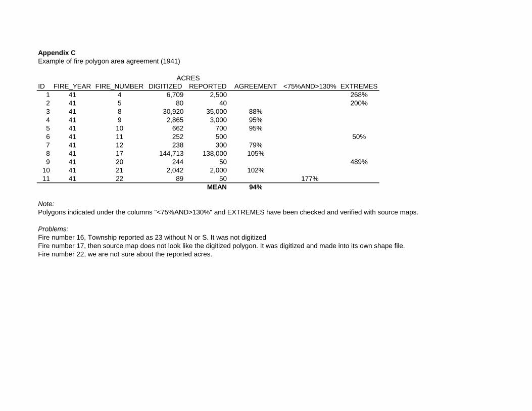
Appendix CExample of fire polygon area agreement (1941)

ID FIRE_YEAR FIRE_NUMBER DIGITIZED REPORTED AGREEMENT <75%AND>130% EXTREMES1 41 4 6,709 2,500 268%2 41 5 80 40 200%3 41 8 30,920 35,000 88%4 41 9 2,865 3,000 95%5 41 10 662 700 95%6 41 11 252 500 50%7 41 12 238 300 79%8 41 17 144,713 138,000 105%9 41 20 244 50 489%

10 41 21 2,042 2,000 102%11 41 22 89 50 177%

MEAN 94%

Note:Polygons indicated under the columns "<75%AND>130%" and EXTREMES have been checked and verified with source maps.

Problems:Fire number 16, Township reported as 23 without N or S. It was not digitizedFire number 17, then source map does not look like the digitized polygon. It was digitized and made into its own shape file.Fire number 22, we are not sure about the reported acres.

ACRES