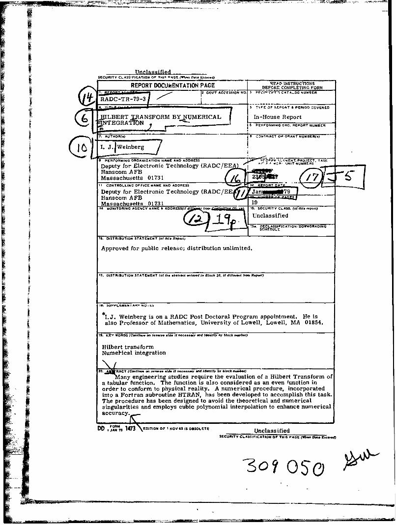
RADC-TR-79-3cX) In-House Report

January 1979

HILBERT TRANSFORM BYNUMERICAL INTEGRATIONI. J. Weinberg

ci_

-. J

LL.. APPROVIED FOR PUBLIC RELEASE; DISTRIBUTION UNLIMITEDj

DDC

ROME AIR DEVELOPMENT CENTERAir Force Systems CommandGriffiss Air Force Base, New York 13441

This report has been reviewed by thc RADC Information Office (01) and

is relcnsable to the National Technical Information Service (NTIS). At NTIS

it will be releasable to the general public, including foreign nations.

RADC-TR-79-3 has been reviewed and is approved for publication.

APPROVED): 4/A( Ak-0_WALTER ROTMANChief, Antennas & RF Components Branch

APPROVED:

A2 C. SCHELLChief, Electromagnetic Sciences Division

FOR THE COMMANDER:

6JOHN P. HUSSActing Chief, Plans Office

If your address has changed or if you wish to be removed from the RADCmailing list, or if the addressee is no longer employed by your organization,please notiry RADC (EEA), Hanscom AFB MA 01731. This will assist us inmaintaining a current mailing list.

Do not return this copy. Retain or destroy.

MISSIONof

Raw Air Developmnt Center

RADC plans and conducts research, exploratory and advanceddevelopment programs in command, conti'ol, and communications(C3) activities, and in the C3 areas of information sciencesand intelligence. The principal technical mission areasare conmiunications, electromagnetic guidance and control,

A surveillance ground and aerospace objects, Inrle..1data collection and handling, information system technology,ionospheric propagation, solid state sciences, microwavephysics and electronic reliability, maintainability andcompatibility.

Printed byUnited States Air ForceHanscom AFB, Mass. 01731

UnclasgiHiedSECURITY CLASSIFICATION OF TNII not 1P.. fl** c.-cd)

REPORT DOCUMENTATION PAGE EAD NSTUCTONS

TADC-TR-79-3 .

4 T% rE OF hPGAT A PERIOD COVERED

7. ATOTNR( PER"ORMING ORG. REPORT NUMBER

I. DECASIFIATON/OWORAIN

SEISTRIUTIORNIST ATIEN NAME AND ADRSSI -zAk ROET.)

Depprove for pletoic reease;g disrbution unIed

Hanscom _ __ _ __ __ _ __ _ __ _ __ __ _ __ _ __ _ __ _

Masahs.t DISRIBTIO STTMN o A bl.fmI. nBlc 0 Idloo, of7o

als ProfessorG ofNC NM&athemaics Unierit ofLoEI CLoelASS 01854.eprt

any engineeringN sTTMNT(ftis reqieteeautotf)etTasomo

Apptabulafr uti Thee; nc ibtion sauocnlidered.a nee ucini

orde DSRBTON conforMEN tof physcl ere ly. A0 numiferical protedueinororte

*into aeFortrn sboune H N as beenra devoedat aomplish Histak

Th. evOD produnreasbee sdei neayd Itof av o the thoretclad ueia

snulaiis n mposcuiolnmal interlaioaotnhnciumria

2'. mt ACT Cy. oor tosol*I oe-i n dnit yboc.tabt

any I niern stde require Ohe evauaio If OBaT UnclifedtTasomoa ~ ~ ~~ SCRT CLAaIFICTIr OFcton TNhe PAGEio is also cosierdasanevnfuctoni

order ~ ~ ~ ~ ~ ~ -to conor topyia7elt.Anmriarcdricroae

SECUMI7N CLASIFI~CATION OF TISg PA0E(tWhe, Oaf* gnfsfod)

SECURITY CLASSIFICATION OF THIS PAGErI7,. Uota EnI*,d)

WTI-

Preface

The author is grateful to James C. Sethares of RADC/EEA for valuable sug-gestions during the progress of the work.

IIT

0

3

Contents

1. INTRODUCTION 7

2. MATHEMATICAL ANALYSIS 8

3. NUMERICAL ANALYSIS 10

4. SUBROUTINE DESCRIPTION 13

5. PROGRAM LISTING 14

6. NUMERICAL EXAMPLES 156.1 Example 2 156.2 Example 2 156.3 Example 3 16

7. SUMMARY 17

REFEREINCE3 19

iii

ii

IIllustrations1. Values of the Independent and Dependent Variables Employed inj

the Numerical Integration Scheme I11

5

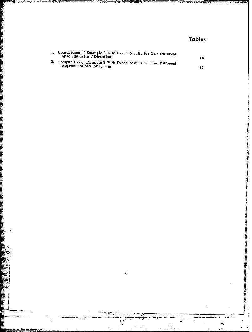
Tables

1. Comparison of Example 2 With Exact Results for Two DifferentSpacings in the f Direction 162. Comparison of Example 3 With Exact Results for Two Different

Approximations for f co 17

FN

6

-K

S5I

I _-

t Hilbert Transform by Numerical Integration

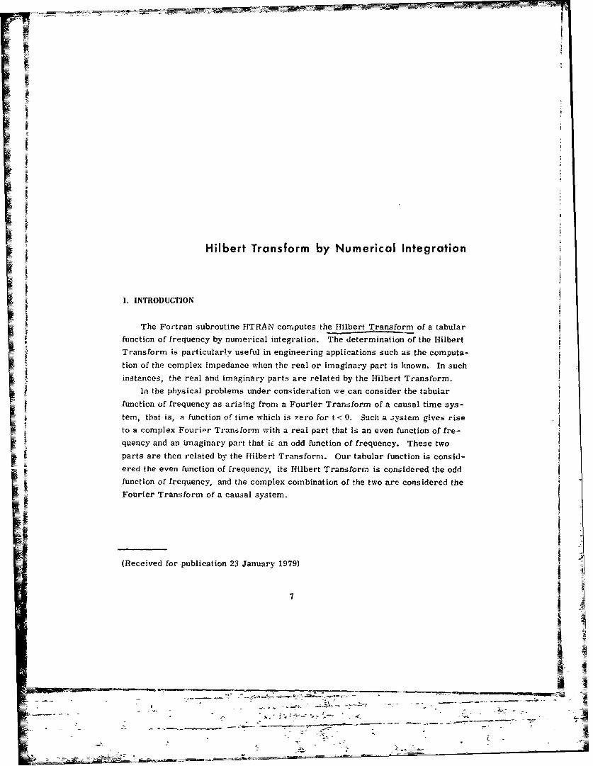
I. INTRODUCTION

The Fortran subroutine HTRAN computes the Hilbert Transform of a tabularfunction of frequency by numerical integration. The determination of the Hilbert

Transform is particularly useful in engineering applications such as the computa-

tion of the complex impedance when the real or imaginary part is known. In suchinstances, the real and imaginary parts are related by the Hilbert Transform.

In the physical problems under consideration we can consider the tabular

function of frequency as arising from a Fourier Transform of a causal time sys-

tern, that is, a function of time which is zero for t < 0. Such a .;zytem gives rise

to a complex Fouripr Transform with a real part that is an even function of fre-

quency and an imaginary part that it an odd function of frequency. These twoparts are then related by the Hilbert Transform. Our tabular function is consid-

I ered the even function of frequency, its Hilbert Transform is considered the oddIfunction of frequency, and the complex combination of the two are considered the

Fourier Transform of a causal system.

I1

-ii

I(Received for publication 23 January 1979) 21

7

iii_ _ _ _ _ _ _ _ _ _ _ _ _ _ _

V7 ME

2. MATHEMATICAL ANALYSIS

For a function of angular frequency, R(a,), the Hilbert Transform is defined

as

1 f (, dw ' . (1)X(W) d 0-

-CO

The integral is to be interpreted as the Cauchy Principal Value so that the singu-

larity arising in the denominator may be eliminated, that is

Co _c]

XI -lim R(W') do (t 2X()= lim___ +f dw (2)

When the given function is a function of frequency, R(f), we have

1f R(P) d 3Xlf) f f (3)

-00

which is interpreted as

Xl)=lira RIf) dHU+I~f)X(f) - - df' + df' (4)

fEf, fffA0 r+E

We seek to evaluate (3) when R(f) is in tabular form and is an even function of

frequency. It is also assumed that R(f) is described tabularly with equal spacing

in the frequency axis.

Since we will employ numerical Integration, we first modify expression (3)

in order to eliminate the singularity. We note, that

00

0 (5)fl-

-8o

II

in the sense of the Cauchy Principle Value since

l f d 'l- o d + f (6)C-,-+ f f 6

fJ~0

Thus any multiple of (5) may be added to (3). In particular, we may write

: - X(D = 1 HUI~f), -R(f) r 7

thus making the singularity in the integrand apparent. The integrand does notbecome arbitrarily large anywhere and is now suitable for "merical integration.

Since R(f) is an even function we have

R(-f) R(fl (8)

We assume R(f) to be zero outside the range of its tabular description. Denotingf as the first frequency and fN as the last frequency in the table we have

0 f<R( M 0 (9)

fN < f

We may now write (7) as

(-) R M,

X(R( df' + R( fdf' + j df'- t"gO-IN-f f-, - f

fN

f(10)' N 00f df' + f f'-f

- - f

9

7

iU

where our interest in f values is the range fl - f -< f Employing the evenness

property, we are able to obtain

2f Rf f (f') - R(f) df' + -R(f)X(f) i-7 f12-f2 df, + f f 2 d,+fF2f2dfu- fN

~(11)

The first and last integrals can be accomplished directly. Thus

X(f) R(f) In [ N( + 2ff (P) -R( df.. (12)f (f - fl1) f-N)

We are henceforth interested in the evaluation of the integral in (12), namely

fN

y(f) f R) - df' (13)fl

where the f values are in the range fl < f - fN"

3. NUMERICAL ANALYSIS

Although the integrand in (13) does not become arbitrarily large anywhere,

we are faced with an indeterminacy when f' equals f. The integration techniquei presently described has the feature that f' never attains any of the f values at

which Y is being calculated, thus avoiding the indeterminacy in the integrand.

Consider R(f) defined tabularly as pictured by the solid lines in Figure 1.

(fi' R i = 1, 2, . . ., N are given with the f values equally spaced. The subroutine

computes the Hilbert Transform at these same f values.

Now consider another set of f values, denoted by f, i 1, 2,..., N-1, each

of which is midway between two f values. Thus

fi+f~li 1 , 2,..N-1 (14)

2

as pictured by the broken lines in Figure 1. We first apply (12) to obtain the

Hilbert Transform, X, at these Tvalues where, in the numerical integration, f'

10

R (f)

21

itR2N-. 2 -

!; 2 12R RN-2

T I , T 1~

I II II

fl 7, f2 f2 f3 'N-2 IN-2 'N-1 'N-1 fN

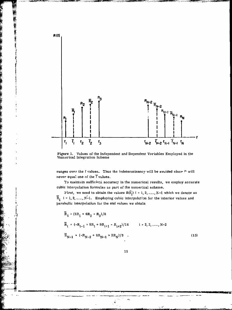
Figure 1. Values of the Independent and Dependent Vpriables Employed in theI Numerical Integration Scheme

ranges over the f values. Thus the indeterminancy will be avided since F' will

never equal one of the f values.To maintain sufficienL accuracy in the numerical results, we employ accurate

cubic interpolation formulas as part of the numerical scheme.

First, we need to obtain the values R(f.) i = 1, 2, ... , N-I which we denote as

paR i = 1, 2, N-1. Employing cubic interpolation for the interior values andparabolic interpolation for the end values we obtain

- i.R (3= 13 1 + 6R2 " R3)/8

R = (-RH 1 + 9R. + 9R 1 - Ri 2 )/16 i 2, 3, N-2

RNI = ( - RN -2 + 6RN-1 + 3RN)/3 (15)

11

We now write (13) as

N (P) R(f.

Yi = vy f -. 2 (f, i =1, 2,...N-1 (16)fi1 f f

which we write as, employing numerical integration,

Yii=1,2, .. ,N-I (17)

where, when N is odd, Simpson's Rule gives

hN h f/3

3h 46f/3 j 2,4,.. .,N-1 (j even) (18)

h. 26f/3 j =3, 5,. .N-2 (j odd)

and a~f is the spacing in the frequency axis.

When N is even the Trapezo-*dal Rule is used to include the last interval.

Thus

= Af/3

h. 46f /3 j2, 4, NI-2 (jeven)

h. =26f/3 j=3, 5, . ,N-3 (j odd) (19)

N-1

hN=Af/ 2

i ~ The Hilbert Transform at the f. i 1, 2, .. ., N-lI are obtained from (12) as

E]

12

: -- ---- = . . -- - - _ -- - -- - - - - - - -= =-----, -_ - - - ..... ..... - -.. . .

To obtain the Hilbert Transform, X., at the f. i = 1, 2, .... N we again per-

form an accurate interpolation; cubic interpolation for the interior values and

parabolic interpolat,*on for two values at each end. Thus

xi (15X 1 - 10X 2 + 3X 3)/8

2 (3X 1 + 6X 2 -3

X - (-i- 2 + 9 -+ 5 l ) / 1 6 i = 3,4, .. , N-2 (21)

XN-l = (-XN-3 + 6 XN- 2 + 3X N-I)/8

XN = (3ON- 3 - loXN- 2 + 15XN-1)/8

We thus obtain the tabular results (fi, X1' i = 1, 2, ... , N as the Hilbert

Transform values for the given (fi. Ri) i 1, 2, .... , N. The only assumption

made concerning the function R(f) is that it is an even function of frequency,

complying with phys' al reality. It is also assumed that the function R(f) is

described tabularly with equal spacLng in f. To insure sufficient accuracy in the

numerical integrations and interpolations, one should make the frequency interval

adequately small or, correspondingly, N sufficiently large.

4. SUBROUTINE DESCRIPTION

The user employs the Hilbert Transforms subroutine HTRAN by the state-

ment

CALL HTRAN (R, X, N, FBEG, FEND)

The arguments in the subroutine are described as follows:

R - a dimensioned array containing the tabular values of R.

X - a dimensioned a-ray containing the Hilbert Transform values of Xreturned by the subroutine HTRAN.

N - the number of values contained in the table of 1R (and X).

FBEG - the first frequency, fl. for the H array.

FEND - the last frequency, fN' for the R array.

Since equal spacing in the frequency axis is assumed, the items N, FBEG

and FEND permit the subroutine to determine the values fi i 1, 2,..., N.

13

•I

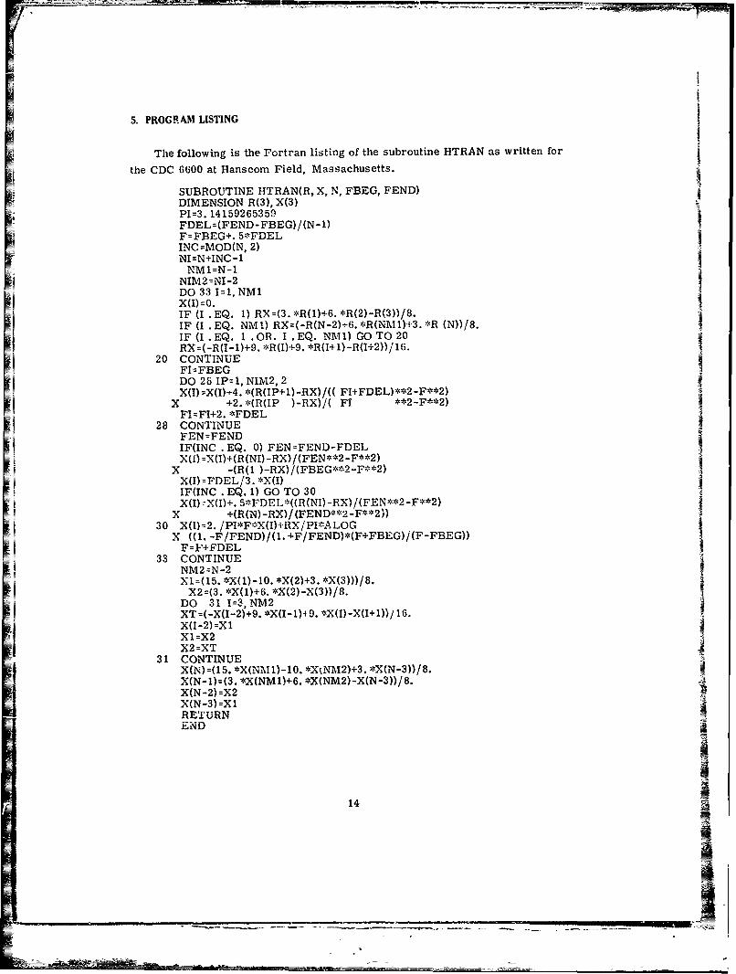
5. PROGRPAM LISTING

The following is the Fortran listing of the subroutine HTRAN as written for

the CDC 6600 at Hanscom Field, Massachusetts.

SUBROUTINE HTRAN(R, X, N, FEEG, FEND)DIMENSION R(3), X(3)PI=3. 14159265359FDEL=(FEND-FBEG)/(N-l)IF=FBEG+. 5*FDELINC =MOD(N, 2)NI=N+INC -1

NM1=N-1NIM2 'NI-2DO 33 1=1, NMIX(I)=0.IF (I .EQ. 1) RX =(3. *R(1)+6. *R(2)-R(3))/8.IF (I .EQ. NMI) RX=(-R(N-2)-±6. *R(NM1)±3. *fl (N))/8.IF (I .EQ. 1 .OR. I .EQ. NMI1) GO TO 20RX=(-R(I-l)+9. *R(I)+9. *R(141)-R(1+2))/16.

20 CONTINUEFI=FBEGDO 28 IP=l1, NIM2, 2

X(I) I)--4. (R(P+I-RX) FI+DEL)*2-**2

X +2. *(R(IP )-RX)( F1 **2-F**2)FI=FI+2. *FDEL

28 CONTINUEFEN =FENDIF(INC .EQ. 0) FEN=FEND-FDEL

X(I) =X(I)+(R(NI) -RX)/(FEN**2 -F**2)x-(R(i )-RX)/(FBEG**2..F**2)

IF(INC . EQ. 1) GO TO 30X(I) =X(I)+. S*FDEL*((R (NI) -RX) /(FEN **2 -F**2)

x+(R(N)-RX)/(FEND**2-F**2,)30 X(1)=2. /PI*F*X(I)+RX/ PI*A LOG

X ((1. -F /FEND)/ (1. +F/ FEND) *(F+FBEG)j(F -FBEG))33 1DE33CONTINUE

NM2=N-2

DO 31 1=3, NM2XT =(-X(I-2)+9. *X(I- 1)49. *X(I) -X(I+1))/ 16.X(I-2)=Xl XI=X2

X2=XT31 CONTINUE

X(N-0)=(. *X(,NA41)46. *X(NM2)-X(N-3))/ 8.X(N -2) =X2X(N-3) =X1RETURNEND

14

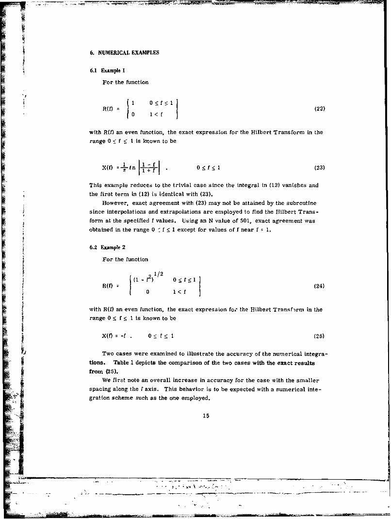
6. NUMERICAL EXAMPLES

6.1 Example I

For the function

S1 0 f< 1

R(f) - (22)0 1< f

with R(f) an even function, the exact expression for the Hilbert Transform in the

range 0 < f :g 1 is known to be

X(f) I n f 01fI 1 (23)

This example reduces to the trivial case since the integral in (12) vanishes and

the first term in (12) is identical with (23).

However, exact agreement with (23) may not be attained by the subroutinesince interpolations and extrapolations are employed to find the Hilbert Trans-

form at the specified f values. Using an N value of 501, exact agreement was

obtained in the range 0 f 1 except for values of f near f =1.

6.2 Example 2

For the function

(1-f 2) 0<f<lR(f) (24)

0 1< f

t with R(f) an even function, the exact expression foi the Hilbert Transf-,rm in the

range 0 _ f_ I is known to be

X(f) -f 0 f 1 (25)

Two cases were examined to illustrate the accuracy of the numerical integra-

tions. Table 1 depicts the comparison of the two cases with the exact results

from (25).We first note an overall increase in accuracy for the case with the smaller

j spacing along the f axis. This behavior is to be expected with a numerical inte-gration scheme auch as the one employed.

15

Table 1. Comparison of Example 2 With Exact Results for Two

Different Spacirgs in the f Direction

f exact f .005 f .002

-1 0 1 1 2

0 0 -. 9395268 X 10-10 2351980 X 10-

0.1 -. 1 -. 1000026 -. 1000007

0.2 -.2 -.2000054 -.2000014

0.3 -.3 -.3000085 -.3000022

0.4 -.4 -.4000123 -.4000031

0. 5 -. 5 -. 5000172 -. 5000044

0.6 -.6 -.6000242 -.6000061

0.7 -.7 -.7000354 -.7000090

0.8 -.8 -. 8000572 -.8000145

0.9 -. 9 -.9001214 -.9000309

1.0 -1.0 -1. 014396 -1. 009106

We also note a decrease in accuracy in both cases as f increases from 0 to 1.

This may be explained by the nature of the R(f) function (24). The magnitude of

the slope of R(f), and consequently also for the integrand in (12), increasesgreatly as f goes from 0 to 1. This could well affect the accuracy of the numer-

ical integrations.

6.3 Example 3

For the function

R(f) in f (26)2 7r f

with R(f) an even function, the exact expression for the Hilbert Transform valid

in the range 0 f is known to be

X( cos 2f-1 0 < f (27)

Two cases were examined here to illustrate the effect of the numerical

approximation for oo. In one case the upper limit of f, fN' was chosen as 10 with

an N of 641 making a spacing Af = 1/64. In the second case fN was chosen as 20with an N of 1281 thus keeping the same spacing Af = 1/64. Table 2 shows the

comparison of the two cases with exact results (27) for the upper limit of f being 00.R

163

M..A-

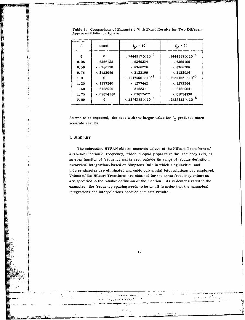
Table 2. Comparison of Example 3 With Exact Results for Two DifferentApproximations for fN CO

f exact fN 0N fN 20..0 0 .7444819 X 10 4 .7444819 X 10 4

0.25 -.6366198 -.6366234 -.6366199

0.50 -.6366198 -.6366276 -.6366206

0.75 -.2122066 -.2122190 -.2122084

1.0 0 -,1647500 X 10 4 .2255452 X 10 5

1.25 -.1273240 -.1273442 -.1273264

1.50 -.2122066 -.2122311 -.2122094

1.75 -.09094568 -.09097477 -.09094930

2.00 0 -. 3364389 X 10-4 .4225282 X 10-5

As was to be expected, the case with the larger value for fN produces more

accurate results.

7. SUMMARY

The subroutine UTRAN obtains accurate values of the Hilbert Transform of

a tabular function of frequency, which is equally spaced in the frequency axis, is

an even function of frequency and is zero outside its range of tabular definition.

Numerical integrations based on Simpsons Rule in which singularities and

indeterminacies are eliminated and cubic polynomial interpolations are employed.

Values of the Hilbert Transform are obtained for the same frequency values as

are specified in the tabular definition of the function. As is demonstrated in the

examples, the frequency spacing needs to be small in order that the numerical

integrations and interpolations produce accurate results.

17° A

References

1. Bateman Manuscript Project (1954) Table of Integral Transforms, McGr'aw-Hill.

2. Papoulis, A. (1962) The Fourier Integral and its A pplications, McGraw-Hill.

'3. Ganguly, A. K., Webb, D.C., and Banks, C. (1078) Complex RadiationImpedance of Microstrip-Excited Magnetottte-aeWa-ves. lltlHE,Transactions on Microwave Theory and 'Tcchniques, pp, 444-447.

4. Wu, I.J. (1077) Ph. D. Thesis, University of Texas at Arlington, Dcpartmentof Electrical Engineering.

10