
Highway Hierarchies Star - KIT - ITI Algorithmik
34
DIMACS Series in Discrete Mathematics and Theoretical Computer Science Highway Hierarchies Star Daniel Delling, Peter Sanders, Dominik Schultes, and Dorothea Wagner Abstract. We study two speedup techniques for route planning in road net- works: highway hierarchies (HH) and goal directed search using landmarks (ALT). It turns out that there are several interesting synergies. Highway hi- erarchies yield a way to implement landmark selection more efficiently and to store landmark information more space efficiently than before. ALT gives queries in highway hierarchies an excellent sense of direction and allows some pruning of the search space. For computing shortest distances and approxi- mately shortest travel times, this combination yields significant speedups (be- tween a factor of 2.5 and 5) over HH alone, while for exact queries using the travel time metric only minor improvements are achieved. We also explain how to compute actual shortest paths very efficiently. 1. Introduction Computing fastest routes in a road networks G =(V,E) from a source s to a target t is one of the showpieces of real-world applications of algorithmics. In principle, we could use Dijkstra’s algorithm [3]. But for large road networks this would be far too slow. Therefore, there is considerable interest in speedup techniques for route planning. A classical technique that gives a speedup of around two for road networks is bidirectional search which simultaneously searches forward from s and backwards from t until the search frontiers meet. Most speedup techniques use bidirectional search as an (optional) ingredient. Another classical approach is goal direction via A ∗ search [9]: lower bounds define a vertex potential that directs the search towards the target. This approach was recently shown to be very effective if lower bounds are computed using pre- computed shortest path distances to a carefully selected set of about 20 Landmark nodes [5, 7] using the Triangle inequality (ALT ). Speedups up to a factor 30 over bidirectional Dijkstra can be observed. A property of road networks worth exploiting is their inherent hierarchy. Com- mercial systems use information on road categories to speed up search. ‘Sufficiently 2000 Mathematics Subject Classification. Primary 68R10; Secondary 90B20. Key words and phrases. Shortest paths, graph, speed-up technique, hierarchy, goal-direction, preprocessing, routing, road network. Partially supported by DFG grant SA 933/1-3. and by the Future and Emerging Technologies Unit of EC (IST priority – 6th FP), under contract no. FP6-021235-2 (project ARRIVAL). c 2008 American Mathematical Society 1
Transcript of Highway Hierarchies Star - KIT - ITI Algorithmik
DIMACS Series in Discrete Mathematics
and Theoretical Computer Science
Highway Hierarchies Star
Daniel Delling, Peter Sanders, Dominik Schultes, and Dorothea Wagner
Abstract. We study two speedup techniques for route planning in road net-works: highway hierarchies (HH) and goal directed search using landmarks(ALT). It turns out that there are several interesting synergies. Highway hi-erarchies yield a way to implement landmark selection more efficiently andto store landmark information more space efficiently than before. ALT givesqueries in highway hierarchies an excellent sense of direction and allows somepruning of the search space. For computing shortest distances and approxi-mately shortest travel times, this combination yields significant speedups (be-tween a factor of 2.5 and 5) over HH alone, while for exact queries using thetravel time metric only minor improvements are achieved. We also explainhow to compute actual shortest paths very efficiently.
1. Introduction
Computing fastest routes in a road networks G = (V, E) from a source s toa target t is one of the showpieces of real-world applications of algorithmics. Inprinciple, we could use Dijkstra’s algorithm [3]. But for large road networksthis would be far too slow. Therefore, there is considerable interest in speeduptechniques for route planning.
A classical technique that gives a speedup of around two for road networks isbidirectional search which simultaneously searches forward from s and backwardsfrom t until the search frontiers meet. Most speedup techniques use bidirectionalsearch as an (optional) ingredient.
Another classical approach is goal direction via A∗ search [9]: lower boundsdefine a vertex potential that directs the search towards the target. This approachwas recently shown to be very effective if lower bounds are computed using pre-computed shortest path distances to a carefully selected set of about 20 Landmarknodes [5, 7] using the Triangle inequality (ALT ). Speedups up to a factor 30 overbidirectional Dijkstra can be observed.
A property of road networks worth exploiting is their inherent hierarchy. Com-mercial systems use information on road categories to speed up search. ‘Sufficiently
2000 Mathematics Subject Classification. Primary 68R10; Secondary 90B20.Key words and phrases. Shortest paths, graph, speed-up technique, hierarchy, goal-direction,
preprocessing, routing, road network.Partially supported by DFG grant SA 933/1-3. and by the Future and Emerging Technologies
Unit of EC (IST priority – 6th FP), under contract no. FP6-021235-2 (project ARRIVAL).
c©2008 American Mathematical Society
1
2 D. DELLING, P. SANDERS, D. SCHULTES, AND D. WAGNER
far away’ from source and target, only ‘important’ roads are used. This requiresmanual tuning of the data and a delicate tradeoff between computation speed andsuboptimality of the computed routes. In a previous paper [16] we introducedthe idea to automatically compute highway hierarchies that yield optimal routesuncompromisingly quickly. This was the first speedup technique that was ableto preprocess the road network of a continent in realistic time and obtain largespeedups (several thousands) over Dijkstra’s algorithm. In [17] the basic methodwas considerably accelerated using many small measures and using distance tables :shortest path distances in the highest level of the hierarchy are precomputed. Thisway, it suffices to search locally around source and target node until the shortestpath distance can be found by accessing the distance table.
A different hierarchy-based method—reach-based routing [8]—profits consid-erably from a combination with ALT [4]. The present state of affairs is that thecombined method from [4] shows performance somewhat inferior to highway hier-archies with distance tables but without goal direction. Both methods turn out tobe closely related. In particular, [4] uses methods originally developed for highwayhierarchies to achieve fast preprocessing. Here, we explore the natural questionhow highway hierarchies can be combined with goal directed search in general andwith ALT in particular.
1.1. Overview and Contributions. In the following sections we first reviewhighway hierarchies in Section 2 (Algorithm HH) [17]. A new result presented thereis a very fast algorithm for explicitly computing the shortest paths by precomputingunpacked versions of shortcut edges. Section 3 reviews Algorithm ALT [5, 7] andintroduces refined algorithms for selecting landmarks. The main innovation thereis restricting landmark selection to nodes on higher levels of the highway hierarchy.
The actual integration of highway hierarchies with ALT (Algorithm HH∗) is in-troduced in Section 4. This is nontrivial in several respects. For example, we needincremental access to the distance tables for finding upper bounds and a differentway to control the progress of forward and backward search. We also have to over-come the problem that search cannot be stopped when search frontiers meet. Onthe other hand, there are several simplifications compared to ALT. Abandoning thereliance on a stopping criterion allows us to use simpler, faster, and stronger lowerbounds. Using distance tables obviates the need for dynamic landmark selection.Another interesting approach is to stop the search when a certain guaranteed solu-tion quality has been obtained. There are several interesting further optimisations.In particular, we can be more space efficient than ALT by storing no landmarkinformation on the lowest level of the hierarchy. We describe how the missing infor-mation can be reconstructed efficiently at query time. As a side effect, we introducea way to limit the length of shortcuts. This measure turns out to be of independentinterest since it also improves the basic HH algorithm. Note that Goldberg et al.[6] use similar techniques as we do in order to reduce the memory consumptionof landmarks when combined with reach-based routing. They have already brieflymentioned this idea in [4].
Section 5 reports extensive experiments performed using road networks of West-ern Europe and the USA. Section 6 summarises the results and outlines possiblefuture work.
HIGHWAY HIERARCHIES STAR 3
1.2. More Related Work. There are several other approaches to goal di-rected search. Our first candidate for combination with highway hierarchies werePrecomputed Cluster Distances [12]. PCDs allow the computation of upper andlower bounds based on precomputed distances between partitions of the road net-works. These lower bounds cannot be used for A∗ search since they can producenegative reduced edge weights so that Dijkstra’s algorithm is no longer applica-ble. The search space can still be pruned by discontinuing search at node v if thelower bound from v to t indicates that the best upper bound seen so far cannotpossibly be improved when passing through v. An advantage of PCDs over land-marks is that they need less space. We did not implement this however since PCDsare rather ineffective for search in the lower levels of the hierarchy and since ourdistance table optimisation from [17] is already very effective for pruning search atthe higher levels of the hierarchy. In contrast, landmarks can be used together withA∗ search and thus can direct the search towards the target already in the lowerlevels of the hierarchy.
An important family of speedup techniques [20, 13, 11] associates informationwith each edge e. This information specifies a superset of the nodes reached viae on some shortest path. Geometric containers [20] require node coordinates andstore a simple geometrical object containing all the nodes reached via a shortestpath. Edge flags partition the graph into regions. For each edge e and each regionR one bit specifies whether there is a shortest path via e into region R [13, 11].Both techniques alone already contain both direction information and hierarchyinformation so that very big speedups, comparable to highway hierarchies, can beachieved. However, so far these methods would have forbiddingly large prepro-cessing times for the largest available road networks. Therefore these approacheslooked not so interesting for a first attempt to combine goal directed search withhighway hierarchies.
2. Highway Hierarchies
The basic idea of the highway hierarchies approach is that outside some localareas around the source and the target node, only a subset of ‘important’ edgeshas to be considered in order to be able to find the shortest path. The concept ofa local area is formalised by the definition of a neighbourhood node set1 N(v) foreach node v. Then, the definition of a highway network of a graph G = (V, E) thathas the property that all shortest paths are preserved is straightforward: an edge(u, v) ∈ E belongs to the highway network iff there are nodes s, t ∈ V such thatthe edge (u, v) appears in the canonical shortest path2 〈s, . . . , u, v, . . . , t〉 from s tot in G with the property that v 6∈ N(s) and u 6∈ N(t).
The size of a highway network (in terms of the number of nodes) can be consid-erably reduced by a contraction procedure: for each node v, we check a bypassabilitycriterion that decides whether v should be bypassed—a operation that removes thenode and creates shortcut edges (u, w) representing paths of the form 〈u, v, w〉. The
1In [17], we give more details on the definition of neighbourhoods. In particular, we distin-guish between a forward and a backward neighbourhood. However, in this context, we would liketo slightly simplify the notation and concentrate on the concepts that are important to understandthe subsequent sections. The implementation, however, is based on [17] and not simplified.
2For each connected node pair (s, t), we select a unique canonical shortest path in such a waythat each subpath of a canonical shortest path is canonical as well. For details, we refer to [16].
4 D. DELLING, P. SANDERS, D. SCHULTES, AND D. WAGNER
graph that is induced by the remaining nodes and enriched by the shortcut edgesforms the core of the highway network. The bypassability criterion takes into ac-count the degree of the node v and the number of shortcuts that would be created ifv was bypassed: the net increase of the number of edges due to a bypass operationshould be small. For details, we refer to [17].
A highway hierarchy of a graph G consists of several levels G0, G1, G2, . . . , GL.Level 0 corresponds to the original graph G. Level 1 is obtained by computing thehighway network of level 0, level 2 by computing the highway network of the coreof level 1 and so on.
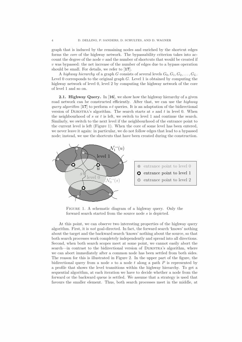
2.1. Highway Query. In [16], we show how the highway hierarchy of a givenroad network can be constructed efficiently. After that, we can use the highwayquery algorithm [17] to perform s-t queries. It is an adaptation of the bidirectionalversion of Dijkstra’s algorithm. The search starts at s and t in level 0. Whenthe neighbourhood of s or t is left, we switch to level 1 and continue the search.Similarly, we switch to the next level if the neighbourhood of the entrance point tothe current level is left (Figure 1). When the core of some level has been entered,we never leave it again: in particular, we do not follow edges that lead to a bypassednode; instead, we use the shortcuts that have been created during the construction.
N→
1 (u)
level 1
level 0N→
0 (s)
entrance point to level 1u
entrance point to level 2
entrance point to level 0
s
Figure 1. A schematic diagram of a highway query. Only theforward search started from the source node s is depicted.
At this point, we can observe two interesting properties of the highway queryalgorithm. First, it is not goal-directed. In fact, the forward search ‘knows’ nothingabout the target and the backward search ‘knows’ nothing about the source, so thatboth search processes work completely independently and spread into all directions.Second, when both search scopes meet at some point, we cannot easily abort thesearch—in contrast to the bidirectional version of Dijkstra’s algorithm, wherewe can abort immediately after a common node has been settled from both sides.The reason for this is illustrated in Figure 2. In the upper part of the figure, thebidirectional query from a node s to a node t along a path P is represented bya profile that shows the level transitions within the highway hierarchy. To get asequential algorithm, at each iteration we have to decide whether a node from theforward or the backward queue is settled. We assume that a strategy is used thatfavours the smaller element. Thus, both search processes meet in the middle, at

HIGHWAY HIERARCHIES STAR 5
s
P
a
t
c
b
s
Q
Level 2
Level 1
Level 0
Level 2
Level 1
Level 0t
Figure 2. Schematic profile of a bidirectional highway query.
node a. When this happens, a path from s to t has been found. However, wehave no guarantee that it is the shortest one. In fact, the lower part of the figurecontains the profile of a shorter path Q from s to t, which is less symmetric than theprofile of P . Note that the very flexible definition of the neighbourhoods allows suchasymmetric profiles. When a on P is settled from both sides, b has been reachedon Q by the backwards search, but not by the forward search since a search processnever goes downwards in the hierarchy: therefore, at node c, the forward search isnot continued on the path Q. We find the shorter path Q not until the backwardsearch has reached c—which happens after P has been found. Hence, it would bewrong to abort the search when a has been settled.
In [16], we introduced some rather complicated abort criteria, which we droppedin [17] since they did reduce the search space, but the evaluation of the criteriawas too expensive. Instead, we use a very simple criterion: the forward (backward)search is not continued if the key of the minimum element of the forward (back-ward) queue is larger then the current upper bound (i.e., the length of the tentativeshortest path).
2.2. Using a Distance Table. The construction of fewer levels of the high-way hierarchy and the usage of a complete distance table for the core of the top-most level can considerably accelerate the query: whenever the forward (backward)search enters the core of the topmost level at some node u, u is added to a node
set−→I (←−I ) and the search is not continued from u. Since all distances between
the nodes in the sets−→I and
←−I have been precomputed and stored in a table,
we can easily determine the shortest path length by considering all node pairs
(u, v), u ∈−→I , v ∈
←−I , and summing up d(s, u) + d(u, v) + d(v, t). For details, we
refer to [17].Using the distance table can be seen as extreme case of goal-directed search:
from the nodes in the set−→I , we directly ‘jump’ to the nodes in the set
←−I , which
are close to the target. Thus, we can say that the highway query with the distancetable optimisation works in two phases: a strictly non-goal-directed phase till the
sets−→I and
←−I have been determined, followed by a ‘goal-directed jump’ using the
distance table.
2.3. Complete Description of the Shortest Path. So far, we have dealtonly with the computation of shortest path distances. In order to determine acomplete description of the shortest path, we have to a) bridge the gap between
6 D. DELLING, P. SANDERS, D. SCHULTES, AND D. WAGNER
the forward and backward topmost-core entrance points and b) expand the usedshortcuts to obtain the corresponding subpaths in the original graph.
Problem a) can be solved using a simple algorithm: We start with the forwardcore entrance point u. As long as the backward entrance point v has not beenreached, we consider all outgoing edges (u, w) in the topmost core and check whetherd(u, w) + d(w, v) = d(u, v); we pick an edge (u, w) that fulfils the equation, and weset u := w. The check can be performed using the distance table. It allows us togreedily determine the next hop that leads to the the backward entrance point.
Problem b) can be solved without using any extra data (Variant 1): for eachshortcut (u, v), we perform a search from u to v in order to determine the path inthe original graph; this search can be accelerated by using the knowledge that thefirst edge of the path enters a component C of bypassed nodes, the last edge leadsto v, and all other edges are situated within the component C.
However, if a fast output routine is required, it is necessary to spend someadditional space to accelerate the unpacking process. We use a rather sophisticateddata structure to represent unpacking information for the shortcuts in a space-efficient way (Variant 2). In particular, we do not store a sequence of node IDs thatdescribe a path that corresponds to a shortcut, but we store only hop indices : foreach edge (u, v) on the path that should be represented, we store its rank withinthe ordered group of edges that leave u. Since in most cases the degree of a nodeis very small, these hop indices can be stored using only a few bits (in a fixed-length encoding). The unpacked shortcuts are stored in a recursive way, e.g., thedescription of a level-2 shortcut may contain several level-1 shortcuts. Accordingly,the unpacking procedure works recursively.
To obtain a further speed-up, we have a variant of the unpacking data struc-tures (Variant 3) that caches the complete descriptions—without recursions—of allshortcuts that belong to the topmost level, i.e., for these important shortcuts thatare frequently used, we do not have to use a recursive unpacking procedure, but wecan just append the corresponding subpath to the resulting path.
3. A∗ Search Using Landmarks
In this section we explain the known technique of A∗ search [9] in combinationwith landmarks. We follow the implementation presented in [7]. In Section 3.2we introduce a new landmark selection technique called advancedAvoid. Further-more, we present how the selection of landmarks can be accelerated using highwayhierarchies.
The search space of Dijkstra’s algorithm can be visualised as a circle aroundthe source. The idea of goal-directed or A∗ search is to push the search towardsthe target. By adding a potential π : V → R to the priority of each node, the orderin which nodes are removed from the priority queue is altered. A ‘good’ potentiallowers the priority of nodes that lie on a shortest path to the target. It is easy tosee that A∗ is equivalent to Dijkstra’s algorithm on a graph with reduced costs,formally wπ(u, v) = w(u, v)− π(u) + π(v). Since Dijkstra’s algorithm works onlyon nonnegative edge costs, not all potentials are allowed. We call a potential πfeasible if wπ(u, v) ≥ 0 for all (u, v) ∈ E. The distance from each node v of G tothe target t is the distance from v to t in the graph with reduced edge costs minusthe potential of t plus the potential of v. So, if the potential π(t) of the target t iszero, π(v) provides a lower bound for the distance from v to the target t.
HIGHWAY HIERARCHIES STAR 7
Bidirectional A∗. At first glance, combining A∗ and bidirectional search seemseasy. Simply use a feasible potential πf for the forward and a feasible potential πr
for the backward search. However, such an approach does not work due to the factthat the searches might work on different reduced costs, so that the shortest pathmight not have been found when both searches meet. This can only be guaranteed ifπf and πr are consistent, meaning wπf
(u, v) in G is equal to wπr(v, u) in the reverse
graph. We use the variant of an average potential function [10] defined as pf (v) =(πf (v) − πr(v))/2 for the forward and pr(v) = (πr(v) − πf (v))/2 = −pf(v) for thebackward search. By adding πr(t)/2 to the forward and πf (s)/2 to the backwardsearch, pf and pr provide lower bounds to the target and source, respectively. Notethat these potentials are feasible and consistent but provide worse lower boundsthan the original ones.
ALT.. There exist several techniques [18, 21] to obtain feasible potentialsusing the layout of a graph. The ALT algorithm uses a small number of nodes—socalled landmarks—and the triangle inequality to compute feasible potentials. Givena set S ⊆ V of landmarks and distances d(L, v), d(v, L) for all nodes v ∈ V andlandmarks L ∈ S, the following triangle inequalities hold:
d(u, v) + d(v, L) ≥ d(u, L) and d(L, u) + d(u, v) ≥ d(L, v)
Therefore, d(u, v) := maxL∈S max{d(u, L) − d(v, L), d(L, v) − d(L, u)} provides afeasible lower bound for the distance d(u, v). The quality of the lower bounds highlydepends on the quality of the selected landmarks.
Our implementation uses the tuning techniques of active landmarks, pruningand the enhanced stopping criterion. We stop the search if the sum of minimumkeys in the forward and the backward queue exceed µ + pf(s), where µ representsthe tentative shortest path length and is therefore an upper bound for the shortestpath length from s to t. For each s-t query only two landmarks—one ‘before’ thesource and one ‘behind’ the target—are initially used. At certain checkpoints wedecide whether to add an additional landmark to the active set, with a maximalamount of six landmarks. Pruning means that before relaxing an arc (u, v) duringthe forward search we also check whether d(s, u) + w(u, v) + πf (v) < µ holds. Thistechnique may be applied to the backward search easily. Note that for pruning, thepotential function need not be consistent.
3.1. Landmark Selection. A crucial point in the success of a high speedupwhen using ALT is the quality of landmarks. Since finding good landmarks is hard,several heuristics [5, 7] exist. We focus on the best known techniques; avoid andmaxCover.
Avoid. This heuristic tries to identify regions of the graph that are not wellcovered by the current landmark set S. Therefore, a shortest-path tree Tr is grownfrom a random node r. The weight of each node v is the difference between d(v, r)and the lower bound d(v, r) obtained by the given landmarks. The size of a node vis defined by the sum of its weight and the size of its children in Tr. If the subtreeof Tr rooted at v contains a landmark, the size of v is set to zero. Starting fromthe node with maximum size, Tr is traversed following the child with highest size.The leaf obtained by this traversal is added to S. In this strategy, the first rootis picked uniformly at random. The following roots are picked with a probabilityproportional to the square of the distance to its nearest landmark.

8 D. DELLING, P. SANDERS, D. SCHULTES, AND D. WAGNER
MaxCover [7]. The main disadvantage of avoid is the starting phase of theheuristic. The first root is picked at random and the following landmarks arehighly dependent on the starting landmark. MaxCover improves on this by firstchoosing a candidate set of landmarks (using avoid) that is about four times largerthan needed. The landmarks actually used are selected from the candidates usingseveral attempts with a local search routine. Each attempt starts with a randominitial selection.
3.2. New Selection Techniques. In the following we introduce a new heuris-tic called advancedAvoid to select landmarks. Furthermore, we use the highwayhierarchies to speed up the selection of landmarks.
AdvancedAvoid. Another approach to remedy for the disadvantages of avoid isto exchange the first landmarks generated by the avoid heuristic. More precisely,we generate k avoid landmarks, then take the first k′ landmarks from the set S andgenerate k′ new landmarks using avoid again. The advantage of advancedAvoidcompared to maxCover is the computation time. While maxCover takes about fivetimes longer than avoid, the selection of 16 advancedAvoid (k′ = 6) landmarks onthe road network of Western Europe takes about 45% more time than pure avoid.
Core Landmarks. The computation of landmarks is expensive. CalculatingmaxCover landmarks on the European network takes about 75 minutes, while con-structing the whole highway hierarchy can be done in about 15 minutes. A promis-ing approach is to use the highway hierarchy to reduce the number of possiblelandmarks: The level-1 core of the European road network has six times fewer
Figure 3. 16 advancedAvoid core 1 landmarks on the WesternEuropean road network
HIGHWAY HIERARCHIES STAR 9
nodes than the original network and its construction takes only about three min-utes. Using this level-1 core as possible positions for landmarks, the computationtime for calculating landmarks (all heuristics) can be decreased. Note that usingthe nodes of higher level cores reduces the time for selecting landmarks even more.However, the core of a highway hierarchy shrinks towards the centre of the mapand in [5], it has already been observed that good landmarks lie on the edge of amap (see Figure 3 for an example). Hence, using cores of a too high level wouldprobably yield worse landmarks.
4. Combining Highway Hierarchies and A∗ Search
Previously (see Section 2), we strictly separated the search phase to the topmost
core from the access to the distance table: first, the sets of entrance points−→I and
←−I into the core of the topmost level were determined, and afterwards the tablelook-ups were performed. Now we interweave both phases: whenever a forward
topmost-core entrance point u is discovered, it is added to−→I and we immediately
consider all pairs (u, v), v ∈←−I , in order to check whether the tentative shortest path
length µ can be improved. (An analogous procedure applies to the discovery of abackward core entrance point.) This new approach is advantageous since we can usethe tentative shortest path length µ as an upper bound on the actual shortest pathlength. In [16, 17], the highway query algorithm used a strategy that compares theminimum elements of both priority queues and prefers the smaller one in order toserialise forward and backward search. If we want to obtain good upper bounds veryfast, this might not be the best choice. For example, if the source node belongs toa densely populated area and the target to a sparsely populated area, the distancesfrom the source and target to the entrance points into the core of the topmost level
will be very different. Therefore, we now choose a strategy that balances |−→I | and
|←−I |, preferring the direction that has encountered fewer entrance points. In case
of equality (in particular, in the beginning when |−→I | = |
←−I | = 0), we use a simple
alternating strategy.We enhance the highway query algorithm with goal-directed capabilities—
obtaining an algorithm that we call HH∗ search—by replacing edge weights byreduced costs using potential functions πf and πr for forward and backward search.By this means, the search is directed towards the respective target, i.e., we arelikely to find some s-t path very soon. However, just using the reduced costs onlychanges the order in which the nodes are settled, it does not reduce the searchspace. The ideal way to benefit from the early encounter of the forward and back-ward search would be to abort the search as soon as an s-t path has been found.And, as a matter of fact, in the case of the ALT algorithm [5]—even in combi-nation with reach-based routing [4]—it can be shown that an immediate abort ispossible without losing correctness if consistent potential functions are used (seeSection 3). In contrast, this does not apply to the highway query algorithm sinceeven in the non-goal-directed variant of the algorithm, we cannot abort when bothsearch scopes have met (see Section 2).
Fortunately, there is another aspect of goal-directed search that can be ex-ploited, namely pruning: finding any s-t path also means finding an upper bound µon the length of the shortest s-t path. Comparing the lower bounds with the upperbound can be used to prune the search. In Section 3, the pruning of edges has

10 D. DELLING, P. SANDERS, D. SCHULTES, AND D. WAGNER
already been mentioned. Alternatively, we can prune nodes : if the key of a settlednode u is greater than the upper bound, we do not have to relax u’s edges. Notethat, using reduced costs, the key of u is the distance from the corresponding sourceto u plus the lower bound on the distance from u to the corresponding target.
Since we do not abort when both search scopes have met and because we havethe distance table, a very simple implementation of the ALT algorithm is possible.First, we do not have to use consistent potential functions. Instead, we directly usethe lower bound to the target as potential for the forward search and, analogously,the lower bound from the source as potential for the backward search. Thesepotential functions make the searches approach their respective target faster thanusing consistent potential functions so that we get good upper bounds very early.In addition, the node pruning gets very effective: if one node is pruned, we canconclude that all nodes left in the same priority queue will be pruned as well sincewe use the same lower bound for pruning and for the potential that is part of thekey in the priority queue. Hence, in this case, we can immediately stop the searchin the corresponding direction.
Second, it is sufficient to select at the beginning of the query for each searchdirection only one landmark that yields the best lower bound. Since the searchspace is limited to a relatively small local area around source and target (dueto the distance table optimisation), we do not have to pick more landmarks, inparticular, we do not have to add additional landmarks in the course of the query,which would require flushing and rebuilding the priority queues. Thus, adding A∗
search to the highway query algorithm (including the distance table optimisation)causes only little overhead per node.
However, there is a considerable drawback. While the goal-directed search(which gives good upper bounds) works very well, the pruning is not very successfulwhen we want to compute fastest paths, i.e., when we use a travel time metric,because then the lower bounds are usually too weak. Figure 4 gives an examplefor this observation, which occurs quite frequently in practice. The first part of theshortest path from s to t is equal to the first part of the shortest path from s to thelandmark u. Thus, the reduced costs of these edges are zero so that the forwardsearch starts with traversing this common subpath. The backward search behaves ina similar way. Hence, we obtain a perfect upper bound very early; see Figure 4 (a).Still, the lower bound on d(s, t) is quite bad: we have d(s, u) − d(t, u) ≤ d(s, t).Since staying on the motorway and going directly from s to u is much faster thanleaving the motorway, driving through the countryside to t and continuing to u,the distance d(s, t) is clearly underestimated.3 The same applies to lower boundson d(v, t) for nodes v close to s. Hence, pruning the forward search does not workproperly so that the search space still spreads into all directions before the processterminates; see Figure 4 (b). In contrast, the node s lies on the shortest path (inthe reverse graph) from t to the landmark that is used by the backward search.(Since this landmark is very far away to the south, it has not been included in thefigure.) Therefore, the lower bound is perfect so that the backward search stopsimmediately. However, this is a fortunate case that occurs rather rarely.
4.1. Approximate Queries. We pointed out above that in most cases wefind a (near) shortest path very quickly, but it takes much longer until we know
3This negative effect is considerably weakened when a distance metric is used since the speeddifference between the motorway and slower roads is not taken into account.

HIGHWAY HIERARCHIES STAR 11
(a) (b)
Figure 4. Two snapshots of the search space of an HH∗ searchusing a travel time metric. The landmark u of the forward searchfrom s to t is explicitly marked. The landmark used by the back-ward search is somewhere below s and not included in the chosenclipping area. The search space is black, parts of the shortest pathare represented by thick lines. In addition, motorways are repre-sented by thick lines (dark grey). It is important to note that theshortest path from x to t is not a motorway, but a comparativelyslow road.
that the shortest path has been found. We can adapt to this situation by definingan abort condition that leads to an approximate query algorithm: when a node u isremoved from the forward priority queue and we have (1+ε) · (d(s, u)+d(u, t)) > µ(where ε ≥ 0 is a given parameter), then the search is not continued in the forwarddirection. In this case, we may miss some s-t-paths whose length is≥ d(s, u)+d(u, t)since the key of any remaining element v in the priority queue is ≥ d(s, u) + d(u, t)and it is a lower bound on the length of the shortest path from s via v to t. Thus, ifthe shortest path is among these paths, we have d(s, t) ≥ d(s, u)+d(u, t) > µ/(1+ε),i.e., we have the guarantee that the best path that we have already found (whoselength corresponds to the upper bound µ) is at most (1 + ε) times as long as theshortest path. An analogous stopping rule applies to the backward search.
4.2. Optimisations.
Better Upper Bounds. We can use the distance table to get good upper boundseven earlier. So far, the distance table has only been applied to entrance pointsinto the core V ′
L of the topmost level. However, in many cases we encounter nodesthat belong to V ′
L earlier during the search process. Even the source and the target

12 D. DELLING, P. SANDERS, D. SCHULTES, AND D. WAGNER
node could belong to the core of the topmost level. Still, we have to be careful sincethe distance table only contains the shortest path lengths within the topmost coreand a path between two nodes in V ′
L might be longer if it is restricted to the core ofthe topmost level than using all edges of the original graph. This is the reason whywe have not used such a premature jump to the highest level before. But now, inorder to just determine upper bounds, we could use these additional table look-ups.The effect is limited though because finding good upper bounds works very wellanyway—the lower bounds are the crucial part. Therefore, the exact algorithm doeswithout the additional look-ups. The approximate algorithm applies this techniqueto the nodes that remain in the priority queues after the search has been terminatedsince this might improve the result4. For example, we would get an improvementif the goal-directed search led us to the wrong motorway entrance ramp, but theright entrance ramp has at least been inserted into the priority queue.
Reducing Space Consumption. We can save preprocessing time and memoryspace if we compute and store only the distances between the landmarks and thenodes in the core of some fixed level k. Obviously, this has the drawback that wecannot begin with the goal-directed search immediately since we might start withnodes that do not belong to the level-k core so that the distances to and fromthe landmarks are not known. Therefore, we introduce an additional initial queryphase, which works as a normal highway query and is stopped when all entrancepoints into the core of level k have been encountered. Then, we can determine thedistances from s to all landmarks since the distances from s via the level-k coreentrance points to the landmarks are known. Analogously, the distances from thelandmarks to t can be computed. The same process is repeated for interchangedsource and target nodes—i.e., we search forward from t and backward from s—inorder to determine the distances from t to the landmarks and from the landmarksto s. Note that this second subphase can be skipped when the first subphase hasencountered only bidirected edges.
The priority queues of the main query phase are filled with the entrance pointsthat have been found during (the first subphase of) the initial query phase. We usethe distances from the source or target node plus the lower bound to the target orsource as keys for these initial elements. Since we never leave the level-k core duringthe main query phase, all required distances to and from the landmarks are knownand the goal-directed search works as usual. The final result of the algorithm is theshortest path that has been found during the initial or the main query phase.
Limiting Component Sizes. Since the search processes from the source andtarget to the level-k core entrance points are often executed twice (once for eachdirection), it is important to bound this overhead. Therefore, we implemented alimit on the number of hops a shortcut may represent. By this means, the sizes ofthe components of bypassed nodes are reduced—in particular, the first contractionstep tended to create quite large components of bypassed nodes so that it took along time to leave such a component when the search was started from within it.Interestingly, this measure has also a very positive effect on the worst case analysisin [17]: it turned out that the worst case was caused by very large componentsof bypassed nodes in some sparsely populated areas, whose sizes now have beenconsiderably reduced by the shortcut hops limit.
4In a preliminary experiment, the total error observed in a random sample was reduced from0.096% to 0.053%.

HIGHWAY HIERARCHIES STAR 13
Rearranging Nodes. Similar to [6], after the construction has been completed,we rearrange the nodes by core level, which improves locality for the search in higherlevels and, thus, reduces the number of cache misses. By this means, speedups ofup to 20% can be obtained.
5. Experiments
5.1. Environment, Instances, and Parameters. The experiments weredone on one core of a single AMD Opteron Processor 270 clocked at 2.0 GHz with4 GB main memory and 2 × 1 MB L2 cache, running SuSE Linux 10.0 (kernel2.6.13). The program was compiled by the GNU C++ compiler 4.0.2 using opti-misation level 3. We use 32 bit integers to store edge weights and path lengths.Results for the DIMACS Challenge benchmark can be found in Table 1.
Table 1. DIMACS Challenge [1] benchmarks for US (sub)graphs(query time [ms]).
metricgraph time dist
NY 29.6 28.5BAY 34.7 33.3COL 51.5 49.0FLA 134.8 120.5NW 161.1 146.1NE 225.4 197.2
CAL 291.1 235.4LKS 461.3 366.1E 681.8 536.4W 1211.2 988.2
CTR 4485.7 3 708.1USA 5 355.6 4 509.1
We deal with the road network of Western Europe5, which has been madeavailable for scientific use by the company PTV AG. Only the largest stronglyconnected component is considered. The original graph contains for each edge alength and a road category, e.g., motorway, national road, regional road, urbanstreet. We assign average speeds to the road categories, compute for each edge theaverage travel time, and use it as weight. In addition to this travel time metric, weperform experiments on variants of the European graph with a distance metric andthe unit metric. We also perform experiments on the US road network (withoutAlaska and Hawaii), which has been obtained from the TIGER/Line Files [19].Again, we consider only the largest strongly connected component. In contrastto the PTV data, the TIGER graph is undirected, planarised and distinguishes
514 countries: Austria, Belgium, Denmark, France, Germany, Italy, Luxembourg, the Nether-lands, Norway, Portugal, Spain, Sweden, Switzerland, and the UK
14 D. DELLING, P. SANDERS, D. SCHULTES, AND D. WAGNER
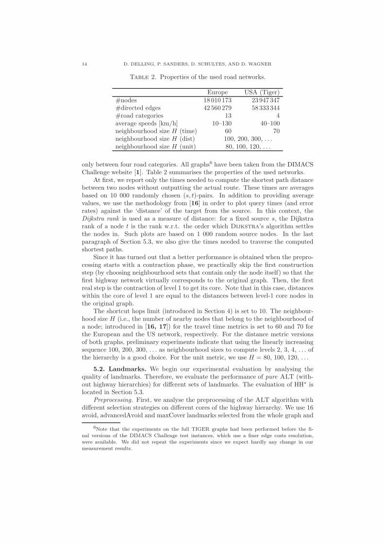
Table 2. Properties of the used road networks.
Europe USA (Tiger)#nodes 18 010 173 23 947 347#directed edges 42 560 279 58 333 344#road categories 13 4average speeds [km/h] 10–130 40–100neighbourhood size H (time) 60 70neighbourhood size H (dist) 100, 200, 300, . . .neighbourhood size H (unit) 80, 100, 120, . . .
only between four road categories. All graphs6 have been taken from the DIMACSChallenge website [1]. Table 2 summarises the properties of the used networks.
At first, we report only the times needed to compute the shortest path distancebetween two nodes without outputting the actual route. These times are averagesbased on 10 000 randomly chosen (s, t)-pairs. In addition to providing averagevalues, we use the methodology from [16] in order to plot query times (and errorrates) against the ‘distance’ of the target from the source. In this context, theDijkstra rank is used as a measure of distance: for a fixed source s, the Dijkstrarank of a node t is the rank w.r.t. the order which Dijkstra’s algorithm settlesthe nodes in. Such plots are based on 1 000 random source nodes. In the lastparagraph of Section 5.3, we also give the times needed to traverse the computedshortest paths.
Since it has turned out that a better performance is obtained when the prepro-cessing starts with a contraction phase, we practically skip the first constructionstep (by choosing neighbourhood sets that contain only the node itself) so that thefirst highway network virtually corresponds to the original graph. Then, the firstreal step is the contraction of level 1 to get its core. Note that in this case, distanceswithin the core of level 1 are equal to the distances between level-1 core nodes inthe original graph.
The shortcut hops limit (introduced in Section 4) is set to 10. The neighbour-hood size H (i.e., the number of nearby nodes that belong to the neighbourhood ofa node; introduced in [16, 17]) for the travel time metrics is set to 60 and 70 forthe European and the US network, respectively. For the distance metric versionsof both graphs, preliminary experiments indicate that using the linearly increasingsequence 100, 200, 300, . . . as neighbourhood sizes to compute levels 2, 3, 4, . . . ofthe hierarchy is a good choice. For the unit metric, we use H = 80, 100, 120, . . .
5.2. Landmarks. We begin our experimental evaluation by analysing thequality of landmarks. Therefore, we evaluate the performance of pure ALT (with-out highway hierarchies) for different sets of landmarks. The evaluation of HH∗ islocated in Section 5.3.
Preprocessing. First, we analyse the preprocessing of the ALT algorithm withdifferent selection strategies on different cores of the highway hierarchy. We use 16avoid, advancedAvoid and maxCover landmarks selected from the whole graph and
6Note that the experiments on the full TIGER graphs had been performed before the fi-nal versions of the DIMACS Challenge test instances, which use a finer edge costs resolution,were available. We did not repeat the experiments since we expect hardly any change in ourmeasurement results.
HIGHWAY HIERARCHIES STAR 15
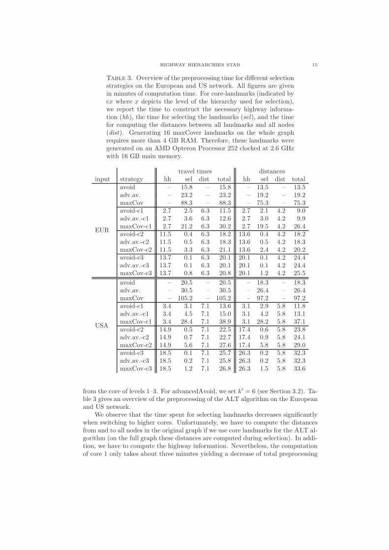
Table 3. Overview of the preprocessing time for different selectionstrategies on the European and US network. All figures are givenin minutes of computation time. For core-landmarks (indicated bycx where x depicts the level of the hierarchy used for selection),we report the time to construct the necessary highway informa-tion (hh), the time for selecting the landmarks (sel), and the timefor computing the distances between all landmarks and all nodes(dist). Generating 16 maxCover landmarks on the whole graphrequires more than 4 GB RAM. Therefore, these landmarks weregenerated on an AMD Opteron Processor 252 clocked at 2.6 GHzwith 16 GB main memory.
travel times distancesinput strategy hh sel dist total hh sel dist total
EUR
avoid – 15.8 – 15.8 – 13.5 – 13.5adv.av. – 23.2 – 23.2 – 19.2 – 19.2maxCov – 88.3 – 88.3 – 75.3 – 75.3avoid-c1 2.7 2.5 6.3 11.5 2.7 2.1 4.2 9.0adv.av.-c1 2.7 3.6 6.3 12.6 2.7 3.0 4.2 9.9maxCov-c1 2.7 21.2 6.3 30.2 2.7 19.5 4.2 26.4avoid-c2 11.5 0.4 6.3 18.2 13.6 0.4 4.2 18.2adv.av.-c2 11.5 0.5 6.3 18.3 13.6 0.5 4.2 18.3maxCov-c2 11.5 3.3 6.3 21.1 13.6 2.4 4.2 20.2avoid-c3 13.7 0.1 6.3 20.1 20.1 0.1 4.2 24.4adv.av.-c3 13.7 0.1 6.3 20.1 20.1 0.1 4.2 24.4maxCov-c3 13.7 0.8 6.3 20.8 20.1 1.2 4.2 25.5
USA
avoid – 20.5 – 20.5 – 18.3 – 18.3adv.av. – 30.5 – 30.5 – 26.4 – 26.4maxCov – 105.2 – 105.2 – 97.2 – 97.2avoid-c1 3.4 3.1 7.1 13.6 3.1 2.9 5.8 11.8adv.av.-c1 3.4 4.5 7.1 15.0 3.1 4.2 5.8 13.1maxCov-c1 3.4 28.4 7.1 38.9 3.1 28.2 5.8 37.1avoid-c2 14.9 0.5 7.1 22.5 17.4 0.6 5.8 23.8adv.av.-c2 14.9 0.7 7.1 22.7 17.4 0.9 5.8 24.1maxCov-c2 14.9 5.6 7.1 27.6 17.4 5.8 5.8 29.0avoid-c3 18.5 0.1 7.1 25.7 26.3 0.2 5.8 32.3adv.av.-c3 18.5 0.2 7.1 25.8 26.3 0.2 5.8 32.3maxCov-c3 18.5 1.2 7.1 26.8 26.3 1.5 5.8 33.6
from the core of levels 1–3. For advancedAvoid, we set k′ = 6 (see Section 3.2). Ta-ble 3 gives an overview of the preprocessing of the ALT algorithm on the Europeanand US network.
We observe that the time spent for selecting landmarks decreases significantlywhen switching to higher cores. Unfortunately, we have to compute the distancesfrom and to all nodes in the original graph if we use core landmarks for the ALT al-gorithm (on the full graph these distances are computed during selection). In addi-tion, we have to compute the highway information. Nevertheless, the computationof core 1 only takes about three minutes yielding a decrease of total preprocessing

16 D. DELLING, P. SANDERS, D. SCHULTES, AND D. WAGNER
with regard to all selection techniques. With regard to preprocessing time, usingavoid and advancedAvoid on the cores of level 2 or 3 does not seem reasonablewhile maxCover benefits from switching to higher cores.
Another advantage when switching to higher cores is memory consumption.While about 2.3 GB of RAM are needed for the distances from and to all nodeswhen selecting 16 avoid landmarks on the full graph, 384 MB are sufficient whenusing the core of level 1. Using the core-2 (core-3) even further reduces the memoryconsumption to 64 (17) MB. Note, that we use 32 bit integers for keeping thedistances in the main memory.
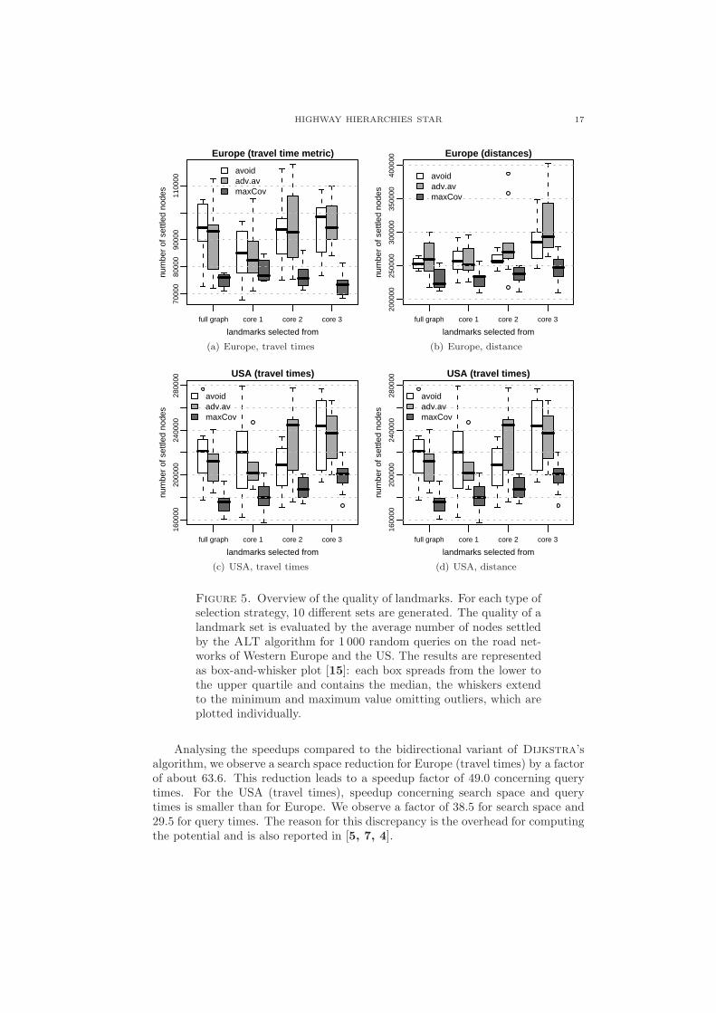
Quality of Landmarks. Figure 5 gives an overview of the quality of landmarks.Therefor, we generate 10 different sets of 16 landmarks for each selection strategy,generated on the full graph, and on the cores up to a level of 3. In order to evaluatethe quality of the generated landmarks, we logged the average search space for 1 000random s-t ALT-queries on the road network of Western Europe and the US. Theresults are presented as box-and-whisker plot [15].
We see that for distances the quality of landmarks is almost independent of thechosen level of the hierarchy. Only when switching from level 2 to 3 we observe amild increase of the search space when using advancedAvoid landmarks. However,for travel times on the European network an interesting phenomenon is that avoidgets better when switching from the whole graph to core 1 but gets worse andworse with higher levels on which landmarks are selected. On the US network, thesearch space reduces when switching to core 2 in combination with avoid landmarks.MaxCover is nearly independent of the chosen level on the European network whileon the US network a slight loss of quality can be observed with higher levels.
There seem to be two counteracting effects here: On higher levels of the hier-archy, we lose information. For example, peripheral nodes that are candidates forgood landmarks are dropped. On the other hand, concentrating on higher leveledges in landmark selection heuristics could be beneficial since these are edgesneeded by many shortest paths.
In general, maxCover outperforms avoid and advancedAvoid regarding the av-erage quality of the obtained landmarks. Nevertheless, in most cases the minimumaverage search space is nearly the same for all selection strategies within a core,while some sets of avoid and advancedAvoid landmarks lead to search spaces 25%higher than the worst maxCover landmarks. So, the maxCover routine seems to bemore robust than avoid or advancedAvoid. Comparing avoid and advancedAvoidwe observe just a mild improvement in quality. Thus, the additional computationtime of advancedAvoid is not worth the effort.
Combining the results from Table 3 and Figure 5, another strategy seemspromising: maxCover landmarks from the core of level 2 or 3 outperform avoidlandmarks from the full graph and their computation, including the highway in-formation, needs only additional 5 minutes compared to avoid landmarks from thefull graph. For this reason, we use such landmarks for our further experiments.
Efficiency and Approximation. Table 4 indicates the efficiency of our imple-mentation by reporting query times in comparison to the bidirectional variant ofDijkstra’s algorithm. For comparison with approximate HH queries we also pro-vide the results for an approximate ALT algorithm: Stop the query if the sum ofthe minimum keys in the forward and the backward queue exceed µ/(1+ ε)+pf(s)with ε = 0.1. This stopping criterion keeps the error rate below 10%.
HIGHWAY HIERARCHIES STAR 17
full graph core 1 core 2 core 3
7000
080
000
9000
011
0000
avoidadv.avmaxCov
Europe (travel time metric)
landmarks selected from
num
ber
of s
ettle
d no
des
(a) Europe, travel times
full graph core 1 core 2 core 3
2000
0025
0000
3000
0035
0000
4000
00
avoidadv.avmaxCov
Europe (distances)
landmarks selected from
num
ber
of s
ettle
d no
des
(b) Europe, distance
full graph core 1 core 2 core 3
1600
0020
0000
2400
0028
0000
avoidadv.avmaxCov
USA (travel times)
landmarks selected from
num
ber
of s
ettle
d no
des
(c) USA, travel times
full graph core 1 core 2 core 3
1600
0020
0000
2400
0028
0000
avoidadv.avmaxCov
USA (travel times)
landmarks selected from
num
ber
of s
ettle
d no
des
(d) USA, distance
Figure 5. Overview of the quality of landmarks. For each type ofselection strategy, 10 different sets are generated. The quality of alandmark set is evaluated by the average number of nodes settledby the ALT algorithm for 1 000 random queries on the road net-works of Western Europe and the US. The results are representedas box-and-whisker plot [15]: each box spreads from the lower tothe upper quartile and contains the median, the whiskers extendto the minimum and maximum value omitting outliers, which areplotted individually.
Analysing the speedups compared to the bidirectional variant of Dijkstra’salgorithm, we observe a search space reduction for Europe (travel times) by a factorof about 63.6. This reduction leads to a speedup factor of 49.0 concerning querytimes. For the USA (travel times), speedup concerning search space and querytimes is smaller than for Europe. We observe a factor of 38.5 for search space and29.5 for query times. The reason for this discrepancy is the overhead for computingthe potential and is also reported in [5, 7, 4].

18 D. DELLING, P. SANDERS, D. SCHULTES, AND D. WAGNER
Table 4. Comparison of the bidirectional variant of Dijkstra’salgorithm, the ALT algorithm, and the approximate ALT algo-rithm concerning search space, query times and error rate. Thelandmarks are 16 maxCover core-3 landmarks. The figures arebased on 1 000 random queries.
input metric bi.Dij. ALT approx.ALT
EUR
#settled nodes 4.68 · 106 73 563 61 939time query time [ms] 2 707 55.2 45.8
inaccurate queries – – 12.1%#settled nodes 5.27 · 106 241 476 219 124
dist query time [ms] 2 013 169.2 150.9inaccurate queries – – 33.7%
USA
#settled nodes 7.42 · 106 192 938 182 426time query time [ms] 3 808 129.2 116.9
inaccurate queries – – 8.9%#settled nodes 8.11 · 106 281 335 263 375
dist query time [ms] 3 437 177.1 163.5inaccurate queries – – 24.8%
For the distance metric on the European network we observe a reduction insearch space of factor 21.8, leading to a speedup factor of 11.8. The correspondingfigures for the US are 28.8 and 19.4. Thus, the situation is opposite to travel times.Here, speedups are better on the US network than on the European network. Thehigher speedups for travel times are due to the fact that for distances the advantageof taking fast highways instead of slow streets is smaller than for travel times. Sincethe difference between the slowest and fastest road category (see Table 2) is biggerfor Europe, the ALT algorithm performs better on this network than on the USnetwork when using travel times.
Comparing our results with the ones from [4] we have about 10% higher searchspaces on the US network (travel times). This derives from the fact that on theUS network with travel times the quality of maxCover landmarks slightly decreaseswhen switching to higher cores (see Figure 5). Nevertheless, our average querytimes in this instance are 2.49 (129 ms to 322 ms) times faster, although we areusing a slower computer. A reason for this is a different overhead factor, i.e., thetime spent per settled node. While our implementation has an overhead of factor1.3, the figures from [4] suggest an overhead of 2.
For the travel time metric, approximate queries perform only 20% better onEurope and 10% better on the US than exact ones. The percentage of inaccuratequeries is 12% and 8%, respectively. For the distance metric, the speedup forapproximate queries is even less and the percentage of inaccurate queries is muchhigher, namely 33.7% and 24.8% for the European and US network, respectively.These high numbers of wrong queries are due to the fact that for the distance metricthere are more possibilities of short paths with similar lengths since the differencebetween taking fast highways and driving on slow streets fades. So, approximationfor ALT adds only a small speedup not justifying the loss of correctness. For adetailed analysis of the approximation error see Table 10 and Figures 12–15 inAppendix A.

HIGHWAY HIERARCHIES STAR 19
211 212 213 214 215 216 217 218 219 220 221 222 223 224
0.1
110
100
1000
0.1
110
100
1000
EuropeUSA
Local Queries ALT (travel time metric)
Dijkstra Rank
Que
ry T
ime
[ms]
Figure 6. Comparison of the query times using the Dijkstra rankmethodology on the road networks of Europe and the US. Thelandmarks are chosen from the level-3 core using maxCover. Theresults are represented as box-and-whisker plot [15]: each boxspreads from the lower to the upper quartile and contains the me-dian, the whiskers extend to the minimum and maximum valueomitting outliers, which are plotted individually.
Local Queries. Figure 6 gives an overview of the query times in relation tothe Dijkstra rank. The results for the distance metric are located in Appendix A(Figure 9).
The fluctuations in query time both between different Dijkstra ranks and withfixed Dijkstra rank are so big that we had to use a logarithmic scale. Even typicalquery times vary by an order of magnitude for large Dijkstra ranks. The slowestqueries for most Dijkstra ranks are two orders of magnitude slower than the medianquery times.
An interesting observation is also that for small ranks ALT is faster on thenetwork of the US whereas for ranks higher than 221, queries are faster on theEuropean network. A plausible explanation seems to be the different geometry ofthe two continents. Queries within the (pen)insulae of Iberia, Britain, Italy, orScandinavia lack landmarks in many directions. For example, a user in Scotlandmight have the queer experience, that queries in north-south direction are consis-tently faster than queries in east-west direction (see Figure 3). In contrast, longdistance routes often have to go through bottlenecks which simplify search, as thosebottlenecks are part of many long distance routes. In the US, such effects are rare.
5.3. Highway Hierarchies and A∗ Search.
Default Settings. Unless otherwise stated, we use the following default settings.After the level-5 core has been determined, the construction of the hierarchy isstopped. A complete distance table is computed on the level-5 core. For the distancemetric, we stop at the level-6 core instead. We use 16 maxCover landmarks thathave been computed in the level-3 core. Landmark distances are stored only in the
20 D. DELLING, P. SANDERS, D. SCHULTES, AND D. WAGNER
level-1 core. The approximate query algorithm uses a maximum error rate of 10%,i.e., ε = 0.1.
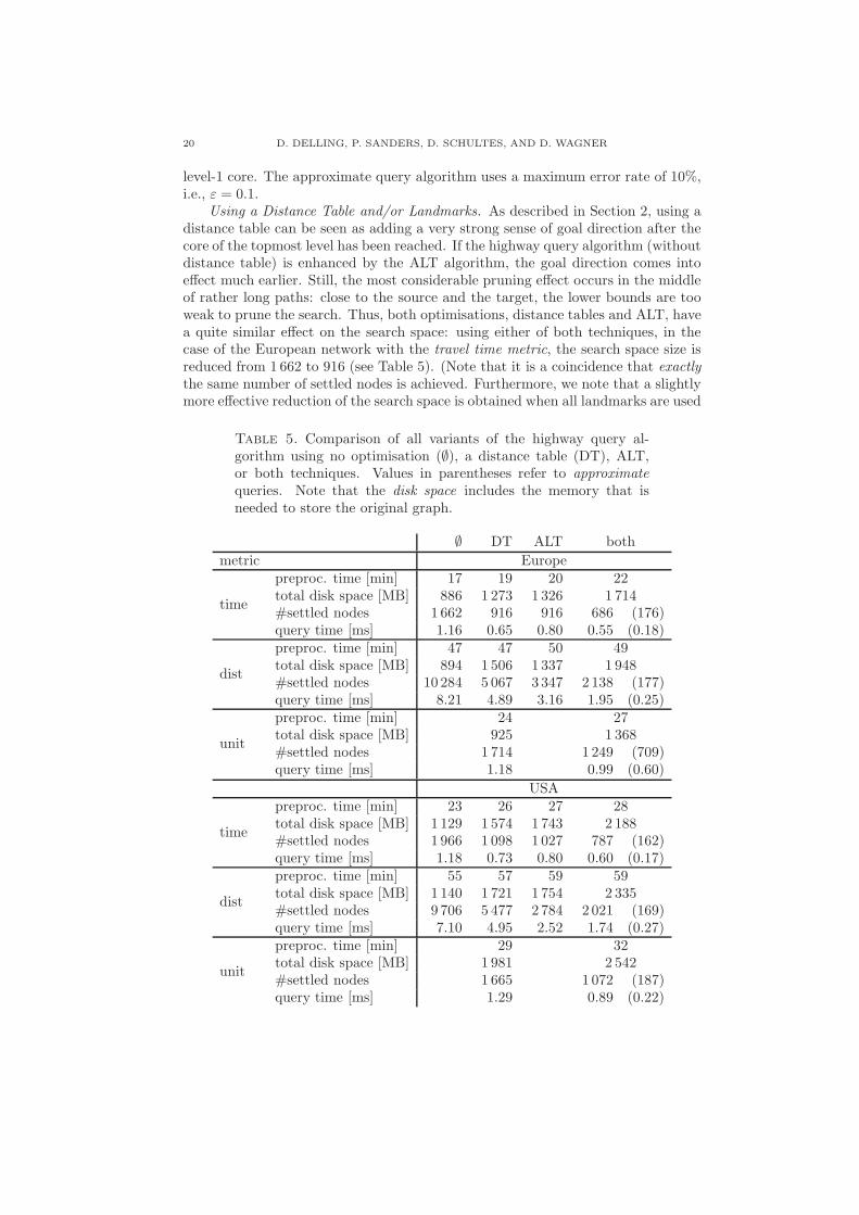
Using a Distance Table and/or Landmarks. As described in Section 2, using adistance table can be seen as adding a very strong sense of goal direction after thecore of the topmost level has been reached. If the highway query algorithm (withoutdistance table) is enhanced by the ALT algorithm, the goal direction comes intoeffect much earlier. Still, the most considerable pruning effect occurs in the middleof rather long paths: close to the source and the target, the lower bounds are tooweak to prune the search. Thus, both optimisations, distance tables and ALT, havea quite similar effect on the search space: using either of both techniques, in thecase of the European network with the travel time metric, the search space size isreduced from 1 662 to 916 (see Table 5). (Note that it is a coincidence that exactlythe same number of settled nodes is achieved. Furthermore, we note that a slightlymore effective reduction of the search space is obtained when all landmarks are used
Table 5. Comparison of all variants of the highway query al-gorithm using no optimisation (∅), a distance table (DT), ALT,or both techniques. Values in parentheses refer to approximatequeries. Note that the disk space includes the memory that isneeded to store the original graph.
∅ DT ALT both
metric Europe
time
preproc. time [min] 17 19 20 22total disk space [MB] 886 1 273 1 326 1 714#settled nodes 1 662 916 916 686 (176)query time [ms] 1.16 0.65 0.80 0.55 (0.18)
dist
preproc. time [min] 47 47 50 49total disk space [MB] 894 1 506 1 337 1 948#settled nodes 10 284 5 067 3 347 2 138 (177)query time [ms] 8.21 4.89 3.16 1.95 (0.25)
unit
preproc. time [min] 24 27total disk space [MB] 925 1 368#settled nodes 1 714 1 249 (709)query time [ms] 1.18 0.99 (0.60)
USA
time
preproc. time [min] 23 26 27 28total disk space [MB] 1 129 1 574 1 743 2 188#settled nodes 1 966 1 098 1 027 787 (162)query time [ms] 1.18 0.73 0.80 0.60 (0.17)
dist
preproc. time [min] 55 57 59 59total disk space [MB] 1 140 1 721 1 754 2 335#settled nodes 9 706 5 477 2 784 2 021 (169)query time [ms] 7.10 4.95 2.52 1.74 (0.27)
unit
preproc. time [min] 29 32total disk space [MB] 1 981 2 542#settled nodes 1 665 1 072 (187)query time [ms] 1.29 0.89 (0.22)
HIGHWAY HIERARCHIES STAR 21
to compute lower bounds instead of selecting only one landmark for each direction,namely to 903 instead of 916.) When we consider other aspects like preprocessingtime, memory usage, and query time, we can conclude that the distance table issomewhat superior to the landmarks optimisation. Since both techniques have asimilar point of application, a combination of the highway query algorithm withboth optimisations gives only a comparatively small improvement compared tousing only one optimisation. In contrast to the exact algorithm, the approximatevariant reduces the search space size and the query time considerably—e.g., to 19%and 27% in case of Europe (relative to using only the distance table optimisation)—, while guaranteeing a maximum error of 10% and achieving a total error of 0.056%in our random sample of 1 000 000 (s, t)-pairs (refer to Table 7). Some results forUS subgraphs can be found in Table 9 in Appendix A.
Using a distance metric, ALT gets more effective and beats the distance tableoptimisation since much better lower bounds are produced: the negative effect de-scribed in Figure 4 is weakened. Furthermore, in this case, a combination with bothoptimisations is worthwhile: the query time is reduced to 40% in case of Europe(relative to using only the distance table optimisation). While the highway queryalgorithm enhanced with a distance table has 7.5 times slower query times whenapplied to the European graph with the distance metric instead of using the traveltime metric, the combination with both optimisations reduces this performancedifference to a factor of 3.5—or even 1.4 when the approximate variant is used.
The performance for the unit metric ranks somewhere in between. Althoughcomputing shortest paths in road networks based on the unit metric seems kind ofartificial, we observe a hierarchy in this scenario as well, which explains the sur-prisingly good preprocessing and query times: when we drive on urban streets, weencounter much more junctions than driving on a national road or even a motor-way; thus, the number of road segments on a path is somewhat correlated to theroad type.
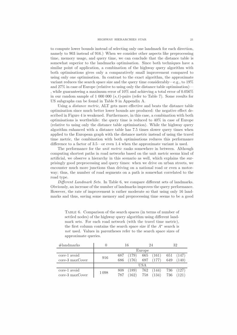
Different Landmark Sets. In Table 6, we compare different sets of landmarks.Obviously, an increase of the number of landmarks improves the query performance.However, the rate of improvement is rather moderate so that using only 16 land-marks and thus, saving some memory and preprocessing time seems to be a good
Table 6. Comparison of the search spaces (in terms of number ofsettled nodes) of the highway query algorithm using different land-mark sets. For each road network (with the travel time metric),the first column contains the search space size if the A∗ search isnot used. Values in parentheses refer to the search space sizes ofapproximate queries.
#landmarks 0 16 24 32
Europecore-1 avoid
916687 (179) 665 (161) 651 (147)
core-3 maxCover 686 (176) 697 (177) 649 (140)
USAcore-1 avoid
1 098808 (189) 762 (144) 736 (127)
core-3 maxCover 787 (162) 758 (134) 736 (121)
22 D. DELLING, P. SANDERS, D. SCHULTES, AND D. WAGNER
option. The quality of the selected landmarks is very similar for the two land-mark selection methods that we have considered. Since the preprocessing timesare similar as well, we prefer using the maxCover landmarks since they are slightlybetter.
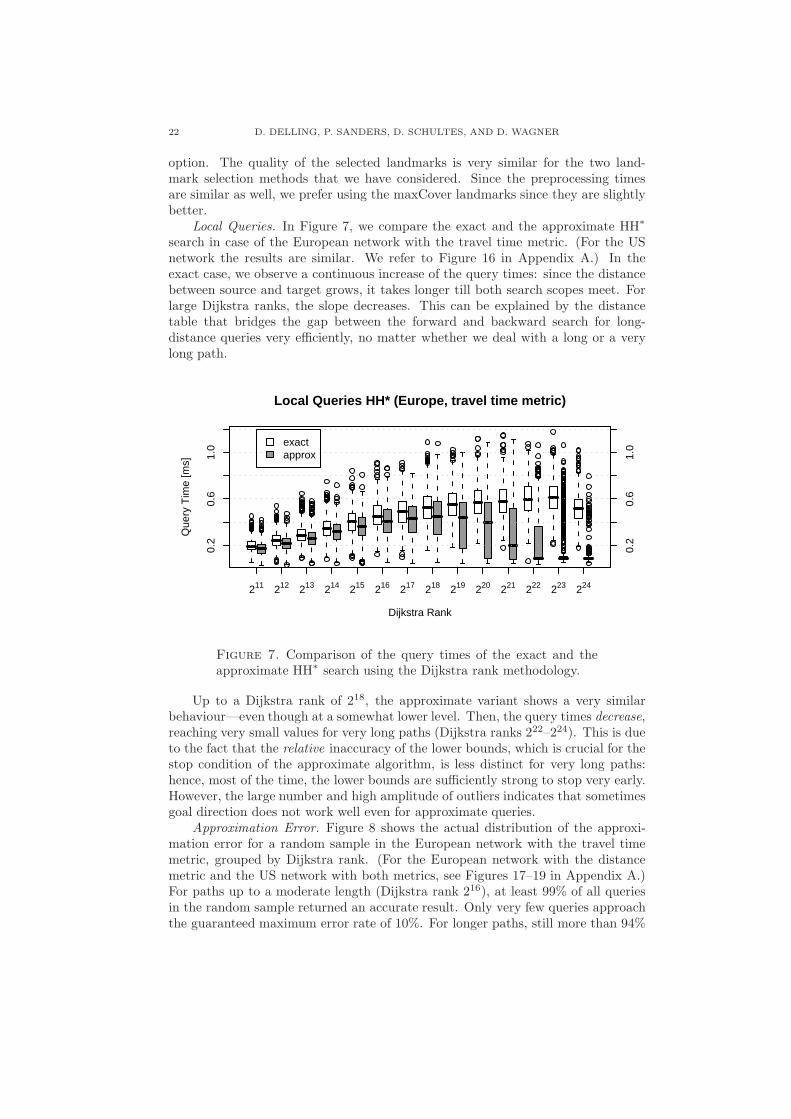
Local Queries. In Figure 7, we compare the exact and the approximate HH∗
search in case of the European network with the travel time metric. (For the USnetwork the results are similar. We refer to Figure 16 in Appendix A.) In theexact case, we observe a continuous increase of the query times: since the distancebetween source and target grows, it takes longer till both search scopes meet. Forlarge Dijkstra ranks, the slope decreases. This can be explained by the distancetable that bridges the gap between the forward and backward search for long-distance queries very efficiently, no matter whether we deal with a long or a verylong path.
Local Queries HH* (Europe, travel time metric)
Dijkstra Rank
Que
ry T
ime
[ms]
211 212 213 214 215 216 217 218 219 220 221 222 223 224
0.2
0.6
1.0
0.2
0.6
1.0exact
approx
Figure 7. Comparison of the query times of the exact and theapproximate HH∗ search using the Dijkstra rank methodology.
Up to a Dijkstra rank of 218, the approximate variant shows a very similarbehaviour—even though at a somewhat lower level. Then, the query times decrease,reaching very small values for very long paths (Dijkstra ranks 222–224). This is dueto the fact that the relative inaccuracy of the lower bounds, which is crucial for thestop condition of the approximate algorithm, is less distinct for very long paths:hence, most of the time, the lower bounds are sufficiently strong to stop very early.However, the large number and high amplitude of outliers indicates that sometimesgoal direction does not work well even for approximate queries.
Approximation Error. Figure 8 shows the actual distribution of the approxi-mation error for a random sample in the European network with the travel timemetric, grouped by Dijkstra rank. (For the European network with the distancemetric and the US network with both metrics, see Figures 17–19 in Appendix A.)For paths up to a moderate length (Dijkstra rank 216), at least 99% of all queriesin the random sample returned an accurate result. Only very few queries approachthe guaranteed maximum error rate of 10%. For longer paths, still more than 94%

HIGHWAY HIERARCHIES STAR 23
of the queries give the correct result, and almost 99% of the queries find paths thatare at most 2% longer than the shortest path. The fact that we get more errorsfor longer paths corresponds to the running times depicted in Figure 7: in the caseof large Dijkstra ranks, we usually stop the search quite early, which increases thelikelihood of an inaccuracy.
Approximation Error HH* (Europe, travel time metric)
Dijkstra Rank
Per
cent
age
211 212 213 214 215 216 217 218 219 220 221 222 223 224
9495
9697
9899
9495
9697
9899
up to 10% longerup to 8% longerup to 6% longerup to 4% longerup to 2% longeraccurate
Figure 8. Actual distribution of the approximation error for arandom sample, grouped by Dijkstra rank. Note that, in order toincrease readability, the y-axis starts at 94%, i.e., at least 94% ofall queries returned an accurate result.
While the approximate variant of the ALT algorithm gives only a small speedup(compare Figure 6 with Figure 10 in Appendix A) and produces a considerableamount of inaccurate results (in particular for short paths, see Figures 12 and 14),the approximate HH∗ algorithm is much faster than the exact version (in particularfor long paths) and produces a comparatively small amount of inaccurate results.This difference is mainly due to the distance table, which allows a fast determinationof upper bounds—and thus, in many cases early aborts—and provides accuratelong-distance subpaths, i.e., the only thing that can go wrong is that the searchprocesses in the local area around source and target do not find the right coreentrance points.
In Table 7, we compared the effect of different maximum error rates ε. Weobtained the expected result that a larger maximum error rate reduces the searchspace size considerably. Furthermore, we had a look at the actual error that occursin our random sample: we divided the sum of all path lengths that were obtained bythe approximate algorithm by the sum of the shortest path lengths. We find that theresulting total error is very small, e.g., only 0.056% in case of the European networkwith the travel time metric when we allow a maximum error rate of 10%. Similarto the results in Section 5.2, we observe that the total error and the percentage ofinaccurate queries (see Figures 17 and 19) are much higher when using the distancemetric instead of the travel time metric.
24 D. DELLING, P. SANDERS, D. SCHULTES, AND D. WAGNER
Table 7. Comparison of different maximum error rates ε. By thetotal error, we give the sum of the path lengths obtained by theapproximate algorithm divided by the sum of the shortest pathlengths. Note that these values are given in percent. This table isbased on 1 000 000 random (s, t)-pairs (instead of the usual 10 000pairs).
ε [%] 0 1 2 5 10 20
metric Europe
time#settled nodes 685 612 523 319 177 103total error [%] 0 0.0002 0.0015 0.018 0.056 0.112
dist#settled nodes 2131 1302 843 333 184 143total error [%] 0 0.0112 0.0383 0.172 0.329 0.526
USA
time#settled nodes 784 632 516 307 162 86total error [%] 0 0.0013 0.0073 0.034 0.082 0.144
dist#settled nodes 2021 1101 672 277 169 134total error [%] 0 0.0108 0.0441 0.132 0.193 0.240
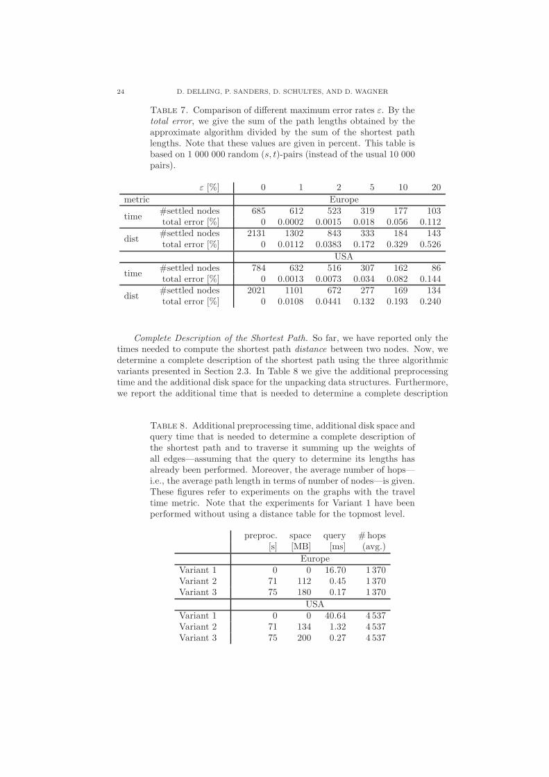
Complete Description of the Shortest Path. So far, we have reported only thetimes needed to compute the shortest path distance between two nodes. Now, wedetermine a complete description of the shortest path using the three algorithmicvariants presented in Section 2.3. In Table 8 we give the additional preprocessingtime and the additional disk space for the unpacking data structures. Furthermore,we report the additional time that is needed to determine a complete description
Table 8. Additional preprocessing time, additional disk space andquery time that is needed to determine a complete description ofthe shortest path and to traverse it summing up the weights ofall edges—assuming that the query to determine its lengths hasalready been performed. Moreover, the average number of hops—i.e., the average path length in terms of number of nodes—is given.These figures refer to experiments on the graphs with the traveltime metric. Note that the experiments for Variant 1 have beenperformed without using a distance table for the topmost level.
preproc. space query #hops[s] [MB] [ms] (avg.)
EuropeVariant 1 0 0 16.70 1 370Variant 2 71 112 0.45 1 370Variant 3 75 180 0.17 1 370
USAVariant 1 0 0 40.64 4 537Variant 2 71 134 1.32 4 537Variant 3 75 200 0.27 4 537
HIGHWAY HIERARCHIES STAR 25
of the shortest path and to traverse7 it summing up the weights of all edges as asanity check—assuming that the distance query has already been performed. Thatmeans that the total average time to determine a shortest path is the time given inTable 8 plus the query time given in previous tables. We can conclude that evenVariant 3 uses comparatively little preprocessing time and space. With Variant 3,the time for outputting the path remains considerably smaller than the query timeitself and a factor 3–5 smaller than using Variant 2. The USA graph profits morethan the European graph since it has paths with considerably larger hop counts,perhaps due to a larger number of degree-two nodes in the input. Note that dueto cache effects, the time for outputting the path using preprocessed shortcuts islikely to be considerably smaller than the time for traversing the shortest path inthe original graph.
6. Discussion
We have learned a few things about landmark A∗ (ALT) that are interestingindependently of highway hierarchies. We have explained why the lower boundsprovided by ALT are often quite weak and why there are very high fluctuations inquery performance. There are also considerable differences between Western Europeand the US. In Europe, we have larger execution times for local queries than inthe US whereas for long range (average case) queries, times are smaller. Executinglandmark selection on a graph where sparse subgraphs have been contracted isprofitable in terms of preprocessing time even if we do not want highway hierarchies.Similarly, storing distances to landmarks only on this contracted graph considerablyreduces the space overhead of ALT.
For highway hierarchies we have learned that they can also handle the case oftravel distances. Compared to the case of travel times, space consumption is roughlythe same whereas preprocessing time and query time increase by a factor of about2–3.5 (when the combination with A∗ search is applied). It is to be expected thatany other cost metric that represents some compromise of travel time, distance,fuel consumption and tolls will have performance somewhere within this range.Highway hierarchies can be augmented to output shortest paths in a time belowthe time needed for computing the distances.
There is a complex interplay between highway hierarchies and the optimisationsof distance tables and ALT. For exact queries using the travel time metric, distancetables are a better investment into preprocessing time and space than ALT. Oneincompatibility between highway hierarchies and ALT is that the search cannot bestopped when search frontiers meet. For approximate queries or for the distancemetric, all three techniques work together very well yielding a speedup aroundfour over highway hierarchies alone: Highway hierarchies save space and time forlandmark preprocessing; distance tables obviate search in higher levels and allowsimpler and faster ALT search with very effective goal direction. ALT providesgood pruning opportunities for the distance metric and an excellent sense of goaldirection for approximate queries yielding high quality routes most of the time whilenever computing very bad routes.
7Note that we do not traverse the path in the original graph, but we directly scan theassembled description of the path.

26 D. DELLING, P. SANDERS, D. SCHULTES, AND D. WAGNER
An interesting route of future research is to consider a combination of highwayhierarchies with geometric containers or edge flags [20, 13, 11]. Highway hierar-chies might harmonise better with these methods than with ALT because similarto highway hierarchies they are based on truncating search at certain edges. Thereis also hope that their high preprocessing costs might be reduced by exploiting thehighway hierarchy.
Very recently, transit node routing (TNR) and related approaches [14, 2] haveaccelerated shortest path queries by another two orders of magnitude. Roughly,TNR precomputes shortest path distances to access points in a transit node setT (e.g., the nodes at the highest level of the highway hierarchy). During a querybetween “sufficiently distant” nodes, a distance table for T can be used to bridgethe gap between the access points of source and target. However, TNR needsconsiderably more preprocessing time than the approach described in this paper.Furthermore, the currently best implementation of TNR uses highway hierarchiesfor preprocessing and local queries. It is likely that also landmarks might turn outto be useful in future versions of TNR. On the one hand, landmarks yield lowerbounds that can be used for locality filters needed in TNR. On the other hand, theprecomputed distances to access points could be used as landmark information forspeeding up local search.
Acknowledgements. We would like to thank Timo Bingmann for work onvisualisation tools. Two anonymous reviewers provided valuable suggestions.
References
1. 9th DIMACS Implementation Challenge, Shortest Paths, http://www.dis.uniroma1.it/∼challenge9/, 2006.
2. H. Bast, S. Funke, D. Matijevic, P. Sanders, and D. Schultes, In transit to constant timeshortest-path queries in road networks, Workshop on Algorithm Engineering and Experiments,2007.
3. E. W. Dijkstra, A note on two problems in connexion with graphs., Numerische Mathematik1 (1959), 269–271.
4. A. Goldberg, H. Kaplan, and R. Werneck, Reach for A∗: Efficient point-to-point shortest pathalgorithms, Workshop on Algorithm Engineering & Experiments (Miami), 2006, pp. 129–143.
5. A. V. Goldberg and C. Harrelson, Computing the shortest path: A∗ meets graph theory, 16thACM-SIAM Symposium on Discrete Algorithms, 2005, pp. 156–165.
6. A. V. Goldberg, H. Kaplan, and R. F. Werneck, Better landmarks within reach, 9th DIMACSImplementation Challenge [1], 2006.
7. A. V. Goldberg and R. F. Werneck, An efficient external memory shortest path algorithm,Workshop on Algorithm Engineering and Experimentation, 2005, pp. 26–40.
8. R. Gutman, Reach-based routing: A new approach to shortest path algorithms optimized forroad networks, 6th Workshop on Algorithm Engineering and Experiments, 2004, pp. 100–111.
9. P. E. Hart, N. J. Nilsson, and B. Raphael, A formal basis for the heuristic determination ofminimum cost paths, IEEE Transactions on System Science and Cybernetics 4 (1968), no. 2,100–107.
10. T. Ikeda, M.Y. Hsu, H. Imai, S. Nishimura, H. Shimoura, T. Hashimoto, K. Tenmoku, andK. Mitoh, A fast algorithm for finding better routes by AI search techniques, Vehicle Naviga-tion and Information Systems Conference. IEEE, 1994.
11. U. Lauther, An extremely fast, exact algorithm for finding shortest paths in static networkswith geographical background, Geoinformation und Mobilitat – von der Forschung zur praktis-
chen Anwendung, vol. 22, IfGI prints, Institut fur Geoinformatik, Munster, 2004, pp. 219–230.12. J. Maue, P. Sanders, and D. Matijevic, Goal directed shortest path queries using
Precomputed Cluster Distances, 5th Workshop on Experimental Algorithms (WEA), LNCS,no. 4007, Springer, 2006, pp. 316–328.

HIGHWAY HIERARCHIES STAR 27
13. R. H. Mohring, H. Schilling, B. Schutz, D. Wagner, and T. Willhalm, Partitioning graphsto speed up Dijkstra’s algorithm, 4th International Workshop on Efficient and ExperimentalAlgorithms, 2005, pp. 189–202.
14. K. Muller, Design and implementation of an efficient hierarchical speed-up technique forcomputation of exact shortest paths in graphs, Master’s thesis, Universtat Karlsruhe, 2006,supervised by D. Delling, M. Holzer, F. Schulz, and D. Wagner.
15. R Development Core Team, R: A Language and Environment for Statistical Computing,http://www.r-project.org, 2004.
16. P. Sanders and D. Schultes, Highway hierarchies hasten exact shortest path queries, 13thEuropean Symposium on Algorithms, LNCS, vol. 3669, Springer, 2005, pp. 568–579.
17. P. Sanders and D. Schultes, Engineering highway hierarchies, 14th European Symposium onAlgorithms, LNCS, vol. 4168, Springer, 2006, pp. 804–816.
18. R. Sedgewick and J. S. Vitter, Shortest paths in Euclidean space, Algorithmica 1 (1986),31–48.
19. U.S. Census Bureau, Washington, DC, UA Census 2000 TIGER/Line Files, http://www.
census.gov/geo/www/tiger/tigerua/ua tgr2k.html, 2002.20. D. Wagner and T. Willhalm, Geometric speed-up techniques for finding shortest paths in large
sparse graphs, 11th European Symposium on Algorithms, LNCS, vol. 2832, Springer, 2003,pp. 776–787.
21. T. Willhalm, Engineering shortest path and layout algorithms for large graphs, Ph.D. thesis,Universitat Karlsruhe (TH), Fakultat fur Informatik, 2005.
Appendix A. Further Experiments
Table 9. Performance of HH∗ (using a distance table and land-marks) for US subgraphs with travel time metric. For small graphs,we deviate from the default settings: the landmark selection takesplace in the core of the level given in column 2, the constructionof the highway hierarchy is stopped at the core of the level givenin column 3.
landm. sel. dist. table preproc. total disk #settled querygraph core level core level time [min] space [MB] nodes time [ms]NY 2 3 0:55 140 334 0.22BAY 2 3 0:24 40 329 0.20COL 2 3 0:29 49 327 0.19FLA 3 3 1:08 115 354 0.22NW 3 4 1:06 87 509 0.33NE 3 4 2:14 169 526 0.36
CAL 3 4 2:23 176 519 0.35LKS 3 4 4:25 398 543 0.39E 3 5 4:07 255 650 0.46W 3 5 7:22 453 695 0.50
CTR 3 5 23:12 1 132 762 0.73

28 D. DELLING, P. SANDERS, D. SCHULTES, AND D. WAGNER
211 212 213 214 215 216 217 218 219 220 221 222 223 224
0.1
110
100
1000
0.1
110
100
1000
EuropeUSA
Local Queries ALT (distance metric)
Dijkstra Rank
Que
ry T
ime
[ms]
Figure 9. Comparison of the query times on the road networkof Western Europe and the USA using the ALT algorithm. Thelandmarks are chosen from the core-3 using maxCover.
Table 10. Comparison of the exact and approximate ALT algo-rithm. The landmarks are taken from the full graph. The figuresare based on 1 000 random queries on 10 different sets of 16 land-marks.
#settled nodes inaccurate queriesinput metric landmarks exact approx. min – max
EUR
avoid 93 520 81 582 9.8% – 11.9%time adv.av. 86 340 74 706 9.3% – 12.6%
maxCover 75 220 63 112 10.7% – 11.7%avoid 253 552 225 618 31.5% – 38.4%
dist adv.av. 256 511 227 779 30.9% – 38.0%maxCover 230 110 203 564 31.3% – 34.9%
USA
avoid 220 333 206 165 7.4% – 10.1%time adv.av. 210 703 194 920 7.6% – 9.6%
maxCover 175 359 161 230 7.6% – 9.6%avoid 308 823 289 701 24.8% – 29.9%
dist adv.av. 302 521 282 410 24.3% – 29.3%maxCover 282 162 265 091 27.3% – 22.3%
HIGHWAY HIERARCHIES STAR 29
211 212 213 214 215 216 217 218 219 220 221 222 223 224
0.1
110
100
1000
0.1
110
100
1000
EuropeUSA
Local Queries approximate ALT (travel times metric)
Dijkstra Rank
Que
ry T
ime
[ms]
Figure 10. Comparison of the query times on the road networkof Western Europe and the USA using the approximate ALT al-gorithm. The landmarks are chosen from the core-3 using max-Cover.
211 212 213 214 215 216 217 218 219 220 221 222 223 224
0.1
110
100
1000
0.1
110
100
1000
EuropeUSA
Local Queries approximate ALT (distance metric)
Dijkstra Rank
Que
ry T
ime
[ms]
Figure 11. Comparison of the query times on the road networkof Western Europe and the USA using the approximate ALT al-gorithm. The landmarks are chosen from the core-3 using max-Cover.

30 D. DELLING, P. SANDERS, D. SCHULTES, AND D. WAGNER
Approximation Error ALT (Europe, travel time metric)
Dijkstra Rank
Per
cent
age
211 212 213 214 215 216 217 218 219 220 221 222 223 224
8590
9510
0
8590
9510
0
up to 10% longerup to 8% longerup to 6% longerup to 4% longerup to 2% longeraccurate
Figure 12. Actual distribution of the approximation error for arandom sample, grouped by Dijkstra rank. Note that, in order toincrease readability, the y-axis starts at 85%, i.e., at least 50% ofall queries returned an accurate result.
Approximation Error ALT (Europe, distance metric)
Dijkstra Rank
Per
cent
age
211 212 213 214 215 216 217 218 219 220 221 222 223 224
5060
7080
9010
0
5060
7080
9010
0
up to 10% longerup to 8% longerup to 6% longerup to 4% longerup to 2% longeraccurate
Figure 13. Actual distribution of the approximation error for arandom sample, grouped by Dijkstra rank. Note that, in order toincrease readability, the y-axis starts at 50%, i.e., at least 50% ofall queries returned an accurate result.
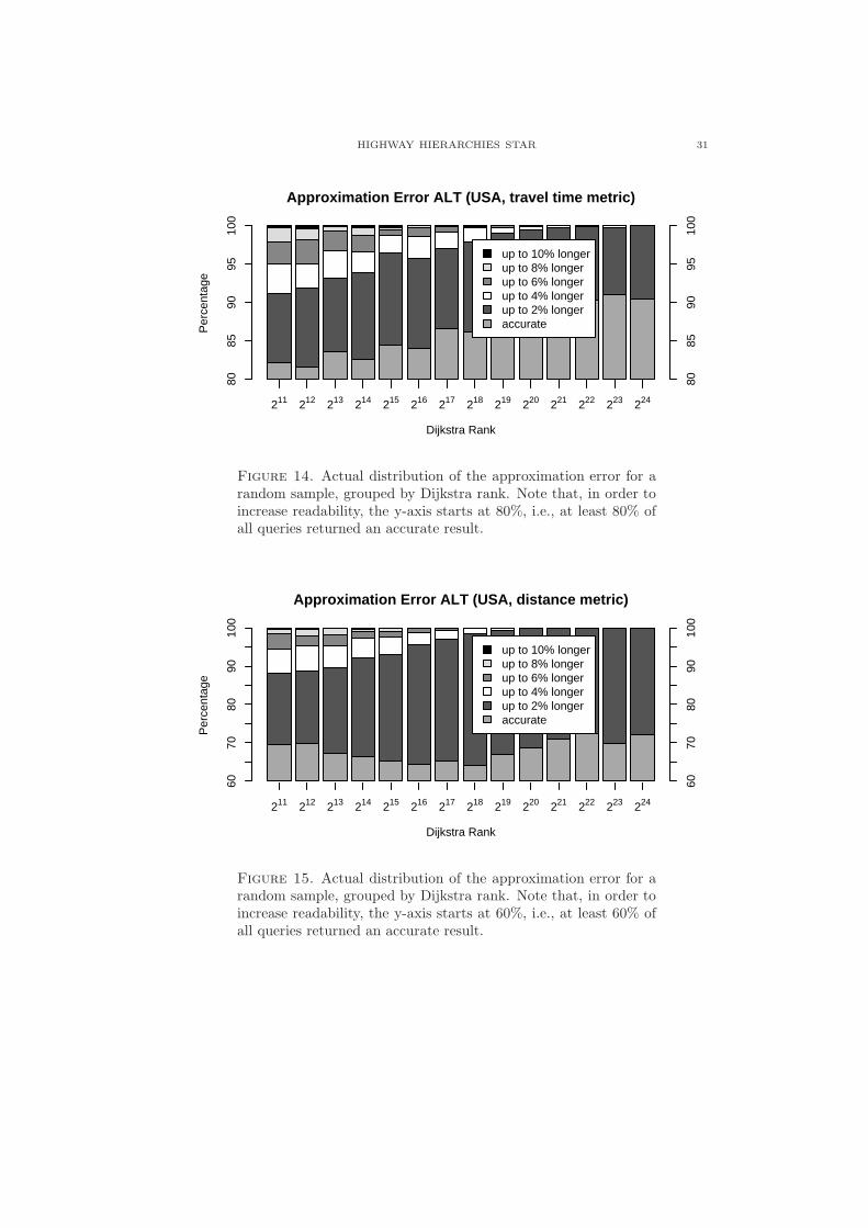
HIGHWAY HIERARCHIES STAR 31
Approximation Error ALT (USA, travel time metric)
Dijkstra Rank
Per
cent
age
211 212 213 214 215 216 217 218 219 220 221 222 223 224
8085
9095
100
8085
9095
100
up to 10% longerup to 8% longerup to 6% longerup to 4% longerup to 2% longeraccurate
Figure 14. Actual distribution of the approximation error for arandom sample, grouped by Dijkstra rank. Note that, in order toincrease readability, the y-axis starts at 80%, i.e., at least 80% ofall queries returned an accurate result.
Approximation Error ALT (USA, distance metric)
Dijkstra Rank
Per
cent
age
211 212 213 214 215 216 217 218 219 220 221 222 223 224
6070
8090
100
6070
8090
100
up to 10% longerup to 8% longerup to 6% longerup to 4% longerup to 2% longeraccurate
Figure 15. Actual distribution of the approximation error for arandom sample, grouped by Dijkstra rank. Note that, in order toincrease readability, the y-axis starts at 60%, i.e., at least 60% ofall queries returned an accurate result.

32 D. DELLING, P. SANDERS, D. SCHULTES, AND D. WAGNER
Local Queries HH* (USA, travel time metric)
Dijkstra Rank
Que
ry T
ime
[ms]
211 212 213 214 215 216 217 218 219 220 221 222 223 224
0.2
0.6
1.0
0.2
0.6
1.0exact
approx
Figure 16. Comparison of the query times of the exact and theapproximate HH∗ search.
Approximation Error HH* (Europe, distance metric)
Dijkstra Rank
Per
cent
age
211 212 213 214 215 216 217 218 219 220 221 222 223 224
7075
8085
9095
7075
8085
9095
up to 10% longerup to 8% longerup to 6% longerup to 4% longerup to 2% longeraccurate
Figure 17. Actual distribution of the approximation error for arandom sample, grouped by Dijkstra rank. Note that, in order toincrease readability, the y-axis starts at 70%, i.e., at least 70% ofall queries returned an accurate result.

HIGHWAY HIERARCHIES STAR 33
Approximation Error HH* (USA, travel time metric)
Dijkstra Rank
Per
cent
age
211 212 213 214 215 216 217 218 219 220 221 222 223 224
8890
9294
9698
8890
9294
9698
up to 10% longerup to 8% longerup to 6% longerup to 4% longerup to 2% longeraccurate
Figure 18. Actual distribution of the approximation error for arandom sample, grouped by Dijkstra rank. Note that, in order toincrease readability, the y-axis starts at 88%, i.e., at least 88% ofall queries returned an accurate result.
Approximation Error HH* (USA, distance metric)
Dijkstra Rank
Per
cent
age
211 212 213 214 215 216 217 218 219 220 221 222 223 224
7580
8590
9510
0
7580
8590
9510
0up to 10% longerup to 8% longerup to 6% longerup to 4% longerup to 2% longeraccurate
Figure 19. Actual distribution of the approximation error for arandom sample, grouped by Dijkstra rank. Note that, in order toincrease readability, the y-axis starts at 75%, i.e., at least 75% ofall queries returned an accurate result.
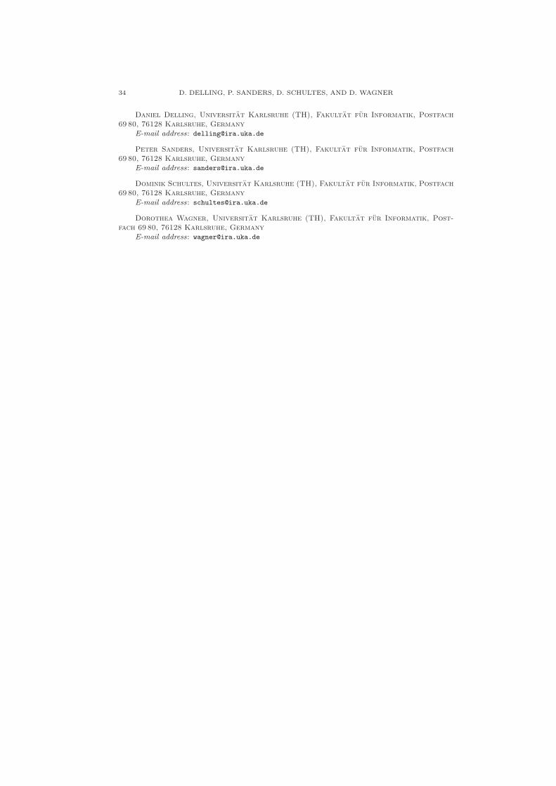
34 D. DELLING, P. SANDERS, D. SCHULTES, AND D. WAGNER
Daniel Delling, Universitat Karlsruhe (TH), Fakultat fur Informatik, Postfach69 80, 76128 Karlsruhe, Germany
E-mail address: [email protected]
Peter Sanders, Universitat Karlsruhe (TH), Fakultat fur Informatik, Postfach69 80, 76128 Karlsruhe, Germany
E-mail address: [email protected]
Dominik Schultes, Universitat Karlsruhe (TH), Fakultat fur Informatik, Postfach69 80, 76128 Karlsruhe, Germany
E-mail address: [email protected]
Dorothea Wagner, Universitat Karlsruhe (TH), Fakultat fur Informatik, Post-fach 69 80, 76128 Karlsruhe, Germany
E-mail address: [email protected]