
Highway Engineering - GeoCitiesengineering.pdfHIGHWAY ENGINEERING ... 2.1 Basic principles of...
292
HIGHWAY ENGINEERING
Transcript of Highway Engineering - GeoCitiesengineering.pdfHIGHWAY ENGINEERING ... 2.1 Basic principles of...

HIGHWAY ENGINEERING


HIGHWAYENGINEERINGMartin RogersDepartment of Civil and Structural EngineeringDublin Institute of TechnologyIreland
BlackwellScience

© 2003 by Blackwell Publishing LtdEditorial Offices:9600 Garsington Road, Oxford OX4 2DQ
Tel: +44 (0) 1865 776868108 Cowley Road, Oxford OX4 1JF, UK
Tel: +44 (0)1865 791100Blackwell Publishing USA, 350 MainStreet, Malden, MA 02148-5018, USA
Tel: +1 781 388 8250Iowa State Press, a Blackwell PublishingCompany, 2121 State Avenue, Ames, Iowa50014-8300, USA
Tel: +1 515 292 0140Blackwell Munksgaard, 1 Rosenørns Allé,P.O. Box 227, DK-1502 Copenhagen V,Denmark
Tel: +45 77 33 33 33Blackwell Publishing Asia Pty Ltd,550 Swanston Street, Carlton South,Victoria 3053, Australia
Tel: +61 (0)3 9347 0300Blackwell Verlag, Kurfürstendamm 57,10707 Berlin, Germany
Tel: +49 (0)30 32 79 060Blackwell Publishing, 10 rue CasimirDelavigne, 75006 Paris, France
Tel: +33 1 53 10 33 10
The right of the Author to be identified as the Authorof this Work has been asserted in accordance with theCopyright, Designs and Patents Act 1988.
All rights reserved. No part of this publication maybe reproduced, stored in a retrieval system, ortransmitted, in any form or by any means, electronic,mechanical, photocopying, recording or otherwise,except as permitted by the UK Copyright, Designsand Patents Act 1988, without the prior permission of the publisher.
First published 2003
A catalogue record for this title is available from theBritish Library
ISBN 0-632-05993-1
Library of CongressCataloging-in-Publication DataRogers, Martin.
Highway engineering / Martin Rogers. – 1st ed.p. cm.
ISBN 0-632-05993-1 (Paperback : alk. paper)1. Highway engineering. I. Title.TE145.R65 2003625.7 – dc21
2003005910
Set in 10 on 13 pt Timesby SNP Best-set Typesetter Ltd., Hong KongPrinted and bound in Great Britain byTJ International Ltd, Padstow, Cornwall
For further information onBlackwell Publishing, visit our website:www.blackwellpublishing.com

To Margaret, for all her love, support and encouragement

Contents
Preface, xiiiAcknowledgements, xv
1 The Transportation Planning Process, 11.1 Why are highways so important? 11.2 The administration of highway schemes, 11.3 Sources of funding, 21.4 Highway planning, 3
1.4.1 Introduction, 31.4.2 Travel data, 41.4.3 Highway planning strategies, 61.4.4 Transportation studies, 7
1.5 The decision-making process in highway and transport planning, 91.5.1 Introduction, 91.5.2 Economic assessment, 101.5.3 Environmental assessment, 111.5.4 Public consultation, 12
1.6 Summary, 131.7 References, 14
2 Forecasting Future Traffic Flows, 152.1 Basic principles of traffic demand analysis, 152.2 Demand modelling, 162.3 Land use models, 182.4 Trip generation, 192.5 Trip distribution, 22
2.5.1 Introduction, 222.5.2 The gravity model, 232.5.3 Growth factor models, 262.5.4 The Furness method, 27
2.6 Modal split, 312.7 Traffic assignment, 342.8 A full example of the four-stage transportation modelling process, 36
2.8.1 Trip production, 362.8.2 Trip distribution, 372.8.3 Modal split, 402.8.4 Trip assignment, 41
2.9 Concluding comments, 422.10 References, 43
3 Scheme Appraisal for Highway Projects, 443.1 Introduction, 443.2 Economic appraisal of highway schemes, 453.3 Cost-benefit analysis, 46
3.3.1 Introduction, 463.3.2 Identifying the main project options, 463.3.3 Identifying all relevant costs and benefits, 483.3.4 Economic life, residual value and the discount rate, 503.3.5 Use of economic indicators to assess basic economic viability, 513.3.6 Highway CBA worked example, 533.3.7 COBA, 563.3.8 Advantages and disadvantages of cost-benefit analysis, 58
3.4 Payback analysis, 593.5 Environmental appraisal of highway schemes, 613.6 The new approach to appraisal (NATA), 663.7 Summary, 723.8 References, 72
4 Basic Elements of Highway Traffic Analysis, 734.1 Introduction, 734.2 Speed, flow and density of a stream of traffic, 73
4.2.1 Speed-density relationship, 744.2.2 Flow-density relationship, 764.2.3 Speed-flow relationship, 76
4.3 Determining the capacity of a highway, 784.4 The ‘level of service’ approach, 79
4.4.1 Introduction, 794.4.2 Some definitions, 804.4.3 Maximum service flow rates for multi-lane highways, 814.4.4 Maximum service flow rates for 2-lane highways, 864.4.5 Sizing a road using the Highway Capacity Manual approach, 90
4.5 The UK approach for rural roads, 924.5.1 Introduction, 924.5.2 Estimation of AADT for a rural road in its year of opening, 92
4.6 The UK approach for urban roads, 954.6.1 Introduction, 954.6.2 Forecast flows on urban roads, 96
viii Contents
4.7 Expansion of 12 and 16-hour traffic counts into AADT flows, 974.8 Concluding comments, 1014.9 References, 101
5 The Design of Highway Intersections, 1035.1 Introduction, 1035.2 Deriving design reference flows from baseline traffic figures, 104
5.2.1 Existing junctions, 1045.2.2 New junctions, 1045.2.3 Short-term variations in flow, 1045.2.4 Conversion of AADT to highest hourly flows, 105
5.3 Major/minor priority intersections, 1055.3.1 Introduction, 1055.3.2 Equations for determining capacities and delays, 1105.3.3 Geometric layout details, 117
5.4 Roundabout intersections, 1195.4.1 Introduction, 1195.4.2 Types of roundabout, 1205.4.3 Traffic capacity at roundabouts, 1255.4.4 Geometric details, 130
5.5 Basics of traffic signal control: optimisation and delays, 1325.5.1 Introduction, 1325.5.2 Phasing at a signalised intersection, 1335.5.3 Saturation flow, 1335.5.4 Effective green time, 1385.5.5 Optimum cycle time, 1395.5.6 Average vehicle delays at the approach to a signalised
intersection, 1425.5.7 Average queue lengths at the approach to a signalised
intersection, 1445.5.8 Signal linkage, 146
5.6 Concluding remarks, 1515.7 References, 151
6 Geometric Alignment and Design, 1536.1 Basic physical elements of a highway, 1536.2 Design speed, stopping and overtaking sight distances, 155
6.2.1 Introduction, 1556.2.2 Urban roads, 1566.2.3 Rural roads, 157
6.3 Geometric parameters dependent on design speed, 1626.4 Sight distances, 163
Contents ix
6.4.1 Introduction, 1636.4.2 Stopping sight distance, 1636.4.3 Overtaking sight distance, 165
6.5 Horizontal alignment, 1676.5.1 General, 1676.5.2 Deriving the minimum radius equation, 1686.5.3 Horizontal curves and sight distances, 1706.5.4 Transitions, 173
6.6 Vertical alignment, 1786.6.1 General, 1786.6.2 K values, 1796.6.3 Visibility and comfort criteria, 1796.6.4 Parabolic formula, 1806.6.5 Crossfalls, 1836.6.6 Vertical crest curve design and sight distance requirements, 1836.6.7 Vertical sag curve design and sight distance requirements, 189
6.7 References, 191
7 Highway Pavement Materials and Design, 1927.1 Introduction, 1927.2 Soils at subformation level, 194
7.2.1 General, 1947.2.2 CBR test, 1947.2.3 Determination of CBR using plasticity index, 197
7.3 Subbase and capping, 2007.3.1 General, 2007.3.2 Thickness design, 2007.3.3 Grading of subbase and capping, 201
7.4 Traffic loading, 2037.5 Pavement deterioration, 208
7.5.1 Flexible pavements, 2087.5.2 Rigid pavements, 209
7.6 Materials within flexible pavements, 2097.6.1 Bitumen, 2097.6.2 Surface dressing and modified binders, 2117.6.3 Recipe specifications, 2137.6.4 Coated macadams, 2147.6.5 Asphalts, 2167.6.6 Aggregates, 2177.6.7 Construction of bituminous road surfacings, 218
7.7 Materials in rigid pavements, 2207.7.1 General, 2207.7.2 Concrete slab and joint details, 2207.7.3 Reinforcement, 223
x Contents
7.7.4 Construction of concrete road surfacings, 2247.7.5 Curing and skid resistance, 227
7.8 References, 228
8 Structural Design of Pavement Thickness, 2298.1 Introduction, 2298.2 Flexible pavements, 229
8.2.1 General, 2298.2.2 Road Note 29, 2308.2.3 LR1132, 2318.2.4 HD 26/01, 238
8.3 Rigid pavements, 2428.3.1 Jointed concrete pavements (URC and JRC), 2428.3.2 Continuously reinforced concrete pavements (CRCP), 248
8.4 References, 250
9 Pavement Maintenance, 2519.1 Introduction, 2519.2 Forms of maintenance, 2519.3 Compiling information on the pavement’s condition, 2539.4 Deflection versus pavement condition, 2589.5 Overlay design for bituminous roads, 2609.6 Overlay design for concrete roads, 263
9.6.1 Bitumen-bound overlays placed over rigid pavements, 2649.6.2 Concrete overlays, 264
9.7 Sideway force coefficient routine investigation machine (SCRIM), 2709.7.1 Wet skidding, 2709.7.2 Using SCRIM, 2719.7.3 Grip tester, 272
9.8 References, 273
Index, 275
Contents xi

Preface
Given the problems of congestion in built-up urban areas, maximising the effi-ciency with which highways are planned, analysed, designed and maintained isof particular concern to civil engineering practitioners and theoreticians. Thisbook is designed as an introductory text which will deliver basic information inthose core areas of highway engineering of central importance to practisinghighway engineers.
Highway Engineering is intended as a text for undergraduate students ondegree and diploma courses in civil engineering. It does, however, touch ontopics which may be of interest to surveyors and transport planners. The bookdoes not see itself as a substitute for courses in these subject areas, rather itdemonstrates their relevance to highway engineering.
The book must be focused on its primary readership – first and foremost itmust provide an essential text for those wishing to work in the area, coveringall the necessary basic foundation material needed for practitioners at the entrylevel to industry. In order to maximise its effectiveness, however, it must alsoaddress the requirements of additional categories of student: those wishing tofamiliarise themselves with the area but intending to pursue another specialityafter graduation and graduate students requiring necessary theoretical detail incertain crucial areas.
The aim of the text is to cover the basic theory and practice in sufficient depthto promote basic understanding while also ensuring as wide a coverage as pos-sible of all topics deemed essential to students and trainee practitioners. Thetext seeks to place the topic in context by introducing the economic, political,social and administrative dimensions of the subject. In line with its main task,it covers central topics such as geometric, junction and pavement design whileensuring an adequate grasp of theoretical concepts such as traffic analysis andeconomic appraisal.
The book pays frequent reference to the Department of Transport’s DesignManual for Roads and Bridges and moves in a logical sequence from the planningand economic justification for a highway, through the geometric design and trafficanalysis of highway links and intersections, to the design and maintenance ofboth flexible and rigid pavements. To date, texts have concentrated on eitherhighway planning/analysis or on the pavement design and maintenance aspects
of highway engineering. As a result, they tend to be advanced in nature ratherthan introductory texts for the student entering the field of study for the first time.This text aims to be the first UK textbook that meaningfully addresses both trafficplanning/analysis and pavement design/maintenance areas within one basic intro-ductory format. It can thus form a platform from which the student can moveinto more detailed treatments of the different areas of highway engineering dealtwith more comprehensively within the more focused textbooks.
Chapter 1 defines highway planning and details the different forms of decisionframeworks utilised within this preparatory process, along with the importanceof public participation. Chapter 2 explains the basic concepts at the basis of trafficdemand modelling and outlines the four-stage transport modelling process.Chapter 3 details the main appraisal procedures, both monetary and non-monetary, required to be implemented in order to assess a highway proposal.Chapter 4 introduces the basic concepts of traffic analysis and outlines how thecapacity of a highway link can be determined. Chapter 5 covers the analysis offlows and capacities at the three major types of intersection – priority intersec-tions, signalised junctions and roundabouts. The concepts of design speed, sightdistances, geometric alignment (horizontal and vertical) and geometric design are addressed in Chapter 6. Chapter 7 deals with highway pavement materialsand the design of both rigid and flexible pavements, while Chapter 8 explains thebasics of structural design for highway pavement thicknesses. Finally, the concluding chapter (Chapter 9) takes in the highway maintenance and overlaydesign methods required as the pavement nears the end of its useful life.
In overall terms, the text sets out procedures and techniques needed for theplanning, design and construction of a highway installation, while setting themin their economic and political context.
Every effort has been made to ensure the inclusion of information from themost up-to-date sources possible, particularly with reference to the most recentupdates of the Design Manual for Roads and Bridges. However, the regularitywith which amendments are introduced is such that, by the time this text reachesthe bookshelves, certain aspects may have been changed. It is hoped, however,that the basic approaches underlying the text will be seen to remain fully validand relevant.
The book started life as a set of course notes for a highways module in thecivil degree programme in the Dublin Institute of Technology, heavily influencedby my years in practice in the areas of highway planning, design and con-struction. I am indebted to my colleagues John Turner, Joe Kindregan, RossGalbraith, Liam McCarton and Bob Mahony for their help and encouragement.My particular gratitude is expressed to Margaret Rogers, partner and fellow professional engineer, for her patience and support. Without her, this bookwould never have come to exist.
Martin RogersDublin Institute of Technology
xiv Preface

Acknowledgements
Extracts from British Standards are reproduced with the permission of theBritish Standards Institution. BSI publications can be obtained from BSI Cus-tomer Services, 389 Chiswick High Road, London W4 4AL, United Kingdom.Tel. +44 (0) 20 8996 9001. Email: [email protected]
Extracts from Special Report 209 of the Highway Capacity Manual (1985) arereproduced with permission of the Transportation Research Board, NationalResearch Council, Washington, DC.
Crown copyright material is reproduced with the permission of the Controllerof HMSO and the Queen’s Printer for Scotland.
Chapter 1
The Transportation Planning Process
1.1 Why are highways so important?
Highways are vitally important to a country’s economic development. The con-struction of a high quality road network directly increases a nation’s economicoutput by reducing journey times and costs, making a region more attractiveeconomically. The actual construction process will have the added effect ofstimulating the construction market.
1.2 The administration of highway schemes
The administration of highway projects differs from one country to another,depending upon social, political and economic factors. The design, constructionand maintenance of major national primary routes such as motorways or dualcarriageways are generally the responsibility of a designated government depart-ment or an agency of it, with funding, in the main, coming from central government. Those of secondary importance, feeding into the national routes,together with local roads, tend to be the responsibility of local authorities.Central government or an agency of it will usually take responsibility for thedevelopment of national standards.
The Highways Agency is an executive organisation charged within Englandwith responsibility for the maintenance and improvement of themotorway/trunk road network. (In Ireland, the National Roads Authority hasa similar function.) It operates on behalf of the relevant government ministerwho still retains responsibility for overall policy, determines the frameworkwithin which the Agency is permitted to operate and establishes its goals andobjectives and the time frame within which these should take place.
In the United States, the US Federal Highways Agency has responsibility atfederal level for formulating national transportation policy and for fundingmajor projects that are subsequently constructed, operated and maintained atstate level. It is one of nine primary organisational units within the US Depart-ment of Transportation (USDOT). The Secretary of Transportation, a memberof the President’s cabinet, is the USDOT’s principal.
Each state government has a department of transportation that occupies apivotal position in the development of road projects. Each has responsibility forthe planning, design, construction, maintenance and operation of its federallyfunded highway system. In most states, its highway agency has responsibility fordeveloping routes within the state-designated system. These involve roads ofboth primary and secondary state-wide importance. The state department alsoallocates funds to local government. At city/county level, the local governmentin question sets design standards for local roadways as well as having responsi-bility for maintaining and operating them.
1.3 Sources of funding
Obtaining adequate sources of funding for highways projects has been anongoing problem throughout the world. Highway construction has been fundedin the main by public monies. However, increasing competition for governmentfunds from the health and education sector has led to an increasing desire toremove the financing of major highway projects from competition for govern-ment funds by the introduction of user or toll charges.
Within the United Kingdom, the New Roads and Streetworks Act 1991 gavethe Secretary of State for Transport the power to create highways using privatefunds, where access to the facility is limited to those who have paid a toll charge.In most cases, however, the private sector has been unwilling to take on sub-stantial responsibility for expanding the road network within the UK. Roadstend still to be financed from the public purse, with central government fullyresponsible for the capital funding of major trunk road schemes. For roads oflesser importance, each local authority receives a block grant from central government that can be utilised to support a maintenance programme at locallevel or to aid in the financing of a capital works programme. These funds willsupplement monies raised by the authority through local taxation. A localauthority is also permitted to borrow money for highway projects, but only withcentral government’s approval.
Within the US, fuel taxes have financed a significant proportion of thehighway system, with road tolls being charged for use of some of the moreexpensive highway facilities. Tolling declined between 1960 and 1990, partlybecause of the introduction of the Interstate and Defense Highway Act in 1956which prohibited the charging of tolls on newly constructed sections of the inter-state highways system, but also because of the wide availability of federalfunding at the time for such projects. Within the last ten years, however, use oftoll charges as a method of highway funding has returned.
The question of whether public or private funding should be used to construct a highway facility is a complex political issue. Some feel that publicownership of all infrastructure is a central role of government, and under nocircumstances should it be constructed and operated by private interests. Others
2 Highway Engineering
take the view that any measure which reduces taxes and encourages privateenterprise should be encouraged. Both arguments have some validity, and anyresponsible government must strive to strike the appropriate balance betweenthese two distinct forms of infrastructure funding.
Within the UK, the concept of design-build-finance-operate (DBFO) isgaining credence for large-scale infrastructure projects formerly financed by gov-ernment. Within this arrangement, the developer is responsible for formulatingthe scheme, raising the finance, constructing the facility and then operating itfor its entire useful life. Such a package is well suited to a highway project wherethe imposition of tolls provides a clear revenue-raising opportunity during itsperiod of operation. Such revenue will generate a return on the developer’s original investment.
Increasingly, highway projects utilising this procedure do so within the PrivateFinance Initiative (PFI) framework. Within the UK, PFI can involve the devel-oper undertaking to share with the government the risk associated with the proposal before approval is given. From the government’s perspective, unless the developer is willing to take on most of this risk, the PFI format may be inappropriate and normal procedures for the awarding of major infrastructureprojects may be adopted.
1.4 Highway planning
1.4.1 Introduction
The process of transportation planning entails developing a transportation planfor an urban region. It is an ongoing process that seeks to address the transportneeds of the inhabitants of the area, and with the aid of a process of consulta-tion with all relevant groups, strives to identify and implement an appropriateplan to meet these needs.
The process takes place at a number of levels. At an administrative/politicallevel, a transportation policy is formulated and politicians must decide on thegeneral location of the transport corridors/networks to be prioritised for devel-opment, on the level of funding to be allocated to the different schemes and onthe mode or modes of transport to be used within them.
Below this level, professional planners and engineers undertake a process todefine in some detail the corridors/networks that comprise each of the givensystems selected for development at the higher political level. This is the level atwhich what is commonly termed a ‘transportation study’ takes place. It definesthe links and networks and involves forecasting future population and economicgrowth, predicting the level of potential movement within the area and describ-ing both the physical nature and modal mix of the system required to cope withthe region’s transport needs, be they road, rail, cycling or pedestrian-based. The
The Transportation Planning Process 3
methodologies for estimating the distribution of traffic over a transport networkare detailed in Chapter 2.
At the lowest planning level, each project within a given system is defined indetail in terms of its physical extent and layout. In the case of road schemes,these functions are the remit of the design engineer, usually employed by theroads authority within which the project is located. This area of highway engineering is addressed in Chapters 4 to 7.
The remainder of this chapter concentrates on systems planning process, inparticular the travel data required to initiate the process, the future planningstrategy assumed for the region which will dictate the nature and extent of thenetwork derived, a general outline of the content of the transportation studyitself and a description of the decision procedure which guides the transportplanners through the systems process.
1.4.2 Travel data
The planning process commences with the collection of historical traffic datacovering the geographical area of interest. Growth levels in past years act as astrong indicator regarding the volumes one can expect over the chosen futuretime, be it 15, 20 or 30 years. If these figures indicate the need for new/upgradedtransportation facilities, the process then begins of considering what type oftransportation scheme or suite of schemes is most appropriate, together withthe scale and location of the scheme or group of schemes in question.
The demand for highway schemes stems from the requirements of people totravel from one location to another in order to perform the activities that makeup their everyday lives. The level of this demand for travel depends on a numberof factors:
� The location of people’s work, shopping and leisure facilities relative to theirhomes
� The type of transport available to those making the journey� The demographic and socio-economic characteristics of the population in
question.
Characteristics such as population size and structure, number of cars owned perhousehold and income of the main economic earner within each household tendto be the demographic/socio-economic characteristics having the most directeffect on traffic demand. These act together in a complex manner to influencethe demand for highway space.
As an example of the relationship between these characteristics and thechange in traffic demand, let us examine Dublin City’s measured growth in peaktravel demand over the past ten years together with the levels predicted for thenext ten, using figures supplied by the Dublin Transport Office (DTO) in 2000.Table 1.1 shows that between 1991 and 1999 peak hour demand grew by 65%.
4 Highway Engineering
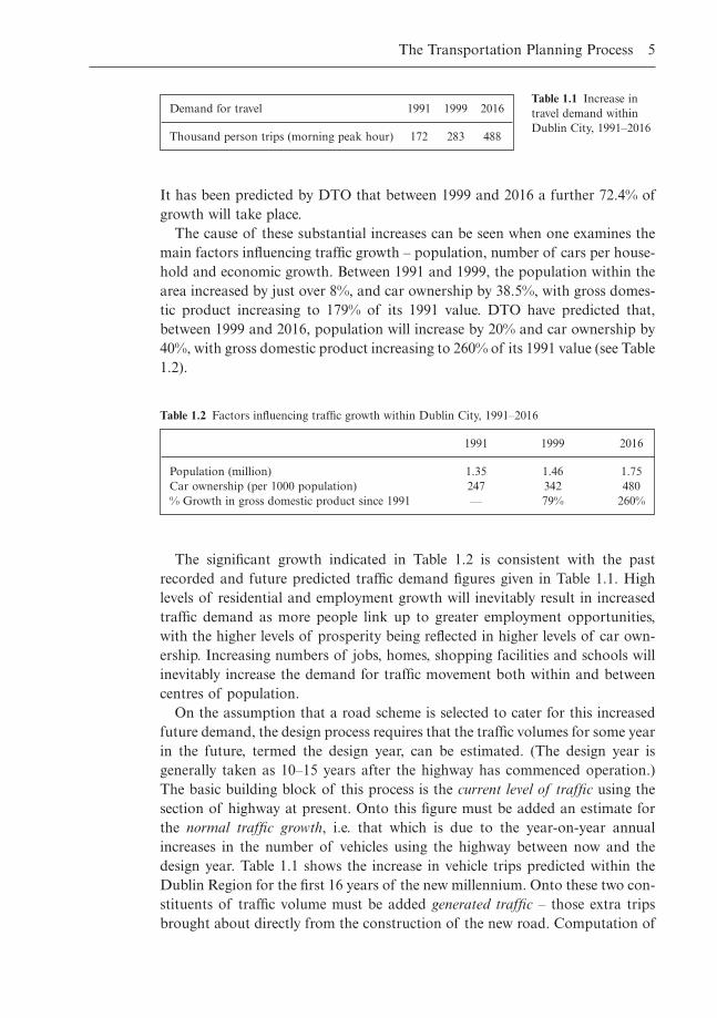
It has been predicted by DTO that between 1999 and 2016 a further 72.4% ofgrowth will take place.
The cause of these substantial increases can be seen when one examines themain factors influencing traffic growth – population, number of cars per house-hold and economic growth. Between 1991 and 1999, the population within thearea increased by just over 8%, and car ownership by 38.5%, with gross domes-tic product increasing to 179% of its 1991 value. DTO have predicted that,between 1999 and 2016, population will increase by 20% and car ownership by40%, with gross domestic product increasing to 260% of its 1991 value (see Table1.2).
The Transportation Planning Process 5
Demand for travel 1991 1999 2016
Thousand person trips (morning peak hour) 172 283 488
Table 1.1 Increase intravel demand withinDublin City, 1991–2016
1991 1999 2016
Population (million) 1.35 1.46 1.75Car ownership (per 1000 population) 247 342 480% Growth in gross domestic product since 1991 — 79% 260%
Table 1.2 Factors influencing traffic growth within Dublin City, 1991–2016
The significant growth indicated in Table 1.2 is consistent with the pastrecorded and future predicted traffic demand figures given in Table 1.1. Highlevels of residential and employment growth will inevitably result in increasedtraffic demand as more people link up to greater employment opportunities,with the higher levels of prosperity being reflected in higher levels of car own-ership. Increasing numbers of jobs, homes, shopping facilities and schools willinevitably increase the demand for traffic movement both within and betweencentres of population.
On the assumption that a road scheme is selected to cater for this increasedfuture demand, the design process requires that the traffic volumes for some yearin the future, termed the design year, can be estimated. (The design year is generally taken as 10–15 years after the highway has commenced operation.)The basic building block of this process is the current level of traffic using thesection of highway at present. Onto this figure must be added an estimate forthe normal traffic growth, i.e. that which is due to the year-on-year annualincreases in the number of vehicles using the highway between now and thedesign year. Table 1.1 shows the increase in vehicle trips predicted within theDublin Region for the first 16 years of the new millennium. Onto these two con-stituents of traffic volume must be added generated traffic – those extra tripsbrought about directly from the construction of the new road. Computation of
these three components enables the design-year volume of traffic to be estimatedfor the proposed highway. Within the design process, the design volume willdetermine directly the width of the travelled pavement required to deal with theestimated traffic levels efficiently and effectively.
1.4.3 Highway planning strategies
When the highway planning process takes place within a large urban area andother transport options such as rail and cycling may be under considerationalongside car-based ones, the procedure can become quite complex and theworkload involved in data collection can become immense. In such circum-stances, before a comprehensive study can be undertaken, one of a number ofbroad strategy options must be chosen:
� The land use transportation approach� The demand management approach� The car-centred approach� The public transport-centred approach.
Land use transportation approach
Within this method, the management of land use planning is seen as the solu-tion to controlling the demand for transport. The growing trend where manycommuters live in suburbs of a major conurbation or in small satellite townswhile working within or near the city centre has resulted in many using theirprivate car for their journey to work. This has led to congestion on the roadsand the need for both increased road space and the introduction of major publictransport improvements. Land use strategies such as the location of employ-ment opportunities close to large residential areas and actively limiting urbansprawl which tends to increase the dependency of commuters on the private car,are all viable land use control mechanisms.
The demand management approach
The demand management approach entails planning for the future by manag-ing demand more effectively on the existing road network rather than constructing new road links. Demand management measures include the tollingof heavily trafficked sections of highway, possibly at peak times only, and carpooling, where high occupancy rates within the cars of commuters is achievedvoluntarily either by the commuters themselves, in order to save money, or byemployers in order to meet some target stipulated by the planning authority.Use of car pooling can be promoted by allowing private cars with multiple occu-pants to use bus-lanes during peak hour travel or by allowing them reducedparking charges at their destination.
6 Highway Engineering
The car-centred approach
The car-centred approach has been favoured by a number of large cities withinthe US, most notably Los Angeles. It seeks to cater for future increases in trafficdemand through the construction of bigger and better roads, be they inter-urbanor intra-urban links. Such an approach usually involves prioritising the devel-opment of road linkages both within and between the major urban centres.Measures such as in-car information for drivers regarding points of congestionalong their intended route and the installation of state-of-the-art traffic controltechnology at all junctions, help maximise usage along the available road space.
The public transport-centred approach
In the public transport-centred approach the strategy will emphasise the impor-tance of bus and rail-based improvements as the preferred way of coping withincreased transport demand. Supporters of this approach point to the environ-mental and social advantages of such a strategy, reducing noise and air pollu-tion and increasing efficiency in the use of fossil fuels while also makingtransport available to those who cannot afford to run a car. However, the successof such a strategy depends on the ability of transport planners to induce increas-ing numbers of private car users to change their mode of travel during peak hours to public transport. This will minimise highway congestion as thenumber of peak hour journeys increase over the years. Such a result will onlybe achieved if the public transport service provided is clean, comfortable, regularand affordable.
1.4.4 Transportation studies
Whatever the nature of the proposed highway system under consideration, beit a new motorway to link two cities or a network of highway improvementswithin an urban centre, and whatever planning strategy the decision-makers areadopting (assuming that the strategy involves, to some extent, the constructionof new/upgraded roadways), a study must be carried out to determine the neces-sity or appropriateness of the proposal. This process will tend to be divided intotwo subsections:
� A transportation survey to establish trip-making patterns� The production and use of mathematical models both to predict future
transport requirements and to evaluate alternative highway proposals.
Transportation survey
Initially, the responsible transport planners decide on the physical boundarywithin which the study will take place. Most transport surveys have at their basis
The Transportation Planning Process 7
the land-use activities within the study area and involve making an inventory ofthe existing pattern of trip making, together with consideration of the socio-economic factors that affect travel patterns. Travel patterns are determined bycompiling a profile of the origin and destination (OD) of all journeys madewithin the study area, together with the mode of travel and the purpose of eachjourney. For those journeys originating within the study area, household surveysare used to obtain the OD information. These can be done with or without aninterviewer assisting. In the case of the former, termed a personal interviewsurvey, an interviewer records answers provided by the respondent. With thelatter, termed a self-completion survey, the respondent completes a question-naire without the assistance of an interviewer, with the usual format involvingthe questionnaire being delivered/mailed out to the respondent who then mailsit back/has it collected when all questions have been answered.
For those trips originating outside the study area, traversing its external‘cordon’ and ending within the study area, the OD information is obtained byinterviewing trip makers as they pass through the ‘cordon’ at the boundary ofthe study area. These are termed intercept surveys where people are interceptedin the course of their journey and asked where their trip started and where itwill finish.
A transportation survey should also gather information on the adequacy ofexisting infrastructure, the land use activities within the study area and detailson the socio-economic classification of its inhabitants. Traffic volumes along theexisting road network together with journey speeds, the percentage of heavygoods vehicles using it and estimates of vehicle occupancy rates are usuallyrequired. For each designated zone within the study area, office and factory floorareas and employment figures will indicate existing levels of industrial/commercial activity, while census information and recommendations on housingdensities will indicate population size. Some form of personal household-basedsurvey will be required within each zone to determine household incomes andtheir effect on the frequency of trips made and the mode of travel used.
Production and use of mathematical models
At this point, having gathered all the necessary information, models are devel-oped to translate the information on existing travel patterns and land-use pro-files into a profile of future transport requirements for the study area. The fourstages in constructing a transportation model are trip generation, trip distribu-tion, modal split and traffic assignment. The first stage estimates the number oftrips generated by each zone based on the nature and level of land-use activitywithin it. The second distributes these trips among all possible destinations, thusestablishing a pattern of trip making between each of the zones. The mode oftravel used by each trip maker to complete their journey is then determined andfinally the actual route within the network taken by the trip maker in each case.Each of these four stages is described in detail in the next chapter. Together they
8 Highway Engineering
form the process of transportation demand analysis which plays a central rolewithin highway engineering. It attempts to describe and explain both existingand future travel behaviour in an attempt to predict demand for both car-basedand other forms of transportation modes.
1.5 The decision-making process in highway and transport planning
1.5.1 Introduction
Highway and transportation planning can be described as a process of makingdecisions which concerns the future of a given transport system. The decisionsrelate to the determination of future demand; the relationships and interactionswhich exist between the different modes of transport; the effect of the proposedsystem on both existing land uses and those proposed for the future; the eco-nomic, environmental, social and political impacts of the proposed system andthe institutional structures in place to implement the proposal put forward.
Transport planning is generally regarded as a rational process, i.e. a rationaland orderly system for choosing between competing proposals at the planningstage of a project. It involves a combined process of information gathering anddecision-making.
The five steps in the rational planning process are summarised in Table 1.3.
The Transportation Planning Process 9
Step Purpose
Definition of goals and objectives To define and agree the overall purpose ofthe proposed transportation project
Formulation of criteria/measures of To establish standards of judging by whicheffectiveness the transportation options can be assessed in
relative and absolute termsGeneration of transportation alternatives To generate as broad a range of feasible
transportation options as possibleEvaluation of transportation alternatives To evaluate the relative merit of each
transportation optionSelection of preferred transportation To make a final decision on the adoption of
alternative/group of alternatives the most favourable transportation option asthe chosen solution for implementation
Table 1.3 Steps in the rational decision-making process for a transportation project
In the main, transport professionals and administrators subscribe to thevalues underlying rational planning and utilise this process in the form detailedbelow. The rational process is, however, a subset of the wider political decision-making system, and interacts directly with it both at the goal-setting stage andat the point in the process at which the preferred option is selected. In both situations, inputs from politicians and political/community groupings repre-
senting those with a direct interest in the transport proposal under scrutiny are essential in order to maximise the level of acceptance of the proposal under scrutiny.
Assuming that the rational model forms a central part of transport planningand that all options and criteria have been identified, the most important stagewithin this process is the evaluation/appraisal process used to select the mostappropriate transport option. Broadly speaking, there are two categories ofappraisal process. The first consists of a group of methods that require theassessments to be solely in money terms. They assess purely the economic consequences of the proposal under scrutiny. The second category consists of aset of more widely-based techniques that allow consideration of a wide rangeof decision criteria – environmental, social and political as well as economic,with assessments allowable in many forms, both monetary and non-monetary.The former group of methods are termed economic evaluations, with the lattertermed multi-criteria evaluations.
Evaluation of transport proposals requires various procedures to be followed.These are ultimately intended to clarify the decision relating to their approval.It is a vital part of the planning process, be it the choice between different loca-tion options for a proposed highway or the prioritising of different transportalternatives listed within a state, regional or federal strategy. As part of theprocess by which a government approves a highway scheme, in addition to thecarrying out of traffic studies to evaluate the future traffic flows that the pro-posed highway will have to cater for, two further assessments are of particularimportance to the overall approval process for a given project proposal:
� A monetary-based economic evaluation, generally termed a cost-benefitanalysis (CBA)
� A multi-criteria-based environmental evaluation, generally termed an environmental impact assessment (EIA)
Layered on top of the evaluation process is the need for public participationwithin the decision process. Although a potentially time consuming procedure, ithas the advantages of giving the planners an understanding of the public’s con-cerns regarding the proposal and also actively draws all relevant interest groupsinto the decision-making system. The process, if properly conducted, should serveto give the decision-makers some reassurance that all those affected by the devel-opment have been properly consulted before the construction phase proceeds.
1.5.2 Economic assessment
Within the US, both economic and environmental evaluations form a centralpart of the regional transportation planning process called for by federal lawwhen state level transportation plans required under the Intermodal Trans-portation Efficiency Act 1991 are being determined or in decisions by US federalorganisations regarding the funding of discretionary programmes.
10 Highway Engineering
Cost-benefit analysis is the most widely used method of project appraisalthroughout the world. Its origins can be traced back to a classic paper on theutility of public works by Dupuit (1844), written originally in the French language. The technique was first introduced in the US in the early part of thetwentieth century with the advent of the Rivers and Harbours Act 1902 whichrequired that any evaluation of a given development option must take explicitaccount of navigation benefits arising from the proposal, and these should beset against project costs, with the project only receiving financial support fromthe federal government in situations where benefits exceeded costs. Followingthis, a general primer, known as the ‘Green Book’, was prepared by the USFederal Interagency River Basin Committee (1950), detailing the general prin-ciples of economic analysis as they were to be applied to the formulation andevaluation of federally funded water resource projects. This formed the basis forthe application of cost-benefit analysis to water resource proposals, whereoptions were assessed on the basis of one criterion – their economic efficiency.In 1965 Dorfman released an extensive report applying cost-benefit analysis todevelopments outside the water resources sector. From the 1960s onwards thetechnique spread beyond the US and was utilised extensively to aid optionchoice in areas such as transportation.
Cost-benefit analysis is also widely used throughout Europe. The 1960s and 1970s witnessed a rapid expansion in the use of cost-benefit analysis withinthe UK as a tool for assessing major transportation projects. These studiesincluded the cost-benefit analysis for the London Birmingham Motorway by Coburn Beesley and Reynolds (1960) and the economic analysis for the sitingof the proposed third London airport by Flowerdew (1972). This growth was partly the result of the increased government involvement in the economyduring the post-war period, and partly the result of the increased size and complexity of investment decisions in a modern industrial state. The computerprogramme COBA has been used since the early 1980s for the economic assess-ment of major highway schemes (DoT, 1982). It assesses the net value of a pre-ferred scheme and can be used for determining the priority to be assigned to aspecific scheme, for generating a shortlist of alignment options to be presentedto local action groups for consultation purposes, or for the basic economic jus-tification of a given corridor. In Ireland, the Department of Finance requiresthat all highway proposals are shown to have the capability of yielding aminimum economic return on investment before approval for the scheme will begranted.
Detailed information on the economic assessment of highway schemes isgiven in Chapter 3.
1.5.3 Environmental assessment
Any economic evaluation for a highway project must be viewed alongside itsenvironmental and social consequences. This area of evaluation takes place
The Transportation Planning Process 11
within the environmental impact assessment (EIA) for the proposal. Within theUS, EIA was brought into federal law under the National Environmental PolicyAct 1969 which required an environmental assessment to be carried out in thecase of all federally funded projects likely to have a major adverse effect on thequality of the human environment. This law has since been imposed at statelevel also.
Interest in EIA spread from America to Europe in the 1970s in response tothe perceived deficiencies of the then existing procedures for appraising the envi-ronmental consequences of major development projects. The central importanceof EIA to the proper environmental management and the prevention of pollu-tion led to the introduction of the European Union Directive 85/337/EEC(Council of the European Communities, 1985) which required each memberstate to carry out an environmental assessment for certain categories of projects,including major highway schemes. Its overall purpose was to ensure that a mech-anism was in place for ensuring that the environmental dimension is properlyconsidered within a formal framework alongside the economic and technicalaspects of the proposal at its planning stage.
Within the UK, the environmental assessment for a highway proposal requires12 basic impacts to be assessed, including air, water and noise quality, landscape,ecology and land use effects, and impacts on culture and local communities,together with the disruption the scheme will cause during its construction. Therelative importance of the impacts will vary from one project to another. Thedetails of how the different types of impacts are measured and the format withinwhich they are presented are given in Chapter 3.
1.5.4 Public consultation
For major trunk road schemes, public hearings are held in order to give inter-ested parties an opportunity to take part in the process of determining both thebasic need for the highway and its optimum location.
For federally funded highways in the US, at least one public hearing will berequired if the proposal is seen to:
� Have significant environmental, social and economic effects� Require substantial wayleaves/rights-of-way, or� Have a significantly adverse effect on property adjoining the proposed
highway.
Within the hearing format, the state highway agency representative puts forwardthe need for the proposed roadway, and outlines its environmental, social andeconomic impacts together with the measures put forward by them to mitigate,as far as possible, these effects. The agency is also required to take submissionsfrom the public and consult with them at various stages throughout the projectplanning process.
12 Highway Engineering
Within the UK, the planning process also requires public consultation. Oncethe need for the scheme has been established, the consultation process centreson selecting the preferred route from the alternatives under scrutiny. In situa-tions where only one feasible route can be identified, public consultation willstill be undertaken in order to assess the proposal relative to the ‘do-minimum’option. As part of the public participation process, a consultation documentexplaining the scheme in layman’s terms and giving a broad outline of its costand environmental/social consequences, is distributed to all those with a legitimate interest in the proposal. A prepaid questionnaire is usually includedwithin the consultation document, which addresses the public’s preferencesregarding the relative merit of the alternative alignments under examination.In addition, an exhibition is held at all local council offices and public librariesat which the proposal is on public display for the information of those living in the vicinity of the proposal. Transport planners are obliged to take accountof the public consultation process when finalising the chosen route for the pro-posed motorway. At this stage, if objections to this route still persist, a publicenquiry is usually required before final approval is obtained from the secretaryof state.
In Ireland, two public consultations are built into the project managementguidelines for a major highway project. The first takes place before any alter-natives are identified and seeks to involve the public at a preliminary stage inthe scheme, seeking their involvement and general understanding. The secondpublic consultation involves presentation of the route selection study and therecommended route, together with its likely impacts. The views and reactions ofthe public are recorded and any queries responded to. The route selection reportis then reviewed in order to reflect any legitimate concerns of the public. Herealso, the responsible government minister may determine that a public inquiryis necessary before deciding whether or not to grant approval for the proposedscheme.
1.6 Summary
Highway engineering involves the application of scientific principles to the plan-ning, design, maintenance and operation of a highway project or system of pro-jects. The aim of this book is to give students an understanding of the analysisand design techniques that are fundamental to the topic. To aid this, numericalexamples are given throughout the book. This chapter has briefly introduced thecontext within which highway projects are undertaken, and details the frame-works, both institutional and procedural, within which the planning, design,construction and management of highway systems take place. The remainder of the chapters deal specifically with the basic technical details relating to theplanning, design, construction and maintenance of schemes within a highwaynetwork.
The Transportation Planning Process 13
Chapter 2 deals in detail with the classic four-stage model used to determinethe volume of flow on each link of a new or upgraded highway network. Theprocess of scheme appraisal is dealt with in Chapter 3, outlining in detailmethodologies for both economic and environmental assessment and illustrat-ing the format within which both these evaluations can be analysed. Chapter 4demonstrates how the twin factors of predicted traffic volume and level ofservice to be provided by the proposed roadway determine the physical size andnumber of lanes provided. Chapter 5 details the basic design procedures for thethree different types of highway intersections – priority junctions, roundaboutsand signalised intersections. The fundamental principles of geometric design,including the determination of both vertical and horizontal alignments, aregiven in Chapter 6. Chapter 7 summarises the basic materials which compriseroad pavements, both flexible and rigid, and outlines their structural properties,with Chapter 8 addressing details of their design and Chapter 9 dealing withtheir maintenance.
1.7 References
Coburn, T.M., Beesley, M.E. & Reynolds, D.J. (1960) The London-Birmingham Motor-way: Traffic and Economics. Technical Paper No. 46. Road Research Laboratory,Crowthorne.
Council of the European Communities (1985) On the assessment of the effects of certainpublic and private projects on the environment. Official Journal L175, 28.5.85, 40–48(85/337/EEC).
DoT (1982) Department of Transport COBA: A method of economic appraisal of highwayschemes. The Stationery Office, London.
Dupuit, J. (1844) On the measurement of utility of public works. International EconomicPapers, Volume 2.
Flowerdew, A.D.J. (1972) Choosing a site for the third London airport: The Roskill Commission approach. In R. Layard (ed.) Cost-Benefit Analysis. Penguin, London.
US Federal Interagency River Basin Committee (1950) Subcommittee on Benefits andCosts. Proposed Practices for Economic Analysis of River Basin Projects. WashingtonDC, USA.
14 Highway Engineering
Chapter 2
Forecasting Future Traffic Flows
2.1 Basic principles of traffic demand analysis
If transport planners wish to modify a highway network either by constructinga new roadway or by instituting a programme of traffic management improve-ments, any justification for their proposal will require them to be able to for-mulate some forecast of future traffic volumes along the critical links.Particularly in the case of the construction of a new roadway, knowledge of thetraffic volumes along a given link enables the equivalent number of standardaxle loadings over its lifespan to be estimated, leading directly to the design ofan allowable pavement thickness, and provides the basis for an appropriate geo-metric design for the road, leading to the selection of a sufficient number ofstandard width lanes in each direction to provide the desired level of service tothe driver. Highway demand analysis thus endeavours to explain travel behav-iour within the area under scrutiny, and, on the basis of this understanding,to predict the demand for the highway project or system of highway servicesproposed.
The prediction of highway demand requires a unit of measurement for travelbehaviour to be defined. This unit is termed a trip and involves movement froma single origin to a single destination. The parameters utilised to detail the natureand extent of a given trip are as follows:
� Purpose� Time of departure and arrival� Mode employed� Distance of origin from destination� Route travelled.
Within highway demand analysis, the justification for a trip is founded in eco-nomics and is based on what is termed the utility derived from a trip. An indi-vidual will only make a trip if it makes economic sense to do so, i.e. the economicbenefit or utility of making a trip is greater than the benefit accrued by not trav-elling, otherwise it makes sense to stay at home as travelling results in no eco-nomic benefit to the individual concerned. Utility defines the ‘usefulness’ ineconomic terms of a given activity. Where two possible trips are open to an indi-
vidual, the one with the greatest utility will be undertaken. The utility of anytrip usually results from the activity that takes place at its destination. Forexample, for workers travelling from the suburbs into the city centre by car, thebasic utility of that trip is the economic activity that it makes possible, i.e. thejob done by the traveller for which he or she gets paid. One must thereforeassume that the payment received by a given worker exceeds the cost of makingthe trip (termed disutility), otherwise it would have no utility or economic basis.The ‘cost’ need not necessarily be in money terms, but can also be the time takenor lost by the traveller while making the journey. If an individual can travel totheir place of work in more than one way, say for example by either car or bus,they will use the mode of travel that costs the least amount, as this will allowthem to maximise the net utility derived from the trip to their destination. (Netutility is obtained by subtracting the cost of the trip from the utility generatedby the economic activity performed at the traveller’s destination.)
2.2 Demand modelling
Demand modelling requires that all parameters determining the level of activ-ity within a highway network must first be identified and then quantified in orderthat the results output from the model has an acceptable level of accuracy. Oneof the complicating factors in the modelling process is that, for a given trip ema-nating from a particular location, once a purpose has been established formaking it, there are an enormous number of decisions relating to that trip, allof which must be considered and acted on simultaneously within the model.These can be classified as:
� Temporal decisions – once the decision has been made to make the journey,it still remains to be decided when to travel
� Decisions on chosen journey destination – a specific destination must beselected for the trip, e.g. a place of work, a shopping district or a school
� Modal decisions – relate to what mode of transport the traveller intends touse, be it car, bus, train or slower modes such as cycling/walking
� Spatial decisions – focus on the actual physical route taken from origin tofinal destination. The choice between different potential routes is made onthe basis of which has the shorter travel time.
If the modelling process is to avoid becoming too cumbersome, simplificationsto the complex decision-making processes within it must be imposed. Within abasic highway model, the process of simplification can take the form of twostages:
(1) Stratification of trips by purpose and time of day(2) Use of separate models in series for estimating the number of trips made
from a given geographical area under examination, the origin and desti-nation of each, the mode of travel used and the route selected.
16 Highway Engineering
Stratification entails modelling the network in question for a specific time of theday, most often the morning peak hour but also, possibly, some critical off-peakperiod, with trip purpose being stratified into work and non-work. For example,the modeller may structure the choice sequence where, in the first instance, allwork-related trips are modelled during the morning peak hour. (Alternatively,it may be more appropriate to model all non-work trips at some designated timeperiod during the middle of the day.) Four distinct traffic models are then usedsequentially, using the data obtained from the stratified grouping under scrutiny,in order to predict the movement of specific segments of the area’s populationat a specific time of day. The models are described briefly as:
� The trip generation model, estimating the number of trips made to and froma given segment of the study area
� The trip distribution model, estimating the origin and destination of eachtrip
� The modal choice model, estimating the form of travel chosen for each trip� The route assignment model, predicting the route selected for each trip.
Used in series, these four constitute what can be described as the basic traveldemand model. This sequential structure of traveller decisions constitutes a con-siderable simplification of the actual decision process where all decisions relatedto the trip in question are considered simultaneously, and it provides a sequenceof mathematical models of travel behaviour capable of meaningfully forecast-ing traffic demand.
An overall model of this type may also require information relating to theprediction of future land uses within the study area, along with projections ofthe socio-economic profile of the inhabitants, to be input at the start of the mod-elling process. This evaluation may take place within a land use study.
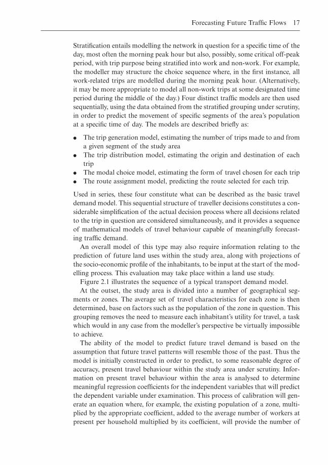
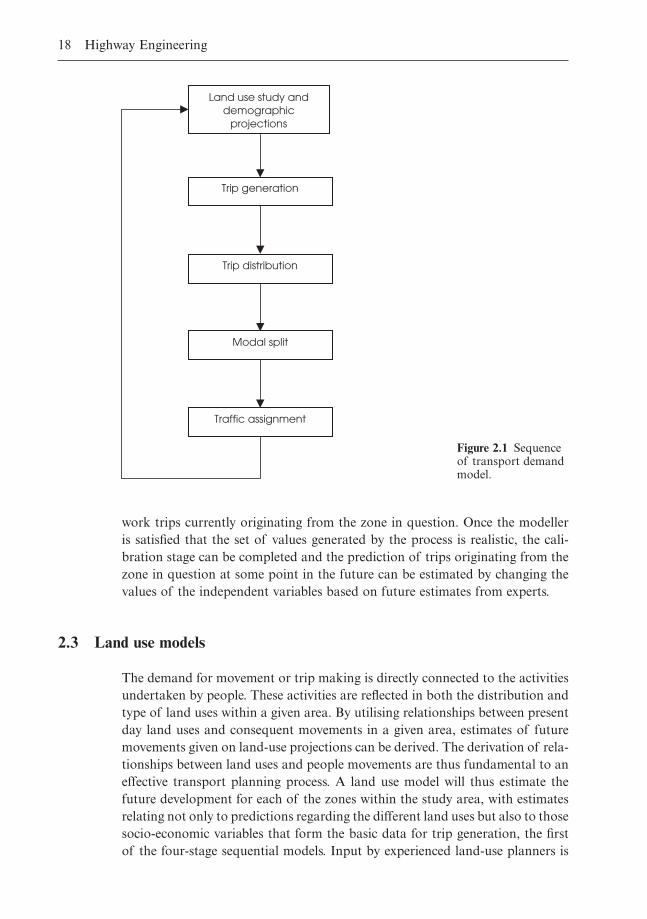
Figure 2.1 illustrates the sequence of a typical transport demand model.At the outset, the study area is divided into a number of geographical seg-
ments or zones. The average set of travel characteristics for each zone is thendetermined, base on factors such as the population of the zone in question. Thisgrouping removes the need to measure each inhabitant’s utility for travel, a taskwhich would in any case from the modeller’s perspective be virtually impossibleto achieve.
The ability of the model to predict future travel demand is based on theassumption that future travel patterns will resemble those of the past. Thus themodel is initially constructed in order to predict, to some reasonable degree ofaccuracy, present travel behaviour within the study area under scrutiny. Infor-mation on present travel behaviour within the area is analysed to determinemeaningful regression coefficients for the independent variables that will predictthe dependent variable under examination. This process of calibration will gen-erate an equation where, for example, the existing population of a zone, multi-plied by the appropriate coefficient, added to the average number of workers atpresent per household multiplied by its coefficient, will provide the number of
Forecasting Future Traffic Flows 17
work trips currently originating from the zone in question. Once the modelleris satisfied that the set of values generated by the process is realistic, the cali-bration stage can be completed and the prediction of trips originating from thezone in question at some point in the future can be estimated by changing thevalues of the independent variables based on future estimates from experts.
2.3 Land use models
The demand for movement or trip making is directly connected to the activitiesundertaken by people. These activities are reflected in both the distribution andtype of land uses within a given area. By utilising relationships between presentday land uses and consequent movements in a given area, estimates of futuremovements given on land-use projections can be derived. The derivation of rela-tionships between land uses and people movements are thus fundamental to aneffective transport planning process. A land use model will thus estimate thefuture development for each of the zones within the study area, with estimatesrelating not only to predictions regarding the different land uses but also to thosesocio-economic variables that form the basic data for trip generation, the firstof the four-stage sequential models. Input by experienced land-use planners is
18 Highway Engineering
Land use study and demographic
projections
Trip distribution
Modal split
Traffic assignment
Trip generation
Figure 2.1 Sequenceof transport demandmodel.
essential to the success of this phase. The end product of the land-use forecast-ing process usually takes the form of a land use plan where land-use estimatesstretching towards some agreed time horizon, usually between 5 and 25 years,are agreed.
The actual numerical relationship between land use and movement informa-tion is derived using statistical/mathematical techniques. A regression analysisis employed to establish, for a given zone within the study area, the relationshipbetween the vehicle trips produced by or attracted to it and characteristicsderived both from the land use study and demographic projections. This leadsus on directly to the first trip modelling stage – trip generation.
2.4 Trip generation
Trip generation models provide a measure of the rate at which trips both in andout of the zone in question are made. They predict the total number of tripsproduced by and attracted to its zone. Centres of residential development, wherepeople live, generally produce trips. The more dense the development and thegreater the average household income is within a given zone, the more trips willbe produced by it. Centres of economic activity, where people work, are the endpoint of these trips. The more office, factory and shopping space existing withinthe zone, the more journeys will terminate within it. These trips are 2-way excur-sions, with the return journey made at some later stage during the day.
It is an innately difficult and complex task to predict exactly when a trip willoccur. This complexity arises from the different types of trips that can be under-taken by a car user during the course of the day (work, shopping, leisure, etc.).The process of stratification attempts to simplify the process of predicting thenumber and type of trips made by a given zone. Trips are often stratified bypurpose, be it work, shopping or leisure. Different types of trips have differentcharacteristics that result in them being more likely to occur at different timesof the day. The peak time for the journey to work is generally in the earlymorning, while shopping trips are most likely during the early evening. Stratifi-cation by time, termed temporal aggregation, can also be used, where trip gen-eration models predict the number of trips per unit timeframe during any givenday. An alternative simplification procedure can involve considering the tripbehaviour of an entire household of travellers rather than each individual tripmaker within it. Such an approach is justified by the homogeneous nature, insocial and economic terms, of the members of a household within a given zone.
Within the context of an urban transportation study, three major variablesgovern the rate at which trips are made from each zone within the study area:
� Distance of zone from the central business district/city centre area� Socio-economic characteristics of the zone population (per capita income,
cars available per household)� Intensity of land use (housing units per hectare, employees per square metre
of office space).
Forecasting Future Traffic Flows 19
The relationships between trips generated and the relevant variables areexpressed as mathematical equations, generally in a linear form. For example,the model could take the following form:
(2.1)
whereTij = number of vehicle trips per time period for trip type i (work, non-work)
made by household jZ = characteristic value n for household j, based on factors such as the house-
hold income level and number of cars available within ita = regression coefficient estimated from travel survey data relating to n
A typical equation obtained for a transportation study in the UK might be:
whereT = total number of trips per household per 24 hoursZ1 = family sizeZ2 = total income of householdZ3 = cars per householdZ4 = housing density
T Z Z Z Z= + + + -0 0 07 0 005 0 95 0 0031 2 3 4. * . * . * . *
T Z Z Zij j j n nj= + + + +a a a a0 1 1 2 2 L
20 Highway Engineering
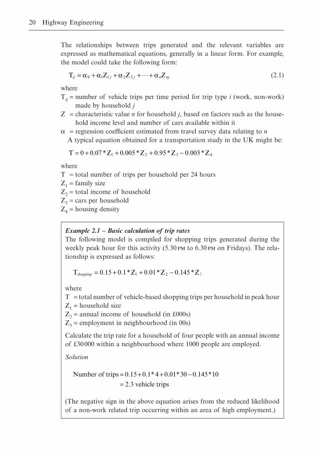
Example 2.1 – Basic calculation of trip ratesThe following model is compiled for shopping trips generated during theweekly peak hour for this activity (5.30 to 6.30 on Fridays). The rela-tionship is expressed as follows:
whereT = total number of vehicle-based shopping trips per household in peak hourZ1 = household sizeZ2 = annual income of household (in £000s)Z3 = employment in neighbourhood (in 00s)
Calculate the trip rate for a household of four people with an annual incomeof £30000 within a neighbourhood where 1000 people are employed.
Solution
(The negative sign in the above equation arises from the reduced likelihoodof a non-work related trip occurring within an area of high employment.)
Number of trips
vehicle trips
= + + -=
0 15 0 1 4 0 01 30 0 145 10
2 3
. . * . * . *
.
T Z Z Zshopping = + + -0 15 0 1 0 01 0 1451 2 3. . * . * . *
The coefficients a0 to an which occur within typical trip generation models asshown in equation 2.1 are determined through regression analysis. Manual solu-tions from multiple regression coefficients can be tedious and time-consumingbut software packages are readily available for solving them. For a given tripgeneration equation, the coefficients can be assumed to remain constant overtime for a given specified geographical location with uniform demographic andsocio-economic factors.
In developing such regression equations, among the main assumptions madeis that all the variables on the right-hand side of the equation are independentof each other. It may not, however, be possible for the transportation expert toconform to such a requirement and this may leave the procedure open to acertain level of criticism. In addition, basic errors in the regression equation mayexist as a result of biases or inaccuracies in the survey data from which it wasderived. Equation 2.1 assumes that the regression of the dependent variable onthe independent variables is linear, whereas in reality this may not be the case.
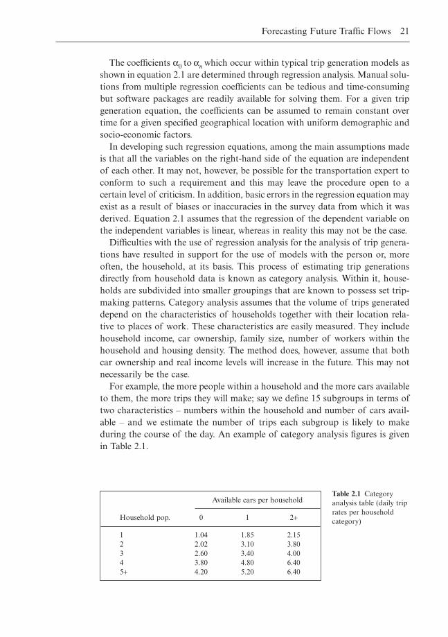
Difficulties with the use of regression analysis for the analysis of trip genera-tions have resulted in support for the use of models with the person or, moreoften, the household, at its basis. This process of estimating trip generationsdirectly from household data is known as category analysis. Within it, house-holds are subdivided into smaller groupings that are known to possess set trip-making patterns. Category analysis assumes that the volume of trips generateddepend on the characteristics of households together with their location rela-tive to places of work. These characteristics are easily measured. They includehousehold income, car ownership, family size, number of workers within thehousehold and housing density. The method does, however, assume that bothcar ownership and real income levels will increase in the future. This may notnecessarily be the case.
For example, the more people within a household and the more cars availableto them, the more trips they will make; say we define 15 subgroups in terms oftwo characteristics – numbers within the household and number of cars avail-able – and we estimate the number of trips each subgroup is likely to makeduring the course of the day. An example of category analysis figures is givenin Table 2.1.
Forecasting Future Traffic Flows 21
Available cars per household
Household pop. 0 1 2+
1 1.04 1.85 2.152 2.02 3.10 3.803 2.60 3.40 4.004 3.80 4.80 6.405+ 4.20 5.20 6.40
Table 2.1 Categoryanalysis table (daily triprates per householdcategory)

For the neighbourhood under examination, once the number of householdswithin each subgroup is established, the total number trips generated each daycan be calculated.
22 Highway Engineering
Example 2.2 – Calculating trip rates using category analysisFor a given urban zone, using the information on trip rates given in Table2.1 and the number of each household category within it as given in Table2.2, calculate the total number of daily trips generated by the 100 householdswithin the zone.
Solution
For each table cell, multiply the trip rate for each category by the number ofhouseholds in each category, summing all values to obtain a total number ofdaily trips as follows:
T = + + + + + ++ + + + + + + +
=
4 1 04 23 1 85 2 2 15 2 2 02 14 3 1 14 3 8 1 2 6
9 3 4 14 4 0 0 3 8 5 4 8 7 6 4 0 4 2 1 5 2 4 6 4
340 45
* . * . * . * . * . * . * .
* . * . * . * . * . * . * . * .
.
2.5 Trip distribution
2.5.1 Introduction
The previous model determined the number of trips produced by and attractedto each zone within the study area under scrutiny. For the trips produced by thezone in question, the trip distribution model determines the individual zoneswhere each of these will end. For the trips ending within the zone under exam-ination, the individual zone within which each trip originated is determined. Themodel thus predicts zone-to-zone trip interchanges. The process connects twoknown sets of trip ends but does not specify the precise route of the trip or themode of travel used. These are determined in the two last phases of the mod-elling process. The end product of this phase is the formation of a trip matrix
Household pop. Available cars per household
0 1 2+
1 4 23 22 2 14 143 1 9 144 0 5 75+ 0 1 4
Table 2.2 Categoryanalysis table (numberof households fromwithin zone in eachcategory, totalhouseholds = 100)
Forecasting Future Traffic Flows 23
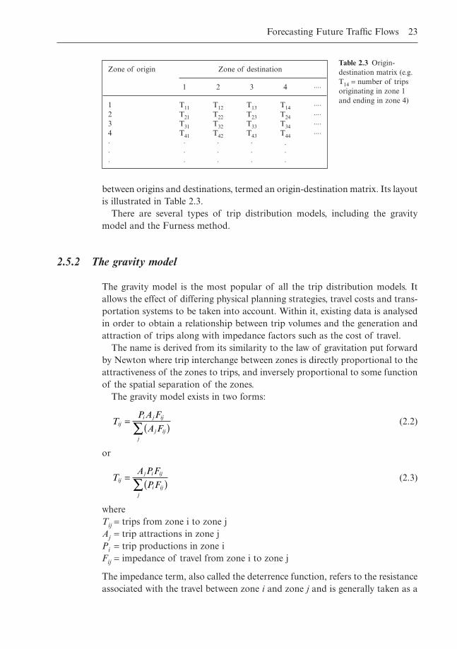
Zone of origin Zone of destination
1 2 3 4 ◊◊◊◊
1 T11 T12 T13 T14 ◊◊◊◊2 T21 T22 T23 T24 ◊◊◊◊3 T31 T32 T33 T34 ◊◊◊◊4 T41 T42 T43 T44 ◊◊◊◊◊ ◊ ◊ ◊ .◊ ◊ ◊ ◊ ◊◊ ◊ ◊ ◊ ◊
Table 2.3 Origin-destination matrix (e.g.T14 = number of tripsoriginating in zone 1and ending in zone 4)
between origins and destinations, termed an origin-destination matrix. Its layoutis illustrated in Table 2.3.
There are several types of trip distribution models, including the gravitymodel and the Furness method.
2.5.2 The gravity model
The gravity model is the most popular of all the trip distribution models. Itallows the effect of differing physical planning strategies, travel costs and trans-portation systems to be taken into account. Within it, existing data is analysedin order to obtain a relationship between trip volumes and the generation andattraction of trips along with impedance factors such as the cost of travel.
The name is derived from its similarity to the law of gravitation put forwardby Newton where trip interchange between zones is directly proportional to theattractiveness of the zones to trips, and inversely proportional to some functionof the spatial separation of the zones.
The gravity model exists in two forms:
(2.2)
or
(2.3)
whereTij = trips from zone i to zone jAj = trip attractions in zone jPi = trip productions in zone iFij = impedance of travel from zone i to zone j
The impedance term, also called the deterrence function, refers to the resistanceassociated with the travel between zone i and zone j and is generally taken as a
TA P F
P Fij
j i ij
i ijj
= ( )Â
TP A F
A Fij
i j ij
j ijj
= ( )Â
function of the cost of travel, travel time or travel distance between the twozones in question. One form of the deterrence function is:
Fij = C-aij (2.4)
The impedance function is thus expressed in terms of a generalised cost func-tion Cij and the a term which is a model parameter established either byanalysing the frequency of trips of different journey lengths or, less often, bycalibration.
Calibration is an iterative process within which initial values for Equation 2.4are assumed and Equation 2.2 or 2.3 is then calculated for known productions,attractions and impedances computed for the baseline year. The parameterswithin Equation 2.4 are then adjusted until a sufficient level of convergence isachieved.
24 Highway Engineering
Example 2.3 – Calculating trip distributions using the gravity modelTaking the information from an urban transportation study, calculate thenumber of trips from the central business zone (zone 1) to five other sur-rounding zones (zone 2 to zone 6).
Table 2.4 details the trips produced by and attracted to each of the sixzones, together with the journey times between zone 1 and the other fivezones.
Use Equation 2.2 to calculate the trip numbers. Within the impedancefunction, the generalised cost function is expressed in terms of the time takento travel between zone 1 and each of the other five zones and the model para-meter is set at 1.9.
Solution
Taking first the data for journeys between zone 1 and zone 2, the number ofjourneys attracted to zone 2, A2, is 45000. The generalised cost function forthe journey between the two zones is expressed in terms of the travel timebetween them: 5 minutes. Using the model parameter value of 1.9, the deter-rence function can be calculated as follows:
This value is then multiplied by A2:
Summing (Aj ¥ F1j) for j = 2Æ6 gives a value of 2114 (see Table 2.5)This value is divided into A2, and multiplied by the number of trips pro-
duced by zone 1 (P1) to yield the number of trips predicted to take place fromzone 1 to zone 2, i.e.
A F2 12 2114¥ =
F121 91 5 0 047= ∏ =( ). .
Contd
As illustrated by Equations 2.2 and 2.3, the gravity model can be used to dis-tribute either the productions from zone i or the attractions to zone j. If the cal-culation shown in Example 2.1 is carried out for the other five zones so that T2j,T3j, T4j, T5j and T6j are calculated, a trip matrix will be generated with the rowsof the resulting interchange matrix always summing to the number of trips pro-duced within each zone because of the form of Equation 2.2. However, thecolumns when summed will not give the correct number of trips attracted toeach zone. If, on the other hand, Equation 2.3 is used, the columns will sumcorrectly whereas the rows will not. In order to generate a matrix where row andcolumn values sum correctly, regardless of which model is used, an iterative cor-rection procedure, termed the row–column factor technique, can be used. Thistechnique is demonstrated in the final worked example in section 2. It isexplained briefly here.
Forecasting Future Traffic Flows 25
Example 2.3 Contd
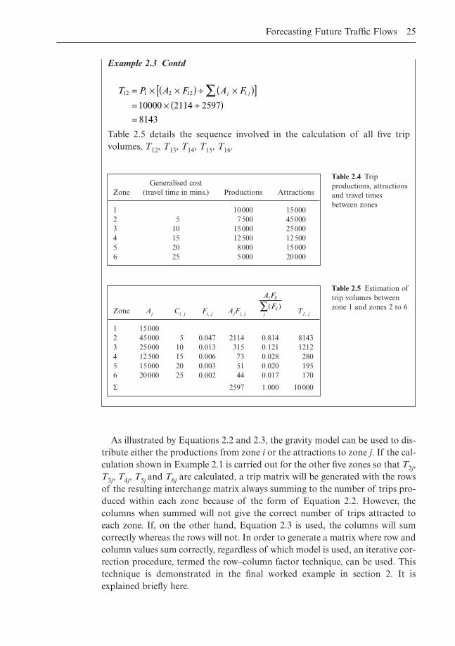
Table 2.5 details the sequence involved in the calculation of all five tripvolumes, T12, T13, T14, T15, T16.
T P A F A Fj j12 1 2 12 1
10000 2114 2597
8143
= ¥ ¥( ) ∏ ¥( )[ ]= ¥ ∏( )=
Â
Generalised costZone (travel time in mins.) Productions Attractions
1 10000 150002 5 7500 450003 10 15000 250004 15 12500 125005 20 8000 150006 25 5000 20000
Table 2.4 Tripproductions, attractionsand travel timesbetween zones
Zone Aj Ci, j Fi, j AjFi, j T1, j
1 150002 45000 5 0.047 2114 0.814 81433 25000 10 0.013 315 0.121 12124 12500 15 0.006 73 0.028 2805 15000 20 0.003 51 0.020 1956 20000 25 0.002 44 0.017 170
S 2597 1.000 10000
A FF
j ij
ijj
( )Â
Table 2.5 Estimation oftrip volumes betweenzone 1 and zones 2 to 6
Assuming Equation 2.2 is used, the rows will sum correctly but the columnswill not. The first iteration of the corrective procedure involves each value of Tijbeing modified so that each column will sum to the correct total of attractions.
(2.5)
Following this initial procedure, the rows will no longer sum correctly. There-fore, the next iteration involves a modification to each row so that they sum tothe correct total of trip productions.
(2.6)
This sequence of corrections is repeated until successive iterations result inchanges to values within the trip interchange matrix less than a specified per-centage, signifying that sufficient convergence has been obtained. If Equation2.3 is used, a similar corrective procedure is undertaken, but in this case theinitial iteration involves correcting the production summations.
2.5.3 Growth factor models
The cells within a trip matrix indicate the number of trips between each origin-destination pair. The row totals give the number of origins and the column totalsgive the number of destinations. Assuming that the basic pattern of traffic doesnot change, traffic planners may seek to update the old matrix rather thancompile a new one from scratch. The most straightforward way of doing this isby the application of a uniform growth factor where all cells within the existingmatrix are multiplied by the same value in order to generate an updated set offigures.
(2.7)
whereT t¢
ij = Trips from zone i to zone j in some future forecasted year t¢
T tij = Trips from zone i to zone j in the present year under observation t
Gtt¢ = Expected growth in trip volumes between year t and year t¢
One drawback of this approach lies in the assumption that all zones will growat the same rate. In reality, it is likely that some will grow at a faster rate thanothers. An approach that allows for such situations is the singly-constrainedgrowth factor approach, which can be applied to either origin or destinationdata, but not both. The former application is termed the origin constrainedgrowth factor method where a specific growth factor is applied to all trips orig-inating in zone i (see Equation 2.8 below), while the latter is termed the desti-
T T Gijt
ijt tt¢ ¢= ¥
¢ = ÂTP
Tij
i
iji
¢ = ÂTA
Tij
j
ijj
26 Highway Engineering
nation constrained growth factor method where a specific growth factor isapplied to all trips terminating in zone j (see Equation 2.9 below).
(2.8)
(2.9)
whereGtt¢
i = Expected growth in trip volumes between year t and year t¢ for trips withtheir origin in zone i (origins only)
Gtt¢j = Expected growth in trip volumes between year t and year t¢ for trips with
their destination in zone j (destinations only)
Where information exists on zone-specific growth factors for both origins anddestinations an average factor method can be applied where, for each origin-destination pair, the overall zone-specific growth factor is obtained from theaverage of the expected growth from origin i and destination j:
(2.10)
To obtain a more precise answer, however, a doubly constrained growth factormethod can be used. One of the most frequently used models of this type wasdevised by K.P. Furness (the Furness method).
2.5.4 The Furness method (Furness, 1965)
This again is a growth factor method, but in this instance the basic assumptionis that in the future the pattern of trip making will remain substantially identi-cal to those at present, with the trip volumes increasing in line with the growthof both the generating and attracting zones. It is still more straightforward thanthe gravity model and quite applicable to situations where substantial changesin external factors such as land use are not expected.
The basic information required in order to initiate this procedure can be sum-marised as:
DataT t
ij – The existing trip interchange matrix (in baseline year t)Oi – The total number of trips predicted to start from zone i in the future fore-
casted yearDj – The total number of trips predicted to terminate in zone j in the future
forecasted year.
To be computedTt¢
ij – The revised trip interchange matrix (in forecasted year t¢)Gtt¢
i – Origin growth factor for row i (growth between year t and year t¢)Gtt¢
j – Destination growth factor for column j (growth between year t and year t¢).
T TG G
ijt
ijt i
ttjtt
¢¢ ¢
= ¥+È
Î͢˚̇2
T T Gijt
ijt
jtt¢ ¢= ¥
T T Gijt
ijt
itt¢ ¢= ¥
Forecasting Future Traffic Flows 27
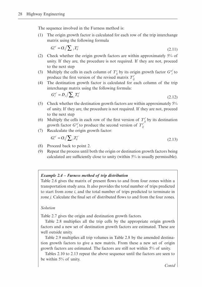
The sequence involved in the Furness method is:
(1) The origin growth factor is calculated for each row of the trip interchangematrix using the following formula
(2.11)
(2) Check whether the origin growth factors are within approximately 5% ofunity. If they are, the procedure is not required. If they are not, proceedto the next step
(3) Multiply the cells in each column of T tij by its origin growth factor Gtt¢
i toproduce the first version of the revised matrix Tt¢
ij(4) The destination growth factor is calculated for each column of the trip
interchange matrix using the following formula:
(2.12)
(5) Check whether the destination growth factors are within approximately 5%of unity. If they are, the procedure is not required. If they are not, proceedto the next step
(6) Multiply the cells in each row of the first version of Tt¢ij by its destination
growth factor Gtt¢i to produce the second version of Tt¢
ij(7) Recalculate the origin growth factor:
(2.13)
(8) Proceed back to point 2.(9) Repeat the process until both the origin or destination growth factors being
calculated are sufficiently close to unity (within 5% is usually permissible).
G O Titt
i j ijt¢ ¢= Â
G D Tjtt
ji
ijt¢ ¢= Â
G O Titt
i j ijt¢ = Â
28 Highway Engineering
Example 2.4 – Furness method of trip distributionTable 2.6 gives the matrix of present flows to and from four zones within atransportation study area. It also provides the total number of trips predictedto start from zone i, and the total number of trips predicted to terminate inzone j. Calculate the final set of distributed flows to and from the four zones.
Solution
Table 2.7 gives the origin and destination growth factors.Table 2.8 multiplies all the trip cells by the appropriate origin growth
factors and a new set of destination growth factors are estimated. These arewell outside unity.
Table 2.9 multiplies all trip volumes in Table 2.8 by the amended destina-tion growth factors to give a new matrix. From these a new set of origingrowth factors are estimated. The factors are still not within 5% of unity.
Tables 2.10 to 2.13 repeat the above sequence until the factors are seen tobe within 5% of unity.
Contd
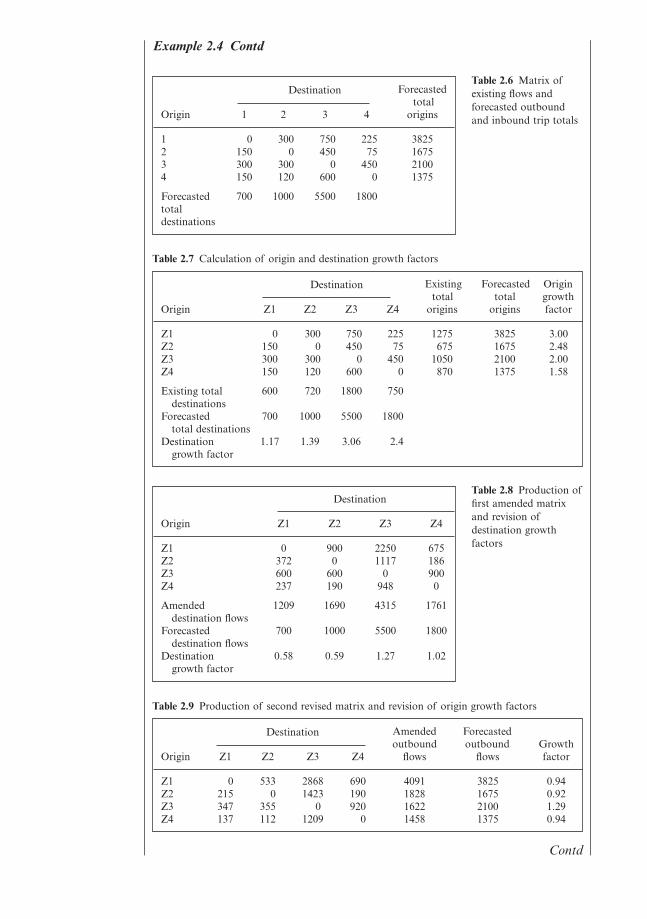
Example 2.4 Contd
ForecastedDestinationtotal
Origin 1 2 3 4 origins
1 0 300 750 225 38252 150 0 450 75 16753 300 300 0 450 21004 150 120 600 0 1375
Forecasted 700 1000 5500 1800totaldestinations
Table 2.6 Matrix ofexisting flows andforecasted outboundand inbound trip totals
Existing Forecasted OriginDestinationtotal total growth
Origin Z1 Z2 Z3 Z4 origins origins factor
Z1 0 300 750 225 1275 3825 3.00Z2 150 0 450 75 675 1675 2.48Z3 300 300 0 450 1050 2100 2.00Z4 150 120 600 0 870 1375 1.58
Existing total 600 720 1800 750destinations
Forecasted 700 1000 5500 1800total destinations
Destination 1.17 1.39 3.06 2.4growth factor
Table 2.7 Calculation of origin and destination growth factors
Destination
Origin Z1 Z2 Z3 Z4
Z1 0 900 2250 675Z2 372 0 1117 186Z3 600 600 0 900Z4 237 190 948 0
Amended 1209 1690 4315 1761destination flows
Forecasted 700 1000 5500 1800destination flows
Destination 0.58 0.59 1.27 1.02growth factor
Table 2.8 Production offirst amended matrixand revision ofdestination growthfactors
Contd
Amended ForecastedDestinationoutbound outbound Growth
Origin Z1 Z2 Z3 Z4 flows flows factor
Z1 0 533 2868 690 4091 3825 0.94Z2 215 0 1423 190 1828 1675 0.92Z3 347 355 0 920 1622 2100 1.29Z4 137 112 1209 0 1458 1375 0.94
Table 2.9 Production of second revised matrix and revision of origin growth factors
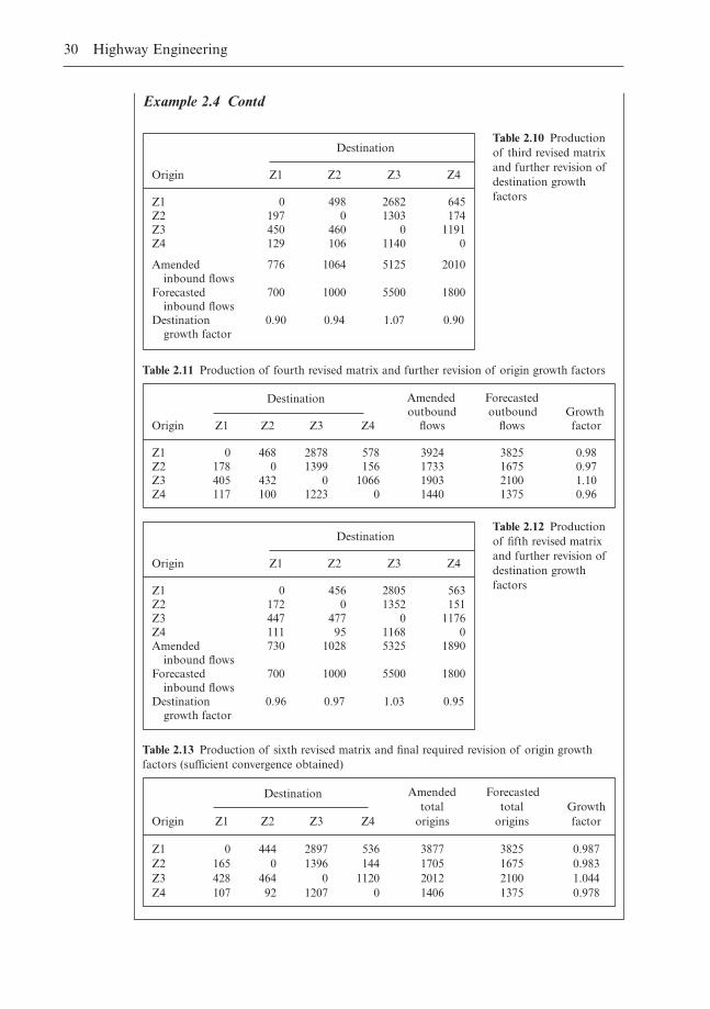
Example 2.4 Contd
30 Highway Engineering
Destination
Origin Z1 Z2 Z3 Z4
Z1 0 498 2682 645Z2 197 0 1303 174Z3 450 460 0 1191Z4 129 106 1140 0
Amended 776 1064 5125 2010inbound flows
Forecasted 700 1000 5500 1800inbound flows
Destination 0.90 0.94 1.07 0.90growth factor
Table 2.10 Productionof third revised matrixand further revision ofdestination growthfactors
Amended ForecastedDestinationoutbound outbound Growth
Origin Z1 Z2 Z3 Z4 flows flows factor
Z1 0 468 2878 578 3924 3825 0.98Z2 178 0 1399 156 1733 1675 0.97Z3 405 432 0 1066 1903 2100 1.10Z4 117 100 1223 0 1440 1375 0.96
Table 2.11 Production of fourth revised matrix and further revision of origin growth factors
Destination
Origin Z1 Z2 Z3 Z4
Z1 0 456 2805 563Z2 172 0 1352 151Z3 447 477 0 1176Z4 111 95 1168 0Amended 730 1028 5325 1890
inbound flowsForecasted 700 1000 5500 1800
inbound flowsDestination 0.96 0.97 1.03 0.95
growth factor
Table 2.12 Productionof fifth revised matrixand further revision ofdestination growthfactors
Amended ForecastedDestinationtotal total Growth
Origin Z1 Z2 Z3 Z4 origins origins factor
Z1 0 444 2897 536 3877 3825 0.987Z2 165 0 1396 144 1705 1675 0.983Z3 428 464 0 1120 2012 2100 1.044Z4 107 92 1207 0 1406 1375 0.978
Table 2.13 Production of sixth revised matrix and final required revision of origin growthfactors (sufficient convergence obtained)
The use of growth factor methods such as the Furness technique is, to a largeextent, dependent on the precise estimation of the actual growth factors used.These are a potential source of significant inaccuracy. The overriding drawbackof these techniques is the absence of any measure of travel impedance. Theycannot therefore take into consideration the effect of new or upgraded travelfacilities or the negative impact of congestion.
2.6 Modal split
Trips can be completed using different modes of travel. The proportion of tripsundertaken by each of the different modes is termed modal split. The simplestform of modal split is between public transport and the private car. While modalsplit can be carried out at any stage in the transportation planning process, it isassumed here to occur between the trip distribution and assignment phases. Thetrip distribution phase permits the estimation of journey times/costs for boththe public and private transport options. The modal split is then decided on the basis of these relative times/costs. In order to simplify the computation of modal split, journey time is taken as the quantitative measure of the cost criterion.
The decision by a commuter regarding choice of mode can be assumed tohave its basis in the micro-economic concept of utility maximisation. This modelpresupposes that a trip maker selects one particular mode over all others on thebasis that it provides the most utility in the economic sense. One must thereforebe in a position to develop an expression for the utility provided by any one ofa number of mode options. The function used to estimate the total utility pro-vided by a mode option usually takes the following form:
(2.14)
whereUm = total utility provided by mode option mbm = mode specific parameterzmj = set of travel characteristics of mode m, such as travel time or costsaj = parameters of the model, to be determined by calibration from travel
survey datae = stochastic term which makes allowance for the unspecifiable portion of
the utility of the mode that is assumed to be random
The bm terms state the relative attractiveness of different travel modes to thosewithin the market segment in question. They are understood to encapsulate theeffect of all the characteristics of the mode not incorporated within the z terms.The ‘e’ term expresses the variability in individual utilities around the averageutility of those within the market segment.
U zm m j mj= + +Âb a e
Forecasting Future Traffic Flows 31
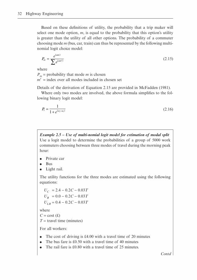
Based on these definitions of utility, the probability that a trip maker willselect one mode option, m, is equal to the probability that this option’s utilityis greater than the utility of all other options. The probability of a commuterchoosing mode m (bus, car, train) can thus be represented by the following multi-nomial logit choice model:
(2.15)
wherePm = probability that mode m is chosenm¢ = index over all modes included in chosen set
Details of the derivation of Equation 2.15 are provided in McFadden (1981).Where only two modes are involved, the above formula simplifies to the fol-
lowing binary logit model:
(2.16) P
e u u11
1 2 1=
+ -( )
Pe
em
um
um=
( )
¢( )Â
32 Highway Engineering
Example 2.5 – Use of multi-nomial logit model for estimation of modal splitUse a logit model to determine the probabilities of a group of 5000 workcommuters choosing between three modes of travel during the morning peakhour:
� Private car� Bus� Light rail.
The utility functions for the three modes are estimated using the followingequations:
UC = 2.4 - 0.2C - 0.03T
UB = 0.0 - 0.2C - 0.03T
ULR = 0.4 - 0.2C - 0.03T
whereC = cost (£)T = travel time (minutes)
For all workers:
� The cost of driving is £4.00 with a travel time of 20 minutes� The bus fare is £0.50 with a travel time of 40 minutes� The rail fare is £0.80 with a travel time of 25 minutes.
Contd
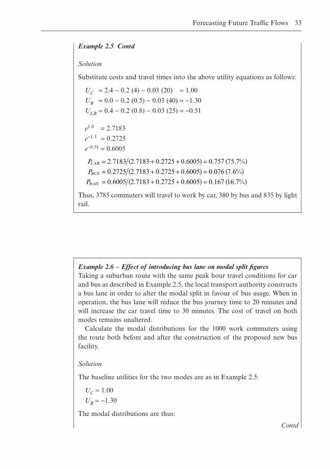
Forecasting Future Traffic Flows 33
Example 2.5 Contd
Solution
Substitute costs and travel times into the above utility equations as follows:
UC = 2.4 - 0.2 (4) - 0.03 (20) = 1.00
UB = 0.0 - 0.2 (0.5) - 0.03 (40) = -1.30
ULR = 0.4 - 0.2 (0.8) - 0.03 (25) = -0.51
e1.0 = 2.7183
e-1.3 = 0.2725
e-0.51 = 0.6005
Thus, 3785 commuters will travel to work by car, 380 by bus and 835 by lightrail.
P
P
P
CAR
BUS
RAIL
= + +( ) = ( )= + +( ) = ( )= + +( ) = ( )
2 7183 2 7183 0 2725 0 6005 0 757 75 7
0 2725 2 7183 0 2725 0 6005 0 076 7 6
0 6005 2 7183 0 2725 0 6005 0 167 16 7
. . . . . . %
. . . . . . %
. . . . . . %
Example 2.6 – Effect of introducing bus lane on modal split figuresTaking a suburban route with the same peak hour travel conditions for carand bus as described in Example 2.5, the local transport authority constructsa bus lane in order to alter the modal split in favour of bus usage. When inoperation, the bus lane will reduce the bus journey time to 20 minutes andwill increase the car travel time to 30 minutes. The cost of travel on bothmodes remains unaltered.
Calculate the modal distributions for the 1000 work commuters using the route both before and after the construction of the proposed new busfacility.
Solution
The baseline utilities for the two modes are as in Example 2.5:
UC = 1.00
UB = -1.30
The modal distributions are thus:
Contd
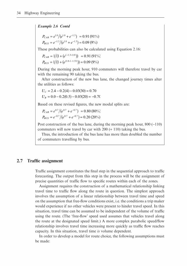
34 Highway Engineering
Example 2.6 Contd
These probabilities can also be calculated using Equation 2.16:
During the morning peak hour, 910 commuters will therefore travel by carwith the remaining 90 taking the bus.
After construction of the new bus lane, the changed journey times alterthe utilities as follows:
Based on these revised figures, the new modal splits are:
Post construction of the bus lane, during the morning peak hour, 800 (-110)commuters will now travel by car with 200 (+ 110) taking the bus.
Thus, the introduction of the bus lane has more than doubled the numberof commuters travelling by bus.
P e e e
P e e eCAR
BUS
= +( ) = ( )= +( ) = ( )
-
- -
0 7 0 7 0 7
0 7 0 7 0 7
0 80 80
0 20 20
. . .
. . .
. %
. %
U
UC
B
= - ( ) - ( ) == - ( ) - ( ) = -
2 4 0 2 4 0 03 30 0 70
0 0 0 2 0 5 0 03 20 0 70
. . . .
. . . . .
P e
P eCAR
BUS
= + ( )( ) = ( )= + ( )( ) = ( )
- -( )
- -( )( )
1 1 0 91 91
1 1 0 09 9
1 3 1 0
1 0 1 3
. .
. .
. %
. %
P e e e
P e e eCAR
BUS
= +( ) = ( )= +( ) = ( )
-
- -
1 0 1 0 1 3
1 3 1 0 1 3
0 91 91
0 09 9
. . .
. . .
. %
. %
2.7 Traffic assignment
Traffic assignment constitutes the final step in the sequential approach to trafficforecasting. The output from this step in the process will be the assignment ofprecise quantities of traffic flow to specific routes within each of the zones.
Assignment requires the construction of a mathematical relationship linkingtravel time to traffic flow along the route in question. The simplest approachinvolves the assumption of a linear relationship between travel time and speedon the assumption that free-flow conditions exist, i.e. the conditions a trip makerwould experience if no other vehicles were present to hinder travel speed. In thissituation, travel time can be assumed to be independent of the volume of trafficusing the route. (The ‘free-flow’ speed used assumes that vehicles travel alongthe route at the designated speed limit.) A more complex parabolic speed/flowrelationship involves travel time increasing more quickly as traffic flow reachescapacity. In this situation, travel time is volume dependent.
In order to develop a model for route choice, the following assumptions mustbe made:
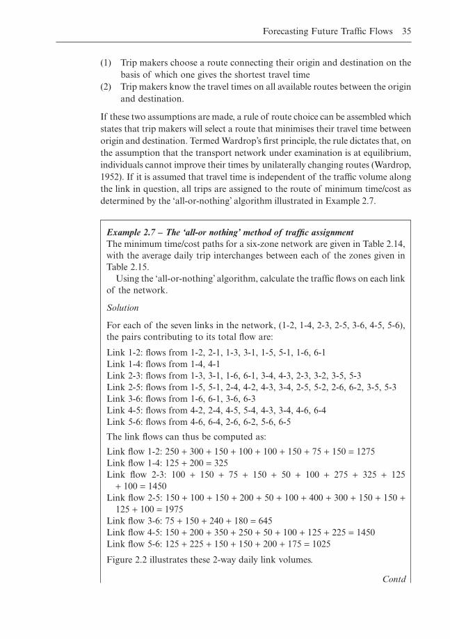
(1) Trip makers choose a route connecting their origin and destination on thebasis of which one gives the shortest travel time
(2) Trip makers know the travel times on all available routes between the originand destination.
If these two assumptions are made, a rule of route choice can be assembled whichstates that trip makers will select a route that minimises their travel time betweenorigin and destination. Termed Wardrop’s first principle, the rule dictates that, onthe assumption that the transport network under examination is at equilibrium,individuals cannot improve their times by unilaterally changing routes (Wardrop,1952). If it is assumed that travel time is independent of the traffic volume alongthe link in question, all trips are assigned to the route of minimum time/cost asdetermined by the ‘all-or-nothing’ algorithm illustrated in Example 2.7.
Forecasting Future Traffic Flows 35
Example 2.7 – The ‘all-or nothing’ method of traffic assignmentThe minimum time/cost paths for a six-zone network are given in Table 2.14,with the average daily trip interchanges between each of the zones given inTable 2.15.
Using the ‘all-or-nothing’ algorithm, calculate the traffic flows on each linkof the network.
Solution
For each of the seven links in the network, (1-2, 1-4, 2-3, 2-5, 3-6, 4-5, 5-6),the pairs contributing to its total flow are:
Link 1-2: flows from 1-2, 2-1, 1-3, 3-1, 1-5, 5-1, 1-6, 6-1Link 1-4: flows from 1-4, 4-1Link 2-3: flows from 1-3, 3-1, 1-6, 6-1, 3-4, 4-3, 2-3, 3-2, 3-5, 5-3Link 2-5: flows from 1-5, 5-1, 2-4, 4-2, 4-3, 3-4, 2-5, 5-2, 2-6, 6-2, 3-5, 5-3Link 3-6: flows from 1-6, 6-1, 3-6, 6-3Link 4-5: flows from 4-2, 2-4, 4-5, 5-4, 4-3, 3-4, 4-6, 6-4Link 5-6: flows from 4-6, 6-4, 2-6, 6-2, 5-6, 6-5
The link flows can thus be computed as:
Link flow 1-2: 250 + 300 + 150 + 100 + 100 + 150 + 75 + 150 = 1275Link flow 1-4: 125 + 200 = 325Link flow 2-3: 100 + 150 + 75 + 150 + 50 + 100 + 275 + 325 + 125
+ 100 = 1450Link flow 2-5: 150 + 100 + 150 + 200 + 50 + 100 + 400 + 300 + 150 + 150 +
125 + 100 = 1975Link flow 3-6: 75 + 150 + 240 + 180 = 645Link flow 4-5: 150 + 200 + 350 + 250 + 50 + 100 + 125 + 225 = 1450Link flow 5-6: 125 + 225 + 150 + 150 + 200 + 175 = 1025
Figure 2.2 illustrates these 2-way daily link volumes.
Contd
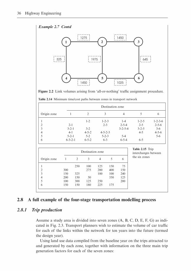
Example 2.7 Contd
2.8 A full example of the four-stage transportation modelling process
2.8.1 Trip production
Assume a study area is divided into seven zones (A, B, C, D, E, F, G) as indi-cated in Fig. 2.3. Transport planners wish to estimate the volume of car trafficfor each of the links within the network for ten years into the future (termedthe design year).
Using land use data compiled from the baseline year on the trips attracted toand generated by each zone, together with information on the three main tripgeneration factors for each of the seven zones:
36 Highway Engineering
1
4 65
321275 1450
1450 1025
1975325 645
Figure 2.2 Link volumes arising from ‘all-or-nothing’ traffic assignment procedure.
Destination zone
Origin zone 1 2 3 4 5 6
1 1-2 1-2-3 1-4 1-2-5 1-2-3-62 2-1 2-3 2-5-4 2-5 2-5-63 3-2-1 3-2 3-2-5-4 3-2-5 3-64 4-1 4-5-2 4-5-2-3 4-5 4-5-65 5-2-1 5-2 5-2-3 5-4 5-66 6-3-2-1 6-5-2 6-3 6-5-4 6-5
Table 2.14 Minimum time/cost paths between zones in transport network
Destination zone
Origin zone 1 2 3 4 5 6
1 250 100 125 150 752 300 275 200 400 1503 150 325 100 100 2404 200 150 50 350 1255 100 300 125 250 2006 150 150 180 225 175
Table 2.15 Tripinterchanges betweenthe six zones
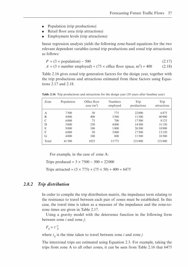
� Population (trip productions)� Retail floor area (trip attractions)� Employment levels (trip attractions)
linear regression analysis yields the following zone-based equations for the tworelevant dependent variables (zonal trip productions and zonal trip attractions)as follows:
P = (3 ¥ population) - 500 (2.17)A = (3 ¥ number employed) + (75 ¥ office floor space, m2) + 400 (2.18)
Table 2.16 gives zonal trip generation factors for the design year, together withthe trip productions and attractions estimated from these factors using Equa-tions 2.17 and 2.18.
Forecasting Future Traffic Flows 37
Zone Population Office floor Numbers Trip Triparea (m2) employed productions attractions
A 7500 50 775 22000 6475B 4000 400 3500 11500 40900C 6000 75 700 17500 8125D 5000 250 4000 14500 31150E 9000 100 1000 26500 10900F 6000 50 3000 17500 13150G 4000 100 800 11500 10300
Total 41500 1025 13775 121000 121000
Table 2.16 Trip productions and attractions for the design year (10 years after baseline year)
For example, in the case of zone A:
Trips produced = 3 ¥ 7500 - 500 = 22000
Trips attracted = (3 ¥ 775) + (75 ¥ 50) + 400 = 6475
2.8.2 Trip distribution
In order to compile the trip distribution matrix, the impedance term relating tothe resistance to travel between each pair of zones must be established. In thiscase, the travel time is taken as a measure of the impedance and the zone-to-zone times are given in Table 2.17.
Using a gravity model with the deterrence function in the following formbetween zone i and zone j:
Fij = t-2ij
where tij is the time taken to travel between zone i and zone j
The interzonal trips are estimated using Equation 2.3. For example, taking thetrips from zone A to all other zones, it can be seen from Table 2.16 that 6475
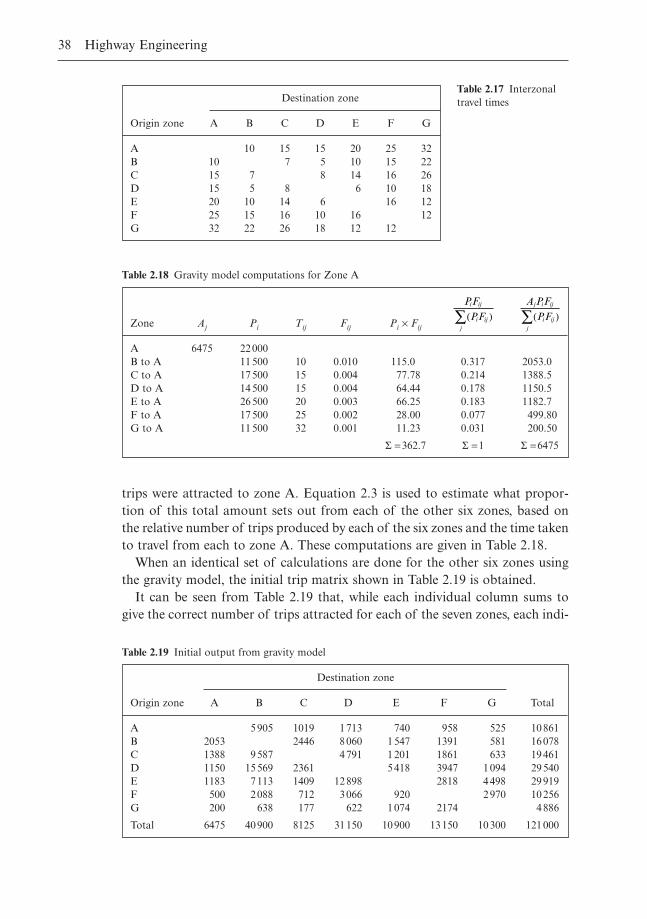
trips were attracted to zone A. Equation 2.3 is used to estimate what propor-tion of this total amount sets out from each of the other six zones, based onthe relative number of trips produced by each of the six zones and the time takento travel from each to zone A. These computations are given in Table 2.18.
When an identical set of calculations are done for the other six zones usingthe gravity model, the initial trip matrix shown in Table 2.19 is obtained.
It can be seen from Table 2.19 that, while each individual column sums togive the correct number of trips attracted for each of the seven zones, each indi-
38 Highway Engineering
Zone Aj Pi Tij Fij Pi ¥ Fij
A 6475 22000B to A 11500 10 0.010 115.0 0.317 2053.0C to A 17500 15 0.004 77.78 0.214 1388.5D to A 14500 15 0.004 64.44 0.178 1150.5E to A 26500 20 0.003 66.25 0.183 1182.7F to A 17500 25 0.002 28.00 0.077 499.80G to A 11500 32 0.001 11.23 0.031 200.50
S =362.7 S =1 S =6475
A PFPF
j i ij
i ijj
( )ÂPF
PFi ij
i ijj
( )Â
Table 2.18 Gravity model computations for Zone A
Destination zone
Origin zone A B C D E F G Total
A 5905 1019 1713 740 958 525 10861B 2053 2446 8060 1547 1391 581 16078C 1388 9587 4791 1201 1861 633 19461D 1150 15569 2361 5418 3947 1094 29540E 1183 7113 1409 12898 2818 4498 29919F 500 2088 712 3066 920 2970 10256G 200 638 177 622 1074 2174 4886
Total 6475 40900 8125 31150 10900 13150 10300 121000
Table 2.19 Initial output from gravity model
Destination zone
Origin zone A B C D E F G
A 10 15 15 20 25 32B 10 7 5 10 15 22C 15 7 8 14 16 26D 15 5 8 6 10 18E 20 10 14 6 16 12F 25 15 16 10 16 12G 32 22 26 18 12 12
Table 2.17 Interzonaltravel times
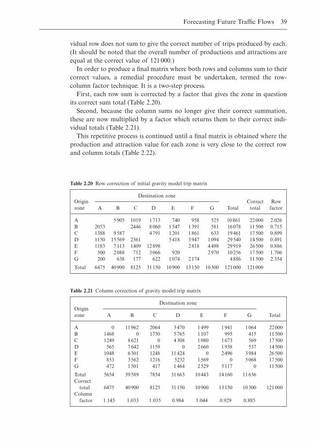
vidual row does not sum to give the correct number of trips produced by each.(It should be noted that the overall number of productions and attractions areequal at the correct value of 121000.)
In order to produce a final matrix where both rows and columns sum to theircorrect values, a remedial procedure must be undertaken, termed the row-column factor technique. It is a two-step process.
First, each row sum is corrected by a factor that gives the zone in questionits correct sum total (Table 2.20).
Second, because the column sums no longer give their correct summation,these are now multiplied by a factor which returns them to their correct indi-vidual totals (Table 2.21).
This repetitive process is continued until a final matrix is obtained where theproduction and attraction value for each zone is very close to the correct rowand column totals (Table 2.22).
Forecasting Future Traffic Flows 39
OriginDestination zone
Correct Rowzone A B C D E F G Total total factor
A 5 905 1019 1713 740 958 525 10861 22000 2.026B 2053 2446 8060 1547 1391 581 16078 11500 0.715C 1388 9587 4791 1201 1861 633 19461 17500 0.899D 1150 15569 2361 5418 3947 1094 29540 14500 0.491E 1183 7113 1409 12898 2818 4498 29919 26500 0.886F 500 2088 712 3066 920 2970 10256 17500 1.706G 200 638 177 622 1074 2174 4886 11500 2.354
Total 6475 40900 8125 31150 10900 13150 10300 121000 121000
Table 2.20 Row correction of initial gravity model trip matrix
OriginDestination zone
zone A B C D E F G Total
A 0 11962 2064 3470 1499 1941 1064 22000B 1468 0 1750 5765 1107 995 415 11500C 1249 8621 0 4308 1080 1673 569 17500D 565 7642 1159 0 2660 1938 537 14500E 1048 6301 1248 11424 0 2496 3984 26500F 853 3562 1216 5232 1569 0 5068 17500G 472 1501 417 1464 2529 5117 0 11500
Total 5654 39589 7854 31663 10443 14160 11636Correct
total 6475 40900 8125 31150 10900 13150 10300 121000Column
factor 1.145 1.033 1.035 0.984 1.044 0.929 0.885
Table 2.21 Column correction of gravity model trip matrix
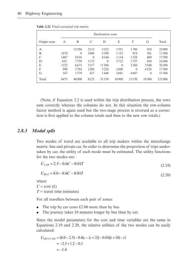
(Note, if Equation 2.2 is used within the trip distribution process, the rowssum correctly whereas the columns do not. In this situation the row-columnfactor method is again used but the two-stage process is reversed as a correc-tion is first applied to the column totals and then to the new row totals.)
2.8.3 Modal split
Two modes of travel are available to all trip makers within the interchangematrix: bus and private car. In order to determine the proportion of trips under-taken by car, the utility of each mode must be estimated. The utility functionsfor the two modes are:
(2.19)
(2.20)
whereC = cost (£)T = travel time (minutes)
For all travellers between each pair of zones:
� The trip by car costs £2.00 more than by bus� The journey takes 10 minutes longer by bus than by car.
Since the model parameters for the cost and time variables are the same in Equations 2.19 and 2.20, the relative utilities of the two modes can be easily calculated:
U c c t tBUS CAR-( ) = -( ) - - +( )( ) - +( ) -( )= - + -= -
0 0 2 5 0 6 2 0 01 10
2 5 1 2 0 1
1 4
. . . .
. . .
.
U C TBUS = - -0 0 0 6 0 01. . .
U C TCAR = - -2 5 0 6 0 01. . .
40 Highway Engineering
Destination zone
Origin zone A B C D E F G Total
A 12286 2112 3352 1551 1780 918 22000B 1670 0 1800 5599 1152 918 361 11500C 1407 8818 0 4144 1114 1528 489 17500D 632 7759 1172 0 2722 1757 458 14500E 1222 6673 1317 11380 0 2360 3548 26500F 998 3784 1286 5226 1680 0 4526 17500G 547 1579 437 1448 2681 4807 0 11500
Total 6475 40900 8125 31150 10900 13150 10300 121000
Table 2.22 Final corrected trip matrix
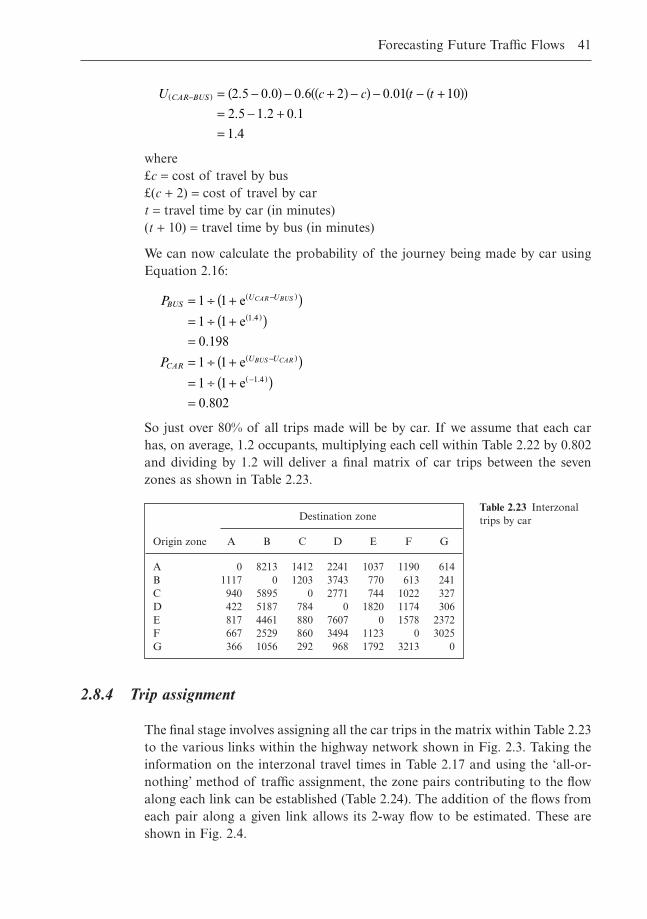
where£c = cost of travel by bus£(c + 2) = cost of travel by cart = travel time by car (in minutes)(t + 10) = travel time by bus (in minutes)
We can now calculate the probability of the journey being made by car usingEquation 2.16:
So just over 80% of all trips made will be by car. If we assume that each carhas, on average, 1.2 occupants, multiplying each cell within Table 2.22 by 0.802and dividing by 1.2 will deliver a final matrix of car trips between the sevenzones as shown in Table 2.23.
P
P
BUSU U
CARU U
CAR BUS
BUS CAR
= ∏ +( )= ∏ +( )== ∏ +( )= ∏ +( )=
-( )
( )
-( )
-( )
1 1
1 1
0 198
1 1
1 1
0 802
1 4
1 4
e
e
e
e
.
.
.
.
U c c t tCAR BUS-( ) = -( ) - +( ) -( ) - - +( )( )= - +=
2 5 0 0 0 6 2 0 01 10
2 5 1 2 0 1
1 4
. . . .
. . .
.
Forecasting Future Traffic Flows 41
Destination zone
Origin zone A B C D E F G
A 0 8213 1412 2241 1037 1190 614B 1117 0 1203 3743 770 613 241C 940 5895 0 2771 744 1022 327D 422 5187 784 0 1820 1174 306E 817 4461 880 7607 0 1578 2372F 667 2529 860 3494 1123 0 3025G 366 1056 292 968 1792 3213 0
Table 2.23 Interzonaltrips by car
2.8.4 Trip assignment
The final stage involves assigning all the car trips in the matrix within Table 2.23to the various links within the highway network shown in Fig. 2.3. Taking theinformation on the interzonal travel times in Table 2.17 and using the ‘all-or-nothing’ method of traffic assignment, the zone pairs contributing to the flowalong each link can be established (Table 2.24). The addition of the flows fromeach pair along a given link allows its 2-way flow to be estimated. These areshown in Fig. 2.4.
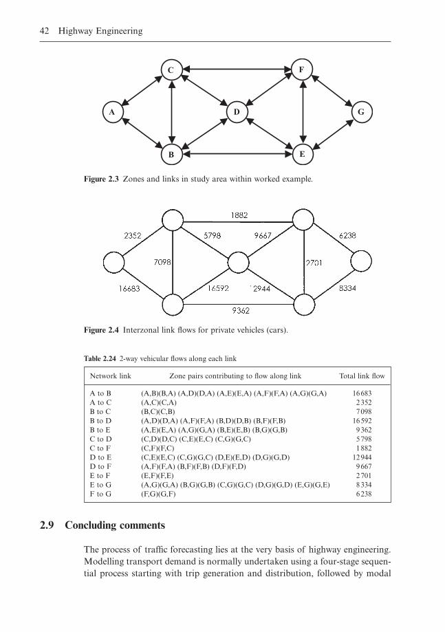
2.9 Concluding comments
The process of traffic forecasting lies at the very basis of highway engineering.Modelling transport demand is normally undertaken using a four-stage sequen-tial process starting with trip generation and distribution, followed by modal
42 Highway Engineering
C
B
A D
E
F
G
Figure 2.3 Zones and links in study area within worked example.
Figure 2.4 Interzonal link flows for private vehicles (cars).
Network link Zone pairs contributing to flow along link Total link flow
A to B (A,B)(B,A) (A,D)(D,A) (A,E)(E,A) (A,F)(F,A) (A,G)(G,A) 16683A to C (A,C)(C,A) 2352B to C (B,C)(C,B) 7098B to D (A,D)(D,A) (A,F)(F,A) (B,D)(D,B) (B,F)(F,B) 16592B to E (A,E)(E,A) (A,G)(G,A) (B,E)(E,B) (B,G)(G,B) 9362C to D (C,D)(D,C) (C,E)(E,C) (C,G)(G,C) 5798C to F (C,F)(F,C) 1882D to E (C,E)(E,C) (C,G)(G,C) (D,E)(E,D) (D,G)(G,D) 12944D to F (A,F)(F,A) (B,F)(F,B) (D,F)(F,D) 9667E to F (E,F)(F,E) 2701E to G (A,G)(G,A) (B,G)(G,B) (C,G)(G,C) (D,G)(G,D) (E,G)(G,E) 8334F to G (F,G)(G,F) 6238
Table 2.24 2-way vehicular flows along each link
split and concluding with traffic assignment. Predicting flows along the linkswithin a highway network provides vital information for the economic and envi-ronmental assessments required as part of the project appraisal process andallows the scale of each individual project within the network to be determined.Once the demand analysis and appraisal process have been completed, thedetailed junction and link design can then be undertaken.
It should be remembered, however, that the modelling process is a simplifi-cation of reality. Predictions arising from it are broad estimates rather thanprecise forecasts. The error range within which the model results are likely tofall should accompany any data supplied to the transport planners.
2.10 References
Furness, K.P. (1965) Time function iteration. Traffic Engineering Control, 7, 458–460.McFadden, D. (1981) Economic models and probabilistic choice. In Structural Analysis
of Discrete Data with Econometric Applications (eds Manski & McFadden). MIT Press,Cambridge, MA, USA.
Wardrop, J.G. (1952) Some theoretical aspects of road traffic research. Proceedings of theInstitution of Civil Engineers, 1(36), 325–362.
Forecasting Future Traffic Flows 43
Chapter 3
Scheme Appraisal for Highway Projects
3.1 Introduction
Once a transportation plan has been finalised and the demand along each of itshighway links has been established, a process must be put in place that helpsidentify the best solution for each individual proposal within the highwaynetwork. Each project must therefore be subject to an appraisal.
The aim of the highway appraisal process is therefore to determine the eco-nomic, societal and environmental feasibility of the project or group of projectsunder examination. The process enables highway planners to decide whether aproject is desirable in absolute terms and also provides a means of choosingbetween different competing project options, all of which have the ability to meetthe stated goals and objectives of the project sponsors.
The ‘reasoned choice’ model of individual or group decisions provides a decision-making framework within which scheme appraisal can take place,providing a technical foundation for non-recurring decisions such as the assess-ment of a highway construction/improvement proposal (Zey, 1992). It comprisesthe following steps:
(1) Problem recognition. The decision-maker determines that a problem existsand that a decision must be reflected on.
(2) Goal identification. The decision-maker details the desired result or out-come of the process.
(3) Identification of alternative highway schemes. Different potential solutionsare assembled prior to their evaluation.
(4) Information search. The decision-maker seeks to identify characteristicsassociated with the alternative solutions.
(5) Assessment of information on alternative highway schemes. The informationnecessary for making a decision regarding the preferred option is gatheredtogether and considered.
(6) Selection of preferred highway scheme. A preferred option is selected by thedecision-maker for implementation in the future.
(7) Evaluation. The decision is assessed a period of time after its implementa-tion in order to evaluate it on the basis of its achieved results.
Scheme Appraisal for Highway Projects 45
Clear rationality, where a judgement is arrived at following a sequence of delib-erately followed logical steps, lies at the basis of this model for decision-making.The principles of reasoned choice have been adapted into an analytic technique,called the rational approach, which has been detailed in Chapter 1.
The scheme appraisal process for highway schemes can be broken downbroadly into two sections: economic evaluation and environmental assessment.Background details of these two types of assessment have been given in Chapter1. Each of these is addressed in some detail below, and this chapter also dealswith an appraisal technique introduced in the UK that combines these two typesof highway project evaluation.
3.2 Economic appraisal of highway schemes
At various points in the development of a highway project, the developer willrequire economic assessments of the route options under consideration. Thiswill involve comparing their performance against the current situation, termedthe ‘do-nothing’ alternative, and/or against the ‘do-minimum’ alternative involv-ing a low-cost upgrading of the existing facility. Computations are performedon the costs and benefits associated with each highway option in order to obtainone or more measures of worth for each. Engineering economics provides anumber of techniques that result in numerical values termed measures of eco-nomic worth. These, by definition, consider the time value of money, an impor-tant concept in engineering economics that estimates the change in worth ofan amount of money over a given period of time. Some common measures ofworth are:
� Net present value (NPV)� Benefit/cost ratio (B/C)� Internal rate of return (IRR).
In economic analysis, financial units (pounds/euros/dollars) are used as the tan-gible basis of evaluation. With each of the above ‘measure of worth’ techniques,the fact that a quantity of money today is worth a different amount in the futureis central to the evaluation.
Within the process of actual selection of the best option in economic terms,some criterion based on one of the above measures of worth is used to selectthe chosen proposal. When several ways exist to accomplish a given objective,the option with the lowest overall cost or highest overall net income is chosen.While intangible factors that cannot be expressed in monetary terms do play apart in an economic analysis, their role in the evaluation is, to a large extent, asecondary one. If, however, the options available have approximately the sameequivalent cost/value, the non-economic and intangible factors may be used toselect the best option.
Economic appraisal techniques can be used to justify a scheme in absolute
46 Highway Engineering
terms, in which case the decision is made on the basis of whether the project is‘economically efficient’ or not. A negative net present value or a benefit/costratio less than unity would indicate an inefficient scheme where society wouldend up worse off with the scheme than without it. The economic benefits accru-ing to the beneficiaries of the highway would be exceeded by economic costsincurred by those ‘losing out’ as a result of its construction. In the main, thebeneficiaries are the road users and the ‘losers’ are those funding the scheme.Where the appraisal is being used to help differentiate between the economicperformances of competing options under examination, the scheme with thehighest measure of worth will be deemed the most efficient, assuming that atleast one will have a positive NPV or a B/C ratio greater than unity.
The framework within which this evaluation of the economic consequencesof highway schemes takes place is referred to as cost-benefit analysis.
3.3 Cost-benefit analysis (CBA)
3.3.1 Introduction
Within Europe, the method usually adopted for the economic evaluation ofhighway schemes, termed cost-benefit analysis, utilises the net present valuetechnique where the costs and benefits of the scheme are discounted over timeso that they represent present day values. Using this method, any proposalhaving a positive net present value is economically sustainable in absolute terms.Where competing project options are being compared, assuming they are beingused in identical capacities over the same period, the one with the numericallylarger NPV is selected (i.e. the one that is less negative or more positive). A briefhistorical background to the method has already been given in Chapter 1. Themain steps in the technique involve the listing of the main project options, theidentification and discounting to their present values of all relevant costs andbenefits required to assess them, and the use of economic indicators to enablea decision to be reached regarding the proposal’s relative or absolute desirabil-ity in economic terms.
3.3.2 Identifying the main project options
This is a fundamental step in the CBA process where the decision-makerscompile a list of all relevant feasible options that they wish to be assessed. It isusual to include a ‘do-nothing’ option within the analysis in order to gauge thoseevaluated against the baseline scenario where no work is carried out. The ‘do-minimum’ option offers a more realistic course of action where no new highwayis constructed but a set of traffic management improvements are made to theexisting route in order to improve the overall traffic performance. Evaluation of
Scheme Appraisal for Highway Projects 47
the ‘do-nothing’ scenario does however ensure that, in addition to the various‘live’ options being compared in relative terms, these are also seen to be eco-nomically justified in absolute terms, in other words their benefits exceed theircosts.
The term ‘feasible’ refers to options that, on a preliminary evaluation, presentthemselves as viable courses of action that can be brought to completion giventhe constraints imposed on the decision-maker such as lack of time, informa-tion and resources.
Finding sound feasible options is an important component of the decisionprocess. The quality of the final outcome can never exceed that allowed by thebest option examined. There are many procedures for both identifying anddefining project options. These include:
� Drawing on the personal experience of the decision-maker himself as wellas other experts in the highway engineering field
� Making comparisons between the current decision problem and ones previously solved in a successful manner
� Examining all relevant literature.
Some form of group brainstorming session can be quite effective in bringingviable options to light. Brainstorming consists of two main phases. Within thefirst, a group of people put forward, in a relaxed environment, as many ideas aspossible relevant to the problem being considered. The main rule for this phaseis that members of the group should avoid being critical of their own ideas orthose of others, no matter how far-fetched. This non-critical phase is very difficult for engineers, given that they are trained to think analytically or in ajudgmental mode (Martin, 1993). Success in this phase requires the engineer’sjudgmental mode to be ‘shut down’. This phase, if properly done, will result inthe emergence of a large number of widely differing options.
The second phase requires the planning engineer to return to normal judg-mental mode to select the best options from the total list, analysing each fortechnological, environmental and economic practicality. This is, in effect, ascreening process which filters through the best options. One such method is tocompare each new option with an existing, ‘tried-and-tested’ option used in pre-vious similar highway proposals by means of a T-chart (Riggs et al., 1997). Thechart contains a list of criteria which any acceptable option should satisfy. Theoption under examination is judged on the basis of whether it performs betteror worse than the conventional option on each of the listed criteria. It is vitalthat this process is undertaken by highway engineers with the appropriate levelof experience, professional training and local knowledge in order that a suffi-ciently wide range of options arise for consideration.
An example of a T-chart is shown in Table 3.1.In the example in Table 3.1, the proposed option would be rejected on the
basis that, while it had a lower construction cost, its maintenance costs and levelof environmental intrusion and geometric design, together with its low level of
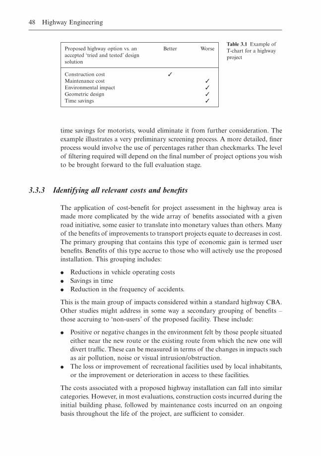
48 Highway Engineering
time savings for motorists, would eliminate it from further consideration. Theexample illustrates a very preliminary screening process. A more detailed, finerprocess would involve the use of percentages rather than checkmarks. The levelof filtering required will depend on the final number of project options you wishto be brought forward to the full evaluation stage.
3.3.3 Identifying all relevant costs and benefits
The application of cost-benefit for project assessment in the highway area ismade more complicated by the wide array of benefits associated with a givenroad initiative, some easier to translate into monetary values than others. Manyof the benefits of improvements to transport projects equate to decreases in cost.The primary grouping that contains this type of economic gain is termed userbenefits. Benefits of this type accrue to those who will actively use the proposedinstallation. This grouping includes:
� Reductions in vehicle operating costs� Savings in time� Reduction in the frequency of accidents.
This is the main group of impacts considered within a standard highway CBA.Other studies might address in some way a secondary grouping of benefits –those accruing to ‘non-users’ of the proposed facility. These include:
� Positive or negative changes in the environment felt by those people situatedeither near the new route or the existing route from which the new one willdivert traffic. These can be measured in terms of the changes in impacts suchas air pollution, noise or visual intrusion/obstruction.
� The loss or improvement of recreational facilities used by local inhabitants,or the improvement or deterioration in access to these facilities.
The costs associated with a proposed highway installation can fall into similarcategories. However, in most evaluations, construction costs incurred during theinitial building phase, followed by maintenance costs incurred on an ongoingbasis throughout the life of the project, are sufficient to consider.
Proposed highway option vs. an Better Worseaccepted ‘tried and tested’ designsolution
Construction cost ✓
Maintenance cost ✓
Environmental impact ✓
Geometric design ✓
Time savings ✓
Table 3.1 Example ofT-chart for a highwayproject
Scheme Appraisal for Highway Projects 49
The three primary user benefits listed above are normally estimated relativeto the without project or ‘do-nothing’ situation. The definition and descriptionof the without project scenario should be such that it constitutes an entirely feasible and credible course of action. Let us examine each of these benefits insome detail.
Reductions in vehicle operating costs
This constitutes the most direct potential benefit derived from a new orupgraded highway project. It is often the most important one and the one easiestto measure in money terms. While the users are the initial beneficiaries of thesepotential reductions, circumstances dictated by government policies or compe-tition, or the drive to maximise profits, might lead to other groups within thebroader community having a share in the ultimate benefit.
For a highway scheme, the new upgraded project leads to lower levels ofcongestion and higher speeds than on the existing roadway, usually resulting inlower fuel consumption and lower maintenance costs due to the reduced wearand tear on the vehicles.
Within a highway cost-benefit analysis, a formula is used which directly relatesvehicle-operating costs to speed. Costs included are both fuel and non-fuel-based. The higher speeds possible on the new road relative to the existing onelead to potential monetary savings for each road user.
Savings in time
The upgrading of a highway installation will invariably reduce travel time aswell as improving the reliability of transport services. For transport users, timehas some connection with money. The degree of correlation between the twodepends primarily on the manner in which the opportunities made possible bythe increased availability of time are utilised.
In general, analyses of the value of time-savings within the cost-benefit frame-work focus on distinguishing between travel for work and travel for non-workpurposes. Non-work time includes leisure travel and travel to and from work. Within developed economies, the value of working time is related to theaverage industrial wage plus added fringe benefits, on the assumption that timesaved will be diverted to other productive uses. There is no broad agreementamong economic evaluation experts regarding the valuation of non-work time. Since there is no direct market available that might provide the appro-priate value, values must be deduced from the choices members of the publicmake that involve differences in time. Studies carried out in industrialised coun-tries have indicated that travellers value non-working time at between 20% and35% the value attributed to working time (Adler, 1987). Less developed countries may, however, set the valuation at a lower percentage. In the workedexample presented in section 3.3.6, an average value for time savings is used
50 Highway Engineering
which supplies a single value covering both workers and non-workers using thehighway.
Reduction in the frequency of accidents
Assessing the economic benefit of accident reduction entails two steps. In thecase of a highway, this requires comparison of the accident rate on the existingunimproved highway with that of other highways elsewhere in the country (orabroad) constructed to the higher standard of the proposed new road. Normally,the higher the standard of construction of a highway, the lower its accident rate.
The second step involves the monetary valuation of the accident reduction.Three types of damage should be considered:
� Property damage� Personal injuries arising from serious accidents� Fatal accidents.
Property damage to vehicles involved in accidents is the most easily measuredin money terms. Reduced breakage of cargo can also be a significant benefit inproposed rail-based and seaport installations. Valuations can be obtaineddirectly from the extent of claims on insurance policies.
The cost of serious but non-fatal accidents is much more difficult to assess.Medical costs and the cost of lost output and personal pain and suffering con-stitute a large proportion of the total valuation.
There is major disagreement on which method is most appropriate for esti-mating the economic cost to society of a fatal accident. In recent times, statedpreference survey techniques have been employed to estimate this valuation.
In most cases, an average cost per accident, covering fatal and non-fatal, isemployed, with damage costs also accounted for within the final estimated value.
3.3.4 Economic life, residual value and the discount rate
A highway project is often complex and long term, with the costs and benefitsassociated with it occurring over a long time frame which we term the life of theproject, a parameter dealt with in earlier chapters. It sets a limit on the periodover which the costs and benefits are estimated, as all must occur within thistime slot, be it 25, 35 or even 50 years or more. It is related, in principle, to theexpected lifetime of the project under analysis.
Given that transport development projects have the potential to be in servicefor a very long time, it may seem impossible to set a limit on the life of theproject with any degree of certainty. In practice, however, this may not give riseto serious problems in the evaluation, as the loss of accuracy that results fromlimiting the life of a project to 35–40 years, instead of continuing the com-putation far beyond this point, is marginal to the analyst undertaking the evaluation. The shortened analysis can be justified on the basis that, in time
Scheme Appraisal for Highway Projects 51
equivalent terms, substantial costs and/or benefits are unlikely to arise in thelatter years of the project. If they are predicted, the life may well have to beextended. Truncating the analysis can also be justified on the basis of the un-certainty with which costs and benefits that occur beyond a certain time horizoncan be predicted.
Where this technique is applied after a relatively small number of years, theproject may well have to be assigned a substantial residual or salvage value,reflecting the significant benefits still to be accrued from the project or, con-versely, costs still liable to be incurred by it (a residual value can be negative, assay for a nuclear power station yet to be decommissioned). The difficulty inassigning a meaningful residual value to a project after so few years in com-mission results in this solution being rather unsatisfactory. It is far more advis-able to extend the evaluation to a future point in time where the residual valueis extremely small relative to its initial value.
In addition to this, the costs and benefits occur at different times over thistime horizon. Because of this, they cannot be directly combined until they arereduced to a common time frame. This is achieved using another parameterintroduced earlier, the discount rate, which translates all costs and benefits totime equivalent values. The actual value used is the social discount rate, giventhat the decision-maker is interested in the benefits and costs to society as awhole rather than to any individual or group of individuals.
The setting of this rate is quite a complex process, and is somewhat beyondthe scope of this text. It is important to point out, however, that it is not thesame as the market interest rate available to all private borrowers. It is a collec-tive discount rate reflecting a project of benefit to a large number of people andspanning a time frame greater than one full generation. A single definitive dis-count rate does not exist. Its estimation can be based on time preference or theopportunity cost of resources. The first is based on people in general having apreference for development taking place now rather than in the future. Becausethis involves taking a long-term view, the social time preference rate is usuallyset at a low, single-figure rate. The second reflects what members of society haveforegone as a result of funds being devoted to the development in question. Theprevailing real interest rate is often used as a guide for this value. Typical ratescan reach 15%, appreciably higher than the figure obtained from the time preference approach. Economists will have varying views about the most appro-priate test discount rate to use. In many instances the main decision-maker orthe person financing the proposal will set the rate. Before doing so, discussionswith all relevant stakeholders may be appropriate.
3.3.5 Use of economic indicators to assess basic economic viability
Once the two parameters of project life and discount rate are set in place,these allow all costs and benefits to be directly compared at the same point in
52 Highway Engineering
time. The decision-maker must now choose the actual mechanism for com-paring and analysing the costs and benefits in order to arrive at a final answer for the net benefit of each of the project options under consideration.Any of the three techniques listed earlier in the chapter can be used for thispurpose:
� Net present value (NPV)� Internal rate of return (IRR)� Benefit/cost ratio (B/C).
The NPV will estimate the economic worth of the project in terms of the presentworth of the total net benefits. The IRR will give, for each option under con-sideration, the rate at which the net present value for it equals zero, with the B/Cratio based on the ratio of the present value of the benefits to the present valueof the costs. For the last two methods, if the options under consideration aremutually exclusive, an incremental analysis must be carried out to establish thebest performing one in economic terms.
All three methods depend on discounting to arrive at a final answer. All,if used correctly, should give answers entirely consistent with each other, but the specific technique to be used varies with the circumstances. Thus, while the chosen technique is, to a certain extent, down to the preference of the decision-maker, it is nonetheless dependent on the type of decision to be taken within the analysis. If the decision is whether or not to proceed with agiven project, the result from the chosen technique is compared with some pre-determined threshold value in order to decide whether the project is economi-cally justified. Once a discount rate/minimum acceptable rate of return is set,any of the above methods will give the same result. Assuming a discount rateof 10%, the project will be economically acceptable if the NPV of the net ben-efits at 10% exceeds zero, if the IRR is above 10% or if the B/C ratio at 10%exceeds unity.
In the case of an independent project where choosing one does not excludethe possibility of proceeding with one or all of the others, all techniques yieldthe same result, the critical question being the choice of discount rate. In choos-ing between mutually exclusive projects where choice of one immediatelyexcludes all others, the most straightforward method involves choosing theoption with the maximum NPV of net benefits.
There may however be situations where it is required to rank order a numberof highway projects, on the basis that there is a set quantity of resources available for developing a certain category of project, and the decision-makerwishes to have a sequence in which these projects should be approved and constructed until the allotted resources are exhausted. In these cases, rankingbased on NPV may be of limited assistance, since high cost projects with slightlygreater NPV scores may be given priority over lower cost ones yielding greaterbenefits per unit cost. A correct course of action would be to rank the differentproject options based on their benefit/cost ratio, with the one with the highest
Scheme Appraisal for Highway Projects 53
B/C score given the rank 1, the second highest score given the rank 2, and soon.
Selecting a criterion for deciding between project options can be contentious.Some decision-makers are used to incorporating certain techniques in theiranalyses and are loath to change. IRR is rarely mentioned in the preceding para-graph, yet a number of national governments have a preference for it. This incli-nation towards it by some decision-makers is to some extent based on the factthat many have a background in banking and thus have an innate familiaritywith this criterion, together with the perception that its use does not require adiscount rate to be assumed or agreed. The latter statement is, in fact, incorrect,as, particularly when evaluating a single project, IRR must be compared withsome agreed discount rate.
Other supplementary methods of analysis such as cost effectiveness analysisand the payback period could also be used to analyse project options. Detailsof the payback method are given later in this chapter.
3.3.6 Highway CBA worked example
Introduction
It is proposed to upgrade an existing single carriageway road to a dual carriage-way and to improve some of the junctions. The time frame for construction ofthe scheme is set at two years, with the benefits of the scheme accruing to theroad users at the start of the third year. As listed above, the three main benefitsare taken as time savings, accident cost savings and vehicle operating cost reduc-tions. Construction costs are incurred mainly during the two years ofconstruction, but ongoing annual maintenance costs must be allowed forthroughout the economic life of the project, taken, in this case, to be 10 yearsafter the road has been commissioned.
The following basic data is assumed for this analysis:
Accident rates: 0.85 per million vehicle-kilometres (existing road)
0.25 per million vehicle-kilometres (upgraded road)
Average accident cost: £10000Average vehicle time savings: £2.00 per hourAverage vehicle speeds: 40km/h (existing road)
85km/h (upgraded road)Average vehicle operating cost: ((2 + (35/V) + 0.00005*V2) ∏ 100) £ per kmDiscount rate: 6%
The traffic flows and the construction/maintenance costs for the highway proposal are shown in Table 3.2.
54 Highway Engineering
Computation of discounted benefits and costs
Table 3.3 gives the valuations for the three user benefits over the 10 years of theupgraded highways operating life.
Year Predicted flow Construction cost Operating cost(106 v.km/yr) (£) (£)
1 — 15000000 —2 — 10000000 —3 250 — 5000004 260 — 5000005 270 — 5000006 280 — 5000007 290 — 5000008 300 — 5000009 310 — 500000
10 320 — 50000011 330 — 50000012 340 — 500000
Table 3.2 Traffic flowsand costs throughouteconomic life of thehighway proposal
Accident cost Operating Travel time Total user Discountedsavings cost savings savings benefits benefits
Year (£) (£) (£) (£) (£)
1 — — — — —2 — — — — —3 1500000 454963 6617647 8572610 71977294 1560000 473162 6882353 8915515 70619235 1620000 491360 7147059 9258419 69184296 1680000 509559 7411765 9601324 67685547 1740000 527757 7676471 9944228 66134808 1800000 545956 7941176 10287132 64542749 1860000 564155 8205882 10630037 6291902
10 1920000 582353 8470588 10972941 612723311 1980000 600552 8735294 11315846 596104612 2040000 618750 9000000 11658750 5794042
S =65188612
Table 3.3 Valuations of discounted highway user benefits
Taking the computations for year 7 as an example, the three individual userbenefits together with their total and discounted value are calculated as follows:
Accident savings (Yr 7) = (0.85 - 0.25) ¥ 10000 ¥ 290= £1740000
Operating cost (existing route) = (2 + 35/40 + (0.00005 ¥ 402)) ∏ 100= £0.02955 per km per vehicle
Operating cost (upgraded route) = (2 + 35/85 + (0.00005 ¥ 852)) ∏ 100= £0.02773 per km per vehicle
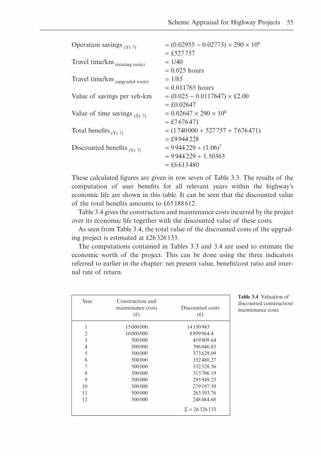
Scheme Appraisal for Highway Projects 55
Operation savings (Yr 7) = (0.02955 - 0.02773) ¥ 290 ¥ 106
= £527757Travel time/km (existing route) = 1/40
= 0.025 hoursTravel time/km (upgraded route) = 1/85
= 0.011765 hoursValue of savings per veh-km = (0.025 - 0.0117647) ¥ £2.00
= £0.02647Value of time savings (Yr 7) = 0.02647 ¥ 290 ¥ 106
= £7676471Total benefits (Yr 7) = (1740000 + 527757 + 7676471)
= £9944228Discounted benefits (Yr 7) = 9944229 ∏ (1.06)7
= 9944229 ∏ 1.50363= £6613480
These calculated figures are given in row seven of Table 3.3. The results of thecomputation of user benefits for all relevant years within the highway’s economic life are shown in this table. It can be seen that the discounted valueof the total benefits amounts to £65188612.
Table 3.4 gives the construction and maintenance costs incurred by the projectover its economic life together with the discounted value of these costs.
As seen from Table 3.4, the total value of the discounted costs of the upgrad-ing project is estimated at £26326133.
The computations contained in Tables 3.3 and 3.4 are used to estimate theeconomic worth of the project. This can be done using the three indicatorsreferred to earlier in the chapter: net present value, benefit/cost ratio and inter-nal rate of return.
Year Construction andmaintenance costs Discounted costs
(£) (£)
1 15000000 141509432 10000000 8899964.43 500000 419809.644 500000 396046.835 500000 373629.096 500000 352480.277 500000 332528.568 500000 313706.199 500000 295949.23
10 500000 279197.3911 500000 263393.7612 500000 248484.68
S = 26326133
Table 3.4 Valuation ofdiscounted construction/maintenance costs
56 Highway Engineering
Net present value
To obtain this figure, the discounted costs are subtracted from the discountedbenefits:
Benefit-cost ratio
In this case, the discounted benefits are divided by the discounted costs asfollows:
Internal rate of return
This measure of economic viability is estimated by finding the discount rate atwhich the discounted benefits equate with the discounted costs. In this example,this occurs at a rate of 28.1%.
Summary
All the above indicators point to the economic strength of the project underexamination. Its NPV at just over £38 million is strongly positive, and its B/Cratio at just below 2.5 is well in excess of unity. The IRR value of over 28% isover four times the agreed discount rate (6%). Together they give strong economic justification for the project under examination. Knowledge of theseindicators for a list of potential projects will allow decision-makers to comparethem in economic terms and to fast track those that deliver the maximum neteconomic benefit to the community.
3.3.7 COBA
Within the formal highway appraisal process in the UK for trunk roads, cost-benefit analysis is formally carried out using the COBA computer program(DoT, 1982) which assesses user costs and benefits over a 30-year period –assumed to be the useful life of the scheme – in order to obtain its net presentvalue. (The current version of the programme is COBA 9.) This is divided bythe initial capital cost of the scheme and expressed in percentage terms to givethe COBA rate of return.
The COBA framework involves comparing each alternative proposal with the ‘do-minimum’ option, with the resulting net costs and benefits providing
B C ratio = ∏=
65188 612 26 326133
2 476.
NPV = -=
65188 612 26 326133
38 862 479£
Scheme Appraisal for Highway Projects 57
the input to COBA. For example, if a choice is required between route A,route B and neither, then the costs and benefits of neither would be subtractedfrom each of the A and B valuations before the cost-benefit computation ismade.
The output from COBA is used to contribute to the following type ofdecision:
� To assess the need for improving a specific highway route. The improvementcould involve either the upgrading of an existing roadway or the construc-tion of a completely new one
� To determine what level of priority should be assigned to a particular schemeby considering its economic return relative to those of the other viableschemes in the area/region being considered by road administrators
� To determine the optimal timing of the scheme in question relative to otherroad schemes in the area
� To aid in the presentation of viable highway options to the public within aformal consultation process
� To establish optimal junction and link designs by comparing the economicperformance of the options under consideration.
The extent to which a full COBA analysis can be undertaken for a particularscheme depends on the stage reached in the assessment process, the data avail-able to the decision-maker and the nature of the decision to be taken. As thedesign procedure for a particular scheme advances, a more refined economicanalysis becomes possible.
Within COBA, in order to compute the three benefits accounted for withinthe procedure (savings in time, vehicle operating costs and accident costs) theprogram requires that the number of each category of vehicle utilising the linkunder examination throughout its economic life be determined using origin anddestination data gathered from traffic surveys.
The inputs to the COBA analysis are hugely dependent on the output of thetraffic forecasting and modelling process outlined in the previous chapter. Itassumes a fixed demand matrix of trips based on knowledge of existing flows and available traffic forecasts where travel demands in terms of origin and destinations and modes and times of travel remain unchanged. Thisassumption has the advantage of being relatively simple to apply and has beenused successfully for simple road networks. It has difficulty, however, in copingwith complex networks in urban areas or in situations where congestion is likely to occur on links directly affecting the particular scheme being assessed.This has a direct effect on the traffic assignment stage of the traffic modellingprocess, which is of central importance to the proper working of the COBA program. In the case of complex urban networks, where urban schemesresult in changes in travel behaviour that extend beyond simple reassignment oftrips, more complex models such as UREKA have been developed to predictflows.
58 Highway Engineering
3.3.8 Advantages and disadvantages of cost-benefit analysis
The final output from a cost-benefit analysis, in the opinion of Kelso (1964),should be a cardinal number representing the dollar rate of the streams of netprime benefits of the proposal that he termed ‘pure benefits’. Pure benefits mea-sured the net benefits with the project in relation to net benefits without theproject. Hill (1973) believed that this statement, one that explicitly sets out thebasis for a traditional cost-benefit analysis, reveals some of the major deficien-cies in the technique. Although there is some consideration of intangibles, theytend not to enter fully into the analysis. As a result, the effect of those invest-ments that can be measured in monetary terms, whether derived directly or indi-rectly from the market, are implicitly treated as being more important, for thesole reason that they are measurable in this way, when in reality the intangiblecosts and benefits may have more significant consequences for the proposal. Fur-thermore, cost-benefit analysis is most suitable for ranking or evaluating differ-ent highway options, rather than for testing the absolute suitability of a project.This is, to an extent, because all valuations of costs and benefits are subject toerror and uncertainty. Obtaining an absolute measure of suitability is an evengreater limitation.
The advantages and disadvantages of cost-benefit analysis can be summarisedas follows.
Advantages
� The use of the common unit of measurement, money, facilitates compar-isons between alternative highway proposals and hence aids the decision-making process.
� Given that the focus of the method is on benefits and costs of the highwayin question to the community as a whole, it offers a broader perspective thana narrow financial/investment appraisal concentrating only on the effects ofthe project on the project developers, be that the government or a group ofinvestors funding a toll scheme.
Disadvantages
� The primary basis for constructing a highway project may be a societal orenvironmental rather than an economic one. If the decision is based solelyon economic factors, however, an incorrect decision may result from the confusion of the original primary purpose of a proposed project with its secondary consequences, simply because the less important secondary consequences are measurable in money terms.
� The method is more suitable for comparing highway proposals designed tomeet a given transport objective, rather than evaluating the absolute desir-ability of one project in isolation. This is partly because all estimates of costs
Scheme Appraisal for Highway Projects 59
and benefits are subject to errors of forecasting. A decision-maker will thusfeel more comfortable using it to rank a number of alternative highwaydesign options, rather than to assess the absolute desirability of only oneoption relative to the existing ‘do-nothing’ situation, though this in somecases may be the only selection open to him/her.
� Although some limited recognition may be given to the importance of costsand benefits that cannot be measured in monetary terms, say, for example,the environmental consequences of the project in question, they tend to beneglected, or at best downgraded, within the main economic analysis. Thosegoods capable of measurement in monetary terms are usually attributedmore implicit importance even though, in terms of the overall viability ofthe project, they may be less significant.
The first two disadvantages can be managed effectively by employing an expe-rienced and competent decision expert to oversee use of the cost-benefit frame-work. Problems arising from the third point may require use of one of the othermethodologies detailed later in the chapter. Some efforts have been made toprovide monetary valuations for intangibles to enable their inclusion in cost-benefit. These techniques are in various stages of development.
3.4 Payback analysis
Payback analysis is an extremely simple procedure that is particularly useful inevaluating proposals such as privately funded highway projects where tolls willbe imposed on users of the facility in order to recover construction costs. Themethod delivers an estimate of the length of time taken for the project to recoupits construction costs. It does not require information on an appropriate inter-est rate, but the lack of accuracy of the method requires that results from itshould not be given the same weight as those from formal economic techniquesoutlined in this chapter, such as cost-benefit analysis. The method assumes thata given proposal will generate a stream of monies during its economic life, andat some point the total value of this stream will exactly equal its initial cost. Thetime taken for this equalisation to occur is called the payback period. It is moreusefully applied to projects where the timescale for equalisation is relativelyshort. The method itself does not address the performance of the proposal afterthe payback period. Its analysis is thus not as complete as the more formal tech-niques, and therefore its results, when taken in isolation, may be misleading. Itis therefore best utilised as a back-up technique, supplementing the informationfrom one of the more comprehensive economic evaluation methods.
While the method has certain shortcomings, it is utilised frequently by engi-neering economists. Its strength lies in its simplicity and basic logic. It addressesa question that is very important to the developer of a tolled highway facility,as a relatively speedy payback will protect liquidity and release funds more
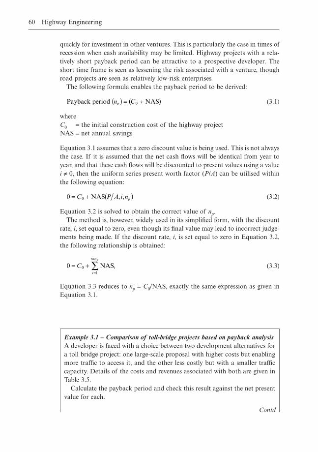
60 Highway Engineering
quickly for investment in other ventures. This is particularly the case in times ofrecession when cash availability may be limited. Highway projects with a rela-tively short payback period can be attractive to a prospective developer. Theshort time frame is seen as lessening the risk associated with a venture, thoughroad projects are seen as relatively low-risk enterprises.
The following formula enables the payback period to be derived:
(3.1)
whereC0 = the initial construction cost of the highway projectNAS = net annual savings
Equation 3.1 assumes that a zero discount value is being used. This is not alwaysthe case. If it is assumed that the net cash flows will be identical from year toyear, and that these cash flows will be discounted to present values using a valuei π 0, then the uniform series present worth factor (P/A) can be utilised withinthe following equation:
(3.2)
Equation 3.2 is solved to obtain the correct value of np.The method is, however, widely used in its simplified form, with the discount
rate, i, set equal to zero, even though its final value may lead to incorrect judge-ments being made. If the discount rate, i, is set equal to zero in Equation 3.2,the following relationship is obtained:
(3.3)
Equation 3.3 reduces to np = C0/NAS, exactly the same expression as given inEquation 3.1.
0 01
= +=
=
ÂC tt
t np
NAS
0 0= + ( )C P A i npNAS , ,
Payback period NASn Cp( ) = ∏( )0
Example 3.1 – Comparison of toll-bridge projects based on payback analysisA developer is faced with a choice between two development alternatives fora toll bridge project: one large-scale proposal with higher costs but enablingmore traffic to access it, and the other less costly but with a smaller trafficcapacity. Details of the costs and revenues associated with both are given inTable 3.5.
Calculate the payback period and check this result against the net presentvalue for each.
Contd
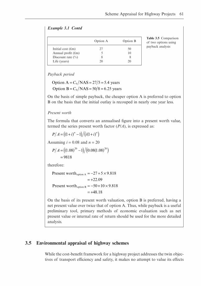
Scheme Appraisal for Highway Projects 61
Example 3.1 Contd
Payback period
On the basis of simple payback, the cheaper option A is preferred to optionB on the basis that the initial outlay is recouped in nearly one year less.
Present worth
The formula that converts an annualised figure into a present worth value,termed the series present worth factor (P/A), is expressed as:
Assuming i = 0.08 and n = 20
therefore:
On the basis of its present worth valuation, option B is preferred, having anet present value over twice that of option A. Thus, while payback is a usefulpreliminary tool, primary methods of economic evaluation such as netpresent value or internal rate of return should be used for the more detailedanalysis.
Present worth
Present worth
option A
option B
= - + ¥= += - + ¥= +
27 5 9 818
22 09
50 10 9 818
48 18
.
.
.
.
P A = ( ) -( ) ( )( )=
1 08 1 0 08 1 08
9818
20 20. . .
P A i i in n= +( ) -( ) +( )( )1 1 1
Option A NAS years
Option B NAS years
= = == = =
C
C0
0
27 5 5 4
50 8 6 25
.
.
Option A Option B
Initial cost (£m) 27 50Annual profit (£m) 5 10Discount rate (%) 8 8Life (years) 20 20
Table 3.5 Comparisonof two options usingpayback analysis
3.5 Environmental appraisal of highway schemes
While the cost-benefit framework for a highway project addresses the twin objec-tives of transport efficiency and safety, it makes no attempt to value its effects

62 Highway Engineering
on the environment. Environmental evaluation therefore requires an alternativeanalytical structure. The structure developed within the last 30 years is termedenvironmental impact assessment (EIA).
The procedure has its origins in the US during the 1960s when environmen-tal issues gained in importance. The legal necessity for public consultationduring the planning stage of a highways project, allied to the preoccupation with environmental issues by environmental groups, resulted in the identifiedneed for environmental assessment within the project planning process.The process was made statutory under the National Environmental Policy Act1969 which requires the preparation of an environmental impact statement(EIS) for any environmentally significant project undertaken by the federal government. NEPA prescribes a format for the EIS, requiring the developer to assess:
� The probable environmental impact of the proposal� Any unavoidable environmental impacts� Alternative options to the proposal� Short-run and long-run effects of the proposal and any relationship between
the two� Any irreversible commitment of resources necessitated by the proposal.
This list aids the identification and evaluation of all impacts relevant to the evaluation of the project concerned.
Interest in EIA spread to Europe during the 1970s in response to the per-ceived shortcomings within the then existing procedures for assessing the envi-ronmental consequences of large-scale development projects and for predictingthe long-term direct and indirect environmental and social effects. The advan-tages of such a procedure was noted by the European Commission, and the con-tribution of EIA to proper environmental management was noted in the SecondAction Programme on the Environment, published by them in 1977. A centralobjective of this programme was to put in place a mechanism for ensuring thatthe effects on the environment of development projects such as major highwayschemes would be taken into account at the earliest possible stages within theirplanning process. A directive (85/337/EEC) (Council of the European Commu-nities, 1985) giving full effect to these elements of European Union policy wasagreed and passed in July 1985 with the requirement that it be transposed intothe legislation of every member state within three years.
The directive helps ensure that adequate consideration is given to the envi-ronmental effects of a development project by providing a mechanism for ensur-ing that the environmental factors relevant to the project under examination areproperly considered within a formal statement – the EIS – structured alongbroadly the same lines as the US model.
The directive also details the minimum information that must be containedwithin the EIS. These include:
Scheme Appraisal for Highway Projects 63
(1) A physical description of the project(2) A description of measures envisaged to reduce/remedy the significant
adverse environmental effects of the project(3) The data required to both identify and assess the main effects on the envi-
ronment of the project in question.
Within the UK, since 1993 the Design Manual for Roads and Bridges (DoT,1993) has provided the format within which the environmental assessment ofhighway schemes has taken place. It identified 12 environmental impacts to beassessed for any new/improved trunk road proposal. These, together with theeconomic assessment, would form the decision-making framework used as thebasis both for choosing between competing options for a given highway routecorridor and for deciding in absolute terms whether the proposal in any formshould be proceeded with.
The 12 environmental impacts forming the assessment framework are:
� Air quality The main vehicle pollutants assessed are carbon monoxide(CO), oxides of nitrogen (NOX) and hydrocarbons (HC), lead (Pb), carbondioxide (CO2) and particulates. Established models are used to predict futurelevels of these pollutants, and the values obtained are compared with currentair quality levels.
� Cultural heritage The demolition/disturbance of archaeological remains,ancient monuments and listed buildings and the impact of such actions onthe heritage of the locality, are assessed under this heading.
� Construction disturbance Though this impact is a temporary one, its effectscan nonetheless be severe throughout the entire period of construction ofthe proposal. Nuisances such as dirt, dust, increased levels of noise andvibration created by the process of construction can be significant and mayaffect the viability of the project.
� Ecology/nature conservation The highway being proposed may negativelyaffect certain wildlife species and their environment/habitats along the routecorridor in question. Habitats may be lost, animals killed and flora/faunamay be adversely affected by vehicle emissions.
� Landscape effects The local landscape may be fundamentally altered by theconstruction of the proposed highway if the alignment is not sufficientlyintegrated with the character of the local terrain.
� Land use The effects of the route corridor on potential land use proposalsin the area, together with the effects of the severance of farmlands and thegeneral reduction, if any, in general property values in the vicinity of theproposed route, are assessed under this heading.
� Traffic noise and vibration The number of vehicles using the road, the per-centage of heavy vehicles, vehicle speed, the gradient of the road, the pre-vailing weather conditions and the proximity of the road to the dwellingswhere noise levels are being measured, all affect the level of noise nuisance
64 Highway Engineering
for those living near a road. Vehicle vibrations can also damage the fabricof buildings.
� Pedestrian, cyclist and community effects The severance of communitiesand its effect on people in terms of increased journey time and the breakingof links between them and the services/facilities used daily by them, such asshops, schools and sporting facilities, are evaluated within this category ofimpact.
� Vehicle travellers This assesses the proposal from the perspective of thoseusing it, i.e. the drivers. The view from the road (scenery and landscape), thedriver stress induced by factors such as the basic road layout and frequencyof occurrence of intersections, are assessed within this category on the basisthat they directly affect levels of driver frustration and annoyance leading togreater risk-taking by drivers.
� Water quality and drainage This measures the effect that run-off from aroad development may have on local water quality. Installations such as oilinterceptors, sedimentation tanks and grit traps will, in most instances, min-imise this effect, though special measures may be required in particular forwater sources of high ecological value.
� Geology and soils The process of road construction may destabilise the soil structure or expose hitherto protected rock formations. These potential impacts must be identified together with measures to minimisetheir effects.
� Policies and plans This impact assesses the compatibility of the proposalwith highway development plans at local, regional and national level.
Some of the above impacts can be estimated in quantitative terms, others onlyqualitatively. The exact method of assessment for each is detailed within theDesign Manual for Roads and Bridges.
It is imperative that the environmental information is presented in as readilyunderstandable a format as possible so that both members of the public anddecision-makers at the highest political level can maximise their use of the infor-mation. One such format provided for in DMRB is the environmental impacttable (EIT), a tabular presentation of data summarising the main impacts of aproposed highway scheme. At the early stages of the highway planning process,the EIT format can be used to consider alternative route corridors. As theprocess develops, specific routes will emerge and the level of environmentaldetail on each will increase. The ‘do-nothing’ scenario should also be consid-ered as it defines the extent of the existing problem which has required the con-sideration of the development proposal in question. In most situations, the‘do-nothing’ represents a deteriorating situation. If the baseline situation is toinclude localised highway improvements or certain traffic management mea-sures, this option could more accurately be termed ‘do-minimum’. DMRBadvises that an EIT be constructed for all relevant appraisal groups. Three ofthese are:

Scheme Appraisal for Highway Projects 65
� Local people and their communities� Travellers (drivers and pedestrians)� Cultural and national environment.
A listing of impacts relevant to each of these appraisal groups is given in Table3.6. Table 3.7 gives an example of an EIT for group 1, local people and theircommunities.
Appraisal grouping Impact
Local communities Demolition of propertiesNoiseVisual impactSeveranceConstruction disruption
Travellers Driver stressView from roadReduction in accidents
Cultural/national Noiseenvironment Severance
Visual impactLandscape impacts
Table 3.6 Appraisalgroupings
Options
Impact Units Preferred route Do-minimum
Demolition of Number 3 0properties
Noise Number of propertiesexperiencing anincrease of more than
1 to 2 1 103 to 4 3 25 to 9 3 010 to 14 5 015 + 0 0
Visual impact Number of propertiessubjected to visual impact
Substantial 1 0Moderate 2 4Slight 2 4No change 1 0
Severance Number of propertiesObtaining relief to 2 0existing severanceHaving new severance 3 0imposed
Construction Number of properties 3 0disruption within 100m of site
Table 3.7 Sample EIT for ‘local people and their communities’
66 Highway Engineering
In addition, a table listing the existing uses of land to be taken and a quan-tification of the specific areas required for the proposal should be included,together with a mitigation table listing the measures such as noise barriers, inter-ceptors, balancing ponds and even local re-alignments proposed by the devel-oper to minimise environmental impact.
3.6 The new approach to appraisal (NATA)
During the late 1990s, the UK government reviewed its road programme inEngland and identified those strategically important schemes capable of beingstarted within the short to medium term and listed them as potential candidatesfor inclusion within a targeted programme.
Each of these schemes was subject to a new form of assessment that incor-porated both the COBA-based economic appraisal and the EIT-based environ-mental assessment. This methodology, called the new approach to appraisal(NATA), includes a one-page summary of the impacts for each of the projectsconsidered. Within the method, all significant impacts should be measured.Wherever possible, assessments should reflect the numbers affected in additionto the impact on each. It is desirable that all impacts be measurable in quanti-tative terms, though this may not always be feasible.
This appraisal summary table (AST) is designed for presentation to thosedecision-makers charged with determining whether approval for constructionshould be granted, and if so what level of priority should be assigned to it.It thus constitutes a key input into the process of scheme approval and prioritisation.
The AST summarises the assessment of the scheme in question against thefollowing five objectives and their constituent impacts, seen by the governmentas being central to transport policy:
� Environmental impact Noise, air impacts, landscape, biodiversity, heritageand water
� Safety� Economy Journey times, cost, journey time reliability, regeneration� Accessibility Pedestrians, access to public transport, community severance� Integration.
Environment
NoiseThe impact of noise is quantified in terms of the number of properties whosenoise levels in the year in question for the ‘with proposal’ option are greater orless than those in the base year. Given that only those properties subject to noiseincreases of greater than 3dB(A) are taken into account, the following quanti-ties must be derived:
Scheme Appraisal for Highway Projects 67
� The number of residential properties where noise levels within the assess-ment year for the ‘with proposal’ option are 3dB(A) lower than for the ‘do-minimum’ option
� The number of residential properties where noise levels within the assess-ment year for the ‘with proposal’ option are 3dB(A) higher than for the ‘do-minimum’ option.
Local air qualityLevels of both particulates PM10 (in micrograms per cubic metre) and nitrogendioxide NO2 (in parts per billion) are of particular concern. Firstly the roadsidepollution levels for the year 2005 are identified for both the ‘do-minimum’ and‘with project’ cases. Then the exposure to this change is assessed using the prop-erty count, with the diminishing contribution of vehicle emissions to pollutionlevels over distance taken into account using a banding of properties. The pol-lution increases of those dwellings situated nearer the roadside will receive ahigher weighting than increases from properties further away under this system.Having separated out those parts of the route where air quality has improvedand where it has worsened, for each affected section under examination a scorefor both PM10 and NO2 are obtained:
Particulates score = (Difference in PM10 in 2005) ¥ (weighted number ofproperties)
Nitrogen dioxide score = (Difference in NO2 in 2005) ¥ (weighted number ofproperties)
The final score is then obtained by aggregating the separate values across all affected sections. This computation is done separately for each pollutant.
In addition, the impacts of the proposals on global emissions are assessedusing the net change in carbon dioxide levels as an overall indicator. To achievethis, the total forecast emissions after the proposal has been implemented arecalculated and then deducted from the estimated values for the existing roadnetwork.
LandscapeNATA describes the character of the landscape and evaluates those featureswithin it that are deemed important by the decision-maker. The result is a qual-itative assessment, usually varying from large negative to slightly positive, withthe intermediate points on the scale being moderately/slightly negative andneutral. In situations where the scheme is unacceptable in terms of visual intru-sion, the assessment of ‘very large negative’ can be applied.
BiodiversityThe purpose of this criterion is to appraise the ecological impact of the road scheme on habitats, species or natural features. The appraisal summary
68 Highway Engineering
table’s standard seven-point scale (neutral, slight, moderate or large benefi-cial/adverse) is utilised. In situations where the scheme is unacceptable in terms of nature conservation, the assessment of ‘very large negative’ can beapplied.
HeritageThis criterion assesses the impact of the proposal on the historic environment.It too is assessed on the AST’s standard seven-point scale.
WaterIn order to gauge the effect of the proposal on the water environment, a risk-based approach is adopted to assess its potentially negative impact on bothwater quality and land drainage. Both these are evaluated on a three-point scaleof high/medium/low in an effort to gauge the overall sensitivity of the waterenvironment. The potential of the proposal to cause harm is then determinedusing two indicators:
� Traffic flows – relating to water quality� The surface area of the proposal (total land take) – relating to land
drainage/flood defence.
Again, for this stage, the same three-point assessment scale is used(high/medium/low). In relation to water quality, traffic flows in excess of30000 annual average daily traffic (AADT) are assessed as having a ‘high’ poten-tial to cause harm, with flows between 15000 and 30000 AADT assessed as‘medium’ and those less than 15000 AADT assessed as ‘low’. For landdrainage/flood defence, areas in excess of 40 ha are assessed as having a ‘high’potential to cause harm, with areas between 10 and 40 ha assessed as ‘medium’and areas less than 10 ha assessed as ‘low’. Based on the information from bothstages, an assessment using only the neutral/negative points on the AST’sassessment scale is used to indicate the proposal’s overall performance on thiscriterion.
Safety
This criterion measures the extent to which the proposal improves the safety fortravellers, indicating its effectiveness in terms of the monetary value, in presentvalue terms, of the reduction in accidents brought about directly by the con-struction of the new/improved road. This requires accidents to be broken downinto those causing death, those causing serious injury and those resulting in onlyslight injury. The results for this criterion can be obtained directly from COBA.The discount rate used is 6%, with all values given in 1994 prices, and it includesaccidents likely to occur during both the construction and maintenance phasesof the proposed road.
Scheme Appraisal for Highway Projects 69
Economy
The degree to which the proposal contributes both to economic efficiency andto sustainable economic growth in appropriate locations is assessed under thisheading. A discount rate of 6% and a base year 1994 are again utilised for indi-cators assessed in monetary terms. Four indicators are used, as follows.
Journey times and vehicle operating costsThe effectiveness of the proposal on this criterion is measured in terms of themonetary value, in present value terms, of the reductions in both journey timesand vehicle operating costs brought about directly by the construction of thenew/improved road.
CostsThe present value of the costs of construction net of the cost of constructionof the ‘do-minimum’ option.
ReliabilityThis assesses the impact of the proposal on the objective of improving thejourney time reliability for road users. Reliability is reduced as flows reach capac-ity and stress levels increase. Stress can be defined as the ratio of the AADT tothe congestion reference flow (CRF), expressed as a percentage. (CRF measuresthe performance of a link between junctions.) Reliability is not an issue for stresslevels below 75%, with 125% as the upper limit. The assessment is based on theproduct of this percentage and the number of vehicles affected. The differencein stress for the old and new routes should be estimated. The final assessmentis based on the product of flow and the difference in stress. Values in excess of+/- 3 million are classified as large (positive or negative), +/- 1 to 3 millionclassified as moderate, +/- 0.2 to 1 million classified as slight and values lessthan 0.2 million classified as neutral.
RegenerationThis evaluates whether the proposal is consistent with government regenerationobjectives. The final assessment is a simple yes/no to this question, based on theextent to which the road is potentially beneficial for designated regenerationareas and on the existence of significant developments within or near regener-ation areas likely to depend on the road’s construction.
Accessibility
This criterion relates to the proposal’s impact on the journeys made within thelocality by modes of transport other than the private car, assessing whether theproposed project will make it easier or more difficult for people to journey towork by public transport, on foot, by bicycle or other means.
70 Highway Engineering
Pedestrians, cyclists and equestriansThis subcriterion relates to the proposal’s impact on the journeys made withinthe locality on foot (pedestrian), by bicycle (cyclist) or by horse (equestrian).The assessment should be based on the year of opening, taking typical dailyconditions.
First, a quantitative assessment of the change in accessibility for each groupis estimated by multiplying together the numbers in the grouping affected, thechange in journey time (in minutes) and the change in amenity (+1, -1 or 0depending on whether accessibility has been improved, worsened or has remainunchanged). The three valuations are then added together to give an overallscore. The final assessment is given using the standard AST seven-point scale:
� Beneficial – journey times reduced� Adverse – journey times increased� Slight – fewer than 200 travellers affected, journey times are changed by less
than 1 minute and there is no change in amenity� Large – typically, more than 1000 travellers are affected, journey times are
changed significantly (by more than 1 minute) and there are changes inamenity
� The assessment in all intermediate cases will be Moderate.
Access to public transportThe extent to which access to public transport by non-motorised modes isaffected by the proposal is assessed within this heading. Broadly the same frame-work as above is used, with the score on the seven-point AST scale based on thenumber of public transport users affected, the changes in access time to theservice and the degree to which the quality of the service would be improved(+1), made worse (-1) or unaffected (0) as a result of the proposal under examination.
Community severanceThe severance effect on those travellers using non-motorised modes is assessedon the standard AST seven-point scale:
� Beneficial – relief from severance� Adverse – new severance� Neutral – new severance is balanced by relief of severance (the net effect is
approximately zero)� Slight – low level severance with very few people affected (less than 200)� Large – severe level severance with many people affected (more than 1000)� The assessment in all intermediate cases will be Moderate.
Integration
This criterion assesses in broad terms the compatibility of the proposal with
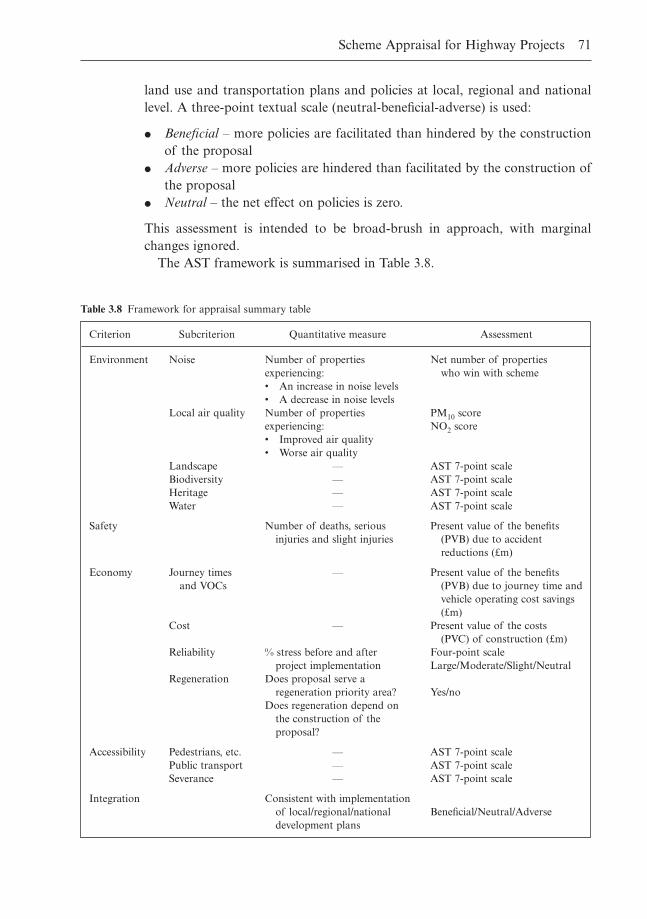
Scheme Appraisal for Highway Projects 71
land use and transportation plans and policies at local, regional and nationallevel. A three-point textual scale (neutral-beneficial-adverse) is used:
� Beneficial – more policies are facilitated than hindered by the constructionof the proposal
� Adverse – more policies are hindered than facilitated by the construction ofthe proposal
� Neutral – the net effect on policies is zero.
This assessment is intended to be broad-brush in approach, with marginalchanges ignored.
The AST framework is summarised in Table 3.8.
Criterion Subcriterion Quantitative measure Assessment
Environment Noise Number of properties Net number of propertiesexperiencing: who win with scheme• An increase in noise levels• A decrease in noise levels
Local air quality Number of properties PM10 scoreexperiencing: NO2 score• Improved air quality• Worse air quality
Landscape — AST 7-point scaleBiodiversity — AST 7-point scaleHeritage — AST 7-point scaleWater — AST 7-point scale
Safety Number of deaths, serious Present value of the benefitsinjuries and slight injuries (PVB) due to accident
reductions (£m)
Economy Journey times — Present value of the benefitsand VOCs (PVB) due to journey time and
vehicle operating cost savings(£m)
Cost — Present value of the costs(PVC) of construction (£m)
Reliability % stress before and after Four-point scaleproject implementation Large/Moderate/Slight/Neutral
Regeneration Does proposal serve aregeneration priority area? Yes/no
Does regeneration depend onthe construction of theproposal?
Accessibility Pedestrians, etc. — AST 7-point scalePublic transport — AST 7-point scaleSeverance — AST 7-point scale
Integration Consistent with implementationof local/regional/national Beneficial/Neutral/Adversedevelopment plans
Table 3.8 Framework for appraisal summary table
72 Highway Engineering
3.7 Summary
This chapter summarises the main types of methodologies for assessing thedesirability both in economic and in environmental/social terms of construct-ing a highway proposal. While the economic techniques may have been the firstto gain widespread acceptance, there is now a broad awareness, both within theUK and in Europe as a whole, as well as the US, that highway appraisal mustbe as inclusive a process as possible. Such concerns were the catalyst for theintroduction of the environmental impact assessment process. This inclusivenessrequires that the deliberations of as many as possible of the groupings affectedby the proposed scheme should be sought, and that the scheme’s viability shouldbe judged on as broad a range of objectives/criteria as possible.
3.8 References
Adler, H.A. (1987) Economic Appraisal of Transport Projects: A Manual with CaseStudies. EDI Series in Economic Development, Johns Hopkins University Press,London (Published for the World Bank).
Council of the European Communities (1985) On the assessment of the effects of certainpublic and private projects on the environment. Official Journal L175, 28.5.85, 40–48(85/337/EEC).
DoT (1982) Department of Transport COBA: A method of economic appraisal of highwayschemes. The Stationery Office, London.
DoT (1993) Department of Transport Design Manual for Roads and Bridges, Vol. 11:Environmental Impact Assessment. The Stationery Office, London.
Hill, M. (1973) Planning for Multiple Objectives: An Approach to the Evaluation of Trans-portation Plans. Technion, Philadelphia, USA.
Kelso, M.M. (1964) Economic analysis in the allocation of the federal budget to resourcedevelopment. In Economics and Public Policy in Water Resource Development (eds S.C.Smith & E.N. Castle) pp. 56–82. Iowa State University Press, USA.
Martin, J. C. (1993) The Successful Engineer: Personal and Professional Skills – A Source-book. McGraw-Hill International Editions, New York, USA.
Riggs, J.L., Bedworth, D.D. & Randhawa, S.U. (1997) Engineering Economics. McGraw-Hill International Editions, New York, USA.
Department of the Environment, Transport and the Regions DETR (1998) A Guidanceon the New Approach to Appraisal (NATA), September. The Stationery Office, London.
Zey, M. (1992) Criticisms of rational choice models. In Decision Making: Alternatives toRational Choice Models. Sage, Newbury Park, California, USA.
Chapter 4
Basic Elements of Highway Traffic Analysis
4.1 Introduction
The functional effectiveness of a highway is measured in terms of its ability toassist and accommodate the flow of vehicles with both safety and efficiency. Inorder to measure its level of effectiveness, certain parameters associated withthe highway must be measured and analysed. These properties include:
� The quantity of traffic� The type of vehicles within the traffic stream� The distribution of flow over a period of time (usually 24 hours)� The average speed of the traffic stream� The density of the traffic flow.
Analysis of these parameters will directly influence the scale and layout ofthe proposed highway, together with the type and quantity of materials used inits construction. This process of examination is termed traffic analysis and thesections below deal with relationships between the parameters which lie at itsbasis.
4.2 Speed, flow and density of a stream of traffic
The traffic flow, q, a measure of the volume of traffic on a highway, is definedas the number of vehicles, n, passing some given point on the highway in a giventime interval, t, i.e.:
(4.1)
In general terms, q is expressed in vehicles per unit time.The number of vehicles on a given section of highway can also be computed
in terms of the density or concentration of traffic as follows:
(4.2)knl
=
qnt
=
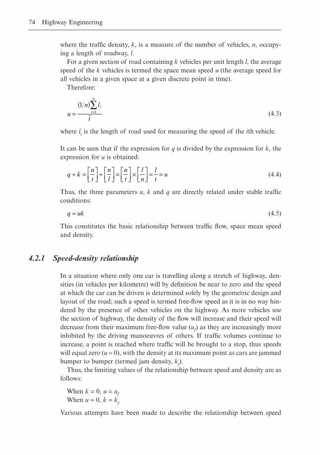
where the traffic density, k, is a measure of the number of vehicles, n, occupy-ing a length of roadway, l.
For a given section of road containing k vehicles per unit length l, the averagespeed of the k vehicles is termed the space mean speed u (the average speed forall vehicles in a given space at a given discrete point in time).
Therefore:
(4.3)
where li is the length of road used for measuring the speed of the ith vehicle.
It can be seen that if the expression for q is divided by the expression for k, theexpression for u is obtained:
(4.4)
Thus, the three parameters u, k and q are directly related under stable trafficconditions:
(4.5)
This constitutes the basic relationship between traffic flow, space mean speedand density.
4.2.1 Speed-density relationship
In a situation where only one car is travelling along a stretch of highway, den-sities (in vehicles per kilometre) will by definition be near to zero and the speedat which the car can be driven is determined solely by the geometric design andlayout of the road; such a speed is termed free-flow speed as it is in no way hin-dered by the presence of other vehicles on the highway. As more vehicles usethe section of highway, the density of the flow will increase and their speed willdecrease from their maximum free-flow value (uf) as they are increasingly moreinhibited by the driving manoeuvres of others. If traffic volumes continue toincrease, a point is reached where traffic will be brought to a stop, thus speedswill equal zero (u = 0), with the density at its maximum point as cars are jammedbumper to bumper (termed jam density, kj).
Thus, the limiting values of the relationship between speed and density are asfollows:
When k = 0, u = ufWhen u = 0, k = kj.
Various attempts have been made to describe the relationship between speed
q uk=
q knt
nl
nt
ln
lt
u∏ = ÈÎÍ
˘˚̇
∏ ÈÎÍ
˘˚̇
= ÈÎÍ
˘˚̇
¥ ÈÎÍ
˘˚̇
= =
un l
t
ii
n
=( )
=Â1
1
74 Highway Engineering
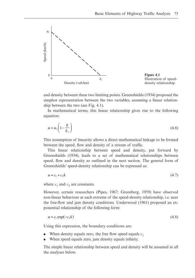
and density between these two limiting points. Greenshields (1934) proposed thesimplest representation between the two variables, assuming a linear relation-ship between the two (see Fig. 4.1).
In mathematical terms, this linear relationship gives rise to the following equation:
(4.6)
This assumption of linearity allows a direct mathematical linkage to be formedbetween the speed, flow and density of a stream of traffic.
This linear relationship between speed and density, put forward by Greenshields (1934), leads to a set of mathematical relationships between speed, flow and density as outlined in the next section. The general form ofGreenshields’ speed-density relationship can be expressed as:
(4.7)
where c1 and c2 are constants.
However, certain researchers (Pipes, 1967; Greenberg, 1959) have observed non-linear behaviour at each extreme of the speed-density relationship, i.e. nearthe free-flow and jam density conditions. Underwood (1961) proposed an ex-ponential relationship of the following form:
(4.8)
Using this expression, the boundary conditions are:
� When density equals zero, the free flow speed equals c1� When speed equals zero, jam density equals infinity.
The simple linear relationship between speed and density will be assumed in allthe analyses below.
u c c k= -( )1 2exp
u c c k= +1 2
u ukkf
j
= -ÊËÁ
ˆ¯̃1
Basic Elements of Highway Traffic Analysis 75
uf
kj 0
0
Spee
d (k
m/h
)
Density (veh/km)
Figure 4.1Illustration of speed-density relationship.
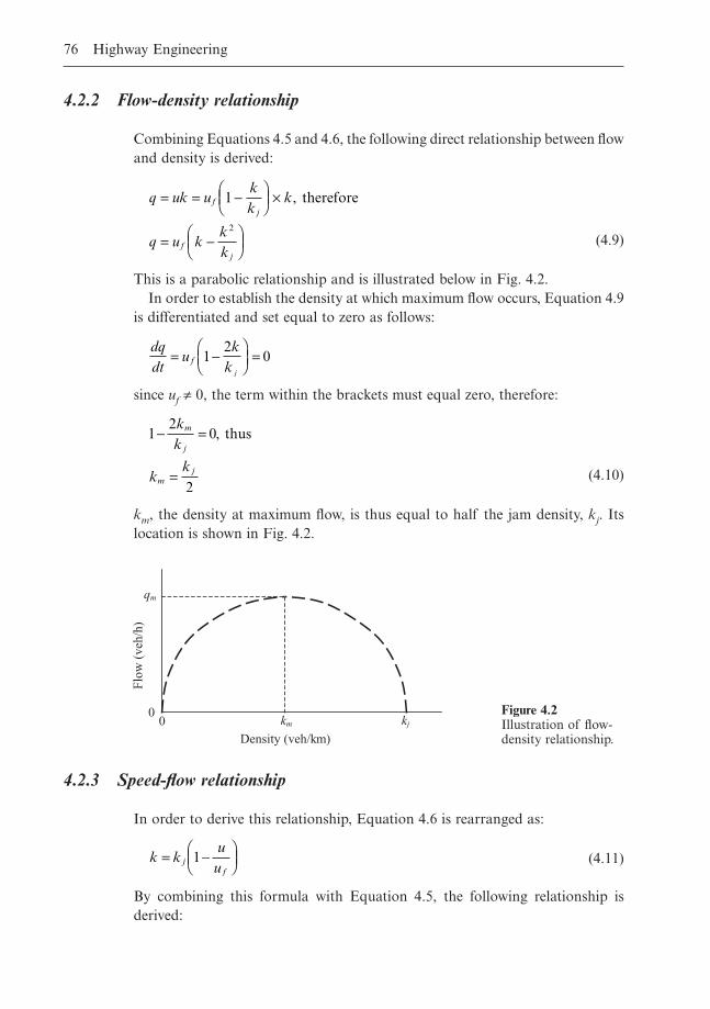
4.2.2 Flow-density relationship
Combining Equations 4.5 and 4.6, the following direct relationship between flowand density is derived:
(4.9)
This is a parabolic relationship and is illustrated below in Fig. 4.2.In order to establish the density at which maximum flow occurs, Equation 4.9
is differentiated and set equal to zero as follows:
since uf π 0, the term within the brackets must equal zero, therefore:
(4.10)
km, the density at maximum flow, is thus equal to half the jam density, kj. Itslocation is shown in Fig. 4.2.
12
0
2
- =
=
kk
kk
m
j
mj
, thus
dqdt
uk
kfj
= -ÊËÁ
ˆ¯̃
=12
0
q uk ukk
k
q u kkk
fj
fj
= = -ÊËÁ
ˆ¯̃
¥
= -ÊËÁ
ˆ¯̃
1
2
, therefore
76 Highway Engineering
00
qm
km kj
Density (veh/km)
Flow
(ve
h/h)
Figure 4.2Illustration of flow-density relationship.
4.2.3 Speed-flow relationship
In order to derive this relationship, Equation 4.6 is rearranged as:
(4.11)
By combining this formula with Equation 4.5, the following relationship isderived:
k ku
ujf
= -ÊËÁ
ˆ¯̃1
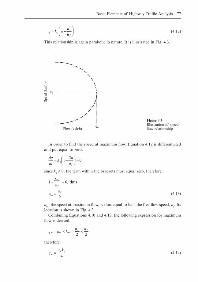
(4.12)
This relationship is again parabolic in nature. It is illustrated in Fig. 4.3.
q k uuuj
f
= -ÊËÁ
ˆ¯̃
2
Basic Elements of Highway Traffic Analysis 77
Flow (veh/h) qm
um
Spee
d (k
m/h
)
Figure 4.3Illustration of speed-flow relationship.
In order to find the speed at maximum flow, Equation 4.12 is differentiatedand put equal to zero:
since kj π 0, the term within the brackets must equal zero, therefore:
(4.13)
um, the speed at maximum flow, is thus equal to half the free-flow speed, uf. Itslocation is shown in Fig. 4.3.
Combining Equations 4.10 and 4.13, the following expression for maximumflow is derived:
therefore
(4.14) q
u km
f j=4
q u k
u km m m
f j= ¥ = ¥2 2
12
0
2
- =
=
uu
uu
m
f
mf
, thus
dqdt
ku
ujf
= -ÊËÁ
ˆ¯̃ =1
20
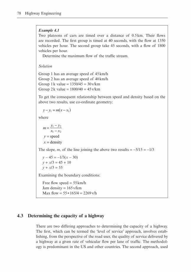
4.3 Determining the capacity of a highway
There are two differing approaches to determining the capacity of a highway.The first, which can be termed the ‘level of service’ approach, involves estab-lishing, from the perspective of the road user, the quality of service delivered bya highway at a given rate of vehicular flow per lane of traffic. The methodol-ogy is predominant in the US and other countries. The second approach, used
78 Highway Engineering
Example 4.1Two platoons of cars are timed over a distance of 0.5km. Their flows are recorded. The first group is timed at 40 seconds, with the flow at 1350vehicles per hour. The second group take 45 seconds, with a flow of 1800vehicles per hour.
Determine the maximum flow of the traffic stream.
Solution
Group 1 has an average speed of 45km/hGroup 2 has an average speed of 40km/hGroup 1k value = 1350/45 = 30v/kmGroup 2k value = 1800/40 = 45v/km
To get the consequent relationship between speed and density based on theabove two results, use co-ordinate geometry:
where
The slope, m, of the line joining the above two results = -5/15 = -1/3
y - 45 = -1/3(x - 30)y + x/3 = 45 + 10y + x/3 = 55
Examining the boundary conditions:
Free flow speed = 55km/hJam density = 165v/kmMax flow = 55*165/4 = 2269v/h
my yx x
y
x
=--
==
1 2
1 2
speed
density
y y m x x- = -( )1 1
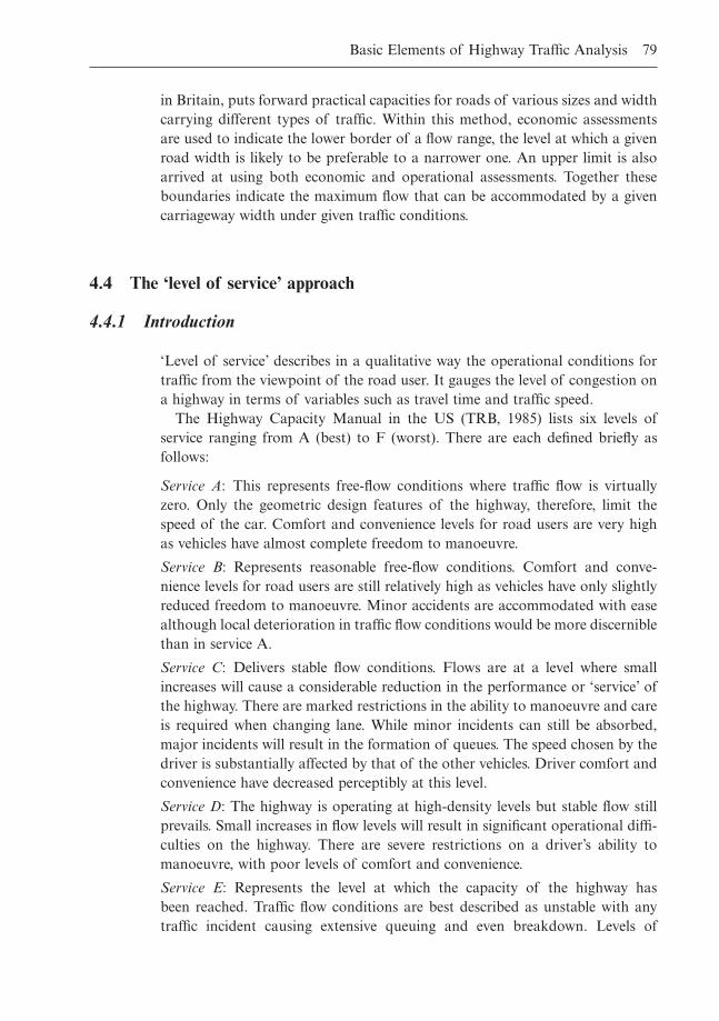
in Britain, puts forward practical capacities for roads of various sizes and widthcarrying different types of traffic. Within this method, economic assessmentsare used to indicate the lower border of a flow range, the level at which a givenroad width is likely to be preferable to a narrower one. An upper limit is alsoarrived at using both economic and operational assessments. Together theseboundaries indicate the maximum flow that can be accommodated by a givencarriageway width under given traffic conditions.
4.4 The ‘level of service’ approach
4.4.1 Introduction
‘Level of service’ describes in a qualitative way the operational conditions fortraffic from the viewpoint of the road user. It gauges the level of congestion ona highway in terms of variables such as travel time and traffic speed.
The Highway Capacity Manual in the US (TRB, 1985) lists six levels ofservice ranging from A (best) to F (worst). There are each defined briefly asfollows:
Service A: This represents free-flow conditions where traffic flow is virtuallyzero. Only the geometric design features of the highway, therefore, limit thespeed of the car. Comfort and convenience levels for road users are very highas vehicles have almost complete freedom to manoeuvre.
Service B: Represents reasonable free-flow conditions. Comfort and conve-nience levels for road users are still relatively high as vehicles have only slightlyreduced freedom to manoeuvre. Minor accidents are accommodated with easealthough local deterioration in traffic flow conditions would be more discerniblethan in service A.
Service C: Delivers stable flow conditions. Flows are at a level where smallincreases will cause a considerable reduction in the performance or ‘service’ ofthe highway. There are marked restrictions in the ability to manoeuvre and careis required when changing lane. While minor incidents can still be absorbed,major incidents will result in the formation of queues. The speed chosen by thedriver is substantially affected by that of the other vehicles. Driver comfort andconvenience have decreased perceptibly at this level.
Service D: The highway is operating at high-density levels but stable flow stillprevails. Small increases in flow levels will result in significant operational diffi-culties on the highway. There are severe restrictions on a driver’s ability tomanoeuvre, with poor levels of comfort and convenience.
Service E: Represents the level at which the capacity of the highway has been reached. Traffic flow conditions are best described as unstable with anytraffic incident causing extensive queuing and even breakdown. Levels of
Basic Elements of Highway Traffic Analysis 79
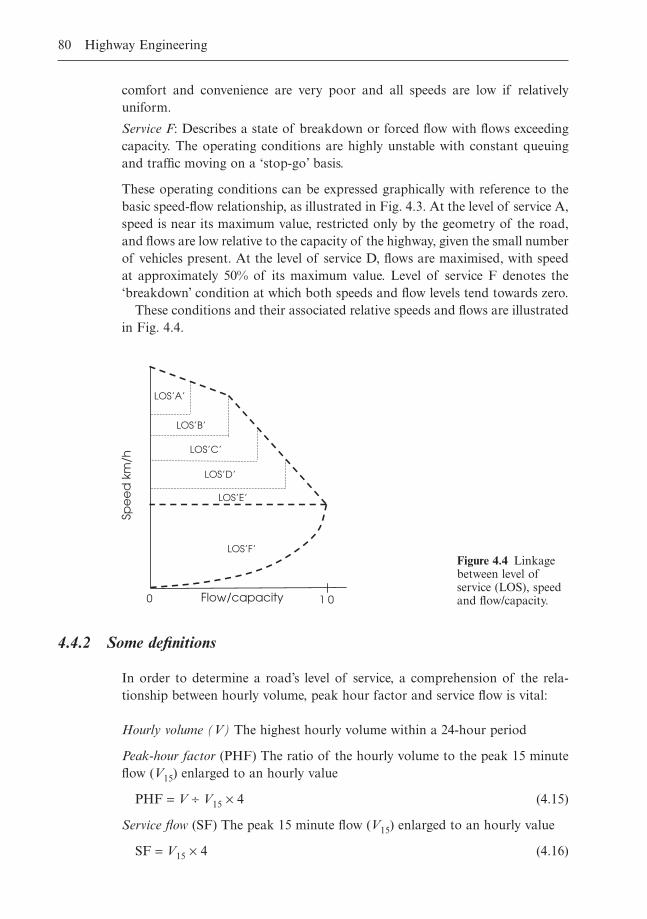
comfort and convenience are very poor and all speeds are low if relativelyuniform.
Service F: Describes a state of breakdown or forced flow with flows exceedingcapacity. The operating conditions are highly unstable with constant queuingand traffic moving on a ‘stop-go’ basis.
These operating conditions can be expressed graphically with reference to thebasic speed-flow relationship, as illustrated in Fig. 4.3. At the level of service A,speed is near its maximum value, restricted only by the geometry of the road,and flows are low relative to the capacity of the highway, given the small numberof vehicles present. At the level of service D, flows are maximised, with speedat approximately 50% of its maximum value. Level of service F denotes the‘breakdown’ condition at which both speeds and flow levels tend towards zero.
These conditions and their associated relative speeds and flows are illustratedin Fig. 4.4.
80 Highway Engineering
0
LOS’A’
LOS’B’
LOS’C’
LOS’D’
LOS’E’
LOS’F’
Flow/capacity
Spe
ed
km
/h
1 0
Figure 4.4 Linkagebetween level ofservice (LOS), speedand flow/capacity.
4.4.2 Some definitions
In order to determine a road’s level of service, a comprehension of the rela-tionship between hourly volume, peak hour factor and service flow is vital:
Hourly volume (V) The highest hourly volume within a 24-hour period
Peak-hour factor (PHF) The ratio of the hourly volume to the peak 15 minuteflow (V15) enlarged to an hourly value
PHF = V ∏ V15 ¥ 4 (4.15)
Service flow (SF) The peak 15 minute flow (V15) enlarged to an hourly value
SF = V15 ¥ 4 (4.16)
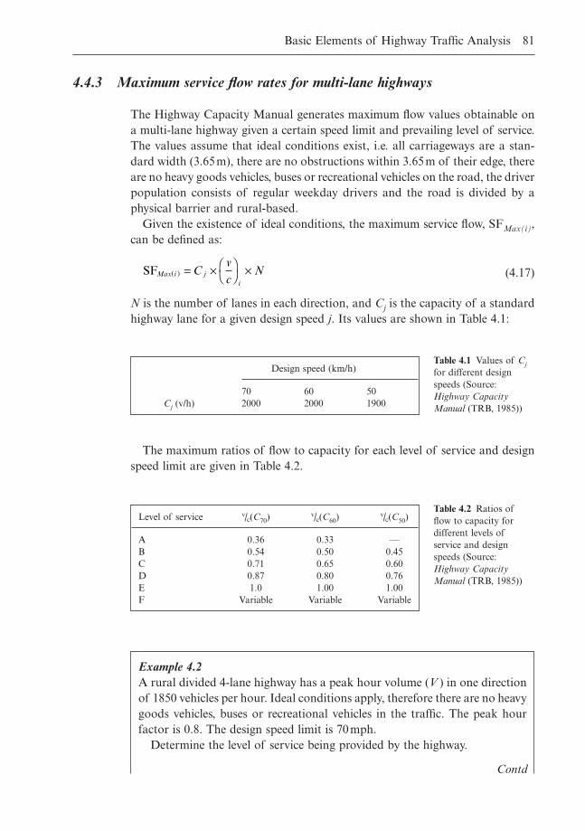
4.4.3 Maximum service flow rates for multi-lane highways
The Highway Capacity Manual generates maximum flow values obtainable ona multi-lane highway given a certain speed limit and prevailing level of service.The values assume that ideal conditions exist, i.e. all carriageways are a stan-dard width (3.65m), there are no obstructions within 3.65m of their edge, thereare no heavy goods vehicles, buses or recreational vehicles on the road, the driverpopulation consists of regular weekday drivers and the road is divided by a physical barrier and rural-based.
Given the existence of ideal conditions, the maximum service flow, SFMax(i),can be defined as:
(4.17)
N is the number of lanes in each direction, and Cj is the capacity of a standardhighway lane for a given design speed j. Its values are shown in Table 4.1:
SFMax i ji
Cvc
N( ) = ¥ ÊË
ˆ¯ ¥
Basic Elements of Highway Traffic Analysis 81
Design speed (km/h)
70 60 50Cj (v/h) 2000 2000 1900
Table 4.1 Values of Cjfor different designspeeds (Source:Highway CapacityManual (TRB, 1985))
Level of service v/c(C70)v/c(C60)
v/c(C50)
A 0.36 0.33 —B 0.54 0.50 0.45C 0.71 0.65 0.60D 0.87 0.80 0.76E 1.0 1.00 1.00F Variable Variable Variable
Table 4.2 Ratios offlow to capacity fordifferent levels ofservice and designspeeds (Source:Highway CapacityManual (TRB, 1985))
The maximum ratios of flow to capacity for each level of service and designspeed limit are given in Table 4.2.
Example 4.2A rural divided 4-lane highway has a peak hour volume (V ) in one directionof 1850 vehicles per hour. Ideal conditions apply, therefore there are no heavygoods vehicles, buses or recreational vehicles in the traffic. The peak hourfactor is 0.8. The design speed limit is 70mph.
Determine the level of service being provided by the highway.
Contd
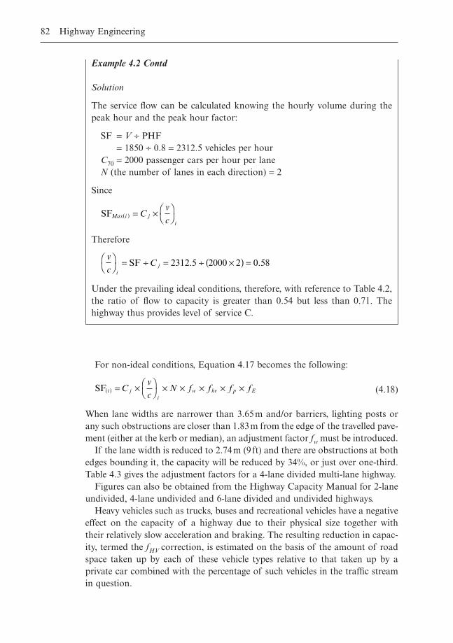
For non-ideal conditions, Equation 4.17 becomes the following:
(4.18)
When lane widths are narrower than 3.65m and/or barriers, lighting posts orany such obstructions are closer than 1.83m from the edge of the travelled pave-ment (either at the kerb or median), an adjustment factor fw must be introduced.
If the lane width is reduced to 2.74m (9 ft) and there are obstructions at bothedges bounding it, the capacity will be reduced by 34%, or just over one-third.Table 4.3 gives the adjustment factors for a 4-lane divided multi-lane highway.
Figures can also be obtained from the Highway Capacity Manual for 2-laneundivided, 4-lane undivided and 6-lane divided and undivided highways.
Heavy vehicles such as trucks, buses and recreational vehicles have a negativeeffect on the capacity of a highway due to their physical size together with their relatively slow acceleration and braking. The resulting reduction in capac-ity, termed the fHV correction, is estimated on the basis of the amount of roadspace taken up by each of these vehicle types relative to that taken up by aprivate car combined with the percentage of such vehicles in the traffic streamin question.
SF i ji
w hv p ECvc
N f f f f( ) = ¥ ÊË
ˆ¯ ¥ ¥ ¥ ¥ ¥
82 Highway Engineering
Example 4.2 Contd
Solution
The service flow can be calculated knowing the hourly volume during thepeak hour and the peak hour factor:
SF = V ∏ PHF= 1850 ∏ 0.8 = 2312.5 vehicles per hour
C70 = 2000 passenger cars per hour per laneN (the number of lanes in each direction) = 2
Since
Therefore
Under the prevailing ideal conditions, therefore, with reference to Table 4.2,the ratio of flow to capacity is greater than 0.54 but less than 0.71. Thehighway thus provides level of service C.
vc
Ci
jÊË
ˆ¯ = ∏ = ∏ ¥( ) =SF 2312 5 2000 2 0 58. .
SFMax i ji
Cvc
( ) = ¥ ÊË
ˆ¯
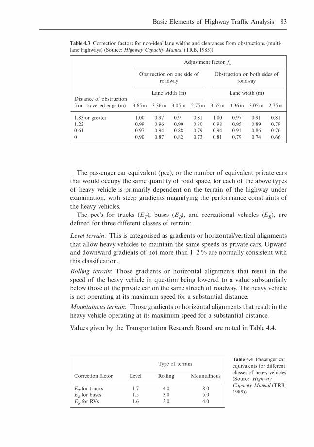
The passenger car equivalent (pce), or the number of equivalent private carsthat would occupy the same quantity of road space, for each of the above typesof heavy vehicle is primarily dependent on the terrain of the highway underexamination, with steep gradients magnifying the performance constraints ofthe heavy vehicles.
The pce’s for trucks (ET), buses (EB), and recreational vehicles (ER), aredefined for three different classes of terrain:
Level terrain: This is categorised as gradients or horizontal/vertical alignmentsthat allow heavy vehicles to maintain the same speeds as private cars. Upwardand downward gradients of not more than 1–2 % are normally consistent withthis classification.
Rolling terrain: Those gradients or horizontal alignments that result in thespeed of the heavy vehicle in question being lowered to a value substantiallybelow those of the private car on the same stretch of roadway. The heavy vehicleis not operating at its maximum speed for a substantial distance.
Mountainous terrain: Those gradients or horizontal alignments that result in theheavy vehicle operating at its maximum speed for a substantial distance.
Values given by the Transportation Research Board are noted in Table 4.4.
Basic Elements of Highway Traffic Analysis 83
Adjustment factor, fw
Obstruction on one side of Obstruction on both sides ofroadway roadway
Distance of obstructionLane width (m) Lane width (m)
from travelled edge (m) 3.65m 3.36m 3.05m 2.75m 3.65m 3.36m 3.05m 2.75m
1.83 or greater 1.00 0.97 0.91 0.81 1.00 0.97 0.91 0.811.22 0.99 0.96 0.90 0.80 0.98 0.95 0.89 0.790.61 0.97 0.94 0.88 0.79 0.94 0.91 0.86 0.760 0.90 0.87 0.82 0.73 0.81 0.79 0.74 0.66
Table 4.3 Correction factors for non-ideal lane widths and clearances from obstructions (multi-lane highways) (Source: Highway Capacity Manual (TRB, 1985))
Type of terrain
Correction factor Level Rolling Mountainous
ET for trucks 1.7 4.0 8.0EB for buses 1.5 3.0 5.0ER for RVs 1.6 3.0 4.0
Table 4.4 Passenger carequivalents for differentclasses of heavy vehicles(Source: HighwayCapacity Manual (TRB,1985))
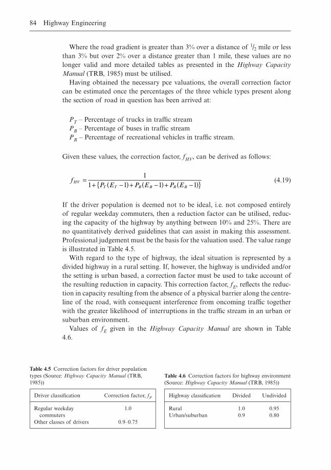
Where the road gradient is greater than 3% over a distance of 1/2 mile or lessthan 3% but over 2% over a distance greater than 1 mile, these values are nolonger valid and more detailed tables as presented in the Highway CapacityManual (TRB, 1985) must be utilised.
Having obtained the necessary pce valuations, the overall correction factorcan be estimated once the percentages of the three vehicle types present alongthe section of road in question has been arrived at:
PT – Percentage of trucks in traffic streamPB – Percentage of buses in traffic streamPR – Percentage of recreational vehicles in traffic stream.
Given these values, the correction factor, fHV, can be derived as follows:
(4.19)
If the driver population is deemed not to be ideal, i.e. not composed entirely of regular weekday commuters, then a reduction factor can be utilised, reduc-ing the capacity of the highway by anything between 10% and 25%. There areno quantitatively derived guidelines that can assist in making this assessment.Professional judgement must be the basis for the valuation used. The value rangeis illustrated in Table 4.5.
With regard to the type of highway, the ideal situation is represented by adivided highway in a rural setting. If, however, the highway is undivided and/orthe setting is urban based, a correction factor must be used to take account ofthe resulting reduction in capacity. This correction factor, fE, reflects the reduc-tion in capacity resulting from the absence of a physical barrier along the centre-line of the road, with consequent interference from oncoming traffic togetherwith the greater likelihood of interruptions in the traffic stream in an urban orsuburban environment.
Values of fE given in the Highway Capacity Manual are shown in Table 4.6.
fP E P E P EHV
T T B B R R
=+ -( ) + -( ) + -( ){ }
11 1 1 1
84 Highway Engineering
Driver classification Correction factor, fP
Regular weekday 1.0commuters
Other classes of drivers 0.9–0.75
Table 4.5 Correction factors for driver populationtypes (Source: Highway Capacity Manual (TRB,1985))
Highway classification Divided Undivided
Rural 1.0 0.95Urban/suburban 0.9 0.80
Table 4.6 Correction factors for highway environment(Source: Highway Capacity Manual (TRB, 1985))
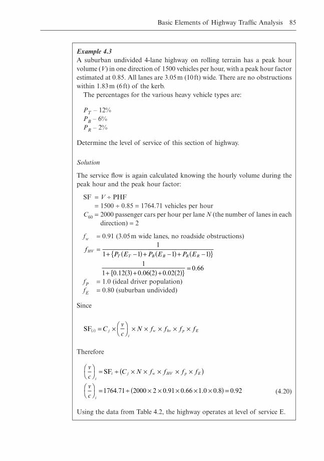
Basic Elements of Highway Traffic Analysis 85
Example 4.3A suburban undivided 4-lane highway on rolling terrain has a peak hourvolume (V) in one direction of 1500 vehicles per hour, with a peak hour factorestimated at 0.85. All lanes are 3.05m (10 ft) wide. There are no obstructionswithin 1.83m (6 ft) of the kerb.
The percentages for the various heavy vehicle types are:
PT – 12%PB – 6%PR – 2%
Determine the level of service of this section of highway.
Solution
The service flow is again calculated knowing the hourly volume during thepeak hour and the peak hour factor:
SF = V ∏ PHF= 1500 ∏ 0.85 = 1764.71 vehicles per hour
C60 = 2000 passenger cars per hour per lane N (the number of lanes in eachdirection) = 2
fw = 0.91 (3.05m wide lanes, no roadside obstructions)
fP = 1.0 (ideal driver population)fE = 0.80 (suburban undivided)
Since
Therefore
(4.20)
Using the data from Table 4.2, the highway operates at level of service E.
vc
C N f f f f
vc
ii j w HV p E
i
ÊË
ˆ¯ = ∏ ¥ ¥ ¥ ¥ ¥( )
ÊË
ˆ¯ = ∏ ¥ ¥ ¥ ¥ ¥( ) =
SF
1764 71 2000 2 0 91 0 66 1 0 0 8 0 92. . . . . .
SF i ji
w hv p ECvc
N f f f f( ) = ¥ ÊË
ˆ¯ ¥ ¥ ¥ ¥ ¥
fP E P E P EHV
T T B B R R
=+ -( ) + -( ) + -( ){ }
+ ( ) + ( ) + ( ){ } =
11 1 1 1
11 0 12 3 0 06 2 0 02 2
0 66. . .
.
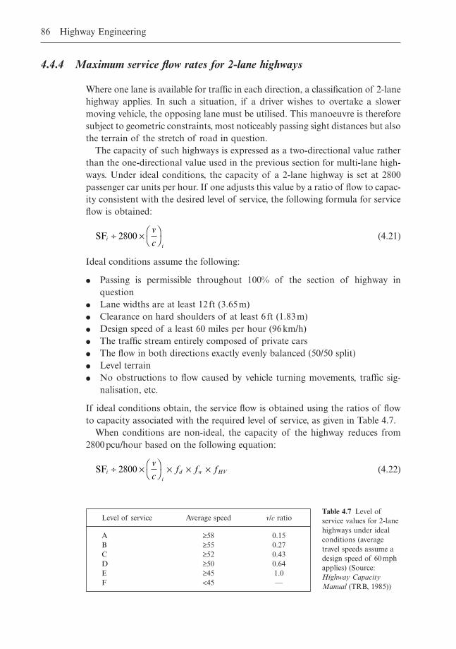
4.4.4 Maximum service flow rates for 2-lane highways
Where one lane is available for traffic in each direction, a classification of 2-lanehighway applies. In such a situation, if a driver wishes to overtake a slowermoving vehicle, the opposing lane must be utilised. This manoeuvre is thereforesubject to geometric constraints, most noticeably passing sight distances but alsothe terrain of the stretch of road in question.
The capacity of such highways is expressed as a two-directional value ratherthan the one-directional value used in the previous section for multi-lane high-ways. Under ideal conditions, the capacity of a 2-lane highway is set at 2800passenger car units per hour. If one adjusts this value by a ratio of flow to capac-ity consistent with the desired level of service, the following formula for serviceflow is obtained:
(4.21)
Ideal conditions assume the following:
� Passing is permissible throughout 100% of the section of highway in question
� Lane widths are at least 12 ft (3.65m)� Clearance on hard shoulders of at least 6 ft (1.83m)� Design speed of a least 60 miles per hour (96km/h)� The traffic stream entirely composed of private cars� The flow in both directions exactly evenly balanced (50/50 split)� Level terrain� No obstructions to flow caused by vehicle turning movements, traffic sig-
nalisation, etc.
If ideal conditions obtain, the service flow is obtained using the ratios of flowto capacity associated with the required level of service, as given in Table 4.7.
When conditions are non-ideal, the capacity of the highway reduces from2800pcu/hour based on the following equation:
(4.22)SFii
d w HVvc
f f f∏ ¥ ÊË
ˆ¯ ¥ ¥ ¥2800
SFii
vc
∏ ¥ ÊË
ˆ¯2800
86 Highway Engineering
Level of service Average speed v/c ratio
A ≥58 0.15B ≥55 0.27C ≥52 0.43D ≥50 0.64E ≥45 1.0F <45 —
Table 4.7 Level ofservice values for 2-lanehighways under idealconditions (averagetravel speeds assume adesign speed of 60mphapplies) (Source:Highway CapacityManual (TRB, 1985))
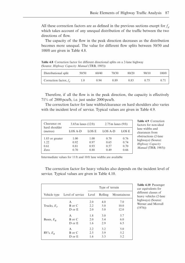
All these correction factors are as defined in the previous sections except for fdwhich takes account of any unequal distribution of the traffic between the twodirections of flow.
The capacity of the flow in the peak direction decreases as the distributionbecomes more unequal. The value for different flow splits between 50/50 and100/0 are given in Table 4.8.
Basic Elements of Highway Traffic Analysis 87
Distributional split 50/50 60/40 70/30 80/20 90/10 100/0
Correction factor, fd 1.0 0.94 0.89 0.83 0.75 0.71
Table 4.8 Correction factor for different directional splits on a 2-lane highway (Source: Highway Capacity Manual (TRB, 1985))
Therefore, if all the flow is in the peak direction, the capacity is effectively71% of 2800pcu/h, i.e. just under 2000pcu/h.
The correction factor for lane widths/clearance on hard shoulders also varieswith the incident level of service. Typical values are given in Table 4.9.
Clearance onhard shoulder
3.65m lanes (12 ft) 2.75m lanes (9 ft)
(metres) LOS A-D LOS E LOS A-D LOS E
1.83 or greater 1.00 1.00 0.70 0.761.22 0.92 0.97 0.65 0.740.61 0.81 0.93 0.57 0.70Zero 0.70 0.88 0.49 0.66
Table 4.9 Correctionfactors for non-ideallane widths andclearances fromobstructions (2-lanehighways) (Source:Highway CapacityManual (TRB, 1985))
Intermediate values for 11 ft and 10 ft lane widths are available
The correction factor for heavy vehicles also depends on the incident level ofservice. Typical values are given in Table 4.10.
Type of terrain
Vehicle type Level of service Level Rolling Mountainous
A 2.0 4.0 7.0Trucks, ET B or C 2.2 5.0 10.0
D or E 2.0 5.0 12.0
A 1.8 3.0 5.7Buses, EB B or C 2.0 3.4 6.0
D or E 1.6 2.9 6.5
A 2.2 3.2 5.0RV’s, ER B or C 2.5 3.9 5.2
D or E 1.6 3.3 5.2
Table 4.10 Passengercar equivalents fordifferent classes ofheavy vehicles (2-lanehighways) (Source:Werner and Morrall(1976))
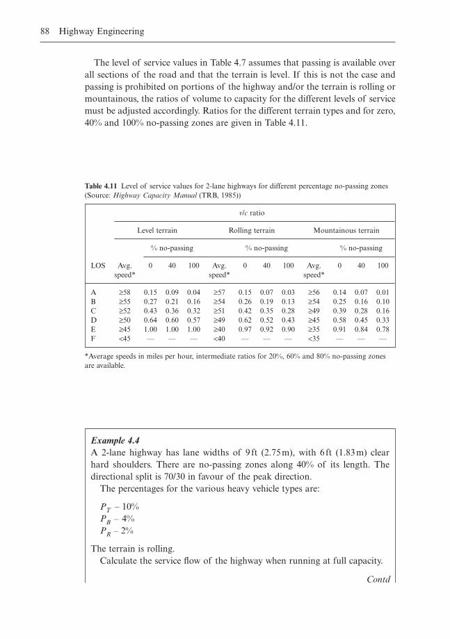
Example 4.4A 2-lane highway has lane widths of 9 ft (2.75m), with 6 ft (1.83m) clear hard shoulders. There are no-passing zones along 40% of its length. Thedirectional split is 70/30 in favour of the peak direction.
The percentages for the various heavy vehicle types are:
PT – 10%PB – 4%PR – 2%
The terrain is rolling.Calculate the service flow of the highway when running at full capacity.
The level of service values in Table 4.7 assumes that passing is available overall sections of the road and that the terrain is level. If this is not the case andpassing is prohibited on portions of the highway and/or the terrain is rolling ormountainous, the ratios of volume to capacity for the different levels of servicemust be adjusted accordingly. Ratios for the different terrain types and for zero,40% and 100% no-passing zones are given in Table 4.11.
88 Highway Engineering
v/c ratio
Level terrain Rolling terrain Mountainous terrain
% no-passing % no-passing % no-passing
LOS Avg. 0 40 100 Avg. 0 40 100 Avg. 0 40 100speed* speed* speed*
A ≥58 0.15 0.09 0.04 ≥57 0.15 0.07 0.03 ≥56 0.14 0.07 0.01B ≥55 0.27 0.21 0.16 ≥54 0.26 0.19 0.13 ≥54 0.25 0.16 0.10C ≥52 0.43 0.36 0.32 ≥51 0.42 0.35 0.28 ≥49 0.39 0.28 0.16D ≥50 0.64 0.60 0.57 ≥49 0.62 0.52 0.43 ≥45 0.58 0.45 0.33E ≥45 1.00 1.00 1.00 ≥40 0.97 0.92 0.90 ≥35 0.91 0.84 0.78F <45 — — — <40 — — — <35 — — —
Table 4.11 Level of service values for 2-lane highways for different percentage no-passing zones(Source: Highway Capacity Manual (TRB, 1985))
*Average speeds in miles per hour, intermediate ratios for 20%, 60% and 80% no-passing zonesare available.
Contd
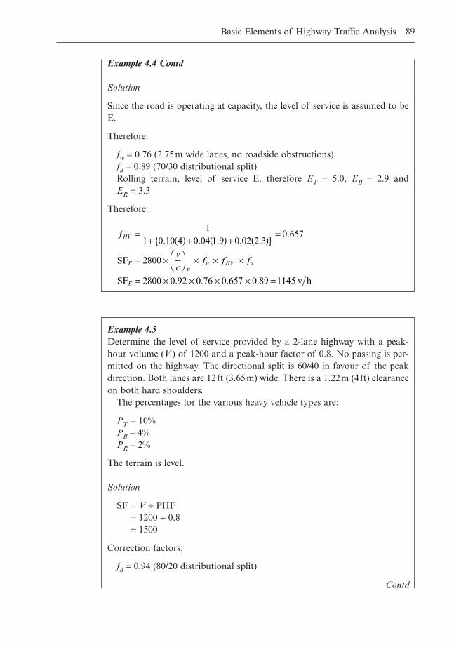
Basic Elements of Highway Traffic Analysis 89
Example 4.4 Contd
Solution
Since the road is operating at capacity, the level of service is assumed to beE.
Therefore:
fw = 0.76 (2.75m wide lanes, no roadside obstructions)fd = 0.89 (70/30 distributional split)Rolling terrain, level of service E, therefore ET = 5.0, EB = 2.9 and ER = 3.3
Therefore:
f
vc
f f f
HV
EE
w HV d
E
=+ ( ) + ( ) + ( ){ } =
= ¥ ÊË
ˆ¯ ¥ ¥ ¥
= ¥ ¥ ¥ ¥ =
11 0 10 4 0 04 1 9 0 02 2 3
0 657
2800
2800 0 92 0 76 0 657 0 89 1145
. . . . ..
. . . .
SF
SF v h
Example 4.5Determine the level of service provided by a 2-lane highway with a peak-hour volume (V ) of 1200 and a peak-hour factor of 0.8. No passing is per-mitted on the highway. The directional split is 60/40 in favour of the peakdirection. Both lanes are 12 ft (3.65m) wide. There is a 1.22m (4 ft) clearanceon both hard shoulders.
The percentages for the various heavy vehicle types are:
PT – 10%PB – 4%PR – 2%
The terrain is level.
Solution
SF = V ∏ PHF= 1200 ∏ 0.8= 1500
Correction factors:
fd = 0.94 (80/20 distributional split)
Contd
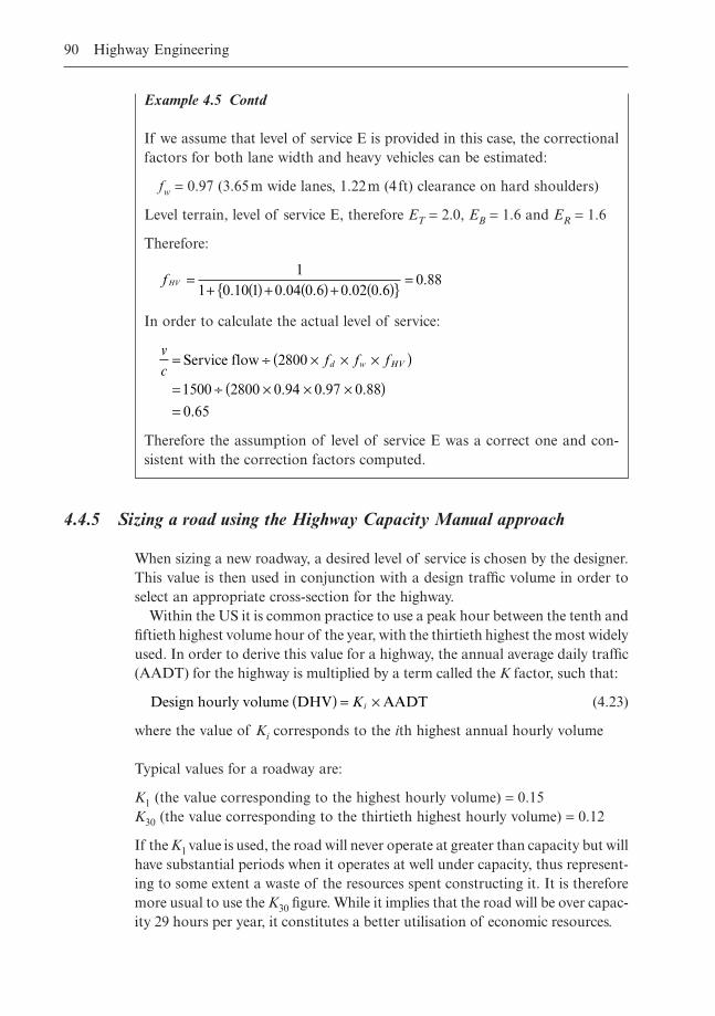
4.4.5 Sizing a road using the Highway Capacity Manual approach
When sizing a new roadway, a desired level of service is chosen by the designer.This value is then used in conjunction with a design traffic volume in order toselect an appropriate cross-section for the highway.
Within the US it is common practice to use a peak hour between the tenth andfiftieth highest volume hour of the year, with the thirtieth highest the most widelyused. In order to derive this value for a highway, the annual average daily traffic(AADT) for the highway is multiplied by a term called the K factor, such that:
(4.23)
where the value of Ki corresponds to the ith highest annual hourly volume
Typical values for a roadway are:
K1 (the value corresponding to the highest hourly volume) = 0.15K30 (the value corresponding to the thirtieth highest hourly volume) = 0.12
If the K1 value is used, the road will never operate at greater than capacity but willhave substantial periods when it operates at well under capacity, thus represent-ing to some extent a waste of the resources spent constructing it. It is thereforemore usual to use the K30 figure. While it implies that the road will be over capac-ity 29 hours per year, it constitutes a better utilisation of economic resources.
Design hourly volume DHV AADT( ) = ¥Ki
90 Highway Engineering
Example 4.5 Contd
If we assume that level of service E is provided in this case, the correctionalfactors for both lane width and heavy vehicles can be estimated:
fw = 0.97 (3.65m wide lanes, 1.22m (4 ft) clearance on hard shoulders)
Level terrain, level of service E, therefore ET = 2.0, EB = 1.6 and ER = 1.6
Therefore:
In order to calculate the actual level of service:
Therefore the assumption of level of service E was a correct one and con-sistent with the correction factors computed.
vc
f f fd w HV= ∏ ¥ ¥ ¥( )
= ∏ ¥ ¥ ¥( )=
Service flow 2800
1500 2800 0 94 0 97 0 88
0 65
. . .
.
fHV =+ ( ) + ( ) + ( ){ } =
11 0 10 1 0 04 0 6 0 02 0 6
0 88. . . . .
.
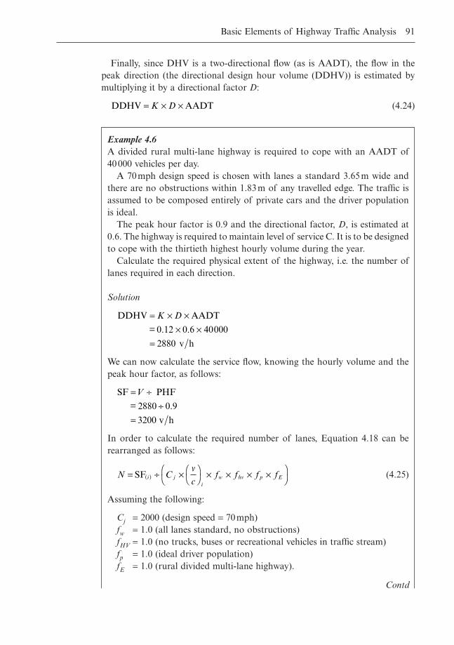
Finally, since DHV is a two-directional flow (as is AADT), the flow in thepeak direction (the directional design hour volume (DDHV)) is estimated bymultiplying it by a directional factor D:
(4.24)DDHV AADT= ¥ ¥K D
Basic Elements of Highway Traffic Analysis 91
Example 4.6A divided rural multi-lane highway is required to cope with an AADT of40000 vehicles per day.
A 70mph design speed is chosen with lanes a standard 3.65m wide andthere are no obstructions within 1.83m of any travelled edge. The traffic isassumed to be composed entirely of private cars and the driver populationis ideal.
The peak hour factor is 0.9 and the directional factor, D, is estimated at0.6. The highway is required to maintain level of service C. It is to be designedto cope with the thirtieth highest hourly volume during the year.
Calculate the required physical extent of the highway, i.e. the number oflanes required in each direction.
Solution
We can now calculate the service flow, knowing the hourly volume and thepeak hour factor, as follows:
In order to calculate the required number of lanes, Equation 4.18 can berearranged as follows:
(4.25)
Assuming the following:
Cj = 2000 (design speed = 70mph)fw = 1.0 (all lanes standard, no obstructions)fHV = 1.0 (no trucks, buses or recreational vehicles in traffic stream)fp = 1.0 (ideal driver population)fE = 1.0 (rural divided multi-lane highway).
N Cvc
f f f fi ji
w hv p E= ∏ ¥ ÊË
ˆ¯ ¥ ¥ ¥ ¥Ê
ˈ¯( )SF
SF PHF
= 2880
v h
= ∏∏
=
V
0 9
3200
.
DDHV AADT
= 0.12
v h
= ¥ ¥¥ ¥
=
K D
0 6 40000
2880
.
Contd
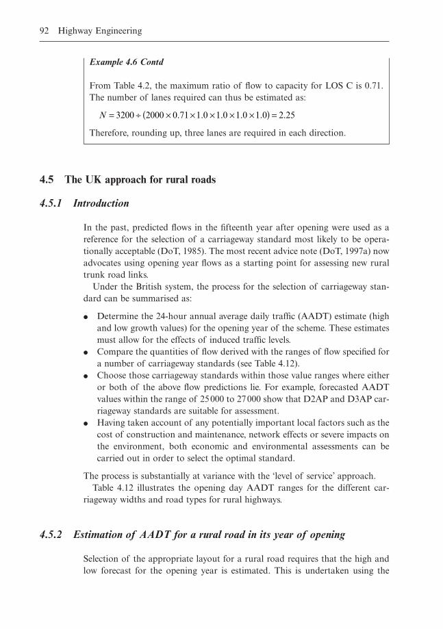
4.5 The UK approach for rural roads
4.5.1 Introduction
In the past, predicted flows in the fifteenth year after opening were used as areference for the selection of a carriageway standard most likely to be opera-tionally acceptable (DoT, 1985). The most recent advice note (DoT, 1997a) nowadvocates using opening year flows as a starting point for assessing new ruraltrunk road links.
Under the British system, the process for the selection of carriageway stan-dard can be summarised as:
� Determine the 24-hour annual average daily traffic (AADT) estimate (highand low growth values) for the opening year of the scheme. These estimatesmust allow for the effects of induced traffic levels.
� Compare the quantities of flow derived with the ranges of flow specified fora number of carriageway standards (see Table 4.12).
� Choose those carriageway standards within those value ranges where eitheror both of the above flow predictions lie. For example, forecasted AADTvalues within the range of 25000 to 27000 show that D2AP and D3AP car-riageway standards are suitable for assessment.
� Having taken account of any potentially important local factors such as thecost of construction and maintenance, network effects or severe impacts onthe environment, both economic and environmental assessments can becarried out in order to select the optimal standard.
The process is substantially at variance with the ‘level of service’ approach.Table 4.12 illustrates the opening day AADT ranges for the different car-
riageway widths and road types for rural highways.
4.5.2 Estimation of AADT for a rural road in its year of opening
Selection of the appropriate layout for a rural road requires that the high andlow forecast for the opening year is estimated. This is undertaken using the
92 Highway Engineering
Example 4.6 Contd
From Table 4.2, the maximum ratio of flow to capacity for LOS C is 0.71.The number of lanes required can thus be estimated as:
Therefore, rounding up, three lanes are required in each direction.
N = ∏ ¥ ¥ ¥ ¥ ¥( ) =3200 2000 0 71 1 0 1 0 1 0 1 0 2 25. . . . . .
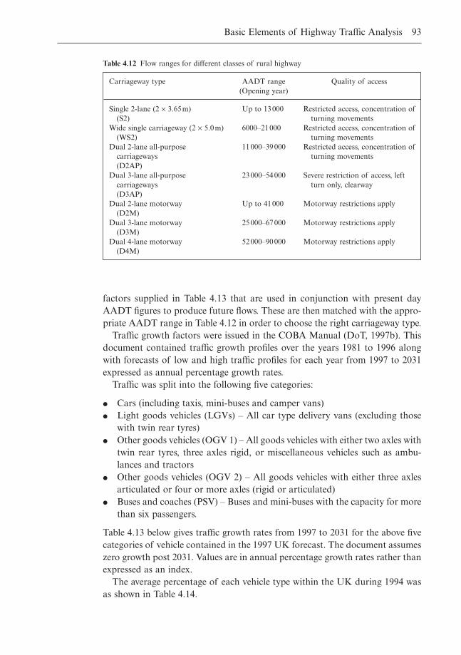
factors supplied in Table 4.13 that are used in conjunction with present dayAADT figures to produce future flows. These are then matched with the appro-priate AADT range in Table 4.12 in order to choose the right carriageway type.
Traffic growth factors were issued in the COBA Manual (DoT, 1997b). Thisdocument contained traffic growth profiles over the years 1981 to 1996 alongwith forecasts of low and high traffic profiles for each year from 1997 to 2031expressed as annual percentage growth rates.
Traffic was split into the following five categories:
� Cars (including taxis, mini-buses and camper vans)� Light goods vehicles (LGVs) – All car type delivery vans (excluding those
with twin rear tyres)� Other goods vehicles (OGV 1) – All goods vehicles with either two axles with
twin rear tyres, three axles rigid, or miscellaneous vehicles such as ambu-lances and tractors
� Other goods vehicles (OGV 2) – All goods vehicles with either three axlesarticulated or four or more axles (rigid or articulated)
� Buses and coaches (PSV) – Buses and mini-buses with the capacity for morethan six passengers.
Table 4.13 below gives traffic growth rates from 1997 to 2031 for the above fivecategories of vehicle contained in the 1997 UK forecast. The document assumeszero growth post 2031. Values are in annual percentage growth rates rather thanexpressed as an index.
The average percentage of each vehicle type within the UK during 1994 wasas shown in Table 4.14.
Basic Elements of Highway Traffic Analysis 93
Carriageway type AADT range Quality of access(Opening year)
Single 2-lane (2 ¥ 3.65m) Up to 13000 Restricted access, concentration of(S2) turning movements
Wide single carriageway (2 ¥ 5.0m) 6000–21000 Restricted access, concentration of(WS2) turning movements
Dual 2-lane all-purpose 11000–39000 Restricted access, concentration ofcarriageways turning movements(D2AP)
Dual 3-lane all-purpose 23000–54000 Severe restriction of access, leftcarriageways turn only, clearway(D3AP)
Dual 2-lane motorway Up to 41000 Motorway restrictions apply(D2M)
Dual 3-lane motorway 25000–67000 Motorway restrictions apply(D3M)
Dual 4-lane motorway 52000–90000 Motorway restrictions apply(D4M)
Table 4.12 Flow ranges for different classes of rural highway
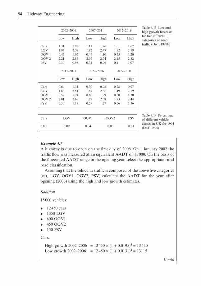
94 Highway Engineering
2002–2006 2007–2011 2012–2016
Low High Low High Low High
Cars 1.31 1.95 1.11 1.76 1.01 1.67LGV 1.93 2.58 1.82 2.48 1.92 2.59OGV 1 0.43 1.07 0.46 1.10 0.55 1.20OGV 2 2.21 2.85 2.09 2.74 2.15 2.82PSV 0.34 0.98 0.34 0.99 0.41 1.07
2017–2021 2022–2026 2027–2031
Low High Low High Low High
Cars 0.64 1.31 0.30 0.98 0.28 0.97LGV 1.83 2.51 1.67 2.36 1.49 2.19OGV 1 0.57 1.24 0.60 1.29 0.60 1.30OGV 2 2.01 2.69 1.89 2.58 1.73 2.44PSV 0.50 1.17 0.59 1.27 0.66 1.36
Table 4.13 Low andhigh growth forecastsfor five differentcategories of roadtraffic (DoT, 1997b)
Cars LGV OGV1 OGV2 PSV
0.83 0.09 0.04 0.03 0.01
Table 4.14 Percentageof different vehicleclasses in UK for 1994(DoT, 1996)
Example 4.7A highway is due to open on the first day of 2006. On 1 January 2002 thetraffic flow was measured at an equivalent AADT of 15000. On the basis ofthe forecasted AADT range in the opening year, select the appropriate ruralroad classification.
Assuming that the vehicular traffic is composed of the above five categories(car, LGV, OGV1, OGV2, PSV) calculate the AADT for the year afteropening (2006) using the high and low growth estimates.
Solution
15000 vehicles:
� 12450 cars� 1350 LGV� 600 OGV1� 450 OGV2� 150 PSV
Cars:
High growth 2002–2006 = 12450 ¥ (1 + 0.0195)4 = 13 450Low growth 2002–2006 = 12450 ¥ (1 + 0.0131)4 = 13115
Contd
Basic Elements of Highway Traffic Analysis 95
Example 4.7 Contd
LGV:
High growth 2002–2006 = 1350 ¥ (1 + 0.0258)4 = 1495Low growth 2002–2006 = 1350 ¥ (1 + 0.0193)4 = 1457
OGV1:
High growth 2002–2006 = 600 ¥ (1 + 0.0107)4 = 626Low growth 2002–2006 = 600 ¥ (1 + 0.0043)4 = 610
OGV2:
High growth 2002–2006 = 450 ¥ (1 + 0.0285)4 = 504Low growth 2002–2006 = 450 ¥ (1 + 0.0221)4 = 491
PSV:
High growth 2002–2006 = 150 ¥ (1 + 0.0098)4 = 156Low growth 2002–2006 = 150 ¥ (1+ 0.0034)4 = 152
Therefore:
AADT2006 (high forecast) = 13450 + 1495 + 625 + 505 + 155 = 16231AADT2006 (low forecast) = 13115 + 1457 + 610 + 491 + 152 = 15825
(Giving a high growth rate over the four years of 8.2% and a low rate of5.5%)
Table 4.12 shows that a wide single carriageway (2 ¥ 5.0m) with a rangeof 10000 to 18000 is the most appropriate standard. The high forecast bringsthe flows just over the upper limit for a standard 7.3m wide single carriage-way road (maximum capacity = 16000)
4.6 The UK approach for urban roads
4.6.1 Introduction
The advice note TA 79/99 Traffic Capacity of Urban Roads (DoT, 1999) givesthe maximum hourly flows for different highway categories. The maximum flowscan be used as starting points in the design and evaluation of new proposedurban links. These capacities can also be utilised as a guide for assessing the ade-quacy of existing urban highways and the effect that any changes to their basicfeatures (such as carriageway width) will have on the safe and efficient opera-tion of the highway. It should be noted that, as with the assessment of rurallinks, both economic and environmental considerations must be taken into con-sideration before a final decision is made.
For the purposes of assigning capacity of different urban road types, five dif-ferent highway types are considered:
� Motorways (UM)� Urban all-purpose road Type 1 (UAP1)� Urban all-purpose road Type 2 (UAP2)� Urban all-purpose road Type 3 (UAP3)� Urban all-purpose road Type 4 (UAP4).
For motorways, the prime determinant of capacity is the carriageway width asaccess is severely restricted, with minimal impediments to through traffic. In thecase of all-purpose roads, however, flow is affected by the speed limit, the frequency of side roads, the degree of parking and loading, the frequency ofat-grade pedestrian crossings and bus stops/accesses. In particular, UAP3 andUAP4 may carry high percentages of local traffic, resulting in an escalation inthe levels of turning movements both at the junctions and accesses.
The design of rural roads is as detailed in Tables 4.15, 4.16, 4.17 and 4.18.Tables 4.15 and 4.16 relate carriageway widths to peak-hour flows for 2-wayroads. Table 4.17 details capacities for 1-way urban roads. Table 4.18 detailsadjustments required to be made to the peak-hour flows where the proportionof heavy goods vehicles in the traffic stream exceeds 15%.
The flows supplied in the tables are the maximum that typical urban high-ways can carry consistently in one hour. It should be noted that, in most situa-tions, the design flows on existing non-dual carriageway routes will be governedby the capacity of the terminal junction. The design flows themselves are onlyappropriate when the highway in question is used solely as a traffic link. Cautionshould therefore be exercised to ensure that the carriageway widths chosen donot correspond to maximum design flows which exceed the capacity of the junc-tions at peak times.
Flows for single carriageways as indicated in Table 4.15 are based on a 60/40directional split in the flow. The flows for highway type UM as given in Table4.16 apply to motorways where junctions are relatively closely spaced.
4.6.2 Forecast flows on urban roads
The flow ranges supplied in Tables 4.15 to 4.17 provide a guide for the assess-ment of appropriate carriageway standards, applicable both to new urban high-ways and to the upgrading of existing facilities. The purpose of these standardsis to aid the highway planner in deciding on a carriageway width which willdeliver an appropriate level of service to the motorists. The capacities referredto in these tables apply to highway links. The effects of junctions are dealt within the next chapter.
If an existing route is being improved/upgraded, existing traffic flows shouldbe measured by manual counts, with allowances made for hourly, daily or
96 Highway Engineering
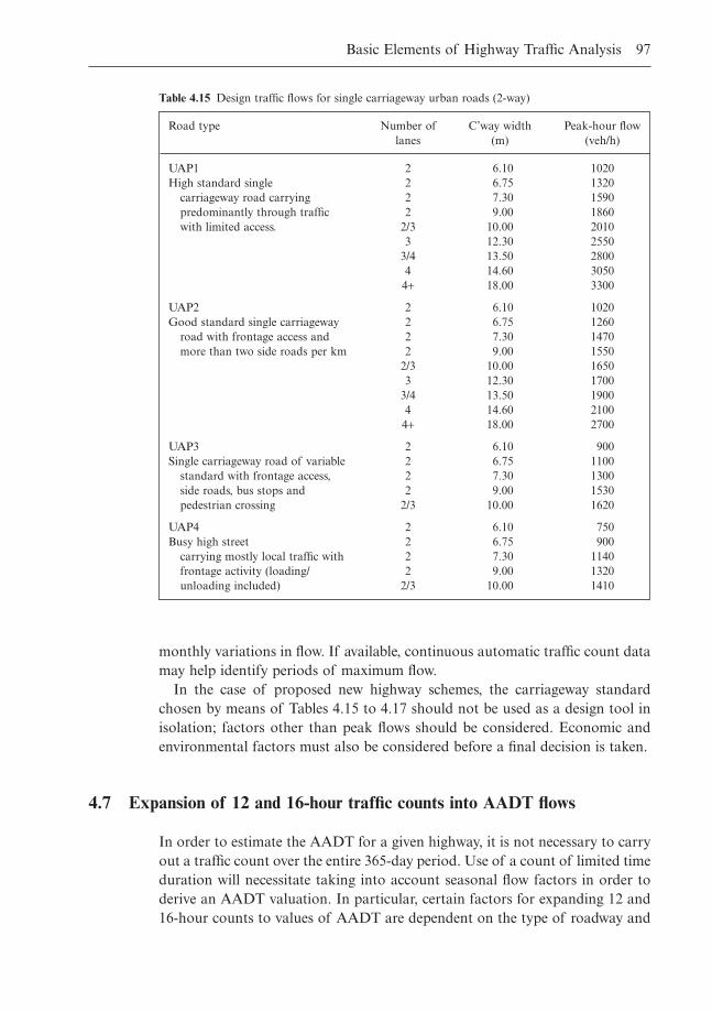
Basic Elements of Highway Traffic Analysis 97
Road type Number of C’way width Peak-hour flowlanes (m) (veh/h)
UAP1 2 6.10 1020High standard single 2 6.75 1320
carriageway road carrying 2 7.30 1590predominantly through traffic 2 9.00 1860with limited access. 2/3 10.00 2010
3 12.30 25503/4 13.50 28004 14.60 3050
4+ 18.00 3300
UAP2 2 6.10 1020Good standard single carriageway 2 6.75 1260
road with frontage access and 2 7.30 1470more than two side roads per km 2 9.00 1550
2/3 10.00 16503 12.30 1700
3/4 13.50 19004 14.60 2100
4+ 18.00 2700
UAP3 2 6.10 900Single carriageway road of variable 2 6.75 1100
standard with frontage access, 2 7.30 1300side roads, bus stops and 2 9.00 1530pedestrian crossing 2/3 10.00 1620
UAP4 2 6.10 750Busy high street 2 6.75 900
carrying mostly local traffic with 2 7.30 1140frontage activity (loading/ 2 9.00 1320unloading included) 2/3 10.00 1410
Table 4.15 Design traffic flows for single carriageway urban roads (2-way)
monthly variations in flow. If available, continuous automatic traffic count datamay help identify periods of maximum flow.
In the case of proposed new highway schemes, the carriageway standardchosen by means of Tables 4.15 to 4.17 should not be used as a design tool inisolation; factors other than peak flows should be considered. Economic andenvironmental factors must also be considered before a final decision is taken.
4.7 Expansion of 12 and 16-hour traffic counts into AADT flows
In order to estimate the AADT for a given highway, it is not necessary to carryout a traffic count over the entire 365-day period. Use of a count of limited timeduration will necessitate taking into account seasonal flow factors in order toderive an AADT valuation. In particular, certain factors for expanding 12 and16-hour counts to values of AADT are dependent on the type of roadway and
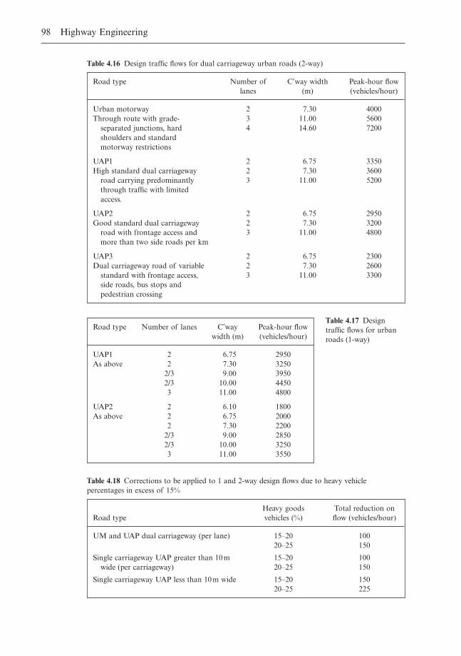
98 Highway Engineering
Road type Number of C’way width Peak-hour flowlanes (m) (vehicles/hour)
Urban motorway 2 7.30 4000Through route with grade- 3 11.00 5600
separated junctions, hard 4 14.60 7200shoulders and standardmotorway restrictions
UAP1 2 6.75 3350High standard dual carriageway 2 7.30 3600
road carrying predominantly 3 11.00 5200through traffic with limited access.
UAP2 2 6.75 2950Good standard dual carriageway 2 7.30 3200
road with frontage access and 3 11.00 4800more than two side roads per km
UAP3 2 6.75 2300Dual carriageway road of variable 2 7.30 2600
standard with frontage access, 3 11.00 3300side roads, bus stops and pedestrian crossing
Table 4.16 Design traffic flows for dual carriageway urban roads (2-way)
Road type Number of lanes C’way Peak-hour flowwidth (m) (vehicles/hour)
UAP1 2 6.75 2950As above 2 7.30 3250
2/3 9.00 39502/3 10.00 44503 11.00 4800
UAP2 2 6.10 1800As above 2 6.75 2000
2 7.30 22002/3 9.00 28502/3 10.00 32503 11.00 3550
Table 4.17 Designtraffic flows for urbanroads (1-way)
Heavy goods Total reduction onRoad type vehicles (%) flow (vehicles/hour)
UM and UAP dual carriageway (per lane) 15–20 10020–25 150
Single carriageway UAP greater than 10m 15–20 100wide (per carriageway) 20–25 150
Single carriageway UAP less than 10m wide 15–20 15020–25 225
Table 4.18 Corrections to be applied to 1 and 2-way design flows due to heavy vehiclepercentages in excess of 15%
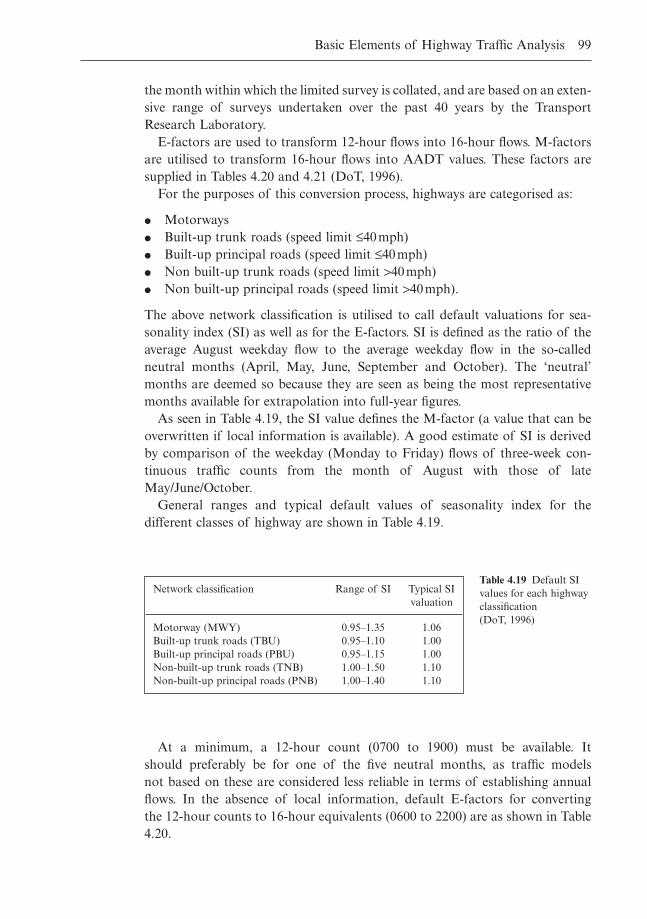
the month within which the limited survey is collated, and are based on an exten-sive range of surveys undertaken over the past 40 years by the TransportResearch Laboratory.
E-factors are used to transform 12-hour flows into 16-hour flows. M-factorsare utilised to transform 16-hour flows into AADT values. These factors aresupplied in Tables 4.20 and 4.21 (DoT, 1996).
For the purposes of this conversion process, highways are categorised as:
� Motorways� Built-up trunk roads (speed limit £40mph)� Built-up principal roads (speed limit £40mph)� Non built-up trunk roads (speed limit >40mph)� Non built-up principal roads (speed limit >40mph).
The above network classification is utilised to call default valuations for sea-sonality index (SI) as well as for the E-factors. SI is defined as the ratio of theaverage August weekday flow to the average weekday flow in the so-calledneutral months (April, May, June, September and October). The ‘neutral’months are deemed so because they are seen as being the most representativemonths available for extrapolation into full-year figures.
As seen in Table 4.19, the SI value defines the M-factor (a value that can beoverwritten if local information is available). A good estimate of SI is derivedby comparison of the weekday (Monday to Friday) flows of three-week con-tinuous traffic counts from the month of August with those of lateMay/June/October.
General ranges and typical default values of seasonality index for the different classes of highway are shown in Table 4.19.
Basic Elements of Highway Traffic Analysis 99
Network classification Range of SI Typical SI valuation
Motorway (MWY) 0.95–1.35 1.06Built-up trunk roads (TBU) 0.95–1.10 1.00Built-up principal roads (PBU) 0.95–1.15 1.00Non-built-up trunk roads (TNB) 1.00–1.50 1.10Non-built-up principal roads (PNB) 1.00–1.40 1.10
Table 4.19 Default SIvalues for each highwayclassification (DoT, 1996)
At a minimum, a 12-hour count (0700 to 1900) must be available. It should preferably be for one of the five neutral months, as traffic models not based on these are considered less reliable in terms of establishing annualflows. In the absence of local information, default E-factors for converting the 12-hour counts to 16-hour equivalents (0600 to 2200) are as shown in Table4.20.
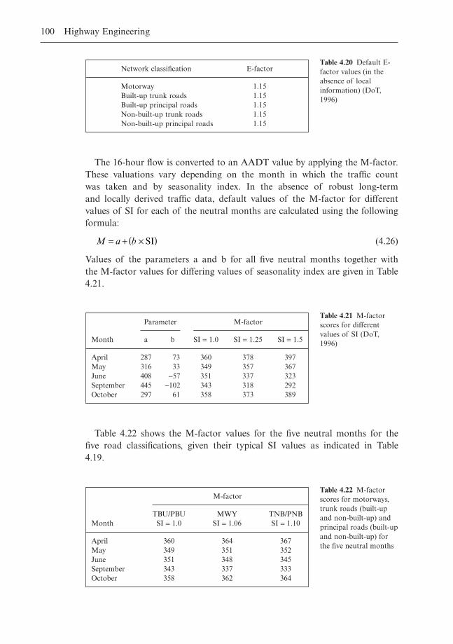
The 16-hour flow is converted to an AADT value by applying the M-factor.These valuations vary depending on the month in which the traffic count was taken and by seasonality index. In the absence of robust long-term and locally derived traffic data, default values of the M-factor for differentvalues of SI for each of the neutral months are calculated using the followingformula:
(4.26)
Values of the parameters a and b for all five neutral months together with the M-factor values for differing values of seasonality index are given in Table4.21.
M a b= + ¥( )SI
100 Highway Engineering
Network classification E-factor
Motorway 1.15Built-up trunk roads 1.15Built-up principal roads 1.15Non-built-up trunk roads 1.15Non-built-up principal roads 1.15
Table 4.20 Default E-factor values (in theabsence of localinformation) (DoT,1996)
Parameter M-factor
Month a b SI = 1.0 SI = 1.25 SI = 1.5
April 287 73 360 378 397May 316 33 349 357 367June 408 -57 351 337 323September 445 -102 343 318 292October 297 61 358 373 389
Table 4.21 M-factorscores for differentvalues of SI (DoT,1996)
Table 4.22 shows the M-factor values for the five neutral months for the five road classifications, given their typical SI values as indicated in Table 4.19.
M-factor
TBU/PBU MWY TNB/PNBMonth SI = 1.0 SI = 1.06 SI = 1.10
April 360 364 367May 349 351 352June 351 348 345September 343 337 333October 358 362 364
Table 4.22 M-factorscores for motorways,trunk roads (built-upand non-built-up) andprincipal roads (built-upand non-built-up) forthe five neutral months
Basic Elements of Highway Traffic Analysis 101
Example 4.8A 12-hour traffic count carried out on the route of a proposed motorway inApril established a volume of 45000 vehicles.What is the AADT figure?
Solution
Use E-factor to convert 12-hour value to a 16-hour value
45000 ¥ 1.15 = 51750
Use M-factor to convert 16-hour figure to AADTFor a motorway, with the traffic count taken in April, the M-factor is 364
Therefore,
Annual traffic = 51750 ¥ 364Annual average daily traffic = 51750 ¥ 364 ∏ 365 = 51608 vehicles.
This flow falls within the range of a 3-lane dual motorway (D3M).
4.8 Concluding comments
The British and American methods offer contrasting methodologies for sizinga roadway. The UK system yields a recommended design range which will offerthe designer a choice of types and widths. The final choice of option is madeby considering economic factors such as user travel and accident costs within acost-benefit framework. Environmental effects will also form part of the evalu-ation. The US system, on the other hand, relates design flows to the expectedlevel of service to be supplied by the highway. Level of service is dependent onfactors such as traffic speed and density.
4.9 References
Department of Transport (1985) Traffic flows and carriageway width assessments. Depart-mental Standard TD 20/85. The Stationery Office, London, UK.
Department of Transport (1996) Traffic Input to COBA. Design Manual for Roads andBridges, Volume 13: Economic Assessment of Roads. The Stationery Office, London,UK.
Department of Transport (1997a) Traffic Flow Ranges for Use in the Assessment of NewRural Road. Departmental Advice Note TA 46/97. The Stationery Office, London, UK.
Department of Transport (1997b) The COBA Manual. Design Manual for Roads andBridges, Volume 13: Economic Assessment of Roads. The Stationery Office, London,UK.

Department of Transport (1999) Traffic Capacity for Urban Roads. Departmental AdviceNote TA 79/99. The Stationery Office, UK.
Greenberg, H. (1959) Analysis of traffic flow. Operations Research, Volume 7, Number1.
Greenshields, B.D. (1934) A study of traffic capacity. Proceedings of the 14th AnnualMeeting of the Highway Research Board. Highway Research Board, Washington,District of Columbia, USA.
Pipes, L.A. (1967) Car following diagrams and the fundamental diagram of road traffic.Transport Research, 1, (1).
TRB (1985) Highway Capacity Manual. Special Report 209. Transportation ResearchBoard, Washington, District of Columbia, USA.
Underwood, R.T. (1961) Speed, volume and density relationships. In Quality and Theoryof Traffic Flow. Bureau of Highway Traffic, Yale, USA.
Werner, A. & Morrall, J.F. (1976) Passenger car equivalences of trucks, buses and recre-ational vehicles for two-lane rural highways. Transportation Research Record 615.
102 Highway Engineering
Chapter 5
The Design of Highway Intersections
5.1 Introduction
A highway intersection is required to control conflicting and merging streamsof traffic so that delay is minimised. This is achieved through choice of geo-metric parameters that control and regulate the vehicle paths through the intersection. These determine priority so that all movements take place withsafety.
The three main types of junction dealt with in this chapter are:
� Priority intersections, either simple T-junctions, staggered T-junctions orcrossroads
� Signalised intersections� Roundabouts.
All aim to provide vehicle drivers with a road layout that will minimise confu-sion. The need for flexibility dictates the choice of most suitable junction type.The selection process requires the economic, environmental and operationaleffects of each proposed option to be evaluated.
The assessment process requires the determination of the projected trafficflow at the location in question, termed the design reference flow. The rangewithin which this figure falls will indicate a junction design which is both eco-nomically and operationally efficient rather than one where there is either grossover or underprovision. Different combinations of turning movements shouldbe tested in order to check the performance characteristics of each junctionoption under consideration.
The starting point for any junction design is thus the determination of thevolume of traffic incident on it together with the various turning, merging andconflicting movements involved. The basis for the design will be the flow esti-mate for some point in the future – the design reference flow (DRF). It is anhourly flow rate. Anything from the highest annual hourly flow to the fiftiethhighest hourly flow can be used. For urban roads, use of the thirtieth highestflow is usual, with the fiftieth highest used on interurban routes.
Use of these figures implies that, during the design year in question, it can beanticipated that the design reference flow at the junction will be exceeded and a
certain level of congestion experienced. If, however, the highest hourly flow wasutilised, while no overcapacity will be experienced, the junction will operate atwell below its capacity for a large proportion of the time, thus making such adesign economically undesirable with its scale also having possible negative envi-ronmental effects due to the intrusion resulting from its sheer scale. (If the junc-tion is already in existence then the DRF can be determined by manual countsnoting both the composition of the traffic and all turning movements.)
5.2 Deriving design reference flows from baseline traffic figures
5.2.1 Existing junctions
At existing junctions, it will be possible to directly estimate peak hour and dailytraffic flows together with all turning movements. In order for the measurementsto be as representative as possible of general peak flow levels, it is desirable totake them during a normal weekday (Monday to Thursday) within a neutralmonth (April, May, June, September or October). Factoring up the observedmorning and evening peak hour flows using indices given in the National RoadTraffic Forecasts can lead to the derivation of DRFs for the design year (nor-mally 15 years after opening). Flow patterns and turning proportions observedin the base year can be extrapolated in order to predict future patterns ofmovement.
5.2.2 New junctions
In a situation where a junction is being designed for a new road or where flowpatterns through an existing junction are predicted to change significantlybecause of changes to the general network, flows must be derived by use of atraffic modelling process which will generate estimates of 12, 16 or 24 hour linkflows for a future chosen design year. AADT flows are then obtained by fac-toring the 12, 16 or 24 hour flows. The AAHT is then calculated (AADT ∏ 24)and then factored to represent the appropriate highest hourly flow using derivedfactors. Tidal flow is then taken into consideration; generally a 60/40 split infavour of the peak hour direction is assumed. Turning proportions are alsoguesstimated so that the junction can be designed.
5.2.3 Short-term variations in flow
Traffic does not usually arrive at a junction at a uniform or constant rate. Duringcertain periods, traffic may arrive at a rate higher than the DRF, at other periods lower. If the junction analysis for a priority junction/roundabout is
104 Highway Engineering
being done with the aid of one of the Transport Research Laboratory’s computer programs (PICADY/ARCADY), such variations can be allowed for using a ‘flow profile’. A typical profile could involve the inputting of peak-time flows in 15-minute intervals. When calculations are being completed by hand for a priority junction/roundabout, such short-term variations may be taken into consideration by utilising an hourly flow equal to 1.125 times theDRF.
In the case of a priority junction, this adjustment should be applied to thedesign flows on both the minor and major arms. In the case of a roundaboutintersection, this factored flow will impact not only on the entry flows to theroundabout but also the circulating flows within the intersection.
5.2.4 Conversion of AADT to highest hourly flows
Appendix D14 of the Traffic Appraisal Manual (DoT, 1996) originally detailedfactors linking AADT to the tenth, thirtieth, fiftieth, hundredth and two hun-dredth highest annual hourly peak flow for three classes of roads:
� Main urban� Interurban� Recreational interurban.
Particularly on urban highways, where peaks are less marked, the thirtiethhighest flow may be most appropriate. On an interurban route, the fiftiethhighest might apply. On recreational routes where peaks occur infrequently, thetwo hundredth highest may be the value most consistent with economic viabil-ity. The general implication is that where the design flow is exceeded some degreeof congestion will result, but this is preferable and economically more justifiableto the situation where congestion will never occur and the road is under capac-ity at all times.
The values originally given in Table 5A of Appendix D14 of the TrafficAppraisal Manual range between approximately 2.4 and 4.4. The use of thesenational expansion figures for converting AADT to peak hour flows is no longerrecommended. Rather it is advised that local traffic data be used in order tocompile such factors.
5.3 Major/minor priority intersections
5.3.1 Introduction
A priority intersection occurs between two roads, one termed the ‘major’ roadand the other the ‘minor’ road. The major road is the one assigned a permanentpriority of traffic movement over that of the minor road. The minor road must
The Design of Highway Intersections 105
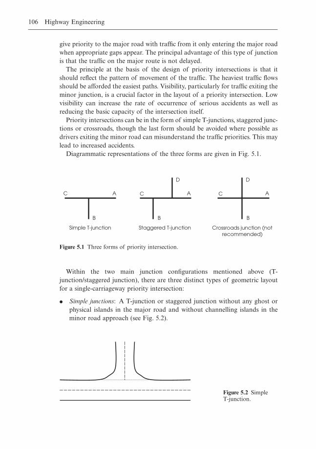
give priority to the major road with traffic from it only entering the major roadwhen appropriate gaps appear. The principal advantage of this type of junctionis that the traffic on the major route is not delayed.
The principle at the basis of the design of priority intersections is that itshould reflect the pattern of movement of the traffic. The heaviest traffic flowsshould be afforded the easiest paths. Visibility, particularly for traffic exiting theminor junction, is a crucial factor in the layout of a priority intersection. Lowvisibility can increase the rate of occurrence of serious accidents as well asreducing the basic capacity of the intersection itself.
Priority intersections can be in the form of simple T-junctions, staggered junc-tions or crossroads, though the last form should be avoided where possible asdrivers exiting the minor road can misunderstand the traffic priorities. This maylead to increased accidents.
Diagrammatic representations of the three forms are given in Fig. 5.1.
106 Highway Engineering
Simple T-junction Staggered T-junction Crossroads junction (not recommended)
AC
B
AC
B
D
A C
B
D
Figure 5.1 Three forms of priority intersection.
Within the two main junction configurations mentioned above (T-junction/staggered junction), there are three distinct types of geometric layoutfor a single-carriageway priority intersection:
� Simple junctions: A T-junction or staggered junction without any ghost orphysical islands in the major road and without channelling islands in theminor road approach (see Fig. 5.2).
Figure 5.2 Simple T-junction.
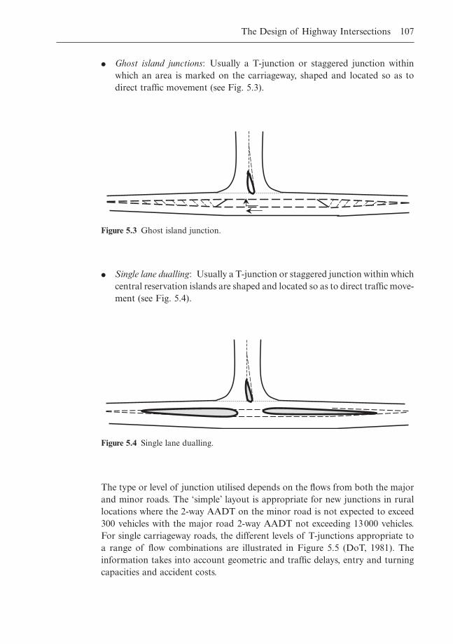
� Ghost island junctions: Usually a T-junction or staggered junction withinwhich an area is marked on the carriageway, shaped and located so as todirect traffic movement (see Fig. 5.3).
The Design of Highway Intersections 107
Figure 5.3 Ghost island junction.
Figure 5.4 Single lane dualling.
The type or level of junction utilised depends on the flows from both the majorand minor roads. The ‘simple’ layout is appropriate for new junctions in rurallocations where the 2-way AADT on the minor road is not expected to exceed300 vehicles with the major road 2-way AADT not exceeding 13000 vehicles.For single carriageway roads, the different levels of T-junctions appropriate toa range of flow combinations are illustrated in Figure 5.5 (DoT, 1981). Theinformation takes into account geometric and traffic delays, entry and turningcapacities and accident costs.
� Single lane dualling: Usually a T-junction or staggered junction within whichcentral reservation islands are shaped and located so as to direct traffic move-ment (see Fig. 5.4).
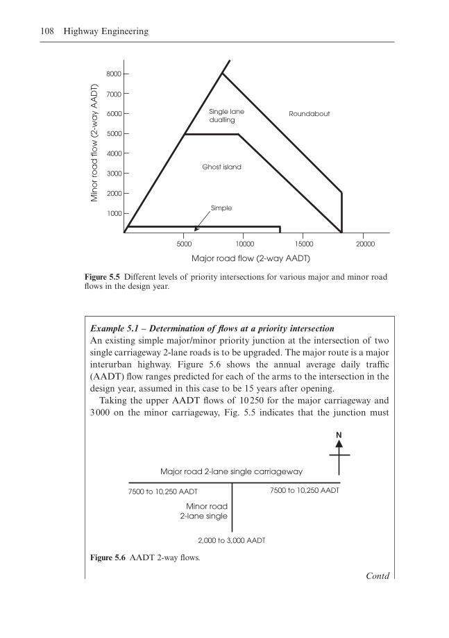
108 Highway Engineering
Ghost island
Single lane dualling
Simple
Roundabout
8000
7000
6000
5000
4000
3000
2000
1000
100005000 15000 20000
Min
or r
oa
d f
low
(2-
wa
y A
AD
T)
Major road flow (2-way AADT)
Figure 5.5 Different levels of priority intersections for various major and minor roadflows in the design year.
Example 5.1 – Determination of flows at a priority intersectionAn existing simple major/minor priority junction at the intersection of twosingle carriageway 2-lane roads is to be upgraded. The major route is a majorinterurban highway. Figure 5.6 shows the annual average daily traffic(AADT) flow ranges predicted for each of the arms to the intersection in thedesign year, assumed in this case to be 15 years after opening.
Taking the upper AADT flows of 10250 for the major carriageway and 3000 on the minor carriageway, Fig. 5.5 indicates that the junction must
7500 to 10,250 AADT
Minor road2-lane single
Major road 2-lane single carriageway
7500 to 10,250 AADT
2,000 to 3,000 AADT
N
Figure 5.6 AADT 2-way flows.
Contd
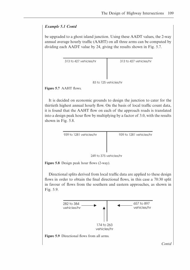
The Design of Highway Intersections 109
Example 5.1 Contd
be upgraded to a ghost island junction. Using these AADT values, the 2-wayannual average hourly traffic (AAHT) on all three arms can be computed bydividing each AADT value by 24, giving the results shown in Fig. 5.7.
313 to 427 vehicles/hr
83 to 125 vehicles/hr
313 to 427 vehicles/hr
Figure 5.7 AAHT flows.
It is decided on economic grounds to design the junction to cater for thethirtieth highest annual hourly flow. On the basis of local traffic count data,it is found that the AAHT flow on each of the approach roads is translatedinto a design peak hour flow by multiplying by a factor of 3.0, with the resultsshown in Fig. 5.8.
939 to 1281 vehicles/hr
249 to 375 vehicles/hr
939 to 1281 vehicles/hr
Figure 5.8 Design peak hour flows (2-way).
Directional splits derived from local traffic data are applied to these designflows in order to obtain the final directional flows, in this case a 70:30 splitin favour of flows from the southern and eastern approaches, as shown inFig. 5.9.
282 to 384 vehicles/hr
174 to 263 vehicles/hr
657 to 897 vehicles/hr
Figure 5.9 Directional flows from all arms.
Contd
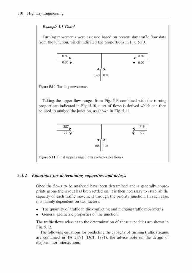
5.3.2 Equations for determining capacities and delays
Once the flows to be analysed have been determined and a generally appro-priate geometric layout has been settled on, it is then necessary to establish thecapacity of each traffic movement through the priority junction. In each case,it is mainly dependent on two factors:
� The quantity of traffic in the conflicting and merging traffic movements� General geometric properties of the junction.
The traffic flows relevant to the determination of these capacities are shown inFig. 5.12.
The following equations for predicting the capacity of turning traffic streamsare contained in TA 23/81 (DoT, 1981), the advice note on the design ofmajor/minor intersections:
110 Highway Engineering
Example 5.1 Contd
Turning movements were assessed based on present day traffic flow datafrom the junction, which indicated the proportions in Fig. 5.10.
0.80
0.20
0.400.60
0.80
0.20
Figure 5.10 Turning movements.
Taking the upper flow ranges from Fig. 5.9, combined with the turningproportions indicated in Fig. 5.10, a set of flows is derived which can thenbe used to analyse the junction, as shown in Fig. 5.11.
307
77
105158
718
179
Figure 5.11 Final upper range flows (vehicles per hour).
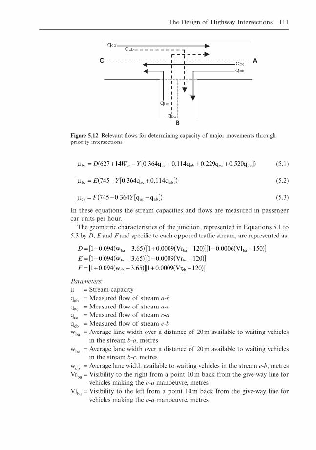
(5.1)
(5.2)
(5.3)
In these equations the stream capacities and flows are measured in passengercar units per hour.
The geometric characteristics of the junction, represented in Equations 5.1 to5.3 by D, E and F and specific to each opposed traffic stream, are represented as:
Parameters:m = Stream capacityqab = Measured flow of stream a-bqac = Measured flow of stream a-cqca = Measured flow of stream c-aqcb = Measured flow of stream c-bwba = Average lane width over a distance of 20m available to waiting vehicles
in the stream b-a, metreswbc = Average lane width over a distance of 20m available to waiting vehicles
in the stream b-c, metreswcb = Average lane width available to waiting vehicles in the stream c-b, metresVrba = Visibility to the right from a point 10m back from the give-way line for
vehicles making the b-a manoeuvre, metresVlba = Visibility to the left from a point 10m back from the give-way line for
vehicles making the b-a manoeuvre, metres
D
E
F
= + -( )[ ] + -( )[ ] + -( )[ ]= + -( )[ ] + -( )[ ]= + -( )[ ] + -( )[ ]
1 0 094 3 65 1 0 0009 120 1 0 0006 150
1 0 094 3 65 1 0 0009 120
1 0 094 3 65 1 0 0009 120
. . . .
. . .
. . .
w Vr Vl
w Vr
w Vr
ba ba ba
bc bc
cb cb
mcb ac abq q= - +[ ]( )F Y745 0 364.
mbc ac abq q= - +[ ]( )E Y745 0 364 0 114. .
mba cr ac ab ca cbq q q q= + - + + +[ ]( )D W Y627 14 0 364 0 114 0 229 0 520. . . .
The Design of Highway Intersections 111
Bqba
qac qab
qcb qca
qbc
C A
Figure 5.12 Relevant flows for determining capacity of major movements throughpriority intersections.
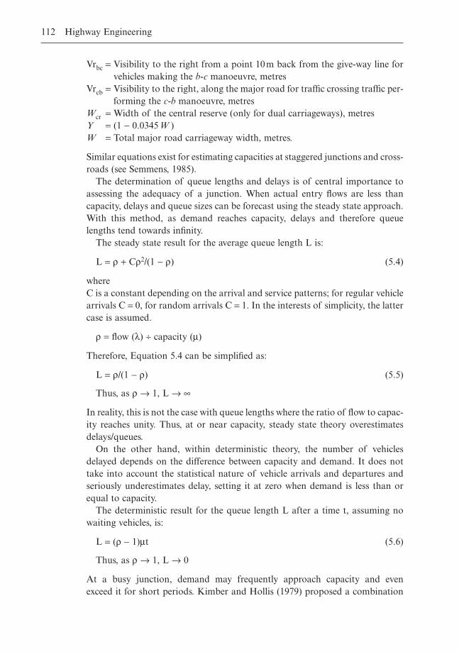
Vrbc = Visibility to the right from a point 10m back from the give-way line forvehicles making the b-c manoeuvre, metres
Vrcb = Visibility to the right, along the major road for traffic crossing traffic per-forming the c-b manoeuvre, metres
Wcr = Width of the central reserve (only for dual carriageways), metresY = (1 - 0.0345W )W = Total major road carriageway width, metres.
Similar equations exist for estimating capacities at staggered junctions and cross-roads (see Semmens, 1985).
The determination of queue lengths and delays is of central importance toassessing the adequacy of a junction. When actual entry flows are less thancapacity, delays and queue sizes can be forecast using the steady state approach.With this method, as demand reaches capacity, delays and therefore queuelengths tend towards infinity.
The steady state result for the average queue length L is:
L = r + Cr2/(1 - r) (5.4)
whereC is a constant depending on the arrival and service patterns; for regular vehiclearrivals C = 0, for random arrivals C = 1. In the interests of simplicity, the lattercase is assumed.
r = flow (l) ∏ capacity (m)
Therefore, Equation 5.4 can be simplified as:
L = r/(1 - r) (5.5)
Thus, as r Æ 1, L Æ •
In reality, this is not the case with queue lengths where the ratio of flow to capac-ity reaches unity. Thus, at or near capacity, steady state theory overestimatesdelays/queues.
On the other hand, within deterministic theory, the number of vehiclesdelayed depends on the difference between capacity and demand. It does nottake into account the statistical nature of vehicle arrivals and departures andseriously underestimates delay, setting it at zero when demand is less than orequal to capacity.
The deterministic result for the queue length L after a time t, assuming nowaiting vehicles, is:
L = (r - 1)mt (5.6)
Thus, as r Æ 1, L Æ 0
At a busy junction, demand may frequently approach capacity and even exceed it for short periods. Kimber and Hollis (1979) proposed a combination
112 Highway Engineering
of Equations 5.5 and 5.6, using co-ordinate transformations to derive the fol-lowing equations for average queue length and delay.
Queue length
L = 0.5 ¥ ((A2 + B)1/2 - A) (5.7)
where
(5.8)
(5.9)
Delay per unit time
Kimber and Hollis (1979) evaluated the relevant area under the queue lengthcurve in order to derive an expression for delay.
(5.10)
where
(5.11)
(5.12)
Delay per arriving vehicle
Kimber and Hollis (1979) derived the following expression as a measure of theaverage delay per arriving vehicle over an interval. The expression has two parts;the first relates to those suffered in the queue while the second (1/m) relates tothose encountered at the give-way line.
(5.13)
where
(5.14)
(5.15)QCt L
t0= +Ê
ËÁˆ¯̃
2 2m
rm
P t L C0= ¥ -( )[ ] - -( )0 5 11
. rm
D P Q) P)2v = ¥ + - +0 5 11 2. (( m
GL t t C L t
t +2 1 C0 0=
+( ) - -( ) +( )Î ˚-( )
2 2 1 2rm m rmm
Ft L t C L t
t +2 1 C0 0=
-( )( ) - -( ) - -( ) +( )-( )( )
1 2 1 4 12
2r m m rmm
D F G) F)2 1 2t = ¥ + -0 5. ((
BL t t C L t
t C0 0=
+( ) - -( ) +( )Î ˚+ -( )
4 11
rm m rmm
A =1 t L t C L t
t C0 0-( )( ) + -( ) - -( ) +( )+ -( )
r m m rmm
2 1 2 11
The Design of Highway Intersections 113
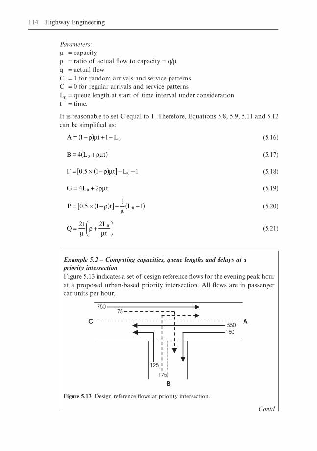
Parameters:m = capacityr = ratio of actual flow to capacity = q/mq = actual flowC = 1 for random arrivals and service patternsC = 0 for regular arrivals and service patternsL0 = queue length at start of time interval under considerationt = time.
It is reasonable to set C equal to 1. Therefore, Equations 5.8, 5.9, 5.11 and 5.12can be simplified as:
(5.16)
(5.17)
(5.18)
(5.19)
(5.20)
(5.21)Qt L
t= +Ê
ËÁˆ¯̃
2 2 0
mr
m
P t L0= ¥ -( )[ ] - -( )0 5 11
1. rm
G L t0= +4 2rm
F t L0= ¥ -( )[ ] - +0 5 1 1. r m
B = 4 L t0 +( )rm
A = 1 t L0-( ) + -r m 1
114 Highway Engineering
Example 5.2 – Computing capacities, queue lengths and delays at a priority intersectionFigure 5.13 indicates a set of design reference flows for the evening peak hourat a proposed urban-based priority intersection. All flows are in passengercar units per hour.
175
B
550 150
75 750
125
C A
Figure 5.13 Design reference flows at priority intersection.
Contd
The Design of Highway Intersections 115
Example 5.2 Contd
Estimate the ratio of flow to capacity for each of the opposed movementsand, for the one with the highest ratio, estimate the average queue length anddelay per vehicle during the peak hour.
Geometric parameters:
The width of the major carriageway (W) is 9.5m.
The lane widths for traffic exiting the minor road turning both left and right(wba, wbc) are 2.5m.
The lane width on the major road for traffic waiting to turn right onto theminor road (wcb), is 2.2m.
Visibility to the right and left for traffic exiting the minor road turning right(Vrba, Vlba) is 30m and 50m respectively.
Visibility to the right for traffic exiting the minor road turning left (Vrbc) is30m.
Visibility to the right for traffic exiting the major road, turning right onto theminor road (Vrcb) is 50m.
Solution
When using Equations 5.1 to 5.3 for estimating the ratios of flow to capac-ity for the various opposed turning movements, the design reference flowsshown in Fig. 5.13 should be multiplied by 1.125 in order to allow for short-term variations in the traffic flow. (These short-term variations are allowedfor in PICADY.)
Factored flows:qab = 169 (150 ¥ 1.125)
qac = 619 (550 ¥ 1.125)
qca = 844 (750 ¥ 1.125)
qcb = 84 (75 ¥ 1.125)
qba = 197 (175 ¥ 1.125)
qbc = 141 (125 ¥ 1.125)
Contd
116 Highway Engineering
Example 5.2 Contd
Parameters D, E and F:
Capacities:
m
m
m
ba
bc
cb
pcu/hr
pcu/hr
pcu/hr
= - ( ) + ( ) + ( ) + ( )[ ]{ }== - ( )( ) + ( )[ ]{ }== - ¥( ) +( )[ ]=
0 77 627 0 67 0 364 619 0 114 169 0 229 844 0 520 84
234
0 82 745 0 67 0 364 619 0 114 169
477
0 81 745 0 364 0 67 619 169
448
. . . . . .
. . . .
. . .
D
E
F
Y
= + -( )[ ] + -( )[ ] + -( )[ ] == + -( )[ ] + -( )[ ] == + -( )[ ] + -( )[ ] =
1 0 094 2 5 3 65 1 0 0009 30 120 1 0 0006 50 150 0 77
1 0 094 2 5 3 65 1 0 0009 30 120 0 82
1 0 094 2 2 36 5 1 0 0009 50 120 0 81
. . . . . .
. . . . .
. . . . .
== - ¥( )( )[ ] =1 0 345 9 5 0 67. . .
Ratios of flow to capacity (RFC):For the most critical movement (traffic exiting onto the major road, turning
right) the ratio is just below the maximum allowed in urban areas of 0.85.The maximum reduces to 0.75 in rural areas.
Stream Flow (pcu/hr) Capacity (pcu/hr) RFC
qba 197 234 0.84qbc 141 477 0.30qcb 84 448 0.19
Table 5.1 RFCs foropposed flowmovements
Queue length at stream B-A:
L = 0.5 ¥ ((A2 + B)1/2 - A)
Assuming random arrivals (therefore C = 1)
A = (1 - r)mt + 1 - L0B = 4(L0 + rmt)r = 0.84m = 234 pcu/hrt = 1 hourL0 = 0 (no cars waiting at start of time period)
Contd
Example 5.2 Contd
Therefore
Total delay during peak hour
Delay per arriving vehicle (excluding delay at stop-line)
Thus, the average delay per vehicle is 1.3 minutes, with a queue length of fivevehicles.
D P Q) P)+1
P
Q =2
234
D
hours
= 79 seconds per vehicle
2 1 2v
v
= ¥ + -
= ¥[ ]+
= +=
¥
== ¥ + -[ ]{ } +=
0 5
0 5 0 161
2340 08 0 00427
0 0843
0 84
0 0072
0 5 0 0843 0 0072 0 0843 1 234
0 0219
2 1 2
. ((
. .
. .
.
.
.
. ( . . ) .
.
m
D F G) F)
F
G
D
hours.
2 1 2t
t
= ¥ + -= ¥ -( ) ¥ ¥[ ]+== ¥ ¥ ¥== ¥ + -=
0 5
0 5 1 0 84 234 1 1
11 72
2 0 84 234 1
393 12
0 5 19 72 393 12 17 72
4 1
2 1 2
. (
. .
.
.
.
. (( . . ) . )
.
A
B
L
cars
= -( ) ¥ ¥[ ]+== ¥ ¥ ¥== ¥ + -=
1 0 84 234 1 1
38 44
4 0 84 234 1
786 24
0 5 38 44 786 24 32 45
5
2 1 2
.
.
.
.
. (( . . ) . )
The Design of Highway Intersections 117
5.3.3 Geometric layout details (DoT, 1995)
Horizontal alignment
In the ideal situation, the priority intersection should not be sited where themajor road is on a sharp curve. Where this is unavoidable, it is preferable thatthe T-junction is located with the minor junction on the outside of the curve.
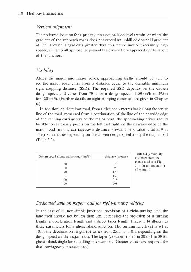
Vertical alignment
The preferred location for a priority intersection is on level terrain, or where thegradient of the approach roads does not exceed an uphill or downhill gradientof 2%. Downhill gradients greater than this figure induce excessively highspeeds, while uphill approaches prevent the drivers from appreciating the layoutof the junction.
Visibility
Along the major and minor roads, approaching traffic should be able to see the minor road entry from a distance equal to the desirable minimum sight stopping distance (SSD). The required SSD depends on the chosen design speed and varies from 70m for a design speed of 50km/h to 295m for 120km/h. (Further details on sight stopping distances are given in Chapter6.)
In addition, on the minor road, from a distance x metres back along the centreline of the road, measured from a continuation of the line of the nearside edgeof the running carriageway of the major road, the approaching driver shouldbe able to see clearly points on the left and right on the nearside edge of themajor road running carriageway a distance y away. The x value is set at 9m.The y value varies depending on the chosen design speed along the major road(Table 5.2).
118 Highway Engineering
Design speed along major road (km/h) y distance (metres)
50 7060 9070 12085 160
100 215120 295
Table 5.2 y visibilitydistances from theminor road (see Fig.5.14 for an illustrationof x and y)
Dedicated lane on major road for right-turning vehicles
In the case of all non-simple junctions, provision of a right-turning lane, thelane itself should not be less than 3m. It requires the provision of a turninglength, a deceleration length and a direct taper length. Figure 5.14 illustratesthese parameters for a ghost island junction. The turning length (a) is set at 10m; the deceleration length (b) varies from 25m to 110m depending on thedesign speed on the major route. The taper (c) varies from 1 in 20 to 1 in 30 forghost island/single lane dualling intersections. (Greater values are required fordual carriageway intersections.)
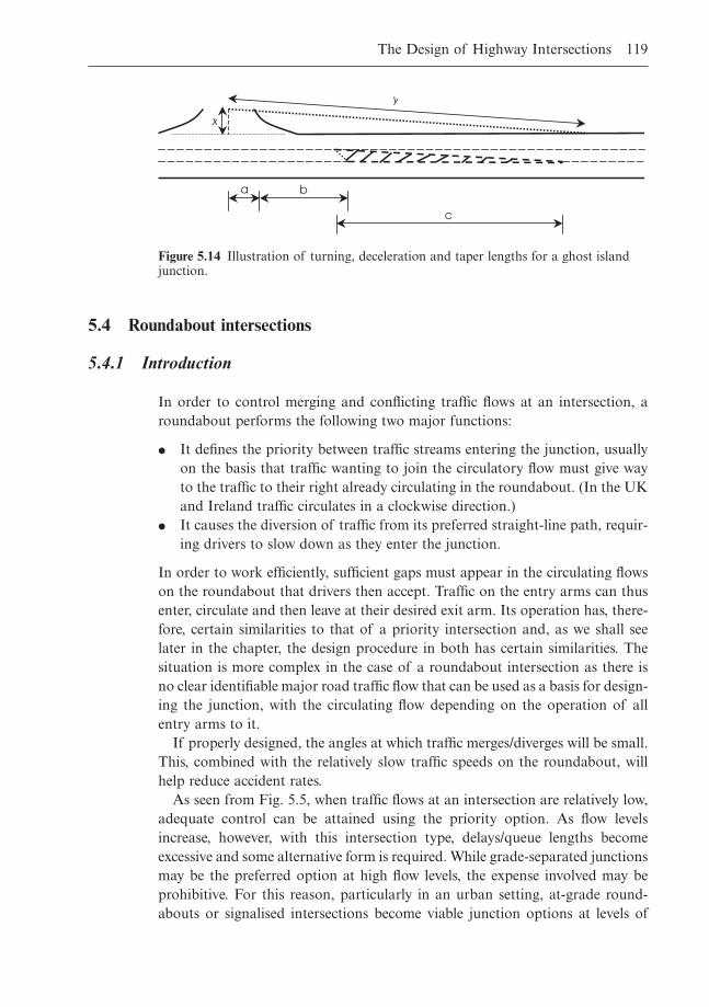
5.4 Roundabout intersections
5.4.1 Introduction
In order to control merging and conflicting traffic flows at an intersection, aroundabout performs the following two major functions:
� It defines the priority between traffic streams entering the junction, usuallyon the basis that traffic wanting to join the circulatory flow must give wayto the traffic to their right already circulating in the roundabout. (In the UKand Ireland traffic circulates in a clockwise direction.)
� It causes the diversion of traffic from its preferred straight-line path, requir-ing drivers to slow down as they enter the junction.
In order to work efficiently, sufficient gaps must appear in the circulating flowson the roundabout that drivers then accept. Traffic on the entry arms can thusenter, circulate and then leave at their desired exit arm. Its operation has, there-fore, certain similarities to that of a priority intersection and, as we shall seelater in the chapter, the design procedure in both has certain similarities. Thesituation is more complex in the case of a roundabout intersection as there isno clear identifiable major road traffic flow that can be used as a basis for design-ing the junction, with the circulating flow depending on the operation of allentry arms to it.
If properly designed, the angles at which traffic merges/diverges will be small.This, combined with the relatively slow traffic speeds on the roundabout, willhelp reduce accident rates.
As seen from Fig. 5.5, when traffic flows at an intersection are relatively low,adequate control can be attained using the priority option. As flow levelsincrease, however, with this intersection type, delays/queue lengths becomeexcessive and some alternative form is required. While grade-separated junctionsmay be the preferred option at high flow levels, the expense involved may beprohibitive. For this reason, particularly in an urban setting, at-grade round-abouts or signalised intersections become viable junction options at levels of
The Design of Highway Intersections 119
a b
c
y
x
Figure 5.14 Illustration of turning, deceleration and taper lengths for a ghost islandjunction.
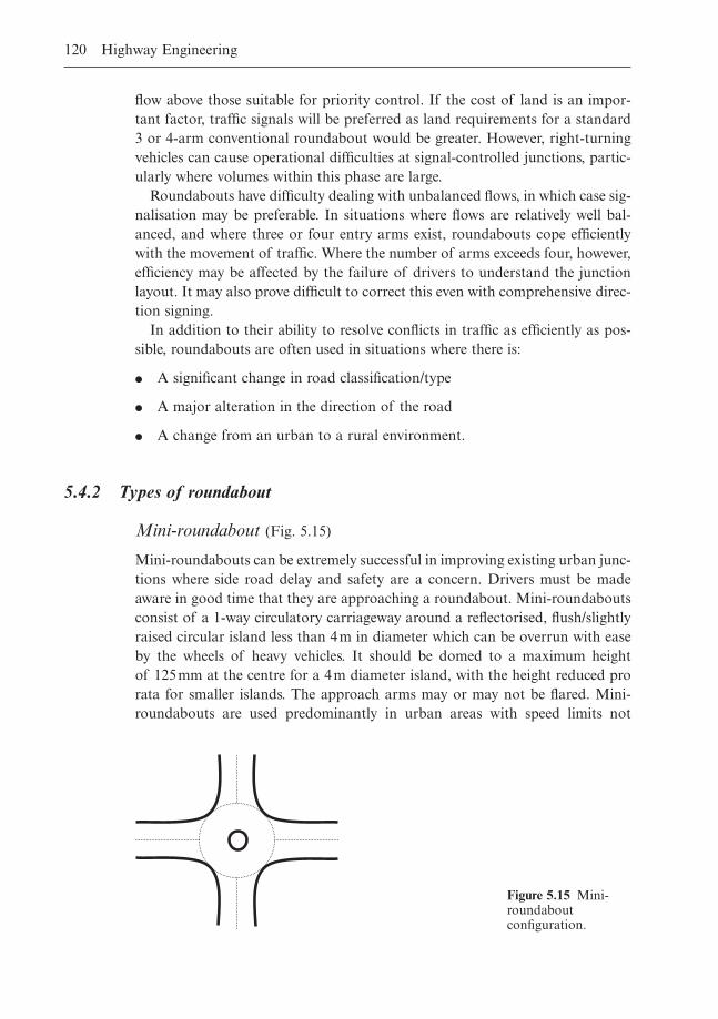
flow above those suitable for priority control. If the cost of land is an impor-tant factor, traffic signals will be preferred as land requirements for a standard3 or 4-arm conventional roundabout would be greater. However, right-turningvehicles can cause operational difficulties at signal-controlled junctions, partic-ularly where volumes within this phase are large.
Roundabouts have difficulty dealing with unbalanced flows, in which case sig-nalisation may be preferable. In situations where flows are relatively well bal-anced, and where three or four entry arms exist, roundabouts cope efficientlywith the movement of traffic. Where the number of arms exceeds four, however,efficiency may be affected by the failure of drivers to understand the junctionlayout. It may also prove difficult to correct this even with comprehensive direc-tion signing.
In addition to their ability to resolve conflicts in traffic as efficiently as pos-sible, roundabouts are often used in situations where there is:
� A significant change in road classification/type
� A major alteration in the direction of the road
� A change from an urban to a rural environment.
5.4.2 Types of roundabout
Mini-roundabout (Fig. 5.15)
Mini-roundabouts can be extremely successful in improving existing urban junc-tions where side road delay and safety are a concern. Drivers must be madeaware in good time that they are approaching a roundabout. Mini-roundaboutsconsist of a 1-way circulatory carriageway around a reflectorised, flush/slightlyraised circular island less than 4m in diameter which can be overrun with easeby the wheels of heavy vehicles. It should be domed to a maximum height of 125mm at the centre for a 4m diameter island, with the height reduced prorata for smaller islands. The approach arms may or may not be flared. Mini-roundabouts are used predominantly in urban areas with speed limits not
120 Highway Engineering
Figure 5.15 Mini-roundaboutconfiguration.
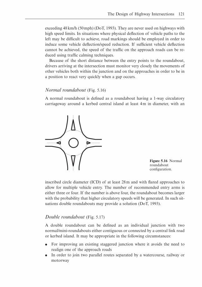
exceeding 48km/h (50mph) (DoT, 1993). They are never used on highways withhigh speed limits. In situations where physical deflection of vehicle paths to theleft may be difficult to achieve, road markings should be employed in order toinduce some vehicle deflection/speed reduction. If sufficient vehicle deflectioncannot be achieved, the speed of the traffic on the approach roads can be re-duced using traffic calming techniques.
Because of the short distance between the entry points to the roundabout,drivers arriving at the intersection must monitor very closely the movements ofother vehicles both within the junction and on the approaches in order to be ina position to react very quickly when a gap occurs.
Normal roundabout (Fig. 5.16)
A normal roundabout is defined as a roundabout having a 1-way circulatorycarriageway around a kerbed central island at least 4m in diameter, with an
The Design of Highway Intersections 121
Figure 5.16 Normalroundaboutconfiguration.
inscribed circle diameter (ICD) of at least 28m and with flared approaches toallow for multiple vehicle entry. The number of recommended entry arms iseither three or four. If the number is above four, the roundabout becomes largerwith the probability that higher circulatory speeds will be generated. In such sit-uations double roundabouts may provide a solution (DoT, 1993).
Double roundabout (Fig. 5.17)
A double roundabout can be defined as an individual junction with twonormal/mini-roundabouts either contiguous or connected by a central link roador kerbed island. It may be appropriate in the following circumstances:
� For improving an existing staggered junction where it avoids the need torealign one of the approach roads
� In order to join two parallel routes separated by a watercourse, railway ormotorway
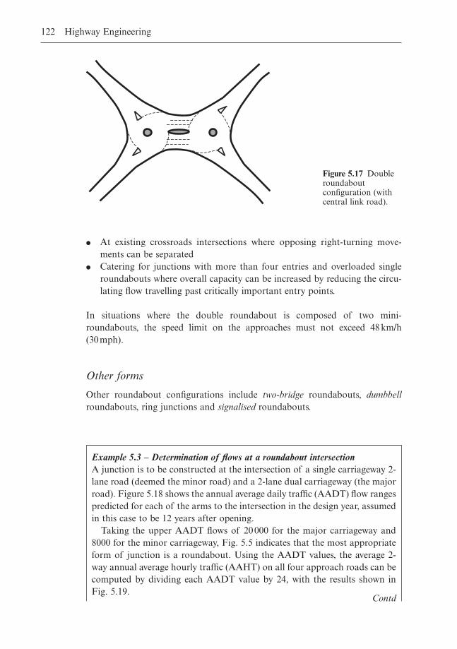
� At existing crossroads intersections where opposing right-turning move-ments can be separated
� Catering for junctions with more than four entries and overloaded singleroundabouts where overall capacity can be increased by reducing the circu-lating flow travelling past critically important entry points.
In situations where the double roundabout is composed of two mini-roundabouts, the speed limit on the approaches must not exceed 48km/h (30mph).
Other forms
Other roundabout configurations include two-bridge roundabouts, dumbbellroundabouts, ring junctions and signalised roundabouts.
122 Highway Engineering
Figure 5.17 Doubleroundaboutconfiguration (withcentral link road).
Example 5.3 – Determination of flows at a roundabout intersectionA junction is to be constructed at the intersection of a single carriageway 2-lane road (deemed the minor road) and a 2-lane dual carriageway (the majorroad). Figure 5.18 shows the annual average daily traffic (AADT) flow rangespredicted for each of the arms to the intersection in the design year, assumedin this case to be 12 years after opening.
Taking the upper AADT flows of 20000 for the major carriageway and8000 for the minor carriageway, Fig. 5.5 indicates that the most appropriateform of junction is a roundabout. Using the AADT values, the average 2-way annual average hourly traffic (AAHT) on all four approach roads can becomputed by dividing each AADT value by 24, with the results shown in Fig. 5.19.
Contd
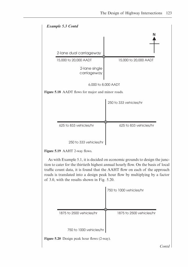
The Design of Highway Intersections 123
As with Example 5.1, it is decided on economic grounds to design the junc-tion to cater for the thirtieth highest annual hourly flow. On the basis of localtraffic count data, it is found that the AAHT flow on each of the approachroads is translated into a design peak hour flow by multiplying by a factorof 3.0, with the results shown in Fig. 5.20.
2-lane dual carriageway
2-lane singlecarriageway
15,000 to 20,000 AADT 15,000 to 20,000 AADT
6,000 to 8,000 AADT
N
Figure 5.18 AADT flows for major and minor roads.
625 to 833 vehicles/hr
250 to 333 vehicles/hr
625 to 833 vehicles/hr
250 to 333 vehicles/hr
Figure 5.19 AAHT 2-way flows.
Contd
Example 5.3 Contd
1875 to 2500 vehicles/hr
750 to 1000 vehicles/hr
1875 to 2500 vehicles/hr
750 to 1000 vehicles/hr
Figure 5.20 Design peak hour flows (2-way).
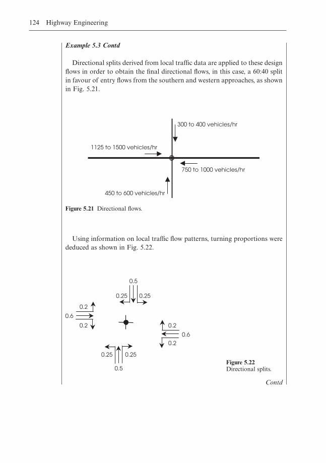
124 Highway Engineering
Example 5.3 Contd
Directional splits derived from local traffic data are applied to these designflows in order to obtain the final directional flows, in this case, a 60:40 splitin favour of entry flows from the southern and western approaches, as shownin Fig. 5.21.
1125 to 1500 vehicles/hr
450 to 600 vehicles/hr
750 to 1000 vehicles/hr
300 to 400 vehicles/hr
Figure 5.21 Directional flows.
0.2
0.6
0.2
0.5
0.25 0.25
0.6
0.2
0.2
0.5
0.250.25Figure 5.22Directional splits.
Using information on local traffic flow patterns, turning proportions werededuced as shown in Fig. 5.22.
Contd
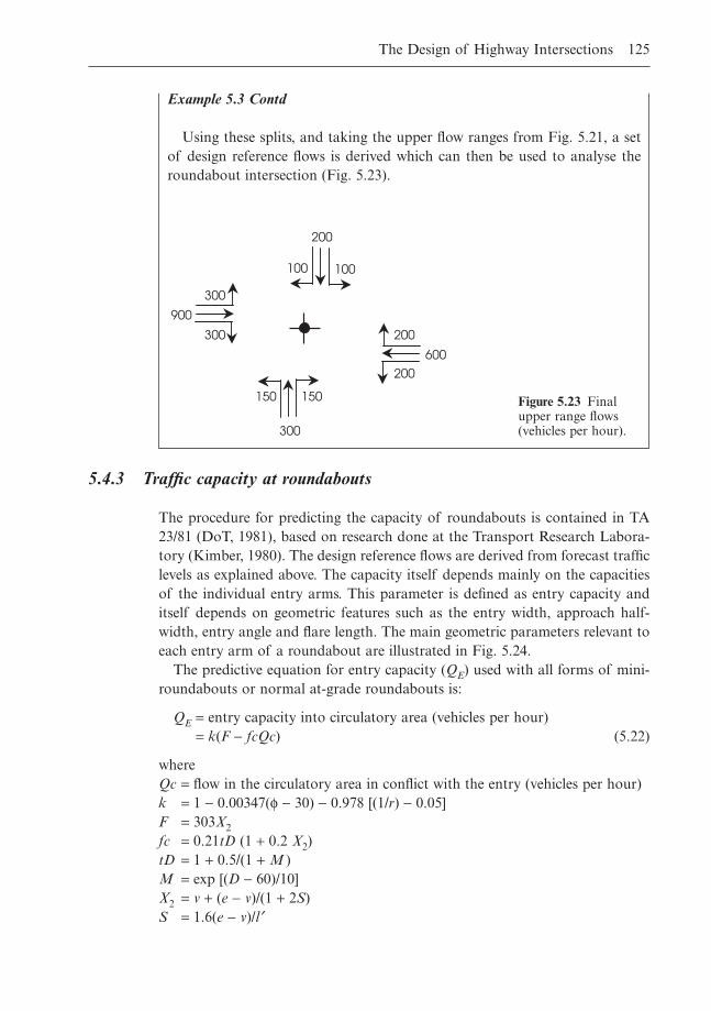
5.4.3 Traffic capacity at roundabouts
The procedure for predicting the capacity of roundabouts is contained in TA23/81 (DoT, 1981), based on research done at the Transport Research Labora-tory (Kimber, 1980). The design reference flows are derived from forecast trafficlevels as explained above. The capacity itself depends mainly on the capacitiesof the individual entry arms. This parameter is defined as entry capacity anditself depends on geometric features such as the entry width, approach half-width, entry angle and flare length. The main geometric parameters relevant toeach entry arm of a roundabout are illustrated in Fig. 5.24.
The predictive equation for entry capacity (QE) used with all forms of mini-roundabouts or normal at-grade roundabouts is:
QE = entry capacity into circulatory area (vehicles per hour)= k(F - fcQc) (5.22)
whereQc = flow in the circulatory area in conflict with the entry (vehicles per hour)k = 1 - 0.00347(f - 30) - 0.978 [(1/r) - 0.05]F = 303X2fc = 0.21tD (1 + 0.2 X2)tD = 1 + 0.5/(1 + M )M = exp [(D - 60)/10]X2 = v + (e - v)/(1 + 2S)S = 1.6(e - v)/l¢
The Design of Highway Intersections 125
Example 5.3 Contd
Using these splits, and taking the upper flow ranges from Fig. 5.21, a setof design reference flows is derived which can then be used to analyse theroundabout intersection (Fig. 5.23).
100
200
100
300
900
300
600
200
200
300
150150 Figure 5.23 Finalupper range flows(vehicles per hour).
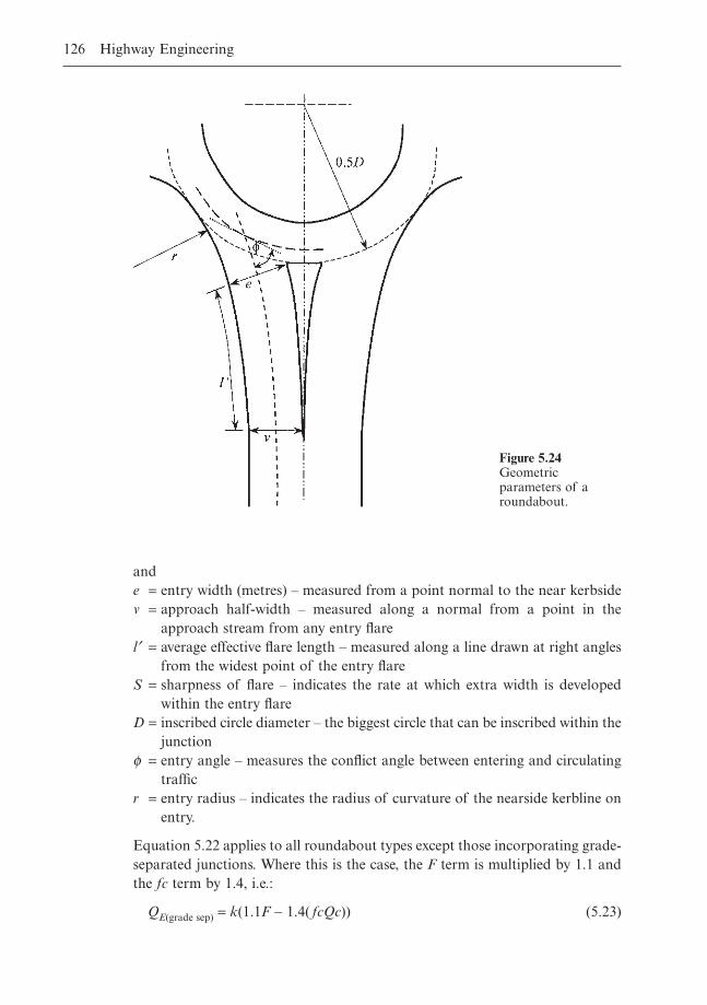
126 Highway Engineering
ande = entry width (metres) – measured from a point normal to the near kerbsidev = approach half-width – measured along a normal from a point in the
approach stream from any entry flarel¢ = average effective flare length – measured along a line drawn at right angles
from the widest point of the entry flareS = sharpness of flare – indicates the rate at which extra width is developed
within the entry flareD = inscribed circle diameter – the biggest circle that can be inscribed within the
junctionf = entry angle – measures the conflict angle between entering and circulating
trafficr = entry radius – indicates the radius of curvature of the nearside kerbline on
entry.
Equation 5.22 applies to all roundabout types except those incorporating grade-separated junctions. Where this is the case, the F term is multiplied by 1.1 andthe fc term by 1.4, i.e.:
QE(grade sep) = k(1.1F - 1.4( fcQc)) (5.23)
Figure 5.24Geometricparameters of aroundabout.
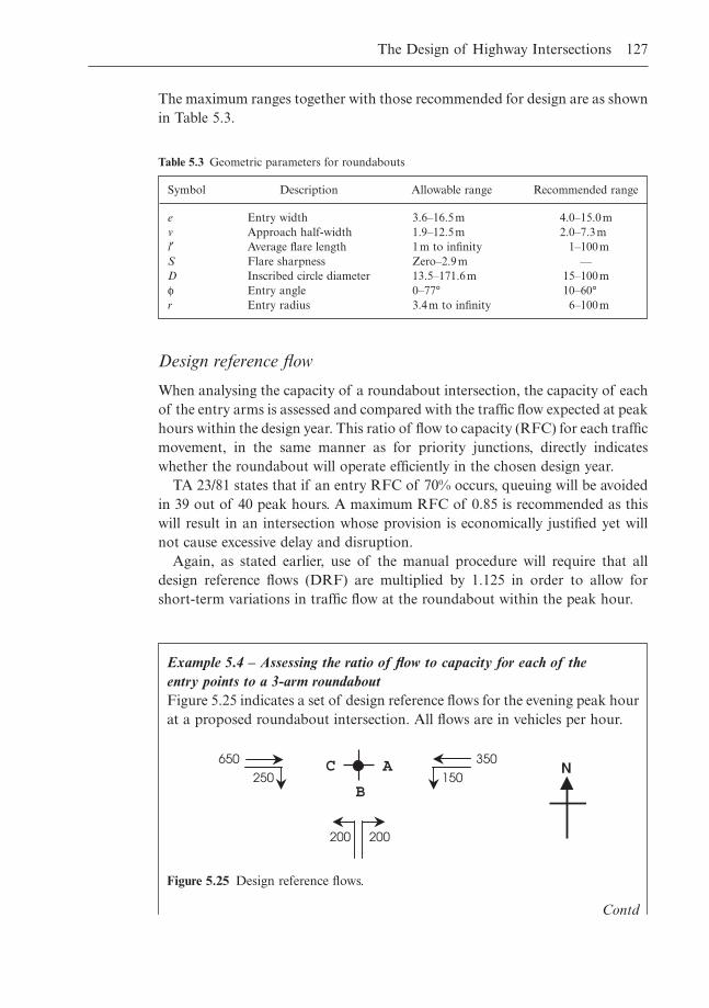
The maximum ranges together with those recommended for design are as shownin Table 5.3.
The Design of Highway Intersections 127
Symbol Description Allowable range Recommended range
e Entry width 3.6–16.5m 4.0–15.0mv Approach half-width 1.9–12.5m 2.0–7.3ml¢ Average flare length 1m to infinity 1–100mS Flare sharpness Zero–2.9m —D Inscribed circle diameter 13.5–171.6m 15–100mf Entry angle 0–77° 10–60°r Entry radius 3.4m to infinity 6–100m
Table 5.3 Geometric parameters for roundabouts
Example 5.4 – Assessing the ratio of flow to capacity for each of the entry points to a 3-arm roundaboutFigure 5.25 indicates a set of design reference flows for the evening peak hourat a proposed roundabout intersection. All flows are in vehicles per hour.
250
650 350
150
200200
AC N
B
Design reference flow
When analysing the capacity of a roundabout intersection, the capacity of eachof the entry arms is assessed and compared with the traffic flow expected at peakhours within the design year. This ratio of flow to capacity (RFC) for each trafficmovement, in the same manner as for priority junctions, directly indicateswhether the roundabout will operate efficiently in the chosen design year.
TA 23/81 states that if an entry RFC of 70% occurs, queuing will be avoidedin 39 out of 40 peak hours. A maximum RFC of 0.85 is recommended as thiswill result in an intersection whose provision is economically justified yet willnot cause excessive delay and disruption.
Again, as stated earlier, use of the manual procedure will require that alldesign reference flows (DRF) are multiplied by 1.125 in order to allow for short-term variations in traffic flow at the roundabout within the peak hour.
Figure 5.25 Design reference flows.
Contd
Values of entry and circulating flows
In order to estimate the circulating flow and thus the entry capacity of eachentry movement using the manual procedure, the entry flow values from Fig. 5.25 are multiplied by a factor of 1.125. The derived flows are then multiplied by 1.1 in order to convert the vehicles to passenger car units (pcu)(Table 5.4).
128 Highway Engineering
Example 5.4 Contd
Estimate the ratio of flow to capacity for each entry point. A heavy goodsvehicle content of 10% is assumed.
The following are the geometric parameters assumed for each entry armat the junction:
e = 7.5mv = 4m (east and west arms), 3.65m (south arm)l¢ = 10mD = 28mf = 30°r = 10m
Thereforek = 0.951S = 0.56 (east and west arms), 0.62 (south arm)X2 = 5.65 (east and west arms), 5.37 (south arm)F = 1712 (east and west arms), 1629 (south arm)M = 0.0408tD = 1.48fc = 0.662 (east and west arms), 0.645 (south arm)
For east arm (Arm A):QE = k(F - fcQc)
= 0.9511(1712 - 0.6622Qc)= 1629 - 0.63Qc
For south arm (Arm B):QE = k(F - fcQc)
= 0.951(1629 - 0.65Qc)= 1549 - 0.614Qc
For west arm (Arm C):QE = k(F - fcQc)
= 0.9511(1712 - 0.662Qc)= 1629 - 0.63Qc
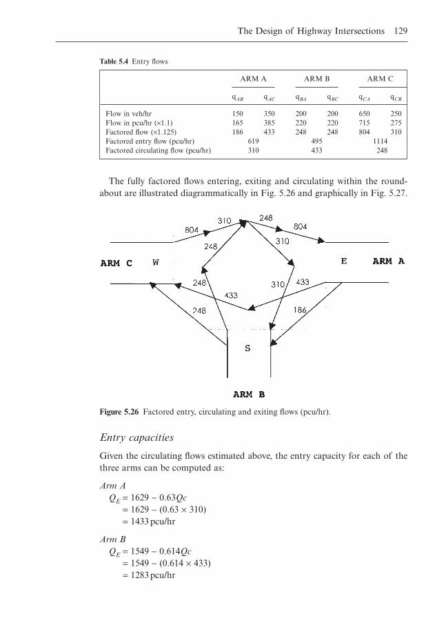
The fully factored flows entering, exiting and circulating within the round-about are illustrated diagrammatically in Fig. 5.26 and graphically in Fig. 5.27.
The Design of Highway Intersections 129
ARM A ARM B ARM C
qAB qAC qBA qBC qCA qCB
Flow in veh/hr 150 350 200 200 650 250Flow in pcu/hr (¥1.1) 165 385 220 220 715 275Factored flow (¥1.125) 186 433 248 248 804 310Factored entry flow (pcu/hr) 619 495 1114Factored circulating flow (pcu/hr) 310 433 248
Table 5.4 Entry flows
Figure 5.26 Factored entry, circulating and exiting flows (pcu/hr).
Entry capacities
Given the circulating flows estimated above, the entry capacity for each of thethree arms can be computed as:
Arm AQE = 1629 - 0.63Qc
= 1629 - (0.63 ¥ 310)= 1433pcu/hr
Arm BQE = 1549 - 0.614Qc
= 1549 - (0.614 ¥ 433)= 1283pcu/hr
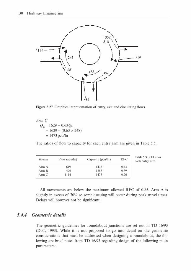
Arm CQE = 1629 - 0.63Qc
= 1629 - (0.63 ¥ 248)= 1473pcu/hr
The ratios of flow to capacity for each entry arm are given in Table 5.5.
130 Highway Engineering
Figure 5.27 Graphical representation of entry, exit and circulating flows.
Stream Flow (pcu/hr) Capacity (pcu/hr) RFC
Arm A 619 1433 0.43Arm B 496 1283 0.39Arm C 1114 1473 0.76
Table 5.5 RFCs foreach entry arm
All movements are below the maximum allowed RFC of 0.85. Arm A isslightly in excess of 70% so some queuing will occur during peak travel times.Delays will however not be significant.
5.4.4 Geometric details
The geometric guidelines for roundabout junctions are set out in TD 16/93(DoT, 1993). While it is not proposed to go into detail on the geometric considerations that must be addressed when designing a roundabout, the fol-lowing are brief notes from TD 16/93 regarding design of the following mainparameters:
� Entry width� Entry angle� Entry radius� Entry deflection� Inscribed circle diameter (ICD)� Circulatory carriageway� Main central island.
Entry width
TD16/93 states that it is good practice to add at least an extra lane to the laneson the entry approach. (This has been done at all entry arms in the aboveexample. In all cases one lane has been widened to two at the entry point.)
Entry angle
It is recommended that the entry angle should be between 10 and 60°. (In theabove example, an entry angle of 30º was used at all entry points.)
Entry radius
The absolute minimum radius should be 6m and, in order to cater for heavygoods vehicles, it should preferably not be less than 10m.
Entry deflection
This is one of the main determinants of safety on a roundabout, indicating thedeflection to the left imposed on all entering vehicles. For each entry arm, thetightest radius of the entry path curvature, measured over a distance of at least20–25m, should not exceed 100m.
Inscribed circle diameter (ICD)
In order to accommodate the turning movement of a standard 15.5m long arti-culated vehicle, the inscribed circle diameter must be at least 28m. The ICD inthe above example is exactly 28m.
Circulatory carriageway
The width of the circulatory should not exceed 15m and should lie between 1.0 and 1.2 times the maximum entry width. The chosen design sets the circulatory carriageway at 9m, approximately 1.2 times the maximum entrywidth value (7.6m).
The Design of Highway Intersections 131
Main central island
The main central island will have a radius of 2m, the maximum allowable foran ICD of 28m, again to allow the safe movement through the junction of largearticulated vehicles. In order to limit the circulatory carriageway, therefore, alow profile subsidiary central island should be provided, extending the radius ofthe central island out to a total of 5m. The subsidiary island provides deflec-tion for standard vehicles while allowing overrun by the rear wheels of articu-lated vehicles.
5.5 Basics of traffic signal control: optimisation and delays
5.5.1 Introduction
Traffic signals work on the basis of allocating separate time periods to conflict-ing traffic movements at a highway intersection so that the available carriage-way space is utilised as efficiently and safely as possible. Priority can be variedwith time through the cycle of the signals. Within urban areas in particular, insituations where a road has a number of intersections along its entire length,signal linking can be used as a method for allowing almost continuous pro-gression of traffic through the route.
In the UK the decision to install traffic lights at a given junction is arrived atthrough assessing in economic terms the reduction in delay resulting from ittogether with the forecasted improvement in accident characteristics and placingthese against the computed capital and operating costs. In the UK the usualsequence for traffic signals is red, red/amber, green and amber. In Ireland, thesequence is red, green and amber.
The installation of traffic signals is justified by the need to:
� Reduce delay to motorists and pedestrians moving through the junction� Reduce accidents at the junction� Improve the control of traffic flow into and through the junction in particu-
lar and the area in general, thereby minimising journey times� Impose certain chosen traffic management policies.
Traffic signals can however have certain disadvantages:
� They must undergo frequent maintenance along with frequent monitoringto ensure their maximum effectiveness
� There can be inefficiencies during off-peak times leading to increases in delayand disruption during these periods
� Increases in rear-end collisions can result� Signal breakdown due to mechanical/electrical failure can cause serious
interruption in traffic flow.
132 Highway Engineering
As with priority junctions and roundabouts, the basis of design in this instanceis the ratio of demand to capacity for each flow path. In addition, however, thesetting of the traffic signal in question is also a relevant parameter. The capac-ity of a given flow path is expressed as its saturation flow, defined as themaximum traffic flow capable of crossing the stop line assuming 100% greentime. Traffic signals will normally operate on the basis of a fixed-time sequence,though vehicle actuated signals can also be installed. The fixed-time sequencemay be programmed to vary depending on the time of day. Typically, a sepa-rate programme may operate for the morning and evening peaks, daytime off-peak and late night/early morning conditions.
5.5.2 Phasing at a signalised intersection
Phasing allows conflicting traffic streams to be separated. A phase is charac-terised as a sequence of conditions applied to one or more traffic streams.During one given cycle, all traffic within a phase will receive identical and simul-taneous signal indications.
Take, for example, a crossroads intersection, where north-south traffic willconflict with that travelling from east to west. Since the number of conflicts istwo, this is the number of required phases. With other more complex intersec-tions, more than two phases will be required. A typical example of this is a cross-roads with a high proportion of right-turning traffic on one of the entry roads,with movement necessitating a dedicated phase. A three-phase system is there-fore designed. Because, as will be shown further below, there are time delaysassociated with each phase within a traffic cycle, efficiency and safety dictatethat the number be kept to a minimum.
The control of traffic movement at a signalised junction is often described interms of the sequential steps in which the control at the intersection is varied.This is called stage control, with a stage usually commencing from the start of an amber period and ending at the start of the following stage. Stages within a traffic cycle are arranged in a predetermined sequence. Figures 5.28 and 5.29 illustrate, respectively, typical two-phase and three-phase signalisedintersections.
5.5.3 Saturation flow
The capacity for each approach to an intersection can be estimated by summingthe saturation flows of the individual lanes within each of the pathways. Themain parameters relevant to the estimation of capacity for each approach are:
� Number, width and location of lanesThe overall capacity of an approach road is equal to the sum of the satura-tion flows for all lanes within it. It is assumed that the average lane width
The Design of Highway Intersections 133
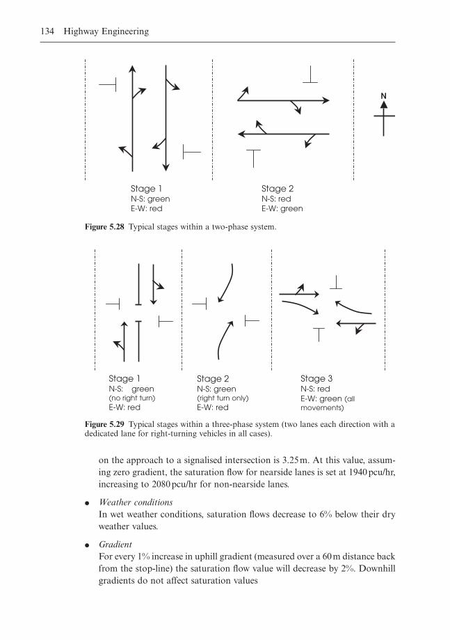
on the approach to a signalised intersection is 3.25m. At this value, assum-ing zero gradient, the saturation flow for nearside lanes is set at 1940pcu/hr,increasing to 2080pcu/hr for non-nearside lanes.
� Weather conditionsIn wet weather conditions, saturation flows decrease to 6% below their dryweather values.
� GradientFor every 1% increase in uphill gradient (measured over a 60m distance backfrom the stop-line) the saturation flow value will decrease by 2%. Downhillgradients do not affect saturation values
134 Highway Engineering
Stage 1N-S: green E-W: red
Stage 2N-S: red E-W: green
N
Figure 5.28 Typical stages within a two-phase system.
Stage 1 N-S: green (no right turn) E-W: red
Stage 2N-S: green (right turn only) E-W: red
Stage 3N-S: red E-W: green (all movements)
Figure 5.29 Typical stages within a three-phase system (two lanes each direction with adedicated lane for right-turning vehicles in all cases).
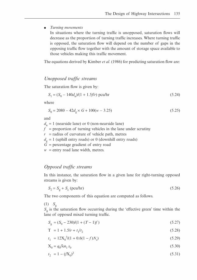
� Turning movementsIn situations where the turning traffic is unopposed, saturation flows willdecrease as the proportion of turning traffic increases. Where turning trafficis opposed, the saturation flow will depend on the number of gaps in theopposing traffic flow together with the amount of storage space available tothose vehicles making this traffic movement.
The equations derived by Kimber et al. (1986) for predicting saturation flow are:
Unopposed traffic streams
The saturation flow is given by:
S1 = (S0 - 140dn)/(1 + 1.5f/r) pcu/hr (5.24)
where
S0 = 2080 - 42dg ¥ G + 100(w - 3.25) (5.25)
anddn = 1 (nearside lane) or 0 (non-nearside lane)f = proportion of turning vehicles in the lane under scrutinyr = radius of curvature of vehicle path, metresdg = 1 (uphill entry roads) or 0 (downhill entry roads)G = percentage gradient of entry roadw = entry road lane width, metres.
Opposed traffic streams
In this instance, the saturation flow in a given lane for right-turning opposedstreams is given by:
S2 = Sg + Sc (pcu/hr) (5.26)
The two components of this equation are computed as follows.
(1) SgSg is the saturation flow occurring during the ‘effective green’ time within thelane of opposed mixed turning traffic.
Sg = (S0 - 230)/(1 + (T - 1)f ) (5.27)
T = 1 + 1.5/r + t1/t2 (5.28)
t1 = 12X02/(1 + 0.6(1 - f )Ns) (5.29)
X0 = q0/ln1 s0 (5.30)
t2 = 1 - (fX0)2 (5.31)
The Design of Highway Intersections 135
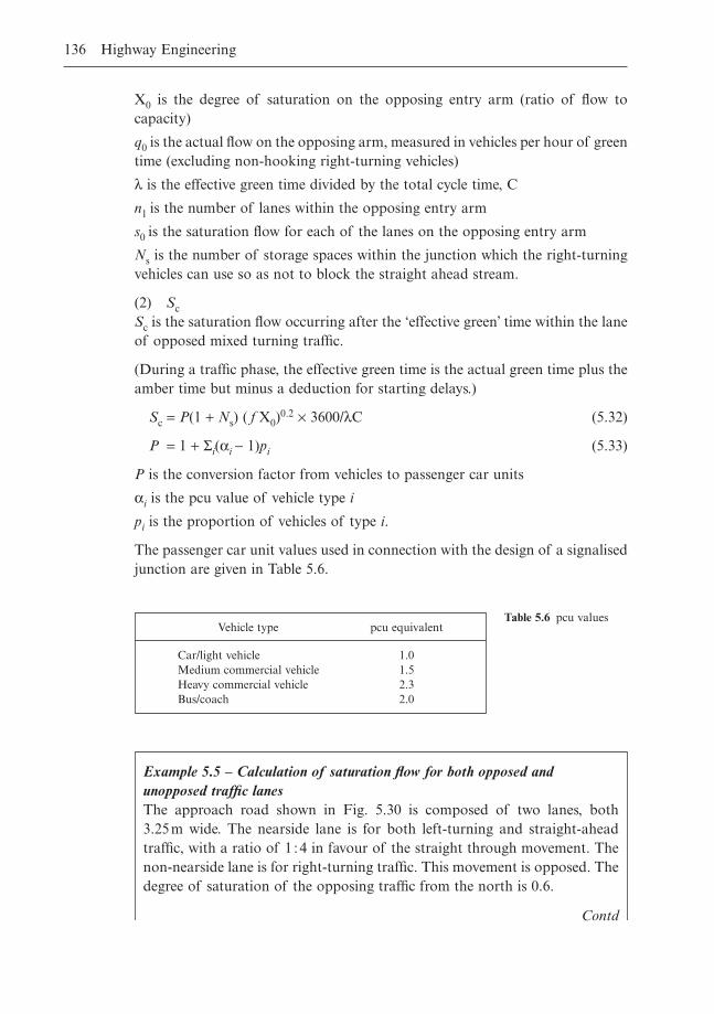
X0 is the degree of saturation on the opposing entry arm (ratio of flow to capacity)
q0 is the actual flow on the opposing arm, measured in vehicles per hour of greentime (excluding non-hooking right-turning vehicles)
l is the effective green time divided by the total cycle time, C
n1 is the number of lanes within the opposing entry arm
s0 is the saturation flow for each of the lanes on the opposing entry arm
Ns is the number of storage spaces within the junction which the right-turningvehicles can use so as not to block the straight ahead stream.
(2) ScSc is the saturation flow occurring after the ‘effective green’ time within the laneof opposed mixed turning traffic.
(During a traffic phase, the effective green time is the actual green time plus theamber time but minus a deduction for starting delays.)
Sc = P(1 + Ns) ( f X0)0.2 ¥ 3600/lC (5.32)
P = 1 + Si(ai - 1)pi (5.33)
P is the conversion factor from vehicles to passenger car units
ai is the pcu value of vehicle type i
pi is the proportion of vehicles of type i.
The passenger car unit values used in connection with the design of a signalisedjunction are given in Table 5.6.
136 Highway Engineering
Vehicle type pcu equivalent
Car/light vehicle 1.0Medium commercial vehicle 1.5Heavy commercial vehicle 2.3Bus/coach 2.0
Table 5.6 pcu values
Example 5.5 – Calculation of saturation flow for both opposed andunopposed traffic lanesThe approach road shown in Fig. 5.30 is composed of two lanes, both 3.25m wide. The nearside lane is for both left-turning and straight-aheadtraffic, with a ratio of 1 :4 in favour of the straight through movement. Thenon-nearside lane is for right-turning traffic. This movement is opposed. Thedegree of saturation of the opposing traffic from the north is 0.6.
Contd
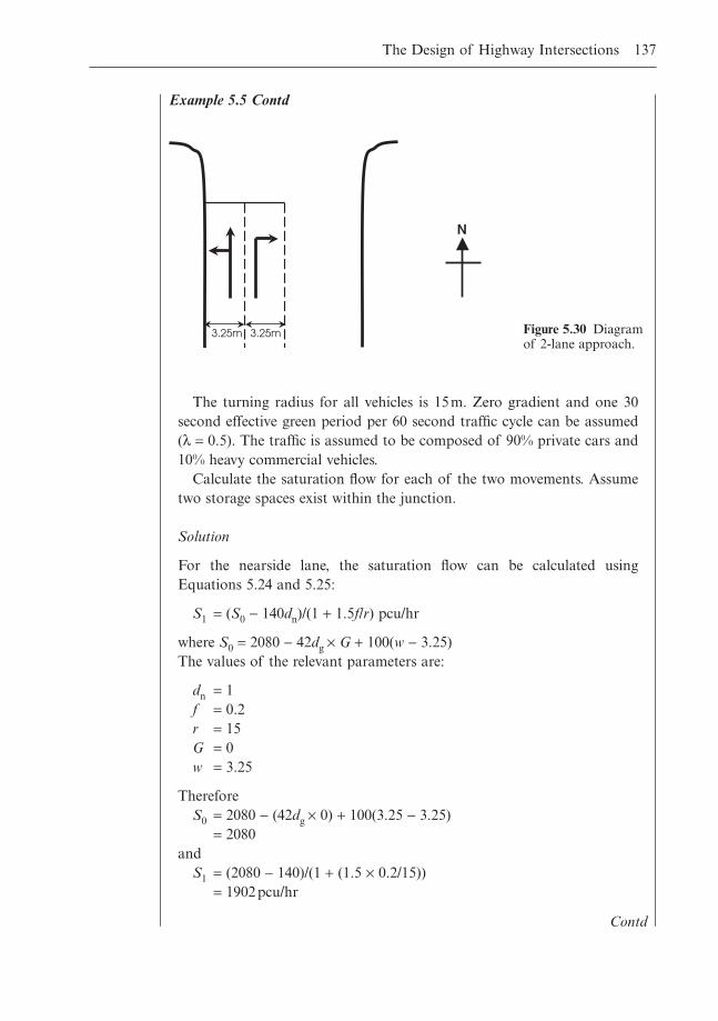
The Design of Highway Intersections 137
Example 5.5 Contd
N
3.25m 3.25m Figure 5.30 Diagramof 2-lane approach.
The turning radius for all vehicles is 15m. Zero gradient and one 30second effective green period per 60 second traffic cycle can be assumed(l = 0.5). The traffic is assumed to be composed of 90% private cars and10% heavy commercial vehicles.
Calculate the saturation flow for each of the two movements. Assumetwo storage spaces exist within the junction.
Solution
For the nearside lane, the saturation flow can be calculated using Equations 5.24 and 5.25:
S1 = (S0 - 140dn)/(1 + 1.5f/r) pcu/hr
where S0 = 2080 - 42dg ¥ G + 100(w - 3.25)The values of the relevant parameters are:
dn = 1f = 0.2r = 15G = 0w = 3.25
ThereforeS0 = 2080 - (42dg ¥ 0) + 100(3.25 - 3.25)
= 2080and
S1 = (2080 - 140)/(1 + (1.5 ¥ 0.2/15))= 1902pcu/hr
Contd
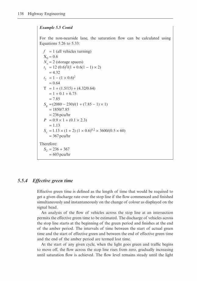
5.5.4 Effective green time
Effective green time is defined as the length of time that would be required toget a given discharge rate over the stop line if the flow commenced and finishedsimultaneously and instantaneously on the change of colour as displayed on thesignal head.
An analysis of the flow of vehicles across the stop line at an intersectionpermits the effective green time to be estimated. The discharge of vehicles acrossthe stop line starts at the beginning of the green period and finishes at the endof the amber period. The intervals of time between the start of actual greentime and the start of effective green and between the end of effective green timeand the end of the amber period are termed lost time.
At the start of any given cycle, when the light goes green and traffic beginsto move off, the flow across the stop line rises from zero, gradually increasinguntil saturation flow is achieved. The flow level remains steady until the light
138 Highway Engineering
Example 5.5 Contd
For the non-nearside lane, the saturation flow can be calculated using Equations 5.26 to 5.33:
f = 1 (all vehicles turning)X0 = 0.6Ns = 2 (storage spaces)t1 = 12 (0.6)2/(1 + 0.6(1 - 1) ¥ 2)
= 4.32t2 = 1 - (1 ¥ 0.6)2
= 0.64T = 1 + (1.5/15) + (4.32/0.64)
= 1 + 0.1 + 6.75= 7.85
Sg = (2080 - 230)/(1 + (7.85 - 1) ¥ 1)= 1850/7.85= 236pcu/hr
P = 0.9 ¥ 1 + (0.1 ¥ 2.3)= 1.13
Sc = 1.13 ¥ (1 + 2) (1 ¥ 0.6)0.2 ¥ 3600/(0.5 ¥ 60)= 367pcu/hr
Therefore:S2 = 236 + 367
= 603pcu/hr
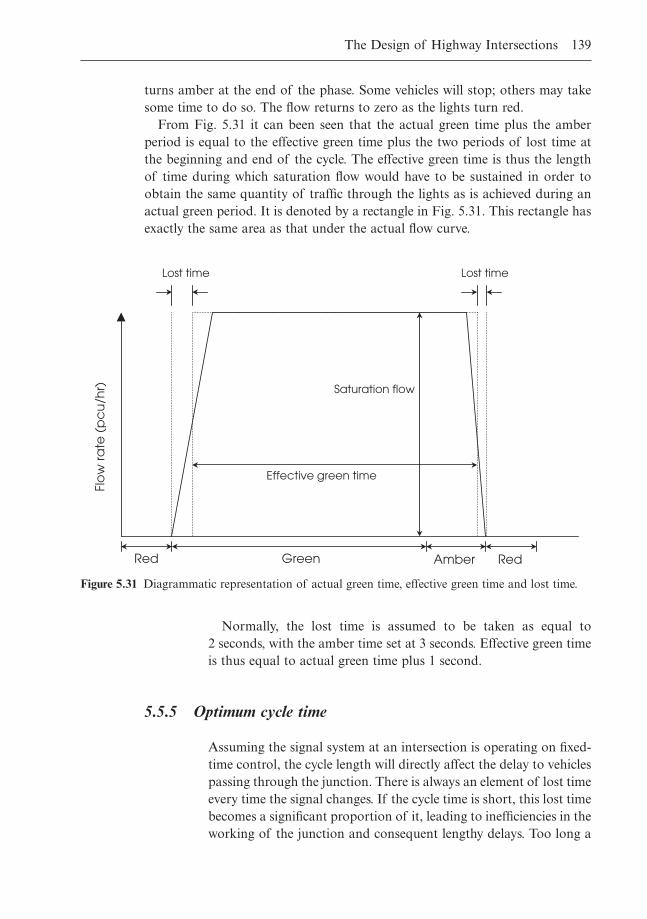
turns amber at the end of the phase. Some vehicles will stop; others may takesome time to do so. The flow returns to zero as the lights turn red.
From Fig. 5.31 it can been seen that the actual green time plus the amberperiod is equal to the effective green time plus the two periods of lost time atthe beginning and end of the cycle. The effective green time is thus the lengthof time during which saturation flow would have to be sustained in order toobtain the same quantity of traffic through the lights as is achieved during anactual green period. It is denoted by a rectangle in Fig. 5.31. This rectangle hasexactly the same area as that under the actual flow curve.
The Design of Highway Intersections 139
Green Amber Red Red
Flo
w ra
te (
pc
u/h
r)
Lost time Lost time
Effective green time
Saturation flow
Figure 5.31 Diagrammatic representation of actual green time, effective green time and lost time.
Normally, the lost time is assumed to be taken as equal to 2 seconds, with the amber time set at 3 seconds. Effective green timeis thus equal to actual green time plus 1 second.
5.5.5 Optimum cycle time
Assuming the signal system at an intersection is operating on fixed-time control, the cycle length will directly affect the delay to vehiclespassing through the junction. There is always an element of lost timeevery time the signal changes. If the cycle time is short, this lost timebecomes a significant proportion of it, leading to inefficiencies in theworking of the junction and consequent lengthy delays. Too long a
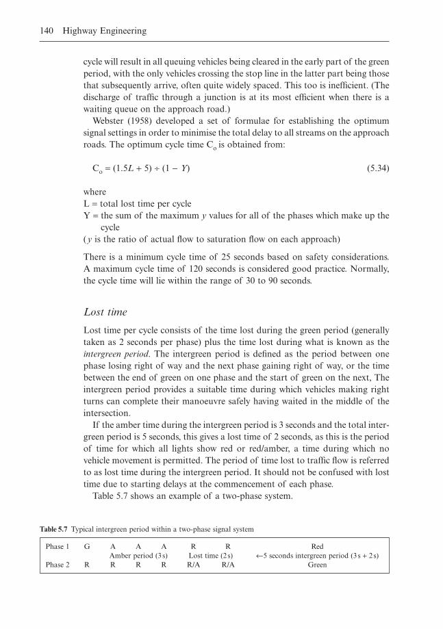
cycle will result in all queuing vehicles being cleared in the early part of the greenperiod, with the only vehicles crossing the stop line in the latter part being thosethat subsequently arrive, often quite widely spaced. This too is inefficient. (Thedischarge of traffic through a junction is at its most efficient when there is awaiting queue on the approach road.)
Webster (1958) developed a set of formulae for establishing the optimumsignal settings in order to minimise the total delay to all streams on the approachroads. The optimum cycle time Co is obtained from:
Co = (1.5L + 5) ∏ (1 - Y) (5.34)
whereL = total lost time per cycleY = the sum of the maximum y values for all of the phases which make up the
cycle(y is the ratio of actual flow to saturation flow on each approach)
There is a minimum cycle time of 25 seconds based on safety considerations.A maximum cycle time of 120 seconds is considered good practice. Normally,the cycle time will lie within the range of 30 to 90 seconds.
Lost time
Lost time per cycle consists of the time lost during the green period (generallytaken as 2 seconds per phase) plus the time lost during what is known as theintergreen period. The intergreen period is defined as the period between onephase losing right of way and the next phase gaining right of way, or the timebetween the end of green on one phase and the start of green on the next, Theintergreen period provides a suitable time during which vehicles making rightturns can complete their manoeuvre safely having waited in the middle of theintersection.
If the amber time during the intergreen period is 3 seconds and the total inter-green period is 5 seconds, this gives a lost time of 2 seconds, as this is the periodof time for which all lights show red or red/amber, a time during which novehicle movement is permitted. The period of time lost to traffic flow is referredto as lost time during the intergreen period. It should not be confused with losttime due to starting delays at the commencement of each phase.
Table 5.7 shows an example of a two-phase system.
140 Highway Engineering
Phase 1 G A A A R R RedAmber period (3 s) Lost time (2 s) ¨5 seconds intergreen period (3 s + 2s)
Phase 2 R R R R R/A R/A Green
Table 5.7 Typical intergreen period within a two-phase signal system
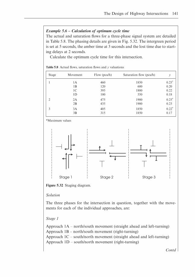
The Design of Highway Intersections 141
Example 5.6 – Calculation of optimum cycle timeThe actual and saturation flows for a three-phase signal system are detailedin Table 5.8. The phasing details are given in Fig. 5.32. The intergreen periodis set at 5 seconds, the amber time at 3 seconds and the lost time due to start-ing delays at 2 seconds.
Calculate the optimum cycle time for this intersection.
Stage Movement Flow (pcu/h) Saturation flow (pcu/h) y
1 1A 460 1850 0.25*
1B 120 600 0.201C 395 1800 0.221D 100 550 0.18
2 2A 475 1900 0.25*
2B 435 1900 0.23
3 3A 405 1850 0.22*
3B 315 1850 0.17
Table 5.8 Actual flows, saturation flows and y valuations
Stage 1 Stage 2 Stage 3
Figure 5.32 Staging diagram.
Solution
The three phases for the intersection in question, together with the move-ments for each of the individual approaches, are:
Stage 1
Approach 1A – north/south movement (straight ahead and left-turning)Approach 1B – north/south movement (right-turning)Approach 1C – south/north movement (straight ahead and left-turning)Approach 1D – south/north movement (right-turning)
Contd
*Maximum values
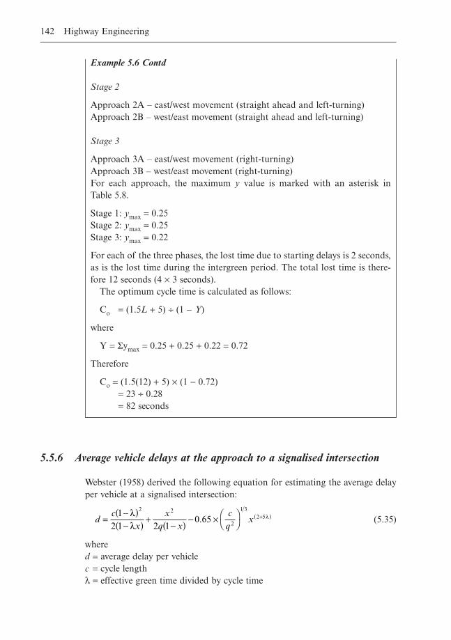
5.5.6 Average vehicle delays at the approach to a signalised intersection
Webster (1958) derived the following equation for estimating the average delayper vehicle at a signalised intersection:
(5.35)
whered = average delay per vehiclec = cycle lengthl = effective green time divided by cycle time
dc
xx
q xc
qx=
-( )-( ) +
-( ) - ¥ ÊË
ˆ¯
+( )12 1 2 1
0 652 2
2
1 32 5l
ll.
142 Highway Engineering
Example 5.6 Contd
Stage 2
Approach 2A – east/west movement (straight ahead and left-turning)Approach 2B – west/east movement (straight ahead and left-turning)
Stage 3
Approach 3A – east/west movement (right-turning)Approach 3B – west/east movement (right-turning)For each approach, the maximum y value is marked with an asterisk in Table 5.8.
Stage 1: ymax = 0.25Stage 2: ymax = 0.25Stage 3: ymax = 0.22
For each of the three phases, the lost time due to starting delays is 2 seconds,as is the lost time during the intergreen period. The total lost time is there-fore 12 seconds (4 ¥ 3 seconds).
The optimum cycle time is calculated as follows:
Co = (1.5L + 5) ∏ (1 - Y)
where
Y = Symax = 0.25 + 0.25 + 0.22 = 0.72
Therefore
Co = (1.5(12) + 5) ¥ (1 - 0.72)= 23 ∏ 0.28= 82 seconds
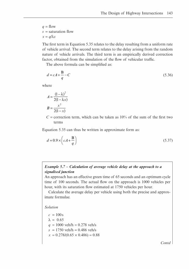
q = flows = saturation flowx = q/ls
The first term in Equation 5.35 relates to the delay resulting from a uniform rateof vehicle arrival. The second term relates to the delay arising from the randomnature of vehicle arrivals. The third term is an empirically derived correctionfactor, obtained from the simulation of the flow of vehicular traffic.
The above formula can be simplified as:
(5.36)
where
C = correction term, which can be taken as 10% of the sum of the first twoterms
Equation 5.35 can thus be written in approximate form as:
(5.37)d cAq
= ¥ +ÊË
ˆ¯0 9.
B
Ax
Bx
x
=-( )-( )
=-( )
12 1
2 1
2
2
ll
d cAq
C= + -B
The Design of Highway Intersections 143
Example 5.7 – Calculation of average vehicle delay at the approach to asignalised junctionAn approach has an effective green time of 65 seconds and an optimum cycletime of 100 seconds. The actual flow on the approach is 1000 vehicles perhour, with its saturation flow estimated at 1750 vehicles per hour.
Calculate the average delay per vehicle using both the precise and approx-imate formulae.
Solution
c = 100sl = 0.65q = 1000 veh/h = 0.278 veh/ss = 1750 veh/h = 0.486 veh/sx = 0.278/(0.65 ¥ 0.486) = 0.88
Contd
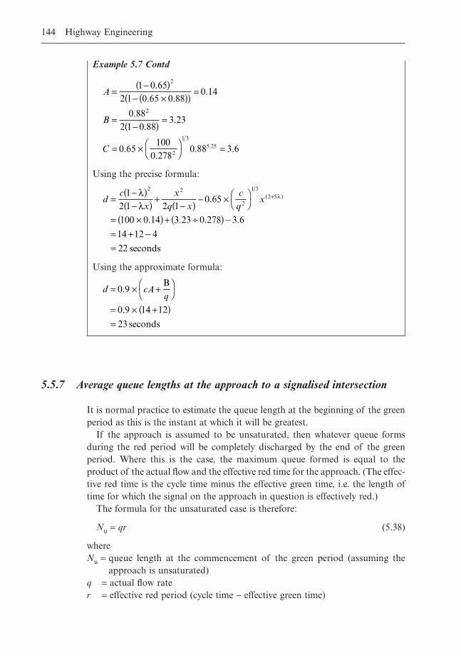
5.5.7 Average queue lengths at the approach to a signalised intersection
It is normal practice to estimate the queue length at the beginning of the greenperiod as this is the instant at which it will be greatest.
If the approach is assumed to be unsaturated, then whatever queue formsduring the red period will be completely discharged by the end of the greenperiod. Where this is the case, the maximum queue formed is equal to theproduct of the actual flow and the effective red time for the approach. (The effec-tive red time is the cycle time minus the effective green time, i.e. the length oftime for which the signal on the approach in question is effectively red.)
The formula for the unsaturated case is therefore:
Nu = qr (5.38)
whereNu = queue length at the commencement of the green period (assuming the
approach is unsaturated)q = actual flow rater = effective red period (cycle time - effective green time)
144 Highway Engineering
Example 5.7 Contd
Using the precise formula:
Using the approximate formula:
d cAq
= ¥ +ÊË
ˆ¯
= ¥ +( )=
0 9
0 9 14 12
23
.
.
B
seconds
dc
xx
q xc
qx=
-( )-( ) +
-( ) - ¥ ÊË
ˆ¯
= ¥( ) + ∏( ) -= + -=
+( )12 1 2 1
0 65
100 0 14 3 23 0 278 3 6
14 12 4
22
2 2
2
1 32 5l
ll.
. . . .
seconds
A
B
C
=-( )
- ¥( )( ) =
=-( ) =
= ¥ ÊË
ˆ¯ =
1 0 652 1 0 65 0 88
0 14
0 882 1 0 88
3 23
0 65100
0 2780 88 3 6
2
2
2
1 35 25
.. .
.
..
.
..
. ..
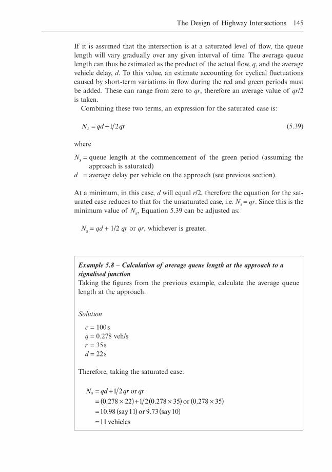
If it is assumed that the intersection is at a saturated level of flow, the queuelength will vary gradually over any given interval of time. The average queuelength can thus be estimated as the product of the actual flow, q, and the averagevehicle delay, d. To this value, an estimate accounting for cyclical fluctuationscaused by short-term variations in flow during the red and green periods mustbe added. These can range from zero to qr, therefore an average value of qr/2is taken.
Combining these two terms, an expression for the saturated case is:
(5.39)
where
Ns = queue length at the commencement of the green period (assuming theapproach is saturated)
d = average delay per vehicle on the approach (see previous section).
At a minimum, in this case, d will equal r/2, therefore the equation for the sat-urated case reduces to that for the unsaturated case, i.e. Ns = qr. Since this is theminimum value of Ns, Equation 5.39 can be adjusted as:
Ns = qd + 1/2 qr or qr, whichever is greater.
N qd qrs = +1 2
The Design of Highway Intersections 145
Example 5.8 – Calculation of average queue length at the approach to asignalised junctionTaking the figures from the previous example, calculate the average queuelength at the approach.
Solution
c = 100sq = 0.278 veh/sr = 35sd = 22s
Therefore, taking the saturated case:
N qd qr qrs or
or 0.278
say11 or 9.73 say10
vehicles
= += ¥( ) + ¥( ) ¥( )= ( ) ( )=
1 2
0 278 22 1 2 0 278 35 35
10 98
11
. .
.
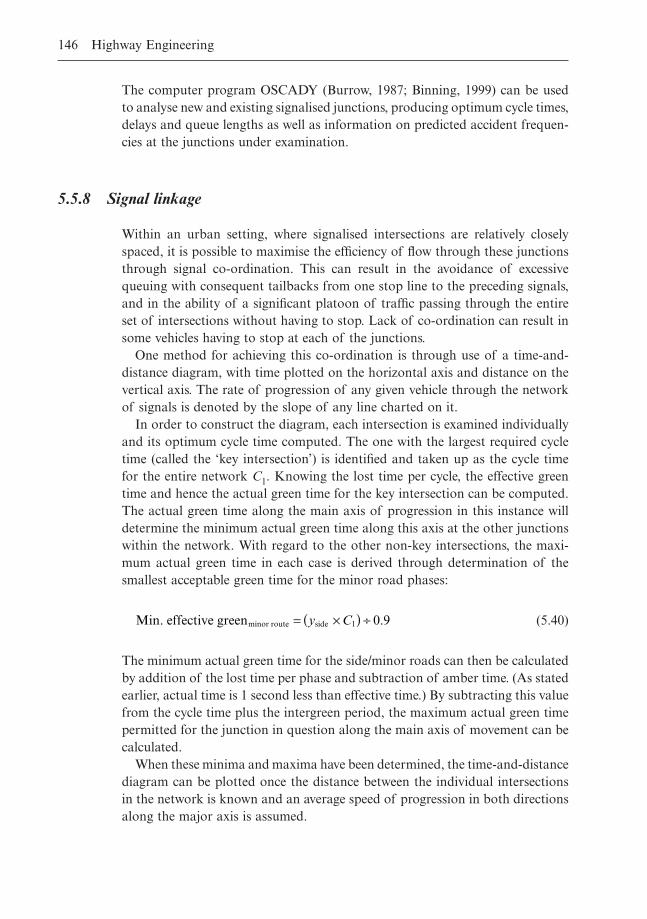
The computer program OSCADY (Burrow, 1987; Binning, 1999) can be usedto analyse new and existing signalised junctions, producing optimum cycle times,delays and queue lengths as well as information on predicted accident frequen-cies at the junctions under examination.
5.5.8 Signal linkage
Within an urban setting, where signalised intersections are relatively closelyspaced, it is possible to maximise the efficiency of flow through these junctionsthrough signal co-ordination. This can result in the avoidance of excessivequeuing with consequent tailbacks from one stop line to the preceding signals,and in the ability of a significant platoon of traffic passing through the entireset of intersections without having to stop. Lack of co-ordination can result insome vehicles having to stop at each of the junctions.
One method for achieving this co-ordination is through use of a time-and-distance diagram, with time plotted on the horizontal axis and distance on the vertical axis. The rate of progression of any given vehicle through the networkof signals is denoted by the slope of any line charted on it.
In order to construct the diagram, each intersection is examined individuallyand its optimum cycle time computed. The one with the largest required cycletime (called the ‘key intersection’) is identified and taken up as the cycle timefor the entire network C1. Knowing the lost time per cycle, the effective greentime and hence the actual green time for the key intersection can be computed.The actual green time along the main axis of progression in this instance willdetermine the minimum actual green time along this axis at the other junctionswithin the network. With regard to the other non-key intersections, the maxi-mum actual green time in each case is derived through determination of thesmallest acceptable green time for the minor road phases:
(5.40)
The minimum actual green time for the side/minor roads can then be calculatedby addition of the lost time per phase and subtraction of amber time. (As statedearlier, actual time is 1 second less than effective time.) By subtracting this valuefrom the cycle time plus the intergreen period, the maximum actual green timepermitted for the junction in question along the main axis of movement can becalculated.
When these minima and maxima have been determined, the time-and-distancediagram can be plotted once the distance between the individual intersectionsin the network is known and an average speed of progression in both directionsalong the major axis is assumed.
Min. effective greenminor route side= ¥( ) ∏y C1 0 9.
146 Highway Engineering
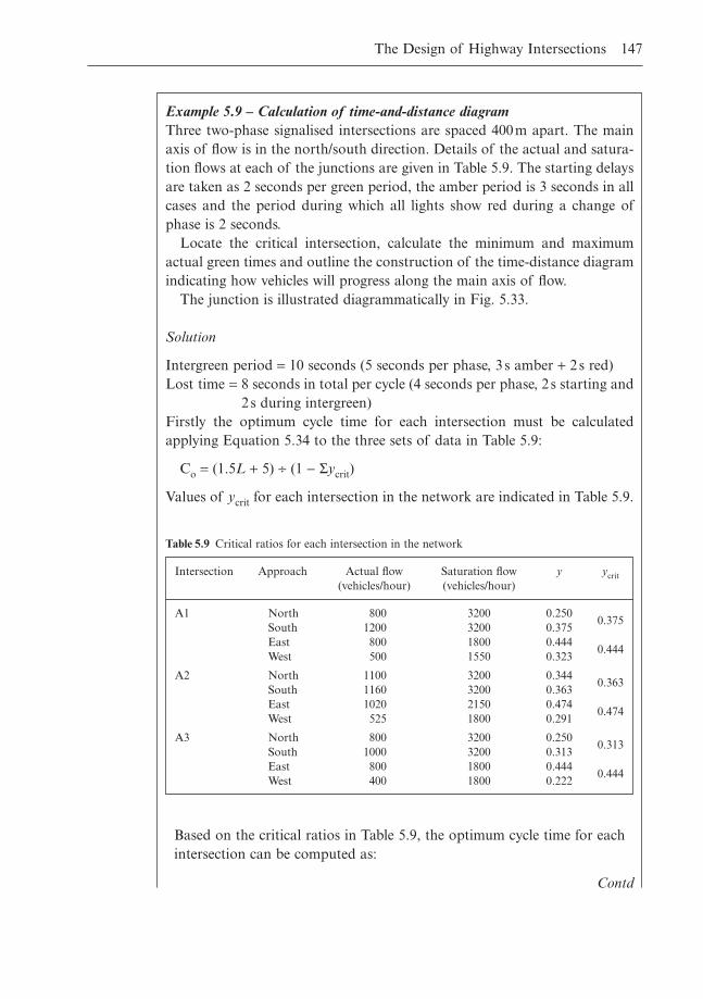
The Design of Highway Intersections 147
Example 5.9 – Calculation of time-and-distance diagramThree two-phase signalised intersections are spaced 400m apart. The mainaxis of flow is in the north/south direction. Details of the actual and satura-tion flows at each of the junctions are given in Table 5.9. The starting delaysare taken as 2 seconds per green period, the amber period is 3 seconds in allcases and the period during which all lights show red during a change ofphase is 2 seconds.
Locate the critical intersection, calculate the minimum and maximumactual green times and outline the construction of the time-distance diagramindicating how vehicles will progress along the main axis of flow.
The junction is illustrated diagrammatically in Fig. 5.33.
Solution
Intergreen period = 10 seconds (5 seconds per phase, 3 s amber + 2s red)Lost time = 8 seconds in total per cycle (4 seconds per phase, 2 s starting and
2s during intergreen)Firstly the optimum cycle time for each intersection must be calculated applying Equation 5.34 to the three sets of data in Table 5.9:
Co = (1.5L + 5) ∏ (1 - Sycrit)
Values of ycrit for each intersection in the network are indicated in Table 5.9.
Intersection Approach Actual flow Saturation flow y ycrit(vehicles/hour) (vehicles/hour)
A1 North 800 3200 0.250South 1200 3200 0.375
0.375
East 800 1800 0.444West 500 1550 0.323
0.444
A2 North 1100 3200 0.344South 1160 3200 0.363
0.363
East 1020 2150 0.474West 525 1800 0.291
0.474
A3 North 800 3200 0.250South 1000 3200 0.313
0.313
East 800 1800 0.444West 400 1800 0.222
0.444
Table 5.9 Critical ratios for each intersection in the network
Based on the critical ratios in Table 5.9, the optimum cycle time for eachintersection can be computed as:
Contd
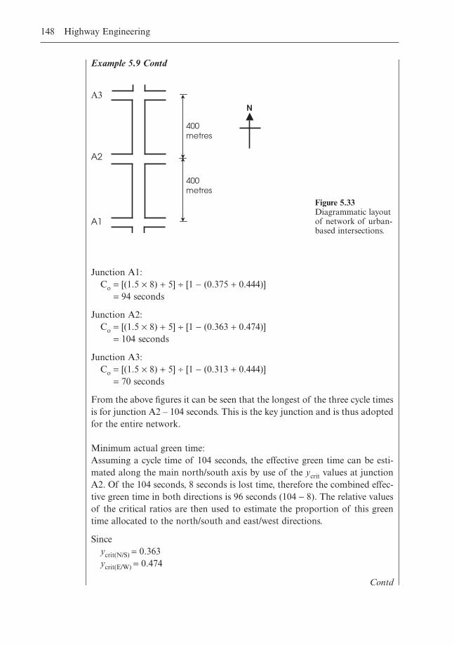
148 Highway Engineering
Example 5.9 Contd
A1
A2
A3
400 metres
400 metres
N
Figure 5.33Diagrammatic layoutof network of urban-based intersections.
Junction A1:Co = [(1.5 ¥ 8) + 5] ∏ [1 - (0.375 + 0.444)]
= 94 seconds
Junction A2:Co = [(1.5 ¥ 8) + 5] ∏ [1 - (0.363 + 0.474)]
= 104 seconds
Junction A3:Co = [(1.5 ¥ 8) + 5] ∏ [1 - (0.313 + 0.444)]
= 70 seconds
From the above figures it can be seen that the longest of the three cycle timesis for junction A2 – 104 seconds. This is the key junction and is thus adoptedfor the entire network.
Minimum actual green time:Assuming a cycle time of 104 seconds, the effective green time can be esti-mated along the main north/south axis by use of the ycrit values at junctionA2. Of the 104 seconds, 8 seconds is lost time, therefore the combined effec-tive green time in both directions is 96 seconds (104 - 8). The relative valuesof the critical ratios are then used to estimate the proportion of this greentime allocated to the north/south and east/west directions.
Sinceycrit(N/S) = 0.363ycrit(E/W) = 0.474
Contd
The Design of Highway Intersections 149
Example 5.9 Contd
Given that starting delays are 2 seconds and the amber time is 3 seconds, theactual green time is equal to the effective green time minus 1 second:
(Minimum actual green time)N/S = 42 - 1= 41 seconds
This figure is adopted as the minimum green time for the remaining two junc-tions within the network (A1 and A3).
Maximum actual green time:The upper limit for actual green time at A1 and A3 is computed by con-sideration of the minimum effective green time required by traffic at thesejunctions along their east/west axis (termed side traffic):
(Minimum effective green time)E/W = (C1 ¥ ycrit(E/W)) ∏ 0.9= (104 ¥ ycrit(E/W)) ∏ 0.9= 116 ¥ ycrit(E/W)
For both A1 and A3:
ycrit(E/W) = 0.444
Therefore
(Minimum effective green time)E/W = 116 ¥ 0.444= 52 seconds
Again, given that starting delays are 2 seconds and the amber time is 3 seconds, the actual green time is equal to the effective green time minus 1 second:
(Minimum actual green time)E/W = 52 - 1 = 51 seconds
The total actual green time for both the north/south and east/west phases is 94 seconds, estimated from the subtraction of the intergreen period (10s) from the total cycle time (104s). Subtracting the minimum actual greentime along the side route from this figure yields the maximum actual green time along the main north/south axis. Therefore, for both A1 and A3intersections:
(Maximum actual green time)N/S = 94 - 51 = 43 seconds
Minimum effective green time
seconds
N S( ) = ¥+
ÈÎÍ
˘˚̇
=
960 363
0 363 0 47442
.. .
Contd
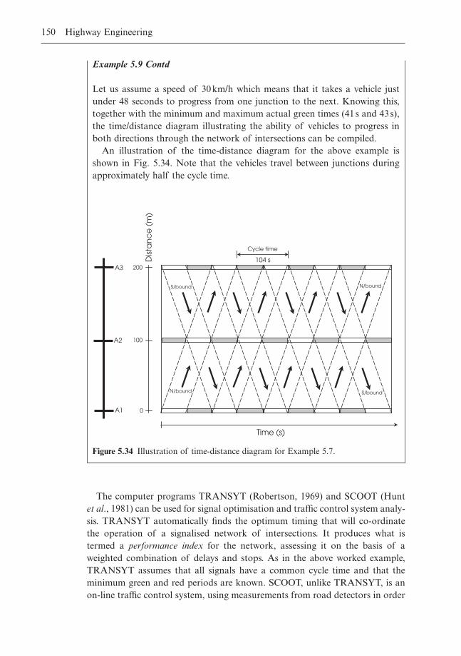
150 Highway Engineering
Example 5.9 Contd
Let us assume a speed of 30km/h which means that it takes a vehicle justunder 48 seconds to progress from one junction to the next. Knowing this,together with the minimum and maximum actual green times (41s and 43s),the time/distance diagram illustrating the ability of vehicles to progress inboth directions through the network of intersections can be compiled.
An illustration of the time-distance diagram for the above example isshown in Fig. 5.34. Note that the vehicles travel between junctions duringapproximately half the cycle time.
104 s
N/bound
N/bound
Dis
tan
ce
(m
)
A3
A2
A1
S/bound
S/bound
100
200
0
Cycle time
Time (s)
Figure 5.34 Illustration of time-distance diagram for Example 5.7.
The computer programs TRANSYT (Robertson, 1969) and SCOOT (Huntet al., 1981) can be used for signal optimisation and traffic control system analy-sis. TRANSYT automatically finds the optimum timing that will co-ordinatethe operation of a signalised network of intersections. It produces what istermed a performance index for the network, assessing it on the basis of aweighted combination of delays and stops. As in the above worked example,TRANSYT assumes that all signals have a common cycle time and that theminimum green and red periods are known. SCOOT, unlike TRANSYT, is anon-line traffic control system, using measurements from road detectors in order
to compile cyclic traffic flow profiles for each junction in the network beingexamined. These profiles are utilised to compute the best possible set of signaltimings for all signals in the network area.
5.6 Concluding remarks
Within the design process for an at-grade intersection, whether it is a priorityjunction, roundabout or signalised junction, the same basic design procedure isemployed. Firstly the traffic data must be collected, indicating the proposedloading on the junction during peak times. Data on the physical characteristicsof the site must also be available, in particular horizontal and vertical align-ments in the vicinity. Design standards may then dictate what type of intersec-tion is employed. The design of the junction itself will be an iterative process,where layouts may be altered based on operating, cost and environmental concerns.
The design of grade separated intersections is not detailed within this text.See O’Flaherty (1997) for details of this intersection type.
5.7 References
Binning, J.C. (1999) OSCADY 4 – User Guide (Application Guide 25). Transport andRoad Research Laboratory, Crowthorne, UK.
Burrow, I.J. (1987) OSCADY – A computer program to model capacities, queues and delaysat isolated traffic signal junctions. TRRL Report RR105. Transport and Road ResearchLaboratory, Crowthorne, UK.
DoT (1981) Junctions and Accesses: Determination of Size of Roundabouts andMajor/Minor Junctions. Departmental Advice Note TA 23/81. Design Manual forRoads and Bridges, Volume 6: Road Geometry. The Stationery Office, London, UK.
DoT (1985) Traffic flows and carriageway width assessments. Departmental StandardTD 20/85. Design Manual for Roads and Bridges, Volume 5: Assessment and Prepara-tion of Road Schemes. The Stationery Office, London, UK.
DoT (1993) The geometric design of roundabouts. Departmental Standard TD 16/93. TheStationery Office, London, UK.
DoT (1995) Geometric Design of Major/Minor Priority Junctions, Departmental Stan-dard TD 42/95. Design Manual for Roads and Bridges, Volume 6: Road Geometry. TheStationery Office, London, UK.
DoT (1996) Traffic Appraisal Manual. Design Manual for Roads and Bridges, Volume 12:Traffic Appraisal of Road Schemes. The Stationery Office, London, UK.
Hunt, P.B., Robertson, D.I. & Bretherton, R.D. (1981) SCOOT – A traffic responsivemethod of coordinating signals. Laboratory Report LR 1014. Transport and RoadResearch Laboratory, Crowthorne, UK.
Kimber, R.M. (1980) The traffic capacity of roundabouts. TRRL Report LR942. Trans-port and Road Research Laboratory, Crowthorne, UK.
The Design of Highway Intersections 151

Kimber, R.M. & Hollis, E.M. (1979) Traffic queues and delays at road junctions. TRRLReport LR909. Transport and Road Research Laboratory, Crowthorne, UK.
Kimber, R.M., McDonald, M. & Hounsell, N.B. (1986) The prediction of saturation flowsfor road junctions controlled by traffic signals. TRRL Research Report 67. Transportand Road Research Laboratory, Crowthorne, UK.
O’Flaherty, C.A. (1997) Transport Planning and Traffic Engineering. Butterworth Heine-mann, Oxford.
Robertson, D.I. (1969) TRANSYT – A traffic network study tool. Laboratory Report LR253. Transport Research Laboratory, Crowthorne, UK.
Semmens, M.C. (1985) PICADY2 – An enhanced programme for modelling traffic capac-ities, queues and delays at major/minor junctions. TRRL Report RR36. Transport andRoad Research Laboratory, Crowthorne, UK.
Webster, F.V. (1958) Traffic signal settings. Road Research Technical Paper No. 39. TheStationery Office, London.
152 Highway Engineering
Chapter 6
Geometric Alignment and Design
6.1 Basic physical elements of a highway
The basic features of a highway are the carriageway itself, expressed in terms ofthe number of lanes used, the central reservation or median strip and the shoul-ders (including verges). Depending on the level of the highway relative to thesurrounding terrain, side-slopes may also be a design issue.
Main carriageway
The chosen carriageway depends on a number of factors, most notably thevolume of traffic using the highway, the quality of service expected from theinstallation and the selected design speed. In most situations a lane width of3.65m is used, making a standard divided or undivided 2-lane carriageway 7.3m wide in total.
Table 6.1 gives a summary of carriageway widths normally used in the UK.These widths are as stated in TD 27/96 (DoT, 1996). Any reduction or increasein these widths is considered a departure from standard. The stated lane widthsshould only be departed from in exceptional circumstances such as where cyclistsneed to be accommodated or where the number of lanes needs to be maximisedfor the amount of land available. In Scotland and Northern Ireland, a total car-riageway width of 6.0m may be used on single carriageway all-purpose roadswhere daily flow in the design year is estimated not to exceed 5000 vehicles.
Central reservation
A median strip or central reservation divides all motorways/dual carriageways.Its main function is to make driving safer for the motorist by limiting locationswhere vehicles can turn right (on dual carriageways), completely separating thetraffic travelling in opposing directions and providing a space where vehicles canrecover their position if for some reason they have unintentionally left the carriageway. In urban settings, a width of 4.5m is recommended for 2/3-lanedual carriageways, with 4.0m recommended for rural highways of this type.While these values should be the first option, a need to minimise land take might
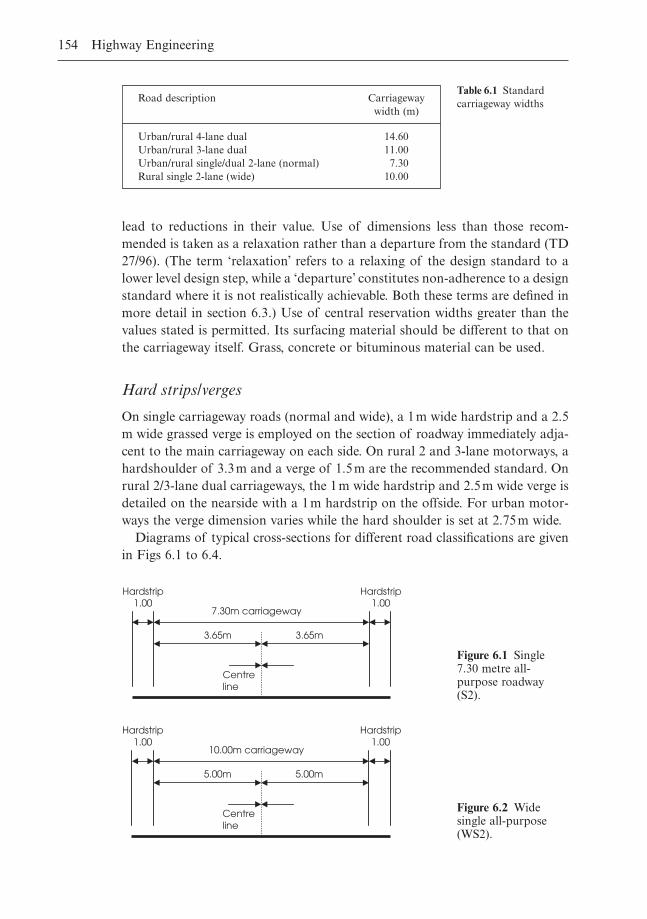
lead to reductions in their value. Use of dimensions less than those recom-mended is taken as a relaxation rather than a departure from the standard (TD27/96). (The term ‘relaxation’ refers to a relaxing of the design standard to alower level design step, while a ‘departure’ constitutes non-adherence to a designstandard where it is not realistically achievable. Both these terms are defined inmore detail in section 6.3.) Use of central reservation widths greater than thevalues stated is permitted. Its surfacing material should be different to that onthe carriageway itself. Grass, concrete or bituminous material can be used.
Hard strips/verges
On single carriageway roads (normal and wide), a 1m wide hardstrip and a 2.5m wide grassed verge is employed on the section of roadway immediately adja-cent to the main carriageway on each side. On rural 2 and 3-lane motorways, ahardshoulder of 3.3m and a verge of 1.5m are the recommended standard. Onrural 2/3-lane dual carriageways, the 1m wide hardstrip and 2.5m wide verge isdetailed on the nearside with a 1m hardstrip on the offside. For urban motor-ways the verge dimension varies while the hard shoulder is set at 2.75m wide.
Diagrams of typical cross-sections for different road classifications are givenin Figs 6.1 to 6.4.
154 Highway Engineering
Road description Carriagewaywidth (m)
Urban/rural 4-lane dual 14.60Urban/rural 3-lane dual 11.00Urban/rural single/dual 2-lane (normal) 7.30Rural single 2-lane (wide) 10.00
Table 6.1 Standardcarriageway widths
Centreline
Hardstrip 1.00
Hardstrip1.00
7.30m carriageway
3.65m 3.65m
Figure 6.1 Single7.30 metre all-purpose roadway(S2).
10.00m carriageway
Centreline
Hardstrip 1.00
Hardstrip1.00
5.00m 5.00m
Figure 6.2 Widesingle all-purpose(WS2).
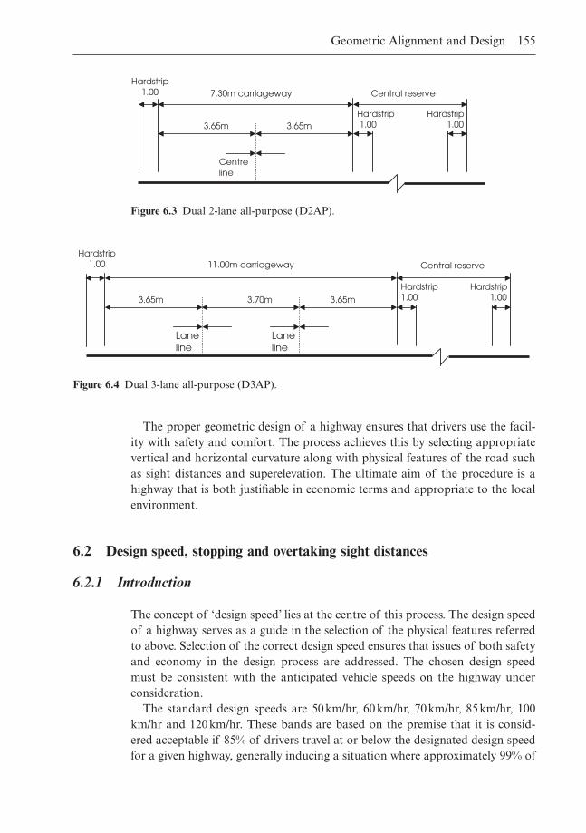
The proper geometric design of a highway ensures that drivers use the facil-ity with safety and comfort. The process achieves this by selecting appropriatevertical and horizontal curvature along with physical features of the road suchas sight distances and superelevation. The ultimate aim of the procedure is ahighway that is both justifiable in economic terms and appropriate to the localenvironment.
6.2 Design speed, stopping and overtaking sight distances
6.2.1 Introduction
The concept of ‘design speed’ lies at the centre of this process. The design speedof a highway serves as a guide in the selection of the physical features referredto above. Selection of the correct design speed ensures that issues of both safetyand economy in the design process are addressed. The chosen design speed must be consistent with the anticipated vehicle speeds on the highway underconsideration.
The standard design speeds are 50km/hr, 60km/hr, 70km/hr, 85km/hr, 100km/hr and 120km/hr. These bands are based on the premise that it is consid-ered acceptable if 85% of drivers travel at or below the designated design speedfor a given highway, generally inducing a situation where approximately 99% of
Geometric Alignment and Design 155
Centre line
7.30m carriageway Central reserveHardstrip
1.00
Hardstrip 1.00
Hardstrip 1.003.65m 3.65m
Figure 6.3 Dual 2-lane all-purpose (D2AP).
Hardstrip 1.00
Central reserve
Hardstrip 1.00
11.00m carriageway
Laneline
Hardstrip 1.00
Lane line
3.70m 3.65m 3.65m
Figure 6.4 Dual 3-lane all-purpose (D3AP).
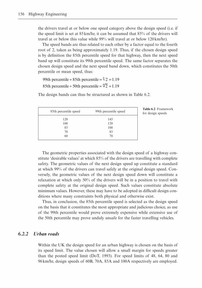
the drivers travel at or below one speed category above the design speed (i.e. ifthe speed limit is set at 85km/hr, it can be assumed that 85% of the drivers willtravel at or below this value while 99% will travel at or below 120km/hr).
The speed bands are thus related to each other by a factor equal to the fourthroot of 2, taken as being approximately 1.19. Thus, if the chosen design speedis by definition the 85th percentile speed for that highway, then the next speedband up will constitute its 99th percentile speed. The same factor separates thechosen design speed and the next speed band down, which constitutes the 50thpercentile or mean speed, thus:
The design bands can thus be structured as shown in Table 6.2.
99 2 1 19
8 0 2 1 19
4
4
th percentile 85th percentile
5th percentile 5 th percentile
∏ = =∏ = =
.
.
156 Highway Engineering
85th percentile speed 99th percentile speed
120 145100 12085 10070 8560 70
Table 6.2 Frameworkfor design speeds
The geometric properties associated with the design speed of a highway con-stitute ‘desirable values’ at which 85% of the drivers are travelling with completesafety. The geometric values of the next design speed up constitute a standardat which 99% of the drivers can travel safely at the original design speed. Con-versely, the geometric values of the next design speed down will constitute arelaxation at which only 50% of the drivers will be in a position to travel withcomplete safety at the original design speed. Such values constitute absoluteminimum values. However, these may have to be adopted in difficult design con-ditions where many constraints both physical and otherwise exist.
Thus, in conclusion, the 85th percentile speed is selected as the design speedon the basis that it constitutes the most appropriate and judicious choice, as useof the 99th percentile would prove extremely expensive while extensive use ofthe 50th percentile may prove unduly unsafe for the faster travelling vehicles.
6.2.2 Urban roads
Within the UK the design speed for an urban highway is chosen on the basis ofits speed limit. The value chosen will allow a small margin for speeds greaterthan the posted speed limit (DoT, 1993). For speed limits of 48, 64, 80 and 96km/hr, design speeds of 60B, 70A, 85A and 100A respectively are employed.
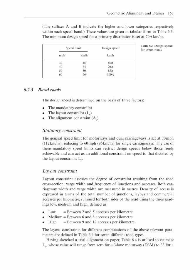
(The suffixes A and B indicate the higher and lower categories respectivelywithin each speed band.) These values are given in tabular form in Table 6.3.The minimum design speed for a primary distributor is set at 70Akm/hr.
Geometric Alignment and Design 157
Speed limit Design speed
mph km/h km/h
30 48 60B40 64 70A50 80 85A60 96 100A
Table 6.3 Design speedsfor urban roads
6.2.3 Rural roads
The design speed is determined on the basis of three factors:
� The mandatory constraint� The layout constraint (Lc)� The alignment constraint (Ac).
Statutory constraint
The general speed limit for motorways and dual carriageways is set at 70mph(112km/hr), reducing to 60mph (96km/hr) for single carriageways. The use ofthese mandatory speed limits can restrict design speeds below those freelyachievable and can act as an additional constraint on speed to that dictated bythe layout constraint Lc.
Layout constraint
Layout constraint assesses the degree of constraint resulting from the roadcross-section, verge width and frequency of junctions and accesses. Both car-riageway width and verge width are measured in metres. Density of access isexpressed in terms of the total number of junctions, laybys and commercialaccesses per kilometre, summed for both sides of the road using the three grad-ings low, medium and high, defined as:
� Low = Between 2 and 5 accesses per kilometre� Medium = Between 6 and 8 accesses per kilometre� High = Between 9 and 12 accesses per kilometre.
The layout constraints for different combinations of the above relevant para-meters are defined in Table 6.4 for seven different road types.
Having sketched a trial alignment on paper, Table 6.4 is utilised to estimateLc, whose value will range from zero for a 3-lane motorway (D3M) to 33 for a
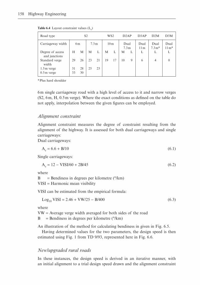
6m single carriageway road with a high level of access to it and narrow verges(S2, 6m, H, 0.5m verge). Where the exact conditions as defined on the table donot apply, interpolation between the given figures can be employed.
Alignment constraint
Alignment constraint measures the degree of constraint resulting from the alignment of the highway. It is assessed for both dual carriageways and singlecarriageways:Dual carriageways:
Ac = 6.6 + B/10 (6.1)
Single carriageways:
Ac = 12 - VISI/60 + 2B/45 (6.2)
whereB = Bendiness in degrees per kilometre (°/km)VISI = Harmonic mean visibility
VISI can be estimated from the empirical formula:
Log10 VISI = 2.46 + VW/25 - B/400 (6.3)
whereVW = Average verge width averaged for both sides of the roadB = Bendiness in degrees per kilometre (°/km)
An illustration of the method for calculating bendiness in given in Fig. 6.5.Having determined values for the two parameters, the design speed is then
estimated using Fig. 1 from TD 9/93, represented here in Fig. 6.6.
New/upgraded rural roads
In these instances, the design speed is derived in an iterative manner, with an initial alignment to a trial design speed drawn and the alignment constraint
158 Highway Engineering
Road type S2 WS2 D2AP D3AP D2M D3M
Carriageway width 6m 7.3m 10m Dual Dual Dual Dual 7.3m 11m 7.3m* 11m*
Degree of access H M M L M L M L L L Land junctions
Standard verge 29 26 23 21 19 17 10 9 6 4 0width
1.5m verge 31 28 25 230.5m verge 33 30
Table 6.4 Layout constraint values (Lc)
*Plus hard shoulder
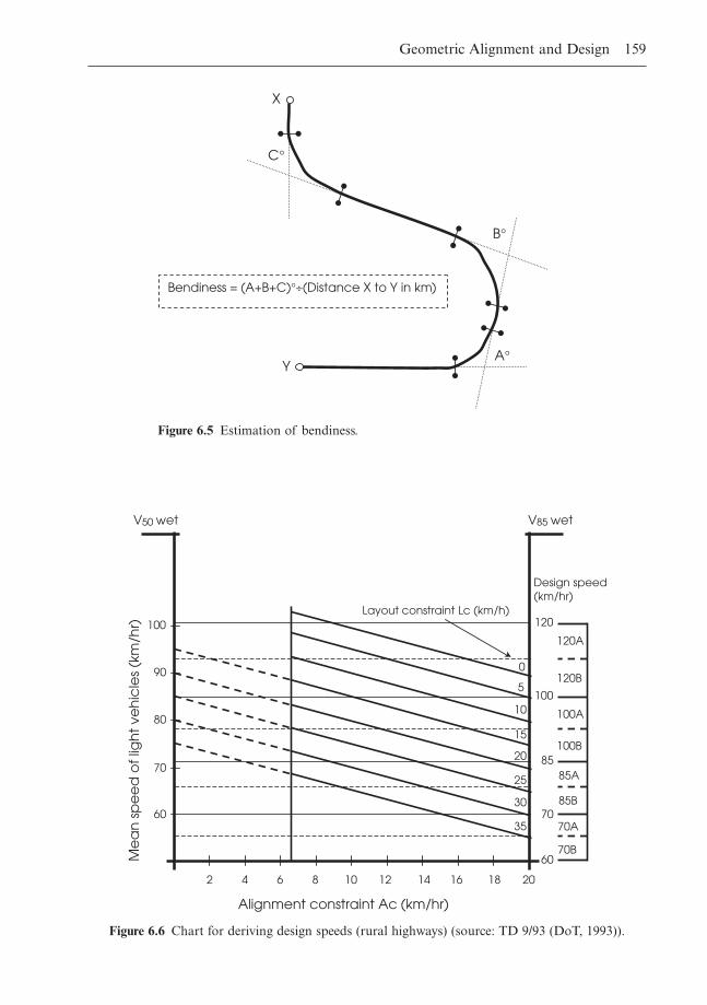
Geometric Alignment and Design 159
A∞
X
Y
B∞
C∞
Bendiness = (A+B+C)∞∏(Distance X to Y in km)
Figure 6.5 Estimation of bendiness.
0
Alignment constraint Ac (km/hr)
Me
an
sp
ee
d o
f lig
ht
veh
icle
s (k
m/h
r)
120
100
85
70
60
120A
120B
100A
100B
85A
85B
70A
70B
Design speed(km/hr)
Layout constraint Lc (km/h)
2 4 6 8 10 12 14 16 18 20
100
90
80
70
60
V50 wet V85 wet
5
10
15
20
25
30
35
Figure 6.6 Chart for deriving design speeds (rural highways) (source: TD 9/93 (DoT, 1993)).
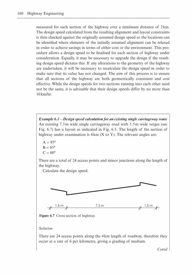
measured for each section of the highway over a minimum distance of 2km.The design speed calculated from the resulting alignment and layout constraintsis then checked against the originally assumed design speed so the locations canbe identified where elements of the initially assumed alignment can be relaxedin order to achieve savings in terms of either cost or the environment. This pro-cedure allows a design speed to be finalised for each section of highway underconsideration. Equally, it may be necessary to upgrade the design if the result-ing design speed dictates this. If any alterations to the geometry of the highwayare undertaken, it will be necessary to recalculate the design speed in order tomake sure that its value has not changed. The aim of this process is to ensurethat all sections of the highway are both geometrically consistent and cost effective. While the design speeds for two sections running into each other neednot be the same, it is advisable that their design speeds differ by no more than10km/hr.
160 Highway Engineering
Example 6.1 – Design speed calculation for an existing single carriageway routeAn existing 7.3m wide single carriageway road with 1.5m wide verges (seeFig. 6.7) has a layout as indicated in Fig. 6.5. The length of the section ofhighway under examination is 4km (X to Y). The relevant angles are:
A = 95°B = 65°C = 60°
There are a total of 24 access points and minor junctions along the length ofthe highway.
Calculate the design speed.
1.5 m 1.5 m 7.3 m
Figure 6.7 Cross-section of highway.
Solution
There are 24 access points along the 4km length of roadway, therefore theyoccur at a rate of 6 per kilometre, giving a grading of medium.
Contd
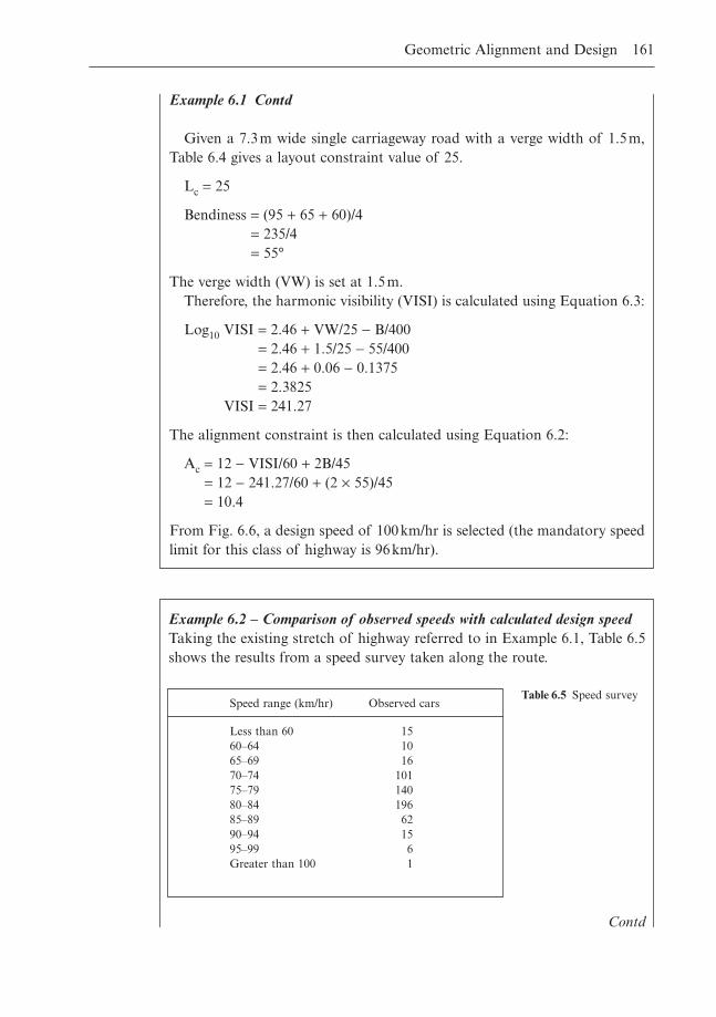
Geometric Alignment and Design 161
Example 6.1 Contd
Given a 7.3m wide single carriageway road with a verge width of 1.5m,Table 6.4 gives a layout constraint value of 25.
Lc = 25
Bendiness = (95 + 65 + 60)/4= 235/4= 55°
The verge width (VW) is set at 1.5m.Therefore, the harmonic visibility (VISI) is calculated using Equation 6.3:
Log10 VISI = 2.46 + VW/25 - B/400= 2.46 + 1.5/25 - 55/400= 2.46 + 0.06 - 0.1375= 2.3825
VISI = 241.27
The alignment constraint is then calculated using Equation 6.2:
Ac = 12 - VISI/60 + 2B/45= 12 - 241.27/60 + (2 ¥ 55)/45= 10.4
From Fig. 6.6, a design speed of 100km/hr is selected (the mandatory speedlimit for this class of highway is 96km/hr).
Example 6.2 – Comparison of observed speeds with calculated design speedTaking the existing stretch of highway referred to in Example 6.1, Table 6.5shows the results from a speed survey taken along the route.
Speed range (km/hr) Observed cars
Less than 60 1560–64 1065–69 1670–74 10175–79 14080–84 19685–89 6290–94 1595–99 6Greater than 100 1
Table 6.5 Speed survey
Contd
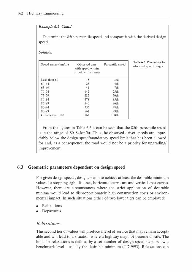
6.3 Geometric parameters dependent on design speed
For given design speeds, designers aim to achieve at least the desirable minimumvalues for stopping sight distance, horizontal curvature and vertical crest curves.However, there are circumstances where the strict application of desirableminima would lead to disproportionately high construction costs or environ-mental impact. In such situations either of two lower tiers can be employed:
� Relaxations� Departures.
Relaxations
This second tier of values will produce a level of service that may remain accept-able and will lead to a situation where a highway may not become unsafe. Thelimit for relaxations is defined by a set number of design speed steps below abenchmark level – usually the desirable minimum (TD 9/93). Relaxations can
162 Highway Engineering
Example 6.2 Contd
Determine the 85th percentile speed and compare it with the derived designspeed.
Solution
Speed range (km/hr) Observed cars Percentile speedwith speed within
or below this range
Less than 60 15 3rd60–64 25 4th65–69 41 7th70–74 142 25th75–79 282 50th80–84 478 85th85–89 540 96th90–94 555 98th95–99 561 99thGreater than 100 562 100th
Table 6.6 Percentiles forobserved speed ranges
From the figures in Table 6.6 it can be seen that the 85th percentile speedis in the range of 80–84km/hr. Thus the observed driver speeds are appre-ciably below the design speed/mandatory speed limit that has been allowedfor and, as a consequence, the road would not be a priority for upgrading/improvement.
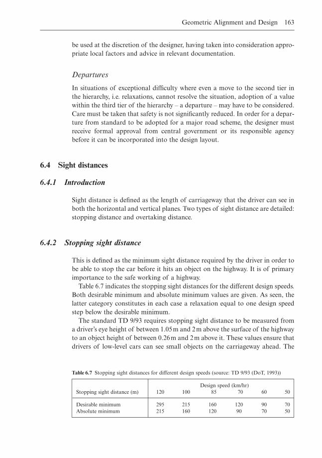
be used at the discretion of the designer, having taken into consideration appro-priate local factors and advice in relevant documentation.
Departures
In situations of exceptional difficulty where even a move to the second tier inthe hierarchy, i.e. relaxations, cannot resolve the situation, adoption of a valuewithin the third tier of the hierarchy – a departure – may have to be considered.Care must be taken that safety is not significantly reduced. In order for a depar-ture from standard to be adopted for a major road scheme, the designer mustreceive formal approval from central government or its responsible agencybefore it can be incorporated into the design layout.
6.4 Sight distances
6.4.1 Introduction
Sight distance is defined as the length of carriageway that the driver can see inboth the horizontal and vertical planes. Two types of sight distance are detailed:stopping distance and overtaking distance.
6.4.2 Stopping sight distance
This is defined as the minimum sight distance required by the driver in order tobe able to stop the car before it hits an object on the highway. It is of primaryimportance to the safe working of a highway.
Table 6.7 indicates the stopping sight distances for the different design speeds.Both desirable minimum and absolute minimum values are given. As seen, thelatter category constitutes in each case a relaxation equal to one design speedstep below the desirable minimum.
The standard TD 9/93 requires stopping sight distance to be measured froma driver’s eye height of between 1.05m and 2m above the surface of the highwayto an object height of between 0.26m and 2m above it. These values ensure thatdrivers of low-level cars can see small objects on the carriageway ahead. The
Geometric Alignment and Design 163
Design speed (km/hr)Stopping sight distance (m) 120 100 85 70 60 50
Desirable minimum 295 215 160 120 90 70Absolute minimum 215 160 120 90 70 50
Table 6.7 Stopping sight distances for different design speeds (source: TD 9/93 (DoT, 1993))
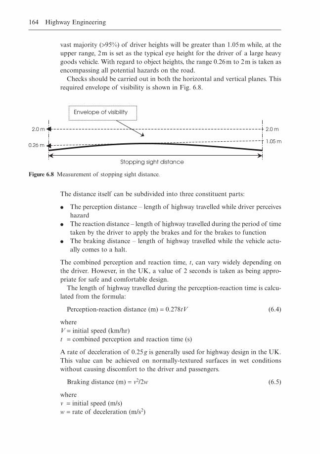
vast majority (>95%) of driver heights will be greater than 1.05m while, at theupper range, 2m is set as the typical eye height for the driver of a large heavygoods vehicle. With regard to object heights, the range 0.26m to 2m is taken asencompassing all potential hazards on the road.
Checks should be carried out in both the horizontal and vertical planes. Thisrequired envelope of visibility is shown in Fig. 6.8.
164 Highway Engineering
2.0 m
0.26 m
2.0 m
1.05 m
Envelope of visibility
Stopping sight distance
Figure 6.8 Measurement of stopping sight distance.
The distance itself can be subdivided into three constituent parts:
� The perception distance – length of highway travelled while driver perceiveshazard
� The reaction distance – length of highway travelled during the period of timetaken by the driver to apply the brakes and for the brakes to function
� The braking distance – length of highway travelled while the vehicle actu-ally comes to a halt.
The combined perception and reaction time, t, can vary widely depending onthe driver. However, in the UK, a value of 2 seconds is taken as being appro-priate for safe and comfortable design.
The length of highway travelled during the perception-reaction time is calcu-lated from the formula:
Perception-reaction distance (m) = 0.278tV (6.4)
whereV = initial speed (km/hr)t = combined perception and reaction time (s)
A rate of deceleration of 0.25g is generally used for highway design in the UK.This value can be achieved on normally-textured surfaces in wet conditionswithout causing discomfort to the driver and passengers.
Braking distance (m) = v2/2w (6.5)
wherev = initial speed (m/s)w = rate of deceleration (m/s2)
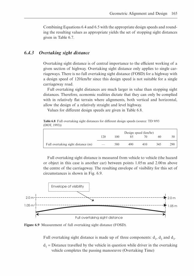
Combining Equations 6.4 and 6.5 with the appropriate design speeds and round-ing the resulting values as appropriate yields the set of stopping sight distancesgiven in Table 6.7.
6.4.3 Overtaking sight distance
Overtaking sight distance is of central importance to the efficient working of agiven section of highway. Overtaking sight distance only applies to single car-riageways. There is no full overtaking sight distance (FOSD) for a highway witha design speed of 120km/hr since this design speed is not suitable for a singlecarriageway road.
Full overtaking sight distances are much larger in value than stopping sightdistances. Therefore, economic realities dictate that they can only be compliedwith in relatively flat terrain where alignments, both vertical and horizontal,allow the design of a relatively straight and level highway.
Values for different design speeds are given in Table 6.8.
Geometric Alignment and Design 165
Design speed (km/hr)120 100 85 70 60 50
Full overtaking sight distance (m) — 580 490 410 345 290
Table 6.8 Full overtaking sight distances for different design speeds (source: TD 9/93 (DOT, 1993))
Full overtaking sight distance is measured from vehicle to vehicle (the hazardor object in this case is another car) between points 1.05m and 2.00m above the centre of the carriageway. The resulting envelope of visibility for this set ofcircumstances is shown in Fig. 6.9.
Full overtaking sight distance
2.0 m 2.0 m
1.05 m
Envelope of visibility
1.05 m
Figure 6.9 Measurement of full overtaking sight distance (FOSD).
Full overtaking sight distance is made up of three components: d1, d2 and d3.
d1 = Distance travelled by the vehicle in question while driver in the overtakingvehicle completes the passing manoeuvre (Overtaking Time)
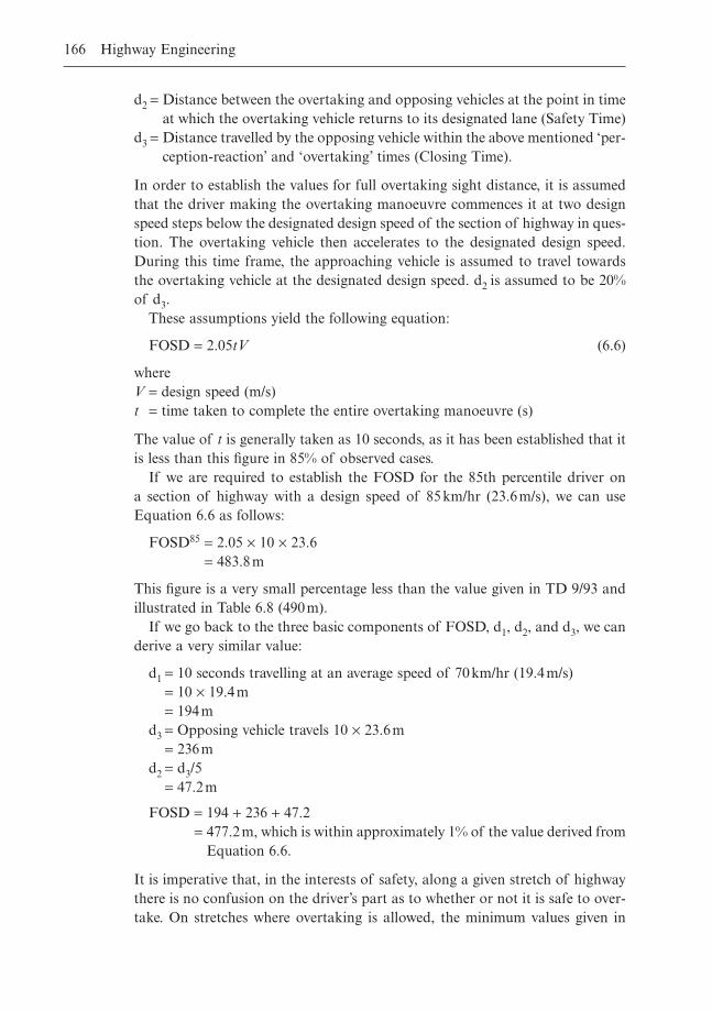
d2 = Distance between the overtaking and opposing vehicles at the point in timeat which the overtaking vehicle returns to its designated lane (Safety Time)
d3 = Distance travelled by the opposing vehicle within the above mentioned ‘per-ception-reaction’ and ‘overtaking’ times (Closing Time).
In order to establish the values for full overtaking sight distance, it is assumedthat the driver making the overtaking manoeuvre commences it at two designspeed steps below the designated design speed of the section of highway in ques-tion. The overtaking vehicle then accelerates to the designated design speed.During this time frame, the approaching vehicle is assumed to travel towardsthe overtaking vehicle at the designated design speed. d2 is assumed to be 20%of d3.
These assumptions yield the following equation:
FOSD = 2.05tV (6.6)
whereV = design speed (m/s)t = time taken to complete the entire overtaking manoeuvre (s)
The value of t is generally taken as 10 seconds, as it has been established that itis less than this figure in 85% of observed cases.
If we are required to establish the FOSD for the 85th percentile driver on a section of highway with a design speed of 85km/hr (23.6m/s), we can useEquation 6.6 as follows:
FOSD85 = 2.05 ¥ 10 ¥ 23.6= 483.8m
This figure is a very small percentage less than the value given in TD 9/93 andillustrated in Table 6.8 (490m).
If we go back to the three basic components of FOSD, d1, d2, and d3, we canderive a very similar value:
d1 = 10 seconds travelling at an average speed of 70km/hr (19.4m/s)= 10 ¥ 19.4m= 194m
d3 = Opposing vehicle travels 10 ¥ 23.6m= 236m
d2 = d3/5= 47.2m
FOSD = 194 + 236 + 47.2= 477.2m, which is within approximately 1% of the value derived from
Equation 6.6.
It is imperative that, in the interests of safety, along a given stretch of highwaythere is no confusion on the driver’s part as to whether or not it is safe to over-take. On stretches where overtaking is allowed, the minimum values given in
166 Highway Engineering
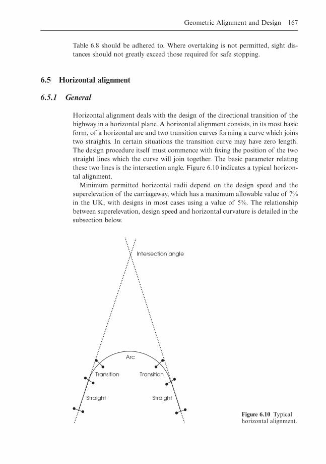
Table 6.8 should be adhered to. Where overtaking is not permitted, sight dis-tances should not greatly exceed those required for safe stopping.
6.5 Horizontal alignment
6.5.1 General
Horizontal alignment deals with the design of the directional transition of thehighway in a horizontal plane. A horizontal alignment consists, in its most basicform, of a horizontal arc and two transition curves forming a curve which joinstwo straights. In certain situations the transition curve may have zero length.The design procedure itself must commence with fixing the position of the twostraight lines which the curve will join together. The basic parameter relatingthese two lines is the intersection angle. Figure 6.10 indicates a typical horizon-tal alignment.
Minimum permitted horizontal radii depend on the design speed and thesuperelevation of the carriageway, which has a maximum allowable value of 7%in the UK, with designs in most cases using a value of 5%. The relationshipbetween superelevation, design speed and horizontal curvature is detailed in thesubsection below.
Geometric Alignment and Design 167
Straight Straight
Transition Transition
Arc
Intersection angle
Figure 6.10 Typicalhorizontal alignment.
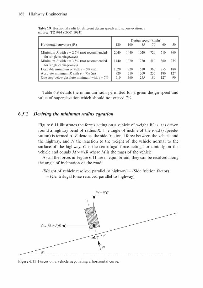
Table 6.9 details the minimum radii permitted for a given design speed andvalue of superelevation which should not exceed 7%.
6.5.2 Deriving the minimum radius equation
Figure 6.11 illustrates the forces acting on a vehicle of weight W as it is drivenround a highway bend of radius R. The angle of incline of the road (superele-vation) is termed a. P denotes the side frictional force between the vehicle andthe highway, and N the reaction to the weight of the vehicle normal to thesurface of the highway. C is the centrifugal force acting horizontally on thevehicle and equals M ¥ v2/R where M is the mass of the vehicle.
As all the forces in Figure 6.11 are in equilibrium, they can be resolved alongthe angle of inclination of the road:
(Weight of vehicle resolved parallel to highway) + (Side friction factor) = (Centrifugal force resolved parallel to highway)
168 Highway Engineering
Design speed (km/hr)Horizontal curvature (R) 120 100 85 70 60 50
Minimum R with e = 2.5% (not recommended 2040 1440 1020 720 510 360for single carriageways)
Minimum R with e = 3.5% (not recommended 1440 1020 720 510 360 255for single carriageways)
Desirable minimum R with e = 5% (m) 1020 720 510 360 255 180Absolute minimum R with e = 7% (m) 720 510 360 255 180 127One step below absolute minimum with e = 7% 510 360 255 180 127 90
Table 6.9 Horizontal radii for different design speeds and superelevation, e(source: TD 9/93 (DOT, 1993))
W = Mg
C = M ¥ v2/R
P
N
a
Figure 6.11 Forces on a vehicle negotiating a horizontal curve.
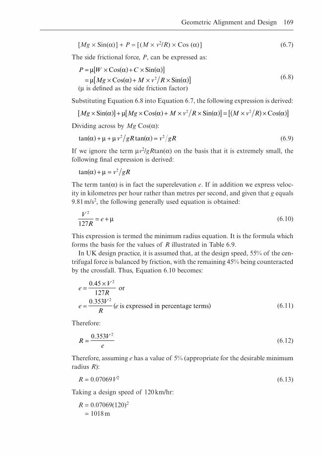
[Mg ¥ Sin(a) ] + P = [ (M ¥ v2/R) ¥ Cos (a) ] (6.7)
The side frictional force, P, can be expressed as:
(6.8)
(m is defined as the side friction factor)
Substituting Equation 6.8 into Equation 6.7, the following expression is derived:
Dividing across by Mg Cos(a):
(6.9)
If we ignore the term mv2/gRtan(a) on the basis that it is extremely small, thefollowing final expression is derived:
The term tan(a) is in fact the superelevation e. If in addition we express veloc-ity in kilometres per hour rather than metres per second, and given that g equals9.81m/s2, the following generally used equation is obtained:
(6.10)
This expression is termed the minimum radius equation. It is the formula whichforms the basis for the values of R illustrated in Table 6.9.
In UK design practice, it is assumed that, at the design speed, 55% of the cen-trifugal force is balanced by friction, with the remaining 45% being counteractedby the crossfall. Thus, Equation 6.10 becomes:
(6.11)
Therefore:
(6.12)
Therefore, assuming e has a value of 5% (appropriate for the desirable minimumradius R):
R = 0.07069V2 (6.13)
Taking a design speed of 120km/hr:
R = 0.07069(120)2
= 1018m
RV
e=
0 353 2.
eV
R
eV
Re
=¥
= ( )
0 45127
0 353
2
2
.
.
or
is expressed in percentage terms
VR
e2
127= + m
tan a m( ) + = v gR2
tan tana m m a( ) + + ( ) =v gR v gR2 2
Mg Mg M v R M v R¥ ( )[ ] + ¥ ( ) + ¥ ¥ ( )[ ] = ¥( ) ¥ ( )[ ]Sin Cos Sin Cosa m a a a2 2
P W C
Mg M v R
= ¥ ( ) + ¥ ( )[ ]= ¥ ( ) + ¥ ¥ ( )[ ]
m a am a a
Cos Sin
Cos Sin2
Geometric Alignment and Design 169
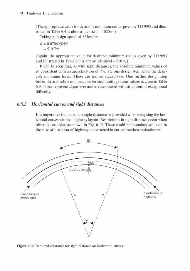
(The appropriate value for desirable minimum radius given by TD 9/93 and illus-trated in Table 6.9 is almost identical – 1020m.)
Taking a design speed of 85km/hr:
R = 0.07069(85)2
= 510.7m
(Again, the appropriate value for desirable minimum radius given by TD 9/93and illustrated in Table 6.9 is almost identical – 510m.)
It can be seen that, as with sight distances, the absolute minimum values ofR, consistent with a superelevation of 7%, are one design step below the desir-able minimum levels. These are termed relaxations. One further design stepbelow these absolute minima, also termed limiting radius values, is given in Table6.9. These represent departures and are associated with situations of exceptionaldifficulty.
6.5.3 Horizontal curves and sight distances
It is imperative that adequate sight distance be provided when designing the hor-izontal curves within a highway layout. Restrictions in sight distance occur whenobstructions exist, as shown in Fig. 6.12. These could be boundary walls or, inthe case of a section of highway constructed in cut, an earthen embankment.
170 Highway Engineering
obstruction
SD
Centreline of highway
Centreline of inside lane
Ms
R R
Ds
Figure 6.12 Required clearance for sight distance on horizontal curves.
The minimum offset clearance Ms required between the centreline of thehighway and the obstruction in question can be estimated in terms of therequired sight distance SD and the radius of curvature of the vehicle’s path Ras follows.
It is assumed that the sight distance lies within the length of the horizontalcurve. The degree of curve is defined as the angle subtended by a 100m long arcalong the horizontal curve. It measures the sharpness of the curve and can berelated to the radius of the curve as follows:
D = 5729.6 ∏ R (6.14)
An analysis of the geometry yields the following formula relating the length ofa curve to the degree of curve:
L = 100 ¥ Ds ∏ D (6.15)
where D is the central angle of the curve.Assuming in this case that the length of the curve is SD, Equation 6.15 can bewritten:
SD = 100 ¥ Ds ∏ D (6.16)
Substituting Equation 6.14 into the above equation yields:
(6.17)
Since:
Therefore:
(6.18)
Substituting Equation 6.17 into 6.18 the following equation is obtained:
(6.19)Ms Cos SD R= - ¥( )[ ]R 1 28 65.
Ms Cos s= - ( )[ ]R 1 2D
Coss
MsD2
ÊË
ˆ¯ = -( ) ∏R R
Ds SD= ¥ ∏57 296. R
Geometric Alignment and Design 171
Example 6.3A 2-lane 7.3m wide single carriageway road has a curve radius of 600m. Theminimum sight stopping distance required is 160m.
Calculate the required distance to be kept clear of obstructions in metres.
Solution
Applying Equation 6.19:
Ms = 600[1 - Cos(28.65 ¥ 160/600)]= 5.33m
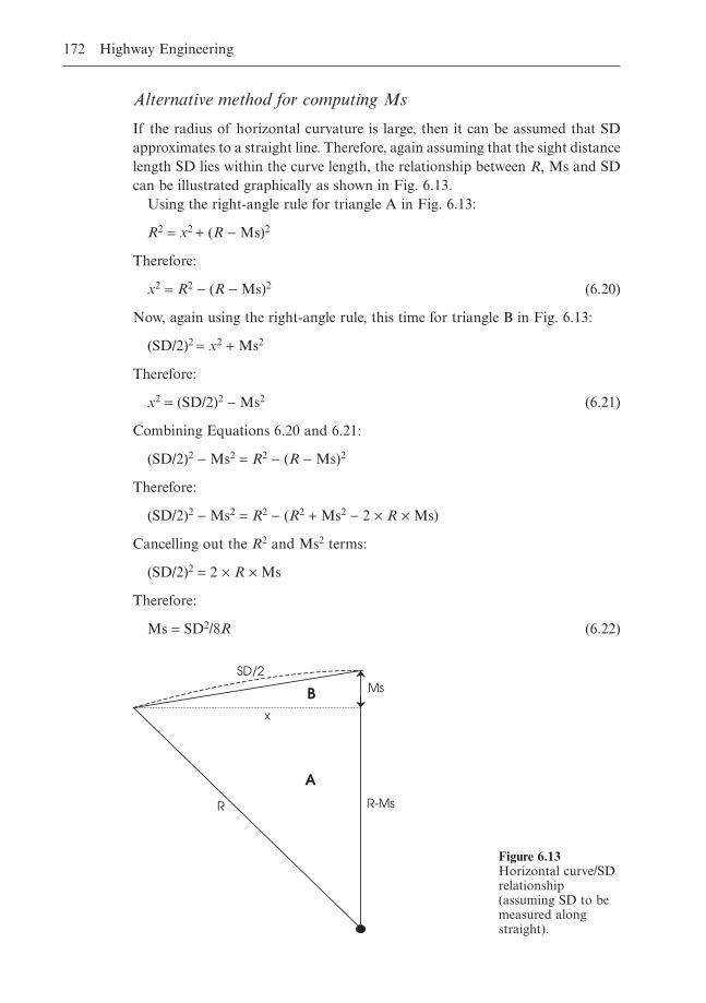
Alternative method for computing Ms
If the radius of horizontal curvature is large, then it can be assumed that SDapproximates to a straight line. Therefore, again assuming that the sight distancelength SD lies within the curve length, the relationship between R, Ms and SDcan be illustrated graphically as shown in Fig. 6.13.
Using the right-angle rule for triangle A in Fig. 6.13:
R2 = x2 + (R - Ms)2
Therefore:
x2 = R2 - (R - Ms)2 (6.20)
Now, again using the right-angle rule, this time for triangle B in Fig. 6.13:
(SD/2)2 = x2 + Ms2
Therefore:
x2 = (SD/2)2 - Ms2 (6.21)
Combining Equations 6.20 and 6.21:
(SD/2)2 - Ms2 = R2 - (R - Ms)2
Therefore:
(SD/2)2 - Ms2 = R2 - (R2 + Ms2 - 2 ¥ R ¥ Ms)
Cancelling out the R2 and Ms2 terms:
(SD/2)2 = 2 ¥ R ¥ Ms
Therefore:
Ms = SD2/8R (6.22)
172 Highway Engineering
SD/2
R
Ms
R-Ms
x
A
B
Figure 6.13Horizontal curve/SDrelationship(assuming SD to bemeasured alongstraight).
If the sight distance length SD lies outside the curve length R, the followingformula can be derived for estimating the minimum offset clearance:
Ms = L(2 ¥ SD - L)/8R (6.23)
For a derivation of this equation, see O’Flaherty (1986).
6.5.4 Transitions
These curve types are used to connect curved and straight sections of highway.(They can also be used to ease the change between two circular curves wherethe difference in radius is large.) The purpose of transition curves is to permitthe gradual introduction of centrifugal forces. Such forces are required in orderto cause a vehicle to move round a circular arc rather than continue in a straightline. A finite quantity of time, long enough for the purposes of ease and safety,will be required by the driver to turn the steering wheel. The vehicle will followits own transition curve as the driver turns the steering wheel. The radial accel-eration experienced by the vehicle travelling at a given velocity v changes fromzero on the tangent to v2/R when on the circular arc. The form of the transitioncurve should be such that the radial acceleration is constant.
The radius of curvature of a transition curve gradually decreases from infinity at the intersection of the tangent and the transition curve to the designated radius R at the intersection of the transition curve with the circularcurve.
Transition curves are normally of spiral or clothoid form:
RL = A2
whereA2 is a constant that controls the scale of the clothoidR is the radius of the horizontal curveL is the length of the clothoid
Geometric Alignment and Design 173
Example 6.4Using the same data as in Example 6.3, calculate the value of Ms using theapproximate method.
Solution
Applying Equation 6.22:
Ms = 1602/(8 ¥ 600)= 25600/4800= 5.33m
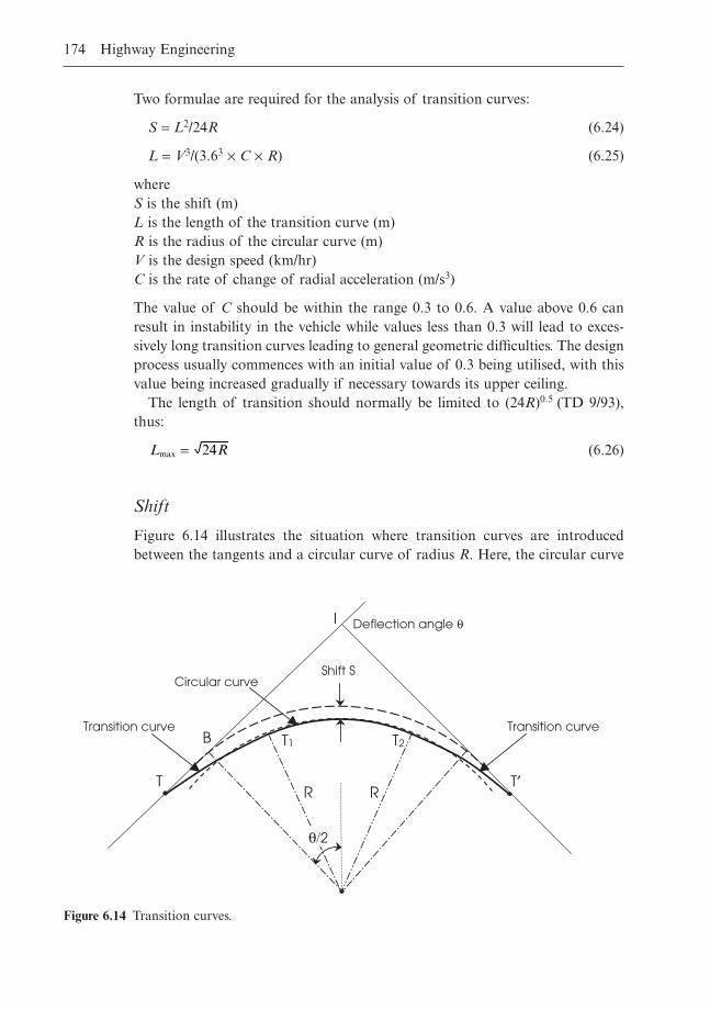
Two formulae are required for the analysis of transition curves:
S = L2/24R (6.24)
L = V3/(3.63 ¥ C ¥ R) (6.25)
whereS is the shift (m)L is the length of the transition curve (m)R is the radius of the circular curve (m)V is the design speed (km/hr)C is the rate of change of radial acceleration (m/s3)
The value of C should be within the range 0.3 to 0.6. A value above 0.6 canresult in instability in the vehicle while values less than 0.3 will lead to exces-sively long transition curves leading to general geometric difficulties. The designprocess usually commences with an initial value of 0.3 being utilised, with thisvalue being increased gradually if necessary towards its upper ceiling.
The length of transition should normally be limited to (24R)0.5 (TD 9/93),thus:
(6.26)
Shift
Figure 6.14 illustrates the situation where transition curves are introducedbetween the tangents and a circular curve of radius R. Here, the circular curve
L Rmax = 24
174 Highway Engineering
Deflection angle qI
T T¢
T1 T2
R R
Shift S
Transition curve Transition curve
Circular curve
B
q/2
Figure 6.14 Transition curves.
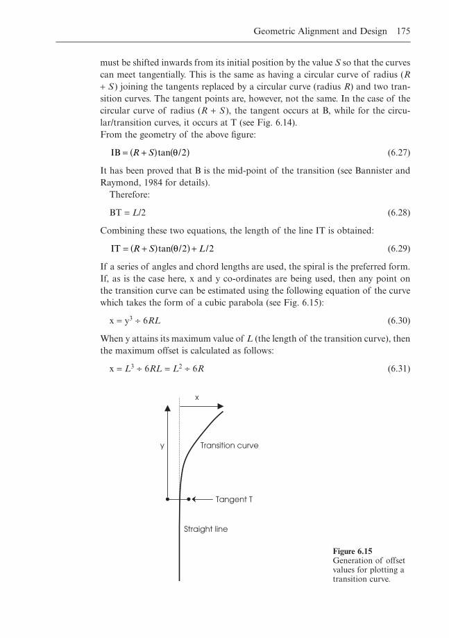
must be shifted inwards from its initial position by the value S so that the curvescan meet tangentially. This is the same as having a circular curve of radius (R+ S ) joining the tangents replaced by a circular curve (radius R) and two tran-sition curves. The tangent points are, however, not the same. In the case of thecircular curve of radius (R + S ), the tangent occurs at B, while for the circu-lar/transition curves, it occurs at T (see Fig. 6.14).From the geometry of the above figure:
(6.27)
It has been proved that B is the mid-point of the transition (see Bannister andRaymond, 1984 for details).
Therefore:
BT = L/2 (6.28)
Combining these two equations, the length of the line IT is obtained:
(6.29)
If a series of angles and chord lengths are used, the spiral is the preferred form.If, as is the case here, x and y co-ordinates are being used, then any point onthe transition curve can be estimated using the following equation of the curvewhich takes the form of a cubic parabola (see Fig. 6.15):
x = y3 ∏ 6RL (6.30)
When y attains its maximum value of L (the length of the transition curve), thenthe maximum offset is calculated as follows:
x = L3 ∏ 6RL = L2 ∏ 6R (6.31)
IT = +( ) ( ) +R S Ltan / /q 2 2
IB = +( ) ( )R S tan /q 2
Geometric Alignment and Design 175
y
x
Straight line
Transition curve
Tangent T
Figure 6.15Generation of offsetvalues for plotting atransition curve.
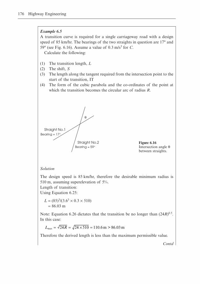
176 Highway Engineering
Example 6.5A transition curve is required for a single carriageway road with a designspeed of 85 km/hr. The bearings of the two straights in question are 17° and59° (see Fig. 6.16). Assume a value of 0.3 m/s3 for C.
Calculate the following:
(1) The transition length, L(2) The shift, S(3) The length along the tangent required from the intersection point to the
start of the transition, IT(4) The form of the cubic parabola and the co-ordinates of the point at
which the transition becomes the circular arc of radius R.
Contd
q
Straight No.1
Straight No.2
Bearing = 17∞
Bearing = 59∞Figure 6.16Intersection angle qbetween straights.
Solution
The design speed is 85 km/hr, therefore the desirable minimum radius is 510 m, assuming superelevation of 5%.Length of transition:Using Equation 6.25:
L = (85)3/(3.63 ¥ 0.3 ¥ 510)= 86.03 m
Note: Equation 6.26 dictates that the transition be no longer than (24R)0.5.In this case:
Therefore the derived length is less than the maximum permissible value.
L Rmax .= = ¥ =24 24 510 110 6 m > 86.03 m
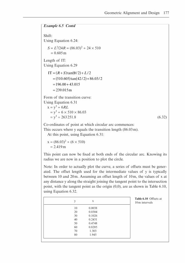
Geometric Alignment and Design 177
Example 6.5 Contd
Shift:Using Equation 6.24:
S = L2/24R = (86.03)2 ∏ 24 ¥ 510= 0.605m
Length of IT:Using Equation 6.29
Form of the transition curve:Using Equation 6.31
x = y3 ∏ 6RL= y3 ∏ 6 ¥ 510 ¥ 86.03= y3 ∏ 263251.8 (6.32)
Co-ordinates of point at which circular arc commences:This occurs where y equals the transition length (86.03m).
At this point, using Equation 6.31:
x = (86.03)2 ∏ (6 ¥ 510)= 2.419m
This point can now be fixed at both ends of the circular arc. Knowing itsradius we are now in a position to plot the circle.
Note: In order to actually plot the curve, a series of offsets must be gener-ated. The offset length used for the intermediate values of y is typicallybetween 10 and 20m. Assuming an offset length of 10m, the values of x atany distance y along the straight joining the tangent point to the intersectionpoint, with the tangent point as the origin (0,0), are as shown in Table 6.10,using Equation 6.32.
IT
m
= +( ) ( ) += ( ) ( ) += +=
R S Ltan / /
. tan / . /
. .
.
q 2 2
510 605 42 2 86 03 2
196 00 43 015
239 015
y x
10 0.003820 0.030430 0.102640 0.243150 0.474860 0.820570 1.30380 1.945
Table 6.10 Offsets at 10m intervals
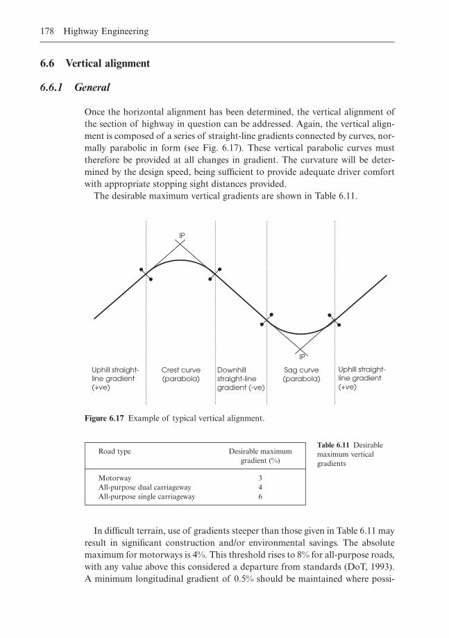
6.6 Vertical alignment
6.6.1 General
Once the horizontal alignment has been determined, the vertical alignment ofthe section of highway in question can be addressed. Again, the vertical align-ment is composed of a series of straight-line gradients connected by curves, nor-mally parabolic in form (see Fig. 6.17). These vertical parabolic curves musttherefore be provided at all changes in gradient. The curvature will be deter-mined by the design speed, being sufficient to provide adequate driver comfortwith appropriate stopping sight distances provided.
The desirable maximum vertical gradients are shown in Table 6.11.
178 Highway Engineering
IP
IP
Uphill straight-line gradient (+ve)
Crest curve (parabola)
Downhill straight-line gradient (-ve)
Sag curve (parabola)
Uphill straight-line gradient (+ve)
Figure 6.17 Example of typical vertical alignment.
Road type Desirable maximumgradient (%)
Motorway 3All-purpose dual carriageway 4All-purpose single carriageway 6
Table 6.11 Desirablemaximum verticalgradients
In difficult terrain, use of gradients steeper than those given in Table 6.11 mayresult in significant construction and/or environmental savings. The absolutemaximum for motorways is 4%. This threshold rises to 8% for all-purpose roads,with any value above this considered a departure from standards (DoT, 1993).A minimum longitudinal gradient of 0.5% should be maintained where possi-
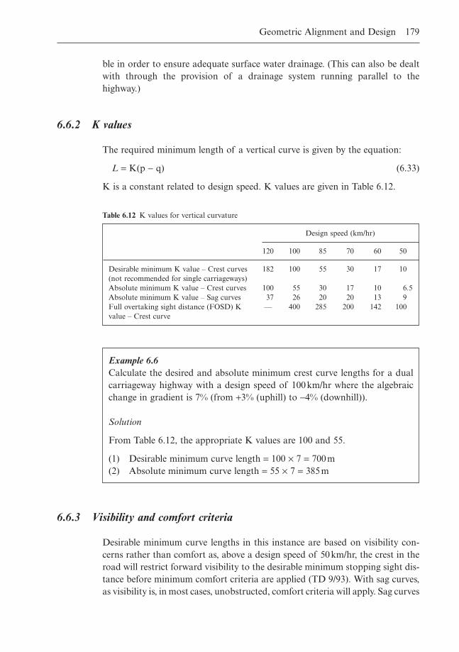
ble in order to ensure adequate surface water drainage. (This can also be dealtwith through the provision of a drainage system running parallel to thehighway.)
6.6.2 K values
The required minimum length of a vertical curve is given by the equation:
L = K(p - q) (6.33)
K is a constant related to design speed. K values are given in Table 6.12.
Geometric Alignment and Design 179
Design speed (km/hr)
120 100 85 70 60 50
Desirable minimum K value – Crest curves 182 100 55 30 17 10(not recommended for single carriageways)Absolute minimum K value – Crest curves 100 55 30 17 10 6.5Absolute minimum K value – Sag curves 37 26 20 20 13 9Full overtaking sight distance (FOSD) K — 400 285 200 142 100value – Crest curve
Table 6.12 K values for vertical curvature
Example 6.6Calculate the desired and absolute minimum crest curve lengths for a dualcarriageway highway with a design speed of 100km/hr where the algebraicchange in gradient is 7% (from +3% (uphill) to -4% (downhill)).
Solution
From Table 6.12, the appropriate K values are 100 and 55.
(1) Desirable minimum curve length = 100 ¥ 7 = 700m(2) Absolute minimum curve length = 55 ¥ 7 = 385m
6.6.3 Visibility and comfort criteria
Desirable minimum curve lengths in this instance are based on visibility con-cerns rather than comfort as, above a design speed of 50km/hr, the crest in theroad will restrict forward visibility to the desirable minimum stopping sight dis-tance before minimum comfort criteria are applied (TD 9/93). With sag curves,as visibility is, in most cases, unobstructed, comfort criteria will apply. Sag curves
should therefore normally be designed to the absolute minimum K valuedetailed in Table 6.12. For both crest and sag curves, relaxations below thedesired minimum values may be made at the discretion of the designer, thoughthe number of design steps permitted below the desirable minimum value willvary depending on the curve and road type, as shown in Table 6.13.
180 Highway Engineering
Road type Crest curve Sag curve
Motorway 1 or 2 steps 0 stepsAll-purpose 2 or 3 steps 1 or 2 steps
Table 6.13 Permittedrelaxations for differentroad and vertical curvetypes (below desiredmin. for crest curvesand below absolute min.for sag curves)
6.6.4 Parabolic formula
Referring to Fig. 6.18, the formula for determining the co-ordinates of pointsalong a typical vertical curve is:
(6.34)
wherep and q are the gradients of the two straights being joined by the vertical curvein question.L is the vertical curve lengthx and y are the relevant co-ordinates in space
Proof
If Y is taken as the elevation of the curve at a point x along the parabola, then:
(6.35)
Integrating Equation 6.35:
(6.36)
Examining the boundary conditions:When x = 0:
(6.37)
(p being the slope of the first straight line gradient)Therefore:
p = C (6.38)
dYdx
p=
dYdx
kx C= +
d Ydx
k a constant2
2 = ( )
yq p2
x2=-È
Î͢˚̇L
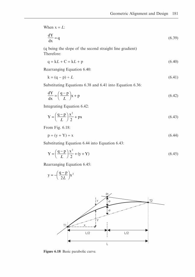
When x = L:
(6.39)
(q being the slope of the second straight line gradient)Therefore:
q = kL + C = kL + p (6.40)
Rearranging Equation 6.40:
k = (q - p) ∏ L (6.41)
Substituting Equations 6.38 and 6.41 into Equation 6.36:
(6.42)
Integrating Equation 6.42:
(6.43)
From Fig. 6.18:
p = (y + Y) ∏ x (6.44)
Substituting Equation 6.44 into Equation 6.43:
(6.45)
Rearranging Equation 6.45:
yq p2
x 2= --Ê
ˈ¯L
Yq p x
2y Y
2
=-Ê
ˈ¯ + +( )
L
Yq p x
2px
2
=-Ê
ˈ¯ +
L
dYdx
q px p=
-ÊË
ˆ¯ +
L
dYdx
q=
Geometric Alignment and Design 181
Y
x
PI
T1
T2
L
L/2 L/2
e
e
y
Figure 6.18 Basic parabolic curve.
where x is the distance along the curve measured from the start of the verticalcurve and y is the vertical offset measured from the continuation of the slopeto the curve.
At the intersection point PI:
x = L/2
Therefore
(6.46)
The co-ordinates of the highest/lowest point on the parabolic curve, frequentlyrequired for the estimation of minimum sight distance requirements, are:
(6.47)
(6.48)yp
2 p q
2
=-( )
L
xp
p q=
-L
eq p2L 2
y
q p8
2
= --Ê
ˈ¯ÊË
ˆ¯ =
= - -( )
L
L
182 Highway Engineering
Example 6.7A vertical alignment for a single carriageway road consists of a paraboliccrest curve connecting a straight-line uphill gradient of +4% with a straight-line downhill gradient of -3%.
(1) Calculate the vertical offset at the point of intersection of the two tangents at PI
(2) Calculate the vertical and horizontal offsets for the highest point on thecurve.
Assume a design speed of 85km/hr and use the absolute minimum K valuefor crest curves.
Solution
Referring to Table 6.12, a K value of 30 is obtained. This gives an absoluteminimum curve length of 210m.
Vertical offset at PI:p = +4%q = -3%
Contd
6.6.5 Crossfalls
To ensure adequate rainfall run-off from the surface of the highway, a minimumcrossfall of 2.5% is advised, either in the form of a straight camber extendingfrom one edge of the carriageway to the other or as one sloped from the centreof the carriageway towards both edges (see Fig. 6.19).
6.6.6 Vertical crest curve design and sight distance requirements
In the case of a crest curve, the intervening highway pavement obstructs the vis-ibility between driver and object. The curvature of crest curves should be suffi-ciently large in order to provide adequate sight distance for the driver. In orderto provide this sight distance, the curve length L is a critical parameter. Toogreat a length is costly to the developer while too short a length compromisescritical concerns such as safety and vertical clearance to structures.
For vertical crest curves, the relevant parameters are:
� The sight distance S� The length of the curve L
Geometric Alignment and Design 183
Example 6.7 Contd
Using Equation 6.46:
Co-ordinates of highest point on crest curve:Using Equations 6.47 and 6.48
Since, from Equation 6.44
p = (y + Y) ∏ xY = px - y
= 0.04(120) - 2.4= 2.4m
xp
p q210 0.04 0.04 0.03
120 m
yp
2 p q210 0.04 2 0.04
2.4 m
22
=-
= ¥( ) ∏ +( )
=
=-( ) = ¥( ) ∏ ¥ +( )
=
L
L0 03.
e q p8
0.03 0.04 210 8
8375 m
= - -( ) = - - - ( ) ¥( ) ∏
=
L
1.
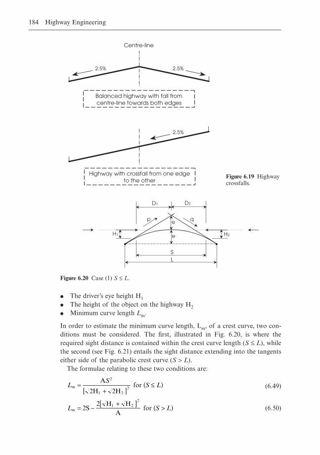
� The driver’s eye height H1� The height of the object on the highway H2� Minimum curve length Lm.
In order to estimate the minimum curve length, Lm, of a crest curve, two con-ditions must be considered. The first, illustrated in Fig. 6.20, is where therequired sight distance is contained within the crest curve length (S £ L), whilethe second (see Fig. 6.21) entails the sight distance extending into the tangentseither side of the parabolic crest curve (S > L).
The formulae relating to these two conditions are:
(6.49)
(6.50)L S Lm1 2
2
2S2 H H
A for = -
+[ ] >( )
LS
S Lm
2
1 2
A
2H 2H for =
+[ ]£( )2
184 Highway Engineering
Balanced highway with fall from centre-line towards both edges
Centre-line
2.5%2.5%
2.5%
Highway with crossfall from one edge to the other
Figure 6.19 Highwaycrossfalls.
D1 D2
H1 H2
SL
e
e
p q
Figure 6.20 Case (1) S £ L.
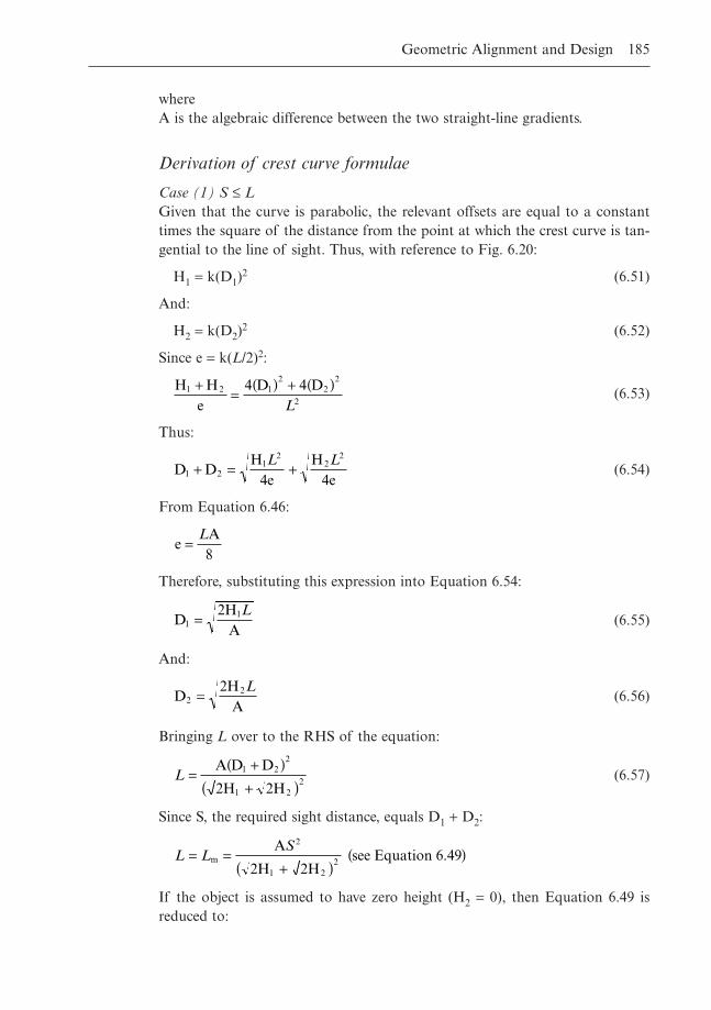
whereA is the algebraic difference between the two straight-line gradients.
Derivation of crest curve formulae
Case (1) S £ LGiven that the curve is parabolic, the relevant offsets are equal to a constanttimes the square of the distance from the point at which the crest curve is tan-gential to the line of sight. Thus, with reference to Fig. 6.20:
H1 = k(D1)2 (6.51)
And:
H2 = k(D2)2 (6.52)
Since e = k(L/2)2:
(6.53)
Thus:
(6.54)
From Equation 6.46:
Therefore, substituting this expression into Equation 6.54:
(6.55)
And:
(6.56)
Bringing L over to the RHS of the equation:
(6.57)
Since S, the required sight distance, equals D1 + D2:
If the object is assumed to have zero height (H2 = 0), then Equation 6.49 isreduced to:
L LS
= =+( )
( )m
2
1 22
A
2H 2H see Equation 6.49
L =+( )
+( )A D D
2H 2H
1 22
1 22
D2H
A22=L
D2H
A11=L
eA8
=L
D DH
4eH
4e1 21
22
2
+ = +L L
H He
4 D 4 D1 2 12
22
2
+=
( ) + ( )L
Geometric Alignment and Design 185
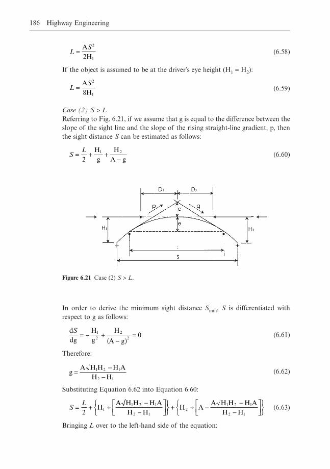
(6.58)
If the object is assumed to be at the driver’s eye height (H1 = H2):
(6.59)
Case (2) S > LReferring to Fig. 6.21, if we assume that g is equal to the difference between theslope of the sight line and the slope of the rising straight-line gradient, p, thenthe sight distance S can be estimated as follows:
(6.60)SL
= + +-2
Hg
HA g
1 2
LS
=A8H
2
1
LS
=A2H
2
1
186 Highway Engineering
Figure 6.21 Case (2) S > L.
In order to derive the minimum sight distance Smin, S is differentiated withrespect to g as follows:
(6.61)
Therefore:
(6.62)
Substituting Equation 6.62 into Equation 6.60:
(6.63)
Bringing L over to the left-hand side of the equation:
SL
= + ∏-
-ÈÎÍ
˘˚̇
ÏÌÓ
¸˝˛
+ ∏ --
-ÈÎÍ
˘˚̇
ÏÌÓ
¸˝˛2
HA H H H A
H HH A
A H H H AH H1
1 2 1
2 12
1 2 1
2 1
gA H H H A
H H1 2 1
2 1
=-
-
ddg
Hg
H
A g01
22
2
S= - +
-( )=
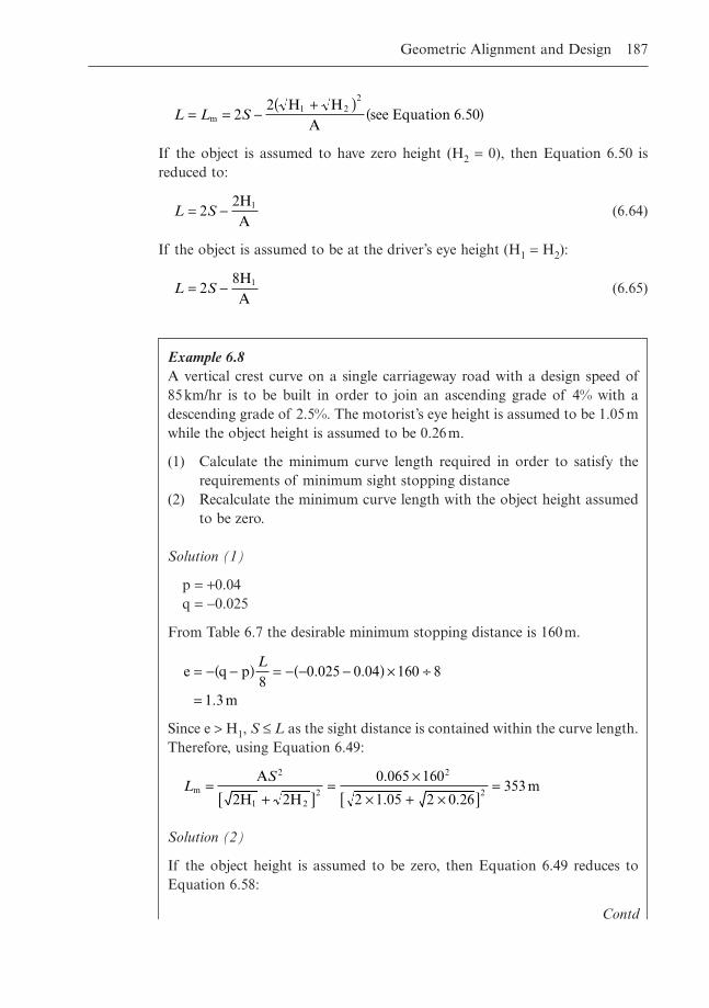
If the object is assumed to have zero height (H2 = 0), then Equation 6.50 isreduced to:
(6.64)
If the object is assumed to be at the driver’s eye height (H1 = H2):
(6.65)L S= -28HA
1
L S= -22HA
1
L L S= = -+( ) ( )m
1 22
22 H H
Asee Equation 6.50
Geometric Alignment and Design 187
Example 6.8A vertical crest curve on a single carriageway road with a design speed of85km/hr is to be built in order to join an ascending grade of 4% with adescending grade of 2.5%. The motorist’s eye height is assumed to be 1.05mwhile the object height is assumed to be 0.26m.
(1) Calculate the minimum curve length required in order to satisfy therequirements of minimum sight stopping distance
(2) Recalculate the minimum curve length with the object height assumedto be zero.
Solution (1)
p = +0.04q = -0.025
From Table 6.7 the desirable minimum stopping distance is 160m.
Since e > H1, S £ L as the sight distance is contained within the curve length.Therefore, using Equation 6.49:
Solution (2)
If the object height is assumed to be zero, then Equation 6.49 reduces toEquation 6.58:
LS
m
2
1 22
2
2
A
2H 2H
0.065 160
2 1.05 2 0.26m=
+[ ]=
¥¥ + ¥[ ]
= 353
e q p8
0.025 0.04 160 8
1.3 m
= - -( ) = - - -( ) ¥ ∏
=
L
Contd

188 Highway Engineering
Example 6.8 Contd
Thus the required crest curve length more than doubles in value if the objectheight is reduced to zero.
LS
= =¥
¥=
A2H
0.065 1602 1.05
792 m
2
1
2
Example 6.9Using the same basic data as Example 6.8, but with the following straight-line gradients:
p = +0.02q = -0.02
calculate the required curve length assuming a motorist’s eye height of1.05m and an object height of 0.26m.
Solution
In this case:
Given that in this case e < H1, S > L as the sight distance is greater than thecurve length.Therefore, using Equation 6.49:
Note: if the object height is reduced to zero, then the required curve lengthis calculated from Equation 6.64:
L S= - = ¥ -¥
= -=
22HA
2 1602 1.05
0.04320 52.5
267.5 m
1
L Sm1 2
2 2
22 H H
A2 160
2 1.05 0.260.04
320 117.75
202.25 m
= -+[ ] = ¥ -
+[ ]
= -=
e q p8
0.02 0.02 160 8
0.8 m
= - -( ) = - - -( ) ¥ ∏
=
L
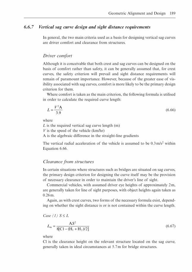
6.6.7 Vertical sag curve design and sight distance requirements
In general, the two main criteria used as a basis for designing vertical sag curvesare driver comfort and clearance from structures.
Driver comfort
Although it is conceivable that both crest and sag curves can be designed on thebasis of comfort rather than safety, it can be generally assumed that, for crestcurves, the safety criterion will prevail and sight distance requirements willremain of paramount importance. However, because of the greater ease of vis-ibility associated with sag curves, comfort is more likely to be the primary designcriterion for them.
Where comfort is taken as the main criterion, the following formula is utilisedin order to calculate the required curve length:
(6.66)
whereL is the required vertical sag curve length (m)V is the speed of the vehicle (km/hr)A is the algebraic difference in the straight-line gradients
The vertical radial acceleration of the vehicle is assumed to be 0.3m/s2 withinEquation 6.66.
Clearance from structures
In certain situations where structures such as bridges are situated on sag curves,the primary design criterion for designing the curve itself may be the provisionof necessary clearance in order to maintain the driver’s line of sight.
Commercial vehicles, with assumed driver eye heights of approximately 2m,are generally taken for line of sight purposes, with object heights again taken as0.26m.
Again, as with crest curves, two forms of the necessary formula exist, depend-ing on whether the sight distance is or is not contained within the curve length.
Case (1) S £ L
(6.67)
whereCl is the clearance height on the relevant structure located on the sag curve,generally taken in ideal circumstances at 5.7m for bridge structures.
LS
m
2
1 2
A8 C1 H H /2
=- +( )[ ]
LV
=2A
3.9
Geometric Alignment and Design 189
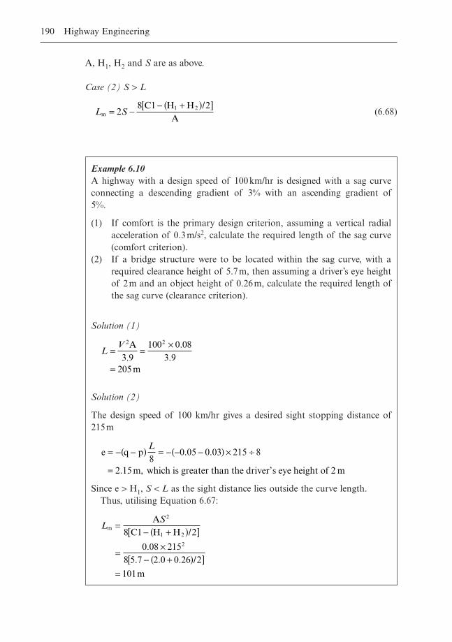
A, H1, H2 and S are as above.
Case (2) S > L
(6.68)L Sm1 22
8 C1 H H /2A
= -- +( )[ ]
190 Highway Engineering
Example 6.10A highway with a design speed of 100km/hr is designed with a sag curve connecting a descending gradient of 3% with an ascending gradient of5%.
(1) If comfort is the primary design criterion, assuming a vertical radialacceleration of 0.3m/s2, calculate the required length of the sag curve(comfort criterion).
(2) If a bridge structure were to be located within the sag curve, with arequired clearance height of 5.7m, then assuming a driver’s eye heightof 2m and an object height of 0.26m, calculate the required length ofthe sag curve (clearance criterion).
Solution (1)
Solution (2)
The design speed of 100 km/hr gives a desired sight stopping distance of215m
Since e > H1, S < L as the sight distance lies outside the curve length.Thus, utilising Equation 6.67:
LS
m
2
1 2
2
A8 C1 H H /2
0.08 2158 5.7 2.0 0.26 /2
101m
=- +( )[ ]
=¥
- +( )[ ]=
e q p8
0.05 0.03 215 8
2.15 m, which is greater than the driver’s eye height of 2 m
= - -( ) = - - -( ) ¥ ∏
=
L
LV
= =¥
=
2 2A3.9
100 0.083.9
205 m
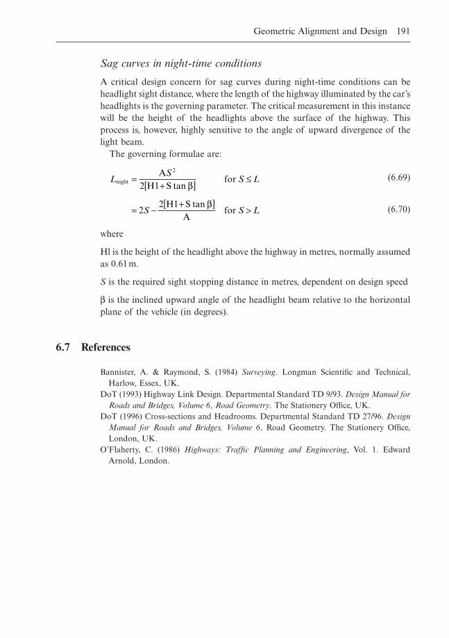
Sag curves in night-time conditions
A critical design concern for sag curves during night-time conditions can beheadlight sight distance, where the length of the highway illuminated by the car’sheadlights is the governing parameter. The critical measurement in this instancewill be the height of the headlights above the surface of the highway. Thisprocess is, however, highly sensitive to the angle of upward divergence of thelight beam.
The governing formulae are:
(6.69)
(6.70)
where
Hl is the height of the headlight above the highway in metres, normally assumedas 0.61m.
S is the required sight stopping distance in metres, dependent on design speed
b is the inclined upward angle of the headlight beam relative to the horizontalplane of the vehicle (in degrees).
6.7 References
Bannister, A. & Raymond, S. (1984) Surveying. Longman Scientific and Technical,Harlow, Essex, UK.
DoT (1993) Highway Link Design. Departmental Standard TD 9/93. Design Manual forRoads and Bridges, Volume 6, Road Geometry. The Stationery Office, UK.
DoT (1996) Cross-sections and Headrooms. Departmental Standard TD 27/96. DesignManual for Roads and Bridges, Volume 6, Road Geometry. The Stationery Office,London, UK.
O’Flaherty, C. (1986) Highways: Traffic Planning and Engineering, Vol. 1. EdwardArnold, London.
LS
S L
S S L
night
2A2 H1 S tan
for
22 H1 S tan
Afor
=+[ ] £
= -+[ ]
>
b
b
Geometric Alignment and Design 191
Chapter 7
Highway Pavement Materials and Design
7.1 Introduction
A highway pavement is composed of a system of overlaid strata of chosenprocessed materials that is positioned on the in-situ soil, termed the subgrade.Its basic requirement is the provision of a uniform skid-resistant running surfacewith adequate life and requiring minimum maintenance. The chief structuralpurpose of the pavement is the support of vehicle wheel loads applied to thecarriageway and the distribution of them to the subgrade immediately under-neath. If the road is in cut, the subgrade will consist of the in-situ soil. If it isconstructed on fill, the top layers of the embankment structure are collectivelytermed the subgrade.
The pavement designer must develop the most economical combination oflayers that will guarantee adequate dispersion of the incident wheel stresses sothat each layer in the pavement does not become overstressed during the designlife of the highway.
The major variables in the design of a highway pavement are:
� The thickness of each layer in the pavement� The material contained within each layer of the pavement� The type of vehicles in the traffic stream� The volume of traffic predicted to use the highway over its design life� The strength of the underlying subgrade soil.
There are three basic components of the highway pavement, general definitionsof which are given here. (More detailed descriptions of their composition appearin the explanations of the two major pavement types later in the chapter.)
Foundation
The foundation consists of the native subgrade soil and the layer of graded stone(subbase and possibly capping) immediately overlaying it. The function of thesubbase and capping is to provide a platform on which to place the roadbasematerial as well as to insulate the subgrade below it against the effects ofinclement weather. These layers may form the temporary road surface usedduring the construction phase of the highway.
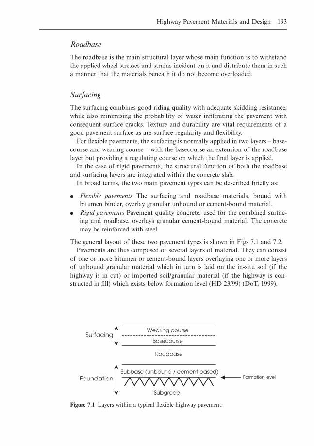
Highway Pavement Materials and Design 193
Roadbase
The roadbase is the main structural layer whose main function is to withstandthe applied wheel stresses and strains incident on it and distribute them in sucha manner that the materials beneath it do not become overloaded.
Surfacing
The surfacing combines good riding quality with adequate skidding resistance,while also minimising the probability of water infiltrating the pavement withconsequent surface cracks. Texture and durability are vital requirements of agood pavement surface as are surface regularity and flexibility.
For flexible pavements, the surfacing is normally applied in two layers – base-course and wearing course – with the basecourse an extension of the roadbaselayer but providing a regulating course on which the final layer is applied.
In the case of rigid pavements, the structural function of both the roadbaseand surfacing layers are integrated within the concrete slab.
In broad terms, the two main pavement types can be described briefly as:
� Flexible pavements The surfacing and roadbase materials, bound withbitumen binder, overlay granular unbound or cement-bound material.
� Rigid pavements Pavement quality concrete, used for the combined surfac-ing and roadbase, overlays granular cement-bound material. The concretemay be reinforced with steel.
The general layout of these two pavement types is shown in Figs 7.1 and 7.2.Pavements are thus composed of several layers of material. They can consist
of one or more bitumen or cement-bound layers overlaying one or more layersof unbound granular material which in turn is laid on the in-situ soil (if thehighway is in cut) or imported soil/granular material (if the highway is con-structed in fill) which exists below formation level (HD 23/99) (DoT, 1999).
Surfacing
Foundation
Wearing course
Basecourse
Roadbase
Subbase (unbound / cement based)
Subgrade
Formation level
Figure 7.1 Layers within a typical flexible highway pavement.
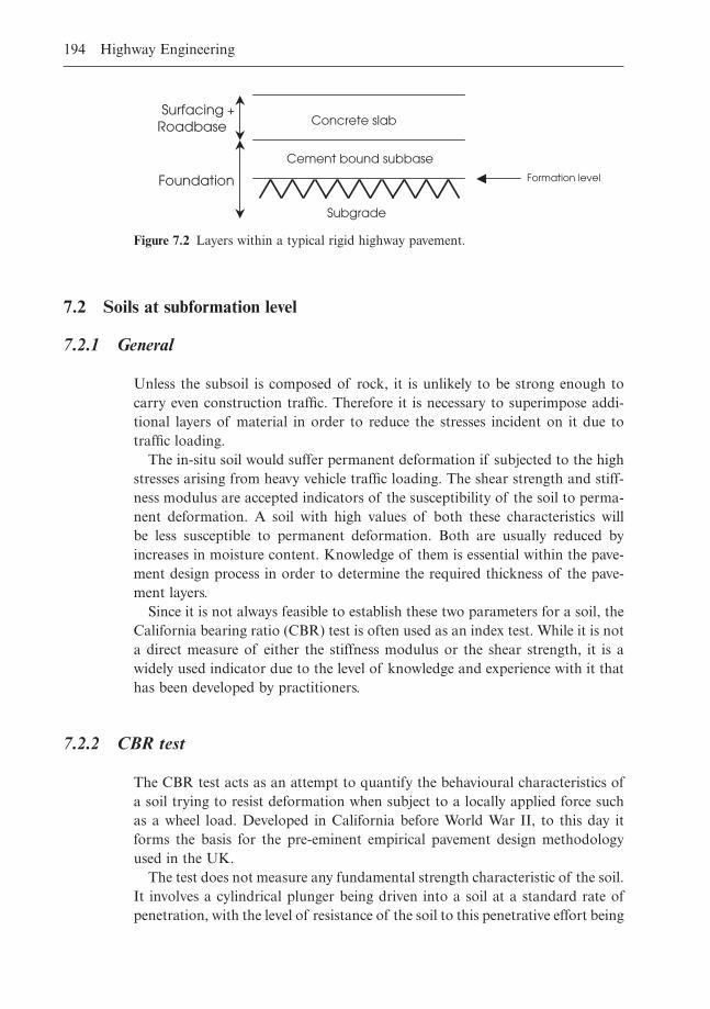
194 Highway Engineering
7.2 Soils at subformation level
7.2.1 General
Unless the subsoil is composed of rock, it is unlikely to be strong enough tocarry even construction traffic. Therefore it is necessary to superimpose addi-tional layers of material in order to reduce the stresses incident on it due totraffic loading.
The in-situ soil would suffer permanent deformation if subjected to the highstresses arising from heavy vehicle traffic loading. The shear strength and stiff-ness modulus are accepted indicators of the susceptibility of the soil to perma-nent deformation. A soil with high values of both these characteristics will be less susceptible to permanent deformation. Both are usually reduced byincreases in moisture content. Knowledge of them is essential within the pave-ment design process in order to determine the required thickness of the pave-ment layers.
Since it is not always feasible to establish these two parameters for a soil, theCalifornia bearing ratio (CBR) test is often used as an index test. While it is nota direct measure of either the stiffness modulus or the shear strength, it is awidely used indicator due to the level of knowledge and experience with it thathas been developed by practitioners.
7.2.2 CBR test
The CBR test acts as an attempt to quantify the behavioural characteristics ofa soil trying to resist deformation when subject to a locally applied force suchas a wheel load. Developed in California before World War II, to this day itforms the basis for the pre-eminent empirical pavement design methodologyused in the UK.
The test does not measure any fundamental strength characteristic of the soil.It involves a cylindrical plunger being driven into a soil at a standard rate ofpenetration, with the level of resistance of the soil to this penetrative effort being
Surfacing + Roadbase
Foundation
Cement bound subbase
Subgrade
Concrete slab
Formation level
Figure 7.2 Layers within a typical rigid highway pavement.
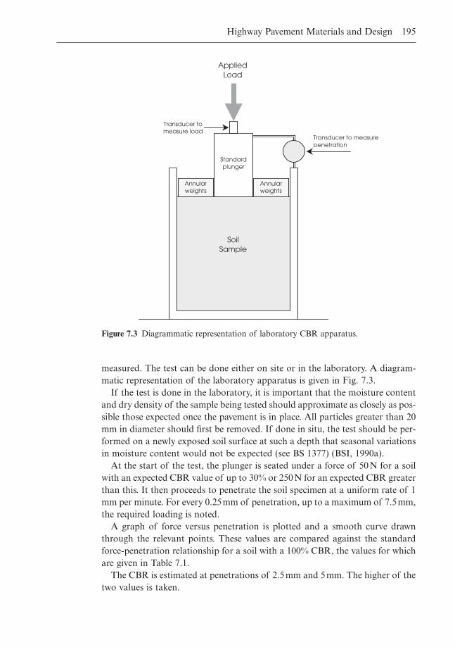
Highway Pavement Materials and Design 195
measured. The test can be done either on site or in the laboratory. A diagram-matic representation of the laboratory apparatus is given in Fig. 7.3.
If the test is done in the laboratory, it is important that the moisture contentand dry density of the sample being tested should approximate as closely as pos-sible those expected once the pavement is in place. All particles greater than 20mm in diameter should first be removed. If done in situ, the test should be per-formed on a newly exposed soil surface at such a depth that seasonal variationsin moisture content would not be expected (see BS 1377) (BSI, 1990a).
At the start of the test, the plunger is seated under a force of 50N for a soilwith an expected CBR value of up to 30% or 250N for an expected CBR greaterthan this. It then proceeds to penetrate the soil specimen at a uniform rate of 1mm per minute. For every 0.25mm of penetration, up to a maximum of 7.5mm,the required loading is noted.
A graph of force versus penetration is plotted and a smooth curve drawnthrough the relevant points. These values are compared against the standardforce-penetration relationship for a soil with a 100% CBR, the values for whichare given in Table 7.1.
The CBR is estimated at penetrations of 2.5mm and 5mm. The higher of thetwo values is taken.
Standard plunger
Applied Load
Soil Sample
Annular weights
Annular weights
Transducer to measure penetration
Transducer to measure load
Figure 7.3 Diagrammatic representation of laboratory CBR apparatus.
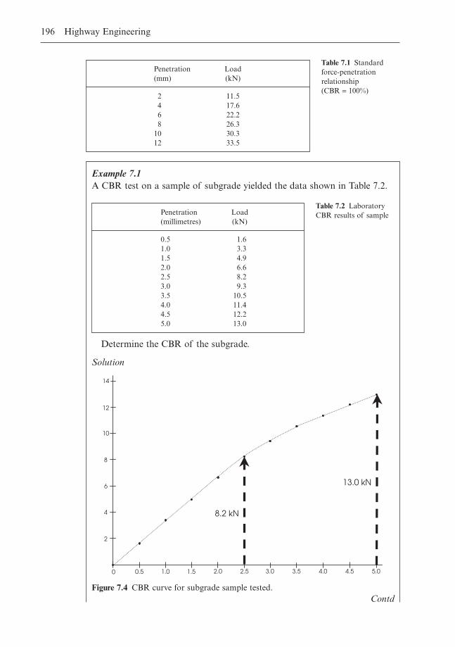
196 Highway Engineering
Penetration Load(mm) (kN)
2 11.54 17.66 22.28 26.3
10 30.312 33.5
Table 7.1 Standardforce-penetrationrelationship (CBR = 100%)
Example 7.1A CBR test on a sample of subgrade yielded the data shown in Table 7.2.
Determine the CBR of the subgrade.
Solution
Penetration Load(millimetres) (kN)
0.5 1.61.0 3.31.5 4.92.0 6.62.5 8.23.0 9.33.5 10.54.0 11.44.5 12.25.0 13.0
Table 7.2 LaboratoryCBR results of sample
2
4
6
8
10
12
14
1.0 1.5 2.0 2.5 3.0 3.5 4.0 4.5 5.0 0.50
8.2 kN
13.0 kN
Figure 7.4 CBR curve for subgrade sample tested.Contd
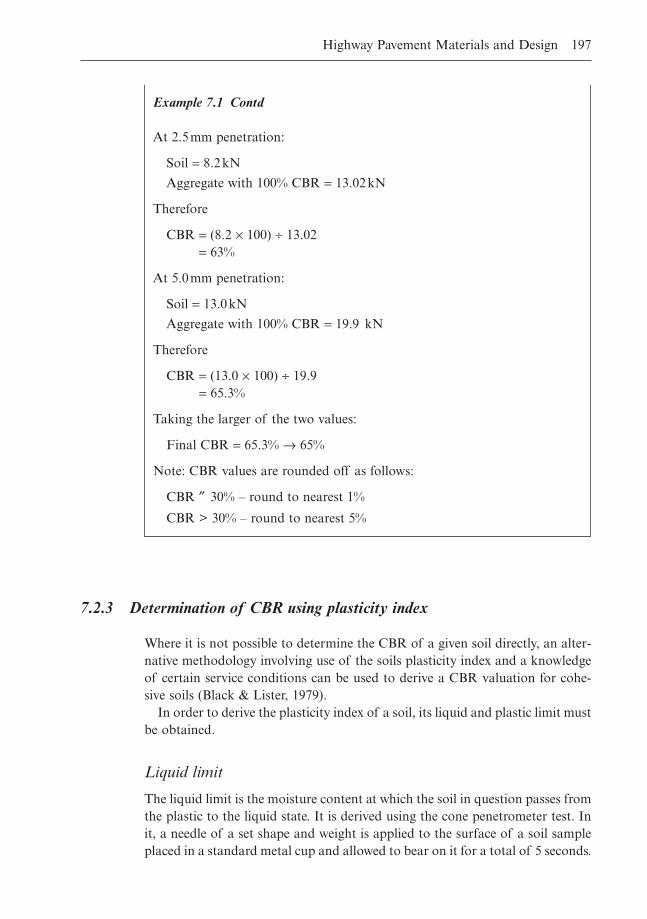
Highway Pavement Materials and Design 197
7.2.3 Determination of CBR using plasticity index
Where it is not possible to determine the CBR of a given soil directly, an alter-native methodology involving use of the soils plasticity index and a knowledgeof certain service conditions can be used to derive a CBR valuation for cohe-sive soils (Black & Lister, 1979).
In order to derive the plasticity index of a soil, its liquid and plastic limit mustbe obtained.
Liquid limit
The liquid limit is the moisture content at which the soil in question passes fromthe plastic to the liquid state. It is derived using the cone penetrometer test. Init, a needle of a set shape and weight is applied to the surface of a soil sampleplaced in a standard metal cup and allowed to bear on it for a total of 5 seconds.
Example 7.1 Contd
At 2.5mm penetration:
Soil = 8.2kN
Aggregate with 100% CBR = 13.02kN
Therefore
CBR = (8.2 ¥ 100) ∏ 13.02= 63%
At 5.0mm penetration:
Soil = 13.0kN
Aggregate with 100% CBR = 19.9 kN
Therefore
CBR = (13.0 ¥ 100) ∏ 19.9= 65.3%
Taking the larger of the two values:
Final CBR = 65.3% Æ 65%
Note: CBR values are rounded off as follows:
CBR ≤ 30% – round to nearest 1%
CBR > 30% – round to nearest 5%
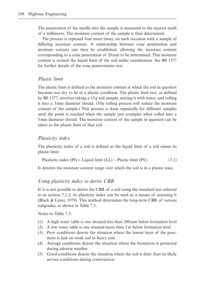
The penetration of the needle into the sample is measured to the nearest tenthof a millimetre. The moisture content of the sample is then determined.
The process is repeated four more times, on each occasion with a sample ofdiffering moisture content. A relationship between cone penetration and moisture content can then be established, allowing the moisture content corresponding to a cone penetration of 20mm to be determined. This moisturecontent is termed the liquid limit of the soil under examination. See BS 1377for further details of the cone penetrometer test.
Plastic limit
The plastic limit is defined as the moisture content at which the soil in questionbecomes too dry to be in a plastic condition. The plastic limit test, as definedby BS 1377, involves taking a 15g soil sample, mixing it with water, and rollingit into a 3mm diameter thread. (The rolling process will reduce the moisturecontent of the sample.) This process is done repeatedly for different samplesuntil the point is reached when the sample just crumples when rolled into a 3mm diameter thread. The moisture content of the sample in question can betaken as the plastic limit of that soil.
Plasticity index
The plasticity index of a soil is defined as the liquid limit of a soil minus itsplastic limit:
Plasticity index (PI) = Liquid limit (LL) - Plastic limit (PL) (7.1)
It denotes the moisture content range over which the soil is in a plastic state.
Using plasticity index to derive CBR
If it is not possible to derive the CBR of a soil using the standard test referredto in section 7.2.2, its plasticity index can be used as a means of assessing it(Black & Lister, 1979). This method determines the long-term CBR of varioussubgrades, as shown in Table 7.3.
Notes to Table 7.3:
(1) A high water table is one situated less than 300mm below formation level(2) A low water table is one situated more than 1m below formation level(3) Poor conditions denote the situation where the lowest layer of the pave-
ment is laid on weak soil in heavy rain(4) Average conditions denote the situation where the formation is protected
during adverse weather(5) Good conditions denote the situation where the soil is drier than its likely
service conditions during construction
198 Highway Engineering
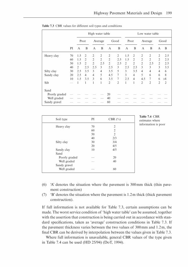
Highway Pavement Materials and Design 199
(6) ‘A’ denotes the situation where the pavement is 300mm thick (thin pave-ment construction)
(7) ‘B’ denotes the situation where the pavement is 1.2m thick (thick pavementconstruction).
If full information is not available for Table 7.3, certain assumptions can bemade. The worst service condition of ‘high water table’ can be assumed, togetherwith the assertion that construction is being carried out in accordance with stan-dard specifications, taken as ‘average’ construction conditions in Table 7.3. Ifthe pavement thickness varies between the two values of 300mm and 1.2m, thefinal CBR can be derived by interpolation between the values given in Table 7.3.
Where full information is unavailable, general CBR values of the type givenin Table 7.4 can be used (HD 25/94) (DoT, 1994).
High water table Low water table
Poor Average Good Poor Average Good
PI A B A B A B A B A B A B
Heavy clay 70 1.5 2 2 2 2 2 1.5 2 2 2 2 2.560 1.5 2 2 2 2 2.5 1.5 2 2 2 2 2.550 1.5 2 2 2.5 2 2.5 2 2 2 2.5 2 2.540 2 2.5 2.5 3 2.5 3 2.5 2.5 3 3 3 3.5
Silty clay 30 2.5 3.5 3 4 3.5 5 3 3.5 4 4 4 6Sandy clay 20 2.5 4 4 5 4.5 7 3 4 5 6 6 8
10 1.5 3.5 3 6 3.5 7 2.5 4 4.5 7 6 >8Silt — 1 1 1 1 2 2 1 1 2 2 2 2
SandPoorly graded — — — — — 20 — — — — — — —Well graded — — — — — 40 — — — — — — —
Sandy gravel — — — — — 60 — — — — — — —
Table 7.3 CBR values for different soil types and conditions
Soil type PI CBR (%)
Heavy clay 70 260 250 240 2/3
Silty clay 30 3/420 4/5
Sandy clay 10 4/5Sand
Poorly graded — 20Well graded — 40
Sandy gravelWell graded — 60
Table 7.4 CBRestimates whereinformation is poor
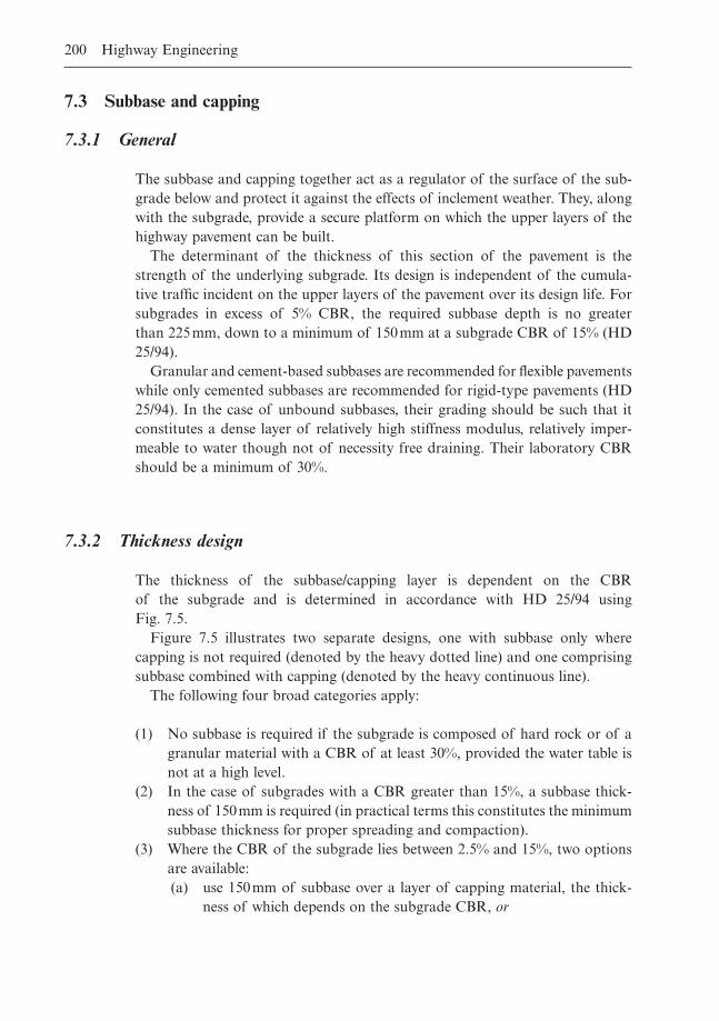
200 Highway Engineering
7.3 Subbase and capping
7.3.1 General
The subbase and capping together act as a regulator of the surface of the sub-grade below and protect it against the effects of inclement weather. They, alongwith the subgrade, provide a secure platform on which the upper layers of thehighway pavement can be built.
The determinant of the thickness of this section of the pavement is thestrength of the underlying subgrade. Its design is independent of the cumula-tive traffic incident on the upper layers of the pavement over its design life. Forsubgrades in excess of 5% CBR, the required subbase depth is no greater than 225mm, down to a minimum of 150mm at a subgrade CBR of 15% (HD25/94).
Granular and cement-based subbases are recommended for flexible pavementswhile only cemented subbases are recommended for rigid-type pavements (HD25/94). In the case of unbound subbases, their grading should be such that itconstitutes a dense layer of relatively high stiffness modulus, relatively imper-meable to water though not of necessity free draining. Their laboratory CBRshould be a minimum of 30%.
7.3.2 Thickness design
The thickness of the subbase/capping layer is dependent on the CBR of the subgrade and is determined in accordance with HD 25/94 using Fig. 7.5.
Figure 7.5 illustrates two separate designs, one with subbase only wherecapping is not required (denoted by the heavy dotted line) and one comprisingsubbase combined with capping (denoted by the heavy continuous line).
The following four broad categories apply:
(1) No subbase is required if the subgrade is composed of hard rock or of agranular material with a CBR of at least 30%, provided the water table isnot at a high level.
(2) In the case of subgrades with a CBR greater than 15%, a subbase thick-ness of 150mm is required (in practical terms this constitutes the minimumsubbase thickness for proper spreading and compaction).
(3) Where the CBR of the subgrade lies between 2.5% and 15%, two optionsare available:(a) use 150mm of subbase over a layer of capping material, the thick-
ness of which depends on the subgrade CBR, or
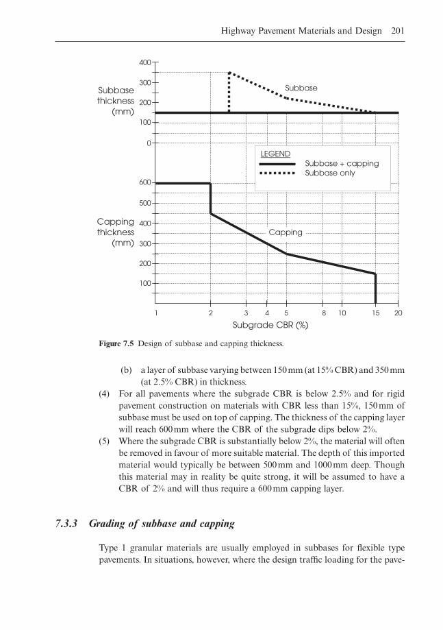
Highway Pavement Materials and Design 201
(b) a layer of subbase varying between 150mm (at 15% CBR) and 350mm(at 2.5% CBR) in thickness.
(4) For all pavements where the subgrade CBR is below 2.5% and for rigidpavement construction on materials with CBR less than 15%, 150mm ofsubbase must be used on top of capping. The thickness of the capping layerwill reach 600mm where the CBR of the subgrade dips below 2%.
(5) Where the subgrade CBR is substantially below 2%, the material will oftenbe removed in favour of more suitable material. The depth of this importedmaterial would typically be between 500mm and 1000mm deep. Thoughthis material may in reality be quite strong, it will be assumed to have aCBR of 2% and will thus require a 600mm capping layer.
7.3.3 Grading of subbase and capping
Type 1 granular materials are usually employed in subbases for flexible typepavements. In situations, however, where the design traffic loading for the pave-
Subbase
400
300
200
100
0
600
500
400
300
200
100
2 1 3 4 5 8 10 15 20
Subgrade CBR (%)
Capping thickness
(mm)
Subbasethickness
(mm)
LEGEND Subbase + capping Subbase only
Capping
Figure 7.5 Design of subbase and capping thickness.
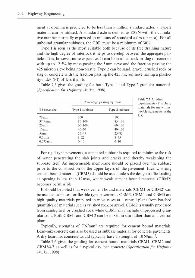
202 Highway Engineering
ment at opening is predicted to be less than 5 million standard axles, a Type 2material can be utilised. A standard axle is defined as 80kN with the cumula-tive number normally expressed in millions of standard axles (or msa). For allunbound granular subbases, the CBR must be a minimum of 30%.
Type 1 is seen as the most suitable both because of its free draining natureand the high degree of interlock it helps to develop between the aggregate par-ticles. It is, however, more expensive. It can be crushed rock or slag or concretewith up to 12.5% by mass passing the 5mm sieve and the fraction passing the425 micron sieve being non-plastic. Type 2 can be sand, gravel, crushed rock orslag or concrete with the fraction passing the 425 micron sieve having a plastic-ity index (PI) of less than 6.
Table 7.5 gives the grading for both Type 1 and Type 2 granular materials(Specification for Highway Works, 1998).
Percentage passing by mass
BS sieve size Type 1 subbase Type 2 subbase
75mm 100 10037.5mm 85–100 85–10020mm 60–100 60–10010mm 40–70 40–1005mm 25–45 25–850.6mm 8–22 8–450.075mm 0–10 0–10
Table 7.5 Gradingrequirements of subbasematerials for use withinflexible pavements in theUK
For rigid-type pavements, a cemented subbase is required to minimise the riskof water penetrating the slab joints and cracks and thereby weakening thesubbase itself. An impermeable membrane should be placed over the subbaseprior to the construction of the upper layers of the pavement. Ideally, strongcement bound material (CBM3) should be used, unless the design traffic loadingat opening is less than 12msa, where weak cement bound material (CBM2)becomes permissible.
It should be noted that weak cement bound materials (CBM1 or CBM2) canbe used as subbases for flexible type pavements. CBM3, CBM4 and CBM5 arehigh quality materials prepared in most cases at a central plant from batchedquantities of material such as crushed rock or gravel. CBM2 is usually processedfrom sand/gravel or crushed rock while CBM1 may include unprocessed gran-ular soils. Both CBM1 and CBM 2 can be mixed in situ rather than at a centralplant.
Typically, strengths of 7N/mm2 are required for cement bound materials.Lean-mix concrete can also be used as subbase material for concrete pavements.A dry lean-mix concrete would typically have a strength of 10N/mm2.
Table 7.6 gives the grading for cement bound materials CBM1, CBM2 andCBM3/4/5 as well as for a typical dry lean concrete (Specification for HighwayWorks, 1998)
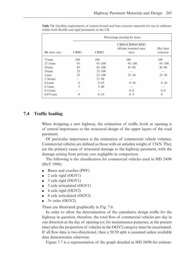
Highway Pavement Materials and Design 203
7.4 Traffic loading
When designing a new highway, the estimation of traffic levels at opening is of central importance to the structural design of the upper layers of the roadpavement.
Of particular importance is the estimation of commercial vehicle volumes.Commercial vehicles are defined as those with an unladen weight of 15kN. Theyare the primary cause of structural damage to the highway pavement, with thedamage arising from private cars negligible in comparison.
The following is the classification for commercial vehicles used in HD 24/96(DoT 1996):
� Buses and coaches (PSV)� 2 axle rigid (OGV1)� 3 axle rigid (OGV1)� 3 axle articulated (OGV1)� 4 axle rigid (OGV2)� 4 axle articulated (OGV2)� 5+ axles (OGV2).
These are illustrated graphically in Fig. 7.6.In order to allow the determination of the cumulative design traffic for the
highway in question, therefore, the total flow of commercial vehicles per day inone direction at the day of opening (or, for maintenance purposes, at the presenttime) plus the proportion of vehicles in the OGV2 category must be ascertained.If all flow data is two-directional, then a 50:50 split is assumed unless availabledata demonstrates otherwise.
Figure 7.7 is a representation of the graph detailed in HD 24/96 for estimat-
Percentage passing by mass
CBM3/CBM4/CBM5(40mm nominal max Dry lean
BS sieve size CBM1 CBM2 size) concrete
75mm 100 100 100 10037.5mm 95 95–100 95–100 95–10020mm 45 45–100 45–80 45–8010mm 35 35–100 — —5mm 25 25–100 25–50 25–502.36mm — 15–90 — —0.6mm 8 8–65 8–30 8–300.3mm 5 5–40 — —0.15mm — — 0–8 0–80.075mm 0 0–10 0–5 0
Table 7.6 Grading requirements of cement-bound and lean concrete materials for use in subbaseswithin both flexible and rigid pavements in the UK
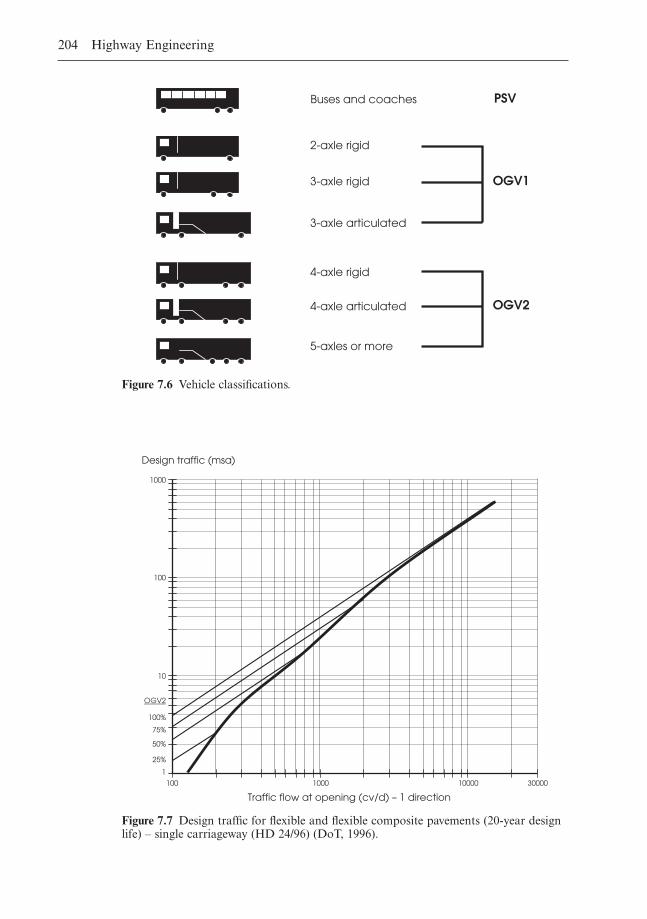
204 Highway Engineering
Buses and coaches
2-axle rigid
3-axle rigid
3-axle articulated
4-axle rigid
4-axle articulated
5-axles or more
PSV
OGV1
OGV2
Figure 7.6 Vehicle classifications.
Traffic flow at opening (cv/d) – 1 direction
100 1000 10000 30000
1
10
100
1000
Design traffic (msa)
75%
50%
25%
100%
OGV2
Figure 7.7 Design traffic for flexible and flexible composite pavements (20-year designlife) – single carriageway (HD 24/96) (DoT, 1996).
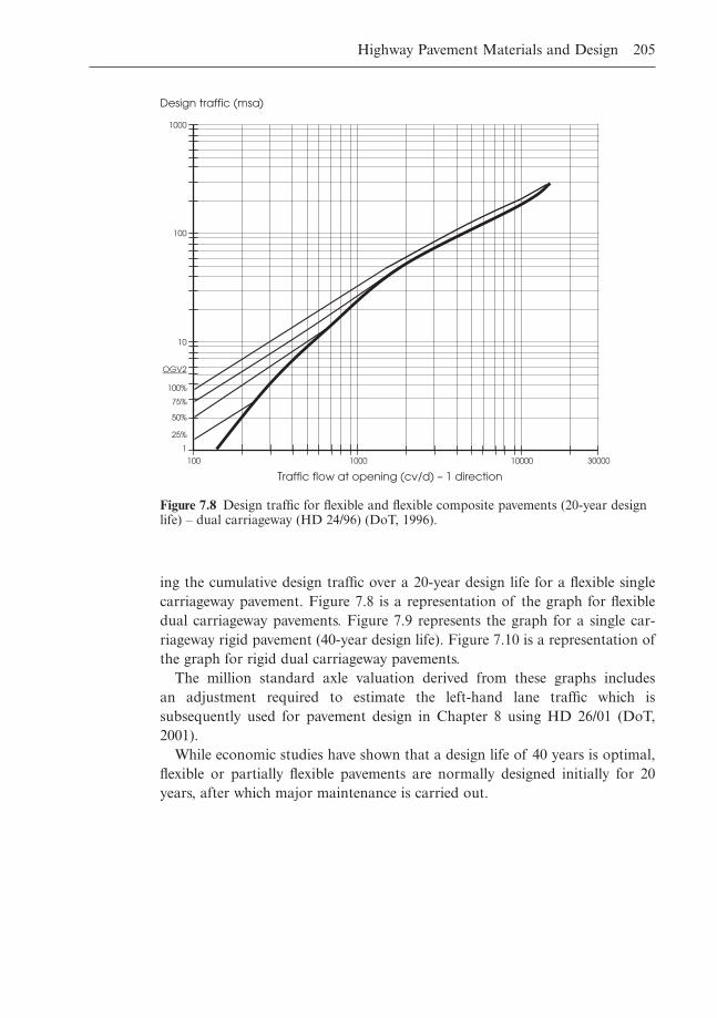
Highway Pavement Materials and Design 205
Traffic flow at opening (cv/d) – 1 direction
100 1000 10000 30000
1
10
100
1000
Design traffic (msa)
75%
50%
25%
100%
OGV2
Figure 7.8 Design traffic for flexible and flexible composite pavements (20-year designlife) – dual carriageway (HD 24/96) (DoT, 1996).
ing the cumulative design traffic over a 20-year design life for a flexible singlecarriageway pavement. Figure 7.8 is a representation of the graph for flexibledual carriageway pavements. Figure 7.9 represents the graph for a single car-riageway rigid pavement (40-year design life). Figure 7.10 is a representation ofthe graph for rigid dual carriageway pavements.
The million standard axle valuation derived from these graphs includes an adjustment required to estimate the left-hand lane traffic which is subsequently used for pavement design in Chapter 8 using HD 26/01 (DoT,2001).
While economic studies have shown that a design life of 40 years is optimal,flexible or partially flexible pavements are normally designed initially for 20years, after which major maintenance is carried out.
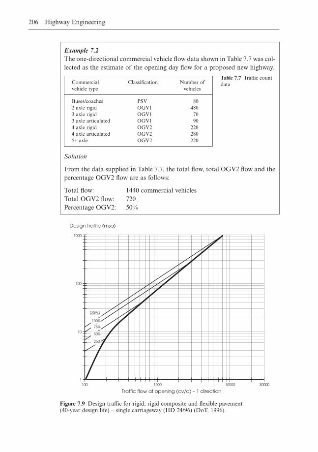
206 Highway Engineering
Example 7.2The one-directional commercial vehicle flow data shown in Table 7.7 was col-lected as the estimate of the opening day flow for a proposed new highway.
Solution
From the data supplied in Table 7.7, the total flow, total OGV2 flow and thepercentage OGV2 flow are as follows:
Total flow: 1440 commercial vehiclesTotal OGV2 flow: 720Percentage OGV2: 50%
Commercial Classification Number ofvehicle type vehicles
Buses/coaches PSV 802 axle rigid OGV1 4803 axle rigid OGV1 703 axle articulated OGV1 904 axle rigid OGV2 2204 axle articulated OGV2 2805+ axle OGV2 220
Table 7.7 Traffic countdata
Traffic flow at opening (cv/d) – 1 direction100 1000 10000 30000
1
10
100
1000
Design traffic (msa)
75%
50%
25%
100%
OGV2
Figure 7.9 Design traffic for rigid, rigid composite and flexible pavement (40-year design life) – single carriageway (HD 24/96) (DoT, 1996).
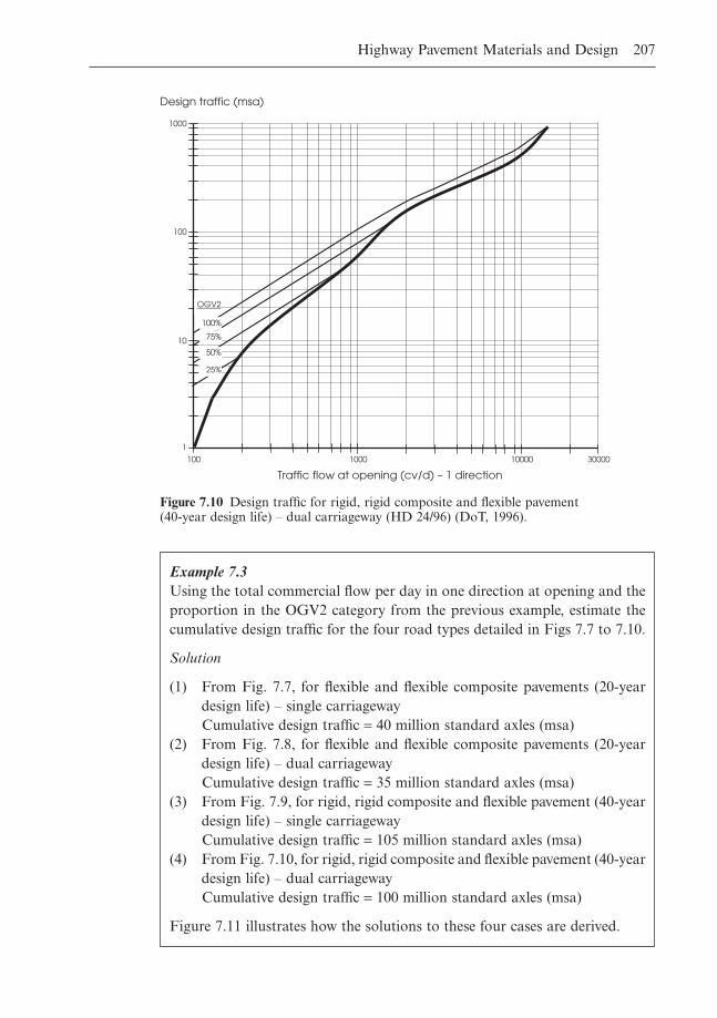
Highway Pavement Materials and Design 207
Example 7.3Using the total commercial flow per day in one direction at opening and theproportion in the OGV2 category from the previous example, estimate thecumulative design traffic for the four road types detailed in Figs 7.7 to 7.10.
Solution
(1) From Fig. 7.7, for flexible and flexible composite pavements (20-yeardesign life) – single carriagewayCumulative design traffic = 40 million standard axles (msa)
(2) From Fig. 7.8, for flexible and flexible composite pavements (20-yeardesign life) – dual carriagewayCumulative design traffic = 35 million standard axles (msa)
(3) From Fig. 7.9, for rigid, rigid composite and flexible pavement (40-yeardesign life) – single carriagewayCumulative design traffic = 105 million standard axles (msa)
(4) From Fig. 7.10, for rigid, rigid composite and flexible pavement (40-yeardesign life) – dual carriagewayCumulative design traffic = 100 million standard axles (msa)
Figure 7.11 illustrates how the solutions to these four cases are derived.
Traffic flow at opening (cv/d) – 1 direction
100 1000 10000 30000
1
10
100
1000
Design traffic (msa)
75%
50%
25%
100%
OGV2
Figure 7.10 Design traffic for rigid, rigid composite and flexible pavement (40-year design life) – dual carriageway (HD 24/96) (DoT, 1996).
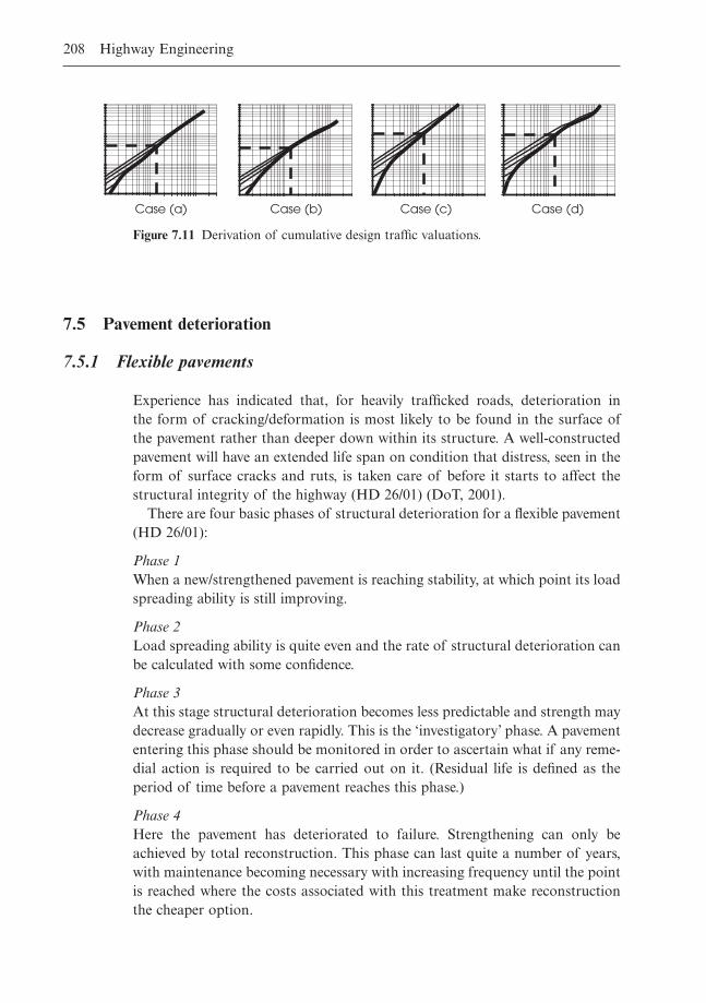
208 Highway Engineering
Case (a) Case (b) Case (c) Case (d)
Figure 7.11 Derivation of cumulative design traffic valuations.
7.5 Pavement deterioration
7.5.1 Flexible pavements
Experience has indicated that, for heavily trafficked roads, deterioration in the form of cracking/deformation is most likely to be found in the surface ofthe pavement rather than deeper down within its structure. A well-constructedpavement will have an extended life span on condition that distress, seen in theform of surface cracks and ruts, is taken care of before it starts to affect thestructural integrity of the highway (HD 26/01) (DoT, 2001).
There are four basic phases of structural deterioration for a flexible pavement(HD 26/01):
Phase 1When a new/strengthened pavement is reaching stability, at which point its loadspreading ability is still improving.
Phase 2Load spreading ability is quite even and the rate of structural deterioration canbe calculated with some confidence.
Phase 3At this stage structural deterioration becomes less predictable and strength maydecrease gradually or even rapidly. This is the ‘investigatory’ phase. A pavemententering this phase should be monitored in order to ascertain what if any reme-dial action is required to be carried out on it. (Residual life is defined as theperiod of time before a pavement reaches this phase.)
Phase 4Here the pavement has deteriorated to failure. Strengthening can only beachieved by total reconstruction. This phase can last quite a number of years,with maintenance becoming necessary with increasing frequency until the pointis reached where the costs associated with this treatment make reconstructionthe cheaper option.
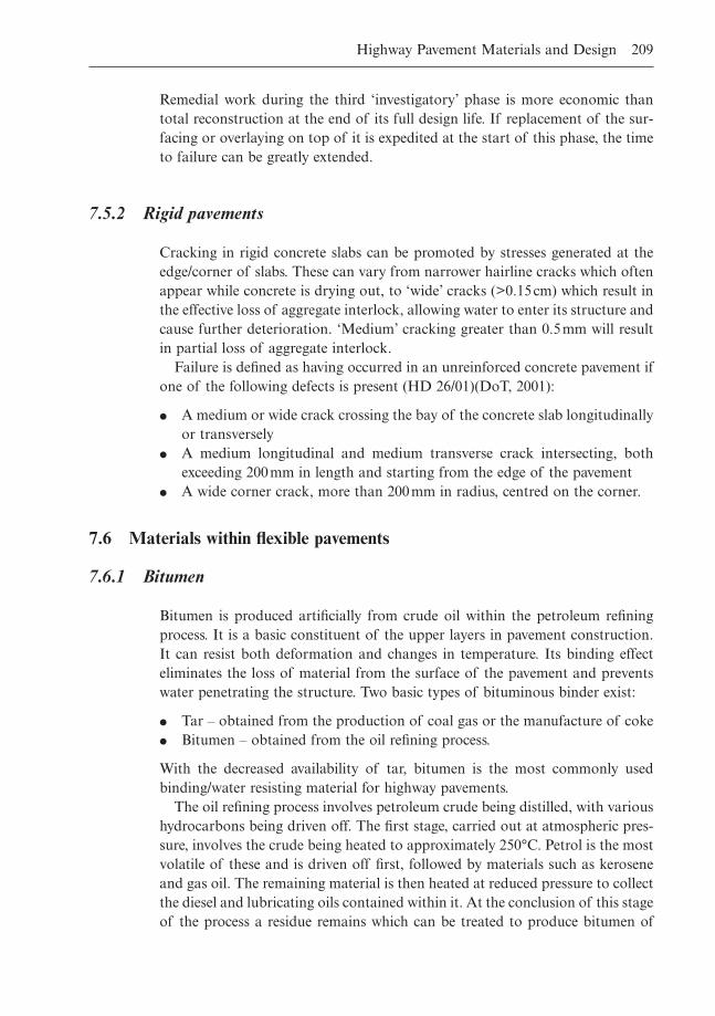
Remedial work during the third ‘investigatory’ phase is more economic thantotal reconstruction at the end of its full design life. If replacement of the sur-facing or overlaying on top of it is expedited at the start of this phase, the timeto failure can be greatly extended.
7.5.2 Rigid pavements
Cracking in rigid concrete slabs can be promoted by stresses generated at theedge/corner of slabs. These can vary from narrower hairline cracks which oftenappear while concrete is drying out, to ‘wide’ cracks (>0.15cm) which result inthe effective loss of aggregate interlock, allowing water to enter its structure andcause further deterioration. ‘Medium’ cracking greater than 0.5mm will resultin partial loss of aggregate interlock.
Failure is defined as having occurred in an unreinforced concrete pavement ifone of the following defects is present (HD 26/01)(DoT, 2001):
� A medium or wide crack crossing the bay of the concrete slab longitudinallyor transversely
� A medium longitudinal and medium transverse crack intersecting, bothexceeding 200mm in length and starting from the edge of the pavement
� A wide corner crack, more than 200mm in radius, centred on the corner.
7.6 Materials within flexible pavements
7.6.1 Bitumen
Bitumen is produced artificially from crude oil within the petroleum refiningprocess. It is a basic constituent of the upper layers in pavement construction.It can resist both deformation and changes in temperature. Its binding effecteliminates the loss of material from the surface of the pavement and preventswater penetrating the structure. Two basic types of bituminous binder exist:
� Tar – obtained from the production of coal gas or the manufacture of coke� Bitumen – obtained from the oil refining process.
With the decreased availability of tar, bitumen is the most commonly usedbinding/water resisting material for highway pavements.
The oil refining process involves petroleum crude being distilled, with varioushydrocarbons being driven off. The first stage, carried out at atmospheric pres-sure, involves the crude being heated to approximately 250°C. Petrol is the mostvolatile of these and is driven off first, followed by materials such as keroseneand gas oil. The remaining material is then heated at reduced pressure to collectthe diesel and lubricating oils contained within it. At the conclusion of this stageof the process a residue remains which can be treated to produce bitumen of
Highway Pavement Materials and Design 209
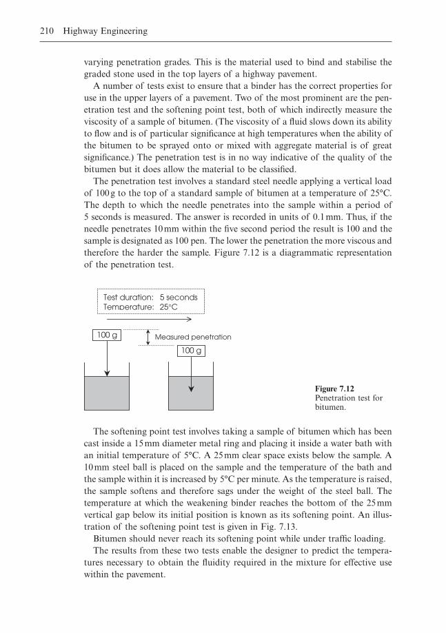
210 Highway Engineering
varying penetration grades. This is the material used to bind and stabilise thegraded stone used in the top layers of a highway pavement.
A number of tests exist to ensure that a binder has the correct properties foruse in the upper layers of a pavement. Two of the most prominent are the pen-etration test and the softening point test, both of which indirectly measure theviscosity of a sample of bitumen. (The viscosity of a fluid slows down its abilityto flow and is of particular significance at high temperatures when the ability ofthe bitumen to be sprayed onto or mixed with aggregate material is of great significance.) The penetration test is in no way indicative of the quality of thebitumen but it does allow the material to be classified.
The penetration test involves a standard steel needle applying a vertical loadof 100g to the top of a standard sample of bitumen at a temperature of 25°C.The depth to which the needle penetrates into the sample within a period of5 seconds is measured. The answer is recorded in units of 0.1mm. Thus, if theneedle penetrates 10mm within the five second period the result is 100 and thesample is designated as 100 pen. The lower the penetration the more viscous andtherefore the harder the sample. Figure 7.12 is a diagrammatic representationof the penetration test.
100 g
100 g
Measured penetration
Test duration: 5 secondsTemperature: 25∞C
Figure 7.12Penetration test forbitumen.
The softening point test involves taking a sample of bitumen which has beencast inside a 15mm diameter metal ring and placing it inside a water bath withan initial temperature of 5°C. A 25mm clear space exists below the sample. A10mm steel ball is placed on the sample and the temperature of the bath andthe sample within it is increased by 5°C per minute. As the temperature is raised,the sample softens and therefore sags under the weight of the steel ball. Thetemperature at which the weakening binder reaches the bottom of the 25mmvertical gap below its initial position is known as its softening point. An illus-tration of the softening point test is given in Fig. 7.13.
Bitumen should never reach its softening point while under traffic loading.The results from these two tests enable the designer to predict the tempera-
tures necessary to obtain the fluidity required in the mixture for effective usewithin the pavement.
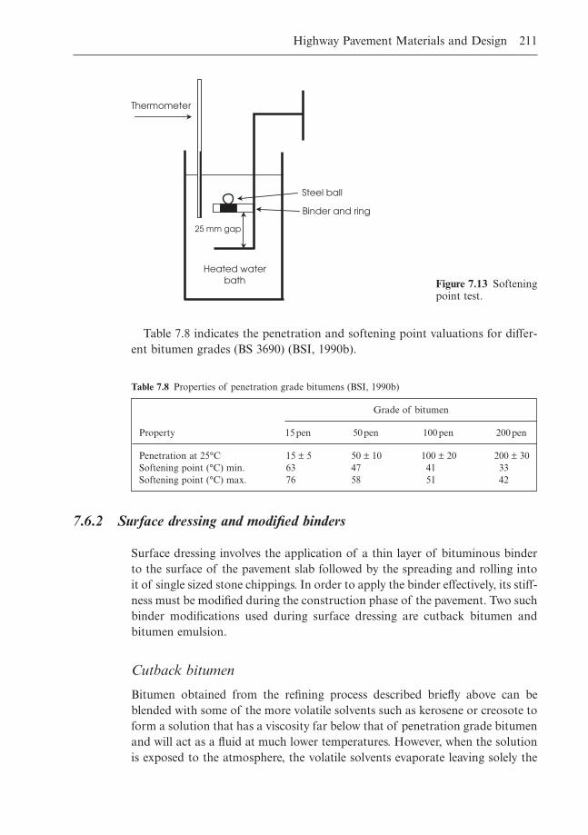
Highway Pavement Materials and Design 211
Table 7.8 indicates the penetration and softening point valuations for differ-ent bitumen grades (BS 3690) (BSI, 1990b).
Heated water bath
25 mm gap
Steel ball
Binder and ring
Thermometer
Figure 7.13 Softeningpoint test.
Grade of bitumen
Property 15pen 50pen 100pen 200pen
Penetration at 25°C 15 ± 5 50 ± 10 100 ± 20 200 ± 30Softening point (°C) min. 63 47 41 33Softening point (°C) max. 76 58 51 42
Table 7.8 Properties of penetration grade bitumens (BSI, 1990b)
7.6.2 Surface dressing and modified binders
Surface dressing involves the application of a thin layer of bituminous binderto the surface of the pavement slab followed by the spreading and rolling intoit of single sized stone chippings. In order to apply the binder effectively, its stiff-ness must be modified during the construction phase of the pavement. Two suchbinder modifications used during surface dressing are cutback bitumen andbitumen emulsion.
Cutback bitumen
Bitumen obtained from the refining process described briefly above can beblended with some of the more volatile solvents such as kerosene or creosote toform a solution that has a viscosity far below that of penetration grade bitumenand will act as a fluid at much lower temperatures. However, when the solutionis exposed to the atmosphere, the volatile solvents evaporate leaving solely the
bitumen in place. Such solutions are termed cutbacks and the process of evap-oration of the volatile solvents is called curing. The speed at which it occurs willdepend on the nature of the solvent.
The classification of cutbacks is based on the following two characteristics:
� The viscosity of the cutback itself� The penetration of the non-volatile residue.
The cutback’s viscosity is measured using a standard tar viscometer (STV) whichcomputes the time in seconds for a given volume of binder to flow through astandard orifice at a temperature of 40°C. Three common grades for cutbackhave viscosities of 50, 100 and 200 seconds. Cutback bitumen is used in surfacedressing. In this process, it is sprayed onto a weakened road surface and chip-pings are placed on it and then rolled. It serves to provide a non-skid wearingsurface to the pavement, makes the surface resistant to water and prevents itsdisintegration.
Bituminous emulsions
Bitumen can be made easier to handle by forming it into an emulsion whereparticles of it become suspended in water. In most cases, their manufactureinvolves heating the bitumen and then shredding it in a colloidal mill with asolution of hot water and an emulsifier. The particles are imparted with an ioniccharge which makes them repel each other. Within cationic emulsions theimparted charge is positive, while the charge is negative in anionic emulsions.When the emulsion is sprayed onto the road surface, the charged ions areattracted to opposite charges on the surface, causing the emulsion to begin‘breaking’ with the bitumen particles starting to coalesce together. The break-ing process is complete when the film of bitumen is continuous.
Bitumen emulsions are graded in terms of their stability or rate of break ona scale of 1 to 4, with 1 signifying the greatest stability (stable = rapid acting).Rate of break depends on the composition of the emulsion and the rate at whichthe emulsion evaporates. The grading of the aggregate onto which the emulsionis applied is also important to the rate of break. Dirty aggregates accelerate it,as will porous or dry road surfaces. Cationic emulsions tend to break morerapidly than ionic ones. The UK code, BS 434 (BSI, 1984), also designatescationic emulsions as K and ionic as A. Therefore, K3 denotes a slow actingcationic emulsion, K2 a medium acting one and K1 a rapid acting one.
Chippings
The chippings used are central to the success of the surface dressing process asthey provide essential skidding resistance. The correct rate of spread dependsmainly on the nominal size of chippings used, varying from 7kg per m2 for 6mm nominal size to 17kg per m2 for 20mm. The chippings themselves may be
212 Highway Engineering
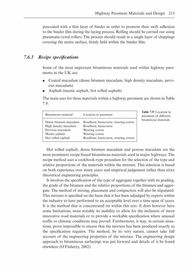
Highway Pavement Materials and Design 213
precoated with a thin layer of binder in order to promote their swift adhesionto the binder film during the laying process. Rolling should be carried out usingpneumatic-tyred rollers. The process should result in a single layer of chippingscovering the entire surface, firmly held within the binder film.
7.6.3 Recipe specifications
Some of the most important bituminous materials used within highway pave-ments in the UK are:
� Coated macadam (dense bitumen macadam, high density macadam, pervi-ous macadam)
� Asphalt (mastic asphalt, hot rolled asphalt).
The main uses for these materials within a highway pavement are shown in Table7.9.
Bituminous material Location in pavement
Dense bitumen macadam Roadbase, basecourse, wearing courseHigh density macadam Roadbase, basecoursePervious macadam Wearing courseMastic asphalt Wearing courseHot rolled asphalt Roadbase, basecourse, wearing course
Table 7.9 Location inpavement of differentbituminous materials
Hot rolled asphalt, dense bitumen macadam and porous macadam are themost prominent recipe-based bituminous materials used in major highways. Therecipe method uses a cookbook-type procedure for the selection of the type andrelative proportions of the materials within the mixture. This selection is basedon both experience over many years and empirical judgement rather than stricttheoretical engineering principles.
It involves the specification of the type of aggregate together with its grading,the grade of the bitumen and the relative proportions of the bitumen and aggre-gate. The method of mixing, placement and compaction will also be stipulated.This mixture is specified on the basis that it has been adjudged by experts withinthe industry to have performed to an acceptable level over a time span of years.It is the method that is concentrated on within this text. It does however havesome limitations, most notably its inability to allow for the inclusion of moreinnovative road materials or to provide a workable specification where unusualtraffic or climatic conditions may prevail. Furthermore, it may, in certain situa-tions, prove impossible to ensure that the mixture has been produced exactly asthe specification requires. The method, by its very nature, cannot take fullaccount of the engineering properties of the mixture. The engineering designapproach to bituminous surfacings was put forward and details of it be foundelsewhere (O’Flaherty, 2002).
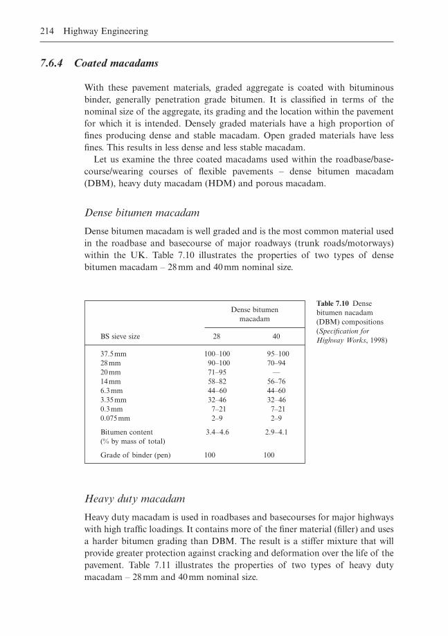
214 Highway Engineering
7.6.4 Coated macadams
With these pavement materials, graded aggregate is coated with bituminousbinder, generally penetration grade bitumen. It is classified in terms of thenominal size of the aggregate, its grading and the location within the pavementfor which it is intended. Densely graded materials have a high proportion offines producing dense and stable macadam. Open graded materials have lessfines. This results in less dense and less stable macadam.
Let us examine the three coated macadams used within the roadbase/base-course/wearing courses of flexible pavements – dense bitumen macadam(DBM), heavy duty macadam (HDM) and porous macadam.
Dense bitumen macadam
Dense bitumen macadam is well graded and is the most common material usedin the roadbase and basecourse of major roadways (trunk roads/motorways)within the UK. Table 7.10 illustrates the properties of two types of densebitumen macadam – 28mm and 40mm nominal size.
Dense bitumenmacadam
BS sieve size 28 40
37.5mm 100–100 95–10028mm 90–100 70–9420mm 71–95 —14mm 58–82 56–766.3mm 44–60 44–603.35mm 32–46 32–460.3mm 7–21 7–210.075mm 2–9 2–9
Bitumen content 3.4–4.6 2.9–4.1(% by mass of total)
Grade of binder (pen) 100 100
Table 7.10 Densebitumen nacadam(DBM) compositions(Specification forHighway Works, 1998)
Heavy duty macadam
Heavy duty macadam is used in roadbases and basecourses for major highwayswith high traffic loadings. It contains more of the finer material (filler) and usesa harder bitumen grading than DBM. The result is a stiffer mixture that willprovide greater protection against cracking and deformation over the life of thepavement. Table 7.11 illustrates the properties of two types of heavy dutymacadam – 28mm and 40mm nominal size.
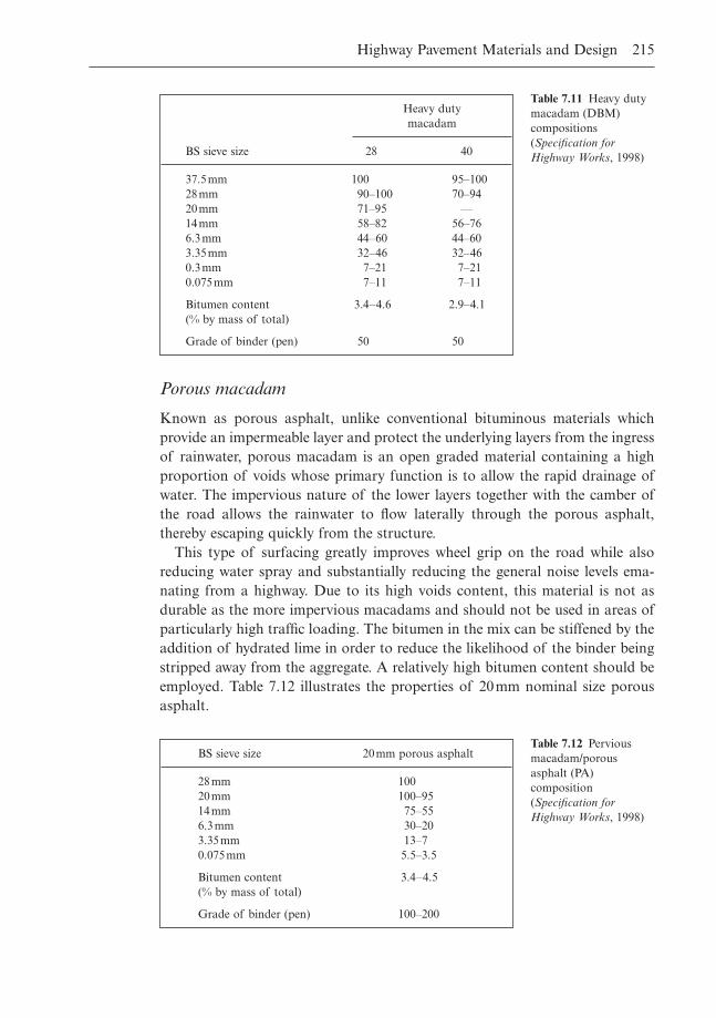
Highway Pavement Materials and Design 215
Porous macadam
Known as porous asphalt, unlike conventional bituminous materials whichprovide an impermeable layer and protect the underlying layers from the ingressof rainwater, porous macadam is an open graded material containing a highproportion of voids whose primary function is to allow the rapid drainage ofwater. The impervious nature of the lower layers together with the camber ofthe road allows the rainwater to flow laterally through the porous asphalt,thereby escaping quickly from the structure.
This type of surfacing greatly improves wheel grip on the road while alsoreducing water spray and substantially reducing the general noise levels ema-nating from a highway. Due to its high voids content, this material is not asdurable as the more impervious macadams and should not be used in areas ofparticularly high traffic loading. The bitumen in the mix can be stiffened by theaddition of hydrated lime in order to reduce the likelihood of the binder beingstripped away from the aggregate. A relatively high bitumen content should beemployed. Table 7.12 illustrates the properties of 20mm nominal size porousasphalt.
Heavy duty macadam
BS sieve size 28 40
37.5mm 100 95–10028mm 90–100 70–9420mm 71–95 —14mm 58–82 56–766.3mm 44–60 44–603.35mm 32–46 32–460.3mm 7–21 7–210.075mm 7–11 7–11
Bitumen content 3.4–4.6 2.9–4.1(% by mass of total)
Grade of binder (pen) 50 50
Table 7.11 Heavy dutymacadam (DBM)compositions(Specification forHighway Works, 1998)
BS sieve size 20mm porous asphalt
28mm 10020mm 100–9514mm 75–556.3mm 30–203.35mm 13–70.075mm 5.5–3.5
Bitumen content 3.4–4.5(% by mass of total)
Grade of binder (pen) 100–200
Table 7.12 Perviousmacadam/porousasphalt (PA)composition(Specification forHighway Works, 1998)
7.6.5 Asphalts
Two asphalts are discussed within this section: hot rolled asphalt (HRA) andmastic asphalt.
Hot rolled asphalt
Hot rolled asphalt is similar to a coated macadam. It is a dense material withlow air voids content, consisting of a mixture of aggregate, fines, binder and afiller material, but in this case the grading is far less continuous (gap-graded)with a higher proportion of both fines and binder present in the mix. The mate-rial is practically impervious to water, with the fines, filler and bitumen forminga mortar in which coarse aggregate is scattered in order to increase its overallbulk.
Hot rolled asphalt wearing courses typically have from zero to 55% coarseaggregate content, with basecourses having either 50% or 60% and roadbasesnormally at 60%.
There are two recipe mixes for gap-graded rolled asphalt wearing course: TypeF, characterised by the use of sand fines, and Type C, characterised by the useof crushed rock or slag fines. F denotes a finer grading of the fine aggregate withC denoting a coarser grading of the fine aggregate.
Table 7.13 details a range of mixes for hot rolled asphalt to be used at road-base, basecourse and wearing course levels within the pavement. Each mix hasa designation composed of two numbers, with the first relating to the percent-age coarse aggregate content in the mix and the second to the nominal coarseaggregate size. (The wearing courses in Table 7.13 are both Type F.)
As hot rolled asphalt wearing course is a smooth-textured material, precoatedchippings should be spread over and rolled into its surface while plastic in orderto increase skid resistance.
Mastic asphalt
Mastic asphalt is a very durable heavy-duty, weather-proof wearing course material. It consists of a mixture of asphaltic cement (low-penetration gradebitumen), fine aggregate and filler in proportions which result in a low-voidimpermeable mass. It contains a low percentage of coarse aggregate, all of whichmust pass the 14mm sieve and be retained on the 10mm sieve. The mix consistsof a high percentage of fine aggregate, with no less than 45% and no more than55% passing the 0.075mm sieve and at least 97% passing the 2.36mm sieve inaddition to high proportions of both filler material and binder. The grade ofthe binder is very high (10 to 25 pen) with less than 1% voids in the mix.
The mix is applied manually using wooden floats, at a temperature of between175°C and 225°C approximately. It requires considerable working, with the fin-ished layer measuring between 40mm and 50mm. Its low skidding resistance
216 Highway Engineering
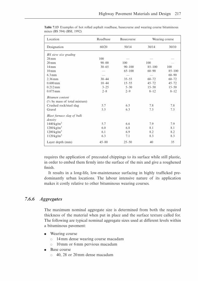
Highway Pavement Materials and Design 217
requires the application of precoated chippings to its surface while still plastic,in order to embed them firmly into the surface of the mix and give a roughenedfinish.
It results in a long-life, low-maintenance surfacing in highly trafficked pre-dominantly urban locations. The labour intensive nature of its applicationmakes it costly relative to other bituminous wearing courses.
7.6.6 Aggregates
The maximum nominal aggregate size is determined from both the requiredthickness of the material when put in place and the surface texture called for.The following are typical nominal aggregate sizes used at different levels withina bituminous pavement:
� Wearing course� 14mm dense wearing course macadam� 10mm or 6mm pervious macadam
� Base course� 40, 28 or 20mm dense macadam
Location Roadbase Basecourse Wearing course
Designation 60/20 50/14 30/14 30/10
BS sieve size grading28mm 100 — — —20mm 90–00 100 100 —14mm 30–65 90–100 85–100 10010mm — 65–100 60–90 85–1006.3mm — — — 60–902.36mm 30–44 35–55 60–72 60–720.600mm 10–44 15–55 45–72 45–720.212mm 3–25 5–30 15–50 15–500.075mm 2–8 2–9 8–12 8–12
Bitumen content(% by mass of total mixture)Crushed rock/steel slag 5.7 6.5 7.8 7.8Gravel 5.5 6.3 7.5 7.5
Blast furnace slag of bulkdensity1440kg/m3 5.7 6.6 7.9 7.91280kg/m3 6.0 6.8 8.1 8.11200kg/m3 6.1 6.9 8.2 8.21120kg/m3 6.3 7.1 8.3 8.3
Layer depth (mm) 45–80 25–50 40 35
Table 7.13 Examples of hot rolled asphalt roadbase, basecourse and wearing course bituminousmixes (BS 594) (BSI, 1992)
� Roadbase� 40 or 28mm dense macadam.
The size of aggregate must not be greater than the required layer thickness. Thelayer thickness should be approximately 21/2 times the nominal maximum aggre-gate size, with a minimum layer thickness of 11/2 times the nominal maximumaggregate size in order to minimise the likelihood of the larger stones beingcrushed during rolling.
7.6.7 Construction of bituminous road surfacings
The production of a successful bituminous road surfacing depends not just onthe design of the individual constituent layers but also on the correctness of theconstruction procedure employed to put them in place. In essence, the con-struction of a bituminous pavement consists of the flowing steps:
� Transporting and placing the bituminous material
� Compaction of the mixture
� If required, the spreading and rolling of coated chippings into the surfaceof the material.
Transporting and placing
The bituminous material is manufactured at a central batching plant where, afterthe mixing of its constituents, the material is discharged into a truck or trailerfor transportation to its final destination. The transporters must have metallicbeds sprayed with an appropriate material to prevent the mixture sticking to it.The vehicle should be designed to avoid heat loss which may result in a decreasein temperature of the material, leading to difficulties in its subsequent place-ment – if it is too cold it may prove impossible to compact properly.
It is very important that the receiving surface is clean and free of any foreignmaterials. It must, therefore, be swept clean of all loose dirt. If the receivinglayer is unbound, it is usual to apply a prime coat, in most cases cutbackbitumen, before placing the new bituminous layer. A minimum ambient tem-perature of at least 4°C is generally required, with BS 594 stating that a wearingcourse should not be laid when the temperature of the course being covered isless than 5°C, and work stops completely when the air temperature hits 0°C ona falling thermometer. Work may, however, recommence if the air temperaturehits -1°C on a rising thermometer, provided the surface is ice-free and dry.
Steps must be taken to ensure that the surface being covered is regular. If itis irregular, it will not be possible to attain a sufficiently regular finished surface.A typical surface tolerance for a bituminous basecourse or wearing coursewould be ±6mm.
218 Highway Engineering
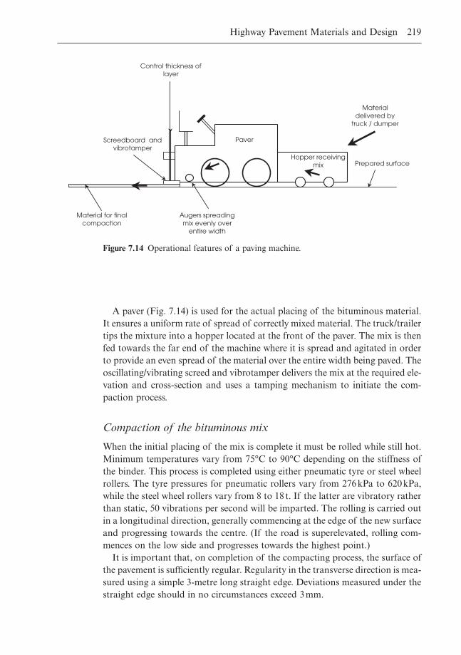
Highway Pavement Materials and Design 219
Hopper receiving mix
Control thickness of layer
Paver
Augers spreading mix evenly over
entire width
Screedboard and vibrotamper
Material for final compaction
Prepared surface
Material delivered by
truck / dumper
Figure 7.14 Operational features of a paving machine.
A paver (Fig. 7.14) is used for the actual placing of the bituminous material.It ensures a uniform rate of spread of correctly mixed material. The truck/trailertips the mixture into a hopper located at the front of the paver. The mix is thenfed towards the far end of the machine where it is spread and agitated in orderto provide an even spread of the material over the entire width being paved. Theoscillating/vibrating screed and vibrotamper delivers the mix at the required ele-vation and cross-section and uses a tamping mechanism to initiate the com-paction process.
Compaction of the bituminous mix
When the initial placing of the mix is complete it must be rolled while still hot.Minimum temperatures vary from 75°C to 90°C depending on the stiffness ofthe binder. This process is completed using either pneumatic tyre or steel wheelrollers. The tyre pressures for pneumatic rollers vary from 276kPa to 620kPa,while the steel wheel rollers vary from 8 to 18 t. If the latter are vibratory ratherthan static, 50 vibrations per second will be imparted. The rolling is carried outin a longitudinal direction, generally commencing at the edge of the new surfaceand progressing towards the centre. (If the road is superelevated, rolling com-mences on the low side and progresses towards the highest point.)
It is important that, on completion of the compacting process, the surface ofthe pavement is sufficiently regular. Regularity in the transverse direction is mea-sured using a simple 3-metre long straight edge. Deviations measured under thestraight edge should in no circumstances exceed 3mm.
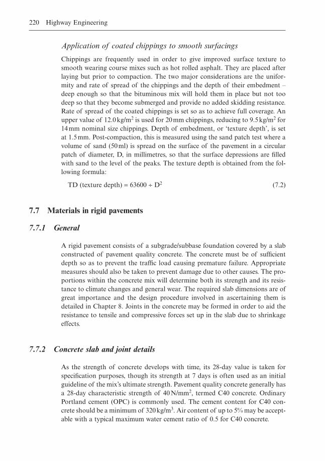
220 Highway Engineering
Application of coated chippings to smooth surfacings
Chippings are frequently used in order to give improved surface texture tosmooth wearing course mixes such as hot rolled asphalt. They are placed afterlaying but prior to compaction. The two major considerations are the unifor-mity and rate of spread of the chippings and the depth of their embedment –deep enough so that the bituminous mix will hold them in place but not toodeep so that they become submerged and provide no added skidding resistance.Rate of spread of the coated chippings is set so as to achieve full coverage. Anupper value of 12.0kg/m2 is used for 20mm chippings, reducing to 9.5kg/m2 for14mm nominal size chippings. Depth of embedment, or ‘texture depth’, is setat 1.5mm. Post-compaction, this is measured using the sand patch test where avolume of sand (50ml) is spread on the surface of the pavement in a circularpatch of diameter, D, in millimetres, so that the surface depressions are filledwith sand to the level of the peaks. The texture depth is obtained from the fol-lowing formula:
TD (texture depth) = 63600 ∏ D2 (7.2)
7.7 Materials in rigid pavements
7.7.1 General
A rigid pavement consists of a subgrade/subbase foundation covered by a slabconstructed of pavement quality concrete. The concrete must be of sufficientdepth so as to prevent the traffic load causing premature failure. Appropriatemeasures should also be taken to prevent damage due to other causes. The pro-portions within the concrete mix will determine both its strength and its resis-tance to climate changes and general wear. The required slab dimensions are ofgreat importance and the design procedure involved in ascertaining them isdetailed in Chapter 8. Joints in the concrete may be formed in order to aid theresistance to tensile and compressive forces set up in the slab due to shrinkageeffects.
7.7.2 Concrete slab and joint details
As the strength of concrete develops with time, its 28-day value is taken for specification purposes, though its strength at 7 days is often used as an initialguideline of the mix’s ultimate strength. Pavement quality concrete generally hasa 28-day characteristic strength of 40N/mm2, termed C40 concrete. OrdinaryPortland cement (OPC) is commonly used. The cement content for C40 con-crete should be a minimum of 320kg/m3. Air content of up to 5% may be accept-able with a typical maximum water cement ratio of 0.5 for C40 concrete.
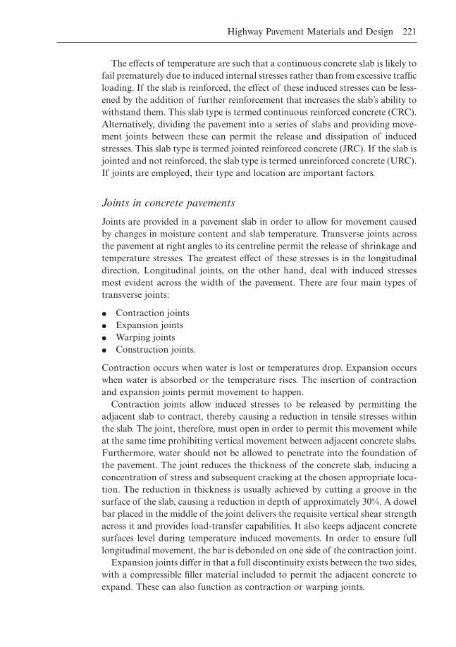
The effects of temperature are such that a continuous concrete slab is likely tofail prematurely due to induced internal stresses rather than from excessive trafficloading. If the slab is reinforced, the effect of these induced stresses can be less-ened by the addition of further reinforcement that increases the slab’s ability towithstand them. This slab type is termed continuous reinforced concrete (CRC).Alternatively, dividing the pavement into a series of slabs and providing move-ment joints between these can permit the release and dissipation of inducedstresses. This slab type is termed jointed reinforced concrete (JRC). If the slab isjointed and not reinforced, the slab type is termed unreinforced concrete (URC).If joints are employed, their type and location are important factors.
Joints in concrete pavements
Joints are provided in a pavement slab in order to allow for movement causedby changes in moisture content and slab temperature. Transverse joints acrossthe pavement at right angles to its centreline permit the release of shrinkage andtemperature stresses. The greatest effect of these stresses is in the longitudinaldirection. Longitudinal joints, on the other hand, deal with induced stressesmost evident across the width of the pavement. There are four main types oftransverse joints:
� Contraction joints� Expansion joints� Warping joints� Construction joints.
Contraction occurs when water is lost or temperatures drop. Expansion occurswhen water is absorbed or the temperature rises. The insertion of contractionand expansion joints permit movement to happen.
Contraction joints allow induced stresses to be released by permitting theadjacent slab to contract, thereby causing a reduction in tensile stresses withinthe slab. The joint, therefore, must open in order to permit this movement whileat the same time prohibiting vertical movement between adjacent concrete slabs.Furthermore, water should not be allowed to penetrate into the foundation ofthe pavement. The joint reduces the thickness of the concrete slab, inducing aconcentration of stress and subsequent cracking at the chosen appropriate loca-tion. The reduction in thickness is usually achieved by cutting a groove in thesurface of the slab, causing a reduction in depth of approximately 30%. A dowelbar placed in the middle of the joint delivers the requisite vertical shear strengthacross it and provides load-transfer capabilities. It also keeps adjacent concretesurfaces level during temperature induced movements. In order to ensure fulllongitudinal movement, the bar is debonded on one side of the contraction joint.
Expansion joints differ in that a full discontinuity exists between the two sides,with a compressible filler material included to permit the adjacent concrete toexpand. These can also function as contraction or warping joints.
Highway Pavement Materials and Design 221
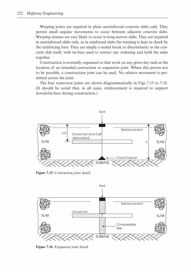
222 Highway Engineering
Warping joints are required in plain unreinforced concrete slabs only. Theypermit small angular movements to occur between adjacent concrete slabs.Warping stresses are very likely to occur in long narrow slabs. They are requiredin unreinforced slabs only, as in reinforced slabs the warping is kept in check bythe reinforcing bars. They are simply a sealed break or discontinuity in the con-crete slab itself, with tie-bars used to restrict any widening and hold the sidestogether.
Construction is normally organised so that work on any given day ends at thelocation of an intended contraction or expansion joint. Where this proves notto be possible, a construction joint can be used. No relative movement is per-mitted across the joint.
The four transverse joints are shown diagrammatically in Figs 7.15 to 7.18.(It should be noted that, in all cases, reinforcement is required to supportdowels/tie-bars during construction.)
SLAB SLAB
Dowel bar (one half debonded)
Reinforcement
Seal
Crack inducer
h/2
h
SUBBASE
Figure 7.15 Contraction joint detail.
SLAB SLAB
Compressible filler
Dowel bar
Reinforcement
Seal
SUBBASE
Figure 7.16 Expansion joint detail.
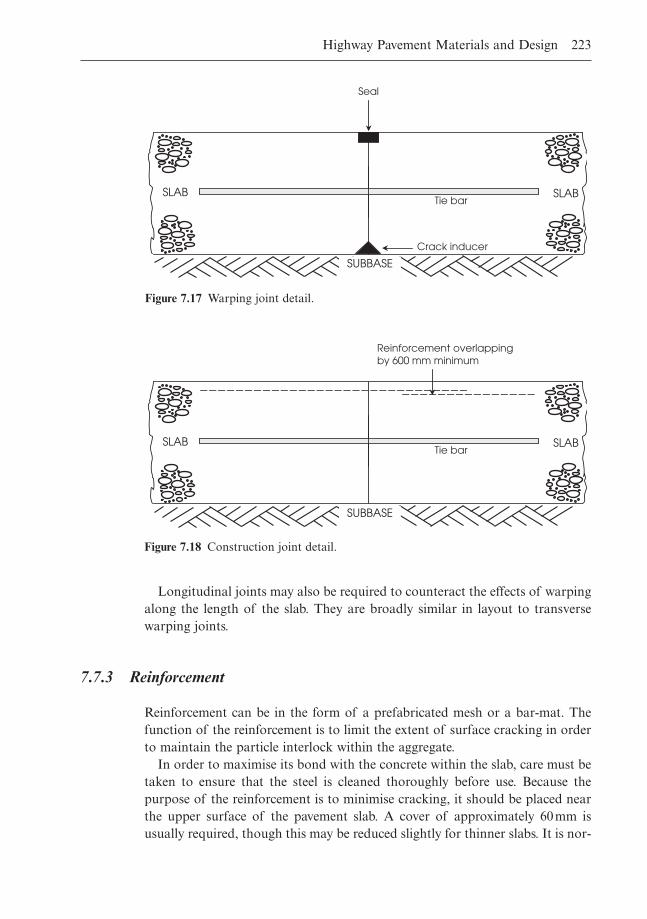
Highway Pavement Materials and Design 223
Longitudinal joints may also be required to counteract the effects of warpingalong the length of the slab. They are broadly similar in layout to transversewarping joints.
7.7.3 Reinforcement
Reinforcement can be in the form of a prefabricated mesh or a bar-mat. Thefunction of the reinforcement is to limit the extent of surface cracking in orderto maintain the particle interlock within the aggregate.
In order to maximise its bond with the concrete within the slab, care must betaken to ensure that the steel is cleaned thoroughly before use. Because thepurpose of the reinforcement is to minimise cracking, it should be placed nearthe upper surface of the pavement slab. A cover of approximately 60mm isusually required, though this may be reduced slightly for thinner slabs. It is nor-
SLAB SLAB
Seal
Crack inducer
SUBBASE
Tie bar
Figure 7.17 Warping joint detail.
SLAB SLAB
Reinforcement overlapping by 600 mm minimum
SUBBASE
Tie bar
Figure 7.18 Construction joint detail.
mally stopped approximately 125mm from the edge of a slab, 100mm from alongitudinal joint and 300mm from any transverse joint.
Transverse lapping of reinforcement within a pavement slab will normally bein the order of 300mm.
7.7.4 Construction of concrete road surfacings
There are a number of key issues that must be addressed in order to properlyconstruct a concrete pavement. These include the positioning of the reinforce-ment in the concrete, the correct forming of both joints and slabs and the chosenmethod of construction, be it mechanised or manual.
Concrete paving is a dynamic and vigorous process, so it is imperative thatthe steel reinforcement is kept firmly in place throughout. In particular, chairsmade from bent reinforcing bars permit the mesh or fabric reinforcement at thetop of the slab to be secured throughout the concreting process. These chairsshould be strong enough to take the weight of workers required to walk overthem during the concreting process. Crack inducers must also be firmly con-nected to the subbase.
Dowel bars used in expansion and contraction joints are usually positionedon metal cradles so that they will not move from their required position whilethe concrete is being placed and compacted. These cradles, however, should notextend across the line of the joint. Tie-bars in warping joints are also normallypart of a rigid construction that allows them to be firmly secured to the sup-porting subbase, while those in construction joints can be inserted into the sideof the pavement slab and recompacted. Alternatively, both dowels and tie-barscan be vibrated into position.
Where the top of the pavement foundation consists of unbound material, itis possible that grout from the concreting process may leak into it. To preventthis occurring, and to minimise frictional forces, a heavy-duty polythene sepa-ration membrane is positioned between the foundation and the jointed concretepavement.
The pavement slab can be constructed in one or two layers. Two layers couldbe employed where an air-entrained upper layer is being installed or for ease inthe placement of reinforcement, where the reinforcement could be placed on thelower layer after it has been compacted, thereby obviating the need for sup-porting chairs.
On large pavement construction projects, continuous concreting is the mosteconomic method of placement. Within it, the paver moves past joint positions,requiring that crack inducers, dowels and tie-bars be kept in position by methodsreferred to above. Purpose-built highway formwork is typically made of steel,held in position by road pins driven through flanges in the form and into thepavement foundation immediately below. Once the steel reinforcement and theformwork are in place, the concreting can commence.
224 Highway Engineering
Mechanised paving allows a higher quality concrete finish to be attained. Thespreading, compacting and finishing of the pavement involves use of a fixed-form or slip-form paving train.
Fixed-form paving uses steel forms or a preconstructed concrete edge-beamto retain the concrete, using machine rails to support and guide the individualitems of plant utilised in the pavement construction process. A train of machines,each individually operated, run along the rails, executing the basic tasks of:
� Spreading the concrete� Compacting it by vibration� Finishing the surface.
Machines for dowel and joint forming that leave the surface of the concrete withthe required texture and the addition of curing compounds may also be includedwithin the process. The machines themselves may be manually propelled, self-powered or towed along the rail.
Typical types of machinery used in a fixed-form paving train are:
(1) Feeder – receives concrete as it arrives at the required location(2) Spreader – distributes the concrete across the full width of the pour in ques-
tion, discharging it at a controlled rate(3) Rotary strike-off paddles and compaction beams – regulate the concrete
by trimming any irregularities in the concrete and vibrate its surface(4) Dowel/tie-bar placers – place these elements in the appropriate joints either
manually or by vibration(5) Joint groove formers and finishers – grooves formed by a knife travelling
within the plastic concrete (wet-formed). Otherwise, a vibrating blade canbe used to form them when the concrete has hardened sufficiently
(6) Final finishing equipment – additional compaction and regulation of theconcrete after the dowel and tie-bars have been put in place. (Machine usestwo oblique finishing beams oscillating in opposite directions to achieve auniform finish to the surface of the concrete)
(7) Curing compound sprayer(8) Protective tentage.
The sequence of operations for two-layer placement with a fixed-form paver isillustrated in Fig. 7.19.
The previous method is analogous to manually placing the concrete. Theprocess can also be completed without using fixed-forms. This process is calledslip-form paving. It works on the basis that the sides of the pavement slab willsupport themselves before an initial set has been developed within the concrete.It produces a fully compacted slab. It cannot therefore be subsequently disturbedin order to place dowel or tie-bars, as the surrounding concrete could not thenbe properly made good. The slip-form paver spreads, compacts and finishes theconcrete with only the forming and finishing of the joint grooves, texturing andcuring done using other pieces of equipment.
Highway Pavement Materials and Design 225
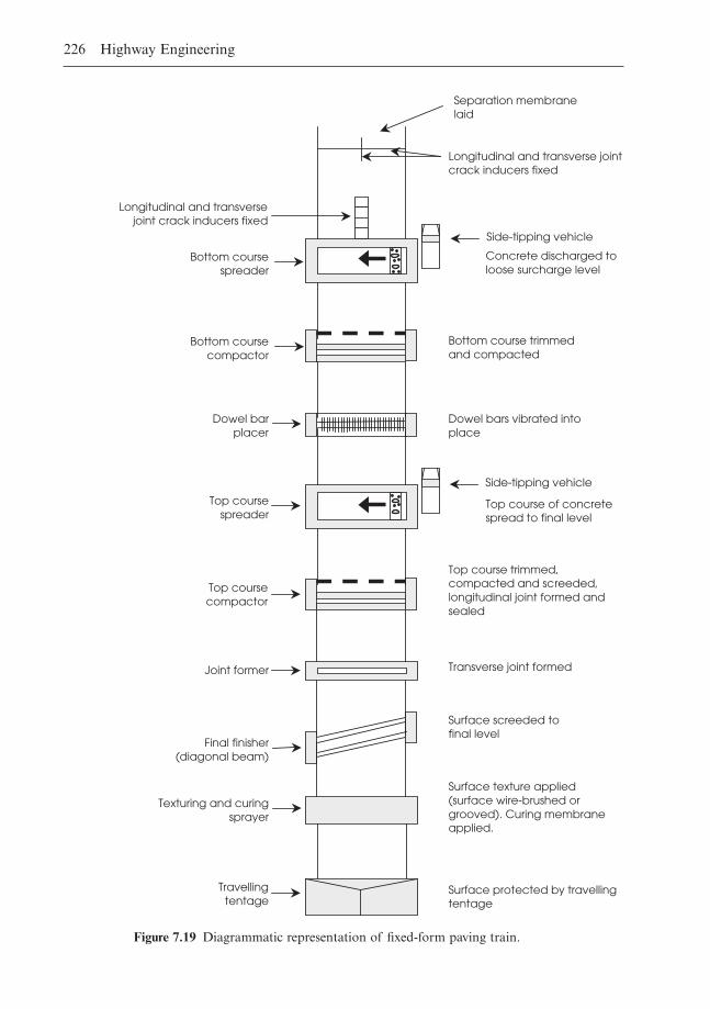
226 Highway Engineering
Concrete discharged to loose surcharge level
Bottom course trimmed and compacted
Top course of concrete spread to final level
Surface protected by travelling tentage
Dowel bars vibrated into place
Longitudinal and transversejoint crack inducers fixed
Side-tipping vehicle
Side-tipping vehicle
Separation membrane laid
Longitudinal and transverse joint crack inducers fixed
Bottom coursespreader
Bottom coursecompactor
Dowel bar placer
Top course spreader
Top course trimmed, compacted and screeded, longitudinal joint formed and sealed
Top course compactor
Transverse joint formed Joint former
Surface screeded to final level
Final finisher (diagonal beam)
Surface texture applied (surface wire-brushed or grooved). Curing membrane applied.
Texturing and curingsprayer
Travelling tentage
Figure 7.19 Diagrammatic representation of fixed-form paving train.
Both methods work on the basis that the full construction process is com-pleted following one pass over the prepared foundation of the pavement. Afterthe usual curing period the slab can then be subjected to normal traffic loadings.
Equally good results are possible with both types of paving machine. The slip-form paver has certain advantages/disadvantages associated with it:
� A higher output is achievable as less machinery is involved� It will tend to be less expensive as labour costs will be lower due to the
increased level of automation.
But:
� Edge slump may occur just after the concrete has left the paver� Greater stockpiles of raw materials such as cement, steel mesh and aggre-
gate are needed in advance of the operation in order to ensure continuedoutput from the paving train
� The contractor operating it may be more vulnerable to weather conditions� A minor quality control failure can cause the entire system to come to a
sudden stop.
7.7.5 Curing and skid resistance
Concrete curing is an essential step in achieving a good quality finished product.It requires that both the temperature and moisture content of the mix be main-tained so that it can continue to gain strength with time. If moisture is lost dueto exposure to sunlight and wind, shrinkage cracks will develop. Such problemsdue to moisture loss can be avoided if the surface of the concrete is kept moistfor at least seven days. This is usually achieved by mechanically spraying the fin-ished surface, with exposure to rain avoided with the use of a travelling tentageas indicated in Fig. 7.19.
Immediately prior to the curing process, the surface should be textured inorder to give it adequate wet-road skidding resistance. It is extremely importantto get the texture to the correct level of quality at the time of construction as potential difficulties may arise with subsequent surface maintenance dur-ing its design life. Good skid resistance requires sufficient microtexture andmacrotexture.
Macrotexture permits most of the rainwater caught between the tyres and thesurface of the highway to drain rapidly and depends on grooves being devel-oped on the surface of the mix in order to ‘texture’ it. Microtexture, on the otherhand, depends on the use of fine aggregate within the mix. It must have abrasion-resistance properties such that the particles of sand stand proud of thematrix of the hardened cement paste while subject to traffic loading, thereforeallowing it to penetrate the remaining film of water and maintain tyre contact
Highway Pavement Materials and Design 227
with the surface. The required macrotexture of the surface is achieved by wire-brushing or grooving.
Wire-brushing is done either manually or mechanically from a skewed travel-ling bridge moving along the line of the pavement. The wire brush is usually aminimum of 450mm long. Grooving is done using a vibrating plate movingacross the width of the finished pavement slab forming random grooves. Theyhave a nominal size of 6mm by 6mm, providing excellent surface water drainageproperties. A high level of wet-road skid resistance is obtained by deep groov-ing, but problems may arise with higher tyre noise.
7.8 References
Black, W.P.M. & Lister, N.W. (1979) The strength of clay fill subgrades: its prediction inrelation to road performance. Department of the Environment, Department of Trans-port. TRRL Report LR 889. Transport and Road Research Laboratory, Crowthorne,UK.
BSI (1984) BS 434 Parts 1 and 2 Bitumen Road Emulsions (Anionic and Cationic). BritishStandards Institution, London.
BSI (1990a) BS 1377 Methods of test for soils for civil engineering purposes. British Stan-dards Institution, London.
BSI (1990b) BS 3690 Part 1 Bitumens for Building and Civil Engineering: Specification forBitumens for Roads and Other Paved Areas. British Standards Institution, London.
BSI (1992) BS 594 Hot rolled asphalt for roads and other paved areas. British StandardsInstitution, London.
DoT (1994) Foundations, HD 25/94. Design Manual for Roads and Bridges, Volume 7:Pavement Design and Maintenance. The Stationery Office, London, UK.
DoT (1996) Traffic Assessment, HD 24/96. Design Manual for Roads and Bridges, Volume7: Pavement Design and Maintenance. The Stationery Office, London, UK.
DoT (1999) General Information, HD 23/99. Design Manual for Roads and Bridges,Volume 7: Pavement Design and Maintenance. The Stationery Office, London, UK.
DoT (2001) Pavement design and construction, HD 26/01. Design Manual for Roads andBridges, Volume 7: Pavement Design and Maintenance. The Stationery Office, London,UK.
O’Flaherty, C.A. (2002) Highways: The location, design, construction and maintenance ofpavements. Butterworth Heinemann, Oxford.
Specification for Highway Works. London: HMSO, 1998.
228 Highway Engineering
Chapter 8
Structural Design of Pavement Thickness
8.1 Introduction
One of the basic requirements for a pavement is that it should be of sufficientthickness to spread the surface loading to a pressure intensity that the underly-ing subgrade is able to withstand, with the pavement itself sufficiently robust todeal with the stresses incident on it. Where required, the pavement should besufficiently thick to prevent damage to a frost-susceptible subgrade. Thicknessis thus a central factor in the pavement design process.
The thickness designs in this chapter are based on LR1132 (Powell et al., 1984)for flexible pavements and RR87 (Mayhew & Harding, 1987) for rigid con-struction. However, these basic designs are modified and updated based on laterresearch as detailed in HD 26/01 (DoT, 2001). The pavement thickness designmethodologies for the two different categories of pavement type are treated separately below.
In order to reflect European harmonisation, the names of the various pave-ment layers have been altered within the context of thickness design, as seen inFig. 8.1.
8.2 Flexible pavements
8.2.1 General
The pavement should be neither too thick nor too thin. If it is too thick, thecost will become excessive. If it is too thin, it will fail to protect the underlyingunbound layers, causing rutting at formation level.
A flexible pavement is defined as one where the surface course, binder courseand base materials are bitumen bound. Permitted materials include hot rolledasphalt (HRA), high density macadam (HDM), dense bitumen macadam(DBM) and dense bitumen macadam with 50-penetration bitumen (DBM50).Flexible composite pavements involve surface course and upper base materialsbound with macadam built on a lower base of cement bound material (CBM).Wearing courses are either 45mm or 50mm of hot rolled asphalt or 50mm of
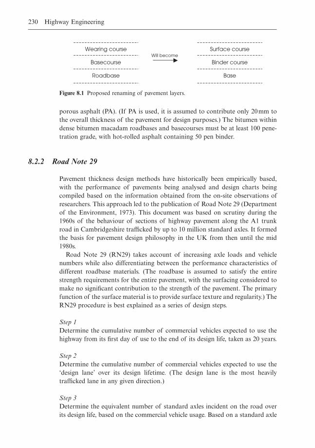
porous asphalt (PA). (If PA is used, it is assumed to contribute only 20mm tothe overall thickness of the pavement for design purposes.) The bitumen withindense bitumen macadam roadbases and basecourses must be at least 100 pene-tration grade, with hot-rolled asphalt containing 50 pen binder.
8.2.2 Road Note 29
Pavement thickness design methods have historically been empirically based,with the performance of pavements being analysed and design charts being compiled based on the information obtained from the on-site observations ofresearchers. This approach led to the publication of Road Note 29 (Departmentof the Environment, 1973). This document was based on scrutiny during the1960s of the behaviour of sections of highway pavement along the A1 trunkroad in Cambridgeshire trafficked by up to 10 million standard axles. It formedthe basis for pavement design philosophy in the UK from then until the mid1980s.
Road Note 29 (RN29) takes account of increasing axle loads and vehiclenumbers while also differentiating between the performance characteristics ofdifferent roadbase materials. (The roadbase is assumed to satisfy the entirestrength requirements for the entire pavement, with the surfacing considered tomake no significant contribution to the strength of the pavement. The primaryfunction of the surface material is to provide surface texture and regularity.) TheRN29 procedure is best explained as a series of design steps.
Step 1Determine the cumulative number of commercial vehicles expected to use thehighway from its first day of use to the end of its design life, taken as 20 years.
Step 2Determine the cumulative number of commercial vehicles expected to use the‘design lane’ over its design lifetime. (The design lane is the most heavily trafficked lane in any given direction.)
Step 3Determine the equivalent number of standard axles incident on the road overits design life, based on the commercial vehicle usage. Based on a standard axle
230 Highway Engineering
Wearing course
Basecourse
Roadbase
Surface course
Binder course
Base
Will become
Figure 8.1 Proposed renaming of pavement layers.
of 80kN, the required value is obtained from the product of the cumulativenumber of commercial vehicles and a term called the damage factor which variesfor different road types. The maximum value of this conversion factor is 1.08,used for motorways and trunk roads designed to cater for over 1000 commer-cial vehicles per day in each direction.
For a motorway:
Equivalent No. of standard axles = No. of commercial vehicles ¥ 1.08 (8.1)
Step 4Determine the subbase thickness. This is dependent on both the CBR of thesubgrade and the cumulative number of standard axles over the design life ofthe highway. For a cumulative number of standard axles of 1 million (1msa), aminimum subbase thickness of 150mm is required where the CBR is greaterthan 6%, rising to 440mm where the CBR is 2%. Where the CBR is less than2%, an additional 150mm of subbase should be added to that required for aCBR of 2%. The CBR of the subbase should be at least 30%. If the CBR ofthe subgrade is in excess of this value, no subbase need be used.
Step 5Determine the roadbase and surfacing thickness. This parameter depends purelyon the cumulative number of standard axles over the pavement’s design life. Forcumulative standard axles in excess of 10 million, the surfacing should be 100mm thick (60mm basecourse plus 40mm wearing course). If dense bitumenmacadam is used, a roadbase thickness of just under 150mm is required to caterfor 10msa, giving a total bound thickness of 250mm.
8.2.3 LR1132
Road Note 29 was the sole officially recognised pavement design methodologythroughout the 1970s and early 1980s. While it was considered to be generallyeffective, it had certain inherent deficiencies:
� It was seen as unresponsive both to improvements in the quality of availableraw materials and to changes in construction processes.
� The RN29 method is valid for designs up to 40msa. Many highways were,by the mid 1980s, well in excess of 50msa, with some approaching 150msaover their 20-year design life.
� The 20-year design life implied that, after this period, a surface rut of 20mmor more, or severe cracking or crazing had developed. The pavement wasthen considered to be in a failed state and in need of major strengtheningor partial reconstruction. It has been shown that attempting to strengthen a pavement damaged to such an extent did not automatically result in satisfactory performance afterwards.
Structural Design of Pavement Thickness 231
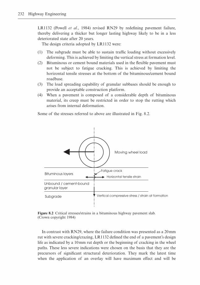
LR1132 (Powell et al., 1984) revised RN29 by redefining pavement failure,thereby delivering a thicker but longer lasting highway likely to be in a less deteriorated state after 20 years.
The design criteria adopted by LR1132 were:
(1) The subgrade must be able to sustain traffic loading without excessivelydeforming. This is achieved by limiting the vertical stress at formation level.
(2) Bituminous or cement bound materials used in the flexible pavement mustnot be subject to fatigue cracking. This is achieved by limiting the horizontal tensile stresses at the bottom of the bituminous/cement boundroadbase.
(3) The load spreading capability of granular subbases should be enough toprovide an acceptable construction platform.
(4) When a pavement is composed of a considerable depth of bituminousmaterial, its creep must be restricted in order to stop the rutting whicharises from internal deformation.
Some of the stresses referred to above are illustrated in Fig. 8.2.
232 Highway Engineering
Moving wheel load
Bituminous layers
Unbound / cement-bound granular layer
Horizontal tensile strain
Fatigue crack
Vertical compressive stress / strain at formation Subgrade
Figure 8.2 Critical stresses/strains in a bituminous highway pavement slab.(Crown copyright 1984)
In contrast with RN29, where the failure condition was presented as a 20mmrut with severe cracking/crazing, LR1132 defined the end of a pavement’s designlife as indicated by a 10mm rut depth or the beginning of cracking in the wheelpaths. These less severe indications were chosen on the basis that they are theprecursors of significant structural deterioration. They mark the latest timewhen the application of an overlay will have maximum effect and will be
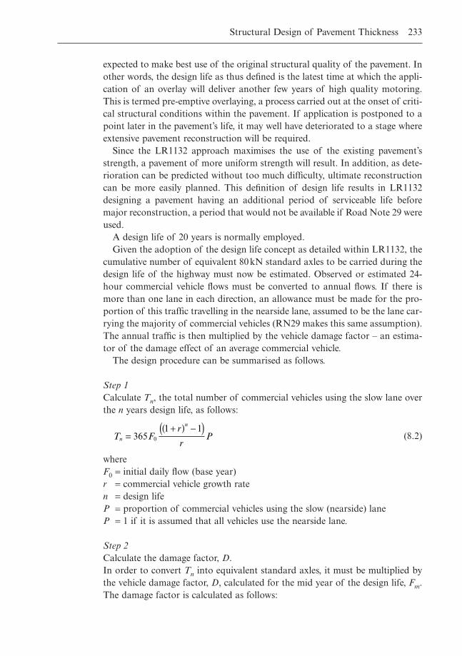
expected to make best use of the original structural quality of the pavement. Inother words, the design life as thus defined is the latest time at which the appli-cation of an overlay will deliver another few years of high quality motoring.This is termed pre-emptive overlaying, a process carried out at the onset of criti-cal structural conditions within the pavement. If application is postponed to apoint later in the pavement’s life, it may well have deteriorated to a stage whereextensive pavement reconstruction will be required.
Since the LR1132 approach maximises the use of the existing pavement’sstrength, a pavement of more uniform strength will result. In addition, as dete-rioration can be predicted without too much difficulty, ultimate reconstructioncan be more easily planned. This definition of design life results in LR1132designing a pavement having an additional period of serviceable life beforemajor reconstruction, a period that would not be available if Road Note 29 wereused.
A design life of 20 years is normally employed.Given the adoption of the design life concept as detailed within LR1132, the
cumulative number of equivalent 80kN standard axles to be carried during thedesign life of the highway must now be estimated. Observed or estimated 24-hour commercial vehicle flows must be converted to annual flows. If there ismore than one lane in each direction, an allowance must be made for the pro-portion of this traffic travelling in the nearside lane, assumed to be the lane car-rying the majority of commercial vehicles (RN29 makes this same assumption).The annual traffic is then multiplied by the vehicle damage factor – an estima-tor of the damage effect of an average commercial vehicle.
The design procedure can be summarised as follows.
Step 1Calculate Tn, the total number of commercial vehicles using the slow lane overthe n years design life, as follows:
(8.2)
whereF0 = initial daily flow (base year)r = commercial vehicle growth raten = design lifeP = proportion of commercial vehicles using the slow (nearside) laneP = 1 if it is assumed that all vehicles use the nearside lane.
Step 2Calculate the damage factor, D.In order to convert Tn into equivalent standard axles, it must be multiplied bythe vehicle damage factor, D, calculated for the mid year of the design life, Fm.The damage factor is calculated as follows:
T Fr
rPn
n
=+( ) -( )
3651 1
0
Structural Design of Pavement Thickness 233
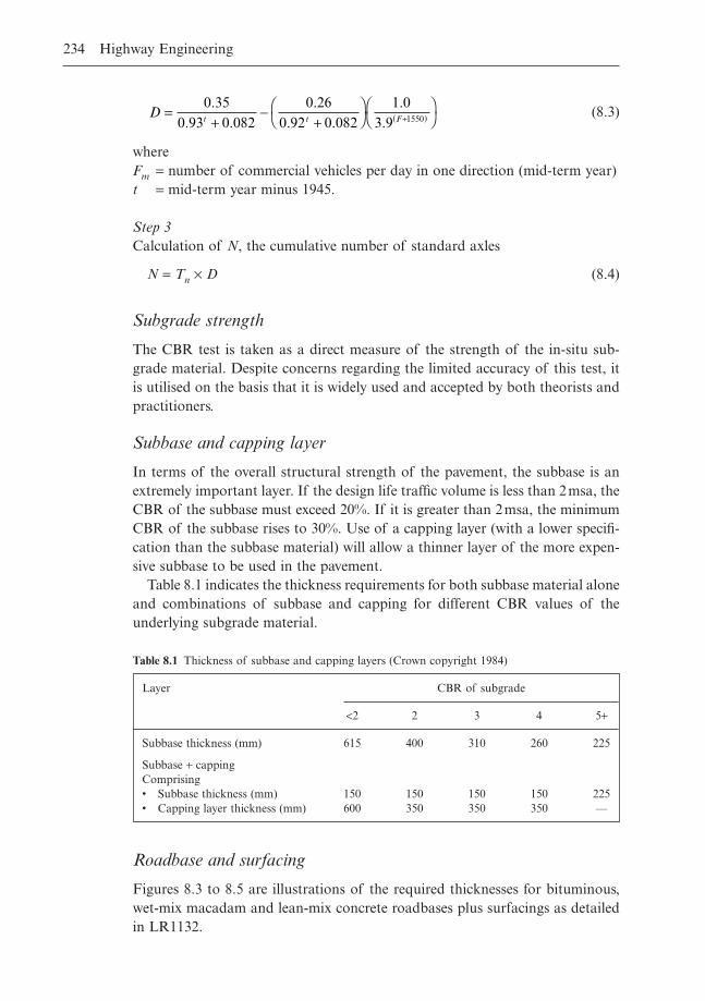
(8.3)
whereFm = number of commercial vehicles per day in one direction (mid-term year)t = mid-term year minus 1945.
Step 3Calculation of N, the cumulative number of standard axles
N = Tn ¥ D (8.4)
Subgrade strength
The CBR test is taken as a direct measure of the strength of the in-situ sub-grade material. Despite concerns regarding the limited accuracy of this test, itis utilised on the basis that it is widely used and accepted by both theorists andpractitioners.
Subbase and capping layer
In terms of the overall structural strength of the pavement, the subbase is anextremely important layer. If the design life traffic volume is less than 2msa, theCBR of the subbase must exceed 20%. If it is greater than 2msa, the minimumCBR of the subbase rises to 30%. Use of a capping layer (with a lower specifi-cation than the subbase material) will allow a thinner layer of the more expen-sive subbase to be used in the pavement.
Table 8.1 indicates the thickness requirements for both subbase material aloneand combinations of subbase and capping for different CBR values of theunderlying subgrade material.
D t t F=
+-
+ÊË
ˆ¯ÊË
ˆ¯∏( )
0 350 93 0 082
0 260 92 0 082
1 03 9 1550
.. .
.. .
..
234 Highway Engineering
Layer CBR of subgrade
<2 2 3 4 5+
Subbase thickness (mm) 615 400 310 260 225
Subbase + cappingComprising• Subbase thickness (mm) 150 150 150 150 225• Capping layer thickness (mm) 600 350 350 350 —
Table 8.1 Thickness of subbase and capping layers (Crown copyright 1984)
Roadbase and surfacing
Figures 8.3 to 8.5 are illustrations of the required thicknesses for bituminous,wet-mix macadam and lean-mix concrete roadbases plus surfacings as detailedin LR1132.
Structural Design of Pavement Thickness 235
Cumulative traffic (msa)
Thickness of bound layers (mm)
0.01 1.0 100
100
200
400
300
Subgrade CBR = 5% Subbase thickness = 225 mm Probability of survival = 85%
Roadbase + Surfacing
Figure 8.3 Design curve for highways with bituminous roadbase. (Crown copyright 1984)
Cumulative traffic (msa)
Thickness of bound layers (mm)
0.01 1.0 100
100
200
400
300
Subgrade CBR = 5% Subbase thickness = 225 mm Probability of survival = 85%
Roadbase
Surfacing
Figure 8.4 Design curve for highways with wet-mix roadbase. (Crown copyright 1984)
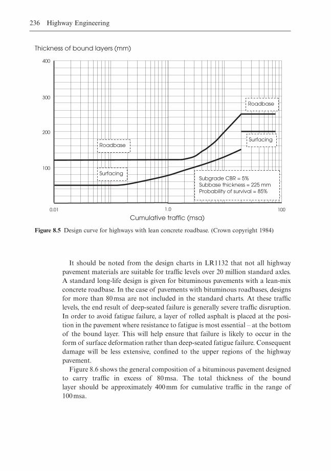
It should be noted from the design charts in LR1132 that not all highwaypavement materials are suitable for traffic levels over 20 million standard axles.A standard long-life design is given for bituminous pavements with a lean-mixconcrete roadbase. In the case of pavements with bituminous roadbases, designsfor more than 80msa are not included in the standard charts. At these trafficlevels, the end result of deep-seated failure is generally severe traffic disruption.In order to avoid fatigue failure, a layer of rolled asphalt is placed at the posi-tion in the pavement where resistance to fatigue is most essential – at the bottomof the bound layer. This will help ensure that failure is likely to occur in theform of surface deformation rather than deep-seated fatigue failure. Consequentdamage will be less extensive, confined to the upper regions of the highway pavement.
Figure 8.6 shows the general composition of a bituminous pavement designedto carry traffic in excess of 80msa. The total thickness of the bound layer should be approximately 400mm for cumulative traffic in the range of100msa.
236 Highway Engineering
Cumulative traffic (msa)
Thickness of bound layers (mm)
0.01 1.0 100
100
200
400
300
Subgrade CBR = 5% Subbase thickness = 225 mm Probability of survival = 85%
Roadbase
Surfacing
Surfacing
Roadbase
Figure 8.5 Design curve for highways with lean concrete roadbase. (Crown copyright 1984)
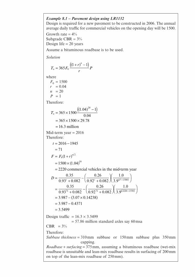
Example 8.1 – Pavement design using LR1132Design is required for a new pavement to be constructed in 2006. The annualaverage daily traffic for commercial vehicles on the opening day will be 1500.
Growth rate = 4%Subgrade CBR = 3%Design life = 20 years
Assume a bituminous roadbase is to be used.
Solution
whereF0 = 1500r = 0.04n = 20P = 1
Therefore:
Mid-term year = 2016Therefore:
Design traffic = 16.3 ¥ 3.5499= 57.86 million standard axles say 60msa
CBR = 3%
Therefore:Subbase thickness = 310mm subbase or 150mm subbase plus 350mm
capping.Roadbase + surfacing = 375mm, assuming a bituminous roadbase (wet-mixroadbase is unsuitable and lean-mix roadbase results in surfacing of 200mmon top of the lean-mix roadbase of 250mm).
t
F F r
D
n
t t F
= -=
= +( )
= ¥ ( )=
=+
-+
ÊË
ˆ¯ÊË
ˆ¯
=+
-+
ÊË
ˆ¯
∏( )
∏
2016 1945
71
1
1500 1 04
2220
0 350 93 0 082
0 260 92 0 082
1 03 9
0 350 93 0 082
0 260 92 0 082
1 03 9
02
10
1500
71 71 2220 1550
.
.. .
.. .
..
.. .
.. .
..
commercial vehicles in the mid-term year
(( )ÊË
ˆ¯
= - ¥( )= -=
3 987 3 07 0 14238
3 987 0 4371
3 5499
. . .
. .
.
Tn = ¥( ) -( )
= ¥ ¥=
365 15001 04 1
0 04365 1500 29 78
16 3
20.
..
. million
T Fr
rPn
n
=+( ) -( )
3651 1
0
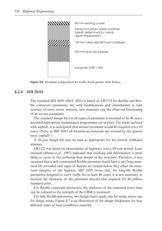
8.2.4 HD 26/01
The standard HD 26/01 (DoT, 2001) is based on LR1132 for flexible and flexi-ble composite pavements, but with modifications and amendments to takeaccount of more recent research, new materials and the observed functioningof in-service pavements.
The standard design life for all types of pavement is assumed to be 40 years,provided appropriate maintenance programmes are in place. For roads surfacedwith asphalt, it is anticipated that surface treatment would be required every 10years. (Note: in HD 26/01 all bituminous materials are covered by the genericterm ‘asphalt’.)
A 20-year design life may be seen as appropriate for less heavily traffickedschemes.
LR1132 was based on observations of highways over a 20-year period. Laterresearch (Munn et al., 1997) indicated that cracking and deformation is morelikely to occur in the surfacing than deeper in the structure. Therefore, it wassurmised that a well-constructed flexible pavement would have a very long struc-tural life provided such signs of distress are treated before they affect the struc-tural integrity of the highway. HD 26/01 notes that, for long-life flexiblepavements designed to carry traffic for at least 40 years, it is not necessary toincrease the thickness of the pavement beyond that required for 80 million standard axles.
For flexible composite pavements, the thickness of the cemented lower basecan be reduced as the strength of the CBM is increased.
For fully flexible pavements, two design charts apply, one for recipe mixes, onefor design mixes. Figure 8.7 is an illustration of the design thicknesses for fourdifferent types of base (roadbase) material:
238 Highway Engineering
40 mm wearing course
Dense macadam upper roadbase (depth determined by overall depth requirement)
125 mm rolled asphalt lower roadbase
225 mm granular subbase
Subgrade (CBR = 5%)
Figure 8.6 Pavement composition for traffic levels greater than 80 msa.
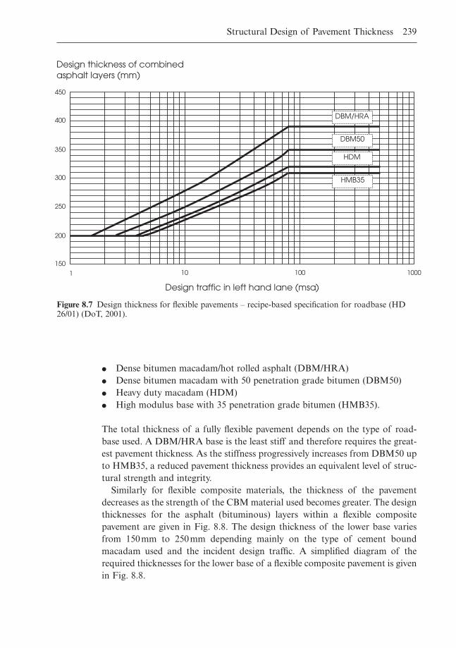
� Dense bitumen macadam/hot rolled asphalt (DBM/HRA)� Dense bitumen macadam with 50 penetration grade bitumen (DBM50)� Heavy duty macadam (HDM)� High modulus base with 35 penetration grade bitumen (HMB35).
The total thickness of a fully flexible pavement depends on the type of road-base used. A DBM/HRA base is the least stiff and therefore requires the great-est pavement thickness. As the stiffness progressively increases from DBM50 upto HMB35, a reduced pavement thickness provides an equivalent level of struc-tural strength and integrity.
Similarly for flexible composite materials, the thickness of the pavementdecreases as the strength of the CBM material used becomes greater. The designthicknesses for the asphalt (bituminous) layers within a flexible composite pavement are given in Fig. 8.8. The design thickness of the lower base variesfrom 150mm to 250mm depending mainly on the type of cement boundmacadam used and the incident design traffic. A simplified diagram of therequired thicknesses for the lower base of a flexible composite pavement is givenin Fig. 8.8.
Structural Design of Pavement Thickness 239
Design traffic in left hand lane (msa)
100010010 1
150
200
250
300
350
400
450
Design thickness of combined asphalt layers (mm)
DBM50
DBM/HRA
HDM
HMB35
Figure 8.7 Design thickness for flexible pavements – recipe-based specification for roadbase (HD26/01) (DoT, 2001).
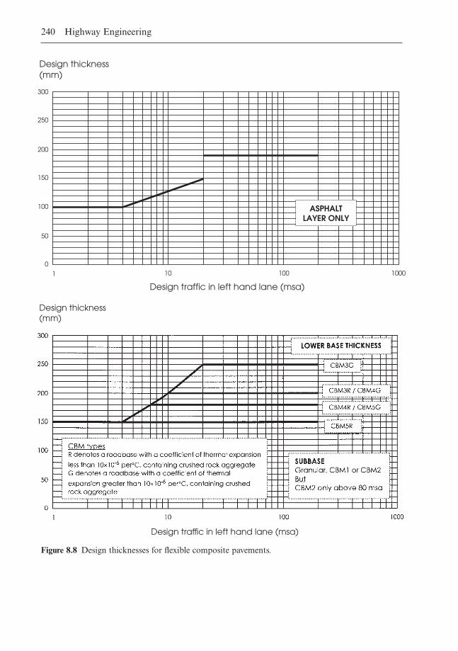
240 Highway Engineering
Design traffic in left hand lane (msa)
1000 100 10 1
0
50
100
150
200
250
300
Design thickness(mm)
ASPHALT LAYER ONLY
Figure 8.8 Design thicknesses for flexible composite pavements.
Design thickness(mm)
Design traffic in left hand lane (msa)

Structural Design of Pavement Thickness 241
Example 8.2A highway is envisaged to carry a traffic loading of 40msa over its designlife. Interpret the necessary asphalt thickness for a wholly bituminous pave-ment using the relevant chart from HD 26/01 (DoT, 2001).
Solution
From Fig. 8.7, the following required thicknesses can be deduced:
(1) For DBM/HRA base: 350mm(2) For DBM50 base: 310mm(3) For HDM base: 290mm(4) For HMB35 base: 280mm.
Note: all thicknesses are rounded up to the nearest 10mm in accordance withthe guidance from HD 26/01.
Example 8.3A highway is envisaged to carry a traffic loading of 30msa over its designlife. Interpret the necessary surfacing and lower base thicknesses for a flexi-ble composite pavement using the relevant chart from HD 26/01.
Solution
From Fig. 8.8, the following information can be deduced.The total asphalt layer required is 190mm. Typically, this would be com-
posed of:
� 40mm HRA wearing course (surface course), overlaying� 50mm basecourse (binder course), overlaying� 100mm roadbase (base).
For DBM/HRA base, required thickness is 350mmThe lower base layer required on a granular subbase is:
� 250mm of CBM3G base, or� 200mm of CBM3R or CBM4G, or� 180mm of CBM4R or CBM5G, or� 150mm of CBM5R.
Note: CBM 5, 4 and 3 are the highest quality cement bound materials,usually prepared at a central plant from batched amounts of processedcrushed gravel or rock.
A very similar result is obtained from LR1132. If one examines Fig. 8.5detailing required thicknesses for a concrete roadbase plus asphalt surfacing:
For a cumulative traffic figure of 30msa:
� Asphalt surfacing thickness = 200mm� Lean-mix concrete roadbase = 250mm.
which is within 10mm of the overall thickness recommended by HD 26/01.
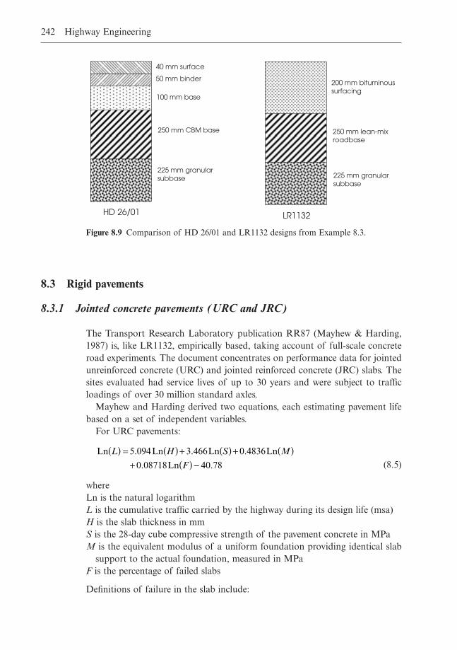
8.3 Rigid pavements
8.3.1 Jointed concrete pavements (URC and JRC)
The Transport Research Laboratory publication RR87 (Mayhew & Harding,1987) is, like LR1132, empirically based, taking account of full-scale concreteroad experiments. The document concentrates on performance data for jointedunreinforced concrete (URC) and jointed reinforced concrete (JRC) slabs. Thesites evaluated had service lives of up to 30 years and were subject to trafficloadings of over 30 million standard axles.
Mayhew and Harding derived two equations, each estimating pavement lifebased on a set of independent variables.
For URC pavements:
(8.5)
whereLn is the natural logarithmL is the cumulative traffic carried by the highway during its design life (msa)H is the slab thickness in mmS is the 28-day cube compressive strength of the pavement concrete in MPaM is the equivalent modulus of a uniform foundation providing identical slab
support to the actual foundation, measured in MPaF is the percentage of failed slabs
Definitions of failure in the slab include:
Ln Ln Ln Ln
Ln
L H S M
F
( ) = ( ) + ( ) + ( )+ ( ) -5 094 3 466 0 4836
0 08718 40 78
. . .
. .
242 Highway Engineering
225 mm granular subbase
40 mm surface
250 mm CBM base
50 mm binder
100 mm base
250 mm lean-mix roadbase
200 mm bituminous surfacing
225 mm granular subbase
HD 26/01 LR1132
Figure 8.9 Comparison of HD 26/01 and LR1132 designs from Example 8.3.
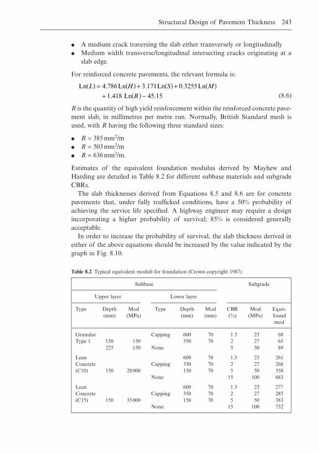
� A medium crack traversing the slab either transversely or longitudinally� Medium width transverse/longitudinal intersecting cracks originating at a
slab edge.
For reinforced concrete pavements, the relevant formula is:
(8.6)
R is the quantity of high yield reinforcement within the reinforced concrete pave-ment slab, in millimetres per metre run. Normally, British Standard mesh isused, with R having the following three standard sizes:
� R = 385mm2/m� R = 503mm2/m� R = 636mm2/m.
Estimates of the equivalent foundation modulus derived by Mayhew andHarding are detailed in Table 8.2 for different subbase materials and subgradeCBRs.
The slab thicknesses derived from Equations 8.5 and 8.6 are for concrete pavements that, under fully trafficked conditions, have a 50% probability ofachieving the service life specified. A highway engineer may require a designincorporating a higher probability of survival; 85% is considered generallyacceptable.
In order to increase the probability of survival, the slab thickness derived ineither of the above equations should be increased by the value indicated by thegraph in Fig. 8.10.
Ln Ln Ln Ln
Ln
L H S M
R
( ) = ( ) + ( ) + ( )+ ( ) -4 786 3 171 0 3255
1 418 45 15
. . .
. .
Structural Design of Pavement Thickness 243
Subbase Subgrade
Upper layer Lower layer
Type Depth Mod Type Depth Mod CBR Mod Equiv.(mm) (MPa) (mm) (mm) (%) (MPa) found
mod
Granular Capping 600 70 1.5 23 68Type 1 150 150 350 70 2 27 65
225 150 None 5 50 89
Lean 600 70 1.5 23 261Concrete Capping 350 70 2 27 268(C10) 150 28000 150 70 5 50 358
None 15 100 683
Lean 600 70 1.5 23 277Concrete Capping 350 70 2 27 285(C15) 150 35000 150 70 5 50 383
None 15 100 732
Table 8.2 Typical equivalent moduli for foundation (Crown copyright 1987)
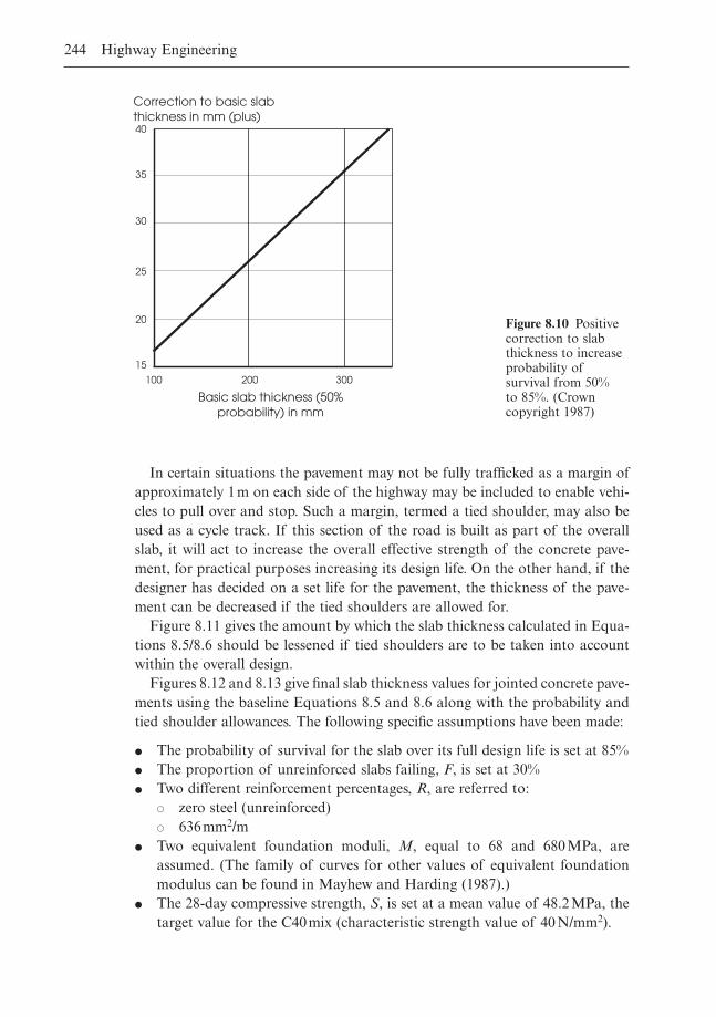
244 Highway Engineering
In certain situations the pavement may not be fully trafficked as a margin ofapproximately 1m on each side of the highway may be included to enable vehi-cles to pull over and stop. Such a margin, termed a tied shoulder, may also beused as a cycle track. If this section of the road is built as part of the overallslab, it will act to increase the overall effective strength of the concrete pave-ment, for practical purposes increasing its design life. On the other hand, if thedesigner has decided on a set life for the pavement, the thickness of the pave-ment can be decreased if the tied shoulders are allowed for.
Figure 8.11 gives the amount by which the slab thickness calculated in Equa-tions 8.5/8.6 should be lessened if tied shoulders are to be taken into accountwithin the overall design.
Figures 8.12 and 8.13 give final slab thickness values for jointed concrete pave-ments using the baseline Equations 8.5 and 8.6 along with the probability andtied shoulder allowances. The following specific assumptions have been made:
� The probability of survival for the slab over its full design life is set at 85%� The proportion of unreinforced slabs failing, F, is set at 30%� Two different reinforcement percentages, R, are referred to:
� zero steel (unreinforced)� 636mm2/m
� Two equivalent foundation moduli, M, equal to 68 and 680MPa, areassumed. (The family of curves for other values of equivalent foundationmodulus can be found in Mayhew and Harding (1987).)
� The 28-day compressive strength, S, is set at a mean value of 48.2MPa, thetarget value for the C40mix (characteristic strength value of 40N/mm2).
40
35
30
25
20
15
100 200 300
Basic slab thickness (50% probability) in mm
Correction to basic slab thickness in mm (plus)
Figure 8.10 Positivecorrection to slabthickness to increaseprobability ofsurvival from 50% to 85%. (Crowncopyright 1987)
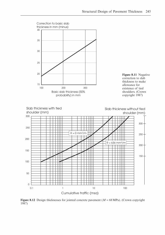
Structural Design of Pavement Thickness 245
40
35
30
25
20
15
100 200 300
Basic slab thickness (50% probability) in mm
Correction to basic slab thickness in mm (minus)
Figure 8.11 Negativecorrection to slabthickness to makeallowance forexistence of tiedshoulders. (Crowncopyright 1987)
Cumulative traffic (msa)
0.1 100 10 1
Slab thickness without tiedshoulder (mm)
50
150
0
100
200
250
300
Slab thickness with tied shoulder (mm)
300
250
200
150
R = 0 mm2/m
R = 636 mm2/m
Figure 8.12 Design thicknesses for jointed concrete pavement (M = 68 MPa). (Crown copyright1987)
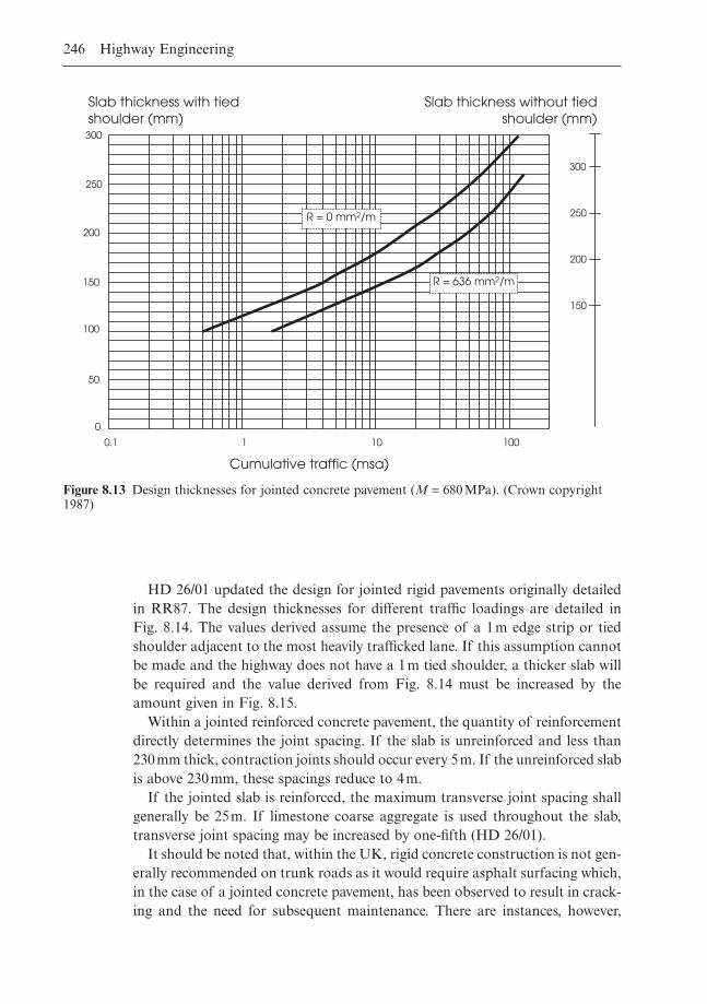
HD 26/01 updated the design for jointed rigid pavements originally detailedin RR87. The design thicknesses for different traffic loadings are detailed in Fig. 8.14. The values derived assume the presence of a 1m edge strip or tiedshoulder adjacent to the most heavily trafficked lane. If this assumption cannotbe made and the highway does not have a 1m tied shoulder, a thicker slab willbe required and the value derived from Fig. 8.14 must be increased by theamount given in Fig. 8.15.
Within a jointed reinforced concrete pavement, the quantity of reinforcementdirectly determines the joint spacing. If the slab is unreinforced and less than230mm thick, contraction joints should occur every 5m. If the unreinforced slabis above 230mm, these spacings reduce to 4m.
If the jointed slab is reinforced, the maximum transverse joint spacing shallgenerally be 25m. If limestone coarse aggregate is used throughout the slab,transverse joint spacing may be increased by one-fifth (HD 26/01).
It should be noted that, within the UK, rigid concrete construction is not gen-erally recommended on trunk roads as it would require asphalt surfacing which,in the case of a jointed concrete pavement, has been observed to result in crack-ing and the need for subsequent maintenance. There are instances, however,
246 Highway Engineering
Slab thickness without tied shoulder (mm)
Cumulative traffic (msa)
0.1 100 10 1
50
150
0
100
200
250
300
Slab thickness with tied shoulder (mm)
300
250
200
150
R = 0 mm2/m
R = 636 mm2/m
Figure 8.13 Design thicknesses for jointed concrete pavement (M = 680 MPa). (Crown copyright1987)
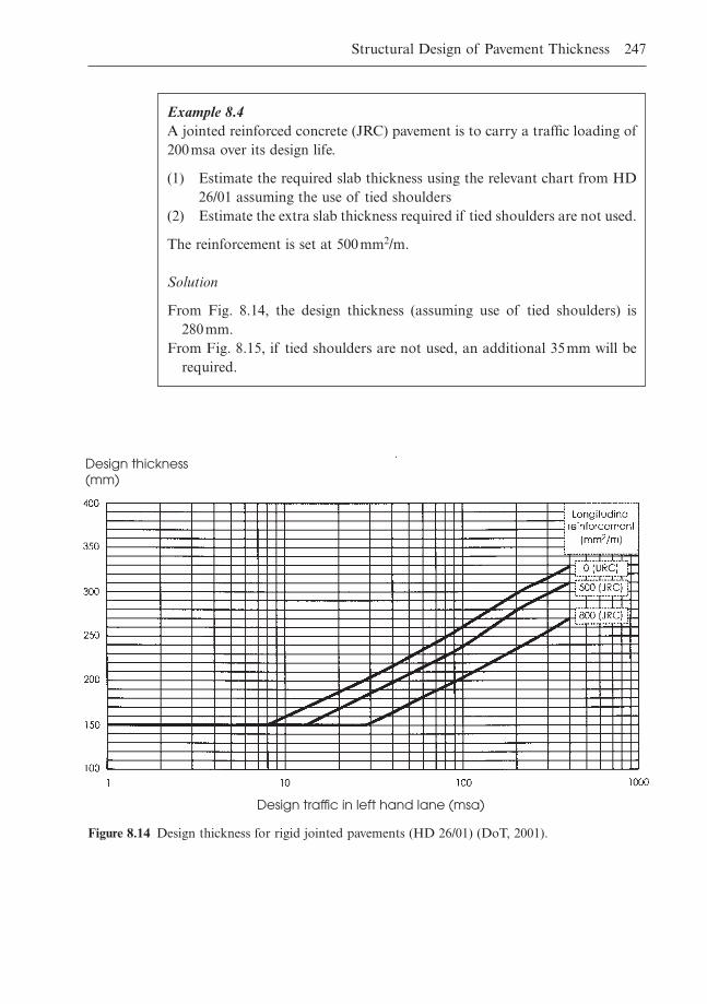
Structural Design of Pavement Thickness 247
Design thickness(mm)
Design traffic in left hand lane (msa)
Figure 8.14 Design thickness for rigid jointed pavements (HD 26/01) (DoT, 2001).
Example 8.4A jointed reinforced concrete (JRC) pavement is to carry a traffic loading of200msa over its design life.
(1) Estimate the required slab thickness using the relevant chart from HD26/01 assuming the use of tied shoulders
(2) Estimate the extra slab thickness required if tied shoulders are not used.
The reinforcement is set at 500mm2/m.
Solution
From Fig. 8.14, the design thickness (assuming use of tied shoulders) is 280mm.
From Fig. 8.15, if tied shoulders are not used, an additional 35mm will be required.
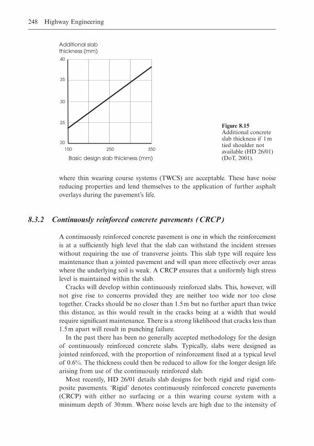
where thin wearing course systems (TWCS) are acceptable. These have noisereducing properties and lend themselves to the application of further asphaltoverlays during the pavement’s life.
8.3.2 Continuously reinforced concrete pavements (CRCP)
A continuously reinforced concrete pavement is one in which the reinforcementis at a sufficiently high level that the slab can withstand the incident stresseswithout requiring the use of transverse joints. This slab type will require lessmaintenance than a jointed pavement and will span more effectively over areaswhere the underlying soil is weak. A CRCP ensures that a uniformly high stresslevel is maintained within the slab.
Cracks will develop within continuously reinforced slabs. This, however, willnot give rise to concerns provided they are neither too wide nor too closetogether. Cracks should be no closer than 1.5m but no further apart than twicethis distance, as this would result in the cracks being at a width that wouldrequire significant maintenance. There is a strong likelihood that cracks less than1.5m apart will result in punching failure.
In the past there has been no generally accepted methodology for the designof continuously reinforced concrete slabs. Typically, slabs were designed asjointed reinforced, with the proportion of reinforcement fixed at a typical levelof 0.6%. The thickness could then be reduced to allow for the longer design lifearising from use of the continuously reinforced slab.
Most recently, HD 26/01 details slab designs for both rigid and rigid com-posite pavements. ‘Rigid’ denotes continuously reinforced concrete pavements(CRCP) with either no surfacing or a thin wearing course system with aminimum depth of 30mm. Where noise levels are high due to the intensity of
248 Highway Engineering
Basic design slab thickness (mm)
40
35
30
25
20
150 250 350
Additional slab thickness (mm)
Figure 8.15Additional concreteslab thickness if 1 mtied shoulder notavailable (HD 26/01)(DoT, 2001).
Structural Design of Pavement Thickness 249
Example 8.5A continuously reinforced concrete pavement is to carry a traffic loading of200msa over its design life.
Estimate the required slab using:
(1) CRCP(2) CRCR.
Give some surfacing options.
Solution
(1) Required reinforced concrete pavement thickness of 230mm with 30mm of thin wearing course system (TWCS)
(2) Required reinforced concrete base thickness of 210mm with the 100mmof surfacing comprising either 45mm hot rolled asphalt (HRA) surface course overlaying 55mm of dense bitumen macadam (DBM)binder course or 15mm of TWCS overlaying 85mm of DBM bindercourse.
traffic on the highway, surfacing materials can significantly lower noise emis-sions generated by vehicles. Thin wearing course systems can be significantlyquieter than concrete. It should be noted that, in England, rigid concrete con-struction is not permitted unless it has an asphalt surfacing. ‘Rigid composite’denotes continuously reinforced concrete roadbase (CRCR) with 100mm ofasphalt surfacing. A thin wearing course can also be used with a binder coursemaking up the remaining part of the required 100mm. If porous asphalt is usedover CRCR, it should be 50mm thick over 90mm of binder course, or 50mmthick over 60mm of binder course with the concrete slab thickness increased by 10mm.
In both types of continuous slab, the reinforcement should be 60mm belowthe surface in order to limit the opening of cracks. Laps should be 50 times thebar’s diameter. Longitudinal reinforcement in CRCP either without surfacing orwith a 30mm thin wearing course system (TWCS) shall be 0.6% of the cross-sectional area. The required diameter is 16mm (deformed steel). Transverse reinforcement shall be 12mm in diameter, spaced at 600mm centres. For CRCRslabs, the longitudinal reinforcement shall comprise 0.4% of the cross-sectionalarea, composed of 12mm diameter deformed bars.
Figure 8.16 details the design thicknesses for both continuously reinforcedconcrete pavements and continuously reinforced concrete roadbases.
It should be noted that these figures assume the existence of a 1m edge strip.If this is not available, the slab should be increased using Fig. 8.15.
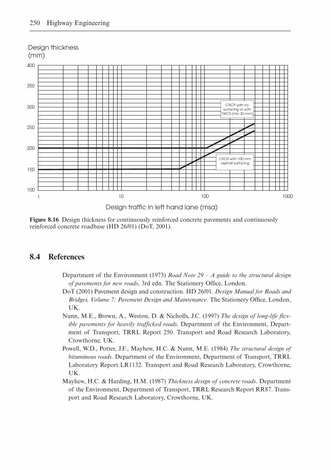
8.4 References
Department of the Environment (1973) Road Note 29 – A guide to the structural designof pavements for new roads, 3rd edn. The Stationery Office, London.
DoT (2001) Pavement design and construction. HD 26/01. Design Manual for Roads andBridges, Volume 7: Pavement Design and Maintenance. The Stationery Office, London,UK.
Nunn, M.E., Brown, A., Weston, D. & Nicholls, J.C. (1997) The design of long-life flex-ible pavements for heavily trafficked roads. Department of the Environment, Depart-ment of Transport, TRRL Report 250. Transport and Road Research Laboratory,Crowthorne, UK.
Powell, W.D., Potter, J.F., Mayhew, H.C. & Nunn, M.E. (1984) The structural design ofbituminous roads. Department of the Environment, Department of Transport, TRRLLaboratory Report LR1132. Transport and Road Research Laboratory, Crowthorne,UK.
Mayhew, H.C. & Harding, H.M. (1987) Thickness design of concrete roads. Departmentof the Environment, Department of Transport, TRRL Research Report RR87. Trans-port and Road Research Laboratory, Crowthorne, UK.
250 Highway Engineering
Design traffic in left hand lane (msa)
Design thickness(mm)
1000 100 10 1
100
150
200
250
300
350
400
CRCR with 100 mm asphalt surfacing
CRCP with no surfacing or with
TWCS (min 30 mm)
Figure 8.16 Design thickness for continuously reinforced concrete pavements and continuouslyreinforced concrete roadbase (HD 26/01) (DoT, 2001).
Chapter 9
Pavement Maintenance
9.1 Introduction
Highway pavements, once constructed, will not last forever. After a time, signsof wear will appear. These signs include cracking, rutting and polishing of theroad’s surface. A point will arrive where the wear and tear is at such an advancedstage that the integrity of the pavement and hence the standard of service pro-vided by it has diminished. Maintenance is required at this point to prolong thehighway’s useful life. Loss of skidding resistance and loss of texture are formsof deterioration eventually suffered by all highway pavements.
In order to carry out the maintenance in as cost-effective a manner as possi-ble, a logical coherent procedure must be adopted in order to select the mosteffective form that the maintenance should take, together with the optimum timeat which this work should be undertaken. Minor maintenance may be sufficientto maintain the required standard of service for the motorist. However, in situ-ations where major structural strengthening is required, a comprehensive struc-tural investigation is vital in order to assist in the completion of the requireddetailed design (HD 30/99) (DoT, 1999).
9.2 Forms of maintenance
For bituminous roads, maintenance can be either minor or major. Minor main-tenance takes the form of patching. It allows defective materials, particularlythose in the surface courses of the pavement, to be replaced. If done properly,it can restore the stability and riding quality of the surface, arresting its deteri-oration and extending its serviceable life. It is an integral part of highway main-tenance and makes sound economic sense.
Patching can remedy the following defects:
� Substandard drainage or some other problem related to the subgrade whichwill cause the failure of the pavement’s foundation
� The aging of the bituminous surface, causing its break-up with the conse-quent formation of potholes and areas of crazing
� Decreased load bearing capacity of the pavement due to the ingress of waterand damage due to frost.
Patching involves the repair of random areas of substandard pavement, not continuous widths/lengths.
Major maintenance of bituminous pavements may involve removing all orpart of the surface using a planer and resurfacing the road, or laying a layer ofbitumen over the existing one. The process of overlaying is dealt with in detailwithin this text as bituminous pavements are designed under LR1132 on thebasis that, at the end of their design life, their structural integrity is such thatthe application of an overlay will significantly extend their useful life.
Both overlaying and resurfacing are carried out for the following commonreasons (HD 31/94) (DoT, 1994c):
� To strengthen the highway pavement� To replace defective materials� To restore skidding resistance� To improve riding quality.
Design of an overlay (minimum 50mm thick) involves estimating the thicknessrequired to deliver the required additional life to the pavement slab.
For concrete pavements, maintenance can take the following forms:
� Surface treatment – having assessed the skidding resistance of the pavement(using SCRIM – see section 9.7), it can be restored to an acceptable level bymethods such as surface dressing consisting of epoxy resin-based binder andcalcined bauxite chippings or mechanical roughening of the worn concretesurfacing by abrasive blasting or scabbling.
� Joint repairs – defective joint seals allow foreign matter to enter between theslabs and penetrate the lower levels of the pavement. Replacement of theseal will rectify this defect.
� Structural repair – cracks in the slab or movement at the joints can lead tooutright failure if not treated. These are defined in terms of increasing sever-ity as narrow (less than 0.5mm), medium (between 0.5mm and 1.5mm) orwide (greater than 1.5mm). Narrow cracks generally require no immediateaction, but may require to be sealed. Medium cracks require a groove to beformed and a seal to be applied, while wide cracks may require a full-depthrepair or bay replacement.
� Strengthening – may be required in order to extend the pavement’s life dueto increased traffic levels or because the slab in its present unimproved stateis unable to carry the traffic predicted. This is accomplished using overlays.This is a more difficult process than for bituminous pavements due to theexistence of joints. Therefore, concrete overlays are carried out either byforming joints in the overlay at the same location as those underneath or byseparating the two concrete layers using a regulating layer of bituminousmaterial. If a bitumen-based overlay is used, added thickness may be
252 Highway Engineering
required to deal not only with the structural requirements of the slab butalso to counteract reflection cracking resulting from movements in the jointswithin the underlying concrete slab (HD 32/94) (DoT, 1994d).
9.3 Compiling information on the pavement’s condition
An inventory of highway condition data is updated on a routinely regular basisin order to determine the condition of the pavement and whether its level ofdeterioration is such that remedial action is necessary. The data compiled willallow trends in the structural condition of a pavement to be established.
The four major types of routine assessment are (HD 30/99) (DoT, 1999):
� Visual condition surveys� High speed road monitor� Deflectograph� SCRIM (see section 9.7).
The first three are dealt with here, and the fourth later in the chapter.
Visual condition surveys
These record defects that remain undetected by machine-based methods. As themethod is slow and laborious, it is usually targeted on specific areas in particu-larly poor condition. The surveys provide factual information for deciding onthe most appropriate structural treatments, and identify sections of highwaysuitable for remedial treatment. Planning for long-term treatment can thus beundertaken, with performance of the pavements being monitored and prioritiesfor treatment being established on the basis of the database compiled.
In past times a Marshall Survey represented the usual method for preparingan inventory of the condition of sections of highway. It involved groups of tech-nical staff compiling information throughout their area on the condition ofcarriageways, kerbs, etc. Nowadays, the information can be collated using thecomputer program CHART (Computerised Highway Assessment of Ratingsand Treatments), a management system for assisting maintenance engineers. Itprovides information on the lengths of highway that are substandard, the treat-ments required and the relative priorities for treatment.
For every 100-metre section of highway, CHART convert defects informationinto numerical ratings for each existing defect. Those defects requiring treatmentcan then be identified. The ratings, which are subjectively based, indicate therelative urgency of the need for treatment.
Typical output is:
Map CHART – the quantity of defects are shown by chainage both along andacross the highway
Pavement Maintenance 253
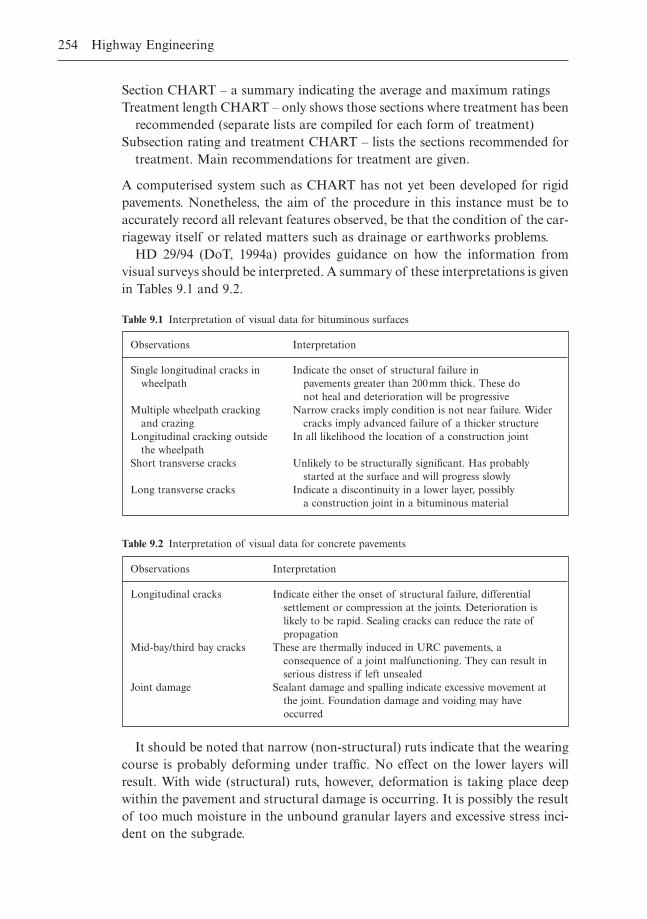
Section CHART – a summary indicating the average and maximum ratingsTreatment length CHART – only shows those sections where treatment has been
recommended (separate lists are compiled for each form of treatment)Subsection rating and treatment CHART – lists the sections recommended for
treatment. Main recommendations for treatment are given.
A computerised system such as CHART has not yet been developed for rigidpavements. Nonetheless, the aim of the procedure in this instance must be toaccurately record all relevant features observed, be that the condition of the car-riageway itself or related matters such as drainage or earthworks problems.
HD 29/94 (DoT, 1994a) provides guidance on how the information fromvisual surveys should be interpreted. A summary of these interpretations is givenin Tables 9.1 and 9.2.
254 Highway Engineering
Observations Interpretation
Single longitudinal cracks in Indicate the onset of structural failure inwheelpath pavements greater than 200mm thick. These do
not heal and deterioration will be progressiveMultiple wheelpath cracking Narrow cracks imply condition is not near failure. Wider
and crazing cracks imply advanced failure of a thicker structureLongitudinal cracking outside In all likelihood the location of a construction joint
the wheelpathShort transverse cracks Unlikely to be structurally significant. Has probably
started at the surface and will progress slowlyLong transverse cracks Indicate a discontinuity in a lower layer, possibly
a construction joint in a bituminous material
Table 9.1 Interpretation of visual data for bituminous surfaces
Observations Interpretation
Longitudinal cracks Indicate either the onset of structural failure, differential settlement or compression at the joints. Deterioration is likely to be rapid. Sealing cracks can reduce the rate ofpropagation
Mid-bay/third bay cracks These are thermally induced in URC pavements, a consequence of a joint malfunctioning. They can result in serious distress if left unsealed
Joint damage Sealant damage and spalling indicate excessive movement at the joint. Foundation damage and voiding may have occurred
Table 9.2 Interpretation of visual data for concrete pavements
It should be noted that narrow (non-structural) ruts indicate that the wearingcourse is probably deforming under traffic. No effect on the lower layers willresult. With wide (structural) ruts, however, deformation is taking place deepwithin the pavement and structural damage is occurring. It is possibly the resultof too much moisture in the unbound granular layers and excessive stress inci-dent on the subgrade.
High speed road monitor
The high speed road monitor (HRM) measures parameters such as ridingquality, texture and rutting. It consists of a van and 4.5 metre-long trailer fittedwith four laser sensors along the nearside wheelpath. It allows the condition ofthe highway’s surface to be assessed under conditions of normal traffic withspeeds up to 95km/h.
HRM is not designed to replace other slower visual techniques, but will allowthem to be more effectively used by targeting them on the more vulnerable sections of pavement as identified by this methodology.
The four lasers within the HRM provide data on the longitudinal profile andmacrotexture of the pavement. In addition, a laser mounted at the mid-point ofthe trailer axle is used along with the trailer wheels to measure the average rutdepth in the nearside and offside wheelpaths. Inclinometers mounted on thetrailer estimate the crossfall and gradient on the highway. Horizontal radius ofcurvature can also be estimated. A device fitted to the nearside trailer wheel pro-vides distance information to which all HRM measurements are referenced.
The following major parameters are measured within HRM:
� Longitudinal profile – profile unevenness is used to assess riding quality forthe road user. It measures deviations away from a moving datum which represents an average profile along the highway
� Rutting – HRM records the average rut depth to the nearside and offsidewheelpaths
� Macrotexture – this is the coarser element of the surfacing, formed either bythe aggregate particles in the surfacing or grooves in the concrete surface. Itcontributes to skidding resistance, particularly at high speeds, mainly by providing drainage paths for the water
� Alignment parameters – gradient, crossfall and radius of curvature mea-surements are estimated to an accuracy of ±10%.
HRM surveys are only beginning to be used on a routine basis. Results fromthem should be used for general guidance only. Its main function is to identifyspecific discrete locations where more established but more costly and time con-suming methods of analysis should be used.
Deflection beam/deflectograph
The deflection beam is a widely accepted instrument for assessing the structuralcondition of flexible highway surfacings. Originated by Dr A.C. Benkleman anddeveloped by the Transport Research Laboratory (Kennedy et al., 1978a), itinvolves applying a load to the pavement’s surface and monitoring its conse-quent vertical deflection. As a loaded wheel passes over the pavement surface,the deflection of the slab is measured by the rotation of a long pivoted beamtouching the surface at the point where the deflection is to be determined. The
Pavement Maintenance 255
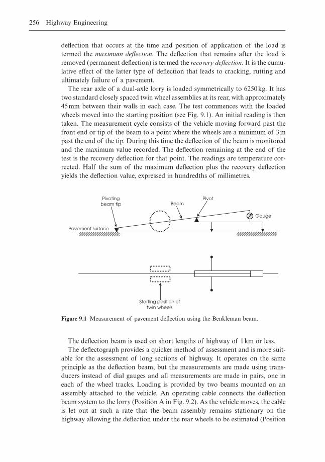
deflection that occurs at the time and position of application of the load istermed the maximum deflection. The deflection that remains after the load isremoved (permanent deflection) is termed the recovery deflection. It is the cumu-lative effect of the latter type of deflection that leads to cracking, rutting andultimately failure of a pavement.
The rear axle of a dual-axle lorry is loaded symmetrically to 6250kg. It hastwo standard closely spaced twin wheel assemblies at its rear, with approximately45mm between their walls in each case. The test commences with the loadedwheels moved into the starting position (see Fig. 9.1). An initial reading is thentaken. The measurement cycle consists of the vehicle moving forward past thefront end or tip of the beam to a point where the wheels are a minimum of 3mpast the end of the tip. During this time the deflection of the beam is monitoredand the maximum value recorded. The deflection remaining at the end of thetest is the recovery deflection for that point. The readings are temperature cor-rected. Half the sum of the maximum deflection plus the recovery deflectionyields the deflection value, expressed in hundredths of millimetres.
256 Highway Engineering
Pavement surface
Pivoting beam tip Beam
Pivot
Gauge
Starting position of twin wheels
Figure 9.1 Measurement of pavement deflection using the Benkleman beam.
The deflection beam is used on short lengths of highway of 1km or less.The deflectograph provides a quicker method of assessment and is more suit-
able for the assessment of long sections of highway. It operates on the sameprinciple as the deflection beam, but the measurements are made using trans-ducers instead of dial gauges and all measurements are made in pairs, one ineach of the wheel tracks. Loading is provided by two beams mounted on anassembly attached to the vehicle. An operating cable connects the deflectionbeam system to the lorry (Position A in Fig. 9.2). As the vehicle moves, the cableis let out at such a rate that the beam assembly remains stationary on thehighway allowing the deflection under the rear wheels to be estimated (Position
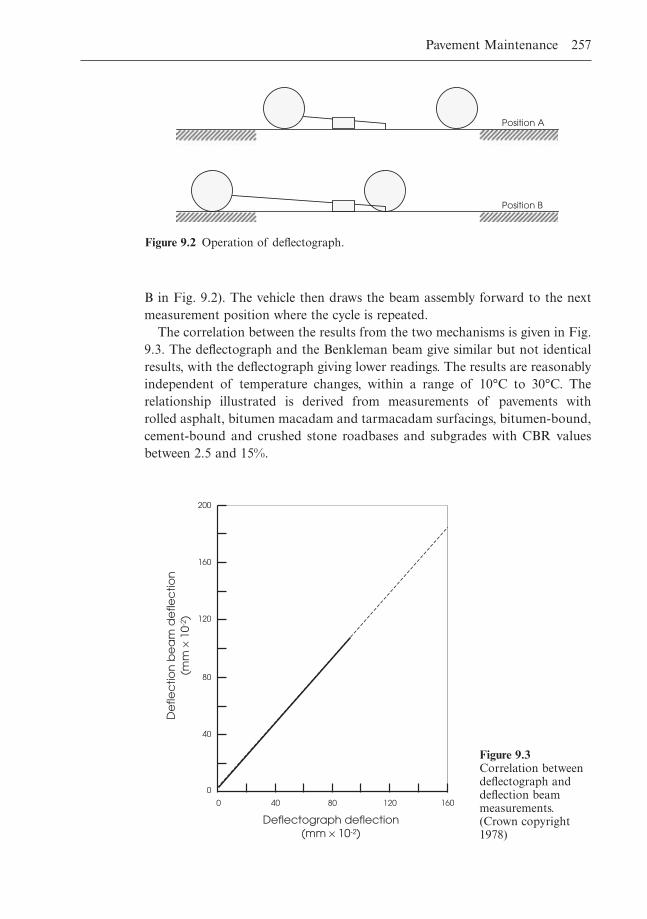
B in Fig. 9.2). The vehicle then draws the beam assembly forward to the nextmeasurement position where the cycle is repeated.
The correlation between the results from the two mechanisms is given in Fig.9.3. The deflectograph and the Benkleman beam give similar but not identicalresults, with the deflectograph giving lower readings. The results are reasonablyindependent of temperature changes, within a range of 10°C to 30°C. The relationship illustrated is derived from measurements of pavements with rolled asphalt, bitumen macadam and tarmacadam surfacings, bitumen-bound,cement-bound and crushed stone roadbases and subgrades with CBR valuesbetween 2.5 and 15%.
Pavement Maintenance 257
Position A
Position B
Figure 9.2 Operation of deflectograph.
Deflectograph deflection (mm ¥ 10-2)
200
160
120
80
40
40 80 120 160 0
0
De
flec
tion
be
am
de
flec
tion
(m
m ¥
10-
2 )
Figure 9.3Correlation betweendeflectograph anddeflection beammeasurements.(Crown copyright1978)
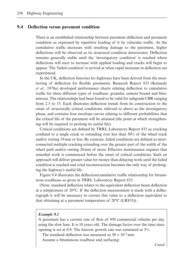
9.4 Deflection versus pavement condition
There is an established relationship between pavement deflection and pavementcondition as expressed by repetitive loading of it by vehicular traffic. As thecumulative traffic increases with resulting damage to the pavement, higherdeflections will be observed as its structural condition deteriorates. Deflectionremains generally stable until the ‘investigatory condition’ is reached wheredeflections will start to increase with applied loading and cracks will begin toappear. The ‘failed condition’ is arrived at when rapid increases in deflection areexperienced.
In the UK, deflection histories for highways have been derived from the mon-itoring of deflection for flexible pavements. Research Report 833 (Kennedy et al., 1978a) developed performance charts relating deflection to cumulativetraffic for three different types of roadbase: granular, cement bound and bitu-minous. The relationships had been found to be valid for subgrade CBR rangingfrom 2.5 to 15. Each illustrates deflection trends from its construction to theonset of structurally critical conditions, referred to above as the investigatoryphase, and contains four envelope curves relating to different probabilities thatthe critical life of the pavement will be attained (the point at which strengthen-ing will be required to prolong its useful life).
Critical conditions are defined by TRRL Laboratory Report 833 as crackingconfined to a single crack or extending over less than 50% of the wheel trackand/or rutting 19mm or less. By contrast, failed conditions are defined as inter-connected multiple cracking extending over the greater part of the width of thewheel path and/or rutting 20mm of more. Effective maintenance requires thatremedial work is commenced before the onset of critical conditions. Such anapproach will deliver greater value for money than delaying work until the failedcondition is reached and total reconstruction becomes the only way of prolong-ing the highway’s useful life.
Figure 9.4 illustrates the deflection/cumulative traffic relationship for bitumi-nous roadbases as given in TRRL Laboratory Report 833.
(Note: standard deflection relates to the equivalent deflection beam deflectionat a temperature of 20°C. If the deflection measurement is made with a deflec-tograph it will be necessary to correct this value to a deflection equivalent tothat obtaining at a pavement temperature of 20°C (LR833)).
258 Highway Engineering
Example 9.1A pavement has a current rate of flow of 950 commercial vehicles per dayusing the slow lane. It is 10 years old. The damage factor over the time sinceopening is set at 0.9. The historic growth rate was estimated at 3%.
The standard deflection was measured as 50 ¥ 10-2 mm.Assume a bituminous roadbase and surfacing:
Contd
Pavement Maintenance 259
Example 9.1 Contd
(1) Estimate the life in millions of standard axles that the pavement has a0.5 probability of achieving
(2) Estimate the life in millions of standard axles that the pavement has a0.9 probability of achieving.
Solution
If the daily flow of commercial vehicles after 10 years is 950 vehicles, then,assuming a growth rate of 3%, the initial flow on the opening day is esti-mated using the following formula:
F0 = Fn/(1 + r)n
whereF0 = initial flow on opening dayFn = flow after n yearsr = traffic growth rate
Substituting the above values into Equation 9.1, the following initial flow isobtained:
F0 = 950/(1.03)10
= 706.89 commercial vehicles
Addis and Robinson (1983) have shown that the total number of commer-cial vehicles Tn, using the slow lane over a given time span n can be expressedin terms of the initial daily flow F0, the growth rate r as follows:
Tn = 365F0 /((1 + r)n - 1)/r)
Therefore, since:
F0 = 706.89r = 0.03n = 10
Tn = (365 ¥ 706.89)/((1.03)10 - 1)/0.03)= 2.96 million commercial vehicles
This figure multiplied by the historic vehicle damage factor gives the totalnumber of standard axles incident on the pavement since its opening:
Cumulative standard axles = 2.96 ¥ 0.9 = 2.66 million standard axles (msa)
From Fig. 9.4, it can be seen that a pavement with a bituminous roadbaseand a standard deflection of 50 ¥ 10-2 mm has a 0.5 probability of achieving
Contd
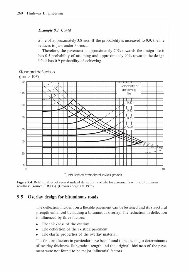
9.5 Overlay design for bituminous roads
The deflection incident on a flexible pavement can be lessened and its structuralstrength enhanced by adding a bituminous overlay. The reduction in deflectionis influenced by three factors:
� The thickness of the overlay� The deflection of the existing pavement� The elastic properties of the overlay material.
The first two factors in particular have been found to be the major determinantsof overlay thickness. Subgrade strength and the original thickness of the pave-ment were not found to be major influential factors.
260 Highway Engineering
Example 9.1 Contd
a life of approximately 3.8msa. If the probability is increased to 0.9, the lifereduces to just under 3.0msa.
Therefore, the pavement is approximately 70% towards the design life ithas 0.5 probability of attaining and approximately 90% towards the designlife it has 0.9 probability of achieving.
4010 10.1 0
20
40
60
80
100
120
Cumulative standard axles (msa)
Standard deflection (mm ¥ 10-2) 140
Probability of achieving
life
0.25
0.50
0.75
0.90
Figure 9.4 Relationship between standard deflection and life for pavements with a bituminousroadbase (source: LR833). (Crown copyright 1978)
Within this text, an empirical overlay design method for flexible pavements as detailed in LR833 is presented. Other methods such as component analy-sis (Asphalt Institute, 1983) and analytically based processes (Claessen & Ditmarsch, 1977) are also available but are not addressed here.
The information in LR833 is based on the results of full-scale highway experi-ments where the surface has been overlaid with rolled asphalt at a time when,some sections of the road were approaching failure.
The LR833 method is based on assigning a representative deflection to asection of highway – termed the 85th percentile value (85% of the deflectionsfound are less than this value). This value is then used in association with thefamily of curves as given in Fig. 9.4 to deliver a predicted life. If this is less thanrequired, a bituminous overlay can be considered. Any residual life derived willbe the period of time remaining before the application of an overlay or someother form of remedial action will be necessary.
The overlay design procedure is contained within a number of charts, eachspecifying the thickness of rolled asphalt overlay required to strengthen a pave-ment of given deflection so that the extended life required by the designer canbe achieved. Charts for four different roadbases are contained in LR833:
� Granular roadbases whose aggregates have a natural cementing action� Non-cementing granular roadbases� Cement-bound roadbases� Bituminous roadbases.
For a given roadbase material, different overlay thicknesses will be deriveddepending on the probability assigned to the assessment of the remaining lifeof an existing pavement and to the design of the extension of its life by over-laying. Therefore, LR833 supplies design charts for two different levels of prob-ability, 0.5 and 0.9, for each roadbase material.
An illustration of the design chart for bituminous roadbases with a 0.5 prob-ability of achieving their desired life is given in Fig. 9.5.
Pavement Maintenance 261
Example 9.2 – Overlay design using LR833Taking the pavement detailed in Example 9.1. If a further 15 years of serviceis required from the pavement and the vehicle damage factor is expected tobe 1.05 over this time span, estimate the thickness of bituminous overlayrequired to provide sufficient strengthening.
The future growth rate for traffic is set at 4%. Assume a 0.5 probabilitylevel.
Solution
Assuming that the present flow is 950 vehicles per day, using Equation 9.2,the estimation of cumulative traffic over the next 15 years is:
Tn = 365F0 /((1 + r)n - 1)/r)Contd
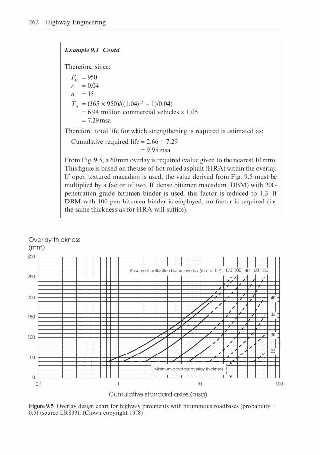
262 Highway Engineering
Example 9.1 Contd
Therefore, since:
F0 = 950r = 0.04n = 15
Tn = (365 ¥ 950)/((1.04)15 - 1)/0.04)= 6.94 million commercial vehicles ¥ 1.05= 7.29msa
Therefore, total life for which strengthening is required is estimated as:
Cumulative required life = 2.66 + 7.29= 9.95msa
From Fig. 9.5, a 60mm overlay is required (value given to the nearest 10mm).This figure is based on the use of hot rolled asphalt (HRA) within the overlay.If open textured macadam is used, the value derived from Fig. 9.5 must bemultiplied by a factor of two. If dense bitumen macadam (DBM) with 200-penetration grade bitumen binder is used, this factor is reduced to 1.3. IfDBM with 100-pen bitumen binder is employed, no factor is required (i.e.the same thickness as for HRA will suffice).
Cumulative standard axles (msa)
Overlay thickness (mm)
100 10 1 0.1
0
50
100
150
200
250
300
Minimum practical overlay thickness
Pavement deflection before overlay (mm × 10–2): 120 100 80 60 50
40
35
30
25
Figure 9.5 Overlay design chart for highway pavements with bituminous roadbases (probability =0.5) (source LR833). (Crown copyright 1978)
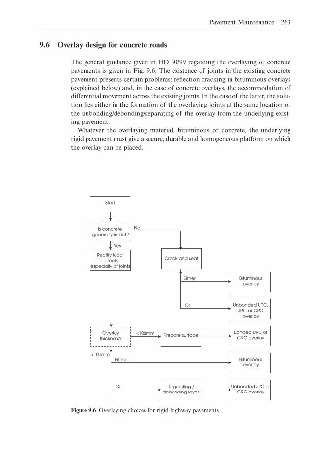
9.6 Overlay design for concrete roads
The general guidance given in HD 30/99 regarding the overlaying of concretepavements is given in Fig. 9.6. The existence of joints in the existing concretepavement presents certain problems: reflection cracking in bituminous overlays(explained below) and, in the case of concrete overlays, the accommodation ofdifferential movement across the existing joints. In the case of the latter, the solu-tion lies either in the formation of the overlaying joints at the same location orthe unbonding/debonding/separating of the overlay from the underlying exist-ing pavement.
Whatever the overlaying material, bituminous or concrete, the underlyingrigid pavement must give a secure, durable and homogeneous platform on whichthe overlay can be placed.
Pavement Maintenance 263
Crack and seat
Bituminous overlay
Unbonded URC, JRC or CRC
overlay
Bonded URC or CRC overlay
Bituminous overlay
Unbonded JRC or CRC overlay
Start
Is concrete
generally intact?
Rectify local defects,
especially at joints
Overlay thickness?
Prepare surface
Regulating / debonding layer
No
Yes
Either
Or
<100mm
>100mm Either
Or
Figure 9.6 Overlaying choices for rigid highway pavements.
9.6.1 Bitumen-bound overlays placed over rigid pavements
For unreinforced and reinforced jointed pavements (URC and JRC), the overlaythickness may be controlled by the need to either reduce or delay the onset ofreflection cracking rather than for basic structural reasons. Reflection crackingarises where the cracking pattern in the underlying pavement ‘comes through’the overlay giving a similarly shaped pattern on the surface. A 180mm thickoverlay is usually required to counteract this condition.
If existing pavements have deteriorated markedly, it may be appropriate to‘crack and seal’ before overlaying. This preliminary procedure involves induc-ing fine vertical transverse cracks in the existing concrete pavement, therebyreducing the load distributing properties of the slab but assisting in the con-trolling of reflection cracking.
9.6.2 Concrete overlays
Concrete overlays are not widely used within the UK (HD 30/99). This treat-ment results in the existing pavement having a longer life and improved surfacecharacteristics as well as providing improved strength characteristics. A concreteoverlay will function better if the existing pavement slab beneath it provides agood, firm foundation. Use of a thick concrete overlay is not suitable where theexisting foundation is in a poor condition and where indications are that thesubgrade is weak, in which case reconstruction may be the only viable option(HD 30/99). For a concrete overlay to be successfully used, it is imperative thatthe foundation is in good condition. Any voiding beneath a rigid slab should befilled with grout. In the case of a flexible/flexible composite pavement, any cracksshould be repaired to ensure a good supporting structure.
Accurate information on the structural condition of the original pavementstructure is required in order to make optimum use of the concrete overlaydesign method. The equivalent surface foundation modulus (ESFM) is the vari-able most often used to state, in quantitative terms, the structural integrity ofthe foundation.
Equivalent surface foundation modulus (ESFM)
This modulus was outlined in RR 87 (Mayhew & Harding, 1987). It evaluatesthe support offered by the foundation to a concrete pavement slab in terms ofYoung’s modulus of an equivalent uniform elastic foundation of infinite depth.Equivalence is defined within RR 87 as ‘the uniform elastic foundation with thesame surface deflection, under a standard wheel load, as that of the actual foun-dation’. Equivalent thickness is thus used to transform the foundation into acorresponding single layer supported on a uniform elastic medium. Use of
264 Highway Engineering
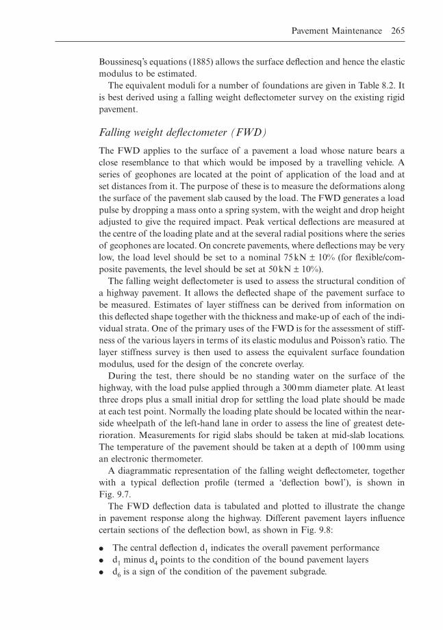
Boussinesq’s equations (1885) allows the surface deflection and hence the elasticmodulus to be estimated.
The equivalent moduli for a number of foundations are given in Table 8.2. Itis best derived using a falling weight deflectometer survey on the existing rigidpavement.
Falling weight deflectometer (FWD)
The FWD applies to the surface of a pavement a load whose nature bears aclose resemblance to that which would be imposed by a travelling vehicle. Aseries of geophones are located at the point of application of the load and atset distances from it. The purpose of these is to measure the deformations alongthe surface of the pavement slab caused by the load. The FWD generates a loadpulse by dropping a mass onto a spring system, with the weight and drop heightadjusted to give the required impact. Peak vertical deflections are measured atthe centre of the loading plate and at the several radial positions where the seriesof geophones are located. On concrete pavements, where deflections may be verylow, the load level should be set to a nominal 75kN ± 10% (for flexible/com-posite pavements, the level should be set at 50kN ± 10%).
The falling weight deflectometer is used to assess the structural condition ofa highway pavement. It allows the deflected shape of the pavement surface tobe measured. Estimates of layer stiffness can be derived from information onthis deflected shape together with the thickness and make-up of each of the indi-vidual strata. One of the primary uses of the FWD is for the assessment of stiff-ness of the various layers in terms of its elastic modulus and Poisson’s ratio. Thelayer stiffness survey is then used to assess the equivalent surface foundationmodulus, used for the design of the concrete overlay.
During the test, there should be no standing water on the surface of thehighway, with the load pulse applied through a 300mm diameter plate. At leastthree drops plus a small initial drop for settling the load plate should be madeat each test point. Normally the loading plate should be located within the near-side wheelpath of the left-hand lane in order to assess the line of greatest dete-rioration. Measurements for rigid slabs should be taken at mid-slab locations.The temperature of the pavement should be taken at a depth of 100mm usingan electronic thermometer.
A diagrammatic representation of the falling weight deflectometer, togetherwith a typical deflection profile (termed a ‘deflection bowl’), is shown in Fig. 9.7.
The FWD deflection data is tabulated and plotted to illustrate the change in pavement response along the highway. Different pavement layers influencecertain sections of the deflection bowl, as shown in Fig. 9.8:
� The central deflection d1 indicates the overall pavement performance� d1 minus d4 points to the condition of the bound pavement layers� d6 is a sign of the condition of the pavement subgrade.
Pavement Maintenance 265
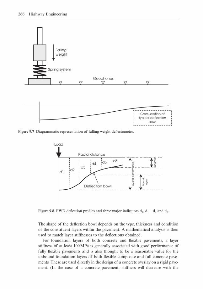
The shape of the deflection bowl depends on the type, thickness and conditionof the constituent layers within the pavement. A mathematical analysis is thenused to match layer stiffnesses to the deflections obtained.
For foundation layers of both concrete and flexible pavements, a layer stiffness of at least 100MPa is generally associated with good performance offully flexible pavements and is also thought to be a reasonable value for theunbound foundation layers of both flexible composite and full concrete pave-ments. These are used directly in the design of a concrete overlay on a rigid pave-ment. (In the case of a concrete pavement, stiffness will decrease with the
266 Highway Engineering
Falling weight
Spring system
Geophones
Cross-section of typical deflection
bowl
Figure 9.7 Diagrammatic representation of falling weight deflectometer.
d1 d2 d3
d4 d5 d6
Load
Radial distance
Deflection bowl Ove
rall
pe
rfo
rma
nc
e
Bou
nd
la
yers
Sub
gra
de
Figure 9.8 FWD deflection profiles and three major indicators d1, d1 - d4 and d6.
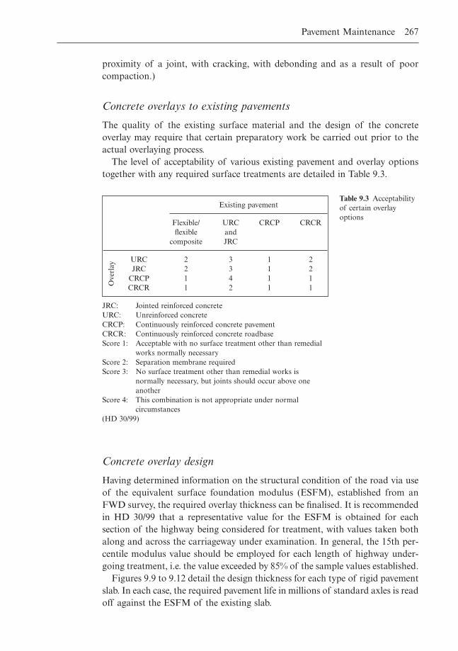
proximity of a joint, with cracking, with debonding and as a result of poor compaction.)
Concrete overlays to existing pavements
The quality of the existing surface material and the design of the concreteoverlay may require that certain preparatory work be carried out prior to theactual overlaying process.
The level of acceptability of various existing pavement and overlay optionstogether with any required surface treatments are detailed in Table 9.3.
Pavement Maintenance 267
Ove
rlay
Existing pavement
Flexible/ URC CRCP CRCRflexible and
composite JRC
URC 2 3 1 2JRC 2 3 1 2
CRCP 1 4 1 1CRCR 1 2 1 1
Table 9.3 Acceptabilityof certain overlayoptions
JRC: Jointed reinforced concreteURC: Unreinforced concreteCRCP: Continuously reinforced concrete pavementCRCR: Continuously reinforced concrete roadbaseScore 1: Acceptable with no surface treatment other than remedial
works normally necessaryScore 2: Separation membrane required Score 3: No surface treatment other than remedial works is
normally necessary, but joints should occur above oneanother
Score 4: This combination is not appropriate under normalcircumstances
(HD 30/99)
Concrete overlay design
Having determined information on the structural condition of the road via useof the equivalent surface foundation modulus (ESFM), established from anFWD survey, the required overlay thickness can be finalised. It is recommendedin HD 30/99 that a representative value for the ESFM is obtained for eachsection of the highway being considered for treatment, with values taken bothalong and across the carriageway under examination. In general, the 15th per-centile modulus value should be employed for each length of highway under-going treatment, i.e. the value exceeded by 85% of the sample values established.
Figures 9.9 to 9.12 detail the design thickness for each type of rigid pavementslab. In each case, the required pavement life in millions of standard axles is readoff against the ESFM of the existing slab.
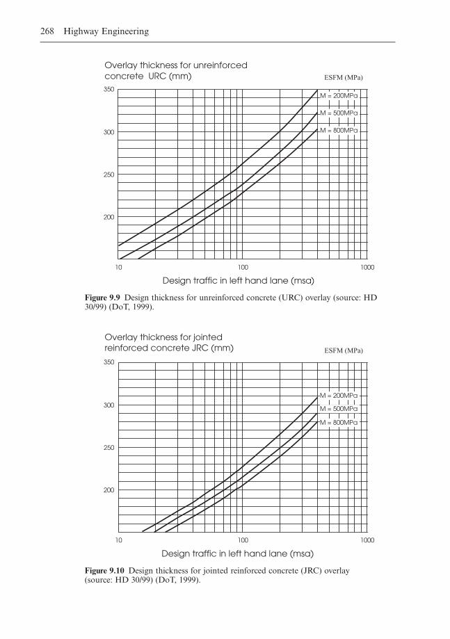
268 Highway Engineering
Overlay thickness for unreinforced concrete URC (mm)
Design traffic in left hand lane (msa)
350
300
250
200
10 100 1000
ESFM (MPa)
M = 200MPa
M = 500MPa
M = 800MPa
Figure 9.9 Design thickness for unreinforced concrete (URC) overlay (source: HD30/99) (DoT, 1999).
Overlay thickness for jointed reinforced concrete JRC (mm)
350
300
250
200
10 100 1000
Design traffic in left hand lane (msa)
ESFM (MPa)
M = 200MPa
M = 500MPa
M = 800MPa
Figure 9.10 Design thickness for jointed reinforced concrete (JRC) overlay (source: HD 30/99) (DoT, 1999).
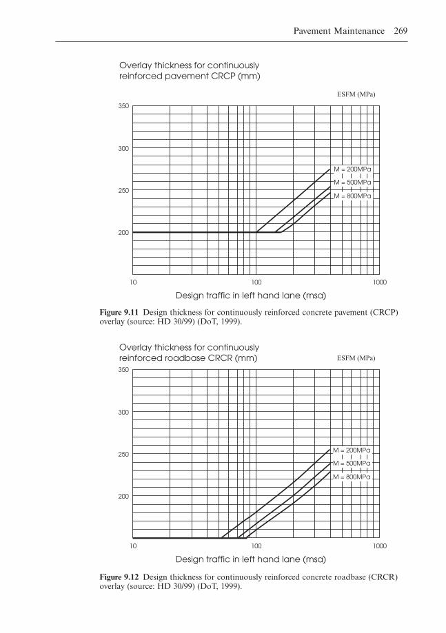
Pavement Maintenance 269
350
300
250
200
10 100 1000
Design traffic in left hand lane (msa)
ESFM (MPa)
Overlay thickness for continuously reinforced pavement CRCP (mm)
M = 200MPa
M = 500MPa
M = 800MPa
Overlay thickness for continuously reinforced roadbase CRCR (mm)350
300
250
200
10 100 1000
Design traffic in left hand lane (msa)
ESFM (MPa)
M = 200MPa
M = 500MPa
M = 800MPa
Figure 9.11 Design thickness for continuously reinforced concrete pavement (CRCP)overlay (source: HD 30/99) (DoT, 1999).
Figure 9.12 Design thickness for continuously reinforced concrete roadbase (CRCR)overlay (source: HD 30/99) (DoT, 1999).
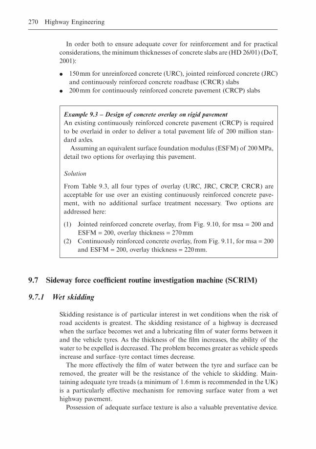
In order both to ensure adequate cover for reinforcement and for practicalconsiderations, the minimum thicknesses of concrete slabs are (HD 26/01) (DoT,2001):
� 150mm for unreinforced concrete (URC), jointed reinforced concrete (JRC)and continuously reinforced concrete roadbase (CRCR) slabs
� 200mm for continuously reinforced concrete pavement (CRCP) slabs
270 Highway Engineering
Example 9.3 – Design of concrete overlay on rigid pavementAn existing continuously reinforced concrete pavement (CRCP) is requiredto be overlaid in order to deliver a total pavement life of 200 million stan-dard axles.
Assuming an equivalent surface foundation modulus (ESFM) of 200MPa,detail two options for overlaying this pavement.
Solution
From Table 9.3, all four types of overlay (URC, JRC, CRCP, CRCR) areacceptable for use over an existing continuously reinforced concrete pave-ment, with no additional surface treatment necessary. Two options areaddressed here:
(1) Jointed reinforced concrete overlay, from Fig. 9.10, for msa = 200 andESFM = 200, overlay thickness = 270mm
(2) Continuously reinforced concrete overlay, from Fig. 9.11, for msa = 200and ESFM = 200, overlay thickness = 220mm.
9.7 Sideway force coefficient routine investigation machine (SCRIM)
9.7.1 Wet skidding
Skidding resistance is of particular interest in wet conditions when the risk ofroad accidents is greatest. The skidding resistance of a highway is decreasedwhen the surface becomes wet and a lubricating film of water forms between itand the vehicle tyres. As the thickness of the film increases, the ability of thewater to be expelled is decreased. The problem becomes greater as vehicle speedsincrease and surface–tyre contact times decrease.
The more effectively the film of water between the tyre and surface can beremoved, the greater will be the resistance of the vehicle to skidding. Main-taining adequate tyre treads (a minimum of 1.6mm is recommended in the UK)is a particularly effective mechanism for removing surface water from a wethighway pavement.
Possession of adequate surface texture is also a valuable preventative device.
The texture depth or ‘macrotexture’ of the surface refers to the general profileof, and gaps in between, the channels/grooves in the road surfacing. It con-tributes to skidding resistance, primarily at high speeds, both by providingdrainage paths that allow the water to be removed from the tyre/road interfaceand by the presence of projections that contribute to hysteresis losses in the tyre(this relates to a tyre’s capability to deform in shape around the particles of theaggregate within the surfacing, causing a consequent loss of energy). The sandpatch test is the oldest method for measuring texture depth. It involves using aknown volume of sand to fill the voids in the pavement surface up to their peaks,measuring the surface area covered by the sand and calculating the texture depthby dividing the volume of sand by the area of the patch.
The microscopic texture of the aggregate in the surfacing material is alsocrucial to skidding resistance. Termed ‘microtexture’, it relates to the aggregate’sphysical properties and is important to low-speed skidding resistance. Morerounded, smooth particles offer less resistance to skidding than rougher con-stituents. The action of traffic will tend gradually to reduce a particle’s micro-texture. Its susceptibility to this wearing action is measured by the parameterpolished stone value (PSV). First introduced in the UK in the 1950s, the PSVtest is the only standard laboratory method of microtexture measurement withinthe UK (Roe & Hartshorne, 1998). It is a measure of the long-term frictionalproperty of the microtexture.
The test is performed in two parts. First, cubic-shaped, slightly curved, 10mmtest specimens are placed in an accelerated polishing machine, where they aresubject to polishing/abrasion for 6 hours. Second, a pendulum friction testermeasures the degree to which the specimens have been polished. The result gen-erally lies in the 30 to 80 range, with higher values indicating higher resistanceto polishing.
Chippings utilised within a hot rolled asphalt wearing course or as part of asurface dressing process must possess a minimum PSV valuation, depending onthe type of site (approach to traffic signal, roundabout, link road) and the dailytraffic flows. Sensitive junction locations usually require surfacing materials tohave a PSV in the 65 to 75 range, with a general minimum value of 45 requiredat non-critical locations.
9.7.2 Using SCRIM
As noted earlier in the chapter, SCRIM constitutes a major form of routineassessment of a highway’s condition. It measures the skidding resistance of thehighway surface that is being gradually reduced by the polishing action of thevehicular traffic (DoT, 1994a).
A vehicle will skid whenever the available friction between the road surfaceand its tyres is not sufficient to meet the demands of the vehicle’s driver. SCRIMwas pioneered in the 1970s to provide a methodology for measuring the wetskidding resistance of a highway network.
Pavement Maintenance 271
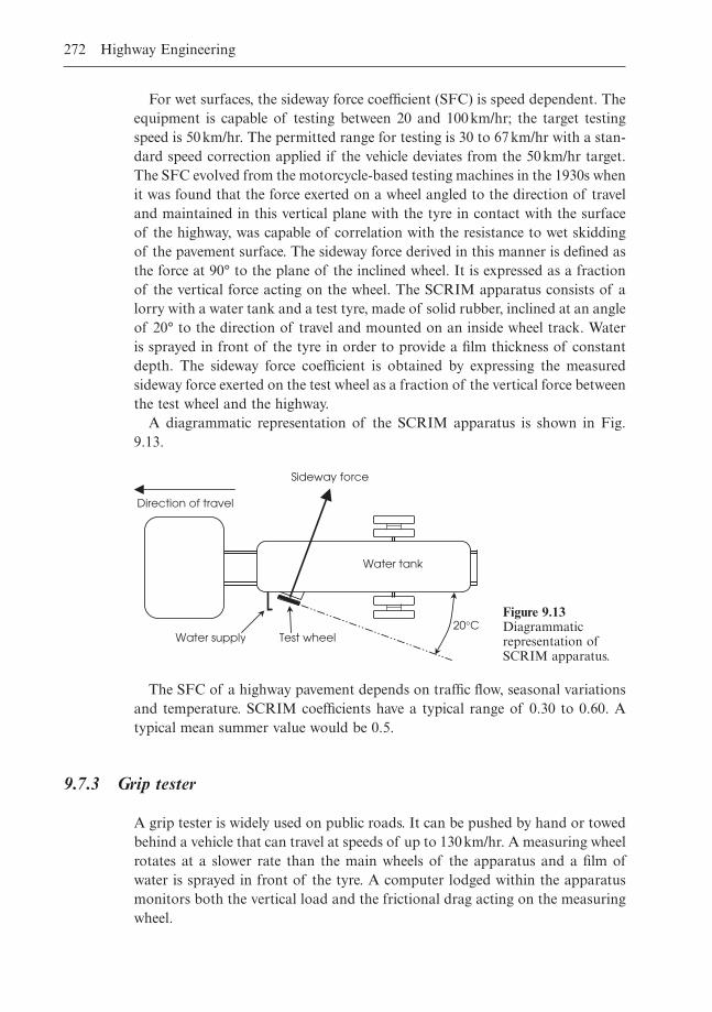
For wet surfaces, the sideway force coefficient (SFC) is speed dependent. Theequipment is capable of testing between 20 and 100km/hr; the target testingspeed is 50km/hr. The permitted range for testing is 30 to 67km/hr with a stan-dard speed correction applied if the vehicle deviates from the 50km/hr target.The SFC evolved from the motorcycle-based testing machines in the 1930s whenit was found that the force exerted on a wheel angled to the direction of traveland maintained in this vertical plane with the tyre in contact with the surfaceof the highway, was capable of correlation with the resistance to wet skiddingof the pavement surface. The sideway force derived in this manner is defined asthe force at 90° to the plane of the inclined wheel. It is expressed as a fractionof the vertical force acting on the wheel. The SCRIM apparatus consists of alorry with a water tank and a test tyre, made of solid rubber, inclined at an angleof 20° to the direction of travel and mounted on an inside wheel track. Wateris sprayed in front of the tyre in order to provide a film thickness of constantdepth. The sideway force coefficient is obtained by expressing the measuredsideway force exerted on the test wheel as a fraction of the vertical force betweenthe test wheel and the highway.
A diagrammatic representation of the SCRIM apparatus is shown in Fig.9.13.
272 Highway Engineering
Direction of travel
Water supply20∞C
Water tank
Test wheel
Sideway force
Figure 9.13Diagrammaticrepresentation ofSCRIM apparatus.
The SFC of a highway pavement depends on traffic flow, seasonal variationsand temperature. SCRIM coefficients have a typical range of 0.30 to 0.60. Atypical mean summer value would be 0.5.
9.7.3 Grip tester
A grip tester is widely used on public roads. It can be pushed by hand or towedbehind a vehicle that can travel at speeds of up to 130km/hr. A measuring wheelrotates at a slower rate than the main wheels of the apparatus and a film ofwater is sprayed in front of the tyre. A computer lodged within the apparatusmonitors both the vertical load and the frictional drag acting on the measuringwheel.
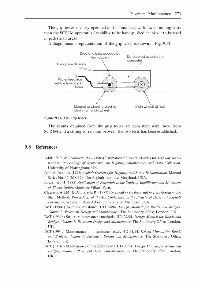
The grip tester is easily operated and maintained, with lower running coststhan the SCRIM apparatus. Its ability to be hand-pushed enables it to be usedin pedestrian areas.
A diagrammatic representation of the grip tester is shown in Fig. 9.14.
Pavement Maintenance 273
Measuring wheel rotated by chain from main wheel
Main wheels (2 No.)
Data stored by onboard computer
Drag and load gauged by transducers
Water feed fromvehicle towing grip
tester
Towing mechanism
Figure 9.14 The grip tester.
The results obtained from the grip tester are consistent with those fromSCRIM and a strong correlation between the two tests has been established.
9.8 References
Addis, R.R. & Robinson, R.G. (1983) Estimation of standard axles for highway main-tenance. Proceedings of Symposium on Highway Maintenance and Data Collection,University of Nottingham, UK.
Asphalt Institute (1983) Asphalt Overlays for Highway and Street Rehabilitation. ManualSeries No. 17 (MS-17). The Asphalt Institute, Maryland, USA.
Boussinesq, J. (1885) Application of Potentials to the Study of Equilibrium and Movementof Elastic Solids. Gauthier-Villars, Paris.
Claessen, A.I.M. & Ditmarsch, R. (1977) Pavement evaluation and overlay design – TheShell Method. Proceedings of the 4th Conference on the Structural Design of AsphaltPavements, Volume 1. Ann Arbor, University of Michigan, USA.
DoT (1994a) Skidding resistance, HD 28/94. Design Manual for Roads and Bridges,Volume 7: Pavement Design and Maintenance. The Stationery Office, London, UK.
DoT (1994b) Structural assessment methods, HD 29/94. Design Manual for Roads andBridges, Volume 7: Pavement Design and Maintenance. The Stationery Office, London,UK.
DoT (1994c) Maintenance of bituminous roads, HD 31/94. Design Manual for Roadsand Bridges, Volume 7: Pavement Design and Maintenance. The Stationery Office,London, UK.
DoT (1994d) Maintenance of concrete roads, HD 32/94. Design Manual for Roads andBridges, Volume 7: Pavement Design and Maintenance. The Stationery Office, London,UK.

DoT (1999) Maintenance assessment procedure, HD 30/99. Design Manual for Roadsand Bridges, Volume 7: Pavement Design and Maintenance. The Stationery Office,London, UK.
DoT (2001) Pavement design and construction, HD 26/01. Design Manual for Roads andBridges, Volume 7: Pavement Design and Maintenance. The Stationery Office, London,UK.
Kennedy, C.K., Fevre, P. & Clarke, C. (1978a) Pavement Deflection: Equipment for Mea-surement in the United Kingdom. TRRL Report LR 834. Transport and Road ResearchLaboratory, Crowthorne, UK.
Kennedy, C.K. & Lister, N.W. (1978b) Prediction of Pavement Performance and the Designof Overlays. TRRL Report LR 833. Transport and Road Research Laboratory,Crowthorne, UK.
Mayhew, H.C. & Harding, H.M. (1987) Thickness design of concrete roads. Departmentof the Environment, Department of Transport, TRRL Report RR 87. Transport andRoad Research Laboratory, Crowthorne, UK.
Roe, P.G. & Hartshorne, S.E. (1998) The polished stone value of aggregates and in-serviceskidding resistance. TRL Report 322, Transport Research Laboratory, Crowthorne,UK.
274 Highway Engineering

coated macadams, 214COBA, 56, 57, 66comfort criteria, 179community effects, 64concrete overlays, 264
design, 267concrete paving process, 224cone penetrometer, 198construction disturbance, 63construction joints, 221, 223construction of bituminous road surfacings, 218continuously reinforced concrete pavements, 248contraction joints, 221, 222crossfalls, 183cultural heritage, 63cumulative design traffic, 205curing, 227cutback bitumen, 211
damage factor, 231, 233deflectograph, 253, 255delay per arriving vehicle, 113delay per unit time, 113demand modelling, 16dense bitumen macadam (DBM), 214Department of Transportation, 1departures, 163design hourly volume (DHV), 90design life, 230, 231, 232, 233design reference flow (DRF), 103, 104, 127design speed, 155destinations, 23deterrence function, 23directional design hourly volume (DDHV), 91disutility, 16dowel bars, 224dry density, 195
ecology, 63economic appraisal, 45E-factors, 99, 100effective green time, 138
Index
actual green timemaximum, 149minimum, 148, 149
aggregates, 217air quality, 63alignment constraint, 158all-or-nothing, 35amber time, 141, 146annual average daily traffic (AADT), 68, 69, 104appraisal summary table, 71approach half-width, 126ARCADY, 105asphalts, 216average effective flare length, 126average queue lengths, 144average speed, 74average vehicle delays, 142
basecourse, 193bendiness, 158, 159benefit-cost ratio, 52, 56bitumen, 209bitumen-bound overlays, 264bituminous emulsions, 212brainstorming, 47
California bearing ratio (CBR), 194capacity at roundabouts, 125capacity of turning traffic streams, 110capping, 192, 200, 201
layer, 200carriageway widths, 153–5categories of pavement type, 193–4CBM1, CBM2, CBM3, CBM4, CBM5, 202cement-bound layers, 202–3central reservation, 153chippings, 212circulating flows, 128circulatory carriageway, 131classification for commercial vehicles, 203closing time, 166coated chippings, 220

effective red time, 144entry
angle, 125, 126, 127, 131capacity, 129deflection, 131radius, 126, 131width, 126, 131
environmental impact assessment (EIS), 10, 62environmental impact table (EIT), 64, 65, 66equivalent surface foundation modulus (ESFM), 264European Commission, 62expansion joints, 221, 222
falling weight deflectometer (FWD), 265Federal Highways Agency, 1flexible pavements, 193, 208, 209flow-density relationship, 76foundations, 192free-flow speed, 74–5frequency of accidents, 50functional effectiveness, 73funding, 2Furness method, 27–31
geology, 64ghost island junctions, 107gravity model, 23–6grip tester, 272–3growth factor model, 26–7
hardshoulders/hard strips, 154–5HD 26/01, 238–42heavy duty macadam (HDM), 214–15high speed road monitor, 253–5highway capacity, 78–9Highway Capacity Manual, 79highway pavement definition, 192highway planning process, 3–9Highways Agency, 1horizontal alignment, 167–77hot rolled asphalt (HRA), 216hourly volume, 80
impedance, 23inscribed circle diameter (ICD), 126, 131intangible factors, 45intergreen period, 140internal rate of return (IRR), 52
jam density, 74joint details, 221–3joint repairs, 252jointed concrete pavements, 242–8
K-values, 179
land use, 63models, 18–19
276 Index
planning, 6landscape effects, 63layout constraint, 157–8level of service (LOS), 79liquid limit (LL), 197–8lost time, 138, 139, 140LR833, 258–62LR1132, 231–7
M-factors, 99, 100macrotexture, 227main central island, 132mastic asphalt, 216maximum service flow, 81measures of worth, 45microtexture, 227modal split, 31–4modified binders, 211–12multinomial logit choice model, 31–2
National Environmental Policy Act (NEPA), 12, 62nature conservation, 63net present value (NPV), 45, 52new approach to appraisal (NATA), 66–71
opposed traffic streams, 135–6optimum cycle time, 139–40origin, 8OSCADY, 146overlay design
bituminous roads, 260–63concrete roads, 264–70
overlaying, 209, 232overtaking sight distance, 165–7overtaking time, 165, 166
parabolic formula (vertical alignment), 180–3passenger car equivalents, 83–4, 136patching, 251pavement
deflection, 258, 265deterioration, 208–9maintenance (need for), 251
payback analysis, 59–61peak-hour factor (PHF), 80phasing, 133, 134PICADY, 105plastic limit (PL), 198plasticity index (PI), 198porous macadam, 215priority intersections, 103, 105–19Private Finance Initiative (PFI), 3
queue length, 113, 144
rational planning process, 9reasoned choice, 44–5reinforcement, 223–4

relaxations, 162–3rigid pavements, 193, 209Rivers and Harbours Act, 11Road Note 29, 230–1roadbase, 193, 230roundabouts, 103, 119–32rural roads, 157–62
safety time, 166saturation flow, 133–8savings in time, 49–50SCOOT, 150SCRIM, 271–2seasonality index, 99service flow (SF), 80sharpness of flare, 126, 127shift, 174–5sight distances, 163–7signal linkage, 146–51signalised intersections, 103, 132–44simple junctions, 106single lane dualling, 107skid resistance, 227–8space mean speed, 74speed-density relationship, 74–5speed-flow relationship, 76–8standard axles, 233, 234statutory constraints, 157stopping sight distance, 163–5stratification, 16subbase definition, 192, 200subgrade strength, 234surface dressing, 211–13
T-chart, 48time-and-distance diagram, 150
Index 277
toll charges, 2Traffic Appraisal Manual (TAM), 105traffic
assignment, 34–6density, 73flow, 73loading, 203–6noise, 63
transitions, 173–7TRANSYT, 150travel distance, 24travel time, 24trip, 15
distribution, 22–31generation, 19–22
unopposed traffic streams, 135urban roads, 156–7utility, 15, 16, 31
vehicle operating costs, 49vehicle travellers, 64verges, 154vertical alignment, 178–91vertical crest curve, 183–8vertical sag curve, 189–91vibration, 63visibility, 179–80visual condition surveys, 253–4
warping joints, 221, 223water quality, 64wearing course, 193, 194wet skidding, 270–71wire brushing, 228