Research Institute for Advanced Computer ScienceNASA Ames Research Center

Highly Parallel Computation

Walter F. Tichy

August 19, 1990

t

RIACS Technical Report TR-90.35

NASA Cooperadve Agreement Number NCC2-387

c_

(NASA-CR-188_71) HIGHLY PARALLELCQMPUTATION (Research Inst. for _dvanced

Computer Science) 34 p CSCL 09B

G3/62

N92-I1698

Unclas

0043071

https://ntrs.nasa.gov/search.jsp?R=19920002480 2018-06-22T03:44:31+00:00Z

r-

Highly Parallel Computation

Peter J. Denning

Walter F. Tichy

Research Institute for Advanced Computer ScienceNASA Ames Research Center

RIACS Technical Report TR-90.35

August 19, 1990

Highly parallel computing architectures are the only means to achieve the computational ratesdemanded by advanced scientific problems. A decade of research has demonstrated the feasibility ofsuch machines and current research focuses on which architectures are best suited for particularclasses of problems. The architectures designated as MIMD and SIMD have produced the bestresults to date; neither shows a decisive advantage for most near-homogeneous scientific problems.For scientific problems with many dissimilar parts, more speculative architectures such as neuralnetworks or dataflow may be needed.

This is a preprint of an article to appear in Science magazine.

Work reported herein was supported in part by Cooperative Agreement NCC2-387between the National Aeronautics and Space Administration (NASA)

and the Universities Space Research Association (USRA).

Highly Parallel Computation

Peter J. Denning and Waiter F. Tichy

August 19, 1990

This paper has been accepted for publication

in Science magazine during fail 1990.

P. J. Denning is Research Fellow of theResearch Institute for Advanced Computer Science

NASA Ames Research Center

Moffett Field, CA 94035 USA

W. F. Tichy is in the Computer Science Department of theUniversity of Karlsruhe, FRG

ABSTRACT: Highly parallel computing architectures are the only means to

achieve the computational rates demanded by advanced scientific problems. Adecade of research has demonstrated the feasibility of such machines and current

research focuses on which architectures are best suited for particular classes of

problems. The architectures designated as M1MD and SIMD have produced the

best results to date; neither shows a decisive advantage for most near-homogeneous

scientific problems. For scientific problems with many dissimilar parts, more

speculative architectures such as neural networks or dataflow may be needed.

Work reported herein was supportedunderCooperative AgreementNCC2-38"/between the National Aeronautics_mdSpaceAdministration(NASA) andthe Universities SpaceResearch Association (USRA).

HPC

PRECEDING PAGE BLANK NOT FILMED

-3- TR-9035 (August 19, 1990)

Computation has emerged as an important new method in science. It gives access

to solutions of fundamental problems where pure analysis and pure experiment cannot

reach. Aerospace engineers, for example, estimate that a complete numerical simulation

of an aircraft in flight could be performed in a matter of hours on a supercomputer

capable of sustaining at least 1 trillion floating point operations per second (teraflops, or

tflops). Researchers in materials analysis, oil exploration, circuit design, visual

recognition, high energy physics, cosmology, earthquake prediction, atmospherics,

oceanography, and other disciplines report that breakthroughs are likely with machines

that can compute at a tflops rate.

The fastest workstations today operate at maximum speeds of slightly beyond 10

million flops (megafiops, or rnflops). In contrast, the fastest supercomputers have peak

rates in excess of 1 billion flops (gigaflops, or gflops) -- e.g., the NEC SX-2 is rated at 1.0

gflops and Cray Y-MP at 2.7 gflops. Even faster ones are coming: the 4-processor NEC

SX-3 (1990) will have peak rate of 22 gflops and the Cray 4 (1992) 128 gflops. When

recompiled for these machines, standard Fortran programs typically realize 10% to 20%

of the peak rate. When algorithms are carefully redesigned for the machine architecture,

they realize 70% to 90% of the peak rate [1]. There is an obvious payoff in learning

systematic ways to design algorithms for parallel machines.

Gordon Bell anticipates that machines capable of 1 tflops containing thousands (or

even millions) of processors will be available as early as 1995 [2]. For example, IBM

Research is developing the Vulcan machine, which will consist of 32,768 (215) 50-rnflops

processors, and Thinking Machines Corporation is considering a Connection Machine

with over a million (22°) processors. These supermachines may cost on the order of $50

HPC -4- TR.g0 35 (August 19,1990)

millions apiece. Bell anticipates that low-cost, single-processor, reduced instruction set

chips (RISC) with speeds on the order of 20 mflops will be common in workstations by

1995. It is clear that tflops machines will be multicomputers consisting of large numbers

of processing elements (processor plus memory) connected by a high-speed message

exchange network. Smaller multicomputers will proliferate in the next five years: we

must learn to program them.

Speedup is a common measure of the performance gain from a parallel processor. It

is defined as the ratio of the time required to complete the job with one processor to the

time required to complete the job with N processors [3]. Perfect speedup, a factor of N,

can be attained in one of two ways. In a machine were each piece of the work is

permanently assigned to its own processor, it is attained only when the pieces are

computationally equal and processors experience no significant delays in exchanging

information. In a machine where work can be dynamically assigned to available

processors, it is attained as long as the number of pieces of work ready for processing is

at least N.

In discussing speedup, it is important to distinguish between problem size and

computational work. Problem size measures the number of elements in the data space

and computational work the number of operations required to complete the solution. For

example, an NxN square matrix occupies N 2 storage locations and it takes about N 3

operations to form the product of two of them. Doubling the dimension multiplies the

storage requirement by four and the computational work by eight. Conversely, doubling

the number of processors would permit multiplying two matrices of dimension 26%

larger in the same amount of time. This has important consequences for multiprocessors:

HPC -5- TR.9035 (August 19, 1990)

there may be too few processors available to achieve speedup that is linear in problem

size. The best we can achieve is speedup that is linear in the number of processors.

A study in 1988 at Sandia National Laboratory provided the first case of near-

perfect speedup for three problems involving the solutions of differential equations on a

machine with 1024 processors [4]. Later that year, Geoffrey Fox published a study of 84

parallel algorithms reported in the scientific literature and concluded that 90% of them

could be extrapolated to larger machines with speedups proportional to the number of

processors [5]. These results give considerable grounds for optimism about speedup on

other problems.

The central question of the early 1980s was whether parallel computation would

become practical. This question has been settled and we have moved on to bigger

questions. What are the best parallel architectures for given classes of problems? How

can we partition a given problem into thousands of parts that can be independently

executed on different processors? How do we design algorithms so that delays of

interprocessor communication can be kept to a small fraction of the computation time?

How can we design the parts so that the load can be distributed evenly over the available

processors? How can we design the algorithms so that the number of processors is a

parameter and the algorithm can be configured dynamically for the available machine?

How can we prove that a parallel algorithm on a given machine meets its specifications?

How do we debug programs, especially when the results of flawed parallel algorithms

may not be precisely reproducible?

HPC -6. TR.9035 (August19,1990)

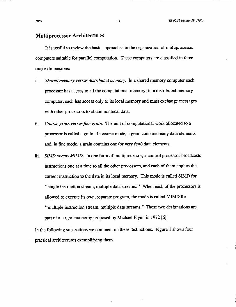
Multiprocessor Architectures

It is useful to review the basic approaches in the organization of multiprocessor

computers suitable for parallel computation. These computers are classified in three

major dimensions:

i. Shared memory versus distributed memory. In a shared memory computer each

processor has access to all the computational memory; in a distributed memory

computer, each has access only to its local memory and must exchange messages

with other processors to obtain nonlocal data.

ii. Coarse grain versus.fine grain. The unit of computational work allocated to a

processor is called a grain. In coarse mode, a grain contains many data elements

and, in fine mode, a grain contains one (or very few) data elements.

iii. SIMD versus MIMD. In one form of multiprocessor, a control processor broadcasts

instructions one at a time to all the other processors, and each of them applies the

current instruction to the data in its local memory. This mode is called SIMD for

"single instruction stream, multiple data streams." When each of the processors is

allowed to execute its own, separate program, the mode is called MIMD for

"multiple instruction stream, multiple data streams." These two designations are

part of a larger taxonomy proposed by Michael Flynn in 1972 [6].

In the following subsections we comment on these distinctions. Figure 1 shows four

practical architectures exemplifying them.

HPC -7- TR.9035 (August 19, 1990)

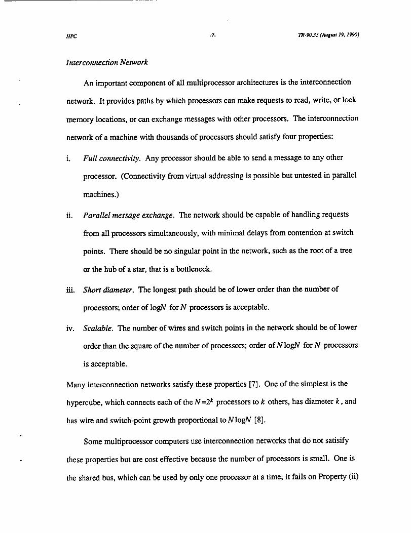
lnterconnection Network

An important component of all multiprocessor architectures is the interconnection

network. It provides paths by which processors can make requests to read, write, or lock

memory locations, or can exchange messages with other processors. The interconnection

network of a machine with thousands of processors should satisfy four properties:

i. Full connectivity. Any processor should be able to send a message to any other

processor. (Connectivity from virtual addressing is possible but untested in parallel

machines.)

ii. Parallel message exchange. The network should be capable of handling requests

from all processors simultaneously, with minimal delays from contention at switch

points. There should be no singular point in the network, such as the root of a tree

or the hub of a star, that is a bottleneck.

iii. Short diameter. The longest path should be of lower order than the number of

processors; order of logN for N processors is acceptable.

iv. Scalable. The number of wires and switch points in the network should be of lower

order than the square of the number of processors; order of N logN for N processors

is acceptable.

Many interconnection networks satisfy these properties [7]. One of the simplest is the

hypercube, which connects each of the N=2 k processors to k others, has diameter k, and

has wire and switch-point growth proportional to NlogN [8].

Some multiprocessor computers use interconnection networks that do not satisify

these properties but are cost effective because the number of processors is small. One is

the shared bus, which can be used by only one processor at a time; it falls on Property (ii)

HPC -8- TR-9035 (August 19, 1990)

because when the number of processors approaches 100 in current designs, bus

contention becomes so severe that the bus saturates and limits the speed of the machine.

Examples of computers that use it are Sequent Symmetry and Encore Multimax.

Another is the crossbar switch, which provides every processor with a path to every

memory; it fails on Property (iv) because it contains N 2 switch points and becomes

unwieldy for more than a few hundred processors. Examples of computers that use it are

Cray X-MP and Cray Y-MP, where the crossbar switching logic is distributed among the

individual memory units.

Shared v. Distributed Memory

The shared memory architecture was introduced by Burroughs in the B5000

machine in the late 1950s and is used today in machines like the Sequent Balance and

Encore Multimax. It gives all processors equal access to all memories through the

interconnection network. Messages of any length can be exchanged in the fixed time

required to exchange the address of the message header. The distributed memory

architecture gives each processor direct access to only one memory unit, the local

memory; access to other data is gained by sending messages through the interconnection

network. Message exchange time is proportional to message length. This approach is

economical if local accesses are more frequent than other accesses.

The strategy of designing algorithms for full sharing of all memory by all

processors has an important fundamental limitation. Because individual memory

modules can be accessed by only one processor at a time, all but one of the processors

seeking access to a given module will be blocked for the duration of that module's cycle

HPC -9- TR-9035 (August 19, 1990)

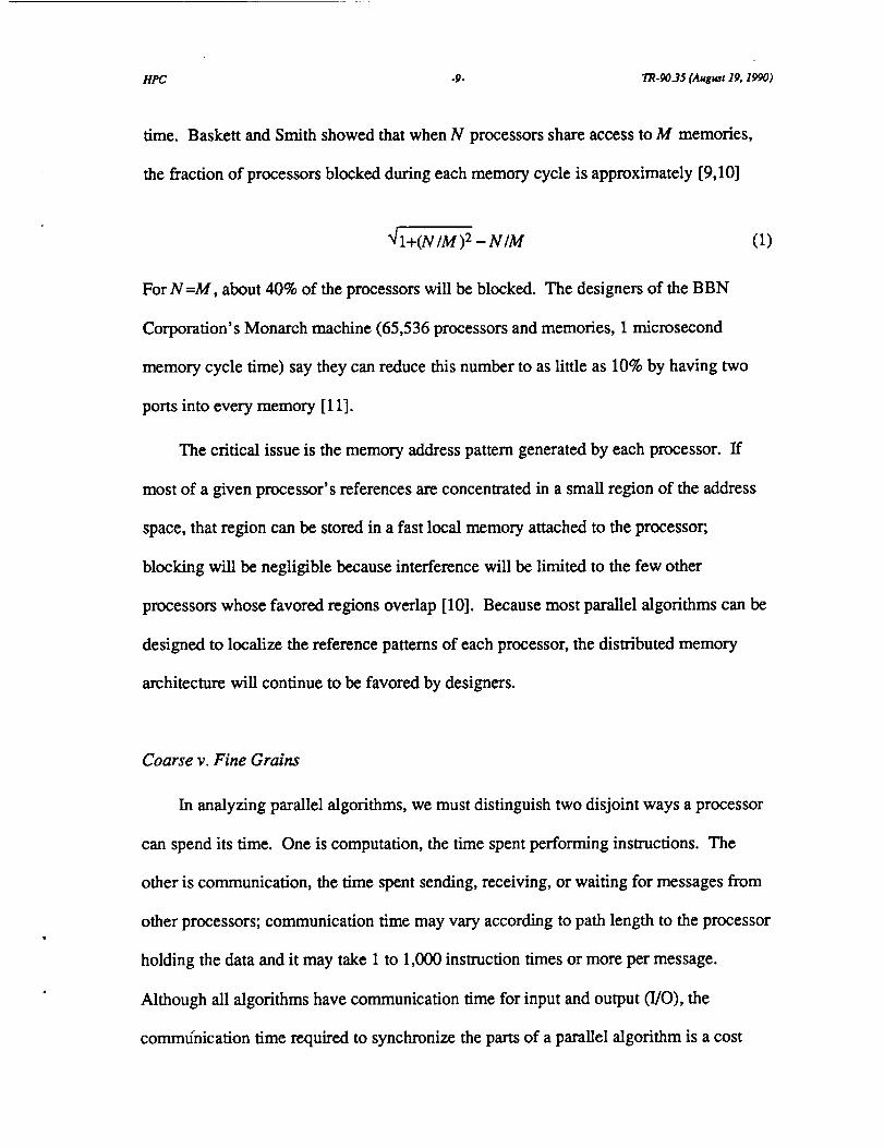
time. Baskett and Smith showed that when N processors share access to M memories,

the fraction of processors blocked during each memory cycle is approximately [9,10]

I+(N/M)2 _ N/M (1)

For N =M, about 40% of the processors will be blocked. The designers of the BBN

Corporation's Monarch machine (65,536 processors and memories, 1 microsecond

memory cycle time) say they can reduce this number to as little as 10% by having two

ports into every memory [11].

The critical issue is the memory address pattern generated by each processor, ff

most of a given processor's references are concentrated in a small region of the address

space, that region can be stored in a fast local memory attached to the processor;

blocking will be negligible because interference will be limited to the few other

processors whose favored regions overlap [10]. Because most parallel algorithms can be

designed to localize the reference patterns of each processor, the distributed memory

architecture will continue to be favored by designers.

Coarse v. Fine Grains

In analyzing parallel algorithms, we must distinguish two disjoint ways a processor

can spend its time. One is computation, the time spent performing instructions. The

other is communication, the time spent sending, receiving, or waiting for messages from

other processors; communication time may vary according to path length to the processor

holding the data and it may take 1 to 1,000 instruction times or more per message.

Although all algorithms have communication time for input and output (I/O), the

commtlnication time required to synchronize the parts of a parallel algorithm is a cost

HPC -I0. TR-9035 (Au&wt Jg,1990)

that is not present in sequential algorithms.

The computational utilization Ui of a processor i is the fraction of time that

processor is executing computational instructions; thus 1-Ui is the fraction of time that

processor is executing communication instructions or waiting for messages. The speedup

attained by a computation with N processors is at most U I+U2+...+Ut¢; it may be less if

portions of the computation are repeated in several grains. The maximum speedup of N

will be achieved by an algorithm in which the computational utilization of each processor

is near 1 and there is little redundant computation.

In many algorithms for physical problems, each processor is assigned a region of

space containing a cluster of points on the grid over which the differential equations are

solved. In a two-dimensional grid, a square with k points on an edge will have

computational work proportional to the number of points, k 2, and communication

proportional to the perimeter, 4k. With k sufficiently large, the computational work will

be large compared to the communication, which means each Ui will be close to 1 and N

such processors will produce nearly perfect speedup.

Now we see why grain size is important. The architecture will determine the cost of

a communication step relative to a computation step. If the cost is high, the algorithm

designer will favor large grains containing many instructions for each message; the

number of subprograms will be a small function of the problem size. If the cost is low,

the algorithm designer can afford small grains and the number of grains will be

proportional to problem size. In specifying algorithms that will scale for larger

machines, designers tend to choose grain sizes at the point of diminishing returns

between computation and communication; for this reason, when given a machine with

HPC -11- TR-9035 (Aught 19, 1990)

more processors, they use it for a larger problem at the same grain size rather than for the

same problem with a smaller grain size [4].

The attraction of fine grains is that they afford the largest possible amount of

speedup. They are practical in certain limited cases today, most often signal and image

processing problems and problems involving particle tracing. Machines illustrating this

are the Connection Machine [12] and the Goodyear/NASA Massively Parallel Processor

(MPP) [13]. In these cases, the machines are able to move a data element between

immediately neighboring processors in time comparable to the instruction time, and

many computations over grids of such elements will achieve individual processor

computational utilizations of 0.5 or greater at the finest grain.

SIMD v. MIMD

A fundamental question in the design of parallel algorithms is how to guarantee

that, when a processor executes an instruction, the operands of that instruction have

already been computed by previous instructions. Without this guarantee, the results of

the comptuation can be indeterminate and depend on the relative speeds of the processors

(race conditions). The mechanism that provides this guarantee is called synchronization.

Synchronization is straightforward in standard sequential single-processor

machines, where instructions are executed one at a time. The results of each instruction

are left in registers or in memory for access by later instructions. Optimizing compilers

for such machines may exchange the order of instructions that do not provide data to

each other. A direct extension of this mode for multiprocessing appears on machines of

the SIMD type, where each instruction is simultaneously obeyed by all the processors.

HPC -12. TR-9035 (August 19, 1990)

An example will illustrate. Suppose that a difference equation on a grid calls for

averaging the values at the four nearest neighbors of a point; the programming language

expression for the operation to be applied at point (i ,j) would read

v(i,j) = [ v(i-l,j)+v(i+l,j)+v(i,j-1)+v(i,j+l)) /4 (2)

On the SIMD machine, we can associate one data processor with each point on the grid;

its memory holds the value v (i,j). The control processor broadcasts the instructions

implementing Expression (1) to all the data processors, which obey them using their own

particular values of i and j. Programs of this kind are easy to understand because they

look almost the same as their counterparts for a single-processor machine. HiUis and

Steele, in fact, say that the best way to think of SIMD programming is sequential

programming in which each operation applies simultaneously to sets of data rather than

to individual data elements [14]. It is impossible to program races in SIMD algorithms.

Under the MIMD mode, each processor has its own separate program of instructions

to obey. The programs need not be identical. Now the machine must provide explicit

means for synchronization. The hardware must supply buffers for passing messages

between processors, flags to indicate the arrivals of signals and messages, and

instructions that stop and walt for the flags. The programmer must use these

synchronization instructions where a definite order of events must be established. For

example, Expression (2) becomes

PUT (v ,i-l,j )

PUT (v ,i+l,j)

PUT (v,i j-1)

PUT(v ,i d+l)

v = (GET (i - 1,j)+GET (i + 1,j )+GET (i ,j - I)+GET (i ,j + 1))/4

HPC -13. TR.9035 (Ausust 19,1990)

where PUT sends a message containing the value of v to a designated processor and

GET waits until a message is received from a designated processor; a GET must match

the corresponding PUT on the sending processor. Obviously this increases the

programming effort and exposes the programmer to errors that arise when these new

operations are used improperly. (Think what would happen if the four PUT statements

did not all precede the GETs.)

The main limitation of the SIMD architecture is its restriction that all processors

must execute the same instruction. Even in highly regular problems there are

differences, such as the evaluation of boundary conditions, that require different

algorithms for some processors than others. The machine must shut off boundary

processors while broadcasting the instructions for interior nodes, and it must shut off

interior processors while broadcasting instructions for boundary nodes. The need to shut

off some of the processors lowers the utilization of the machine and the speedup it can

attain. An MIMD architecture, which can execute the interior and boundary algorithms

in parallel, does not suffer from this limitation.

Practical Considerations

There are at least eight distinguishable architectures corresponding to the various

combinations of the factors above. In practice to date in scientific computing only three

of these possibilities have been used:

MIMD coarse shared

MIMD coarse distributed

SIMD fine distributed

Sequent, Encore, Alliant, Convex, Cray

hypercubes (Intel, Ametek, NCube)

Connection Machine, MPP

HPC -14- TR-90.35(AugustJ9,1990)

There are two reasons for this. First, the shared memory architecture has been of limited

use in large computations because fewer than a hundred processors are enough to saturate

the common bus; such architectures do not extend to thousands of processors. Moreover,

there are no reported test cases in which shared memory was a distinct advantage even

when a small number of processors was sufficient [5]. Second, the grain size is normally

the consequence of the communication structure of the machine and the nonlocal

referencing patterns of the algorithm. MIMD machines to date have used coarse grains

because synchronization costs would be too high with fine grains. Only the S1MD

architecture has been successful with fine grains, and then only with each processor

having its own local memory.

The predominence of these three architecture types today does not mean that others

are forever impractical. We will discuss later the dataflow architecture, which is capable

of supporting fine grain parallelism within the MIMD mode and may become practical

by the end of the decade.

As discussed by Hopfield and Tank, neural networks can be used for special

purpose combinatorial optimization and pattern recognition problems [15]. They

represent another architectural type that can be used for highly parallel computation.

They are not of direct interest in the numerical computations that predominate in

computational science, but they may be of indirect interest for ancillary combinatorial

issues such as automatic grid generation and mapping grids to the nodes of a hypercube.

HPC -15- TR-9035 (Ausust 19, 1990)

Problem Classes

Let us turn now to the types of problems that have proved to be most amenable to

efficient execution on highly parallel computers. The good news is that for a wide range

of scientific problems, at least one of the three architectural types noted above works well

[5].

Fox has proposed a classification of problems into three broad categories [5].

Synchronous problems are ones in which the physical equations specify the behavior at

every point in the data space for every small increment of time. Loosely synchronous

problems are ones for which there are embedded time sequences (renewal points) at

which the physical equations specify the values of the data elements; in between these

times there is no global specification of the data values in local regions of data space.

Asynchronous problems are all the rest. Fox says that most of the results in the literature

have been obtained for the first two types classes of problems and that we have not yet

learned how to divide problems into dissimilar pieces that can keep an MIMD machine

busy.

Single-Function Problems

We now reformulate these notions of problem classes in a way that more clearly

reveals which types of problems are best suited for types of architectures.

Many computational problems have the characteristic that a simple procedure must

be applied uniformly across a large number of data elements organized within a data

structure. We can specify the procedure by a sequential algorithm in which each step is

an operation applied simultaneously to all the data elements. The design of such "data

HPC -16- TR.9035 (August 19. 1990)

parallel" algorithms closely resembles ordinary programming in languages such as

Fortran or C.

Physical problems modeled by a set of differential equations are common

paradigms for data parallel algorithms. The continuum equations are modeled by a set of

difference relations among dependent quantitites associated with points on a discrete

grid. The difference relations are usually the same for all points except the boundaries.

In a data parallel algorithm each grid point is assigned its own processor that contains a

program to evaluate the difference relation. Because the difference relation depends only

on the immediately adjacent grid points, each processor need communicate only with a

small number of others in its neighborhood.

The class of problems amenable to data parallel solution is by no means limited to

differential equation models. Others include:

i. Searching. Find data elements satisfying a given property. If processors are as

numerous as data elements, the search can be completed in a constant amount of

time independent of the data set and the result reported in an additional logN time.

ii. Sorting. Arrange a sequence of data elements in order. If processors are as

numerous as data elements, the sort can be completed in time proportional to log2N

on N processors.

iii. Joining tables in a database. Form a new table from two others having a common

column, by combining a record from one table with a record in the other whenever

they have the same value in the common column. This can be done in time

proportional to the size of the larger table if processors are numerous.

HPC -17- TR._0 35 (Ausust 19, 1990)

iv. Computational Geometry. Find the convex hull of a set of points. With N

processors and N points, this can be done in average time proportional to log2N.

v. Solving Linear Equations. Find the solution of a set of equations of the matrix form

Ax =b. With N processors and N unknowns, the parallel Gauss-Jordan method

obtains the solution in time proportional to N2; with N 2 processors, the time drops

to N logN.

vi. Fast Fourier Transform. Find the one-dimensional Fourier transform of a series of

points. With N processors and N points, this can be done in time proportional to

logN.

This list is merely suggestive: it indicates that a large variety of subproblems that

commonly arise in computational libraries are data parallel and subject to considerable

speedup on machines containing large numbers of processors [16,17].

Practical data parallel algorithms must be designed to adapt to the number of

processors actuafly available. For example, 1,000,000 data elements can be searched by

1,000 processors in time proportional to logl000 by performing a binary search on the

1,000 elements allocated to each processor. Optimal combinations of sequential and

parallel components are open problems in parallel algorithm design.

It is important to remember that data parallel algorithms cannot be universally

guaranteed to keep all the processors busy all the time. An illustration is an image

processing algorithm that operates in two passes. On the first, the algorithm determines

local features of chunks of the image and, on the second, it locates contours by joining

the local features across chunks. Processors assigned to chunks having few features will

also have little work to do. Because the proportion of processors that can be kept busy is

HPC -18- TR.9035 (Au&ust 19, 1990)

dependent on the input data, one cannot expect that the speedup will be proportional to

the number of processors.

Multiple-Function Problems

Many computational problems involve many functions composed together.

Examples include finite element analysis over nonhomogeneous rigid structures, multi-

zone fluid flow calculations, circuit simulations, fluid flows in nonhomogeneous

subterranean formations, and multidisciplinary models. These problems cannot be

regarded as data parallel; they must instead be regarded as a network of machines

performing different functions and exchanging data. They correspond to Fox's

asynchronous problems. Their algorithms are today commonly written in C or Fortran.

Many researchers believe that process-oriented languages such as Occam [18] and

functional composition languages such as VAL [19] or FP [20] would produce more

concise descriptions of algorithms for these problems.

Architectural Matching

From these descriptions it is obvious that single-function (data parallel) problems

are well suited to the SIMD architecture, and multi-function problems are well suitedto

the MIMD architecture. A major impediment to solving multi-function problems to date

has been the lack of programming languages that express functional composition easily.

The main barrier to the widespread use of such languages is cultural. The scientific

community has used Fortran for so many years that programming with new languages is

unfamiliar and will remain untried as long as the scientific investigator sees no value to

HPC -19- TR-9035 (Auguat 19, 1990)

learning it. The ability to express solutions to multi-function problems may be a

sufficient motivation to learn this later in the 1990s.

Connection Machine

To make concrete the previous points about solving single function problems on an

SIMD machine, we will consider the architecture and programming of a particular SIMD

machine, the Connection Machine 2 manufactured by Thinking Machines Corporation.

The Connection Machine model 2 (CM2) is an SIMD computer with 65,536 (216)

processors connected in a 16-dimensional hypercube network. Each processor has 32

kilobytes of local memory; the entire primary memory of a CM2 is 2 gigabytes (231

bytes). The processors collectively have the capacity to be a supercomputer that solves

very large problems with data parallel methods.

The CM2 cycles between intervals of instruction execution and message exchange.

At the start of an instruction interval, the control processor broadcasts an instruction to

all processors; the subset of them that are enabled execute that instruction using data in

their local memories. During a message exchange interval, processors copy values

required during the next instruction interval. It is easy for compilers to determine the

source and destination addresses of these messages. If an algorithm uses many long

paths in the network, the message interval can be 50-250 floating-point instruction times,

severely limiting the computational rate of the machine.

The CM2 configures algorithms for the number of processors actually present

through the method of virtual, or simulated, processors. The programmer designs an

HPC -20- TR-#0 35 (Augwst 19, 1990)

algorithm just once, assuming that the machine has the required number of processors.

The compiler assigns sets of the programmer's virtual processors to each available

processor on the CM2, and that processor simulates the execution of all the virtual

processors assigned to it. The maximum number of virtual processors is limited by the

available memory. As an example, we can assign a virtual processor to every point in a

1024 by 1024 image (220 points); each of the CM2's 216 processors must simulate 16

virtual processors, each limited to 1/16th of the memory and 1/16 the speed of a

processor.

Programmers use standard languages (Lisp, Fortran, C) on the CM2. We will

review how standard control statements operate on the CM2. Consider a selection

statementof the form IF C THEN A ELSE B:

i. The control processor broadcasts the instructions that evaluate the test C; at the end

of this sequence, each processor contains the value TRUE or FALSE. The control

processor broadcasts an instruction telling all processors containing FALSE to turn

themselves off.

ii. The control processor broadcasts the instructions for the clause A; those instructions

will be obeyed by the subset of processors still on. At the completion of this

sequence, the control processor broadcasts an instruction telling all processors to

reverse their status between on and off.

iii. The control processor broadcasts the instructions for the clause B; those instructions

will be obeyed by the subset of processors now on. At the completion of this

sequence, the control processor broadcasts an instruction telling all processors to

turn themselves on.

HPC -21- TR-90.35 (Au&_t 19, 1990)

The CM2 implements the on and off status of processors with a one-bit register per

processor called the context flag. When the context flag is FALSE, the associated data

processor is off; when off, it obeys only instructions that unconditionally manipulate

context flags.

An iteration statement such as WHILE C DO A works similarly. The control

processor broadcasts the instructions of the test C and then the command for all

processors containing FALSE to turn themselves off. It then broadcasts the instructions

of A and only the processors still on execute it. This is repeated until all processors have

shut themselves off. Thereafter the control processor instructs them all to turn

themselves on again.

Because the programming syntax for the CM2 is basically unchanged from familiar

sequential machines, many algorithms can easily be converted for the CM2.

Unfortunately many sequential algorithms converted in such a straightforward,

mechanical way are not efficient for a parallel machine. Figure 2 illustrates the point for

matrix multiplication [21]. For this reason, much of the research to date in algorithms for

parallel machines has been a complete rethinking that has produced some unexpectedly

new designs that do not resemble their counterparts for sequential computers

[16,17,21,22].

HPC -22- TR.9035 (August 19, 1990)

Dataflow Computers

Dataflow computers are the most practical form of MIMD fine-grained parallel

computers known. They limit the cost of synchronization and afford a high degree of

parallelism by replacing control flow with data flow. Under control flow, each processor

has an instruction pointers that designates which instructions are enabled for execution.

Under dataflow, instructions become enabled for execution by the arrival of required

operands.

A dataflow program consists of a set of instruction packets stored in the memory of

the dataflow computer. An instruction packet is disabled until all its required operands

have arrived. Enabled instruction packets are sent via a distribution network to an array

of processors, where they are executed and their results distributed back to instruction

packets that await them. If a large number of instruction packets are enabled, a dataflow

computer with a large number of processors achieves high parallelism and high

utilization. A dataflow computer can offer fine grain parallelism because it can exploit

parallelism at the level of individual functions, expressions, and subexpressions [23].

Program statements that operate on arrays of data will achieve high speedups on a

dataflow machine. Consider again the earlier example of a computation over a grid of

points v (i ,j). In a dataflow computer, all the assignment instructions for all the grid

points would be enabled in parallel; each would await four operands generated by its four

neighbors, and would then produce a new result. The speed of the machine would be

directly proportional to N/M for N grid points and M processors. These findings were

confirmed by a study we performed jointly with NASA and DARPA in 1984 [24].

Benchmark studies on a prototype dataflow computer at the University of Manchester

HPC -23- TR.9035 (August 19, 1990)

have indicated that many sequential programs can also keep all the processors of a

dataflow computer busy [25].

A dataflow computer automatically solves the problem of assigning virtual

processors (here, instruction packets) to the real processors of the machine: as soon as a

virtual processor is enabled by the arrival of needed operands, it is sent to a real

processor for execution. Although the ratio of computation to communication time per

virtual processor may be low (0.01 to 0.1), utilization of the machine can nevertheless by

close to 1 if the program has sufficiently many instructions enabled at the same time.

Aside from a few university and commercial prototypes, no serious commercial

dataflow machine is available. There are several reasons for this. The SIMD machine is

simpler to build and can be programmed within familiar language concepts; the dataflow

machine requires new languages and new compiling technologies based on unfamiliar

concepts [19]. The SIMD machine uses a hypercube interconnection network, which is

cheap to build; the dataflow machine depends on a high-speed packet switched network,

a technology that is only now becoming inexpensive.

Some researchers are studying dataflow languages as source languages for SIMD

architectures. Experience with these languages will benefit the programming of all

parallel machines.

HPC -24- TR.9035 (August 19, 1990)

Conclusions

The sequential computer has been the dominant paradigm since the first ENIAC was

brought on-line in 1946. We are fast approaching the physical limits of this technology

while our computational needs continue to grow. After two decades of experimentation,

successful computers containing thousands of processors operating in parallel have been

built and are for sale in the market, and early experience with these machines in practice

has been highly encouraging. Many challenges lie ahead in computer architecture,

algorithms, programming languages, compilers, operating systems, performance

evaluation, software engineering, and the vast number of applications.

The new breed of massively parallel machines will in the long run have an impact

as profound as microcomputers. These machines are forcing us to rethink our

approaches to algorithms: any technology that brings about a change in the manner of

organizing work will have far-reaching effects.

HPC -25- TR.9035 (A_ust 19, 1990)

References and Notes

1. J.J. Dongarra, "Performance of various computers using standard linear equations

software in a Fortran environment," Computer Architecture News, 16, 47 (1988).

2. G. Bell, "The future of high performance computers in science and engineering,"

Comm. ACM, 32, 1091 (September 1989).

3. A.H. Karp and H. P. Flatt, "Measuring Parallel Processor Performance," Comm.

ACM, 33, 539 (May 1990).

4. J. Gustafson, G. Montry, and R. Benner, 'Development of parallel methods for a

102¢-processor hypercube," SIAMJ. Sci. Stat. Comp., 9, 1 (1988).

5. G.C. Fox, "What Have We Learnt from Using Real Parallel Machines to Solve

Real Problems?" Hypercube Concurrent Computers and Applications (ACM Press,

New York, 1988), pp. 897-955.

6. M.J. Flyrm, "Some computer organizations and their effectiveness," IEEE Trans.

on Comp. C-21,948 (September 1972).

7. H.J. Siegel, Interconnection Networks for Large-Scale Parallel Processing: Theory

and Case Studies (Lexington Books, 1985).

8. P.J. Denning, "Multigrids and hypercubes," American Scientist, 75, 234 (May

1987).

9. F. Baskett and A. J. Smith, "Interference in Multiprocessor Computer Systems with

Interleaved Memory," Comm. of ACM, 19 (June 1976).

10. P.J. Denning, "Is Random Access Memory Random?" American Scientist, 74, 126

(March-April 1986).

HPC -26- TR-9035 (Au&ust 19, 1990)

11. R.D. Rettberg, W. R. Crowther, P. P. Carey, and R. S. Tomlinson, "The Monarch

Parallel Processor Hardware Design," IEEE Computer, 23, 18-30 (April 1990).

12. D. Hillis, The Connection Machine (MIT Press, Cambridge, MA, 1985).

13. J.R. Fischer, Ed., Frontiers of massively parallel scientific computation.

Proceedings of symposium at NASA Goddard Space Flight Center, 24-25

September 1986, NASA Conference Publication 2478.

14. D. Hillis and G. Steele, "Data Parallel Algorithms," Comm. ACM, 12, 1170

(December 1986).

15. J.J. Hopfield and D. W. Tank, "Computing with Neural Circuits, a Model,"

Science, 233, 625 (1986).

16. S.G. Akl, The Design and Analysis of Parallel Algorithms (Prentice-Hall,

Englewood Cliffs, New Jersey, 1989).

17. A. Gibbons and W. Rytter, Efficient Parallel Algorithms (Cambridge University

Press, 1988).

18. Inmos, Ltd., Occam Programming Manual (Prentice-Hall, Englewood Cliffs, NJ,

1984).

19. J.R. McGraw, "The VAL Language: Description and Analysis," ACM Trans. on

Programming Languages and Systems, 4, 44 (January 1982).

20. J. Backus, "Can Programming be Liberated from the von Neumann Style?" Comm.

ACM, 21,613-641 (August 1978).

21. W.F. Tichy, "Parallel Matrix Multiplication on the Connection Machine," lnt'l J.

High Speed Computing, 2 (January 1989).

HPC -27- TR.9035 (August 19, 1990)

22. H.D. Simon, Ed., Scientific Applications of the Connection Machine (World

Scientific Publishing Co., 1989).

23. K. Hwang and F. A. Briggs, Computer Architecture and Parallel Processing

(McGraw-Hill, New York, 1984), pp. 748-768.

24. G.B. Adams III, R. L. Brown, P. J. Denning. "An Evaluation Study of Dataflow

Computation." Technical Report TR-85.2 (Research Institute for Advanced

Computer Science, NASA Ames Research Center, 230-5, Moffett Field, CA 94025,

1985) In this study, seven NASA teams programmed the MIT static dataflow

machine with kernel problems from their scientific domains. The machine was still

in design and not implemented. Five of the seven teams concluded they could keep

all 256 processors busy and achieve the full 1.28 gflops offered by the design. The

two others concluded that a scaled-down version of the machine (16 processors)

would be adequate. Weak aspects of the design were uncovered and slated for

improvement.

25. J.R. Gurd, C. C. Kirkham, and I. Watson, "The Manchester prototype dataflow

machine," Comm. ACM, 28, 34 (January 1985).

HPC .28- TR-9035 (August19,1990)

Figure Captions

FIGURE 1. The figures shows four computer architectures for parallel computation. The

first three are in common use and the fourth may become common by the end of the

decade. Organization (a) is an SIMD machine in which a single control processor

broadcasts a stream of instructions to all data processors. Each instruction calls for an

operation on data in local memory or for an exchange of data over the interconnection

network. Organization (b) is an MIMD machine in which processors running distinct

programs carry out operations on data in a set of memories shared by them all. All

processor-memory traffic passes through a high-speed interconnection network.

Organization (c) is an MIMD machine in which processors use local memory for most

operations and occasionally exchange data over an interconnection network.

Organization (d) is an MIMD dfataflow machine in which instruction packets in memory

flow to the processors for execution when all their operands are present; processors send

results back, where their arrivals trigger new instructions for execution.

FIGURE 2. Experiments on a Connection Machine reveal big differences in

performance and illustrate tradeoffs between storage requirements and running times on

parallel machines. The graph shows running time for three algorithms for multiplying

NxN matrices on a CM2 with 215 processors. Each curve is labeled with its asymptotic

growth rate in N. The upper curve is for the standard sequential algorithm that takes

time proportional to N 3 using one processor. The middle curve is an algorithm that uses

N 3 processors and takes time proportional to logN. The lower curve is an algorithm that

computes each of the N 2 results on a separate processor;, it takes time proportional to N.

HPC -29- TR-9035 (Au&ust 19, 1990)

The discontinuities in the two lower curves result from the simulation of virtual

processors. For each value of N=32, 40, 50, 64, 80, 100, 128 .... in the middle curve the

next stage of virtual processor simulation starts, with respectively 2, 4, 8, 16, 32, 64, 128,

... virtual processors per real processor; at each step the running time doubles and at

N=256 the machine runs completely out of memory. When N >181 in the lower

algorithm, N 2 > 215, and the running time doubles for the same reason.

controller

P

M

,r

P

M

J_

Instruction stream

V

P

M

v 11_

interconnection network

_r

P

M

J_

_r

(a) SlMD distributed

interconnection network

(b) MIMD shared

l

PI P Ii

' P I

MI M I MI

TT TI interconnection network

(c) MIMD distributed

_V

_T

4

V

P

r

• p

_V

results "_-IP"

enabled instructions

M M M

41,

(d) MIMD dataflow

RU

n

T

i

m

e

s

e

c

26 -

24 -

22 -

20 --

18 -

12 -

10 -

_

_

_

_

0

0

N 3

i

tiii

i

iiiiii

ii

/ N

I I I I I I I I I I

50 100 150 200 250

Matrix Dimension (N)