Higher genus Abelian functions associated with algebraic - ROS
307
Higher genus Abelian functions associated with algebraic curves Matthew England Submitted for the qualification of Doctor of Philisophy Heriot Watt University School of Mathematics and Computer Science Department of Mathematics December 2009 The copyright in this thesis is owned by the author. Any quotation from the thesis or use of any of the information contained in it must acknowledge this thesis as the source of the quotation or information.
Transcript of Higher genus Abelian functions associated with algebraic - ROS

Higher genus Abelian functionsassociated with algebraic curves
Matthew England
Submitted for the qualification of
Doctor of Philisophy
Heriot Watt University
School of Mathematics and Computer Science
Department of Mathematics
December 2009
The copyright in this thesis is owned by the author. Any quotation from the thesis
or use of any of the information contained in it must acknowledge this thesis as
the source of the quotation or information.

Abstract
We investigate the theory of Abelian functions with periodicity properties defined from
an associated algebraic curve. A thorough summary of the background material is given,
including a synopsis of elliptic function theory, generalisations of the Weierstrass σ and
℘-functions and a literature review.
The theory of Abelian functions associated with a tetragonal curve of genus six is con-
sidered in detail. Differential equations and addition formula satisfied by the functions are
derived and a solution to the Jacobi Inversion Problem is presented. New methods which
centre on a series expansion of the σ-function are used and discussions on the large com-
putations involved are included. We construct a solution to the KP equation using these
functions and outline how a general class of solutions can be generated from a wider class
of curves.
We proceed to present new approaches used to complete results for the lower genus
trigonal curves. We also give some details on the the theory of higher genus trigonal curves
before finishing with an application of the theory to the Benney moment equations. A
reduction is constructed corresponding to Schwartz-Christoffel maps associated with the
tetragonal curve. The mapping function is evaluated explicitly using derivatives of the σ-
function.
i

Acknowledgments
Thanks first to my supervisor Professor Chris Eilbeck for his guidance throughout my stud-
ies and his proof reading of this document. Professor Eilbeck is my co author in [39], upon
which Chapter 3 of this document is based. Many thanks also to Dr. John Gibbons for his
patient explanations of some complicated ideas. Dr. Gibbons is my co author in [40], upon
which Chapter 6 of this document is based.
Next I would like to acknowledge Dr. Y. Onishi for his assistance with Lemma 3.5.2, Dr
A. Nakayashiki for his suggestion that led to the construction of the basis in equation (3.55)
and Dr. V. Enolski for useful conversations. Acknowledgments should also be given to the
anonymous referees of my papers [39] and [40], whose comments have in turn improved
this document.
Finally, I would like to thank Sue England, Cliff England and Pinar Ozdemir for their
continued support.
ii

Contents
Abstract i
Acknowledgments ii
Contents iii
1 Introduction 11.1 Motivation . . . . . . . . . . . . . . . . . . . . . . . . . . . . . . . . . . . 2
1.2 What is contributed in this thesis . . . . . . . . . . . . . . . . . . . . . . . 5
1.3 Guide to this document . . . . . . . . . . . . . . . . . . . . . . . . . . . . 7
2 Background Material 102.1 Elliptic function theory . . . . . . . . . . . . . . . . . . . . . . . . . . . . 11
2.1.1 Meromorphic functions . . . . . . . . . . . . . . . . . . . . . . . . 11
2.1.2 Elliptic functions . . . . . . . . . . . . . . . . . . . . . . . . . . . 12
2.1.3 The Weierstrass ℘-function . . . . . . . . . . . . . . . . . . . . . . 17
2.1.4 Weierstrass’ quasi-periodic functions . . . . . . . . . . . . . . . . 24
2.1.5 The addition formulae . . . . . . . . . . . . . . . . . . . . . . . . 29
2.2 Abelian function theory . . . . . . . . . . . . . . . . . . . . . . . . . . . . 32
2.2.1 Curves, surfaces and differentials . . . . . . . . . . . . . . . . . . 32
2.2.2 Abelian functions . . . . . . . . . . . . . . . . . . . . . . . . . . . 38
2.2.3 The Kleinian σ-function . . . . . . . . . . . . . . . . . . . . . . . 41
2.2.4 The Kleinian ℘-functions . . . . . . . . . . . . . . . . . . . . . . . 46
2.3 Literature review . . . . . . . . . . . . . . . . . . . . . . . . . . . . . . . 51
2.3.1 The genus two generalisation . . . . . . . . . . . . . . . . . . . . . 51
2.3.2 Developing the general definitions . . . . . . . . . . . . . . . . . . 53
2.3.3 Abelian functions associated to trigonal curves . . . . . . . . . . . 55
2.3.4 Recent and additional contributions . . . . . . . . . . . . . . . . . 56
3 Abelian functions associated with a cyclic tetragonal curve of genus six 573.1 The (4,5)-curve and associated functions . . . . . . . . . . . . . . . . . . . 59
3.1.1 Constructing the fundamental differential . . . . . . . . . . . . . . 60
iii

3.1.2 Abelian functions associated with the (4,5)-curve . . . . . . . . . . 64
3.1.3 The Q-functions . . . . . . . . . . . . . . . . . . . . . . . . . . . 67
3.2 Expanding the Kleinian formula . . . . . . . . . . . . . . . . . . . . . . . 71
3.2.1 Generating relations between the ℘-functions . . . . . . . . . . . . 73
3.2.2 Solving the Jacobi Inversion Problem . . . . . . . . . . . . . . . . 76
3.3 The Sato weights . . . . . . . . . . . . . . . . . . . . . . . . . . . . . . . 77
3.4 The σ-function expansion . . . . . . . . . . . . . . . . . . . . . . . . . . . 84
3.4.1 Properties of the σ-function . . . . . . . . . . . . . . . . . . . . . 84
3.4.2 Constructing the expansion . . . . . . . . . . . . . . . . . . . . . . 86
3.5 Relations between the Abelian functions . . . . . . . . . . . . . . . . . . . 94
3.5.1 Basis for the fundamental Abelian functions . . . . . . . . . . . . . 95
3.5.2 Differential equations in the Abelian functions . . . . . . . . . . . 99
3.6 Addition formula . . . . . . . . . . . . . . . . . . . . . . . . . . . . . . . 104
3.7 Applications in the KP hierarchy . . . . . . . . . . . . . . . . . . . . . . . 109
4 Higher genus trigonal curves 1124.1 The cyclic trigonal curve of genus six . . . . . . . . . . . . . . . . . . . . 113
4.1.1 Differentials and functions . . . . . . . . . . . . . . . . . . . . . . 113
4.1.2 Expanding the Kleinian formula . . . . . . . . . . . . . . . . . . . 116
4.1.3 The σ-function expansion . . . . . . . . . . . . . . . . . . . . . . 119
4.1.4 Relations between the Abelian functions . . . . . . . . . . . . . . . 122
4.1.5 Addition formula . . . . . . . . . . . . . . . . . . . . . . . . . . . 124
4.2 The cyclic trigonal curve of genus seven . . . . . . . . . . . . . . . . . . . 130
4.2.1 Differentials and functions . . . . . . . . . . . . . . . . . . . . . . 130
4.2.2 Expanding the Kleinian formula . . . . . . . . . . . . . . . . . . . 133
4.2.3 The σ-function expansion . . . . . . . . . . . . . . . . . . . . . . 134
4.2.4 Relations between the Abelian functions . . . . . . . . . . . . . . . 135
5 New approaches for Abelian functions associated to trigonal curves 1375.1 Introduction . . . . . . . . . . . . . . . . . . . . . . . . . . . . . . . . . . 137
5.2 Bilinear relations and B-functions . . . . . . . . . . . . . . . . . . . . . . 142
5.2.1 Defining the B-functions . . . . . . . . . . . . . . . . . . . . . . . 142
5.2.2 Deriving bilinear relations . . . . . . . . . . . . . . . . . . . . . . 145
5.2.3 The cyclic (3,4)-case . . . . . . . . . . . . . . . . . . . . . . . . . 147
5.2.4 The cyclic (3,5)-case . . . . . . . . . . . . . . . . . . . . . . . . . 151
5.2.5 Higher genus curves . . . . . . . . . . . . . . . . . . . . . . . . . 153
5.3 Quadratic relations . . . . . . . . . . . . . . . . . . . . . . . . . . . . . . 154
5.3.1 Deriving quadratic relations . . . . . . . . . . . . . . . . . . . . . 154
5.3.2 The cyclic (3,4)-case . . . . . . . . . . . . . . . . . . . . . . . . . 160
5.3.3 The cyclic (3,5)-curve . . . . . . . . . . . . . . . . . . . . . . . . 165
iv

5.3.4 Higher genus curves . . . . . . . . . . . . . . . . . . . . . . . . . 168
5.4 Calculating the second basis in the (3,5)-case . . . . . . . . . . . . . . . . 170
5.4.1 Possible functions for inclusion in the basis . . . . . . . . . . . . . 170
5.4.2 Deriving basis entries . . . . . . . . . . . . . . . . . . . . . . . . . 172
6 Reductions of the Benney equations 1756.1 Introduction . . . . . . . . . . . . . . . . . . . . . . . . . . . . . . . . . . 175
6.2 Benney’s equations . . . . . . . . . . . . . . . . . . . . . . . . . . . . . . 177
6.2.1 Reductions of the moment equations . . . . . . . . . . . . . . . . . 178
6.2.2 Schwartz-Christoffel reductions . . . . . . . . . . . . . . . . . . . 179
6.3 A tetragonal reduction . . . . . . . . . . . . . . . . . . . . . . . . . . . . 181
6.4 Relations between the σ-derivatives . . . . . . . . . . . . . . . . . . . . . 185
6.4.1 The defining strata relations . . . . . . . . . . . . . . . . . . . . . 185
6.4.2 Further relations . . . . . . . . . . . . . . . . . . . . . . . . . . . 189
6.5 Evaluating the integrand . . . . . . . . . . . . . . . . . . . . . . . . . . . 192
6.5.1 The expansion of ϕ2(u) at the poles . . . . . . . . . . . . . . . . . 193
6.5.2 Finding a suitable function Ψ(u) . . . . . . . . . . . . . . . . . . . 197
6.5.3 Evaluating the vectorB . . . . . . . . . . . . . . . . . . . . . . . 200
6.6 An explicit formula for the mapping . . . . . . . . . . . . . . . . . . . . . 201
Appendices 203
A Background Mathematics 204A.1 Properties of elliptic functions . . . . . . . . . . . . . . . . . . . . . . . . 204
A.2 Jacobi θ-functions . . . . . . . . . . . . . . . . . . . . . . . . . . . . . . . 208
A.3 Multivariate θ-functions . . . . . . . . . . . . . . . . . . . . . . . . . . . . 210
A.4 The Weierstrass Gap Sequence . . . . . . . . . . . . . . . . . . . . . . . . 213
A.5 The Schur-Weierstrass polynomial . . . . . . . . . . . . . . . . . . . . . . 217
A.5.1 Weierstrass Partitions . . . . . . . . . . . . . . . . . . . . . . . . . 217
A.5.2 Symmetric polynomials . . . . . . . . . . . . . . . . . . . . . . . 221
A.5.3 Schur-Weierstrass Polynomials . . . . . . . . . . . . . . . . . . . . 223
A.6 Resultants . . . . . . . . . . . . . . . . . . . . . . . . . . . . . . . . . . . 228
B Independence from the constant c 230
C Results for the cyclic tetragonal curve of genus six 236C.1 Expansions in the local parameter . . . . . . . . . . . . . . . . . . . . . . 236
C.2 The σ-function expansion . . . . . . . . . . . . . . . . . . . . . . . . . . . 237
C.3 The 4-index ℘-function relations . . . . . . . . . . . . . . . . . . . . . . . 239
v

D New results for the cyclic trigonal curve of genus four 248D.1 Expressions for the B-functions . . . . . . . . . . . . . . . . . . . . . . . 248
D.2 Quadratic 3-index relations . . . . . . . . . . . . . . . . . . . . . . . . . . 254
E Strata relations for the cyclic tetragonal curve of genus six 289E.1 Relations for u ∈ Θ[1] . . . . . . . . . . . . . . . . . . . . . . . . . . . . . 289
E.2 Relations for u = u0,N . . . . . . . . . . . . . . . . . . . . . . . . . . . . 292
Bibliography 296
vi

Chapter 1
Introduction
Recent times have seen a revival of interest in the theory of Abelian functions associated
with algebraic curves. An Abelian function may be defined as one that has multiple in-
dependent periods, in this case derived from the periodicity property of an underlying al-
gebraic curve. The topic can be dated back to the Weierstrass theory of elliptic functions
which we use as a model.
The elliptic functions have often been described as one of the jewels of nineteenth cen-
tury mathematics and have been the subject of study from mathematicians including Abel,
Gauss, Jacobi, Legendre, Riemann and Weierstrass. They have been of great importance
since their original definition and have been applied in a variety of mathematical areas.
Over the last three decades their relevance in physics and applied mathematics has also
been greatly developed. This has in turn inspired renewed interest in the theory of Abelian
functions in which solutions to a number of the challenging problems of mathematical
physics occur naturally.
In this chapter we will start in Section 1.1 by describing the motivation for our work.
We discuss the theory of the Weierstrass ℘-function and introduce the generalisation that
we work with. Note that formal definitions and proofs will be presented in Chapter 2 with
the material in this chapter just for introductory purposes. We will highlight the important
areas of the theory which are studied in detail during the remainder of the document.
In Section 1.2 we will proceed to identify the key contributions that are made to the
topic by this document. This includes new classes of problems studied, new techniques and
methods used to solve the problems and new interpretations of the generalisation. Finally,
in Section 1.3 we present a guide to this document.
1

Chapter 1: Introduction Section 1.1: Motivation
1.1 Motivation
Let ℘(u) be the Weierstrass ℘-function. We define this formally in Chapter 2 and show that
it has two complex periods ω1, ω2:
℘(u+ ω1) = ℘(u+ ω2) = ℘(u), for all u ∈ C. (1.1)
Functions that are doubly periodic are known as elliptic functions and have been the subject
of much study since their discovery in the 1800s. The ℘-function is a particularly important
elliptic function which has the simplest possible pole structure for an elliptic function. It
has poles of order two which occur only on those points that are a sum of integer multiples
of the periods.
The ℘-function satisfies a number of interesting properties. For example, it can be used
to parametrise an elliptic curve,
y2 = 4x3 − g2x− g3, (1.2)
where g2 and g3 are constants. It also satisfies the following well-known differential equa-
tions,
(℘′(u)
)2= 4℘(u)3 − g2℘(u)− g3, (1.3)
℘′′(u) = 6℘(u)2 − 12g2. (1.4)
Weierstrass introduced an auxiliary function, σ(u), in his theory which satisfied,
℘(u) = − d2
du2log[σ(u)
]. (1.5)
This σ-function plays a crucial role in the generalisation and in applications of the theory.
A particularly interesting result it satisfies is the following two term addition formula.
−σ(u+ v)σ(u− v)
σ(u)2σ(v)2= ℘(u)− ℘(v). (1.6)
Taking logarithmic derivatives of this will give the standard addition formula for the Weier-
strass ℘-function. In this document we present generalisations of equations (1.3)−(1.6) for
new classes of functions.
Klein developed an approach to generalise the Weierstrass ℘-function to a function
with two variables and four periods. Such functions were defined as hyperelliptic and the
approach is described in Baker’s classic texts [7] and [10] from 1897 and 1907 respectively.
2

Chapter 1: Introduction Section 1.1: Motivation
It is centered around a generalisation of the σ-function which is then used to define new
℘-functions by equation (1.5). This approach has motivated the general definition of what
we now call Kleinian ℘-functions.
Recall that hyperelliptic curves are algebraic curves with equations,
y2 = f(x),
where f(x) is a polynomial of degree greater than four. The original functions of Klein
and Baker were associated with the simplest hyperelliptic curve, (with f(x) of degree five).
Baker later constructed examples using another hyperelliptic curve, but a theory for the
functions associated to an arbitrary hyperelliptic curve did not follow until the 1990s when
Buchstaber, Enolskii and Leykin published [19].
This was followed by a general definition for Abelian functions, structured by the un-
derlying algebraic curves to which the functions are associated. In this document we work
with cyclic (n, s)-curves defined by,
yn = xs + λs−1xs−1 + . . . λ1x+ λ0,
where λ0, . . . , λs−1 are constants and (n, s) a pair of coprime integers. Note that the original
elliptic curve in equation (1.2) was an (n, s)-curve with (n, s) = (2, 3) while the hyperel-
liptic curves are those (n, s)-curves with n = 2 and s > 4.
In each case the genus of the curve is a unique integer associated to the curve that plays
a key role. In particular, the functions become multivariate with g variables,
σ = σ(u) = σ(u1, u2, . . . ug).
The elliptic curve has genus one and hence the Weierstrass ℘-function has one complex
variable. The generalisations however, will have genus greater than one.
We will define the Kleinian ℘-functions as logarithmic derivatives of σ(u) in analogy
with equation (1.5). However, we introduce a new subscript notation to make clear which
variables are used in the differentiation.
℘ij(u) = − ∂2
∂ui∂ujlog[σ(u)
].
Further derivatives are described by adding more subscripts and we may refer to the func-
tions as n-index ℘-functions.
℘i1,i2,...,in(u) = − ∂
∂ui1
∂
∂ui2. . .
∂
∂uinlog[σ(u)
], i1 ≤ · · · ≤ in ∈ 1, . . . , g. (1.7)
The generalised σ and ℘-functions have properties in analogy to the Weierstrass functions.
3

Chapter 1: Introduction Section 1.1: Motivation
In particular the ℘-functions satisfy a periodicity equation like (1.1). Here the periods are
no longer scalar but matrices derived from the curve differentials. The 2-index ℘-functions
will have poles of order at most two, like the original ℘-function, while the poles of the
derivatives will have increasing orders.
Since the development of these general definitions there has been renewed interest in
the theory of Abelian functions, with mathematicians including Athorne, Baldwin, Eilbeck,
Gibbons, Matsutani, Nakayashiki, Onishi and Previato now also working in this area.
In the last few years a good deal of progress has been made on the theory of Abelian
functions associated to those (n, s) curve with n = 3, (labeled trigonal curves). In partic-
ular, the two canonical cases of the (3,4) and (3,5)-curves have been examined in [30] and
[11] respectively. The class of (n, s)-curves with n = 4 are labeled tetragonal curves and
are considered for the first time in this document.
There are a variety of problems and questions that may be addressed for each class of
curves. These often centre around derivations of generalisations for the differential equa-
tions (1.3) and (1.4). Other interesting relations include the various addition formula for
the functions, such as the formula to generalise (1.6).
The main tool that was used in the hyperelliptic and trigonal cases was a theorem by
Klein that linked the ℘-functions with points on the underlying algebraic curve. We present
this theorem in Section 3.2 and discuss how we may expand the Kleinian formula to find
differential equations between the ℘-functions. It has usually been the case that manipula-
tion of these equations can achieve useful results. However, we find that this tool is not as
helpful in the tetragonal cases and that alternative methods must be used.
Another problem for study is explicit descriptions of important substructures of the
curves, such as the Jacobian and Kummer varieties. These have been achieved in the cases
already studied as expressions using the associated ℘-functions.
Finally, the applications in other areas of mathematics are of great interest. Applications
of the elliptic ℘-function included the construction of solutions to the pendulum equation
and the KdV-equation.
The generalised ℘-functions have been demonstrated to give solutions to the 2-soliton
KdV-equation and the Boussinesq equation. Also, the generalised σ-function has been used
in the evaluation of integrals such as those that relate to reductions of the Benney equations.
Both these applications are pursued further in this document.
4

Chapter 1: Introduction Section 1.2: What is contributed in this thesis
1.2 What is contributed in this thesis
The first major contribution of this document is the investigation of Abelian functions asso-
ciated with the (4,5)-curve, which is the first tetragonal curve to be considered. It has genus
six which makes it also the curve of highest genus to be investigated.
The expansion of the Kleinian formula in the (4,5)-case is considerably more involved
than the corresponding calculations in the trigonal and hyperelliptic cases. While we were
able to use this method to solve the Jacobi Inversion Problem, it was not applicable for the
derivation of differential equations. Instead we implemented new methods that center on
the construction of a series expansion for the σ-function.
The computations involved are all considerably more complex than in the lower genus
cases. For example, from equation (1.7), the higher genus means there are much larger sets
of functions in this case. The extra complexity leads in turn to higher time and memory
requirements when the computations are performed. Alongside the development of new
mathematical methods, we have needed to create efficient computational procedures.
The computations were performed with the computer algebra package Maple. For sev-
eral calculations we have rewritten Maple commands so they are more efficient for our
problems. Additionally, we have made use of distributed computing by conducting many
of the computations in parallel using the Distributed Maple package, [72].
These approaches have allowed us to present a complete set of differential equations
that generalise (1.3) for the (4,5)-case. We have also derived a number of other differential
equations between the ℘-functions and an addition formula to generalise equation (1.6).
The new methods, techniques and Maple procedures can all be applied to other (n, s)-
curves with only minor modifications and so represent a significant contribution. For exam-
ple, we have investigated two higher genus trigonal curves in Chapter 4. Also, the computa-
tions themselves are of value as they demonstrate the benefits and possibilities of symbolic
computation and are one of only a limited number of serious applications of Distributed
Maple.
Other contributions arising from the study of the (4,5)-curve include an understanding
of another class of Abelian functions (the n-index Q-functions), which were introduced in
Chapter 3 to complete a basis for the simplest functions associated to the (4,5)-curve. We
have also constructed a solution to the KP-equation using Abelian functions associated with
the (4,5)-curve. Given the similar results for lower genus curves, such an application was
to be expected. However, we have presented here a wider class of solutions by outlining
the result for all (n, s) curves with n > 4.
5

Chapter 1: Introduction Section 1.2: What is contributed in this thesis
The work on the (4,5)-curve used a set of Sato weights associated to the theory which
render all equations homogeneous. A derivation of these weight properties is presented in
Section 3.3 for an arbitrary (n, s)-curve. Although no new results are presented here, such
a thorough investigation has not been presented in any of the literature and so represented
a worthwhile contribution to the understanding of the theory. This is also true for some of
the general theory on the functions given in Chapter 2.
The second major contribution of this document is the new approaches detailed in Chap-
ter 5. This includes a discussion of how we should approach the generalisations of the
elliptic differential equations, and new methods for deriving relations based on pole can-
cellations and the σ-expansion. We present a method to derive the complete set of relations
bilinear in the 2-index and 3-index ℘-functions which may be applied to any (n, s)-curve.
We have also managed to generate complete sets of relations that generalise equation (1.3)
for lower genus trigonal curves.
Other contributions in this document include the proofs in Appendix B which recon-
cile the different definitions of the Kleinian σ-function and the application to the Benney
equations in Chapter 6. The application involves the construction of reductions of the Ben-
ney equations where the mapping function may be expressed using Kleinian functions. We
present a specific reduction which uses results on the tetragonal curve considered earlier.
The chapter follows the ideas of previous examples but is considerably more complicated
and requires the development of a number of different methods. The procedures set out
here should now be easily applicable to a wide class of reductions.
6

Chapter 1: Introduction Section 1.3: Guide to this document
1.3 Guide to this document
Chapter 2
Here we present the background material necessary to understand the rest of the document.
Section 2.1 gives an overview of elliptic function theory, starting with some general results
on elliptic functions and then focusing on the Weierstrass functions. The key results which
are generalised in the later chapters are emphasised.
In Section 2.2 we describe the generalised functions which we work with. These are
presented using a general notation that may be specified to the cases of individual (n, s)-
curves. This section includes the definitions for the Kleinian σ and ℘-functions.
In Section 2.3 we give a literature review with includes details on the derivation of the
general definition, information on the cases that has already been considered and the other
areas of current research.
Chapter 3
Here we present the theory of Abelian functions associated with the (4,5)-curve. We start
in Section 3.1 by explicitly deriving the differentials of the curve. We then define the
necessary functions including a new set of Q-functions which are required in addition to
the ℘-functions for this case.
In Section 3.2 we introduce the Kleinian equation and describe a procedure which can
be used to generate relations between the ℘-functions from this theorem. We use these to
solve the Jacobi Inversion Problem for the (4,5)-case. In Section 3.3 we introduce a set of
weights that render all equations in the theory homogeneous. We describe the idea for an
arbitrary (n, s)-curve, giving explicit examples for the (4,5)-curve.
In Section 3.4 we describe how to derive a Taylor series expansion of the σ-function
around the origin. This involves large computations performed in Maple and we include
a discussion of the steps that may be taken to ensure the computations are efficient. This
expansion is used to derive a number of relations between the Abelian functions which we
present in Section 3.5.
In Section 3.6 we establish the two-term addition formula for the σ-function, giving
details on the construction. Finally, in Section 3.7, we introduce the applications in the KP
hierarchy of differential equations.
Chapter 4
Here we apply the techniques and methods described in Chapter 3 to two of the higher genus
trigonal curves. We present explicit results including differentials, expansions, addition
formula and differential equations. The differences and similarities with the tetragonal and
lower genus trigonal results are identified.
7

Chapter 1: Introduction Section 1.3: Guide to this document
Section 4.1 presents the theory of the cyclic (3,7)-curve and Section 4.2 the theory of
the cyclic (3,8)-curve.
Chapter 5
Here we describes a number of new approaches and techniques that were developed fol-
lowing the research on the (4,5)-curve. These have been used to derive new results for the
lower genus trigonal curves. In Section 5.1 we discuss the different approaches to the gen-
eralisation of equations (1.3) and (1.4), including the corresponding problems and results.
In Section 5.2 we describe a new process to derive complete sets of relations that are
bilinear in the 2-index and 3-index ℘-functions. Then in Section 5.3 we use these along
with some other methods to derive generalisations of equation (1.3) for the cyclic (3,4) and
(3,5)-curves.
Chapter 6
This chapter deals with an application of the theory of Abelian functions to the Benney
moment equations. We consider the reductions of the Benney equations in which the map-
ping function may be realised using the Kleinian σ-function. A full introduction is given in
Section 6.1, followed by the necessary background information in Section 6.2.
The remainder of the chapter performs the explicit calculations for the case that relates
to the (4,5)-curve. This example is constructed in Section 6.3 with the integrand of the
mapping function evaluated in Section 6.5. This required sets of relations between the
derivatives of the σ-function which were derived in Section 6.4. Finally, in Section 6.6 an
explicit formula for the mapping is presented.
Appendices
Appendix A contains background mathematics that is used in this thesis, starting with Ap-
pendix A.1 which derives some results for general elliptic functions. Appendix A.2 intro-
duces the Jacobi θ-functions and then Appendix A.3 presents the multivariate θ-functions
which are used in the realisation of the Kleinian σ-function.
Appendix A.4 gives details on Weierstrass gap sequences which are used in the de-
scription of the general theory while Appendix A.5 defines Schur-Weierstrass polynomials
which have been shown to act as a limit of the σ-function. Finally, in Appendix A.6 we
briefly recap the theory of resultants.
Appendix B explicitly resolves a technical point arising from the slightly different defi-
nitions of the Kleinian σ-function. The remaining printed Appendices contain relations that
were considered too lengthly to include in the main body of the thesis. Those in Appendix
C relate to the (4,5)-curve and those in Appendix D to the (3,5)-curve. Finally, the relations
in Appendix E were used in the application to the Benney equations described in Chapter 6.
8

Chapter 1: Introduction Section 1.3: Guide to this document
Extra Appendix of files
Submitted alongside this document is an extra Appendix of files. This takes the form of
a CD-rom for the physical version and a folder of files for the electronic version. This
extra Appendix is split into two parts. The first contains text files of results that were too
large or cumbersome to typeset. These files are organised according to the curves they are
associated to and use an obvious notation.
The second part of this Appendix contains the Maple worksheets that were used to
derive many of the results in this document. Also included here are all the text files that are
referenced by these worksheets. Each worksheet starts with the code,
> currentdir("path"):
with path replaced by the location of the folder containing this worksheet. This code tells
Maple the folder to work from.
To run the Maple worksheets copy the files to a machine and replace the start code
with the correct path referencing the directory in which the worksheet has been stored. For
example,
currentdir("C:/Users/Matthew/Documents/Maths/DM-45"):
Ensure that all the necessary text files which are referenced are also in this directory.
Some calculations were preformed in parallel using Distributed Maple. This is a free
piece of software that may be downloaded for from [72] and will need to also be present
in the directory with the worksheet. Distributed Maple opens Maple kernels on a cluster of
machines and allows data and commands to be sent from a master kernel to the others. For
more information see [72] and [65].
9

Chapter 2
Background Material
This section is designed to cover the necessary background material for the understanding
of this thesis. The new results presented over the coming chapters involve Abelian functions
associated with algebraic curves. These are multivariate functions of many periods.
We may think of Abelian functions as a generalisation of the elliptic functions. These
were functions of a complex variable which take values that are periodic in two directions.
They may be introduced by comparison to the trigonometric functions, which have a single
period. While there are no univariate complex functions with more than two periods we
can define multivariate functions with many periods, and we refer to these as Abelian. In
particular, an Abelian generalisation of the classic Weierstrass elliptic ℘-function will be
developed.
This chapter is split into three sections. Section 2.1 summarises key parts of elliptic
function theory. After giving some general information on elliptic functions it proceeds to
consider the Weierstrass ℘-function in detail. Emphasis is given to those areas of the theory
that are present or relevant in the generalisation.
Section 2.2 introduces the generalised functions. These functions are classified by sets
of algebraic curves from which the periods are generated. The section will give the neces-
sary theory of these curves before describing the functions and their core properties. Again,
emphasis is given to those areas of the material that are necessary or relevant in the proceed-
ing chapters. These functions are introduced in general terms to avoid repetition throughout
the document. It is easy to specialise these definitions to the case of particular curves, as is
the case in later chapters.
Finally, Section 2.3 acts as a literature review, putting the theory described in Section 2.2
in a historical context. It clarifies which classes of functions have been already studied at
the time of writing, what results have been derives and what other related areas of current
research are ongoing.
10
Chapter 2: Background Material Section 2.1: Elliptic function theory
2.1 Elliptic function theory
Elliptic functions are essentially functions of a complex variable that take values which
are periodic in two directions. They were first discovered in the mid 1800s as the inverse
functions of elliptic integrals. These integrals were connected with the problem of finding
the arc length of an ellipse, and it is from here that the name is derived.
This section starts by recalling some facts from complex analysis, before formally defin-
ing elliptic functions and introducing some of their key properties. It then moves on to
consider the specific example of the Weierstrass ℘-function, which is the subject of the
generalisation in the next section. The theory is presented, focusing on those results and
equations which appear later in the generalised theory. Unless noted otherwise, the classi-
cal theory given here is well known. We loosely follow Chapter 20 of [70] which gives a
thorough summary of the properties of elliptic functions (including the ℘-function). Other
resources used to write this section include [26], [28] and [3]. Additionally, [57] is recom-
mended for a broader examination of some key ideas.
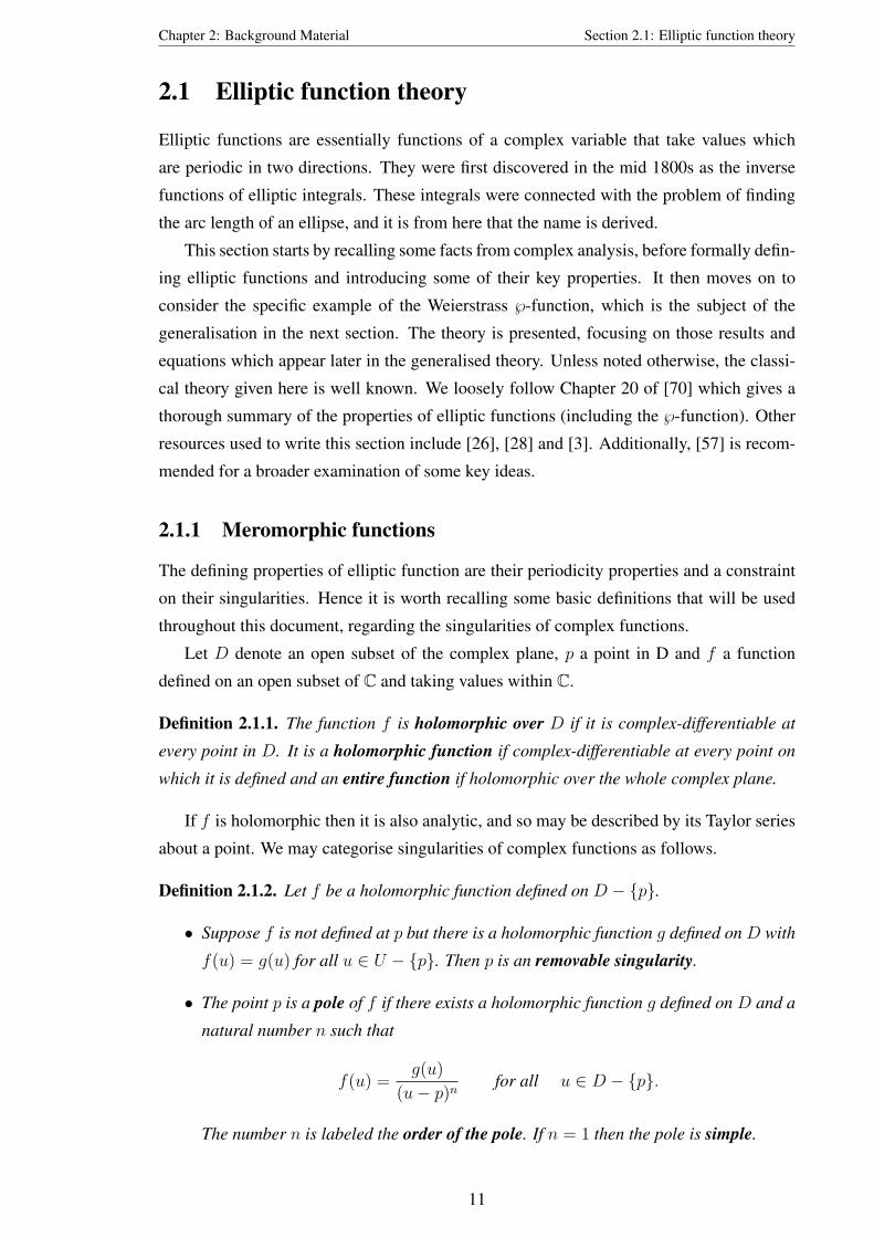
2.1.1 Meromorphic functions
The defining properties of elliptic function are their periodicity properties and a constraint
on their singularities. Hence it is worth recalling some basic definitions that will be used
throughout this document, regarding the singularities of complex functions.
Let D denote an open subset of the complex plane, p a point in D and f a function
defined on an open subset of C and taking values within C.
Definition 2.1.1. The function f is holomorphic over D if it is complex-differentiable at
every point in D. It is a holomorphic function if complex-differentiable at every point on
which it is defined and an entire function if holomorphic over the whole complex plane.
If f is holomorphic then it is also analytic, and so may be described by its Taylor series
about a point. We may categorise singularities of complex functions as follows.
Definition 2.1.2. Let f be a holomorphic function defined on D − p.
• Suppose f is not defined at p but there is a holomorphic function g defined on D with
f(u) = g(u) for all u ∈ U − p. Then p is an removable singularity.
• The point p is a pole of f if there exists a holomorphic function g defined on D and a
natural number n such that
f(u) =g(u)
(u− p)nfor all u ∈ D − p.
The number n is labeled the order of the pole. If n = 1 then the pole is simple.
11

Chapter 2: Background Material Section 2.1: Elliptic function theory
• The point p is an essential singularity if and only if limu→p f(u) does not exist as a
complex number, nor equals infinity. The Laurent series of f at p will have infinitely
many terms of negative degree.
If there exists a disk D centred on p such that f is holomorphic on D − p then p is an
isolated singularity. By definition both removable singularities and poles are isolated. Any
isolated singularity that is not removable or a pole is an essential singularity.
Definition 2.1.3. The function f is meromorphic function on D if it is holomorphic on all
of D except a set of isolated points, which are poles of the function.
Since the poles of a meromorphic function are isolated, they are at most countably
infinite. The function f may be expressed as a Laurent series about p.
f(u) =∞∑
n=−∞
αn(u− p)n, u ∈ C (2.1)
Definition 2.1.4. The constant α−1 is called the residue of f(u). If f is holomorphic at p
then the residue is zero, (although the converse is not always true). At a simple pole, the
residue is given by
Res(f(u), p) = limu→p
(u− p)f(u). (2.2)
2.1.2 Elliptic functions
Definition 2.1.5. An elliptic function is a meromorphic function, f(u), defined on C for
which there exist two periods ω1, ω2.
f(u+ ω1) = f(u+ ω2) = f(u) for all u ∈ C. (2.3)
The periods are non-zero complex numbers that satisfy ω1/ω2 /∈ R.
The periods ω1, ω2 are usually assumed to be the smallest complex numbers in the
second quadrant of the Argand diagram which satisfy equation (2.3). In Figure 2.1 we have
plotted the points 0, ω1, ω2, ω1 + ω2 and joined them up to give a parallelogram. This is
known as the fundamental period parallelogram for the elliptic functions with periods
ω1, ω2. Note that if the ratio, ω1/ω2 was real then the parallelogram would collapse to a
line, and the function would either be a constant, or have just one period.
Copies of this parallelogram can be used to span the complex plane C. Each parallelo-
gram is called a period parallelogram and together they for a mesh over C. (See Figure
2.2.) Two points, say U and U ′, that occur at the same position in the parallelogram are
called congruent. We may write this using the notation,
U ≡ U ′ (mod ω1 + ω2).
12

Chapter 2: Background Material Section 2.1: Elliptic function theory
Note that an elliptic function will take the same value at congruent points.
Figure 2.1: The fundamental period parallelogram formed by ω1 and ω2.
Figure 2.2: A mesh of period parallelograms. The points U , U ′ and U ′′ are congruent, soan elliptic function would take the same value at these points.
For integration purposes it is not convenient to deal with meshes if they have singu-
larities of the integrand on the boundaries. However, due to the periodicity properties, no
information would be lost if the integral of an elliptic function was taken not over a period
parallelogram, but over one of its translations (without rotation) which we label a cell. The
values assumed by an elliptic function along a cell are a repetition of its values along a
period parallelogram.
In Appendix A.1 a number of interesting and useful results for elliptic functions are
proved. We summarise these below.
13

Chapter 2: Background Material Section 2.1: Elliptic function theory
• An elliptic function has a finite number of poles in each cell.
• An elliptic function has a finite number of zeros in each cell.
• Consider the poles of an elliptic function in a cell. The sum of the residues will be
zero.
• An elliptic function with no poles is a constant.
• There does not exist an elliptic function with a single simple pole.
• A non-constant elliptic function has exactly as many poles as zeros (when counting
multiplicities).
• If f(u) is an elliptic function and c a constant then the number of roots of f(u) = c in
any cell is the number of poles of f(u) in a cell. This number is defined as the orderof the elliptic function.
• Let a1, . . . , an denote the zeros and b1, . . . , bn the poles of an elliptic function (when
counting multiplicities). Then
a1 + · · ·+ an ≡ b1 + · · ·+ bn (mod ω1 + ω2) (2.4)
Types of elliptic functions
The two standard forms of elliptic functions are the Jacobi elliptic functions and the Weier-
strass elliptic functions. The generalisation given in the next section is based on the ℘-
function of Weierstrass and so the rest of this section is dedicated to the study of this.
For a short summary of Jacobi’s approach see Chapter 21 of [70], while a clear detailed
description may be found in [54]. The three basic functions, denoted cn(u), dn(u) and
sn(u) arise from the inversion of the elliptic integral of the first kind. They are doubly
periodic generalisations of the three main trigonometric functions. (See Figure 2.3). While
they are still used in a wide variety of applications, they are not convenient for generalising
the theory.
It is easy to switch between the notation of the Jacobi and Weierstrass approaches using
θ-functions, another component of Jacobi’s theory. While the Jacobi elliptic functions are
not easy to generalise, the θ-functions are and the generalised θ-functions are used to prove
parts of the general theory in the next section. The definitions and core properties of the
Jacobi θ-functions are summarised in Appendix A.2. It may be possible to use θ-functions
as an alternative to the Weierstrass function approach of this document, however they are
not considered as advantageous.
14

Chapter 2: Background Material Section 2.1: Elliptic function theory
One of the major benefits of the Weierstrass ℘-functions is that the pole structure is as
simple as possible, with one double pole in each cell. (Recall from Theorem A.1.1 that a
holomorphic elliptic function is a constant and there does not exist an elliptic function with
a single simple pole). Further, these poles occur exactly at the corners of the period paral-
lelograms. See Figure 2.4 for a comparison of a Jacobi elliptic function with a Weierstrass
elliptic function. Note that the Weierstrass ℘-function and its first derivative span the field
of elliptic functions and so the theory of elliptic functions may be constructed using only
these.
Visualising elliptic functions
The plots displayed over the coming pages were obtained from [55] and give visualisations
of periodic complex functions. They are included to clarify some of the points made earlier
in this section. Each plot is a square in the complex plane centred at the origin with corners
at±6± 6i. The blue regions indicate where the function in question has positive imaginary
part, while the red regions are where it has negative imaginary part. Along the boundaries of
these regions the function takes real values. The white lines indicate that the real part of the
function is zero, while the grey grid lines are lines of constant real or imaginary parts. Since
the functions are periodic the patterns will continue to repeat outside the region shown.
Figure 2.3: Comparison of a trigonometric function with an elliptic function
(a) The sine function (b) A Jacobi sn-function
In Figure 2.3 we compare a trigonometric function with an elliptic function. The val-
ues given by both the sine and sn-function repeat as the real part of the input variable is
increased or decreased. Hence the pattern in the plots repeats in the horizontal direction.
The sn-function will also repeat in the vertical direction as the imaginary part is varied.
15

Chapter 2: Background Material Section 2.1: Elliptic function theory
The plots are very similar close to the real axis, but differ in the rest of the complex
plane. Changing from sin(u) to sn(u) causes the vertical edges of the strips to bend inward
and enclose rectangles. Where the tips meet, the function has simple poles, as indicated by
rapid change in grid lines.
In Figure 2.4 we compare a Jacobi elliptic function with a Weierstrass elliptic function.
Both of these functions are elliptic and hence the patterns repeat in two different directions
due to the double periodicity.
Note that these plots of elliptic function are given for specific values of the periods.
The patterns and values the function take may change with different periods, but the core
properties do not.
In each of the plots a black line has been drawn around a cell (region which repeats over
C). Note that in each cell the Jacobi function has two simple poles, while the Weierstrass
function has a single double pole.
Figure 2.4: Comparison of a Jacobi elliptic function with a Weierstrass elliptic function
(a) A Jacobi sn-function (b) A Weierstrass ℘-function
Finally, in Figure 2.5, we compare two different special cases of the Weierstrass ℘-
function. The difference arises from the values of the two periods which were used. In the
first plot it can be seen that the period parallelograms are in fact squares. In the second plot
the period parallelograms are made up from two equilateral triangles. This is not as clear
from the plot and so in each case the fundamental period parallelogram has been marked
on in black.
16

Chapter 2: Background Material Section 2.1: Elliptic function theory
Figure 2.5: Comparison of two different Weierstrass ℘-functions
(a) The lemniscatic ℘-function (b) The equianharmonic ℘-function
Note that although the patterns are differ-ent, the pole properties remain the same.That is, the only singularities are doublepoles at the corners of the period parallel-ograms.The third plot is the derivative of the func-tion used for the second plot. It shows thetriangles that make up the period parallel-ograms more clearly. The derivative hastriple poles on the parallelogram corners.
(c) The derivative of the equianharmoniccccc℘-function
2.1.3 The Weierstrass ℘-function
As with an arbitrary elliptic function the ℘-function is defined using a complex variable
u and two complex periods ω1, ω2. There are several alternative definitions which can
be given. The definition given below is probably the most common, although it will be
equation (2.21) that is extended in the next section to give a definition for the higher genus
℘-functions. When dealing with problems that require numerical results then it is most
efficient to use the definition for the ℘-function in terms of θ-functions. These are discussed
in Appendix A.2 with the definition given by equation (A.13).
17

Chapter 2: Background Material Section 2.1: Elliptic function theory
Definition 2.1.6. The Weierstrass ℘-function with respect to the periods ω1, ω2 is given by
℘(u) = ℘(u;ω1, ω2) =1
u2+
∑m,n∈Z
m2+n2 6=0
1
(u−mω1 − nω2)2− 1
(mω1 + nω2)2
.
Remark 2.1.7.
(i) The infinite double sum in the definition has m,n ranging over the integers, with the
entry where n = m = 0 excluded. For simplicity the notation∑′
m,n is often used to
denote this.
(ii) Note that if n,m 6= 0 thenmω1 +nω2 6= 0. (If this were not the case then n = −mω1
ω2.
But recall from Definition 2.1.5 that ω1
ω2/∈ R. Hence there is a contradiction since
n,m ∈ Z.)
(iii) It is now clear that ℘(u) is holomorphic for all values of u ∈ C except those equal
to mω1 + nω2 for some n,m. At these points the function has a double pole. Hence
℘(u) is meromorphic.
Definition 2.1.8. Denote the period lattice formed from ω1, ω2 by Λ. This is the set of points
Λm,n = mω1 + nω2, m, n ∈ Z.
This can be used to simplify the definition of ℘(u) to
℘(u) = ℘(u; Λ) = u−2 +′∑
m,n
[(u− Λm,n)−2 − Λ−2
m,n
]. (2.5)
This series defining ℘(u) is absolutely and uniformly convergent (see Chapter 3.4 in
[70]), and is constructed from entire functions. Hence it is appropriate to use term by term
differentiation to define the derivatives of the ℘-function. We use the prime notation to
indicate the first derivative of the ℘-function with respect to its variable.
℘′(u) =d
du℘(u) = −2u3 − 2
′∑m,n
(u− Λm,n)−3
= −2∑m,n
(u− Λm,n)−3. (2.6)
Lemma 2.1.9. The function ℘′(u) is odd: ℘′(−u) = −℘′(u).
18

Chapter 2: Background Material Section 2.1: Elliptic function theory
Proof. Consider
℘′(−u) = −2∑m,n
(−u− Λm,n)−3 = 2∑m,n
(u+ Λm,n)−3.
−℘′(−u) = −2∑m,n
(u+ Λm,n)−3.
The set of points −Λm,n is the same as the set Λm,n and so the terms in −℘(−u) will be
the same as those in ℘(u) except in a different order. Now since the series for ℘′(u) is
absolutely convergent the order will not matter, and hence ℘′(u) is odd.
Lemma 2.1.10. The function ℘(u) is even: ℘(−u) = ℘(u).
Proof. The proof is in an identical manner to the previous lemma.
Lemma 2.1.11. The function ℘′(u) is doubly periodic with respect to ω1, ω2.
Proof. Consider
℘′(u+ ω1) = −2∑m,n
(u− Λm,n + ω1)−3.
The set of points Λm,n + ω1 is the same as the set Λm,n so the series for ℘′(u + ω1) is a
rearrangement of the series for ℘′(u). Hence, since the series is convergent,
℘′(u+ ω1) = ℘′(u). (2.7)
So ℘′(u) has period ω1 and using an identical method also period ω2.
Lemma 2.1.12. The function ℘(u) is doubly periodic with respect to ω1, ω2.
Proof. Integrate equation (2.7) to give ℘(u+ ω1) = ℘(u) + A. Substitute in
u = −ω1
2to give ℘
(ω1
2
)= ℘
(−ω1
2
)+ A.
Recall that ℘(u) is even and hence A = 0. Therefore ℘(u) is periodic with period ω1. An
identical method shows it is also periodic with period ω2.
Remark 2.1.13. From Remark 2.1.7 we know ℘(u) is a meromorphic function and it has
just been shown in Lemma 2.1.12 that it is periodic with respect to ω1, ω2. Hence by
Definition 2.1.5, ℘(u) is an elliptic function.
Similarly, from equation (2.6) it can be seen that ℘′(u) is homomorphic everywhere
except its poles and is hence meromorphic. Coupled with Lemma 2.1.11 this allows us to
conclude that ℘′(u) is an elliptic function.
19

Chapter 2: Background Material Section 2.1: Elliptic function theory
The differential equation satisfied by ℘(u)
The Weierstrass ℘-function satisfies a differential equation linking the function with its first
derivative. This equation can be used to specify the function and is the core of several
applications. The equation can be derived by considering the series expansion of the ℘-
function.
Theorem 2.1.14. The function ℘(u) satisfies
[℘′(u)]2 = 4℘(u)3 − g2℘(u)− g3, (2.8)
where g2 and g3 are defined as the elliptic invariants and are given by
g2 = 60′∑
m,n
Λ−4m,n, g3 = 140
′∑m,n
Λ−6m,n. (2.9)
Proof. Consider the function, f(u) = ℘(u)− u−2. From equation (2.5)
f(u) =′∑
m,n
[(u− Λm,n)−2 − Λ−2
m,n
]. (2.10)
Using Lemma 2.1.10 the function f(u) can be concluded even. It will be holomorphic in a
region about the origin and so Taylor’s theorem may be applied here. (Recall that an even
function will have an Taylor series expansion with only even powers.)
f(u) = f(0) +f ′′(0)
2!u2 +
f (4)(0)
4!u4 +O(u6).
From equation (2.10) it is obvious that f(0) = 0. Differentiating gives
f ′′(u) = −6′∑
m,n
[u− Λm,n]−4, =⇒ f ′′(0) = 6′∑
m,n
Λ−4m,n,
f (4)(u) = −120′∑
m,n
[u− Λm,n]−6, =⇒ f (4)(0) = 120′∑
m,n
Λ−6m,n.
Then substituting back gives
f(u) = 3
[′∑
m,n
Λ−4m,n
]u2 + 5
[′∑
m,n
Λ−6m,n
]u4 +O(u6)
=1
20g2u
2 +1
28g3u
4 +O(u6),
where
g2 = 60′∑
m,n
Λ−4m,n, g3 = 140
′∑m,n
Λ−6m,n.
20

Chapter 2: Background Material Section 2.1: Elliptic function theory
So the series expansion for ℘(u) is
℘(u) = u−2 + 120g2u
2 + 128g3u
4 +O(u6). (2.11)
Differentiating term by term gives a similar series for ℘′(u).
℘′(u) = −2u−3 + 110g2u+ 1
7g3u
3 +O(u5). (2.12)
Respectively cube and square these results to get
℘(u)3 = u−6 + 320g2u
−2 + 328g3 +O(u2),
[℘′(u)]2 = 4u−6 − 25g2u
−2 − 47g3 +O(u2).
Hence
[℘′(u)]2 − 4℘(u)3 = −g2u−2 − g3 +O(u2).
Then, using equation (2.11),
[℘′(u)]2 − 4℘(u)3 + g2℘(u) + g3 = O(u2).
This means that the function on the left hand side is holomorphic at the origin. Further,
this function is constructed from elliptic functions, and so is elliptic itself. The function is
holomorphic at all points congruent to the origin, however these are the only possible singu-
larities. Therefore this is an elliptic function with no singularities and by Theorem A.1.1(v)
is a constant. Finally, since the expansion of the function is O(u2), this constant must be
set to zero.
[℘′(u)]2 − 4℘(u)3 + g2℘(u) + g3 = 0.
Therefore ℘(u) satisfies the differential equation given in the theorem for the given values
of g2, g3.
Corollary 2.1.15. The Weierstrass ℘-function satisfies
℘′′(u) = 6℘(u)2 − 12g2. (2.13)
Proof. Differentiate equation (2.8) derived above with respect to u.
2℘′(u)℘′′(u) = 12℘(u)2℘′(u)− g2℘′(u).
Then dividing both sides by 2℘′(u) will give the desired result.
21

Chapter 2: Background Material Section 2.1: Elliptic function theory
Corollary 2.1.16. Consider the differential equation(d
dzy(z)
)2
= 4y(z)3 −G2y(y)−G3(y).
A solution is given by
y = ℘(±z + α), α constant,
provided that periods ω1, ω2 can be determined such that G2 and G3 equal the elliptic
invariants as given in equation (2.9).
Proof. Let y = ℘(±z + α) and consider(d
dzy(z)
)2
=((±1)℘′(±z + α)
)2= ℘′(±z + α)2.
Now apply Theorem 2.1.14 to conclude(d
dzy(z)
)2
= 4℘(±z + α)3 − g2℘(±z + α)− g3 = 4y(z)3 −G2y(z)−G3
as required.
Note that so long as G32 6= 27G2
3 it will be possible to find periods ω1, ω2 such that G2
and G3 equal the elliptic invariants. (See Chapter 21.73 in [70].) This result can be used to
derive the following integral formula for the ℘-function.
Lemma 2.1.17. The equation
u =
∫ ∞ξ
(4t3 − g2t− g3
)− 12 (2.14)
is equivalent to the statement ξ = ℘(u).
Proof. Differentiate equation (2.14) with respect to ξ.
du
dξ=(4ξ3 − g2ξ − g3
)− 12 , =⇒
(dξ
du
)2
= 4ξ3 − g2ξ − g3.
From Corollary 2.1.16 above, this gives ξ = ℘(±u+α) for some constant α. To determine
α we let ξ → ∞. From equation (2.14) this implies u → 0 and hence α is pole of the
℘-function. Therefore α = Λm,n for some m,n and so
ξ = ℘(±u+ α) = ℘(±u+ Λm,n) = ℘(±u) = ℘(u)
as required.
22

Chapter 2: Background Material Section 2.1: Elliptic function theory
This result is sometimes abbreviated to
u =
∫ ∞℘(u)
(4t3 − g2t− g3)−12dt. (2.15)
Elliptic curves
Much of the theory of elliptic functions is linked to the properties of a certain class of
algebraic curves, which is introduced below.
Definition 2.1.18. An elliptic curve is a non-singular algebraic curve which may be written
in the form
y2 = x3 + ax+ b. (2.16)
We may instead consider a general cubic polynomial on the right. However, as long as
it has no repeated roots, we can make a change of variables to obtain equation (2.16).
We now demonstrate the link between elliptic curves and elliptic functions. Substitute
x for 413 x in equation (2.16) to obtain
y2 = 4(x)3 + 413ax+ b.
By Corollary 2.1.16 one solution will be y = ℘(u+α) providing periods can be determined
so that the invariants g2, g3 are equal to 413a, b respectively. (Note that this condition will
always be satisfied due to a condition on a and b arising from the curve being non-singular.)
Hence the elliptic curve may be parameterised by the Weierstrass ℘-function.
It is well known that the surface mapped by an elliptic curve is topologically a torus. In
fact, the Weierstrass ℘-function describes how to get from a torus giving the solutions of an
elliptic curve to the algebraic form of the elliptic curve. A torus, T , may be expressed as
the quotient of the complex plane and a lattice, Λ.
T = C/Λ.
(The complex plane with those points at the same position of the lattice ‘glued together’).
Then this torus may be embedded in the complex projective plane by means of the map
u 7→(1, ℘(u; Λ), ℘′(u; Λ)
).
Given an elliptic curve with equation y2 = 4x3 − g2x − g3, equation (2.15) could be
rewritten as
u =
∫ ∞℘(u)
dx
y. (2.17)
23

Chapter 2: Background Material Section 2.1: Elliptic function theory
2.1.4 Weierstrass’ quasi-periodic functions
Weierstrass defined other functions within his theory which were associated to the period
lattice Λ. While these functions are not elliptic they do satisfy quasi-periodic properties
which are demonstrated below. The σ-function in particular plays an important role both in
the elliptic case and in the generalisation of the next section.
Definition 2.1.19. The Weierstrass σ-function and the Weierstrass ζ-function are defined
below using the complex variable u and the period lattice Λ.
σ(u) = σ(u; Λm,n) = u′∏
m,n
[(1− u
Λm,n
)exp
(u
Λm,n
+1
2
[u
Λm,n
]2)]
. (2.18)
ζ(u) = ζ(u; Λm,n) =1
u+
′∑m,n
[1
u− Λm,n
+1
Λm,n
+u
Λ2m,n
]. (2.19)
As discussed in Remark 2.1.7 the ′ means the term in the series withm = n = 0 is excluded.
From these definitions it is clear that σ(u) is an entire function, with simple zeros at
each of the points Λm,n. These are key properties of the function which are present in the
generalisation. The ζ-function is holomorphic everywhere except at the points Λm,n, which
are simple poles of the function. Both these series are absolutely and uniformly convergent.
Lemma 2.1.20. Both ζ(u) and σ(u) are odd functions of u.
Proof. First consider the ζ-function.
−ζ(−u) =1
u+
′∑m,n
[1
u+ Λm,n
+1
Λm,n
+u
Λ2m,n
]
= ζ(u)−′∑
m,n
[1
u− Λm,n
]+
′∑m,n
[1
u+ Λm,n
]
Both the sums on the final line run over all the integers, and so consist of the same terms in
a different order. Since the series is absolutely convergent the two sums can be concluded
equal and hence the ζ-function is odd.
Next consider the σ-function.
σ(−u) = −u′∏
m,n
[(1 +
u
Λm,n
)exp
(− u
Λm,n
+1
2
[− u
Λm,n
]2)]
.
−σ(−u) = u
′∏m,n
[(1 +
u
Λm,n
)exp
(− u
Λm,n
+1
2
[u
Λm,n
]2)]
.
Once again, this infinite product will have the same terms as σ(u) but in a different order
and so the σ-function can be concluded to be odd.
24

Chapter 2: Background Material Section 2.1: Elliptic function theory
Lemma 2.1.21. The Weierstrass functions are connected as follows.
d
dulog[σ(u)
]= ζ(u),
d
duζ(u) = −℘(u). (2.20)
Proof. Taking logs of equation (2.18) gives
log[σ(u)
]= log(u) +
′∑m,n
[log
(1− u
Λm,n
)+
u
Λm,n
+1
2
(u
Λm,n
)2].
Then differentiate once to show
d
dulog[σ(u)
]=
1
u+
′∑m,n
[(Λm,n
Λm,n − u
)(−1
Λm,n
)+
1
Λm,n
+u
Λ2m,n
]
=1
u+
′∑m,n
[(1
u− Λm,n
)+
1
Λm,n
+u
Λ2m,n
]= ζ(u),
as required. Now differentiate again to obtain the second result.
d
duζ(u) = − 1
u2+
′∑m,n
[−1
(u− Λm,n)2+
1
Λ2m,n
]= −℘(u).
Corollary 2.1.22. From the previous lemma it is obvious that
℘(u) = − d2
du2log[σ(u)
]. (2.21)
In the next section it is the σ-function that is generalised first. Then the ℘-functions are
defined by satisfying a generalisation of equation (2.21).
Quasi-periodicity properties
Next the quasi-periodicity properties of these functions are derived from the periodicity
property of ℘(u) given in Lemma 2.1.12. First, integrate ℘(u+ ω1) = ℘(u) to give
ζ(u+ ω1) = ζ(u) + η1,
where η1 is a constant of integration. Substitute u = −ω1
2into the previous equation to find
ζ(ω1
2
)= ζ
(−ω1
2
)+ η1.
Then use the fact that ζ(u) is odd to give
η1 = 2ζ(ω1
2
).
25

Chapter 2: Background Material Section 2.1: Elliptic function theory
Similarly,
ζ(u+ ω2) = ζ(u) + η2 where η2 = 2ζ(ω2
2
).
Theorem 2.1.23 (Legendre’s Formula). The formula η1ω2 − η2ω1 = 2πi is satisfied by
these functions.
Proof. Consider∫Cζ(u)du where C is the boundary of the cell. There is one pole inside
each cell, with residue +1. Hence∫Cζ(u)du = 2πi by Cauchy’s residue theorem. Now
split up the integral to the four sides as discussed in Theorem A.1.1(iii) to find
2πi =
∫ t+ω1
t
[ζ(u)− ζ(u+ ω2)
]du−
∫ t
t+ω2
[ζ(u)− ζ(u+ ω1)
]du
= −η2
∫ t+w1
t
dt+ η1
∫ t+ω2
t
dt = η1ω2 − η2ω1.
Next the quasi-periodicity of σ(u) is derived by integrating the property for the ζ-function.∫ζ(u+ ω1)du =
∫ [ζ(u) + η1
]du
log[σ(u+ ω1)] = log[σ(u)] + η1u+ k =⇒ σ(u+ ω1) = c · eη1uσ(u).
Here k was the constant of integration and c = ek. To find c first set u = −ω1
2,
σ(ω1
2
)= c · e−η1
ω12 σ(−ω1
2
).
Then recall that σ(u) is an odd function to give
c = −eη1ω1/2.
This can be repeated for ω2 giving the following quasi-periodicity properties for σ(u).
σ(u+ ωi) = − exp
[η1
(u+
ωi2
)]σ(u), i = 1, 2. (2.22)
The generalised σ-function is defined later to satisfy an analogue of this property.
Series expansions
As an entire function, σ(u) can be expressed using its Taylor expansion. The derivation
of such an expansion plays a key role in the following chapters and is a powerful tool in
the investigation of the generalised theory. The series expansion in the elliptic case can be
derived easily using the Laurent expansion for ℘(u) that was constructed earlier and given
26

Chapter 2: Background Material Section 2.1: Elliptic function theory
in equation (2.11).
℘(u) = u−2 + 120g2u
2 + 128g3u
4 +O(u6).
Integrating and changing signs gives an expansion for the ζ-function.
ζ(u) = u−1 − 160g2u
3 − 1140g3u
5 −O(u7).
Integrate again and take exponents to give the expansion for the σ-function.
σ(u) = exp[
log(u)− 1240g2u
4 − 1840g3u
6 −O(u8)]
= u · exp[− 1
240g2u
4 − 1840g3u
6 −O(u8)].
We then use the expansion for the exponential function, ex = 1 + x+ x2
2+O(x3), to show
σ(u) = u− 1240g2u
5 − 1840g3u
7 +O(u9). (2.23)
In fact, both the elliptic ℘ and σ-functions can be given as power series with coefficients
that satisfy a recursive argument. The σ-function can be given by the double sum,
σ(u) =∞∑
m,n=0
am,n
(1
2g2
)m (2g3
)n u4m+6n+1
(4m+ 6n+ 1)!, (2.24)
where a0,0 = 1 and am,n = 0 for either m or n negative. The other values are given by the
recurrence relation
am,n = 3(m+ 1)am+1,n+1 +16
3(n+ 1)am−2,n+1
− 1
3(2m+ 3n− 1)(4m+ 6n− 1)am−1,n.
Similarly, the Laurent expansion of ℘(u) at u = 0 can be given by
℘(u) =1
u2+∞∑n=1
bnu2n, where b1 =
g2
20, b2 =
g3
28
and bn =3
(2n+ 3)(n− 2)
n−2∑k=1
bkbn−k−1, for n > 2.
(See for example [26] page 30.)
Building blocks of elliptic functions
The generalisation of the σ-function will play a key role in the following chapters. One of
the main reasons for this is that any Abelian function can be expressed using σ-functions
with the same periods. We prove this now for the elliptic case.
27

Chapter 2: Background Material Section 2.1: Elliptic function theory
Theorem 2.1.24. Any elliptic function f(u) can be expressed as a quotient of σ-functions
with the same periods as follows.
f(u) = K ·n∏r=1
σ(u− ar)σ(u− br)
, (2.25)
where a1, . . . , an are the set of irreducible zeros of the function, b1, . . . , bn are a set of poles
of f(u) such that all poles of f(u) are congruent to one of them, and K is a constant.
Proof. This proof follows Section 20.53 of [70]. Suppose f(u) is an elliptic function with
periods ω1, ω2 as normal. By Theorem A.1.1(ii) there will be a finite set of irreducible zeros
of f(u), labeled here as a1, . . . , an. By Theorem A.1.3 there will be a set of poles b1, . . . , bn
such that all poles of f(u) are congruent to one of them. (Recall that poles and zeros are
counted according to multiplicity). Further by Theorem A.1.5,
a1 + · · ·+ an = b1 + · · ·+ bn. (2.26)
Now, consider the function
g(u) =n∏r=1
σ(u− ar)σ(u− br)
.
The function g(u) will clearly have the same poles and zeros as f(u). Consider the effect
of increasing u by ω1.
g(u+ ω1) =n∏r=1
σ(u− ar + ω1)
σ(u− br + ω1)=
n∏r=1
exp[(u− ar + ω1
2)η1]
exp[(u− br + ω1
2)η1]
σ(u− ar)σ(u− br)
=
[n∏r=1
exp[u− ar + ω1
2]
exp[u− br + ω1
2]
][n∏r=1
σ(u− ar)σ(u− br)
].
However
n∏r=1
exp[u− ar + ω1
2]
exp[u− br + ω1
2]
=n∏r=1
exp(u) exp(−ar) exp(ω1
2)
exp(u) exp(−br) exp(ω1
2)
=n∏r=1
exp[−ar]exp[−br]
=exp[−(a1 + · · ·+ ar)]
exp[−(b1 + · · ·+ br)]= 1,
where the final equality follows from equation (2.26). Hence g(u+ω1) = g(u) and similarly
for ω2. Finally consider the quotient,f(u)
g(u).
This is is an elliptic function with no zeros or poles. By Theorem A.1.1(v) it is a constant,
say K. Therefore the arbitrary elliptic function f(u) can be expressed in the form
f(u) = K ·n∏r=1
σ(u− ar)σ(u− br)
,
28

Chapter 2: Background Material Section 2.1: Elliptic function theory
as required.
2.1.5 The addition formulae
One of the most celebrated features of the Weierstrass ℘-function is that it satisfies an addi-
tion formula. That is, ℘(u+ v) can be expressed as a rational function of ℘(u), ℘(v), ℘′(u)
and ℘′(v) for general u, v.
Theorem 2.1.25. The following addition formula is true for two arbitrary complex vari-
ables u, v such that u 6= ±v mod(ω1 + ω2).
℘(u+ v) =1
4
[℘′(u)− ℘′(v)
℘(u)− ℘(v)
]2
− ℘(u)− ℘(v). (2.27)
If u = ±v mod(ω1 + ω2), but 2u is not a period then the following duplication formula is
satisfied.
℘(2u) =1
4
[℘′′(u)
℘′(u)
]2
− 2℘(u). (2.28)
Proof. Consider the equations
℘′(u) = A℘(u) +B, ℘′(v) = A℘(v) +B (2.29)
and solve simultaneously to give
A =℘′(u)− ℘′(v)
℘(u)− ℘(v). (2.30)
This is valid for u 6= ±v mod(ω1 + ω2) which was specified in the theorem. Next consider
the function below, defined with this same A,B.
f(κ) = ℘′(κ)− A℘(κ)−B.
The function f(κ) is clearly elliptic, with a triple pole at κ = 0. Therefore by Theorem
A.1.3 the function has three zeros and by Theorem A.1.5 the sum of these will be zero, (the
sum of the poles). From equations (2.29) it can easily be seen that κ = u and κ = v are
zeros of f(κ). Then since the sum is zero the third zero must be κ = −u− v.
Next consider the function
g(κ) = ℘′(κ)2 − [A℘(κ) +B]2.
When κ is congruent to u, v or −u− v,
f(κ) = 0 =⇒ ℘′(κ) = A℘(κ) +B =⇒ ℘′(κ)2 =[A℘(κ) +B
]2,
29

Chapter 2: Background Material Section 2.1: Elliptic function theory
and so at these points the function g(κ) will vanish. Expanding the bracket and using the
differential equation for the ℘-function, (2.8), gives
g(κ) = 4℘(κ)3 − A2℘(κ)2 − (2AB + g2)℘(κ)− (B2 + g3),
which vanishes when ℘(κ) is equal to any one of ℘(u), ℘(v) or ℘(u + v). For general u, v
these are unequal and so they are all roots of the general equation
4X3 − A2X2 − (2AB + g3)X − (B2 + g3) = 0.
Now, recall that in general the sum of the roots of a cubic equation is given by −c2/c3,
where c3 and c2 are the coefficients of the cubic and quadratic terms respectively. Therefore
℘(u) + ℘(v) + ℘(u+ v) = 14A2.
Finally, substituting from equation (2.30) and rearranging give the desired addition formula.
℘(u+ v) =1
4
[℘′(u)− ℘′(v)
℘(u)− ℘(v)
]2
− ℘(u)− ℘(v)
To derive the duplication formula take the limit when v approaches u.
limv→u
℘(u+ v) =1
4limv→u
[℘′(u)− ℘′(v)
℘(u)− ℘(v)
]2
− ℘(v)− limv→u
℘(v).
So long as 2u is not a period, this will reduce to
℘(2u) =1
4limh→0
[℘′(u)− ℘′(u+ h)
℘(u)− ℘(u+ h)
]2
− 2℘(u).
Now apply Taylor’s theorem to ℘(u+ h) and ℘′(u+ h).
℘(2u) =1
4limh→0
[−h℘′′(u) +O(h2)
−h℘′(u) +O(h2)
]2
− 2℘(u).
Therefore, so long as 2u is not a period,
℘(2u) =1
4
[℘′′(u)
℘′(u)
]2
− 2℘(u)
as required.
These addition and duplication formulae for the ℘-function are in fact the algebraic form
of the addition law that can be defined for points on an elliptic curve. It is this property of
elliptic curves which makes them so important in areas such as cryptography. For a detailed
30

Chapter 2: Background Material Section 2.1: Elliptic function theory
description of elliptic curves from the perspective of their use in cryptography see [67].
Additionally, [27] gives full details of how such schemes are implemented and details of
similar properties for the hyperelliptic generalisation discussed in Section 2.3.1.
Now we consider the corresponding addition formula for the σ-function.
Theorem 2.1.26. The following addition formula holds for any two complex variables u, v.
−σ(u+ v)σ(u− v)
σ(v)2σ(u2)= ℘(u)− ℘(v). (2.31)
Proof. Consider the elliptic function
f(u, v) = ℘(u)− ℘(v).
Let us describe this as a function of one variable, z = u+ v,
f(z) = ℘(z − v)− ℘(z − u).
The function f(u, v) will have double poles when u = 0 or v = 0 (and at congruent
points). Equivalently f(z) has double poles at z = u and z = v. Next, f(u, v) will have
zeros when ℘(u) = ℘(v). Clearly this is when v = u and also when v = −u, recalling that
the ℘-function is even. Equivalently the function f(z) has zeros when z = 0 and z = 2v.
Therefore apply the result of Theorem 2.1.24 to give
f(z) = Kσ(z − 0)σ(z − 2v)
σ(z − u)2σ(z − v)2=⇒ f(u, v) = K
σ(u+ v)σ(u− v)
σ(v)2σ(u2)
for some constant K. Returning from z to u, v and recalling our original definition of
f(u, v) gives
℘(u)− ℘(v) = Kσ(u+ v)σ(u− v)
σ(v)2σ(u2).
To determine the constant K use the series expansions given in equations (2.11) and (2.23).
Substituting in the expansions up to order six and expanding gives
0 =(464486400000(1 +K)
)u4v2 −
(464486400000(K + 1)
)u2v4
+ higher degree terms.
Hence we must have K = −1, and so equation (2.31) has been derived as required.
While these addition formulae for the ℘ and σ-functions are related, in the higher genus
cases it will be the σ-function addition formula which can be generalised. In fact it can be
generalised to whole families of addition formula depending on the symmetries present.
31

Chapter 2: Background Material Section 2.2: Abelian function theory
2.2 Abelian function theory
At the end of this section a class of multivariate functions with multiple periods will be
defined. These will be an analogue of the Weierstrass ℘-function, but instead of using two
scalar periods the function will use two matrices of periods. These will be derived from
particular classes of algebraic curves, which give us a framework to classify the functions.
This section first introduces the curves considered and describes how period matrices are
derived from them. We then proceed to define a generalisation of the Weierstrass σ-function
and uses that to define the generalised ℘-functions.
2.2.1 Curves, surfaces and differentials
We will consider the following set of algebraic curves, classified using the notation of [23].
Definition 2.2.1. For two coprime integers (n, s) with s > n we define a general(n, s)-curve as an algebraic curve,
f(x, y) = 0, f(x, y) = yn − xs −∑α,β
µ[ns−αn−βs]xαyβ. (2.32)
In this equation x, y are two complex variables while the µj are a set of curve constants. The
subscripts of these constants are just labels chosen to match the weight properties that are
discussed in Section 3.3. The α and β are integers restricted by α ∈ (0, s−1), β ∈ (0, n−1)
and αn+ βs < ns.
These curves have several properties which make them simpler to work with than an ar-
bitrary algebraic curve. They are non-singular, non-degenerate (have no multiple points)
and have one of their branch points at infinity in the projective plane, (denoted∞). In the
literature these curves are sometimes referred to as canonical curves. (See Chapter 3 of
[35] for some details regarding the theory associated to a less restrictive class of algebraic
curves).
We can think of these curves as compact Riemann surfaces by introducing a local
parametrisation of the curve. We describe the point (x, y) in the vicinity of the point (a, b)
using the local parameter ξ at this point.
(x, y) =
(a+ ξ, b+ ξ
)if (a, b) is a regular point.(
1
ξn,
1
ξs
)if (a, b) = (∞,∞) is a branching point at∞.(
a+ ξm, b+ ξ)
if (a, b) is another branching point of order m.
Recall that Riemann surfaces look like the complex plane locally near every point, but the
global topology can be quite different. They are one dimensional complex manifolds.
32

Chapter 2: Background Material Section 2.2: Abelian function theory
The genus of such a surface is a unique integer associated to the surface which repre-
sents the maximum number of cuts along closed simple curves that can be made without
rendering the resulting manifold disconnected. It is topologically invariant and may be cal-
culated using the degree and singularity properties of the curve. It may be equivalently
thought of as the number of handles of the surface. (See Figure 2.6.)
Figure 2.6: The genus of mathematical surfaces
(a) A surface with genus zero (b) A surface with genus one
(c) A surface with genus two (d) A surface with genus three
From [35] we see that the general (n, s)-curves have genus given by the particularly simple
formula,
g =1
2(n− 1)(s− 1). (2.33)
Throughout this document we will use g to represent the genus of the curve we are working
with. It can be thought informally as a measure of the complexity of the theory. Note that
the classic elliptic curve could be labeled a (2, 3)-curve and has genus one as predicted by
equation (2.33). We now define a subset of the general (n, s) curves obtained by setting
β = 0 in Definition 2.2.1.
Definition 2.2.2. For two coprime integers (n, s) with s > n we define a cyclic(n, s)-curve as an algebraic curve,
f(x, y) = 0, f(x, y) = yn − (xs + λs−1xs−1 + · · ·+ λ1x+ λ0). (2.34)
33

Chapter 2: Background Material Section 2.2: Abelian function theory
In keeping with tradition we use λj for the curve constants in the cyclic case.
We use the name cyclic because these curves are invariant under
[ζ] : (x, y)→ (x, ζy), (2.35)
where ζ is a nth root of unity. The cyclic (n, s)-curve will also have one of its branch
points at ∞ and genus given by equation (2.33). The material presented in this section
is applicable to both the general and cyclic curves. However, it is computationally much
easier to work with the cyclic curves and in later chapters most results are limited to these
cases. For brevity the label (n, s)-curves is used when it is not necessary to specify.
We denote the Riemann surface defined by an (n, s)-curve with C. The key to identify-
ing the properties of these Riemann surfaces and defining the associated period matrices is
the differentials associated to the surfaces. We will describe how these can be derived for
an arbitrary (n, s)-curve using the Weierstrass gap-sequence as a tool.
The Weierstrass gap sequence
Definition 2.2.3. Let (n, s) be a pair of coprime integers such that s > n ≥ 2. Then the
natural numbers not representable in the form
an+ bs where a, b ∈ N = 0, 1, 2, . . . (2.36)
form a Weierstrass gap sequence, Wn,s. The numbers in the sequence are called gaps,
while the numbers that are representable in the form of (2.36) are labeled the non-gaps.
These sequences, first introduced by Weierstrass, are of great importance in several areas of
mathematics. Appendix A.4 proves and demonstrates the core properties of the sequence.
These include the property that the length of Wn,s is g = 12(n− 1)(s− 1), the genus of the
corresponding (n, s)-curve. We usually denote the sequence of non-gaps by W n,s, include
zero as a non-gap and write both sequences in ascending order as below.
Wn,s = ω1, ω2, ω3, . . . , ωg W n,s = 0, w2, w3, . . . .
We summarise the rest of the results proved in Appendix A.4 below.
• An element of the gap sequence w ∈ Wn,s can be expressed as w = −αn+βs where
α, β ∈ Z, α > 0, 0 < β < n. The integers α, β are determined uniquely.
• The maximal element of the sequence, wg, is equal to 2g − 1.
• If w ∈ Wn,s, then (wg − w) /∈ Wn,s.
• If w > w where w ∈ Wn,s and w /∈ Wn,s, then (w − w) ∈ Wn,s.
34

Chapter 2: Background Material Section 2.2: Abelian function theory
• Each element in the gap sequence satisfies i ≤ wi ≤ 2i− 1.
Some examples of Weierstrass gap-sequences are given below.
W2,3 = 1, W2,5 = 1, 3, W3,4 = 1, 2, 5, W3,5 = 1, 2, 4, 7
The differentials associated with C
When working with Riemann surfaces there are traditionally three types of differential 1-
forms that are considered. (See for example [58] or [16] for a more detailed treatment).
• The differentials of the first kind, are the differential 1-forms that are regular every-
where. We refer to them as the holomorphic differentials.
• The differentials of the second kind are meromorphic, with zero residue at each pole.
• The differentials of the third kind are meromorphic with the sum of the residues equal
to zero.
We will first discuss the holomorphic differentials, which are the building blocks of those
functions that are holomorphic on the surface. They can be represented locally at every
point (x, y) on C in the form
du = h(ξ)dξ,
where h is a holomorphic function and ξ the local parameter in the vicinity of (x, y). For
an algebraic curve of genus g there exist exactly g independent holomorphic differentials,
which form a basis. The following proposition, from [35], describes how we can construct
the basis of holomorphic differentials for an arbitrary (n, s) curve using the gap sequence.
Proposition 2.2.4. Let C be an (n, s)-curve of genus g and Wn,s the Weierstrass gap se-
quence generated by (n, s). Then a basis for the space of holomorphic differentials upon
the curve is
dui(x, y) =xPiyQi
fy(x, y)dx, i = 1, . . . , g (2.37)
where Pi, Qi are the integers in the decomposition of the first g non-gaps, (Lemma A.4.1).
nPi + sQi = ωi i = 1, . . . , g.
This basis is sometimes called the standard or canonical basis of holomorphic differentials.
We denote the row vector containing the basis by du = (dui, du2, . . . , dug).
Example 2.2.5. We will construct a basis of holomorphic differentials for the cyclic (3, 4)-
curve which has genus g = 3. In Example A.4.3 the gap sequence was calculated as
W3,4 = 1, 2, 5. Then the first three non gaps can be decomposed as follows.
35

Chapter 2: Background Material Section 2.2: Abelian function theory
w1 = 0 = 0 · 3 + 0 · 4 =⇒ P1 = 0, Q1 = 0
w2 = 3 = 1 · 3 + 0 · 4 =⇒ P2 = 1, Q2 = 0
w3 = 4 = 0 · 3 + 1 · 4 =⇒ P3 = 0, Q3 = 1
The cyclic (3,4)-curve is defined by
f(x, y) = 0, where f(x, y) = y3 − (x4 + λ3x3 + λ2x
2 + λ1x+ λ0). (2.38)
Therefore fy(x, y) = 3y2 and a basis for the space of holomorphic differentials is
du1(x, y) =dx
3y2, du2(x, y) =
xdx
3y2, du3(x, y) =
ydx
3y2.
We now define a particular second kind differential.
Definition 2.2.6. The 2-form Ω((x, y), (z, w)
)on C × C is a fundamental differential of
the second kind if
1. It is symmetric: Ω((x, y), (z, w)
)= Ω
((z, w), (x, y)
)2. The only pole of second order is along the diagonal of C × C (where x = z)
3. It can be expanded in a power series as
Ω((x, y), (z, w)
)=
(1
(ξ − ξ′)2+O(1)
)dξdξ′ as (x, y)→ (z, w)
where ξ and ξ′ are the local coordinates of (x, y) and (z, w).
We will construct a generalisation of Klein’s explicit realisation of the fundamental differ-
ential in Proposition 2.2.8. This generalisation was developed for the (n, s)-curves in [35].
This realisation is used in the Kleinian formula discussed in Section 3.2 and also allows us
to construct a basis for the differentials of the second kind. These are denoted by
drj(x, y) =hj(x, y)
fy(x, y)dx, j = 1, . . . , g (2.39)
and they are determined modulo the space spanned by the du. Denote the row vector
containing this basis by dr = (dr1, dr2, . . . , drg).
Definition 2.2.7. Define the following meromorphic function on C×C, where [ ]w means
that we remove any terms which have negative powers of w.
Σ((x, y), (z, w)
)=
1
(x− z)fy(x, y)·
n∑k=1
yn−k[f(z, w)
wn−k+1
]w
. (2.40)
36

Chapter 2: Background Material Section 2.2: Abelian function theory
Proposition 2.2.8. The fundamental differential of the second kind can be expressed as
Ω((x, y), (z, w)
)= R
((x, y), (z, w)
)dxdz (2.41)
where
R((x, y), (z, w)
)=
∂
∂zΣ((x, y), (z, w)
)+
g∑j=1
duj(x, y)
dx· drj(z, w)
dz. (2.42)
The polynomials hj(x, y) contained within drj(x, y) should be constructed so that Ω satis-
fies the symmetry condition in Definition 2.2.6.
For the proof see for example [30] page 9. This proposition will allow us to write the
fundamental differential of the second kind as
Ω((x, y), (z, w)
)=
F((x, y), (z, w)
)dxdz
(x− z)2fy(x, y)fw(x, y), (2.43)
where F is a polynomial of its variables.
Example 2.2.9. Consider again the cyclic (3,4)-curve defined by equation (2.38). Since the
curve is cyclic, [f(z, w)
wn−k+1
]w
=w3
w3−k+1, k = 1, . . . , 3.
Therefore the function given in Definition 2.2.7 is
Σ((x, y), (z, w)
)=
1
(x− z) · 3y2·
3∑k=1
y3−k w3
w3−k+1=y2 + yw + w2
3y2(x− z).
Hence equation (2.42) becomes
R((x, y), (z, w)
)=
d
dz
(y2 + yw + w2
x− z
)1
3y2+
(h1(z, w) + xh2(z, w) + yh3(z, w)
9y2w2
),
where the polynomials hj have yet to be determined. Note that from the curve equation
wz =1
3w2
(4z3 + 4λ3z
2 + 2λ2z + λ1
),
and so we can evaluate the derivative in R((x, y), (z, w)) and substitute for wz, (along with
any higher powers of w, using the curve equation). We can find the hj by imposing the
symmetry condition on Ω and hence R((x, y), (z, w)).
R((x, y), (z, w)
)= R
((z, w), (x, y)
).
We find that the condition holds for
h1(x, y) = (5x2 + 3xλ3 + λ2)y, h2(x, y) = 2xy, h3(x, y) = x2.
37

Chapter 2: Background Material Section 2.2: Abelian function theory
Note that this set of polynomials is not unique. For example the λ2 term could have been
included in h2 instead of h1, however, this would have made no difference to the end results.
So given these values of hj we see that a basis for the differentials of the second kind
associated to the cyclic (3,4)-curve is given by
dr1(x, y) =y(5x2 + 3xλ3 + λ2)dx
3y2dx,
dr2(x, y) =2xydx
3y2dx, dr3(x, y) =
x2dx
3y2dx.
Further, the fundamental differential of the second kind is given by
Ω((x, y), (z, w)
)=F((x, y), (z, w)
)dxdz
9(x− z)2y2w2,
where F ((x, y), (z, w)) is the following symmetric polynomial
F ((x, y), (z, w)) = (3λ0 + 2z3x+ 3λ3z2x+ 2λ1z + z2x2 + 2λ2zx+ λ1x+ λ2z
2)y
+ 3y2w2 + (3λ0 + 2x3z + 3λ3x2z + 2λ1x+ x2z2 + 2λ2xz + λ1z + λ2x
2)w
In Section 3.1.1 this calculation is performed for the cyclic (4,5)-curve with details of all
the steps shown in full.
2.2.2 Abelian functions
The next step is to describe how period matrices can be generated from these curves. After
that we introduce the notion of a function that is periodic with respect to these matrices —
an Abelian function. This subsection ends with a discussion on the Jacobian of the curve.
This is an important substructure of the curve that has algebraic group properties and can
be described by the associated Abelian functions.
Let C be the surface defied by an (n, s)-curve, and du = (du1, . . . , dug) the vector of
holomorphic differentials defined in the previous section. We will usually denote a point in
Cg by u, a row vector with coordinates (u1, . . . , ug). Any point u ∈ Cg may be written as
u =
g∑i=1
∫ Pi
∞du, (2.44)
where the Pi are a set of g variable points upon C.
Now we must choose a basis of cycles (closed paths) upon the surface C. Denote them
αi, βj, 1 ≤ i, j ≤ g,
38

Chapter 2: Background Material Section 2.2: Abelian function theory
and ensure they have intersection numbers
αi · αj = 0, βi · βj = 0, αi · βj = δij =
1 if i = j
0 if i 6= j. (2.45)
(Note that these cycles are the first homology basis of the Riemann surface.) We now define
the periods associated to the surface as the integrals of the differentials along these paths.
We combine them into the following two g × g period matrices.
ω′ =
(∮αk
du`
)k,`=1,...,g
ω′′ =
(∮βk
du`
)k,`=1,...,g
(2.46)
Note for future use that the matrix (ω′)−1ω′′ is symmetric with
Im((ω′)−1ω′′
)positive definite. (2.47)
(See [19] for details). These matrices play the role of the scalar periods ω1, ω2 in the el-
liptic theory. They are used below to construct the period lattice Λ, defined in analogy to
Definition 2.1.8 from the elliptic case.
Definition 2.2.10. Denote the period lattice formed from ω′, ω′′ by Λ. These are the points
Λ =ω′m+ ω′′n, m,n ∈ Zg
.
We can now give a definition for those function that are periodic with respect to these
matrices, or equivalently, invariant under translations by this period lattice.
Definition 2.2.11. Let M(u) be a meromorphic function of u ∈ Cg. Then M is an Abelianfunction associated with C if
M(u+ ω′m+ ω′′n) = M(u), (2.48)
for all integer column vectorsm,n ∈ Zg.
The Jacobian
Recall that an algebraic variety is the set of solutions to a system of polynomial equations.
An Abelian variety is an algebraic variety that is also an algebraic commutative group. (I.e.
a group law for points in the variety can be defined by regular functions.) Topologically an
Abelian variety is a complex g-handled torus.
Every algebraic curve C of genus g > 1 is associated with an Abelian variety of dimen-
sion g, called the Jacobian of the curve and denoted J . They are associated by means of an
holomorphic map from C to J . Any point in the Jacobian can be generated by a g-tuple of
39

Chapter 2: Background Material Section 2.2: Abelian function theory
points in C. As with any complex torus of dimension g, the Jacobian may be obtained as
the quotient of a g-dimensional complex vector space by a lattice of rank 2g.
Definition 2.2.12. Let C be defined by an (n, s)-curve and Λ the lattice of its periods. Then
the manifold Cg/Λ is the Jacobian of C, denoted by J .
Intuitively speaking, the Jacobian is Cg with those points on equivalent positions in the
lattice ‘glued together’. Let κ denote the quotient map of modulo Λ over C.
κ : Cg → Cg/Λ = J.
Then Λ = κ−1((0, . . . , 0)). Note that the Jacobian of an elliptic curve is isomorphic to the
curve itself. Hence in the elliptic case equation (2.44) simplifies to equation (2.17), with
dx/y as the sole differential in the basis.
Next, the map that is used to move from the curve to the Jacobian is defined.
Definition 2.2.13. For k = 1, 2, . . . define A, the Abel map, as below. This is a map from
the kth symmetric product of the curve to the Jacobian of the curve.
A : Symk(C)→ J
(P1, . . . , Pk) 7→(∫ P1
∞du+ · · ·+
∫ Pk
∞du
)(mod Λ). (2.49)
Here the Pi are points upon the curve C.
When k = 1 the Abel map gives an embedding, or a one dimensional image, of C.
The Jacobi Inversion Problem is, given a point u ∈ J to find the preimage of this point
under the Abel map (2.49). Denote the image of the kth Abel map by W [k]. (For k ≥ g the
image W [k] = J by the Abel-Jacobi theorem.)
The next definition is for the strata of the Jacobian. These spaces decrease in dimension
and are the natural location to work with lower dimensional problems (as is the case in
Chapter 6). First note that we write, [−1](u1, . . . , ug) = (−u1, . . . ,−ug).
Definition 2.2.14. Denote the the kth strata of the Jacobian by Θ[k] and define it as below.
Θ[k] = W [k] ∪ [−1]W [k]. (2.50)
This is also referred in the literature as the kth standard theta subset or kth stratum.
These strata are all subsets of the Jacobian and are arranged as follows.
J = Θ[g] ⊃ Θ[g−1] ⊃ · · · ⊃ Θ[1] ⊃ 0 (2.51)
where 0 is the origin, and in the literature is sometimes assigned to be Θ[0]. When the
(n, s)-curve has n even the process is simplified and W [k] = [−1]W [k] = Θ[k].
40

Chapter 2: Background Material Section 2.2: Abelian function theory
2.2.3 The Kleinian σ-function
In Section 2.2.4 the class of Abelian functions that generalise the Weierstrass ℘-function is
defined. This is done using an auxiliary function which we discuss in this section.
First define two further period matrices, (in addition to those given in equation (2.46)),
by integrating the basis of meromorphic differentials, dr. (This basis was defined in equa-
tion (2.39) and should be explicitly determined through the construction of the fundamental
differential of the second kind detailed in Proposition 2.2.8.)
η′ =
(∮αk
dr`
)k,`=1,...,g
η′′ =
(∮βk
dr`
)k,`=1,...,g
(2.52)
We combine the period matrices into
M =
(ω′ ω′′
η′ η′′
).
The matrix M satisfies
M
(0g −IgIg 0g
)MT = 2πi
(0g −IgIg 0g
), (2.53)
where Ig is the identity matrix of size g and 0g is the zero matrix of size g. Equation (2.53)
is known as the generalised Legendre equation and we refer the reader to page 11 of [19]
for more details.
The Kleinian σ-function will be a function associated to the curve C that generalises the
Weierstrass σ-function discussed in Section 2.1.4. (When C is the classical elliptic curve
then the Kleinian σ-function will equal the classical function.) It will be a function of g
variables where g is the genus of the curve.
σ = σ(u) = σ(u1, u2, . . . , ug).
The function was first introduced by Klein in his research on hyperelliptic functions, (see
Section 2.3.1). This approach is developed for the general (n, s)-curves in [19], [35] and
[60]. The definition was developed so that the function would generalise the classical σ-
function, maintaining those properties that are necessary for the successful development of
the theory of Abelian functions. These conditions were that the function be entire, satisfy a
quasi-periodicity property, have a specific set of zeros and a particular series expansion.
Given these properties it was shown that the Kleinian σ-function could be expressed
using multivariate θ-functions. These are a generalisation of the Jacobi θ-functions, (dis-
cussed in Appendix A.2). The essential definitions and properties that are important for this
document are summarised in Appendix A.3. We refer the reader to [59], [42] and [53] for
41

Chapter 2: Background Material Section 2.2: Abelian function theory
a detailed treatment of the multivariate θ-functions.
In a number of applications authors have developed theory purely in the θ-functions, see
for example [61]. However, the σ-function approach pursued in this document is considered
the most advantageous method for developing the theory of Abelian functions.
We now give the definition for the Kleinian σ-function associated toC using θ-functions
and equivalently as an infinite sum. We then present the key properties that the function
was designed to incorporate. For a more detailed study of the construction and properties
of the multivariate σ-function we refer the reader to [19] and [60].
Definition 2.2.15. Let C be an (n, s)-curve and M the matrix of periods discussed above.
Then the Kleinian σ-function associated to C is defined using a multivariate θ-function
with characteristic [δ] as
σ(u) = σ(u;M) = c exp(
12uη′(ω′)−1uT
)· θ[δ]
((ω′)−1uT
∣∣ (ω′)−1ω′′).
Using Definition A.3.2 for the θ-function, we can write it as an infinite sum.
σ(u) = c exp(
12uη′(ω′)−1uT
)×∑m∈Zg
exp
[2πi
(2.54)
12(m+ δ′)T (ω′)−1ω′′(m+ δ′) + (m+ δ′)T ((ω′)−1uT + δ′′)
].
The θ-function characteristic, [δ], is the 2g vector of half integers
[δ] =
[δ′
δ′′
]
that is related to the Riemann constant with base point ∞. (See Appendix A.3 for the
definitions or [19] for full details). The constant c is dependent upon the curve parameters
and the choice of cycles αi, βi. It is fixed later in Remark 2.2.23.
Remark 2.2.16.
(i) When the (n, s)-curve is chosen to be the classic elliptic curve then the Kleinian σ-
function coincides with the Weierstrass σ-function.
(ii) For brevity we will now just refer to the Kleinian σ-function as the σ-function and
specify if we are referring to the classical function.
(iii) The derivatives of the σ-function with respect to the variables in u are often used and
are referred to as σ-derivatives.
They are denoted in this document by adding subscripts as follows.
σi1,i2,...,in(u) =∂
∂ui1
∂
∂ui2. . .
∂
∂uinσ(u), i1 ≤ · · · ≤ in ∈ 1, . . . , g.
42

Chapter 2: Background Material Section 2.2: Abelian function theory
If appropriate then the commas in the indices may be removed for simplicity.
(iv) If the vector of variables to which we are referring is obvious or not relevant then we
may omit it. For example we may write σij instead of σij(u).
We now summarise the most important properties of the σ-function.
Lemma 2.2.17. The Kleinian σ-function and the σ-derivatives are all entire functions of u
over Cg.
Proof. This is clear from equation (2.54).
Next we make precise the periodicity properties of σ(u).
Lemma 2.2.18. Given u ∈ Cg, denote by u′ and u′′ the unique elements in Rg such that
u = ω′u′ + ω′′u′′.
Let ` represent a point on the period lattice. Then
` = ω′`′ + ω′′`′′ ∈ Λ, `′, `′′ ∈ Zg. (2.55)
For u,v ∈ Cg and ` ∈ Λ, define L(u,v) and χ(`) as follows:
L(u,v) = uT(η′v′ + η′′v′′),
χ(`) = exp[2πi
(`′)T δ′′ − (`′′)T δ′ + 12(`′)T`′′].
Then for all u ∈ Cg, ` ∈ Λ the function σ(u) has the following quasi-periodicity property.
σ(u+ `) = χ(`) exp
[L
(u+
`
2, `
)]σ(u). (2.56)
(Note that if σ(u) = 0 then clearly σ(u + `) = 0 also. Therefore, while the σ-function
itself is not Λ-periodic, the zero set of the function is. )
Additionally, the σ-function is modular invariant:
σ(u; ΥM) = σ(u;M), for Υ ∈ Sp(2g,Z). (2.57)
(Sp(2g,Z) is the group of size 2g symplectic matrices with elements in Z).
Proof. The quasi-periodicity property (2.56) is a classical result, first discussed in [7], that
was fundamental to the original definition of the multivariate σ-function. It is a gener-
alisation of equation (2.22) in the classical case and follows from the properties of the
multivariate θ-function.
43

Chapter 2: Background Material Section 2.2: Abelian function theory
Although both c and the θ-function are not independent of the basis of cycles, the σ-
function is, so long as the restriction (2.45) is satisfied. Such a change is equivalent to
multiplying M by another symplectic matrix.
See [19] or [60] for the construction of the σ-function to satisfy these properties.
Recall that the elliptic σ-function has zeros on each of the lattice points. This is not
the case in general, however, we are still able to specify where the σ-function has its zeros.
(The extra simplicity in the elliptic case is due to the fact that an elliptic curve is isomorphic
to its Jacobian.)
Lemma 2.2.19. The function σ(u) has zeros of order one when u ∈ Θ[g−1]. Further, for
all other u we have σ(u) 6= 0.
Proof. This is a classical result first discussed in [7], generalised in [19] and formalised
with this notation in [14]. The σ-function was defined using a Riemann θ-function with
base point∞. By Corollary A.3.7 the θ-function, and hence the σ-function, would vanish
on the theta divisor, which when generated by this base point coincides with our definition
of Θ[g−1].
Recall that the Weierstrass σ-function was an odd function of the variable u. In general the
Kleinian σ-function has definite parity with respect to the change of variables, u 7→ [−1]u
and is odd or even depending on the choice of (n, s).
Lemma 2.2.20. The σ-function associated with an (n, s)-curve has definite parity which
may be predicted by
σ(−u) = (−1)124
(n2−1)(s2−1)σ(u). (2.58)
Proof. This is Proposition 4(iv) in [60].
Consider the Taylor series expansion of σ(u) about the origin, 0 = (0, . . . , 0). This
will be multivariate in the variables u1, . . . , ug and will also depend on the parameters of
the underlying (n, s)-curve. These were denoted by µs or λs depending on the type of
curve, (Definitions 2.2.1 and 2.2.2). The final property of the σ-function that is presented in
this section allows the part of the expansion that does not depend on the curve parameters
to be specified up to a multiplicative constant.
Theorem 2.2.21. The Taylor series expansion of σ(u) about the origin may be written as
σ(u) = K · SWn,s(u) + terms dependent on curve parameters, (2.59)
where K is a constant and SWn,s the Schur-Weierstrass polynomial generated by (n, s).
44

Chapter 2: Background Material Section 2.2: Abelian function theory
Proof. The result was first stated in [20], with an alternative proof now available in [60].
The Schur-Weierstrass polynomial is a finite polynomial in the variables u that is not
dependent on the curve parameters. Appendix A.5 defines the Schur-Weierstrass polyno-
mial and give details on how it is constructed from the integers (n, s). Some examples are
given below for specific values of (n, s).
W2,3 = u1
W2,5 = 12(−u3
2 + 3u1)
W3,4 = 120
(u53 + 20u1 − 20u2
2u3)
W3,5 = 1448
(u84 + 448u3u
24u2 − 56u2
3u44 − 112u4
3 + 448u22 − 448u4u1)
Remark 2.2.22.
(i) In the elliptic case we have (n, s) = (2, 3) and so the σ-function expansion should
contain only one term, u1 multiplied by a constant that does not depend on the curve
parameters. Check equations (2.23) and (2.24) to see that this was indeed the case.
(In the elliptic case the curve parameters were the elliptic invariants g2, g3.)
(ii) The polynomial SWn,s will have, with respect to the variable ug, a leading term given
by a constant multiplied by
u124
(n2−1)(s2−1)g .
(Note that this is the case in the four examples above). This follows from Proposition
4 of [60] and matches the parity property of the σ-function given in Lemma 2.2.20.
This section concludes by fixing the constant c in the definition of the Kleinian σ-
function.
Remark 2.2.23. We will fix the constant c in Definition 2.2.15 to be the value that makes
K = 1 in Theorem 2.2.21. Some other authors working in this area may instead set
c =( πg
det(w′)
) 12 · 1
D12n
,
where D is the discriminant of the curve C. In general these two choices of c are not
equivalent. However the constant cwill cancel in the definitions of all the Abelian functions
used in this paper, (see Appendix B). Hence almost all results derived in later chapters of
this document are independent of c. (The only exceptions are the two-term addition formula
in Sections 3.6 and 4.1 which we discuss when they occur.)
Note that this choice of c ensures that the Kleinian σ-function matches the Weierstrass
σ-function when the (n, s)-curve is chosen to be the classic elliptic curve.
45

Chapter 2: Background Material Section 2.2: Abelian function theory
2.2.4 The Kleinian ℘-functions
We are now in a position to define the generalisation of the ℘-function. We define it using
the Kleinian σ-function by taking logarithmic derivatives, in analogy to equation (2.21) in
the elliptic case. Since in general there is more that one variable, there will be a num-
ber of possible ℘-functions we can define depending on which variable is chosen for the
differentiation. We introduce some new notation to overcome this ambiguity.
Definition 2.2.24. Define the 2-index Kleinian ℘-functions as
℘ij(u) = − ∂2
∂ui∂ujlog[σ(u)
], i ≤ j ∈ 1, . . . , g. (2.60)
Lemma 2.2.25. The 2-index ℘-functions are meromorphic functions with poles of order
two when σ(u) = 0.
Proof. Expand equation (2.60) to give
℘ij(u) =σi(u)σj(u)− σ(u)σij(u)
σ(u)2. (2.61)
Recall that the σ-function is entire and so ℘ij(u) will be meromorphic, with poles of order
two only when σ(u) = 0.
Lemma 2.2.26. The 2-index Kleinian ℘-functions are Abelian functions.
Proof. We need to prove that ℘ij(u) satisfies the periodicity property (2.48). This is equiv-
alent to proving
℘ij(u+ `) = ℘ij(u), (2.62)
where ` is an arbitrary point on the period lattice as defined in equation (2.55). We can
prove this using the quasi-periodicity property of the σ-function, given in equation (2.56).
First recall the functionL(u,v) defined in Lemma 2.2.18. We will examine the function
L(u+ `2, `) which we label L(u) for simplicity.
L(u) = L
(u+
`
2, `
)=
(u+
`
2
)T (η′`′ + η′′`′′).
Using the subscripts to indicate the components of the vectors and matrices we see
L(u) =
u1 + `1
2...
ug + `g2
T
η′11`′1 + η′12`
′2 + · · ·+ η′1g`
′g + η′′11`
′′1 + η′′12`
′′2 + · · ·+ η′′1g`
′′g
...
η′g1`′1 + η′g2`
′2 + · · ·+ η′gg`
′g + η′′g1`
′′1 + η′′g2`
′′2 + · · ·+ η′′gg`
′′g
=(u1 + `1
2
)(η′11`
′1 + η′12`
′2 + · · ·+ η′1g`
′g + η′′11`
′′1 + η′′12`
′′2 + · · ·+ η′′1g`
′′g
)+ . . .
· · ·+(ug + `g
2
)(η′g1`
′1 + η′g2`
′2 + · · ·+ η′gg`
′g + η′′g1`
′′1 + η′′g2`
′′2 + · · ·+ η′′gg`
′′g
).
46

Chapter 2: Background Material Section 2.2: Abelian function theory
Therefore, the derivatives of L(u) are
Li(u) =∂
∂uiL(u) = η′i1`
′1 + η′i2`
′2 + · · ·+ η′ig`
′g + η′′i1`
′′1 + η′′i2`
′′2 + · · ·+ η′′ig`
′′g ,
Lij(u) =∂
∂ui∂ujL(u) = 0. (2.63)
We can now examine the quasi-periodicity of the first and second σ-derivatives, noting that
the latter simplifies due to equation (2.63).
σ(u+ `) = χ(`) exp[L(u)
]· σ(u)
σi(u+ `) = χ(`) exp[L(u)
]·[Li(u)σ(u) + σi(u)
]σij(u+ `) = χ(`) exp
[L(u)
]·[Li(u)Lj(u)σ(u) + Lj(u)σi(u)
+ Li(u)σj(u) + σij(u)]
(2.64)
Now substitute u for u+ ` in equation (2.61) and use equations (2.64).
℘ij(u+ `) =σi(u+ `)σj(u+ `)− σ(u+ `)σij(u+ `)
σ(u+ `)2
=χ(`)2 exp
[L(u)
]2χ(`)2 exp
[L(u)
]2 ·([
Li(u)σ(u) + σi(u)]·[Lj(u)σ(u) + σj(u)
]σ(u)2
−σ(u) ·
[Li(u)Lj(u)σ(u) + Lj(u)σi(u) + Li(u)σj(u) + σij(u)
]σ(u)2
)
=σi(u)σj(u)− σ(u)σij(u)
σ(u)2= ℘ij(u).
So ℘ij(u) satisfies the periodicity condition and by Lemma 2.2.25 the function is meromor-
phic. Hence it is an Abelian function.
We extend this new notation to define the derivatives of these functions.
Definition 2.2.27. For n ≥ 2 define n-index Kleinian ℘-functions as
℘i1,i2,...,in(u) = − ∂
∂ui1
∂
∂ui2. . .
∂
∂uinlog[σ(u)
], i1 ≤ · · · ≤ in ∈ 1, . . . , g.
Note that the n-index ℘ functions are all independent of the constant c used in the
definition of the σ-function. (See Appendix B for the proof.)
We now use similar techniques to show that these functions are also Abelian.
Lemma 2.2.28. The n-index ℘-functions are meromorphic functions with poles of order n
when σ(u) = 0.
47

Chapter 2: Background Material Section 2.2: Abelian function theory
Proof. Use proof by induction. The statement has already been proved for the case n = 2
in Lemma 2.2.25. Suppose it is true for n = p. Then we could write
℘i1,i2,...,ip(u) =f(u)
σ(u)p
where f(p) is an entire function. Differentiating gives
℘i1,i2,...,ip,ip+1(u) =
σ(u)p[
∂
∂uip+1
f(u)
]+ f(u)
[pσ(u)p−1σip+1(u)
]σ(u)2p
=
σ(u)
[∂
∂uip+1
f(u)
]+ pf(u)σip+1(u)
σ(u)2p−(p−1)=
σ(u)
[∂
∂uip+1
f(u)
]+ pf(u)σip+1(u)
σ(u)p+1.
Since both f(u) and σ(u) are entire functions we know the numerator is entire. Hence the
function has poles of order p + 1 when σ(u) = 0. Therefore, if the statement is true for
n = p then it is true for n = p+ 1 as required.
Lemma 2.2.29. The n-index Kleinian ℘-functions are all Abelian functions.
Proof. Given that equation (2.62) is true we can just differentiate to conclude that all the n-
index ℘-functions satisfy the periodicity condition. Coupled with Lemma 2.2.28 this shows
that the n-index Kleinian ℘-functions are all Abelian.
We now give some remarks on how these functions are related to the Weierstrass ℘-
function.
Remark 2.2.30. Definition 2.2.24 was given as an analogy to equation (2.21) in the elliptic
case. It was remarked earlier that when the (n, s)-curve is chosen to be the classic elliptic
curve then the Kleinian σ-function coincides with the classic σ-function. In this case, since
g = 1, there is only one 2-index Kleinian ℘-function and it coincides with the Weierstrass
℘-function. The only difference would be the notation with
℘11(u) ≡ ℘(u), ℘111(u) ≡ ℘′(u), ℘1111(u) ≡ ℘′′(u).
So to emphasise, 2-index ℘-functions play the role of the classic ℘-function, a 3-index the
role of the first derivative ℘′ and a 4-index the role of the second derivative ℘′′.
Remark 2.2.31.
(i) Both the Weierstrass ℘-function and the Kleinian ℘-functions have poles of order two
when the σ-function is zero. In the elliptic case this occurred on the lattice points, but
in general it occurs for u ∈ Θ[g−1].
48

Chapter 2: Background Material Section 2.2: Abelian function theory
(ii) In the elliptic case the functions ℘′ and ℘′′ had poles of order three and four respec-
tively, occurring again at the lattice points. Similarly the n-index Kleinian ℘-functions
have poles of order n when u ∈ Θ[g−1].
Recall that the Weierstrass ℘-function is an even function of its variable while the derivative
℘′ is odd. A similar property is present for the ℘-functions associated to a general (n, s)-
curve.
Lemma 2.2.32. The n-index ℘-functions have definite parity with respect to the change of
variables u→ [−1]u. The functions are odd if n is odd and even if n is even.
Proof. Recall Lemma 2.2.20 which stated that the σ-function had definite parity. Suppose
first that the σ-function is even. Then the odd index σ-derivatives will be odd functions
while the even index σ-derivatives are even functions.
σ([−1]u) = σ(u) =⇒ −σi([−1]u) = σi(u)
σij([−1]u) = σij(u)
Then consider the effect of the change of variables on ℘ij(u) as given by equation (2.61).
℘ij([−1]u) =σi([−1]u)σj([−1]u)− σ([−1]u)σij([−1]u)
σ([−1]u)2
=(−1)2σi(u)σj(u)− σ(u)σij(u)
σ(u)2= ℘ij(u).
Hence the 2-index ℘-functions would be even. Now suppose that the σ-function is odd.
Then the odd index σ-derivatives will be even functions while the even index σ-derivatives
are odd functions.
σ([−1]u) = −σ(u) =⇒ σi([−1]u) = σi(u)
−σij([−1]u) = σij(u)
Consider again the effect of the change of variables on ℘ij(u).
℘ij([−1]u) =σi([−1]u)σj([−1]u)− σ([−1]u)σij([−1]u)
σ([−1]u)2
=σi(u)σj(u)− (−1)2σ(u)σij(u)
[(−1)σ(u)]2= ℘ij(u).
Therefore, regardless of the parity of the σ-function, the 2-index ℘-functions are even.
It clearly follows from their definition that the n-index ℘-functions must then alternate
between having odd and even parity.
We now give some remarks on the notation used in this document.
49

Chapter 2: Background Material Section 2.2: Abelian function theory
Remark 2.2.33.
(i) From now on we may just refer to the ℘-functions, specifying if we are referring to
the Weierstrass function or to ℘-functions of a particular index.
(ii) The ℘-function indices are usually single digits such as ℘ij . Occasionally commas are
used for clarity, as in ℘i1,...,in .
(iii) The order of the indices is irrelevant. For simplicity we always use ascending numer-
ical order, as indicated in the definitions.
(iv) If the vector of variables to which we are referring is obvious or not relevant then we
may omit it. For example we may write ℘ij instead of ℘ij(u).
Note that as the genus of the curve increases so do the number of associated ℘-functions.
It was noted above that when g = 1 there is only one ℘-function of each index, coincid-
ing with the Weierstrass ℘-function and its derivatives. However, when g = 3 for ex-
ample, there will be six 2-index ℘-functions, ten 3-index ℘-functions and fifteen 4-index
℘-functions.
℘ij = ℘11, ℘12, ℘13, ℘22, ℘23, ℘33
℘ijk = ℘111, ℘112, ℘113, ℘122, ℘123, ℘133, ℘222, ℘223, ℘233, ℘333
℘ijkl = ℘1111, ℘1112, ℘1113, ℘1122, ℘1123, ℘1133, ℘1222, ℘1223, ℘1233, ℘1333,
℘2222, ℘2223, ℘2233, ℘2333, ℘3333
In general, the number of r-index ℘-functions associated with a genus g curve is
(g + r − 1)!
r!(g − 1)!.
(Since the problem is choosing r indices from g possible indices with repetition allowed
and order not important.)
50

Chapter 2: Background Material Section 2.3: Literature review
2.3 Literature review
The definitions of the previous section were given for an arbitrary (n, s)-curve of genus g,
generating infinite classes of Abelian functions with increasing genus. Such a definition was
not developed as an immediate generalisation of the Weierstrass elliptic function theory.
In this section we discuss in chronological order the cases that have been considered. We
present some of the more important results which motivate the work in the coming chapters.
The first generalisation of elliptic functions were labeled hyperelliptic functions and
had two variables and four periods. They could be defined as functions on the Jacobian of
a hyperelliptic curve.
Definition 2.3.1. A hyperelliptic curve is an algebraic curve given by an equation of the
form
y2 = f(x),
where f(x) is a polynomial of degree n > 4 with n distinct roots.
From Definition 2.2.2 all the the cyclic (2, s)-curve are hyperelliptic curves.
There were several alternative approaches taken to developing the theory of hyperellip-
tic functions, before Klein developed the definitions that were generalised in Section 2.2.
These originated from the German language paper, [51]. The following quote is taken from
the introduction of [19], with the citations replaced with the numbers used in the Bibliog-
raphy of this document.
“The paper of Klein [51], was an alternative to the developments of Weierstrass [68],
[69] (the hyperelliptic generalisation of the Jacobi elliptic functions sn, cn, dn) and the
purely θ-functional theory of Goppel [45] and Rosenhain [64] for genus 2, generalised
further by Riemann. The σ-approach was contributed by Burkhardt [24], Wiltheiss [71],
Bolza [18], Baker [8] and others.”
It is the work of Baker in particular that has motivated the recent developments in
Abelian function theory.
2.3.1 The genus two generalisation
In 1897 Baker published a classic monograph, [7], detailing Klein’s theory. Later in 1907
he published a second monograph, [10] which derives in detail theory related to the genus
two hyperelliptic curve. Both books have now been reprinted with the publication details
available in the Bibliography.
51

Chapter 2: Background Material Section 2.3: Literature review
The simplest hyperelliptic curve is, in our notation, the cyclic (2,5)-curve which has
genus g = 2.
C : y2 = x5 + λ4x4 + λ3x
3 + λ2x2 + λ1x+ λ0
A basis for the space of holomorphic differentials upon C may be calculated as
du = (du1, du2) where
du1 =dx
y, du2 =
xdx
y.
The associated meromorphic differentials of the second kind are calculated as
dr = (dr1, dr2) where
dr1 =λ3x+ 2λ4x
2 + 12x3
4ydx, dr2 =
x2
ydx.
We can then define the period matrices and the hyperelliptic σ-function as in the general
case.
We define the hyperelliptic ℘-functions as logarithmic derivatives of the hyperelliptic
σ-function. Since the genus is two there will be three generalisation of the Weierstrass
℘-function, ℘11, ℘12, ℘22. Similarly
℘ijk = ℘111, ℘112, ℘122, ℘222,
℘ijk = ℘1111, ℘1112, ℘1122, ℘1222, ℘2222.
In [10] Baker derived many results that generalised the Weierstrass theory. We detail three
examples below which motivate the new results in this document. These results are even
more impressive given that matrix theory was still in its infancy and all calculations were
performed by hand.
• In the elliptic case the ℘-function satisfied the following differential equation be-
low, expressing the square of the first derivative of the ℘-function in terms of the
℘-function itself. (See Theorem 2.1.14.)
[℘′(u)]2 = 4℘(u)3 − g2℘(u)− g3.
We may interpret [℘′(u)]2 as a pair of 3-index ℘-functions multiplied together. In the
genus two case there are 10 such combinations.
℘ijk℘lmn = ℘2111, ℘111℘112, ℘111℘122, ℘111℘222,
℘2112, ℘112℘122, ℘112℘222, ℘2
122, ℘122℘222, ℘2222.
Baker derived expressions for these 10 products as polynomials in the
52

Chapter 2: Background Material Section 2.3: Literature review
2-index ℘-functions of total degree no greater than three.
℘2222 = 4℘3
22 + 4℘12℘22 + 4℘11 + λ4℘222 + λ2
℘122℘222 = 4℘222℘12 + λ4℘22℘12 + 2℘2
12 − 2℘11℘22 + 12λ3℘22 + 1
2λ1
... (2.65)
• Consider next the second differential equation of the elliptic case, expressing the
second derivative ℘′′(u) using the ℘-function itself. (See Corollary 2.1.15.)
℘′′(u) = 6℘(u)2 − 12g2.
Baker derived expressions for the five ℘ijkl as polynomials of 2-index ℘-functions of
total degree no greater than two.
℘2222 = 6℘222 + 1
2λ3 + λ4℘22 + 4℘12
℘1222 = 6℘22℘12 + λ4℘12 − 2℘11
... (2.66)
• Finally, consider the addition formula for the Weierstrass σ-function derived in
Theorem 2.1.26.
−σ(u+ v)σ(u− v)
σ(v)2σ(u2)= ℘(u)− ℘(v).
The following hyperelliptic σ-function addition formula has the same ratio of
σ-functions on the left hand side, but an extra cross-product on the right.
−σ(u + v)σ(u− v)
σ(u)2σ(v)2= ℘11(u) + ℘21(u)℘22(v)− ℘22(u)℘21(v)− ℘11(v). (2.67)
2.3.2 Developing the general definitions
In [9] Baker developed results for a genus three hyperelliptic curve, but after the research on
hyperelliptic functions in the late 1800s there was little progress on a further generalisation
for almost a century. The classical elliptic functions have been of great importance in math-
ematics since their original definition. However, over that last three decades their relevance
in physics and applied mathematics has been greatly developed. This inspired renewed in-
terest in the theory of Abelian functions and led to the general definitions introduced in [19]
and [35].
In 1997 Buchstaber, Enolskii and Leykin published a theory, [19], for the functions as-
sociated to hyperelliptic curves of arbitrary genus, (the (2, s)-curves). They develop Klein’s
construction of the fundamental differential and specify the σ-function, using results on the
53

Chapter 2: Background Material Section 2.3: Literature review
Riemann θ-function.
A key result is the solution of the Jacobi Inversion Problem for an arbitrary hyperelliptic
curve of genus g, (Chapter 3 of [19]). The authors prove that the Abel preimage of u ∈ Jis given by (x1, y1), . . . (xg, yg) with x1, . . . , xg the zeros of P(x,u) = 0 where
P(x,u) = xg − xg−1℘g,g(u)− xg−2℘g,g−1(u)− · · · − x℘g,2(u)− ℘g,1(u).
The corresponding y1, . . . , yg are then given by
yk = − ∂
∂ugP(x,u)
∣∣∣x=xk
.
Also derived are the relations that connect the functions ℘gi with their derivatives, (Chapter
4 of [19]). In particular a set of equations expressing the ℘gggi as a polynomial of 2-index
℘-functions with total degree at most two.
℘gggi = (6℘g,g + λ2g)℘g,i + 6℘g,i−1 − 2℘g−1,i + 12δg,iλ2g−1.
These generalise Corollary 2.1.15 in the elliptic case and equations (2.66) derived by Baker.
Similarly there is a generalisation of the key elliptic equation, (Theorem 2.1.14) generalised
by Baker in equations (2.65). These express products of 3-index ℘-functions as a polyno-
mial of 2-index ℘-functions with total degree at most two.
℘ggi℘ggk = 4℘g,g℘g,i℘g,k − 2(℘g,i℘g−1,k + ℘g,k℘g−1,i) + 4℘k−1,i−1
+ 4(℘g,k℘g,i−1 + ℘g,i℘g,k−1)− 2(℘k,i−2 + ℘i,k−2) + λ2g℘g,k℘g,i
+ 12λ2g−1(δig℘k,g + δk,g℘i,g) + λ2i−2δi,k + 1
2(λ2i−1δk,i+1 + λ2k−1δi,k+1).
In Chapter 5 of [19] matrix formulations of these equations are developed. The paper also
introduces applications of the results to the Sine-Gordan equation, the Schrodinger equation
and the KdV system.
These developments of the hyperelliptic theory inspired new applications such as [41]
and [33] and an interest in the development of a general theory. In 2000 Eilbeck, Enolskii
and Leykin published [35] which developed the definitions in [19] from hyperelliptic curve
to (n, s)-curves. In particular they relaxed the cyclic restriction, allowing additional powers
of y in the curve equations as specified by Definition 2.2.1. The fundamental differential,
σ-function and ℘-functions were introduced for the general cases.
In 1999 Buchstaber, Enolski and Leykin published [20] and [22] which introduced the
connection of the σ-function to the Schur-Weierstrass polynomials, as set out in Theo-
rem 2.2.21. This idea was developed further in the recent paper by Nakayashiki, [60].
The next step was to investigate the theory for (n, s)-curves with n = 3.
54

Chapter 2: Background Material Section 2.3: Literature review
2.3.3 Abelian functions associated to trigonal curves
Definition 2.3.2. Define those (n, s)-curves with n = 3 as trigonal curves.
In [21] Buchstaber, Enolskii and Leykin furthered their methods in [19] for the hy-
perelliptic case to obtain realisations of the Jacobian and another important structure, the
Kummer variety, for the case of an arbitrary trigonal curve of genus g. Over recent years
several groups of authors have begun to investigate other aspects of the theory of Abelian
functions associated to trigonal curves, both general and cyclic. (Note that in the literature
the cyclic trigonal cases are sometimes referred to as strictly trigonal or purely trigonal.)
The two canonical classes of trigonal curves are the (3,4) and (3,5)-curves of genus
three and four respectively. Detailed studies are given in [30] by Eilbeck, Enolski, Matsu-
tani, Onishi and Previato for functions associated to the general (3,4)-curve, and in [11] by
Baldwin, Eilbeck, Gibbons and Onishi for functions associated to the cyclic (3,5)-curve.
Both papers explicitly construct the fundamental differential, solve the Jacobi Inversion
Problem and obtains sets of differential equations between the ℘-functions. These include
complete sets of relations to generalise Corollary 2.1.15 and the beginnings of sets to gen-
eralise Theorem 2.1.14. Also obtained are previously unconsidered sets of relations that are
bilinear in the 2 and 3-index ℘-functions and two term addition formulae for the σ-function
that generalise Theorem 2.1.26. The sets of differential equations in these papers were
recently completed using some new approaches as discussed in Chapter 5.
In [30] a second addition formula is derived, for the case of the cyclic curve only. This
expresses a similar ratio of σ-functions,
σ(u+ v)σ(u+ [ζ]v)σ(u+ [ζ2]v)
σ(u)3σ(v)3, ζ3 = 1, (2.68)
as a polynomial of Abelian functions and is related to the invariance in equation (2.34). In
[11] a duplication formula for the σ-function is presented.
The results of [30] and [11] have influenced the research into tetragonal curves that is
presented in Chapter 3 of this document. In particular, both papers required the introduction
of an additional set of Abelian functions associated with the curve in order to derive the full
theory. This idea is introduced and extended in Section 3.1.3 for use in the rest of the
document.
Another important contribution of these papers were the results on the σ-function ex-
pansion. In [30] there is a proof that this expansion will have coefficients in u that are
polynomial in the curve coefficients. Both papers derive such an expansion and use it to
generate results. It should be noted however that in these papers most of the results were
obtained independent of this σ-expansion, through the Kleinian expansion technique out-
lined in Section 3.2. As discussed in Section 3.2 this technique is not always as fruitful and
55

Chapter 2: Background Material Section 2.3: Literature review
so alternative approaches using the σ-expansion have been developed in this document.
In fact, the first use of the σ-expansion was in [14] where Baldwin and Gibbons use re-
sults on the Abelian functions associated to the (3, 5)-curve to evaluate an integral that char-
acterises reductions of the Benney moment equations. This was part of a series of papers
and in Chapter 6 a similar application of the results for the tetragonal curve is presented. A
summary of the key literature in this topic is given in the introduction to Chapter 6.
2.3.4 Recent and additional contributions
Research on this area is continuing in several different directions. This document starts by
investigating the next logical class of (n, s)-curves; those which have n = 4. It then uses
ideas generated from this work to further the canonical trigonal cases. Meanwhile in the
opposite direction, the new addition formula (2.68) found for trigonal curves has inspired
new relations for the Weierstrass ℘-function in [36].
Other areas that have been explored include determinant expressions for the functions.
In [63] Onishi develops formula to express ratios of σ-functions associated to a trigonal
curve as determinants involving the curve variables. (This was preceded by similar results
for hyperelliptic functions in [62]). In [34] the topic of Frobenius-Stickelberger formula is
explored with applications of such formula presented in [31].
A particularly interesting new contribution to the theory of Abelian functions has in-
volved a new methodology which simplifies the derivation of the relations between Abelian
functions using representation theory. The recent paper [4] presents this approach for hy-
perelliptic curves of genus one, two and three.
This new approach is based on the observation that the underlying algebraic curves
belong to families permuted under the SL(2) action. This has been interpreted in [5], [6]
as a covariance property of the ℘-functions. In [4] each of the identities between the ℘-
functions belong to a finite dimensional representation of SL(2), with it only necessary to
generate one identity in each representation.
These covariant ideas were considered originally by Baker in [7] and later in [25], but
without such success. A requirement of the new approach is that the theory be developed
for a generic family of curves, as opposed to the (n, s)-curves used in this document with
one branch point to infinity. An alternative covariant definition of the ℘-functions is used.
However, it is possible to translate all the results generated this way into the language of
the ℘-functions used in this document.
The benefit of this approach is the minimal amount of computer algebra required. If the
methods can be developed for a more general class of curve then they may be useful in the
further development of the theory of Abelian functions.
56

Chapter 3
Abelian functions associated with acyclic tetragonal curve of genus six
In Section 2.3 we discussed those classes of (n, s)-curve that had been already studied
in relation to their Abelian functions. The theory for the cases where n = 2 was well
established and much progress had been made for the cases where n = 3, although research
on some aspects is still continuing. The next logical class to consider would be those curves
where n = 4.
Definition 3.0.3. We define those (n, s)-curves with n = 4 to be tetragonal curves.
In this Chapter we investigate Abelian functions associated with the (4,5)-curve. This
is the first curve from the tetragonal class to be studied in detail and is the simplest of these
curves.
We construct the Abelian functions using the multivariate σ-function associated to the
curve, as discussed in general in Section 2.2. We then derive a number of results for these
functions including a basis for the space of fundamental Abelian functions, associated sets
of differential equations, the solution to the Jacobi Inversion Problem and an addition for-
mula for the σ-function. At the end of this chapter we demonstrate that such functions can
be used to construct a solution to the KP-equation and we outline how a general class of
solutions could be generated using a wider class of curves.
This chapter was recently summarised and published in [39], which was co authored
by Professor Chris Eilbeck. The Maple worksheets that were used in the derivation of the
results can be found in the extra Appendix of files and some of the key results have been
made available online at [38].
The (4,5)-curve has genus g = 6 which is considerably higher that any curve previously
considered. This leads to larger classes of associated Abelian functions and much larger
computations in all areas of the theory. In [21] it was the opinion of the authors that certain
results could not be derived for the tetragonal curves. This prediction was made not because
57

Chapter 3: Cyclic tetragonal curve of genus six
of the computation complexity but because of a number of other complications which hin-
der methods used in lower genus cases. This is characterised by the fact the inequality
n ≤ g = 12(n− 1)(s− 1) < s
is not satisfied for n > 3. One of the major differences in this work was the extent to which
the series expansion of the σ-function was used to obtain results for the ℘-functions. The
derivation of this expansion is one of the major results in this chapter, involving consider-
able computing power and requiring efficient programming.
This chapter is organised as follows. In Section 3.1 we start by introducing the curves
and functions we use, drawing on the definitions and properties that were given in general
in the previous chapter. Then in Section 3.2 we discuss a key theorem satisfied by the
℘-functions that connects the ℘-functions to a point of the curve they are associated to.
We are able to manipulate this result to derive relations between the ℘-functions, although
we find this process is much more involved than in previous examples. While it is not as
useful in deriving the key differential equations between the ℘-functions, it does allow us
to construct a solution to the Jacobi Inversion Problem.
In Section 3.3 we discuss the set of weights that can be defined for the theory of Abelian
functions and which are necessary for the computations that follow. We present these for a
general (n, s)-curve giving explicit examples for the (4,5)-case.
In Section 3.4 we derive properties of the σ-function including the series expansion.
This involves some heavy calculations and we discuss the computational difficulties and
how they can be overcome. Next, in Section 3.5, we use the σ-expansion to derive differ-
ential equations between the Abelian functions.
Section 3.6 establishes and constructs the addition formula for the σ-function and finally
in Section 3.7 we give details on the application to the KP-equation. Appendix C contains
some of the results obtained in this chapter that were considered too large to keep in the
main text. Other results too large to typeset, along with the Maple worksheets used to derive
the results can be found in the extra Appendix of files.
58

Chapter 3: Cyclic tetragonal curve of genus six Section 3.1: The (4,5)-curve and associated functions
3.1 The (4,5)-curve and associated functions
The tetragonal curves have not been the subject of detailed study before, so it is worthwhile
to establish what properties exist and how the associated Abelian functions behave. The
simplest tetragonal curve is, in the notation of the (n, s)-curves, a (4, 5)-curve. Using
Definition 2.2.1 the general (4,5)-curve is given by g(x, y) = 0 where
g(x, y) = y4 +(µ1x+ µ5
)y3 +
(µ2x
2 + µ6x+ µ10
)y2 +
(µ3x
3 + µ7x2 + µ11x+ µ15
)y
−(x5 + µ4x
4 + µ8x3 + µ12x
2 + µ16x+ µ20
)(µj constants).
We will simplify further by considering the cyclic subclass of this family. By Definition
2.2.2 these are the curves C, given by f(x, y) = 0 where
f(x, y) = y4 −(x5 + λ4x
4 + λ3x3 + λ2x
2 + λ1x+ λ0
), (λj constants). (3.1)
Using equation (2.33) we can check that this curve has genus
g = 12
(n− 1)
(s− 1) = 6.
It contains an extra level of symmetry demonstrated by the fact that it is invariant under
[ζ] : (x, y)→ (x, ζy), (3.2)
where ζ is a 4th root of unity.
We start by constructing the differentials on the Riemann surface defined by C. Recall
the Weierstrass gap sequence given in Definition 2.2.3. We must formulate this sequence
for (n, s) = (4, 5). Take each natural number in turn and see if it can be represented as
4a+ 5b for some a, b ∈ N = 0, 1, 2, . . . .
If so it is a nongap and we overline it. We stop once we have found g = 6 gaps.
0, 1, 2, 3, 4, 5, 6, 7, 8, 9, 10, 11, 12, 13, . . .
So the sequences of gaps and non-gaps are given by
W4,5 = 1, 2, 3, 6, 7, 11, W 4,5 = 0, 4, 5, 8, 9, 10, 12, 13, . . . . (3.3)
Now we follow Proposition 2.2.4 to construct the standard basis of holomorphic differen-
tials upon C.
dui(x, y) =xPiyQi
fy(x, y)dx, i = 1, . . . , g.
59

Chapter 3: Cyclic tetragonal curve of genus six Section 3.1: The (4,5)-curve and associated functions
The integers Pi, Qi are the integers used in the decomposition of the first g non-gaps.
w1 = 0 = 0 · 4 + 0 · 5 =⇒ P1 = 0, Q1 = 0
w2 = 4 = 1 · 4 + 0 · 5 =⇒ P2 = 1, Q2 = 0
w3 = 5 = 0 · 4 + 1 · 5 =⇒ P3 = 0, Q3 = 1
w4 = 8 = 2 · 4 + 0 · 5 =⇒ P4 = 2, Q4 = 0
w5 = 9 = 1 · 4 + 1 · 5 =⇒ P5 = 1, Q5 = 1
w6 = 10 = 0 · 4 + 2 · 5 =⇒ P6 = 0, Q6 = 2
From equation (3.1) we have fy(x, y) = 4y3 and therefore the standard basis of holomor-
phic differentials upon C is
du = (du1, . . . , du6), where dui(x, y) =gi(x, y)
4y3dx,
withg1(x, y) = 1, g2(x, y) = x, g3(x, y) = y,
g4(x, y) = x2, g5(x, y) = xy, g6(x, y) = y2.(3.4)
We know from the general theory that any point u ∈ C6 can be expressed as
u = (u1, u2, u3, u4, u5, u6) =6∑i=1
∫ Pi
∞du, (3.5)
where the Pi are six variable points upon C.
3.1.1 Constructing the fundamental differential
Recall Definition 2.2.6 for the fundamental differential of the second kind associated to an
(n, s)-curve. Recall also Klein’s explicit realisation of this differential which was set out
in Proposition 2.2.8. We will now construct the fundamental differential associated to the
(4,5)-curve. This will involve a basis of meromorphic differentials which have their only
pole at∞. Following equation (2.39) in the general case, we will denote this basis by
dr = (dr1, . . . , dr6), where drj(x, y) =hj(x, y)
4y3dx. (3.6)
Start by constructing the meromorphic function Σ((x, y), (z, w)) that was given in Def-
inition 2.2.7. Using the curve equation (3.1) we have[f(z, w)
wn−k+1
]w
=w4
w4−k+1, k = 1, . . . , 4
4∑k=1
y4−k[f(z, w)
wn−k+1
]w
=y3w4
w4+y2w4
w3+yw4
w2+w4
w= y3 + y2w + yw2 + w3.
60
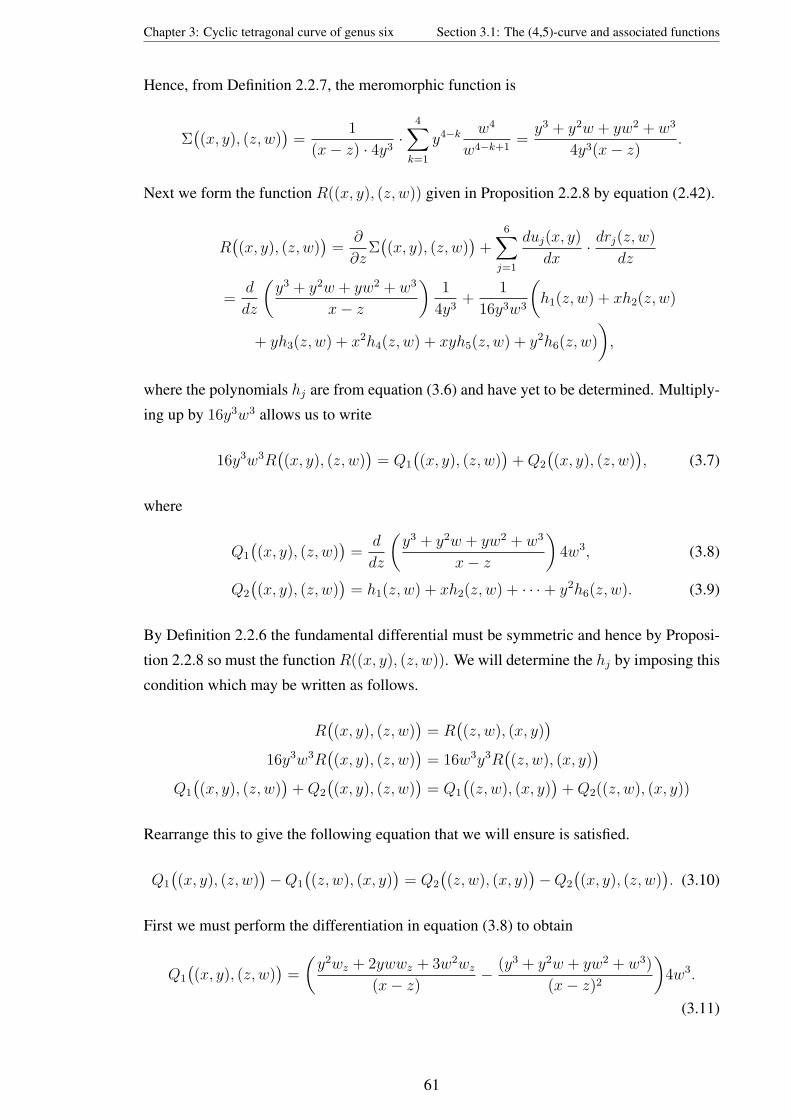
Chapter 3: Cyclic tetragonal curve of genus six Section 3.1: The (4,5)-curve and associated functions
Hence, from Definition 2.2.7, the meromorphic function is
Σ((x, y), (z, w)
)=
1
(x− z) · 4y3·
4∑k=1
y4−k w4
w4−k+1=y3 + y2w + yw2 + w3
4y3(x− z).
Next we form the function R((x, y), (z, w)) given in Proposition 2.2.8 by equation (2.42).
R((x, y), (z, w)
)=
∂
∂zΣ((x, y), (z, w)
)+
6∑j=1
duj(x, y)
dx· drj(z, w)
dz
=d
dz
(y3 + y2w + yw2 + w3
x− z
)1
4y3+
1
16y3w3
(h1(z, w) + xh2(z, w)
+ yh3(z, w) + x2h4(z, w) + xyh5(z, w) + y2h6(z, w)
),
where the polynomials hj are from equation (3.6) and have yet to be determined. Multiply-
ing up by 16y3w3 allows us to write
16y3w3R((x, y), (z, w)
)= Q1
((x, y), (z, w)
)+Q2
((x, y), (z, w)
), (3.7)
where
Q1
((x, y), (z, w)
)=
d
dz
(y3 + y2w + yw2 + w3
x− z
)4w3, (3.8)
Q2
((x, y), (z, w)
)= h1(z, w) + xh2(z, w) + · · ·+ y2h6(z, w). (3.9)
By Definition 2.2.6 the fundamental differential must be symmetric and hence by Proposi-
tion 2.2.8 so must the function R((x, y), (z, w)). We will determine the hj by imposing this
condition which may be written as follows.
R((x, y), (z, w)
)= R
((z, w), (x, y)
)16y3w3R
((x, y), (z, w)
)= 16w3y3R
((z, w), (x, y)
)Q1
((x, y), (z, w)
)+Q2
((x, y), (z, w)
)= Q1
((z, w), (x, y)
)+Q2((z, w), (x, y))
Rearrange this to give the following equation that we will ensure is satisfied.
Q1
((x, y), (z, w)
)−Q1
((z, w), (x, y)
)= Q2
((z, w), (x, y)
)−Q2
((x, y), (z, w)
). (3.10)
First we must perform the differentiation in equation (3.8) to obtain
Q1
((x, y), (z, w)
)=
(y2wz + 2ywwz + 3w2wz
(x− z)− (y3 + y2w + yw2 + w3)
(x− z)2
)4w3.
(3.11)
61

Chapter 3: Cyclic tetragonal curve of genus six Section 3.1: The (4,5)-curve and associated functions
We simplify this by using the curve equation,
w4 = z5 + +λ4z4 + λ3z
3 + λ2z2 + λ1z + λ0. (3.12)
Differentiating the curve equation with respect to z gives
4w3wz = 5z4 + 4λ4z3 + 3λ3z
2 + 2λ2z + λ1
wz =5z4 + 4λ4z
3 + 3λ3z2 + 2λ2z + λ1
4w3. (3.13)
Then substituting (3.12) and (3.13) into (3.11) gives
Q1
((x, y), (z, w)
)=
[1
(x− z)2
] [4y3w3 + w2
(λ1z + 9λ3z
2x− 8λ4z4 − 2λ2z
2
+ 3λ1x+ 12λ4z3x− 5λ3z
3 + 4λ0 − 11z5 + 15z4x+ 6λ2zx)
+ w(2yλ1z
+ 4yλ2zx+ 8yλ4z3x+ 2yλ1x− 4yλ4z
4 − 2yλ3z3 + 4yλ0 − 6yz5 + 6yλ3z
2x
+ 10yz4x)
+ 2y2λ2z2 + 2y2λ2zx+ 5y2z4x+ 3y2λ1z + y2λ3z
3 + 4y2λ0
− y2z5 + y2λ1x+ 4y2λ4z3x+ 3y2λ3z
2x]. (3.14)
We can now form the left hand side of equation (3.10) by reversing the roles in equation
(3.14) and subtracting the new equation from the old. After considerable canceling of terms
this leaves us with
LHS(3.10) = wy(2xλ3 − 2zλ3 − 2z2x+ 2x2z − 4z2λ4 + 4x2λ4 − 6z3 + 6x3
)+ y2
(2λ2 + 8x2λ4 + 7x2z + 3z2x+ 11x3 + 5xλ3 + zλ3 + 4xzλ4 − z3
)− w2
(2λ2 + 8z2λ4 + 7z2x+ 3x2z + 11z3 + 5zλ3 + xλ3 + 4xzλ4 − x3
).
We have been able to collect this into three parts; the terms which contain w2, the terms
which contain y2 and the terms which contain wy. The right hand side of equation (3.10) is
simply
RHS(3.10) = h1(x, y) + zh2(x, y) + wh3(x, y) + z2h4(x, y) + zwh5(x, y) + w2h6(x, y)
− h1(z, w)− xh2(z, w)− yh3(z, w)− x2h4(z, w)− xyh5(z, w)− y2h6(z, w).
We can now assign values to the hj so that equation (3.10) holds. First set h1(x, y) to be
the terms in LHS(3.10) that do not contain z or w.
h1(x, y) = y2(11x3 + 5xλ3 + 8x2λ4 + 2λ2
).
These must all come from the section of terms that contain y2. Similarly, the terms on the
left hand side of equation (3.10) that do not contain w but do contain a single power of z
62

Chapter 3: Cyclic tetragonal curve of genus six Section 3.1: The (4,5)-curve and associated functions
must also come from the y2 section. We set these to be zh2(x, y).
zh2(x, y) = y2(zλ3 + 7x2z + 4xzλ4
)=⇒ h2(x, y) = y2
(λ3 + 7x2 + 4xλ4
).
Next set z2h4(x, y) to be those terms on the left hand side of equation (3.10) that do not
contain w but do contain a single power of z2.
z2h4(x, y) = y2(3z2x
), =⇒ h4(x, y) = 3y2x.
We have now determined values for three of the six hj . Substitute these values into equation
(3.10) and cancel terms to obtain
wy(2xλ3 − 2zλ3 − 2z2x+ 2x2z − 4z2λ4 + 4x2λ4 − 6z3 + 6x3
)+ w2x3 − y2z3
= wh3(x, y) + zwh5(x, y) + w2h6(x, y)− yh3(z, w)− xyh5(z, w)− y2h6(z, w).
(3.15)
Now, the only term on the left of equation (3.15) containing w2 is w2x3 so set
h6(x, y) = x3.
Then set those terms on the left hand side of equation (3.15) with a single power of w and
no z to be wh3(x, y).
wh3(x, y) = wy(2xλ3 + 4x2λ4 + 6x3
)=⇒ h3(x, y) = 2xy
(λ3 + 2xλ4 + 3x2
).
Substituting the expressions for h3 and h6 into equation (3.15) leaves us with
wy(− 2z2x+ 2x2z
)= zwh5(x, y)− xyh5(z, w).
Hence we must have
zwh5(x, y) = wy(2x2z), =⇒ h5(x, y) = 2x2y.
Note that this set of polynomials is not unique. If we had proceeded in a different order then
some of the terms may have been put into different polynomials hj . However, this would
make no difference to the end results.
Substituting the expressions for the hj into equation (3.8) gives
Q2
((x, y), (z, w)
)=(11w2z3 + 5w2zλ3 + 8w2λ4z
2 + 2w2λ2
)+ 3w2x2z + y2z3
+ 2wyz2x+ x(w2λ3 + 7w2z2 + 4zw2λ4
)+(6wz3 + 4z2wλ4 + 2zwλ3
)y. (3.16)
Then substituting equations (3.14) and (3.16) into equation (3.7) gives an explicit equation
63

Chapter 3: Cyclic tetragonal curve of genus six Section 3.1: The (4,5)-curve and associated functions
for R((x, y), (z, w)).
R((x, y), (z, w)
)=
[1
16w3y3(x− z)2
] [3w2x4z + 3λ1w
2x+ λ3w2x3 + 4y2λ0
+ 3y2z4x+ w2λ1z + 4wyλ2zx+ 2wyλ3z2x+ 4y3w3 + w2x3z2 + y2z3x2
+ 2y2λ2zx+ 3y2λ3z2x+ 4y2λ4z
3x+ y2λ1x+ 3y2λ1z + 2y2λ2z2 + y2λ3z
3
+ 4wyλ0 + 2w2λ2x2 + 4z2wyλ4x
2 + 2zwyλ3x2 + 2wyλ1z + 2wyλ1x
+ 2z3wyx2 + 2wyz2x3 + 4w2λ0 + 2w2λ2xz + 4w2λ4x3z + 3w2λ3x
2z
].
We can substitute this into equation (2.41) to give an explicit realisation of the fundamental
differential presented in the summary below. In the extra Appendix of files there is a Maple
worksheet in which these calculations were performed.
Summary
The fundamental differential of the second kind associated to the (4,5)-curve is given by
Ω((x, y), (z, w)
)=F((x, y), (z, w)
)dxdz
16(x− z)2y3w3, (3.17)
where F is the following symmetric polynomial
F((x, y), (z, w)
)= 4y3w3 +
(3xz4 + z3λ3 + z3x2 + 2λ2z
2 + 3xλ3z2
+ 4z3xλ4 + 4λ0 + λ1x+ 2λ2xz + 3λ1z)y2 +
(2λ1z + 4λ2xz + 4λ0 + 2λ1x
+ 4x2λ4z2 + 2λ3x
2z + 2x3z2 + 2z3x2 + 2xλ3z2)wy +
(λ3x
3 + 4λ0
+ 3λ1x+ 2λ2x2 + λ1z + x3z2 + 3x4z + 2λ2xz + 3λ3x
2z + 4λ4x3z)w2. (3.18)
In obtaining this realisation, the following explicit basis for the differentials of the second
kind associated to the cyclic (4,5)-curve was derived.
dr = (dr1, . . . , dr6), where drj(x, y) =hj(x, y)
4y3dx, (3.19)
with
h1(x, y) = y2(11x3 + 5xλ3 + 8x2λ4 + 2λ2
)h4(x, y) = 3y2x
h2(x, y) = y2(λ3 + 7x2 + 4xλ4
)h5(x, y) = 2x2y
h3(x, y) = 2xy(λ3 + 2xλ4 + 3x2
)h6(x, y) = x3.
3.1.2 Abelian functions associated with the (4,5)-curve
We can now proceed to define Abelian functions as in the general case. Start by choosing
an appropriate basis of cycles upon the surface defined by C, (ensuring condition (2.45) on
the intersection numbers is satisfied.) We label these αi, βj, for 1 ≤ i, j ≤ 6 and define the
64

Chapter 3: Cyclic tetragonal curve of genus six Section 3.1: The (4,5)-curve and associated functions
period matrices by integrating (3.4) and (3.19) around these cycles.
ω′ =(∮
αkdu`
)k,`=1,...,6
ω′′ =(∮
βkdu`
)k,`=1,...,6
η′ =(∮
αkdr`
)k,`=1,...,6
η′′ =(∮
βkdr`
)k,`=1,...,6
.
These can be combined into the matrixM which satisfies the generalised Legendre equation
given earlier in (2.53).
M =
(ω′ ω′′
η′ η′′
).
Let Λ denote the lattice generated by the first pair of period matrices, (Definition 2.2.10),
and define an Abelian function associated to C as a meromorphic function that is periodic
over this lattice, (Definition 2.2.11).
By Definition 2.2.12 the Jacobian of C is J = C6/Λ and by Definition 2.2.13 the Abel
map associated to the (4, 5)-curve is defined by
A : Symk(C)→ J
(P1, . . . , Pk) 7→(∫ P1
∞du+ · · ·+
∫ Pk
∞du
)(mod Λ), (3.20)
where the Pi are points upon C. Finally by Definition 2.2.14 the strata of the Jacobian are
the images of the Abel map. When k = 1 the Abel map gives an embedding of the curve C
upon which we define ξ as the local parameter at the origin, A1(∞).
ξ = x−14 . (3.21)
The local parameter at infinity
Many calculations are easily performed at ∞ with the aid of the local parameter ξ. We
derive here series expansion in ξ for the main variables. First, note that in terms of ξ,
x =1
ξ4,
dx
dξ= − 4
ξ5, (3.22)
and
y =(x5 + λ4x
4 + · · ·+ λ1x+ λ0
) 14 =
(ξ−20 + λ4ξ
−16 + · · ·+ λ1ξ−4 + λ0
) 14
=1
ξ5+
(λ4
4
)1
ξ+
(λ3
4− 3λ2
4
32
)ξ3 +
(λ2
4− 3λ4λ3
16+
7λ34
128
)ξ7
+
(λ1
4− 3λ4λ3
16− 3λ2
3
32+
21λ24λ3
128− 77λ4
4
2048
)ξ11 +O(ξ15). (3.23)
65

Chapter 3: Cyclic tetragonal curve of genus six Section 3.1: The (4,5)-curve and associated functions
(See Appendix C.1 for a longer expansion.) Using these substitutions we can calculate se-
ries expansions for the six holomorphic differentials in the basis du given by equation (3.4).
du1 = [−ξ10 +O(ξ14)]dξ du4 = [−ξ2 +O(ξ6)]dξ
du2 = [−ξ6 +O(ξ10)]dξ du5 = [−ξ1 +O(ξ5)]dξ
du3 = [−ξ5 +O(ξ9)]dξ du6 = [−1 +O(ξ4)]dξ.
(3.24)
Integrating these gives us a set of series expansions for the variables u.
u1 = − 111ξ11 +O(ξ15) u3 = −1
6ξ6 +O(ξ10) u5 = −1
2ξ2 +O(ξ6)
u2 = −17ξ7 +O(ξ11) u4 = −1
3ξ3 +O(ξ7) u6 = −ξ +O(ξ5).
(3.25)
Note that the higher order terms in (3.24) and (3.25) will all depend on the curve parameters
λ0, . . . , λ4. (See Appendix C.1 for larger expansions).
Abelian functions
Define the Kleinian σ-function associated to the (4, 5)-curve as in Definition 2.2.15 and
note that it is a function of g = 6 variables.
σ = σ(u) = σ(u1, u2, u3, u4, u5, u6).
Define the 2-index ℘-functions associated to the (4, 5)-curve as in Definition 2.2.24.
℘i,j(u) = − ∂
∂ui
∂
∂ujlog[σ(u)
], i ≤ j ∈ 1, . . . , 6.
There will be 21 of the 2-index ℘-functions,
℘ij = ℘11, ℘12, ℘13, ℘14, ℘15, ℘16, ℘22, ℘23, ℘24, ℘25, ℘26,
℘33, ℘34, ℘35, ℘36, ℘44, ℘45, ℘46, ℘55, ℘56, ℘66.
Similarly we can define the n-index ℘-functions as in Definition 2.2.27.
℘i1,i2,...,in(u) = − ∂
∂ui1
∂
∂ui2. . .
∂
∂uinlog[σ(u)
], i1 ≤ · · · ≤ in ∈ 1, . . . , 6.
There will be 56 of the 3-index ℘-functions and 126 of the 4-index ℘-functions.
In Lemma 2.2.28 the n-index ℘-functions were shown to have poles of order n when
σ(u) = 0. By Lemma 2.2.19 this occurs when u ∈ Θ[5]. Any Abelian function that is
holomorphic must be constant (by a generalisation of Liouville’s theorem) and it is not
possible for an Abelian function to have simple poles. Hence those Abelian functions with
poles of order two have the simplest pole structure possible and are sometimes referred to
as fundamental Abelian functions. (Note that the Weierstrass ℘-function is in this category.)
66

Chapter 3: Cyclic tetragonal curve of genus six Section 3.1: The (4,5)-curve and associated functions
3.1.3 The Q-functions
We find in Section 3.5 that the 2-index ℘-functions are not sufficient to construct a basis for
the fundamental Abelian functions associated to the (4,5)-curve. We overcome this problem
by considering another class of Abelian functions, alongside the ℘-functions. These can
also be defined using the Kleinian σ-functions and the following operator.
Definition 3.1.1. Define the operator ∆i as below. This is now known as Hirota’s bilinearoperator, although it was used much earlier by Baker in [10].
∆i =∂
∂ui− ∂
∂vi.
We now check that an alternative, equivalent definition of the 2-index Kleinian ℘-
functions is given by
℘ij(u) = − 1
2σ(u)2∆i∆jσ(u)σ(v)
∣∣∣v=u
i ≤ j ∈ 1, . . . , 6. (3.26)
Applying the operator as defined above we see that
∆j
[σ(u)σ(v)
]=
∂
∂uj[σ(u)σ(v)]− ∂
∂vj[σ(u)σ(v)] = σ(v)σj(u)− σ(u)σj(v),
∆i∆j
[σ(u)σ(v)
]= σ(v)σij(u)− σi(u)σj(v)− σi(v)σj(u) + σ(u)σij(v).
Hence equation (3.26) may be evaluated as follows:
℘ij(u) = − 1
2σ(u)2∆i∆jσ(u)σ(v)
∣∣∣v=u
= − 1
2σ(u)2
[σ(v)σij(u)− σi(u)σj(v)− σi(v)σj(u) + σ(u)σij(v)
]∣∣∣v=u
= − 1
2σ(u)2
[2σ(u)σij(u)− 2σi(u)σj(u)
]=σi(u)σj(u)− σ(u)σij(u)
σ(u)2
This is the same ratio of σ-derivatives as we obtained in equation (2.61) from the original
definition of ℘ij(u). Hence the two definitions are indeed equivalent. We now extend this
approach to define a new class of functions.
Definition 3.1.2. Define then-indexQ-functions, for n even, associated to an (n, s)-curve
with genus g by
Qi1,i2,...,in(u) =(−1)
2σ(u)2∆i1∆i2 . . .∆inσ(u)σ(v)
∣∣∣v=u
(3.27)
where i1 ≤ · · · ≤ in ∈ 1, . . . , g.
Note that these functions are all independent of the constant c used in the definition of
the σ-function. (See Appendix B for the proof.)
67

Chapter 3: Cyclic tetragonal curve of genus six Section 3.1: The (4,5)-curve and associated functions
Lemma 3.1.3. The n-index Q-functions are meromorphic functions with poles of order two
when σ(u) = 0.
Proof. Applying the Hirota operator on σ(u)σ(v) repeatedly yields a polynomial of σ-
derivatives, all of which are entire functions. Hence a Q-function is an entire function
divided by σ(u)2 and so will have poles of order two only when σ(u) = 0.
These functions are a generalisation of theQ-functions used by Baker in his work on the
(2,5)-case. The 4-index Q-functions have been considered before when similar problems
occurred in research on the trigonal curves. In these papers the 4-index Q-functions are
just defined as Q-functions and are sufficient to complete the basis of fundamental Abelian
functions. However, in the (4, 5)-case we will find that it is necessary to use a 6-index Q-
function and in higher genus cases it is inevitable that even higher index Q-functions would
be necessary. Hence we have given this general definition.
Remark 3.1.4.
(i) From now on we may write just refer to the Q-functions, specifying if we are working
with functions of a particular index.
(ii) The subscripts of the ℘-functions denote differentiation
∂
∂uin+1
℘i1,i2,...,in = ℘i1,i2,...,in,in+1 ,
but this is not the case for the Q-functions. Here the indices refer to which Hirota
operators were used.
Lemma 3.1.5. If Definition 3.1.2 were applied with n odd then the resulting function is
identically zero.
Proof. Let f(u,v) be a symmetric function.
f(u,v) = f(v,u).
Consider the Hirota operator applied to such a function.
∆if(u,v) =∂
∂uif(u,v)− ∂
∂vif(u,v) =
∂
∂uif(u,v)− ∂
∂vif(v,u).
Let f be the derivative of f with respect to the ith component of its first variable. Then
∆if(u,v) = f(u,v)− f(v,u). (3.28)
Now consider the Hirota operator applied a second time.
∆j∆if(u,v) =∂
∂ujf(u,v)− ∂
∂ujf(v,u)− ∂
∂vjf(u,v) +
∂
∂vjf(v,u).
68

Chapter 3: Cyclic tetragonal curve of genus six Section 3.1: The (4,5)-curve and associated functions
Let f1 and f2 be the derivative of f with respect to the jth component of its first variable
and second variables respectively.
∆j∆if(u,v) = f1(u,v)− f2(v,u)− f2(u,v) + f1(v,u). (3.29)
Note that the right hand side is symmetric.
∆j∆if(v,u) = f1(v,u)− f2(u,v)− f2(v,u) + f1(u,v) = ∆j∆if(u,v). (3.30)
Now consider the effect on equation (3.28) of setting v = u.
∆if(u,v)∣∣∣v=u
= f(u,u)− f(u,u) = 0. (3.31)
An n-index Q-function is constructed by applying n Hirota derivatives to σ(u)σ(v) and
then setting v = u. Since σ(u)σ(v) is symmetric, we can conclude that a 1-index Q-
function must be zero by equation (3.29).
By equation (3.30), the application of two Hirota operators on σ(u)σ(v) will generate a
symmetric function. Similarly any even application of Hirota operators on σ(u)σ(v) would
also generate a symmetric function. Finally, we can apply equation (3.31) to conclude that
any n-index Q-function with n odd must be zero.
In [30] it was shown that the 4-indexQ-functions could be expressed using the Kleinian
℘-functions as follows.
Qijk` = ℘ijk` − 2℘ij℘k` − 2℘ik℘j` − 2℘i`℘jk. (3.32)
This specialises to
Qijkk = ℘ijkk − 2℘ij℘kk − 4℘ik℘jk, Qiijj = ℘iijj − 2℘ii℘jj − 4℘2ij,
Qijjj = ℘ijjj − 6℘ij℘jj, Qiiii = ℘iiii − 6℘2ii.
A similar result is presented here for the 6-index Q-functions.
Proposition 3.1.6. The 6-index Q-functions may be written as
Qijklmn = ℘ijklmn − 2[(℘ij℘klmn + ℘ik℘jlmn + ℘il℘jkmn + ℘im℘jkln + ℘in℘jklm
)+(℘jk℘ilmn + ℘jl℘ikmn + ℘jm℘ikln + ℘jn℘iklm
)+(℘kl℘ijmn + ℘km℘ijln + ℘kn℘ijlm
)+(℘lm℘ijkn + ℘ln℘ijkm
)+ ℘mn℘ijkl
]+ 4[(℘ij℘kl℘mn + ℘ij℘km℘ln + ℘ij℘kn℘lm
)+(℘ik℘jl℘mn + ℘ik℘jm℘ln + ℘ik℘jn℘lm
)+(℘il℘jk℘mn + ℘il℘jm℘kn + ℘il℘jn℘km
)+(℘im℘jk℘ln + ℘im℘jl℘kn + ℘im℘jn℘kl
)+(℘in℘jk℘lm + ℘in℘jl℘km + ℘in℘jm℘kl
)].
69

Chapter 3: Cyclic tetragonal curve of genus six Section 3.1: The (4,5)-curve and associated functions
Proof. Apply Definitions 2.2.27 and 3.1.2 to reduce the equation to a sum of rational func-
tions involving σ-derivatives. We find that they all cancel (Maple is useful here). The
actual structure of the sum was prompted by considering the existing result for the 4-index
Q-functions.
Corollary 3.1.7. The 4-index and 6-index Q-functions are even Abelian functions.
Proof. Equations (3.32) and Proposition 3.1.6 demonstrate that these functions may be
expressed as a sum of even Abelian functions, and hence they are themselves even Abelian
functions.
The proof that all n-index Q-functions are even and Abelian will involve a lengthly in-
duction. This document uses only 4 and 6-index Q-function so Corollary 3.1.7 is sufficient.
Note that Proposition 3.1.6 specialises to the following set of formulae.
Qijklmm = ℘ijklmm − 2℘ij℘klmm − 2℘ik℘jlmm − 2℘il℘jkmm − 4℘im℘jklm − 2℘jk℘ilmm
− 2℘jl℘ikmm − 4℘jm℘iklm − 2℘kl℘ijmm − 4℘km℘ijlm − 4℘lm℘ijkm
− 2℘mm℘ijkl + 8℘ik℘jm℘lm + 8℘im℘jl℘km + 8℘ij℘km℘lm + 8℘il℘jm℘km
+ 4℘ij℘kl℘mm + 4℘ik℘jl℘mm + 4℘il℘jk℘mm + 8℘im℘jm℘kl + 8℘im℘jk℘lm
Qijklll = ℘ijklll − 2℘ij℘klll − 2℘ik℘jlll − 6℘il℘jkll − 2℘jk℘illl − 6℘jl℘ikll − 6℘kl℘ijll
− 6℘ll℘ijkl + 12℘ij℘kn℘ll + 12℘ik℘jl℘ll + 12℘il℘jk℘ll + 24℘il℘jl℘kl
Qijkkll = ℘ijkkll + 16℘ik℘jl℘kl + 8℘il℘jl℘kk − 4℘jl℘ikkl + 16℘il℘jk℘kl + 8℘ij℘2kl
− 2℘ij℘kkll − 4℘jk℘ikll + 4℘ij℘kk℘ll + 8℘ik℘jk℘ll − 2℘kk℘ijll − 4℘ik℘jkll
− 8℘kl℘ijkl − 2℘ll℘ijkk − 4℘il℘jkkl
Qijkkkk = ℘ijkkkk − 2℘ij℘kkkk − 8℘ik℘jkkk − 8℘jk℘ikkk + 48℘ik℘jk℘kk
+ 12℘ij℘2kk − 12℘kk℘ijkk
Qijjkkk = ℘ijjkkk + 12℘ik℘jj℘kk + 24℘ik℘2jk + 24℘ij℘jk℘kk − 4℘ij℘jkkk − 6℘kk℘ijjk
− 6℘ik℘jjkk − 2℘jj℘ikkk − 12℘jk℘ijkk
Qiijjkk = ℘iijjkk + 4℘ii℘jj℘kk + 32℘ik℘ij℘jk + 8℘2ij℘kk − 2℘ii℘jjkk − 2℘jj℘iikk
+ 8℘2ik℘jj + 8℘ii℘
2jk − 8℘jk℘iijk − 2℘kk℘iijj − 8℘ij℘ijkk − 8℘ik℘ijjk
Qijjjjj = ℘ijjjjj − 10℘ij℘jjjj + 60℘ij℘2jj − 20℘jj℘ijjj
Qiijjjj = ℘iijjjj − 2℘ii℘jjjj − 12℘jj℘iijj − 16℘ij℘ijjj + 48℘2ij℘jj + 12℘ii℘
2jj
Qiiijjj = ℘iiijjj − 6℘jj℘iiij + 36℘ij℘ii℘jj − 6℘ii℘ijjj − 18℘ij℘iijj + 24℘3ij
Qiiiiii = ℘iiiiii − 30℘ii℘iiii + 60℘3ii
70

Chapter 3: Cyclic tetragonal curve of genus six Section 3.2: Expanding the Kleinian formula
3.2 Expanding the Kleinian formula
This section is based upon the following Theorem, originally by Klein and given for a gen-
eral (n, s)-curve as Theorem 3.4 in [35]. The result is derived from the Riemann Vanishing
Theorem for the θ-function, in which the σ-function and hence the ℘-function can be ex-
pressed. In this section we will use the theorem applied to the (4,5)-case to solve the Jacobi
Inversion Problem, as well as generate relations between the ℘-functions.
Theorem 3.2.1. Let P1, . . . , P6 be an arbitrary set of distinct points on C, and (z, w)
any point of this set. Then for an arbitrary point (x, y) and the base point∞ on C we have
6∑i,j=1
℘ij
(∫ (x,y)
∞du−
6∑k=1
∫ Pk
∞du
)gi(x, y)gj(z, w) =
F((x, y), (z, w)
)(x− z)2
.
(3.33)
Here gi is the numerator of dui from the standard basis of holomorphic differentials and
F ((x, y), (z, w)) the symmetric function that appeared in Klein’s realisation of the funda-
mental differential. These have already been derived for the cyclic (4,5)-case with the gipresented in equation (3.4) the symmetric function given by equation (3.18).
Equation (3.33) is often referred to as the Kleinian formula. We now describe how
equations between the ℘-functions can be derived from this theorem. We will describe
the steps taken, although it is recommended the calculations be performed in a computer
algebra package such as Maple. Define
u =
∫ (x,y)
∞du−
6∑k=1
∫ Pk
∞du
and consider the effect on u as the point (x, y) tends to infinity. We may describe this by
writing u = u + uξ where u ∈ C6 and u is a vector containing the series expansions in ξ
of the variables. (These expansions were derived in equation (3.25) with longer expansions
given in Appendix C.1.)
Taking the Taylor series series expansion in ξ we see that
℘ij(u) =[℘ij − ℘6ijξ +
(12℘66ij − 1
2℘5ij
)ξ2 −
(16℘666ij + 1
3℘4ij − 1
2℘56ij
)ξ3
+(
124℘6666ij + 1
8℘55ij − 1
4℘566ij + 1
3℘46ij
)ξ4 −
(1
120℘66666ij − 1
20℘6ijλ4
+ 18℘556ij − 1
12℘5666ij − 1
6℘45ij + 1
6℘466ij
)ξ5 −
(1
720℘666666ij + 1
48℘555ij
+ 118℘44ij + 1
12℘5ijλ4 − 1
20℘66ijλ4 − 1
6℘456ij − 1
48℘56666ij + 1
18℘4666ij − 1
6℘3ij
+ 116℘5566ij
)ξ6 −
(1
5040℘6666666ij + 1
7℘2ij − 3
28℘4ijλ4 − 1
40℘666ijλ4 + 1
18℘446ij
+ 13120λ4℘56ij + 1
48℘55666ij + 1
72℘46666ij − 1
6℘36ij − 1
240℘566666ij − 1
12℘4566ij + . . .
71

Chapter 3: Cyclic tetragonal curve of genus six Section 3.2: Expanding the Kleinian formula
· · ·+ 124℘455ij − 1
48℘5556ij
)ξ7 +
(1
40320℘66666666ij + 1
192℘556666ij + 1
384℘5555ij
+ 112℘35ij + 1
7℘26ij − 1
96℘55566ij + 1
360℘466666ij − 1
120℘6666ijλ4 + 1
15℘566ijλ4
− 136℘445ij − 13
105℘46ijλ4 − 1
24℘55ijλ4 − 1
1440℘5666666ij − 1
12℘366ij − 1
36℘45666ij
+ 136℘4466ij + 1
24℘4556ij
)ξ8 +
(− 1
362880℘666666666ij − 1
384℘55556ij − 1
12℘356ij
+ 110080
℘56666666ij + 1144℘456666ij − 1
48℘45566ij − 1
108℘44666ij + 1
144℘4555ij
+ 136℘6ijλ3 − 5
288℘6ijλ4
2 + 118℘34ij + 1
288℘555666ij − 1
2160℘4666666ij + 1
36℘3666ij
− 1960℘5566666ij + 1
36℘4456ij + 1
14℘25ij − 1
14℘266ij − 1
162℘444ij − 41
504℘45ijλ4
+ 59840λ4℘466ij + 23
480℘556ijλ4 − 19
720λ4℘5666ij + 1
480℘66666ijλ4
)ξ9 +O(ξ10)
](u).
(Note that the final (u) is notation to indicate that the right hand side is a function of
u ∈ C6). Now let us construct a series expansion in ξ for equation (3.33) as (x, y) tends to
infinity.
Start by forming the sum on the left hand side using the expansion above and the poly-
nomials gi in equation (3.4). The sum runs for all i, j ∈ (1, . . . , 6). Multiply this by (x−z)2
and subtract the polynomial F given in equation (3.18). Substitute for the variables (x, y)
using their expansions in ξ. Then multiply out to form a final series expansion in ξ that
must equal zero.
The coefficients of the ξ will be polynomials in ℘-functions and the variables (z, w). It
follows that each coefficient with respect to ξ must be zero for any u and some (z, w) on C.
This gives us a potentially infinite sequence of equations, starting with the five equations
given below.
0 = ρ1 = −z3 + ℘46z2 + (℘56w + ℘26) z + ℘66w
2 + ℘36w + ℘16 (3.34)
0 = ρ2 = (℘45 − ℘466 − 2w) z2 + ((℘55 − ℘566)w + ℘25 − ℘266) z
+ (℘56 − ℘666)w2 + (℘35 − ℘366)w + ℘15 − ℘166 (3.35)
0 = ρ3 =(℘44 − 3
2℘456 + 1
2℘4666
)z2 +
(− 3w2
(℘45 − 3
2℘556 + 1
2℘5666
)w − 3
2℘256
+ ℘24 + 12℘2666
)z +
(12℘6666 − 3
2℘566 + ℘46
)w2 +
(12℘3666 + ℘34 − 3
2℘356
)w
+ ℘14 + 12℘1666 − 3
2℘156
0 = ρ4 =(℘4566 − 4
3℘446 − 1
6℘46666 − 1
2℘455
)z2 +
((℘5566 − 4
3℘456 − 1
6℘56666 − 1
2℘555
)w
− 43℘246 − 1
2℘255 + ℘2566 − 1
6℘26666
)z − 4w3 +
(℘5666 − 1
2℘556 − 1
6℘66666 − 4
3℘466
)w2
+(− 1
6℘36666 + ℘3566 − 4
3℘346 − 1
2℘355
)w − 1
6℘16666 + ℘1566 − 4
3℘146 − 1
2℘155
0 = ρ5 = −3z4 −(2℘46 + 9
2λ4
)z3 +
(58℘4556 − 5
6℘445 − 5
12℘45666 − 2℘56w − 2℘26 − 3λ3
+ 56℘4466 + 1
2℘46λ4 + 1
24℘466666
)z2 +
(− 2℘66w
2 +(
124℘566666 − 5
6℘455 + 5
6℘4566
− 512℘55666 + 1
2℘56λ4 − 2℘36 + 5
8℘5556
)w − 5
12℘25666 − 5
6℘245 − 2λ2 + 5
6℘2466 + . . .
72

Chapter 3: Cyclic tetragonal curve of genus six Section 3.2: Expanding the Kleinian formula
· · ·+ 58℘2556 + 1
24℘266666 − 2℘16 + 1
2℘26λ4
)z +
(12℘66λ4 − 5
12℘56666 + 1
24℘666666
− 56℘456 + 5
6℘4666 + 5
8℘5566
)w2 +
(124℘366666 + 5
6℘3466 + 5
8℘3556 + 1
2℘36λ4 − 5
6℘345
− 512℘35666
)w + 5
8℘1556 − 5
12℘15666 + 1
24℘166666 − λ1 + 5
6℘1466 − 5
6℘145 + 1
2℘16λ4
These equations all contain ℘-functions and the variables z, w. They are valid for any
u ∈ C6, with (z, w) one of the points on C that are used in equation (3.5) to represent u.
We have labeled the polynomials ρi for later use. They are presented in ascending order
(as the coefficients of ξ). The polynomials have been calculated explicitly up to ρ14 (using
Maple). They get increasingly larger in size and can be found in the extra Appendix of files
or online at [38]. The Maple worksheet in which they are derived may also be found in the
extra Appendix of files.
3.2.1 Generating relations between the ℘-functions
We now describe how these equations may be manipulated in order to generate relations be-
tween the ℘-functions. We achieve this by eliminating variables between pairs of equations
using the method of resultants. Appendix A.6 gives a definition of the resultant, details on
its construction and a simple example to demonstrate its use. For more information we re-
fer the reader to [43] Chapter 12. The calculations were performed in the computer algebra
package Maple using the inbuilt resultant function.
The first step is to take pairs of the equations derived above and take resultants to elim-
inate the variable w. (Note that equivalently we could have started by eliminating the
variable z.) Denote the resultant of polynomials ρi and ρj by ρi,j . Since ρi and ρj were
equal to zero, so must the resultant that is obtained.
ρi,j = Res(ρi, ρj) = 0.
This gives us a set of new equations in z and the ℘-functions. These equations are quite
large and so are not printed here. Instead we present Table 3.1 detailing the number of terms
they contain once expanded and the degree in z.
Note that when examining combinations that involved the higher ρi a polynomial with
degree in z that was less than seven was never found. In general, the higher the ρi involved
in the resultant, the more terms the resultant would have.
The next step is to combine these to find polynomials of degree five in z. By the fol-
lowing theorem such polynomials would be zero. This would allow us to set each of the
coefficients of the polynomial to zero, giving relations between ℘-functions.
73

Chapter 3: Cyclic tetragonal curve of genus six Section 3.2: Expanding the Kleinian formula
Table 3.1: Details on the polynomials ρi,j
resultant # terms degree in zρ1,2 317 7ρ1,3 744 8ρ1,4 1526 9ρ1,5 2080 8ρ2,3 2670 7ρ2,4 9479 8ρ2,5 13943 9ρ3,4 30756 7ρ3,5 31592 10ρ4,5 311250 12
Theorem 3.2.2. Consider an equation in z with coefficients in the ℘-functions evaluated
at an arbitrary point u ∈ Cg. If the equation has degree in z less than g then it must be
identically zero.
Proof. Such a polynomial would have at most g−1 independent roots, but must be satisfied
for g arbitrary variables u ∈ Cg. Hence the polynomial must be identically zero.
So we start by selecting one of the polynomials with degree seven in z and rearrange
it to give an equation for z7. The simplest approach is to use ρ1,2 as it is the smallest such
polynomial. The coefficient of z7 in ρ1,2 is −4℘66 so we may use this equation to write
z7 = − 1
4℘66
(degree six polynomial in z with coefficients in ℘-functions
). (3.36)
Then since ρ1,3 has degree eight in z we can substitute equation (3.36) twice into ρ1,3 to
leave an equation of degree six in z. We label this equation (T1) for future use. (Note that
equation (T1) can be found in the extra Appendix of files or online at [38].)
The next step is to rearrange (T1) to give an equation for z6. Although (T1) is the
simplest such equation, it still has the following non-trivial coefficient of z6.
1
16℘266
(72℘66℘55℘
2666 − 36℘66℘566℘
2666 − 240℘46℘55℘
266 + 48℘46℘566℘
266 − 72℘55℘
266℘566
+ 72℘266℘466℘666 + 24℘66℘46℘
256 + 12℘66℘6666℘
256 − 12℘66℘6666℘
2666 + 72℘66℘36℘666
− 48℘6666℘266℘55 + 96℘2
66℘45℘56 − 36℘66℘55℘256 + 72℘556℘56℘
266 + 64℘46℘6666℘
266
+ 24℘6666℘566℘266 − 24℘5666℘56℘
266 − 96℘66℘
2666℘46 − 144℘2
66℘466℘56 − 72℘266℘45℘666
+ 9℘456 + 9℘4
666 + 72℘66℘56℘46℘666 + 36℘66℘566℘56℘666 − 36℘66℘55℘56℘666
− 72℘66℘36℘56 + 4℘26666℘
266 + 144℘2
66℘35 + 144℘366℘456 − 18℘2
666℘256 − 96℘3
66℘44
− 144℘266℘366 + 108℘2
55℘266 − 48℘3
66℘4666 + 112℘246℘
266 − 144℘26℘
266
). (3.37)
74

Chapter 3: Cyclic tetragonal curve of genus six Section 3.2: Expanding the Kleinian formula
We rearrange (T1) to obtain an equation of the following form for z6.
z6 =1
(3.37)
(degree five polynomial in z with coefficients in ℘-functions
)(3.38)
We may now take any of the other ρi,j and repeatedly substitute for z7 and z6 using equa-
tions (3.36) and (3.38) until we have a polynomial of degree five in z. By Theorem 3.2.2
the coefficients with respect to z of such an equation must be zero. Further, since they are
zero we can take the numerator of the coefficients leaving us with six polynomial equations
between the ℘-functions from each ρi,j .
There is one further simplification to be made by recalling Lemma 2.2.32 which stated
that all the ℘-functions have definite parity. This means that we separate each of these six
relations into their odd and even parts, each of which must independently be zero. We will
denote the polynomial equations between ℘-functions that we generate using this method
as follows.
Definition 3.2.3. Reduce equation ρi,j to degree five in z using equations (3.36) and (3.38).
Then define
K(ρi,j, n,±)
to be the relation achieved by selecting the coefficient with respect to zn, taking the numer-
ator and selecting either the even or odd parts as indicated by + or − respectively.
The simplest of these relations came from the reductions of ρ2,3 and ρ1,5, however these
relations are still very long and complex. We do not print them here but we do present Table
3.2 which indicates the number of terms in each.
Table 3.2: The polynomials K(ρi,j, n,±)
equation # terms equation # termsK(ρ2,3, 5,+) 1907 K(ρ1,5, 5,+) 6631K(ρ2,3, 5,−) 1788 K(ρ1,5, 5,−) 6145K(ρ2,3, 4,+) 6595 K(ρ1,5, 4,+) 18062K(ρ2,3, 4,−) 6405 K(ρ1,5, 4,−) 17105K(ρ2,3, 3,+) 13113 K(ρ1,5, 3,+) 28442K(ρ2,3, 3,−) 12835 K(ρ1,5, 3,−) 27226K(ρ2,3, 2,+) 17152 K(ρ1,5, 2,+) 33892K(ρ2,3, 2,−) 16820 K(ρ1,5, 2,−) 32424K(ρ2,3, 1,+) 12387 K(ρ1,5, 1,+) 23614K(ρ2,3, 1,−) 12192 K(ρ1,5, 1,−) 22723K(ρ2,3, 0,+) 5214 K(ρ1,5, 0,+) 10334K(ρ2,3, 0,−) 5070 K(ρ1,5, 0,−) 9765
75
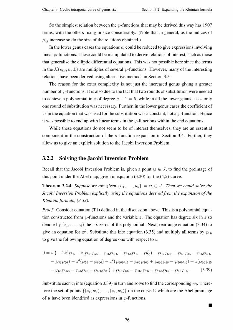
Chapter 3: Cyclic tetragonal curve of genus six Section 3.2: Expanding the Kleinian formula
So the simplest relation between the ℘-functions that may be derived this way has 1907
terms, with the others rising in size considerably. (Note that in general, as the indices of
ρi,j increase so do the size of the relations obtained.)
In the lower genus cases the equations ρi could be reduced to give expressions involving
linear ℘-functions. These could be manipulated to derive relations of interest, such as those
that generalise the elliptic differential equations. This was not possible here since the terms
in the K(ρi,j, n,±) are multiples of several ℘-functions. However, many of the interesting
relations have been derived using alternative methods in Section 3.5.
The reason for the extra complexity is not just the increased genus giving a greater
number of ℘-functions. It is also due to the fact that two rounds of substitution were needed
to achieve a polynomial in z of degree g − 1 = 5, while in all the lower genus cases only
one round of substitution was necessary. Further, in the lower genus cases the coefficient of
zg in the equation that was used for the substitution was a constant, not a ℘-function. Hence
it was possible to end up with linear terms in the ℘-functions within the end equations.
While these equations do not seem to be of interest themselves, they are an essential
component in the construction of the σ-function expansion in Section 3.4. Further, they
allow us to give an explicit solution to the Jacobi Inversion Problem.
3.2.2 Solving the Jacobi Inversion Problem
Recall that the Jacobi Inversion Problem is, given a point u ∈ J , to find the preimage of
this point under the Abel map, given in equation (3.20) for the (4,5)-curve.
Theorem 3.2.4. Suppose we are given u1, . . . , u6 = u ∈ J . Then we could solve the
Jacobi Inversion Problem explicitly using the equations derived from the expansion of the
Kleinian formula, (3.33).
Proof. Consider equation (T1) defined in the discussion above. This is a polynomial equa-
tion constructed from ℘-functions and the variable z. The equation has degree six in z so
denote by (z1, . . . , z6) the six zeros of the polynomial. Next, rearrange equation (3.34) to
give an equation for w2. Substitute this into equation (3.35) and multiply all terms by ℘66
to give the following equation of degree one with respect to w.
0 = w(− 2z2℘66 + z(℘66℘55 − ℘66℘566 + ℘666℘56 − ℘2
56) + ℘36℘666 + ℘66℘35 − ℘66℘366
− ℘36℘56
)+ z3(℘56 − ℘666) + z2(℘66℘45 − ℘66℘466 + ℘666℘46 − ℘56℘46) + z(℘66℘25
− ℘66℘266 − ℘56℘26 + ℘666℘26) + ℘15℘66 − ℘166℘66 + ℘666℘16 − ℘56℘16. (3.39)
Substitute each zi into (equation 3.39) in turn and solve to find the correspondingwi. There-
fore the set of points (z1, w1), . . . , (z6, w6) on the curve C which are the Abel preimage
of u have been identified as expressions in ℘-functions.
76

Chapter 3: Cyclic tetragonal curve of genus six Section 3.3: The Sato weights
3.3 The Sato weights
For any (n, s)-curve we can define a set of weights for all the objects in the theory such
that all equations are homogeneous with respect to these weights. These are known as
Sato weights, although we will often just write weight in this document. The weights have
played an important role in the research on lower genus cases and are used regularly in the
following sections.
In this section we will define and derive the weights associated to the theory of an arbi-
trary (n, s)-curve, giving explicit examples for the cyclic (4,5)-curve. Such a justification
for the weights in the general case has not been presented in the literature, but follows
logically from the general definitions.
We start by defining what we mean by weights.
Definition 3.3.1. Define the weight of an object χ as an integer αχ such that under the
mapping
χ 7→ tαχχ (3.40)
all equations are homogeneous in the variable t. (An equation is homogeneous in t if each
term has the same degree in t.)
From this definition it is clear that the following statements must hold.
weight[a · b
]= weight(a) + weight(b),
weight[ab
]= weight(a)− weight(b),
weight[an]
= n · weight(a)
Given this definition let us derive weights for the variables and parameters of a cyclic
(n, s)-curve such that the curve equation is homogeneous. Start by applying the mapping
(3.40) to the curve equation (2.34).
yn = xs + λs−1xs−1 + · · ·+ λ1x+ λ0(
tαy y)n
=(tαxx
)s+(tαλs−1 λs−1
)(tαxx
)s−1+ · · ·+
(tαλ1 λ1
)(tαxx
)+(tαλ0 λ0
)tnαy yn = tsαxxs + tαλs−1
+(s−1)αxλs−1xs−1 + · · ·+ tαλ1
+αxλ1x+ tαλ0 λ0.
We need this to be homogeneous with respect to t and hence the weights of x and y are
determined up to a constant by
nαy = sαx.
To keep with the convention in the literature we choose these weights so that they are the
77

Chapter 3: Cyclic tetragonal curve of genus six Section 3.3: The Sato weights
largest negative integers satisfying the condition. That is
αx = −n, αy = −s.
The weights of the curve constants are then determined uniquely by ensuring that the other
terms in the equation are also homogeneous. We define this choice as the Sato weights.
Definition 3.3.2. Define the Sato Weights for the curve variables and constants in the
equation of a cyclic (n, s) curve to be
weight[x] = −n, weight[λs−1] = −n,
weight[y] = −s, weight[λs−2] = −2n,
... (3.41)
weight[λ1] = −n(s− 1),
weight[λ0] = −ns.
Define the Sato weight of all other constants to be zero and define the Sato weights of other
objects to be those weights that follow logically from these.
If we had instead used equation (2.32) for a general (n, s) curve then we would have
still had the same condition on the weights of x and y. Making the same choice would lead
us to define the weights of the curve constant µi to be the negative of their subscripts. The
subscripts were chosen in Definition 2.2.1 as a label to satisfy this property.
Example 3.3.3. In the cyclic (4,5)-case we have
+x +y +λ4 +λ3 +λ2 +λ1 +λ0
Weight −4 −5 −4 −8 −12 −16 −20
The next step is to derive the weights of the variables u. They can be determined
uniquely given Definition 3.3.2. Recall the definition of the local parameter for (x, y) as
infinity.
ξ = x−1n .
Applying the mapping (3.40) to this equation,
tαξ ξ =(tαxx
)− 1n = t−
1n
(−n)x = tx.
Hence the Sato weight of the parameter ξ is one for any (n, s)-curve.
Recall that series expansions in ξ can be derived for the basis of holomorphic differen-
tials and hence the variables u.
78

Chapter 3: Cyclic tetragonal curve of genus six Section 3.3: The Sato weights
In the (4,5)-case these were given in equations (3.25) as
u1 = − 111ξ11 +O(ξ15), u3 = −1
6ξ6 +O(ξ10), u5 = −1
2ξ2 +O(ξ6),
u2 = −17ξ7 +O(ξ11), u4 = −1
3ξ3 +O(ξ7), u6 = −ξ +O(ξ5).
Applying the mapping (3.40) and considering the first term of the expansions would lead us
to conclude that the weights of u were given by the leading powers of ξ in the expansions.
Note that the expansions rise in powers of ξ by n = 4, and that the coefficients of the
higher order terms depend on the curve parameters. The weights of the curve parameters
in each coefficient decrease by n = 4 ensuring that the expansion remains homogeneous
and the u have definite Sato weight. (See the larger expansions for the (4,5)-curve given in
Appendix C.1 to check this is the case.)
Theorem 3.3.4. The variables u associated to an (n, s)-curve have definite weight that
may be derived from the series expansions in ξ.
Further these weights may be predicted as follows using the Weierstrass gap sequence
Wn,s = w1, . . . , wg defined in Definition 2.2.3.
weight[u1] = wg = 2g − 1
weight[u2] = wg−1
...
weight[ug−1] = w2 (3.42)
weight[ug] = w1 = 1 (3.43)
Sketch of Proof. Since the weight of ξ is always one it is simple to choose weights of u
to match the first term in the series expansions. The expansions in ξ will always increase
in steps of n, with the coefficients in the curve parameters increasing in weight by n. This
is because the infinite expansions came only from the variable y which was in each differ-
ential of the basis. Hence the variables u associated to an (n, s)-curve always have definite
weight.
The dependency on the Weierstrass gap sequence is due to the fact that the standard
basis of holomorphic differentials that we use was constructed from Wn,s. (See Proposi-
tion 2.2.4).
Example 3.3.5. In the (4,5)-case we assign the following weights to u.
u1 u2 u3 u4 u5 u6
Weight +11 +7 +6 +3 +2 +1
79

Chapter 3: Cyclic tetragonal curve of genus six Section 3.3: The Sato weights
Remark 3.3.6.
(i) The weights of the variables coincide with the order of their zero at∞.
(ii) The weights of the entries of the standard standard basis of holomorphic differentials
are one less than the corresponding variables.
weight[du1] = wg − 1 = 2g − 2
weight[du2] = wg−1 − 1
...
weight[dug] = w2 − 1
weight[dug] = w1 − 1 = 0 (3.44)
This can be proved in an identical way using the series expansions for the differentials
in ξ. In the (4,5)-case these were given by equations (3.24).
(iii) The weights of the basis of differentials of the second kind, dr may be established
similarly.
Consider the definition of the σ-function as an infinite sum. Given that the variables
and differentials have definite weight we can conclude that this is an infinite sum in which
each term has the same weight. Hence the σ-function will have definite weight, which may
be predicted using the following theorem.
Corollary 3.3.7. The Sato weight of the σ-function is given by
weight[σ(u)] =1
24(n2 − 1)(s2 − 1).
Proof. Recall Theorem 2.2.21 that established the first part of the series expansion of the σ-
function about the origin. From equation (2.59) the σ-function will have the same weight as
the corresponding Schur-Weierstrass polynomial. Next recall Remark 2.2.22(ii), that SWn,s
will have, with respect to the variable ug, a leading term given by a constant multiplied by
u124
(n2−1)(s2−1)g .
Since the variable ug always has weight one we can conclude that SWn,s and hence σ(u)
has the weight described.
Example 3.3.8. The σ-function associated to the (4,5)-curve has weight
weight[σ(u)
]=
1
24(42 − 1)(52 − 1) = 15.
80

Chapter 3: Cyclic tetragonal curve of genus six Section 3.3: The Sato weights
The next task is to derive the weights of the Abelian functions we use. We start by
establishing the weight of the σ-derivatives.
Lemma 3.3.9. The weight of the σ-derivatives may be calculated from the weight of the
σ-function as
weight[σi1,i2,...,in(u)
]= weight[σ(u)]−
( ∑k=1,...,n
weight[uik ]
). (3.45)
Proof. We know that σ(u) can be expressed as a Taylor series in u. Since σ(u) has definite
weight, each term in that expansions must have the same weight. Consider just one of the
terms, and denote the power of ui in this term by a. Denote the remainder of the term by T .
σ(u) = · · ·+ uai · T (u1, u2, . . . , ui−1, ui+1, . . . , ug) + · · ·
Then
σi(u) = · · ·+ aua−1i · T (u1, u2, . . . , ui−1, ui+1, . . . , ug) + · · ·
So the weight of this term will have decreased by the weight of ui. This will be true for all
terms in the series and hence σi(u) σi(u) has definite weight given by the weight of σ(u)
minus the weight of ui.
An identical argument may be applied to a k-index σ-derivative in order to establish the
weight of a (k + 1)-index σ-derivative. Hence the result may be established by induction.
Lemma 3.3.10. The 2-index ℘-functions have a definite weight that is independent of the
weight of σ(u). It is given by
weight[℘ij(u)
]= −
(weight[ui] + weight[uj]
). (3.46)
Proof. Recall equation (2.61) expressing the 2-index ℘-function as a ratio of σ-derivatives.
℘ij(u) =σ(u)σi1,i2(u)− σi1(u)σi2(u)
σ(u)2.
Let αχ be the weight of χ. We calculate the weights of the individual parts with the aid of
Lemma 3.3.9.
weight[σ(u)σi1,i2(u)
]= weight[σ(u)] + weight[σi1,i2(u)]
= [ασ] + [ασ − αui1 − αui2 ] = 2ασ − αui1 − αui2 ,
weight[σi1(u)σi2(u)
]= 2ασ − αui1 − αui2 ,
weight[σ(u)2
]= 2ασ.
81

Chapter 3: Cyclic tetragonal curve of genus six Section 3.3: The Sato weights
Now, perform the change of variables in Definition 3.3.1 on ℘ij to find that
℘ij(u)∣∣ui=t
αui=t2ασ−αui1−αui2
t2ασσ(u)σi1,i2(u)− σi1(u)σi2(u)
σ(u)2
= t−αu1−αu2 ℘ij(u).
So after the change of variables we find that we can express ℘ij(u) as a power of t mul-
tiplied by a function not varying with t. Hence t has definite weight and we can see that
weight is as given in the lemma. Note that the weight of the σ-function canceled in the
calculation and does not have any influence of the weight of ℘ij(u).
Example 3.3.11. Given Example 3.3.5 specifying the weights of u in the (4,5)-case, we
can conclude the weights of the associated ℘ij . For example,
wt[℘1,2(u)
]= −wt[u1]− wt[u2] = −(11)− (7) = −18.
We can calculate the weights of the other functions similarly.
weight[℘11] = −22 weight[℘23] = −13 weight[℘36] = −7
weight[℘12] = −18 weight[℘24] = −10 weight[℘44] = −6
weight[℘13] = −17 weight[℘25] = −9 weight[℘45] = −5
weight[℘14] = −14 weight[℘26] = −8 weight[℘46] = −4
weight[℘15] = −13 weight[℘33] = −12 weight[℘55] = −4
weight[℘16] = −12 weight[℘34] = −9 weight[℘56] = −3
weight[℘22] = −14 weight[℘35] = −8 weight[℘66] = −2
Lemma 3.3.12. The n-index ℘-functions have weight given by
weight[℘i1,i2,...,in(u)
]= −
∑k=1,...,n
weight[uk]. (3.47)
Proof. We already know the weight of the 2-index ℘-functions from Lemma 3.3.10. We
can hence use a similar proof to that of Lemma 3.3.9 to conclude that taking derivatives
reduces the weight by that of the variables that the differentiation is with respect to.
Example 3.3.13. In the (4,5)-case the highest weight 4-index ℘-function will be ℘6666 with
weight −4, while the lowest weight one will be ℘1111 with weight −44.
82

Chapter 3: Cyclic tetragonal curve of genus six Section 3.3: The Sato weights
Finally we derive the weight of the Q-functions.
Lemma 3.3.14. The n-index Q-functions have weight
weight[Qi1,i2,...,in(u)
]= −
∑k=1,...,n
weight[uik ]. (3.48)
Proof. The lemma states that the weight of a Q-function is the same as the weight of a
℘-function with the same indices. The must clearly be the case for the 4-index and 6-index
Q-functions by applying the mapping to equation (3.32) and Proposition (3.1.6).
To see the statement generally consider repeatedly applying the Hirota operator to
σ(u)σ(v).
∆j
[σ(u)σ(v)
]= ∂
∂uj[σ(u)σ(v)]− ∂
∂vj[σ(u)σ(v)]
= σ(v)σj(u)− σ(u)σj(v),
∆i∆j
[σ(u)σ(v)
]= σ(v)σij(u)− σi(u)σj(v)− σi(v)σj(u) + σ(u)σij(u).
Each application of the Hirota operator results in a sum of terms, each the product of two
σ-derivatives. Consider the indices present in each term as a whole. They will be the same
indices as before the operator with one extra added (the index of the operator). Hence the
weight of each term will be the weight before with the weight of the new index variable
subtracted. Hence each application of the operator decreases the weight as expected. Set-
ting v = u does not change the weight and the division by σ(u)2 removes the dependency
on the weight of the σ-function.
So to summarise, the weights of the curve variables were determined up to a multi-
plicative constant. After choosing this constant in Definition 3.3.2 the weights of the curve
constants were determined uniquely and the weights of the other constants were assumed
to be zero. Unique weights for the differentials, variables, and σ-function also follow from
this choice. The weights of the Abelian functions were derived from their definitions and
shown to depend only on the weights of the variables indicated by their subscripts.
We can now conclude that any equation involving only objects with definite weight
must also be homogeneous with respect to the Sato weights. This is a powerful tool that
simplifies many calculations in the remainder of this document.
83

Chapter 3: Cyclic tetragonal curve of genus six Section 3.4: The σ-function expansion
3.4 The σ-function expansion
In this section we establish some properties for the σ-function associated with the cyclic
(4,5)-curve and then calculate the Taylor series expansion for σ(u) about the origin. This
expansion represents a significant computational challenge, but gives rise to a number of
interesting results later in the document.
3.4.1 Properties of the σ-function
Theorem 3.4.1. The Taylor series expansion of σ(u) about the origin may be written as
σ(u) = K · SW4,5(u) + terms dependent on curve parameters, (3.49)
where K is a constant and SW4,5 the Schur Weierstrass polynomial generated by (4, 5).
SW4,5 = 18382528
u156 + 1
336u8
6u25u4 − 1
12u4
6u1 − 1126u7
6u3u5 − 16u4u3u5u
46 − u5
2u1
− 172u3
4u66 − 1
33264u11
6 u25 + 1
27u6
5u36 + 2
3u4u
35u3 − 2u2
4u6u3u5 − u22u6 + u4u6u1
− 29u3
5u3u36 − u4u
23 + 1
12u4
4u36 − 1
3024u9
6u24 − 1
756u7
6u45 + 1
1008u8
6u2 − 136u5
4u4u64
+ 13u4
5u2 + 13u3
6u23 − 1
9u4u
65 + 1
399168u12
6 u4 + u4u6u25u2 + 1
4u5
4 − 13u4
2u6u54
+ 2u5u3u2 + 16u5
2u64u2 + 1
12u6
5u2u4 − 12u4
2u62u2 + 1
2u4
3u62u5
2. (3.50)
(See Example A.5.21 in Appendix A.5 for the construction of this polynomial.)
Proof. This is an application of a result for the general case given in Theorem 2.2.21. The
general result result was originally stated in [20]. A flaw in the proof have been discovered
and there has recently been an alternative proof offered in [60]. This paper is currently only
available as a preprint, so we present here a simple proof of the result that is specific to the
(4,5)-case.
Consider u ∈ Θ[5] expressed as
u =
∫ P1
∞du+ · · ·+
∫ P5
∞du,
where the Pk are points on C. Consider u close to the origin and use equations (3.24) to
express the variables in u with five local parameters.
0 = u1 + 111ξ11
1 + · · ·+ 111ξ11
5 +O(ξ151 ) + · · ·+O(ξ15
5 ),
...
0 = u6 + ξ1 + · · ·+ ξ5 +O(ξ51) + · · ·+O(ξ5
5). (3.51)
Now consider the case when λ = 0. Since the higher order terms in equations (3.24) all
84

Chapter 3: Cyclic tetragonal curve of genus six Section 3.4: The σ-function expansion
depend on curve parameters they simplify to
u1 = − 111ξ11, u2 = −1
7ξ7, u3 = −1
6ξ6, u4 = −1
3ξ3, u5 = −1
2ξ2, u6 = −ξ,
and hence the higher order terms in equations (3.51) all reduce to zero. This leaves
0 = u1 + 111ξ11
1 + · · ·+ 111ξ11
5 ,
...
0 = u6 + ξ1 + · · ·+ ξ5.
Label these six equations eq1, . . . , eq6 and recall the theory of resultants summarised in
Appendix A.6. We can take pairs of equations and obtain a third equation, the resultant,
which has one less variable and when satisfied implies the original equations are satisfied.
Calculate five new polynomials by taking the resultant of eq1 with each of the other four
equations, eliminating the variable ξ5 by choice.
eq12 = Res(eq1, eq2, ξ5), eq14 = Res(eq1, eq4, ξ5), eq16 = Res(eq1, eq6, ξ5).
eq13 = Res(eq1, eq3, ξ5), eq15 = Res(eq1, eq5, ξ5),
Factor each of these polynomials and discard smaller factors. Next calculate four new poly-
nomials by taking the resultant of eq12 with each of the other three equations, eliminating
the variable ξ4 each time.
eq123 = Res(eq12, eq13, ξ4), eq125 = Res(eq12, eq15, ξ4),
eq124 = Res(eq12, eq14, ξ4), eq126 = Res(eq12, eq16, ξ4).
Continue in the way until only one equation remains and ξ1, . . . , ξ5 have all been elimi-
nated. (Alternatively, it should be possible to perform the calculation in one step using a
multivariant resultant method, see for example [43] Chapter 13.)
From the theory of resultants we are left with a polynomial, unique up to multiplication
by a non-vanishing holomorphic function, that must be zero for u ∈ Θ[5]. By Lemma
2.2.19 we can conclude this polynomial to be a multiple of σ(u).
Performing this calculation in Maple we find that the largest factor is indeed the Schur-
Weierstrass polynomial (3.50).
Recall that by Remark 2.2.23 the constant in the definition of the σ-function was chosen
so that K = 1 in Theorem 3.4.1.
85

Chapter 3: Cyclic tetragonal curve of genus six Section 3.4: The σ-function expansion
Lemma 3.4.2. The function σ(u) associated with the (4,5)-curve is odd with respect to the
change of variables u 7→ [−1]u.
Proof. By Lemma 2.2.20 the σ-function has definite parity and with (n, s) = (4, 5) we can
conclude it to be odd. Note that this matches SW4,5 above which is also odd under this
change in variables.
We now have enough information to derive a Taylor series expansion for σ(u).
Theorem 3.4.3. The function σ(u) associated with the cyclic (4,5)-curve may be expanded
about the origin as
σ(u) = σ(u1, u2, u3, u4, u5, u6) = C15(u) + C19(u) + · · ·+ C15+4n(u) + · · ·
where each Ck is a finite, odd polynomial composed of products of monomials in
u = (u1, u2, . . . , u6) of weight +k multiplied by monomials in λ = (λ4, λ3, . . . , λ0) of
weight 15− k.
Proof. The theoretical part of the proof follows [30] and [11]. By Theorem 3(i) in [60] we
know the expansion will be a sum of monomials in u and λ with rational coefficients, and
by Lemma 3.4.2 we conclude that the expansion must be odd.
We also know that σ(u) has definite weight, which we calculated in Example 3.3.8 to
be +15. The rationale of the construction is that although the expansion is homogeneous
of weight +15, it will contain both u (with positive weight) and λ (with negative weight).
We hence split up the infinite expansion into finite polynomials whose terms share common
weight ratios.
The first polynomial will be the terms with the lowest weight in u. These must be the
terms that do not vary with λ and have weight 15 in u. The indices then increase by four
since the weights of possible λ-monomials decrease by four, (see Example 3.3.3).
3.4.2 Constructing the expansion
We now describe how the σ-expansion was constructed using the framework established
by Theorem 3.4.3. First, by Theorem 3.4.1 and the choice of c in Remark 2.2.23 we have
C15 = SW4,5 as given by equation (3.50). Using the computer algebra package Maple we
calculate the other polynomials successively as follows.
1. Select the terms that could appear in Ck. These are a finite number of monomials
formed by entries of u and λ with the appropriate weight ratio.
2. Construct σ(u) as the sum ofCk derived thus far. Then add to this each of the possible
terms, each multiplied by an independent, unidentified constant coefficient.
86

Chapter 3: Cyclic tetragonal curve of genus six Section 3.4: The σ-function expansion
3. Determine the unknown constants by ensuring σ(u) satisfies various properties of the
σ-function. There are three methods that we use.
(I) Ensuring the relations presented in Lemma 3.5.5 are satisfied. These are rela-
tions which express 4-index Q-functions as a linear combination of fundamen-
tal Abelian functions. All the functions are defined using the σ-function and
so we ensure they are satisfied when σ(u) is used.
(II) Ensuring the relations between the ℘-functions that were derived from the
Kleinian formula in Section 3.2 are satisfied. These relations were denoted
by K(ρi,j, n,±) as defined in Definition 3.2.3. We substitute the ℘-functions
for their definition in σ(u) to give conditions on the σ-function.
(III) Ensuring σ(u) = 0 for u ∈ Θ[5] as predicted by Lemma 2.2.19.
Step 1 is simple to complete using the in-built Maple command partition, part of the
combinat package. This command will identify all the partitions of an integer. When
identifying the terms in Ck we compute all the partitions of k and discard all those that con-
tain integers that are not the weight of a variable in u. (Discard any partitions that contain
non-gaps.) We are left with partitions which we can easily identify with u-monomials.
We can also discard all those which have a total degree in u even as we know that σ(u)
is an odd function.
We use the same command to identify those λ-monomials of weight 15 − k, this time
discarding any partitions which contain integers that are not multiples of n = 4. The possi-
ble terms can all be written as a constant multiplied by one of the u-monomials, multiplied
by one of the λ-monomials.
Hence Step 2 is to simply write σ(u) as the sum of those Ck already determined with
each of the possible terms added, each multiplied by an unknown constant ci. We then need
to identify these constants using the methods in Step 3.
Notes on method (I)
It is computationally easiest to use method (I), however is not possible to use this method
at the beginning stages of the expansion. The relations in Lemma 3.5.5 were themselves
derived using the σ-expansion, which is why they have not been presented yet. However,
as we discuss below, this is not a circular argument.
Note that each successive Ck contains terms with a weight in λ four less than the pre-
vious Ck. The relations in Lemma 3.5.5 are between Abelian functions and so by the
weight properties discussed in Section 3.3 must be homogeneous. The relations were de-
rived weight by weight starting with the highest. At each weight the λ-monomials which
may be present are either those monomials of that weight, or those of a higher weight,
which are multiplied by an Abelian function to ensure the correct weight overall. Hence,
87

Chapter 3: Cyclic tetragonal curve of genus six Section 3.4: The σ-function expansion
in the calculation of that equation using the σ-expansion, it is only necessary to use the
σ-expansion truncated after the corresponding Ck.
So the relations in Lemma 3.5.5 were derived in decreasing weight order, in tandem
with the σ-expansion. I.e. once a new Ck was calculated, four more weight levels of
the equations in Lemma 3.5.5 could be calculated. These could then be employed in the
calculation of the next Ck.
Once a sufficient number of equations have been derived in Lemma 3.5.5 it is possible
to use only method (I) when constructing the Ck. However in the (4,5)-case this only
becomes possible once the σ-expansion has been calculated up to C39. For the lower Ck a
combination of all three methods was used.
We now discuss how to implement method (I). We take a relation from Lemma 3.5.5
and substitute the Abelian functions for their definition in terms of the σ-function. We
evaluate these definitions so that we have a sum of rational function of σ-derivatives equal
to zero. Since all the functions used in Lemma 3.5.5 have poles of order two, this sum can
be factored so the denominator is σ(u)2. Since this is not zero in general we can multiply
up to leave the numerator. Note that the numerator will be a sum of products of pairs of
σ-derivatives.
The next step is to substitute σ(u) for the expansion σ(u), evaluating the σ-derivatives
in the process. We now have a sum of products of expansions. We must expand these
products to leave a polynomial with terms in the unknown constants, the u and the λ.
We will collect together terms with common uλ-monomials and identify their coefficients
as sums in the unknown constants, thus giving us conditions on the constants since each
coefficient must equal zero. Note the following important points.
• Expanding these pairs of products will create terms with λ-monomials of a lower
weight than those in σ(u). These terms must be discarded since we would not have
all such terms at this weight and hence any conditions gained from them would be
invalid.
• The terms in σ(u) which had unknown constants were those terms with the lowest
weightλ-monomials. Since any multiples of such terms are discarded by the previous
point, the conditions on the constants will be linear.
So we are left with linear equations in the constant coefficients. Since they are linear it is
relatively easy for a computer package like Maple to solve these for the constants, (using
the Maple command solve). However, as with everything in this section, it gets compu-
tationally more difficult for the higher Ck.
We may repeat this procedure on all the currently available equations from Lemma
3.5.5.
88

Chapter 3: Cyclic tetragonal curve of genus six Section 3.4: The σ-function expansion
We now present a number of points about the implementation of method (1) for the
higher Ck.
• The most difficult part of this method is expanding the products of expansions, es-
pecially for the later Ck for which σ(u) is very long. Using the standard Maple
command expand is only acceptable for the first few Ck, after which it takes a great
deal of CPU time and eventually more memory than a standard machine has available.
This problem is overcome by implementing a new procedure, specifically designed
to make use of the weight simplifications, which we describe now.
Upon completion of the expansion we are left with only those terms that are of the
λ weight of Ck. Those with lower weight were discarded for the reasons discussed
above. Those with higher weight must, at the end of the expansion, cancel each other
out since the relation we started with was true. (The only reason the end polynomial
is not zero is because some of the coefficients were not yet determined.) Hence the
computation may be simplified by missing the middle step and not considering terms
that when multiplied together do not have λ-weight 15− k.
We achieve this by first cataloguing the terms in each of the expansions into sets of
terms with the same λ-weight. We then identify the pairs of weights which together
add to 15 − k. For example if we were working on C31 then we would be interested
in λ-monomials of weight −16. The possible pairs are
[0, 16], [4, 12], [8, 8], [12, 4], [16, 0].
We would then form the end polynomial as a sum of pairs of products of terms. The
first group of products would have been each term with weight 0 in λ in the first
expansion, multiplied by each of terms with weight 16 in λ in the second. We then
add to this products of the terms with weights 4 and 12 respectively and continue for
each the possible pairs.
The final polynomial is the same we would have achieved using the regular expand
command and then discarding the terms with lower λ-weight. However this method
is considerable quicker, and more importantly, far less memory intensive. It is neces-
sary to use such a procedure after the first few Ck to overcome memory limitations.
• Even using the improved procedure described above, the computation can still be
time and memory intensive. This may be alleviated by using Distributed computing
to run the computations in parallel on a cluster of machines. The problem is already
prepared for parallelization since each product of expansions may be evaluated indi-
vidually. It is logically simple to allow each of these expansions to be conducted on
a different machine and then add them up at the end to achieve the final polynomial.
We implemented this using the Distributed Maple package.
89

Chapter 3: Cyclic tetragonal curve of genus six Section 3.4: The σ-function expansion
This is a free piece of software that opens Maple kernels on a cluster of machines and
allows data and commands to be sent from a master kernel to the others. For more
information see [72] and [65].
• The computation may be very memory intensive, even when using the above sugges-
tions. The problem may be broken down into smaller problems by considering each
possible λ-monomial at weight 15− k separately. Such monomials never appear to-
gether (since we discard lower weight terms) and so are not interrelated. If there are
n different λ-monomial at weight 15 − k then the problem may be split into n parts
by considering each case separately. This is far simpler for some λ-monomials than
others and involves a repetition of work, increasing computation time. However, it
is necessary in the later stages to make the computation feasible with the available
memory allowances.
• For the higher Ck there are many relations in Lemma 3.5.5 that may be used. How-
ever, in practice we find that all the information may be gathered from a small group
of these, if chosen carefully. This choice can be made by considering the special case
with λ3 = λ2 = λ1 = λ0 = 0. There will hence be only one λ monomial, λn4 for
some n. This case is very easy to implement (just substitute all the others to be zero)
and so it is reasonably quick to check if a given relation is useful.
Note also that while it may be possible to identify the coefficients with two or three
high weight relations, it may be quicker to use a larger number of relations of a
lower weight. This is because the relations at the higher weights involve lower in-
dex σ-derivatives and so the expansions that must be multiplied are longer. Again,
experimentation with the case λ3 = λ2 = λ1 = λ0 = 0 can identify optimal choices.
Notes on method (II)
We may implement method (II) in the same way as method (I). Start by substituting the
℘-functions in K(ρi,j, n,±) for their definitions as σ-functions so that we have an equation
involving σ-derivatives. Then take the numerator, substitute in σ(u), expand the prod-
ucts, discard the terms with λ weight lower than σ(u), collect terms with the same uλ-
monomials and set their coefficients to zero. Finally solve the resulting linear equations in
the unknown constants.
Note however that method (II) is computationally much more difficult than method
(I). This is because the relations used in method (I) were linear in functions with poles
of order two. Hence the numerator involved the multiplication of two large polynomials.
The K(ρi,j, n,±) however involve products of functions with no limit on their poles. The
simplest relation,K(ρ2,3, 5,+), has poles of order eight and so using it involves multiplying
90

Chapter 3: Cyclic tetragonal curve of genus six Section 3.4: The σ-function expansion
eight expansions together. Hence method (II) should only be used if method (I) has been
exhausted.
Method (II) was necessary in the derivation of all the Ck up to and including C39, after
which method (I) was sufficient. For the higher Ck it was not desirable or necessary to
implement method (II) in the same way as method (I). The first reason for this is that it
becomes very computationally difficult. The second is that it is not clear which of the
K(ρi,j, n,±) will be useful. It is unlikely that the first few will be and just deriving the
K(ρi,j, n,±) alone can be computationally intensive.
Instead note that we use method (II) only after method (I) has been exhausted. Usually
by this stage all except a few of the constants have been determined. This means that we
can simplify considerably by looking at specific values of u for the answer.
Start with the relations ρi defined in Section 3.2. Then at this stage perform the substi-
tution for σ(u), factor and take the numerator. Then instead of substituting for σ(u), we
substitute for σ(u) evaluated at a specific value of u, say u = (1, 1, 1, 1, 1, 1). First cal-
culate the σ-derivatives at this special point (computationally easy) and then substitute for
these in the relations derived from the ρi. We achieve a relation in the curve parameters and
the variables (z, w). Then follow the same steps as in Section 3.2. Eliminate w by taking
resultants and then reduce equations to degree five in z. If the resulting equation is not zero
then use the coefficients of the λ to find the values of the constants.
Note that when searching for the equations that will assist we can simplify by setting
λ3 = λ2 = λ1 = λ0 = 0 as this allows for speedy computations.
Notes on method (III)
Method (III) is to ensure that σ(u) = 0 for u ∈ Θ[5]. We do this by substituting u in σ(u)
for the series expansion in five local parameters, using the equations in Appendix C.1.
We then take a multivariate series in ξ1, . . . , ξ5 and identify the coefficients of ξ. These
will be relations between the constants ci and the curve parameters. We must discard those
coefficients withλ-monomials of weight lower than those inCk. The remaining coefficients
can be set to zero and used to identify the coefficients ci.
The multivariate Taylor series can be taken using the Maple command mtaylor. This
is simple for the first few Ck but quickly becomes very difficult. Since Θ[k] ⊂ Θ[5] for k < 5
we can alternatively check that σ(u) = 0 on a lower strata. This is computationally easier,
but gives less conditions on the constants, (since there are less local parameters and hence
less coefficients).
Example: Calculating C19
We now describe how C19 was constructed, making use of all three methods to identify the
coefficients.
91

Chapter 3: Cyclic tetragonal curve of genus six Section 3.4: The σ-function expansion
The first step is to identify all the different monomials in u that have weight 19. We use
the Maple procedure partition to find all the partitions of 19. We then discard those
partitions that contain an integer not in W4,5 = 1, 2, 3, 6, 7, 11. We relate the remaining
partitions to the monomials in u they represent. For example the partition of 19 into 19
ones is related to u196 .
We find 115 possible monomials. However, we can discard all those that are not odd
functions to leave 62.
The next step is to identify all those λ-monomials that have weight 15 − 19 = −4 in
the curve parameters. The only such monomial is clearly λ4. We hence form σ(u) using
constants ci as
σ(u) = SW4,5 + λ4
(c1u
196 + c2u
176 u5 + · · ·
)We need to determine the 62 coefficients ci. We start with method (I) by considering
relations from Lemma 3.5.5. There is only one relations that may be derived here using
σ(u) = SW4,5(u) only. This is the relation for Q5666, which has weight −5. (The relation
for this function cannot involve any lower weight λ-monomials and it cannot involve λ4
since there is no Abelian function of weight −1 with which it could be combined. See
Section 3.5.1 for full details.) We were able to use σ = SW4,5 to find
Q5666 = −2℘45.
We substitute the Q and ℘-functions for their definitions in σ(u)to leave a rational function
in σ-derivatives with denominator σ(u)2. We multiply up to leave
0 = −σ5666(u)σ(u) + 3σ566(u)σ6(u)− 3σ56(u)σ66(u)
+ σ5(u)σ666(u)− 2σ45(u)σ(u) + 2σ4σ5.
We now substitute σ(u) for σ(u) and calculate the relevant derivatives. We then expand the
products and remove the terms with higher weight λ-monomials. We are left with a poly-
nomial in u and λ4. Collecting common uλ-monomials together gives us coefficients in
the ci. We set these to zero and solve for the unknowns using the Maple solve command.
We find that we can express 49 of the 62 unknowns using the others.
We next use method (III) by ensuring that σ(u) vanishes for u ∈ Θ[5]. We substitute u
in σ(u) for the series expansion in five local parameters. We then take a multivariate Tay-
lor series, with those terms containing λ-monomials of weight lower than −4 discarded.
We identify the coefficients of the remaining λξi-monomials. These are relations between
the constants ci and the curve parameters. We substitute in the equations for the 49 coeffi-
cients derived using method (I). We then solve to find that 60 of the 62 coefficients can be
92

Chapter 3: Cyclic tetragonal curve of genus six Section 3.4: The σ-function expansion
expressed as a linear combination of the other two.
To find the final two ci we use method (II). In this case we can use the simplest relation
derived from the Kleinian equation, K(ρ2,3, 5,+). Again we substitute the ℘-functions for
σ-derivatives, factor, take the numerator and then substitute σ(u) for σ(u). We evaluate the
derivatives, expand the polynomial and collect the coefficients of the monomials in u and
λ. Then substitute in the conditions on ci and we are able to assign a numerical value for
the one ci in which the others were evaluated. We hence gain numerical values for all the
ci. We find that
C19 = λ4 ·[
113970880
u616u4 + 2
135u6
3u58 − u6
2u5u43u3 − u6
2u4u22 + 4
45u5
6u2
− 245u6
3u55u3 − 1
5u6u5
6u42 + 1
90u6
4u56u4 − 1
30u6
5u4u1 + 53024
u69u5
2u42 + 1
10u5
2u45
− 11890
u67u5
6 + 130u6
5u22 + 1
20956320u6
15u52 − 1
3u5
4u1 − 245u5
8u4 − 183160
u611u5
4
− 1630
u67u3
2 − 15040
u610u4
3 + 13024
u69u4u2 + 1
2u6
2u42u1 + u6
2u52u4
2u2 − 1120
u67u4
4
− 1280
u68u5u4u3 + 2
15u6
5u52u4u2 − 2
9u6
4u53u4u3 − 2
3u6u5
3u42u3 + 1
665280u6
13u42
− 110u6
5u5u42u3 + 1
3u6u5
4u4u2 − u6u42u3
2 + 120u6
4u45 + 1
2520u6
8u54u4 + 1
5040u6
8u1
+ 130u6
6u42u2 + 1
6u6
4u4u32 + 4
3u5
3u3u2 − 4945
u67u5
3u3 + 118u6
4u54u2 + 1
2u4
4u2
− 1180
u66u5
2u43 − 17
997920u6
12u52u4 + 1
630u6
8u52u2 + 3
20u6u4
6 + 1997920
u612u2
+ 215u5
5u4u3 − 16u6
3u43u2 − 1
83160u6
11u5u3 − 160u6
5u54u4
2 + 13u6
3u52u4
4]. (3.52)
Summary
Using the techniques described above we have calculated the σ-expansion associated to the
(4,5)-curve up to and including C59. Appendix C.2 contains C23 while the rest of the expan-
sion can be found in the extra Appendix of files or online at [38]. The Maple worksheets in
which the Ck are derived can also be found in the extra Appendix of files. The polynomial
get increasingly large as indicated by the table below displaying the number of non-zero
terms in each.
C15 C19 C23 C27 C31 C35 C39 C43 C47 C51 C55 C59
32 50 176 386 1048 2193 4452 8463 16264 28359 49753 81832
So the final polynomial calculated had almost 82,000 terms. In fact, these were just the
terms with non-zero coefficients; there were over 120,000 possible terms in C59.
The later polynomials represent a significant amount of computation. Many of the cal-
culations were run in parallel on a cluster of machines using the Distributed Maple package
([72]). This expansion is sufficient for any explicit calculations. However, it would be ideal
to find a recursive construction of the expansion generalising equation (2.24) in the elliptic
case, (see for example [32]).
93

Chapter 3: Cyclic tetragonal curve of genus six Section 3.5: Relations between the Abelian functions
3.5 Relations between the Abelian functions
In Section 3.3 we proved that the Abelian functions all have definite weight and hence any
equations between them must be homogeneous. We will construct several important sets of
such relations in this section. These include several classes of equations that generalise the
theory from the elliptic case. They also include the results that allow us to find applications
in the KP hierarchy in Section 3.7.
First we will introduce the following definition to classify the Abelian functions associ-
ated with C by their pole structure.
Definition 3.5.1. Define
Γ(J,O(mΘ[k])
)as the vector space of Abelian functions defined upon J which have poles of order at most
m, occurring only on the kth strata, Θ[k].
The case where k = g − 1 is of interest to us because all the Abelian functions con-
sidered in this document vanish for u ∈ Θ[g−1]. Note that the dimension of the space
Γ(J,O(mΘ[g−1])
)is mg by the Riemann-Roch theorem for Abelian varieties. (See for
example [53] page 99.)
Recall that the n-index ℘-functions have poles of order n (Lemma 2.2.28), while the
n-index Q functions all have poles of order two (Lemma 3.1.3). In both cases these poles
occurred if and only if σ(u) = 0 which by Lemma 2.2.19 is when u ∈ Θ[5].
Therefore we classify the Abelian functions associated to the (4,5)-curve as follows.
℘i1,i2,...,in ∈ Γ(J,O(nΘ[5]),
Qi1,i2,...,in ∈ Γ(J,O(2Θ[5]). (3.53)
Recall also that since holomorphic Abelian functions are constants and there exists no
Abelian function with simple poles, those with poles of order two have the simplest pole
structure. Hence we sometimes refer to those functions that belong to(J,O(2Θ[5]) as
fundamental Abelian functions.
We will construct a basis for this space of fundamental Abelian function, and in doing
so generate linear relations between such functions. First we must prove the following
lemma which restricts the linear combinations of basis entries to those with polynomial
coefficients in λ.
Lemma 3.5.2. Suppose we have a basis for the vector space Γ(J,O(mΘ[k])
). Then an ele-
ment of the space that is not contained in the basis can be expressed as a linear combination
of the basis entries, with coefficients polynomial in λ = λ4, λ3, λ2, λ1, λ0.
94
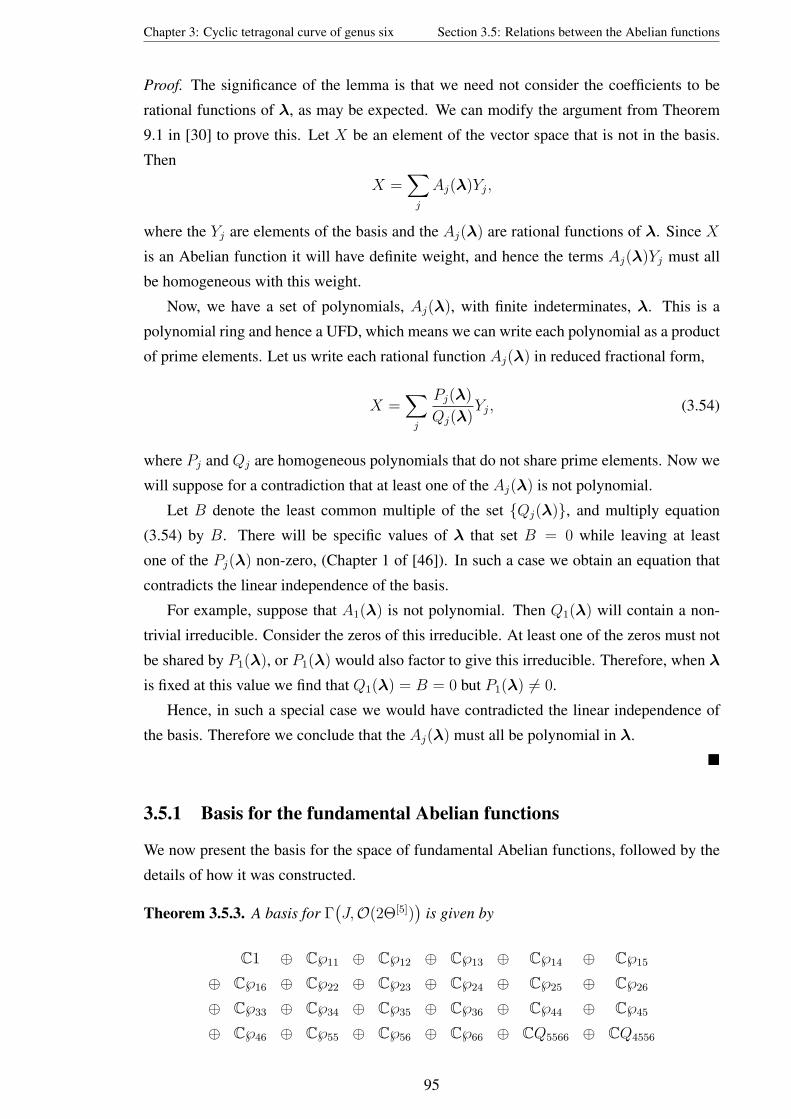
Chapter 3: Cyclic tetragonal curve of genus six Section 3.5: Relations between the Abelian functions
Proof. The significance of the lemma is that we need not consider the coefficients to be
rational functions of λ, as may be expected. We can modify the argument from Theorem
9.1 in [30] to prove this. Let X be an element of the vector space that is not in the basis.
Then
X =∑j
Aj(λ)Yj,
where the Yj are elements of the basis and the Aj(λ) are rational functions of λ. Since X
is an Abelian function it will have definite weight, and hence the terms Aj(λ)Yj must all
be homogeneous with this weight.
Now, we have a set of polynomials, Aj(λ), with finite indeterminates, λ. This is a
polynomial ring and hence a UFD, which means we can write each polynomial as a product
of prime elements. Let us write each rational function Aj(λ) in reduced fractional form,
X =∑j
Pj(λ)
Qj(λ)Yj, (3.54)
where Pj and Qj are homogeneous polynomials that do not share prime elements. Now we
will suppose for a contradiction that at least one of the Aj(λ) is not polynomial.
Let B denote the least common multiple of the set Qj(λ), and multiply equation
(3.54) by B. There will be specific values of λ that set B = 0 while leaving at least
one of the Pj(λ) non-zero, (Chapter 1 of [46]). In such a case we obtain an equation that
contradicts the linear independence of the basis.
For example, suppose that A1(λ) is not polynomial. Then Q1(λ) will contain a non-
trivial irreducible. Consider the zeros of this irreducible. At least one of the zeros must not
be shared by P1(λ), or P1(λ) would also factor to give this irreducible. Therefore, when λ
is fixed at this value we find that Q1(λ) = B = 0 but P1(λ) 6= 0.
Hence, in such a special case we would have contradicted the linear independence of
the basis. Therefore we conclude that the Aj(λ) must all be polynomial in λ.
3.5.1 Basis for the fundamental Abelian functions
We now present the basis for the space of fundamental Abelian functions, followed by the
details of how it was constructed.
Theorem 3.5.3. A basis for Γ(J,O(2Θ[5])
)is given by
C1 ⊕ C℘11 ⊕ C℘12 ⊕ C℘13 ⊕ C℘14 ⊕ C℘15
⊕ C℘16 ⊕ C℘22 ⊕ C℘23 ⊕ C℘24 ⊕ C℘25 ⊕ C℘26
⊕ C℘33 ⊕ C℘34 ⊕ C℘35 ⊕ C℘36 ⊕ C℘44 ⊕ C℘45
⊕ C℘46 ⊕ C℘55 ⊕ C℘56 ⊕ C℘66 ⊕ CQ5566 ⊕ CQ4556
95

Chapter 3: Cyclic tetragonal curve of genus six Section 3.5: Relations between the Abelian functions
⊕ CQ4555 ⊕ CQ4455 ⊕ CQ3566 ⊕ CQ3556 ⊕ CQ2566
⊕ CQ2556 ⊕ CQ3456 ⊕ CQ2456 ⊕ CQ3366 ⊕ CQ3445
⊕ CQ2366 ⊕ CQ2445 ⊕ CQ1466 ⊕ CQ1556 ⊕ CQ2266
⊕ CQ2356 ⊕ CQ2256 ⊕ CQ2346 ⊕ CQ1455 ⊕ CQ2345
⊕ CQ3344 ⊕ CQ2245 ⊕ CQ2344 ⊕ CQ1266 ⊕ CQ1356
⊕ CQ1444 ⊕ CQ1346 ⊕ CQ2236 ⊕ CQ2335 ⊕ CQ1246
⊕ CQ1255 ⊕ CQ1245 ⊕ CQ1166 ⊕ CQ1244 ⊕ CQ1156
⊕ CQ1146 ⊕ CQ1155 ⊕ CQ1145 ⊕ CQ1144 ⊕ CQ114466.
(3.55)
Proof. The dimension of the space is 2g = 26 = 64 by the Riemann-Roch theorem for
Abelian varieties. It was concluded above in equation (3.53) that all the selected elements
do in fact belong to the space. All that remains is to prove their linear independence, which
can be done explicitly using the σ-expansions in Maple.
The actual construction of the basis is as follows. We start by including all 21 of the
2-index ℘-functions in the basis, since they are all linearly independent. The next step is
to decide which 4-index Q-functions to include. We do this by systematically considering
weight levels, starting at −4 (the highest weight of any Q-function) and decreasing.
At each weight level we identify Qijkl to be added to the basis and derive equations for
the non-basis entries as a linear combinations of basis entries. This is achieved using the
following method, described for weight level −k, and implemented with Maple.
1. Start by forming a sum of existing basis entries, each multiplied by an undetermined
constant coefficient, ci. Note however that we need not include all the basis entries in
this sum, since the sum must be homogeneous of weight −k.
First include any basis entries at weight −k that have already been determined, (the
℘ij). Then include any elements with a higher weight, that may be multiplied by
an appropriate λ-monomial to balance the weight at −k overall. (Note that all the
possible elements of a higher weight have already been determined since we are
working systematically in decreasing weights.) Note also that from Lemma 3.5.2 we
need not consider basis entries multiplied by rational functions in the λ.
Note that we must account for the possibility of a constant term of weight −k. Such
a term must be a multiple of a λ-monomial at weight −k.
2. Add to this sum the Qijkl of weight−k, each multiplied by an undetermined constant
coefficient, qi.
3. Substitute the Abelian functions for their definitions as σ-derivatives. This will give
a sum of rational function which may be factored to leave σ(u)2 on the denominator.
(This is because the sum is a linear combination of functions with poles of order two
96

Chapter 3: Cyclic tetragonal curve of genus six Section 3.5: Relations between the Abelian functions
when σ(u) = 0.) Take the numerator, which should be a sum of products of pairs of
σ-derivatives.
4. Substitute σ(u) in this sum for the σ-expansion calculated in Section 3.4. Note that
the sum contains λ-monomials with weight no lower than −k. Hence we may trun-
cate the σ-expansion after the polynomial which contains λ-monomials of weight
−k. Evaluate the σ-derivatives as derivatives of this expansion.
5. Expand the pairs of products to obtain a polynomial. Note that this will create terms
with λ-monomials of a lower weight than −k. These terms must be discarded since
we would not have all such terms with this λ-monomial, (because we truncated the
expansion). Hence any information gained from them would be invalid.
6. Collect this polynomial into a sum of the various uλ-monomials with coefficients
in the unknown constants, ci, qi. Note that these coefficients will be linear in the
unknowns, (since the unknowns were from the original sum, not the expansions).
7. Consider these coefficients as a series of linear equations in the unknowns set to zero.
Since it is linear it is quite simple for a computer algebra package like Maple to solve.
• If there is a unique solution for the ci in terms of the qi then each of the Qijkl at
weight −k may be expressed as a linear combination of existing basis entries.
(To obtain the relations repeatedly set one of the qi to one and the others to zero
in the solution that was obtained.)
• However, it will more often be the case that this is not possible, and hence some
of the Qijkl must be selected as basis entries.
Suppose that there are x unknowns and (x − y) of the unknowns may be ex-
pressed using the other y. This means that specifying y of the qi determines
numerical values for all the ci and the other qi. Hence y of the Qijkl may be
expressed as a linear combination of basis entries and the other Qijkl. These
other Qijkl must be added to the basis.
There is usually several choices for which Qijkl to add to the basis, (since the
basis (3.55) is clearly not unique). However, we should check that the Qijkl
chosen are acceptable as in some special cases the Qijkl at a weight level may
be linear combinations of each other.
To obtain the relations for the non-basis Qijk repeatedly set one of the corre-
sponding qi to one and the others to zero in the solution that was obtained.
Hence we have identified the basis entries at weight −k and obtained relations for all
the non-basis entries as a linear combination of basis entries.
We give an example of this procedure for weight −8.
97

Chapter 3: Cyclic tetragonal curve of genus six Section 3.5: Relations between the Abelian functions
Example 3.5.4. Start by constructing the sum of existing basis entries. The entries at weight
−8 are ℘26 and ℘35. We additionally take the entries at weight −4 and combine them with
λ4. Finally we may have a constant at weight −8 so we need to include λ24 or λ3. We then
add to this sum the three Q-functions at weight 8 to end with the equation,
0 = c1℘26 + c2℘35 + c3℘46λ4 + c4℘55λ4 + c5λ24 + c6λ3
+ q1Q4466 + q2Q4556 + q3Q5555. (3.56)
We substitute the Abelian functions for σ-derivatives and take the numerator. We
then substitute in the σ-expansion truncated after C23, since this was the polynomial that
contained λ24 and λ3. Expanding the products of expansions will generate terms with
λ23, λ
24, λ3λ4, λ3λ
24 which must all be discarded. The polynomial that is left is collected
into uλ-monomials with coefficients in the unknowns. Setting these to zero and using the
Maple solve command we find a solution is given by
h1 = −72q3 + 6h4, h2 = −12q3 + h4, h3 = −64q3 + 4h4, h5 = 0,
h6 = −48q3 + 4h4, q1 = −16q3 + h4, q2 = −10q3 + h4,
for any values of h4 and q3. Therefore once two of the unknowns are determined the others
are established. This means that only two of the three Qijkl may be expressed as a linear
combination of the basis entries and the other Qijkl. We choose to add Q5566 to the basis.
To find the equations for the other two Qijkl first rearrange the equation for q1 above so that
it takes the role of h4.
h1 = 6q1 + 24q3, h2 = q1 + 4q3, h3 = 4q1, h4 = q1 + 16q3, h5 = 0,
h6 = 4q1 + 16q3, q2 = q1 + 6q3.
Then set q1 = 1, q3 = 0, substitute in (3.56) and rearrange to find
Q4466 = 6℘26 + ℘35 + 4λ4℘46 + λ4℘55 + 4λ3 −Q4556.
Similarly setting q1 = 0, q3 = 1 we find
Q5555 = 24℘26 + 4℘35 + 16λ4℘55 + 16λ3 − 6Q4556.
So we follow this procedure at successively lower weights, constructing the basis and
equations as we proceed. Note that after every four weight levels an additional Ck of the
σ-expansion is required. As discussed in Section 3.4 these relations were constructed in
tandem with the σ-expansion. Once a new Ck was found four more weight levels could be
98

Chapter 3: Cyclic tetragonal curve of genus six Section 3.5: Relations between the Abelian functions
examined. The relations obtained could then be used to construct the next Ck.
Note also that as the weight decreases, both the the possible number of terms in the
original sum and the size of the σ-expansion increase. Hence the computations take more
time and memory. The most computationally intensive part is Step 5 where the products of
expansions must be calculated and the terms with weight in λ lower than −k discarded.
• Since all the terms in the end polynomial contain an unknown, we should not use the
procedure described in the last section to perform this calculation, or we would lose
many constraints.
• However, we do find that the resulting system of linear equations for the unknowns
is very overdetermined. Hence we can simplify by setting some of the u to specific
values. We find that setting u = (u1, u2, 1, 1, 1, 1) achieves enough constraints to
specify the unknowns, while being computationally far simpler.
• To further save computation time and memory distributed computing may be em-
ployed to expand the pairs of products in parallel. This was implemented using the
Distributed Maple package, [72], discussed in Section 3.4.
Upon examining all the 4-index Q-functions, we find that 63 basis elements have been
identified. To find the final basis element we repeat the procedure using the 6-index Q-
functions. We find that all those of weight higher than −30 can be expressed as a linear
combination of existing basis entries. However, at weight−30 one of theQijklmn is required
in the basis to express the others. The Maple worksheets in which these calculations were
performed can be found in the extra Appendix of files.
3.5.2 Differential equations in the Abelian functions
We present a number of differential equations between the Abelian functions. The number
in brackets on the left indicates the weight of each equation.
Lemma 3.5.5. Those 4-index Q-functions not in the basis can be expressed as a linear
combination of the basis elements.
(−4) Q6666 = −3℘55 + 4℘46
(−5) Q5666 = −2℘45
(−6) Q4666 = 6λ4℘66 − 2℘44 − 32Q5566
(−7) Q4566 = 2λ4℘56 + 2℘36
(−7) Q5556 = 4λ4℘56 + 4℘36
(−8) Q4466 = 4λ4℘46 + λ4℘55 + ℘35 + 6℘26 −Q4556 + 4λ3
(−8) Q5555 = 16λ4℘55 + 4℘35 + 24℘26 − 6Q4556 + 16λ3
(−9) Q4456 = 83λ4℘45 + 2℘25 − 4
3℘34 − 1
6Q4555
99

Chapter 3: Cyclic tetragonal curve of genus six Section 3.5: Relations between the Abelian functions
(−9) Q3666 = 2λ4℘45 − 12Q4555
(−10) Q2666 = −12Q4455 − 1
2Q3566 − 1
2λ4Q5566 + 4℘66λ3
(−10) Q4446 = 6λ4℘44 − 2℘24 − 2λ24℘66 −Q4455 + 1
2λ4Q5566 − 5
2Q3566 + 4℘66λ3
(−11) Q3466 = 4℘36λ4 − 12Q3566
(−11) Q4445 = 6℘36λ4 − 2℘56λ24 + 8℘56λ3 − 3Q2566 − 3
2Q3556
(−12) Q2466 = 8℘16 − ℘33 + 2λ2 − 12Q2456 −Q3456 + 4λ4℘26 + 2λ4℘35
(−12) Q3555 = 24℘16 − 8℘33 + 16λ4℘35 − 6Q3456
(−12) Q4444 = −12℘16 + 9℘33 + 6λ2 + 12Q3456 + 12℘55λ3 + 4℘46λ24
− 16℘46λ3 − 3℘55λ24 + 12λ4℘26 − 18λ4℘35 − 6Q2556
...
The full list down to Q1111 can be found in the extra Appendix of files or online at [38].
There are similar equations for all the 6-index Q-functions, except Q114466 which is in
the basis. Explicit relations have been calculated down to weight −39. The first few are
given below while the full list can be found in the extra Appendix of files or online at [38].
(−6) Q666666 = 40℘44 + 15Q5566 − 24℘66λ4
(−7) Q566666 = 20℘36 − 4℘56λ4
(−8) Q556666 = 24℘26 − 12℘35 − 2Q4556
(−8) Q466666 = −20℘35 + 5Q4556 + 16℘46λ4 − 20℘55λ4 − 8λ3
(−9) Q456666 = −16℘25 + 83℘34 + 1
3Q4555 − 16
3℘45λ4
(−9) Q555666 = −16℘34 + 2Q4555 − 16℘45λ4
(−10) Q446666 = 8℘24 +Q4455 − 2Q3566 − 24℘44λ4 − 14Q5566λ4 + 40℘66λ24
(−10) Q455666 = −8℘24 − 4Q3566 + 2Q5566λ4 + 8℘66λ3
(−10) Q555566 = −16℘24 + 4Q4455 + 8Q3566 + 8Q5566λ4 − 16℘66λ3
(−11) Q366666 = −5Q3556 + 16℘36λ4
(−11) Q445666 = −6Q2566 + 3Q3556 + 12℘36λ4 + 4℘56λ24 + 8℘56λ3
(−11) Q455566 = −2Q3556 + 24℘36λ4 + 8℘56λ24
(−11) Q555556 = −20Q3556 + 112℘36λ4 + 16℘56λ24 + 32℘56λ3
...
Proof. By Theorem 3.5.3 and Lemma 3.5.2 it is clear such relations must exist. The explicit
differential equations were calculated in the construction of the basis, as discussed above.
100

Chapter 3: Cyclic tetragonal curve of genus six Section 3.5: Relations between the Abelian functions
Corollary 3.5.6. There are a set of differential equations that express 4-index ℘-functions
as a polynomial of Abelian functions of total degree at most two.
(−4) ℘6666 = 6℘266 − 3℘55 + 4℘46 (3.57)
(−5) ℘5666 = 6℘56℘66 − 2℘45 (3.58)
(−6) ℘4666 = 6℘46℘66 + 6λ4℘66 − 2℘44 − 32℘5566 + 3℘66℘55 + 6℘2
56
(−7) ℘4566 = 2℘45℘66 + 4℘46℘56 + 2λ4℘56 + 2℘36
(−7) ℘5556 = 6℘55℘56 + 4λ4℘56 + 4℘36
(−8) ℘4466 = 2℘44℘66 + 4℘246 + 4λ4℘46 + λ4℘55 + ℘35 + 6℘26
− ℘4556 + 4℘45℘56 + 2℘46℘55 + 4λ3
(−8) ℘5555 = 6℘255 + 16λ4℘55 + 4℘35 + 24℘26 − 6℘4556
+ 24℘45℘56 + 12℘46℘55 + 16λ3
(−9) ℘4456 = 2℘44℘56 + 4℘45℘46 + 83λ4℘45 + 2℘25 − 4
3℘34 − 1
6℘4555 + ℘45℘55
(−9) ℘3666 = 6℘36℘66 + 2λ4℘45 − 12℘4555 + 3℘45℘55
(−10) ℘2666 = −12℘4455 + ℘55℘44 + 2λ4℘
256 + ℘66λ4℘55 + ℘66℘35
+ 6℘26℘66 + 2℘245 + 2℘36℘56 − 1
2℘3566 − 1
2λ4℘5566 + 4℘66λ3
(−10) ℘4446 = 2℘55℘44 − 2℘24 − ℘4455 − 2λ24℘66 + 6λ4℘44 − 2λ4℘
256 − 5
2℘3566 + 4℘2
45
− ℘66λ4℘55 + 5℘66℘35 + 10℘36℘56 + 6℘46℘44 + 4℘66λ3 + 12λ4℘5566
...
Proof. Apply equation (3.32) to the first set of relations in Lemma 3.5.5 and rearrange.
The set of equations in Corollary 3.5.6 is of particular interest because it gives a general-
isation of Corollary 2.1.15 from the elliptic case. This was the elliptic differential equation
that allows higher order derivatives to be substituted out.
℘′′(u) = 6℘(u)2 − 12g2.
We discuss this generalisation more in Section 5.1 and present a full set of equations from
℘6666 to to ℘1111 in Appendix C.3. The other elliptic differential equation, which was de-
rived in Theorem 2.1.14, is
[℘′(u)]2 = 4℘(u)3 − g2℘(u)− g3.
A generalisation would be a set of equations that express the product of two 3-index ℘-
functions using a polynomial of fundamental Abelian functions with total degree at most
three. These are referred to as quadratic 3-index relations. For the cyclic-(4,5) curve these
101

Chapter 3: Cyclic tetragonal curve of genus six Section 3.5: Relations between the Abelian functions
relations have been derived for the first few weights and are presented below.
Note that the Q-functions present here were those included in the basis (3.55).
(−6) ℘2666 = 4℘3
66 + ℘256 + 4℘46℘66 − 4℘55℘66 − 4℘66λ4 + 4℘44 + 2Q5566
(−7) ℘566℘666 = 4℘266℘56 + 2℘46℘56 − ℘55℘56 − 2℘45℘66 + 2℘36
(−8) ℘2566 = 8℘26 + 4℘55λ4 + 4λ3 − 2Q4556 − 4℘45℘56 + 4℘2
56℘66 + ℘255
(−8) ℘556℘666 = 2℘256℘66 + 2℘46℘55 − 2℘2
55 − 4℘55λ4 + 2℘45℘56 + ℘66Q5566
+ 2℘55℘266 − 4℘26 − 2℘35 − 4λ3 + 2Q4556
(−8) ℘466℘666 = 4℘46℘266 + 4℘2
66λ4 + 2℘246 − 2℘46℘55 − 2℘55λ4 + ℘45℘56
− 2℘44℘66 − ℘66Q5566 − 2℘26 − 2℘35 − 2λ3 +Q4556
(−9) ℘556℘566 = ℘56Q5566 + 2℘66℘55℘56 + 2℘356 − 4
3℘45λ4 + 1
3Q4555 − 4
3℘34
(−9) ℘555℘666 = −2℘356 + 6℘66℘55℘56 + 4℘45℘46 + 8
3℘45λ4 − 4℘44℘56
− 3℘56Q5566 + 8℘36℘66 − 43℘34 − 2
3Q4555 − 4℘45℘55 + 8℘56℘66λ4
(−9) ℘466℘566 = 13Q4555 + ℘45℘55 − 2℘25 + 2
3℘34 + 4℘66℘46℘56 − ℘56Q5566
+ 4℘56℘66λ4 − 2℘44℘56 − 2℘45℘46 − 43℘45λ4
(−9) ℘456℘666 = 2℘66℘46℘56 + 2℘45℘266 + 2℘45℘46 + 4
3℘45λ4 + 2℘44℘56
+ 12℘56Q5566 + 2℘36℘66 − 2
3℘34 − 1
3Q4555 − 2℘45℘55 (3.59)
We do not give the details on the construction of these relations here, but instead refer the
reader to Chapter 5. This chapter deals with new results for the first trigonal cases including
a section on quadratic 3-index relations. The methods, problems and comments there are
also relevant for the (4,5)-case.
Proposition 3.5.7. There are a set of relations that are bi-linear in the 2-index and 3-index
℘-functions starting with the relations below.
(−6) 0 = −℘555 + 2℘456 + 2℘566℘66 − 2℘56℘666 (3.60)
(−7) 0 = −2℘446 + 2℘455 − 2℘466℘66 + 2℘666λ4 + 2℘46℘666
− 2℘556℘66 + ℘55℘666 + ℘566℘56
(−8) 0 = 2℘46℘566 − 2℘56℘466 + ℘555℘66 − 2℘55℘566 + ℘556℘56 − 2℘366
(−8) 0 = 2℘456℘66 − ℘445 + ℘56℘466 − ℘366 − ℘566λ4 − ℘45℘666 − 2℘46℘566
(−9) 0 = −2℘455℘66 + 4℘266 + 2℘45℘566 + 2℘466℘55 − 2℘46℘556
− ℘555℘56 + ℘556℘55 − 2℘356
(−10) 0 = 2℘256 − 4℘346 − 2℘446℘56 + 2℘44℘566 + 2℘45℘466 + ℘45℘556
− 2℘445℘66 − ℘455℘56
(−10) 0 = −2℘366℘66 + 2℘36℘666 + ℘45℘556 − 2℘346 + ℘355 − ℘455℘56
102

Chapter 3: Cyclic tetragonal curve of genus six Section 3.5: Relations between the Abelian functions
(−10) 0 = 6℘256 + ℘355 − 2℘456λ4 + ℘555λ4 + 2℘44℘566 + 4℘456℘46 − 2℘455℘56
+ 4℘45℘556 − 4℘456℘55 + 2℘46℘555 − 6℘346 − 2℘45℘466 − 4℘446℘56
(−11) 0 = ℘45℘555 − 4℘246 − 2℘445℘56 − 2℘446℘55 + 2℘46℘455 + 2℘255
− 2℘345 + 2℘44℘556 − ℘455℘55
(−11) 0 = 8℘666λ3 − 12℘266℘66 + 12℘26℘666 + 2℘35℘666 − 12℘246 + 6℘255
+ 2℘345 − 4℘445℘56 + 4℘45℘456 − 4λ4℘556℘66 + 2λ4℘55℘666
+ 2λ4℘566℘56 − 2℘46℘455 + 2℘44℘556 − 4℘356℘66 + 6℘36℘566
− ℘455℘55 + ℘45℘555 − 4℘56℘366,
(−12) 0 = −6℘344 − 10℘445λ4 + 4℘444℘56 − 8℘44℘456 − 4℘445℘46 + 8℘45℘446
+ 10℘356℘56 + 10℘46℘366 + 5℘55℘366 + 7λ4℘555℘66 − 14λ4℘55℘566
+ 7λ4℘556℘56 + 18℘245 − 10℘36℘466 − 2℘445℘55 + ℘45℘455
− 4℘366λ4 − 10℘566λ24 + 12℘566λ3 + 30℘26℘566 − 5℘35℘566
− 10℘36℘556 + ℘44℘555 − 30℘56℘266
(−13) 0 = 2℘34℘566 + 4℘36℘456 − ℘355℘56 + 2℘35℘556 − 2℘356℘55 + ℘36℘555
− 4℘336 − 2℘45℘366 − 4℘346℘56
Proof. The relations above can be calculated by cross differentiating suitable pairs of equa-
tions from Corollary 3.5.6. For example, equation (3.57) expresses ℘6666(u) while equation
(3.58) expresses ℘5666(u). If we substitute for these equations into
∂
∂u5
℘6666(u)− ∂
∂u6
℘5666(u) = 0,
then we find bilinear equation (3.60).
There is no analogue of Proposition 3.5.7 in the elliptic case, although similar relations
have been derived using the cross differentiation method in the hyperelliptic and trigonal
cases. Note that this method is much trickier in the (4,5)-case due to the large number
of Q-functions in the basis. This means that often more than two pairs of equations from
Corollary 3.5.6 need to be differentiated and examined. This gets increasing difficult at the
higher weights as there are more interrelated Q-functions.
In Chapter 5 we present a new method of deriving every bilinear relation associated
with a particular (n, s)-curve. This is used to complete the sets in the cyclic (3,4) and (3,5)-
cases. It was applied also to the cyclic (4,5)-case with all the bilinear relations that have
been derived available in the extra Appendix of files.
103

Chapter 3: Cyclic tetragonal curve of genus six Section 3.6: Addition formula
3.6 Addition formula
In this section we develop the two term addition formula for the σ-function. This gener-
alises Theorem 2.1.26 in the elliptic case which was first generalised by Baker in equation
(2.67) for a hyperelliptic function.
Theorem 3.6.1. The σ-function associated to the cyclic (4,5)-curve satisfies a two term
addition formula,
−σ(u+ v)σ(u− v)
σ(u)2σ(v)2= f(u,v)− f(v,u),
where f(u,v) is a finite polynomial of Abelian functions associated to C. It may be written
as
f(u,v) =[P30 + P26 + P22 + P18 + P14 + P10 + P6 + P2
](u,v),
where each Pk(u,v) is a sum of terms with weight −k in the Abelian functions and weight
k − 30 in λ-monomials.
Proof. We seek to express the following ratio of sigma functions, labeled LHS(u,v), using
a sum of Abelian functions.
LHS(u,v) = −σ(u+ v)σ(u− v)
σ(u)2σ(v)2. (3.61)
By Lemma 2.2.19 the σ-function has zeros of order one along Θ[5] and no zeros anywhere
else. This implies that LHS(u,v) has poles of order two along
(Θ[5] × J) ∪ (Θ[5] × J)
but nowhere else. Hence we can express LHS(u,v) as
LHS(u,v) =∑j
(c1jXj(u)Yj(v) + c2jXj(v)Yj(u)
), (3.62)
where theXj and Yj are functions chosen from the basis in Theorem 3.5.3 and the c1j, c2jare constant coefficients. A simple modification of Lemma 3.5.2 will show that these con-
stant coefficients must be polynomial functions of λ.
Recall Lemma 3.4.2 which stated that σ(u) is odd with respect to the change of vari-
ables u 7→ [−1]u. Now consider the effect of (u,v) 7→ (v,u) on LHS(u,v).
LHS(v,u) = −σ(u+ v)σ
([−1](u− v)
)σ(u)2σ(v)2
= −LHS(u,v).
So LHS(u,v) is antisymmetric, or odd with respect to the change (u,v) 7→ (v,u). Hence
we must have c2j = −c1j in equation (3.62) and equivalently LHS(u,v) can be written as
f(u,v)− f(v,u) for some function f .
104

Chapter 3: Cyclic tetragonal curve of genus six Section 3.6: Addition formula
Finally we use the fact that sigma has weight +15 to determine that the weight of
LHS(u,v) is −30. Hence we need only consider those from the basis (3.62) that may give
the correct overall weight. These will be the terms of weight−30 and the terms with higher
weight that be combined with an appropriate λ-monomial. This allows us to conclude that
the function f(u,v) may be split up as indicated in the theorem.
The formula is derived explicitly below. This is just the first of a family of similar
addition formula for the σ-function, related to the invariance expressed in equation (3.2).
Work has been conducted on the extra addition formula in the trigonal cases in [30]. In
[36] we see that this has inspired new results in the lower genus cases. Unfortunately such
addition formula cannot currently be derived for the (4,5)-case using this approach as it
requires the derivation of an additional basis and more polynomials in the σ-expansion,
which is not currently computationally feasible.
Constructing f(u, v)
We now describe how Maple was used to explicitly find f(u,v). (The corresponding Maple
worksheet is available in the extra Appendix of files.) First equation (3.62) is constructed
with the undetermined constants. This contains 1348 terms, but only 647 undetermined
coefficients due to the antisymmetry property. We may then determine the coefficients
using the σ-expansion, in a similar method to that described in the previous section.
We must substitute the Abelian functions for their definitions to give a sum of rational
function in σ-derivatives. We then take the numerator and substitute in the σ-expansion
truncated afterC43. (The addition formula may contain λ-monomials of weight−28, which
were contained in C43 of the σ-expansion.) We must then multiply out the products, discard
terms with weight in λ less than −28, collect the uvλ-monomials, set the coefficients to
zero and solve to find numerical values of the constants.
Note that the addition formula will have poles of order four and so we are required to
multiply the product of four large expansions. This can be difficult and there are a number
of techniques used for simplifying this problem.
• We design a procedure that is more efficient that the Maple expand command. We
cannot take the same approach of Section 3.4 and consider only the terms at a single
weight as there are unknowns at all weights. However, we can take a similar approach
and only multiply the terms that will not be discarded. To achieve this we categorise
the terms in the four expansions by their weights, and only consider the combinations
of four entries that result in an acceptable λ-weight.
• We may determine the conditions gradually by repeating the calculation, systemati-
cally adding Ck to the σ-expansion. For example, if we just use σ(u) = SW45 then
105

Chapter 3: Cyclic tetragonal curve of genus six Section 3.6: Addition formula
we identify the coefficients in P30. This causes much repetition of work, but can ease
the later calculations as many coefficients are found to be zero at each stage.
• The system of equations is again over-determined so it may be possible to use specific
values of u and v to ease computations.
• We again use distributed computing to expand the products in parallel. This was
implemented using Distributed Maple, [72].
We find that polynomials are given as below.
P2(u,v) = 73℘66(u)λ4λ3λ1 − 3
5℘66(u)λ2λ1 − 16
3℘66(u)λ3
4λ1 + 43℘66(u)λ2
4λ0
− 23℘66(u)λ3λ0
P6(u,v) = 163℘66(u)℘55(v)λ3λ1 + 7
12Q5566(v)λ4λ0 − 4℘46(u)℘66(v)λ2
4λ1
− 4℘46(v)℘66(u)λ3λ1 + 52℘55(u)℘66(v)λ4λ0 − 6℘55(v)℘66(u)λ2
4λ1 + 3℘44(u)λ3λ1
− 32Q5566(v)λ3λ1 + 4
3℘44(v)λ4λ0 − 16
3℘44(v)λ2
4λ1 − 2Q5566(v)λ24λ1
P10(u,v) =[5℘36(u)℘56(v)− 2℘24(v)− 5
3Q3566(v)− 5
2℘44(v)℘55(u)− 1
24Q4455(v)
− 52℘35(u)℘66(v) + 5
4Q5566(u)℘55(v)
]λ0 +
[4℘44(v)℘46(u) + 8
3℘24(v)
+ 185℘36(u)℘56(v) + 6℘26(v)℘66(u)− 11
2℘35(u)℘66(v) + 6℘44(v)℘55(u)
− 32Q5566(u)℘46(v) + 7
3Q5566(u)℘55(v)− 5
3Q3566(u)− 2
3Q4455(u)
]λ4λ1
P14(u,v) =[℘25(u)℘45(v) + 1
3Q3445(u) + 4
3℘14(v) + 5
12Q3366(v)− 11
20Q3556(u)℘56(v)
+ ℘22(u)− 6℘44(u)℘26(v) + 3Q5566(v)℘26(u) + 185℘16(u)℘66(v)− 7
3℘24(u)℘55(v)
+ 2312Q3566(v)℘55(u)− 1
24Q4555(u)℘45(v)− 27
10℘33(u)℘66(v)− 1
2Q4455(v)℘46(u)
− 35Q3456(u)℘66(v)− 2℘24(v)℘46(u) + 2
3Q4455(v)℘55(u)− 3℘35(u)Q5566(v)
− 23℘34(u)℘45(v)− 11
2℘35(u)℘44(v) + 3
10Q2556(u)℘66(v)− 3
2Q3566(v)℘46(u)
+ 110Q2566(v)℘56(u)
]λ1 +
[124Q3566(v)℘55(u) + 1
6℘25(u)℘45(v)− 1
10Q3556(u)℘56(v)
+ 16℘34(u)℘45(v)− 1
20Q2566(v)℘56(u)− 1
30Q3366(v)− 1
15Q3445(u) + 8
15℘14(v)
]λ4λ2
− 643℘16(v)℘66(u)λ4
4 + 683℘16(v)℘66(u)λ2
4λ3 − 323℘16(v)℘66(u)λ2
3
P18(u,v) =[
310Q2566(u)℘36(v)− ℘23(u)℘45(v)− 1
5Q2345(v) + 3
4℘56(u)Q2366(v)
+ 25℘12(u) + 1
24Q4555(u)℘25(v) + 4
3℘34(u)℘25(v)− 2℘45(u)℘15(v) + 1
3℘55(u)℘14(v)
− 124℘55(u)Q3445(v) + 1
6℘55(u)Q3366(v)− 1
24℘34(v)Q4555(u)− 3
5Q3556(u)℘36(v)
− 110Q3344(v)
]λ2 +
[720Q2566(u)℘36(v)− 3
5Q3556(u)℘36(v)− 1
4Q3566(u)℘35(v) + . . .
106

Chapter 3: Cyclic tetragonal curve of genus six Section 3.6: Addition formula
· · ·+ 13℘23(u)℘45(v)− 2
3℘16(v)Q5566(u)− 1
6℘45(u)℘15(v) + 2℘66(u)Q1556(v)
+ 2℘66(u)Q1466(v) + 43℘44(v)℘16(u)
]λ4λ3 +
[4℘66(u)Q1556(v)
+ 110Q2566(u)℘36(v) + 8℘16(v)Q5566(u) + 4℘66(u)Q1466(v)− 64
3℘44(v)℘16(u)
]λ3
4
P22(u,v) =[℘35(v)℘14(u) + 1
2℘15(v)℘25(u)− 58
15℘16(u)Q3566(v)− 1
2Q3366(v)℘35(u)
− 140Q2566(u)Q3556(v)− 1
5Q3456(u)Q3566(v)− 2Q1466(u)℘44(v)−Q1556(u)Q5566(v)
+ 2℘44(u)Q1556(v)−Q1466(v)Q5566(u)− 124℘23(u)Q4555(v) + 2
5℘33(u)Q3566(v)
+ 83Q1266(u)℘66(v) + 16
3Q1356(v)℘66(u)− 4
3℘23(v)℘34(u) + 1
10Q2556(u)Q3566(v)
+ 43Q1444(u)℘66(v) + 1
4Q3445(v)℘35(u)− 4
3℘16(u)Q4455(v)− 1
4Q2366(u)℘36(v)
− 4℘16(u)℘24(v)− 136℘15(u)℘34(v) + 1
24℘15(u)Q4555(v)− ℘23(v)℘25(u)
]λ3
+[3Q1266(u)℘66(v)− 6Q1356(v)℘66(u)− 1
15Q3456(u)Q3566(v)− 4℘44(u)Q1556(v)
− 32Q1466(v)Q5566(u)− 1
10Q2445(u)℘36(v) + 4Q1466(u)℘44(v) + 1
20Q2566(u)Q3556(v)
− 310℘33(u)Q3566(v) + 1
30Q2556(u)Q3566(v)− 4
3Q1444(u)℘66(v) + 3
2Q1556(u)Q5566(v)
+ 83℘16(u)Q4455(v) + 106
15℘16(u)Q3566(v) + 1
2Q2366(u)℘36(v) + 32
3℘16(u)℘24(v)
]λ2
4
P26(u,v) =[
124Q3566(u)Q2266(v)− 1
60Q2556(u)Q3366(v)− 1
2Q1556(u)Q4455(v)
−Q1146(u)− 76Q5566(v)Q1266(u) + 1
2Q1466(v)Q4455(u) + 1
30Q2556(u)Q3445(v)
− 115Q3445(v)Q3456(u)− 7
3Q5566(v)Q1356(u) + 7
6Q3566(u)Q1556(v)− ℘11(u)℘55(v)
− 12Q5566(u)Q1444(v) + 1
20Q3556(v)Q2445(u) + 1
6Q3566(u)Q2356(v) + 1
4Q1155(u)
− 130Q3456(v)Q3366(u) + 1
40Q2566(u)Q2445(v) + 7
6Q1466(v)Q3566(u)
+ 2Q1466(v)℘24(u)− 310Q3445(v)℘33(u) + 4
15Q2556(u)℘14(v)− 1
6℘45(u)Q1346(v)
− 12815℘16(v)℘14(u) + 2
5℘33(u)Q3366(v)− 8
15Q3366(v)℘16(u)− 1
24Q2335(u)℘45(v)
+ 2℘23(u)℘15(v) + 4℘16(v)℘22(u)− 125℘33(u)℘14(v)− 1
5℘36(u)Q2245(v)
+ 3℘44(u)Q1266(v) + 43℘44(v)Q1444(u) + 3
5℘36(v)Q2344(u)− 2℘25(u)℘13(v)
− 2℘35(u)℘12(v) + 124℘45(u)Q2236(v)− 8
15Q3456(u)℘14(v)− ℘66(v)Q1244(u)
+ 1415℘16(v)Q3445(u) + 6℘44(u)Q1356(v)− 2Q1556(u)℘24(v)
]λ4
P30(u,v) = 14Q114466(u) + 5
3Q3566(v)Q1356(u)− 1
3℘14(v)Q2356(u) + 1
3Q1556(v)℘14(u)
+ 110Q3344(v)Q3456(u)− 1
2℘25(v)Q1346(u) + 1
2Q4556(v)℘11(u)− 1
4Q2236(u)℘25(v)
+ 35Q3344(u)℘16(v) + 1
24Q1346(v)Q4555(u) + 1
2Q1145(v)℘56(u)− 2
5Q2345(u)℘33(v)
− 12Q1556(v)℘22(u) + 1
2Q1155(u)℘46(v) + 5
6Q3566(v)Q1266(u) + 1
12Q2236(v)℘34(u)
+ 75℘12(v)Q3456(u)− 2
3Q1356(v)Q4455(u)− 1
20Q2245(v)Q2566(u) + . . .
107

Chapter 3: Cyclic tetragonal curve of genus six Section 3.6: Addition formula
· · ·+ 13Q1466(u)Q3445(v)− 4
3Q1466(u)℘14(v)− ℘26(v)℘11(u) + ℘36(v)Q1245(u)
+ 110Q2345(u)Q2556(v) + ℘26(v)Q1246(u) +Q2346(v)℘15(u) + 1
2Q1444(v)Q3566(u)
+ 15℘16(v)Q2345(u)− 1
12Q3445(v)Q2266(u) + 1
2Q5566(v)Q1244(u)− 1
5℘33(v)Q3344(u)
+ 16Q1466(v)Q3366(u) + 1
48Q4555(v)Q2335(u) + 1
3Q4455(v)Q1266(u) +Q1246(v)℘35(u)
− 16Q4455(v)Q1444(u) + 1
5Q2345(v)Q3456(u) + 1
2Q1156(v)℘45(u)− ℘46(v)Q1146(u)
+Q2256(v)℘15(u)− 325℘12(v)℘16(u)− 7
3Q1356(v)℘24(u)− 1
2℘33(v)Q1455(u)
− 148Q2236(v)Q4555(u)− 1
20Q3344(v)Q2556(u)− 1
10Q2566(v)Q2344(u)
− 110Q3556(v)Q2245(u)− 1
20Q3556(v)Q2344(u) + 1
8Q2445(v)Q2366(u)
+ 16Q1556(v)Q3366(u)− 1
2Q1255(u)℘26(v)− 1
2Q1144(v)℘66(u) + 1
2℘44(v)Q1166(u)
− 512Q2335(v)℘34(u) + 1
6Q3366(v)Q2266(u) + 2
3℘24(v)Q1266(u)−Q1455(v)℘16(u)
− 12Q2256(v)℘23(u)− ℘22(u)Q1466(v) + 1
2℘55(v)Q1146(u)−Q2346(v)℘23(u)
+ 16Q1346(u)℘34(v)− 1
3℘14(u)Q2266(v) + ℘13(v)Q2456(u) + 14
5℘33(u)℘12(v)
− 15℘12(v)Q2556(u)− 2
3℘24(v)Q1444(u) + 1
4Q2335(v)℘25(u) + ℘44(v)Q1244(u)
− 13Q2356(v)Q3366(u) + 1
3Q3445(v)Q1556(u)− 1
6Q3445(v)Q2356(u)− ℘35(v)℘11(u).
Note that the 6-index Q-function in basis (3.55) is present in P30 and was essential for the
construction of the addition formula.
The two term addition formulae are the only results in this document that will change
with a different choice of c in the definition of the σ-function, (see Remark 2.2.23). Using
an alternative constant will change the polynomial f(u,v) by a multiplicative constant
factor, (see Appendix B).
108

Chapter 3: Cyclic tetragonal curve of genus six Section 3.7: Applications in the KP hierarchy
3.7 Applications in the KP hierarchy
The Weierstrass ℘-function had applications in many areas of mathematics, (see for exam-
ple [3]). It may be used to construct solutions for problems such as the pendulum equation,
and in particular the function,
W (x, t) = A℘(x− ct) +B,
gives a traveling wave solution to the KdV equation,
Wt + 12WWx +Wxxx = 0.
A similar application may be derived from Baker’s results on the Kleinian ℘-functions
associated to a (2,5)-curve. In [10] (page 47 of the reprinted edition) Baker derived the
following equation between the hyperelliptic ℘-functions.
℘2222 − 6℘222 =
1
2λ3 + λ4℘22 + 4℘12.
We make the change of variables u1 = T, u2 = x to get
℘xxxx − 6℘2xx =
1
2λ3 + λ4℘xx + 4℘Tx.
We then differentiate with respect to x.
℘xxxxx − 12℘xx℘xxx = λ4℘xxx + 4℘Txx.
Now set λ4 = 0, t = −4T and define W (x, t) = −℘xx(x, t). Then W (x, t) is a solution of
0 = Wt + 12WWx +Wxxx.
So Baker had constructed a 2-soliton solution to the periodic KdV equation.
More recently, in [21] and [35], the cyclic trigonal curves have been linked to the
Boussinesq equation. In [11] the ℘-functions associated to the cyclic (3,5)-curve are shown
to satisfy
℘4444 = 6℘244 − 3℘33.
Differentiate twice with respect to u4 to give the Boussinesq equation for ℘44, with u4
playing the role of the space variable and u3 the time variable.
Given these results it is not surprising to see a similar result occurring in the cyclic
(4,5)-case. This time a solution to the KP-equation can be constructed.
109

Chapter 3: Cyclic tetragonal curve of genus six Section 3.7: Applications in the KP hierarchy
Recall equation (3.57) derived in Corollary 3.5.6.
℘6666 = 6℘266 − 3℘55 + 4℘46.
Differentiate twice with respect to u6 to obtain
℘666666 = 12∂
∂u6
(℘66℘666
)− 3℘5566 + 4℘4666. (3.63)
This time we use the substitutions u6 = x, u5 = y, u4 = t and define the function
W (x, y, t) = ℘xx(u1, u2, u3, t, y, x).
Substituting into equation (3.63) and rearranging will show that W (x, y, t) is a solution of
to the following form of the KP-equation.
[Wxxx − 12WWx − 4Wt
]x
+ 3Wyy = 0.
In fact this is just a special case of the following general result for Abelian functions asso-
ciated with algebraic curves.
Theorem 3.7.1. Let C be an (n, s)-curve with genus g as defined by equation (2.34). De-
fine the σ-function and Abelian functions associated with C as normal. Finally define the
function W (u) = ℘gg(u), which we may denote W (x, y, t) after applying the substitutions
ug = x, ug−1 = y, ug−2 = t.
Then, if n ≥ 4, the functionW (x, y, t) will satisfy the following version of the KP-equation.
(Wxxx − 12WWx − bWt
)x− aWyy = 0, (3.64)
for some constants a, b.
Proof. Recall Definition 3.3.2 and Theorem 3.3.4 which gave the Sato weights for C. The
weights of the variables u were the entries in the Weierstrass gap sequence generated by
(n, s). These are the natural numbers not representable in the form αn+βswhere α, β ∈ N.
Since s > n > 4 we know that 1, 2, 3 cannot be represented in this form. Therefore
we have
weight(ug) = +1, weight(ug−1) = +2, weight(ug−2) = +3.
By Lemma 3.3.10 this implies the 2-index ℘-functions will have weights
wt(℘g,g) = −2, wt(℘g,g−1) = −3, wt(℘g−1,g−1) = −4, wt(℘g−2,g) = −4,
110

Chapter 3: Cyclic tetragonal curve of genus six Section 3.7: Applications in the KP hierarchy
with all the other 2-index ℘-functions having a lower weight.
Next consider Qgggg, which by Lemma 3.3.14 is the highest weight Q-function with
weight−4. We noted in Section 3.5 that theQ-functions all belong to Γ(J,O(2Θ[g−1])
), the
space of Abelian functions associated to C with poles of at most order 2 when u ∈ Θ[g−1].
By Lemma 3.5.2 we can express Qgggg as
Qg,g,g,g = a℘g−1,g−1 + b℘g−2,g + c, (a, b, c constants),
since these are the only Abelian functions of weight −4, and there is no function of lower
weight that could be combined with a λ-monomial to give the correct weight. We use
Definition 3.1.2 to substitute Qgggg for its expression in ℘-functions.
℘g,g,g,g − 6℘2g,g = a℘g−1,g−1 + b℘g−2,g + c.
Then differentiate twice with respect to ug to give
℘g,g,g,g,g,g = 12 ∂∂ug
(℘g,g℘g,g,g
)+ a℘g−1,g−1,g,g + b℘g−2,g,g,g.
Then make the substitutions suggested in the theorem to obtain equation (3.64).
Hence the Abelian functions associated to the cyclic (n, s)-curve with n > 4 may all
be used to construct solutions to the same KP-equation as those functions associated to the
cyclic tetragonal curve of genus six.
111

Chapter 4
Higher genus trigonal curves
The results of Chapter 3 required the development of new techniques, methods and the
corresponding Maple programs. In this Chapter we have applied these to generate results
for the higher genus trigonal curves. In most cases the same methods and programs could
be used with only slight modifications and hence we do not repeat the discussion of these.
We start in Section 4.1 by investigating the Abelian functions associated to the cyclic
(3,7)-curve. This curve has genus g = 6, the same as the cyclic (4,5)-curve investigated in
Chapter 3. It will be interesting to see whether the theory is more closely related to that of
the lower genus trigonal curves studied in [30] and [11] or to that of the (4,5)-curve with
which there is a shared genus.
Next, in Section 4.2 we repeat the process for the cyclic (3,8)-curve which has genus
g = 7 and is the highest genus curve to have been considered. The Maple worksheets that
were used to derive results can be found in the extra Appendix of files.
The main motivation for the investigation of these two higher genus curves is to facili-
tate with the future construction of a general theory for the trigonal curve. However, they
also have potential applications in both integrable systems and the theory of Weierstrass
semigroups.
112

Chapter 4: Higher genus trigonal curves Section 4.1: The cyclic trigonal curve of genus six
4.1 The cyclic trigonal curve of genus six
In this section we present results for the Abelian functions associated with the cyclic (3,7)-
curve. This is the curve C given by
y3 = x7 + λ6x6 + λ5x
5λ4x4 + λ3x
3 + λ2x2 + λ1x+ λ0. (4.1)
Using equation (2.33) we find this curve has genus g = 6. (Note this curve has the same
genus as the cyclic (4,5)-curve investigated in Chapter 3.)
4.1.1 Differentials and functions
We need to start by investigating the differentials on C. Recalling Definition 2.2.3 we
construct the Weierstrass gap sequence generated by (n, s) = (3, 7).
W3,7 = 1, 2, 4, 5, 8, 11, W 3,7 = 3, 6, 7, 9, 10, 12, 13, . . . . (4.2)
We follow Proposition 2.2.4 to construct the basis of holomorphic differentials upon C.
du = (du1, . . . , du6), where dui(x, y) =gi(x, y)
3y2dx,
withg1(x, y) = 1, g2(x, y) = x, g3(x, y) = x2,
g4(x, y) = y, g5(x, y) = x3, g6(x, y) = xy.(4.3)
Any point u ∈ C6 can be expressed as
u = (u1, u2, u3, u4, u5, u6) =6∑i=1
∫ Pi
∞du, (4.4)
where the Pi are six variable points upon C.
Next we must construct the fundamental differential of the second kind, (Definition
2.2.6). We follow Klein’s explicit realisation set out in Proposition 2.2.8 and find that the
fundamental differential may be expressed as
Ω((x, y), (z, w)
)=F((x, y), (z, w)
)dxdz
9(x− z)2y2w2, (4.5)
where F is the following symmetric polynomial.
F((x, y), (z, w)
)= 2λ1yz + λ2x
2w + 2λ1wx+ 3wλ0 + 3xλ3yz2 − yz4λ4
+ 2x2yz3λ5 + 4xyz3λ4 + yz4xλ5 + λ2yz2 + 3yz4x2λ6 + 3x4wλ6z
2 + yz4x3
+ 2x3wλ5z2 + 2x5wz2 + 2x2yz5 + x4wz3 + 3y2w2 + λ1yx+ λ1wz + 3yλ0
+ λ5x4wz − λ4x
4w + 2λ2xwz + 2λ2xyz + 3λ3x2wz + 4λ4x
3wz. (4.6)
113

Chapter 4: Higher genus trigonal curves Section 4.1: The cyclic trigonal curve of genus six
(See Section 3.1.1 for a detailed example of such a construction.)
In obtaining the realisation, an explicit basis for the differentials of the second kind
associated with the cyclic (3,7)-curve was derived.
dr = (dr1, . . . , dr6), where drj(x, y) =hj(x, y)
3y2dx, (4.7)
with
h1(x, y) = y(9x4λ6 + 5x2λ4 + 11x5 + λ2 + 3xλ3 + 7x3λ5
),
h2(x, y) = xy(4xλ5 + 6x2λ6 + 8x3 + 2λ4
),
h3(x, y) = y(5x3 − λ4 + xλ5 + 3x2λ6
),
h4(x, y) = x3(3xλ6 + 4x2 + 2λ5
),
h5(x, y) = 2x2y,
h6(x, y) = x4.
We can now proceed to define Abelian functions as in the general case. Start by choos-
ing an appropriate basis of cycles upon the surface defined by C. (Ensure condition (2.45)
on the intersection numbers is satisfied.) Then define the period matrices as in equations
(2.46) and (2.52) by integrating the differentials (4.3) and (4.7) around these cycles.
Let Λ denote the lattice generated by the first pair of period matrices, (Definition 2.2.10),
and define an Abelian function associated withC as a meromorphic function that is periodic
over this lattice, (Definition 2.2.11). Define the Jacobian as the complex space modulo this
lattice, (Definition 2.2.12) and recall Definition 2.2.13 for the Abel map.
A : Symk(C)→ J
(P1, . . . , Pk) 7→(∫ P1
∞du+ · · ·+
∫ Pk
∞du
)(mod Λ), (4.8)
where the Pi are points upon C. Finally by Definition 2.2.14 the strata of the Jacobian are
the images of the Abel map.
When k = 1 the Abel map gives an embedding of the curve C upon which we define ξ
as the local parameter at the origin, A1(∞).
ξ = x−13 . (4.9)
We can derive series near the origin in ξ for the key variables.
x =1
ξ3,
dx
dξ= − 3
ξ4,
y =1
ξ7+
(λ6
3
)1
ξ4+
(λ5
3− λ2
6
9
)1
ξ+
(λ4
3− 2λ6λ5
9+
5λ36
81
)ξ2 +O
(ξ5).
114

Chapter 4: Higher genus trigonal curves Section 4.1: The cyclic trigonal curve of genus six
du1 = [−ξ10 +O(ξ13)]dξ, du4 = [−ξ3 +O(ξ6)]dξ,
du2 = [−ξ7 +O(ξ10)]dξ, du5 = [−ξ1 +O(ξ4)]dξ,
du3 = [−ξ4 +O(ξ7)]dξ, du6 = [−1 +O(ξ3)]dξ.
u1 = − 111ξ11 +O(ξ14), u3 = −1
5ξ5 +O(ξ8), u5 = −1
2ξ2 +O(ξ5),
u2 = −18ξ8 +O(ξ11), u4 = −1
4ξ4 +O(ξ7), u6 = −ξ +O(ξ4).
(4.10)
We will work with the Abelian functions derived from the Kleinian σ-function associ-
ated with the (3, 7)-curve. This is defined as in Definition 2.2.15 and is here a function of
g = 6 variables.
σ = σ(u) = σ(u1, u2, u3, u4, u5, u6).
The Schur-Weierstrass polynomial can be constructed as in Example A.5.21.
SW3,7 = 122528000
u166 + u2
2 + 180u4u
66u
35 + 1
3200u4u
106 u5 + 1
8u2
6u55u4 − 1
2u3u
36u
24
+ 12u2
6u5u34 − 1
16u2
4u46u
25 + u6u
25u1 − 1
2u2u
26u
35 − u2u
25u4 + 1
40u2u
66u5 − 1
20u5
6u1
− 180u7
6u25u3 + 1
2u2
3u26u
25 + 1
8u3u
36u
45 + 2u5u4u
23 + 3
8u4
5u24 − 1
640u2
4u86 + 1
4u4u
46u2
− u3u6u35u4 − 1
64u8
5 − 120u4u
56u3u5 + 1
2560u8
6u45 − 1
4u4
4 − u3u1 − 2u2u3u6u5
− 135200
u3u116 + u6u
33 − 3
281600u12
6 u25 − 1
64u6
5u46 + 1
40u2
3u66 (4.11)
Recall that this polynomial is the canonical limit of the σ-function.
Define the n-index ℘-functions associated with the (3, 7)-curve as in Definition 2.2.27.
Since the genus is six there will be the same number of ℘-functions as in the (4,5)-case. We
will also need to use the n-index Q-functions as defined in Section 3.1.3.
In Section 3.3 we proved that all the objects in the theory associated with any (n, s)-
curve may be given a weight so that all equations are homogeneous. In the case of the
cyclic (3,7)-curve these weights are as follows.
+x +y +λ6 +λ5 +λ4 +λ3 +λ2 +λ1 +λ0
Weight −3 −7 −3 −6 −9 −12 −15 −18 −21space
u1 u2 u3 u4 u5 u6 σ(u)
Weight +11 +8 +5 +4 +2 +1 +16
Note that as always the local parameter ξ has weight one, while the weights of the ℘-
functions andQ-functions may be derived from their indices as described in Lemmas 3.3.12
and 3.3.14.
115

Chapter 4: Higher genus trigonal curves Section 4.1: The cyclic trigonal curve of genus six
Note that while we have the same ℘-functions as in the (4,5)-case, their weights are
different.
weight[℘11] = −22 weight[℘23] = −13 weight[℘36] = −6
weight[℘12] = −19 weight[℘24] = −12 weight[℘44] = −8
weight[℘13] = −16 weight[℘25] = −10 weight[℘45] = −6
weight[℘14] = −15 weight[℘26] = −9 weight[℘46] = −5
weight[℘15] = −13 weight[℘33] = −10 weight[℘55] = −4
weight[℘16] = −12 weight[℘34] = −9 weight[℘56] = −3
weight[℘22] = −16 weight[℘35] = −7 weight[℘66] = −2
(Compare with Example 3.3.11 for the (4,5)-case).
4.1.2 Expanding the Kleinian formula
We need to derive relations between the ℘-functions from the Kleinian formula, (Theorem
3.2.1). We discussed the procedure to do this in detail in Section 3.2. As before, we use the
expansions of the variables in ξ to expand equation (3.33) as a series in ξ. The coefficients
are polynomials in the variables (z, w) and the ℘-functions, starting with the five below.
0 = ρ1 = −z4 + ℘56z3 + ℘36z
2 +(℘66w + ℘26
)z + ℘46w + ℘16 (4.12)
0 = ρ2 =(℘55 − ℘566
)z3 +
(℘35 − 2w − ℘366
)z2 +
(℘25 − ℘266 + ℘56w
− ℘666w)z + ℘15 − ℘466w − ℘166 + ℘45w (4.13)
0 = ρ3 =(
12℘5666 − 3
2℘556
)z3 +
(12℘3666 − 3
2℘356
)z2 +
(12℘2666 − 3
2℘256
+ (12℘6666 − 3
2℘566)w
)z − 3
2℘156 − 3w2 + 1
2℘1666 +
(− 3
2℘456 + 1
2℘4666
)w
0 = ρ4 = −2z5 −(2℘56 + 10
3λ6
)z4 +
(13℘56λ6 + ℘5566 − 1
6℘56666 − 1
2℘555 − 2℘36
− 2λ5 + ℘45
)z3 +
(℘3566 − 2℘26 − 2℘66w − 1
2℘355 + ℘34 + 1
3℘36λ6 − 1
6℘36666
)z2
+(℘2566 − 1
6℘26666 − 2℘16 + 1
3℘26λ6 − 1
2℘255 +
(13℘66λ6 − ℘46 − 1
6℘66666
− 12℘556 + ℘5666
)w + ℘24
)z +
(℘4566 − 1
6℘46666 + ℘44 + 1
3℘46λ6 − 1
2℘455
)w
+ 13℘16λ6 + ℘14 − 1
2℘155 + ℘1566 − 1
6℘16666
0 = ρ5 =(2℘566 − 2℘55
)z4 +
(58℘5556 − 5
12℘55666 + 2℘366 − ℘35 − 5
4℘456 − w
+ 124℘566666 − 1
4℘566λ6
)z3 +
((2℘666 − 3λ6 − 2℘56
)w − 5
12℘35666 + 2℘266
+ 124℘366666 + ℘33 + 5
8℘3556 − 1
4℘366λ6 − 2℘25 − 5
4℘346
)z2 +
(2℘166 − 5
4℘246
− 14℘266λ6 + ℘23 − 5
12℘25666 − 2℘15 + 5
8℘2556 +
(℘36 − 2℘45 + 5
8℘5566 − 5
12℘56666
+ 34℘466 − λ5 + 1
24℘666666 − 1
4℘666λ6)w + 1
24℘266666
)z +
(− 1
4℘466λ6 + 5
8℘4556
− 512℘45666 − 5
4℘446 + 1
24℘466666 + λ4 + ℘34
)w − 5
12℘15666 + 5
8℘1556 − 1
4℘166λ6
+ ℘13 + 124℘166666 − 5
4℘146
116

Chapter 4: Higher genus trigonal curves Section 4.1: The cyclic trigonal curve of genus six
They are valid for any u ∈ C6, with (z, w) one of the point on C that are used in equation
(4.4) to represent u. They are presented in ascending order (as the coefficients of ξ) and
have been calculated explicitly, (using Maple), up to ρ10. They get increasingly larger in
size and can be found in the extra Appendix of files.
As described in Section 3.2 we next take resultants of pairs of equations, eliminating
the variable w by choice. (See Appendix A.6 for an introduction to resultants.) We denote
the resultant of ρi and ρj by ρi,j . These equations are quite large and not presented here.
Instead we present Table 4.1 detailing the number of terms they contain once expanded and
their degree in z.
Table 4.1: The polynomials ρi,j
Res # terms degree Res # terms degreeρ1,2 40 6 ρ3,4 2025 10ρ1,3 79 8 ρ3,5 4188 9ρ1,4 77 6 ρ3,6 4333 8ρ1,5 154 7 ρ3,7 19043 10ρ1,6 344 8 ρ3,8 28422 10ρ1,7 290 7 ρ3,9 44409 10ρ1,8 412 7 ρ4,5 793 8ρ1,9 1055 8 ρ4,6 8315 10ρ2,3 307 7 ρ4,7 1183 8ρ2,4 219 7 ρ4,8 2112 8ρ2,5 226 6 ρ4,9 24569 10ρ2,6 1468 8 ρ5,6 18356 10ρ2,7 712 7 ρ5,7 2535 8ρ2,8 737 7 ρ5,8 2316 8ρ2,9 4536 9 ρ5,9 54384 11
In general, the higher the ρi involved in the resultant, the more terms the resultant would
have. There were only two polynomials found with degree six in z, ρ12 and ρ14, with all the
others having higher degree. Recall that in the (4,5)-case the corresponding polynomials
had much more terms and all had degree in z of at least seven.
With regards to the expansion of the Kleinian formula, the (3,7)-case has far more in
common with the lower genus trigonal curves that the other higher genus curves that share
the genus. This was partly predicted by the results of [21].
Next recall the result of Theorem 3.2.2 on equations between the ℘-functions and a
point z on the curve from which they are defined. It stated that such an equation with degree
g − 1 = 5 in z must be identically zero. We hence aim to manipulate these polynomials to
achieve this.
117

Chapter 4: Higher genus trigonal curves Section 4.1: The cyclic trigonal curve of genus six
We select ρ1,2 as it is the smallest polynomial of degree six, and rearrange it to give an
equation for z6.
z6 = −12z5℘666 − 1
2℘2
56z4 − 1
2℘16℘45 + 1
2℘16℘466 + ℘16z
2 − 12℘166℘46 − 1
2℘166z℘66
− 12z2℘26℘56 + 1
2℘15℘46 + 3
2z5℘56 + 1
2z2℘26℘666 − 1
2z4℘466 + 1
2z℘16℘666 + z3℘26
+ 12z2℘25℘66 + 1
2z3℘35℘66 − 1
2z4℘566℘66 − 1
2z℘266℘46 + 1
2z4℘55℘66 − 1
2z3℘566℘46
+ 12℘36z
2℘466 + 12z℘26℘466 − 1
2z℘26℘45 + ℘36z
4 − 12℘16z℘56 + 1
2z4℘45 + 1
2z℘25℘46
− 12℘36z
3℘56 + 12℘36z
3℘666 + 12℘56z
4℘666 + 12℘56z
3℘466 − 12℘56z
3℘45 − 12℘36z
2℘45
− 12z2℘266℘66 + 1
2z3℘55℘46 + 1
2z2℘35℘46 + 1
2℘15z℘66 − 1
2z2℘366℘46 − 1
2z3℘366℘66.
We may now take any of the other ρi,j and repeatedly substitute for z6 until we have a
polynomial of degree five in z. By Theorem 3.2.2 the coefficients, with respect to z, of
such an equation must be zero. Further, since they are zero we can take the numerator of
the coefficients leaving us with six polynomial equations between the ℘-functions. Finally,
recalling Lemma 2.2.32 which stated that all the ℘-functions have definite parity, we can
separate each of these six relations into their odd and even parts. We denote the polyno-
mial equations between ℘-functions that we generate using this method by K(ρi,j, n,±) as
defined in Definition 3.2.3.
In the (4,5)-case every polynomial needed at least two rounds of substitution, and the
equations for z6 and z7 were far more complicated. In this case we need only substitute
once into ρ14 and so the polynomials achieved here are far simpler.
K(ρ14, 5,+) =(2℘666 − 3λ6 − 6℘56
)℘66 + ℘5666 − 3℘46
K(ρ14, 5,−) = −12℘556 − 1
6℘66666
K(ρ14, 4,+) =(2℘566 − 2℘55
)℘2
66 +(℘5566 − ℘45 − 2λ5 − 4℘36 + 2℘466
− 2℘56℘666 + 2℘256
)℘66 + ℘44 + ℘4566 − ℘56℘5666 − ℘56℘46 − 3℘46λ6
K(ρ14, 4,−) = −(
16℘56666 + 1
2℘555
)℘66 − 1
6℘46666 + 1
2℘56℘556
+ 16℘56℘66666 − 1
2℘455
...
However, the other relations all involve two rounds of substitution for z6 and get increas-
ingly long and complex, involving higher index ℘-functions.
Although the relations we achieve are far simpler than those in the (4,5)-case, there
do not seem to be enough simple relations to manipulate to find the desired differential
equations between the ℘-functions. Hence we proceed to use the tools developed for the
(4,5)-curve to find these relations.
However, as predicted by [21], we may still use the relations from the Kleinian formula
to find the solution of the Jacobi Inversion Problem.
118

Chapter 4: Higher genus trigonal curves Section 4.1: The cyclic trigonal curve of genus six
Recall that the Jacobi Inversion Problem is, given a point u ∈ J , to find the preimage
of this point under the Abel map (4.8).
Theorem 4.1.1. Suppose we are given u1, . . . , u6 = u ∈ J . Then we could solve the
Jacobi Inversion Problem explicitly using the equations derived from the Kleinian formula.
Proof. Consider the polynomial ρ12 which had degree six in z. Denote by (z1, . . . , z6)
the six zeros of the polynomial, which will be expressions in ℘-functions. Next consider
equation (4.12) which is degree one in w. Substitute each zi into equation (4.12) in turn
and solve to find the corresponding wi.
Therefore the set of points (z1, w1), . . . , (z6, w6) on the curve C which are the Abel
preimage of u have been identified.
4.1.3 The σ-function expansion
We construct a σ-function expansion for the cyclic (3,7)-curve using the methods and tech-
niques discussed in detail in Section 3.4. We start with a statement on the structure of the
expansion.
Theorem 4.1.2. The function σ(u) associated with the cyclic (3,7)-curve may be expanded
about the origin as
σ(u) = σ(u1, u2, u3, u4, u5, u6) = SW3,7(u) + C19(u) + C22 + · · ·+ C16+3n(u) + · · ·
where each Ck is a finite, even polynomial composed of products of monomials in
u = (u1, u2, . . . , u6) of weight +k multiplied by monomials in λ = (λ6, λ5, . . . , λ0) of
weight 16− k.
Proof. This is very similar to the proof of Theorem 3.4.3. First we note that the σ-function
associated with the (3,7)-curve is even by Lemma 2.2.20. Then by Theorem 3(i) in [60] we
know the expansion will be a sum of monomials in u and λ with rational coefficients.
We split the expansion into terms with common weight ratios. By Lemma 3.3.7 we
know that σ(u) has weight +16 and by Theorem 2.2.21 we know that the part of the ex-
pansion without λ will be SW3,7. We then have a sum of other polynomials with increasing
weight in u. The subscripts increase by three since the possible weights of λ-monomials
decrease by three.
We presented SW3,7 earlier in equation (4.11). We construct the other Ck successively
following the steps set out in Section 3.4. The same Maple procedures could be easily
adapted to perform the calculations.
119

Chapter 4: Higher genus trigonal curves Section 4.1: The cyclic trigonal curve of genus six
Note that those polynomials up to and including C39 required the use of method (III)
— ensuring polynomials derived from the expansions of the Kleinian formula in the last
section were satisfied. After that it was possible to use only method (I) — ensuring the
relations in Lemma 4.1.5 are satisfied.
As in the (4,5)-case we simplify calculations by rewriting procedures to take into ac-
count weight simplifications and by using parallel computing implemented with Distributed
Maple, [72].
Example 4.1.3. We now describe how C19 was constructed, making use of all three meth-
ods to identify the coefficients.
The first step is to identify all the different monomials in u that have weight 19. We use
the Maple procedure partition to find all the partitions of 19, discard those partitions
that contain an integer not in W3,7 and relate the remaining partitions to the monomials in
u they represent.
We find 100 possible monomials. However, we can discard all those that are not even
functions to leave 48.
The next step is to identify all those λ-monomials that have weight 16 − 19 = −3 in
the curve parameters. The only such monomial is clearly λ6. We hence form σ(u) using
constants ci as
σ(u) = SW3,7 + λ6
(c1u
196 + c2u
176 u5 + . . .
).
We need to determine the 48 coefficients ci and we start by implementing method (I).
The only equation that can already be derived in Lemma 4.1.5 is the one for Q6666, which
has weight−4. The relation for this function cannot involve any lower weightλ-monomials
and it cannot involve λ6 since there is no Abelian function of weight−1 with which it could
be combined. Hence we can derive it using only σ = SW3,7, and find that
Q6666 = −3℘55.
We substitute the Q and ℘-function for their definitions in σ(u). We then obtain a rational
function in σ-derivatives with denominator σ(u)2. We multiply up to leave
0 = −σ6666(u)σ(u) + 4σ666(u)σ6(u)− 3σ66(u)2 − 3σ55(u)σ(u) + 3σ5(u)2.
We now substitute σ(u) for σ(u) and calculate the relevant derivatives. We then expand
the products and remove the terms with higher weight λ-monomials. We are left with a
polynomial in u and λ6. Collecting common uλ-monomials together gives us coefficients
in the ci.
120

Chapter 4: Higher genus trigonal curves Section 4.1: The cyclic trigonal curve of genus six
Using the Maple solve command we find that 42 of the 48 coefficients can be ex-
pressed as a linear combination of the other six.
We next use method (III) and ensure that σ(u) vanishes for u ∈ Θ[5]. We substitute u
in σ(u) for the series expansion in five local parameters. We then take a multivariate Taylor
series, with those terms containing λ-monomials of weight lower than −3 discarded. We
identify the coefficients of the remaining λξi-monomials.
We substitute in the conditions we have already derived for the ci. Those coefficients
that are not zero may be used to achieve more conditions on the ci. After this we find that
47 of the 48 coefficients may be described using the other one.
Finally we use method (II) by ensuring K(ρ2,3, 5,+) was satisfied. Again we substitute
the ℘-functions for σ-derivatives, factor, take the numerator and then substitute σ(u) for
σ(u). We evaluate the derivatives, expand the polynomial and collect the coefficients of the
monomials in u and λ. Then we substitute in the conditions on ci already derived to find
that we are able to find a numerical value for the one ci in which the others were evaluated.
We hence gain numerical values for all the ci. We find that
C19 = λ6 ·[
172240
u76u
45u4 − u6u
35u4u2 − 1
40u6
6u25u4u3 − 1
4u2
6u45u4u3 − 3
8u4
6u5u24u3
− 32u2
6u25u3u2 + 3
20u5
6u5u4u2 + 140u6
6u3u2 + u26u5u
33 + 79
492800u11
6 u25u4
+ 14u3
6u25u
34 − 1
40u6
6u5u1 + 12u3
6u35u
23 + 1
2u3
5u24u3 − 1
40u5
6u35u
24 + 1
32u4
6u55u3
+ 14u6u
55u
24 − 3
492800u1
63u35 − 1
4u3
6u45u2 + 1
11200u1
60u4u3 − 294480
u86u
35u3
− 139424
u126 u5u3 + 1
2u2
6u35u1 + 3
280u7
6u25u2 + 1
280u7
6u5u23 − 1
2240u9
6u5u24
+ 139424000
u176 u5 − 1
112u5
6u75 − 1
560u7
6u34 − 1
123200u11
6 u2 + 19856000
u156 u4
− 1112u6u
95 − 3
56u7
5u3 + u4u33 + 1
16u3
6u65u4 + 1
4480u9
6u55
].
Using these techniques we have calculated the σ-expansion associated with the (3,7)-
curve up to and including C49. The polynomials can be found in the extra Appendix of files
and the table below indicates the number of terms in each.
C16 C19 C22 C25 C28 C31 C34 C37 C40 C43 C46 C49
32 36 105 223 513 982 2098 3885 7037 12237 21237 21261
As in the (4,5)-case the later polynomials are extremely large and represent a significant
amount of computation, with many calculations run in parallel on a cluster of machines
using the Distributed Maple package, [72]. Although the genus is the same as the (4,5)-
case, the computations are marginally more difficult. This is because the λ increase in
steps of three instead of four, and so there are a greater number of possible λ-monomials at
each stage. Hence there are more polynomials Ck with more terms in each.
121

Chapter 4: Higher genus trigonal curves Section 4.1: The cyclic trigonal curve of genus six
4.1.4 Relations between the Abelian functions
Following Section 3.5 we can derive sets of relations between the Abelian functions associ-
ated with the (3,7)-curve. We start with the construction of a basis for this space of funda-
mental Abelian functions, and in doing so generate linear relations between such functions.
Theorem 4.1.4. A basis for Γ(J,O(2Θ[5])
)is given by
C1 ⊕ C℘11 ⊕ C℘12 ⊕ C℘13 ⊕ C℘14
⊕ C℘15 ⊕ C℘16 ⊕ C℘22 ⊕ C℘23 ⊕ C℘24
⊕ C℘25 ⊕ C℘26 ⊕ C℘33 ⊕ C℘34 ⊕ C℘35
⊕ C℘36 ⊕ C℘44 ⊕ C℘45 ⊕ C℘46 ⊕ C℘55
⊕ C℘56 ⊕ C℘66 ⊕ CQ5556 ⊕ CQ5555 ⊕ CQ4466
⊕ CQ3466 ⊕ CQ4456 ⊕ CQ4455 ⊕ CQ4446 ⊕ CQ3355
⊕ CQ3446 ⊕ CQ4445 ⊕ CQ3346 ⊕ CQ3445 ⊕ CQ1556
⊕ CQ2356 ⊕ CQ1555 ⊕ CQ2355 ⊕ CQ2446 ⊕ CQ2346
⊕ CQ2445 ⊕ CQ3344 ⊕ CQ2345 ⊕ CQ3334 ⊕ CQ1355
⊕ CQ1446 ⊕ CQ2255 ⊕ CQ2246 ⊕ CQ2344 ⊕ CQ2245
⊕ CQ2334 ⊕ CQ1255 ⊕ CQ1335 ⊕ CQ1344 ⊕ CQ2244
⊕ CQ2226 ⊕ CQ2234 ⊕ CQ1155 ⊕ CQ1235 ⊕ CQ1136
⊕ CQ1155 ⊕ CQ1133 ⊕ CQ223466 ⊕ CQ113666.
(4.14)
Proof. Recall that the dimension of the space is 2g = 26 = 64 by the Riemann-Roch theo-
rem for Abelian varieties. It was concluded in equation (3.53) that all the selected elements
do in fact belong to the space. All that remains is to prove their linear independence, which
can be done explicitly using the σ-expansions in Maple.
To actually construct the basis we started by including all 21 of the ℘ij since they are
all linearly independent. We then decided which Qijkl to include by testing at decreasing
weight levels to see which could be written as a linear combination. This process was
described in detail for the (4,5)-curve in Section 3.5.1 and so we do not repeat the details
here. The same Maple procedures could be used to carry out the computations.
(Note that these computations were actually performed in tandem with the construction
of the σ-expansion. Once a new Ck was found three more weight levels of the basis could
be examined. The relations obtained could then be used to construct the next Ck in the
expansion.)
Upon examining all the 4-index Q-functions, we find that 62 basis elements have been
identified. To find the final two basis elements we repeat the procedure using the 6-index
Q-functions. We find that all those of weight higher than −27 can be expressed as a linear
combination of existing basis entries. However, at weight−27 one of theQijklmn is required
122

Chapter 4: Higher genus trigonal curves Section 4.1: The cyclic trigonal curve of genus six
in the basis to express the others. This was the case also at weight−30. (Note that the basis
used here is much more similar to the (4,5)-case than the lower genus trigonal cases.)
Lemma 4.1.5. Those 4-index Q-functions not in the basis can be expressed as a linear
combination of the basis elements.
(−4) Q6666 = −3℘55
(−5) Q5666 = 3℘46 + 3λ6℘66
(−6) Q5566 = 4℘36 − ℘45 + 3λ6℘56 + 2λ5
(−7) Q4666 = 3λ6℘55 −Q5556
(−8) Q3666 = −14Q5555 − 3
4℘44 + 3
2λ6℘46 − 3
4λ2
6℘66 + 3λ5℘66
(−8) Q4566 = −℘44 + 3λ6℘46
(−9) Q3566 = 4℘26 − ℘34 + 3λ6℘36
(−9) Q4556 = 3℘26 − 2℘34 + 3λ6℘45 − 2λ4
...
The relations have been calculated down to weight −37 and are available in the extra
Appendix of files.
There are similar equations for all the 6-index Q-functions, except Q223466 and Q113666
which were in the basis. Explicit relations have been calculated down to weight −32. The
first few are given below with all available relations in the extra Appendix of files.
(−6) Q666666 = 36℘36 − 45℘45 − 9λ6℘56 − 6λ5
(−7) Q566666 = −24℘35 + 5Q5556 − 24λ6℘55
(−8) Q556666 = 12℘44 +Q5555 + 24λ6℘46 + 12λ26℘66
(−9) Q555666 = 9℘26 + 18℘34 + 36λ6℘36 − 18λ6℘45
+ 9℘56λ26 + 6λ6λ5 + 42λ4
(−9) Q466666 = 15℘26 + 6℘34 − 9λ6℘45 + 6λ4
...
Proof. By Theorem 4.1.4 and Lemma 3.5.2 it is clear that such relations must exist. The
explicit differential equations were calculated in the construction of the basis.
Corollary 4.1.6. There are a set of differential equations that express 4-index ℘-functions
associated with the cyclic (3,7)-curve as a polynomial of Abelian functions of total degree
123

Chapter 4: Higher genus trigonal curves Section 4.1: The cyclic trigonal curve of genus six
at most two. The full set down to weight −37 can be found in the extra Appendix of files.
(−4) ℘6666 = 6℘266 − 3℘55
(−5) ℘5666 = 6℘56℘66 + 3℘46 + 3λ6℘66
(−6) ℘5566 = 4℘36 − ℘45 + 3λ6℘56 + 2λ5 + 2℘55℘66 + 4℘256
(−7) ℘4666 = 3℘55λ6 + 6℘46℘66 − ℘5556 + 6℘55℘56
(−8) ℘3666 = 32℘46λ6 − 3
4℘44 − 3
4℘66λ
26 + 3℘66λ5 + 6℘36℘66
− 14℘5555 + 3
2℘2
55
(−8) ℘4566 = 3℘46λ6 − ℘44 + 2℘45℘66 + 4℘46℘56
(−9) ℘3566 = 4℘26 − ℘34 + 3℘36λ6 + 2℘35℘66 + 4℘36℘56
(−9) ℘4556 = 3℘26 − 2℘34 + 3℘45λ6 − 2λ4 + 4℘45℘56 + 2℘46℘55
...
Proof. Apply equation (3.32) to the first set of relations in Lemma 4.1.5.
Remark 4.1.7. The first equation in Corollary 4.1.6 may be differentiated twice with re-
spect to u6 to give the Boussinesq equation for ℘66 with u6 playing the space variable and
u5 the time variable. The connection of the cyclic trigonal curves with the Boussinesq
equation has been well established in [35], [21], [30] and [11].
Corollary 4.1.6 is of particular interest because it gives a generalisation of Corollary
2.1.15 from the elliptic case. Further discussion on the generalisation of the elliptic equa-
tions is given in the next Chapter. Details on the bilinear and quadratic 3-index relations for
the (3,7)-curve are also included there.
4.1.5 Addition formula
In this section we develop the two term addition formula for the σ-function associated
with the (3,7)-curve. This generalises Theorem 2.1.26 in the elliptic case and follows the
approach taken in Section 3.6 for the (4,5)-curve.
Theorem 4.1.8. The σ-function associated with the cyclic (3,7)-curve satisfies a two term
addition formula
−σ(u+ v)σ(u− v)
σ(u)2σ(v)2= f(u,v) + f(v,u),
where f(u,v) is a finite polynomial of Abelian functions associated with C. It may be
written as
f(u,v) =[P32 + P29 + P26 + P23 + P20 + P17 + P14 + P11 + P8 + P5 + P2
](u,v)
124

Chapter 4: Higher genus trigonal curves Section 4.1: The cyclic trigonal curve of genus six
where each Pk(u,v) is a sum of terms with weight −k in the Abelian functions and weight
k − 32 in λ-monomials.
Proof. We follow the proof of Theorem 4.1.8 for the (4,5)-case. This time the σ-function is
even instead of odd so the addition formula becomes symmetric instead of anti-symmetric.
The ratio of σ-derivatives has weight −32 and the polynomials have weights shifting by
three since the weights of possible λ-monomials are all multiples of three.
The formula may be derived explicitly using the σ-function expansion. The same ap-
proach and Maple procedures can be used as in Section 3.6 for the (4,5)-case. Since f(u,v)
may contain λ-monomials of weight −30, the σ-expansion should be truncated after C46.
We derive the polynomials Pk as below. Recall that the two term addition formulae are
the only results in this document that will change with a different choice of c in the defini-
tion of the σ-function, (see Remark 2.2.23). Using an alternative constant will change the
polynomial f(u,v) by a multiplicative constant factor, (see Appendix B).
P2(u,v) = − 463℘66(v)λ6λ5λ4λ3 − 3
2℘66(v)λ4λ0 − 1
3℘66(u)λ2
5λ1 − 94℘66(v)λ3
6λ0
+ 43℘66(u)λ3λ1 − 3℘66(v)λ5λ4λ2 + 3
4℘66(v)λ2
6λ4λ2 + 13℘66(u)λ2
2 + 9℘66(v)λ6λ5λ0
+ 112℘66(u)λ2
6λ5λ1 + 76℘66(v)λ6λ4λ1 − 41
21℘66(v)λ2
4λ3 − 2542℘66(u)λ6λ
34
+ 521℘66(v)λ2
5λ24 + 1
63℘66(u)λ6λ
35λ4 − 1
252℘66(u)λ3
6λ25λ4 − 25
252℘66(u)λ2
6λ5λ24
P5(u,v) =[
2542℘56(u)℘66(v)− 3
2℘46(v)
]λ6λ4λ2 +
[2021℘66(u)℘56(v)− ℘46(u)
]λ3λ2
+ 584℘56(u)℘66(v)λ2
6λ5λ2 +[
152℘56(u)℘66(v)− 3℘46(u)
]λ5λ0 + 13
6℘46(v)λ6λ5λ1
+[
53℘56(u)℘66(v) + 11
3℘46(v)
]λ4λ1 +
[92℘46(v)− 15
8℘66(u)℘56(v)
]λ2
6λ0
− 263℘46(u)λ2
6λ25λ4 − 11
42℘46(v)λ6λ5λ
24 −
[12℘46(v) + 5
21℘56(u)℘66(v)
]λ2
5λ2
− 2514℘46(v)λ3
4 − 52℘46(v)λ5λ4λ3
P8(u,v) = −[
221126℘45(v)℘66(u) + 8
63℘36(u)℘66(v)
]λ6λ4λ3 + 5
7℘45(u)℘66(v)λ2
5λ3
+[
14℘45(v)℘66(u) + 1
4Q5555(u) + 3
4℘44(u) + 103
42℘46(u)℘56(v)
]λ4λ2 +
[512℘44(u)
+ 3℘36(u)℘66(v) + 136Q5555(u)− 4℘45(u)℘66(v) + 7
3℘56(v)℘46(u)
]λ5λ1
− 528℘66(u)℘45(v)λ2
6λ5λ3 +[℘45(u)℘66(v)− 3
4℘36(u)℘66(v)
]λ2
6λ1
+[
263℘36(u)℘66(v)− 1
756Q5555(u)− 1
126℘45(u)℘66(v)− 1
84℘44(v)
]λ6λ
25λ4
−[
528℘44(v) + 5
252Q5555(v)
]λ5λ
24 −
[5℘55(u)℘55(v) + 33
4℘44(u)
]λ6λ0
+[
5252℘66(v)℘45(u)− 5
63℘66(u)℘36(v)
]λ2
6λ24 + 10
21℘46(u)℘56(v)λ6λ5λ2
+[
1504℘66(u)℘45(v)− 1
126℘36(u)℘66(v)
]λ3
6λ5λ4 − 207℘45(u)℘66(v)λ2
3
+[
154℘56(u)℘46(v)− 3
4Q5555(v)
]λ6λ0
125

Chapter 4: Higher genus trigonal curves Section 4.1: The cyclic trigonal curve of genus six
P11(u,v) = − 1252
[℘66(u)℘34(v) + ℘26(u)℘66(v)
]λ2
5λ36 +
([163Q3466(u) + 1
63Q4456(u)
− 463℘36(u)℘46(v)− 41
504℘26(u)℘66(v) + 1
63℘46(u)℘45(v)− 37
252℘66(u)℘34(v)
]λ4λ5
+[
12℘34(u)℘66(v)− 1
8℘66(u)℘26(v)
]λ2
)λ2
6 +([
521Q3466(v)− 5
12℘66(u)℘26(v)
− 328℘45(u)℘46(v) + 5
21Q4456(v)− 15
14℘66(u)℘34(v) + 3
7℘46(u)℘36(v)
]λ2
4
+[
163℘66(u)℘34(v) + 1
63℘26(u)℘66(v)
]λ3
5 +[
112℘26(u)℘66(v)− ℘45(u)℘46(v)
− 56Q3466(u) + 4℘36(u)℘46(v)− 4℘35(u)℘55(v)− 2
3℘34(u)℘66(v)− 5
6Q4456(u)
]λ1
−[
463℘26(u)℘66(v) + 4
63℘34(u)℘66(v) + 10
7℘45(u)℘46(v)
]λ3λ5
)λ6 +
[32Q4456(u)
− 12℘34(u)℘66(v) + 5℘46(u)℘45(v)− 5
8Q5555(u)℘56(v)− 47
8℘44(u)℘56(v)
+ 53Q5556(u)℘55(v)− 4℘26(u)℘66(v)− 5
2℘35(u)℘55(v) + 17
2℘46(u)℘36(v)
+ 12Q3466(u)
]λ0 +
[16℘26(u)℘66(v) + 3
7℘34(u)℘66(v)
]λ4λ
25 +
[16℘36(u)℘46(v)
+ 5252℘56(u)Q5555(v) + 7
12℘26(u)℘66(v)− 5
6℘45(u)℘46(v) + 5
28℘56(u)℘44(v)
− 53℘34(u)℘66(v) + 1
6Q4456(v) + 1
6Q3466(v)
]λ2λ5 +
[13℘66(u)℘26(v) + 1
2Q4456(v)
− ℘36(u)℘46(v)− 197℘34(u)℘66(v) + 1
2Q3466(u)− 199
28℘46(u)℘45(v)
]λ3λ4
P14(u,v) =[
184℘24(u)℘66(v)− 1
84℘16(u)℘66(v)
]λ5λ
46 +
[542℘24(u)℘66(v)
− 542℘16(v)℘66(u)
]λ4λ
36 +
([95168℘24(u)℘66(v) + 47
84℘16(u)℘66(v)
]λ3
−[
121℘16(v)℘66(u) + 2
63℘34(v)℘46(u) + 5
84℘24(v)℘66(u) + 2
63℘46(v)℘26(u)
]λ2
5
)λ2
6
+([
94℘25(u)℘55(v)− 5
12Q4466(u)℘55(v)− 5
21℘56(u)Q4456(v)− 5
21℘56(u)Q3466(v)
− 12℘24(v)℘66(u) + 3
2℘16(u)℘66(v)− 1
2℘46(u)℘26(v)− ℘55(u)℘33(v)
− ℘34(v)℘46(u)]λ2 +
[1
1512℘45(u)Q5555(v)− 5
42℘46(v)℘26(u)− 9
14℘34(v)℘46(u)
− 121Q3446(v)− 1
42℘36(u)℘44(v) + 1
27Q4445(u)− 1
378℘36(u)Q5555(v) + 1
126Q3355(v)
− 542℘24(v)℘66(u)− 20
21℘16(v)℘66(u) + 1
168℘45(u)℘44(v)
]λ4λ5
)λ6
+[
821℘16(u)℘66(v) + 1
21℘24(u)℘66(v)
]λ3
5 +[
23℘16(v)℘66(u)− 4
9Q4445(u)
+ 27Q3446(u)− 107
42℘34(v)℘46(u)− 4
3℘24(v)℘66(u)− 25
4℘46(v)℘26(u)
+ 542Q3355(v)
]λ2
4 +[
14℘46(v)℘26(u)− 95
21℘16(u)℘66(v)− 71
42℘24(u)℘66(v)
− 52℘46(v)℘34(u)− 5
84Q5555(u)℘45(v)− 15
28℘45(u)℘44(v)
]λ3λ5 +
[59Q4445(v)
− 16Q3355(u) + 5
4℘25(v)℘55(u)− 1
4Q4466(u)℘55(v)− 3℘35(u)℘35(v)− 2
3Q3446(u)
− 13℘16(u)℘66(v)− 8
3℘46(v)℘34(u)− 11
12℘36(v)℘44(u)− 1
4℘36(u)Q5555(v)
− 56Q3466(u)℘56(v) + 1
12Q4455(u)℘66(v)− 2
3Q4456(u)℘56(v)− ℘46(v)℘26(u)
+ 43Q5556(u)℘35(v) + 11
3℘44(u)℘45(v) + 11
4℘24(u)℘66(v) + 1
3Q5555(u)℘45(v)
]λ1
126

Chapter 4: Higher genus trigonal curves Section 4.1: The cyclic trigonal curve of genus six
P17(u,v) =[
1504Q3346(u)℘66(v)− 2
21℘16(u)℘46(v)− 19
252℘66(v)℘14(u)
+ 221℘24(v)℘46(u)
]λ5λ
36 +
[5
252℘66(u)Q3346(v)− 1
126Q3466(u)℘45(v) + ℘15(u)℘55(v)
+ 4763℘66(v)℘14(u)− 9
14℘24(u)℘46(v) + 9
14℘16(u)℘46(v) + 2
63Q4456(u)℘36(v)
− 1126Q4456(u)℘45(v) + 2
63Q3466(u)℘36(v)
]λ4λ
26 +
([1963℘66(v)℘14(u)
− 1126Q3346(u)℘66(v)− 1
756℘34(v)Q5555(u)− 16
21℘16(u)℘46(v)− 1
84℘34(u)℘44(v)
− 221℘24(u)℘46(v)− 1
84℘44(u)℘26(v)− 1
756℘26(u)Q5555(v)
]λ2
5 +[
13Q4446(u)℘55(v)
+ 263Q3346(u)℘66(v)− 6℘16(u)℘46(v)− 76
63℘66(v)℘14(u) + 5
7℘45(u)Q3466(v)
+ 32℘23(u)℘55(v) + 5
7Q4456(u)℘45(v) + 3
4℘24(v)℘46(u) + 2℘15(u)℘55(v)
]λ3
)λ6
+[
13Q2446(u)− 1
8℘44(u)℘26(v)− 1
28℘34(v)Q5555(u)− 1
72℘26(u)Q5555(v)
− 283℘66(u)℘14(v)− 9
28℘34(u)℘44(v)− 55
7℘16(u)℘46(v)− 11
21℘24(u)℘46(v)
− 19Q1555(v)
]λ4λ5 +
[16Q3466(u)℘36(v) + 1
3℘33(u)Q5556(v) + 1
6Q3466(u)℘45(v)
− 2℘15(u)℘55(v) + 16℘34(u)Q5555(v) + 9
4℘25(u)℘35(v)− 5
12Q4455(u)℘46(v)
− 34Q4466(v)℘35(u)− ℘33(u)℘35(v)− 5
2℘66(v)℘14(u)− 1
24℘26(u)Q5555(v)
+ 13Q4446(u)℘55(v)− 1
8℘44(v)℘26(u) + 7
2℘16(u)℘46(v) + 5
18Q4445(u)℘56(v)
+ 14℘24(u)℘46(v)− 1
6Q4456(u)℘36(v)− 2
7Q3446(u)℘56(v) + 1
2℘34(u)℘44(v)
+ 536Q4466(v)Q5556(u)− 1
6Q3445(u)℘66(v)− 5
42Q3355(u)℘56(v) + 1
3Q2446(u)
− 112Q3346(u)℘66(v) + 2
3Q4456(u)℘45(v)− 3
4℘25(u)Q5556(v)
]λ2
P20(u,v) =[
184℘66(u)Q3344(v) + 1
28℘66(u)Q2445(v) + 1
63Q4456(u)℘34(v)
− 3863℘46(u)℘14(v) + 1
63℘46(u)Q3346(v) + 1
63Q3466(u)℘34(v) + 1
252℘24(u)Q5555(v)
+ 128℘24(u)℘44(v) + 1
63Q3466(u)℘26(v) + 1
84℘66(u)Q2346(v)− 1
252℘16(v)Q5555(u)
− 128℘16(u)℘44(v) + 1
63Q4456(u)℘26(v)
]λ5λ
26 +
[16Q4456(u)℘26(v)− 1
3Q1446(v)
+ 37Q3466(u)℘34(v) + 5
14℘66(u)Q2445(v) + 1
42Q3446(v)℘45(u) + ℘15(v)℘35(u)
+ 227Q4445(u)℘36(v)− 2
21Q3446(u)℘36(v)− 3
28Q3346(u)℘46(v)− 139
14℘14(u)℘46(v)
− 13℘15(u)Q5556(v) + 5
42Q2346(u)℘66(v) + 1
6℘26(u)Q3466(v)− 1
3Q1556(v)℘55(u)
− 1252Q3355(u)℘45(v) + 1
63Q3355(u)℘36(v) + 4
3℘13(u)℘55(v) + 3
7Q4456(v)℘34(u)
+ ℘22(u)℘55(v)− 154Q4445(u)℘45(v) + 5
42℘66(u)Q3344(v)
]λ4λ6 −
[113℘14(u)℘46(v)
+ 121℘66(v)Q3344(u) + 1
252℘24(v)Q5555(u) + 2
63℘16(u)Q5555(v) + 1
21Q2346(u)℘66(v)
+ 128℘24(u)℘44(v) + 1
7Q2445(u)℘66(v) + 2
7℘16(u)℘44(v)
]λ2
5 + · · ·
127

Chapter 4: Higher genus trigonal curves Section 4.1: The cyclic trigonal curve of genus six
· · ·+[
421℘66(u)Q2346(v)− 3
4℘25(u)℘25(v) + 3
2℘23(u)℘35(v) + 3
8℘24(u)℘44(v)
+ 54℘16(u)℘44(v) + 1
8℘24(u)Q5555(v) + 1
2Q3466(v)℘34(u)− 1
2Q3466(u)℘26(v)
− 12Q5556(u)℘23(v) + 6
7Q3446(u)℘45(v) +Q4466(u)℘25(v) + 5
14℘45(u)Q3355(v)
+ 421℘66(v)Q3344(u)− 1
6℘35(v)Q4446(u) + 3℘15(u)℘35(v)− 1
9Q5556(u)Q4446(v)
+ 12Q4456(u)℘34(v)− 1
12Q4466(u)Q4466(v)− 13
2℘46(u)℘14(v)− 2
3℘15(u)Q5556(v)
− 56℘45(u)Q4445(v) + 1
4℘16(u)Q5555(v) + 1
4℘46(u)Q3346(v) + 4
7℘66(u)Q2445(v)
]λ3
P23(u,v) =[
121℘16(u)Q4456(v)− 1
21Q3466(u)℘24(v)− 1
21Q4456(u)℘24(v)
+ 121Q3466(u)℘16(v)
]λ3
6 +[
13Q4466(u)℘15(v) + 2
21℘46(u)Q3344(v)− ℘12(u)℘55(v)
+ 821℘16(u)Q3466(v) + 1
1512Q3346(u)Q5555(v) + 1
27Q4445(u)℘26(v) + ℘25(v)℘15(u)
− 1984℘14(u)℘44(v) + 1
126Q3355(u)℘26(v) + 2
21℘46(v)Q2346(u) + 1
126Q3355(u)℘34(v)
− 121Q3446(u)℘26(v)− 1
21℘34(u)Q3446(v) + 1
27℘34(v)Q4445(u) + 2
7℘46(u)Q2445(v)
+ 821℘16(u)Q4456(v)− 19
756℘14(u)Q5555(v) + 1
21℘24(u)Q4456(v)
+ 121℘24(u)Q3466(v) + 1
168Q3346(u)℘44(v)
]λ5λ6 +
[821Q3446(u)℘34(v) + 1
3Q1255(v)
− 29Q1555(u)℘36(v) + ℘35(u)℘22(v)− 1
3Q4446(v)℘33(u)− 1
3℘66(u)Q2246(v)
+ 16Q4466(u)℘15(v) + 1
12Q3355(u)℘26(v) + 2
3Q3446(u)℘26(v) + 4
3℘35(u)℘13(v)
− 13℘35(u)Q1556(v)− 7
9℘26(u)Q4445(v) + 1
2Q5555(u)℘14(v) + 17
6℘44(u)℘14(v)
+ 118Q1555(u)℘45(v) + 1
3℘66(u)Q2344(v)− 3
2Q4446(v)℘25(u)− 3
2℘23(u)℘25(v)
+ 314Q3355(u)℘34(v) + 29
14℘46(v)Q2445(u) + 2
3Q3466(u)℘24(v) + 9
2℘25(v)℘15(u)
+ 13Q4456(u)℘16(v)− 2
3℘34(v)Q4445(u) + 1
2Q4466(u)℘23(v) + 2℘15(u)℘33(v)
+ 19Q4446(v)Q4466(u) + 71
42℘46(v)Q2346(u)− 1
3℘22(u)Q5556(v)
+ 23Q4456(u)℘24(v)− 1
3℘16(u)Q3466(v) + 7
12℘45(u)Q2446(v) + 4
21℘46(u)Q3344(v)
+ 13℘36(v)Q2446(u)− 4
9Q5556(u)℘13(v) + 1
9Q1556(u)Q5556(v) + 1
3Q1335(u)
]λ4
P26(u,v) =[
12℘46(u)Q2344(v) + 1
252Q5555(u)Q3344(v) + 6
7℘16(u)Q3446(v)
+ 13Q5556(u)℘12(v)− 1
9Q4466(u)Q1556(v) + 1
42℘24(u)Q3355(v) + ℘15(u)℘15(v)
+ 19℘13(u)Q4466(v)− 1
2℘46(u)Q2246(v)− 13
42℘24(u)Q3446(v) + 1
4℘22(u)℘25(v)
− 19℘34(u)Q1555(v) + 1
28℘44(u)Q2346(v) + 3
28℘44(u)Q2445(v)− 5
3℘25(u)℘13(v)
+ 518℘24(u)Q4445(v)− 1
9Q4446(u)Q4446(v)− 1
12℘22(v)Q4466(u)− ℘35(u)℘12(v)
− 19℘26(u)Q1555(v) + 1
12Q2446(u)℘26(v) + 1
3℘34(u)Q2446(v) + 1
2℘66(u)Q2244(v)
+ 1252Q5555(u)Q2346(v) + ℘66(u)Q1344(v) + 1
28℘44(u)Q3344(v) + ℘15(u)℘23(v)
+ 184Q5555(u)Q2445(v) + ℘14(u)Q4456(v)− 1
6Q4446(u)℘23(v) + · · ·
128

Chapter 4: Higher genus trigonal curves Section 4.1: The cyclic trigonal curve of genus six
· · · − 13Q1556(v)℘25(u) + 5
3℘14(v)Q3466(u)− 10
9℘16(u)Q4445(v)
+ 421℘16(u)Q3355(v)
]λ5 +
[17Q3446(u)℘24(v)− 1
42℘24(v)Q3355(u)
+ 6℘15(u)℘15(v)− 1126Q3466(u)Q3346(v)− 4
3Q4446(u)℘15(v)− 1
7Q3446(u)℘16(v)
− 18℘66(u)Q2244(v) + 1
9℘16(u)Q4445(v)− 1
4℘66(u)Q1344(v)
+ 1963℘14(v)Q3466(u)− 3℘55(u)℘11(v) + 19
63Q4456(u)℘14(v)
− 1126Q4456(u)Q3346(v)− 1
9℘24(u)Q4445(v) + 1
42Q3355(u)℘16(v)
]λ2
6
12
P29(u,v)=[
14Q2244(u)℘46(v)− 1
54Q3346(v)Q4445(u) + 1
42Q3446(v)Q3346(u)
+ 19126℘14(v)Q3355(u) + 1
3℘22(v)Q4446(u) + 5
9℘13(v)Q4446(u)− 1
2℘55(v)Q2234(u)
− 121Q4456(u)Q2346(v)− 1
21Q3344(v)Q4456(u)− 1
7Q2445(v)Q3466(u)
− 1252Q3346(v)Q3355(u)− 1
7Q4456(v)Q2445(u)− 1
21Q2346(v)Q3466(u)
+ 13℘24(v)Q1555(u)− 8
27℘14(v)Q4445(u)− 1
2Q2446(v)℘24(u)− 1
3℘34(u)Q1446(v)
− 13Q1555(v)℘16(u)− 1
2℘12(v)Q4466(u)− ℘15(v)Q2356(u) + 1
6℘26(v)Q1446(u)
+ 2321Q3446(v)℘14(u)− 4
3℘15(v)Q1556(u) + 1
2Q1344(u)℘46(v)− 2℘22(u)℘15(v)
+ 49Q4446(u)Q1556(v)− 1
3℘55(v)Q2226(u) +Q5556(v)℘11(u) +Q2446(v)℘16(u)
+ 32℘12(v)℘25(u)− 3℘35(v)℘11(u)− 1
21Q3344(v)Q3466(u)− 8
3℘15(v)℘13(u)
]λ6
12
P32(u,v)= −16Q113666(u)℘66(v) + 1
6Q223466(v)℘46(u)− 5
21Q2445(u)Q3446(v)
+ 43℘12(v)Q4446(u)− 1
9Q1555(v)℘14(u)− 1
3Q3334(v)℘15(u) + 1
3Q1335(u)℘34(v)
− 16Q2446(u)Q3445(v) + 1
18Q3334(u)Q4446(v)− 1
42Q2346(u)Q3355(v)
− 12℘16(u)Q2255(v) + 1
2Q1135(u)℘56(v)− 11
3℘16(u)Q1446(v) + 3
2Q2446(v)℘14(u)
+ 118Q3344(u)Q4445(v) + 1
18Q1555(u)Q3346(v)− 1
6Q3466(u)Q2344(v)
− 16Q2226(u)℘35(v) + 1
2Q1136(u)℘55(v) + 1
4℘25(u)Q2334(v) + 2
9Q2346(u)Q4445(v)
− 29℘13(u)Q1556(v)− 1
12Q2446(u)Q3346(v)− 1
6Q4456(u)Q2344(v) + ℘13(v)℘22(u)
− 29Q1556(u)Q1556(v) + 3
2Q1446(u)℘24(v)− 1
2Q2234(v)℘35(u) + 2
3Q2356(v)℘13(u)
− 142Q3344(u)Q3446(v)− 4
21Q2346(u)Q3446(v)− 1
12Q4466(u)Q2334(v) + 1
2Q1133(v)
− 12Q1155(u)℘36(v)− 1
24Q2244(u)Q5555(v)− 1
12Q1344(u)Q5555(v) + ℘33(v)℘11(u)
+ 16Q2445(u)Q4445(v)− 2
3Q4466(u)℘11(v) + 1
3℘26(u)Q1255(v) + 1
3Q1255(u)℘34(v)
− 712Q1344(u)℘44(v) + 1
6Q1446(u)Q4455(v) + 1
9Q2226(v)Q5556(u)− 5
9℘13(u)℘13(v)
− 114Q2445(u)Q3355(v)− 1
6Q1335(u)℘26(v)−Q2345(u)℘15(v)−Q1235(u)℘45(v)
+ 16Q2234(u)Q5556(v) + 1
6Q3466(u)Q2246(v)− 1
6Q4466(u)Q2245(v)− ℘12(v)℘23(u)
− 18Q2244(u)℘44(v) + 1
3Q2345(u)Q4446(v)− 1
42Q3344(u)Q3355(v)− 4℘12(v)℘15(u)
+ 13Q1556(u)Q2356(v)−Q1355(u)℘24(v) +Q2355(v)℘14(u) + ℘16(u)Q1355(v)
129

Chapter 4: Higher genus trigonal curves Section 4.2: The cyclic trigonal curve of genus seven
4.2 The cyclic trigonal curve of genus seven
In this section we present results for the Abelian functions associated with the cyclic (3,8)-
curve. This is the curve C given by
y3 = x8 + λ7x7 + λ6x
6 + λ5x5λ4x
4 + λ3x3 + λ2x
2 + λ1x+ λ0. (4.15)
Using equation (2.33) we find this curve has genus g = 7. So this is the highest genus curve
to have been considered.
4.2.1 Differentials and functions
We start by investigating the differentials on C. Recalling Definition 2.2.3 we construct the
Weierstrass gap sequence generated by (n, s) = (3, 8).
W3,8 = 1, 2, 4, 5, 7, 10, 13, W 3,8 = 3, 6, 8, 9, 11, 12, 14, . . . . (4.16)
We now follow Proposition 2.2.4 to construct the standard basis of holomorphic differen-
tials upon C.
du = (du1, . . . , du7), where dui(x, y) =gi(x, y)
3y2dx,
with
g1(x, y) = 1, g2(x, y) = x, g3(x, y) = x2,
g4(x, y) = y, g5(x, y) = x3, g6(x, y) = xy,
g7(x, y) = x4.
(4.17)
Any point u ∈ C7 can be expressed as
u = (u1, u2, u3, u4, u5, u6, u7) =7∑i=1
∫ Pi
∞du, (4.18)
where the Pi are seven variable points upon C.
Next we must construct the fundamental differential of the second kind, (Definition
2.2.6). We follow Klein’s explicit realisation set out in Proposition 2.2.8 and find that the
fundamental differential may be expressed as
Ω((x, y), (z, w)
)=F((x, y), (z, w)
)dxdz
9(x− z)2y2w2, (4.19)
where F is the following symmetric polynomial
130

Chapter 4: Higher genus trigonal curves Section 4.2: The cyclic trigonal curve of genus seven
F((x, y), (z, w)
)= 3yλ0 + λ1yx+ λ1wz + λ2x
2w + 2λ1yz − λ4x4w + 2λ1wx
+ 3y2w2 + λ2yz2 − yz4λ4 + wx6z2 + 2yx3z5 + 2x5z3w + z6yx2 + 2λ2xwz
+ 2λ2xyz + 3λ3x2wz + 4λ4x
3wz + λ5x4wz + 3λ3yxz
2 + 4xyz3λ4
+ 2x2yz3λ5 + yz4λ5x+ 3yz4λ6x2 + yz4λ7x
3 + 2wx3λ5z2
+ 3wx4λ6z2 + 2wx5λ7z
2 + 2yx2z5λ7 + x4z3wλ7 + 3wλ0 (4.20)
(See Section 3.1.1 for a detailed example of such a construction.)
In obtaining the realisation an explicit basis for the differentials of the second kind
associated with the cyclic (3,8)-curve was derived.
dr = (dr1, . . . , dr7), where drj(x, y) =hj(x, y)
3y2dx, (4.21)
with
h1(x, y) = y(λ2 + 13x6 + 3λ3x+ 5λ4x
2 + 7λ5x3 + 9λ6x
4 + 11λ7x5),
h2(x, y) = 2xy(λ4 + 2λ5x+ 3λ6x
2 + 4λ7x3 + 5x4
),
h3(x, y) = y(λ5x+ 3λ6x
2 + 5λ7x3 + 7x4 − λ4
),
h4(x, y) = x3(5x3 + 2λ5 + 3λ6x+ 4λ7x
2),
h5(x, y) = 2x2y(λ7 + 2x
),
h6(x, y) = x4(λ7 + 2x
),
h7(x, y) = x2y.
We can now proceed to define the period matrices, period lattice, Jacobian and Abel
map as in the general case.
The local parameter at the origin, A1(∞) is again
ξ = x−13 (4.22)
The key variables may be expressed near this point as
x =1
ξ3,
dx
dξ= − 3
ξ4,
y =1
ξ8+
(λ7
3
)1
ξ5+
(λ6
3− λ2
7
9
)1
ξ2+
(λ5
3− 2λ7λ6
9+
5λ37
81
)ξ +O
(ξ4).
du1 = [−ξ12 +O(ξ15)]dξ, du5 = [−ξ3 +O(ξ6)]dξ,
du2 = [−ξ9 +O(ξ12)]dξ, du6 = [−ξ1 +O(ξ4)]dξ,
du3 = [−ξ6 +O(ξ9)]dξ, du7 = [−1 +O(ξ3)]dξ.
du4 = [−ξ4 +O(ξ7)]dξ,
(4.23)
131

Chapter 4: Higher genus trigonal curves Section 4.2: The cyclic trigonal curve of genus seven
u1 = − 113ξ13 +O(ξ16), u4 = −1
5ξ5 +O(ξ8), u6 = −1
2ξ2 +O(ξ5),
u2 = − 110ξ10 +O(ξ13), u5 = −1
4ξ4 +O(ξ7), u7 = −ξ +O(ξ4).
u3 = −17ξ7 +O(ξ10),
(4.24)
Define the Kleinian σ-function associated with the (3, 8)-curve as in Definition 2.2.15
and note that it is a function of g = 7 variables.
σ = σ(u) = σ(u1, u2, u3, u4, u5, u6, u7).
The Schur-Weierstrass polynomial can be constructed as in Example A.5.21.
SW3,8 = 145660160000
u217 + u3
3 + u22u7 − u4
5u4 + 15u2
7u56u5u4 − 1
10u5
7u6u5u24 − 1
80u8
6u4
− 170u7
7u5u2 − 2u5u3u2 + 1
10u5
6u2u7 − 11120
u97u2u6 + 1
20u3
6u57u2 + u2
3u27u4 + 1
1120u8
7u25u4
− 18u3u
47u
24 + 2
5u5
6u5u3 − 18u2
6u47u1 − u3u7u1 + u3
6u4u2 + 14u2
6u47u
25u4 + 1
2u2
5u24u
37
+ u3u7u25u4 − 3
326144000u17
7 u26 + 1
1164800u13
7 u46 + 1
400u10
6 u7 + 1280u8
7u6u5u3
− 11600
u86u
57 − u2
7u26u
25u3 − 3
2240u9
7u4u3 + 2u7u6u5u23 − 3
2u3u
26u
24 + 1
20u3u
67u
25
+ 311200
u107 u
26u3 − u3
7u6u5u4u3 − 122400
u97u
66 − 1
40u2
6u57u4u3 − 1
20u3u
27u
66
− 14u3u7u
46u4 + 1
2u2
6u37u
23 − u3u
27u2u6 − u2
7u5u4u2 − 2u25u2u7u6 − 1
20u4
5u57
− 1291200
u137 u
25 + 1
4u4
7u6u4u2 + u27u6u5u1 + 1
2548000u15
7 u6u5 + 1350u7
7u56u5
− 140u4
6u57u
25 − 1
10u2
5u7u66 + u4
5u7u26 − 1
1120u9
7u26u
25 − 1
2u2
5u46u4 + u3
4u6u5
− 180u4
6u67u3 + 1
2800u10
7 u6u5u4 + 1448u8
7u1 − 14u4
6u1 + u25u1 − 1
280u7
7u23
− 125088000
u167 u4 − 1
4u7u
44 + 1
80u6
7u34 + 1
4076800u14
7 u3 + 14u2
7u26u
34 − 1
8u4
6u37u
24
+ 180u6
6u47u4 − 1
4480u8
7u46u4 − 1
44800u12
7 u26u4 + 1
560u7
7u26u
24 + 1
22400u11
7 u24 (4.25)
Recall that this polynomial is the canonical limit of the σ-function.
Define the n-index ℘-functions and n-index Q-functions associated with the (3, 8)-
curve as in Definitions 2.2.27 and 3.1.2. Note these are all now functions of g = 7 variables,
and so there are more functions than in the (3,7) and (4,5)-cases.
The weights for the theory of the cyclic (3,8)-curve are given below. All equations must
be homogeneous with respect to these weights.
+x +y +λ7 +λ6 +λ5 +λ4 +λ3 +λ2 +λ1 +λ0
Weight −3 −8 −3 −6 −9 −12 −15 −18 −21 −24space
u1 u2 u3 u4 u5 u6 u7 σ(u)
Weight +13 +10 +7 +5 +4 +2 +1 +21
132

Chapter 4: Higher genus trigonal curves Section 4.2: The cyclic trigonal curve of genus seven
4.2.2 Expanding the Kleinian formula
We need to derive relations between the ℘-functions from the Kleinian formula, (Theorem
3.2.1). We again follow the procedure in Section 3.2. We use the expansions of the variables
in ξ to obtain a series for equation (3.33) in ξ. The coefficients are polynomials in the
variables (z, w)and the ℘-functions, starting with the three below.
0 = ρ1 = ℘77z4 + ℘57z
3 + (℘37 − w)z2 + (℘67w + ℘27)z + ℘47w + ℘17 (4.26)
0 = ρ2 = −2z5 + (℘67 − ℘777 − λ7)z4 + (℘56 − ℘577)z3 + (℘36 − ℘377)z2
+((℘66 − ℘677)w − ℘277 + ℘26
)z + (℘46 − ℘477)w − ℘177 + ℘16 (4.27)
0 = ρ3 = (12℘7777 − 3
2℘677)z4 + (1
2℘5777 − 3
2℘567)z3 + (1
2℘3777 − 3
2℘367)z2 + (1
2℘2777
− 32℘267 + (1
2℘6777 − 3
2℘667)w)z − 3w2 + (1
2℘4777 − 3
2℘467)w − 3
2℘167 + 1
2℘1777
They are valid for any u ∈ C7, with (z, w) one of the point on C that are used in equation
(4.18) to represent u. They are presented in ascending order (as the coefficients of ξ). The
polynomials have been calculated explicitly, (using Maple), up to ρ8. They get increasingly
large in size and can be found in the extra Appendix of files.
Following Section 3.2, we next take resultants of pairs of equations, eliminating the
variable w by choice. We denote the resultant of ρi and ρj by ρi,j and present Table 4.2
detailing the number of terms they contain once expanded and the degree in z.
Table 4.2: The polynomials ρi,j
Res # terms degree Res # terms degreeρ1,2 55 7 ρ3,4 2151 10ρ1,3 135 8 ρ3,5 5752 12ρ1,4 109 7 ρ3,6 5915 10ρ1,5 228 8 ρ3,7 20375 12ρ1,6 648 9 ρ3,8 54807 12ρ1,7 404 8 ρ4,5 952 9ρ1,8 730 8 ρ4,6 10093 11ρ2,3 370 10 ρ4,7 1323 9ρ2,4 233 8 ρ4,8 3054 9ρ2,5 255 7 ρ5,6 23087 12ρ2,6 1596 10 ρ5,7 2905 9ρ2,7 740 8 ρ5,8 3324 9ρ2,8 1002 8
Although the genus is higher, these polynomials are not as complex as the correspond-
ing ones in the (4,5)-case. Also, there are two polynomials present with degree g = 7 in z,
ρ12 and ρ14 with all the others having higher degree. Recall that in the (4,5)-case there was
no polynomial with degree g − 1 while in the (3,7)-case there were again these two.
133

Chapter 4: Higher genus trigonal curves Section 4.2: The cyclic trigonal curve of genus seven
We need to manipulate these polynomials to obtain a polynomial with degree g−1 = 6.
We select ρ1,2 and rearrange it to give an equation for z7.
We may now take any of the other ρi,j and repeatedly substitute for z7 until we have a
polynomial of degree six in z. By Theorem 3.2.2 the coefficients with respect to z of such
an equation must be zero. Further, since they are zero we can take the numerator of the
coefficients leaving us with seven polynomial equations between the ℘-functions. Finally,
we separate each of these seven relations into their odd and even parts. We denote the poly-
nomial equations between ℘-functions that we generate using this method as K(ρi,j, n,±)
as defined in Definition 3.2.3.
We need only substitute once into ρ14 and so the polynomials achieved here are far
simpler than the corresponding polynomials in the (4,5)-case. They start with
K(ρ1,4, 5,+) =(6℘67 − 2℘777
)℘77 − ℘6777,
K(ρ1,4, 5,−) = 16℘77777 + 1
2℘667.
However, the other relations require two rounds of substitution get increasingly long and
complex, involving higher index ℘-functions. There are not enough simple relations to
manipulate to find the desired differential equations between the ℘-functions, but we may
still use these to solve the Jacobi Inversion Problem.
Theorem 4.2.1. Suppose we are given u1, . . . , u7 = u ∈ J . Then we could solve the
Jacobi Inversion Problem explicitly using the equations derived from the Kleinian formula.
Proof. The polynomial ρ12 has degree seven in z and so we denote by (z1, . . . , z7) the
zeros of the polynomial, (expressions in ℘-functions). Next consider equation (4.26) which
is degree one in w. Substitute each zi into equation (4.26) in turn and solve to find the
correspondingwi. Therefore the set of points (z1, w1), . . . , (z7, w7) on the curveC which
are the Abel preimage of u have been identified.
4.2.3 The σ-function expansion
We construct a σ-function expansion for the cyclic (3,8)-curve using the methods and tech-
niques discussed in detail in Section 3.4. We start with a statement on the structure of the
expansion.
Theorem 4.2.2. The function σ(u) associated with the cyclic (3,8)-curve may be expanded
about the origin as
σ(u) = σ(u1, u2, u3, u4, u5, u6, u7) = SW3,8(u) + C24(u) + C27 + · · ·+ C21+3n(u) + · · ·
134

Chapter 4: Higher genus trigonal curves Section 4.2: The cyclic trigonal curve of genus seven
where each Ck is a finite, odd polynomial composed of products of monomials in
u = (u1, u2 . . . , u7) of weight +k multiplied by monomials in λ = (λ7, λ6, . . . , λ0) of
weight 21− k.
Proof. This again follows the proof of Theorem 3.4.3. This time the σ-function is odd by
Lemma 2.2.20 and by Lemma 3.3.7 has weight +21.
We presented SW3,7 earlier in equation (4.11). We construct the other Ck successively
following the steps set out in Section 3.4. The same Maple procedures could be easily
adapted to perform the calculations. Using these techniques we have calculated the σ-
expansion associated with the (3,8)-curve up to and including C42. The expansion may be
found in the extra Appendix of files while the table below indicates the number of terms in
each polynomial. Note that all these polynomials required the use of method (III) — using
equations derived from the Kleinian expansion.
C21 C24 C27 C30 C33 C36 C39 C42
71 100 267 521 1121 2282 4780 8791
Note that these polynomials are rising in size much quicker than in the (4,5) and (3,7)-
cases. Derivation of further polynomials is currently computationally unfeasible.
4.2.4 Relations between the Abelian functions
The basis for Γ(J,O(2Θ[5])
)has not been completed for the cyclic (3,8)-curve yet. The
dimension of the space is 2g = 27 = 128 by the Riemann-Roch theorem which is consider-
ably larger than in the previous cases. So far the 4-index Q-functions down to weight −22
have been examined and the following 70 basis elements have been identified.
C1 ⊕ C℘11 ⊕ C℘12 ⊕ C℘13 ⊕ C℘14
⊕ C℘15 ⊕ C℘16 ⊕ C℘17 ⊕ C℘22 ⊕ C℘23
⊕ C℘24 ⊕ C℘25 ⊕ C℘26 ⊕ C℘27 ⊕ C℘33
⊕ C℘34 ⊕ C℘35 ⊕ C℘36 ⊕ C℘37 ⊕ C℘44
⊕ C℘45 ⊕ C℘46 ⊕ C℘47 ⊕ C℘55 ⊕ C℘56
⊕ C℘57 ⊕ C℘66 ⊕ C℘67 ⊕ C℘77 ⊕ CQ6667
⊕ CQ4777 ⊕ CQ4667 ⊕ CQ5577 ⊕ CQ5567 ⊕ CQ3667
⊕ CQ4477 ⊕ CQ4467 ⊕ CQ4566 ⊕ CQ5557 ⊕ CQ3477
⊕ CQ3567 ⊕ CQ2667 ⊕ CQ3467 ⊕ CQ3466 ⊕ CQ3557
⊕ CQ4447 ⊕ CQ4456 ⊕ CQ5555 ⊕ CQ2567 ⊕ CQ3367
⊕ CQ4555 ⊕ CQ1667 ⊕ CQ2467 ⊕ CQ2566 ⊕ CQ3366
⊕ CQ2377 ⊕ CQ2466 ⊕ CQ2557 ⊕ CQ3555 ⊕ CQ4445
135
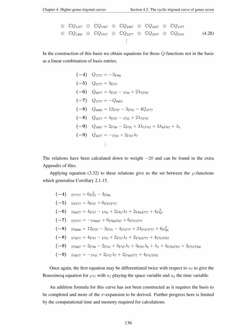
Chapter 4: Higher genus trigonal curves Section 4.2: The cyclic trigonal curve of genus seven
⊕ CQ1477 ⊕ CQ1567 ⊕ CQ2367 ⊕ CQ2457 ⊕ CQ1377
⊕ CQ1466 ⊕ CQ1557 ⊕ CQ2277 ⊕ CQ2357 ⊕ CQ2555
...
(4.28)
In the construction of this basis we obtain equations for those Q-functions not in the basis
as a linear combination of basis entries.
(−4) Q7777 = −3℘66
(−5) Q6777 = 3℘57
(−6) Q6677 = 4℘47 − ℘56 + 2λ7℘67
(−7) Q5777 = −Q6667
(−8) Q6666 = 12℘37 − 3℘55 − 4Q4777
(−8) Q5677 = 4℘37 − ℘55 + 2λ7℘57
(−9) Q5667 = 2℘36 − 2℘45 + 3λ7℘47 + 3λ6℘67 + λ5
(−9) Q4677 = −℘45 + 2℘47λ7
...
The relations have been calculated down to weight −20 and can be found in the extra
Appendix of files.
Applying equation (3.32) to these relations give us the set between the ℘-functions
which generalise Corollary 2.1.15.
(−4) ℘7777 = 6℘277 − 3℘66
(−5) ℘6777 = 3℘57 + 6℘67℘77
(−6) ℘6677 = 4℘47 − ℘56 + 2℘67λ7 + 2℘66℘77 + 4℘267
(−7) ℘5777 = −℘6667 + 6℘66℘67 + 6℘57℘77
(−8) ℘6666 = 12℘37 − 3℘55 − 4℘4777 + 24℘47℘77 + 6℘266
(−8) ℘5677 = 4℘37 − ℘55 + 2℘57λ7 + 2℘56℘77 + 4℘57℘67
(−9) ℘5667 = 2℘36 − 2℘45 + 3℘47λ7 + 3℘67λ6 + λ5 + 4℘56℘67 + 2℘57℘66
(−9) ℘4677 = −℘45 + 2℘47λ7 + 2℘46℘77 + 4℘47℘67
Once again, the first equation may be differentiated twice with respect to u7 to give the
Boussinesq equation for ℘77 with u7 playing the space variable and u6 the time variable.
An addition formula for this curve has not been constructed as it requires the basis to
be completed and more of the σ-expansion to be derived. Further progress here is limited
by the computational time and memory required for calculations.
136

Chapter 5
New approaches for Abelian functionsassociated to trigonal curves
In this chapter we discuss some new approaches, inspired by the techniques developed in
the investigation of the cyclic (4,5)-curve in Chapter 3. The techniques presented here
will be valid for any (n, s)-curve and we have used them to generate new results for the
two canonical trigonal curves. These results will be presented in full with some additional
details for the higher genus curves included.
5.1 Introduction
Our main aim in this chapter is to generalise the classic differential equations for the Weier-
strass ℘-function, presented earlier in Theorem 2.1.14 and Corollary 2.1.15.
[℘′(u)]2 = 4℘(u)3 − g2℘(u)− g3.
℘′′(u) = 6℘(u)2 − 12g2.
In Corollary 3.5.6 we presented a generalisation of the second equation for the cyclic (4,5)-
curve. This was a set of partial differential equations that expressed 4-index ℘-functions
using a polynomial of ℘-functions. Such relations have also been presented for lower genus
generalisations. For example Baker derived equations (2.66) for the (2,5)-case, while [30]
and [11] contain relations for the general (3,4) and cyclic (3,5)-curves respectively.
Baker’s hyperelliptic generalisations expressed each of the different ℘ijkl using a poly-
nomial of 2-index ℘-functions with degree two. (This is the logical generalisation given
℘(u) is a 2-index ℘-function in the new notation and ℘′′(u) a 4-index ℘-function.) However,
the trigonal and tetragonal generalisations all contain at least one equation with multiple 4-
index ℘-functions which cannot be separated out.
137

Chapter 5: New approaches for Abelian functions Section 5.1: Introduction
We explain this by examining the method used in Chapter 3 to derive the relations for the
(4,5)-case. Here we attained them through the derivation of a basis for Γ(J,O(2Θ[g−1])
),
the space of Abelian functions with poles of order at most two. The 2-index ℘-functions
were not sufficient to construct the basis and so Q-functions were used as well. Hence
the relations that express the non-basis entries as linear combinations of basis entries had
multiple Q-functions in them, and so our generalisation had equations with multiple ℘ijkl.
Note that this problem still occurs if the relations are derived from alternative methods.
For example, in [30] the relation for ℘2222 also contained a ℘1333 term. Here the relations
were not constructed using the σ-expansion and the basis, but rather using the expansion of
the Kleinian formula and algebraic manipulation of the formulae. However, in the construc-
tion of the basis for Γ(J,O(2Θ[3])
), we find that either Q2222 or Q1333 must be included.
In [9] Baker considers a genus three hyperelliptic curve and defines a function
∆ = ℘12℘23 − ℘23℘22 + ℘213 − ℘11℘33.
Each of the terms in ∆ has poles of order four and in general this function will have poles
of order three. (This may be checked by substituting the ℘-functions for their definitions
in σ-derivatives.) However, Baker showed that in the special case of the (2,7)-curve ∆ has
poles of order two. Hence it may be used in the basis of Γ(J,O(2Θ[g−1])
)avoiding the need
for any Q-functions. This would ensure that independent relations for each of the 4-index
℘-functions may be derived.
A function similar to ∆, (quadratic in 2-index ℘-functions with poles of order two) does
not exist in any of the trigonal or tetragonal cases that have been tested. Hence, since the
method in Chapter 3 of using Q-functions can be used for any (n, s)-curve it is reasonable
to focus on this. Recall that in general the number of 2-index ℘-functions is
(g + r − 1)!
r!(g − 1)!,
while the dimension of Γ(J,O(2Θ[g−1])
)is 2g. This means that the dimension of the ba-
sis grows faster than the number of 2-index ℘-functions and so an increasing number of
Q-functions will be required. Hence the relations for 4-index ℘-functions will become
increasingly interrelated. A more appropriate definition for the generalisation of the sec-
ond elliptic differential equation may be to put emphasis on fundamental Abelian functions
(those with poles of order two) instead of the 2-index ℘-functions.
For example, we could instead look for a set of equations for all the second derivatives
of fundamental Abelian functions, in which they are expressed using a polynomial of fun-
damental Abelian functions of degree at most two. However, this would imply an infinite
set of equations since there are an infinite number of fundamental Abelian functions. (For
example, the n-index Q-functions for progressively higher n.)
138

Chapter 5: New approaches for Abelian functions Section 5.1: Introduction
The approach that we use instead is to find expressions for all the 4-index ℘-functions
using a polynomial of the fundamental Abelian functions with degree two.
Definition 5.1.1. We will define a generalisation of the second elliptic differential equa-tion, (Corollary 2.1.15) as a set of equations that express all the 4-index ℘-functions using
a polynomial of degree two in those fundamental Abelian functions that give a basis of the
space Γ(J,O(2Θ[g−1])
).
Hence we will not substitute those Q-functions in the basis for their definition in ℘-
functions, but rather to treat them as extra 2-index ℘-functions. We can easily extract the
desired generalisation from the existing equations that have been derived by substituting
those 4-index ℘-functions that share their indices with basisQ-functions for these functions.
Using equation (3.32),
℘ijk` = −Qijk` + 2℘ij℘k` + 2℘ik℘j` + 2℘i`℘jk.
This also trivially gives us the equations in the generalisation that express the 4-index ℘-
functions with these indices. In Appendix C.3 we have presented the full generalisation, as
defined in Definition 5.1.1, for the cyclic (4,5)-curve. This contains relations for all 126 of
the 4-index ℘-functions from ℘6666 to ℘1111.
Note that we may now achieve the generalisation given in Definition 5.1.1 for any (n, s)-
curve using the methods set out in Chapter 3.
The next aim will be to find generalisations of the first elliptic differential equation,
[℘′(u)]2 = 4℘(u)3 − g2℘(u)− g3.
Definition 5.1.2. We will define a generalisation of the first elliptic differential equation,
(Theorem 2.1.14) as a set of equations for each of the possible products of two 3-index
℘-functions using a polynomial of fundamental Abelian function of degree at most three.
We often refer to such equations as quadratic 3-index relations, or just quadratic rela-tions for brevity.
In equation (2.65) we presented Baker’s generalisation of the first differential equation
for the functions associated to the (2,5)-curve, which matches Definition 5.1.2. In [30]
(Lemma 6.7) and [11] (Proposition 7.6) generalisations are presented for the general (3,4)
and cyclic (3,5)-curves. These contain 4-index ℘-functions with indices matching the Q-
functions in the basis, and when these are substituted back to Q-functions the relations
match Definition 5.1.2. However, both these sets of relations are incomplete, with the
lower weight relations missing. We aim to complete these sets in this chapter.
139

Chapter 5: New approaches for Abelian functions Section 5.1: Introduction
In Section 5.3.1 we discuss the methods that we use to derive the quadratic relations.
In the remainder of Section 5.3 we present generalisations for the specific cases. The most
efficient methods relies on the following set of equations associated with (n, s)-curves.
Definition 5.1.3. We define the bilinear relations associated with an (n, s)-curve as the set
of equations that are bilinear in the 2 and 3-index ℘-functions.
These do not exist in the elliptic case but have been found in the lower genus generali-
sations. For example, in [11] the authors derived the following relations for the ℘-functions
associated to the cyclic (3,5)-curve.
℘333 = 2℘44℘344 − 2℘34℘444 − ℘244
℘234 = 12℘34℘344 − ℘334℘44 + 1
2℘33℘444 + 1
2λ4℘344
℘233 = −℘33℘344 − 32℘444℘24 + 1
2℘334℘34 + 3
2℘244℘44 + 1
2λ4℘334 + 1
2℘333℘44
℘144 = −12℘334℘33 + 1
2℘333℘34 + ℘344℘24 − 1
2℘34℘244
℘134 = ℘234℘34 − ℘24℘334 + 12℘33℘244 − 1
2℘344℘23
℘133 = 12℘333℘24 − ℘33℘234 − 1
2℘23℘334 + ℘34℘233 − 3℘444℘14 + 3℘144℘44
℘124 = −℘134℘44 − 12℘144℘34 + ℘14℘344 + 1
2℘13℘444 + 1
2λ4℘144
℘134℘34 = −12℘33℘144 + 1
2℘344℘13 + ℘334℘14
℘114 = −12℘144℘23 − ℘134℘24 + ℘234℘14 + 1
2℘244℘13
℘111 = 23℘22℘123 + 1
3℘23℘122 + λ3℘114 − λ1℘144 − 1
3℘13℘222 − 2
3℘223℘12
− 23λ2℘124 + 1
3λ1℘224 + λ0℘244 + 1
3λ4℘112 (5.1)
These were derived directly from the set of relations that generalises the second ellip-
tic differential equation by using cross-differentiation on selected pairs from the set. For
example, substituting the relations for ℘4444 and ℘3444 into
∂
∂u3
(℘4444
)− ∂
∂u4
(℘3444
)= 0
would result in the first relation of (5.1). The same technique was used to derive the relations
in Proposition 3.5.7 for the (4,5)-case.
We note the following problems with this approach to the derivation of the bilinear
relations.
• It is not possible to know for sure if all such bilinear relations have been calculated.
• It is not known if the relations are given in the simplest form. (For example, it may
be possible to separate the relations to give two independent equations.)
• Using the approach on higher genus cases can become quite complicated. This is be-
cause the higher genus curve require more Q-functions in the basis for(J,O(2Θ[k])
)140

Chapter 5: New approaches for Abelian functions Section 5.1: Introduction
and hence there are more 4-index ℘-functions in each relation. Then the cross differ-
entiation approach may require triplets or quadruplets instead of pairs of equations
for example.
It becomes more difficult to derive the equations and to ensure all the bilinear rela-
tions are found.
In Section 5.2 of this chapter we present a new method to derive the full set of bilinear
relations associated to an (n, s) curve. This method employs the σ-function expansion at the
origin, discussed throughout this document and derived for the (4,5)-curve in Section 3.4.
While interesting on their own merit, these bilinear relations are motivated by their use
in the computationally efficient method to derive the quadratic 3-index relations, which is
discussed in Section 5.3. We also develop another method to find quadratic equations using
pole cancellations and the σ-expansion, for use once the efficient method is exhausted.
Throughout these two sections we present the full results of the calculations for the
cyclic (3,4) and (3,5)-cases, giving also some details for the higher genus curves. Finally in
Section 5.4 we consider the problem of constructing a basis for(J,O(3Θ[3])
)in the (3,5)-
case. This problem was solved in [30] for the (3,4)-curve but the corresponding results for
the (3,5)-case has yet to be considered. In Section 5.4 we use ideas from the previous two
sections to identify elements in this basis.
141

Chapter 5: New approaches for Abelian functions Section 5.2: Bilinear relations and B-functions
5.2 Bilinear relations andB-functions
In this section we introduce a new set of odd functions that belong to Γ(J,O(3Θ[g−1])
)— the space of Abelian functions associated to an (n, s)-curve with poles of order at most
three. The new functions may be expressed as a sum of products of 2-index and 3-index
℘-functions in which the poles of order five and four cancel.
We use the new functions, along with the 3-index ℘-functions to construct the odd part
of the basis for Γ(J,O(3Θ[g−1])
). Those functions that are not in the basis are expressed as
a linear combination of basis entries, which generate the bilinear relations discussed in the
introduction above.
The new functions were constructed to aid with the derivation of bilinear relations, how-
ever they may also be used in other areas of the theory where a basis for Γ(J,O(3Θ[g−1])
)is required.
5.2.1 Defining theB-functions
Consider a 2-index ℘-function multiplied by a 3-index ℘-function. This has poles of order
five when σ(u) = 0. We seek to find the combinations of such products that cancel higher
order poles. We do this using the definition of the functions as σ-derivatives and so these
calculations are valid for functions associated to any (n, s)-curve. We start by forming the
polynomial P(u) of all the possible combinations, (assuming five distinct indices).
P(u) =[c1℘ij℘klm + c2℘ik℘jlm + c3℘il℘jkm + c4℘im℘jkl + c5℘jk℘ilm (5.2)
+ c6℘jl℘ikm + c7℘jm℘ikl + c8℘kl℘ijm + c9℘km℘ijl + c10℘lm℘ijk](u),
for constants c1, . . . c10. We then substitute in the definition of the ℘-functions to obtain an
expression involving σ-derivatives. For example,
℘ij(u)℘klm(u) =σij(u)σklm(u)
σ(u)2− σi(u)σj(u)σklm(u)
σ(u)3
− σij(u)σlm(u)σk(u)
σ(u)3− σij(u)σkm(u)σl(u)
σ(u)3− σij(u)σkl(u)σm(u)
σ(u)3
+2σij(u)σk(u)σl(u)σm(u)
σ(u)4+σi(u)σj(u)σk(u)σlm(u)
σ(u)4
+σi(u)σj(u)σl(u)σkm(u)
σ(u)4+σi(u)σj(u)σm(u)σkl(u)
σ(u)4
− 2σi(u)σj(u)σk(u)σl(u)σm(u)
σ(u)5(5.3)
So P(u) is a sum of rational functions of σ-derivatives, with the denominators all σ(u)k
where k = 2, 3, 4 or 5. Each of the 10 original products contributes 10 fractions, as in
equation (5.3). Therefore P(u) has 100 terms in total — 10 with poles of order five, 40
142

Chapter 5: New approaches for Abelian functions Section 5.2: Bilinear relations and B-functions
with poles of order four, 40 with poles of order three and 10 with poles of order two.
We identify the numerator of those parts of the sum with denominator σ(u)k byNk(u).
P(u) =N5(u)
σ(u)5+N4(u)
σ(u)4+N3(u)
σ(u)3+N2(u)
σ(u)2.
We start by considering the parts which contribute to the poles of highest order. We find
this can be factored simply to give
N5(u) = −2σi(u)σj(u)σk(u)σl(u)σm(u)[c1 + c2 + · · ·+ c10
].
Hence only one condition of the coefficients is required to ensure the poles do not have
order five.
c1 + c2 + c3 + c4 + c5 + c6 + c7 + c8 + c9 + c10 = 0.
However, we find that the other parts do not factor as simply. We write a Maple procedure
to collect the parts together into terms with the same σ-derivatives. We find
N4(u) =[c1 + c3 + c6 + 2c9
]σi(u)σj(u)σkm(u)σl(u)
+[c2 + c3 + c8 + 2c7
]σi(u)σk(u)σjm(u)σl(u)
+[c2 + c4 + c9 + 2c6
]σi(u)σk(u)σjl(u)σm(u)
+[c1 + c2 + c5 + 2c10
]σi(u)σj(u)σk(u)σlm(u)
+[c1 + c4 + c7 + 2c8
]σi(u)σj(u)σkl(u)σm(u)
+[c3 + c4 + c10 + 2c5
]σi(u)σl(u)σjk(u)σm(u)
+[c5 + c7 + c9 + 2c3
]σil(u)σj(u)σk(u)σm(u)
+[c5 + c6 + c8 + 2c4
]σim(u)σj(u)σk(u)σl(u)
+[c6 + c7 + c10 + 2c2
]σik(u)σj(u)σl(u)σm(u)
+[c8 + c9 + c10 + 2c1
]σij(u)σk(u)σl(u)σm(u),
and hence we have a further 10 conditions of the constants, necessary to ensure P(u) has
poles of order at most three. We find that all 11 of the conditions may be satisfied if
c1 = 2c4 + 3c5 − c2 + 2c3, c8 = −2c5 − c3 + c2 − 2c4,
c6 = c3 + c5 − c2, c9 = −2c5 − c4 + c2 − 2c3,
c7 = c4 + c5 − c2, c10 = −c3 − c4 − 2c5,
(5.4)
where c2, c3, c4, c5 may take any value.
If we repeat this process on N3(u) we see that the 40 terms may be collected into 20
terms with each coefficient involving two of the constants. Hence we have a further 20
conditions to be satisfied if P(u) is to have poles of order at most two. We find that the
143

Chapter 5: New approaches for Abelian functions Section 5.2: Bilinear relations and B-functions
only simultaneous solution to these 20 conditions is to have all constants set to zero. Hence
it is not possible to remove from P(u) the terms contributing poles of order three and leave
a non-zero function.
However, we do have a non-zero solution in equation (5.4), that restricts P(u) to poles
of order at most three. There are four free parameters so we find that this may be separated
to give four different solutions. (To achieve this we let each of the free parameters be one
in turn, setting the others to zero.) Substituting these four solutions into equation (5.2)
identifies the four independent combinations that have poles of order at most three. We
define these combinations to be the B-functions.
Definition 5.2.1. Define the fourB-functions as follows.
BAijklm = ℘ij℘klm + 1
3℘jk℘ilm + 1
3℘jl℘ikm + 1
3℘jm℘ikl − 2
3℘kl℘ijm
− 23℘km℘ijl − 2
3℘lm℘ijk.
BBijklm = ℘ik℘jlm + 1
3℘jk℘ilm − 2
3℘jl℘ikm − 2
3℘jm℘ikl + 1
3℘kl℘ijm
+ 13℘km℘ijl − 2
3℘lm℘ijk.
BCijklm = ℘il℘jkm − 2
3℘jk℘ilm + 1
3℘jl℘ikm − 2
3℘jm℘ikl + 1
3℘kl℘ijm
− 23℘km℘ijl + 1
3℘lm℘ijk.
BDijklm = ℘im℘jkl − 2
3℘jk℘ilm − 2
3℘jl℘ikm + 1
3℘jm℘ikl − 2
3℘kl℘ijm
+ 13℘km℘ijl + 1
3℘lm℘ijk. (5.5)
Note that this derivation and definition is for functions associated to an arbitrary (n, s)
curve and not specific to the cyclic case. (The Maple worksheet in which the derivation was
conducted can be found in the extra Appendix of files.)
Remark 5.2.2.
(i) The B-functions are defined as a sum of Abelian functions and hence are Abelian
functions themselves. From the derivation above we know they have poles of order at
most three and hence belong to the vector space Γ(J,O(3Θ[g−1])
).
(ii) By Lemma 2.2.32 the 2-index ℘-functions are even with respect to the change of
variables u → [−1]u while the 3-index ℘-functions are odd. Hence the B-functions
are all odd functions since each term is the product of an odd and even function.
Remark 5.2.3. When the indices are not distinct the B-functions specify to simpler formu-
lae. In particular, if the indices are all equal then all four B-functions are zero.
BAiiiii = BB
iiiii = BCiiiii = BD
iiiii = 0.
Hence, no B-functions exist in the genus one case, which is related to the fact that there are
no bilinear relations associated with the elliptic curve.
144

Chapter 5: New approaches for Abelian functions Section 5.2: Bilinear relations and B-functions
Note also that when the indices are specified the B-functions often equal each other, or
are linearly dependent on each other. For example,
BAiiiij = BB
iiiij = BCiiiij = ℘ii℘iij − ℘ij℘iii.
BDiiiij = 2℘ij℘iii − 2℘ii℘iij = −2BA
iiiij.
5.2.2 Deriving bilinear relations
We will derive bilinear relations systematically through the construction of a basis for the
odd functions in Γ(J,O(3Θ[g−1])
). This mimics the derivation of the relations between Q-
functions in Lemma 3.5.5 through the construction of the basis Γ(J,O(2Θ[g−1])
)in Theo-
rem 3.5.3.
Recall that the space Γ(J,O(3Θ[g−1])
)will have dimension 3g by the Riemann-Roch
theorem. We may assign to this basis the 2g elements already identified in Γ(J,O(2Θ[g−1])
)and then search for the remaining elements amongst those functions with poles of order
three.
We start by including all the 3-index ℘-functions and then search systematically among
the B-functions at decreasing weight levels using techniques similar to those discussed
in Section 3.5. Since these functions are odd we may ignore the elements in the smaller
basis when constructing the linear polynomials, (since these were all even). We identify
those elements to add to the basis and obtain expressions for the non-basis entries as linear
combinations of basis entries. Substituting for the B-functions in these will leave us with
bilinear relations.
We use the following method, described for weight level −k, and implemented with
Maple.
1. Start by forming a sum of existing odd basis entries, each multiplied by an unde-
termined constant coefficient, ci. (These will be the 3-index ℘-functions and B-
functions of a higher weight). Include only those which may be combined with an
appropriate λ-monomial to give weight −k overall. (Note that all the possible ele-
ments of a higher weight have already been determined since we are working sys-
tematically in decreasing weights.)
From a simple extension of Lemma 3.5.2 we need not consider basis entries multi-
plied by rational functions in the λ. We also do not need to consider any constant
term since this would not be odd.
2. Add to this sum the B-functions of weight −k, each multiplied by an undetermined
constant coefficient, qi. (Note that often the different B-functions may be equal or
linearly dependent when the indices have been specified specified. If this is the case
then we need only include a minimal set of them.)
145

Chapter 5: New approaches for Abelian functions Section 5.2: Bilinear relations and B-functions
3. Substitute the functions for their definitions as σ-derivatives. This will give a sum of
rational functions which may be factored to leave σ(u)3 on the denominator. Take
the numerator, which should be a sum of products of triplets of σ-derivatives.
4. Substitute σ(u) in this sum for the σ-expansion at the origin. Note that the sum
contains λ-monomials with weight no lower than −k. Hence we may truncate the σ-
expansion after the polynomial which contains λ-monomials of weight−k. Evaluate
the σ-derivatives as derivatives of this expansion.
5. Expand the products to obtain a polynomial. Note that this will create terms with λ-
monomials of a lower weight than−k. These terms must be discarded since we would
not have all such terms with this λ-monomial, (because we truncated the expansion).
Hence any information gained from them would be invalid.
6. Collect this polynomial into a sum of the various uλ-monomials with coefficients
in the unknown constants ci, qi. Note that these coefficients will be linear in the
unknowns, (since the unknowns were from the original sum, not the expansions that
were multiplied).
7. Consider these coefficients as a series of linear equations in the unknowns that must
equal zero. Since it is linear it is relatively simple for a computer algebra package
like Maple to solve.
• If there is a unique solution for the ci in terms of the qi then each of the functions
at weight−k may be expressed as a linear combination of existing basis entries.
(To obtain the relations repeatedly set one of the qi to one and the others to zero
in the solution that was obtained.)
• However, it will more often be the case that this is not possible, and hence some
of the functions must be selected as basis entries.
Suppose that there are x unknowns and (x − y) of the unknowns may be ex-
pressed using the other y. This means that specifying y of the qi determines
numerical values for all the ci and the other qi. Hence y of the functions may
be expressed as a linear combination of basis entries and the others, which are
added to the basis.
To obtain the relations for the non-basis functions repeatedly set one of the
corresponding qi to one and the others to zero in the solution that was obtained.
Hence we have identified the basis entries at weight −k and obtained relations for
all the non-basis entries as a linear combination of basis entries. Substituting the
B-functions for their definitions into these will produce the bilinear relations.
146

Chapter 5: New approaches for Abelian functions Section 5.2: Bilinear relations and B-functions
Example 5.2.4 below demonstrates the use of this procedure. We follow it at succes-
sively lower weights, constructing the basis and equations as we proceed. Note that as the
weight decreases, both the the possible number of terms in the original sum and the size of
the σ-expansion increase. Hence the computations take more time and memory. The most
computationally intensive part is Step 5 where the triplets of expansions must be calculated
and the terms with weight in λ lower than −k discarded.
• Since all the terms in the end polynomial contain an unknown, we should not use the
new procedure described in Section 3.4. However, we can implement a procedure
similar to the one discussed in Section 3.6 for the addition formula.
This procedure only multiplies those terms that will not be discarded. To achieve this
we categorise the terms in the three expansions by their weights, and only consider
the combinations of three entries that result in an acceptable λ-weight.
• To further save computation time and memory distributed computing may be em-
ployed to expand the triplets of products in parallel.
5.2.3 The cyclic (3,4)-case
We have derived a complete set of bilinear relations for the cyclic (3,4)-case. We start
by giving an example of the procedure above by discussing the steps taken when the first
weight level was examined.
Example 5.2.4. The B-functions have five indices and when these are all the same the
functions reduce to zero. Hence in the (3,4)-case the lowest weight functions will be at
weight −6 with indices 2, 3, 3, 3, 3.Start by constructing the sum of existing basis entries. The entries at weight −6 are
℘222 and λ3℘333, (since we do not consider the even or constant functions).
We additionally add the B-functions at weight −6, multiplied by an unknown constant.
Since they are all linearly dependent we include only BA23333. We are left with the equation
0 = c1℘222 + c2λ3℘333 + q1BA23333.
We substitute the Abelian functions for σ-derivatives and take the numerator.
0 = c1
(3σ22σ2σ − σ222σ
2 − 2σ32
)+ λ3c2
(3σ33σ3σ − σ333σ
2 − 2σ33
)+ q1
(σ23σσ333 − σ23σ33σ3 − σ2σ3σ333 − σ33σσ233 + σ2
33σ2 + σ23σ233
).
We then substitute in the σ-expansion truncated afterC11, since this was the first polynomial
to contain λ3. Expanding the products of expansions will generate terms with λ23 and λ2
3
which must be discarded.
147

Chapter 5: New approaches for Abelian functions Section 5.2: Bilinear relations and B-functions
The polynomial that is left is collected into uλ-monomials with coefficients in the un-
knowns. Setting these to zero we see that there is a solution for any value of q1. Setting
q1 = 1 we find
BA23333 = −1
2℘222 − 1
2λ3℘333.
Hence no B-functions at weight −6 need to be added to the basis. Substituting for the
B-function using equation (5.5) we have
0 = ℘222 + λ3℘333 + 2℘23℘333 − 2℘33℘233,
which is the first of the bilinear relations associated with this curve.
Following this procedure at successively lower weights allows us to examine all the B-
functions. We find that three need to be included in the basis, one each at weight −9, −10
and −13. We choose BA13333, BB
12333 and BA11333 respectively. Then all the other B-functions
may be expressed as a linear combination of these and the ℘ijk. (The Maple worksheet in
which these calculations are performed can be found in the extra Appendix of files.) We
obtain the following set of relations.
(−6) BA23333 = −1
2℘222 − 1
2λ3℘333
(−7) BA22333 = −2℘133
(−8) BA22233 = 4
3℘123
(−9) BA22223 = −2℘122 + 1
2λ3℘222 + 1
2λ3
2℘333 − 2λ2℘333 − 4BA13333
(−10) BA12333 = −2BB
12333
(−11) BA12233 = 4
3℘113
(−11) BC12233 = 1
3℘113
(−12) BA12223 = −λ1℘333 − λ3B
A13333
(−12) BD12223 = ℘112 + 2λ1℘333 + 2λ3B
A13333
(−13) BA12222 = 2
3λ2℘133 − 1
3λ1℘233 − 4
3BA
11333 − λ3BC12333
(−14) BA11233 = 3
2λ3℘113 − λ2℘123 + 1
2λ1℘223
(−14) BC11233 = 0
(−15) BA11223 = 3
2λ3℘112 − λ2℘122 − ℘111 + 1
3λ1℘222 − 1
6λ3λ1℘333
− 43λ0℘333 − 2
3λ2B
A13333
(−15) BB11223 = −1
6λ1℘222 − 1
6λ3λ1℘333 − 4
3λ0℘333 − 2
3λ2B
A13333
(−16) BA11222 = 3λ1℘133 − 4λ0℘233 −BA
11333λ3 − 2λ2BB12333
(−17) BA11133 = 2
3λ2℘113 − 4
3λ1℘123 + 2λ0℘223
148

Chapter 5: New approaches for Abelian functions Section 5.2: Bilinear relations and B-functions
(−18) BA11123 = −λ3λ0℘333 + λ0℘222 + 2
3λ2℘112 − 4
3λ1℘122 − λ1B
A13333
(−18) BC11123 = −λ3λ0℘333 − 2λ0℘222 − 1
3λ2℘112 + 2
3λ1℘122 − λ1B
A13333
(−19) BA11122 = 8
3λ0℘133 − 4
9λ2
2℘133 + 29λ2λ1℘233 + 4
3λ3λ1℘133 − 2λ3λ0℘233
− 2BB12333λ1 − 4
9λ2B
A11333
(−21) BA11113 = −2λ2λ0℘333 − 3λ0℘122 + 1
2λ1
2℘333 + 12λ1℘112 − 4λ0B
A13333
(−22) BA11112 = −1
3λ2λ1℘133 + 2
3λ1
2℘233 + 3λ3λ0℘133 − 2λ2λ0℘233
− 4λ0BB12333 − 1
3λ1B
A11333 (5.6)
These calculations required the σ-function expansion up to C26. We can now make the
following statement.
Theorem 5.2.5. Every bilinear relation associated to the cyclic (3,4)-curve may be given
as a linear combination of the set below.
(−6) 0 = ℘222 + λ3℘333 + 2℘23℘333 − 2℘33℘233
(−7) 0 = 2℘133 + ℘22℘333 + ℘23℘233 − 2℘33℘223
(−8) 0 = −4℘123 + 4℘22℘233 − 2℘23℘223 − 2℘33℘222
(−9) 0 = 4℘122 − λ3℘222 − λ32℘333 + 4λ2℘333 − 2℘23℘222 + 2℘22℘223
+ 8℘13℘333 − 8℘33℘133
(−10) 0 = −℘12℘333 + ℘23℘133 + 2℘33℘123 − 2℘13℘233
(−11) 0 = 4℘113 − 3℘12℘233 − ℘22℘133 + 2℘23℘123 + 2℘33℘122
(−11) 0 = ℘113 − 3℘13℘223 + 2℘22℘133 + 2℘23℘123 − ℘33℘122
(−12) 0 = λ3
(℘13℘333 − ℘33℘133
)+ λ1℘333 + ℘12℘223 − ℘23℘122
(−12) 0 = ℘13℘222 − ℘112 − 2λ3
(℘13℘333 − ℘33℘133
)− 2λ1℘333
− 2℘22℘123 + ℘23℘122
(−13) 0 = 3λ3
(℘13℘233 − ℘23℘133
)− 2λ2℘133 + λ1℘233 + 3℘12℘222
− 3℘22℘122 + 4℘11℘333 + 4℘13℘133 − 8℘33℘113
(−14) 0 = −4℘12℘133 + 4℘13℘123 − 2℘23℘113 + 2℘33℘112
(−14) 0 = 92λ3℘113 − 3λ2℘123 + 3
2λ1℘223 − 3℘11℘233 − ℘12℘133 − 2℘13℘123
+ 4℘23℘113 + 2℘33℘112
(−15) 0 = −℘11℘223 − 23℘12℘123 − 1
3℘13℘122 + 2
3℘22℘113 + 4
3℘23℘112
+ 32λ3℘112 − 2
3λ2
(℘13℘333 − ℘33℘133
)− λ2℘122 − ℘111
+ 13λ1℘222 − 1
6λ3λ1℘333 − 4
3λ0℘333
149

Chapter 5: New approaches for Abelian functions Section 5.2: Bilinear relations and B-functions
(−15) 0 = −23℘12℘123 + 2
3℘13℘122 − 1
3℘22℘113 + 1
3℘23℘112
− 23λ2
(℘13℘333 − ℘33℘133
)− 1
6λ1℘222 − 1
6λ3λ1℘333 − 4
3λ0℘333
(−16) 0 = −λ3
(℘11℘333 + ℘13℘133 − 2℘33℘113
)− 2λ2
(℘13℘233 − ℘23℘133
)+ 3λ1℘133 − 4λ0℘233 − ℘11℘222 − ℘12℘122 + 2℘22℘112
(−17) 0 = 23λ2℘113 − 4
3λ1℘123 + 2λ0℘223 − 4
3℘11℘133 + 2
3℘13℘113 + 2
3℘33℘111
(−18) 0 = −λ3λ0℘333 + λ0℘222 + 23λ2℘112 − 4
3℘11℘123 + 1
3℘12℘113
+ 13℘13℘112 + 2
3℘23℘111 − 4
3λ1℘122 − λ1
(℘13℘333 − ℘33℘133
)(−18) 0 = −λ3λ0℘333 − 2λ0℘222 − 1
3λ2℘112 − 5
3℘12℘113 + 2
3℘11℘123
+ 43℘13℘112 − 1
3℘23℘111 + 2
3λ1℘122 − λ1
(℘13℘333 − ℘33℘133
)(−19) 0 = 8
3λ0℘133 − 4
9λ2
2℘133 − 2λ1
(℘13℘233 − ℘23℘133
)− 4
9λ2
(℘11℘333 + ℘13℘133 − 2℘33℘113
)+ 2
9λ2λ1℘233
+ 43λ3λ1℘133 − 2λ3λ0℘233 − 4
3℘11℘122 + 2
3℘12℘112 + 2
3℘22℘111
(−21) 0 = −2λ2λ0℘333 − 3λ0℘122 − 4λ0
(℘13℘333 − ℘33℘133
)+ 1
2λ1
2℘333
+ 12λ1℘112 + ℘13℘111 − ℘11℘113
(−22) 0 = −13λ2λ1℘133 − ℘11℘112 + ℘12℘111 − 4λ0
(℘13℘233 − ℘23℘133
)− 1
3λ1
(℘11℘333 + ℘13℘133 − 2℘33℘113
)+ 2
3λ1
2℘233
+ 3λ3λ0℘133 − 2λ2λ0℘233
Proof. First we note that these identities are derived simply from equations (5.6) by substi-
tuting for the definition of the B-functions.
Now, consider a relation that is bilinear in 2 and 3-index ℘-functions. Due to the parity
properties of the ℘-functions we know that the relations must be odd or even. If the relation
were even then it could not contain any ℘ijk and so would only be trivially bilinear. Hence
the relations we consider are odd, and therefore cannot contain a constant term or terms
with a single 2-index ℘-function. Each term must either be a constant multiplied by a ℘ijkor a constant multiplied by a ℘ij℘ijk.
Further, the terms with ℘ij℘ijk must together cancel the poles of order four and five,
since ℘ijk has only poles of order three. We have established that all such combinations are
given by B-functions as defined in Definition 5.2.1.
Next we note that due to the results of Section 3.3 all such relations must be homoge-
neous in the Sato weights. Now, in the derivation of the basis described above we found all
the relations between the ℘ijk and B-functions at each weight, (up to linear dependence).
150

Chapter 5: New approaches for Abelian functions Section 5.2: Bilinear relations and B-functions
The relations in the theorem were derived from these by substituting the B-functions
for their definitions. (Note that we exclude relations for those B-functions that are linearly
dependent on the ones used, since these would have resulted in linearly dependent bilinear
relations.) Hence the set presented above is sufficient to generate all such relations.
Remark 5.2.6.
(i) In Lemma 6.5 of [30] bilinear relations associated to the general (3,4)-curve are pre-
sented. These were derived using the method of cross-differentiation discussed above.
If we make the following change of variables for the curve coefficients then we will
move from the general to the cyclic case.
µ1 = 0, µ4 = 0, µ2 = 0, µ5 = 0, µ8 = 0,
µ3 = λ3, µ6 = λ2, µ9 = λ9, µ12 = λ0.
Substituting these into the relations derived in [30] will transform them into relations
from Theorem 5.2.5. (Or a linear combination of the relations from Theorem 5.2.5.)
Note however, that not all the relations were present in [30] and this new method has
allowed the complete set to be derived.
(ii) In Lemma 8.1 of [30] a full basis for Γ(J,O(3Θ[2])
)was derived. The odd Abelian
functions included alongside the ℘ijk here were derivatives of Q-functions. These are
not identical toB-functions in general, however we note that the three entries selected
are at the same weights as the B-functions selected above, and so play the same role
in the basis.
5.2.4 The cyclic (3,5)-case
This calculation was repeated for the cyclic (3,5)-case. The following nineteenB-functions
were used as a basis at the weight levels indicated in brackets.
(−8) BB33344 (−16) BB
12334
(−9) BB23444 (−17) BB
12333, BC12244, B
A11444
(−11) BD23334, B
A22444 (−18) BB
11344
(−12) BB13444 (−19) BC
12233
(−13) BC13344 (−20) BD
12224, BB11244
(−14) BA22244, B
D13334, B
B12444 (−23) BA
11144
(−15) BC12344
(5.7)
At each weight level for which B-functions exist we obtained a set of relations express-
ing the linearly independent B-functions as a linear combination of basis entries. (This
required the σ-function expansion up to C38.)
151

Chapter 5: New approaches for Abelian functions Section 5.2: Bilinear relations and B-functions
(−6) BA34444 = −1
2℘244 − 1
2℘333
(−7) BA33444 = 2℘234 − λ4℘344
(−8) BA24444 = −2
3℘233 + 1
3λ4℘334 − 1
2BA
33344
(−9) BA33334 = −2℘144 +BB
23444
(−9) BA23444 = −2℘144 + 2℘224 − λ4℘244 − 2BB
23444
...
(−32) BA11112 = −2
7λ2λ1℘133 − 2λ2λ0℘233 + 5
7λ3λ0℘133 − 1
2λ4λ1
2℘334 + λ12℘233
− 121λ4
2λ2λ1℘334 − 17λ4λ3λ0℘233 − 6
7λ4
2λ3λ0℘334 + 142λ4λ2λ1℘233 + 3λ4λ2λ0℘334
+ 821λ4
4λ0℘334 − 67λ3
2λ0℘334 − 421λ4
3λ0℘233 + λ1λ0℘334 + 17λ3λ2λ1℘334
− 6λ0BC12244 +
(32λ3λ1 − 8λ4λ0
)BB
12444 + (6λ4λ0 − λ3λ1)BD13334
+(
314λ2λ1 + 2
7λ4
2λ0 − 97λ3λ0
)BD
23334 + 27λ4
2λ0℘133 + 12λ1B
D12224
+(
1514λ4λ3λ0 − 3
4λ1
2 + 114λ4λ2λ1 − 4
7λ4
3λ0
)BB
33344 + 2λ0BA11444
+(
114λ2λ1 − 4
7λ4
2λ0 − 37λ3λ0
)BA
22444 + 32λ4λ0B
A22244 − 3
4λ1B
B11244 (5.8)
The full list can be found in Appendix D.1 and the corresponding Maple worksheet in the
extra Appendix of files.
Theorem 5.2.7. Every bilinear relation associated to the cyclic (3,5)-curve may be given
as a linear combination of the set obtained from equations (5.8) by substituting for the
B-functions. The full list is available in the extra Appendix of files.
(−6) 0 = −12℘244 − 1
2℘333 − ℘34℘444 + ℘44℘344
(−7) 0 = 2℘234 − λ4℘344 − ℘33℘444 − ℘34℘344 + 2℘44℘334
(−8) 0 = 13λ4℘334 − 2
3℘233 − 2
3℘33℘344 + 1
3℘34℘334 + 1
3℘44℘333 − ℘24℘444 + ℘44℘244
(−9) 0 = −2℘144 − ℘33℘334 + ℘34℘333 + ℘24℘344 − ℘34℘244
(−9) 0 = 2℘224 − 2℘144 − λ4℘244 − ℘23℘444 + ℘34℘244 + 2℘44℘234 − 2℘24℘344
...
(−32) 0 = 17λ4λ3λ0℘233 − 15
14λ4λ3λ0
(43℘33℘344 − 2
3℘34℘334 − 2
3℘44℘333
)− 5
7λ3λ0℘133
+ λ3λ1
(℘14℘333 − 2℘33℘134 + ℘34℘133
)− 1
42λ4λ2λ1℘233 + 4
21λ3
4λ0℘233 − λ1λ0℘334
− 32λ4λ0
(43℘22℘244 − 2
3℘24℘224 − 2
3℘44℘222
)+ 8λ4λ0
(℘14℘244 − ℘24℘144
)− λ2
1℘233
− 114λ2λ1
(℘22℘444 + ℘24℘244 − 2℘44℘224
)− 6λ4λ0
(℘14℘333 − 2℘33℘134 + ℘34℘133
)− 3
14λ2λ1
(℘24℘333 − 2℘33℘234 + ℘34℘233
)− 3
2λ3λ1
(℘14℘244 − ℘24℘144
)+ ℘11℘112
− 27λ2
4λ0
(℘24℘333 − 2℘33℘234 + ℘34℘233
)+ 4
7λ2
4λ0
(℘22℘444 + ℘24℘244 − 2℘44℘224
)+ 6
7λ2
4λ3λ0℘334 − 114λ4λ2λ1
(43℘33℘344 − 2
3℘34℘334 − 2
3℘44℘333
)+ 6
7λ2
3λ0℘334 + . . .
152

Chapter 5: New approaches for Abelian functions Section 5.2: Bilinear relations and B-functions
· · ·+ 47λ3
4λ0
(43℘33℘344 − 2
3℘34℘334 − 2
3℘44℘333
)− 3λ4λ2λ0℘334 + 1
21λ2
4λ2λ1℘334
+ 97λ3λ0
(℘24℘333 − 2℘33℘234 + ℘34℘233
)+ 3
7λ3λ0
(℘22℘444 + ℘24℘244 − 2℘44℘224
)+ 3
4λ2
1
(43℘33℘344 − 2
3℘34℘334 − 2
3℘44℘333
)+ 1
2λ4λ
21℘334 − 8
21λ4
4λ0℘334 + 27λ2λ1℘133
− 12λ1
(℘14℘222 − 2℘22℘124 + ℘24℘122
)− 2λ0
(℘11℘444 + ℘14℘144 − 2℘44℘114
)+ 3
4λ1
(43℘12℘144 − 4
3℘14℘124 + 2
3℘24℘114 − 2
3℘44℘112
)+ 2λ2λ0℘233 − 2
7λ2
4λ0℘133
+ 6λ0
(℘14℘224 − 2
3℘22℘144 − 2
3℘24℘124 + 1
3℘44℘122
)− ℘12℘111 − 1
7λ3λ2λ1℘334
Proof. We follow the arguments in the proof of Theorem 5.2.5.
Remark 5.2.8. In Proposition 7.5 of [11] the authors presented a set of bilinear relations
associated to the cyclic (3,5)-curve that was recalled in equations (5.1) during the introduc-
tion to this chapter. These relations were derived using the method of cross-differentiation
of relations from Definition 5.1.1. We can see that the first four relations match ours, (dif-
fering by an overall multiplicative constant). However, note that the second relation at
weight −9 had not been picked up by the method of cross-differentiation. Additionally, the
new approach has found extra relations at some other weight levels considered in [11] and
relations at all the higher weights that were not considered.
In [11] the authors did not present a basis for Γ(J,O(3Θ[2])
). The B-functions we
have identified in (5.7) may be used but this will not be enough to complete the basis. We
consider this problem is Section 5.4.
5.2.5 Higher genus curves
The procedure has been applied to the cyclic (4,5)-curve down to weight −35, (which
uses the σ-expansion up to C47). The first few bilinear relations were presented earlier in
Proposition 3.5.7, with all the available relations in the extra Appendix of files. The lowest
weight relation will involve B11112 at weight −51 but these lower weight equations have
not been derived due to computational limitations.
The first few bilinear identities for the cyclic (3,7)-case are presented below.
(−6) 0 = −12℘466 − 1
2℘555 − 1
2λ6℘666 − ℘56℘666 + ℘66℘566
(−7) 0 = −2℘366 + 2℘456 − ℘55℘666 − ℘56℘566 + 2℘66℘556
(−8) 0 = 23℘356 − 2
3℘455 − 2
3℘55℘566 + 1
3℘56℘556 + 1
3℘66℘555 − ℘46℘666 + ℘66℘466
(−9) 0 = −2℘355 − 32λ6℘466 + 1
2λ6℘555 + 1
2λ2
6℘666 − 2λ5℘666
− ℘55℘556 + ℘56℘555 + ℘46℘566 − ℘56℘466 − 4℘36℘666 + 4℘66℘366
(−9) 0 = 2℘446 − ℘45℘666 + ℘56℘466 + 2℘66℘456 − 2℘46℘566
153

Chapter 5: New approaches for Abelian functions Section 5.3: Quadratic relations
5.3 Quadratic relations
In this section we aim to find generalisations of the classic differential equation for the
Weierstrass ℘-function,
[℘′(u)]2 = 4℘(u)3 − g2℘(u)− g3.
In Definition 5.1.2 we defined these as quadratic relations — a set of equations for each
of the possible products of two 3-index ℘-functions using a polynomial of fundamental
Abelian function of degree at most three.
We start by discussing the various methods used to obtain the relations and present a
procedure to use for any (n, s)-curve. We then discuss the results for specific cases includ-
ing the canonical trigonal curves.
5.3.1 Deriving quadratic relations
Deriving quadratic relations from bilinear relations
Consider the bilinear relations discussed in the previous section. An arbitrary relation will
be a sum of terms containing only a 3-index ℘-function, plus a sum of terms containing the
product of a 3-index and a 2-index ℘-function.
0 =∑i
(ci℘i1i2i3
)+∑j
(cj℘j1j2℘j3j4j5
). (5.9)
We can derive equations with quadratic terms in 3-index ℘-functions from the bilinear re-
lations using the following two methods.
• Differentiating the bilinear relations:
For example, differentiating equation (5.9) with respect to uk gives
0 =∑i
(ci℘i1i2i3k
)+∑j
(cj℘j1j2k℘j3j4j5 + ℘j1j2℘j3j4j5k
).
We then need to substitute for the 4-index ℘-functions using equations in Definition
5.1.1. Since these were of total degree two, the total degree of the equation we are
left with will be three. (Note that this method assumes the relations for the 4-index
℘-functions at this weight have already been derived. This may be achieved for any
(n, s)-curve using the methods of Chapter 3, as discussed in the introduction to this
Chapter.)
So this leaves us with a set of equations, each containing a sum of quadratic 3-index
terms and a degree three polynomial in the 2-index ℘-functions.
154

Chapter 5: New approaches for Abelian functions Section 5.3: Quadratic relations
• Multiply bilinear equations by a 3-index ℘-function:
For example, multiplying equation (5.9) by ℘klm gives
0 =∑i
(ci℘i1i2i3℘klm
)+∑j
(cj℘j1j2℘j3j4j5℘klm
).
Due to the results of Section 3.3 we know such an equation must have homogeneous
weight. Hence the weight of the quadratic 3-index terms that are multiplied by 2-
index ℘-functions are higher than those that are not. We will search for relations at
successively lower weights and so assume that the relations for these higher weight
quadratic terms are known. Substituting for these, we are left with a sum of quadratic
3-index terms and a polynomial in the 2-index ℘-functions of degree at most four.
Remark 5.3.1. Those equations derived from the second method with degree four terms
should be combined to eliminate these terms. If it is not possible to reduce them all them
we may discard some of the equations.
The degree four polynomials in the 2-index ℘-functions that are generated as a side
product are known as Kummer relations and may have geometric significant in another area
of the theory. We do not comment further, but note that it is an ongoing area of research.
Once we have found all the relations at a specific weight using these methods, we need
to manipulate the equations to find separate relations for each of the quadratic 3-index
terms. We achieve this by treating these terms as variables and solving simultaneously. If
there is enough relations then the generalisation can be completed at that weight. If not then
we should be able to express most of the quadratic 3-index terms as a polynomial involving
the others.
These two methods were developed in [30] for the functions associated to the (3,4)-
curve. At each weight level the methods were supplemented by relations obtained from
the expansion of the Kleinian formula, (see Section 3.2). As discussed elsewhere in this
document, the expansion of this formula does not yield useful relations for (n, s)-curves
with n > 4. Also, the sets of relations for the trigonal cases have yet to be completed using
only these approaches and it is questionable whether this is possible.
Deriving quadratic relations from the σ-expansion
An alternative way to derive quadratic 3-index relations would be to use the σ-function ex-
pansion about the origin which may be derived using the methods discussed in Section 3.4.
We can determine the possible terms in the expression for a particular quadratic 3-index
product as those which are of degree three or less in the fundamental Abelian functions and
have the correct weight. We then form the polynomial with unidentified constant coeffi-
cients, substitute in the σ-expansion and set the coefficients of the λu-monomials to zero
to determine the constants.
155

Chapter 5: New approaches for Abelian functions Section 5.3: Quadratic relations
Example 5.3.2. Consider ℘2333 associated to the cyclic (3,4)-curve. We will derive an ex-
pression for it using the σ-expansion. Start by considering the possible terms in the expres-
sion, which will be those of degree at most three and weight −6.
℘2333 = g1℘
333 + g2℘
223 + g3℘22℘33 + g4℘13 + g5λ3℘23 + g6λ
23 + g7λ2,
for some constants g1, . . . , g7. We substitute the ℘-functions for their definitions as σ-
derivatives and take the numerator to find
0 = −σ2333σ
4 + 6σ333σ3σ33σ3 − 4σ333σ
2σ33 − 9σ2
33σ23σ
2 + 12σ33σ43σ − 4σ6
3
+ g1(3σ233σ
23σ
2 − σ333σ
3 − 3σ33σ43σ + σ6
3) + g2(σ4σ223 − 2σ3σ23σ2σ3 + σ2σ2
2σ23)
+ g3(σ4σ22σ33 − σ3σ22σ23 − σ3σ2
2σ33 + σ2σ22σ
23) + g4(σ4σ1σ3 − σ5σ13)
+ g5(λ3σ4σ2σ3 − λ3σ
5σ23) + g6λ23σ
6 + g7λ2σ6. (5.10)
We then substitute in the σ-expansion truncated after C11, the first polynomial that con-
tains λ2. We expand the products and discard terms with lower weights in λ. Setting the
coefficients of the λu-monomials to zero we find
℘2333 = 4℘3
33 + 4℘13 + ℘223 − 4℘22℘33.
Since these relations have poles of order six this procedure involves the multiplication
of six large expansions. (See equation (5.10) which in which each term was a multiple of
six σ-derivatives.) This can be computationally difficult even at the high weights and is not
easily applicable for generating the complete set of relations.
Canceling the higher order poles
The process of deriving quadratic equations from the σ-expansion may be simplified by the
following result, valid for the ℘-functions associated to any (n, s)-curve.
Theorem 5.3.3. For arbitrary constants h1, h2, h3, h4, h5 the following polynomial has
poles of order four and no higher.
℘ijk℘lmn − (h1 + h2 + h3 + h4 + h5 − 2)℘in℘jl℘km
− (h4 + h5)℘ij℘kl℘mn + (h1 + h3 + h4 + h5 − 2)℘ij℘km℘ln
− (h1 + h3)℘ij℘kn℘lm + (h1 + h2 + h4 + h5 − 2)℘ik℘jl℘mn
− (h1 + h5)℘ik℘jm℘ln + (h1 + h2 + h3 + h4 − 2)℘in℘jk℘lm
− (h1 + h2)℘il℘jk℘mn + h1℘il℘jm℘kn + h2℘il℘jn℘km − (h3 + h4)℘im℘jk℘ln
+ h3℘im℘jl℘kn + h4℘im℘jn℘kl − (h2 + h4)℘ik℘jn℘lm + h5℘in℘jm℘kl.
156

Chapter 5: New approaches for Abelian functions Section 5.3: Quadratic relations
Proof. Substitute the ℘-functions for their definitions as σ-derivatives. Each term becomes
a sum of rational functions of σ-derivatives with the denominator σ(u)k for k ≤ 6. We
find that all those terms with k = 5, 6 cancel. Hence, since σ(u) is an entire function, the
polynomial has poles of order at most four, occurring when σ(u) = 0.
This result was constructed after noting the similarities in the cubic terms of the quadratic
equations already discovered. It was derived by considering the general sum of terms cubic
in the 2-index ℘-functions, with each term multiplied by an undetermined constant. Then
the constants were set to ensure the poles of order five and six canceled with those in
℘ijk℘lmn. (A similar approach to the construction of the B-functions in the last section.)
Note that there are no values of h1, . . . , h5 that cancel the poles of order four.
This same approach was used with additional terms in the polynomial to make the
following remarks.
Remark 5.3.4. We have considered ℘ijk℘klm added to increasing wider classes of poly-
nomials in an attempt to cancel poles using only the definition of the Abelian functions as
σ-derivatives.
1. Using a polynomial of ℘ij in which each term has degree three — the poles of order
five and six may be canceled. (This is Theorem 5.3.3 above.)
2. Include also terms in ℘ij with degree less than three — the poles of order five and six
may be canceled.
3. Include also linear terms in the 4-index Q-functions — the poles of order five and six
may be canceled.
4. Include also terms with a product of a 2-index ℘-function and a 4-index Q-function
— the poles of order four, five and six may be canceled.
5. Include also terms with a product of two 4-index Q-functions — the poles of order
four, five and six may be canceled.
(The Maple worksheet in which the cancellations were investigated is available in the
extra Appendix of files.)
Thus, when deriving quadratic 3-index relations using the σ-expansion, we may start
by identifying the cubic terms using Theorem 5.3.3. We then need to identify the correct
values of h1, . . . , h5 along with the coefficients of the degree two terms in the fundamental
Abelian functions.
This reduces the polynomial to one with poles of degree four, and so four expansions
must be multiplied instead of six. This is much easier computationally, but still far more
157
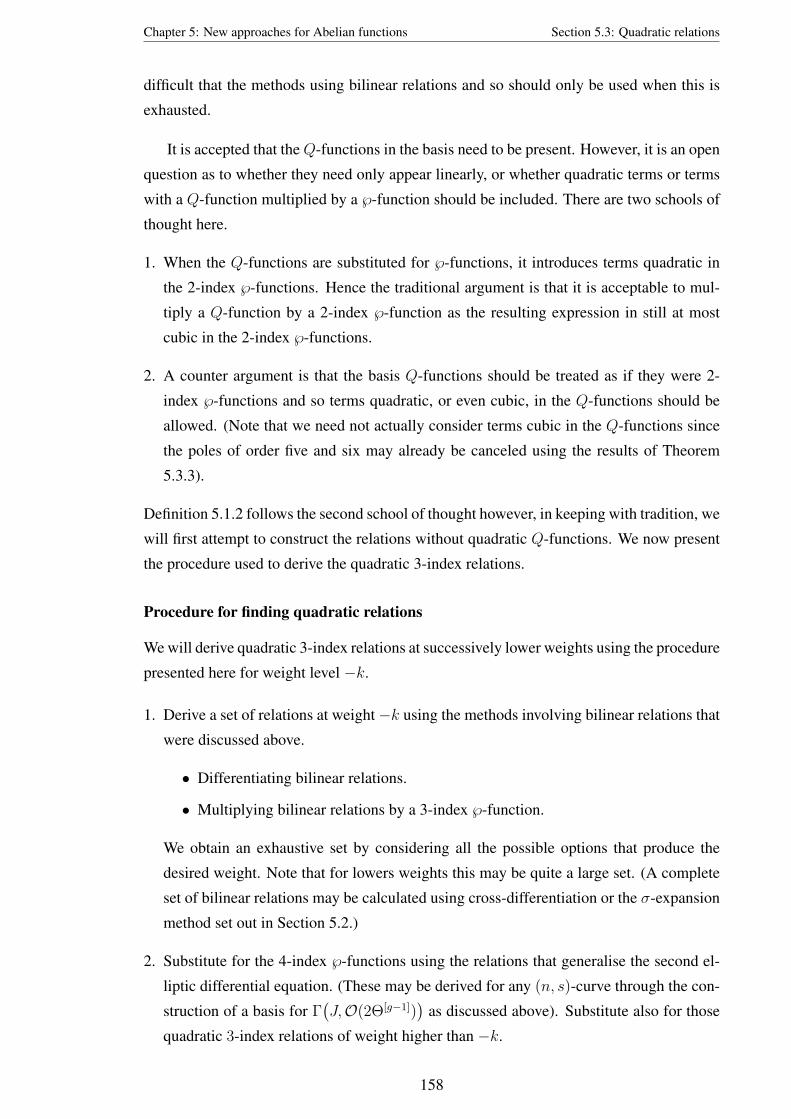
Chapter 5: New approaches for Abelian functions Section 5.3: Quadratic relations
difficult that the methods using bilinear relations and so should only be used when this is
exhausted.
It is accepted that theQ-functions in the basis need to be present. However, it is an open
question as to whether they need only appear linearly, or whether quadratic terms or terms
with a Q-function multiplied by a ℘-function should be included. There are two schools of
thought here.
1. When the Q-functions are substituted for ℘-functions, it introduces terms quadratic in
the 2-index ℘-functions. Hence the traditional argument is that it is acceptable to mul-
tiply a Q-function by a 2-index ℘-function as the resulting expression in still at most
cubic in the 2-index ℘-functions.
2. A counter argument is that the basis Q-functions should be treated as if they were 2-
index ℘-functions and so terms quadratic, or even cubic, in the Q-functions should be
allowed. (Note that we need not actually consider terms cubic in the Q-functions since
the poles of order five and six may already be canceled using the results of Theorem
5.3.3).
Definition 5.1.2 follows the second school of thought however, in keeping with tradition, we
will first attempt to construct the relations without quadratic Q-functions. We now present
the procedure used to derive the quadratic 3-index relations.
Procedure for finding quadratic relations
We will derive quadratic 3-index relations at successively lower weights using the procedure
presented here for weight level −k.
1. Derive a set of relations at weight−k using the methods involving bilinear relations that
were discussed above.
• Differentiating bilinear relations.
• Multiplying bilinear relations by a 3-index ℘-function.
We obtain an exhaustive set by considering all the possible options that produce the
desired weight. Note that for lowers weights this may be quite a large set. (A complete
set of bilinear relations may be calculated using cross-differentiation or the σ-expansion
method set out in Section 5.2.)
2. Substitute for the 4-index ℘-functions using the relations that generalise the second el-
liptic differential equation. (These may be derived for any (n, s)-curve through the con-
struction of a basis for Γ(J,O(2Θ[g−1])
)as discussed above). Substitute also for those
quadratic 3-index relations of weight higher than −k.
158

Chapter 5: New approaches for Abelian functions Section 5.3: Quadratic relations
3. There may be terms in 2-index ℘-functions with degree four. Eliminate these if possible
by treating them as variables and solving simultaneously. Discard any equations where
the terms of degree four cannot be eliminated.
4. Identify the quadratic 3-index terms as variables in the remaining set of equations and
solve simultaneously. If a solution can be found that expresses each quadratic 3-index
term as a polynomial in fundamental Abelian functions then we are finished. However,
it is often the case that several of the quadratic 3-index terms are used in the expressions
for the others.
5. Using the σ-expansion method, identify expressions for those quadratic 3-index terms
which are used to express the others.
(i) First use Theorem 5.3.3 to identify the cubic terms, (with unknown constants
h1, . . . , h5).
(ii) Then form the general quadratic polynomial of 2-index ℘-functions at this weight,
(with each term multiplied by an unknown constant). Add to this terms involving
the basis Q-functions that are either linear or multiplied by a 2-index ℘-function.
(Note that if we cannot find a solution in the next step we may return to this step
and also include terms which are a multiple of two Q-functions.)
(iii) Identify the unknown constants using the σ-expansion as normal — substitute
the Abelian functions for σ-derivatives, take the numerator, substitute in the σ-
expansion truncated at the appropriate weight, expand the products, discard lower
weight λ terms, collect the coefficients and solve for the unknown constants.
6. Substitute these expressions for the quadratic terms identified by the σ-expansions into
the set from Step 4. We obtain similar expressions for all the quadratic 3-index terms at
this weight.
Remark 5.3.5.
(i) In theory this procedure may miss quadratic terms that are not introduced by the
methods involving bilinear relations. In this case the expressions for these functions
should also be derived by the σ-expansion. However, in practice, all the quadratic
terms are introduced this way.
(ii) The σ-expansion method is the computationally difficult part of this procedure. We
may simplify by writing a new Maple procedure to multiply four expansions and
discard the lower weight terms. This was discussed in Section 3.6 for the addition
formula construction. This procedure essentially only multiplies those terms that will
not be discarded at the next stage
(iii) Time and memory constraints may be eased further by using parallel computing.
159

Chapter 5: New approaches for Abelian functions Section 5.3: Quadratic relations
5.3.2 The cyclic (3,4)-case
We used the procedure presented above to derive a complete set of relations for the cyclic
(3,4)-case. (The corresponding Maple worksheet is available in the extra Appendix of files.)
Theorem 5.3.6. The complete set of quadratic 3-index relations associated to the cyclic
(3,4)-curve is given below. These match our generalisation of the classic elliptic differential
equation, (Definition 5.1.2).
Note that Q1333 was the sole Q-function used in the basis of fundamental Abelian func-
tions and that it only appears here as a linear term, or multiplied by a 2-index ℘-function.
The relations are presented in decreasing weight order as indicated by the number in
brackets. Readers who wish to skip them should proceed to page 164.
(−6) ℘2333 = 4℘3
33 + 4℘13 + ℘223 − 4℘22℘33
(−7) ℘233℘333 = 4℘23℘233 − 2℘12 − ℘22℘23 + 2λ3℘
233
(−8) ℘2233 = 4℘2
23℘33 + ℘222 + 4λ3℘23℘33 + 4℘33λ2 − 4
3Q1333
(−8) ℘223℘333 = 2℘223℘33 + 2℘22℘
233 − 2℘2
22 + λ3℘23℘33 + 4℘13℘33 + 23Q1333
(−9) ℘223℘233 = 2℘13λ3 + 2λ1 + 4℘13℘23 + 2℘23℘22℘33 + 2℘323
+ ℘22℘33λ3 + 2℘223λ3 + 2℘23λ2
(−9) ℘222℘333 = 6℘23℘22℘33 − 4℘12℘33 − 2℘323 + 4℘22℘33λ3 − 8℘13℘23
− ℘223λ3 − 4℘13λ3
(−10) ℘2223 = 4℘2
23℘22 + 4℘11 − 4℘12℘23 + 4℘13℘22 − 4℘12λ3
+ 4λ3℘22℘23 + λ23℘
233 + 4λ2℘22 − 4λ2℘
233 + 4
3℘33Q1333
(−10) ℘222℘233 = 2℘223℘22 + 2℘2
22℘33 + 4℘12℘23 + 2℘12λ3 + λ3℘22℘23
− 2λ23℘
233 + 8λ2℘
233 − 8
3℘33Q1333
(−10) ℘133℘333 = ℘12℘23 − 2℘13℘22 + 4℘13℘233 + 2
3℘33Q1333
(−11) ℘222℘223 = 2℘222λ3 − λ2
3℘23℘33 + 4℘222℘23 + 4λ2℘23℘33 + 4℘33λ1
− 23λ3Q1333 − 4
3℘23Q1333
(−11) ℘133℘233 = 2λ3℘13℘33 + 2℘33λ1 + ℘12℘22 + 4℘33℘23℘13 + 23℘23Q1333
(−11) ℘123℘333 = 2℘12℘233 − 2℘12℘22 + 2℘33℘23℘13 + 2λ3℘13℘33 − 1
3℘23Q1333
(−12) ℘2222 = 4℘3
22 + 8℘11℘33 − 8℘213 − 4℘33℘12λ3 + 4℘23℘13λ3 + 4℘13λ
23
− 4℘22℘33λ23 + ℘2
23λ23 − 8℘13λ2 + 16℘33λ2℘22 − 4℘2
23λ2
− 4℘23λ1 − 8λ0 − 4℘22Q1333
(−12) ℘133℘223 = 2℘13℘33℘22 + 2℘13℘223 + 2℘11℘33 + 2℘2
13 − ℘33℘12λ3
+ 2℘13λ2 + 2℘23℘13λ3 + 2λ0 + 23℘22Q1333
(−12) ℘123℘233 = 2℘13λ2 + 2℘213 + 2℘33℘12λ3 + 2℘23℘33℘12 + 2℘13℘
223
− 2℘11℘33 + 2℘23℘13λ3 + 2λ0 − 13℘22Q1333
160

Chapter 5: New approaches for Abelian functions Section 5.3: Quadratic relations
(−12) ℘122℘333 = 2℘13℘33℘22 − 2℘13℘223 + 4℘23℘33℘12 − 2℘11℘33 − 6℘2
13 + 2λ0
+ 2℘33℘12λ3 − ℘23℘13λ3 − 2℘13λ2 + ℘23λ1 + 23℘22Q1333
(−13) ℘133℘222 = −2℘12℘223 + 4℘23℘13℘22 − ℘23℘12λ3 + 2℘22℘13λ3
+ 2℘33℘12℘22 + 4℘233λ1 − 2
3℘33λ3Q1333
(−13) ℘123℘223 = 2℘22λ1 + 2℘22℘13λ3 − 2℘233λ1 + 2℘12℘
223 + 2℘23℘13℘22
− 2℘11℘23 + 2℘23℘12λ3 + 13℘33λ3Q1333
(−13) ℘122℘233 = −℘22℘13λ3 + 4℘12℘13 + 2℘12℘223 + 2℘12λ2 − ℘22λ1
+ 2℘23℘12λ3 + 4℘233λ1 + 2℘33℘12℘22 − 2
3℘33λ3Q1333
(−14) ℘2133 = ℘2
12 + 4℘33λ0 + 4℘33℘213 + 4
3℘13Q1333
(−14) ℘123℘222 = 2℘22℘23℘12 − 2℘212 + 2℘13℘
222 − 2℘23℘33λ1 − 2λ2
3℘13℘33
+ 2℘22℘12λ3 + 8℘33℘13λ2 − 83℘13Q1333 + 1
3℘23λ3Q1333
(−14) ℘122℘223 = 4℘22℘23℘12 − 2℘11℘22 + 2℘212 + 2℘22℘12λ3 + λ2
3℘13℘33
+ 4℘23℘33λ1 + ℘33λ3λ1 + 8℘33λ0 + 43℘13Q1333
− 23℘23λ3Q1333 − 4℘33℘13λ2 − 2
3λ2Q1333
(−14) ℘113℘333 = 2℘33℘213 + 2℘2
33℘11 − 2℘212 + 2℘33℘13λ2 − ℘23℘33λ1
− 2℘33λ0 − 23℘13Q1333
(−15) ℘123℘133 = 2℘23℘213 + 2℘13λ1 + 2℘2
13λ3 − 2℘23λ0 + 2℘33℘12℘13 + 13℘12Q1333
(−15) ℘122℘222 = 6℘33℘22λ1 − ℘23λ3λ1 − 2℘33℘12λ23 − 2℘2
23λ1 + 2λ3℘13λ2
+ 2λ3℘11℘33 + ℘23℘13λ23 − 2℘2
13λ3 − 23℘22λ3Q1333
+ 4℘33℘12λ2 − 2λ3λ0 + 4℘222℘12 − 4
3℘12Q1333 − 8℘13λ1
(−15) ℘113℘233 = 2℘213λ3 + 2℘23℘
213 + 2℘33℘12λ2 + 2℘13λ1 + 2℘33℘23℘11
− 2℘23λ0 − ℘33℘22λ1 − 23℘12Q1333
(−15) ℘112℘333 = 2℘23℘13λ2 − ℘223λ1 − 4℘2
13λ3 + 4℘33℘12℘13 − 2℘23λ0
+ 2℘33℘23℘11 − 2℘23℘213 + 4
3℘12Q1333
(−16) ℘2123 = 1
3℘23℘12λ2 − 8
3℘11℘13 + 10
3℘13℘23℘12 − 1
3℘33℘11℘22 + 2
9℘33λ2Q1333
− 13℘23℘22λ1 + 1
3℘22℘13λ2 + 3℘22λ0 + 1
3℘12λ1 + 1
3℘2
23℘11
+ 13℘2
13℘22 − 83℘2
33λ0 + 13℘33℘
212 + 3℘12℘13λ3 − 1
3℘2
33λ3λ1
(−16) ℘122℘133 = −83℘11℘13 + 4
3℘13℘23℘12 + 2
3℘33℘11℘22 − 2
3℘2
23℘11
+ 43℘2
13℘22 + 43℘33℘
212 + 2
3℘23℘22λ1 − 2
3℘22℘13λ2 − 2
3℘23℘12λ2
+ 3℘12℘13λ3 + 23℘2
33λ3λ1 + 13℘12λ1 + 16
3℘2
33λ0 − 49℘33λ2Q1333
161

Chapter 5: New approaches for Abelian functions Section 5.3: Quadratic relations
(−16) ℘113℘223 = 43℘11℘13 + 4
3℘13℘23℘12 + 2
3℘33℘11℘22 + 4
3℘2
23℘11 + 43℘23℘12λ2
+ 43℘2
13℘22 − 23℘33℘
212 − 4
3℘23℘22λ1 + 4
3℘22℘13λ2
− 13℘2
33λ3λ1 + 43℘12λ1 − 8
3℘2
33λ0 + 29℘33λ2Q1333
(−16) ℘112℘233 = 163℘11℘13 + 4
3℘13℘23℘12 + 2
3℘33℘11℘22 + 4
3℘2
23℘11 − 49℘33λ2Q1333
− 23℘2
13℘22 + 43℘33℘
212 − 1
3℘23℘22λ1 − 2
3℘22℘13λ2 − 6℘22λ0
+ 43℘23℘12λ2 + 2
3℘2
33λ3λ1 + 103℘12λ1 + 16
3℘2
33λ0
(−17) ℘122℘123 = 2℘33λ3λ0 + 2℘12℘13℘22 − 2℘11℘12 + 2λ1℘13℘33 + 2λ3℘212
+ 2℘23℘212 − 1
3λ1Q1333 − 1
3℘13λ3Q1333
(−17) ℘113℘222 = −8℘23℘33λ0 − 4℘33λ3λ0 + 8λ1℘13℘33 + 4℘22℘12λ2 + 23λ1Q1333
+ 4℘12℘13℘22 + 4℘11℘12 − λ3℘23℘33λ1 − 2℘23℘212 + 2℘22℘23℘11
− 4λ3℘212 − 2℘2
22λ1 + 23℘23λ2Q1333 − 4
3℘13λ3Q1333
(−17) ℘112℘223 = 8℘33λ3λ0 + λ3℘23℘33λ1 − 4λ1℘13℘33 + 2℘23℘212 + 2
3℘13λ3Q1333
+ 2℘22℘23℘11 + 8℘23℘33λ0 + 2λ3℘212 − 2
3℘23λ2Q1333 − 4
3λ1Q1333
(−18) ℘2122 = −4λ2℘
213 − 4λ2λ0 + λ2
1 − 16λ0℘13 − 8λ0℘223 + 4℘22℘
212
+ 2λ3℘13λ1 + ℘213λ
23 + 4λ1℘13℘23 + 4λ1℘12℘33
+ 8℘33℘22λ0 − 43℘12λ3Q1333 + 4
3℘11Q1333 − 4λ3℘23λ0
(−18) ℘113℘133 = 2℘33℘13℘11 + 2λ2℘213 + 2λ0℘13 + 2λ0℘
223 + 2℘3
13
+ λ1℘12℘33 − 2℘33℘22λ0 − 2λ1℘13℘23
(−18) ℘111℘333 = −9λ3℘23λ0 − 2℘13λ22 + λ2℘23λ1 − 2λ2℘11℘33 + 2℘11Q1333
− 10λ0℘223 + 6℘33℘13℘11 − 10λ0℘13 − 2℘3
13 + 7λ1℘13℘23
+ 2λ1℘12℘33 − 2℘33℘22λ0 + 6λ3℘13λ1 + 2λ21 − 6λ2λ0 − 4λ2℘
213
(−18) ℘112℘222 = 4λ2℘213 + 2℘23λ3℘13λ2 − 2λ2℘23λ1 + 4λ2℘11℘33 − ℘2
23λ3λ1
+ 4λ2λ0 − 2λ21 + 8λ0℘
223 + 2℘11℘
222 + 2℘22℘
212 + 2
3℘12λ3Q1333
− 2λ3℘33℘12λ2 + 2λ3℘33℘22λ1 + 4℘13λ22 − 8λ3℘13λ1 − 8
3℘11Q1333
− 8λ1℘13℘23 + 4λ1℘12℘33 + 8λ3℘23λ0 − 23λ2℘22Q1333 − 2℘2
13λ23
(−19) ℘113℘123 = −2℘233λ3λ0 + 2λ2℘12℘13 + 2℘12℘
213 + 2℘12λ0 − 2℘23℘22λ0
+ 2℘13℘23℘11 + 13℘33λ1Q1333
(−19) ℘111℘233 = 2℘12℘33℘11 − 2℘12℘213 + 6λ1℘12λ3 + 6λ1℘12℘23
+ 4℘13℘23℘11 − 2℘12λ22 − 2℘11λ1 − 4λ2℘12℘13 + λ2℘22λ1
− 2λ2℘23℘11 − 8℘23℘22λ0 + ℘13℘22λ1 + 4℘233λ3λ0
+ 6℘11℘13λ3 − 9λ3℘22λ0 + 2℘12λ0 − 23℘33λ1Q1333
162

Chapter 5: New approaches for Abelian functions Section 5.3: Quadratic relations
(−19) ℘112℘133 = 4℘233λ3λ0 + 2℘12℘33℘11 + 2λ2℘12℘13 − 2℘13℘22λ1 + 2℘12λ0
+ 2℘12℘213 + 4℘23℘22λ0 − 2
3℘33λ1Q1333 − λ1℘12℘23
(−20) ℘113℘122 = 2℘22℘13℘11 − 4℘33λ2λ0 + 2℘212℘13 − 4℘2
22λ0 + ℘33λ21
+ 2℘12℘22λ1 − 4℘23℘33λ3λ0 + λ1λ3℘13℘33 − 23℘13λ2Q1333
+ 8℘13℘33λ0 + 43λ0Q1333 + 2
3℘23λ1Q1333
(−20) ℘112℘123 = 8℘33λ2λ0 + 2℘212℘13 + 2℘12℘23℘11 + 2℘2
22λ0 − 2℘33λ21
+ 2λ2℘212 − 2℘12℘22λ1 + 2℘23℘33λ3λ0 − 8
3λ0Q1333 − 1
3℘23λ1Q1333
(−20) ℘111℘223 = −12℘33λ2λ0 + 2℘22℘13℘11 + 6℘11λ3℘12 − 4℘211 + 4℘33λ
21
− 4℘222λ0 − 2λ2℘11℘22 − 8℘13℘33λ0 − 4
3℘23λ1Q1333
− λ2℘33λ3λ1 + 8℘23℘33λ3λ0 + 23℘13λ2Q1333 + 2
3λ2
2Q1333
− 2λ2℘212 − 2℘2
12℘13 + 4℘12℘23℘11 − λ1λ3℘13℘33
− 2λ3λ1Q1333 + 4℘12℘22λ1 + 43λ0Q1333 + 9℘33λ
23λ0
(−21) ℘111℘222 = 6λ3λ2λ0 − 6λ1λ0 − 2λ3λ21 − 2℘22λ1Q1333 − 6λ2
3℘13λ1 − 8λ3λ0℘13
− 2℘312 + 2℘12λ2Q1333 + 10λ3λ0℘
223 + 4℘23λ
22℘13 − 2λ3℘11Q1333
+ 6℘11℘22℘12 − 4℘33℘12λ22 − 16λ0℘13℘23 + 9λ2
3℘23λ0 − 4℘23λ21
− 2λ3λ2℘213 + 2λ3℘13λ
22 + 6λ2℘13λ1 − 8λ0℘12℘33 + 10λ1℘
213
+ 2λ3λ2℘11℘33 − 2℘223λ2λ1 + 4λ3λ1℘12℘33 + 2λ2℘33℘22λ1
− λ3λ2℘23λ1 + 2℘11℘33λ1 − 7λ3λ1℘13℘23 + 2λ3λ0℘22℘33
(−21) ℘112℘122 = 2℘11℘22℘12 + 2℘11℘33λ1 − 2λ1λ0 − 8λ3λ0℘13 + 2℘312
− 2λ3λ0℘223 + 8λ0℘12℘33 + 2λ3λ0℘22℘33 + 2λ2℘13λ1
+ λ3λ1℘13℘23 − ℘23λ21 − 2λ1℘
213 − 2
3℘12λ2Q1333
(−22) ℘2113 = 4℘2
13℘11 − 4λ0℘13℘22 − 4λ0℘12℘23 − 4℘233λ2λ0 + ℘2
33λ21
+ 4λ1℘12℘13 + 43℘33λ0Q1333
(−22) ℘111℘133 = 8λ0℘12℘23 − λ1℘12λ2 − 6λ2℘22λ0 + 2λ2℘11℘13 + 2℘22λ21
− 2℘233λ
21 − 6λ0℘11 + 2℘33℘
211 + 9λ0℘12λ3 − 8
3℘33λ0Q1333
− λ1℘12℘13 − 2λ1℘11℘23 + 2℘213℘11 − 4λ0℘13℘22 + 8℘2
33λ2λ0
(−23) ℘112℘113 = −4℘23℘33λ2λ0 + 2λ1℘212 + ℘23℘33λ
21 − 4λ0℘12℘22
4℘12℘13℘11 + 43℘23λ0Q1333 − 2
3℘13λ1Q1333 + 4λ0λ3℘13℘33
(−23) ℘111℘123 = 2℘12℘13℘11 − 2℘33λ3λ21 + 2λ1℘33λ0 − 2λ0λ3℘13℘33
+ 2℘11℘12λ2 − 2℘11℘22λ1 + 6λ2℘33λ3λ0 + 8℘23℘33λ2λ0
+ 2λ0℘12℘22 − 2℘23℘33λ21 + 1
3λ2λ1Q1333 − 3λ3λ0Q1333
− 83℘23λ0Q1333 + 1
3℘13λ1Q1333 + 2℘23℘
211
163

Chapter 5: New approaches for Abelian functions Section 5.3: Quadratic relations
(−24) ℘111℘122 = −3λ3λ1λ0 − λ2λ21 + 4λ2
2λ0 − 8λ20 − λ1℘
213λ3 − 8λ1λ0℘23 − 2℘2
23λ21
+ 4λ2λ0℘223 − 8
3℘22λ0Q1333 + 2
3℘12λ1Q1333 − 2
3λ2℘11Q1333 + λ2
1℘13
+ 8λ2λ0℘13 − 9λ23λ0℘13 − 2λ3λ
21℘23 + 2℘2
11℘22 − 2λ2λ1℘12℘33
+ 2℘11℘212 + 8λ0℘
213 + λ2λ3℘13λ1 + 4λ3λ0℘12℘33 + 2λ2λ1℘13℘23
− 8λ3λ0℘13℘23 + 4λ2℘33℘22λ0 + 2λ3λ1℘11℘33 + 6λ2λ3℘23λ0
(−24) ℘2112 = −8λ0℘
213 + 8λ0℘11℘33 − 4λ1λ0℘23 − 4λ2λ0℘
223 − 8λ2λ0℘13
+ 4℘11℘212 − 8λ2
0 + 4λ3λ0℘13℘23 + 4λ3λ0℘12℘33 + ℘223λ
21
+ 4λ21℘13 + 4
3℘22λ0Q1333 − 4
3℘12λ1Q1333
(−26) ℘111℘113 = 4λ0℘33℘13λ2 + 4℘211℘13 − ℘33λ2λ
21 + 4℘33λ
22λ0 − λ2
1℘13℘33
− 3℘33λ3λ1λ0 + 2℘12℘11λ1 − 6℘22λ0℘11 + 2λ0℘212
− 2λ2λ0Q1333 − 43λ0℘13Q1333 + 2
3λ2
1Q1333 + 8℘33λ20
(−27) ℘111℘112 = −43℘12λ0Q1333 + 2λ3℘13λ
21 + 8λ2λ1λ0 + λ2
1℘13℘23 − 23℘11λ1Q1333
+ 6λ3℘33λ0℘11 + 4℘211℘12 + 4℘23λ
22λ0 − 18λ3λ
20 − 2λ3
1 − 16℘23λ20
− 2λ3℘213λ0 − 6λ3℘13λ2λ0 − 3λ1λ3℘23λ0 + 2λ1℘33℘22λ0
− λ2℘23λ21 − 2λ2
1℘12℘33 − 2λ1λ0℘223 + 8λ1λ0℘13 + 4λ0℘33℘12λ2
(−30) ℘2111 = −4℘23λ
31 − 8℘2
23λ20 − 8℘13λ
22λ0 − 4λ2λ0℘
213 + 16℘23λ2λ1λ0
+ 4℘23λ1λ0℘13 + 6λ3λ1λ0℘13 − 4λ0℘11Q1333 − 36λ3℘23λ20
+ 18λ3λ2λ1λ0 + λ22λ
21 − 4λ3λ
31 − 4λ3
2λ0 − 4λ21λ0 − 27λ2
3λ20
+ 12λ2λ20 + 2℘13λ2λ
21 + 16℘13λ
20 + λ2
1℘213 − 4℘12λ1℘33λ0
− 4℘11℘33λ21 + 16℘11℘33λ2λ0 + 4℘3
11 + 8℘33℘22λ20
These calculations required the σ-function expansion up to C35.
Remark 5.3.7. In [30] the quadratic 3-index relations associated to the general (3,4)-curve
were presented down to weight −15. Make a change of variables on the curve coefficients
to move from the general case to the cyclic case. Substituting
µ1 = 0, µ4 = 0, µ2 = 0, µ5 = 0, µ8 = 0, µ3 = λ3,
µ6 = λ2, µ9 = λ9, µ12 = λ0, ℘1333 = Q1333 + 6℘13℘33,
will change the equations derived in [30] to equations from Theorem 5.3.6.
The equations in [30] were derived using the bilinear relation methods, supplemented
by equations obtained from the expansion of the Kleinian formula. The authors found all
the relations down to weight −23 this way, (with the relations from −16 to −23 presented
on-line at [29]).
164

Chapter 5: New approaches for Abelian functions Section 5.3: Quadratic relations
5.3.3 The cyclic (3,5)-curve
We have also used the procedure to derive the relations associated to the cyclic (3,5)-curve.
All those from weight−6 to weight−19 were derived as normal, starting with the relations
below.
(−6) ℘2444 = 4℘3
44 − 4℘23 − 4℘33℘44 + ℘234 + 2℘34λ4 + λ2
4 − 4λ3
(−7) ℘344℘444 = 4℘34℘244 + 2℘24℘44 − ℘33℘34 − λ4℘33 − 2
3Q2444
(−8) ℘2344 = 4℘2
34℘44 + 4℘14 + 4℘24℘34 + ℘233
(−8) ℘334℘444 = 2℘234℘44 + 2℘33℘
244 − 4℘14 + 2℘22 − 2℘23℘44 − ℘24℘34
− 2℘233 − ℘24λ4 + 2λ4℘34℘44
(−9) ℘334℘344 = −2℘13 + 2℘44℘33℘34 − 2℘23℘34 + ℘24℘33 + 2℘334 + 2λ4℘
234
(−9) ℘333℘444 = 6℘44℘33℘34 − 4λ4℘234 + 2℘13 + 7℘23℘34 + 2℘24℘33 + λ4℘23
− 2λ4℘33℘44 − 2℘334 − 2℘34λ
24 + 6℘34λ3 + 2λ2 − 2℘44Q2444
(−9) ℘244℘444 = −2℘13 + ℘23℘34 − 2℘24℘33 − λ4℘23 + 2℘34λ3 − 2λ2
+ 4℘24℘244 + 2
3℘44Q2444
The full set of relations to weight −19 can be found in Appendix D.2. Note that Q2444
was one of the five Q-functions used in the basis of fundamental Abelian functions for the
(3,5)-case. These functions only appear linearly or multiplied by a 2-index ℘-function in
the relations down to weight −19.
At weight −20 there are 11 quadratic 3-index terms,
℘ijk℘lmn =℘2223, ℘222℘233, ℘134℘223, ℘
2134, ℘133℘224, ℘133℘144,
℘124℘233, ℘123℘234, ℘122℘334, ℘114℘334, ℘113℘344.
Following Steps 1-5 of the procedure we find that ℘12℘334, ℘114℘334, ℘113℘344 may be
used to give separate expressions for the other eight quadratic 3-index products. We hence
try to determine expressions for these three pairs using the σ-expansion. We find this is not
possible when only allowing the basis Q-functions to appear linearly. (There is no solution
to the equations in the constants obtained as the coefficients in the expansion).
We repeat the calculation, allowing quadratic terms in the basis Q-functions. This time
there is a solution, however it is not unique. We find that we can separate out two poly-
nomials from the expression such that adding any multiple of these polynomials does not
effect the remaining equation. Hence these two polynomials must be zero. (This has been
double checked using the σ-expansion on the polynomials themselves).
165

Chapter 5: New approaches for Abelian functions Section 5.3: Quadratic relations
So we have the following two relations, cubic in the fundamental Abelian functions,
including quadratic terms in the basis Q-functions.
0 = Q22333 − 12Q2444Q1244 − 4λ4Q2444Q2333 − 6℘22Q2233 − 6℘33λ3Q2333
+ 12℘33λ4λ3Q2444 + 24℘44℘13λ2 − 36℘233λ1 + 24℘14℘
223 + 12℘33℘1224
+ 9℘233λ
23 + 24℘22℘13λ4 − 36℘24λ0 − 12℘11℘23 − 24℘24℘13℘23
− 12℘12λ2 − 24℘24℘12℘33 + 24℘22℘13℘34 − 12℘44℘23λ1 − 36℘34℘12λ3
− 72℘44℘34λ0 + 24λ4℘14λ2 − 24℘34℘12℘23 − 36℘24℘13λ3 + 18℘22℘23λ3
+ 36℘14℘23λ3 + 24λ4℘11℘34 + 12℘22λ4λ2 + 24℘22℘34λ2 − 12λ4℘24λ1
− 48℘22℘14℘33.
0 = Q22333 − 4Q2444Q1244 − 4
3λ4Q2444Q2333 − 2℘22Q2233 − 10℘33λ3Q2333
+ 4℘33λ4λ3Q2444 − 8℘14Q2233 + 8℘22℘13λ4 + 8℘34℘24λ1 + 16℘44℘11℘33
+ 6℘22℘23λ3 − 4℘12λ2 − 36℘24λ0 − 4℘11℘23 + 8℘22℘14℘33 − 4℘44℘23λ1
− 12℘34℘12λ3 − 72℘44℘34λ0 − 16℘214℘33 + 24λ4℘14λ2 − 12℘24℘13λ3
+ 16℘24℘12℘33 + 36℘14℘23λ3 + 8λ4℘11℘34 + 4℘22λ4λ2 + 8℘22℘34λ2
− 4λ4℘24λ1 + 8℘44℘13λ2 + 32℘34℘13℘14 − 16℘11℘234 + 16℘34℘14λ2
− 16℘44℘213 + 21℘2
33λ23 + 12℘2
33λ1 − 4℘33℘1224 + 8℘12℘13 + 16λ4℘13℘14.
Such equations have not been derived in lower genus cases and their significance has yet to
be fully understood. It is likely that they relate to the Kummer surface of the curve, (see for
example [19]).
We factor out these polynomials to obtain expressions for the three quadratic 3-index
functions. We then substitute back to obtain expressions for the other eight quadratic 3-
index functions. For example we have
℘134℘223 = −13℘33λ4λ3Q2444 − ℘11℘23 − ℘12℘13 − ℘12λ2 − 8
3℘14λ1 + ℘14℘
223
+ 43λ4℘14λ2 + 1
2℘2
33λ23 + 1
3Q2444Q1244 + 1
9λ4Q2444Q2333 − ℘34℘24λ1
+ 2℘233λ1 + 2
3λ4℘13℘14 + ℘34℘12λ3 + 2
3℘34℘14λ2 + 2
3℘22℘13λ4 + 1
3℘22λ4λ2
+ 12℘22℘23λ3 + 2
3℘22℘34λ2 + ℘24℘13λ3 + ℘22℘14℘33 − ℘24℘12℘33 + 4
3℘22λ1
− ℘44℘23λ1 − λ4λ1℘24 − ℘33Q1224 + ℘34℘12℘23 + ℘22℘13℘34 + ℘24℘13℘23
− 16℘33λ3Q2333 − 2λ4℘44λ0 + 1
3℘14Q2233 − 1
6℘22Q2233 − 2℘44℘34λ0.
The other ten relations at weight −20 can be found in Appendix D.2.
166

Chapter 5: New approaches for Abelian functions Section 5.3: Quadratic relations
At weights −21,−22, and −23 the relations could be constructed without quadratic Q-
terms as normal. These relations can be found in Appendix D.2. However, at weight −24
we again find this is not possible. This time allowing quadratic basis Q-function terms is
not effective in finding a solution and at the time of writing no quadratic 3-index relations
have been identified at weight −24.
We have proceeded to look at the lower weights and have been able to calculate the
remaining relations as normal, without using quadratic Q-terms. They have all been calcu-
lated, down to ℘2111 at weight −42.
℘2111 = 8λ2
0℘13℘34 − 42λ3λ20℘23 − 4λ4λ
21λ0 + 8λ4λ2λ
20 + 18λ3λ2λ1λ0
+ 2λ2λ21℘13 − 8λ2
2λ0℘13 + 8λ4λ20℘13 − 8λ2
0℘14℘33 − 4λ2λ0℘213 + 8λ2
0℘22℘33
− 4λ3λ31 − 4λ3
2λ0 − 27λ23λ
20 + 4λ1λ
20 + 6λ3λ1λ0℘13 + 12λ4λ3λ0℘11℘33
− 4λ1λ0℘12℘33 + 4λ1λ0℘13℘23 + 8λ2λ20℘34 − 4λ2
1℘11℘33 − 4λ21λ0℘34
− 8λ20℘
223 − 4λ3
1℘23 + λ21℘
213 + 16λ2λ0℘11℘33 + 16λ2λ1λ0℘23 + 4℘3
11
− 4λ0℘11λ4Q2333 + 2λ20Q2233 − 12℘11λ0Q1244 + λ2
2λ21.
The full set of relations descending to this from weight −25 can be found in the extra Ap-
pendix of files. These calculations required the σ-function expansion up to C50. (Note that
when deriving these relations the quadratic 3-index terms at weight −24 were sometimes
present in the set of relations obtained from the bilinear identities. Relations with these
terms were discarded and all the relations presented in the Appendix are independent of
them).
The Maple worksheet in which these calculations were performed is available in the
extra Appendix of files.
Remark 5.3.8. The fact that quadratic relations at weight−24 are not present in the desired
form does not contradict any mathematical theory.
Our generalisation of the second elliptic differential equation must exist as a corollary
from the construction of the basis for these functions. However, there is no known mathe-
matical proof why the quadratic relations defined in Definition 5.1.1 must exist. We have
searched for them without a proof for their existence.
Nevertheless, since many such relations have been derived it is probable that a subtle
change in Definition 5.1.1 is required to give a generalisation that must exist mathemati-
cally. This is clearly an important topic for future study.
167

Chapter 5: New approaches for Abelian functions Section 5.3: Quadratic relations
5.3.4 Higher genus curves
The problems at weight −24 in the (3,5)-case propagate with the higher genus curves. In
equations (3.59) we presented the quadratic identities associated with the cyclic (4,5)-curve
from weight−6 to weight−9. At weight−10 we have been unable to identify expressions,
even when allowing quadratic terms in the basis Q-functions.
When the cyclic (3,7)-curve was considered, we were able to derive relations from
weight −6 to weight −11 which are presented below. At lower weights we were unable to
derive expressions that match Definition 5.1.2. It appears that the problem here is related to
the higher genus rather than the classification of the curve, (value of n).
(−6) ℘2666 = 4℘3
66 + ℘256 − 4℘55℘66 + 4℘36 − 4℘45
(−7) ℘566℘666 = 4℘266℘56 + 2℘2
66λ6 − ℘55℘56 − 2℘55λ6 + 2℘46℘66 − 2℘35 + 23Q5556
(−8) ℘2566 = ℘44 + 2℘46λ6 + ℘66λ
26 + 1
3Q5555 + ℘2
55 + 4℘46℘56
+ 4℘256℘66 + 4λ6℘56℘66
(−8) ℘556℘666 = 2℘256℘66 + λ6℘56℘66 − 1
2℘66λ
26 + 2℘55℘
266 − 2℘2
55 − ℘46℘56
− λ6℘46 + 4℘36℘66 − 2℘45℘66 + 2℘66λ5 + 32℘44 − 1
6Q5555
(−9) ℘556℘566 = 2℘34 + 2℘55℘56℘66 + 2℘56λ5 + ℘55℘66λ6 + 2℘356 + 4℘36℘56
− 2℘45℘56 + ℘46℘55 + 2℘256λ6 − 2℘45λ6 + 2℘36λ6 + 4λ4
(−9) ℘555℘666 = 6℘55℘56℘66 − 8℘36℘56 − 4℘35℘66 − ℘256λ6 − 2℘26 + 2℘66Q5556
+ 7℘45℘56 − 4℘36λ6 − 2℘356 + 4℘45λ6 − 2℘55℘66λ6 + 2℘46℘55
(−9) ℘466℘666 = 2℘55℘66λ6 + 4℘46℘266 − 2℘46℘55 + ℘45℘56 − 2
3℘66Q5556 + 2℘26
(−10) ℘2556 = ℘2
46 − 6℘25 − 4℘35℘56 + 4℘55℘256 + 4
3℘56Q5556 − ℘44℘66
+ 2Q4466 − 13℘66Q5555 + 4℘33 − 4℘35λ6 + 4℘36℘55 + 4℘55λ5
− 4℘55λ26 + 4
3λ6Q5556
(−10) ℘466℘566 = 2℘246 − ℘25 + 2λ6℘55℘56 + 4℘66℘46℘56 + ℘45℘55 +Q4466
+ 2℘66℘46λ6 − 23℘56Q5556
(−10) ℘555℘566 = −2℘246 + ℘25 + 3λ6℘55℘56 + 4℘35℘56 + 2℘55℘
256 + 2℘55λ
26
+ 2℘44℘66 − ℘45℘55 −Q4466 + 2℘255℘66 − 2
3℘56Q5556
− 23λ6Q5556 + 2℘35λ6 + 2
3℘66Q5555
(−10) ℘456℘666 = −Q4466 − 2℘44℘66 − λ6℘55℘56 − 2℘45℘55 + 2℘66℘46℘56
+ 2℘45℘266 + 1
3℘56Q5556 − ℘25 + 2℘66℘46λ6
(−10) ℘366℘666 = −℘25 + ℘35℘56 − 12℘44℘66 −Q4466 − 1
6℘66Q5555 − 2℘36℘55
+ ℘66℘46λ6 + 4℘36℘266 − 1
2℘2
66λ26 + 2℘2
66λ5
168

Chapter 5: New approaches for Abelian functions Section 5.3: Quadratic relations
(−11) ℘555℘556 = −23Q3466 + 2℘34℘66 − 2℘36℘46 + 4℘2
55℘56 + 23℘55Q5556
+ 23Q4456 − ℘44℘56 + ℘45℘46 + 1
3℘56Q5555 + 1
2℘66λ
36
+ 16λ6Q5555 − 2
3℘46λ5 + 22
3℘66λ4 + ℘56℘46λ6 − ℘66℘45λ6
+ ℘46λ26 − 3
2℘44λ6 − 2℘66λ6λ5
(−11) ℘466℘556 = 23Q3466 + 2℘34℘66 + 2℘36℘46 − 2
3Q4456 − 2℘44℘56 − ℘45℘46
+ 23℘46λ5 + 2
3℘66λ4 + 2℘66℘46℘55 + 2λ6℘
255 − 2
3℘55Q5556
+ 2℘46℘256 − ℘66℘45λ6 + 2℘56℘46λ6
(−11) ℘456℘566 = −43Q3466 − 2℘34℘66 + 2℘36℘46 + 1
3℘55Q5556 + 2℘66℘45℘56
− 23Q4456 + 2℘46℘
256 − λ6℘
255 + 14
3℘46λ5 + 2
3℘66λ4
+ 2℘56℘46λ6 + 2℘66℘45λ6
(−11) ℘455℘666 = 23Q3466 − 2℘34℘66 − 6℘36℘46 − ℘56℘46λ6 − 10
3℘46λ5
+ ℘44℘56 + 6℘45℘46 + 6℘26℘66 + 4℘66℘45℘56
− 2℘46℘256 + 2λ6℘
255 − 10
3℘66λ4 + 2℘66℘45λ6
+ 43Q4456 − 2
3℘55Q5556 + 2℘66℘46℘55
(−11) ℘366℘566 = −43Q3466 + 2℘36℘46 − 2
3Q4456 − 1
2℘44℘56 + ℘35℘55
+ 4℘66℘36℘56 + 143℘46λ5 + 14
3℘66λ4 − 1
2℘56℘66λ
26
+ 2℘66℘36λ6 + 2℘56℘66λ5 − 16℘56Q5555 + ℘56℘46λ6
(−11) ℘356℘666 = 23Q3466 − 2℘34℘66 + 4
3Q4456 + 1
4℘44℘56 − 2℘35℘55
+ 112℘56Q5555 + 2℘66℘36℘56 + 2℘35℘
266 − 10
3℘46λ5
+ 14℘56℘66λ
26 − 1
2℘56℘46λ6 + 2℘66℘36λ6 − ℘56℘66λ5
− 103℘66λ4 + 4℘26℘66
The corresponding Maple worksheets for the cyclic (4,5) and (3,7)-curves are available
in the extra Appendix of files.
169

Chapter 5: New approaches for Abelian functions Section 5.4: Basis for the functions in the (3,5)-case
5.4 Calculating the second basis in the (3,5)-case
Recall Definition 3.5.1 for the vector spaces of Abelian functions associated to (n, s)-
curves. The simplest such space is Γ(J,O(2Θ[g−1])
)which contains those function with
poles of order at most two. Using the method set out in Chapter 3 for the (4,5)-case, we can
identify a basis for this space using the 2-index ℘-functions and the Q-functions of increas-
ing index. The next vector space to consider is Γ(J,O(3Θ[g−1])
)for the functions with
poles of order at most three. The basis for this space has been determined for the (3,4)-case
in [30] but has yet to be considered for the (3,5)-case.
We can automatically include all those functions from the basis for Γ(J,O(2Θ[g−1])
)since they trivially satisfy the conditions. We then need to look for the remaining basis
functions from those with poles of order three. The 3-index ℘-functions may all be in-
cluded, but this is not enough to complete the basis in general. (Recall that the dimension
if Γ(J,O(3Θ[g−1])
)will be 3g from the Riemann-Roch theorem.) The aim of this section
is to identify the remaining basis entries.
5.4.1 Possible functions for inclusion in the basis
We start by identifying sets of functions in the space Γ(J,O(3Θ[g−1])
)which may therefore
be used to construct the basis. We will recall the results for the (3,4)-curve to motivate our
choice of functions. Lemma 8.1 in [30] identified the basis for Γ(J,O(2Θ[2])
)as
C1⊕ C℘11 ⊕ C℘12 ⊕ C℘13 ⊕ C℘22 ⊕ C℘23 ⊕ C℘33 ⊕ CQ1333
and the basis for Γ(J,O(3Θ[2])
)as
C1 ⊕ C℘11 ⊕ C℘12 ⊕ C℘13 ⊕ C℘22
⊕ C℘23 ⊕ C℘33 ⊕ CQ1333 ⊕ C℘111 ⊕ C℘112
⊕ C℘113 ⊕ C℘122 ⊕ C℘123 ⊕ C℘133 ⊕ C℘222
⊕ C℘223 ⊕ C℘233 ⊕ C℘333 ⊕ C℘[11] ⊕ C℘[12]
⊕ C℘[13] ⊕ C℘[22] ⊕ C℘[23] ⊕ C℘[33]
⊕ C∂1Q1333 ⊕ C∂2Q1333 ⊕ C∂3Q1333.
(5.11)
Here, alongside the 3-index ℘-functions, the authors had also considered two other classes
of functions with poles of order three. The first are the derivatives of the basis Q-functions,
which we have denoted by
∂mQijkl =∂
∂umQijkl
for brevity. The derivatives of the basis Q-functions may be considered similarly for the
(3,5)-case. (Note that we do not need to consider derivatives of the non-basis Q-functions.
Since these Q-functions can be written as a linear combination of 2-index ℘-functions and
170

Chapter 5: New approaches for Abelian functions Section 5.4: Basis for the functions in the (3,5)-case
basis Q-functions it follows that their derivatives may be written as a linear combination of
3-index ℘-functions and derivatives of the basis Q-functions.)
The second set of functions the authors of [30] considered were cross products of 2-
index ℘-functions. Consider the matrix
[℘ij]
3×3=
℘11 ℘12 ℘13
℘21 ℘22 ℘23
℘31 ℘32 ℘33
=
℘11 ℘12 ℘13
℘12 ℘22 ℘23
℘13 ℘23 ℘33
.Then the function ℘[ij] is defined to be the (i, j) minor of [℘ij]3×3. (The determinant of the
matrix obtained from [℘ij]3×3 by eliminating row i and column j.) For example,
℘[12] =
∣∣∣∣∣ ℘12 ℘23
℘13 ℘33
∣∣∣∣∣ = ℘12℘33 − ℘23℘13.
Each of these functions will be a sum of two pairs of products. While each term has poles
of order four we find, (using the definition of the ℘-functions as σ-derivatives to check),
that these always cancel to leave poles of order three.
We aim to redefine these functions for the (3,5)-case, which has genus g = 4. Define
the matrix
[℘ij]
4×4=
℘11 ℘12 ℘13 ℘14
℘12 ℘22 ℘23 ℘24
℘13 ℘23 ℘33 ℘34
℘14 ℘24 ℘34 ℘44
.This time the minors would be cubic polynomials in the 2-index ℘-functions, which contain
poles of order greater than three. However, we can generalise the concept by considering
double minors of the matrix.
Definition 5.4.1. Define the double minor functions, ℘[(ij),(kl)] to be the determinant of
the 2× 2 submatrix of [℘ij]4×4 formed from rows i and j and columns k and l.
For example,
℘[(12),(34)] =
∣∣∣∣∣ ℘13 ℘14
℘23 ℘24
∣∣∣∣∣ = ℘13℘24 − ℘14℘23.
We can easily check, by substituting the ℘-functions for σ-derivatives, that all the double
minor functions associated to a genus four curve have poles of order three and no higher.
Note that we need to impose the conditions
i ∈ 1, . . . , 3, j ∈ i+ 1, . . . , 4, k ∈ 1, . . . , 3, l ∈ k + 1, . . . , 4,
to ensure we always use 2× 2 determinants.
171

Chapter 5: New approaches for Abelian functions Section 5.4: Basis for the functions in the (3,5)-case
So we have identified the functions that correspond to those used to find a basis for
Γ(J,O(3Θ[g−1])
)in the (3,4)-case. However, we find these are not sufficient to complete
the basis in the (3,5)-case and hence we incorporate some new functions, inspired by the
earlier results of this section.
We may use the B-functions defined in Definition 5.2.1 since in Remark 5.2.2(i) we
concluded that these belonged to Γ(J,O(3Θ[g−1])
). In fact, we have already identified in
equation (5.7) which B-functions are required to express all the others as a linear combi-
nation of these and the 3-index ℘-functions. Hence we may consider only this set of 19
functions in the construction of the basis for the (3,5)-case.
Next recall Remark 5.3.4 where we stated that the poles of order greater than three in
℘ijk℘lmn may be canceled using a polynomial involving the Q-functions. We specify this
result in the theorem below.
Note that this theorem holds for any (n, s)-curve. The Maple worksheet where it was
derived can be found in the extra Appendix of files.
Theorem 5.4.2. The function Tijklmn defined below has poles of order at most three, oc-
curring when σ(u) = 0.
Tijklmn = ℘ijk℘lmn − 23℘ij℘kl℘mn − 2
3℘ij℘km℘ln − 2
3℘ij℘kn℘lm − 2
3℘ik℘jl℘mn
− 23℘ik℘jm℘ln − 2
3℘ik℘jn℘lm − 2
3℘il℘jk℘mn + 1
3℘il℘jm℘kn + 1
3℘il℘jn℘km
− 23℘im℘jk℘ln + 1
3℘im℘jl℘kn + 1
3℘im℘jn℘kl − 2
3℘in℘jk℘lm + 1
3℘in℘jl℘km
+ 13℘in℘jm℘kl − 2
3Qijkl℘mn − 2
3Qijkm℘ln − 2
3Qijkn℘lm + 1
3Qijlm℘kn
+ 13Qijln℘km + 1
3Qijmn℘kl + 1
3Qiklm℘jn + 1
3Qikln℘jm + 1
3Qikmn℘jl
− 23Qilmn℘jk + 1
3Qjklm℘in + 1
3Qjkln℘im + 1
3Qjkmn℘il − 2
3Qjlmn℘ik − 2
3Qklmn℘ij
Proof. Substitute the Q and ℘-functions for their definitions in σ-derivatives. We find that
Tijklmn may be expressed as a sum of rational functions in σ-derivatives, with denominators
σ(u)k where k ≤ 3.
Hence we also consider the functions Tijklmn for inclusion in the basis. To avoid repe-
tition we set i ≤ j ≤ k ≤ l ≤ m ≤ n.
5.4.2 Deriving basis entries
We derive a basis for Γ(J,O(3Θ[3])
)associated with the cyclic (3,5)-curve as follows. We
start by including the 2g = 16 functions with poles of order two that were identified as a
172
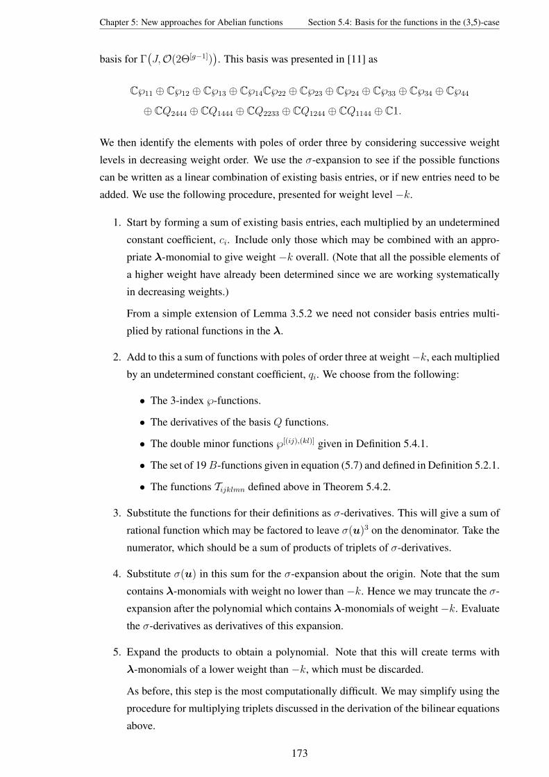
Chapter 5: New approaches for Abelian functions Section 5.4: Basis for the functions in the (3,5)-case
basis for Γ(J,O(2Θ[g−1])
). This basis was presented in [11] as
C℘11 ⊕ C℘12 ⊕ C℘13 ⊕ C℘14C℘22 ⊕ C℘23 ⊕ C℘24 ⊕ C℘33 ⊕ C℘34 ⊕ C℘44
⊕ CQ2444 ⊕ CQ1444 ⊕ CQ2233 ⊕ CQ1244 ⊕ CQ1144 ⊕ C1.
We then identify the elements with poles of order three by considering successive weight
levels in decreasing weight order. We use the σ-expansion to see if the possible functions
can be written as a linear combination of existing basis entries, or if new entries need to be
added. We use the following procedure, presented for weight level −k.
1. Start by forming a sum of existing basis entries, each multiplied by an undetermined
constant coefficient, ci. Include only those which may be combined with an appro-
priate λ-monomial to give weight −k overall. (Note that all the possible elements of
a higher weight have already been determined since we are working systematically
in decreasing weights.)
From a simple extension of Lemma 3.5.2 we need not consider basis entries multi-
plied by rational functions in the λ.
2. Add to this a sum of functions with poles of order three at weight−k, each multiplied
by an undetermined constant coefficient, qi. We choose from the following:
• The 3-index ℘-functions.
• The derivatives of the basis Q functions.
• The double minor functions ℘[(ij),(kl)] given in Definition 5.4.1.
• The set of 19B-functions given in equation (5.7) and defined in Definition 5.2.1.
• The functions Tijklmn defined above in Theorem 5.4.2.
3. Substitute the functions for their definitions as σ-derivatives. This will give a sum of
rational function which may be factored to leave σ(u)3 on the denominator. Take the
numerator, which should be a sum of products of triplets of σ-derivatives.
4. Substitute σ(u) in this sum for the σ-expansion about the origin. Note that the sum
contains λ-monomials with weight no lower than −k. Hence we may truncate the σ-
expansion after the polynomial which contains λ-monomials of weight−k. Evaluate
the σ-derivatives as derivatives of this expansion.
5. Expand the products to obtain a polynomial. Note that this will create terms with
λ-monomials of a lower weight than −k, which must be discarded.
As before, this step is the most computationally difficult. We may simplify using the
procedure for multiplying triplets discussed in the derivation of the bilinear equations
above.
173

Chapter 5: New approaches for Abelian functions Section 5.4: Basis for the functions in the (3,5)-case
To save further computation time and memory distributed computing may be em-
ployed to expand the products in parallel.
6. Collect this polynomial into a sum of the various uλ-monomials with coefficients
linear in the unknown constants ci, qi.
7. Consider these coefficients as a series of linear equations in the unknowns that must
equal zero and solve for the unknowns.
• If there is a unique solution for the ci in terms of the qi then each of the functions
at weight−k may be expressed as a linear combination of existing basis entries.
• If this is not possible then add the necessary functions to the basis.
We have implemented this procedure in Maple and the corresponding Maple worksheet
may be found in the extra Appendix of files. It has allowed us to identify 80 of the 34 = 81
entries in the following basis.
C1 ⊕ C℘11 ⊕ C℘12 ⊕ C℘13 ⊕ C℘14
⊕ C℘22 ⊕ C℘23 ⊕ C℘24 ⊕ C℘33 ⊕ C℘34
⊕ C℘44 ⊕ CQ2444 ⊕ CQ1444 ⊕ CQ2233 ⊕ CQ1244
⊕ CQ1144 ⊕ C℘111 ⊕ C℘112 ⊕ C℘113 ⊕ C℘114
⊕ C℘122 ⊕ C℘123 ⊕ C℘124 ⊕ C℘133 ⊕ C℘134
⊕ C℘144 ⊕ C℘222 ⊕ C℘223 ⊕ C℘224 ⊕ C℘233
⊕ C℘234 ⊕ C℘244 ⊕ C℘333 ⊕ C℘334 ⊕ C℘344
⊕ C℘444 ⊕ C∂4Q2444 ⊕ C∂3Q2444 ⊕ C∂4Q1444 ⊕ C∂2Q2444
⊕ C∂3Q1444 ⊕ C∂4Q2233 ⊕ C∂4Q1244 ⊕ C∂4Q1144 ⊕ C∂1Q1444
⊕ C∂2Q1244 ⊕ C∂3Q1244 ⊕ C∂2Q2233 ⊕ C∂3Q1144 ⊕ C∂1Q2233
⊕ C∂1Q1244 ⊕ C∂2Q1144 ⊕ C∂1Q1144 ⊕ C℘[(34),(34)] ⊕ C℘[(24),(34)]
⊕ C℘[(23),(34)] ⊕ C℘[(24),(24)] ⊕ C℘[(23),(24)] ⊕ C℘[(14),(34)] ⊕ C℘[(13),(34)]
⊕ C℘[(23),(23)] ⊕ C℘[(14),(24)] ⊕ C℘[(13),(24)] ⊕ C℘[(14),(23)] ⊕ C℘[(13),(23)]
⊕ C℘[(14),(14)] ⊕ C℘[(12),(24)] ⊕ C℘[(13),(14)] ⊕ C℘[(12),(23)] ⊕ C℘[(13),(13)]
⊕ C℘[(12),(14)] ⊕ C℘[(12),(13)] ⊕ C℘[(12),(12)] ⊕ CBA22244 ⊕ CBB
12444
⊕ CT133344 ⊕ CT114444 ⊕ CT222233 ⊕ CT222224 ⊕ CT222222
⊕ ?
Note that the derivatives of basis Q-functions have been included instead of many of the
B-functions used in Section 5.2.4. However, they occur at the same weight levels and so
play the same role. The basis currently includes 41 even functions and 39 odd functions, but
it is not known what parity the final function should have. An additional class of functions
will be required to identify the final basis element. It is possible that the identification of
such a function may aid the derivation of the missing quadratic 3-index relations at weight
−24. Clearly, this is an important problem for further research.
174

Chapter 6
Reductions of the Benney equations
6.1 Introduction
This Chapter develops an application of the theory of Abelian functions to a problem in
non-linear differential equations. An explicit example is presented which uses the results
of Chapter 3 for the multiply periodic functions associated with the cyclic (4,5)-curve.
The material in this chapter was recently summarised and published in [40] which was
co authored by Dr. John Gibbons. Some of the more lengthly results discussed here may
be found in the extra Appendix of files, or online at [37]. The Maple worksheets in which
the results were calculated are also available in the extra Appendix of files.
In [48] and [49] it was shown that Benney’s moment equations
Ant = An+1x + nAn−1A0
x, n ≥ 0,
admit reductions in which only finitely many N of the moments An are independent. Fur-
ther, it was shown that a large class of such reductions may be parametrised by conformal
maps from an upper half plane to a slit domain — an upper half plane cut along N non in-
tersecting curves with one fixed end point on the real line and the other free end a Riemann
invariant of the reduced equations.
A natural subclass of these occur where the curves of the slit domain are straight lines,
leading to a polygonal domain and an N -parameter Schwartz-Christoffel map. An impor-
tant and tractable subfamily of these is the case in which the angles are all rational multiples
of π. In [73] it was shown that this subclass leads to a mapping given by an integral of a
second kind Abelian differential on an algebraic curve. Such examples have been worked
out explicitly, in [73], [12], [13] and [14]. In all these examples the underlying curves have
been from the class of (n, s)-curves, with the reductions constructed explicitly by evaluat-
ing both the integrand and its integral using quotients of σ-derivatives associated with the
respective curves.
175

Chapter 6: Reductions of the Benney equations Section 6.1: Introduction
These papers have considered elliptic and hyperelliptic curves as well as a cyclic trig-
onal example. In this chapter we generalise the approach to the tetragonal curve that was
discussed in Chapter 3. We develop new methods which should now be easily applied to
reductions related to any (n, s)-curve.
This chapter is organised as follows. First background information of the Benney equa-
tions and the reductions is presented in Section 6.2. Then, in Section 6.3, the particular
reduction associated with the tetragonal curve is developed, with the necessary theory in-
troduced. In Section 6.4 we derive relations between the σ-derivatives that hold on the var-
ious strata of the Jacobian, with the relations themselves available in Appendix E. These
relations allows us to evaluate the mapping integrand in Section 6.5 and obtain an explicit
formula in Section 6.6.
176

Chapter 6: Reductions of the Benney equations Section 6.2: Benney’s equations
6.2 Benney’s equations
In 1973 Benney published [17] which considered an approximation for the two-dimensional
equations of motion of an incompressible perfect fluid under a gravitational force. He
showed that if moments are defined by
An(x, t) =
∫ h
0
vn dy, (6.1)
where v(x, y, t) is the horizontal fluid velocity and h(x, t) the height of the free surface, then
the momentsAn(x, t) satisfy an infinite set of hydrodynamic type equations, now called the
Benney moment equations.
Definition 6.2.1. The Benney moment equations are the following infinite set of partial
differential equations.
∂An∂t
+∂An+1
∂x+ nAn−1
∂A0
∂x= 0 n = 1, 2, . . . (6.2)
Identical moment equations were alternatively derived from a Vlasov equation in
[44], [74]. In this case the moments were defined by
An =
∫ ∞−∞
pnf dp (6.3)
where f = f(x, q, t) is a distribution function.
Benney showed in [17] that system (6.2) has infinitely many conserved densities, poly-
nomial in the An. One of the most direct ways to calculate these is to use generating
functions as described in [52]. Let q(x, p, t), be the series in p which acts as a generating
function of the moments,
q(x, p, t) = p+∞∑n=0
Anpn+1
, (6.4)
and let p(x, q, t) be the inverse series,
p(x, q, t) = q −∞∑m=0
Hm
qm+1.
We note here that if equation (6.3) is substituted into equation (6.4), then we obtain the
asymptotic series, as p→∞, of an integral,
q = p+
∫ ∞−∞
f(x, p′, t)
(p− p′)dp′. (6.5)
Here p′ runs along the real axis, and we take Im(p) > 0. It follows that q(p) is holomorphic
in its domain of definition.
177

Chapter 6: Reductions of the Benney equations Section 6.2: Benney’s equations
Comparing the first derivatives of q(x, p, t), we obtain the differential equation
∂q
∂t+ p
∂q
∂x=∂q
∂p
(∂p
∂t+ p
∂p
∂x+∂A0
∂x
). (6.6)
If we now hold p constant, we obtain the same form of Vlasov equation from which the
moments were defined. Hence any function of q and f must satisfy the same equation.
Alternatively, if we hold q constant in equation (6.6), then we obtain the conservation
equation,∂p
∂t+
∂
∂x
(1
2p2 + A0
)= 0. (6.7)
Substituting the formal series of p(x, q, t) into equation (6.7), we see that each Hn is poly-
nomial in the An and is a conserved density.
6.2.1 Reductions of the moment equations
Suppose that for some family of points, p = pi(x, t), q(pi) = qi(x, t), we have
∂q
∂p
∣∣∣∣p=pi
= 0.
Then equation (6.6) reduces to∂qi∂t
+ pi∂qi∂x
= 0,
where∂qi∂t
=∂q
∂t
∣∣∣∣p=pi
and∂qi∂x
=∂q
∂x
∣∣∣∣p=pi
.
We say that qi is a Riemann invariant with characteristic speed pi. We will see that there
are families of functions q(p) which are invariant under the Benney dynamics, and are
parametrised by N Riemann invariants qi.
A hydrodynamic type system with N ≥ 3 independent variables can not in general
be expressed in terms of Riemann invariants. If such a system does have N Riemann
invariants, it is called diagonalisable. Using results from Tsarev in [66] we can conclude
that any system of this type can be solved in principle using the method of a hodograph
transformation.
This construction cannot easily be applied to the Benney equations however, as these
have infinitely many dependent variables. Instead we must consider families of distribution
functions f , which are parameterised by finitely many, N , Riemann invariants qi(x, t).
Definition 6.2.2. Consider the case where the function q(p, x, t) is such that only N of the
moments are independent. In [48] and [49] we find this implies N characteristic speeds,
assumed real and distinct, and N corresponding Riemann invariants (pi, qi). In this case
Benney’s equations reduce to a diagonal system of hydrodynamic type with finitely many
178

Chapter 6: Reductions of the Benney equations Section 6.2: Benney’s equations
dependent variables qi.
∂qi∂t
+ pi(q)∂qi∂x
= 0, i = 1, 2, . . . , N. (6.8)
Such a system is called a reduction of Benney’s equations.
The construction of a general family of solutions for equations of this type was outlined
in [48] and [49].
6.2.2 Schwartz-Christoffel reductions
Recall that q must map from the upper half p-plane to an upper half plane. Explicit solutions
have been constructed in the case where the mapping function maps to a polygonal N -slit
domain.
Definition 6.2.3. We define polygonal N -slit domain as follows. Suppose the real p-axis
has M vertices marked on it and the preimage in the p-plane of each slit runs from a vertex
pj to a point vi, the preimage of the end of the slit, and then to another vertex pj+1. The
angle π in the p-plane at pj is mapped to an angle αjπ at the image point. The internal
angle at the end of each slit is 2π.
In this case the mapping function is shown to be given, up to a constant of integration,
by
q =
∫ p[ ∏N
i=1(p− vi)∏2Nj=1(p− pj)1−αj
]dp.
If the integrand is to converge to one as p→∞, we require
2N∑j=1
αj = N.
To avoid a logarithmic singularity, we further impose,
M∑j=1
αj pj =N∑i=1
vi.
We may then define q more precisely as follows.
Definition 6.2.4. Define q to be a Schwartz-Christoffel mapping if it is of the form
q = p+
∫ p
−∞
[ ∏Ni=1(p− vi)∏M
j=1(p− pj)1−αj− 1
]dp.
Other constraints are imposed by requiring the vertices pj to map to points q0i , the fixed
base points of the slits. There remain N independent parameters, which can be taken to be
179

Chapter 6: Reductions of the Benney equations Section 6.2: Benney’s equations
the movable end points of the slits qi(x, t). These satisfy the equations of motion
∂qi∂t
+ vi∂qi∂x
= 0.
Hence, to use the general solution to these equations we must evaluate the Schwartz-
Christoffel integral explicitly.
Example 6.2.5. An elementary example is the case where the map takes the upper half
p-plane to the upper half q-plane with a vertical slit, as shown in Figure 6.1.
Figure 6.1: The domain and codomain of the map in Example 6.2.5
This relates to the following Schwarz-Christoffel map.
q(p) = p+
∫ p
∞
p′ − v1√(p′ − p1)(p′ − p2)
dp′.
If the residue at infinity is set to be zero, then this imposes the condition v1 = 12(p1 + p2)
and we get the solution
q(p) = v1 +√p2 − (p1 + p2)p+ p1p2
= v1 +√
(p− v1)2 + 2A0,
(from the expansion as p→∞). The two parameters p1 and p2 are not independent, as for
consistency their sum must be a constant. Hence only the end point of the slit in the q-plane
is variable. This is the Riemann invariant.
The most tractable cases are where all the αj are rational, so that the integrand becomes
a meromorphic second kind differential on some algebraic curve. In this case the only
singularity is as p → ∞, where the integrand has a double pole with no residue, and the
integral thus has a simple pole.
The integral has been calculated explicitly in [73], [12], [13] and [14], in each case using
the theory of (n, s)-curves. These papers have considered elliptic and hyperelliptic curves
as well as a cyclic trigonal example. In each case the mappings were found as rational
functions of derivatives of the Kleinian σ-function of the associated curve.
180

Chapter 6: Reductions of the Benney equations Section 6.3: A tetragonal reduction
6.3 A tetragonal reduction
We will consider reductions that allow us to work on a tetragonal surface, which has not
been considered before in the context of this application. The first step is to specify the do-
main and codomain of the mapping q for this case. For the reduction to involve a tetragonal
surface we will require two or more sets of straight slits, making angles of π/4, π/2, and
3π/4 to the horizontal.
Define P to be the upper half p-plane with 14 points marked on the real axis, as in
Figure 6.2.
Figure 6.2: The domain P within the p-plane.
These points satisfy
p1 < v1 < p2 < v2 < p3 < v3 < p4 < p5 < v4 < p6 < v5 < p7 < v6 < p8.
Then define the codomainQ′ as the upper-half q-plane with two triplets of slits, as described
above. We let the first trio of slits radiate from the fixed point p1, with the end points of
these three slits labeled v1, v2 and v3 respectively. Similarly, let the second trio of slits
radiate from p5 and have end points v4, v5, v6. Finally impose the conditions that
q(pi) = pi, p1 = p2 = p3 = p4,
q(vi) = vi, p5 = p6 = p7 = p8.
We then see thatQ′ is the slit domain as shown in Figure 6.3, and the mapping q : P → Q′
can be given in Schwartz Christoffel form by
q(p) = p+
∫ p
∞
[ϕ(p′)− 1
]dp′ (6.9)
with
ϕ(p) =
∏6i=1(p− vi)[∏8i−1(p− pi)
] 34
=
∏6i=1(p− vi)Y 3
, (6.10)
where
Y 4 =8∏i=1
(p− pi). (6.11)
181

Chapter 6: Reductions of the Benney equations Section 6.3: A tetragonal reduction
Figure 6.3: The domain Q′ within the q-plane.
Note that we require the following zero residue property.
limp→∞
ϕ(p) ∼ 1 +O
(1
p2
). (6.12)
This mapping would lead us to consider the Riemann surface given by points (p, Y )
that satisfy equation (6.11). However, we wish to consider the simplest possible tetragonal
surface (one with only six branch points) and so we collapse two of the slits, (the final two
by choice). This simplifies our q-plane to Q, given in Figure 6.4. Our problem will be to
determine an explicit formula for the mapping q(p) in this case.
Figure 6.4: The domain Q within the q-plane.
As in the trigonal case, the analysis of this surface is eased if we put it into canonical
form, by mapping one of the branch points, (p8 by choice), to infinity.
We use the following invertible rational map to perform these simplifications on our
curve and integrand.
p6 = p8, p7 = p8, v5 = p8, v6 = p8,
p = p8 −(
1
x
), pi = p8 −
1
Ti, i = 1, . . . , 5, (6.13)
Y =yk
x2where k4 = −
5∏i=1
(p8 − pi) = −5∏i=1
1
Ti.
182

Chapter 6: Reductions of the Benney equations Section 6.3: A tetragonal reduction
If we perform the mapping (6.13) on the curve (6.11) we obtain
y4k4
x8=
[5∏i=1
(p8 −
1
x− p8 +
1
Ti
)](p8 −
1
x− p8
)3
= − 1
x3
5∏i=1
(1
Ti− 1
x
)
= − 1
x3
[5∏i=1
(x− Ti)1
xTi
]=
[5∏i=1
(x− Ti)
]·(
1
x8
)· (−1)
[5∏i=1
1
Ti
].
This simplifies to give the following canonical form of the curve (6.11).
y4 =5∏i=1
(x− Ti)
= x5 + λ4x4 + λ3x
3 + λ2x2 + λ1x+ λ0, (6.14)
for constants λ0, . . . , λ4. Let C denote the Riemann surface defined by equation (6.14).
We now consider q(p) as mappingP → Q by performing (6.13) on the integrand (6.10).
ϕ(p)dp =
(x6
y3k3
)[ 4∏i=1
(p8 −
1
x− vi
)](p8 −
1
x− p8
)2(− 1
x2dx
)
=
(x6
y3k3
)[ 4∏i=1
((p8 − vi)x− 1)
] [1
x4
](1
x
)2(− 1
x2dx
)= K
[A4x
4 + A3x3 + A2x
2 + A1x+ 1] 1
x2
dx
4y3≡ ϕ(x)dx, (6.15)
where K = −4/k3 and A1, . . . , A4 are constants. We consider this transformed integrand
as varying with x instead of p and so denote it ϕ(x)dx. We will evaluate this integrand
using Kleinian functions defined upon C.
The tetragonal surface C
Equation (6.14) is the cyclic tetragonal curve of genus six that was studied in detail in
Chapter 3. The surface is constructed from four sheets of the complex plane, with branch
points of order four at
T1, T2, T3, T4, T5, T6 =∞,
and branch cuts along the intervals
[T1, T2], [T2, T3], [T3, T4], [T5,∞].
In Section 3.1 we constructed the standard basis of holomorphic differentials upon C, de-
noted du and given in equation (3.4).
183

Chapter 6: Reductions of the Benney equations Section 6.3: A tetragonal reduction
Any point u ∈ C6 can be expressed as
u = (u1, u2, u3, u4, u5, u6) =6∑i=1
∫ Pi
∞du,
where the Pi are six variable points upon C.
In Chapter 3 we used the Kleinian σ-function defined in association with C to construct
and investigate the Abelian functions associated with C. In this chapter we will use the
σ-function to evaluate the integral q(x).
Recall the Abel map, defined in Definition 2.2.13, that mapped points on the curve to
the Jacobian. We denoted the image of the kth Abel map by W [k] and in Definition 2.2.14
defined strata of the Jacobian as
Θ[k] = W [k] ∪ [−1]W [k].
In fact, since this (n, s)-curve has n = 4 which is even the process is simplified and we
have
W [k] = [−1]W [k] = Θ[k].
When k = 1 the Abel map gives a one dimensional image of the curve C. Since our
mapping was given by a single integral with respect to one parameter, it will make sense to
rewrite this as an integral on the one-dimensional strata, Θ[1]. In addition to [12], [13] and
[14], similar problems of inverting meromorphic differentials on lower dimensional strata
of the Jacobian have been studied, in the case of hyperelliptic surfaces, in [41], [47], [1]
and [2] for example.
184

Chapter 6: Reductions of the Benney equations Section 6.4: Relations between the σ-derivatives
6.4 Relations between the σ-derivatives
In Section 6.5 we will evaluate the integrand (6.15) as a function of σ-derivatives restricted
to Θ[1]. In order to achieve this we will first need to derive equations that hold between the
various σ-derivatives when u ∈ Θ[1]. In Chapter 3 sets of relations between the Abelian
functions associated with C were calculated. However, these were the relations that held
everywhere, and do not give us sufficient information for the behaviour of σ(u) on the
various strata.
We start in Section 6.4.1 by deriving those relations that define the various strata. Then
in Section 6.4.2 we obtain further relations from these through a technique we have devel-
oped known as descending. (Essentially since each relation on Θk is also valid on Θk−1 we
can consider the effect on it as u descends the strata.)
6.4.1 The defining strata relations
Recall from Lemma 2.2.19 that Θ[g−1] may be defined as those places where σ(u) = 0.
Θ[5] = u | σ(u) = 0.
We may derive similar defining relations for the other strata using the following theorem of
Jorgenson, (from [50]).
Theorem 6.4.1. Let u ∈ Θ[k] for some k < g. Then for a set of k points Pi = (xi, yi) on C
we have
u =k∑i=1
∫ Pi
∞du,
and the following statement holds for vectors a, b of arbitrary constants.∑gj=1 ajσj(u)∑gj=1 bjσj(u)
=det[a∣∣du(P1)
∣∣ · · · ∣∣du(Pk)∣∣du(Pk)
(g−k−1)∣∣ · · · ∣∣du(Pk)
(1)]
det[b∣∣du(P1)
∣∣ · · · ∣∣du(Pk)∣∣du(Pk)(g−k−1)
∣∣ · · · ∣∣du(Pk)(1)] .
Here, du(i) denotes the column of ith derivatives of the holomorphic differentials du, and
should be ignored if i < 1.
Start by considering Theorem 6.4.1 in the case when k = 5. Then for arbitrary a, b∑6j=1 ajσj(u)∑6j=1 bjσj(u)
=det[a∣∣du(P1)
∣∣ · · · ∣∣du(P5)]
det[b∣∣du(P1)
∣∣ · · · ∣∣du(P5)] .
Now, as u ∈ Θ[5] approaches Θ[4] we must have one of the points Pi approaching∞. Let
P5 = (x5, y5) approach∞ and use the local coordinate ξ to replace the final column of the
determinants by the expansions for du in ξ. (These expansions were derived in Chapter 3
in equation (3.24) and are summarised below. However, for these calculations we will need
185

Chapter 6: Reductions of the Benney equations Section 6.4: Relations between the σ-derivatives
more terms and so refer to the longer expansions presented in Appendix C.1).
du1 = [−ξ10 +O(ξ14)]dξ, du4 = [−ξ2 + 34λ4ξ
6 +O(ξ10)]dξ,
du2 = [−ξ6 +O(ξ10)]dξ, du5 = [−ξ1 + 12λ4ξ
5 +O(ξ9)]dξ,
du3 = [−ξ5 +O(ξ9)]dξ, du6 = [−1 + 14λ4ξ
4 +O(ξ8)]dξ.
(6.16)
When u arrives at Θ[4] we have ξ = 0 and hence the determinant in the numerator becomes
∣∣∣∣∣∣∣∣∣∣∣∣∣∣∣∣∣∣∣∣∣∣∣
a1dx1
4y31
· · · dx4
4y34
0
a2x1dx1
4y31
· · · x4dx4
4y34
0
a3y1dx1
4y31
· · · y4dx4
4y34
0
a4x2
1dx1
4y31
· · · x24dx4
4y34
0
a5x1y1dx1
4y31
· · · x4y4dx4
4y34
0
a6y2
1dx1
4y31
· · · y24dx4
4y34
−1
∣∣∣∣∣∣∣∣∣∣∣∣∣∣∣∣∣∣∣∣∣∣∣
+
=
(dx1
4y31
· · · dx4
4y34
)+
×
∣∣∣∣∣∣∣∣∣∣∣∣∣∣∣∣
a1 1 · · · 1 0
a2 x1 · · · x4 0
a3 y1 · · · y4 0
a4 x21 · · · x2
4 0
a5 x1y1 · · · x4y4 0
a6 y21 · · · y2
4 −1
∣∣∣∣∣∣∣∣∣∣∣∣∣∣∣∣.
The determinant in the denominator will be identical, except with the entries of a replaced
by the entries of b. Hence the factored terms will cancel, leaving us with the simpler
determinants. It is clear from the final column, that when we expand the determinants the
resulting quotient of polynomials will not vary with the arbitrary constant a6.∑gj=1 ajσj(u)∑gj=1 bjσj(u)
= function that does not vary with a6.
Since a6 can be any constant we must conclude that for u ∈ Θ[4], the function σ6(u) = 0.
(Note the same conclusion could have been drawn from considering the constant b6.)
Θ[4] = u | σ(u) = σ6(u) = 0.
We repeat this process by considering Theorem 6.4.1 in the case when k = 4.∑6j=1 ajσj(u)∑6j=1 bjσj(u)
=det[a∣∣du(P1)
∣∣ · · · ∣∣du(P4)∣∣du(P4)(1)
]det[b∣∣du(P1)
∣∣ · · · ∣∣du(P4)∣∣du(P4)(1)
] .This time we consider u descending to Θ[3], by letting the fourth point move towards infin-
ity. The penultimate column in each determinant can be given with the expansions (6.16) as
before. For the final column we will need to determine the derivative of these expansions.
d2u1
dξ2= −10ξ9 +O(ξ13),
d2u4
dξ= −2ξ + 9
2λ4ξ
5 +O(ξ9),
186

Chapter 6: Reductions of the Benney equations Section 6.4: Relations between the σ-derivatives
d2u2
dξ2= −6ξ5 +O(ξ9),
d2u5
dξ2= −1 + 5
2λ4ξ
4 +O(ξ8),
d2u3
dξ2= −5ξ4 +O(ξ8),
d2u6
dξ2= λ4ξ
3 +O(ξ7). (6.17)
When u arrives at Θ[3] we will have ξ = 0. Our determinants will again factor and cancel
to leave the numerator as ∣∣∣∣∣∣∣∣∣∣∣∣∣∣∣∣
a1 1 · · · 1 0 0
a2 x1 · · · x3 0 0
a3 y1 · · · y3 0 0
a4 x21 · · · x2
3 0 0
a5 x1y1 · · · x3y3 0 −1
a6 y21 · · · y2
3 −1 0
∣∣∣∣∣∣∣∣∣∣∣∣∣∣∣∣with the denominator identical except for b instead of a. From the final two columns it is
clear that the resulting quotient of polynomials will not vary with the arbitrary constants a6
and a5. Hence we must conclude that
Θ[3] = u | σ(u) = σ6(u) = σ5(u) = 0.
We repeat the procedure once more for k = 3.∑6j=1 ajσj(u)∑6j=1 bjσj(u)
=det[a∣∣du(P1)
∣∣ · · · ∣∣du(P3)∣∣du(P3)(1)
∣∣du(P3)(2)]
det[b∣∣du(P1)
∣∣ · · · ∣∣du(P3)∣∣du(P3)(1)
∣∣du(P3)(2)] .
We let u descend to Θ[2] and use the expansions (6.16) and (6.17) for the fourth and fifth
columns. The final column will require the derivatives of the expansions in (6.17).
d3u1
dξ3= −90ξ8 +O(ξ12),
d3u34
dξ= −2 + 45
2λ4ξ
4 +O(ξ8),
d3u2
dξ3= −30ξ4 +O(ξ8),
d3u5
dξ3= 10λ4ξ
3 +O(ξ7), (6.18)
d3u3
dξ3= −20ξ3 +O(ξ7),
d3u6
dξ3= 3λ4ξ
2 +O(ξ6).
We let ξ = 0 and cancel the common factors to leave the numerator as∣∣∣∣∣∣∣∣∣∣∣∣∣∣∣∣
a1 1 · · · 1 0 0 0
a2 x1 · · · x2 0 0 0
a3 y1 · · · y2 0 0 −2
a4 x21 · · · x2
2 0 0 0
a5 x1y1 · · · x2y2 0 −1 0
a6 y21 · · · y2
2 −1 0 0
∣∣∣∣∣∣∣∣∣∣∣∣∣∣∣∣187

Chapter 6: Reductions of the Benney equations Section 6.4: Relations between the σ-derivatives
and similarly for the denominator. Expand the determinants and the statement reduces to∑6j=1 ajσj(u)∑6j=1 bjσj(u)
=a1x1y2 − a1y1x2 + a2y1 − a2y2 − a3x1 + a3x2
b1x1y2 − b1y1x2 + b2y1 − b2y2 − b3x1 + b3x2
(6.19)
for u ∈ Θ[2]. The right hand side is the same for all values of a6, a5, a4 and hence we
conclude that
Θ[2] = u | σ(u) = σ6(u) = σ5(u) = σ4(u) = 0.
Finally we consider Theorem 6.4.1 in the case when k = 2. Here, when we let u descend
to Θ[1], we find that the statement of the Theorem involves singular matrices. (Consider
a further derivative of the series in (6.18). All these series would vanish when ξ is set to
zero.) Hence this time the theorem will give us no information.
Instead we can consider equation (6.19) which held for u ∈ Θ[2]. Let u descend to Θ[1]
here, by replacing (x2, y2) by their expansions in ξ, given in equations (3.22) and (3.23).
We find that ∑6j=1 ajσj(u)∑6j=1 bjσj(u)
=a1x1 − a2
b1x1 − b2
+O(ξ). (6.20)
When u ∈ Θ[1] we set ξ = 0 and conclude that the right hand side has no dependence on
a3, a4, a5 or a6. Hence
Θ[1] = u | σ(u) = σ6(u) = σ5(u) = σ4(u) = σ3(u) = 0.
Note that there is a Maple worksheet available in the extra Appendix of files in which these
calculations are performed.
Summary
The strata of C can be defined by the zeros of the σ-function and its derivatives as follows.
The definition of Θ[5] is a classical result (Lemma 2.2.19), while the others were derived
from Theorem 6.4.1.
Θ[5] = u | σ(u) = 0
Θ[4] = u | σ(u) = σ6(u) = 0
Θ[3] = u | σ(u) = σ6(u) = σ5(u) = 0 (6.21)
Θ[2] = u | σ(u) = σ6(u) = σ5(u) = σ4(u) = 0
Θ[1] = u | σ(u) = σ6(u) = σ5(u) = σ4(u) = σ3(u) = 0
188

Chapter 6: Reductions of the Benney equations Section 6.4: Relations between the σ-derivatives
6.4.2 Further relations
We next use the defining strata relations (6.21) to generate further relations between the
σ-derivatives, holding on each strata. We use a systematic method, implemented in Maple,
to achieve this.
Start with the relation σ(u) = 0, valid for u ∈ Θ[5]. Consider u ∈ Θ[5] as it descends
to Θ[4]. We write u as u = u+ uξ where u is an arbitrary point on Θ[4] and uξ is a vector
containing the series expansions of u. (These may be obtained by integrating (6.16) or refer
to the larger expansions are presented in Appendix C.1.) We calculate the series expansion
of σ(u+ uξ) = 0 in ξ as
0 = σ(u+ uξ) = σ(u)− σ6(u)ξ + 12
[σ66(u)− σ5(u)
]ξ2 +
[12σ56(u)− 1
6σ666(u)
− 13σ4(u)
]ξ3 +
[18σ55(u) + 1
3σ46(u)− 1
4σ566(u) + 1
24σ6666(u)
]ξ4 +
[− 1
120σ66666(u)
+ 112σ5666(u) + 1
6σ45(u)− 1
6σ466(u)− 1
8σ556(u) + 1
20σ6(u)λ4
]ξ5 +O
(ξ6). (6.22)
Setting the coefficients of ξ to zero gives us a set of relations for u ∈ Θ[4].
σ6(u) = 0
σ66(u) = σ5(u)
σ666(u) = 3σ56(u)− 2σ4(u) (6.23)
σ6666(u) = 6σ566(u)− 8σ46(u)− 3σ55(u)
σ66666(u) = 10σ5666(u)− 20σ466(u)− 15σ556(u) + 20σ45(u) + 6λ4σ6(u)
...
If we calculate the expansion to a higher order of ξ then infinitely more relations can be
obtained, involving progressively higher index σ-derivatives. Note however, that the ex-
pansions for uξ must first be calculated to a sufficiently high order first. Using the Maple
series command we find that the series in equation (6.22) continues with
. . .+[
1720σ666666 − 1
48σ56666 − 1
48σ555 + 1
16σ5566 − 1
6σ3 + 1
18σ44 + 1
12σ5λ4
+ 118σ4666 − 1
6σ456 − 1
20σ66λ4
]ξ6 +
[148σ5556 + 1
240σ566666 − 1
24σ455 − 1
18σ446
+ 328σ4λ4 + 1
12σ4566 − 1
7σ2 − 1
72σ46666 − 1
5040σ6666666 − 1
48σ55666 + 1
6σ36
+ 140σ666λ4 − 13
120σ56λ4
]ξ7 +
[1
360σ466666 + 1
192σ556666 − 1
96σ55566 + 1
36σ4466
+ 112σ35 + 1
7σ26 + 1
40320σ66666666 − 13
105σ46λ4 − 1
36σ445 + 1
384σ5555 + 1
24σ4556
− 11440
σ5666666 − 112σ366 − 1
120σ6666λ4 − 1
24σ55λ4 − 1
36σ45666 + 1
15σ566λ4
]ξ8
. . .+[
1144σ4555 − 1
12σ356 + 1
36σ4456 − 1
162σ444 − 1
14σ266 − 1
384σ55556 + 59
840σ466λ4
− 19720σ5666λ4 + 1
36σ6λ3 − 5
288σ6λ4
2 + 1480σ66666λ4 − 1
362880σ666666666 + 1
18σ34 + . . .
189

Chapter 6: Reductions of the Benney equations Section 6.4: Relations between the σ-derivatives
· · ·+ 114σ25 + 1
144σ456666 + 1
288σ555666 − 1
48σ45566 − 1
2160σ4666666 − 1
960σ5566666
+ 110080
σ56666666 + 23480λ4σ556 − 1
108σ44666 − 41
504λ4σ45 + 1
36σ3666
]ξ9 +O
(ξ10).
We have calculated an expansion for σ(u+uξ) up toO(ξ29), generating a set of 28 relations
for the σ-derivatives valid for u ∈ Θ[4]. Note that the standard Maple series command
was not able to derive an expansion further than O(ξ14) due to memory constraints. Instead
an alternative procedure was implemented, making use of the weight properties described
in Section 3.3.
Recall that the σ-function has a definite Sato weight, which is +15 in the case of the
cyclic (4,5)-curve. Hence this expansion in ξ must also be homogeneous with this weight,
(check series (6.22) to see this is the case). Since ξ has weight one we know the coefficient
of ξn must be a sum of terms with weight 15 − n. Hence we can determine which σ-
derivatives may be present, (those that can be combined with a λ-monomial to give the
correct weight).
We write a procedure that calculates each coefficient of ξ successively. Recall that the
expansions ofu in ξ also involve terms with decreasing λweight. At each stage we truncate
these expansions at the appropriate weight necessary to calculate the next coefficient. We
then calculate that coefficient only, (using the general equation for an unknown function of
six variables).
The remainder of the expansion and the full set of relations can be found in the extra
Appendix of files or online at [37]. The Maple worksheet in which the series is derived
using the new procedure can also be found in the extra Appendix of files.
The next step in this process will be to find the relations valid for u ∈ Θ[3]. Since
Θ[3] ⊂ Θ[4] we can conclude that the relations (6.23) for u ∈ Θ[4] are valid here also.
However, we can derive a larger set of relations for u ∈ Θ[3] by repeating the descent
procedure for all those relations valid for u ∈ Θ[4].
We do not need to consider the relation σ(u) = 0 since that will only give us the same
relations as above. Instead choose the second defining relation σ6(u) = 0. We again write
u = u+uξ where uξ is the vector of expansions as before and u is now an arbitrary point
on Θ[3]. Note that calculating the series expansion in ξ for σ6(u+ uξ) is not as arduous as
above. We can easily derive it from the expansion (6.22) for σ(u + uξ) by adding a six to
each index.
0 =(σ6 − σ66ξ + 1
2
[σ666 − σ56
]ξ2 +
[12σ566 − 1
3σ46 − 1
6σ6666
]ξ3 + · · ·
)(u)
Setting these coefficients of ξ to zero gives us more relations valid for u ∈ Θ[3], starting
with σ66(u) = 0. We can obtain further relations for u ∈ Θ[3] by descending all of the 28
relations in (6.23) for u ∈ Θ[4]. After this we find we have obtained 238 relations.
We need to organise these relations by choosing a ranking system to decide which σ-
190

Chapter 6: Reductions of the Benney equations Section 6.4: Relations between the σ-derivatives
derivatives should be expressed in terms of the others. It is logical to remove the higher
index σ-derivatives and so we always solve for those with the greater number of indices
first. (Note this was the approach that was taken with equations (6.23)). When we have the
choice between σ-derivatives with the same number of indices we choose to solve for those
with the highest numerical indices first.
So we take the 238 equations valid for u ∈ Θ[3], substitute in the equations for u ∈ Θ[4]
and solve according to these rules to give a set of equations in the σ-derivatives foru ∈ Θ[3].
The next step is to descend the relations valid for u ∈ Θ[3] to Θ[2]. We automate the
process of descending from Θ[k] to Θ[k−1] in Maple as follows.
1. Take a relation valid for u ∈ Θ[k] and expand as a series in ξ. To do this we replace each
σ-derivative by the series expansion for σ(u + uξ), adding the relevant index to each
σ-derivative in the expansion.
2. Set each coefficient with respect to ξ to zero, and save the resulting equations, valid for
u ∈ Θ[k−1].
3. Repeat Steps 1 and 2 for all known relations valid for u ∈ Θ[k] to obtain a large set of
equations between σ-derivatives, valid for u ∈ Θ[k−1].
4. Substitute the existing equations for u ∈ Θ[k] into the set. Then rearrange to obtain
additional equations for u ∈ Θ[k−1] by first solving for the higher index functions, and
then for those with the greater numerical indices.
So we use this process to obtain first a set of relations for u ∈ Θ[2] and then a final set
for u ∈ Θ[1]. (The corresponding Maple worksheet can be found in the extra Appendix
of files.) Appendix E.1 contains all the equations valid for u ∈ Θ[1] that express k-index
σ-derivatives with k ≤ 4. The full set of relations that have been derived for Θ[1], along
with the sets of relations for higher strata, can be found in the extra Appendix of files or
online at [37]. The most interesting result of these calculations was to find that on Θ[1] we
have
σ1(u) = σ2(u) = 0.
Together with equation (6.21) this shows that all the first derivatives of σ(u) are zero on
Θ[1]. (This may be double checked using the σ-expansion as derived in Section 3.4, and
then substituting in the expansions in ξ.)
This result is very surprising as it was not the case for the lower genus examples that
were considered. It also causes extra complications in the next Section.
Note that the calculations in this Section were computationally much more difficult that
those in [14]. The latter stages were performed in parallel on a small cluster of machines,
using Distributed Maple, (see [72]).
191

Chapter 6: Reductions of the Benney equations Section 6.5: Evaluating the integrand
6.5 Evaluating the integrand
Recall our integrand as given by equation (6.15),
ϕ(x)dx = K
(A4x
2 + A3x+ A2 +A1
x+
1
x2
)(dx
4y3
).
Now, the map q(x) was given by a single integral with respect to one parameter, the point
(x, y) on C. So we will rewrite this as an integral on the one-dimensional strata Θ[1] of J .
We will then evaluate it using σ-derivatives restricted to Θ[1]. In [14] Jorgenson’s Theorem
was used to express x in terms of σ-derivatives. However, if we followed this approach and
solved equation (6.20) for u ∈ Θ[1] we would find
x = −σ1(u)
σ2(u),
which makes no sense given that σ1(u) = 0 for u ∈ Θ[1]. Instead let us take equation
(6.19) which was also derived from Jorgenson’s Theorem and which holds for u in Θ[2].
We consider what happens to this as u descends to Θ[1]. We replace (x2, y2) with the
expansions in the parameter ξ and replace the σ-derivatives by their Taylor series in ξ. (The
expansions for x and y were given in equations (3.22) and (3.23) while the series of the
σ-derivatives is derived from equation (6.22) as discussed in the last section.) If we then
take a series expansion of this in ξ and set ξ = 0 we find that for u ∈ Θ[1] we have
a1σ23(u) + a2σ34(u)
b1σ23(u) + b2σ34(u)=a1x− a2
b1x− b2
.
Solving this for x gives,
x = −σ23(u)
σ34(u), (6.24)
for u ∈ Θ[1]. We must verify that σ34(u) is not identically zero on Θ[1]. Consider the expan-
sion about the origin that we derived in Chapter 3. Using the Schur-Weierstrass polynomial
(3.50) and the substitutions for u in ξ we see that
σ34(u) = ξ6 +O(ξ7),
and so σ34(u) is not identically zero. Further, this technique will allow us to specify all the
zeros of the function. First note that σ34(u) has exactly six zeros on Θ[1]. (The Riemann
vanishing theorem stated that the θ-function, and hence the σ-function, is either identically
zero or has exactly g = 6 zeros on the curve. The σ-derivatives may be defined using the
same θ-function, and while σ(u) is identically zero on Θ[1], not all the σ-derivatives are.)
Since the expansion above has a zero of order six at the origin, we can hence conclude that
σ34(u) restricted to Θ[1] cannot vanish for u 6= 0 mod Λ.
192

Chapter 6: Reductions of the Benney equations Section 6.5: Evaluating the integrand
Similarly, σ23(u) also has six zeros on Θ[1]. However,
σ23(u) = ξ2 +O(ξ3),
and hence there is a double zero at the origin and four other zeros corresponding to the
points x = 0 on each of the four sheets of C.
So we may evaluate x as the ratio of σ-derivatives in equation (6.24). Using this and
the standard basis of holomorphic differentials (3.4), we can rewrite our integrand as
ϕ(x)dx = K[ϕ1(x)dx+ ϕ2(x)dx] (6.25)
where
ϕ1(x)dx = A2du1 + A3du2 + A4du4, (6.26)
ϕ2(x)dx =
((σ34(u)
σ23(u)
)2
− A1σ34(u)
σ23(u)
)du1 ≡ ϕ2(u)du1. (6.27)
Thus ϕ1 is a sum of holomorphic differentials on C, and ϕ2 is a second kind meromorphic
differential. As in the lower genus examples, we will need to find a suitable function Ψ(u)
such thatd
du1
Ψ(u) = ϕ2(u), u ∈ Θ[1]. (6.28)
We will identify Ψ(u) and evaluate ϕ2(u) as follows. First we must derive the expan-
sions for ϕ2(u) at its poles. We will then find a function Ψ(u), which has simple poles
at the same points as the double poles of ϕ2(u), and which varies by at worst an additive
constant over the period lattice Λ.
The function Ψ(u) will be chosen so that ddu1
Ψ(u) has the same expansion at the poles
as ϕ2 and is regular elsewhere. It then follows that the difference ddu1
Ψ(u)− ϕ2(u) is both
holomorphic and Abelian. By the generalisation of Liouville’s theorem we can conclude
that this difference is a constant, which will be evaluated at a convenient point.
6.5.1 The expansion of ϕ2(u) at the poles
Recall that σ(u) was an entire function, and so ϕ2(u) will have poles at those points where
σ23(u) = 0. As discussed above, we know σ23(u) has six zeros — a double zero at the
origin and zeros at the four points, one on each sheet, where x = 0. We will first investigate
what happens at these four points and consider the origin later.
Recall the invariance condition on the cyclic (n, s)-curve given in equation (2.35). In
the (4,5)-case the cyclic symmetry is [i], the imaginary unit. This relates the four different
sheets and acts on (x, y) by
[i](x, y) 7→ (x, iy).
193

Chapter 6: Reductions of the Benney equations Section 6.5: Evaluating the integrand
Hence it will act on u as follows.
u1 7→ iu1 u2 7→ iu2 u3 7→ −u3
u4 7→ iu4 u5 7→ −u5 u6 7→ −iu6.(6.29)
Let u0 be the Abel image of the point on the principal sheet where σ23(u) = 0. This is the
point where x = 0 and y = (λ0)1/4. Then the four zeros of σ23(u) away from the origin are
given by
u0,N = [i]Nu0, N = 0, 1, 2, 3.
We will require the poles to match at all four of these points.
We need to find an expansion for ϕ2(u) at the points u0,N . To start, we consider
u ∈ Θ[1] and calculate the Taylor series of σ(u) around the point
u = u0 = (u0,1, u0,2, u0,3, u0,4, u0,5, u0,6).
Writing wi = (ui − u0,i) we have,
σ(u) = σ(u0) +[σ1(u0)w1 + σ2(u0)w2 + σ3w3(u0) + σ4(u0)w4
+ σ5(u0)w5 + σ6(u0)w6
]+[
12σ11(u0)w2
1 + σ12(u0)w1w2 + σ13(u0)w1w3
+ σ14(u0)w1w4 + σ15(u0)w1w5 + σ16(u0)w1w6 + 12σ22(u0)w2
2 + . . .
We will have similar expansions around the other u0,N . Note we can use this expansion to
easily compute the expansions for the σ-derivatives, (by simply adding the relevant indices).
Now, since u0,N are the points where t = 0, we can write their components as
(u0,N
)i
=
∫ 0
∞dui, i = 1, . . . , 6,
evaluated on the sheet where s = [i]N(λ0)1/4. Therefore we can denote
wi,N =(ui −
(u0,N
)i
)=
∫ x
∞dui −
∫ 0
∞dui =
∫ x
0
dui,
evaluated on the N th sheet. Using our basis of holomorphic differentials (3.4), we can find
expansions for w1,N , . . . w6,N in the parameter x.
w1,N =1
4
iN
λ03/4x− 3
32
i3Nλ1
λ07/4
x2 − i3N
128
8λ2λ0 − 7λ21
λ011/4
x3
− iN
2048
(96λ3λ02 − 168λ1λ2λ0 + 77λ1
3)
λ015/4
x4 +O(x5)
(6.30)
w2,N =1
8
iN
λ03/4x2 − 1
16
iNλ1
λ07/4x3 − 3iN
512
8λ2λ0 − 7λ12
λ011/4
x4 +O(x5)
194

Chapter 6: Reductions of the Benney equations Section 6.5: Evaluating the integrand
w3,N =1
4
i2N
λ1/20
x− 1
16
i2Nλ1
λ03/2
x2 − i2N
96
4λ2λ0 − 3λ12
λ05/2
x3
− i2N
256
8λ3λ02 − 12λ1λ2λ0 + 5λ1
3
λ07/2
x4 +O(x5)
w4,N =1
12
iN
λ03/4x3 − 3
64
iNλ1
λ07/4x4 +O
(x5)
w5,N =1
8
i2N
λ1/20
x2 − 1
24
i2Nλ1
λ03/2
x3 − i2N
128
4λ2λ0 − 3λ12
λ05/2
x4 +O(x5)
w6,N =1
4
i3N
λ1/40
x− 1
32
i3Nλ1
λ05/4
x2 − i3N
384
8λ2λ0 − 5λ12
λ09/4
x3
− i3N
2048
(32λ3λ02 − 40λ1λ2λ0 + 15λ1
3)
λ13/40
x4 +O(x5)
Note that all these expansions are given for the general sheet, since we need to check the
behaviour at all the poles. The quantity λ1/40 , and its positive integer powers, are defined on
the principal sheet as before. We can move between the sheets by selecting the appropriate
value of N .
We can invert equation (6.30) on the N -th sheet to give an expansion for x in w1,N .
x = 4 i3Nλ03/4w1,N + 6λ1i6Nλ1/2
0 w21,N
+ 4iNλ1/40 (λ2
1 + 4λ2λ0)w31,N +O
(w4
1,N
).
We can hence use w1,N as a local parameter near u0,N . We start by substituting for x to
give the expansions of w2,N , . . . , w6,N with respect to w1,N .
w2,N = 2i3Nλ03/4w2
1,N + 2i2Nλ1λ1/20 w3
1,N +O(w4
1,N
).
w3,N = iNλ1/40 w1,N + 1
2λ1w
21,N + 4
3i3Nλ2λ
3/40 w3
1,N +O(w4
1,N
).
w4,N = 163
i2Nλ3/20 w3
1,N +O(w4
1,N
). (6.31)
w5,N = 2λ0w21,N + 10
3i3Nλ3/4
0 λ1w31,N +O
(w4
1,N
).
w6,N = i2Nλ1/20 w1,N + λ
1/40 λ1iNw2
1,N + 13(λ2
1 + 8λ2λ0)w31,N +O
(w4
1,N
).
We use these in turn to give the σ-derivative expansions at u0,N as series in w1,N . (Take
the Taylor series at u0,N , substitute in equation (6.31) and find the series in w1,N .) For
example we have,
σ34(u) = σ34(u0,N) +[σ346(u0,N)i2Nλ1/2
0 + σ334(u0,N)iNλ1/40
+ σ134(u0,N)]w1,N +O
(w2
1,N
),
σ23(u) =[i2Nλ
120 σ236(u0,N) + σ123(u0,N) + iNλ
140 σ233(u0,N)
]w1,N ,+O
(w2
1,N
).
(In the second example we recall that σ23(u0,N) = 0 by the definition of u0,N .)
195

Chapter 6: Reductions of the Benney equations Section 6.5: Evaluating the integrand
We substitute these into equation (6.27) to obtain an expansion for the meromorphic
part of the integrand, ϕ2(u), at u = u0,N , as a series in w1,N .
ϕ2(u) =1
w21,N
(σ34
iNλ1/40 σ233 + i2Nλ1/2
0 σ236 + σ123
)2
(u0,N) +C(u0,N)
w1,N
+O(w01,N),
(6.32)
where C(u0,N) is the following polynomial in the σ-derivatives. We need to evaluate this
polynomial to ensure that ϕ2dx has zero residue as required.
C(u0) = −
σ34(iNλ1/4
0 σ233 + i2Nλ1/20 σ236 + σ123
)3
(u0)×[2iN 4√λ0σ34σ1233
− 2iN 4√λ0σ334σ123 − 2i2N
√λ0σ346σ123 + 2i5N 4
√λ0λ1σ34σ236
− 2iN 4√λ0σ134σ233 + 2A1i
N 4√λ0σ233σ123 + σ34σ1123 − 2i2N
√λ0σ334σ233
+ i4Nλ1σ34σ233 + i4Nλ0σ34σ2366 + 4i4Nλ0σ34σ235 − 2σ134σ123
+ 2i2N√λ0σ34σ1236 − 2i3Nλ0
3/4σ346σ233 − 2i3Nλ03/4σ334σ236
+ 2A1i3Nλ0
3/4σ233σ236 + A1i4Nλ0σ236
2 + A1i2N√λ0σ233
2
− 2i4Nλ0σ346σ236 + 2A1i2N√λ0σ236σ123 + A1σ123
2 + i2N√λ0σ34σ2333
+ 2i3Nλ03/4σ34σ2336 + 4i3Nλ0
3/4σ34σ223 − 2i2N√λ0σ134σ236
](u0).
In the previous section we derived a set of relations for u ∈ Θ[1], but these are not
sufficient to simplify C(u0,N). We need to generate a further set of relations which are
valid only at u = u0,N .
We will use a similar approach to that used in Section 6.4.2 to descend relations down
the strata. First take a relation valid on Θ[1] and calculate its expansion around u = u0,N
and then obtain a series in w1,N using the substitutions (6.31). We then set to zero the
coefficients of w1,N to obtain relations. We do this for each relation valid on Θ[1] and obtain
a set of equations between σ-derivatives valid only at the points u = u0,N . Many of these
are presented in Appendix E.2, with the full set that was derived available on-line at [37].
If we substitute the equations of Appendix E.2 into equation (6.32), the expansion of
ϕ2(u), we see C(u0,N) simplifies considerably and we obtain
ϕ2(u) =
[i2N
16
1
λ3/20
]1
w21,N
+
[iN
16(4λ0A1 − 3λ1)
]1
w1,N
+O(w01,N). (6.33)
Recall equation (6.12) which stated that ϕ(p) has zero residue at p = ∞ on all sheets.
Since residues are invariant under conformal maps, we can conclude that ϕ(x) must also
have zero residue at the poles.
196

Chapter 6: Reductions of the Benney equations Section 6.5: Evaluating the integrand
Since ϕ1dx was holomorphic we see that ϕ2(u) must have zero residue, and so the
constant A1 must be given by
A1 =3
4
λ1
λ0
. (6.34)
Hence
ϕ2(u) =
[i2N
16
1
λ3/20
]1
w21,N
+O(w01,N). (6.35)
(The corresponding Maple worksheet in which these results was derived can be found in
the extra Appendix of files).
6.5.2 Finding a suitable function Ψ(u)
We need to derive a function Ψ(u) such that the Laurent expansion of ddu1
Ψ(u) has the same
principal part at the poles as ϕ2(u). Hence we will restrict our search to linear expressions
in σ-derivatives, divided by σ23(u). For these functions we will derive expansions in w1,N
at u = u0,N using the techniques described above. Let us take the function
Ψ(u) =∑
1≤i≤6
ηiσi(u)
σ23(u)+
∑1≤i≤j≤6[i,j]6=[2,3]
ηijσij(u)
σ23(u)+
∑1≤i≤j≤k≤6
ηijkσijk(u)
σ23(u),
where the ηij and ηijk are undetermined constants. We do not include any higher index
σ-derivatives in Ψ(u) since it should be possible to evaluate them all at the poles as a linear
combination of lower index functions.
Now, since we are working on Θ[1] we will find that many of these σ-derivatives are
equal to zero, or can be expressed as a linear combination of other such functions using the
equations in Appendix E.1. Let us set the coefficients of these functions to zero, leaving
Ψ(u) =[η22σ22 + η34σ34 + η111σ111 + η122σ122 + η123σ123 + η134σ134 + η222σ222
+ η223σ223 + η224σ224 + η225σ225 + η226σ226 + η233σ233 + η234σ234 + η235σ235
+ η236σ236 + η334σ334 + η344σ344 + η345σ345 + η346σ346
](u) · 1
σ23(u).
We emphasise that we need to work with the total, not the partial, derivative of Ψ(u) with
respect to u1. In practice the other ui are expressed in terms of w1,N in the vicinity of u0,N
so there is no ambiguity. Note from equation (3.4) that
∂
∂u2
= x∂
∂u1
,∂
∂u3
= y∂
∂u1
,∂
∂u4
= x2 ∂
∂u1
,
c
∂
∂u5
= xy∂
∂u1
,∂
∂u6
= y2 ∂
∂u1
.
197

Chapter 6: Reductions of the Benney equations Section 6.5: Evaluating the integrand
Let D1 be the operator of differentiation with respect to u1 on Θ[1].
D1 =d
du1
∣∣∣Θ[1]
=∂
∂u1
+ x∂
∂u2
+ y∂
∂u3
+ x2 ∂
∂u4
+ yx∂
∂u5
+ y2 ∂
∂u6
=∂
∂u1
−(σ23(u)
σ34(u)
)∂
∂u2
+ y∂
∂u3
+
(σ23(u)
σ34(u)
)2∂
∂u4
− yσ23
σ34
∂
∂u5
+ y2 ∂
∂u6
.
We can now evaluate ddu1
Ψ(u) as a sum of quotients of σ-derivatives. For example, the
term with σ236 in the numerator may be differentiated to give
D1
(σ236
σ23
)=
[σ1236
σ23
− σ236σ123
σ223
− σ2236
σ34
+σ236σ223
σ23σ34
+ yσ2336
σ23
− yσ236σ233
σ223
+σ23σ2346
σ234
− σ236σ234
σ234
− yσ2356
σ234
+ yσ236σ235
σ23σ34
+ y2σ2366
σ23
− y2σ2236
σ223
].
Now let us consider the expansion of D1(Ψ(u)) at u = u0,N . We generate series ex-
pansions in w1,N for the relevant σ-derivatives using the method described in the previous
subsection. We can use the relations in Appendix E.1 and E.2 to simplify these expansions,
and so obtain a series in w1,N for D1(Ψ(u)). We find,
d
du1
Ψ(u)∣∣∣u=u0,N
=L(u0,N)
σ22(u0,N)
[1
w21,N
]+O(w0
1,N),
where L(u0,N) is a linear expression in σ22, σ122, σ222, σ223, σ224, σ225, σ226. This set of
σ-derivatives can be used to express all other 2 and 3-index σ-derivatives when u = u0,N
(as in Appendix E.2).
We find the coefficients of L(u0,N) with respect to each of these seven σ-derivatives
and determine conditions on the constants ηij, ηijk that set all the coefficients, except that of
σ22, to zero. We then obtain further conditions by ensuring the expansion we are left with
(now independent of any σ-derivatives) matches expansion (6.33) on the four sheets.
Imposing these ten conditions on Ψ(u) leaves us with
Ψ(u) =
[η22
σ22
σ23
+ η111σ111
σ23
+ 2η334σ235
σ23
+8η22λ0 − 1
4λ0
σ236
σ23
+ η334σ334
σ23
](u).
Note from Appendix E.2 that the terms containing σ111, σ235, σ334 all vanish at the points
u = u0,N and so have no effect on the expansion here. Set η111 and η334 to zero to leave,
Ψ(u) = η22σ22(u)
σ23(u)+
1
4
(8η22λ0 − 1)
λ0
σ236(u)
σ23(u).
We now have two functions, ϕ2(u) and D1(Ψ(u)), which both have poles at u0,N . We
have derived expansions at these points, given in the local parameter w1,N , and ensured that
they match. We need to also explicitly check what happens at the point u = 0, where both
198

Chapter 6: Reductions of the Benney equations Section 6.5: Evaluating the integrand
the functions have a double pole. Note that w1,N is not a suitable local parameter here.
We can instead use the Taylor series expansion of σ(u) about the origin derived in
Section 3.4 of this document. We differentiate this to give expansions for the σ-derivatives
and then, since we are at the origin, replace the variables u1, . . . , u6 with their expansions,
in the local parameter ξ, (found in Appendix C.1).
Now, the σ-expansion was given as a sum of polynomials, Ck, with increasing weight
in u and hence the expansions will have increasing order of ξ. Since the functions we
consider all contain ratios of σ-derivatives, we will only need the leading terms from each
expansion in order to check regularity. Hence we only require a minimum amount of the
sigma expansion, sufficient to give non-zero expansions for the derivatives we consider. We
find that for the functions used here, we can truncate the σ-expansion after C35.
Substituting these expansions into ϕ2(u), we find
limu→0
ϕ2(u) = limξ→0
[3
4
λ1
λ0
ξ4 + ξ8 +O(ξ36)
]= 0. (6.36)
So ϕ2(u) is regular at the origin, and hence we must ensure that Ψ(u) is as well if they
are to match at all the poles. Upon substitution into Ψ(u), we find that we must set η22 = 0
for the expansion to be regular. This leaves
Ψ(u) = −1
4
1
λ0
σ236(u)
σ23(u), with
limu→0
Ψ(u) = limξ→0
[− 1
28
λ3
λ0
ξ7 +1
176
(−8λ2 + 3λ4λ3)
λ0
ξ11 +O(ξ15)
]= 0. (6.37)
So the two functions match at all the poles. Now we need to check the periodicity prop-
erties of the functions. Recall equation (2.56) which gave the quasi-periodicity property of
σ(u). In equation (2.64) we derived the corresponding quasi-periodicity properties of the
first and second σ-derivatives.
Since we are working on Θ[1] we know that σ(u) and all its first derivatives are zero
which simplifies the quasi-periodicity conditions. For any ` ∈ Λ, the lattice of periods,
σ23(u+ `) = χ(`) exp(L(u+ `2, `))σ23(u),
σ34(u+ `) = χ(`) exp(L(u+ `2, `))σ34(u).
(The functions χ and L were defined in Lemma 2.2.18). Therefore, the ratio of these
functions will be periodic. Substituting into equation (6.27) we see that
ϕ2(u+ `) = ϕ2(u),
and so ϕ2(u) is an Abelian function associated with the cyclic (4, 5)-curve. We now need
to check the periodicity of Ψ(u). We can calculate the quasi-periodicity property of a 3-
199

Chapter 6: Reductions of the Benney equations Section 6.5: Evaluating the integrand
index σ-derivative by differentiating equation (2.64). We find that when restricted to Θ[1]
this simplifies considerably. Specifically,
σ236(u+ `) = χ(`) exp(L(u+ `2, `)) ·
[∂du6L(u+ `
2, `) · σ23 + σ236
]. (6.38)
It then follows that
Ψ(u+ `) = −1
4
1
λ0
σ236(u+ `)
σ23(u+ `)= Ψ(u)− 1
4
1
λ0
∂
du6
(L(u+ `
2, `)).
Since the first derivatives of L(u+ `2, `) are constant we know that D1(Ψ(u)) is an Abelian
function, although Ψ(u) itself is not.
Summary
We have shown that the two functions ϕ2(u) and D1(Ψ(u)) share the same poles and have
matching expansions at each. Further, they are both Abelian functions, and hence the differ-
ence between them is a holomorphic periodic function. Therefore by by the generalisation
of Liouville’s theorem we can conclude that this difference is a constant.
We may therefore write our integrand ϕ(x)dx as
ϕ2(u)du1 + A2du1 + A3du2 + A4du4 = D1(Ψ(u)) +BTdu, (6.39)
for some vector of constantsBT = (B1, B2, B3, B4, B5, B6).
6.5.3 Evaluating the vectorB
We can evaluate the vector B by considering the integral of equation (6.39) at the point
u = 0. Using equation (6.16), the expansions for du in ξ and equations (6.36) and (6.37)
for the functions we obtain
0 = B6ξ + 12B5ξ
2 + 13
(−A4 +B4) ξ3 − 120B6λ4ξ
5 + 112
(−B5λ4 + 2B3) ξ6
+ 128
1λ0
(3λ4λ0A4 − λ3 − 3λ4λ0B4 − 4A3λ0 + 4B2λ0
)ξ7
+ 1288B6(5λ2
4 − 8λ3)ξ9 +(− 1
20B3λ4 − 1
20B5λ3 + 3
80B5λ
24
)ξ10
− 1352
1λ0
(32A2λ0 − 32B1λ0 + 16λ2 − 6λ4λ3 − 24λ0A4λ3 + 21λ0A4λ
24
+ 24λ0B4λ3 − 21λ0B4λ24 − 24λ4λ0A3 + 24λ4λ0B2
)ξ11 +O(ξ13).
Setting each coefficient of ξ to zero, we find
B1 =1
2
(λ2 + 2A2λ0)
λ0
, B2 =1
4
(4A3λ0 + λ3)
λ0
, B3 = 0,
B4 = A4, B5 = 0, B6 = 0.
200

Chapter 6: Reductions of the Benney equations Section 6.6: An explicit formula for the mapping
6.6 An explicit formula for the mapping
We now use the results of Section 6.5 to derive an explicit formula for the mapping q(p).
Start by applying the change of coordinates given in equation (6.13) to q(p) as given in
equation (6.9).
q(p) = p+
∫ p
∞[ϕ(p′)− 1]dp′ =
(p8 −
1
x
)+
∫ 1p8−p
0
(ϕ(x)− 1
x2
)dx
=
(p8 −
1
x
)−∫ 1
p8−p
0
[1
x2
]dx
+
∫ 1p8−p
0
(K[A4x
4 + A3x3 + A2x
2 + A1x+ 1] 1
x2
dx
4y3
),
where the constants A1, A2, A3, A4 and K were defined by equation (6.15). Note from
equation (6.24) that
p = p8 +σ34(u)
σ23(u), u ∈ Θ[1]. (6.40)
So let us take u ∈ Θ[1], and use equation (6.40) and the evaluation of ϕ(x)dx from the
previous section to write q(p) as,
q(p) =
(p8 +
σ34(u)
σ23(u)
)−∫ 1
p8−p
0
[1
x2
]dx+K
∫ 1p8−p
0
[1
2
(λ2 + 2A2λ0)
λ0
du1
+1
4
(4A3λ0 + λ3)
λ0
du2 + A4du4
]+K
∫ 1p8−p
0
[d
du1
(−1
4
1
λ0
σ236(u)
σ23(u)
)]du1.
Integrating, gives
q(p) =
(p8 +
σ34(u)
σ23(u)
)−[σ34(u)
σ23(u)
]+K
[1
2
(λ2 + 2A2λ0)
λ0
u1
+1
4
(4A3λ0 + λ3)
λ0
u2 + A4u4
]+K
[−1
4
1
λ0
σ236(u)
σ23(u)
]+ C
= p8 +K
[− 1
4λ0
σ236(u)
σ23(u)+λ2 + 2A2λ0
2λ0
u1 +4A3λ0 + λ3
4λ0
u2 + A4u4
]+ C,
for some constant C. We can determine C by ensuring that the following condition on the
mapping is satisfied.
limp→∞
q(p) = p+O
(1
p
)
201

Chapter 6: Reductions of the Benney equations Section 6.6: An explicit formula for the mapping
Note from equation (6.40) that p→∞ implies σ23(u)→ 0 and therefore u→ u0,N .
limp→∞
[q(p)− p] = limu→u0,N
[C − σ34(u)
σ23(u)
+K
(− 1
4
1
λ0
σ236(u)
σ23(u)+λ2 + 2A2λ0
2λ0
u1 +4A3λ0 + λ3
4λ0
u2 + A4u4
)]
Let us ensure that the condition is met on the sheet of the surface C associated with
limt→0(s) = λ1/40 . We can write this as a series expansion in the local parameter w1,
(as described in Section 6.5.1). Recall that ui = wi + u0,i, and use the expansions (6.31)
and the existing expansions for the σ-derivatives to obtain
limp→∞
[q(p)− p] =
[1
4
1
λ340
− K
16
1
λ320
]1
w1
+
[C − 3
8
λ1
λ0
+K
(− 1
4
1
λ0
σ226(u0)
σ22(u0)
+1
32
λ1
λ7/40
+(λ2 + 2A2λ0)
2λ0
u0,1 +(4A3λ0 + λ3)
4λ0
u0,2 + A4u0,4
)]+O(w1).
Therefore, we must set the constants of integration, C, to be
C =3
8
λ1
λ0
+K
(+
1
4
1
λ0
σ226(u0)
σ22(u0)− 1
32
λ1
λ7/40
− 1
2
(λ2 + 2A2λ0)
λ0
u0,1
− 1
4
(4A3λ0 + λ3)
λ0
u0,2 − A4u0,4
).
This gives us the following explicit formula for the mapping q(p).
q(p) = p8 +3
8
λ1
λ0
+K
[− 1
4
1
λ0
[σ236(u)
σ23(u)− σ226(u0)
σ22(u0)
]− 1
32
λ1
λ7/40
+λ2 + 2A2λ0
2λ0
(u1 − u1,0) +4A3λ0 + λ3
4λ0
(u2 − u2,0) + A4(u4 − u4,0)
],
where u ∈ Θ[1] and u0 is the point on the principal sheet of the surface C where t = 0.
202

Appendices
203

Appendix A
Background Mathematics
A.1 Properties of elliptic functions
Theorem A.1.1. We now present a number of properties for elliptic functions.
(i) The number of poles in a cell is finite.
Proof. Suppose for a contradiction that there is an infinite sequence of poles, bounded
by the cell. By the BolzanoWeierstrass theorem this would contain a convergent sub-
sequence. The limit point to which it converges would be a singularity of the function
that is not isolated. Hence by Definition 2.1.2 it is an essential singularity and so the
function is not elliptic, which is a contradiction.
(ii) The number of zeros in a cell is finite.
Proof. If not then the inverse function would have an infinite number of poles, and
therefore an essential singularity. This would then be an essential singularity of the
function itself and hence the function would not be elliptic which is a contradiction.
(iii) The sum of residues of poles in a cell is zero.
Proof. The residue theorem from complex analysis tells us that the sum of residues
of the function f(u) around the domain P is equal to
1
2πi
∫δP
f(u)du,
where δP is the boundary of P taken counterclockwise. For our case it is intuitive
that the integrals over opposite sides of the parallelogram will cancel each other out.
To see this more clearly let C be the contour formed around the edges of the cell and
204

Appendix A: Background Mathematics Section A.1: Properties of elliptic functions
let the corners of the cell be given by t, t + ω1, t + ω2, t + ω1 + ω2. Then the sum of
the residues of an elliptic function f(u) at its poles inside C is given by
1
2πi
∫C
f(u)du =1
2πi
[∫ t+ω1
t
+
∫ t+ω1+ω2
t+ω1
+
∫ t+ω2
t+ω1+ω2
+
∫ t
t+ω2
]f(u)du.
Then use the substitutions u′ = u − ω1 and u′′ = u − ω2 in the second and third
intervals respectively. We obtain
=1
2πi
[∫ t+ω1
t
f(u)du+
∫ t+ω2
t
f(u′)du′ +
∫ t
t+ω1
f(u′′)du′′ +
∫ t
t+ω2
f(u)du
]=
1
2πi
[∫ t+ω1
t
f(u)du+
∫ t+ω2
t
f(u′)du′ −∫ t+ω1
t
f(u′′)du′′ −∫ t+ω2
t
f(u)du
]=
1
2πi
[∫ t+ω1
t
f(u)− f(u− ω2)du]
+1
2πi
[∫ t+ω2
t
f(u− ω1)− f(u)du]
= 0
The final step is down to the periodicity properties of f(u) causing each integrand to
be zero.
(iv) There does not exist an elliptic function with a single simple pole.
Proof. This is an obvious corollary to the previous property.
(v) An elliptic function with no poles in a cell is a constant.
Proof. If f(u) is an elliptic function with no poles then it is holomorphic. It is there-
fore bounded inside and on the boundary of the cell and hence a constant by Liou-
ville’s Theorem below.
Theorem A.1.2 (Liouville’s theorem). For all values of u let f(u) be holomorphic and
satisfy |f(u)| < K for K constant. Then f(u) is a constant.
Proof. f : C→ C is a bounded, entire function and so by Taylor’s theorem,
f(u) =∞∑n=0
cnun where cn =
1
2πi
∫Γr
f(w)
wn+1dw
and Γr is the circle of radius r about 0, for r > 0. Now consider cn.
|cn| ≤1
2πlength(Γr) · sup
∣∣∣∣f(w)
wn+1
∣∣∣∣ : w ∈ Γr
=
1
2π2πr
Mr
rn+1=Mr
rn
205

Appendix A: Background Mathematics Section A.1: Properties of elliptic functions
where Mr = sup|f(w)| : w ∈ Γr.But f is bounded, so there is M such that Mr ≤M for all r. Then
|cn| ≤M
rnfor all n and all r > 0.
Since r is arbitrary, this gives cn = 0 whenever n > 0. So f(u) = c0 for all u, giving f(u)
constant, as required.
Theorem A.1.3. A non-constant elliptic function f(u) has exactly as many poles as zeros
(counting multiplicities)
Proof. Both the poles and zeros of f(u) will be simple poles of the function f ′(u)/f(u).
Suppose f(u) has a pole of order n at u = 0 and a zero of order m at u = c. Then
f(u) =1
ung(u) =⇒ f ′(u) =
−nun+1
g(u) +1
ung′(u)
=⇒ f ′(u)
f(u)=−ng(u)
un+1· u
n
g(u)+g′(u)
un· u
n
g(u)=−nu
+g′(u)
g(u)
f(u) = (u− c)mh(u) =⇒ f ′(u) = m(u− c)m−1h(u) + (u− c)mh′(u)
=⇒ f ′(u)
f(u)=m(u− c)m−1h(u)
(u− c)mh(u)+
(u− c)mh′(u)
((u− c)mh(u)=
m
u− c+h′(u)
h(u)
So we see that f ′(u)/f(u) has poles at both u = 0 and u = c as expected.
Also note that the multiplicities will be the residues of f ′(u)/f(u) counted positive for
zeros and negative for poles. Therefore the sum of the residues for f ′(u)/f(u) will be the
sum of the poles and zeros of f(u) counted according to multiplicities.
Now it is clear that f ′(u)/f(u) will be an elliptic function given that f(u) is elliptic.
Therefore, by Theorem A.1.1(iii) this sum must be zero and so the number of poles must
equal the number of zeros.
Corollary A.1.4. If f(u) is an elliptic function and c a constant then the number of roots
of f(u) = c in any cell is the number of poles of f(u) in a cell. We define this number as
the order of the elliptic function.
Proof. The number of roots of f(u) = c is equal to the number of zeros of the function
F (u) = f(u)− c.
Now every pole of F (u) will be a pole of f(u) and conversely. Hence F (u) has the same
number of poles as f(u).
206

Appendix A: Background Mathematics Section A.1: Properties of elliptic functions
Also, F (u) is an elliptic function so by Theorem A.1.3 the number of zeros it has is
equal the number of poles it has. Hence the number of roots of f(u) − c is equal to the
number of poles of f(u).
Theorem A.1.5. Let a1, . . . , an denote the zeros and b1, . . . , bn the poles of an elliptic
function (counting multiplicities). Then
a1 + · · ·+ an ≡ b1 + · · ·+ bn (mod ω1 + ω2). (A.1)
Proof. By Cauchy’s argument principle, a meromorphic function f(u) inside and on some
closed contour C, with no zeros or poles on C, satisfies the following formula.∫C
uf ′(u)f(u)du =∑i
ai −∑j
bj
where ai and bj denote respectively the zeros and poles of f(u) inside the contour. We
can apply this here with C the boundary of the parallelogram. (Note that we can shift the
parallelogram if necessary to satisfy the restrictions). We obtain
(a1 + · · ·+ an)− (b1 + · · ·+ bn)
=1
2πi
[∫ t+ω1
t
+
∫ t+ω1+ω2
t+ω1
+
∫ t+ω2
t+ω1+ω2
+
∫ t
t+ω2
]uf ′(u)
f(u)du.
Using the same substitutions as in the proof of Theorem A.1.1 (iii) will give
(a1 + · · ·+ an)− (b1 + · · ·+ bn) =1
2πi
∫ t+ω1
t
[uf ′(u)
f(u)− (u+ ω2)f ′(u+ ω2)
f(u+ ω2)
]du
− 1
2πi
∫ t+ω2
t
[uf ′(u)
f(u)− (u+ ω1)f ′(u+ ω1)
f(u+ ω1)
]du.
Then applying the periodicity properties of f(u) gives
(a1 + · · ·+ an)− (b1 + · · ·+ bn) =1
2πi
[−ω2
∫ t+2ω1
t
f ′(u)
f(u)du+ ω1
∫ t+2ω2
t
f ′(u)
f(u)du
]=
1
2πi
[− ω2
[log f(u)
]t+2ω1
t+ ω1
[log f(u)
]t+2ω2
t
].
Now f(u) has the same value at the points t + ω1, t + ω2 as at t so the values of log f(u)
can only differ by integer multiples of 2πi say −2nπi and 2mπi. Then we have that
(a1 + · · ·+ an)− (b1 + · · ·+ bn) = mω1 = nω2,
and therefore a1 + · · ·+ an ≡ b1 + · · ·+ bn (mod ω1 + ω2).
207

Appendix A: Background Mathematics Section A.2: Jacobi θ-functions
A.2 Jacobi θ-functions
The θ-functions were first studied by Jacobi as part of his research on elliptic functions.
They can be used to move between the Jacobi and Weierstrass theory of elliptic functions.
They are also the most efficient way to perform numerical computations with elliptic func-
tions. In this appendix we give the definitions, some of the key properties and the formulae
that link them to elliptic functions. For a more detailed introduction to these functions see
Chapter 21 of [70] and for full details and proofs see [54].
The Jacobi θ-function is defined as
θ(u; q) =∞∑
n=−∞
(−1)nqn2
e2inu. (A.2)
Here u is a complex variable and q is a complex number labeled the nome, which should
satisfy |q| < 1. Alternatively, q may be replaced by q = eiπτ where τ has positive imaginary
part. The θ-function is periodic with period π,
θ(u+ π; q) = θ(u; q), (A.3)
and is quasi-periodic with respect to πτ ,
θ(u+ πτ ; q) = −q−1e−2iuθ(u; q). (A.4)
It is customary to define three further θ-functions and relabel the Jacobi θ-function as θ4(u).
Note that it is possible to express them as either infinite sums or infinite products.
θ1(u; q) = −i∞∑
n=−∞
(−1)nq
(n+
12
)2
ei(2n+1)u (A.5)
= 2q14 sin(u)
∞∏n=1
(1− q2n)(1− 2q2n cos(2u) + q4n).
θ2(u; q) =∞∑
n=−∞
q
(n+
12
)2
ei(2n+1)u (A.6)
= 2q14 cos(u)
∞∏n=1
(1− q2n)(1 + 2q2n cos(2u) + q4n).
θ3(u; q) =∞∑
n=−∞
qn2
e2inu (A.7)
=∞∏n=1
(1− q2n)(1 + 2q2n cos(2u) + q4n−2).
208
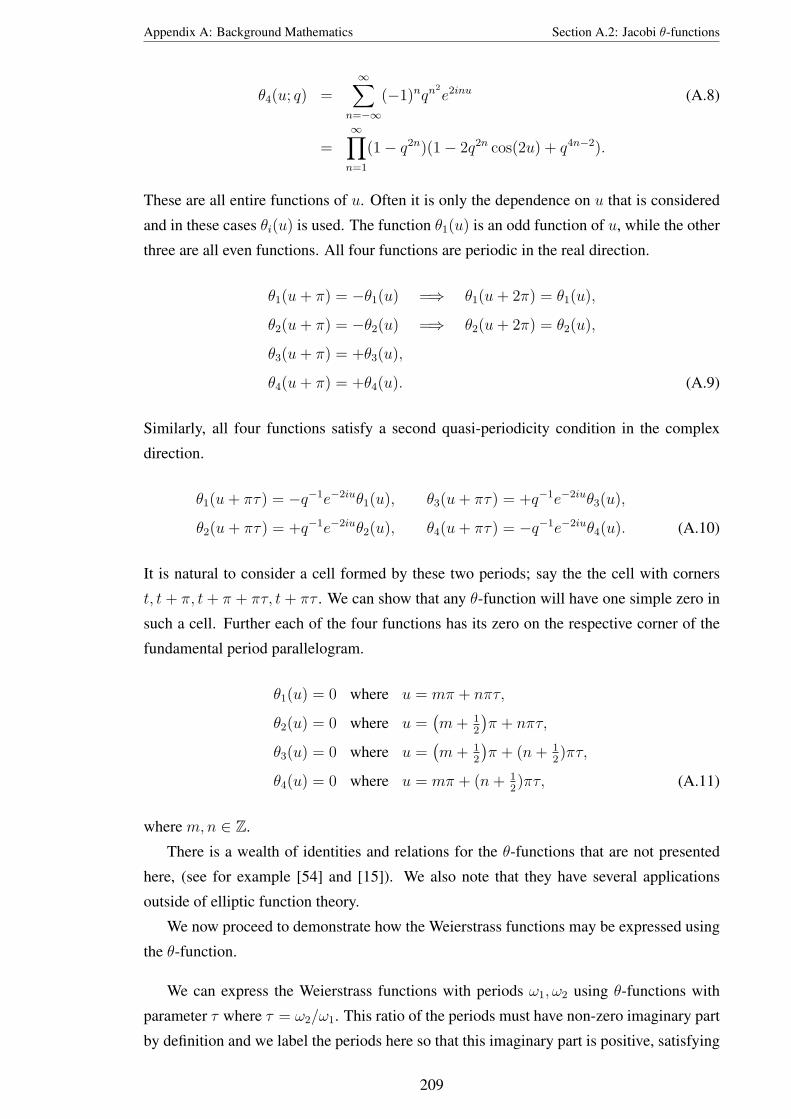
Appendix A: Background Mathematics Section A.2: Jacobi θ-functions
θ4(u; q) =∞∑
n=−∞
(−1)nqn2
e2inu (A.8)
=∞∏n=1
(1− q2n)(1− 2q2n cos(2u) + q4n−2).
These are all entire functions of u. Often it is only the dependence on u that is considered
and in these cases θi(u) is used. The function θ1(u) is an odd function of u, while the other
three are all even functions. All four functions are periodic in the real direction.
θ1(u+ π) = −θ1(u) =⇒ θ1(u+ 2π) = θ1(u),
θ2(u+ π) = −θ2(u) =⇒ θ2(u+ 2π) = θ2(u),
θ3(u+ π) = +θ3(u),
θ4(u+ π) = +θ4(u). (A.9)
Similarly, all four functions satisfy a second quasi-periodicity condition in the complex
direction.
θ1(u+ πτ) = −q−1e−2iuθ1(u), θ3(u+ πτ) = +q−1e−2iuθ3(u),
θ2(u+ πτ) = +q−1e−2iuθ2(u), θ4(u+ πτ) = −q−1e−2iuθ4(u). (A.10)
It is natural to consider a cell formed by these two periods; say the the cell with corners
t, t+ π, t+ π + πτ, t+ πτ . We can show that any θ-function will have one simple zero in
such a cell. Further each of the four functions has its zero on the respective corner of the
fundamental period parallelogram.
θ1(u) = 0 where u = mπ + nπτ,
θ2(u) = 0 where u =(m+ 1
2
)π + nπτ,
θ3(u) = 0 where u =(m+ 1
2
)π + (n+ 1
2)πτ,
θ4(u) = 0 where u = mπ + (n+ 12)πτ, (A.11)
where m,n ∈ Z.
There is a wealth of identities and relations for the θ-functions that are not presented
here, (see for example [54] and [15]). We also note that they have several applications
outside of elliptic function theory.
We now proceed to demonstrate how the Weierstrass functions may be expressed using
the θ-function.
We can express the Weierstrass functions with periods ω1, ω2 using θ-functions with
parameter τ where τ = ω2/ω1. This ratio of the periods must have non-zero imaginary part
by definition and we label the periods here so that this imaginary part is positive, satisfying
209

Appendix A: Background Mathematics Section A.3: Multivariate θ-functions
the assumption on τ . The Weierstrass σ-function can then be expressed as,
σ(u, ω1, ω2) =ω1
πθ′1(0)exp
(− π2
6ω21
θ′′′1 (0)
θ′1(0)u2
)θ1
(πu
ω1
;ω2
ω1
), (A.12)
where the prime notation indicates derivatives with respect to the variable u. Similarly the
Weierstrass ℘-function can be expressed as,
℘(u) =
(π
ω1
)2 [1
3
θ′′′1 (0)
θ′1(0)− d2
dz2
(log[θ1(z; τ)
])], (A.13)
where z = πu/ω1 and τ = ω2/ω1.
A.3 Multivariate θ-functions
The multivariate θ-functions are generalisations of the Jacobi θ-functions discussed in Ap-
pendix A.2. They were first studied by Riemann and are used in this document to realise
the Kleinian σ-function. We give here the definitions and essential information but refer the
reader to [59], [42] and [53] for a detailed study. Note that these functions have applications
outside of Abelian function theory, see for example [16].
Let u ∈ Cg be a vector of variables, m an arbitrary integer column vector and τ a
symmetric matrix with positive definite imaginary part. (This plays a similar role to the
complex number τ in the case of Jacobi θ-functions.)
Definition A.3.1. The canonical θ-function is
θ(u; τ) =∑m∈Zg
exp[2πi(
12mT τm+mTu
) ]. (A.14)
The condition on τ ensures this series converges. As in the classic case this is an even func-
tion of u which satisfies a periodicity condition in the real direction and a quasi-periodicity
condition in the complex direction.
θ(u+ n; τ) = θ(u; τ) ∀n ∈ Zg.
θ(u+ τn; τ) = exp[− 2πi
12nT τn+ uTn
]θ(u; τ) ∀n ∈ Zg. (A.15)
As in the classic case we can define a set of additional θ-functions.
Definition A.3.2. Define a characteristic [ε] as a column vector
[ε] =
[ε′
ε′′
]∈ R2g,
which we split into the two column vectors of length g denoted by ε′ and ε′′.
210

Appendix A: Background Mathematics Section A.3: Multivariate θ-functions
Then the θ-function with characteristic [ε] is given by
θ[ε](u; τ) =∑m∈Zg
exp[2πi
12(m+ ε′)T τ(m+ ε′) + (m+ ε′)T (u+ ε′′)
]. (A.16)
The θ-functions with characteristic can be expressed in terms of the canonical θ-function,
θ[ε](u; τ) = exp[2πi(ε′)T (1
2τε′ + u+ ε′′)
]θ(u+ ε′′ + τε′; τ),
and satisfies similar periodicity properties.
θ[ε](u+ n1 + n2τ ; τ) = exp[− 2πi
nT2u+ 1
2nT2 τn2
− nT1ε′ + nT2ε′′] · θ(u; τ), n1,n2 ∈ Zg.
It is often assumed that the characteristic [ε] is a vector of half integers. Given this property
the θ-functions with characteristic have definite parity.
θ[ε](−u; τ) =
+θ[ε](u; τ) if 4(ε′′)Tε′ ≡ 0 (mod 2)
−θ[ε](u; τ) if 4(ε′′)Tε′ ≡ 1 (mod 2)
We now consider those θ-functions connected to the (n, s)-curveC by setting the matrix
τ = (ω′)−1ω′′ where ω′, ω′′ are the period matrices defined in equation (2.46). Earlier we
noted that (ω′)−1ω′′ does satisfy the condition on τ .
Let ta be some base point on the curve. The branching points of C are connected with
the half-integer characteristics. For a branching point aj the vector,∫ aj
ta
dv = ε′′ + τε′,
where ε′, ε′′ constitute a half-integer characteristic [ε].
We now discuss how to define a special θ-function that vanishes on a particular subset
of the Jacobian of C. It is this function that is used to construct the Kleinian σ-function.
Definition A.3.3. Define
dv = (ω′)−1du (A.17)
to be the basis of normalised holomorphic differentials.
Definition A.3.4. Denote the vector of Riemann constants with base point ta by ∆ta and
define it as below.
(∆ta
)i
=1
2(1 + τii)−
g∑j=1
j 6=i
(∮αj
dvj
∫ t
ta
dvi
), i = 1, . . . , g. (A.18)
211

Appendix A: Background Mathematics Section A.3: Multivariate θ-functions
Here the subscripts indicate the components of the vector and matrices. The vector of
Riemann constants may be expressed as,
∆ta =
ai∑k=1
∫ ai
ta
dv,
where the ai are branching point of the curve. Hence the vector of Riemann constants is
connected to a particular θ-function characteristic [ε] by
∆ta = ω′ε′′ + ω′′ε′.
Definition A.3.5. Define the Riemann θ-function using the canonical θ-function as
R(t) = θ
(∫ t
ta
dv − p−∆ta ; τ
), (A.19)
where t is a point on the curve C and p is a point on the Jacobian J .
Theorem A.3.6. [Riemann’s vanishing theorem]
The Riemann θ-function defined above either vanishes identically or has exactly g zeros
t1, . . . , tg ∈ C such that
g∑i=1
∫ ti
ta
dvj = pj, j = 1 . . . g, (A.20)
where the pj are the components of the point p. The points ti are defined uniquely up to
permutation and are not congruent on the lattice, Λ.
Corollary A.3.7. Define the Theta divisor as the set
Θ =
u ∈ J : u =
g−1∑i=1
∫ ti
ta
du
. (A.21)
Then
θ((ω)−1u−∆ta
)= 0 ∀u ∈ Θ. (A.22)
It is beneficial to set the base point ta to be the point∞ on the curve C. Note that the
Theta divisor then becomes the strata Θ[g−1] from Definition 2.2.14. Denote by ∆∞ the
vector of Riemann constants with base point∞ and let
[δ] =
[δ′
δ′′
]
be the θ-function characteristic that is related to ∆∞.
212

Appendix A: Background Mathematics Section A.4: The Weierstrass Gap Sequence
A.4 The Weierstrass Gap Sequence
The Weierstrass gap sequence was presented in Definition 2.2.3 as follows.
Definition. Let (n, s) be a pair of coprime integers such that s > n ≥ 2. Then the natural
numbers not representable in the form
an+ bs where a, b ∈ N = 0, 1, 2, . . . (A.23)
form a Weierstrass Sequence, Wn,s. The numbers in the sequence are the gaps, with the
numbers representable in the form of equation (A.23) the non-gaps.
In this Appendix we prove some of the properties of the Weierstrass gap sequence.
Lemma A.4.1. Any element of the Weierstrass sequence w ∈ Wn,s can be represented in
the form
w = −αn+ βs where α, β ∈ Z, α > 0, 0 < β < n. (A.24)
The integers α, β are determined uniquely.
Proof. Bezout’s identity tells us that for two non-zero integers, a, b there will exist x, y ∈ Zsuch that xa+ yb = gcd(a, b). Therefore here we have xn+ ys = gcd(n, s) = 1 for some
x, y ∈ Z. Let w be an element of Wn,s. Then
w = (wx)n+ (wy)s
= (wx+ κs)n+ (wy − κn)s
where κ can be any integer. Choose κ such that (wy − κn) ∈ (0, n) — there will be one
unique choice of κ that achieves this. Since this chosen κ ensures the coefficient of s is
positive, the coefficient of n must be negative (or else w /∈ Wn,s by definition). Also, since
the choice of κ was unique the coefficient of n is also unique.
Lemma A.4.2. A Weierstrass sequence Wn,s = w1, w2, . . . , wg has the following prop-
erties
(1) The length of the sequence is g = 12(n− 1)(s− 1).
(2) The maximal element wg is equal to 2g − 1.
(3) If w ∈ Wn,s then (wg − w) /∈ Wn,s.
(4) If w > w where w ∈ Wn,s and w /∈ Wn,s, then (w − w) ∈ Wn,s.
(5) Each element in the gap sequence satisfies i ≤ wi ≤ 2i− 1.
213

Appendix A: Background Mathematics Section A.4: The Weierstrass Gap Sequence
We prove this lemma below. First note that we usually denote the sequence of non-gaps by
W n,s and write both sequences in ascending order.
Wn,s = w1, w2, . . . , wg W n,s = w1, w2, . . .
Example A.4.3. to calculate W3,4 we take each natural number in turn and see if it can be
represented as 3a + 4b for a, b ∈ N. If so it is a nongap and we overline it. We stop once
we have found g = 12(n− 1)(s− 1) = 3 gaps.
0, 1, 2, 3, 4, 5, 6, 7, 8, 9, 10, . . .
So W3,4 = 1, 2, 5.
Proof of Lemma A.4.2
(1) We want to find how many integers there are of the form (A.24). Now, we know that
β ∈ 1, . . . , n − 1, α > 0 and −αn + βs = w > 0. If we set β = l then we know
that α ≤ bls/nc since if it were any greater we would have w < 0. So α ranges over
1, . . . , bls/nc meaning for each possible β there are bls/nc possible α. Hence the
length of the sequence will be
g =n−1∑l=1
⌊ls
n
⌋We can then use Lemma A.4.4 below to conclude g = 1
2(n− 1)(s− 1).
Lemma A.4.4. Let p, q be two coprime integers. Then
q−1∑i=1
⌊ip
q
⌋=
⌊p
q
⌋+
⌊2p
q
⌋+ · · ·+
⌊(q − 1)p
q
⌋=
(p− 1)(q − 1)
2
Proof. Consider a system of Cartesian coordinates. Draw the line connecting the origin
to the point (p, q). Note that since (p, q) are coprime this line contains no other points
with integer coordinates.
The number of points inside the rectangle [(0, 0)→ (0, p)→ (p, q)→ (q, 0)→ (0, 0)]
is clearly (p− 1)(q − 1). The equation of the diagonal line will be y = (p/q)x. Figure
A.1 below gives an example for p = 7, q = 16.
Now consider an integer m. The point mp/q will be the point on the diagonal line
where x = m. The value of bmp/qc will be the number of integer points below that
point. For example, in the diagram we see that when m = 8 there are three such points;
(8,1), (8,2) and (8,3). This corresponds to b8 · 7/16c = b3.5c = 3.
214

Appendix A: Background Mathematics Section A.4: The Weierstrass Gap Sequence
Figure A.1: Example of Lemma A.4.4 with p = 7, q = 16.
Therefore the left hand side of the equality above will be the number of points below
the diagonal line. Now since no integer points lay on the diagonal line, and the total
number of points is (p − 1)(q − 1) we have that exactly half lie below, and so the left
hand side is equal to (p− 1)(q − 1)/2.
(2) First note that
2g − 1 = (n− 1)(s− 1)− 1 = ns− n− s
= s(n− 1)− n.
So by Lemma A.4.1 we know that 2g− 1 is in the gap sequence. Suppose for a contra-
diction that there exists another number w of the form (A.24) that is greater than 2g−1.
Then we have α, β such that
−αn+ βs > −n+ s(n− 1) =⇒ α < 1− sn(n− 1− β).
We know that α ≥ 1, which means that −sn(n − 1 − β) > 0. Since n and s are both
positive we must have,
n− 1− β < 0 =⇒ β > n− 1 =⇒ β ≥ n,
which is a contradiction.
(3) From part (2) we have that wg = 2g − 1 = −n+ s(n− 1). Therefore, for some α, β
wg − w = −n+ s(n− 1)− (−αn+ βs) = (α− 1)n+ (n− 1− β)s.
Therefore (wg−w) can be expressed in the form of (A.23) and hence (wg−w) /∈ Wn,s.
215

Appendix A: Background Mathematics Section A.4: The Weierstrass Gap Sequence
(4) Let w ∈ Wn,s and w /∈ Wn,s. Therefore
w = −αn+ βs, w = an+ bs.
Then
w − w = −αn+ βs− (an+ bs) = −(α + a)n+ (β − b)s > 0.
(The> 0 was by assumption in the statement.) Now we can check that (w−w) ∈ Wn,s.
Clearly (α+ a) > 0 and since (w−w) > 0 we have (β − b) > 0. Finally, since β < n
we also have (β − b) < n which shows (w − w) to be of the form (A.24).
(5) Consider the set,
Wn,s = 2g − 1− wg+1−ii=1,...,g = (wg − wg), (wg − wg−1), . . . , (wg − w1),
recalling that wg = 2g−1 from part (2). Next, by part (3), we know that Wn,s∩Wn,s =
φ. Then, since both Wn,s and Wn,s contain g elements, we have that Wn,s ∪ Wn,s
contains 2g different non-negative integers, each of which is less than 2g − 1. Hence
Wn,s ∪Wn,s is a permutation of
0, 1, 2, . . . , (2g − 1).
Now let N(L) be the number of integers of the form (A.23) that are less than L. Then
w1, . . . , wN(wi) ⊂ Wn,s, w1, . . . , wi ⊂ Wn,s
and the intersection w1, . . . , wN(wi)∩w1, . . . , wi is therefore empty. Similarly, the
union w1, . . . , wN(wi) ∪ w1, . . . , wi will be permutation of the set 0, 1, 2, . . . , wifor any wi ∈ Wn,s. Now, in this case 2g = i+N(wi) and hence wi = i+N(wi)− 1.
Next note that w0 = 0 < wi and so N(wi) ≥ 1. Then by the definition of N(wi) we
see that wi ≥ i for all wi ∈ Wn,s.
Next, by part (4) we have that
(wi − w1), (w2 − w2) . . . , (wi − wN(wi)) ⊂ w1, . . . , wi
and so N(wi) ≤ i. Thus
wi = i+N(wi)− 1 ≤ 2i− 1.
So, as required, we have i ≤ wi ≤ 2i− 1 for all i = 1, . . . , g.
216

Appendix A: Background Mathematics Section A.5: The Schur-Weierstrass polynomial
A.5 The Schur-Weierstrass polynomial
In this Appendix we define and construct Schur Weierstrass polynomials. The material here
loosely follows [20] with extra material cited independently when used. These polynomials
will be defined by a pair of coprime integers (n, s) and use results on the Weierstrass gap
sequence that were discussed in the previous Appendix. Schur-Weierstrass polynomials
are important in this document as they form the first part of the series expansion about the
origin of the Kleinian σ-function associated with the corresponding (n, s)-curve.
A.5.1 Weierstrass Partitions
Definition A.5.1. A partition, π of length m is a non-increasing set of m positive integers
πi written π = π1, . . . , πm.
For example, 3, 2, 2, 2, 1 is a partition of length 5. Let Parm denote the set of all partitions
of length m and let the symbol # denote the operation of taking the cardinality (number of
elements) of a set.
Definition A.5.2. We define the following conjugation operation on the set of partitions
and denote it using the dash symbol.
π′ = π1, . . . , πm′def= π′1, . . . , π′m′ where π′i = #j : πj ≥ i and m′ = π1.
Note that π′′ = π.
Example A.5.3. We apply the operation on the partition π = 3, 2, 2, 2, 1. In this case
m′ = π1 = 3. The elements of the new set will be
π′1 = #j : πj ≥ 1 = #π = 5, π′2 = #j : πj ≥ 2 = 4, π′3 = #j : πj ≥ 3 = 1.
So π′ = 5, 4, 1. Similarly we can check that π′′ = π.
Let WSg denote the set of all Weierstrass gap sequences of length g.
Lemma A.5.4. Let Wn,s = w1, . . . , wg be a Weierstrass gap sequence. Then the map
χ(Wn,s) = π where πk = wg−k+1 + k − g, k = 1, . . . , g (A.25)
defines an embedding χ : WSg → Parg.
Proof. We need to show that χ(Wn,s) is a partition as defined above. (I.e. show that the
πi are all positive, non increasing integers.) Clearly all the πj are integers. We have that
217

Appendix A: Background Mathematics Section A.5: The Schur-Weierstrass polynomial
wi − 1 ≥ 0 for all i = 1, . . . , g from Lemma A.4.2(5). Now, for j = 1, . . . , g we find that
i = g + 1− j is an integer within [1, . . . , g]. Therefore
wg+1−j − g − 1 + j ≥ 0
wg+1−j − g + j > 0 =⇒ πj > 0 j = 1, . . . , g
It remains to show that the πk are non increasing. Consider
πk − πk+1 = [wg−k+1 + k − g]− [wg−(k+1)+1 + (k + 1)− g] = wg−k+1 − wg−k − 1
Now Wn,s is a strictly increasing sequence by definition so πk − πk+1 ≥ 1 − 1 = 0, and
hence the the πk are non increasing as required.
Definition A.5.5. A partition π that is the image of a Weierstrass gap sequence under the
mapping χ is defined to be a Weierstrass Partition, denoted by
πn,s = χ(Wn,s).
Example A.5.6. In equation (3.3) we derived W4,5 = 1, 2, 3, 6, 7, 11. Hence
π4,5 = χ(W4,5) = w6 − 5, w5 − 4, w4 − 3, w3 − 2, w2 − 1, w1 = 6, 3, 3, 1, 1, 1
Lemma A.5.7. Weierstrass Partitions have the following properties.
(1) π′n,s = πn,s.
(2) π1 = g, πg = 1 and πn,s ⊂ g, g − 1, . . . , 1.c
Example A.5.8. In Example A.5.6 we derived π4,5. A quick check will show that, as
predicted by Lemma A.5.7, we have π′4,5 = 6, 3, 3, 1, 1, 1 = π4,5. Also we can check that
π1 = g = 6 and πg = π6 = 1.
For the proof of Lemma A.5.7 we require the following theorem.
Theorem A.5.9. For any partition µ ∈Parn such that µ1 = m, the set consisting of the
m+ n numbers,
µi + n− 1 (1 ≤ i ≤ n) n− 1 + j − µ′j (1 ≤ j ≤ m),
is a permutation of the set 0, 1, 2, . . . , (m+ n− 1).
218

Appendix A: Background Mathematics Section A.5: The Schur-Weierstrass polynomial
Proof. (We follow [56] page 3.) Let µ ∈ Parn and µ1 = m. Note that we have µ′1 = n.
First, draw the Young diagram induced by the partition. This will consist of rows of cubes,
with the first row containing µ1 cubes, the second µ2 etc. Figure A.2 contains the Young
diagram for the partition 5, 4, 4, 1.
Figure A.2: The Young diagram forthe partition 5, 4, 4, 1 is given by theshaded squares. We have n = 4 andm = 5.
Such a diagram will be contained within a rectangle of m × n cubes as in Figure A.2.
We separate the diagram from its complement inside the rectangle, by highlighting the line
segments between the two sets. There will clearly be (n + m) line segments that separate
the diagram of µ from its complement within the rectangle. Label these line segments
0, 1, 2, . . . , (m + n − 1), starting at the bottom left hand corner. (See Figure A.2 for
example). We find that the numbers attached to the vertical line segments are, starting from
the top left, given by
µj + n− i (1 ≤ i ≤ n).
This is because at each vertical segment you will have already traveled µi segments across
and (n− i) segments up. We then see the numbers attached to the horizontal segments are,
starting from the bottom right,
(m+ n− 1)− (µ′j +m− j) = n− 1 + j − µ′j (1 ≤ j ≤ m).
This is because, before you travel along a horizontal segment, you will have traveled the
total (m + n − 1), minus the number of rows left (µ′j) and minus the number of columns
not yet considered, (m− j).
So, we have shown that the n + m numbers described by the two equations above will
correspond to the n + m line segments in the diagram. Hence these are a permutation of
the set 0, 1, 2, . . . , (m+ n− 1).
Example A.5.10. We demonstrate the main argument in the proof of Theorem A.5.9 for
the partition 5, 4, 4, 1, with Young diagram given in Figure A.2. Here
µ1 = 5, µ2 = 4, µ3 = 4, µ4 = 1, m = 5,
µ′1 = 4, µ′2 = 3, µ′3 = 3, µ′4 = 3, µ′5 = 1 n = 4.
219

Appendix A: Background Mathematics Section A.5: The Schur-Weierstrass polynomial
So the vertical line segments should be given (from top to bottom) by
µj + n− i (1 ≤ i ≤ n) =⇒ µj + 4− i (1 ≤ i ≤ 4).
i = 1 =⇒ 5 + 4− 1 = 8, i = 3 =⇒ 4 + 4− 3 = 5,
i = 2 =⇒ 4 + 4− 2 = 6, i = 4 =⇒ 1 + 4− 4 = 1.
While the horizontal line segments should be given (from bottom to top) by
n− 1 + j − µ′j (1 ≤ j ≤ m) =⇒ 4− 1 + j − µ′j (1 ≤ j ≤ 5).
j = 1 =⇒ 3 + 1− 4 = 0, j = 4 =⇒ 3 + 4− 3 = 4,
j = 2 =⇒ 3 + 2− 3 = 2, j = 5 =⇒ 3 + 5− 1 = 7.
j = 3 =⇒ 3 + 3− 3 = 3,
As expected, these match the labels in Figure A.2.
We can now prove Lemma A.5.7.
Proof. [Lemma A.5.7] We will apply Theorem A.5.9 to πn,s. It has length g, and, from
equation (A.25) we see
π1 = wg + 1− g = (2g − 1) + 1− g = g.
Therefore, the set of 2g numbers
πi + g − 1 = wg+1−i i = 1, . . . , g
g − 1 + j − π′j = (2g − 1)− (π′j + g − j) j = 1, . . . , g
is a permutation of the set 0, 1, 2, . . . , (2g− 1). This implies that the set 2g− 1− (π′j +
g−1)j=1,...,g is the complement of the sequenceWn,s within the set 0, 1, 2, . . . , (2g−1).However, from Lemma A.4.2(3) we know that this complement can be expressed as
wg − wii=1,...,g = wg − wg+1−jj=1,...,g = (2g − 1)− wg+1−j.
It then follows that
π′j = wg+1−j + j − g = πj (1 ≤ j ≤ g),
which completes the proof of Lemma A.5.7(1).
To prove part (2) we need to show that πk ∈ 1, . . . , g for k = 1, . . . , g. So we must
prove that, for k = 1, . . . , g
1 ≤ πk ≤ g
1 ≤ wg−k+1 + k − g ≤ g
220

Appendix A: Background Mathematics Section A.5: The Schur-Weierstrass polynomial
g − k + 1 ≤ wg−k+1 ≤ 2g − 1
g − k + 1 ≤ wg−k+1 ≤ g + (g − k + 1)− 1
Now we make the substitution j = (g− k+ 1) =⇒ g = j+ k− 1 into the above inequality
(j will run from g to 1). So now we must show that
j ≤ wj ≤ (j + k − 1) + (j)− 1
j ≤ wj ≤ (2j − 1) + (k − 1)
Finally, we note that (k − 1) ≥ 0 so it would satisfy to show that
j ≤ wj ≤ 2j − 1 j = 1, . . . , g.
This is the case by Lemma A.4.2 (5).
A.5.2 Symmetric polynomials
We now need some preliminary results on symmetric polynomials. For more detailed in-
formation on these polynomials see [56] Section 1.2 for example.
Definition A.5.11. A symmetric polynomial in n variables x1, . . . , xn is a function that
is unchanged by any permutation of its variables. Therefore symmetric polynomials satisfy
f(y1, y2, . . . , yn) = f(x1, x2, . . . , xn),
where yi = xπi and π = πii=1,...,n is an arbitrary permutation of the indices 1, 2, . . . , n.
We now define a class of symmetric polynomials from which all other symmetric poly-
nomials may be defined
Definition A.5.12. The elementary symmetric polynomials in m variables are defined by
er(x1, x2, . . . , xm) =∑
1≤j1<j2<···<jr≤m
xj1 . . . xjr r = 0, 1, 2, . . . ,m.
So we have
e0(x1, x2, . . . , xm) = 1
e1(x1, x2, . . . , xm) =∑
1≤j≤m
xj
e2(x1, x2, . . . , xm) =∑
1≤j1<j2≤m
xj1xj2
...
em(x1, x2, . . . , xm) = x1x2 · · ·xm
221

Appendix A: Background Mathematics Section A.5: The Schur-Weierstrass polynomial
These can be introduced by means of the generating function below. Here the coefficient of
tr in the expansion on the right hand side will be the rth elementary symmetric polynomial
in m variables.
Em(t) =m∑r=0
ertr =
m∏i=1
(1 + xit).
The elementary symmetric polynomials form a basis for the space of all symmetric poly-
nomials.
The elementary Newton polynomials
Definition A.5.13. The elementary Newton polynomials in m variables are
pr(x1, . . . , xn) = xr1 + · · ·+ xrm =m∑i=1
xri .
These can be introduced by means of the generating function below.
P (t) =∑r≥1
prtr−1 =
∑i≥1
xi(1− xit)
. (A.26)
The functions pr are algebraically independent over Q, the field of rational numbers.
Theorem A.5.14. The elementary symmetric polynomials may be expressed using elemen-
tary Newton polynomials using the following determinant expression.
ek =1
k!
∣∣∣∣∣∣∣∣∣∣∣∣∣∣∣∣∣∣
p1 1 0 . . . 0 0 0
p2 p1 2 . . . 0 0 0
p3 p2 p1 . . . 0 0 0...
...... . . . ...
......
pk−2 pk−3 pk−4 . . . p1 k − 2 0
pk−1 pk−2 pk−3 . . . p2 p1 k − 1
pk pk−1 pk−2 . . . p3 p2 p1
∣∣∣∣∣∣∣∣∣∣∣∣∣∣∣∣∣∣. (A.27)
The generating functions are related by the formula P (−t)E(t) = E ′(t).
Proof. See [56] page 28.
Example A.5.15. We calculate e3 in m = 3 variables using equation (A.27).
e3 =1
6
∣∣∣∣∣∣∣∣p1 1 0
p2 p1 2
p3 p2 p1
∣∣∣∣∣∣∣∣6e3 = p1(p2
1 − 2p2)− (p1p2 − 2p3) = p31 − 3p1p2 + 2p3
222

Appendix A: Background Mathematics Section A.5: The Schur-Weierstrass polynomial
Now, in 3 variables the elementary Newton polynomials are
p1 = x1 + x2 + x3, p2 = x21 + x2
2 + x23, p3 = x3
1 + x32 + x3
3.
So, multiplying out and canceling we find
6e3 = p31 − 3p1p2 + 2p3 = 6x1x2x3
So, with 3 variables, e3 = x1x2x3, as expected.
A.5.3 Schur-Weierstrass Polynomials
Schur polynomials are defined using a partition as follows.
Definition A.5.16. Given a partition of length n,
π = π1, π2, · · · , πn
the corresponding Schur polynomial of n variables is
sπ(x1, x2, . . . xn) =
det
xπ1+n−1
1 xπ1+n−12 . . . xπ1+n−1
n
xπ2+n−21 xπ2+n−2
2 . . . xπ2+n−2n
...... . . . ...
xπn1 xπn2 . . . xπnn
det
xn−1
1 xn−12 . . . xn−1
n
xn−21 xn−2
2 . . . xn−2n
...... . . . ...
1 1 . . . 1
=det(xπi+n−ij )1≤i,j≤n
det(xn−1j )1≤i,j≤n
.
The denominator is a Vandermonte determinant and so
det
xn−1
1 xn−12 . . . xn−1
n
xn−21 xn−2
2 . . . xn−2n
...... . . . ...
1 1 . . . 1
=∏
1≤j<k≤n
(xj − xk).
The numerator will be divisible by each factor (xj−xk) and so sπ is a polynomial. Further,
since both the numerator and denominator are determinants, both will change sign under
223

Appendix A: Background Mathematics Section A.5: The Schur-Weierstrass polynomial
any transposition of the variables. These sign changes will cancel each other out and hence
the Schur polynomial itself is a symmetric polynomial.
Theorem A.5.17. A Schur polynomial, sπ corresponding to an arbitrary partition π of
length m can be represented using elementary symmetric polynomials as
sπ = det((eπ′i−i+j)1≤i,j≤m
). (A.28)
Proof. See [56] page 40.
Definition A.5.18. Denote by Sn,s the Schur polynomial corresponding to a Weierstrass
partition πn,s.
Given such a Schur polynomial we have case m = g and π′i = πi and so equation (A.28)
becomes
Sn,s = det((eπi−i+j)1≤i,j≤g
)
=
∣∣∣∣∣∣∣∣∣∣∣∣∣∣∣∣∣∣∣
eπ1 eπ1+1 eπ1+2 . . . eπ1+λ−1 . . . eπ1+g−1
eπ2−1 eπ2 eπ2+1 . . . eπ2+λ−2 . . . eπ2+g−2
eπ3−2 eπ3−1 eπ3 . . . eπ3+λ−3 . . . eπ3+g−3
......
... . . . ......
eπλ−λ+1 eπλ−λ+2 eπλ−λ+3 . . . eπλ . . . eπλ+g−λ...
......
... . . . ...
eπg−g+1 eπg−g+2 eπg−g+3 . . . eπg+−g+λ . . . eπg
∣∣∣∣∣∣∣∣∣∣∣∣∣∣∣∣∣∣∣
. (A.29)
Now recall that πn,s ⊂ g, . . . , 1 with π1 = g and πg = 1. Therefore, the largest subscript
will be π1 + g − 1 = 2g − 1. The smallest subscript will actually be πg − g + 1 = −ghowever, by convention we set ek to 0 for k < 0. Hence
Sn,s = Sn,s(e1, . . . , e2g−1).
Theorem A.5.19. Using equation (A.27) we can represent Sn,s via the elementary Newton
polynomials pi. When using this representation Sn,s will be a polynomial in g variables
pw1 , . . . , pwg where w1, . . . , wg = Wn,s.
Proof. See [20] Theorem 4.1.
Therefore, given a polynomial Sn,s, it may be represented using Theorem A.5.19 as
Sn,s(pw1 , . . . , pwg).
224

Appendix A: Background Mathematics Section A.5: The Schur-Weierstrass polynomial
Definition A.5.20. We define the Schur-Weierstrass polynomial associated with (n, s) as
follows. First form the Schur polynomial generated by (n, s) as a function of elementary
Newton polynomials,
Sn,s(pw1 , . . . , pwg).
We then find the Schur-Weierstrass polynomial by applying the change of variables
pwi = wiug+1−i, i = 1, . . . , g
and denote this polynomial by SWn,s.
SWn,s = Sn,s(wgug, . . . , w1u1).
Summary
To calculate the Schur-Weierstrass polynomial generated by (n, s):
(1) Calculate the Weierstrass Sequence Wn,s of length g = 12(n− 1)(s− 1).
(2) Calculate the corresponding Weierstrass partition πn,s.
(3) Define the elementary symmetric polynomials
ek, k = 1, . . . , (2g − 1)
in terms of the elementary Newton polynomials pi using equation (A.27).
(4) Calculate Sn,s as the determinant in equation (A.29). By Theorem A.5.19 this is a
polynomial in g variables, pw1 , . . . , pwg.
(5) Find the Schur-Weierstrass polynomial by making the change of variables
pwi = wiug+1−i i = 1, . . . , g.
Example A.5.21. We now construct the Schur-Weierstrass polynomial associated with the
(4,5)-curve. In equation (3.3) we calculated the gap sequence, SW4,5 = 1, 2, 3, 6, 7, 11.Then in Example A.5.6 the associated Weierstrass partition was calculated as
π4,5 = 6, 3, 3, 1, 1, 1.
Substitute the values of π4,5 into equation (A.29). Recall that e0 = 1 and that ek is zero for
225

Appendix A: Background Mathematics Section A.5: The Schur-Weierstrass polynomial
negative k to find
S4,5 =
∣∣∣∣∣∣∣∣∣∣∣∣∣∣∣∣
e6 e7 e8 e9 e10 e11
e2 e3 e4 e5 e6 e7
e1 e2 e3 e4 e5 e6
0 0 1 e1 1 0
0 0 0 0 e1 1
0 0 0 0 1 e1
∣∣∣∣∣∣∣∣∣∣∣∣∣∣∣∣.
Now use equation (A.27) to describe the elementary symmetric polynomials using New-
ton polynomials.
e1 =1
1!|1| = 1, e2 =
1
2!
∣∣∣∣∣p1 1
p2 p1
∣∣∣∣∣ =p2
1 − p2
2,
e3 =1
3!
∣∣∣∣∣∣∣∣p1 1 0
p2 p1 2
p3 p2 p1
∣∣∣∣∣∣∣∣ =1
6
(p1(p2
1 − 2p2)− (p1p2 − 2p3)
)=p3
1
6− p1p2
2+p3
3.
Using Maple, we find similarly that
e4 = 124p4
1 − 14p2p
21 + 1
3p3p1 + 1
8p2
2 − 14p4,
e5 = 1120p5
1 − 112p2p
31 + 1
6p3p
21 + 1
8p1p
22 − 1
4p4p1 − 1
6p2p3 + 1
5p5,
e6 = 1720p1
6 − 148p2p1
4 + 118p3p1
3 + 1148
16p12p2
2 − 18p4p1
2 − 16p3p1p2
− 1148
48p23 + 1
8p4p2 + 1
18p3
2 + 15p5p1 − 1
6p6,
e7 = − 112p1
2p2p3 + 18p4p1p2 + 1
24p2
2p3 − 110p5p2 − 1
12p3p4 + 1
5040p1
7 + 17p7 − 1
6p6p1
− 1240p1
5p2 + 172p1
4p3 + 148p1
3p22 − 1
24p4p1
3 + 110p5p1
2 − 148p1p2
3 + 118p3
2p1,
e8 = 116p1
2p2p4 − 136p1
3p2p3 − 136p2p3
2 − 132p2
2p4 − 110p5p1p2 + 1
24p1p2
2p3 + 11127p7p1
+ 115p3p5 − 1
12p3p1p4 + 1
12p6p2 + 1
32p4
2 + 1384p2
4 − 112p6p1
2 + 136p1
2p32 − 1
8p8
− 196p1
2p23 + 1
30p5p1
3 − 196p4p1
4 + 1192p2
2p14 + 1
360p3p1
5 − 11440
p16p2 + 1
40320p1
8,
e9 = − 124p1
2p3p4 + 19p9 + 1
24p2p3p4 − 1
36p6p1
3 + 114p7p1
2 − 114p7p2 − 1
8p8p1
+ 112p6p1p2 + 1
48p1
3p2p4 − 120p1
2p2p5 − 1144p2
3p3 + 140p2
2p5 + 12160
p16p3
− 110080
p17p2 + 1
384p1p2
4 − 1480p1
5p4 + 1162p3
3 + 132p1p4
2 + 148p1
2p22p3 − 1
18p3p6
+ 1362880
p19 + 1
960p1
5p22 + 1
108p1
3p32 − 1
288p1
3p23 + 1
120p1
4p5 − 132p1p2
2p4
− 136p2p1p3
2 − 120p4p5 − 1
144p1
4p2p3 + 115p3p1p5,
e10 = − 1720p2p3p1
5 + 115120
p17p3 + 1
9p9p1 − 1
2880p1
6p4 + 1162p1p3
3 − 110p10
− 164p1
2p22p4 + 1
5760p1
6p22 + 1
42p7p1
3 − 116p8p1
2 + 116p8p2 − 1
14p7p1p2
+ 1600p1
5p5 + 150p5
2 − 1144p1
4p6 + 1432p1
4p32 − 1
1152p1
4p23 + 1
768p1
2p24 + · · ·
226

Appendix A: Background Mathematics Section A.5: The Schur-Weierstrass polynomial
· · ·+ 124p1
2p2p6 − 120p1p4p5 + 1
24p4p6 − 1
72p1
2p2p32 + 1
30p1
2p3p5 − 180640
p18p2
+ 164p1
2p42 − 1
3840p2
5 + 140p1p2
2p5 − 1144p1p2
3p3 + 1192p2
3p4 − 148p2
2p6
+ 1144p2
2p32 − 1
64p2p4
2 + 1192p1
4p2p4 − 160p1
3p2p5 + 1144p1
3p22p3 − 1
72p3
2p4
− 118p3p1p6 + 1
21p3p7 − 1
72p1
3p3p4 + 13628800
p110 − 1
30p2p3p5 + 1
24p2p1p3p4,
e11 = 190p5p3p1
3 − 1240p5p2p1
4 − 1288p4p1
4p3 + 1960p4p1
5p2 − 120160
p4p17 + 1
1152p2
4p3
+ 13600
p5p16 + 1
48p1
2p2p3p4 + 140p2p4p5 − 1
30p2p1p3p5 + 1
36p2p3p6 − 1
30p5p6
− 196p2
2p3p4 + 139916800
p111 − 1
10p10p1 − 1
48p8p1
3 + 118p9p1
2 − 118p9p2 + 1
144p1p2
2p32
+ 1324p1
2p33 − 1
720p1
5p6 + 12160
p15p3
2 − 15760
p15p2
3 + 140320
p17p2
2 + 111p11
+ 1120960
p18p3 − 1
725760p1
9p2 + 1168p1
4p7 + 12304
p13p2
4 + 1192p1
3p42 − 1
240p2
3p5
− 13840
p1p25 + 1
50p1p5
2 + 116p8p1p2 − 1
324p2p3
3 − 172p1p3
2p4 + 190p3
2p5 + 156p2
2p7
+ 196p3p4
2 − 124p3p8 + 1
21p3p1p7 + 1
24p1p4p6 − 1
28p4p7 − 1
64p2p1p4
2 + 1192p1p2
3p4
+ 172p1
3p2p6 − 140p1
2p4p5 − 1216p1
3p2p32 − 1
4320p1
6p2p3 − 1192p1
3p22p4
− 128p1
2p2p7 + 180p1
2p22p5 − 1
288p1
2p23p3 + 1
576p1
4p22p3 − 1
36p1
2p3p6 − 148p1p2
2p6.
The next step is to substitute these into S4,5 and evaluating the determinant. Using Maple
we find that many terms cancel to leave
S4,5 = 14032
p22p1
8p3 − 11512
p2p17p6 + 1
7056p7p1
8 + 1252p7p3p1
5 + 1168p7p2
2p14
− 11944
p33p1
6 − 127216
p19p3
2 + 11197504
p3p112 − 1
12096p2
4p17 − 1
133056p2
2p111
− 144p2
2p11 − 1126p3
2p12p7 + 1
216p3
3p12p2
2 + 133p3p1p11 − 1
108p3p6
2
− 11728
p3p26 − 1
432p3
2p1p24 + 1
336p2
4p7 + 142p6p2p7 + 1
84p3p1p7p2
2 + 1108p1
3p62
− 154p3
2p1p6p2 + 1216p3p2
3p6 − 1216p3p6p2p1
4 + 1972p3
5 − 149p7
2p1 + 1972p3
4p13
− 1132p1
4p11 + 11728
p26p1
3 − 1216p2
3p6p13 − 1
1728p2
4p3p14 + 1
8382528p1
15.
Note that as predicted by Theorem A.5.19, this is a function of g variables, pw1 , . . . , pwg.Finally, by Definition A.5.20, we make the change of variables to give,
SW4,5 = 18382528
u156 + 1
336u8
6u25u4 − 1
12u4
6u1 − 1126u7
6u3u5 − 16u4u3u5u
46 − u5
2u1
− 172u3
4u66 − 1
33264u11
6 u25 + 1
27u6
5u36 + 2
3u4u
35u3 − 2u2
4u6u3u5 − u22u6 + u4u6u1
− 29u3
5u3u36 − u4u
23 + 1
12u4
4u36 − 1
3024u9
6u24 − 1
756u7
6u45 + 1
1008u8
6u2 − 13u4
2u6u54
+ 13u4
5u2 + 13u3
6u23 − 1
9u4u
65 + 1
399168u12
6 u4 + u4u6u25u2 + 1
4u5
4 − 136u5
4u4u64
+ 2u5u3u2 + 16u5
2u64u2 + 1
12u6
5u2u4 − 12u4
2u62u2 + 1
2u4
3u62u5
2.
227

Appendix A: Background Mathematics Section A.6: Resultants
A.6 Resultants
This Appendix will give a short overview of the theory of resultants. For more information
see Chapter 12 of [43]. We use resultants in several parts of this document as a tool to
eliminate variables from equations. In these computations it was implemented using the
standard resultant command in the computer algebra package Maple.
Definition A.6.1. Let p(x) be a polynomial of degree n,
p(x) = anxn + an−1x
n−1 + · · ·+ a1x+ a0, (A.30)
and denote the roots of p(x) by αi where i = 1, . . . , n. Similarly, let q(x) be a polynomial
of degree m,
q(x) = bmxm + bm−1x
m−1 + · · ·+ b1x+ b0, (A.31)
and denote the roots of q(x) by βj where j = 1, . . . ,m. Then the resultant of the polyno-
mials is defined as
Res(p, q) = amn bnm
n∏i=1
m∏j=1
[αi − βj
].
So the resultant of the polynomials is zero if and only if they share a common root. The
resultant may be realised as the determinant of the corresponding Sylvester matrix.
Definition A.6.2. Consider the two polynomials of degrees n and m in equations (A.30)
and (A.31). The corresponding Sylvester matrix is an (m + n) × (m + n) matrix formed
as follows.
Start at the upper left corner and fill the top row with the coefficients of p(x). Repeat
this on the second row, shifting each entry to the right. Continue this process until the
coefficients hit the right hand side. Then repeat the process again using the coefficients of
q(x), starting on the next row down. All other matrix entries are set to zero.
For example, if m = 3 and n = 2 then
Res(p, q) =
∣∣∣∣∣∣∣∣∣∣∣∣∣
a3 a2 a1 a0 0
0 a3 a2 a1 a0
b2 b1 b0 0 0
0 b2 b1 b0 0
0 0 b2 b1 b0
∣∣∣∣∣∣∣∣∣∣∣∣∣.
Note that the resultant does not depend on the variable x.
The resultant can be used to search for solutions to the equations
p(x) = 0, q(x) = 0. (A.32)
228

Appendix A: Background Mathematics Section A.6: Resultants
This is because when the resultant is zero, the polynomials have a common root and hence
equations (A.32) are satisfied.
More generally it may be used to eliminate variables between equations, (the use it is
put to in this document). To do this we write two equations as polynomials that must be
zero, and take the resultant with respect to the variable that we want eliminated. We obtain
a polynomial that does not contain that variable and that when equal to zero implies the
original equations are satisfied.
We demonstrate this with a simple example
Example A.6.3. Suppose we wish to eliminate the variable x1 from the equations
4x1 + x21 + 9x2 = 0
−x21 + 10x2 + 4x3
2 = 0.
The resultant of these equations with respect to x1 is
Res =
∣∣∣∣∣∣∣∣∣∣1 4 9x2 0
0 1 4 9x2
−1 0 10x2 + 4x32 0
0 −1 0 10x2 + 4x32
∣∣∣∣∣∣∣∣∣∣= −160x2 − 64x3
2 + 361x22 + 152x4
2 + 16x62.
Hence we have eliminated x1.
This was a simple example to demonstrate the concept. The resultant approach may
be used in far more complicated circumstance, with polynomials of many variables and a
high degree. In these cases it is an efficient method for eliminating variables. Note that the
Sylvester matrix is not the only method of determining the resultant. If m = n then the
resultants may be computed using a Bezout matrix, (see [43] Chapter 12).
It is possible to define the multivariant result of a group of polynomials in analogy to
Definition A.6.1, however we do not use these in this document. For more information see
[43] Chapter 13.
229
Appendix B
Independence from the constant c
Recall Definition 2.2.15 which defined the Kleinian σ-function using the period matrices
and θ-function characteristic [δ] as
σ(u) = c exp(
12uη′(ω′)−1uT
)×∑m∈Zg
exp
[2πi
12(m+ δ′)T (ω′)−1ω′′(m+ δ′) + (m+ δ′)T ((ω′)−1uT + δ′′)
].
Here c was a constant that depends on the curve parameters and was fixed in Remark 2.2.23
so that K = 1 in Theorem 2.2.21. It was remarked at the time that this choice of c differs
from the choice of some other authors working in this area, and that these choice are not
equivalent in general. However, all the Abelian functions and almost all the results in this
document are independent of the choice of c. This Appendix is dedicated to proving this
fact.
Notation
Note that the constant c does not vary with u and hence may be taken outside of the differ-
entiation when considering σ-derivatives. Hence both the σ-function all the σ-derivatives
may be factored to give c multiplied by an infinite sum that does not vary with c. In this
section, when a function may be factored in this way we denote the part of a function that
does not vary with c with the bar notation. Hence
σ(u) = cσ(u)
σi1,i2,...,in(u) = cσi1,i2,...,in(u)
If a function f(u) is independent of c then f(u) = f(u).
230

Appendix B: Independence from the constant c
Kleinian ℘-functions
Now we will prove that all the Kleinian ℘-functions are independent of c.
Proposition B.0.4. The 2-index ℘-functions are independent of the constant c.
Proof. Recall Definition 2.2.24 for the 2-index ℘-functions. Take the derivatives to obtain
℘ij(u) =σi(u)σj(u)− σ(u)σij(u)
σ(u)2(B.1)
=cσi(u)cσj(u)− cσ(u)cσij(u)
c2σ(u)2=σi(u)σj(u)− σ(u)σij(u)
σ(u)2
= ℘ij(u) (B.2)
Once the definition was expanded it was possible to factor out the constant c to obtain
something independent of c which we label ℘ij(u). Both the numerator and denominator
contained c2 which canceled so we can conclude ℘ij(u) independent of the constant c.
Such a cancellation occurs for all the n-index ℘-functions. We can prove this using the
following lemma.
Lemma B.0.5. An n-index ℘-function can be expressed as
℘i1,i2,...,in(u) =h(u)
σ(u)n,
where h(u) is a finite polynomial in which each term is a product of n functions. These
functions are all either σ(u) or σ-derivatives
σi1,i2,...,im(u), where m ≤ n.
Proof. We will prove this by induction. The statement is clearly true for n = 2 from
equation (B.1). Now assume that the statement holds for a k-index ℘-function:
℘i1,i2,...,ik(u) =h(u)
σ(u)k
where h(u) is a sum of terms, each a product of k m-index σ-derivatives with m ≤ k. Now
differentiate this fraction with respect to ui to obtain a (k + 1)-index ℘-function.
℘i1,i2,...,ik,ik+1(u) =
[σ(u)k
] [ ∂
∂uih(u)
]−[h(u)
][kσ(u)k−1σi(u)
]σ(u)2k
.
We can factor out σ(u)k−1 from the numerator and cancel to leave 2k − (k − 1) = k + 1
231

Appendix B: Independence from the constant c
powers of σ(u) in the denominator.
℘i1,i2,...,ik,ik+1(u) =
σ(u)
[∂
∂uih(u)
]− kh(u)σi(u)
σ(u)k+1. (B.3)
The denominator of equation (B.3) is already in the correct form. Due to the assumption
on h(u) so is the second term in the numerator.
Consider the first term in the numerator of equation (B.3). By assumption h(u) is sum
of terms, each a product of k functions. Consider one such product, f1 ·f2 · · · fk. (Note that
all the functions fi are m-index σ-derivatives with m ≤ k.) The derivative of this term will
be
∂
∂ui
(f1f2 · · · fk
)= f1
∂
∂ui
(f2 · · · fk
)+
(∂
∂uif1
)f2 · · · fk
= f1
[f2
∂
∂ui
(f3 · · · fk) + f3 · · · fk
(∂
∂uif2
)]+
(∂
∂uif1
)f2 · · · fk
= f1f2∂
∂ui
(f3 · · · fk) +
[(∂
∂uif1
)f2 · · · fk + f1
(∂
∂uif2
)f3 · · · fk
].
We can continue to take derivatives using the product rule,
∂
∂ui
(f1f2 · · · fk
)= f1f2
[f3
∂
∂ui
(f4 · · · fk) + f4 · · · fk
(∂
∂uif3
)]+
[(∂
∂uif1
)f2 · · · fk + f1
(∂
∂uif2
)f3 · · · fk
]= f1f2f3
∂
∂ui
(f4 · · · fk) +
[(∂
∂uif1
)f2 · · · fk
+ f1
(∂
∂uif2
)f3 · · · fk + f1f2
(∂
∂uif3
)f4 · · · fk
],
until eventually we have
∂
∂ui
(f1f2 · · · fk
)=
[(∂
∂uif1
)f2 · · · fk + f1
(∂
∂uif2
)f3 · · · fk
+ f1f2
(∂
∂uif3
)f4 · · · fk + · · ·+ f1f2 · · · ft−1
(∂
∂uifk
)].
Therefore the derivative of the term gives a polynomial of new terms, each of which is a
product of k functions. Due to the assumption on h(u) each of the fi was a m-index σ-
derivative with m < k. Therefore each of the functions used in the derivative of the term
are m-index σ-derivative with m < k + 1.
This will also be true for all the terms in h(u). Therefore, using term-by-term differ-
entiation, we know that ∂∂uih(u) is a polynomial of terms, each a product of k m-index
232

Appendix B: Independence from the constant c
σ-derivatives with m < k + 1.
Hence the first product in the numerator of equation (B.3) will be equal to this polyno-
mial, with each term multiplied by σ(u). Therefore each term will be a product of k+ 1 of
the desired functions.
So we have shown that the numerator and both parts of the numerator are of the desired
form. Hence, if the statement holds for n = k, it will hold for n = k + 1.
Corollary B.0.6. Any n-index Kleinian ℘-function is independent of the constant c.
Proof. From Lemma B.0.5 we have
℘i1,i2,...,in(u) =h(u)
σ(u)2n−1 =cnh(u)
cnσ(u)2n−1 = ℘i1,i2,...,in(u).
Due to the assumption on h(u) the numerator could factor to give cn multiplied by a func-
tion not dependent on c. This is true also for the denominator and so the powers of c cancel
allowing us to conclude that an n-index ℘-function is independent of c.
TheQ-functions
We shortly prove that the Q-functions are independent of c. These functions were intro-
duced in Definition 3.1.2 using the Hirota operator given in Definition 3.1.1. The proof is
based on the following lemma.
Lemma B.0.7. Consider the polynomial obtained by applying the Hirota operator n times
to σ(u)σ(v), (where n is even). This will be a finite polynomial, in which each term is the
product of two functions. One function will vary with u = (u1, . . . , ug) while the other will
vary with v = (v1, . . . , vg).
∆in . . .∆i2∆i1σ(u)σ(v) = f11(u)f12(v) + f21(u)f22(v) + f31(u)f32(v) + . . .
Further, these functions will either be the σ-function or a σ-derivative,
σi1,i2,...,im , where m ≤ n.
Proof. We will prove this by induction, starting with the case n = 2. After the Q-functions
were defined we checked that applying the Hirota operator twice gave
∆j∆iσ(u)σ(v) = σij(u)σ(v)− σi(v)σj(u)− σi(u)σj(v) + σij(v)σ(u),
233

Appendix B: Independence from the constant c
which is a polynomial of the desired form.
Now suppose that the statement holds for an even number n = k.
∆ik . . .∆i2∆i1σ(u)σ(v) = f11(u)f12(v) + f21(u)f22(v) + . . . (B.4)
We need to consider the result of applying two Hirota operators to equation (B.4). This
could be done term by term, so just consider the affect on the first term of equation (B.4).
∆ik+2∆ik+1
f11(u)f12(v) =
∆ik+2
[(∂
∂uik+1
f11(u)
)f12(v)− f11(u)
(∂
∂vik+1
f12(v)
)]= ∆ik+2
[(∂
∂uik+1
f11(u)
)f12(v)
]−∆ik+2
[f11(u)
(∂
∂vik+1
f12(v)
)]=
[(∂2
∂uik+1∂uik+2
f11(u)
)f12(v)−
(∂
∂uik+1
f11(u)
)(∂
∂vik+2
f12(v)
)]−[(
∂
∂uik+2
f11(u)
)(∂
∂vik+1
f12(v)
)− f11(u)
(∂2
∂vik+1∂vik+2
f12(v)
)].
Consider this final polynomial. Each term is a product of two functions, one which varies
with u and one which varies with v. Also, it is clear that all the functions are σ-derivatives
by the assumption. This conclusion would be drawn in the same way for all the terms of
equation (B.4), and therefore it is true for their sum. So we have shown that if the statement
is true for n = k it is true for n = k + 2 and hence by induction the statement is true.
Corollary B.0.8. Any n-index Q-function is independent of the constant c.
Proof. Such a function can be expressed as
Qi1,i2,...,in(u) =(−1)
2σ(u)2g(u)
where, by Lemma B.0.7, g(u) is a polynomial in which each term is the product of two
σ-derivatives. Hence
Qi1,i2,...,in(u) =(−1)
2c2σ(u)2c2g(u) = Qi1,i2,...,in(u).
The numerator and denominator can both be factored to give c2 multiplied by something
that does not vary with c. The c2 parts will cancel and so the corollary is true.
234

Appendix B: Independence from the constant c
Conclusions
We have shown that all the Abelian functions we consider in this document are independent
of the constant c. Hence any function, relation or equation defined between these functions
is also independent of the constant c.
The only equations that may not be independent are those that contain the σ-function
or its derivatives. In fact, most of these are still independent. For example, the equations
in Chapter 6 are all either linear in σ-derivatives, (in which case c may be factored out), or
contain ratios of σ-derivatives which have the same number of σ-derivatives in the numera-
tor as in the denominator. Either way the parts of c may be canceled out to leave the theory
independent.
The only results in this document that are not independent of the constant c are the two
term addition formulae for the σ-function. This was presented for the cyclic (4,5)-curve in
Section 3.6 and for the cyclic (3,7)-curve in Section 4.1.5.
In each case we proved that
−σ(u+ v)σ(u− v)
σ(u)2σ(v)2= f(u,v)± f(v,u),
where f(u,v) was a sum of products of pairs of Abelian functions. The left hand side was
antisymmetric in the (4,5)-case (minus sign) and symmetric in the (3,7)-case (plus sign).
Let c represent the choice we use as given in Remark 2.2.23 and let c be an alternative
acceptable choice. Then
−σ(u+ v, c)σ(u− v, c)σ(u, c)2σ(v, c)2
=1
c2
s(u+ v)s(u− v)
s(u)2s(v)2,
with a similar equation for c. Hence changing to the alternative choice of constant would
change the addition formulae as follows.
−σ(u+ v, c)σ(u− v, c)σ(u, c)2σ(v, c)2
=
[c2
c2
] [f(u,v)± f(v,u)
].
Therefore the polynomial f(u,v) is changed only by a multiplicative constant.
235

Appendix C
Results for the cyclic tetragonal curve ofgenus six
C.1 Expansions in the local parameter
Recall the local parameter at (x, y) =∞, (where u = 0), is given by ξ = x−14 . Hence
x =1
ξ4, =⇒ dx
dξ= − 4
ξ5.
We can then obtain a series expansion for y(ξ).
y =1
ξ−5+
(λ4
4
)1
ξ+
(λ3
4− 3λ2
4
32
)ξ3 +
(λ2
4− 3λ4λ3
16+
7λ34
128
)ξ7
+
(λ1
4− 3λ4λ3
16− 3λ2
3
32+
21λ24λ3
128− 77λ4
4
2048
)ξ11
+
(λ0
4+
21
64λ3
2λ4 −3
8λ4λ1 −
77
64λ4
3λ3 +231
256λ4
5
)ξ15
+
(21
32λ4
2λ1 +7λ3
3
128− 3
8λ4λ0 −
3
16λ3λ1 −
231
256λ3
2λ42
+1155
512λ4
4λ3 −1463
1024λ4
6
)ξ19 +O(ξ23).
We substitute these into the basis of holomorphic differential (3.4) to obtain series expan-
sions for du. Integrating gives the following expansions for the variables u.
u1 = − 111ξ11 + 1
20λ4ξ
15 +(− 21
608λ4
2 + 376λ3
)ξ19 +O(ξ23)
u2 = −17ξ7 + 3
44λ4ξ
11 +(− 7
160λ4
2 + 120λ3
)ξ15 +
(119λ4
(− 1
4λ3 + 5
32λ4
2)
+ 452432
λ43 + 3
76λ2 − 15
304λ4λ3 + 1
76λ4
(3/8λ4
2 − 1/2λ3
))ξ19 +O(ξ23)
u3 = −16ξ6 + 1
20λ4ξ
10 +(− 3
112λ4
2 + 128λ3
)ξ14 +
(136λ4
(− 1
4λ3 + 5
32λ4
2)
+ 5384
λ43 + 1
36λ2 − 5
144λ4λ3
)ξ18 +O(ξ22)
236

Appendix C: The cyclic tetragonal curve of genus six Section C.1: Expansions in the local parameter
u4 = −13ξ3 + 3
28λ4ξ
7 +(− 21
352λ4
2 + 344λ3
)ξ11 +
(115λ4
(− 1
4λ3 + 5
32λ4
2)
+ 3128
λ43 + 1
20λ2 − 1
16λ4λ3 + 1
60λ4
(3/8λ4
2 − 1/2λ3
))ξ15 +O(ξ19)
u5 = −12ξ2 + 1
12λ4ξ
6 +(− 3
80λ4
2 + 120λ3
)ξ10 +
(128λ4
(− 1
4λ3 + 5
32λ4
2)
+ 15896
λ43 + 1
28λ2 − 5
112λ4λ3
)ξ14 +
(− 5
288λ3
2 + 5128
λ42λ3 − 65
6144λ4
4
− 5144
λ4λ2 + 136λ1 + 1
36λ4
(− 15
128λ4
3 − 14λ2 + 5
16λ4λ3
)− 1
18
(− 1
4λ3
+ 532λ4
2)2)
ξ18 +O(ξ22)
u6 = −ξ + 120λ4ξ
5 +(
136λ3 − 5
288λ4
2)ξ9 +
(7
1664λ4
3 + 152λ2 − 3
208λ4λ3
− 152λ4
(14λ3 − 3
32λ4
2)− 1
52
(14λ3 − 5
32λ4
2)λ4
)ξ13 +
(− 1
17
(14λ3
− 532λ4
2)(
14λ3 − 3
32λ4
2)− 77
34816λ4
4 − 3272
λ4λ2 + 212176
λ42λ3 − 3
544λ3
2
+ 168λ1 − 1
68λ4
(7
128λ4
3 + 14λ2 − 3/16λ4λ3
)− 1
68
(15128
λ43 + 1
4λ2
− 516λ4λ3
)λ4
)ξ17 +O(ξ21)
Note that the series expansions of the differentials du are the same with each power of ξ
reduced by one.
C.2 The σ-function expansion
We defined the σ-function expansion as the following infinite sum of finite polynomials.
σ(u) = C15 + C19 + C23 + C27 + C31 + C35 + · · ·
We know that C15 is equal to the Schur-Weierstrass polynomial as given in equation (3.50),
and we constructed C19 in equation (3.52). The other polynomials were calculated in turn
using the method described in Section 3.4. The next polynomial, C23, is given below, while
the rest of the expansion can be found in the extra Appendix of files or online at [38].
C23(u) = λ24 ·[
19u6
3u43u1 − 1
180u6
6u42u1 + 1
16200u6
10u42u2 − 13
2041200u6
12u54u4
+ 12993760
u613u4u2 + 4
315u5
7u4u3 + 122680
u69u4u1 + 4
15u5
5u3u2 + 1467775
u612u5
2u2
− 13u6
3u42u2
2 − 17315
u6u58u4
2 + 5756
u64u5
8u4 − 114175
u68u5
6u4 + 115u6u5
2u46
+ 13120
u64u5
2u45 + 7
108u6
3u54u4
4 − 1280
u67u5
2u44 − 1
30u5u4
5u3 − 1162
u66u5
4u43
+ 101226800
u610u5
2u43 − 4
467775u6
11u53u3 − 8
135u6
2u56u4
3 − 44725
u67u5
5u3 + 13u4
3u22
+ 17838252800
u617u4
2 + 1105
u58u2 + 1
30u6
5u42u3
2 − 12520
u68u4u3
2 + 1760u6u4
5u2
− 245u5
6u1 − 122680
u69u2
2 − 128668245760
u619u5
2 − 114968800
u612u1 − 1
72u6
4u44u2
+ 233780
u67u4
3u2 − 4945
u63u5
7u3 + 16u5
2u44u2 + 1
135u6
4u56u2 − 1
3u6
2u43u3
2 + · · ·
237

Appendix C: The cyclic tetragonal curve of genus six Section C.2: The σ-function expansion
· · ·+ 22835
u69u5
2u4u2 + 1573364915200
u620u4 − 4
45u6
5u53u4
2u3 − 1199584
u613u5
2u42
+ 4114175
u63u5
10 − 49u6
2u53u4
3u3 − 215u6u5
5u42u3 − 31
7484400u6
12u5u4u3 + 124u6
2u47
− 43396900
u67u5
8 − 11350
u65u5
6u42 + 29
68040u6
9u54u4
2 − 247100800
u68u4
5 + 136u5
4u45
− 5939979200
u611u4
4 + 167359600
u615u5
4 + 11247400
u611u3
2 + 12514758400
u616u2 − 1
12u4
4u1
+ 1941912640
u614u4
3 + 190u6
6u4u22 − 5
18u6
3u5u44u3 − 2
945u6
8u53u4u3 + 2
45u6u5
6u4u2
+ 13900
u65u4
6 + 245u6
5u54u4u2 + 2
45u6
6u52u4
2u2 − 7270
u66u5u4
3u3 + 49u6
3u52u4
3u2
− 245u6
4u55u4u3 + 1
3u6
2u54u4
2u2 − 1722680
u69u5u4
2u3 − 1561330
u611u5
6 − 414725
u510u4
+ 11890
u68u5
4u2 + 139916800
u616u5
2u4 − 1157172400
u615u5u3 − 1
26489459082240u6
23]
+C2
λ3 ·[u5
2u32u2 − 1
360u6
6u42u1 + 1
6u5
4u4u32 − 1
18u6
3u54u3
2 − 1252
u67u5
2u32
+ 172u6
4u54u1 + 1
6u6u5
4u22 + 1
12u6
5u52u2
2 + 112u6
4u32u2 + 1
2016u6
8u52u1
+ 1111767040
u616u5
2u4 + 1711975040
u613u4u2 − 17
315u5
7u4u3 − 130u6
5u5u4u3u2
+ 118u6
3u43u1 + 1
5u5
5u3u2 − 174844
u612u5
2u2 − 16u6
3u42u2
2 + 5144
u64u4
4u2
+ 1630
u6u58u4
2 + 17560
u64u5
8u4 − 145360
u68u5
6u4 − 160u6u5
2u46 − 29
17962560u6
12u54u4
+ 1240
u64u5
2u45 + 1
216u6
3u54u4
4 + 11680
u67u5
2u44 + 2
15u5u4
5u3 + 16480
u66u5
4u43
+ 136288
u610u5
2u43 + 1
299376u6
11u53u3 − 1
2u6
2u23 − 1
540u6
2u56u4
3 + 125147584
u615u5u3
− 11260
u67u5
5u3 + 1335301120
u617u4
2 − 1630
u58u2 − 1
1890u5
10u4 + 160u6
5u42u3
2
+ 16u4
3u22 − 11
10080u6
8u4u32 + 7
60u6u4
5u2 − 37181440
u610u4
2u2 − 131890
u67u4
3u2
+ 17945
u63u5
7u3 + 112u5
2u44u2 + 2
135u6
4u56u2 − 1
3024u6
8u54u2 + 1
158760u6
7u58
− 16u6u5
4u4u1 + 11995840
u613u5
2u42 + 1
120u6
2u47 + 5
18144u6
9u22 + 1
11467298304u6
19u52
+ 15670
u63u5
10 − 118u6
4u53u3u2 + 1
9u6
2u53u4
3u3 − 15u6u5
5u42u3 + 2
3u6u5
3u4u3u2
− 435987520
u612u5u4u3 + 113
90720u6
9u52u4u2 − 1
229345966080u6
20u4 + 12395008
u612u1
− 190u6
5u53u4
2u3 + 1540
u65u5
6u42 + 1
2u6
2u52u4u2
2 + 117010
u69u5
4u42 − 1
8064u6
8u45
− 7360
u54u4
5 − 1199584
u611u3
2 + 128740096
u616u2 + 1
720u6
5u46 − 1
167650560u6
14u43
− 13991680
u611u4
4 − 112u6
4u52u4u3
2 − 11008
u68u5u3u2 + 1
2u6
2u52u4
2u1 + 1190720
u69u4u1
− 175442752
u615u5
4 + 11360
u66u4u2
2 − u62u5u4
2u3u2 − u6u4u32u2 − u6u5
2u42u3
2
+ 19u6
3u5u44u3 + 11
15120u6
8u53u4u3 + 1
60u6
5u52u4u1 − 7
90u6u5
6u4u2 + 29u6
3u52u4
3u2
− 7360
u65u5
4u4u2 − 1360
u66u5
2u42u2 − 7
540u6
6u5u43u3 − 1
30u5
6u1 − 16u6
2u43u3
2
− 160u6
4u55u4u3 − 1
12u6
2u54u4
2u2 + 145360
u69u5u4
2u3 + 13u4
4u1 + 110595783632896
u623
− 1641520
u611u5
6]
238

Appendix C: The cyclic tetragonal curve of genus six Section C.3: The 4-index ℘-function relations
C.3 The 4-index ℘-function relations
This Appendix contains a list of relations expressing 4-index ℘-functions as a polynomial
of fundamental Abelian functions of degree at most two.
The fundamental Abelian functions used are those in the basis (3.55), which consisted of
2-index ℘-functions and selected Q-functions. (Note that we only use 4-index Q-functions
here and they only appear as linear terms).
These relations are a generalisation, as defined in Definition 5.1.1, of the second differ-
ential equation from the elliptic case.
℘′′(u) = 6℘(u)2 − 12g2.
There are 126 relations, one for each 4-index ℘-functions. They run from ℘6666 to ℘1111
in decreasing weight order, as indicated by the the number in brackets. Those readers who
wish to skip the equations should proceed to page 248.
(−4) ℘6666 = 6℘266 − 3℘55 + 4℘46
(−5) ℘5666 = 6℘56℘66 − 2℘45
(−6) ℘4666 = 6℘46℘66 + 6λ4℘66 − 2℘44 − 32Q5566
(−6) ℘5566 = Q5566 + 2℘55℘66 + 4℘256
(−7) ℘4566 = 2℘45℘66 + 4℘46℘56 + 2λ4℘56 + 2℘36
(−7) ℘5556 = 6℘55℘56 + 4λ4℘56 + 4℘36
(−8) ℘4466 = 2℘44℘66 + 4℘246 + 4λ4℘46 + λ4℘55 + ℘35 + 6℘26 −Q4556 + 4λ3
(−8) ℘5555 = 6℘255 + 16λ4℘55 + 4℘35 + 24℘26 − 6Q4556 + 16λ3
(−8) ℘4556 = Q4556 + 4℘45℘56 + 2℘46℘55
(−9) ℘4456 = 2℘44℘56 + 4℘45℘46 + 83λ4℘45 + 2℘25 − 4
3℘34 − 1
6Q4555
(−9) ℘3666 = 6℘36℘66 + 2λ4℘45 − 12Q4555
(−9) ℘4555 = Q4555 + 6℘45℘55
(−10) ℘2666 = 6℘26℘66 − 12Q4455 − 1
2Q3566 − 1
2λ4Q5566 + 4λ3℘66
(−10) ℘4446 = 6℘44℘46 + 6λ4℘44 − 2℘24 − 2λ24℘66 −Q4455
+ 12λ4Q5566 − 5
2Q3566 + 4λ3℘66
(−10) ℘4455 = Q4455 + 2℘44℘55 + 4℘245
(−10) ℘3566 = Q3566 + 2℘35℘66 + 4℘36℘56
(−11) ℘3466 = 2℘34℘66 + 4℘36℘46 + 4λ4℘36 − 12Q3566
(−11) ℘4445 = 6℘44℘45 + 6λ4℘36 − 2λ24℘56 + 8λ3℘56 − 3Q2566 − 3
2Q3556
239

Appendix C: The cyclic tetragonal curve of genus six Section C.3: The 4-index ℘-function relations
(−11) ℘3556 = Q3556 + 4℘35℘56 + 2℘36℘55
(−11) ℘2566 = Q2566 + 2℘25℘66 + 4℘26℘56
(−12) ℘2466 = 2℘24℘66 + 4℘26℘46 + 8℘16 − ℘33 + 2λ2 − 12Q2456 −Q3456
+ 4λ4℘26 + 2λ4℘35
(−12) ℘3555 = 6℘35℘55 + 24℘16 − 8℘33 + 16λ4℘35 − 6Q3456
(−12) ℘4444 = 6℘244 − 12℘16 + 9℘33 + 6λ2 + 12Q3456 + 12℘55λ3 + 4℘46λ
24
− 16℘46λ3 − 3℘55λ24 + 12λ4℘26 − 18λ4℘35 − 6Q2556
(−12) ℘2556 = Q2556 + 4℘25℘56 + 2℘26℘55
(−12) ℘3456 = Q3456 + 2℘34℘56 + 2℘35℘46 + 2℘36℘45
(−13) ℘2555 = 6℘25℘55 + 2℘15 − 8℘23 + 16℘25λ4 − 6Q2456
(−13) ℘3446 = 4℘34℘46 + 2℘36℘44 + 6℘15 − 4℘23 + 4℘25λ4 + 83℘34λ4
+ 23℘45λ
24 − 1
6Q4555λ4 − 2Q2456
(−13) ℘3455 = 2℘34℘55 + 4℘35℘45 − 4℘25λ4 + 83℘34λ4 − 4
3℘45λ
24
+ 13Q4555λ4 + 2Q2456
(−13) ℘2456 = Q2456 + 2℘24℘56 + 2℘25℘46 + 2℘26℘45
(−14) ℘2446 = 4℘24℘46 + 2℘26℘44 + 83℘14 − 2℘22 + 8
3℘24λ4 − 2
3℘66λ4λ3 + 5
6Q3366
− 16Q5566λ
24 + 2℘44λ3 − 1
6λ4Q4455 − 4
3λ4Q3566 − 7
6Q3445 +Q5566λ3
(−14) ℘2455 = 2℘24℘55 + 4℘25℘45 + 83℘14 − 2℘22 + 8
3℘24λ4 − 2
3℘66λ4λ3 − 5
3Q3366
+ 13Q5566λ
24 + 6℘66λ2 − 2℘44λ3 + 1
3λ4Q4455 + 2
3λ4Q3566 −Q5566λ3 + 1
3Q3445
(−14) ℘1666 = 6℘16℘66 − 12λ4Q3566 +Q3366 − 1
2Q3445
(−14) ℘3366 = Q3366 + 2℘33℘66 + 4℘236
(−14) ℘3445 = Q3445 + 4℘34℘45 + 2℘35℘44
(−15) ℘1566 = 2℘15℘66 + 4℘16℘56 − 14Q2445 − 1
4Q2455λ4 + 3
4Q2366
− 12℘36λ3 + 3
2℘56λ2
(−15) ℘3356 = 2℘33℘56 + 4℘35℘36 − 12Q2445 + 3℘36λ3 + 3℘56λ2 − 1
2Q2566λ4 − 1
2Q2366
(−15) ℘3444 = 6℘34℘44 − 34Q2445 + 4℘36λ
24 − 3
2Q3556λ4 + 13
2℘36λ3 + 9
2℘56λ2
− 34Q2566λ4 − 15
4Q2366
(−15) ℘2366 = Q2366 + 2℘23℘66 + 4℘26℘36
(−15) ℘2445 = Q2445 + 4℘24℘45 + 2℘25℘44
(−16) ℘2444 = 6℘24℘44 + 2λ4λ2 + 10λ1 + 36℘16λ4 + 32℘35λ3 + 15
2℘55λ2 −Q3456λ4
− 32Q2556λ4 − 7℘26λ3 − 6℘46λ2 + 3℘33λ4 + 6λ4℘3456 − 9Q1556 + 3
2Q2266 + 3Q2356
− 12λ4℘34℘56 − 12λ4℘35℘46 − 12λ4℘36℘45 + 4℘26λ24 − 6℘35λ
24 − 9Q1466
240

Appendix C: The cyclic tetragonal curve of genus six Section C.3: The 4-index ℘-function relations
(−16) ℘3346 = 2℘33℘46 + 4℘34℘36 − 2Q1466 + 4λ1 −Q1556 −Q2266 + 16℘16λ4
+ 3℘35λ3 − ℘55λ2 + 2℘26λ3 − 2Q2356
(−16) ℘3355 = 2℘33℘55 + 4℘235 + 8Q1466 − 8λ1 + 6Q1556 − 32℘16λ4
+ 4℘35λ3 − 2Q2356
(−16) ℘1466 = Q1466 + 2℘14℘66 + 4℘16℘46
(−16) ℘1556 = Q1556 + 4℘15℘56 + 2℘16℘55
(−16) ℘2266 = Q2266 + 2℘22℘66 + 4℘226
(−16) ℘2356 = Q2356 + 2℘23℘56 + 2℘25℘36 + 2℘26℘35
(−17) ℘1456 = 2℘14℘56 + 2℘15℘46 + 2℘16℘45 − 2℘13 − ℘45λ2 + 2℘25℘26 + ℘22℘56
+ 4℘15λ4 −Q2346 − 112Q4555λ3 − 1
2℘2256 + ℘25λ3 + 1
3℘45λ4λ3 + 4
3℘34λ3
(−17) ℘1555 = 6℘15℘55 + 4℘13 + 6℘45λ2 + 3Q2256 − 8℘15λ4 + 6Q2346 + 12Q4555λ3
− 6℘25λ3 − 2℘45λ4λ3 − 8℘34λ3
(−17) ℘2355 = 2℘23℘55 + 4℘25℘35 − 4℘13 − 4℘45λ2 − 2Q2256 + 8℘15λ4 − 2Q2346
+ 4℘25λ3 + 4℘34λ3
(−17) ℘3345 = 2℘33℘45 + 4℘34℘35 − 2℘25λ3 + 43℘34λ3 − 2
3℘45λ4λ3 + 2℘45λ2
+Q2256 + 16Q4555λ3
(−17) ℘2256 = Q2256 + 2℘22℘56 + 4℘25℘26
(−17) ℘2346 = Q2346 + 2℘23℘46 + 2℘24℘36 + 2℘26℘34
(−18) ℘1446 = 4℘14℘46 + 2℘16℘44 − 6℘12 + 6℘66λ1 + 12Q3566λ
24 −Q1455 + 8℘14λ4
−Q3566λ3 −Q2345 − 12Q3344 − 1
2Q3366λ4 + 1
2Q3445λ4
(−18) ℘2246 = 2℘22℘46 + 4℘24℘26 + 2℘44λ2 − 4℘66λ1 − 2℘66λ4λ2 + 12Q3566λ3
+Q3366λ4 −Q3445λ4 −Q3566λ24 + 2℘24λ3 + 3
2Q5566λ2 +Q1455
(−18) ℘2255 = 2℘22℘55 + 4℘225 − 8℘12 − 8℘44λ2 + 16℘66λ1 + 32
3℘14λ4 + 8℘66λ4λ2
− 23Q3566λ3 − 8
3Q3366λ4 + 4
3Q3445λ4 + 4
3Q3566λ
24 + 8
3℘24λ3 − 2Q1455
+ 4℘23℘45 − 23λ4λ3℘55℘66 − 4
3λ4λ3℘
256 − 8
3℘66λ
23 − 2℘2345 + 1
3Q4455λ3
+ 13λ4λ3℘5566 + 4℘24℘35 + 4℘25℘34 − 3Q5566λ2
(−18) ℘1455 = Q1455 + 2℘14℘55 + 4℘15℘45
(−18) ℘2345 = Q2345 + 2℘23℘45 + 2℘24℘35 + 2℘25℘34
(−18) ℘3344 = Q3344 + 2℘33℘44 + 4℘234
(−19) ℘1366 = 2℘13℘66 + 4℘16℘36 − 310Q2566λ3 − 1
4Q2366λ4 + 3
20Q2455λ4 − 1
4Q3556λ3
− 310Q2245 − 2
5Q2344 + 3
20Q2566λ
24 + 12
5℘56λ1 − 3
10℘56λ4λ2 + 7
10℘36λ4λ3 + 9
5℘36λ2
(−19) ℘2245 = Q2245 + 2℘22℘45 + 4℘24℘25
241

Appendix C: The cyclic tetragonal curve of genus six Section C.3: The 4-index ℘-function relations
(−19) ℘3336 = 6℘33℘36 − 35Q2245 + 6
5Q2344 − 3
5Q2566λ3 + 3
2Q2366λ4 + 3
10Q2455λ4
+ 310Q2566λ
24 + 38
5℘36λ2 − 16
5℘56λ1 − 3
5℘56λ4λ2 − 33
5℘36λ4λ3 + 3
2Q3556λ3
(−19) ℘1445 = 4℘14℘45 + 2℘15℘44 + 8℘56λ1 − 12Q2245 −Q2344 − 1
2Q2566λ3
− 32Q2366λ4 + 1
2Q2566λ
24 + 1
2Q2455λ4 − 2℘56λ4λ2 + 3℘36λ4λ3 + 3℘36λ2 − 3
4Q3556λ3
(−19) ℘2344 = Q2344 + 2℘23℘44 + 4℘24℘34
(−20) ℘2244 = 2℘22℘44 + 4℘224 + 2λ3λ2 + 28λ4λ1 + 2℘55λ4λ2 − 6℘35λ4λ3 + 3℘33λ3
− 24℘46λ1 + 112℘16λ42 − 44℘16λ3 + 28℘55λ1 + 9℘35λ2 − 22Q1556λ4 −Q2556λ3
+ 20Q1356 − 6Q1444 + 10Q1266 − 22Q1466λ4 +Q2266λ4 + 2Q2356λ4 + 2Q3456λ3
− 6℘26λ2
(−20) ℘2336 = 4℘23℘36 + 2℘26℘33 + 8℘16λ3 − 2℘55λ1 + 2℘35λ2 − 2Q1356 − 2Q1266
(−20) ℘3335 = 6℘33℘35 − 32λ4λ1 + 24℘46λ1 − 128℘16λ42 + 56℘16λ3 − 32℘55λ1
− 30Q1356 + 8Q1444 − 12Q1266 + 24Q1466λ4 + 24Q1556λ4 + 4℘35λ2
(−20) ℘1266 = Q1266 + 2℘12℘66 + 4℘16℘26
(−20) ℘1356 = Q1356 + 2℘13℘56 + 2℘15℘36 + 2℘16℘35
(−20) ℘1444 = Q1444 + 6℘14℘44
(−21) ℘1256 = 2℘12℘56 + 2℘15℘26 + 2℘16℘25 − 12Q2236 −Q1346 − 1
12Q4555λ2
+ 43℘34λ2 + 1
3℘45λ4λ2 + 3℘15λ3 − 2℘45λ1
(−21) ℘1355 = 2℘13℘55 + 4℘15℘35 + 12Q2236 +Q1346 + 1
4Q4555λ2 − 1
2Q2335
− ℘45λ4λ2 + ℘15λ3
(−21) ℘3334 = 6℘33℘34 − 32Q2236 − 3Q1346 + 1
4Q4555λ2 + 3
2Q2335 − ℘45λ4λ2
+ 9℘15λ3 + 12℘34λ2 − 8℘45λ1
(−21) ℘1346 = Q1346 + 2℘13℘46 + 2℘14℘36 + 2℘16℘34
(−21) ℘2236 = Q2236 + 2℘22℘36 + 4℘23℘26
(−21) ℘2335 = Q2335 + 4℘23℘35 + 2℘25℘33
(−22) ℘1345 = 2℘13℘45 + 2℘14℘35 + 2℘15℘34 + 5℘66λ0 − ℘11 + 1615℘14λ
24 + 11
5℘66λ4λ1
− 730Q3566λ4λ3 − 1
5Q3344λ4 − 1
2Q1255 + 10
3℘14λ3 − ℘44λ1 −Q1246 + 2
15Q3445λ4
2
+ 215Q3566λ4
3 − 115Q3366λ4
2 − 13Q3366λ3 + 1
6Q3445λ3 − 2
5Q2345λ4 − 4
5℘12λ4
(−22) ℘2226 = 6℘22℘26 − 6℘11 + 72Q3566λ2 + 1
2Q4455λ2 + 6Q5566λ1 + 32
5℘14λ4
2
− 145℘66λ4λ1 − 39
10Q3566λ4λ3 − 24
5℘12λ4 + 4℘24λ2 + 4
5Q3566λ4
3
+ 12℘14λ3 + 6℘44λ1 − 2℘66λ3λ2 − 6Q1246 + 45Q3445λ4
2 + 12Q5566λ4λ2
− 65Q3344λ4 − 2
5Q3366λ4
2 + 32Q3366λ3 − 3
2Q3445λ3 − 10℘66λ0 − 12
5Q2345λ4
(−22) ℘1246 = Q1246 + 2℘12℘46 + 2℘14℘26 + 2℘16℘24
242

Appendix C: The cyclic tetragonal curve of genus six Section C.3: The 4-index ℘-function relations
(−22) ℘2235 = 2℘22℘35 + 4℘23℘25 − 2℘11 −Q3566λ2 + 2Q1246 − 4Q5566λ1
+ 2215Q3566λ4λ3 + 8
5℘12λ4 + 10℘66λ0 −Q1255 + 2
15Q3366λ4
2 − 43Q3366λ3
− 10℘44λ1 − 415Q3566λ4
3 − 415Q3445λ4
2 + 25Q3344λ4 + 4
3℘14λ3 + 2
3Q3445λ3
− 3215℘14λ4
2 + 45Q2345λ4 + 38
5℘66λ4λ1
(−22) ℘2334 = 4℘23℘34 + 2℘24℘33 − 4℘11 −Q3566λ2 + 2Q5566λ1 − 3215℘14λ4
2
+ 715Q3566λ4λ3 + 8
5℘12λ4 +Q1255 + 4
3℘14λ3 + 4℘44λ1 − 4
15Q3566λ4
3 − 325℘66λ4λ1
− 415Q3445λ4
2 + 25Q3344λ4 + 2
15Q3366λ4
2 + 23Q3366λ3 − 1
3Q3445λ3 + 4
5Q2345λ4
(−22) ℘1255 = Q1255 + 2℘12℘55 + 4℘15℘25
(−23) ℘1344 = 2℘13℘44 + 4℘14℘34 + 6℘36λ1 + 35℘36λ4λ2 − 1
10℘56λ4
2λ2
+ 2910℘36λ4
2λ3 + ℘36λ32 + 2
5Q2566λ4λ3 − 3
4Q3556λ4λ3 − 2Q1246 − 3℘56λ3λ2
+ 10℘56λ0 + 120Q2566λ4
3 + 12Q2445λ3 − 3
2Q2366λ3 − 4
5Q2344λ4 − 1
10Q2245λ4
− 34Q2366λ4
2 + 120Q2445λ4
2 + 245℘56λ4λ1
(−23) ℘2225 = 6℘22℘25 + 24℘36λ1 − 365℘36λ4λ2 + 6
5℘56λ4
2λ2 + 525℘56λ4λ1
− 35Q2445λ4
2 − 3Q2366λ42 − 3
2Q2366λ3 − 12
5Q2344λ4 − 3Q2566λ2 + 6
5Q2245λ4
− 7℘56λ3λ2 + 3Q3556λ2 − 3℘36λ32 + 27
10Q2566λ4λ3 − 3Q3556λ4λ3
+ 665℘36λ4
2λ3 − 6Q1246 + 20℘56λ0 − 35Q2566λ4
3 + 32Q2445λ3
(−23) ℘2234 = 2℘22℘34 + 4℘23℘24 − 4℘36λ1 + 145℘36λ4λ2 + 8
5℘56λ4
2λ2 − 285℘56λ4λ1
− 295℘36λ4
2λ3 − 12℘36λ3
2 − 120Q2566λ4λ3 + 3
2Q3556λ4λ3 + 3
2℘56λ3λ2 + 8
5Q2344λ4
+ 2Q1246 − 110Q2566λ4
3 − 14Q2445λ3 + 3
4Q2366λ3 − 1
10Q2445λ4
2 + 32Q2366λ4
2
+ 85Q2245λ4 − 3
2Q3556λ2
(−23) ℘1245 = Q1245 + 2℘12℘45 + 2℘14℘25 + 2℘15℘24
(−24) ℘1336 = 4℘13℘36 + 2℘16℘33 + ℘35λ1 − 2℘26λ1 + 4℘46λ0 − 3℘55λ0
+ 4℘16λ2 −Q1166
(−24) ℘3333 = 6℘233 − 256℘16λ4
3 − 50℘35λ1 + 16℘16λ4λ3 − 72℘55λ4λ1
− 32λ3λ1 + 4℘33λ2 + 48℘46λ4λ1 − 64λ42λ1 + 6Q1166 − 36Q1266λ4
+ 72℘46λ0 − 72Q1356λ4 − 54℘55λ0 + 16Q1444λ4 + 48Q1556λ42
+ 24Q1466λ3 + 12Q1244 + 36℘26λ1 + 48Q1466λ42 + 24Q1556λ3
(−24) ℘2224 = 6℘22℘24 + 6λ22 − 6Q1244 − 3℘26λ3
2 − 40℘46λ0 + 9℘33λ2 + 18λ3λ1
+ 48λ42λ1 + 192℘16λ4
3 − 92℘35λ3
2 + 3Q2356λ3 + 24Q1266λ4
− 24℘26λ1 + 48Q1356λ4 − 12Q1444λ4 − 12℘16λ2 − 36Q1556λ42 − 40℘46λ4λ1
− 15Q1466λ3 + 36℘35λ1 − 36Q1466λ42 + 3Q3456λ2 + 3
2Q2266λ3 + 3
2℘55λ3λ2
− 15Q1556λ3 + 32Q2556λ2 + 30℘55λ0 + 54℘55λ4λ1 − 24℘16λ4λ3 + 2℘46λ3λ2
243

Appendix C: The cyclic tetragonal curve of genus six Section C.3: The 4-index ℘-function relations
(−24) ℘1166 = Q1166 + 2℘11℘66 + 4℘216
(−24) ℘1244 = Q1244 + 2℘12℘44 + 4℘14℘24
(−25) ℘1236 = 2℘12℘36 + 2℘13℘26 + 2℘16℘23 + 2℘15λ2 + 43℘34λ1 − 3℘45λ0 − ℘25λ1
+ 13℘45λ4λ1 − 1
2Q1156 − 1
12Q4555λ1
(−25) ℘1335 = 4℘13℘35 + 2℘15℘33 + 4℘15λ2 + 43℘34λ1 − 2℘45λ0 − 2℘25λ1
− 23℘45λ4λ1 −Q1156 + 1
6Q4555λ1
(−25) ℘2333 = 6℘23℘33 + 4℘34λ1 + 4℘23λ2 − 6℘45λ0 − 2℘25λ1 − 2℘45λ4λ1
+ 3Q1156 + 12Q4555λ1
(−25) ℘1156 = Q1156 + 2℘11℘56 + 4℘15℘16
(−26) ℘1235 = 2℘12℘35 + 2℘13℘25 + 2℘15℘23 + 43℘66λ3λ1 + 8℘66λ4λ0 − 4
3℘24λ1
− 8℘44λ0 − 12Q1155 − 1
6Q5566λ4λ1 + 1
3Q3566λ4λ2 − 5
2Q5566λ0 + 8
3℘14λ2
− 23Q3366λ2 − 2
3Q3566λ1 + 1
3Q3445λ2 − 1
6Q4455λ1
(−26) ℘1226 = 4℘12℘26 + 2℘16℘22 + 85℘14λ4λ3 + 2
15℘66λ3λ1 − 6℘66λ4λ0 + 2
3℘24λ1
+ 2℘44λ0 + 13Q5566λ4λ1 − 1
10Q3366λ4λ3 + 1
5Q3445λ4λ3 + 1
5Q3566λ4
2λ3
− 16Q3566λ4λ2 + 5
2Q5566λ0 + 8
3℘14λ2 − 6
5℘12λ3 − 3
10Q3344λ3 − 3
5Q2345λ3
+ 13Q4455λ1 + 1
3Q3366λ2 + 11
6Q3566λ1 − 1
6Q3445λ2 −Q1146 − 3
5Q3566λ3
2
(−26) ℘2233 = 2℘22℘33 + 4℘223 − 16
5℘14λ4λ3 − 64
15℘66λ3λ1 + 4℘66λ4λ0 − 4
3℘24λ1
− 4℘44λ0 +Q1155 + 13Q5566λ4λ1 + 1
5Q3366λ4λ3 − 2
5Q3445λ4λ3 + 2Q1146
− 25Q3566λ4
2λ3 − 23Q3566λ4λ2 + 8
3℘14λ2 − 8℘11λ4 + 32
5℘12λ3 + 6
5Q2345λ3
+ 35Q3344λ3 + 1
3Q4455λ1 + 1
3Q3366λ2 − 5
3Q3566λ1 − 2
3Q3445λ2 + 6
5Q3566λ3
2
(−26) ℘1334 = 4℘13℘34 + 2℘14℘33 − 2℘66λ4λ0 − 2℘24λ1 + 6℘44λ0 + 4℘14λ2
− 12Q3566λ1 + 5
2Q5566λ0 −Q1146
(−26) ℘1146 = Q1146 + 2℘11℘46 + 4℘14℘16
(−26) ℘1155 = Q1155 + 2℘11℘55 + 4℘215
(−27) ℘1225 = 4℘12℘25 + 2℘15℘22 − 1310℘36λ3λ2 + 33
10℘36λ4λ3
2 + 2℘56λ4λ0
− 32℘56λ2
2 + 14Q2566λ4λ2 − 3
20Q2445λ4λ3 − 3
20Q2566λ4
2λ3 − 34Q2366λ4λ3
−Q1145 + 32Q3556λ1 − 3
4Q2366λ2 − 3
5Q2344λ3 + 1
4Q2445λ2 + 8
5℘56λ3λ1
+ 310Q2245λ3 − 3
4Q3556λ3
2 −Q2566λ1 + 310Q2566λ3
2 + 310℘56λ4λ3λ2 + 10℘36λ0
(−27) ℘2223 = 6℘22℘23 − 385℘36λ3λ2 − 27
5℘36λ4λ3
2 + 6℘56λ4λ0 − 245℘56λ3λ1
+ 35℘56λ4λ3λ2 − 3
10Q2445λ4λ3 − 3
10Q2566λ4
2λ3 + 32Q2366λ4λ3 + 8℘36λ4λ1
+ 3Q1145 − 32Q3556λ1 + 3Q2366λ2 + 9
5Q2344λ3 + 3
5Q2566λ3
2 − 3Q2566λ1 − 10℘36λ0
+ 35Q2245λ3 + 3
2Q3556λ3
2
244

Appendix C: The cyclic tetragonal curve of genus six Section C.3: The 4-index ℘-function relations
(−27) ℘1234 = 2℘12℘34 + 2℘13℘24 + 2℘14℘23 + 12℘36λ3λ2 + 3℘56λ4λ0 + 1
4Q2566λ4λ2
− 12Q1145 − 3
4Q3556λ1 + 5℘36λ0 − 3
4Q2366λ2 + 1
4Q2445λ2 + 2℘36λ4λ1 + 1
2Q2566λ1
− 32℘56λ2
2
(−27) ℘1145 = Q1145 + 2℘11℘45 + 4℘14℘15
(−28) ℘1144 = Q1144 + 2℘11℘44 + 4℘214
(−28) ℘2222 = 6℘222 + 6Q2266λ2 + 16λ4λ3λ1 + 42℘35λ4λ1 + 12℘33λ4λ2 + 4Q1444λ3
− 16℘26λ3λ2 − 28℘26λ4λ1 − 12Q1466λ4λ3 − 48℘46λ42λ1 − 30℘35λ0 + 12Q3456λ1
− 12℘35λ3λ2 − 80℘16λ42λ3 − 12Q1244λ4 + 6Q1144 − 3℘33λ3
2 − 48℘16λ4λ2
+ 64λ43λ1 + 256℘16λ4
4 + 3℘55λ22 + 8λ4λ2
2 + 36Q1266λ42 + 72℘55λ4
2λ1
− 12℘55λ3λ1 + 12Q2356λ2 − 48Q1466λ43 − 16Q1444λ4
2 − 12Q1556λ4λ3 − 24℘16λ1
+ 72Q1356λ42 − 48Q1556λ4
3 − 6Q2556λ1 + 12℘46λ22 − 2λ3
2λ2 − 72℘46λ4λ0
− 12Q1266λ3 + 4λ2λ1 + 52℘16λ32 + 18℘33λ1 + 54℘55λ4λ0 − 24Q1356λ3 + 20℘26λ0
(−28) ℘1224 = 4℘12℘24 + 2℘14℘22 + 12λ4λ3λ1 − 3Q1444λ3 − 8℘46λ3λ1 + 48℘16λ42λ3
+ 3℘35λ4λ1 − 2℘26λ4λ1 + 3℘55λ4λ0 − 4℘46λ4λ0 + 12℘55λ3λ1 + 16℘16λ4λ2
− 3Q1466λ2 + 6Q1266λ3 + 6λ2λ1 − 9Q1556λ4λ3 − 9Q1466λ4λ3 − 3Q1556λ2
− 24℘16λ32 + 3℘33λ1 + 15℘35λ0 −Q1155 + 12Q1356λ3 − 10℘26λ0 − 4℘16λ1
(−29) ℘1136 = 2℘11℘36 + 4℘13℘16 − 4℘25λ0 + 23℘45λ4λ0 + 2℘15λ1
+ 83℘34λ0 − 1
6Q4555λ0
(−29) ℘1333 = 6℘13℘33 + 4℘13λ2 − 12℘25λ0 − 4℘45λ4λ0 + 4℘15λ1
+ 8℘34λ0 +Q4555λ0
(−30) ℘1126 = 2℘11℘26 + 4℘12℘16 + 1615℘14λ4λ2 + 6
5℘66λ2λ1 − 4℘66λ3λ0
+ 16Q3566λ4λ1 + 2
15Q3445λ4λ2 + 2
15Q3566λ4
2λ2 − 25Q3566λ3λ2 − 2
5Q2345λ2
+ 16Q3445λ1 + 4
3℘14λ1 − 4
5℘12λ2 + 1
2Q4455λ0 − 1
5Q3344λ2 − 3
5Q3566λ0
+ 16Q3366λ1 − 1
15Q3366λ4λ2 + 1
2Q5566λ4λ0
(−30) ℘1135 = 2℘11℘35 + 4℘13℘15 + 163℘66λ3λ0 − 16
3℘24λ0 − 2
3Q5566λ4λ0
+ 83℘14λ1 + 1
3Q3445λ1 − 2
3Q4455λ0 + 1
3Q3566λ4λ1 − 5
3Q3566λ0 − 2
3Q3366λ1
(−30) ℘1233 = 2℘12℘33 + 4℘13℘23 − 1615℘14λ4λ2 − 6
5℘66λ2λ1 + 10
3℘66λ3λ0 − 16
3℘24λ0
+ 115Q3366λ4λ2 − 1
3Q3566λ4λ1 + 16
3℘14λ1 − 2
15Q3445λ4λ2 − 2
15Q3566λ4
2λ2
+ 25Q2345λ2 − 2℘11λ3 + 24
5℘12λ2 − 2℘22λ1 − 1
3Q3445λ1 − 1
3Q3366λ1
+ 25Q3566λ3λ2 + 1
3Q4455λ0 + 1
5Q3344λ2 − 5
3Q3566λ0 + 1
3Q5566λ4λ0
(−31) ℘1134 = 2℘11℘34 + 4℘13℘14 + 14λ4λ1℘2566 + 4℘36λ4λ0 − 3
4Q2366λ1 − 3
2℘56λ2λ1
+ 12℘36λ3λ1 − 1
2λ4λ1℘25℘66 + 1
4Q2445λ1 − 3
2Q3556λ0 + 2Q2566λ0 − λ4λ1℘26℘56
245

Appendix C: The cyclic tetragonal curve of genus six Section C.3: The 4-index ℘-function relations
(−31) ℘1125 = 2℘11℘25 + 4℘12℘15 + 2℘36λ3λ1 + 115℘36λ4λ3λ2 − 1
2Q2366λ4λ2
− 12Q3556λ3λ2 − 1
10Q2566λ4
2λ2 − 65℘36λ2
2 − 110Q2445λ4λ2 + 2Q3556λ0 + 2
5℘56λ2λ1
+ 15Q2245λ2 + 1
5℘56λ4λ2
2 −Q2366λ1 −Q2566λ0 − 25Q2344λ2 + 1
5Q2566λ3λ2
(−31) ℘1223 = 4℘12℘23 + 2℘13℘22 + 12Q2445λ1 − 9
5℘36λ2
2 − 320Q2566λ4
2λ2
+ 14Q2366λ4λ2 + 1
4Q3556λ3λ2 + 3
10Q2566λ3λ2 − 7
10℘36λ4λ3λ2 + 3
10Q2245λ2
+ 12Q2366λ1 + 6℘56λ3λ0 −Q3556λ0 − 3
20Q2445λ4λ2 + 3
10℘56λ4λ2
2 − ℘36λ3λ1
+ 12Q2566λ4λ1 − 2Q2566λ0 + 2
5Q2344λ2 − 27
5℘56λ2λ1 + 8℘36λ4λ0
(−32) ℘1124 = 2℘11℘24 + 4℘12℘14 + ℘26λ3λ1 − 6Q1466λ4λ2 − 6Q1556λ4λ2 − 12Q2266λ1
+ 6℘35λ4λ0 + 152℘55λ2λ1 + 8λ4λ2λ1 − 16℘16λ3λ2 + 32℘16λ4
2λ2 − 4℘16λ0 + 2λ12
+ 32℘35λ3λ1 − 6℘46λ2λ1 − 4℘26λ4λ0 + 1
2Q2556λ0 + 8℘16λ4λ1 + 3℘33λ0 −Q1466λ1
−Q1556λ1 −Q2356λ1 −Q3456λ0 + 2λ2λ0 + 4Q1266λ2 − 2Q1444λ2 + 8Q1356λ2
(−32) ℘1222 = 6℘12℘22 + 4λ12 − 18℘26λ3λ1 − 6Q1466λ4λ2 − 6Q1556λ4λ2
+ 12λ4λ2λ1 − 12℘16λ3λ2 + 64℘16λ43λ3 − 4℘16λ4λ3
2 + 18Q1356λ4λ3 + 9Q1266λ4λ3
+ 32℘16λ42λ2 + 8℘16λ4λ1 − 24℘46λ3λ0 + 18℘55λ3λ0 + 16λ4
2λ3λ1 − 4Q1444λ4λ3
− 12Q1466λ42λ3 − 12Q1556λ4
2λ3 + 9℘55λ2λ1 + 6℘33λ4λ1 − 12℘46λ4λ3λ1
+ 18℘55λ4λ3λ1 − 3Q2556λ0 − 16℘16λ0 + 8λ32λ1 − 6Q1556λ3
2 + 9℘35λ3λ1
− 3Q1244λ3 − 6Q1466λ32 − 6Q1556λ1 + 6Q2356λ1 + 6Q3456λ0 − 6Q1466λ1
+ 8λ2λ0 + 3Q1266λ2 − 2Q1444λ2 + 6Q1356λ2 + 3Q2266λ1 + 12℘33λ0
(−34) ℘1116 = 6℘11℘16 − 4℘66λ2λ0 − 35Q3566λ3λ1 + 3
2Q3566λ4λ0 − 1
10Q3366λ4λ1
+ 15Q3445λ4λ1 + 1
5Q3566λ4
2λ1 − 35Q2345λ1 + 14
5℘66λ1
2 − 310Q3344λ1 − 6
5℘12λ1
+ 32Q3445λ0 + 8
5℘14λ4λ1
(−34) ℘1133 = 2℘11℘33 + 4℘213 + 8℘66λ2λ0 + 2
5Q3566λ3λ1 − 2
3Q3566λ4λ0
− 215Q3566λ4
2λ1 + 25Q2345λ1 − 2
15Q3445λ4λ1 + 32
3℘14λ0 − 8℘22λ0 − 5
3Q3366λ0
− 165℘66λ1
2 − 1615℘14λ4λ1 − 2
3Q3445λ0 + 1
5Q3344λ1 + 24
5℘12λ1 + 1
15Q3366λ4λ1
(−35) ℘1123 = 2℘11℘23 + 4℘12℘13 +Q2445λ0 − 125℘36λ2λ1 + 2
5℘36λ4λ3λ1
+ 310Q2245λ1 + 2
5℘56λ4λ2λ1 − 1
5Q2566λ4
2λ1 − 15Q2445λ4λ1 +Q2566λ4λ0
+ 2℘36λ3λ0 − 2℘56λ2λ0 + 15Q2344λ1 + 2
5Q2245λ1 − 16
5℘56λ1
2 + 25Q2566λ3λ1
(−35) ℘1115 = 6℘11℘15 − 34Q2445λ0 + 33
10℘36λ4λ3λ1 + 3
10℘56λ4λ2λ1 + 3
10Q2566λ3λ1
+ 34Q2566λ4λ0 − 3
20Q2445λ4λ1 − 3
4Q2366λ4λ1 − 3
4Q3556λ3λ1 + 8
5℘56λ1
2 − 95℘36λ2λ1
− 320Q2566λ4
2λ1 + 212℘36λ3λ0 + 1
2℘56λ2λ0 − 3
5Q2344λ1 − 15
4Q2366λ0 + 3
10Q2245λ1
246

Appendix C: The cyclic tetragonal curve of genus six Section C.3: The 4-index ℘-function relations
(−36) ℘1114 = 6℘11℘14 + 6℘26λ3λ0 − 3℘55λ2λ0 − 4℘46λ2λ0 + 48℘16λ42λ1
+ 3Q2266λ0 + 12Q1356λ1 + 9℘35λ3λ0 − 6λ0℘2266 + 3Q1466λ0 + 3Q1556λ0
+ 6Q1266λ1 − 3Q1444λ1 − 6Q2356λ0 − 9Q1466λ4λ1 + 24λ0℘262 − 9Q1556λ4λ1
+ 12λ4λ12 − 8℘46λ1
2 + 12℘55λ12 + 12λ0℘22℘66 − 24℘16λ3λ1
(−36) Q1122 = 2℘11℘22 + 4℘212 + 40
3λ4λ1
2 − 2Q1244λ2 − 8Q1556λ0 + 3Q2266λ0
− 8℘46λ12 − 8Q1466λ0 + 12℘55λ1
2 + 6λ3λ2λ1 + 9℘35λ2λ1 − 103Q1444λ1 + 6Q1266λ1
+ 6Q2356λ0 + ℘33λ3λ1 + 203λ1λ0 − 8
3℘16λ4λ3λ2 + 32
3λ4
2λ2λ1 − 83Q1444λ4λ2
+ 8℘33λ4λ0 − 8Q1466λ42λ2 + 6Q1266λ4λ2 − 4Q1466λ3λ2 + 12Q1356λ4λ2
− 8Q1556λ42λ2 − 4Q1556λ3λ2 − 8℘46λ4λ2λ1 + 12℘55λ4λ2λ1 − 10Q1556λ4λ1
− 6℘26λ2λ1 − 10Q1466λ4λ1 − 763℘16λ3λ1 − 8℘46λ2λ0 + 160
3℘16λ4
2λ1
+ 1283℘16λ4
3λ2 − 12℘26λ3λ0 + 12℘55λ2λ0 + 16℘16λ4λ0 + 12Q1356λ1 + 163λ4λ2λ0
(−39) ℘1113 = 6℘11℘12 − 2℘36λ12 − ℘36λ2λ0 − 3
4Q3556λ3λ0 + 3
2Q2566λ3λ0
− 34Q2366λ4λ0 − 3
4Q2445λ4λ0 − 6℘56λ1λ0 − 3
4Q2566λ4
2λ0 + 32Q2245λ0
+ 32℘56λ4λ2λ0 + 9
2℘36λ4λ3λ0
(−40) ℘1112 = 6℘11℘12 + 8λ3λ12 + 4λ3λ2λ0 + 32λ4λ1λ0 + 6℘33λ3λ0 − 68℘16λ3λ0
+ 6℘35λ2λ0 + 42℘55λ1λ0 − 36℘46λ1λ0 + 18℘55λ4λ12 − 4℘26λ2λ0
+ 64℘16λ43λ1 + 18Q1356λ1λ4 − 4Q1444λ1λ4 − 12Q1556λ4
2λ1 − 6Q1466λ3λ1
+ 128℘16λ42λ0 − 24Q1556λ0λ4 − 24Q1466λ0λ4 + 9Q1266λ1λ4 − 6Q1556λ3λ1
− 12℘46λ4λ12 − 12Q1466λ4
2λ1 − 4℘16λ4λ3λ1 + 16λ42λ1
2 + 30Q1356λ0
− 8Q1444λ0 + 15Q1266λ0 − 3Q1244λ1 − 8℘26λ12 + 12℘35λ1
2
(−44) ℘1111 = 6℘211 + 64λ4
2λ1λ0 + 32λ3λ1λ0 + 8λ22λ0 + 12Q1244λ0 − 2λ2λ1
2
+ 16Q1444λ4λ0 − 48Q1466λ42λ0 − 24Q1556λ3λ0 − 48Q1556λ4
2λ0 + 4℘16λ12
− 24Q1466λ3λ0 − 16℘16λ4λ3λ0 + 72℘55λ4λ1λ0 + 54℘35λ1λ0 − 16℘16λ2λ0
+ 72Q1356λ4λ0 + 12℘33λ2λ0 − 36℘26λ1λ0 + 256℘16λ43λ0 − 60℘46λ0
2
+ 36Q1266λ4λ0 + 45℘55λ02 − 3℘33λ1
2 − 48℘46λ4λ1λ0
247

Appendix D
New results for the cyclic trigonal curveof genus four
D.1 Expressions for theB-functions
In Section 5.2.4 we derived relations between theB-functions associated to the cyclic (3,5)-
curve. We discussed how we would need to add nineteen B-functions to the basis for
Γ(J,O(3Θ[3])
)in order to express the others as a linear combination of these and the 3-
index ℘-functions. We have derived equations at each weight for those B-functions which
are linearly independent and present the complete set below in decreasing weight order.
Every bilinear relation associated to the cyclic (3,5)-curve may be given as a linear com-
bination of the set obtained by substituting for the B-functions in the equations, (Theorem
5.2.7). Those readers who wish to skip the equations should proceed to page 254.
(−6) BA34444 = −1
2℘244 − 1
2℘333
(−7) BA33444 = 2℘234 − λ4℘344
(−8) BA24444 = −2
3℘233 + 1
3λ4℘334 − 1
2BA
33344
(−9) BA33334 = −2℘144 +BB
23444
(−9) BA23444 = −2℘144 + 2℘224 − λ4℘244 − 2BB
23444
(−10) BA23344 = −1
3℘223 + 2
3λ4℘234 − λ3℘344
(−10) BC23344 = −℘134 + 1
6℘223 − 1
3λ4℘234 + 1
2λ3℘344
(−11) BA23334 = −2
7℘133 − 1
7λ4℘233 + 2
7λ4
2℘334 − 67λ3℘334 − 3
7λ4B
B33344
− 27BD
23334 − 37BA
22444
(−11) BA14444 = −2
7℘133 − 1
21λ4
2℘334 + 17λ3℘334 + 3
14BD
23334 + 142λ4℘233
+ 114λ4B
B33344 + 1
14BA
22444
(−12) BA22344 = 2
3λ4B
B23444 + 7
3℘124 − 1
2℘222 − 4
3λ4℘144 + 2
3λ4℘224
− λ3℘244 − 16λ3℘333 + 2
3λ2℘444 + 2
3BB
13444
248

Appendix D: The cyclic trigonal curve of genus four Section D.1: Expressions for the B-functions
(−12) BA23333 = −1
2λ3℘333 − 1
2℘222 + 3℘124 − 2BB
13444
(−12) BB22344 = 1
3λ3℘333 + 4
3℘124 + 2
3λ2℘444 − 4
3λ4℘144 + 2
3λ4℘224
− λ3℘244 − 43BB
13444 − 43λ4B
B23444
(−12) BA13444 = 2℘124 − λ4℘144 − 2BB
13444
(−13) BA22334 = 4
3℘123 − 4
3λ4℘134 + 2BC
13344
(−13) BB22334 = −2
3℘123 + 2
3λ4℘134 − λ2℘344 + 2BC
13344
(−13) BA13344 = −2BC
13344
(−14) BA22333 = 12BD
13334 − 247λ4λ3℘334 + 7λ2℘334 − 4
7λ4
2℘233 − 87λ4℘133 + 8
7λ4
3℘334
+ 92BA
22244 + 67λ4B
D23334 − 12
7λ4B
A22444 − 30BB
12444 + 92λ3B
B33344 − 12
7λ4
2BB33344
(−14) BA13334 = BD
13334 − 3BB12444
(−14) BA12444 = 10
7λ4λ3℘334 − 3λ2℘334 + 5
21λ4
2℘233 + 57λ4
2BB33344 − 10
21λ4
3℘334
− 32BA
22244 + 17λ4B
D23334 + 5
7λ4B
A22444 − 5BD
13334 + 11BB12444 − 3
2λ3B
B33344 + 1
7λ4℘133
(−15) BA22234 = 4℘114 − 2
3℘122 + 2λ3℘144 + λ3B
B23444 − 2
3λ2℘244 − λ2℘333
− 23λ4℘124 + 4λ4B
B13444 − 6BC
12344
(−15) BC22234 = −5℘114 + 1
3℘122 − 7λ3℘144 − 2λ3B
B23444 + 1
3λ2℘244
+ 3λ1℘444 + 2λ2℘333 + 103λ4℘124 − 8λ4B
B13444 + 12BC
12344
(−15) BA13333 = λ4℘124 − 3
2λ3℘144 + 1
2λ1℘444 + 1
2℘114 − 1
2℘122 + 3BC
12344 − 2λ4BB13444
(−15) BA12344 = −3
2λ3℘144 + 1
2λ1℘444 + λ4℘124 + 1
2℘114 − 1
2℘122 +BC
12344
(−15) BB12344 = 2℘114 − 2BC
12344
(−16) BA22233 = −2λ1℘344 + 4
3λ2℘234 − 4λ3℘134 + 4
3λ4℘123 − 2
3℘113 + 4BD
12334
(−16) BA12334 = 2λ1℘344 + 2℘113 − 2BD
12334
(−16) BB12334 = −1
2℘113 − 3
2λ1℘344 +BD
12334
(−17) BA22224 = − 1
21λ4λ3℘233 − 10
7λ4
2λ3℘334 + 103λ4λ2℘334 − 1
7λ3B
D22444
− 2λ2BB33344 + 8
3BA
11444 + 13λ2℘233 + 10
3BB
12333 − 2BC12244 − 16
63λ4
3℘233
+ 3263λ4
4℘334 + 4λ4BD13334 − 20
3λ4B
B12444 − 16
21λ4
3BB33344 − 10
7λ3B
D23334 + 13
7λ4λ3B
B33344
− 1621λ4
2BA22444 + 8
21λ4
2BD23334 + 8
21λ4
2℘133 + 2λ4BB22244 − 58
21λ3℘133 − 2
7λ3
2℘334
(−17) BA12333 = 2BA
11444 − 17λ4λ3℘233 − 6
7λ4
2λ3℘334 + 3λ4λ2℘334 − 37λ3B
D22444
+ 2λ1℘334 + 2BB12333 − 6BC
12244 − 421λ4
3℘233 + 821λ4
4℘334 + 6λ4BD13334
− 8λ4BB12444 − 4
7λ4
3BB33344 − 9
7λ3B
D23334 − 4
7λ4
2BA22444 + 2
7λ4
2BD23334
+ 27λ4
2℘133 + 32λ4B
B22244 − 16
7λ3℘133 − 6
7λ3
2℘334 + 1514λ4λ3B
B33344
249

Appendix D: The cyclic trigonal curve of genus four Section D.1: Expressions for the B-functions
(−17) BA12244 = 2
21λ4λ3℘233 + 4
7λ4
2λ3℘334 − 2λ4λ2℘334 + 27λ3B
D22444
− 2λ1℘334 − 53BB
12333 + 2BC12244 + 8
63λ4
3℘233 − 1663λ4
4℘334 − 4λ4BD13334
+ 223λ4B
B12444 + 8
21λ4
3BB33344 + 6
7λ3B
D23334 + 8
21λ4
2BA22444 − 4
21λ4
2BD23334
− 421λ4
2℘133 − λ4BB22244 + 32
21λ3℘133 + 4
7λ3
2℘334 − 57λ4λ3B
B33344 − 4
3BA
11444
(−18) BA22223 = −4λ4
2℘124 + 12λ3℘222 − 2λ2℘224 + 1
2λ3
2℘333 + 3λ3℘124
− ℘112 − 2λ4λ1℘444 + 8λ42BB
13444 + 6λ4λ3℘144 − 2λ4λ2℘333 + 6λ4℘114
+ 4λ2BB23444 − 2λ2℘144 − λ1℘333 − 3BB
11344 − 12λ4BC12344 − 4λ3B
B13444
(−18) BA12234 = λ0℘444 − 1
2℘112 + λ4℘114 + λ3B
B13444 − 2
3λ2℘144 − 1
2λ1℘333 + 1
2BB
11344
(−18) BC12234 = λ0℘444 + λ1℘244 + λ4℘114 − 2λ3B
B13444 − 5
3λ2℘144 + λ1℘333 −BB
11344
(−18) BD12234 = −2λ0℘444 − 1
2λ1℘244 + λ3B
B13444 + 4
3λ2℘144 − 1
2λ1℘333 + 1
2BB
11344
(−18) BA11344 = −℘11℘344 − ℘13℘144 + ℘34℘114 + ℘44℘113 + λ4℘114
+ 12λ1℘244 − 1
2℘112 − 1
2BB
11344 − λ2℘144
(−19) BA12233 = −2λ2℘134 + λ4℘113 + 3λ0℘344 + 2λ1℘234 +BC
12233
(−19) BA11334 = λ2℘134 + 1
2λ4℘113 − 5
2λ0℘344 − λ1℘234 − 3
2BC
12233
(−19) BA11334 = −λ0℘344 + ℘14℘133 − ℘33℘114 − ℘34℘113 + ℘11℘334
(−20) BA11333 = 1
7λ4
2λ2℘334 − 37λ3λ2℘334 + 3
2λ4λ1℘334 − 1
14λ4λ2℘233
+ 94λ1B
B33344 − 3
14λ2B
B22444 − 9
2λ3B
B12444 − 9
14λ2B
D23334 − 3
2BD
12224 + 94BB
11244
+ 3λ3BD13334 − 3
14λ4λ2B
B33344 − 1
7λ2℘133 − λ1℘233 + 3λ0℘334
(−20) BA11244 = 2
7λ4
3λ3℘334 + 121λ4
2λ3℘233 − 56λ4λ1℘334 + 1
42λ4λ2℘233
+ 27λ4λ3
2℘334 + 17λ3λ2℘334 + 1
4BB
11244 − 12BD
12224 + 57λ2℘133 − 22
21λ4
2λ2℘334
− 863λ4
5℘334 + 463λ4
4℘233 − 221λ4
3℘133 − 514λ4
2λ3BB33344 + 3
7λ4λ3B
D23334
+ 17λ4λ3B
B22444 + 1
14λ4λ2B
B33344 + 5
4λ1B
B33344 + 1
14λ2B
B22444 − 3
2λ3B
B12444 − 1
3λ1℘233
+ 314λ2B
D23334 + λ3B
D13334 − 2
3λ4B
A11444 − 2λ4
2BD13334 + 16
21λ4λ3℘133 + 4
21λ4
3BB22444
− 221λ4
3BD23334 − 2λ4
2BB12444 − 4
3λ4B
B12333 − 4
21λ4
4BB33344 + 2λ4B
C12244 − 1
2λ4
2BA22244
(−20) BA12224 = − 2
21λ4
2λ2℘334 + 27λ3λ2℘334 − 4
3λ4λ1℘334 + 1
21λ4λ2℘233 + 2
3λ1℘233
− 52λ1B
B33344 + 1
7λ2B
B22444 + 2℘14℘124 − 2℘12℘144 + ℘44℘112 − ℘24℘114 − 5λ0℘334
+ 6λ3BB12444 + 3
7λ2B
D23334 +BD
12224 − 3λ3BD13334 + 1
7λ4λ2B
B33344 + 3
7λ2℘133
(−21) BA12223 = −λ0℘333 − λ1℘144 + 1
2λ3℘122 − λ1℘224 + 5
2λ3℘114 − λ4λ1℘333
− 12λ3λ1℘444 − λ4λ3℘124 − ℘111 + 3
2λ3
2℘144 − 3λ3BC12344 + 2λ4λ3B
B13444 + 2λ1B
B23444
(−21) BD12223 = 6λ3B
C12344 + 2λ4λ1℘333 + λ3λ1℘444 + 2λ4λ3℘124 + λ4℘112
+ 3λ0℘244 − λ3℘122 − 3λ32℘144 − 2λ2℘124 − λ1℘144 − 4λ1B
B23444
− 4λ4λ3BB13444 + 2λ0℘333 + 3λ1℘224 − 2λ3℘114 − ℘111
250

Appendix D: The cyclic trigonal curve of genus four Section D.1: Expressions for the B-functions
(−21) BA11234 = λ0℘244 − 1
2℘111 − λ2℘124 − 7
6λ1℘144 − 1
3λ1B
B23444 − 2
3λ0℘333
+ 12λ1℘224 + 3
2λ3℘114 + 2
3λ2B
B13444
(−21) BB11234 = −2
3λ0℘333 − 2
3λ1℘144 + λ0℘244 + 2
3λ2B
B13444 − 1
3λ1B
B23444
(−21) BC11234 = 4
3λ0℘333 − 2
3λ1℘144 + λ0℘244 + 2
3λ1B
B23444 − 4
3λ2B
B13444
(−22) BA11233 = −λ2℘123 + 3
2λ3℘113 + 1
2λ1℘223 − 1
3λ1℘134 + λ0℘234
(−22) BB11233 = −4
3λ1℘134 + 4λ0℘234
(−23) BA12222 = 2λ3λ1℘334 + 2
7λ4
2λ2℘233 − 47λ4
3λ2℘334 + 1514λ4λ3
2BB33344
− 47λ4
3λ3BB33344 + 2
3λ4λ1℘233 + 8
21λ4
4λ3℘334 − 4λ4λ1BB33344 + 2λ4λ3B
D13334
− 421λ4
3λ3℘233 + 32λ4λ3B
A22244 − 4
3λ4
2λ1℘334 + 67λ4λ2B
A22444 + 4
7λ4λ2℘133
− λ1BD22444 − 1
7λ4λ3
2℘233 + 67λ4
2λ2BB33344 − 6
7λ4
2λ32℘334 + 2
7λ4
2λ3℘133
− 4λ4λ0℘334 + 337λ4λ3λ2℘334 − 3λ0℘233 − 3λ2
2℘334 − 67λ3
3℘334 − 47λ4
2λ3BA22444
− 167λ3
2℘133 − λ1BD23334 − 2λ4λ3B
B12444 − 3
2λ3λ2B
B33344 + 2
7λ4
2λ3BD23334
+ 47λ4λ2B
D23334 − 9
7λ3
2BD23334 − 6λ3B
C12244 − 6λ2B
D13334 + 2λ3B
A11444 + 2λ4B
D12224
− 37λ3
2BA22444 + 3λ3B
B12333 + 16λ2B
B12444 − 3λ4B
B11244 − 6λ0B
B33344 − 3
2λ2B
A22244
(−23) BA11224 = 4
3λ2B
D13334 + 4
3λ4λ0℘334 + 2
63λ4λ1℘233 − 4
63λ4
2λ1℘334
+ 421λ3λ1℘334 + 2
21λ4λ1B
B33344 − 8
3λ2B
B12444 − 8
21λ1B
D23334 + ℘11℘224 + 2℘12℘124
+ 221λ1B
D22444 − ℘14℘122 − 2℘24℘112 − 2
3λ0℘233 + 2λ0B
B33344 − 8
21λ1℘133
(−23) BB11224 = −2
3λ2B
D13334 − 2
3λ4λ0℘334 − 1
63λ4λ1℘233 + 2
63λ4
2λ1℘334
− 121λ1B
D22444 − 1
21λ4λ1B
B33344 + 4
3λ2B
B12444 + 4
21λ1B
D23334 + 1
3λ0℘233
− λ0BB33344 + 4
21λ1℘133 − 2
21λ3λ1℘334
(−24) BA11223 = 3
2λ3℘112 − λ4℘111 − 1
6λ3λ1℘333 − 1
3λ2λ1℘444 − 2
3λ4λ2℘124
− 43λ4λ0℘333 + λ0℘224 + λ3λ2℘144 − 2
3λ2℘122 + 3λ2℘114 + 2λ0B
B23444
− 3λ0℘144 + 13λ1℘222 + 2
3λ1B
B13444 − 8
3λ1℘124 − 4
3λ4λ2B
B13444 − 2λ2B
C12344
(−24) BB11223 = −1
6λ3λ1℘333 − 1
3λ2λ1℘444 − 2
3λ4λ2℘124 − 4
3λ4λ0℘333
+ λ3λ2℘144 + 13λ2℘122 + λ2℘114 + 2λ0B
B23444 − 2λ2B
C12344 − 1
6λ1℘222
+ 13λ1℘124 − 4
3λ4λ2B
B13444 + 2
3λ1B
B13444 − 2λ0℘224
(−24) BA11134 = 2λ0℘224 − 4
3λ1℘124 + 2
3λ2℘114 − λ0℘144 − 2λ0B
B23444 + λ1B
B13444
(−24) BC11134 = 2
3λ1℘124 − λ0℘224 − 1
3λ2℘114 − λ0℘144 + 4λ0B
B23444 − 2λ1B
B13444
(−24) BD11134 = 2
3λ1℘124 − λ0℘224 − 1
3λ2℘114 + 2λ0℘144 − 2λ0B
B23444 + λ1B
B13444
(−25) BA11133 = −4
3λ1℘123 + 2λ0℘223 + 2
3λ2℘113
251

Appendix D: The cyclic trigonal curve of genus four Section D.1: Expressions for the B-functions
(−26) BA11222 = − 8
21λ4
3λ1℘334 − 2921λ3λ2℘133 − 45
7λ3λ0℘334 + 2λ4λ2
2℘334 + 43λ2B
A11444
+ 421λ4
2λ2℘133 + 421λ4
2λ1℘233 + 87λ4
2λ0℘334 + 197λ4λ1℘133 − 3λ3
2BD13334 + 6
7λ0B
D23334
− 17λ3
2λ2℘334 + 4λ2λ4BD13334 − 8
63λ4
3λ2℘233 − 94λ3B
B11244 − 32
7λ4λ0℘233 − 3
2λ1B
A22244
+ 1663λ4
4λ2℘334 − λ2λ1℘334 + λ3λ1℘233 − 57λ4
2λ3λ2℘334 − 142λ4λ3λ2℘233 + 3
2λ3B
D12224
− 514λ4λ3λ1℘334 + λ2λ4B
A22244 + 13
14λ2λ3λ4B
B33344 − 4λ2B
C12244 + 4
21λ2λ4
2BD23334
+ 92λ3
2BB12444 − 12
7λ0B
A22444 + 27
7λ0℘133 + 18λ1B
B12444 + 2
3λ2B
B12333 − 15
4λ1λ3B
B33344
− 821λ2λ4
3BB33344 − 12
7λ0λ4B
B33344 − 8
21λ2λ4
2BA22444 − 2
7λ4λ1B
D23334 − 6λ1B
D13334
− 114λ3λ2B
A22444 − 3
14λ3λ2B
D23334 + 4
7λ4λ1B
A22444 − 16
3λ2λ4B
B12444 + 4
7λ1λ4
2BB33344
(−26) BA11124 = 16
63λ4
3λ1℘334 + 3263λ3λ2℘133 − 4
7λ3λ0℘334 + 5
21λ4λ0℘233 − 2
3λ4λ2
2℘334
− 463λ4
2λ2℘133 − 863λ4
2λ1℘233 − 1021λ4
2λ0℘334 + 421λ4λ1℘133 + 4
21λ3
2λ2℘334
− 16189λ4
4λ2℘334 + 43λ2B
C12244 − 8
9λ2B
B12333 + λ1B
A22244 + 1
7λ0B
D23334 − 4
9λ2B
A11444
+ 43λ2λ1℘334 + 5
7λ0B
A22444 − 20
3λ1B
B12444 + λ1λ3B
B33344 + 31
21λ0℘133 − 4
63λ2λ4
2BD23334
+ 27λ3λ2B
D23334 − 8
21λ4λ1B
A22444 + 16
9λ2λ4B
B12444 − 8
21λ1λ4
2BB33344 + 4
21λ4
2λ3λ2℘334
+ 57λ0λ4B
B33344 + 8
63λ2λ4
2BA22444 + 4
21λ4λ1B
D23334 − 4
3λ2λ4B
B13334 + 8
63λ2λ4
3BB33344
+ 263λ4λ3λ2℘233 − 16
21λ4λ3λ1℘334 + 8
189λ4
3λ2℘233 − 521λ2λ3λ4B
B33344 − 1
3λ2λ4B
A22244
+ 3λ1BD13334 + 2
21λ3λ2B
A22444
(−26) BC11124 = − 8
63λ4
3λ1℘334 − 1663λ3λ2℘133 − λ3λ0℘334 + 1
3λ4λ2
2℘334
+ 263λ4
2λ2℘133 + 463λ4
2λ1℘233 + 23λ4
2λ0℘334 − 221λ4λ1℘133 − 2
21λ3
2λ2℘334
+ 23λ2λ4B
D13334 − 4
189λ4
3λ2℘233 − 13λ4λ0℘233 + 8
189λ4
4λ2℘334 − 23λ2λ1℘334
− 221λ4
2λ3λ2℘334 − 163λ4λ3λ2℘233 + 8
21λ4λ3λ1℘334 + 1
3λ0℘133 + 2
63λ2λ4
2BD23334
+ 542λ2λ3λ4B
B33344 − 2
3λ2B
C12244 + 4
9λ2B
B12333 − 1
2λ1B
A22244 + λ0B
D23334
− 3λ1BD13334 − λ0B
A22444 + 19
3λ1B
B12444 − 1
2λ1λ3B
B33344 + 1
6λ2λ4B
A22244
− 121λ3λ2B
A22444 − 1
7λ3λ2B
D23334 + 4
21λ4λ1B
A22444 − 8
9λ2λ4B
B12444 + 4
21λ1λ4
2BB33344
− 463λ2λ4
3BB33344 − λ0λ4B
B33344 − 4
63λ2λ4
2BA22444 − 2
21λ4λ1B
D23334 + 2
9λ2B
A11444
(−27) BA11123 = 2
3λ2℘112 − 4λ0℘124 + 17
6λ1℘114 − 5
6λ1℘122 + λ0℘222 − 1
2λ1
2℘444
− λ4λ1℘124 + 32λ3λ1℘144 − λ3λ0℘333 + (2λ0 + 2λ4λ1)BB
13444 − 3λ1BC12344
(−27) BC11123 = −1
3λ2℘112 + 2λ0℘124 + 5
6λ1℘114 + 7
6λ1℘122 − 2λ0℘222 − 3λ1B
C12344
− 12λ1
2℘444 − λ4λ1℘124 + 32λ3λ1℘144 − λ3λ0℘333 + (2λ0 + 2λ4λ1)BB
13444
252

Appendix D: The cyclic trigonal curve of genus four Section D.1: Expressions for the B-functions
(−29) BA11122 = −8
3λ2λ0℘334 − 2λ3λ0℘233 − 16
189λ4
3λ1℘233 + 263λ4λ2
2℘233
+(
27λ2
2 − 47λ3λ1 + 8
63λ4
2λ1
)BD
23334 +(2λ3λ2 − 32
9λ4λ1 + 4λ0
)BB
12444
+(−16
63λ4
3λ1 + 221λ4λ2
2 − λ2λ1 + 1021λ4λ3λ1
)BB
33344 − 821λ4
2λ3λ1℘334 − λ2BB11244
+(
221λ2
2 − 1663λ4
2λ1 − 421λ3λ1
)BA
22444 +(
83λ4λ1 − 4
3λ3λ2
)BD
13334 − 821λ2
2℘133
− 29λ1B
B12333 + 2
3λ2B
D12224 − 8
3λ1B
C12244 + 8
9λ1B
A11444 + 2
3λ2λ1℘233 + 4
3λ1
2℘334
− 821λ3
2λ1℘334 − 463λ4
2λ22℘334 + 4
21λ3λ2
2℘334 + 83λ4λ0℘133 + 2
3λ4λ1B
A22244
+ 2063λ3λ1℘133 + 32
189λ4
4λ1℘334 + 863λ4
2λ1℘133 + 23λ4λ2λ1℘334 − 4
63λ4λ3λ1℘233
(−29) BA11114 = 8
21λ3λ1℘133 + 1
7λ3
2λ1℘334 + 37λ4λ0℘133 − 1
21λ4
2λ1℘133
+ 263λ4
3λ1℘233 − 463λ4
4λ1℘334 + 52λ2λ0℘334 +
(94λ0 − 1
4λ4λ1
)BA
22244
+(
221λ4
3λ1 − 528λ4λ3λ1 + 9
4λ3λ0 − 6
7λ4
2λ0
)BB
33344 + 142λ4λ3λ1℘233
+(
221λ4
2λ1 + 114λ3λ1 − 6
7λ4λ0
)BA
22444 + (5λ0 − λ4λ1)BD13334 − 2
7λ4
2λ0℘233
+(
314λ3λ1 − 1
21λ4
2λ1 + 37λ4λ0
)BD
23334 − 127λ4λ3λ0℘334 − 2
3λ1B
B12333 + 4
7λ4
3λ0℘334
+ λ1BC12244 − 1
3λ1B
A11444 + 1
7λ4
2λ3λ1℘334 − 12λ4λ2λ1℘334 +
(43λ4λ1 − 12λ0
)BB
12444
(−30) BA11113 = 1
2λ1℘112 + 1
2λ1
2℘333 + 7λ0℘114 − 2λ1λ0℘444 − 4λ4λ0℘124
− λ0℘122 + 6λ3λ0℘144 − 2λ2λ0℘333 − 12λ0BC12344 + 8λ4λ0B
B13444
(−32) BA11112 = −2
7λ2λ1℘133 − 2λ2λ0℘233 + 5
7λ3λ0℘133 − 6
7λ4
2λ3λ0℘334 − 12λ4λ1
2℘334
+ 821λ4
4λ0℘334 − 67λ3
2λ0℘334 − 421λ4
3λ0℘233 + λ1λ0℘334 + λ12℘233 − 1
7λ4λ3λ0℘233
+ 142λ4λ2λ1℘233 +
(32λ3λ1 − 8λ4λ0
)BB
12444 +(
314λ2λ1 + 2
7λ4
2λ0 − 97λ3λ0
)BD
23334
− 121λ4
2λ2λ1℘334 +(
1514λ4λ3λ0 − 3
4λ1
2 + 114λ4λ2λ1 − 4
7λ4
3λ0
)BB
33344 + 17λ3λ2λ1℘334
+ (6λ4λ0 − λ3λ1)BD13334 +
(114λ2λ1 − 4
7λ4
2λ0 − 37λ3λ0
)BA
22444 + 27λ4
2λ0℘133
+ 2λ0BA11444 + 1
2λ1B
D12224 − 3
4λ1B
B11244 − 6λ0B
C12244 + 3
2λ4λ0B
A22244 + 3λ4λ2λ0℘334
253

Appendix D: The cyclic trigonal curve of genus four Section D.2: Quadratic 3-index relations
D.2 Quadratic 3-index relations
This Appendix contains quadratic 3-index relations associated to the cyclic (3,5)-curve.
Each equation expresses the product of two 3-index ℘-functions as a degree two polynomial
in the 2-index ℘-functions and the five Q-functions that were used in the basis for the space
of fundamental Abelian functions. The derivation was discussed in Section 5.3.3. Those
readers who wish to skip this Appendix should proceed to page 289.
We start by presenting the complete set from weight −6 to weight −19. Note that the
Q-functions appear as either linear terms, or multiplied by a 2-index ℘-function. To skip to
the weight −20 relations proceed to page 264.
(−6) ℘2444 = 4℘3
44 − 4℘23 − 4℘33℘44 + ℘234 + 2℘34λ4 + λ2
4 − 4λ3
(−7) ℘344℘444 = 4℘34℘244 + 2℘24℘44 − ℘33℘34 − λ4℘33 − 2
3Q2444
(−8) ℘2344 = 4℘2
34℘44 + 4℘14 + 4℘24℘34 + ℘233
(−8) ℘334℘444 = 2℘234℘44 + 2℘33℘
244 − 4℘14 + 2℘22 − 2℘23℘44 − ℘24℘34
− 2℘233 − ℘24λ4 + 2λ4℘34℘44
(−9) ℘334℘344 = −2℘13 + 2℘44℘33℘34 − 2℘23℘34 + ℘24℘33 + 2℘334 + 2λ4℘
234
(−9) ℘333℘444 = 6℘44℘33℘34 − 4λ4℘234 + 2℘13 + 7℘23℘34 + 2℘24℘33 + λ4℘23
− 2λ4℘33℘44 − 2℘334 − 2℘34λ
24 + 6℘34λ3 + 2λ2 − 2℘44Q2444
(−9) ℘244℘444 = −2℘13 + ℘23℘34 − 2℘24℘33 − λ4℘23 + 2℘34λ3 − 2λ2
+ 4℘24℘244 + 2
3℘44Q2444
(−10) ℘2334 = 4℘33℘
234 − 4℘14℘44 + ℘2
24 − 2℘33λ3 − 43℘34Q2444 + 2
3Q2333
(−10) ℘333℘344 = 2℘233℘44 + 2℘33℘
234 + 8℘14℘44 − 2℘2
24 − ℘23℘33
+ 2λ4℘33℘34 + ℘33λ3 + 23℘34Q2444 − 1
3Q2333
(−10) ℘244℘344 = 2℘224 + ℘23℘33 − ℘33λ3 + 4℘34℘24℘44 + 2
3℘34Q2444 + 1
3Q2333
(−10) ℘234℘444 = 2℘34℘24℘44 + 2℘23℘244 + 4℘14℘44 − 2℘22℘44 − 2℘23℘33
+ 2λ4℘24℘44 − 2℘33λ3 − 13℘34Q2444 − 1
3λ4Q2444
(−11) ℘333℘334 = −2℘12 + 2℘14λ4 − 2℘13℘44 + 6℘14℘34 − 2℘22℘34 + ℘23℘24
+ 4℘233℘34 − 2
3℘33Q2444
(−11) ℘244℘334 = 2℘12 − 2℘14λ4 − 2℘13℘44 + 2λ4℘24℘34 + 2℘14℘34
+ 2℘24℘234 + 2℘44℘24℘33 − 2℘22℘34 − ℘23℘24 + 2
3℘33Q2444
(−11) ℘233℘444 = 4℘44℘23℘34 − 2℘24λ24 − 2℘24℘
234 + λ4℘22 − 2℘14℘34
− 2λ4℘23℘44 − 4λ4℘24℘34 + 2℘44℘24℘33 − 2℘13℘44 + 23℘33Q2444
+ 6℘44℘34λ3 − 2℘14λ4 + 6℘24λ3 − 2℘44λ2 + ℘22℘34 + 6℘23℘24
254

Appendix D: The cyclic trigonal curve of genus four Section D.2: Quadratic 3-index relations
(−11) ℘234℘344 = 2℘14λ4 + 2λ4℘24℘34 + 2℘13℘44 + 2℘14℘34 + 2℘24℘234
+ 2℘44℘23℘34 − 13℘33Q2444
(−12) ℘2333 = −4℘22℘33 + ℘2
23 − 4℘13℘34 + 16℘14℘33 + 4℘333 + 4λ1
− 4λ4λ2 − 4℘13λ4 − 6℘23λ3 − 4℘34λ2 + 2Q2233
(−12) ℘244℘333 = 2℘33℘23℘44 − ℘223 + 4℘13℘34 + 8
3℘13λ4 + 4℘33℘24℘34 − 2
3Q2233
− 2℘23℘234 − 2℘44℘33λ3 + 2λ4℘23℘34 + 4
3λ1 + 4
3λ4λ2
+ 83℘34λ2 + 2℘23λ3 − 4℘2
34λ3 − 43℘24Q2444 + 2
3℘44Q2333
(−12) ℘2244 = ℘2
23 − 83℘13λ4 + 4℘44℘
224 − 4
3λ4λ2 + 4
3℘34λ2 − 2℘23λ3
− 43λ1 + 4
3℘24Q2444 + 2
3Q2233
(−12) ℘234℘334 = 2℘14℘33 − 43℘13λ4 + 2℘33℘24℘34 + 2℘23℘
234 + ℘44℘33λ3
− 23λ4λ2 + 2
3℘34λ2 − ℘23λ3 + 4
3λ1 + 2℘2
34λ3 − 13℘24Q2444
+ 13Q2233 − 1
3℘44Q2333
(−12) ℘233℘344 = 2℘33℘23℘44 − ℘22℘33 − 43℘13λ4 + 2℘23℘
234 + 2℘33℘24λ4
− 2℘44℘33λ3 − 23λ4λ2 + 2
3℘34λ2 − ℘23λ3 + 4
3λ1 + 2℘2
34λ3
+ 23℘24Q2444 + 2
3℘44Q2333 + 1
3Q2233
(−12) ℘224℘444 = 2λ4℘23℘34 + 3℘44℘33λ3 − 2℘223 + 2℘13℘34 − 2℘14℘33
− ℘234λ3 + λ4℘34λ3 + 2℘22℘
244 + 2℘44℘
224 − 2℘33℘24λ4
− 43λ1 − 1
3λ4λ2 − 2
3℘13λ4 − ℘23λ3 + 7
3℘34λ2 + 2
3℘44λ4Q2444
− 23℘24Q2444 − 1
3℘44Q2333 − 1
3Q2233
(−12) ℘144℘444 = ℘44℘33λ3 + ℘13℘34 − 2℘14℘33 + 4℘14℘244 − 4
3λ1 + 2
3λ4λ2
+ 13℘13λ4 + ℘23λ3 + 4
3℘34λ2 − 1
3℘44Q2333 − 1
3Q2233
The following relations are at weight −13.
℘134℘444 = 32℘33λ4λ3 − 2℘12℘44 − 2℘13℘33 − 1
2℘34℘33λ3 + 2℘34℘14℘44
+ 2℘44℘14λ4 + 2℘244℘13 − 1
2λ4Q2333 + 1
6℘34Q2333 − 2Q1244
℘234℘244 = 4℘14℘24 − 2℘22℘24 + 2℘34℘224 − 2℘33λ2 + 2℘2
24λ4 − 2℘33λ4λ3
+ 2℘24℘23℘44 + 13℘23Q2444 + 2
3λ4Q2333 + 2Q1244
℘233℘334 = −2℘12℘44 − 2℘14℘24 + ℘22℘24 + 2℘33λ2 + 2℘33λ4λ3 − 23℘23Q2444
+ 4℘34℘23℘33 + 23℘34Q2333 − 2
3λ4Q2333 − 4Q1244
℘234℘333 = 2℘34℘23℘33 + 3℘34℘33λ3 + 4℘14℘24 + 2℘13℘33 − 2℘22℘24 + 2Q1244
− ℘33λ4λ3 + 2℘24℘233 + 1
3℘23Q2444 − 1
3℘34Q2333 + 1
3λ4Q2333 + 4℘12℘44
255

Appendix D: The cyclic trigonal curve of genus four Section D.2: Quadratic 3-index relations
℘224℘344 = 2℘34℘33λ3 − 2℘12℘44 + 2℘14℘24 + 2℘22℘24 + 2℘34℘224 + ℘33λ4λ3 − 2Q1244
+ ℘33λ2 + 2℘34℘22℘44 − 23℘23Q2444 + 2
3℘34λ4Q2444 − 1
3℘34Q2333 − 1
3λ4Q2333
℘144℘344 = ℘13℘33 + ℘34℘33λ3 + 4℘34℘14℘44 + 2℘14℘24 − 13℘34Q2333
℘223℘444 = 43℘23Q2444 + 1
3℘34Q2333 + 4℘24℘23℘44 − 4℘2
44λ2 − 2℘34℘33λ3
− 4℘12℘44 − 8℘14℘24 − 4Q1244 + 4℘22℘24 + 6λ3℘24℘44 − λ4Q2333
− 2℘34℘224 + 2℘33λ4λ3 + 4℘33λ2 + 8℘44℘14λ4 − 2℘2
24λ4 − 23λ2
4Q2444
+ 2℘34℘22℘44 − 23℘34λ4Q2444 + 2λ3Q2444 − 2λ4℘22℘44
The following relations are at weight −14.
℘2234 = −4
3℘44℘34λ2 + 8
3℘14℘23 + 1
3℘13℘24 − 1
3℘12℘34 + 1
3λ4℘22℘34 + 2℘44℘13λ4
+ 13℘22℘
234 + ℘44℘23λ3 + 2
3℘44λ4λ2 + 1
3℘23℘24λ4 + 3λ3℘24℘34 + 1
9℘33Q2333 + 2
3℘11
− 2℘44λ1 + 2℘14λ3 − 13℘22℘23 + 1
3℘24λ2 + 1
3℘33℘
224 − 1
3℘44Q2233 − 2
9λ4℘33Q2444
− 23℘2
33λ3 + 13℘44℘
223 − 1
3λ4℘12 + 2
3℘14λ
24 + 10
3℘23℘24℘34 − 1
3℘44℘22℘33 + 2
3℘34℘14λ4
℘233℘333 = 2℘11 − ℘22℘23 − 2℘12℘34 − 2℘13℘24 + 8℘14℘23 − 2℘24λ2
+ 2℘44λ1 − 2λ4℘12 + 4℘23℘233 + 2
3℘33Q2333 + 6℘14λ3
℘233℘244 = 83℘44℘34λ2 + 8
3℘14℘23 + 10
3℘13℘24 + 2
3℘12℘34 + 2
3℘44℘22℘33 − 4
3℘34℘14λ4
− 23λ4℘22℘34 + 2
3℘11 − 2
3℘22℘
234 − 2℘44℘23λ3 − 4
3℘44λ4λ2 + 4
3℘23℘24λ4 + 2
3℘44Q2233
+ 49λ4℘33Q2444 − 2℘44λ1 + 2℘14λ3 − 1
3℘22℘23 + 10
3℘24λ2 + 4
3℘33℘
224 − 4℘44℘13λ4
− 29℘33Q2333 + 4
3℘2
33λ3 + 43℘44℘
223 + 2
3λ4℘12 − 4
3℘14λ
24 + 4
3℘23℘24℘34
℘134℘344 = −12℘2
33λ3 − 2℘14℘23 + 2℘13℘24 + 2℘14℘234 + 2℘34℘14λ4
+ 2℘44℘13℘34 + 16℘33Q2333
℘144℘334 = ℘233λ3 + 2℘14℘
234 − 2℘12℘34 + 2℘34℘14λ4 − ℘13℘24 − 1
3℘33Q2333
+ 2℘33℘14℘44
℘224℘334 = −43℘44℘34λ2 + 2
3℘14℘23 − 8
3℘13℘24 − 10
3℘12℘34 − 2
3λ4℘22℘34 + 2
3℘11
+ 43℘22℘
234 + ℘44℘23λ3 + 2
3℘44λ4λ2 − 2
3℘23℘24λ4 + 3λ3℘24℘34 + 4
9λ4℘33Q2444
− 2℘44λ1 + 2℘14λ3 + 23℘22℘23 + 1
3℘24λ2 + 4
3℘33℘
224 − 1
3℘44Q2233 − 2
9℘33Q2333
+ 43℘2
33λ3 − 23℘44℘
223 + 2
3λ4℘12 − 4
3℘14λ
24 + 4
3℘23℘24℘34 + 2
3℘44℘22℘33 + 8
3℘34℘14λ4
℘223℘344 = 83℘11 − 4
3℘22℘23 + 4
3λ4℘22℘34 − 4
3℘12℘34 + 4
3℘13℘24 − 4
3℘14℘23
+ 43℘22℘
234 + 4
3℘24λ2 − 4℘14λ3 − 2
3℘33℘
224 + 4
3℘23℘24λ4 + 4
3℘23℘24℘34
+ 23℘44Q2233 + 1
9℘33Q2333 − 2
9λ4℘33Q2444 − 2
3℘2
33λ3 + 43℘44℘
223 − 4
3℘44λ4λ2
− 2℘44℘23λ3 − 43℘44℘34λ2 + 2
3℘44℘22℘33 + 8
3℘34℘14λ4 − 4
3λ4℘12 + 8
3℘14λ
24
256

Appendix D: The cyclic trigonal curve of genus four Section D.2: Quadratic 3-index relations
℘133℘444 = −2℘11 + ℘12℘34 + 6℘14℘23 − 2℘44λ1 + 6℘14λ3 + ℘233λ3 − 2℘14λ
24
+ λ4℘12 + 2℘44℘13λ4 − 4℘34℘14λ4 + 3℘44℘23λ3 + 4℘44℘34λ2 + 2℘44λ4λ2
+ 2℘33℘14℘44 + 4℘44℘13℘34 − 2℘14℘234 − 1
3℘33Q2333 − ℘44Q2233
The following relations are at weight −15.
℘233℘234 = 23℘2
34λ2 + 2℘24℘33℘23 + 43λ4λ1 + 1
3℘34Q2233 − 2
3λ2
4λ2 + 2℘13℘23
− 23℘14Q2444 + 2℘13λ3 + 4
3℘34λ1 − 2λ4℘44℘33λ3 + 2℘34℘
223 + 2℘44Q1244
− 43℘34λ4℘13 + ℘34℘23λ3 − λ4℘23λ3 − 2℘33℘44λ2 + 2℘24℘33λ3 + 1
3λ4Q2233
− 43λ2
4℘13 + 23℘44λ4Q2333 + 1
3℘22Q2444
℘224℘333 = −23λ4Q2233 + 20
3℘34λ4℘13 + 2
3℘44λ4Q2333 + ℘24Q2333 + 2℘34℘33℘22 − 2
3λ4λ1
+ 2℘34λ4λ2 − 2λ4℘44℘33λ3 + 43λ2
4λ2 − 2℘12℘33 + 6λ0 + ℘34℘23λ3 + 2℘44Q1244
+ 2λ4℘23λ3 + 4℘24℘33℘23 − ℘24℘33λ3 − 103℘2
34λ2 − 6℘13℘23 − 23℘22Q2444 + ℘23λ2
− 23℘14Q2444 − 4℘13λ3 − 8
3℘34λ1 − 2℘34℘
223 + 8
3λ2
4℘13 − 23℘34Q2233 − 2℘33℘44λ2
℘222℘444 = −8℘33℘14λ4 − 2℘324 − 6℘34λ
23 − 2λ4℘
223 + 6℘44℘24℘22 − ℘24Q2333
+ 2℘34λ4λ2 + 2λ4℘44℘33λ3 + 2λ24℘34λ3 − 2λ3λ2 + 4λ2
4℘23℘34 + 2℘12℘33
− 4λ0 + 2℘33℘44λ2 − λ4℘23λ3 − 2λ4℘234λ3 + 7℘24℘33λ3 + 2℘2
34λ2 − 4℘23λ2
+ 2℘22Q2444 − 4℘14Q2444 − 2℘13λ3 + 4℘34λ1 + 2℘34Q2233 − 2℘13℘23
− 4λ24℘24℘33 − 2℘24λ4Q2444 + 2℘44λ3Q2444 + 2λ4℘33℘22 − 13℘34℘23λ3
℘224℘244 = 2℘324 − 2
3℘2
34λ2 − 23λ4λ1 − 2
3λ2
4λ2 + 23℘14Q2444 − 2℘44Q1244 − 1
3℘34Q2233
+ 2λ4℘44℘33λ3 − 43λ2
4℘13 + 43℘34λ4℘13 + 2℘34℘23λ3 + 4
3℘34λ4λ2 − λ4℘23λ3 + 8
3℘34λ1
+ 2℘33℘44λ2 + 2℘44℘24℘22 − ℘23λ2 + 23℘24λ4Q2444 − 2
3℘44λ4Q2333 + 1
3λ4Q2233 − 2λ0
℘223℘334 = 2℘34℘33℘22 + 23℘2
34λ2 + 43λ4λ1 − 2
3λ2
4λ2 − 2℘12℘33 + 2℘13℘23
− 23℘22Q2444 + 4
3℘14Q2444 + 2℘13λ3 + 4
3℘34λ1 + 4λ4℘44℘33λ3 + 2℘34℘
223
− 43λ2
4℘13 + 4℘33℘14λ4 − 43℘34λ4℘13 + ℘34℘23λ3 − λ4℘23λ3 + 2℘33℘44λ2
− ℘24℘33λ3 − 43℘44λ4Q2333 + 1
3℘34Q2233 + 1
3λ4Q2233 − 4℘44Q1244
℘144℘333 = 2λ0 − 83℘2
34λ2 − ℘13℘23 + 2℘33℘44℘13 + 4℘33℘14℘34 + 13℘24Q2333
− 2℘34℘23λ3 − ℘24℘33λ3 − 2℘234℘13 − 4
3℘34λ4λ2 + 2
3℘34λ1 − 2
3℘14Q2444
+ 23℘34Q2233 − 2
3℘34λ4℘13
℘144℘244 = ℘13℘23 − 2λ0 + ℘24℘33λ3 + 2℘34λ1 + 4℘44℘14℘24 + 23℘14Q2444 − 1
3℘24Q2333
℘134℘334 = 2℘234℘13 + 2λ0 + 2℘33℘14℘34 + 4
3℘34λ4℘13 + ℘34℘23λ3 + 1
2℘24℘33λ3
+ 43℘2
34λ2 + 23℘34λ4λ2 + 2
3℘34λ1 − 2
3℘14Q2444 − 1
6℘24Q2333 − 1
3℘34Q2233
257

Appendix D: The cyclic trigonal curve of genus four Section D.2: Quadratic 3-index relations
℘133℘344 = 2℘234℘13 + 2λ0 − ℘12℘33 + 2℘33℘44℘13 − ℘24℘33λ3 + 4
3℘34λ4℘13 + ℘34℘23λ3
+ 2℘33℘14λ4 + 43℘2
34λ2 + 23℘34λ4λ2 + 2
3℘34λ1 + 4
3℘14Q2444 + 1
3℘24Q2333 − 1
3℘34Q2233
℘124℘444 = 13λ2
4λ2 − 23℘2
34λ2 − 2℘13λ3 − 2℘13℘23 − 23℘14Q2444 + 2℘44Q1244 − 1
6λ4Q2233
− λ4℘44℘33λ3 + 2℘12℘244 + 2
3λ2
4℘13 + 2℘44℘14℘24 − 2℘33℘14λ4 + 23℘34λ1
− 12℘34℘23λ3 + 2℘12℘
244 + 1
3℘34λ4λ2 + 1
2λ4℘23λ3 + 1
3℘44λ4Q2333 − 2
3λ4λ1
+ 16℘34Q2233 + 4
3℘34λ4℘13
The following relations are at weight −16.
℘2233 = 4℘33λ
24λ3 + 20℘33Q2233 − 36℘33λ4λ2 + 87℘33λ
23 + 120℘34Q1244
− 120℘34℘33λ4λ3 + 120℘11℘44 − 120℘214 − 124℘12℘24 + 120℘14℘22 + ℘2
22
− 62Q1224 + 204℘33λ1 − 80℘33℘13λ4 − 80℘33℘34λ2 + 4℘33℘223 − 40℘13Q2444
+ 43λ2Q2444 − 4λ4Q1244 + 40℘34λ4Q2333 − 56
3℘23Q2333 − 29λ3Q2333 − 4
3λ2
4Q2333
℘224℘234 = 2℘23℘224 − 95
3λ3Q2333 + 1
3λ2Q2444 + 2λ3℘
224 − 84℘33℘13λ4 − 2℘44℘14λ3
− 42℘33λ4λ2 − 124℘34℘33λ4λ3 + 21℘33Q2233 + 95℘33λ23 − 124℘2
14
+ 124℘34Q1244 + 126℘11℘44 − 128℘12℘24 + 126℘14℘22 + 212℘33λ1
− 42℘13Q2444 − 82℘33℘34λ2 + 2℘244λ1 − 21℘23Q2333 + 1
3℘34λ3Q2444
− 64Q1224 + 2℘22℘24℘34 − 2λ2℘24℘44 + 1243℘34λ4Q2333 + 4λ4℘14℘24
℘223℘333 = −2℘33λ24λ3 − 3℘33λ
23 − 6℘34Q1244 + 6℘34℘33λ4λ3 + 8℘12℘24 + λ3Q2333
− 2℘222 − 12℘33λ1 + 4℘33℘13λ4 + 4℘33℘34λ2 + 2℘33℘
223 + 2℘22℘
233 + 2
3λ2
4Q2333
+ 2℘13Q2444 − 23λ2Q2444 + 2λ4Q1244 − 2℘34λ4Q2333 + 1
3℘23Q2333 + 4Q1224
℘223℘244 = 2λ3℘23℘33 + 2℘33λ23 + 4℘34Q1244 + 2λ3℘
224 − 4℘34℘33λ4λ3 − 4℘2
14
− 4℘12℘24 + 4℘14℘22 − 2Q1224 + 8℘33λ1 − 4℘33℘34λ2 + 2℘22℘23℘44
+ 4℘44℘14λ3 − 4℘244λ1 + 2℘23℘
224 − 2
3℘34λ3Q2444 + 4
3λ2Q2444
+ 43℘34λ4Q2333 − 1
3℘23Q2333 + 2
3λ4℘23Q2444 − 2
3λ3Q2333
℘222℘344 = −23λ4℘23Q2444 + 4λ4℘22℘24 − 2℘23℘
224 − 92
3λ3Q2333
− 23λ2Q2444 − 4λ3℘
224 + 2℘22℘23℘44 − 84℘33℘13λ4 − 118℘34℘33λ4λ3 + 4℘44℘14λ3
− 42℘33λ4λ2 + 21℘33Q2233 + 92℘33λ23 − 124℘2
14 − 4λ4℘12℘44 + 118℘34Q1244
+ 1183℘34λ4Q2333 − 116℘12℘24 + 128℘14℘22 + 200℘33λ1 − 42℘13Q2444
− 2λ3℘23℘33 − 76℘33℘34λ2 − 4℘244λ1 − 2℘2
22 − 623℘23Q2333 + 4
3℘34λ3Q2444
− 58Q1224 + 4℘22℘24℘34 + 4λ2℘24℘44 − 4λ4℘14℘24 + 120℘11℘44 − 2λ4Q1244
258

Appendix D: The cyclic trigonal curve of genus four Section D.2: Quadratic 3-index relations
℘133℘334 = 11℘33Q2233 − 22℘33λ4λ2 + 48℘33λ23 − 68℘34℘33λ4λ3 + 4℘34℘13℘33
+ 64℘11℘44 − 68℘214 − 65℘12℘24 + 66℘14℘22 + 108℘33λ1 − 44℘33℘13λ4 + 68℘34Q1244
− 44℘33℘34λ2 − 683℘13Q2444 + 68
3℘34λ4Q2333 − 11℘23Q2333 − 16λ3Q2333 − 32Q1224
℘144℘234 = λ3℘23℘33 + 21℘33Q2233 − 42℘33λ4λ2 + 96℘33λ23 + 126℘34Q1244
+ 2℘34℘14℘24 + 128℘11℘44 − 124℘214 − 128℘12℘24 + 126℘14℘22 − 64Q1224
+ 212℘33λ1 − 126℘34℘33λ4λ3 − 84℘33℘13λ4 − 84℘33℘34λ2 + 2λ4℘14℘24
+ 2℘44℘14℘23 − 1273℘13Q2444 + 42℘34λ4Q2333 − 64
3℘23Q2333 − 32λ3Q2333
℘134℘244 = −12λ3℘23℘33 + 21℘33Q2233 − 42℘33λ4λ2 + 93℘33λ
23 + 126℘34Q1244
+ 2℘34℘14℘24 + 124℘11℘44 − 124℘214 − 126℘12℘24 + 124℘14℘22 − 62Q1224
+ 206℘33λ1 − 126℘34℘33λ4λ3 − 84℘33℘13λ4 − 84℘33℘34λ2 + 2λ4℘14℘24
+ 2℘24℘13℘44 − 1243℘13Q2444 + 42℘34λ4Q2333 − 125
6℘23Q2333 − 31λ3Q2333
℘134℘333 = 32λ3℘23℘33 + 6℘33λ1 + 4℘11℘44 − 2℘12℘24 + 3℘33λ
23 + 2℘34℘13℘33
+ 2℘14℘233 − 2℘34℘33λ4λ3 + 4℘2
14 − 23℘13Q2444 − λ3Q2333 − 1
2℘23Q2333
+ 2℘34Q1244 − 2Q1224 + 23℘34λ4Q2333
℘124℘344 = −12λ3℘23℘33 + 2℘34℘12℘44 + 63
2℘33Q2233 − 63℘33λ4λ2 + 141℘33λ
23
− 189℘34℘33λ4λ3 + 188℘11℘44 − 188℘214 − 188℘12℘24 + 190℘14℘22
+ 2℘34℘14℘24 − 126℘33℘13λ4 − 126℘33℘34λ2 − 1903℘13Q2444 + 63℘34λ4Q2333
− 93℘23Q2333 − 47λ3Q2333 + 190℘34Q1244 − 94Q1224 + 314℘33λ1
℘123℘444 = 2℘44℘14℘23 − 2λ4℘14℘24 + 2℘34℘12℘44 + λ3℘23℘33 + 6℘44℘14λ3
− 4℘33λ1 − 2℘244λ1 + 4℘12℘24 − 2℘11℘44 − ℘34Q1244 + 2℘24℘13℘44 − 4℘2
14
− 13℘23Q2333 − 2λ4℘12℘44 − λ4Q1244 + 2Q1224 + 2
3℘13Q2444 − 2℘34℘14℘24
The following relations are at weight −17.
℘224℘233 = 8℘13℘14 − 4℘11℘34 + 2℘12℘23 − 2℘13℘22 + 2℘24℘223 + 4℘24λ1
+ 6℘14λ2 + 2℘12λ3 − 6℘44λ0 − ℘24℘23λ3 + 2℘24℘22℘33 − ℘22λ3℘34
+ 4℘44℘34λ1 − 2℘44λ4λ1 + 23℘33λ3Q2444 + ℘24Q2233 − 4
3λ4℘33Q2333
− 4℘33Q1244 − ℘22λ2 + 4℘233λ2 − 2λ3℘14λ4 − 4λ3℘13℘44 + 4℘2
33λ4λ3
℘223℘234 = −4℘13℘14 + 2℘11℘34 − 4℘12℘23 + 2℘13℘22 + 2℘24℘223 − 4℘14λ2
+ 2℘11λ4 − 4℘12λ3 + 2℘24℘23λ3 + 2℘22λ3℘34 − 2℘44℘34λ1 − 2℘44λ4λ1
− 13℘33λ3Q2444 + 2
3λ4℘33Q2333 + 2℘33Q1244 + 2℘22λ2 − 2℘2
33λ2 + 4λ3℘14λ4
+ 2λ3℘13℘44 + 4℘23℘14λ4 − 2℘23℘44λ2 + 2℘23℘22℘34 − 2℘233λ4λ3
259

Appendix D: The cyclic trigonal curve of genus four Section D.2: Quadratic 3-index relations
℘222℘334 = 2℘24℘23λ3 + 4℘24℘34λ2 + 2λ3℘13℘44 − 4λ4℘13℘24 − 43λ4℘33Q2333
+ 4℘233λ4λ3 + 2℘22λ3℘34 + 2℘24℘22℘33 + 2
3℘33λ3Q2444 − 4λ4℘12℘34
− 8℘44℘34λ1 + 6λ3℘14℘34 − 4℘11℘34 − 4℘13℘14 + 4℘12℘23 + 4℘13℘22
− 2℘24℘223 − 4℘24λ1 + 8℘14λ2 + 2℘12λ3 − 12℘44λ0 − ℘24Q2233 − 4℘33Q1244
+ 4℘233λ2 − 2λ3℘14λ4 + 4℘23℘22℘34 + 2℘24λ4λ2
℘144℘233 = 83℘23℘14℘34 + 2℘13℘14 − 2
3℘11℘34 − 1
3℘13℘22 + 4
3℘24λ1 + 4
3℘14λ2
− 2℘44λ0 − ℘24℘23λ3 − 43℘24℘34λ2 + 4
3℘24℘14℘33 + 8
3℘44℘34λ1 − 2
3℘12℘
234
+ 13℘24Q2233 + 2
3℘33Q1244 − 2
3λ4℘13℘24 − 4
3℘34℘13℘24 + 2λ3℘14℘34
− 23℘24λ4λ2 − 2
3λ4℘12℘34 + 2
3℘23℘14λ4 + 4
3℘23℘13℘44 + 2
3℘44℘12℘33
℘134℘234 = 53℘23℘14℘34 + 2℘13℘14 − 2
3℘11℘34 − 1
3℘13℘22 − 2
3℘24λ1 + 4
3℘14λ2
− 2℘44λ0 + 12℘24℘23λ3 + 2
3℘24℘34λ2 + 1
3℘24℘14℘33 − 4
3℘44℘34λ1 + 1
3℘12℘
234
− 16℘24Q2233 − 1
3℘33Q1244 + 4
3λ4℘13℘24 + 5
3℘34℘13℘24 + 2λ3℘14℘34
+ 13℘24λ4λ2 + 1
3λ4℘12℘34 − 1
3℘23℘14λ4 + 1
3℘23℘13℘44 − 1
3℘44℘12℘33
℘133℘244 = −43℘23℘14℘34 + 2℘13℘14 + 10
3℘11℘34 − ℘12℘23 + 2
3℘13℘22 − 2
3℘24λ1
+ 103℘14λ2 − 2℘44λ0 + 2℘24℘23λ3 + 8
3℘24℘34λ2 + 4
3℘24℘14℘33 + 8
3℘44℘34λ1
− 23℘24Q2233 + 2
3℘33Q1244 + 4
3λ4℘13℘24 + 4
3℘23℘13℘44 + 8
3℘34℘13℘24 + 2
3℘44℘12℘33
+ 43℘24λ4λ2 − 2
3λ4℘12℘34 + 8
3℘23℘14λ4 − 4λ3℘14℘34 − 2
3℘12℘
234
℘133℘333 = 6℘13℘14 − 2℘11℘34 + ℘12℘23 − 2℘13℘22 − 2℘24λ1 + 2℘14λ2
+ 6℘44λ0 + 4℘13℘233 − 2℘2
33λ4λ3 + 23λ4℘33Q2333 + 2℘33Q1244
℘124℘334 = 23℘23℘14℘34 − 2℘13℘14 − 2
3℘11℘34 + 2
3℘13℘22 − 2
3℘24λ1 + 4
3℘14λ2
− 2℘44λ0 + 12℘24℘23λ3 + 2
3℘24℘34λ2 + 4
3℘24℘14℘33 − 4
3℘44℘34λ1 + 4
3℘12℘
234
+ 23℘44℘12℘33 − 1
6℘24Q2233 + 2
3℘33Q1244 − 2
3λ4℘13℘24 + 2
3℘34℘13℘24
+ 2λ3℘14℘34 + 13℘24λ4λ2 − 2
3λ4℘12℘34 + 2
3℘23℘14λ4 − 2
3℘23℘13℘44
℘123℘344 = 23℘23℘14℘34 + 2℘13℘14 − 8
3℘11℘34 − 4
3℘13℘22 + 4
3℘24λ1 − 2
3℘14λ2
− 2℘44λ0 − ℘24℘23λ3 − 43℘24℘34λ2 − 2
3℘24℘14℘33 + 2
3℘44℘34λ1 + 4
3℘12℘
234
+ 23℘44℘12℘33 + 1
3℘24Q2233 − 1
3℘33Q1244 + 4
3λ4℘13℘24 + 2
3℘34℘13℘24
+ 2λ3℘14℘34 − 23℘24λ4λ2 + 4
3λ4℘12℘34 − 4
3℘23℘14λ4 + 4
3℘23℘13℘44
The following relations are at weight −18.
℘2144 = 4℘34λ0 + ℘2
13 + 2℘14℘33λ3 + 4℘44℘214 − 2
3℘14Q2333
260

Appendix D: The cyclic trigonal curve of genus four Section D.2: Quadratic 3-index relations
℘2224 = −4
3λ4℘13℘23 + 10
3℘34λ4λ1 − 4
3λ4λ3λ2 + 8
3℘23℘34λ2 + 2
3λ3Q2233
− ℘44℘33λ23 + 8
3℘34λ
24℘13 + 4λ4℘24℘33λ3 − 4
3℘24λ4Q2333 + 1
3λ3℘44Q2333
+ 2℘14℘33λ3 + 43℘14λ4Q2444 + 4λ2℘24℘33 − 6℘33℘44λ1 − 2λ3℘13℘34 − 2λ4λ0
+ 2λ4℘34℘23λ3 − 23λ3℘34λ2 − 2
3℘34λ4Q2233 + 4
3℘34λ
24λ2 − 2
3℘23λ4λ2 − 4
3λ3λ1
− ℘223λ3 − 2
3℘12Q2444 − 2℘2
34λ1 + ℘234λ
23 + λ2
2 + 2℘213 − 2℘23λ
23 + 4℘22℘
224
+ 2℘44Q1224 − 6℘24Q1244 − 2℘11℘33 + 13℘23Q2233 + 2℘13λ2 + 6℘34λ0 − 8
3℘23λ1
− 13℘22Q2333 − 8
3λ3℘13λ4 − 4
3λ4℘
234λ2 + 4
3℘24λ3Q2444 + ℘22℘33λ3 − 4
3℘44λ2Q2444
℘223℘233 = 2λ24λ1 − 2λ4λ3λ2 + 2℘22℘23℘33 + ℘22℘33λ3 − 2℘11℘33 − 2λ3℘13λ4
+ λ3Q2233 + 4℘13λ2 − 2℘33℘44λ1 + 4℘34λ4λ1 − 4λ3λ1 − 4℘23λ1 + 2λ22 + 2℘14℘33λ3
+ 2℘234λ1 − 3℘23λ
23 + 2℘3
23 + ℘23Q2233 − ℘223λ3 − 2λ3℘34λ2 − 2λ3℘13℘34 + 2℘2
13
℘222℘333 = −6℘34λ4λ1 + 4λ4λ3λ2 − 2λ3Q2233 − 4λ4℘12℘33 − 6λ4℘24℘33λ3
+ 2℘24λ4Q2333 + 6℘22℘23℘33 + 2℘14℘33λ3 − 4λ2℘24℘33 − 2℘33℘44λ1
+ 10λ3℘13℘34 + 4λ3℘34λ2 + 4℘23λ4λ2 + 5℘223λ3 − 2℘12Q2444 − 10℘2
34λ1
− 10℘213 + 6℘23λ
23 + 6℘24Q1244 − 2℘11℘33 − 2℘23Q2233 − 6℘13λ2 − 6℘34λ0
+ ℘22Q2333 − 2℘323 + 4λ3℘13λ4 + ℘22℘33λ3 + 6λ4λ0 − 4λ3λ1
℘222℘244 = 83λ4℘13℘23 + 20
3℘34λ4λ1 + 8
3λ4λ3λ2 − 16
3℘23℘34λ2 + 2℘2
22℘44
+ 4λ24℘44℘33λ3 − 4
3λ3Q2233 + 2
3λ2
4Q2233 + 2℘44℘33λ23 − 8
3℘34λ
24℘13
− 23℘24λ4Q2333 − 2
3λ3℘44Q2333 − 6℘14℘33λ3 − 4
3℘14λ4Q2444 + 4λ2℘24℘33
+ 14℘33℘44λ1 + 23λ2
4λ1 + 6λ3℘13℘34 − 83λ3℘34λ2 + 2
3℘34λ4Q2233 − 2
3℘23λ4λ2
+ ℘223λ3 + 4
3℘12Q2444 + 2℘2
34λ1 − 2℘234λ
23 − 2λ2
2 − 6℘213 + 4℘23λ
23 + 2℘22℘
224
− 4℘44Q1224 + 6℘11℘33 − 23℘23Q2233 − 8℘13λ2 − 8
3℘23λ1 − 4
3λ3
4λ2
− 43λ2
4℘44Q2333 + 13℘22Q2333 − 2λ2
4℘23λ3 + 4λ4℘33℘44λ2 − 83λ3
4℘13
+ 223λ3℘13λ4 + 4
3λ4℘
234λ2 − 2
3℘24λ3Q2444 + ℘22℘33λ3 + 8
3℘44λ2Q2444
− 4λ4λ0 − 43λ3λ1 + 2
3λ4℘22Q2444 − 4λ4℘44Q1244
℘134℘233 = 23λ4℘13℘23 + ℘34λ4λ1 + 2
3℘23℘34λ2 − λ4℘24℘33λ3 + 1
3℘24λ4Q2333
− ℘14℘33λ3 − ℘33℘44λ1 + λ3℘13℘34 + 13℘23λ4λ2 + 1
2℘2
23λ3 − 13℘12Q2444
+ ℘213 + ℘24Q1244 − ℘11℘33 − 1
6℘23Q2233 + ℘13λ2 + ℘34λ0 − 2
3℘23λ1 + λ4λ0
− 13℘22Q2333 + 2
3℘14Q2333 + 2℘23℘14℘33 + 2℘23℘13℘34 + ℘22℘33λ3 + ℘2
34λ1
℘144℘224 = 12℘22℘33λ3 + 2℘22℘14℘44 − ℘11℘33 + ℘2
13 − 16℘22Q2333 + 5℘34λ0
− ℘234λ1 − 1
6℘23Q2233 + 1
2℘2
23λ3 + λ4℘24℘33λ3 − ℘24Q1244 + 23λ4℘13℘23
+ 2℘14℘33λ3 − 13℘14Q2333 − 1
3℘12Q2444 + 2
3℘14λ4Q2444 − 1
3℘24λ4Q2333
+ ℘33℘44λ1 + ℘34λ4λ1 − λ4λ0 − 23℘23λ1 + 2℘14℘
224 + 1
3℘23λ4λ2 + 2
3℘23℘34λ2
261

Appendix D: The cyclic trigonal curve of genus four Section D.2: Quadratic 3-index relations
℘133℘234 = 23λ4℘13℘23 + ℘34λ4λ1 + 2
3℘23℘34λ2 + 2℘33℘13℘24 − λ4℘24℘33λ3
+ 13℘24λ4Q2333 + 2℘14℘33λ3 − ℘33℘44λ1 + λ3℘13℘34 + 1
3℘23λ4λ2 + 1
2℘2
23λ3
+ 23℘12Q2444 + ℘2
34λ1 + ℘213 + ℘24Q1244 + ℘11℘33 − 1
6℘23Q2233 + ℘13λ2
− 23℘23λ1 + 1
6℘22Q2333 − 1
3℘14Q2333 + 2℘23℘13℘34 − 1
2℘22℘33λ3 + λ4λ0 + ℘34λ0
℘124℘333 = −43λ4℘13℘23 − ℘34λ4λ1 − 4
3℘23℘34λ2 + 2℘33℘13℘24 − λ4℘24℘33λ3
+ 13℘24λ4Q2333 − ℘14℘33λ3 − ℘33℘44λ1 + λ3℘13℘34 − 2
3℘23λ4λ2 − ℘2
23λ3
− 13℘12Q2444 − 3℘2
34λ1 − 3℘213 + ℘24Q1244 − ℘11℘33 + 1
3℘23Q2233 − ℘13λ2
− 5℘34λ0 + 43℘23λ1 + 1
6℘22Q2333 + 2℘33℘12℘34 + 2
3℘14Q2333 + 2℘23℘14℘33
− 2℘23℘13℘34 − 12℘22℘33λ3 + λ4λ0
℘123℘334 = 23λ4℘13℘23 + ℘34λ4λ1 + 2
3℘23℘34λ2 + 2λ4℘24℘33λ3 − 2
3℘24λ4Q2333
+ 2℘14℘33λ3 + ℘33℘44λ1 + λ3℘13℘34 + 13℘23λ4λ2 + 1
2℘2
23λ3 − 13℘12Q2444
+ ℘213 − 2℘24Q1244 − ℘11℘33 − 1
6℘23Q2233 + ℘13λ2 + ℘34λ0 − 2
3℘23λ1 + λ4λ0
+ 16℘22Q2333 + 2℘33℘12℘34 − 1
3℘14Q2333 + 2℘23℘13℘34 − 1
2℘22℘33λ3 + ℘2
34λ1
℘122℘444 = 4℘24℘12℘44 − 4λ4℘13℘23 + 103℘34λ4λ1 − 2λ4λ3λ2 − 2℘23℘34λ2
− 2λ24℘44℘33λ3 − 1
3λ2
4Q2233 + 2λ4℘12℘33 + 83℘34λ
24℘13 − 2λ4℘24℘33λ3
− λ4℘34℘23λ3 − 4λ3℘34λ2 + 13℘34λ4Q2233 + 2
3℘34λ
24λ2 − ℘23λ4λ2 − 3
2℘2
23λ3
+ 13℘12Q2444 + 5℘2
34λ1 + 3℘213 − 3℘23λ
23 + 2℘44Q1224 + ℘24Q1244 − 3℘11℘33
+ 12℘23Q2233 + ℘13λ2 − 2℘23λ1 + 2
3λ3
4λ2 + 2λ4℘44Q1244 + 23λ2
4℘44Q2333
− 56℘22Q2333 + λ2
4℘23λ3 − 4℘33℘14λ24 + 1
3℘14Q2333 + 2℘22℘14℘44 + 4
3λ3
4℘13
− 2℘14℘224 − 5λ3℘13λ4 − 4
3λ4℘
234λ2 + 5
2℘22℘33λ3 + 4℘34λ0 + λ3Q2233
+ 23℘24λ4Q2333 + 2℘14℘33λ3 − 4
3℘14λ4Q2444 − 5℘33℘44λ1 − 1
3λ2
4λ1 − 4λ3℘13℘34
℘124℘244 = −℘13λ2 − ℘234λ1 − λ4λ0 + ℘34λ0 + ℘11℘33 − ℘2
13 + 2℘14℘224
+ ℘34λ4λ1 + ℘33℘44λ1 − 12℘22℘33λ3 + λ3℘13℘34 + 1
3℘12Q2444 + 1
6℘22Q2333
+ 2℘24℘12℘44 + ℘24Q1244 − ℘14℘33λ3
℘114℘444 = −12λ3℘44Q2333 + 1
2℘22℘33λ3 − ℘11℘33 − ℘2
13 − 16℘22Q2333 − ℘13λ2
+ 3℘33℘44λ1 + 23℘23λ1 − 1
3℘23λ4λ2 − 2
3℘23℘34λ2 + 1
6℘23Q2233 − 1
2℘2
23λ3
− 2℘14℘33λ3 + 2℘44℘214 + 3
2℘44℘33λ
23 − λ4℘24℘33λ3 + ℘24Q1244 + λ3℘13℘34
− 23λ4℘13℘23 − ℘44Q1224 + 2℘11℘
244 + 1
3℘14Q2333 − 1
3℘12Q2444 + 1
3℘24λ4Q2333
The following relations are at weight −19.
℘134℘144 = 2℘14℘13℘44 − 2℘12℘14 − 2℘33λ0 + 12℘33℘13λ3 + 2℘2
14℘34
− 16℘13Q2333 + 2℘2
14λ4
262

Appendix D: The cyclic trigonal curve of genus four Section D.2: Quadratic 3-index relations
℘134℘224 = 1872℘33λ4λ
23 − 10
3℘12℘14 + 2
9λ1Q2444 + 1
18λ2Q2333 + 376
3λ4℘14℘22
− 1873λ4Q1224 − 187
6λ4λ3Q2333 + 126℘34λ4Q1244 + 374
3λ4℘11℘44 + 2℘2
44λ0
+ 23℘22℘13℘44 + 2
3℘23℘14℘24 + 2
3℘34℘12℘24 + 4
3℘33℘13λ3 − 2
9℘13Q2333
+ 43℘13℘
224 − 368
3℘2
14λ4 − 3749℘13λ4Q2444 + 21λ4℘33Q2233 − 126℘34℘33λ
24λ3
+ 2λ3℘14℘24 − 21λ4℘23Q2333 − 42℘33λ24λ2 − 1
6℘33λ3λ2 − 376
3λ4℘12℘24
− 84λ4℘33℘34λ2 − 84℘33℘13λ24 + 208℘33λ4λ1 + 1
3℘34Q1224 − 2
3℘23Q1244
+ 43℘34℘14℘22 − 8
3℘33λ0 − 2
3℘11℘24 + 42℘34λ
24Q2333 − 2
3℘23℘12℘44 − 2λ2℘14℘44
℘222℘234 = ℘33λ4λ23 + 8℘12℘14 − 2λ2℘
224 + 4
3λ1Q2444 − 1
3λ2Q2333 − 1
3λ4λ3Q2333
− 2λ3Q1244 − 2λ2℘23℘33 − 8℘34λ4Q1244 + 8℘34℘33λ24λ3 + 2λ3℘14℘24
− 2℘12℘22 + 23λ4℘23Q2333 + 2λ1℘24℘44 + ℘33λ3λ2 + 4λ4℘12℘24 + 6℘33λ0
+ 2℘23℘22℘24 − 13℘23λ3Q2444 − 2
3℘34λ3Q2333 + 2℘2
22℘34 + 2λ3℘22℘24
− 83℘34λ
24Q2333 − 2℘23℘33λ4λ3 + 8λ4℘33℘34λ2 + 2℘33λ4λ1 + 16℘33℘34λ1
− 4λ3℘12℘44 + 83℘34λ2Q2444 − 4℘34Q1224 + 2℘23Q1244 − 6℘11℘24
℘144℘223 = 2℘33λ4λ23 − 4
3℘12℘14 + 8
9λ1Q2444 + 2
9λ2Q2333 − 2
3λ4λ3Q2333
+ 83λ4℘11℘44 + 2
3℘22℘13℘44 + 8
3℘23℘14℘24 − 4
3℘34℘12℘24 − 2
3℘33℘13λ3
+ 19℘13Q2333 − 2
3℘13℘
224 + 4
3℘2
14λ4 − 29℘13λ4Q2444 + 4
3λ4℘14℘22
− 23℘33λ3λ2 − 4
3λ4℘12℘24 + 4
3℘34℘14℘22 + 4
3℘33λ0 − 8
3℘11℘24 + 4
3℘23℘12℘44
+ 4℘33λ4λ1 − 23℘34Q1224 + 4
3℘23Q1244 − 4
3λ4Q1224 − 4℘2
44λ0 + 2λ3℘14℘24
℘124℘234 = 95℘33λ4λ23 + 2
3℘12℘14 + 2
9λ1Q2444 + 1
18λ2Q2333 − 190
3λ4Q1224
− 953λ4λ3Q2333 + 126℘34λ4Q1244 + 380
3λ4℘11℘44 − 126℘34℘33λ
24λ3 + 1
3℘33λ0
+ 53℘23℘14℘24 + 5
3℘34℘12℘24 − 2
3℘33℘13λ3 + 1
9℘13Q2333 + 2℘2
44λ0 + 13℘13℘
224
− 3743℘2
14λ4 − 3809℘13λ4Q2444 + 21λ4℘33Q2233 + 379
3λ4℘14℘22 + 2λ3℘14℘24
− 21λ4℘23Q2333 − 42℘33λ24λ2 − 1
6℘33λ3λ2 − 379
3λ4℘12℘24 + 1
3℘34℘14℘22
− 23℘11℘24 + 42℘34λ
24Q2333 + 1
3℘23℘12℘44 − 2λ2℘14℘44 + 1
3℘23Q1244
− 84λ4℘33℘34λ2 − 84℘33℘13λ24 + 211℘33λ4λ1 + 1
3℘34Q1224 − 1
3℘22℘13℘44
℘122℘344 = 92℘33λ4λ23 + 14
3℘12℘14 − 10
9λ1Q2444 − 7
9λ2Q2333 − 184
3λ4Q1224 + 2
3℘22℘13℘44
− 923λ4λ3Q2333 + 126℘34λ4Q1244 + 368
3λ4℘11℘44 − 126℘34℘33λ
24λ3
− 43℘23℘14℘24 + 8
3℘34℘12℘24 − 2
3℘33℘13λ3 − 2℘12℘22 + 1
9℘13Q2333 − 4℘2
44λ0
+ 4λ2℘14℘44 − 3803℘2
14λ4 − 3809℘13λ4Q2444 + 21λ4℘33Q2233 + 382
3λ4℘14℘22
− 4λ3℘14℘24 − 21λ4℘23Q2333 − 42℘33λ24λ2 + 7
3℘33λ3λ2 − 370
3λ4℘12℘24
+ 43℘34℘14℘22 + 13
3℘33λ0 + 10
3℘11℘24 + 42℘34λ
24Q2333 + 4
3℘23℘12℘44 − 2
3℘13℘
224
− 84λ4℘33℘34λ2 − 84℘33℘13λ24 + 205℘33λ4λ1 + 4
3℘34Q1224 − 2
3℘23Q1244
263

Appendix D: The cyclic trigonal curve of genus four Section D.2: Quadratic 3-index relations
℘123℘333 = 2℘33℘13℘23 + 2℘12℘233 − 2℘33λ0 + 4℘11℘24 + 4℘12℘14 − 2℘12℘22
+ ℘33λ3λ2 + ℘23℘33λ4λ3 + 3℘33℘13λ3 + 2℘33℘34λ1 − 23λ1Q2444 − 1
3λ4℘23Q2333
− 13℘13Q2333 − 1
3λ2Q2333 − ℘23Q1244
℘223℘224 = 4℘33λ4λ23 − 4℘12℘14 + 2λ2℘
224 + 4
3λ1Q2444 + 1
3λ2Q2333 − 2λ4Q1224
− 43λ4λ3Q2333 + 4λ2℘23℘33 + 2
3λ4λ2Q2444 + 4℘34λ4Q1244 − 4℘34℘33λ
24λ3
− 2λ3Q1244 + 4λ4℘14℘22 + 2λ3℘14℘24 − 43λ4℘23Q2333 − 4λ1℘24℘44
+ 2λ3℘22℘24 + 4℘23℘22℘24 + 23℘23λ3Q2444 + 1
3℘34λ3Q2333 + 4
3℘34λ
24Q2333
− 2λ2℘22℘44 + 4℘23℘33λ4λ3 − 4λ4℘33℘34λ2 + 8℘33λ4λ1 − 8℘33℘34λ1
+ 2λ3℘12℘44 − 43℘34λ2Q2444 + 2℘34Q1224 − 4℘23Q1244 − 4λ4℘12℘24
℘133℘233 = 2℘23Q1244 − 2℘11℘24 − 2℘12℘14 + ℘12℘22 − 2℘33λ0 − 2℘33λ3λ2 + 23℘13Q2333
+ 2℘33λ4λ1 + 43λ1Q2444 + 2
3λ4℘23Q2333 + 2
3λ2Q2333 + 4℘33℘13℘23 − 2℘23℘33λ4λ3
℘123℘244 = −℘33λ4λ23 + 8
3℘12℘14 + 2
9λ1Q2444 − 4
9λ2Q2333 + 2
3λ4Q1224 + 1
3λ4λ3Q2333
− 43λ4℘11℘44 + 2
3℘22℘13℘44 + 2
3℘23℘14℘24 + 2
3℘34℘12℘24 + 4
3℘33℘13λ3
− 29℘13Q2333 + 4
3℘13℘
224 − 8
3℘2
14λ4 + 49℘13λ4Q2444 − 2
3λ4℘14℘22 + 2λ3℘14℘24
− 2λ1℘24℘44 + 43℘33λ3λ2 + 2
3λ4℘12℘24 − 2
3℘34℘14℘22 + 10
3℘33λ0 − 2
3℘11℘24
+ 43℘23℘12℘44 + 4λ2℘14℘44 − 2℘33λ4λ1 − 2
3℘34Q1224 + 1
3℘23Q1244 − 4℘2
44λ0
℘113℘444 = −32℘33λ4λ
23 − 3℘33λ4λ1 + 4℘11℘24 + ℘34Q1224 + 2℘33λ3λ2
+ 4λ2℘14℘44 + 12λ4λ3Q2333 + 1
2℘34λ3Q2333 + 4℘14℘13℘44 − 2
3λ2Q2333
− 23℘13Q2333 − 2
3λ1Q2444 − 3
2℘34℘33λ
23 + 2℘34℘11℘44 + 2℘33℘13λ3
+ λ4Q1224 − 2℘214℘34 − 2℘2
14λ4 − 2λ4℘11℘44 − 2λ1℘24℘44 − 3℘33℘34λ1
℘114℘344 = 2℘12℘14 + ℘33λ0 + 32℘34℘33λ
23 + 3℘33℘34λ1 − ℘33℘13λ3
+ 2℘34℘11℘44 + 2℘214℘34 − 1
2℘34λ3Q2333 + 1
3℘13Q2333 − ℘34Q1224
We present the relations at weight −20 below. As discussed in Section 5.3.3, these
contain terms that are quadratic in the basis Q-functions. To skip to the next weight level
proceed to page 267.
℘134℘223 = −13℘33λ4λ3Q2444 − ℘11℘23 − ℘12℘13 − ℘12λ2 − 8
3℘14λ1 + ℘14℘
223
+ 43λ4℘14λ2 + 1
2℘2
33λ23 + 1
3Q2444Q1244 + 1
9λ4Q2444Q2333 − ℘34℘24λ1
+ 2℘233λ1 + 2
3λ4℘13℘14 + ℘34℘12λ3 + 2
3℘34℘14λ2 + 2
3℘22℘13λ4 + 1
3℘22λ4λ2
+ 12℘22℘23λ3 + 2
3℘22℘34λ2 + ℘24℘13λ3 + ℘22℘14℘33 − ℘24℘12℘33 + 4
3℘22λ1
− ℘44℘23λ1 − λ4λ1℘24 − ℘33Q1224 + ℘34℘12℘23 + ℘22℘13℘34 + ℘24℘13℘23
− 16℘33λ3Q2333 − 2λ4℘44λ0 + 1
3℘14Q2233 − 1
6℘22Q2233 − 2℘44℘34λ0
264

Appendix D: The cyclic trigonal curve of genus four Section D.2: Quadratic 3-index relations
℘2223 = −8λ3℘44λ1 + 4℘22℘13λ4 − 4℘44℘11℘33 − 8λ4℘13℘14 − 8℘34℘14λ2
− 8℘11℘23 − 4℘24℘13℘23 − 4℘22℘14℘33 + 4℘24℘12℘33 + 4℘22℘13℘34
− 8℘44℘23λ1 − 4℘34℘12λ3 + 4℘214℘33 − 8λ4℘14λ2 − 4℘34℘12℘23 − 4℘24℘13λ3
+ 4℘22℘23λ3 + 16℘14℘23λ3 + 8λ4℘11℘34 + 4℘22λ4λ2 + 4℘22℘34λ2
+ 8℘44℘13λ2 − 8℘34℘13℘14 + 4℘11℘234 + 4℘44℘
213 + 4℘22℘
223 + 4℘14℘
223
− 8℘233λ1 − 4λ2℘23℘24 − 4
3℘33λ2Q2444 + 4
3℘33λ
24Q2333 − 4℘2
33λ24λ3
− 4λ4℘12℘23 − 4λ4℘12λ3 + 13℘33λ3Q2333 − 4λ2℘24λ3 + 2℘33Q1224
+ 12℘14λ23 + 4λ4℘33Q1244 + 4℘11λ
24 + 4℘44λ
22 − 8λ3℘11 − 4℘2
33λ4λ2
℘222℘233 = −2λ3℘44λ1 + 43℘22℘13λ4 + 4
3℘34℘24λ1 − 4
3℘44℘11℘33 + 4λ4℘14λ2
+ 83λ4℘13℘14 + 8
3℘34℘14λ2 + 4
3℘12λ2 − 8
3℘11℘23 − 4℘24℘13℘23 − 4℘22℘14℘33
+ 4℘24℘12℘33 + 4℘22℘13℘34 − 83℘44℘23λ1 − 6℘34℘12λ3 + 4
3℘2
14℘33
− 4℘34℘12℘23 − 6℘24℘13λ3 + 2℘22℘23λ3 − 8℘14℘23λ3 − 83λ4℘11℘34
+ 43℘22℘34λ2 + 4
3λ4℘24λ1 − 8
3℘44℘13λ2 − 8
3℘34℘13℘14 − 8
9λ4Q2444Q2333
+ 43℘11℘
234 + 4
3℘44℘
213 + 2℘22℘
223 + 2℘2
22℘33 − 4℘233λ
23 + 4℘14℘
223
+ 83℘33λ2Q2444 + 4
3℘12℘13 − 8
3℘33λ
24Q2333 + 8℘2
33λ24λ3 + 4λ4℘12℘23
+ 23℘33λ3Q2333 + 2λ2℘24λ3 + 4
3℘33Q1224 − 8λ4℘33Q1244 − 6℘14λ
23 − 2λ3℘11
− 12λ4℘44λ0 + 16℘14λ1 + 8℘233λ4λ2 + 8
3℘33λ4λ3Q2444 − 1
3℘22Q2233
− 83Q2444Q1244 + 8
3℘14Q2233 + 2λ4℘12λ3 + 2
3℘22λ4λ2 + 4λ2℘23℘24 − 4℘22λ1
℘133℘224 = 23℘22℘13λ4 + 5℘34℘24λ1 + 14
3λ4℘13℘14 + 1
9λ4Q2444Q2333 − ℘11℘23
+ 3℘24℘13℘23 + ℘22℘14℘33 + ℘24℘12℘33 + ℘22℘13℘34 + ℘44℘23λ1
+ 4℘44℘34λ0 + 43λ4℘14λ2 − ℘34℘12℘23 + ℘24℘13λ3 + 1
2℘22℘23λ3 − 10
3℘34℘14λ2
+ 2λ4℘11℘34 + 13℘22λ4λ2 + 2
3℘22℘34λ2 + λ4℘24λ1 − 2℘44℘13λ2 + 3℘14℘23λ3
+ 12℘2
33λ23 + 2℘2
33λ1 − ℘14℘223 − ℘12℘13 − 1
6℘33λ3Q2333 − 2λ4℘44λ0 + 16
3℘14λ1
− 23℘22λ1 − 1
3℘33λ4λ3Q2444 − 1
6℘22Q2233 + 1
3Q2444Q1244 − 2
3℘14Q2233 − 2℘34℘12λ3
℘124℘233 = ℘34℘24λ1 − 43℘22℘13λ4 + 2
3λ4℘13℘14 + 2
3℘34℘14λ2 + ℘12λ2 + ℘11℘23
+ ℘24℘13℘23 + ℘22℘14℘33 + ℘24℘12℘33 − ℘22℘13℘34 + ℘44℘23λ1 + ℘34℘12λ3
+ 4℘44℘34λ0 − 23λ4℘14λ2 + ℘34℘12℘23 + ℘24℘13λ3 − ℘22℘23λ3 − 2λ4℘11℘34
+ 2℘233λ1 + ℘14℘
223 + ℘12℘13 − 2λ4℘44λ0 + 1
3℘14Q2233 + 16
3℘14λ1 − 2
3℘22λ1
− 13℘33λ4λ3Q2444 + 1
3℘22Q2233 + 1
2℘2
33λ23 + 1
3Q2444Q1244 − 1
6℘33λ3Q2333
− 23℘22λ4λ2 − 4
3℘22℘34λ2 + λ4℘24λ1 − 2℘44℘13λ2 + 1
9λ4Q2444Q2333
265

Appendix D: The cyclic trigonal curve of genus four Section D.2: Quadratic 3-index relations
℘2134 = 20
9λ4℘13℘14 − 2
9℘22℘13λ4 − 2
9℘34℘24λ1 − 4
9℘44℘11℘33 + 20
9℘34℘14λ2
+ 19℘12λ2 − 3℘24λ0 + 1
9℘11℘23 + 1
9℘44℘23λ1 + 1
3℘34℘12λ3 − 2℘44℘34λ0
+ 49℘2
14℘33 + 23λ4℘14λ2 + 1
3℘24℘13λ3 − 1
6℘22℘23λ3 + ℘14℘23λ3 − 2
9λ4℘11℘34
− 19℘22λ4λ2 − 2
9℘22℘34λ2 + 1
9λ4℘24λ1 − 2
9℘44℘13λ2 + 28
9℘34℘13℘14 − 4
9℘14Q2233
+ 127λ4Q2444Q2333 + 4
9℘44℘
213 − 1
3℘2
33λ23 − 1
3℘2
33λ1 − 29℘12℘13 + 1
9℘33λ3Q2333
+ 19℘33Q1224 + 4
3℘14λ1 − 1
9℘33λ4λ3Q2444 + 1
18℘22Q2233 + 1
9Q2444Q1244 + 4
9℘11℘
234
℘133℘144 = 49℘22℘13λ4 + 4
9℘34℘24λ1 + 8
9℘44℘11℘33 + 14
9λ4℘13℘14 − 4
9℘34℘14λ2
− 29℘12λ2 − 2
9℘11℘23 − 2
9℘44℘23λ1 − 2
3℘34℘12λ3 + 4℘44℘34λ0 + 10
9℘2
14℘33
− 29℘33λ3Q2333 + 2
9℘22λ4λ2 + 1
3℘22℘23λ3 + ℘14℘23λ3 + 2
9℘33λ4λ3Q2444
+ 49λ4℘11℘34 − 2
3℘24℘13λ3 + 4
9℘22℘34λ2 − 2
9λ4℘24λ1 + 4
9℘44℘13λ2 − 5
9℘12℘13
− 89℘11℘
234 − 2
27λ4Q2444Q2333 + 10
9℘44℘
213 + 2
3℘2
33λ23 + 2
3℘2
33λ1 + 169℘34℘13℘14
+ 23λ4℘14λ2 − 2
9℘33Q1224 + 4
3℘14λ1 − 2
9Q2444Q1244 − 1
9℘22Q2233 − 1
9℘14Q2233
℘123℘234 = −23℘34℘24λ1 + 2
3℘44℘11℘33 + 4
3λ4℘13℘14 + 4
3℘34℘14λ2 − 2
3℘12λ2
− 23℘11℘23 + 2℘24℘13℘23 − 2
3℘44℘23λ1 + 2℘34℘12λ3 − 2℘44℘34λ0
+ 43λ4℘14λ2 + 2℘34℘12℘23 + 2℘24℘13λ3 − 2
3λ4℘11℘34 − 2
3λ4℘24λ1
+ 43℘34℘13℘14 − 2
3℘11℘
234 − 1
9λ4Q2444Q2333 − 2
3℘44℘
213 − 1
2℘2
33λ23 − 2℘2
33λ1
− 23℘12℘13 + 1
6℘33λ3Q2333 + 1
3℘33Q1224 − 2λ4℘44λ0 − 8
3℘14λ1 + 4
3℘22λ1
+ 13℘33λ4λ3Q2444 − 1
3Q2444Q1244 − 2
3℘44℘13λ2 − 2
3℘2
14℘33
℘122℘334 = 23℘22℘13λ4 − ℘34℘24λ1 − 10
3λ4℘13℘14 + 14
3℘34℘14λ2 + ℘12λ2 − 9℘24λ0
+ ℘11℘23 − ℘24℘13℘23 + ℘22℘14℘33 + ℘24℘12℘33 + ℘22℘13℘34 − ℘44℘23λ1
+ ℘34℘12λ3 − 8℘44℘34λ0 + 43λ4℘14λ2 + 3℘34℘12℘23 − 2℘24℘13λ3 + 1
2℘22℘23λ3
+ 3℘14℘23λ3 − 2λ4℘11℘34 + 13℘22λ4λ2 + 2
3℘22℘34λ2 + 2℘44℘13λ2 + 1
2℘2
33λ23
+ 19λ4Q2444Q2333 + 2℘2
33λ1 − ℘14℘223 + 5℘12℘13 − 1
6℘33λ3Q2333 − 2λ4℘44λ0
+ 163℘14λ1 − 2
3℘22λ1 − 1
3℘33λ4λ3Q2444 − 1
6℘22Q2233 + 1
3Q2444Q1244 − 2
3℘14Q2233
℘114℘334 = 49℘22℘13λ4 − 5
9℘34℘24λ1 + 8
9℘44℘11℘33 − 4
9λ4℘13℘14 + 14
9℘34℘14λ2
− 29℘12λ2 − 3℘24λ0 − 2
9℘11℘23 − 2
9℘44℘23λ1 − 2
3℘34℘12λ3 − 2℘44℘34λ0 − 1
9℘14Q2233
+ 109℘2
14℘33 + 23λ4℘14λ2 − 2
3℘24℘13λ3 + 1
3℘22℘23λ3 + ℘14℘23λ3 + 4
9λ4℘11℘34
+ 29℘22λ4λ2 + 4
9℘22℘34λ2 − 2
9λ4℘24λ1 + 4
9℘44℘13λ2 + 16
9℘34℘13℘14 − 2
9Q2444Q1244
+ 109℘11℘
234 − 2
27λ4Q2444Q2333 − 8
9℘44℘
213 + 2
3℘2
33λ23 + 2
3℘2
33λ1 + 49℘12℘13
− 29℘33λ3Q2333 − 2
9℘33Q1224 + 4
3℘14λ1 + 2
9℘33λ4λ3Q2444 − 1
9℘22Q2233
266

Appendix D: The cyclic trigonal curve of genus four Section D.2: Quadratic 3-index relations
℘113℘344 = −89℘22℘13λ4 − 8
9℘34℘24λ1 + 2
9℘44℘11℘33 + 8
9λ4℘13℘14 + 8
9℘34℘14λ2
+ 49℘12λ2 + 4
9℘11℘23 + 4
9℘44℘23λ1 + 4
3℘34℘12λ3 + 4℘44℘34λ0 − 2
9℘2
14℘33
− 43λ4℘14λ2 + 4
3℘24℘13λ3 − 2
3℘22℘23λ3 − 2℘14℘23λ3 − 8
9λ4℘11℘34 − 4
9℘22λ4λ2
− 89℘44℘13λ2 + 4
9℘34℘13℘14 + 16
9℘11℘
234 + 4
27λ4Q2444Q2333 + 16
9℘44℘
213 + 4
9λ4℘24λ1
+ 16℘2
33λ23 + 5
3℘2
33λ1 − 89℘12℘13 − 1
18℘33λ3Q2333 − 5
9℘33Q1224 + 4
3℘14λ1
− 49℘33λ4λ3Q2444 + 2
9℘22Q2233 + 4
9Q2444Q1244 + 2
9℘14Q2233 − 8
9℘22℘34λ2
The relations at weights −21, −22 and −23 could be derived normally, without terms
quadratic in the Q-functions. To skip these proceed to page 273.
The following relations are at weight −21.
℘222℘224 = 23λ4λ3λ1 − 4
3λ2
4λ3λ2 + 103λ4λ
22 − 20
3λ2λ1 − 4λ2
4λ0 + 23℘12Q2333
+ 6λ3λ0 − 4℘14Q1244 + 43℘11Q2444 − 2
3℘13Q2233 − 4℘22Q1244 − 2λ2℘
223
+ 4℘13λ23 + 4℘44℘33λ0 + 8℘24℘33λ1 − 2
3λ3℘
234λ2 + 4λ3℘13℘23 − 2℘24℘33λ
23
+ 2℘34℘23λ23 + 8
3λ2℘13℘34 − 4λ4℘23λ1 + 4λ2℘23λ3 − 4λ3℘12℘33 + 4λ4℘13λ2
+ 83λ3℘34λ1 + 4λ4℘11℘33 + 4℘34λ
24λ1 + 4λ4℘34λ0 + 4λ4℘14℘33λ3 + 2
3λ4λ3Q2233
+ 43λ4λ3℘13℘34 + 4λ4℘22℘33λ3 − 32
3λ1℘13 + 4℘23λ0 − 4℘2
34λ0 − 43λ4℘
213
− 43℘34λ
22 + 4λ2
4℘24℘33λ3 − 43℘14λ4Q2333 + 6λ2℘22℘33 + 4℘33℘24λ4λ2
+ 4℘24℘222 − 4
3℘24λ
24Q2333 − 8
3λ3℘13λ
24 − 2λ4℘23λ
23 + 4
3℘24λ2Q2444 − 5
3λ2Q2233
− 43λ4℘22Q2333 + 2
3℘14λ3Q2444 + 2
3℘22λ3Q2444 − 1
3℘34λ3Q2233 − 2℘24Q1224
+ 2℘44℘33λ4λ23 + 2℘44℘33λ3λ2 − 2
3λ4λ3℘44Q2333 − 4℘24λ4Q1244 − 2℘44λ3Q1244
℘133℘223 = −23λ4λ
22 + 4
3λ2λ1 + 2λ2
4λ0 − 6λ3λ0 − 4℘14Q1244 + 43℘11Q2444 − 6℘23λ0
+ 13℘13Q2233 + 2℘22Q1244 − 2℘44℘33λ0 − 2℘24℘33λ1 + λ3℘13℘23 − λ2℘23λ3
− 43λ2℘13℘34 − λ3℘12℘33 + 2λ3℘34λ1 + 2λ4℘11℘33 + 2℘22℘13℘33 + 4λ4℘34λ0
+ 2℘23℘34λ1 + 4λ2℘14℘33 + 4λ4℘14℘33λ3 − 2λ4℘22℘33λ3 + 43λ1℘13 + 1
3λ2Q2233
+ 2℘234λ0 + 2
3λ4℘
213 − 4
3℘34λ
22 + 2℘13℘
223 − 4
3℘14λ4Q2333 + 2
3λ4℘22Q2333
℘124℘144 = 2℘214℘24 + 2
3λ2℘13℘34 + 2λ4℘34λ0 + 2℘44℘33λ0 − 1
3℘14λ4Q2333 + 2℘14℘12℘44
− 2℘234λ0 + 1
2λ3℘13℘23 + 1
3λ4℘13λ2 − 2
3λ1℘13 − 1
6℘13Q2233 + λ4℘14℘33λ3 + 2
3λ4℘
213
℘123℘233 = −23λ4λ
22 + 4
3λ2λ1 + 2λ2
4λ0 − 6λ3λ0 + 2℘14Q1244 − 23℘11Q2444
+ 13℘13Q2233 − ℘22Q1244 − 2℘44℘33λ0 + λ3℘13℘23 − 4
3λ2℘13℘34 − λ2℘23λ3
+ 2λ3℘12℘33 + 2λ3℘34λ1 − 2λ4℘11℘33 + 4λ4℘34λ0 + 2℘23℘12℘33 + 23λ4℘
213
− 2λ4℘14℘33λ3 + λ4℘22℘33λ3 + 43λ1℘13 − 6℘23λ0 + 2℘2
34λ0 + 2℘23℘34λ1
− 43℘34λ
22 + 2℘13℘
223 + 2
3℘14λ4Q2333 − 1
3λ4℘22Q2333 + 1
3λ2Q2233
267

Appendix D: The cyclic trigonal curve of genus four Section D.2: Quadratic 3-index relations
℘133℘134 = 23℘14λ4Q2333 + 4
3λ2℘13℘34 − 2λ4℘14℘33λ3 + 2℘34℘
213 + λ3℘13℘23
+ 43λ4℘
213 − 2℘44℘33λ0 + 2λ4℘34λ0 + 2℘2
34λ0 − 2℘23λ0 + 2℘14℘13℘33
+ 23λ4℘13λ2 + 2
3λ1℘13 + 1
2λ3℘12℘33 − 1
3℘13Q2233 − 1
6℘12Q2333 + 2℘14Q1244
℘144℘222 = 23λ4λ
22 − 4
3λ2λ1 − 2λ3λ0 + 1
3℘12Q2333 − 8℘14Q1244 + 2℘22Q1244
+ 6℘44℘33λ0 + 6℘24℘33λ1 − 43λ3℘
234λ2 − λ3℘13℘23 + ℘24℘33λ
23 − ℘34℘23λ
23
+ 4λ2℘13℘34 − 43λ4℘23λ1 + λ2℘23λ3 − λ3℘12℘33 + 4
3λ4℘13λ2 − 14
3λ3℘34λ1
+ 2℘34λ24λ1 + 6λ4℘34λ0 + 2℘22℘12℘44 − 6℘23℘34λ1 + 4λ2℘14℘33
+ 8λ4℘14℘33λ3 − 43λ4λ3℘13℘34 − λ4℘22℘33λ3 + 2λ4℘33℘44λ1 − 2
3λ4λ3℘34λ2
− 4λ1℘13 − 2℘23λ0 − 2℘234λ0 + 4
3℘34λ
22 + 2λ2
4℘24℘33λ3 − 83℘14λ4Q2333
− 2℘12℘224 − 2
3℘24λ
24Q2333 + 1
3λ4℘22Q2333 + 2
3℘14λ3Q2444 + 1
3℘34λ3Q2233
− 2℘24Q1224 − 2℘24λ4Q1244 − 13λ4℘23Q2233 − 1
3℘24λ3Q2333 + 4
3λ2
4℘13℘23
+ 23℘23λ
24λ2 + λ4℘
223λ3 + 4
3λ4℘23℘34λ2 + 4℘22℘14℘24 + 4
3℘44λ1Q2444
− 13λ2Q2233 + 2λ4℘
234λ1
℘124℘224 = −13λ4λ
22 + 2
3λ2λ1 − 2λ3λ0 − 2℘14Q1244 − 2℘24℘33λ1 − 2
3℘44λ1Q2444
− 12℘24℘33λ
23 + 1
2℘34℘23λ
23 − 1
2λ2℘23λ3 − 2
3λ4℘13λ2 + 4
3λ3℘34λ1 + 4λ4℘34λ0
+ 2℘23℘34λ1 + 2λ2℘14℘33 − 2λ4℘234λ1 + 2λ4℘14℘33λ3 + 2
3λ4λ3℘13℘34 + 1
6λ2Q2233
+ 13λ4λ3℘34λ2 − 2℘23λ0 − 2℘2
34λ0 − 23℘34λ
22 + 2℘12℘
224 − 2
3℘14λ4Q2333 + 2
3λ3℘
234λ2
+ 23℘14λ3Q2444 − 1
6℘34λ3Q2233 + ℘24Q1224 + 1
6℘24λ3Q2333 + 2℘22℘14℘24
℘122℘333 = 43λ4λ
22 − 2
3λ2λ1 + 2λ2
4λ0 + ℘12Q2333 + 2℘14Q1244 − 23℘11Q2444
− 6λ3λ0 − 23℘13Q2233 + 2℘22Q1244 − 2℘44℘33λ0 − 2℘24℘33λ1 + λ3℘13℘23
+ 203λ2℘13℘34 + λ4℘23λ1 + 2λ2℘23λ3 − λ3℘12℘33 + 2λ4℘13λ2 − 4λ3℘34λ1
− 2λ4℘11℘33 − 8λ4℘34λ0 + 2℘22℘13℘33 + 4℘23℘12℘33 − 6℘23℘34λ1
− 2λ4℘14℘33λ3 − 2λ4℘22℘33λ3 − 83λ1℘13 − 3℘23λ0 − 10℘2
34λ0 − 103λ4℘
213
+ 83℘34λ
22 − 2℘13℘
223 + 2
3℘14λ4Q2333 + 2
3λ4℘22Q2333 − 2
3λ2Q2233
℘122℘244 = −23λ4λ
22 − 2
3λ2λ1 − 2λ3λ0 − 2
3℘12Q2333 + 6℘14Q1244 − 2
3℘11Q2444
+ 13℘13Q2233 − 2℘44℘33λ0 + 4℘24℘33λ1 − 4
3λ3℘
234λ2 − 2λ3℘13℘23
− ℘34℘23λ23 − 4
3λ2℘13℘34 − λ4℘23λ1 − λ2℘23λ3 + 4λ3℘12℘33 − 2λ4℘13λ2
− 83λ3℘34λ1 + 2℘34λ
24λ1 + 6λ4℘34λ0 + 2℘22℘12℘44 − 4℘23℘34λ1
+ 2λ4℘234λ1 − 8λ4℘14℘33λ3 + 2
3λ4λ3℘13℘34 + 2λ4℘33℘44λ1 − 2
3λ4λ3℘34λ2
− 83λ1℘13 − 3℘23λ0 + 6℘2
34λ0 − 43λ4℘
213 − 4
3℘34λ
22 + 2℘12℘
224 + 2℘14λ4Q2333
− 43℘14λ3Q2444 + 1
3℘34λ3Q2233 − 1
3℘24λ3Q2333 + 4
3℘44λ1Q2444
+ 13λ2Q2233 + 2
3λ4℘12Q2444 − 4λ2℘14℘33 + ℘24℘33λ
23
268

Appendix D: The cyclic trigonal curve of genus four Section D.2: Quadratic 3-index relations
℘114℘333 = 23℘14λ4Q2333 + 2℘34℘11℘33 − 2
3λ2℘13℘34 − 2λ4℘14℘33λ3 − 2℘34℘
213
− 2λ3℘13℘23 − 83λ4℘
213 − 2℘44℘33λ0 − 4λ4℘34λ0 − ℘23℘34λ1 − 4℘2
34λ0 + 23℘13Q2233
+ ℘23λ0 + 4℘14℘13℘33 − 43λ4℘13λ2 + 2
3λ1℘13 − λ3℘12℘33 + 2℘14Q1244 + 1
3℘12Q2333
℘114℘244 = 23λ2℘13℘34 − 1
2℘24λ3Q2333 + 2
3℘14λ4Q2333 − 2λ2℘14℘33 − 2λ4℘14℘33λ3
+ 32℘24℘33λ
23 − λ3℘13℘23 − 4
3λ4℘
213 + 2℘2
14℘24 + 4℘24℘33λ1 + 2℘24℘11℘44
− ℘23℘34λ1 + ℘23λ0 − 23λ4℘13λ2 − 2
3λ1℘13 + 2℘14Q1244 + 1
3℘13Q2233 − ℘24Q1224
℘113℘334 = 2℘34℘11℘33 − 43℘14λ4Q2333 + 4
3λ2℘13℘34 + 2λ2℘14℘33 + 4λ4℘14℘33λ3
+ 2℘34℘213 + λ3℘13℘23 + 4
3λ4℘
213 − ℘24℘33λ1 + 4℘44℘33λ0 + 2λ4℘34λ0 + 1
3℘12Q2333
− 2℘23λ0 + 23λ4℘13λ2 + 2
3λ1℘13 − λ3℘12℘33 − 4℘14Q1244 − 1
3℘13Q2233 + 2℘2
34λ0
℘112℘444 = −43λ4λ
22 + 2
3λ2λ1 − 2℘2
14℘24 − 13℘12Q2333 − 4℘14Q1244 + 4
3℘11Q2444
− 13℘13Q2233 + 4℘44℘33λ0 − 6℘24℘33λ1 + λ3℘13℘23 − 3
2℘24℘33λ
23 − 14
3λ2℘13℘34
+ 13λ4℘23λ1 − 2λ2℘23λ3 + λ3℘12℘33 − 2λ4℘13λ2 + 2λ3℘34λ1 + 4λ4℘34λ0
+ 3℘23℘34λ1 + 6λ2℘14℘33 + 2λ4λ3℘13℘34 + λ4℘22℘33λ3 + 23λ1℘13 + 2
3λ2Q2233
+ 43λ4℘
213 − 8
3℘34λ
22 − 2λ2
4℘24℘33λ3 − 23℘14λ4Q2333 + 2
3℘24λ
24Q2333 − 2℘23λ0
− 13λ4℘22Q2333 + ℘24Q1224 + 2℘44℘33λ3λ2 + 2℘24λ4Q1244 + 1
3λ4℘23Q2233
+ 12λ3℘24Q2333 − 4
3λ2
4℘13℘23 − 23℘23λ
24λ2 − λ4℘
223λ3 − 4
3λ4℘23℘34λ2 + 4℘2
34λ0
− 23℘44λ1Q2444 + 4℘14℘12℘44 − 2
3λ4℘12Q2444 + 2℘24℘11℘44 − 2
3℘44λ2Q2333
The following relations are at weight −22.
℘2133 = 21λ3Q1224 + 14℘33λ4λ3λ2 + 42λ3℘
214 − 4℘11℘14 + 4℘13Q1244 − 42λ3℘11℘44
+ 24λ3℘33℘13λ4 + 14℘13λ3Q2444 + 43℘13λ4Q2333 − 7℘33λ3Q2233 − 14λ4℘34λ3Q2333
+ 4℘33℘213 + ℘2
12 + 4℘33λ4λ0 − 72℘33λ3λ1 − 42λ3℘14℘22 + 42λ3℘12℘24
+ 212λ2
3Q2333 + 23λ1Q2333 + 28λ3℘33℘34λ2 + 7℘23λ3Q2333 + 42℘34℘33λ4λ
23
− 632℘33λ
33 + 4λ0Q2444 − 42℘34λ3Q1244
℘134℘222 = −λ2Q1244 − 412λ3Q1224 − ℘23Q1224 − 14℘33λ4λ3λ2 − 37λ3℘
214
− 4℘11℘14 − 4℘13Q1244 − ℘212 + ℘44℘22λ1 + 2℘23℘14℘22 − 2℘23℘12℘24
− 2λ2℘12℘44 + 71℘33λ3λ1 + 6λ0℘24℘44 + 42λ3℘14℘22 − 40λ3℘12℘24
+ 13λ4λ1Q2444 − 41
4λ2
3Q2333 − 23λ1Q2333 − 28λ3℘33℘34λ2 − 7℘23λ3Q2333
− 2℘24℘11λ4 − 40℘34℘33λ4λ23 − ℘2
24λ1 + ℘11℘22 − 4℘44℘14λ1 + 2℘34℘12℘22
+ 4℘34℘33λ0 − 24λ3℘33℘13λ4 + 4λ4℘33℘34λ1 + 2℘24℘13℘22 + 43℘34λ1Q2444
− 403℘13λ3Q2444 − 4
3℘13λ4Q2333 + 7℘33λ3Q2233 + 40
3λ4℘34λ3Q2333
+ 4λ2℘13℘33 + 41λ3℘11℘44 + 40℘34λ3Q1244 + 1234℘33λ
33 + λ0Q2444
269

Appendix D: The cyclic trigonal curve of genus four Section D.2: Quadratic 3-index relations
℘222℘223 = 4λ4λ2℘23℘33 + 4λ24λ3℘23℘33 − 6λ2Q1244 + 6℘33λ4λ3λ2 + 6λ0Q2444
− 4λ3Q1224 − 2℘23Q1224 + 2℘212 − 6℘44℘22λ1 + 12℘33λ4λ0 + 2λ2
4℘33λ23
+ 4λ24℘33λ1 + 4℘33λ3λ1 + 6λ3℘14℘22 − 2λ3℘12℘24 + 2λ4λ1Q2444 + 3℘33λ
33
+ 23λ3λ2Q2444 − 2λ4λ2Q2333 − 2
3λ2
4λ3Q2333 − 2λ4λ3Q1244 − λ23Q2333 + 2λ3℘
222
+ 43λ1Q2333 + 4
3℘23λ2Q2444 − 4
3λ2
4℘23Q2333 + 8℘23℘33λ1 − 13℘23λ3Q2333
− 4λ4℘23Q1244 + 4℘23℘222 + 4℘33λ
22 + 2℘2
24λ1 − 6℘11℘22
℘124℘223 = −λ2Q1244 + 192λ3Q1224 + ℘23Q1224 + 8℘33λ4λ3λ2 + 23λ3℘
214 − 57
4℘33λ
33
− 4℘11℘14 + 2℘13Q1244 + ℘212 − ℘44℘22λ1 + 4℘33λ4λ0 + 2℘23℘14℘22 + 3λ0Q2444
+ 2℘23℘12℘24 − 33℘33λ3λ1 − 18λ3℘14℘22 + 20λ3℘12℘24 + 13λ4λ1Q2444
− 13λ4λ2Q2333 + 19
4λ2
3Q2333 + 23λ1Q2333 + 14λ3℘33℘34λ2 + 7
2℘23λ3Q2333
+ 20℘34℘33λ4λ23 − ℘11℘22 − 4℘44℘14λ1 − 2℘34℘33λ0 + 12λ3℘33℘13λ4
+ ℘224λ1 − 2λ4℘33℘34λ1 − 2
3℘34λ1Q2444 + 20
3℘13λ3Q2444 + 2
3℘13λ4Q2333
− 72℘33λ3Q2233 − 20
3λ4℘34λ3Q2333 − 2λ2℘13℘33 − 19λ3℘11℘44 − 20℘34λ3Q1244
℘124℘134 = 16λ2Q1244 − 27
4λ3Q1224 + 1
3℘23Q1224 − 14
3℘33λ4λ3λ2 − 23
2λ3℘
214 + 1
3℘24℘11℘34
− 2℘11℘14 + 13℘13Q1244 + 1
3℘23℘
214 + 1
6℘2
12 − 16℘44℘22λ1 − 1
3λ2℘14℘24 − 1
3λ4℘12℘14
+ 13λ2℘12℘44 + 133
6℘33λ3λ1 + 2λ0℘24℘44 − 1
2λ2
3℘23℘33 + 14λ3℘14℘22 + 818℘33λ
33
− 14λ3℘12℘24 − 118λ4λ1Q2444 − 27
8λ2
3Q2333 + 19λ1Q2333 − 9λ3℘33℘34λ2 + 5
6λ0Q2444
− ℘23℘33λ1 − 136℘23λ3Q2333 + 1
3℘24℘11λ4 − 14℘34℘33λ4λ
23 + 1
6℘2
24λ1
− 16℘11℘22 − 2℘44℘14λ1 + 4
3℘34℘33λ0 − 28
3λ3℘33℘13λ4 − 1
9℘34λ1Q2444
− 143℘13λ3Q2444 + 7
3℘33λ3Q2233 + 14
3λ4℘34λ3Q2333 + 27
2λ3℘11℘44 + 1
3℘44℘12℘13
+ 53℘24℘13℘14 + 5
3℘34℘12℘14 − 1
3℘23℘11℘44 + 14℘34λ3Q1244 − 1
9℘34λ2Q2333
℘123℘144 = −13λ2Q1244 + 69
2λ3Q1224 − 2
3℘23Q1224 + 70
3℘33λ4λ3λ2 + 71λ3℘
214
− 2℘11℘14 + 13℘13Q1244 + 4
3℘23℘
214 − 1
3℘2
12 + 13℘44℘22λ1 + 2
3λ2℘14℘24
− 23λ2℘12℘44 − 343
3℘33λ3λ1 − 4λ0℘24℘44 + λ2
3℘23℘33 − 70λ3℘14℘22
+ 70λ3℘12℘24 + 19λ4λ1Q2444 + 69
4λ2
3Q2333 − 29λ1Q2333 + 46λ3℘33℘34λ2
+ 2℘23℘33λ1 + 343℘23λ3Q2333 − 2
3℘24℘11λ4 + 70℘34℘33λ4λ
23 − 1
3℘2
24λ1
+ 13℘11℘22 + 2℘44℘14λ1 − 8
3℘34℘33λ0 + 140
3λ3℘33℘13λ4 + 2
9℘34λ1Q2444
+ 703℘13λ3Q2444 − 35
3℘33λ3Q2233 − 70
3λ4℘34λ3Q2333 − 69λ3℘11℘44
+ 23℘24℘13℘14 + 2
3℘34℘12℘14 + 2
3℘23℘11℘44 − 70℘34λ3Q1244 + 2
9℘34λ2Q2333
+ 43℘44℘12℘13 − 2
3℘24℘11℘34 + 2
3λ4℘12℘14 − 207
4℘33λ
33 + 1
3λ0Q2444
270

Appendix D: The cyclic trigonal curve of genus four Section D.2: Quadratic 3-index relations
℘123℘224 = 12λ3Q1224 − λ3℘
214 + 2℘11℘14 − 4℘13Q1244 − ℘2
12 − ℘44℘22λ1 + ℘34λ3Q1244
+ 2℘23℘12℘24 + 4λ2℘14℘24 + ℘33λ3λ1 − 6λ0℘24℘44 + 2λ3℘12℘24 − ℘224λ1 − λ3℘11℘44
+ 13λ4λ1Q2444 + 1
4λ2
3Q2333 − 23λ1Q2333 − 2℘24℘11λ4 − ℘34℘33λ4λ
23 + 4λ2℘13℘33
+ ℘11℘22 + 2℘44℘14λ1 − 2℘34℘33λ0 + 4λ3℘33℘13λ4 − 2λ4℘33℘34λ1 + 13λ4℘34λ3Q2333
+ 2℘24℘13℘22 − 23℘34λ1Q2444 + 2
3℘13λ3Q2444 − 4
3℘13λ4Q2333 − λ0Q2444 − 3
4℘33λ
33
℘122℘234 = 2℘13Q1244 + ℘33λ4λ3λ2 − λ3℘214 + 2℘11℘14 − λ2Q1244 + 1
2λ3Q1224 − 3
4℘33λ
33
− ℘212 + ℘44℘22λ1 + 4℘33λ4λ0 + 2℘23℘12℘24 − 2λ2℘12℘44 + ℘33λ3λ1 + 4λ4℘12℘14
+ 2λ3℘12℘24 − 13λ4λ2Q2333 + 1
4λ2
3Q2333 − 23λ1Q2333 + 2℘34℘33λ4λ
23 − ℘2
24λ1
+ 2℘44℘14λ1 + 2℘34℘12℘22 + 4℘34℘33λ0 − 2λ3℘33℘13λ4 + 4λ4℘33℘34λ1
− ℘11℘22 + 43℘34λ1Q2444 − 1
3℘13λ3Q2444 + 2
3℘13λ4Q2333 − 2
3λ4℘34λ3Q2333
− λ3℘11℘44 − 2℘34λ3Q1244 − 2λ2℘13℘33
℘114℘234 = −13λ2Q1244 − 1
2λ3Q1224 − 2
3℘23Q1224 + λ3℘
214 + 2℘11℘14 + 4
3℘24℘11℘34
− 23℘13Q1244 + 4
3℘23℘
214 − 1
3℘2
12 + 13℘44℘22λ1 + 2
3λ2℘14℘24 − 2
3λ2℘12℘44 + 3
4℘33λ
33
+ 73℘33λ3λ1 + 2λ0℘24℘44 + λ2
3℘23℘33 + 19λ4λ1Q2444 − 1
4λ2
3Q2333 + 23λ4℘12℘14
− 29λ1Q2333 + 1
3λ3℘33℘34λ2 + 2℘23℘33λ1 − 1
3℘23λ3Q2333 − 2
3℘24℘11λ4 − 2
3λ0Q2444
− 13℘2
24λ1 + 13℘11℘22 − 2℘44℘14λ1 + 4
3℘34℘33λ0 − 1
9℘34λ1Q2444 + λ3℘11℘44
+ 23℘24℘13℘14 + 2
3℘34℘12℘14 + 2
3℘23℘11℘44 − 1
9℘34λ2Q2333 − 2
3℘44℘12℘13
℘113℘244 = 23λ2Q1244 + 22λ3Q1224 + 1
3℘23Q1224 + 14℘33λ4λ3λ2 + 40λ3℘
214
+ 4℘11℘14 + 43λ2℘12℘44 − 215
3℘33λ3λ1 − 4λ0℘24℘44 − 1
2λ2
3℘23℘33 − 42λ3℘14℘22
+ 43℘13Q1244 + 42λ3℘12℘24 − 2
9λ4λ1Q2444 + 11λ2
3Q2333 − 59λ1Q2333 + 82
3λ3℘33℘34λ2
− 23℘23℘
214 − ℘23℘33λ1 + 43
6℘23λ3Q2333 + 4
3℘24℘11λ4 + 42℘34℘33λ4λ
23 − 4
3℘2
24λ1
+ 23℘2
12 − 23℘11℘22 + 4℘44℘14λ1 − 8
3℘34℘33λ0 + 28λ3℘33℘13λ4 + 2
9℘34λ1Q2444
− 23℘44℘22λ1 + 14℘13λ3Q2444 − 7℘33λ3Q2233 − 14λ4℘34λ3Q2333 − 44λ3℘11℘44
+ 83λ2℘14℘24 + 8
3℘24℘13℘14 − 4
3℘34℘12℘14 + 2
3℘23℘11℘44 − 42℘34λ3Q1244
+ 29℘34λ2Q2333 + 4
3℘44℘12℘13 + 4
3℘24℘11℘34 − 4
3λ4℘12℘14 − 33℘33λ
33 − 2
3λ0Q2444
℘112℘344 = 23λ2Q1244 + λ3Q1224 + 1
3℘23Q1224 − 2λ3℘
214 + 4℘11℘14 − 2
3℘13Q1244
− 23℘23℘
214 − 4
3℘2
12 − 23℘44℘22λ1 − 4
3λ2℘14℘24 + 4
3λ2℘12℘44 − 5
3℘33λ3λ1
− 4λ0℘24℘44 − 12λ2
3℘23℘33 − 29λ4λ1Q2444 + 1
2λ2
3Q2333 − 59λ1Q2333
+ 43λ3℘33℘34λ2 − ℘23℘33λ1 + 1
6℘23λ3Q2333 + 4
3℘24℘11λ4 + 2
3℘2
24λ1
− 23℘11℘22 + 4℘44℘14λ1 + 16
3℘34℘33λ0 − 4
9℘34λ1Q2444 − 2λ3℘11℘44
− 43℘24℘13℘14 + 8
3℘34℘12℘14 + 2
3℘23℘11℘44 − 4
9℘34λ2Q2333 + 4
3℘44℘12℘13
+ 43℘24℘11℘34 + 8
3λ4℘12℘14 − 3
2℘33λ
33 − 8
3λ0Q2444
271

Appendix D: The cyclic trigonal curve of genus four Section D.2: Quadratic 3-index relations
℘113℘333 = 2λ3℘33℘13λ4 + ℘33λ3λ1 − 2℘33λ4λ0 − 2℘212 − ℘23℘33λ1 − 1
3λ1Q2333
+ 8℘11℘14 + 6℘34℘33λ0 + 2λ2℘13℘33 + 2℘11℘233 + 2℘33℘
213 − 2λ0Q2444
− 23℘13λ4Q2333 − 2℘13Q1244
The following relations are at weight −23.
℘133℘222 = 12℘14λ0 − 8℘11℘13 + 4℘233λ0 − 4℘12λ1 − ℘12Q2233 + 2℘2
33λ4λ23
− 2℘33λ3Q1244 + 4℘23℘13℘22 + 6℘14℘13λ3 − 4℘34℘12λ2 + 8λ1℘14λ4 − 2℘12℘223
+ 4℘22℘34λ1 + 4λ4℘12℘13 − 4λ1℘14℘34 − 4λ1℘13℘44 + 4℘24℘23λ1 + 2λ3℘11℘34
+ 12℘24℘34λ0 − 4℘24℘13λ2 + 2λ4℘12λ2 + 2℘23℘12λ3 + 2℘33℘12℘22 − 6℘44λ3λ0
+ 2℘22℘13λ3 + 2λ3℘24λ1 − 2λ3℘14λ2 + 4℘233λ4λ1 + 4
3℘33λ1Q2444 − 2
3℘33λ4λ3Q2333
℘124℘133 = 83℘2
33λ0 − 43℘11℘13 − 2
3℘12λ1 + 6℘14λ0 + 4
3℘24℘
213 − 1
6℘12Q2233
+ 2℘14℘13λ3 + 23℘34℘12℘13 − 2
3℘34℘12λ2 − 2
3℘23℘11℘34 + 4
3λ1℘14λ4
+ 23℘14℘13℘23 + 2℘23℘44λ0 + 2
3℘22℘34λ1 + 2
3λ4℘12℘13 − 2λ1℘14℘34
− 23λ1℘13℘44 + 6℘24℘34λ0 − 2
3℘24℘13λ2 + 2
3℘2
33λ3λ2 + 13λ4℘12λ2 − 2
9℘33λ2Q2333
+ 43℘14℘12℘33 + 1
2℘23℘12λ3 + 2
3℘23℘14λ2 + 2
3℘24℘11℘33 − 2
9℘33λ1Q2444
℘123℘223 = ℘33λ3Q1244 − 2℘11℘13 − 2℘233λ0 − 2λ2℘11 − ℘2
33λ4λ23 + 2℘23℘13℘22
− 2℘23℘11λ4 − 6℘23℘44λ0 + 2℘22℘34λ1 − 4λ1℘14℘34 + 2λ1℘13℘44
− 4℘24℘23λ1 + 2℘23℘12λ3 + 4℘23℘14λ2 + 2℘22℘13λ3 + 4λ3℘14λ2 − 4λ1℘14λ4
− 2℘233λ4λ1 − 2
3℘33λ1Q2444 + 2λ3℘11℘34 − 6℘44λ3λ0 + 1
3℘33λ4λ3Q2333
+ 2λ2℘44λ1 + 2℘22λ4λ1 + 2℘12℘223 − 4λ3℘24λ1
℘123℘134 = −43℘11℘13 − 4
3℘2
33λ0 − 23℘12λ1 − 6℘14λ0 + 1
3℘24℘
213 − 1
6℘12Q2233
+ 2℘14℘13λ3 + 53℘34℘12℘13 + 4
3℘34℘12λ2 + 1
3℘23℘11℘34 + 4
3λ1℘14λ4
+ 53℘14℘13℘23 − ℘23℘44λ0 − 1
3℘22℘34λ1 + 2
3λ4℘12℘13 + 2λ1℘14℘34 + 1
9℘33λ1Q2444
− 23λ1℘13℘44 − 3℘24℘34λ0 + 1
3℘24℘13λ2 − 3λ4℘24λ0 − 1
3℘2
33λ3λ2 + 19℘33λ2Q2333
+ 13λ4℘12λ2 + 1
3℘14℘12℘33 + 1
2℘23℘12λ3 − 1
3℘23℘14λ2 − 1
3℘24℘11℘33 + 3℘22λ0
℘114℘233 = 83℘11℘13 + 8
3℘2
33λ0 + 43℘12λ1 + 6℘14λ0 − 2
3℘24℘
213 + 1
3℘12Q2233
+ 2℘14℘13λ3 − 43℘34℘12℘13 − 2
3℘34℘12λ2 + 4
3℘23℘11℘34 + 4
3λ1℘14λ4
+ 83℘14℘13℘23 + 2℘23℘44λ0 − 1
3℘22℘34λ1 − 4
3λ4℘12℘13 + 2λ1℘14℘34
− 23λ1℘13℘44 − 2
3℘24℘13λ2 + 2
3℘2
33λ3λ2 − 23λ4℘12λ2 + 4
3℘14℘12℘33 − 3℘22λ0
+ 23℘23℘14λ2 + 2
3℘24℘11℘33 − 2
9℘33λ1Q2444 − 2
9℘33λ2Q2333 − ℘23℘12λ3
272

Appendix D: The cyclic trigonal curve of genus four Section D.2: Quadratic 3-index relations
℘122℘233 = 4℘11℘13 + 4℘233λ0 + 4℘12λ1 + 18℘14λ0 + ℘12Q2233 − 2λ2℘11 + 2℘12℘
223
+ 2℘233λ4λ
23 − 2℘33λ3Q1244 + 6λ1℘14λ4 − 2℘22℘34λ1 + 8λ1℘14℘34 − 2
3℘33λ4λ3Q2333
− 4λ1℘13℘44 + 2℘24℘23λ1 − ℘23℘12λ3 + 2℘33℘12℘22 − ℘22℘13λ3 − ℘22λ4λ1 − 9℘22λ0
− 2λ3℘14λ2 + 4℘233λ4λ1 + 4
3℘33λ1Q2444 − 4λ3℘11℘34 − 6℘44λ3λ0 + 2λ3℘24λ1
℘113℘234 = 23℘11℘13 − 4
3℘2
33λ0 + 43℘12λ1 + 4
3℘24℘
213 + 1
3℘12Q2233 + 2℘14℘13λ3
+ 23℘34℘12℘13 + 4
3℘34℘12λ2 + 4
3℘23℘11℘34 − 2
3λ1℘14λ4 + 2
3℘14℘13℘23
+ 2℘23℘44λ0 − 43℘22℘34λ1 − 4
3λ4℘12℘13 + 2λ1℘14℘34 − 8
3λ1℘13℘44
+ 43℘24℘13λ2 − 1
3℘2
33λ3λ2 − 23λ4℘12λ2 − 2
3℘14℘12℘33 − ℘23℘12λ3
+ 23℘24℘11℘33 + 1
9℘33λ1Q2444 + 1
9℘33λ2Q2333 − 4
3℘23℘14λ2
℘112℘334 = 83℘11℘13 + 8
3℘2
33λ0 − 23℘12λ1 − 2
3℘24℘
213 − 2
3℘12Q2233 − 4℘14℘13λ3
+ 83℘34℘12℘13 + 4
3℘34℘12λ2 + 4
3℘23℘11℘34 + 10
3λ1℘14λ4 − 4
3℘14℘13℘23
− 4℘23℘44λ0 + 23℘22℘34λ1 + 8
3λ4℘12℘13 + 2λ1℘14℘34 + 10
3λ1℘13℘44 + 4
3℘14℘12℘33
− 6℘24℘34λ0 − 23℘24℘13λ2 − 6λ4℘24λ0 + 2
3℘2
33λ3λ2 + 43λ4℘12λ2 − ℘24℘23λ1
+ 2℘23℘12λ3 + 83℘23℘14λ2 + 2
3℘24℘11℘33 − 2
9℘33λ1Q2444 − 2
9℘33λ2Q2333
The relations at weight −24 have not been derived, (see Section 5.3.3 for more details).
The remaining relations from weight −25 to weight −42 could be calculated normally
without any quadratic Q-terms. To skip the remainder of this Appendix proceed to page
289. The following relations are at weight −25.
℘222℘224 = 23λ4λ3λ1 − 4
3λ2
4λ3λ2 + 103λ4λ
22 − 20
3λ2λ1 − 4λ2
4λ0 + 43λ4λ3℘13℘34
+ 23℘12Q2333 − 4℘14Q1244 + 4
3℘11Q2444 − 2
3℘13Q2233 − 4℘22Q1244 − 2λ2℘
223
+ 4℘13λ23 + 4℘44℘33λ0 + 8℘24℘33λ1 − 2
3λ3℘
234λ2 + 4λ3℘13℘23 − 2℘24℘33λ
23
+ 2℘34℘23λ23 + 8
3λ2℘13℘34 − 4λ4℘23λ1 + 4λ2℘23λ3 − 4λ3℘12℘33 + 4λ4℘13λ2
+ 83λ3℘34λ1 + 4λ4℘11℘33 + 4℘34λ
24λ1 + 4λ4℘34λ0 + 4λ4℘14℘33λ3 + 6λ3λ0
+ 4λ4℘22℘33λ3 − 43℘14λ4Q2333 + 6λ2℘22℘33 − 4
3λ4℘
213 − 4
3℘34λ
22 − 5
3λ2Q2233
+ 4λ24℘24℘33λ3 − 32
3λ1℘13 + 4℘23λ0 − 4℘2
34λ0 + 4℘24℘222 + 4℘33℘24λ4λ2
− 23λ4λ3℘44Q2333 − 8
3λ3℘13λ
24 − 2λ4℘23λ
23 + 4
3℘24λ2Q2444 − 4
3λ4℘22Q2333
+ 23℘14λ3Q2444 + 2
3℘22λ3Q2444 − 1
3℘34λ3Q2233 − 2℘24Q1224 + 2℘44℘33λ4λ
23
− 43℘24λ
24Q2333 − 2℘44λ3Q1244 + 2℘44℘33λ3λ2 − 4℘24λ4Q1244 + 2
3λ4λ3Q2233
℘133℘134 = 23℘14λ4Q2333 + 4
3λ2℘13℘34 − 2λ4℘14℘33λ3 + 2℘34℘
213 + λ3℘13℘23
+ 43λ4℘
213 − 2℘44℘33λ0 + 2λ4℘34λ0 + 2℘2
34λ0 − 2℘23λ0 + 2℘14℘13℘33
+ 23λ1℘13 + 1
2λ3℘12℘33 − 1
3℘13Q2233 − 1
6℘12Q2333 + 2℘14Q1244 + 2
3λ4℘13λ2
273

Appendix D: The cyclic trigonal curve of genus four Section D.2: Quadratic 3-index relations
℘144℘222 = 23λ4λ
22 + 2λ4℘
234λ1 − 2λ3λ0 + 1
3℘12Q2333 − 8℘14Q1244 + 2℘22Q1244
+ 6℘44℘33λ0 + 6℘24℘33λ1 − 43λ3℘
234λ2 − λ3℘13℘23 + ℘24℘33λ
23 − ℘34℘23λ
23
+ 4λ2℘13℘34 − 43λ4℘23λ1 + λ2℘23λ3 − λ3℘12℘33 + 4
3λ4℘13λ2 − 14
3λ3℘34λ1
+ 2℘34λ24λ1 + 6λ4℘34λ0 + 2℘22℘12℘44 − 6℘23℘34λ1 + 4λ2℘14℘33 − 4
3λ2λ1
+ 8λ4℘14℘33λ3 − 43λ4λ3℘13℘34 − λ4℘22℘33λ3 + 2λ4℘33℘44λ1 − 2
3λ4λ3℘34λ2
+ 43λ4℘23℘34λ2 − 2℘23λ0 − 2℘2
34λ0 + 43℘34λ
22 + 2
3℘14λ3Q2444 + 1
3℘34λ3Q2233
− 83℘14λ4Q2333 − 2
3℘24λ
24Q2333 + 1
3λ4℘22Q2333 − 2℘12℘
224 + 2λ2
4℘24℘33λ3
− 2℘24Q1224 − 2℘24λ4Q1244 − 13λ4℘23Q2233 − 1
3℘24λ3Q2333 + 4
3λ2
4℘13℘23
+ 23℘23λ
24λ2 + λ4℘
223λ3 − 4λ1℘13 + 4
3℘44λ1Q2444 + 4℘22℘14℘24 − 1
3λ2Q2233
℘133℘223 = −23λ4λ
22 + 4
3λ2λ1 + 2λ2
4λ0 − 6λ3λ0 − 4℘14Q1244 + 43℘11Q2444 − 6℘23λ0
+ 13℘13Q2233 + 2℘22Q1244 − 2℘44℘33λ0 − 2℘24℘33λ1 + λ3℘13℘23 − 4
3λ2℘13℘34
− λ2℘23λ3 − λ3℘12℘33 + 2λ3℘34λ1 + 2λ4℘11℘33 + 4λ4℘34λ0 + 2℘22℘13℘33
+ 2℘23℘34λ1 + 4λ2℘14℘33 + 4λ4℘14℘33λ3 − 2λ4℘22℘33λ3 + 43λ1℘13 + 1
3λ2Q2233
+ 2℘234λ0 + 2
3λ4℘
213 − 4
3℘34λ
22 + 2℘13℘
223 − 4
3℘14λ4Q2333 + 2
3λ4℘22Q2333
℘124℘224 = −13λ4λ
22 + 2
3λ2λ1 − 2λ3λ0 − 2℘14Q1244 − 2℘24℘33λ1 + 2
3λ3℘
234λ2
− 12℘24℘33λ
23 + 1
2℘34℘23λ
23 − 1
2λ2℘23λ3 − 2
3λ4℘13λ2 + 4
3λ3℘34λ1 − 2
3℘44λ1Q2444
+ 2℘23℘34λ1 + 2λ2℘14℘33 − 2λ4℘234λ1 + 2λ4℘14℘33λ3 + 2
3λ4λ3℘13℘34 + 1
6λ2Q2233
+ 13λ4λ3℘34λ2 − 2℘23λ0 − 2℘2
34λ0 − 23℘34λ
22 + 2℘12℘
224 − 2
3℘14λ4Q2333 + 4λ4℘34λ0
+ 23℘14λ3Q2444 − 1
6℘34λ3Q2233 + ℘24Q1224 + 1
6℘24λ3Q2333 + 2℘22℘14℘24
℘123℘233 = −23λ4λ
22 + 4
3λ2λ1 + 2λ2
4λ0 + 13λ2Q2233 + 2℘14Q1244 − 2
3℘11Q2444
+ 13℘13Q2233 − ℘22Q1244 − 2℘44℘33λ0 + λ3℘13℘23 − 4
3λ2℘13℘34 − λ2℘23λ3
+ 2λ3℘12℘33 + 2λ3℘34λ1 − 2λ4℘11℘33 + 4λ4℘34λ0 + 2℘23℘12℘33
− 2λ4℘14℘33λ3 + λ4℘22℘33λ3 + 43λ1℘13 − 6℘23λ0 + 2℘2
34λ0 + 23λ4℘
213
− 43℘34λ
22 + 2℘13℘
223 + 2
3℘14λ4Q2333 − 1
3λ4℘22Q2333 + 2℘23℘34λ1 − 6λ3λ0
℘124℘144 = λ4℘14℘33λ3 − 2℘234λ0 + 2
3λ2℘13℘34 + 2λ4℘34λ0 + 2
3λ4℘
213 − 1
6℘13Q2233
+ 2℘214℘24 + 1
2λ3℘13℘23 + 1
3λ4℘13λ2 − 2
3λ1℘13 + 2℘14℘12℘44 + 2℘44℘33λ0
− 13℘14λ4Q2333
℘114℘333 = 23℘14λ4Q2333 + 2℘34℘11℘33 − 2
3λ2℘13℘34 − 2λ4℘14℘33λ3 − 2℘34℘
213
− 2λ3℘13℘23 − 83λ4℘
213 − 2℘44℘33λ0 − 4λ4℘34λ0 − ℘23℘34λ1 − 4℘2
34λ0
+ 4℘14℘13℘33 − 43λ4℘13λ2 + 2
3λ1℘13 − λ3℘12℘33 + 2℘14Q1244 + 2
3℘13Q2233
+ 13℘12Q2333 + ℘23λ0
274

Appendix D: The cyclic trigonal curve of genus four Section D.2: Quadratic 3-index relations
℘122℘333 = λ3℘13℘23 − 23λ2λ1 + 2λ2
4λ0 − 6λ3λ0 + ℘12Q2333 + 2℘14Q1244 − 23λ2Q2233
− 23℘11Q2444 − 2
3℘13Q2233 + 2℘22Q1244 − 2℘44℘33λ0 − 2℘24℘33λ1 + 4
3λ4λ
22
+ 203λ2℘13℘34 + λ4℘23λ1 + 2λ2℘23λ3 − λ3℘12℘33 − 2℘13℘
223 + 2λ4℘13λ2 − 4λ3℘34λ1
− 2λ4℘11℘33 − 8λ4℘34λ0 + 2℘22℘13℘33 + 4℘23℘12℘33 − 6℘23℘34λ1 + 23℘14λ4Q2333
− 2λ4℘14℘33λ3 − 2λ4℘22℘33λ3 − 83λ1℘13 − 3℘23λ0 − 10℘2
34λ0 − 103λ4℘
213 + 8
3℘34λ
22
+ 23λ4℘22Q2333
℘122℘244 = −23λ4λ
22 − 2
3λ2λ1 − 2λ3λ0 − 2
3℘12Q2333 + 6℘14Q1244 − 2
3℘11Q2444 − 8
3λ1℘13
+ 13℘13Q2233 − 2℘44℘33λ0 + 4℘24℘33λ1 − 4
3λ3℘
234λ2 − 2λ3℘13℘23 − 8
3λ3℘34λ1
− ℘34℘23λ23 − 4
3λ2℘13℘34 − λ4℘23λ1 − λ2℘23λ3 + 4λ3℘12℘33 − 2λ4℘13λ2
+ 2℘34λ24λ1 + 6λ4℘34λ0 + 2℘22℘12℘44 − 4℘23℘34λ1 − 4λ2℘14℘33 − 4
3℘14λ3Q2444
+ 2λ4℘234λ1 − 8λ4℘14℘33λ3 + 2
3λ4λ3℘13℘34 + 2λ4℘33℘44λ1 − 2
3λ4λ3℘34λ2
− 3℘23λ0 + 6℘234λ0 − 4
3λ4℘
213 − 4
3℘34λ
22 + 2℘12℘
224 + 2℘14λ4Q2333 + ℘24℘33λ
23
+ 13℘34λ3Q2233 − 1
3℘24λ3Q2333 + 4
3℘44λ1Q2444 + 2
3λ4℘12Q2444 + 1
3λ2Q2233
℘114℘244 = −12℘24λ3Q2333 + 2
3℘14λ4Q2333 − ℘24Q1224 − 2λ2℘14℘33 − 2λ4℘14℘33λ3
+ 32℘24℘33λ
23 − λ3℘13℘23 − 4
3λ4℘
213 + 2℘2
14℘24 + 4℘24℘33λ1 + 2℘24℘11℘44
− ℘23℘34λ1 + ℘23λ0 − 23λ4℘13λ2 − 2
3λ1℘13 + 2℘14Q1244 + 1
3℘13Q2233 + 2
3λ2℘13℘34
℘112℘444 = −43λ4λ
22 + 2
3λ2λ1 − 2℘2
14℘24 − 13℘12Q2333 − 4℘14Q1244 + 4
3℘11Q2444
− 13℘13Q2233 + 4℘44℘33λ0 − 6℘24℘33λ1 + λ3℘13℘23 − 3
2℘24℘33λ
23 + 2
3λ2Q2233
− 143λ2℘13℘34 − 2λ2℘23λ3 + λ3℘12℘33 − 2λ4℘13λ2 + 2λ3℘34λ1 + 4λ4℘34λ0
+ 3℘23℘34λ1 + 6λ2℘14℘33 + 2λ4λ3℘13℘34 + λ4℘22℘33λ3 + 23λ1℘13 − 8
3℘34λ
22
+ 4℘234λ0 + 4
3λ4℘
213 − 2λ2
4℘24℘33λ3 + 13λ4℘23λ1 − 2
3℘14λ4Q2333 + 2
3℘24λ
24Q2333
− 13λ4℘22Q2333 + ℘24Q1224 + 2℘44℘33λ3λ2 + 2℘24λ4Q1244 + 1
3λ4℘23Q2233
+ 12℘24λ3Q2333 − 4
3λ2
4℘13℘23 − 23℘23λ
24λ2 − 4
3λ4℘23℘34λ2 − 2
3℘44λ1Q2444
+ 4℘14℘12℘44 − 23λ4℘12Q2444 + 2℘24℘11℘44 − 2
3℘44λ2Q2333 − λ4℘
223λ3 − 2℘23λ0
℘113℘334 = −43℘14λ4Q2333 + 2℘34℘11℘33 + 2λ2℘14℘33 + 4λ4℘14℘33λ3 + 1
3℘12Q2333
+ 2℘34℘213 + λ3℘13℘23 + 4
3λ4℘
213 − ℘24℘33λ1 + 4℘44℘33λ0 + 2λ4℘34λ0 + 2℘2
34λ0
− 2℘23λ0 + 23λ4℘13λ2 + 2
3λ1℘13 − λ3℘12℘33 − 4℘14Q1244 − 1
3℘13Q2233 + 4
3λ2℘13℘34
℘114℘134 = 12℘33λ3λ0 + 1
2λ3℘33℘34λ1 − 2λ1℘14℘24 + 2℘13℘
214 − 1
6℘34λ1Q2333
− 2℘44℘14λ0 + 2℘34℘11℘14 − 23℘34λ0Q2444 − 1
6λ0Q2333 + 2℘2
24λ0 + 2λ2℘214
275

Appendix D: The cyclic trigonal curve of genus four Section D.2: Quadratic 3-index relations
The following relations are at weight −26.
℘2123 = 1
3℘23℘12λ2 + 1
3℘22℘13λ2 − 1
3℘33℘11℘22 + 3℘22℘34λ0 + 1
3λ1℘12℘34
− 83℘2
33λ4λ0 + 3λ4℘22λ0 + 103℘23℘12℘13 + 3℘13℘12λ3 − 2
3℘33λ0Q2444 − 6λ0℘14℘34
+ 19℘33λ1Q2333 + 2
3℘33λ2Q1244 + 2λ1℘14λ3 + 1
3℘11℘
223 + 2
3℘44λ
21 + 2
3℘14λ
22
− 13λ1℘13℘24 − 2
3℘2
33λ4λ3λ2 + 29℘33λ4λ2Q2333 + 1
3℘2
12℘33 − 13℘11Q2233 − 4
3λ4℘11℘13
− 2λ1℘11 + 2λ0℘44λ2 − 9℘23℘24λ0 + ℘11℘23λ3 + 2λ0℘13℘44 + 2λ2℘11℘34
− 13λ2℘24λ1 + 2
3λ2℘13℘14 − 2
3℘2
33λ3λ1 − 9λ3℘24λ0 − 13℘22℘23λ1 + 1
3℘12λ4λ1
− 6λ0℘14λ4 + 83λ1℘14℘23 + 1
3℘22℘
213 + 2
3℘11λ4λ2
℘122℘133 = −23℘23℘12λ2 − 2
3℘22℘13λ2 + 2
3℘22℘23λ1 + 1
3℘12λ4λ1 − 8
3λ1℘12℘34 − 4
3℘14λ
22
+ 163℘2
33λ4λ0 + 43℘23℘12℘13 + 3℘13℘12λ3 + 4
3℘33λ0Q2444 + 2
3λ1℘14℘23 + 2
3λ2℘24λ1
− 43℘33λ2Q1244 + 2λ1℘14λ3 + 4
3℘2
12℘33 + 43℘22℘
213 − 1
3℘11Q2233 − 2
9℘33λ1Q2333
+ 43℘2
33λ4λ3λ2 − 49℘33λ4λ2Q2333 − 3λ0℘12 − 2
3℘11℘
223 + 2
3℘44λ
21 + 2
3℘11λ4λ2
− 2λ1℘11 − 4λ0℘44λ2 + 6℘23℘24λ0 + ℘11℘23λ3 − 4λ0℘13℘44 − 103λ1℘13℘24
+ 83λ2℘13℘14 + 4
3℘2
33λ3λ1 + 23℘33℘11℘22 + 6℘22℘34λ0 + 12λ0℘14λ4 − 4
3λ4℘11℘13
℘114℘133 = 2℘14℘213 + 2℘14℘11℘33 + 2λ2℘13℘14 + ℘2
33λ3λ1 − λ1℘12℘34 − 13℘33λ1Q2333
− 2λ1℘13℘24 + 2℘23℘24λ0 + 2λ0℘13℘44 + 2℘22℘34λ0 − 43℘33λ0Q2444 − λ0℘12
+ 4λ0℘14λ4
℘113℘223 = 43℘23℘12λ2 − 4
3℘22℘23λ1 + 4
3℘22℘
213 + 4
3℘12λ4λ1 + 4
3λ1℘12℘34 − 4
3λ1℘14℘23
− 83℘2
33λ4λ0 − 23℘33λ0Q2444 + 4
3℘11℘
223 + 1
9℘33λ1Q2333 + 2
3℘33λ2Q1244 − 4
3℘11λ4λ2
− 4λ1℘14λ3 − 23℘2
12℘33 + 43℘22℘13λ2 + 2
3℘11Q2233 − 4
3λ2℘24λ1 − 2
3℘2
33λ4λ3λ2
+ 29℘33λ4λ2Q2333 + 4
3℘23℘12℘13 + 8
3℘44λ
21 + 8
3℘14λ
22 − 4λ0℘44λ2 − 2℘11℘23λ3
− 4λ0℘13℘44 − 43λ1℘13℘24 + 8
3λ2℘13℘14 − 2
3℘2
33λ3λ1 + 23℘33℘11℘22 − 4
3λ4℘11℘13
℘113℘134 = 2λ0℘12 + 2℘11℘13℘34 + 2℘14℘213 + 2λ2℘13℘14 − 2λ1℘14℘23
+ 2λ1℘12℘34 + 2℘23℘24λ0 − 4λ0℘13℘44 + 6λ0℘14℘34 − 4℘22℘34λ0
+ 23℘33λ0Q2444 + 1
6℘33λ1Q2333 − 1
2℘2
33λ3λ1 − 2λ0℘14λ4
℘112℘233 = 43℘23℘12λ2 − 2
3℘22℘13λ2 − 1
3℘22℘23λ1 + 10
3℘12λ4λ1 + 10
3λ1℘12℘34 − 2λ1℘11
+ 163℘2
33λ4λ0 − 6λ4℘22λ0 + 43℘23℘12℘13 + 4
3℘33λ0Q2444 − 2
9℘33λ1Q2333 − 4
3λ2℘13℘14
− 43℘33λ2Q1244 + 2λ1℘14λ3 + 4
3℘2
12℘33 − 23℘22℘
213 + 2
3℘11Q2233 + 2
3λ2℘24λ1
+ 43℘2
33λ4λ3λ2 − 49℘33λ4λ2Q2333 + 4
3℘11℘
223 + 2
3℘44λ
21 − 4
3℘14λ
22 − 4
3℘11λ4λ2
− 4λ0℘44λ2 − 2℘11℘23λ3 − 4λ0℘13℘44 − 4λ2℘11℘34 + 23λ1℘13℘24 + 8
3λ1℘14℘23
+ 43℘2
33λ3λ1 + 23℘33℘11℘22 − 6℘22℘34λ0 + 12λ0℘14λ4 + 12λ0℘14℘34 + 8
3λ4℘11℘13
276

Appendix D: The cyclic trigonal curve of genus four Section D.2: Quadratic 3-index relations
℘111℘334 = −43℘33λ0Q2444 − 1
3℘33λ1Q2333 + 2℘14℘11℘33 + 6λ1℘14λ3
+ λ2℘24λ1 + 2λ0℘12 − 2℘14℘213 − 2℘44λ
21 − 2℘14λ
22 − 2λ1℘11 + 6λ0℘44λ2
− 10℘23℘24λ0 + 3℘11℘23λ3 + 8λ0℘13℘44 + 2λ2℘11℘34 + 4℘11℘13℘34
− 4λ2℘13℘14 + ℘233λ3λ1 − 9λ3℘24λ0 + 2℘22℘34λ0 − 2λ0℘14λ4 − 6λ0℘14℘34
+ 6λ1℘14℘23 + 4λ4℘11℘13 + 2℘11λ4λ2 + λ1℘13℘24 − ℘11Q2233
The following relations are at weight −27.
℘122℘222 = 4℘44λ1℘33λ4λ3 − 323℘34λ
21 + 4℘13λ
22 − 2λ0℘
223 − 4
3λ1℘
234λ2 − 4
3λ2
4λ1℘13
− 2λ3℘234λ0 − 2
3λ3λ4℘
213 + 8
3λ3λ1℘13 − 12λ0℘13λ4 + 8λ1℘12℘33 + 6℘22℘33λ0
+ 12λ3℘23λ0 + 2λ23℘13℘23 − 2λ2
3℘12℘33 − 4λ2℘23λ1 − 43λ4λ3λ
22 + 4λ4λ1℘23λ3
− 2λ24λ3λ0 + 2
3λ3λ2λ1 + 10
3λ2
4λ2λ1 − 203λ4λ
21 + 6λ2
3λ0 − 20λ1λ0 + 4λ1℘34℘23λ3
− 53λ4λ1Q2233 + 2
3λ3λ2Q2233 − 8
3λ3℘34λ
22 − 4λ4℘12Q1244 + 2
3℘24λ1Q2333 − 3λ0Q2233
− 2℘22λ3Q1244 + 23λ3℘11Q2444 − 2℘14λ3Q1244 − 4℘44λ1Q1244 − 2λ4λ1℘
223 + 6λ4λ2λ0
− 43λ2
4℘12Q2333 − 23℘34λ1Q2233 + 4
3℘22λ1Q2444 − 1
3℘13λ3Q2233 + 4
3℘12λ2Q2444
+ 43℘14λ1Q2444 + 4λ2
3℘34λ1 − 2λ2℘23λ23 + 4℘12℘
222 + 4λ2
4λ3℘12℘33 + 4λ4λ2℘12℘33
+ 4λ2℘33℘44λ1 + 2λ4λ23℘22℘33 − 2℘12Q1224 − 4
3℘44λ4λ1Q2333 + 6λ4λ1℘22℘33
− 23λ4λ3℘22Q2333 − 2
3λ3℘14λ4Q2333 + 2λ4℘14℘33λ
23 + 4
3λ3λ2℘13℘34 + 8λ3λ4℘34λ0
+ 83λ1℘34λ4℘13 + 4λ4λ2℘34λ1 + 2λ3℘44℘33λ0 + 2℘11℘33λ4λ3 − 4λ1℘24℘33λ3
℘122℘124 = 2℘212℘24 − 2λ2℘
213 − 4λ0℘
223 − 2
3λ2
4λ1℘13 − 2λ3℘234λ0 + ℘12Q1224 + 2
3λ3λ4℘
213
+ 4λ0℘13℘34 − 2℘14℘33λ0 + 43λ3λ1℘13 + 2℘12℘14℘22 − 2λ0℘13λ4 − 2λ1℘12℘33
+ 4℘22℘33λ0 − 2λ2℘34λ0 + 12λ3℘23λ0 + 2λ1℘13℘23 + 1
2λ2
3℘13℘23 − 12λ2
3℘12℘33
+ λ4λ2λ0 − 13λ2
4λ2λ1 + 23λ4λ
21 − 6λ1λ0 − 3
2λ0Q2233 + 1
6λ4λ1Q2233 − 2℘14λ3Q1244
− 16℘13λ3Q2233 + 2
3℘14λ1Q2444 + 2
3℘11λ4Q2333 + 1
6℘12λ3Q2333 − 1
2λ4λ1℘23λ3
− 23λ3℘14λ4Q2333 + 2℘11Q1244 + 2λ4℘14℘33λ
23 + 2
3λ3λ2℘13℘34 + 4λ3λ4℘34λ0
+ 2λ1℘33℘14λ4 − 23λ4λ2℘34λ1 + 2λ3℘44℘33λ0 + 1
3λ3λ4℘13λ2 − 2℘11℘33λ4λ3
℘114℘124 = 13℘44λ0Q2333 − 1
3℘14λ2Q2333 + 1
6λ0Q2233 − 2
3℘24λ0Q2444 − 2λ3℘
234λ0
+ λ2℘14℘33λ3 − 12λ3℘23λ0 + 2℘14℘11℘24 − 1
3λ4λ2λ0 + 4
3λ2℘34λ0 − λ3℘44℘33λ0
+ 23λ1λ0 − 2
3℘34λ
21 + 2
3λ1℘
234λ2 − 2
3λ0℘13λ4 + 2λ0℘13℘34 + 1
3λ4λ2℘34λ1
+ 12λ1℘34℘23λ3 + 2
3λ1℘34λ4℘13 + 2℘14℘33λ0 + 2℘12℘
214 − 1
6℘34λ1Q2233
℘113℘133 = −2℘22℘33λ0 + 2λ0℘223 + 2℘3
13 − 2λ4λ2λ0 + 2λ1λ0 + 2λ2℘213 − 2℘34λ
21
+ 2℘11℘13℘33 − 2λ1℘13℘23 − 3λ3℘23λ0 + 4λ2℘34λ0 + λ1℘12℘33 − 2λ0℘13λ4
+ 4λ0℘13℘34 + 2℘14℘33λ0 + λ0Q2233
277

Appendix D: The cyclic trigonal curve of genus four Section D.2: Quadratic 3-index relations
℘114℘222 = −2℘212℘24 − 4℘34λ
21 + 2℘13λ
22 + 2λ2℘
213 + 6λ0℘
223 + 2℘22℘11℘24
+ 43℘23℘34λ
22 + 2
3℘23λ4λ
22 + 4℘12℘14℘22 + 4
3λ2
4λ1℘13 − 2λ3℘234λ0 − 4
3λ3λ4℘
213
+ 4℘14℘33λ0 − 143λ3λ1℘13 + 4λ0℘13℘34 − 4λ0℘13λ4 + 6λ1℘12℘33 + 2℘22℘33λ0
+ 6λ2℘34λ0 + 2λ2℘11℘33 + 2λ3℘23λ0 − 6λ1℘13℘23 − λ23℘13℘23 + λ2
3℘12℘33
+ λ2℘223λ3 − 4
3λ2℘23λ1 + 2
3λ2
4λ2λ1 − 43λ4λ
21 − 1
3λ4λ1Q2233 + 1
3℘24λ1Q2333
+ λ0Q2233 − 2℘14λ3Q1244 − 23℘22λ1Q2444 + 1
3℘13λ3Q2233 + 2
3℘12λ2Q2444
+ 83℘14λ1Q2444 − 4
3℘11λ4Q2333 − 2℘24λ0Q2444 − 1
3℘12λ3Q2333 − 2℘12Q1224
− 23λ3℘14λ4Q2333 − 4℘11Q1244 − 1
3℘23λ2Q2233 − 1
3℘22λ2Q2333 + 4
3λ2λ4℘13℘23
+ 2λ4℘14℘33λ23 − 4
3λ3λ2℘13℘34 − 2λ3λ4℘34λ0 − 4λ4℘23℘34λ0 + 4λ1℘33℘14λ4
− 4℘24℘33λ4λ0 + 4λ1℘34λ4℘13 + 43λ4λ2℘34λ1 + 2λ3℘44℘33λ0 − 2
3λ3λ4℘13λ2
+ 4℘11℘33λ4λ3 − λ1℘24℘33λ3 + λ2℘22℘33λ3 − λ1℘34℘23λ3 + λ4λ1℘23λ3
℘112℘144 = −23℘34λ
21 + 2℘12℘
214 + 2λ0℘
223 + 2℘12℘11℘44 − 4
3λ1℘
234λ2 + 4λ3℘
234λ0
+ 6℘14℘33λ0 − 6λ0℘13℘34 − 203λ0℘13λ4 + 4λ1℘12℘33 − 2℘22℘33λ0 − 8
3λ2℘34λ0
− 5λ3℘23λ0 − λ1℘13℘23 + 32λ2
3℘12℘33 − 103λ4λ2λ0 + 2
3λ1λ0 + 5
3λ0Q2233
+ 13℘34λ1Q2233 − 2
3℘14λ1Q2444 + 4
3℘24λ0Q2444 − 2
3℘44λ0Q2333 − 1
2℘12λ3Q2333
− ℘12Q1224 − 4λ4℘23℘34λ0 − 2λ1℘33℘14λ4 + 4℘24℘33λ4λ0 + 23λ1℘34λ4℘13
− 23λ4λ2℘34λ1 + 2λ3℘44℘33λ0 − λ1℘34℘23λ3
℘112℘224 = 2λ4λ2℘24℘33λ3 − 2λ2℘14℘33λ3 − 2℘44λ1℘33λ4λ3 + 2℘212℘24 − 8
3℘34λ
21
+ 2℘13λ22 + 2λ2℘
213 + 4λ0℘
223 − 4
3λ1℘
234λ2 + 2℘22℘11℘24 − 4
3λ2
4λ1℘13 + 4λ3℘234λ0
− 43λ3λ4℘
213 + 4℘14℘33λ0 − 8
3λ3λ1℘13 − 8λ0℘13℘34 − 8λ0℘13λ4 + 4λ1℘12℘33
− 4℘22℘33λ0 − 2λ2℘34λ0 + 2λ2℘11℘33 − 4λ3℘23λ0 − 4λ1℘13℘23 − λ23℘13℘23
+ λ23℘12℘33 − λ2℘23λ1 − 2λ4λ2λ0 − 2
3λ2
4λ2λ1 − 23λ4λ
21 − 2λ1λ0 + 2λ0Q2233
+ 13λ4λ1Q2233 − 2
3℘24λ1Q2333 + 4℘14λ3Q1244 + 2℘44λ1Q1244 + 1
3℘34λ1Q2233
+ 13℘13λ3Q2233 − 2℘14λ1Q2444 − 4
3℘11λ4Q2333 + 2℘24λ0Q2444 − 2℘24λ2Q1244
− 13℘12λ3Q2333 + 2
3℘44λ4λ1Q2333 + 4
3λ3℘14λ4Q2333 − 4℘11Q1244 − 2
3℘24λ4λ2Q2333
− 4λ4℘14℘33λ23 + 2
3λ3λ2℘13℘34 + 4λ3λ4℘34λ0 − 4λ1℘33℘14λ4 + 8℘24℘33λ4λ0
− 43λ1℘34λ4℘13 − 2λ4λ2℘34λ1 − 4λ3℘44℘33λ0 − 2
3λ3λ4℘13λ2 + 4℘11℘33λ4λ3
+ 4λ1℘24℘33λ3 − 2λ1℘34℘23λ3 − λ4λ1℘23λ3
℘111℘333 = −2λ0Q2233 + 6℘11℘13℘33 + 7λ1℘13℘23 − 6℘11℘33λ4λ3 − 3λ3℘23λ0
− 2λ4λ2λ0 − 2λ2℘11℘33 + λ2℘23λ1 − 2λ2℘34λ0 − 2℘22℘33λ0 + 2λ4λ21 − 4λ2℘
213
− 2℘13λ22 − 2℘3
13 − 4λ1λ0 + 2λ1℘12℘33 + 2℘34λ21 − 10λ0℘
223 − 2λ0℘13λ4
− 2λ0℘13℘34 + 6℘11Q1244 + 6λ3λ1℘13 − 4℘14℘33λ0 + 2℘11λ4Q2333
278

Appendix D: The cyclic trigonal curve of genus four Section D.2: Quadratic 3-index relations
℘111℘244 = −2λ4λ2℘24℘33λ3 − 4λ2℘14℘33λ3 + 4℘44λ1℘33λ4λ3 + 23℘34λ
21 − 2℘12℘
214
− 4λ0℘223 + 4℘14℘11℘24 + 2℘12℘11℘44 + 4
3λ1℘
234λ2 − 4
3℘23℘34λ
22 − 2
3℘23λ4λ
22
− 83λ2
4λ1℘13 − 2λ3℘234λ0 − 6℘14℘33λ0 + 2λ3λ1℘13 − 2λ0℘13℘34 + 4
3λ0℘13λ4
− 6λ1℘12℘33 + 4℘22℘33λ0 − 83λ2℘34λ0 − 2λ3℘23λ0 + 3λ1℘13℘23 − 3
2λ2
3℘12℘33
− λ2℘223λ3 + 1
3λ2℘23λ1 + 2
3λ4λ2λ0 − 4
3λ2
4λ2λ1 + 23λ4λ
21 − 4
3λ1λ0 − 1
3λ0Q2233
+ 23λ4λ1Q2233 − 1
3℘24λ1Q2333 − 4℘44λ1Q1244 − 1
3℘34λ1Q2233 − 2
3℘12λ2Q2444
+ 43℘14λ1Q2444 − 8
3℘24λ0Q2444 + 2
3℘14λ2Q2333 − 2
3℘44λ0Q2333 + 2℘24λ2Q1244
+ 12℘12λ3Q2333 + ℘12Q1224 − 4
3℘44λ4λ1Q2333 + 2℘11Q1244 + 2
3℘24λ4λ2Q2333
+ 13℘23λ2Q2233 − 1
3℘22λ2Q2333 − 4
3λ2λ4℘13℘23 + 2λ3λ2℘13℘34 + 6λ3λ4℘34λ0
+ 8λ4℘23℘34λ0 + 6λ1℘33℘14λ4 − 8℘24℘33λ4λ0 − 143λ1℘34λ4℘13 − 2λ4λ2℘34λ1
+ 8λ3℘44℘33λ0 + λ1℘24℘33λ3 + λ2℘22℘33λ3 + λ1℘34℘23λ3 − 2λ4λ1℘23λ3
The following relations are at weight −28.
℘114℘123 = λ3℘23℘33λ1 − 3λ3℘34℘33λ0 − λ4λ3℘33℘34λ1 + 4℘33λ4λ3λ0
+ 13℘34λ4λ1Q2333 + 2℘33λ
21 + 2λ1℘
214 + 1
3℘34λ0Q2333 − 4
3℘23λ0Q2444
− 4λ0℘14℘24 + 2℘13℘12℘14 + 2℘11℘14℘23 + 2℘22℘24λ0 + ℘34λ1Q1244
− 13℘23λ1Q2333 − 4λ0℘12℘44 + 3
2℘33λ
23λ1 − 2λ1℘12℘24 + 2λ1℘11℘44
+ 2℘12℘14λ2 + 4℘33λ2λ0 − λ1Q1224 − 5λ0Q1244 − 12λ3λ1Q2333 − 4
3λ4λ0Q2333
℘113℘222 = −2λ4λ3λ2℘23℘33 + 3803λ1℘33λ4λ2 − 2λ3℘23℘33λ1 + 2
3℘23λ4λ2Q2333
− 8λ0λ4℘23℘33 − 2λ24λ1℘33λ3 − 84λ2
3℘33℘34λ2 − 42℘33λ4λ23λ2 + 784
3λ1℘33℘13λ4
+ 7603λ1℘33℘34λ2 − 4℘2
11 − 126λ23℘
214 + 380λ4λ3℘33℘34λ1 + 42λ4λ
23℘34Q2333
− 43λ3℘13λ4Q2333 − 10℘33λ4λ3λ0 − 380
3℘34λ4λ1Q2333 − 2℘23℘
212 − 1930
3℘33λ
21
+ 382λ1℘214 + 189
2℘33λ
43 − 4λ3℘
212 + 2℘23λ2Q1244 − 2℘33λ3λ
22 − 4λ2℘11℘24
+ 4℘22℘12λ2 + 2℘23℘11℘22 − 2℘23λ0Q2444 + 12λ0℘14℘24 − 12℘22℘24λ0
+ 126℘34λ23Q1244 − 4℘13λ3Q1244 − 380℘34λ1Q1244 + 21℘33λ
23Q2233 + 8λ0℘13℘33
− 1903℘33λ1Q2233 − 21℘23λ
23Q2333 + 191
3℘23λ1Q2333 − 42℘13λ
23Q2444 + 2λ4λ1Q1244
+ 3883λ1℘13Q2444 + 126λ2
3℘11℘44 + 126λ23℘14℘22 − 126λ2
3℘12℘24 − 1552℘33λ
23λ1
+ 4λ3℘11℘14 − 2℘222λ1 − 378λ1℘14℘22 + 390λ1℘12℘24 − 386λ1℘11℘44 + 2
3λ2λ1Q2444
+ 4℘12℘11λ4 + 4℘12℘13℘22 − 4℘12℘14λ2 − 12℘33λ2λ0 − 126λ4λ33℘34℘33
+ 195λ1Q1224 + 23λ2
2Q2333 − 80λ4λ23℘33℘13 − 63
2λ3
3Q2333 − 63λ23Q1224
+ 12λ0Q1244 − 4λ3λ0Q2444 + 23λ2
4λ1Q2333 + 5756λ3λ1Q2333 + 2λ4λ0Q2333
279

Appendix D: The cyclic trigonal curve of genus four Section D.2: Quadratic 3-index relations
℘122℘123 = 1283λ1℘33λ4λ2 + λ2
4λ1℘33λ3 − 28λ23℘33℘34λ2 − 14℘33λ4λ
23λ2 − 3λ4λ0Q2333
+ 2623λ1℘33℘13λ4 + 256
3λ1℘33℘34λ2 + 2℘2
11 − 42λ23℘
214 + 128λ4λ3℘33℘34λ1
− λ4λ1Q1244 + 14λ4λ23℘34Q2333 − 1
3λ3℘13λ4Q2333 + 11℘33λ4λ3λ0 − 128
3℘34λ4λ1Q2333
+ 2℘23℘212 − 634
3℘33λ
21 + 130λ1℘
214 + 63
2℘33λ
43 + 2λ3℘
212 + 42℘34λ
23Q1244
− ℘13λ3Q1244 − 128℘34λ1Q1244 + 7℘33λ23Q2233 − 64
3℘33λ1Q2233 − 7℘23λ
23Q2333
+ 643℘23λ1Q2333 + 2λ0℘13℘33 − 14℘13λ
23Q2444 + 130
3λ1℘13Q2444 − 6λ0℘12℘44
+ 42λ23℘11℘44 + 42λ2
3℘14℘22 − 42λ23℘12℘24 − 51
2℘33λ
23λ1 − 2λ3℘11℘14 + 191
6λ3λ1Q2333
− 128λ1℘14℘22 + 126λ1℘12℘24 − 128λ1℘11℘44 − 2℘12℘11λ4 + 2℘12℘13℘22
+ 4℘12℘14λ2 + 8℘33λ2λ0 − 42λ4λ33℘34℘33 + 63λ1Q1224 − 27λ4λ
23℘33℘13
− 212λ3
3Q2333 − 21λ23Q1224 − 9λ0Q1244 + 2λ3λ0Q2444 − 1
3λ2
4λ1Q2333
℘113℘124 = λ2℘33℘13λ3 − 21λ1℘33λ4λ2 − 12λ3℘23℘33λ1 − 3λ3℘34℘33λ0
− 42λ1℘33℘13λ4 − 42λ1℘33℘34λ2 − 64λ4λ3℘33℘34λ1 − 2℘33λ4λ3λ0
+ 643℘34λ4λ1Q2333 + 104℘33λ
21 − 62λ1℘
214 − 1
3℘13λ2Q2333 + 2℘13℘11℘24
+ 13℘34λ0Q2333 + 2
3℘23λ0Q2444 + 2λ0℘14℘24 + 2℘13℘12℘14 − 4℘22℘24λ0
+ 64℘34λ1Q1244 + 212℘33λ1Q2233 − 31
3℘23λ1Q2333 + 4λ0℘13℘33 − 64
3λ1℘13Q2444
+ 2λ0℘12℘44 + 932℘33λ
23λ1 + 64λ1℘14℘22 − 62λ1℘12℘24 + 62λ1℘11℘44
− 2℘33λ2λ0 − 31λ1Q1224 + 4λ0Q1244 − 312λ3λ1Q2333 + 2
3λ4λ0Q2333
℘112℘223 = 2λ4λ3λ2℘23℘33 + 23λ1℘33λ4λ2 + 2λ3℘23℘33λ1 − 2
3℘23λ4λ2Q2333
+ 8λ0λ4℘23℘33 + 4λ24λ1℘33λ3 − 8
3λ1℘33℘13λ4 + 4
3λ1℘33℘34λ2 − 4λ4λ1Q1244
+ 2λ4λ3℘33℘34λ1 + 23λ3℘13λ4Q2333 + 8℘33λ4λ3λ0 − 2
3℘34λ4λ1Q2333 + 2℘23℘
212
+ 143℘33λ
21 − 2λ1℘
214 + 2λ3℘
212 − 2℘23λ2Q1244 + 2℘23℘11℘22 + 2℘23λ0Q2444
+ 2℘13λ3Q1244 − 2℘34λ1Q1244 − 13℘33λ1Q2233 − 4λ0℘13℘33 − 2
3λ1℘13Q2444
+ 12℘33λ
23λ1 + 4λ3℘11℘14 + 2λ1℘14℘22 − 2λ1℘12℘24 − 2λ1℘11℘44 − 4℘33λ2λ0
− λ1Q1224 − 2λ4λ23℘33℘13 + 2λ3λ0Q2444 − 4
3λ2
4λ1Q2333 − 16λ3λ1Q2333 − 4℘2
11
℘111℘234 = −λ2℘33℘13λ3 + λ3℘23℘33λ1 + 6λ3℘34℘33λ0 − 2℘211 + 2λ4λ3℘33℘34λ1
− 2℘33λ4λ3λ0 − 23℘34λ4λ1Q2333 − 4℘33λ
21 − 4λ1℘
214 + 2℘11℘12℘34
+ 13℘13λ2Q2333 + 2℘13℘11℘24 − ℘33λ3λ
22 − 2λ2℘11℘24 − 2
3℘34λ0Q2333
− 43℘23λ0Q2444 + 8λ0℘14℘24 − 2℘13℘12℘14 + 2℘11℘14℘23 − 4℘22℘24λ0
− 2℘34λ1Q1244 − 13℘23λ1Q2333 − 4λ0℘13℘33 + 1
3λ1℘13Q2444 + 2λ0℘12℘44
+ 6λ3℘11℘14 + 4λ1℘12℘24 − 2λ1℘11℘44 − 2℘12℘14λ2 − 6℘33λ2λ0 + 2λ1Q1224
+ 13λ2
2Q2333 + 4λ0Q1244 − 3λ3λ0Q2444 + 23λ4λ0Q2333 + 1
3λ2λ1Q2444
280

Appendix D: The cyclic trigonal curve of genus four Section D.2: Quadratic 3-index relations
℘112℘134 = −12λ3℘23℘33λ1 + 6λ3℘34℘33λ0 + 2λ4λ3℘33℘34λ1 + 4℘33λ4λ3λ0
− 23℘34λ4λ1Q2333 − 4℘33λ
21 + 2λ1℘
214 + 2℘11℘12℘34 − 2
3℘34λ0Q2333
+ 23℘23λ0Q2444 − 4λ0℘14℘24 + 2℘13℘12℘14 + 2℘22℘24λ0 − 2℘34λ1Q1244
+ 16℘23λ1Q2333 + 2λ0℘12℘44 − 3
2℘33λ
23λ1 − 2λ1℘14℘22 − 2λ1℘11℘44 + 2℘12℘14λ2
+ 4℘33λ2λ0 + λ1Q1224 − 2λ0Q1244 + 12λ3λ1Q2333 − 4
3λ4λ0Q2333
The following relations are at weight −29.
℘113℘123 = 2λ1℘13℘14 − ℘233λ4λ3λ1 + 1
3℘33λ4λ1Q2333 + ℘33λ1Q1244 − 4λ0℘13℘24
+ 13℘33λ0Q2333 + 2λ4λ0℘12 + 2λ0℘12℘34 − 4λ2℘24λ0 − 6λ0℘14λ3 − 2λ0℘14℘23
+ 2℘13℘12λ2 + 2℘12℘213 + 2℘11℘34λ1 + 2℘11℘13℘23 + 2λ1℘14λ2 + 4λ1℘44λ0
− 2℘23℘22λ0 − 2℘11λ0 − 3℘233λ3λ0
℘112℘133 = 2λ1℘13℘14 + 2℘233λ4λ3λ1 − 2
3℘33λ4λ1Q2333 − 2℘33λ1Q1244 − 4λ0℘13℘24
− 23℘33λ0Q2333 + 2λ4λ0℘12 + 2λ0℘12℘34 − 4λ2℘24λ0 + 12λ0℘14λ3 + 2℘24λ
21
+ 4λ0℘14℘23 + 2℘13℘12λ2 + 2℘12℘213 − 2℘11℘34λ1 + 2℘11℘12℘33 − 2λ1℘14λ2
− 2λ1℘44λ0 − λ1℘12℘23 − 2λ1℘13℘22 + 4℘23℘22λ0 − 8℘11λ0 + 6℘233λ3λ0
℘111℘233 = −2℘12℘213 − 2℘11λ0 − 2℘12λ
22 − 2
3℘33λ4λ1Q2333 − 9λ3℘22λ0 + 2λ0℘12℘34
+ 6λ1℘12λ3 − 2℘11λ4λ1 + 6℘11℘13λ3 − 2λ2℘11℘23 + λ2℘22λ1 + 4℘11℘13℘23
− 23℘33λ0Q2333 − 2℘33λ1Q1244 + 2℘2
33λ4λ3λ1 − 2λ1℘14λ2 + 12λ0℘14λ3 − 2λ1℘44λ0
+ λ1℘13℘22 + 2λ4λ0℘12 + 6λ1℘12℘23 − 2℘11℘34λ1 + 10λ0℘14℘23 + 6℘233λ3λ0
+ 2λ0℘13℘24 + 2λ2℘24λ0 − 4℘13℘12λ2 + 2℘11℘12℘33 − 2λ1℘13℘14 − 8℘23℘22λ0
The following relations are at weight −30.
℘114℘122 = 2λ2λ4℘14℘33λ3 + 2λ4λ3℘44℘33λ0 + 13℘12λ1Q2444 + 8
3℘14λ0Q2444
− 2λ0℘13℘23 + 12λ1℘
223λ3 − 4
3℘22λ0Q2444 + 4
3λ0℘13λ
24 + 2℘11℘14℘22
− 13℘14λ1Q2333 + 4λ2℘44℘33λ0 + 2
3λ2℘23℘34λ1 + 4λ4℘14℘33λ0 − 1
6℘23λ1Q2233
− λ1λ4℘24℘33λ3 + λ2λ1℘13 − ℘33℘44λ21 + λ1℘11℘33 − 1
6℘22λ1Q2333 − 1
3λ4λ0Q2233
− 13℘34λ0Q2233 + λ4λ3℘23λ0 + 2
3λ1λ4℘13℘23 + 1
3λ4λ2℘23λ1 + 1
2λ1℘22℘33λ3
+ 13λ4℘24λ1Q2333 − 2
3λ4℘14λ2Q2333 − 2
3λ4℘44λ0Q2333 − λ1℘
213 − 5λ0℘24℘33λ3
− 23℘23λ
21 − 10
3λ1℘34λ0 − 5λ0℘13λ3 + 2λ0℘12℘33 − 2℘44λ0Q1244 + ℘24λ0Q2333
+ ℘24λ1Q1244 + 2℘212℘14 − 2℘14λ2Q1244 − 8
3λ2℘
234λ0 + ℘2
34λ21 − λ0℘34℘23λ3
+ 163λ0℘34λ4℘13 + 2λ1℘14℘33λ3 + 2λ2λ4℘34λ0 + 2
3λ2
4λ2λ0 − 43λ4λ1λ0 − 3λ2
0
281

Appendix D: The cyclic trigonal curve of genus four Section D.2: Quadratic 3-index relations
℘2114 = −4
3λ2℘
234λ0 + ℘2
34λ21 + λ2
0 + 4℘11℘214 + 2λ0℘34℘23λ3 + 8
3λ0℘34λ4℘13
+ 2λ1℘14℘33λ3 − 2λ0℘24℘33λ3 + 43λ2λ4℘34λ0 − 2
3λ1℘34λ0 − 4
3℘14λ0Q2444
− 23℘14λ1Q2333 + 2
3℘24λ0Q2333 − 2
3℘34λ0Q2233
℘112℘222 = 2℘11℘222 − 4λ2λ4℘14℘33λ3 − 12λ4λ3℘44℘33λ0 + 2λ4λ2℘22℘33λ3
− 4℘14λ0Q2444 − 8λ0℘13℘23 + λ1℘223λ3 + 4
3λ2λ4℘
213 + 2
3℘13λ2Q2233 + 4λ2
3℘23λ1
− 6λ23℘34λ0 + 2℘12λ3Q1244 − 8
3℘11λ
24Q2333 + 2λ2
3℘11℘33 + 2℘22λ0Q2444 + 23λ2
2Q2233
+ 8λ4λ0℘223 − 8λ0℘13λ
24 + 4
3λ2℘11Q2444 − 2λ2
2℘23λ3 − 4λ2℘23λ0 − 2℘22λ2Q1244
− 16λ2℘44℘33λ0 + 83λ2℘23℘34λ1 + 6λ1λ3℘13℘34 + 22
3λ3λ2℘34λ1 − 8
3λ4λ3λ1℘13
+ 8℘11℘33λ24λ3 + 2
3λ4℘12λ3Q2333 + 4λ4λ1℘12℘33 − 2
3℘22λ4λ2Q2333 + 16λ0℘24℘33λ3
− 2λ4λ23℘12℘33 + 4λ4λ2℘11℘33 − 2
3℘23λ1Q2233 + 4λ1λ4℘24℘33λ3 + 20
3λ2λ1℘13
+ 6℘33℘44λ21 + 14λ1℘11℘33 + 1
3℘22λ1Q2333 + 2℘34λ0Q2233 + 2λ4λ3℘23λ0
− 163λ1λ4℘13℘23 − 2
3λ4λ2℘23λ1 + λ1℘22℘33λ3 − 4
3λ4℘24λ1Q2333 − 12λ1℘34λ0
+ 43λ4℘14λ2Q2333 + 4λ4℘44λ0Q2333 + 2λ1℘
213 − 4℘11Q1224 − 2
3λ3℘11Q2333
− 83℘23λ
21 − 8
3λ2
2℘13℘34 − 8℘34λ4λ21 − 10λ0℘13λ3 + 4λ0℘12℘33 − 8℘11λ4Q1244
+ 12℘44λ0Q1244 − 2℘24λ0Q2333 − 4℘24λ1Q1244 − 2λ23℘
213 + 2℘2
12℘22 − 83℘34λ
32
− 23℘12λ2Q2333 + 4℘14λ2Q1244 + 8λ2℘
234λ0 − 16λ0℘34℘23λ3 − 8λ0℘34λ4℘13
− 6℘234λ
21 − 6λ1℘14℘33λ3 + 8λ2λ4℘34λ0 − 4
3λ3λ1Q2233 + 2λ3λ2λ0 − 4
3λ4λ
32
+ 23λ2
2λ1 − 2λ24λ
21 − 4
3λ3λ
21 − 8λ4λ1λ0 − 12λ2
0 + 83λ4λ3λ2λ1 + 2λ4λ0Q2233
℘111℘224 = −λ2λ3℘12℘33 − 4λ2λ4℘14℘33λ3 + 8λ4λ3℘44℘33λ0 − 13℘12λ1Q2444
+ 23℘14λ0Q2444 − 4λ0℘13℘23 − 3
2λ1℘
223λ3 + 2
3λ4℘13λ
22 + 1
3℘13λ2Q2233
− 43λ2λ4℘
213 − 3λ2
3℘23λ1 + 9λ23℘34λ0 − 4
3℘22λ0Q2444 − 8
3λ0℘13λ
24 + 2℘11℘14℘22
+ 13℘14λ1Q2333 − 2
3λ2℘11Q2444 + λ2
2℘23λ3 + 2λ2℘23λ0 + 4℘11℘12℘24 − 4λ22℘14℘33
+ 8λ2℘44℘33λ0 − 4λ2℘23℘34λ1 − 4λ1λ3℘13℘34 − 5λ3λ2℘34λ1 − 4λ4λ3λ1℘13
+ 2λ2℘24℘33λ1 + 12℘23λ1Q2233 + λ1λ4℘24℘33λ3 + 10
3λ2λ1℘13 − 3℘33℘44λ
21
− 5λ1℘11℘33 − 56℘22λ1Q2333 − 4
3℘34λ0Q2233 − λ2λ3℘13℘23 − 2λ4λ3℘23λ0
− 2λ1λ4℘13℘23 − λ4λ2℘23λ1 + 52λ1℘22℘33λ3 − 1
3λ4℘24λ1Q2333 + 4
3λ4℘14λ2Q2333
− 83λ4℘44λ0Q2333 + 5λ1℘
213 − 2℘23λ
21 + 2℘11Q1224 − 1
3λ1℘34λ0 + 8
3λ2
2℘13℘34
+ ℘34λ4λ21 − 2λ0℘13λ3 − 4λ0℘12℘33 − 8℘44λ0Q1244 − ℘24λ1Q1244 − 2λ0℘24℘33λ3
+ 43℘34λ
32 + 1
3℘12λ2Q2333 + 4℘14λ2Q1244 − 8
3λ2℘
234λ0 + 3℘2
34λ21 + 14λ0℘34℘23λ3
− 83λ0℘34λ4℘13 + 2λ1℘14℘33λ3 − 4λ2λ4℘34λ0 − 4
3λ2
4λ2λ0 + λ3λ1Q2233 + 3λ3λ2λ0
+ 23λ4λ
32 − 1
3λ2
2λ1 − 73λ4λ1λ0 − 2λ4λ3λ2λ1 + 2
3λ4λ0Q2233 − 1
3λ2
2Q2233 − 2℘212℘14
282

Appendix D: The cyclic trigonal curve of genus four Section D.2: Quadratic 3-index relations
℘2122 = −2λ2λ3℘12℘33 + 4λ2λ4℘14℘33λ3 + 12λ4λ3℘44℘33λ0 + 2℘12λ1Q2444
+ 4℘14λ0Q2444 + 4λ0℘13℘23 − λ1℘223λ3 + 4
3λ4℘13λ
22 − 4
3λ2λ4℘
213 − 2
3℘13λ2Q2233
− 2λ23℘23λ1 + 12λ2
3℘34λ0 − 4℘12λ3Q1244 + 43℘11λ
24Q2333 − λ2
3℘11℘33 − 8λ4λ0℘223
+ 16λ2℘44℘33λ0 − 43λ2℘23℘34λ1 − 2λ1λ3℘13℘34 − 8
3λ3λ2℘34λ1 − 2
3λ4λ3λ1℘13
− 4℘11℘33λ24λ3 − 4
3λ4℘12λ3Q2333 + 4λ4λ1℘12℘33 + 4λ4λ
23℘12℘33 + 8λ4λ0℘22℘33
+ 13℘23λ1Q2233 − 2λ1λ4℘24℘33λ3 + 10
3λ2λ1℘13 − 2℘33℘44λ
21 − 4λ4℘44λ0Q2333
− 13℘22λ1Q2333 − 2℘34λ0Q2233 + 2λ2λ3℘13℘23 + 8λ4λ3℘23λ0 + 8
3λ1λ4℘13℘23
− 23λ4λ2℘23λ1 + λ1℘22℘33λ3 + 2
3λ4℘24λ1Q2333 − 4
3λ4℘14λ2Q2333 − 6λ1℘11℘33
− 2λ1℘213 − 8
3℘23λ
21 + 2℘11Q1224 − 22λ1℘34λ0 + 1
3λ3℘11Q2333 + 8
3λ2
2℘13℘34
+ 2℘34λ4λ21 + 2λ0℘13λ3 + 4λ0℘12℘33 + 4℘11λ4Q1244 − 12℘44λ0Q1244
+ 2℘24λ0Q2333 + 2℘24λ1Q1244 + 4℘212℘22 + 2
3℘12λ2Q2333 − 4℘14λ2Q1244
− 8λ2℘234λ0 + 2℘2
34λ21 + 14λ0℘34℘23λ3 + 8λ0℘34λ4℘13 + 2λ1℘14℘33λ3
+ 4λ2λ4℘34λ0 + 4λ24λ2λ0 + 2
3λ3λ1Q2233 + 8λ3λ2λ0 − 4
3λ3λ
21 − 16λ4λ1λ0
− 15λ20 − 4
3λ4λ3λ2λ1 − 4λ4λ0Q2233 − 14λ0℘24℘33λ3 + λ2
4λ21 + λ2
3℘213
℘112℘124 = λ2λ3℘12℘33 − 4λ4λ3℘44℘33λ0 − 13℘12λ1Q2444 − 4
3℘14λ0Q2444
+ 23℘22λ0Q2444 − 2λ2℘23λ0 + 2℘11℘12℘24 − 4λ2℘44℘33λ0 + λ1λ3℘13℘34
+ λ1λ4℘24℘33λ3 − 83λ0℘13λ
24 + λ2λ1℘13 + ℘33℘44λ
21 + λ1℘11℘33
+ 23℘34λ0Q2233 − 2λ4λ3℘23λ0 − 1
2λ1℘22℘33λ3 − 1
3λ4℘24λ1Q2333
− λ1℘213 − 7
3λ1℘34λ0 − ℘34λ4λ
21 − 2λ0℘13λ3 + 4λ0℘12℘33 + 4℘44λ0Q1244
− ℘24λ0Q2333 − ℘24λ1Q1244 + 2℘212℘14 − 1
3℘12λ2Q2333 + 4
3λ2℘
234λ0 − ℘2
34λ21
− 83λ0℘34λ4℘13 − λ1℘14℘33λ3 − 4
3λ2
4λ2λ0 − 13λ4λ1λ0 − 6λ2
0 + 23λ4λ0Q2233
− 4λ0℘34℘23λ3 + 7λ0℘24℘33λ3 + 16℘22λ1Q2333 + 4
3λ4℘44λ0Q2333
℘111℘144 = 2℘211℘44 + 6λ4λ3℘44℘33λ0 − 1
3℘12λ1Q2444 + 2
3℘14λ0Q2444 + 2λ0℘13℘23
− 12λ1℘
223λ3 + 3
2λ2
3℘11℘33 − 4λ0℘13λ24 + 1
3℘14λ1Q2333 − 2λ2℘23λ0 + 4λ2℘44℘33λ0
− 23λ2℘23℘34λ1 + λ1λ3℘13℘34 + 4λ4℘14℘33λ0 + 1
6℘23λ1Q2233 − λ1λ4℘24℘33λ3
− ℘33℘44λ21 + 3λ1℘11℘33 − 1
6℘22λ1Q2333 + 1
3℘34λ0Q2233 − 3λ4λ3℘23λ0
− 13λ4λ2℘23λ1 + 1
2λ1℘22℘33λ3 + 1
3λ4℘24λ1Q2333 − 2λ4℘44λ0Q2333
− ℘11Q1224 + 13λ1℘34λ0 − 1
2λ3℘11Q2333 − ℘34λ4λ
21 + 3λ0℘13λ3 − 2λ0℘12℘33
+ 23℘23λ
21 − 6℘44λ0Q1244 − 1
3℘24λ0Q2333 + ℘24λ1Q1244 + 2℘11℘
214 + 8
3λ2℘
234λ0
− ℘234λ
21 − λ0℘34℘23λ3 − 16
3λ0℘34λ4℘13 − 2λ1℘14℘33λ3 − 2
3λ2λ4℘34λ0
+ λ4λ1λ0 − 2λ20 + λ4λ0Q2233 + λ0℘24℘33λ3 − 2
3λ1λ4℘13℘23 − 2λ2
4λ2λ0
283

Appendix D: The cyclic trigonal curve of genus four Section D.2: Quadratic 3-index relations
The following relations are at weight −31.
℘111℘134 = 2λ2℘11℘14 − 195λ0℘14℘22 − 632℘33λ0Q2233 − 197℘34λ0Q1244
+ 1992λ0Q1224 − 2℘11℘24λ1 + 126λ0℘33℘13λ4 + 63λ4λ2℘33λ0 − 1
2λ2℘33λ3λ1
− 1973λ4℘34λ0Q2333 + 191
3λ0℘13Q2444 + 1
6λ1℘13Q2333 + 63
2℘23λ0Q2333 + 2
3λ2
1Q2444
+ 2℘211℘34 + 1
6λ2λ1Q2333 + 193
4λ3λ0Q2333 − 2λ2λ0Q2444 − 1
2λ1℘33℘13λ3
+ 2℘11℘13℘14 − 2℘33℘34λ21 − 329λ1℘33λ0 − 193λ0℘11℘44 + 197λ0℘34℘33λ4λ3
+ 134λ2℘34℘33λ0 − 5794λ0℘33λ
23 + 191λ0℘
214 + 197λ0℘12℘24
℘113℘114 = 32λ0℘33λ
23 − 1
2λ3λ0Q2333 − 4
3λ0℘13Q2444 − 4λ0℘34℘33λ4λ3 − 4λ0℘12℘24
+ 2λ0℘11℘44 − 4λ2℘34℘33λ0 + ℘33℘34λ21 + 4℘11℘13℘14 + 3λ1℘33λ0 + λ1℘33℘13λ3
+ 2λ1℘12℘14 − λ0Q1224 + 43λ4℘34λ0Q2333 − 1
3λ1℘13Q2333 + 4℘34λ0Q1244 + 2λ0℘
214
℘113℘122 = 2λ4λ2℘33℘13λ3 − 4λ24λ1℘34℘33λ3 + 5λ0Q1224 − 2℘11℘24λ1 − 4λ1℘
214λ4
− 2λ3λ1λ4℘23℘33 + 43℘34λ
24λ1Q2333 − 2
3λ4℘13λ2Q2333 + 2
3℘33λ4λ1Q2233 + 4λ0℘12℘24
+ 4℘34λ4λ1Q1244 − 2℘13λ2Q1244 + 8λ0℘33℘13λ4 + 3λ23λ1℘33λ4 − 4λ1λ4℘12℘24
+ 4λ1λ4℘11℘44 + 4λ1λ4℘14℘22 − 83λ1℘33℘13λ
24 − 4λ2
4λ0℘33λ3 − 6λ0λ3℘23℘33
− 43λ2
4λ1℘33λ2 − 4λ4λ2℘33λ0 − λ2℘33λ3λ1 + 2℘11℘13℘22 + 2λ1℘12℘22 − 32λ0℘33λ
23
+ 233℘33λ4λ
21 + 2λ0℘13Q2444 + 2℘23λ1Q1244 − 1
3λ1℘13Q2333 + 2
3℘23λ0Q2333
− 43λ1℘13λ4Q2444 − λ4λ3λ1Q2333 + 2
3λ2
1Q2444 − 2λ4λ1Q1224 + 4λ4λ0Q1244
− 4℘222λ0 + 2℘13℘
212 + 4
3λ2
4λ0Q2333 + 13λ2λ1Q2333 + 1
2λ3λ0Q2333 − 4
3λ2λ0Q2444
− 83λ4λ2℘33℘34λ1 + 2λ1℘33℘13λ3 + 2λ1℘12℘14 − 11λ1℘33λ0 − 6λ0℘11℘44 + 6λ0℘
214
℘112℘123 = 56λ4λ2℘33℘13λ3 − 4λ24λ1℘34℘33λ3 − 28λ4λ3℘34λ2Q2333 − ℘23λ1Q1244
+ 84λ2℘34℘33λ4λ23 − 193λ0Q1224 + 84λ2λ3℘
214 − 63λ2℘33λ
33 + 2℘11℘12℘23
+ 378λ0℘14℘22 + 63℘33λ0Q2233 + 378℘34λ0Q1244 − 4λ1℘214λ4 + λ3λ1λ4℘23℘33
+ 43℘34λ
24λ1Q2333 + 2
3℘33λ4λ1Q2233 + 4℘34λ4λ1Q1244 − 252λ0℘33℘13λ4 − 378λ0℘
214
+ 3λ23λ1℘33λ4 − 4λ1λ4℘12℘24 + 4λ1λ4℘11℘44 + 4λ1λ4℘14℘22 − 8
3λ1℘33℘13λ
24
+ 8λ24λ0℘33λ3 + 3λ0λ3℘23℘33 − 4
3λ2
4λ1℘33λ2 − 118λ4λ2℘33λ0 − 140λ2℘33λ3λ1
+ 2λ2℘212 + 126λ4℘34λ0Q2333 − λ4℘23λ1Q2333 + 14λ2℘23λ3Q2333 − 14℘33λ3λ2Q2233
− 84λ3℘34λ2Q1244 + 28λ2℘13λ3Q2444 + 28℘33λ4λ3λ22 + 56λ3℘33℘34λ
22 − 386λ0℘12℘24
− 84λ2λ3℘14℘22 − 84λ2λ3℘11℘44 + 84λ2λ3℘12℘24 − 2λ1℘12℘22 + 143℘33λ4λ
21
− 126λ0℘13Q2444 − 1903℘23λ0Q2333 − 4
3λ1℘13λ4Q2444 − λ4λ3λ1Q2333 + 2℘13℘
212
+ 42λ3λ2Q1224 + 21λ23λ2Q2333 − 2
3λ2
1Q2444 − 2λ4λ1Q1224 − 8λ4λ0Q1244 + 2℘222λ0
− 83λ2
4λ0Q2333 − 1912λ3λ0Q2333 + 8
3λ2λ0Q2444 − 8
3λ4λ2℘33℘34λ1 + 573
2λ0℘33λ
23
+ 4λ1℘12℘14 + 644λ1℘33λ0 + 378λ0℘11℘44 − 378λ0℘34℘33λ4λ3 − 252λ2℘34℘33λ0
284

Appendix D: The cyclic trigonal curve of genus four Section D.2: Quadratic 3-index relations
℘111℘223 = 54λ4λ2℘33℘13λ3 − 4λ24λ1℘34℘33λ3 − 28λ4λ3℘34λ2Q2333 − 4λ1℘
214λ4
+ 84λ2℘34℘33λ4λ23 + 2λ2
2Q1244 − 187λ0Q1224 + 8λ2℘11℘14 − 2λ2℘11℘22
+ 6℘11℘12λ3 + 84λ2λ3℘214 − 63λ2℘33λ
33 + 4℘11℘12℘23 + 4λ3λ1λ4℘23℘33
+ 63℘33λ0Q2233 + 378℘34λ0Q1244 + 390λ0℘14℘22 + 43℘34λ
24λ1Q2333 − 4℘11℘24λ1
+ 23λ4℘13λ2Q2333 + 2
3℘33λ4λ1Q2233 + 4℘34λ4λ1Q1244 + 2℘13λ2Q1244 − 374λ0℘12℘24
− 260λ0℘33℘13λ4 + 9λ23λ1℘33λ4 − 4λ1λ4℘12℘24 + 4λ1λ4℘11℘44 + 4λ1λ4℘14℘22
− 83λ1℘33℘13λ
24 − 4λ2
4λ0℘33λ3 + 12λ0λ3℘23℘33 − 43λ2
4λ1℘33λ2 − 138λ4λ2℘33λ0
− 142λ2℘33λ3λ1 + 126λ4℘34λ0Q2333 − 2λ4℘23λ1Q2333 + 14λ2℘23λ3Q2333
− 14℘33λ3λ2Q2233 − 84λ3℘34λ2Q1244 + 28λ2℘13λ3Q2444 + 26℘33λ4λ3λ22
+ 56λ3℘33℘34λ22 − 84λ2λ3℘14℘22 − 84λ2λ3℘11℘44 + 84λ2λ3℘12℘24 + 2℘11℘13℘22
+ 4λ1℘12℘22 + 323℘33λ4λ
21 − 128λ0℘13Q2444 − 4℘23λ1Q1244 + 1
3λ1℘13Q2333
− 1933℘23λ0Q2333 − 6λ3λ1Q1244 + 2
3λ4λ
22Q2333 − 4
3λ1℘13λ4Q2444 − 3λ4λ3λ1Q2333
+ 42λ3λ2Q1224 + 21λ23λ2Q2333 + 4
3λ2
1Q2444 − 2λ4λ1Q1224 + 4λ4λ0Q1244 − 4℘222λ0
− 2℘13℘212 − 2λ2℘
212 − 4℘2
11λ4 + 43λ2
4λ0Q2333 + 13λ2λ1Q2333 − 191
2λ3λ0Q2333
− 103λ2λ0Q2444 − 8
3λ4λ2℘33℘34λ1 − 2λ1℘33℘13λ3 − 8λ1℘12℘14 + 626λ1℘33λ0
+ 378λ0℘11℘44 − 378λ0℘34℘33λ4λ3 − 252λ2℘34℘33λ0 + 5912λ0℘33λ
23 − 390λ0℘
214
The following relations are at weight −32.
℘2113 = −4λ2λ0℘
233 + λ2
1℘233 + 4℘11℘
213 − 4℘23λ0℘12 + 4℘14λ
21 + 8λ0℘11℘34
− 4λ0℘13℘22 − 4λ0℘24λ1 − 8λ0℘14λ2 + 12℘44λ20 + 4λ1℘12℘13
− 4λ4λ0℘233λ3 + 4
3℘33λ4λ0Q2333 + 4℘33λ0Q1244
℘111℘133 = −83℘33λ4λ0Q2333 + 6λ0℘13℘14 + 8λ2λ0℘
233 − 2λ2
1℘233 + 2℘2
11℘33
+ 2℘11℘213 + 8℘23λ0℘12 + 9λ3λ0℘12 − 4℘14λ
21 + 2℘22λ
21 − 4λ0℘11℘34 − 4λ0℘13℘22
+ 2λ0℘24λ1 + 10λ0℘14λ2 − 6℘44λ20 − 6λ0℘11λ4 + 2℘11℘13λ2 − λ1℘12λ2
− 2λ1℘11℘23 − λ1℘12℘13 − 6λ2λ0℘22 + 8λ4λ0℘233λ3 − 8℘33λ0Q1244
The following relations are at weight −33.
℘112℘114 = 2λ0λ3℘13℘34 − 4λ0℘213 + 2λ2
1℘13 + 2λ1λ4℘14℘33λ3 − 2λ4λ0℘24℘33λ3
− 73λ1℘23λ0 + λ0℘
223λ3 − 4λ0℘13λ2 + 4λ0℘11℘33 + ℘23℘34λ
21 + 4℘11℘12℘14 − 4℘34λ
20
− 23℘14λ0Q2333 + 2℘24λ0Q1244 − 1
3℘12λ1Q2333 + 1
3℘22λ0Q2333 − 1
3℘23λ0Q2233
− 2℘14λ1Q1244 − 23λ0℘12Q2444 + 2
3λ4℘24λ0Q2333 − 2
3λ1℘14λ4Q2333 − ℘22λ3℘33λ0
− 83λ0℘23℘34λ2 + 2
3λ4λ2℘23λ0 + 4
3λ0λ4℘13℘23 + λ1λ3℘12℘33 + 4λ3℘14℘33λ0 − 4λ4λ
20
285

Appendix D: The cyclic trigonal curve of genus four Section D.2: Quadratic 3-index relations
℘112℘122 = −18℘34λ20 − 2λ0℘
213 + 8
3λ2
1℘13 + 2λ1λ4℘14℘33λ3 + 2λ4λ2λ3℘12℘33
+ 13λ2λ1Q2233 + 2℘12℘11℘22 + 3λ2
3℘23λ0 − 7λ1℘23λ0 − 4λ1℘234λ0 − λ4℘23λ
21
− 2λ0℘223λ3 + 2λ0℘13λ2 + 2λ0℘11℘33 − 2
3λ4λ1℘
213 − 4
3λ1℘34λ
22 + 2
3λ1℘11Q2444
− 13λ1℘13Q2233 − 2℘14λ1Q1244 − 2℘12λ2Q1244 + 2λ0℘12Q2444 − 2
3λ4℘12λ2Q2333
− 23λ1℘14λ4Q2333 + 4
3λ1λ2℘13℘34 − 4λ3λ0℘13λ4 + 8λ4λ0℘12℘33 + 2λ4λ1℘11℘33
+ 8λ3λ2℘34λ0 + 4λ1℘44℘33λ0 − 6λ1λ4℘34λ0 + 43λ1λ4℘13λ2 + 2λ1λ3℘13℘23
− 2λ3℘14℘33λ0 + 2λ0λ3℘13℘34 + 2℘22λ3℘33λ0 − λ1λ2℘23λ3 − 23λ2λ
21 + 4λ2
2λ0
− 18λ4λ20 − 2
3λ4λ
22λ1 − 2λ2
4λ1λ0 − 2λ3λ1λ0 − λ3λ0Q2233 + 2λ4λ3λ2λ0 + 2℘312
℘111℘222 = 6℘34λ20 − 6λ2
4λ1λ0 + 10λ0℘213 + 4λ2
1℘13 − 12λ1λ4℘14℘33λ3 − 6λ4λ2λ3℘12℘33
− 2℘312 + 6λ4λ0℘24℘33λ3 + 6λ1λ4℘22℘33λ3 − 4λ2
2℘12℘33 + 4λ22℘23℘13 + 4λ3λ1λ0
+ 6℘12℘11℘22 + 3λ23℘23λ0 + 2℘24℘33λ
21 − 6λ1℘23λ0 + 4λ1℘
234λ0 − 2λ3℘34λ
21
− 2λ1λ2℘223 − 4λ4℘23λ
21 + 13λ0℘
223λ3 + 6λ0℘13λ2 + 2λ0℘11℘33 + 2λ4λ3λ2λ0
− 2℘23℘34λ21 − 6λ2
3λ1℘13 + 2λ3λ22℘13 − 2λ3λ2℘
213 − 6℘22λ1Q1244 − 6λ3℘11Q1244
− 6℘24λ0Q1244 − ℘12λ1Q2333 − ℘22λ0Q2333 − ℘23λ0Q2233 + 2λ1℘13Q2233 + 2λ4λ1℘213
+ 12℘14λ1Q1244 + 6℘12λ2Q1244 − 4λ0℘12Q2444 − 2λ3℘11λ4Q2333 − 2℘22λ4λ1Q2333
− 2λ4℘24λ0Q2333 + 2λ4℘12λ2Q2333 + 4λ1℘14λ4Q2333 + 4λ2℘24℘33λ0 + 2λ3λ0Q2233
+ 6℘11℘33λ4λ23 + 2λ3λ2℘11℘33 − 8λ1λ2℘14℘33 + 2λ1λ2℘22℘33 + 2λ4λ2℘23λ0
− 12λ0λ4℘13℘23 + 7λ1λ3℘12℘33 − 16λ3λ0℘13λ4 − 8λ4λ0℘12℘33 + 2λ4λ1℘11℘33
+ 2λ3λ2℘34λ0 − 4λ1℘44℘33λ0 − 6λ1λ4℘34λ0 + 2λ1λ4℘13λ2 − 13λ1λ3℘13℘23
+ 4λ3℘14℘33λ0 − 4λ0λ3℘13℘34 + 5℘22λ3℘33λ0 − λ1λ2℘23λ3 − 6λ4λ20 − 2λ4λ3λ
21
℘111℘124 = 2℘34λ20 + 4λ0℘
213 + 2
3λ2
1℘13 − 2λ1λ4℘14℘33λ3 + 4λ4λ0℘24℘33λ3
+ 2℘211℘24 − 9
2λ2
3℘23λ0 − 103λ1℘23λ0 + 2λ1℘
234λ0 − 2λ3℘34λ
21 − 2λ0℘
223λ3
+ 4λ0℘13λ2 − 23λ4λ1℘
213 − 2℘23℘34λ
21 + 2
3λ1℘34λ
22 + 2℘11℘12℘14 − 1
3λ2℘11Q2333
+ 13℘14λ0Q2333 − 4℘24λ0Q1244 − 2
3℘22λ0Q2333 + 2
3℘23λ0Q2233 − 2
3λ1℘11Q2444
+ 16λ1℘13Q2233 + 2℘14λ1Q1244 − 2
3λ0℘12Q2444 − 4
3λ4℘24λ0Q2333 + 2
3λ1℘14λ4Q2333
+ 43λ0℘23℘34λ2 + 4
3λ1λ2℘13℘34 + 4λ2℘24℘33λ0 + λ3λ2℘11℘33 − 2λ1λ2℘14℘33
− 43λ4λ2℘23λ0 − 8
3λ0λ4℘13℘23 − 6λ3λ0℘13λ4 − 2λ1℘44℘33λ0 + 1
3λ1λ4℘13λ2
− 12λ1λ3℘13℘23 + λ3℘14℘33λ0 − 4λ0λ3℘13℘34 + 2℘22λ3℘33λ0 + 1
2λ1λ2℘23λ3
− 23λ2λ
21 + 2λ2
2λ0 − 4λ4λ20 + 1
3λ4λ
22λ1 + 3
2λ3λ0Q2233 − 3λ4λ3λ2λ0 − 1
6λ2λ1Q2233
286

Appendix D: The cyclic trigonal curve of genus four Section D.2: Quadratic 3-index relations
The following relations are at weight −34.
℘112℘113 = 4℘11℘12℘13 − 4℘11℘24λ0 + 4℘23λ0Q1244 − 2λ1℘13Q1244 − 23λ2λ0Q2333
− 23λ0℘13Q2333 + 2
3λ1λ0Q2444 + 2λ2℘33λ3λ0 − 4℘23℘33λ4λ3λ0 + 6λ0℘33℘13λ3
− 4℘23℘33λ2λ0 − 4℘12℘22λ0 + 8℘33λ20 + 1
3λ2
1Q2333 + λ21℘23℘33 − ℘33λ3λ
21
+ 2λ1℘212 + 2λ4λ1℘33℘13λ3 + 4
3℘23λ4λ0Q2333 − 2
3λ4λ1℘13Q2333 + 8λ0℘12℘14
℘111℘123 = 8℘23℘33λ4λ3λ0 − 2λ21℘23℘33 − 3λ0℘33℘13λ3 + 8℘23℘33λ2λ0
+ 5λ2℘33λ3λ0 + 2℘12℘22λ0 − 4λ0℘12℘14 + 2℘33λ20 − 2λ1℘11℘22 + 4λ1℘11℘14
+ 63λ1λ3℘214 − 189
4λ1℘33λ
33 + 2℘11℘12λ2 + 1
3λ0℘13Q2333 − 8℘23λ0Q1244
+ λ1℘13Q1244 + 632λ3λ1Q1224 − 9λ3λ0Q1244 + λ2λ1Q1244 + 63
4λ2
3λ1Q2333
+ 13λ2λ0Q2333 + 2
3λ1λ0Q2444 − 107℘33λ3λ
21 + 2℘11℘12℘13 + 41λ4λ1℘33℘13λ3
+ 2℘211℘23 − 21λ4λ1℘34λ3Q2333 + 63λ4λ1℘34℘33λ
23 + 20λ1℘33λ4λ3λ2
+ 42λ1λ3℘33℘34λ2 + 13λ4λ2λ1Q2333 − 3λ4λ3λ0Q2333 + 1
3λ4λ1℘13Q2333
− 83℘23λ4λ0Q2333 − 63λ1λ3℘14℘22 + 9λ2
3λ0℘33λ4 − 63λ3℘34λ1Q1244
+ 2λ4λ1℘33λ0 − 212℘33λ3λ1Q2233 + 21
2λ1℘23λ3Q2333 + 21λ3λ1℘13Q2444
− 63λ1λ3℘11℘44 − 4℘11℘24λ0 + 63λ1λ3℘12℘24
The following relations are at weight −36.
℘2112 = 4λ3λ0℘12℘33 + 8λ0λ3℘13℘23 + 4λ3λ2℘23λ0 + 16
3λ0λ2℘13℘34 − 4
3λ2λ0Q2233
+ 4λ3λ1℘34λ0 − 4λ4λ1℘23λ0 − 16λ4℘34λ20 − 8
3λ2℘34λ
21 + 4
3λ4λ
21℘13 − 2λ3λ
21℘23
− 83λ0λ4℘
213 + 20
3λ1℘13λ0 + 16
3λ2
2℘34λ0 − 4λ2λ0℘223 + 8℘44℘33λ
20 + 4℘22λ0Q1244
+ 4λ4λ3λ1℘12℘33 + 8λ0λ4℘14℘33λ3 − 4℘22℘33λ4λ3λ0 − 83λ0℘14λ4Q2333
+ 8℘11℘33λ4λ0 − 43℘12λ4λ1Q2333 + 4
3λ4℘22λ0Q2333 − 8℘2
34λ20 + 4℘11℘
212
− 12℘23λ20 + λ2
1℘223 + 2
3λ2
1Q2233 − 43λ4λ2λ
21 + 8
3λ4λ
22λ0 + 20
3λ2λ1λ0 − 4
3λ3
1
− 8λ24λ
20 − 12λ3λ
20 + 8
3℘11λ0Q2444 − 4℘12λ1Q1244 − 4
3λ0℘13Q2233 − 8℘14λ0Q1244
℘111℘114 = λ3λ0℘12℘33 − λ0λ3℘13℘23 − 3λ3λ2℘23λ0 − 43λ0λ2℘13℘34
− 3λ3λ1℘34λ0 + λ3λ1℘11℘33 + 2λ0℘24℘33λ1 − 2λ0℘23℘34λ1 + 4λ2℘14℘33λ0
− 143λ2λ0℘13λ4 + 4λ4℘34λ
20 + 1
3λ2℘34λ
21 + 4
3λ4λ
21℘13 + λ3λ
21℘23 − 4
3λ0λ4℘
213
+ 133λ1℘13λ0 − 2λ2
1℘14℘33 + λ21℘13℘34 − 4℘44℘33λ
20 + 2λ0λ4℘14℘33λ3
− 23λ0℘14λ4Q2333 + 4℘2
34λ20 − 10℘23λ
20 − 1
3λ2
1Q2233 + 23λ4λ2λ
21 − 2λ4λ
22λ0
+ 5λ2λ1λ0 − 43λ3
1 − 9λ3λ20 − 2℘11λ0Q2444 − 1
3λ1℘11Q2333 − 1
3λ0℘12Q2333
+ 13λ0℘13Q2233 − 2℘14λ0Q1244 + λ2λ0Q2233 + 4℘14℘
211
℘111℘122 = 7λ3λ0℘12℘33 − 13λ0λ3℘13℘23 + λ3λ2℘23λ0 − 83λ0λ2℘13℘34
− 4λ4℘34λ20 − 2
3λ2℘34λ
21 + 7
3λ4λ
21℘13 − λ3λ
21℘23 + 4
3λ0λ4℘
213 + 23
3λ1℘13λ0 + · · ·
287

Appendix D: The cyclic trigonal curve of genus four Section D.2: Quadratic 3-index relations
· · ·+ 43λ2
2℘34λ0 + 4λ2λ0℘223 − 2λ2
1℘14℘33 + 2λ21℘13℘34 − λ3λ1℘
213 − 9λ2
3λ0℘13
− 2λ3λ1℘34λ0 − 8λ4λ1℘23λ0 + 3λ3λ1℘11℘33 + 4λ0℘24℘33λ1 − 4λ0℘23℘34λ1
− 4λ2℘14℘33λ0 − 2λ2λ0℘13λ4 − 2λ2λ1℘12℘33 + 4λ2λ0℘22℘33 + 2λ2λ1℘13℘23
− 8℘22λ0Q1244 − 2λ4λ3λ1℘12℘33 − 10λ0λ4℘14℘33λ3 + 8℘22℘33λ4λ3λ0
− 4℘44℘33λ20 + 2λ2℘11℘33λ4λ3 + λ3λ1℘13λ2 + 10
3λ0℘14λ4Q2333 + 2
3℘12λ4λ1Q2333
− 83λ4℘22λ0Q2333 − 2
3℘11λ4λ2Q2333 + 4℘2
34λ20 + 2℘11℘
212 − 6℘23λ
20 − 2λ2
1℘223
+ 2℘211℘22 − 1
3λ2
1Q2233 − 3λ4λ3λ1λ0 − 13λ4λ2λ
21 + 2
3λ4λ
22λ0 + 17
3λ2λ1λ0 − 4
3λ3
1
− 8λ24λ
20 − 3λ3λ
20 − 4
3℘11λ0Q2444 + 2℘12λ1Q1244 − 1
3λ1℘11Q2333 − λ0℘12Q2333
+ 53λ0℘13Q2233 + 10℘14λ0Q1244 + 5
3λ2λ0Q2233 − 2λ2℘11Q1244
The final three relations are below with the weights indicated by the number in brackets.
(−37) ℘111℘113 = 2λ3λ4℘34λ0Q2333 − 4λ0℘13Q1244 + 4λ0℘33λ4λ3λ2 + 2λ0℘212
− 4λ0λ3℘33℘34λ2 − 6λ4λ0℘34℘33λ23 − 6λ0λ3℘12℘24 − 6λ0λ3℘
214 + 4℘13℘
211
+ 2λ21Q1244 + 2λ2
0Q2444 − 2λ0℘13λ3Q2444 − λ3℘23λ0Q2333 − 43λ0℘13λ4Q2333
+ ℘33λ3λ0Q2233 − 2λ4λ2λ0Q2333 + 6λ0℘34λ3Q1244 − 3λ3λ0Q1224 − 32λ2
3λ0Q2333
+ 13λ1λ0Q2333 − 6λ2λ0Q1244 + 2
3λ4λ
21Q2333 + 4℘33λ
22λ0 + 8λ4λ
20℘33 + 4λ0℘11℘14
− 6λ0℘11℘22 + 2λ1℘11℘12 + 4℘33λ0℘13λ2 − λ2℘33λ21 + 6λ0℘33λ3λ1
− 2℘33λ4λ3λ21 + 6λ0λ3℘11℘44 + 6λ0λ3℘14℘22 + 9
2λ0℘33λ
33 − ℘33λ
21℘13
(−39) ℘111℘112 = 4℘211℘12 − 2λ3
1℘34 + 8λ20℘13 + λ2
1℘13℘23 − 2λ21℘12℘33
− 2λ3λ0℘213 + 4λ2
2λ0℘23 − 2λ1λ0℘223 − 16λ4λ
20℘23 + 2λ3λ
21℘13 − 4λ2
0℘23℘34
+ 4λ20℘24℘33 − λ2λ
21℘23 − 6λ3λ
20℘34 + 2
3λ1λ0Q2233 − 4λ0℘12Q1244 − 2λ1℘11Q1244
− 23℘11λ0Q2333 + 4λ4λ3λ0℘12℘33 + 2λ4λ3λ1℘11℘33 − 18λ4λ3λ
20 − 2λ4λ
31 − 4
3λ2
1λ0
+ 8λ2λ20 + 20
3λ4λ2λ1λ0 + 16
3λ2λ1λ0℘34 + 2λ1λ0℘22℘33 − 5λ3λ1λ0℘23
+ 8λ3λ0℘11℘33 − 6λ3λ2λ0℘13 + 4λ1λ0℘13℘34 + 163λ4λ1λ0℘13 − 4λ1λ0℘14℘33
− 23℘11λ4λ1Q2333 + 4λ2λ0℘12℘33 − 4
3λ4λ0℘12Q2333
(−42) ℘2111 = 8λ2
0℘13℘34 − 42λ3λ20℘23 + 8λ4λ2λ
20 + 18λ3λ2λ1λ0
+ 2λ2λ21℘13 − 8λ2
2λ0℘13 + 8λ4λ20℘13 − 8λ2
0℘14℘33 − 4λ2λ0℘213 + 8λ2
0℘22℘33
− 4λ3λ31 − 4λ3
2λ0 − 27λ23λ
20 + 4λ1λ
20 + 6λ3λ1λ0℘13 + 12λ4λ3λ0℘11℘33
− 4λ1λ0℘12℘33 + 4λ1λ0℘13℘23 + 8λ2λ20℘34 − 4λ2
1℘11℘33 − 4λ21λ0℘34
− 8λ20℘
223 − 4λ3
1℘23 + λ21℘
213 + 16λ2λ0℘11℘33 + 16λ2λ1λ0℘23 + 4℘3
11
− 4λ0℘11λ4Q2333 + 2λ20Q2233 − 12℘11λ0Q1244 + λ2
2λ21 − 4λ4λ
21λ0
288

Appendix E
Strata relations for the cyclic tetragonalcurve of genus six
E.1 Relations for u ∈ Θ[1]
The equations is this Appendix are all valid for the σ-derivatives associated with the cyclic
(4,5)-curve, when u ∈ Θ[1].
We start by noting that for u ∈ Θ[1] we have both the σ-function and all its first deriva-
tives equal to zero.
σ(u) = 0
σ1(u) = 0 σ2(u) = 0 σ3(u) = 0
σ4(u) = 0 σ5(u) = 0 σ6(u) = 0
We now present all those relations that express the second derivatives of σ(u). Note that
they may all be expressed as a linear combination of σ22, σ23, σ34.
σ11 = 0, σ24 = 0 σ44 = 0
σ12 = 0, σ25 = −σ34 σ45 = 0
σ13 = 0, σ26 = 0 σ46 = 0
σ14 = −12σ22, σ33 = 0 σ55 = 0
σ15 = −σ23, σ35 = 0 σ56 = 0
σ16 = 0, σ36 = 0 σ66 = 0
289

Appendix E: Strata relations Section E.1: Relations for u ∈ Θ[1]
We now give all the relations that express the 3-index σ-derivatives.
σ112 = λ0σ34 + λ1σ23 σ156 = −σ236 σ445 = 0
σ113 = 0 σ166 = σ23 σ446 = 0
σ114 = −σ122 + λ1σ34 + λ2σ23 σ244 = σ23 + λ4σ34 σ455 = 0
σ115 = −2σ123 σ245 = −12σ344 σ456 = 0
σ116 = 0 σ246 = 0 σ466 = 0
σ124 = −16σ222 + 1
2λ2σ34 + 1
2λ3σ23
a
bσ255 = −2σ345 σ555 = 0
σ125 = −12σ223 − σ134 σ256 = −σ346 σ556 = 0
σ126 = 0 σ266 = σ34 σ566 = 0
σ133 = 0 σ333 = 0 σ666 = 0
σ135 = −12σ233 σ335 = 0
σ136 = 0 σ336 = −2σ23
σ144 = −σ224 + λ4σ23 + λ3σ34 σ355 = 0
σ145 = −σ234 − 12σ225 σ356 = −σ34
σ146 = −12σ226 σ366 = 0
σ155 = −σ334 − 2σ235 σ444 = 3σ34
We finish by giving all the relations that express the 4-index σ-derivatives. Note that the
relations for higher index σ-derivatives evaluated for u ∈ Θ[1] are available in the extra
Appendix of files and online at [37], (along with the sets of relations valid on the higher
strata).
σ1136 = −λ0σ34
σ1144 = λ3σ223 − 2σ1224 − 16σ2222 + 2λ4σ123 + 2λ2σ234
+ 2λ3σ134 + λ1σ344
σ1145 = λ2σ235 − 2σ1234 − σ1225 − 13σ2223 + 1
2λ3σ233 + λ2σ334 + λ1σ345
σ1146 = −σ1226 + λ2σ22 + λ2σ236 + λ1σ346
σ1155 = −2σ1334 − 4σ1235 − σ2233 + 2λ2σ22
σ1156 = −λ1σ34 − 2σ1236
σ1166 = 2σ123
σ1244 = −13σ2224 + σ123 + 1
2λ4σ223 + λ4σ134 + 1
2λ2σ344 + λ3σ234
σ1245 = 14λ4σ233 − 1
6σ2225 − 1
2σ2234 − 1
2σ1344 + 1
2λ3σ334
+ 12λ2σ345 + 1
2λ3σ235
σ1246 = 12λ3σ22 − 1
6σ2226 + 1
2λ3σ236 + 1
2λ2σ346
σ1255 = λ3σ22 − σ2235 − 2σ1345 − σ2334
σ1256 = −12σ2236 − 1
2λ2σ34 − σ1346
290

Appendix E: Strata relations Section E.1: Relations for u ∈ Θ[1]
σ1266 = 12σ223 + σ134
σ1333 = −6λ0σ34 + 2λ1σ23
σ1335 = 43λ2σ23 − 4
3λ1σ34 − 1
3σ2333
σ1336 = −2σ123
σ1355 = −σ2335 − 13σ3334 − 2
3λ2σ34 + 2λ3σ23
σ1356 = −12σ223 − σ134 − 1
2σ2336
σ1366 = 12σ233
σ1444 = 32σ223 + 3σ134 − 3
2σ2244 + 3λ4σ234 + 3
2λ3σ344
σ1445 = λ3σ345 + 12σ233 − σ2245 − σ2344 + λ4σ334 + λ4σ235
σ1446 = λ4σ22 − σ2246 + λ3σ346 + λ4σ236
σ1455 = −12σ3344 − 2σ2345 − 1
2σ2255 + λ4σ22
σ1456 = −12σ2256 − 1
2λ3σ34 − σ2346
σ1466 = σ234 − 12σ2266
σ1555 = −3σ2355 + 8λ4σ23 − 3σ3345
σ1556 = −2σ234 − σ3346 − 2σ2356
σ1566 = σ334 − σ2366 + σ235
σ1666 = σ22 + 3σ236 σ4446 = 3σ346
σ2444 = 3σ234 + 32λ4σ344 σ4455 = 0
σ2445 = σ334 + σ235 − 13σ3444 + λ4σ345 σ4456 = −σ34
σ2446 = σ22 + σ236 + λ4σ346 σ4466 = 0
σ2455 = σ22 − σ3445 σ4556 = 0
σ2456 = −12λ4σ34 − 1
2σ3446 σ4566 = 0
σ2466 = 12σ344 σ4666 = 0
σ2555 = 10σ23 + 2λ4σ34 − 3σ3455 σ5555 = 0
σ2556 = −σ344 − 2σ3456 σ5556 = 0
σ2666 = 3σ346 σ3556 = −2σ345
σ3333 = 0 σ3566 = −2σ346
σ3335 = 0 σ3666 = σ34
σ3336 = −3σ233 σ4444 = 6σ344
σ3355 = 0 σ4445 = 3σ345
σ3356 = −2σ334 − 2σ235 σ4555 = 4σ34
σ3366 = −2σ22 − 4σ236 σ5566 = 0
σ3466 = σ345 − σ2566 σ5666 = 0
σ3555 = 0 σ6666 = 0
291

Appendix E: Strata relations Section E.2: Relations for u = u0,N
E.2 Relations for u = u0,N
The following list of equations are valid only at the four points in Θ[1] where σ23(u) = 0.
These points were labeled u0,N for N = 1, 2, 3, 4 in Section 6.5. To move between the four
points substitute the appropriate value of N into the equations. (Note that all the equations
in Appendix E.1 are still valid at these points and are not repeated here.)
This Appendix contains all those relations we have obtained that express n-index σ-
functions for n ≤ 4. A larger set that includes relations for n > 4 is available online at [37]
or in the extra Appendix of files.
σ34 =1
2
σ22
iNλ1/40
σ334 = +σ223
iNλ1/40
σ111 = 0 σ344 = −1
2
σ22λ3
i2N√λ0
+σ224
iNλ1/40
σ112 =1
2σ22i3Nλ0
3/4 σ345 =i3Nσ225
2λ1/40
+i2Nσ222
6√λ0
− iNλ2σ22
4λ03/4
σ113 = 0 σ346 =1
2
σ226
iNλ1/40
σ123 = −1
2i2N√λ0σ22
σ134 =i3Nσ122
2λ1/40
− i2Nσ22λ1
2√λ0
− σ223
2
σ233 = −iNλ1/40 σ22
σ234 =1
6
σ222
iNλ1/40
− 1
4
λ2σ22
i2N√λ0
σ235 = −1
2
σ223
iNλ1/40
σ236 = −1
2σ22
Note that these can all be expressed as a linear combination of
σ22, σ122, σ222, σ223, σ224, σ225, σ226.
σ1111 = −6λ0
32σ22i2N
σ1112 = −3λ1i2N√λ0σ22 + 3
2λ0
34σ122i3N
σ1113 = −32λ0
5/4σ22iN
σ1114 = −9
4i2N√λ0λ2σ22 −
3
2
i2Nλ12σ22√λ0
− 3
2σ1122 +
3
2
λ1σ122
iNλ1/40
+1
2λ0
34σ222i3N
292
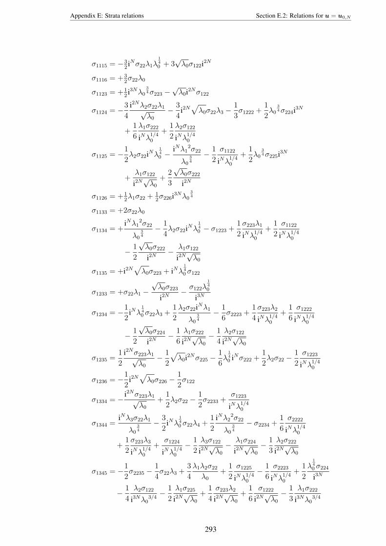
Appendix E: Strata relations Section E.2: Relations for u = u0,N
σ1115 = −32iNσ22λ1λ
140 + 3
√λ0σ122i2N
σ1116 = +32σ22λ0
σ1123 = +12i3Nλ0
34σ223 −
√λ0i2Nσ122
σ1124 = −3
4
i2Nλ2σ22λ1√λ0
− 3
4i2N√λ0σ22λ3 −
1
3σ1222 +
1
2λ0
34σ224i3N
+1
6
λ1σ222
iNλ1/40
+1
2
λ2σ122
iNλ1/40
σ1125 = −1
2λ2σ22iNλ
140 −
iNλ12σ22
λ0
34
− 1
2
σ1122
iNλ1/40
+1
2λ0
34σ225i3N
+λ1σ122
i2N√λ0
+2
3
√λ0σ222
i2N
σ1126 = +12λ1σ22 + 1
2σ226i3Nλ0
34
σ1133 = +2σ22λ0
σ1134 = +iNλ1
2σ22
λ0
34
− 1
4λ2σ22iNλ
140 − σ1223 +
1
2
σ223λ1
iNλ1/40
+1
2
σ1122
iNλ1/40
− 1
2
√λ0σ222
i2N− λ1σ122
i2N√λ0
σ1135 = +i2N√λ0σ223 + iNλ
140 σ122
σ1233 = +σ22λ1 −√λ0σ223
i2N− σ122λ
140
i3N
σ1234 = −1
2iNλ
140 σ22λ3 +
1
2
λ2σ22iNλ1
λ0
34
− 1
6σ2223 +
1
4
σ223λ2
iNλ1/40
+1
6
σ1222
iNλ1/40
− 1
2
√λ0σ224
i2N− 1
6
λ1σ222
i2N√λ0
− 1
4
λ2σ122
i2N√λ0
σ1235 =1
2
i2Nσ223λ1√λ0
− 1
2
√λ0i2Nσ225 −
1
6λ
140 iNσ222 +
1
2λ2σ22 −
1
2
σ1223
iNλ1/40
σ1236 = −1
2i2N√λ0σ226 −
1
2σ122
σ1334 = − i2Nσ223λ1√λ0
+1
2λ2σ22 −
1
2σ2233 +
σ1223
iNλ1/40
σ1344 =iNλ3σ22λ1
λ0
34
− 3
2iNλ
140 σ22λ4 +
1
2
iNλ22σ22
λ0
34
− σ2234 +1
6
σ2222
iNλ1/40
+1
2
σ223λ3
iNλ1/40
+σ1224
iNλ1/40
− 1
2
λ3σ122
i2N√λ0
− λ1σ224
i2N√λ0
− 1
3
λ2σ222
i2N√λ0
σ1345 = −1
2σ2235 −
1
4σ22λ3 +
3
4
λ1λ2σ22
λ0
+1
2
σ1225
iNλ1/40
− 1
6
σ2223
iNλ1/40
+1
2
λ140 σ224
i3N
− 1
4
λ2σ122
i3Nλ03/4− 1
2
λ1σ225
i2N√λ0
+1
4
σ223λ2
i2N√λ0
+1
6
σ1222
i2N√λ0
− 1
3
λ1σ222
i3Nλ03/4
293

Appendix E: Strata relations Section E.2: Relations for u = u0,N
σ1346 = −1
6σ222 −
1
2σ2236 −
1
4
λ2σ22
iNλ1/40
+1
2
σ1226
iNλ1/40
− 1
2
λ1σ226
i2N√λ0
σ2333 = −2λ1σ22i3N
λ1/40
− 3iNλ1/40 σ223
σ2334 =1
2σ22λ3 +
1
3
σ2223
iNλ1/40
− 1
2
σ223λ2
i2N√λ0
− λ1/40 σ224
i3N
σ2335 = −iNλ1/40 σ225 −
2
3σ222 −
1
2
σ2233
iNλ1/40
+λ2σ22
iNλ1/40
σ2336 = −iNλ1/40 σ226 − σ223
σ2344 =1
2
λ2σ22iNλ3
λ03/4
− 2iNλ1/40 σ22 +
1
2
σ223λ4
iNλ1/40
+1
3
σ2224
iNλ1/40
− 1
6
σ222λ3
i2N√λ0
− 1
2
σ224λ2
i2N√λ0
σ2345 = −1
2σ22λ4 +
3
8
λ22σ22
λ0
+1
6
σ2225
iNλ1/40
− 1
2
σ2234
iNλ1/40
+1
12
σ2222
i2N√λ0
− 1
4
σ225λ2
i2N√λ0
+1
4
σ223λ3
i2N√λ0
− 1
4
λ2σ222
i3Nλ03/4
σ2346 = −1
2σ224 +
1
6
σ2226
iNλ1/40
− 1
4
σ226λ2
i2N√λ0
σ2355 = − σ2235
iNλ1/40
+σ22λ3
iNλ1/40
− 1
3
σ2223
i2N√λ0
+1
2
σ223λ2
i3Nλ03/4
σ2356 = −1
2σ225 −
1
2
σ222
iNλ1/40
− 1
2
σ2236
iNλ1/40
+1
2
λ2σ22
i2N√λ0
σ2366 = −σ226 +1
2
σ223
iNλ1/40
σ2566 = −1
2
λ2σ22iN
λ03/4
+1
2
σ225
iNλ1/40
− 1
2
σ2266
iNλ1/40
+1
3
σ222
i2N√λ0
σ3334 = σ222 +3
2
σ2233
iNλ1/40
− 5
2
λ2σ22
iNλ1/40
σ3344 = 2σ22λ4 −λ2
2σ22
2λ0
+ 2σ2234
iNλ1/40
− σ223λ3
i2N√λ0
− 1
6
σ2222
i2N√λ0
+1
3
λ2σ222
i3Nλ03/4
σ3345 =σ2235
iNλ1/40
− σ22λ3
iNλ1/40
+1
3
σ2223
i2N√λ0
− 1
2
σ223λ2
i3Nλ03/4
σ3346 =1
3
σ222
iNλ1/40
+σ2236
iNλ1/40
σ3444 =3
4
iNσ22λ32
λ03/4
+ 3/4iNλ4λ2σ22
λ03/4
+3
2
σ223
iNλ1/40
+3
2
σ2244
iNλ1/40
− 3
2
σ224λ3
i2N√λ0
− 1
2
σ222λ4
i2N√λ0
294

Appendix E: Strata relations Section E.2: Relations for u = u0,N
σ3445 = −σ22 +3
4
λ2σ22λ3
λ0
+σ2245
iNλ1/40
− 1
2
σ225λ3
i2N√λ0
+1
3
σ2224
i2N√λ0
− 1
3
σ222λ3
i3Nλ03/4− 1
2
σ224λ2
i3Nλ03/4
σ3446 = −1
2
σ22λ4
iNλ1/40
+σ2246
iNλ1/40
− 1
2
σ226λ3
i2N√λ0
σ3455 = − σ22λ4
iNλ1/40
+1
2
σ2255
iNλ1/40
+1
2
λ22σ22
iNλ05/4
+1
3
σ2225
i2N√λ0
− 1
2
σ225λ2
i3Nλ03/4
+1
12
σ2222
i3Nλ03/4− 1
3
λ2σ222
λ0
σ3456 = −1
2
σ224
iNλ1/40
+1
2
σ2256
iNλ1/40
+1
6
σ2226
i2N√λ0
+1
4
σ22λ3
i2N√λ0
− 1
4
σ226λ2
i3Nλ03/4
295

Bibliography
[1] S. Abenda and Yu. N. Fedorov. On the weak Kowalevski-Painleve property for hy-
perelliptic seperable systems. Acta Applicandae Mathematicae, 60:138–178, 2000.
[2] M.S. Alber and Yu. N. Fedorov. Wave solutions of evolution equations and Hamilto-
nian flows on nonlinear subvarieties of generalised Jacobians. Journal of Physics A:
Mathematical and Theoretical, 33:8409–8425, 2000.
[3] J.V. Armitage and W.F. Eberlein. Elliptic functions — LMS student texts 67.
Cambridge, 2006.
[4] C. Athorne. Identities for hyperelliptic ℘-functions of genus one, two and three in
covariant form. Journal of Physics A: Mathematical & Theoretical, 41:415202, 2008.
[5] C. Athorne, J.C. Eilbeck, and V.Z. Enolskii. Identities for the classical genus two
℘-function. Journal of Geometry and Physics, 48(2-3): 354–368, 2003.
[6] C. Athorne, J.C. Eilbeck, and V.Z. Enolskii. A sl(2) covariant theory of genus 2
hyperelliptic functions. Mathematical Proceedings of the Cambridge Philosophical
Society, 136(2): 269–286, 2004.
[7] H.F. Baker. Abelian functions: Abel’s theorem and the allied theory of theta functions.
Cambridge University Press, 1897 (Reprinted in 1995).
[8] H.F. Baker. On the hyperelliptic sigma functions. American Journal of Mathematics,
20:301–384, 1898.
[9] H.F. Baker. On a system of differential equations leading to periodic functions. Acta
Mathematica, 27:135–156, 1903.
[10] H.F. Baker. Multiply periodic functions. Cambridge University Press, Cambridge,
1907 (Reprinted in 2007 by Merchant Books. ISBN 193399880).
[11] S. Baldwin, J.C. Eilbeck, J. Gibbons, and Y. Onishi. Abelian functions for cyclic
trigonal curves of genus four. Journal of Geometry and Physics, 58:450–467, 2008.
[12] S. Baldwin and J. Gibbons. Hyperelliptic reduction of the Benney moment equations.
Journal of Physics A: Mathematical and Theoretical, 36:8393, 2003.
296

Bibliography
[13] S. Baldwin and J. Gibbons. Higher genus hyperelliptic reductions of the Benney
equations. Journal of Physics A: Mathematical and Theoretical, 37:5341–5354, 2004.
[14] S. Baldwin and J. Gibbons. Genus 4 trigonal reduction of the Benny equations. Jour-
nal of Physics A: Mathematical and Theoretical, 39:3607–3639, 2006.
[15] E. Bellman. A brief introduction to theta functions. Holt, Rinehart and Winston, 1961.
[16] E.D. Belokolos, A.I. Bobenko, V.Z. Enolskii, A.R. Its, and V.B. Matveev. Algebro-
geometric approach to nonlinear integrable equations. Springer Verlag, 1994.
[17] D.J. Benney. Some properties of long nonlinear waves. Studies in Applied Mathemat-
ics, 52:45, 1973.
[18] O. Bolza. On the first and second derivatives of hyperelliptic σ-functions. Mathema-
tische Annalen, 17:11–36, 1895.
[19] V.M. Buchstaber, V.Z. Enolskii, and D.V. Leykin. Kleinian functions, hyperelliptic
Jacobians and applications. Reviews in Math. and Math. Physics, 10:1–125, 1997.
[20] V.M. Buchstaber, V.Z. Enolskii, and D.V. Leykin. Rational analogs of Abelian func-
tions. Functional Analysis and its Applications, 33:83–94, 1999.
[21] V.M. Buchstaber, V.Z. Enolskii, and D.V. Leykin. Uniformization of Jacobi varieties
of trigonal curves and nonlinear equations. Functional Analysis and its Applications,
34:159–171, 2000.
[22] V.M. Bukhshtaber, D.V. Leikin, and V.Z. Enol’skii. σ-functions of (n, s)-curves. Com-
munications of the Moscow Mathematical Society, 54:No. 3, 1999.
[23] J.L. Burchnall and T.W. Chaundy. Commutative ordinary differential operators. Pro-
ceedings of the London Mathematical Society, 118:420–440, 1923.
[24] H. Burkhardt. Beitrage zur theorie der hyperelliptische sigmafunctionen. Mathema-
tische Annalen, 32:381–442, 1888.
[25] J.W.S. Cassels and E.V. Flynn. Prolegomena to a middlebrow arithmetic of curves of
genus 2 — LMS Lecture note series 230. Cambridge, 1996.
[26] K. Chandrasekharan. Elliptic functions. Springer Verlag, 1985.
[27] H. Cohen and G. Frey. Handbook of elliptic and hyperelliptic curve cryptography.
Chapman and Hall / CRC, 2006.
[28] P. DulVal. Elliptic functions and elliptic curves — LMS Lecture note series 9. Cam-
bridge University Press, 1973.
297

Bibliography
[29] J.C. Eilbeck. http://www.ma.hw.ac.uk/Weierstrass/Trig34/.
[30] J.C. Eilbeck, V.Z. Enolski, S. Matsutani, Y. Onishi, and E. Previato. Abelian functions
for trigonal curves of genus three. International Mathematics Research Notices, page
Art.ID: rnm140 (38 pages), 2007.
[31] J.C. Eilbeck, V.Z. Enolski, S. Matsutani, Y. Onishi, and E. Previato. Addition formulae
over the Jacobian pre-image of hyperelliptic wirtinger varieties. Journal fr die reine
und angewandte Mathematik (Crelle’s Journal), 618:37–48, 2008.
[32] J.C. Eilbeck and V.Z. Enolskii. Bilinear operators and the power series for the Weier-
strass σ function. Journal of Physics A: Mathematical and Theoretical, 33:791–794,
2000.
[33] J.C. Eilbeck, V.Z. Enolskii, and E.Previato. Varieties of elliptic solitons. Journal of
Physics A: Mathematical and Theoretical, 34:2215–2227, 2001.
[34] J.C. Eilbeck, V.Z. Enolskii, and E.Previato. On a generalized Frobenius–Stickelberger
addition formula. Letters in Mathematical Physics, 65:5–17, 2003.
[35] J.C. Eilbeck, V.Z. Enolskii, and D.V. Leykin. On the Kleinian construction of Abelian
functions of canonical algebraic curves. In D Levi and O Ragnisco, editors, Proceed-
ings of the 1998 SIDE III Conference, 1998: Symmetries of Integrable Differences
Equations, volume CRMP/25 of CRM Proceedings and Lecture Notes, pages 121–
138, 2000.
[36] J.C. Eilbeck, S. Matsutani, and Y. Onishi. Some addition formula for Abelian func-
tions for elliptic and hyperelliptic curves of cyclotomic type.
preprint,arXiv:0803.3899v1, 2008.
[37] M. England. http://www.ma.hw.ac.uk/∼matte/BenneyReduction/.
[38] M. England. http://www.ma.hw.ac.uk/Weierstrass/45Results/.
[39] M. England and J.C. Eilbeck. Abelian functions associated with a cyclic tetragonal
curve of genus six. Journal of Physics A: Mathematical and Theoretical, 42:095210
(27pp), 2009.
[40] M. England and J. Gibbons. A genus six cyclic tetragonal reduction of the Benney
equations. Journal of Physics A: Mathematical and Theoretical, 42:375202 (27pp),
2009.
[41] V.Z. Enolskii, M. Pronine, and P.H. Richter. Double pendulum and θ-divisor. Journal
of Nonlinear Science, 13:157–174, 2003.
[42] H.M. Farkas and I. Kra. Riemann surfaces — Second edition. Springer, 1992.
298

Bibliography
[43] I.M. Gelfand, M.M. Kapranov, and A.V. Zelevinsky. Discriminants, resultants and
multidimensional determinants. Birkhauser, 1994.
[44] J. Gibbons. Collisionless boltzmann equations and integrable moment equations.
Physica D, 3:503, 1981.
[45] G. Goppel. Theoriae transcendentium Abelianarum primi ordinis adumbrato levis.
Journ.reine angew. Math, 35:277, 1847.
[46] P. Griffiths and J. Harris. Principles Of Algebraic Geometry. Wiley-Interscience,
1978.
[47] E. Hackmann and C. Lammerzahl. Complete analytic solution of the geodesic
equation in Schwarzschild-(Anti-)de Sitter spacetimes. Physical Review Letters,
100:171101, 2008.
[48] S.P. Tsarev J. Gibbons. Reductions of the Benney equations. Physics Letters A,
211:19, 1996.
[49] S.P. Tsarev J. Gibbons. Conformal maps and reductions of the Benney equations.
Physics Letters A, 258, 1999.
[50] J. Jorgenson. On directional derivatives of the theta function along its divisor. Israel
Journal of Mathematics, 77:273–284, 1992.
[51] F. Klein. Uber hyperelliptische sigmafunctionen. Mathematische Annalen, 32:351–
380, 1888.
[52] B.A. Kupershmidt and Yu.I. Manin. Long-wave equation with free boundaries. Func-
tional Analysis and its Applications, 11:188, 1977.
[53] S. Lang. Introduction to algebraic functions and Abelian functions. Number 89 in
Graduate Texts in Mathematics. Springer-Verlag, 2nd. edition, 1982.
[54] D. Lawden. Elliptic Functions and Applications. Springer Verlag, 1980.
[55] H. Ludmark. Complex analysis: Elliptic functions
http://www.mai.liu.se/ halun/complex/elliptic/.
[56] I.G. Macdonald. Symmetric Functions and Hall polynomials. Clarendon Press, Ox-
ford, 1995.
[57] H. McKean and V. Moll. Elliptic curves. Cambridge, 1997.
[58] R. Miranda. Algebraic curves and Riemann surfaces. AMS, 1995.
299

Bibliography
[59] D. Mumford. Tata lectures on Theta I, volume 28 of Progress in Mathematics.
Birkhauser, Boston, 1983.
[60] A. Nakayashiki. On algebraic expressions of sigma functions for (n, s)-curves.
preprint, arXiv:0803.2083v1, 2008.
[61] Proceedings of symposia in pure mathematics. Theta functions: Bowdoin: Volume
49, Part 1 & 2. AMS, 1987.
[62] Y. Onishi. Determinant expressions for hyperelliptic functions. Proceedings of the Ed-
inburgh Mathematical Society, 48(3):705–742, 2005. (With an appendix by Shigeki
Matsutani).
[63] Y. Onishi. Abelian functions for trigonal curves of degree four and determinantal
formulae in purely trigonal case. International Journal of Mathematics, 20(4):427–
441, 2009.
[64] G. Rosenhain. Abhandlung uber die functionen zweier variabler mit vier perioden.
Mem. pre l’Acad de Sci. de France des savants, IX:361–455, 1851.
[65] W. Schreiner, C. Mittermaier, and K. Bosa. Distributed Maple: Parallel computer
algebra in networked environments. Journal of Symbolic Computation, 35:305–347,
2003.
[66] S.P. Tsarev. The geometry of Hamiltonian systems of hydrodynamic type. The gener-
alized hodograph method. Izvestiya: Mathematics, 37:397, 1991.
[67] L.C. Washington. Elliptic curves: Number theory and cryptography. Chapman and
Hall / CRC, 2003.
[68] K. Weierstrass. Beitrag zur theorie der Abel’schen integrale. Jahreber, Konigl. Ka-
tolischen Gymnasium zu Braunsberg in dem Schuljahre, pages 3–23, 1848/1849.
[69] K. Weierstrass. Zur theorie der Abelschen functionen. Journ.reine angew. Math,
47:289–306, 1854.
[70] E.T. Whittaker and G.N. Watson. A course of modern analysis. Cambridge, 1947.
[71] E. Wiltheiss. Ueber die potenzreihen der hyperelliptischen thetafunctionen. Mem. pre
l’Acad de Sci. de France des savants, 31:410–423, 1888.
[72] W.Schreiner. www.risc.uni-linz.ac.at/software/distmaple/.
[73] L. Yu and J. Gibbons. The initial value problem for reductions of the Benney equa-
tions. Inverse Problems, 16:605–618, 2000.
[74] V.E. Zakharov. On the Benney equations. Physica D, 3:193, 1981.
300


![Unified approach to Miura, B¨acklund and Darboux ... · Geometry and Abelian Function theory [34]. Jacobi elliptic functions have associated with them a genus 2 Riemann surface](https://static.fdocuments.us/doc/165x107/5f701f64abe8397dc027281e/uniied-approach-to-miura-backlund-and-darboux-geometry-and-abelian-function.jpg)