High Unemployment Yet Few Small Firms: The Roleof Centralized Bargaining in South Africa

Jeremy R. Magruder∗

November 11, 2011

Abstract

South Africa has very high unemployment, yet few adults work informally in smallfirms. This paper tests whether centralized bargaining, by which unionized largefirms extend arbitration agreements to non-unionized smaller firms, contributes to thisproblem. While local labor market characteristics influence the location of theseagreements, their coverage is spatially discontinuous, allowing identification by spatialregression discontinuity. Centralized bargaining agreements are found to decrease em-ployment in an industry by 8-13%, with losses concentrated among small firms. Theseeffects are not explained by resettlement to uncovered areas, and are robust to a widevariety of controls for unobserved heterogeneity.

∗University of California, Berkeley. I thank Guojun He and Charles Seguin for excellent research as-sistance and John Bellows for alerting me to some of the data used in this study. I also thank MichaelAnderson, Lori Beaman, Tim Conley, Ann Harrison, Elisabeth Sadoulet, Paul Schultz, Chris Udry andseminar audiences at Berkeley, USC, UCSD, the World Bank, the University of Stellenbosch, the Universityof Cape Town, The University of the Witwatersrand, the University of Pretoria, Yale, and Northwesternfor many helpful comments, and also Economic Research Southern Africa for organizing a workshop andfacilitating seminars in South Africa. All remaining mistakes are naturally my own.

1

1 Introduction

Wage-setting institutions, including collective bargaining and labor legislation, are politically

charged issues for countries at all stages of development. Concern over the first-order

theoretical implications of these labor market distortions —that mandating improved working

conditions should induce lower employment —has been somewhat attenuated by the vast

empirical literature which has examined these issues. The large majority of these studies

have taken place in OECD countries, and are characterized by a finding of small employment

effects (Blau and Kahn 1999; for a survey of evidence from developing countries see Freeman

2009). It seems likely that the labor market response to wage-setting institutions changes as

countries develop. After all, for wage-employment tradeoffs to be economically important,

two structural features must hold: first, there must be substantial labor supply at low wages

(below the cut of the proposed standards), and second, the government must have the

capacity to actually enforce these regulations. We might expect labor markets in middle

income countries to exhibit these two features, and particularly so in countries with high

rates of inequality. There, a large fraction of the labor force experiences living standards

similar to those in much poorer countries and may be willing to work at very low wages.

At the same time, the government’s tax base and enforcement capacity may have grown

stronger, attaching credibility to labor law1.

In South Africa, a middle income country with very high inequality, the labor market

appears heavily distorted. Similar to many other low and middle income countries, for-

mal sector work is dominated by large scale employers, where it is highly regulated, highly

remunerated, and scarce. However, very differently than many peer countries, there are

few small firm jobs of any sort, informal or otherwise2. The outcome is an astronomical

1Indeed, previous studies of minimum wages in Latin America have provided evidence that minimumwage increases yield increases in wages in both the formal and informal sectors (Freeman 2009), suggestingthat legislated labor standards can impact the labor market across the labor supply distribution in middleincome countries.

2For an extended discussion of small firms in developing countries, see Liedholm and Mead (1987, 1999).

2

unemployment rate, where only 56% of prime-aged men and 40% of prime-aged women are

actually working. Understanding why there is so little employment in small firms is a ques-

tion of fundamental policy importance to South Africa. This is particularly true if labor

standards contribute to the problem, as then policy prescriptions are immediate. In that

case, conclusions may also have direct analogues when similar policies are implemented in

other contexts.

While there are many labor regulations in South Africa, one particular form of labor

standards which has been implicated in the lack of small firms is the bargaining council

system3. Similar to centralized bargaining structures across Western Europe (Nickell 1997)

and in Argentina and Brazil (Carneiro 1997; Cardoso and Gindin 2009), employer organi-

zations and unions may opt to participate in bargaining councils, which extend arbitration

agreements beyond the firms and unions which make them to all workers in an industry in a

given political demarcation, regardless of firm size or participation in the arbitration process.

If large firms and unions agree to high standards with the goal of reducing competition from

small firms, then this could limit the viability of small firm enterprise, restricting the options

available to the unemployed. However, despite the importance of centralized bargaining

in a variety of countries, there have been few empirical studies which have provided strong

causal evidence of the employment or industrial structure effects of centralized bargaining

agreements in any context, leaving us with scant evidence to inform policy.

Understandably, then, these bargaining councils are at the center of a vigorous policy

debate in South Africa, with small firms arguing that the labor standards impose unfair costs,

while large firms assert that these labor standards are not punitive and union alliances argue

that they are necessary for worker protection. However, clean identification of the effects

of these agreements on employment and industrial structure which could inform policy has

been elusive thus far. There are several challenges to identification. First, other potential

3Presumably, informal firms could not be compelled to comply with bargaining council agreements andthus the presence of this or any other labor law seems unlikely to be the primary reason for the absence ofinformal small firms.

3

motivations for South Africa’s unemployment without entrepreneurship abound, many of

which are surely empirically relevant. For example, high wages and an extensive social

safety net may increase the demand for leisure or render long periods of unemployed search

more palatable. Entrepreneurial opportunities may be limited by low skill levels, liquidity

constraints, and high crime, while high capital stocks may make large firms competitive with

relatively low labor inputs. Moreover, the legacy of Apartheid looms large; the majority

black population was prohibited from entrepreneurship during Apartheid. While these laws

are no longer in place, their effects on skillsets and culture may have a lingering impact.

Identifying the employment effects of labor regulations, therefore, requires a careful analysis

which would hold these conditions constant. Further complicating analysis, these agreements

are outcomes of a complex bargaining process between unions and firms with unclear and

likely anti-competitive motives. Since centralized bargaining is not mandated, the firms

which choose to pursue centralized bargaining may be those who work in local labor markets

where centralized bargaining would represent a particularly large competitive advantage.

This paper estimates the effects of bargaining councils using several methods, taking

advantage of the tremendous amount of variation in the data: agreements vary with space,

across industries, and over time. As a benchmark, a difference-in-differences estimates sig-

nificant negative effects of bargaining councils on employment and small firm employment.

As it is possible that trends in local labor market characteristics are related to secular trends

in bargaining council status, confounding that estimator, the paper then takes advantage of

the fact that local labor markets should be spatially continuous within South Africa, while

these agreements are enforced in a spatially discontinuous way. This suggests a spatial

regression discontinuity estimation. Using distance to policy regime borders as the running

variable, the spatial regression discontinuity reveals even larger negative employment effects

which are both visibly and statistically significant. Finally, this paper adopts the spatial

fixed effects proposed in Conley and Udry (2008) and Goldstein and Udry (2008) as its pre-

ferred estimator, arguing that these spatial fixed effects have several advantages over a more

4

traditional regression discontinuity in a spatial context. These spatial fixed effects estimates

report consistent and large effects: industries which have an agreement in a particular mag-

isterial district in a given year have about 8-13% lower employment and 10-21% higher wages

than the same industry in uncovered neighboring magisterial districts. Firm sizes are also

impacted, with 7-16% fewer employees in small firms and 7-15% fewer entrepreneurs, while

there are smaller and insignificant effects on large firms and single employee firms. Utiliz-

ing magisterial district-year and magisterial district-industry fixed effects, I show that these

spatial discontinuities are similar in magnitude and precision whether only inter-industry

variation (within a magisterial district-year) or intertemporal variation (within a magisterial

district-industry) is utilized, and that estimates increase in magnitude and precision if we

consider only small magisterial districts who should be unable to endogenously influence

these agreements. I further illustrate that, while firms do move across borders in order to

avoid these agreements, this border-jumping does not drive the employment effects measured

here, so that these reductions in employment represent a net loss for the economy. The ten

percent employment effect on covered industries is large relative to those which have been

identified in other labor regulation studies, and accounts for about a percentage point of

unemployment. These bargaining councils thus have an effect which is economically signif-

icant and should be of interest to policy makers both in South Africa and in other middle

income countries. However, they cannot explain the majority of unemployment in South

Africa, and therefore bargaining councils are best understood as exacerbating an existing

and severe problem.

2 South Africa’s Missing Small Firms

Unemployment in South Africa is extremely high, particularly among non-whites. The

first two columns of Table 1 report data from the 2003 Labour Force Survey (described

below), which indicates that only about 56% of 20-60 year old men and 40% of 20-60 year

5

old women are actually working (the corresponding employment rates are 50% and 35% if

we restrict our attention to the majority black population). These numbers correspond to a

34% unemployment rate in this prime-aged population (where unemployment is defined as

wanting work)4. A large number of potential reasons for this unemployment exist, and the

unemployment numbers and potential contributors for them are surveyed more extensively in

a series of papers by Kingdon and Knight (2004, 2006, 2008) as well as Banerjee et al (2008).

Wages are high, due to high capital/labor ratios, a strong union presence, and extensive

governmental labor market regulation in addition to the industrial bargaining agreements

which are the focus of this paper (e.g. Butcher and Rouse 2000, Schultz and Mwabu 1998).

Second, entrepreneurial skills may be absent in the population, as informal employment was

squashed under Apartheid (e.g. Kingdon and Knight 2004). Third, some unemployment

may be voluntary; a generous non-contributory pension program combined with the high

wages earned by the employed leave many unemployed individuals with networks capable

of supporting them (see Bertrand, Mullainathan, and Miller 2003 for labor supply effects;

Edmonds, Mammen, andMiller 2005 for network effects of pensions on living arrangements).

While it is clear that many adults are unemployed in South Africa, it is unclear what

adults are in fact doing. Labor force surveys in South Africa go to great lengths to measure

any economic activity, identifying as workers individuals who engage in unpaid household

work or tend household plots "even for only one hour" in the past week; this approach yields

the low employment numbers described above. A very natural response to this unemploy-

ment would be for many to create entreneurial work5. Yet row 2 of table 1 reveals that

only 6-8 percent of prime age South Africans are self-employed6. These numbers are tiny

compared to countries with similar levels of unemployment (e.g. Charmes 2000, Kingdon

4Kingdon and Knight (2006) advocate this broad unemployment measure in this context, as local wagesare more sensitive to that measure. Offi cial unemployment numbers include a broader range of ages andheld steady at 42% over the period of 2002-2004.

5This is particularly true as unemployment durations are very long, and there is some evidence thatsocial connections may be important to find employment. Since jobs are scarce, job opportunities may beshared among very close relations (Magruder 2010, Seekings and Nattrass 2005), leaving individuals withpoor social connections with very limited opportunities to find work.

6Among the majority black population, the corresponding figure is about 6% for both men and women

6

and Knight 2004). Moreover, what is perhaps most striking is that there are relatively few

employees of small firms in general. The remaining rows of table 1 reports the percent of

employees in each firm size category in South Africa. Particularly for men, we see very few

workers in firms of fewer than 5 employees. For comparison purposes, I also include similar

data from the 1995-96 Brazillian LSMS survey7. We see that, while unemployment is a

great deal higher in South Africa, the distribution of firm sizes looks fairly similar —with

one big exception. What is missing in South Africa, compared to Brazil, are the small firms

with 2-4 employees.

Of the above explanations for high unemployment, one in particular which may suggest

minimal small-scale employment in a high unemployment context is well-enforced labor regu-

lation. The South African labor market is highly regulated, with a variety of legislated labor

standards as well as privately bargained arbitration decisions. Unlike many other developing

countries, South Africa is successful in enforcing labor and tax regulations on many small

firms; an influential study found that the average business with fewer than 5 employees pays

nearly R14000 (about $2170) per employee in costs associated with tax and labor regula-

tions8(SBP 2005). Moreover, unions and firms can extend labor standard arbitration to all

workers in a given political district through bargaining councils. Small businesses, in par-

ticular, have advocated aggressively against the extension of these labor standards; in 2005

South African President Thabo Mbeki announced that small businesses would be granted a

blanket exemption from these bargaining council agreements within the year in his state of

the union address (Mbeki 2005). However, under pressure from trade unions and employers

organizations to the contrary, the government never enacted this blanket exemption (e.g.

Cosatu Rejects 2005). The fact both that the government would consider a legal change to

7It is not common for household surveys in developing countries to ask respondents about the size of thefirm they work for. Fortunately, the Brazillian LSMS is an exception. Brazil represents a particularly goodcomparison for South Africa as a country with a broadly similar income level and similarly extreme level ofinequality.

8This estimate is the average over complying and non-complying firms. The greatest contributor to thisestimated cost is VAT, though labor regulations are also important. Of course, small business respondentsto this survey may overstate compliance.

7

exempt small business and that it meant with strong opposition confirms the anecdotal and

survey evidence that these regulations are enforceable.

The potential of labor regulations to affect employment has been extensively explored

in economics and found generally mixed results; surveys of this literature are available in

Blau and Kahn (1999), Freeman (2009), and Nickell and Layard (1999). Much of the recent

literature (e.g. Bertrand and Kramarz 2002, Besley and Burgess 2004, Harrison and Scorce

2008) has adopted a difference-in-differences approach where a time series of data on the

legislative environment in states is summarized by a before and after period. Difference in

employment trends between "treatment" states which adopt a policy and "control" states

which do not are then compared to estimate the effect of regulations on employment. A

second approach is to utilize a spatial discontinuity (e.g. Holmes 1998; Dube, Lester, and

Reich 2010), where neighboring counties or states are compared, under the assumption that

geographically proximate counties share similar labor markets and incentives to form labor

policy, but are differentially exposed. Many existent labor regulation studies adopt some

elements of each of these approaches (e.g. Card and Krueger 1994), so that changes in trends

are compared across spatially proximate regions. The measure of each of these studies is

how comparable of a control group can be developed without causing small sample problems;

to determine which approach is best for South Africa will require a more careful description

of the labor regulations to be studied.

3 Industrial Bargaining in South Africa

Unions in South Africa can bargain with employers in two primary ways. The 1995 La-

bor Relations Act codifies the right of employers to form employers organizations for their

particular industry and region and bargain with unions centrally; the labor standards which

result from this bargaining can then be applied to all employees working in the industry and

region which the bargaining council presides over. That is, if employer organizations and

8

unions decide to bargain centrally, then all employees who work within that geographical

region will work under the agreed-upon labor standards, regardless of their union status.

Unions and employers may also choose to bargain unilaterally, resulting in plant level agree-

ments (Bendix 2001). Both unilateral bargaining and centralized bargaining are observed

in a wide variety of industries and areas in South Africa, so that different industries in the

same location may be covered by different types of agreements, industries may be covered by

unilateral agreements in some locations and centralized agreements in others, and industries

in a particular location may be covered by centralized agreements in one year and not in

another.

It is encoded in law that bargaining councils must be representative of firms and employee

unions in their jurisdiction; however, the extent to which this law is enforced is unclear. The

offi cial wording is that councils must be "suffi ciently" representative, leading to a great deal

of bureaucratic discretion and contention (primarily from small employers) as to whether

the agreements represent all interests (Bendix 2001). South Africa’s political structure is

that 354 magisterial districts are organized into one of 52 district councils; these in turn

comprise 9 provinces. In principle, there is not a strict criteria over which groupings of

magisterial districts can form a bargaining council; in practice, most bargaining councils

represent collections of magisterial districts which map to political boundaries, either na-

tional, provincial, or at the district council level. In the model outlined below, I follow the

empirical trend in presuming that other magisterial districts within the district council are

the natural bargaining partners in determining whether to form a bargaining council agree-

ment, while empirical analysis will standardize bargaining council units to eliminate any

potential endogeneity stemming from the choice of bargaining council size (and to determine

the "potential" bargaining council units for magisterial district-industry observations which

are not covered by a bargaining council).

Existing studies on the effects of arbitration on wages and unemployment in South

Africa have imperfect information on the presence of bargaining council agreements and

9

treat the endogeneity of union membership via industry and occupational fixed effects, which

may be an imperfect control; these studies find that unions receive very high wage premia,

particularly at the bottom of the income distribution (Schultz and Mwabu 1998), and that

bargaining councils exhibit a smaller, though still present, wage premium (Butcher and

Rouse 2001). However, since the right to bargain centrally is one which must be exercised

voluntarily, we may be concerned that bargaining council agreements exist systematically

in the industries, magisterial districts, and years in which local labor markets make them

particularly profitable for the firms who pursue centralized bargaining.

Moll (1996) outlines a theoretical model discussing the implications of bargaining councils

for large and small firms. We may also imagine that large firm incentives depend on whether

the large firm is unionized. Suppose that, in the absence of a bargaining council agreement,

large unionized firms pay privately bargained wages(wU), while large non-unionized firms

and small firms pay market wages (w∗). Under a bargaining council agreement, all would

pay the same bargaining council wage(wBC

); following Moll (1996) in presuming that wU >

wBC > w∗, it is clear that operating costs decrease for large unionized firms and increase for

small firms and large non-unionized firms in the presence of a bargaining council agreement.

As the supply curves for the three types of firms shift, equilibrium changes. If small firms

have the lowest marginal products of labor (due to low capital stocks), we may imagine that

their supply curve shifts in by the largest margin, resulting in an increase in the residual

demand faced by the two types of large firms. Thus, large unionized firms benefit from

less competition from small firms and lower wages, large non-unionized firms benefit from

less competition from small firms but suffer from higher wages, and small firms lose by the

greatest margins. The degree of these benefits, and the degree to which small firms and large

non-unionized firms are punished by the bargaining council agreement, are functions of local

demand, local labor supply, production technologies at each firm size, and other local labor

market characteristics, as the changes in the demand faced by each type of firm will depend

on anything which influences local supply and demand curves. While the intuition behind

10

these labor market responses is straightforward, I develop a model in the web appendix which

shows more formally that large unionized firms will increase employment in response to a

bargaining council agreement, while large non-unionized firms and small firms will decrease

employment.

The differing profit incentives that employers face, outlined above, are clear. Therefore,

the presence of a bargaining council agreement will clearly be related to some aggregation of

the private incentives of the large firms who initiate centralized bargaining. However, unions

could adopt a bargaining position which is more or less hostile to bargaining councils, so the

decision to pursue centralized bargaining may depend on both firm and union incentives.

Since most of South Africa’s unions are aggregated into three large nationwide alliances

who have centralized general policies towards bargaining councils (Bendix 2001), I model

the union’s role in bargaining as a cost C of adopting the bargaining council agreement;

empirical analysis will be robust to any heterogeneity in this cost that is due to industry-

specific local labor markets or magisterial district characteristics9.

Suppose that, in the absence of a bargaining council agreement, large unionized firms in

magisterial district m earn profits πUm, and that large non-unionized firms earn π∗m. Further

suppose that all large firms each earn profits πBCm in the presence of a bargaining council

agreement before paying cost C to the union, and that fraction λm of the total Qm large firms

in magisterial district m are unionized. A bargaining council agreement is a collective result

of the preferences of large firms throughout a district council, thus, if magisterial district m

belongs to district council DC, bargaining council legislation is adopted if

∑m∈DC

QmπBCm − C >

∑m∈DC

Qm(λmπ

Um + (1− λm) π∗m

)(1)

9Both COSATU’s (South Africa’s largest union alliance) offi cial positions on bargaining council agree-ments and the discussion of commentators (e.g. Bendix 2001) suggest that unions have some support forthese agreements due to the greater political support they receive from advocating for globally higher laborstandards. We may also imagine that unions have varying incentives related to local labor market hetero-geneity, for example, the amount of dues which can be received or local competition from uncovered workers.Empirical analysis will be robust to both of these possibilities.

11

Local labor demand, local labor supply, local production technologies, local unionization

rates, and local product demand all determine the result of this relationship. In places

where small firm production technologies are relatively ineffi cient, and large firms face little

competition, the incentives to form a bargaining council agreement are weakened, while in

places with a vibrant small firms sector, the incentives to enforce uniform wages may be

high. Any econometric investigation into the effect of bargaining councils on employment

and small firm employment would have to take these local labor market characteristics into

account.

4 Data and Descriptives

Data are drawn primarily from two sources. The South African Labour Force Surveys are

a nationally representative rotating panel conducted twice yearly from 2000 through the

present, each iteration surveying around 70,000 people. I use the September surveys from

2000-2003. Unfortunately, the panel aspect has not been well-maintained, with household

identifiers not remaining consistent from wave to wave. As such, I aggregate data to the

magisterial district level and use it as a panel at that level. These data are not intended to

be representative at the magisterial district level and are not publicly released at that level

to prevent mistaken inference (on, for example, the extent of the variation in employment in

a particular magisterial district year to year). This concern, however, should not limit more

robust econometric analysis, so long as the degree to which the data are not representative is

unrelated to the variables of interest and local-level unobservable heterogeneity is properly

controlled for. While magisterial district identifiers are not released, they can be inferred

from personal identification codes. These identifiers remain unchanged since at least the

1997 October Household Survey, which published an association between number and local

municipality names10. From this list, I determine the magisterial district of each sampling

10Examining characteristics of magisterial districts between these two surveys reassures that the identifiersare in fact unchanged. A change in coding in 2004 limits the sample to 2000-2003.

12

area, and determine the longitude and latitude for the population center of that magisterial

district. The unit of analysis in this paper will thus be the magisterial district; since

sampling weights are not designed to be representative at this level I do not use them.

Therefore, I measure employment in a given industry in a given magisterial district as the

number of people surveyed in that magisterial district who work in that industry11. We

may be concerned that very large magisterial districts have different labor markets from

their neighbors, and that we get little useful information out of small magisterial districts

where relatively few individuals were surveyed. I exclude the top and bottom two percent

of magisterial districts in terms of population from the analysis. Summary statistics of the

variables which will be used are included in table 2.

The presence of bargaining council agreements in a given year is revealed by the South

African Government Gazette, which publishes all agreements. A database compiled by the

author reveals which industries in which magisterial districts were covered by an agreement in

each year. This yields the outcome that 15 two-digit industries in South Africa are covered by

bargaining council agreements for at least some of the sample period. Of these, 7 industries

have cross-sectional variation in their coverage across the district councils of South Africa.

In 2003, 22% of prime-age African and Coloured workers in South Africa work in two-digit

industries where, in their magisterial district, some workers are covered by a bargaining

council agreement12. Different industries have different minimum effective scales, limiting

the potential for entrepreneurship in some industries. Table 3 reveals that 75% of the prime-

age African and Coloured self-employed in South Africa work in two-digit industries which at

11In a related point, it is not immediately obvious how to treat observations of 0 employment in somecategory in a particular town (of which there are many). On the one hand, these observations give usefuland important variation — if bargaining councils are brutally effective, we may expect to see 0 small firmemployees in a particular town-industry. On the other hand, when I (ultimately) take log+1 as a measureof employment, the log operator strongly emphasizes observations which are 0. This concern is lessened bythe use of the simple count data rather than weighted counts —the difference between log(1) and log(301) isa lot more than the difference between log(1) and log(2). Results which use the fraction of the populationemployed in that industry (available from the author) are similar in sign and in general more preciselyestimated than the logged results presented here.12The actual number of covered workers is probably lower, due to the aggregation at the 2 digit level.

Aggregation challenges are addressed below.

13

least sometimes have bargaining councils —this suggests that these councils are being utilized

more in industries where small scale firms are economically viable. In contrast, only about

43% of workers overall are working in these industries. Looking within industries which at

least sometimes have a bargaining council, we see an even more interesting result. 48% of

employees who work in one of these industries are covered by a bargaining council agreement.

However, only 34% of self employed and 37% of small firm employees are covered, in contrast

with 69% of large firm employees — that is, among industries which at least sometimes

have bargaining council agreements, places with bargaining council agreements have limited

small scale and self employment. The industries and the percentage of employment-weighted

magisterial districts covered in years 2000 and 2003 are listed in table 4. These bargaining

councils cover heterogeneous places in South Africa, and there is substantial variation, both

geographical and intertemporal. In the appendix, I present maps showing which magisterial

districts I code as always, sometimes, or never covered by a bargaining council agreement in

each industry, as well as a table which identifies the number of magisterial districts which

add and remove bargaining councils in each industry in each year. Industries are quite

heterogeneous in their coverage patterns.

Industries are aggregated to the two-digit level. While many of the bargaining councils

are defined over two-digit industries, some are defined in a different way than the standard-

ized coding used in the labour force survey, and so only include subsets of those two-digit

industries (subsets which unfortunately do not always map to three-digit industries, the unit

reported in the surveys). This means that my measure of coverage includes individuals who

are actually working in distinct, uncovered jobs as well as covered employees. In principle,

this bias seems likely to result in conservative estimates due to measurement error, since the

bargaining council agreements only cover a fraction of the workers in the two-digit indus-

try. Two of the industries with variation end up in "other" categories. We might worry

that these categories are more heterogeneous than other two-digit designations, and that

the bargaining councils represented (hairdressing, laundry services, and contract cleaning)

14

represent a smaller fraction of the workers in the "other services" and "other business ac-

tivities" industries. Additionally, a third industry (electrical manufacturing) is very small

in scale (with only 25 small firm employees measured in South Africa across the 4 survey

years considered here), and covered almost everywhere. I exclude these three industries in

the analysis below, although similar analysis including these industries is available from the

author.

5 Econometric Model

The focus of this paper will be on estimating bargaining council effects on employment, firm

size, and wages. Model predictions suggested that bargaining councils may reduce overall

employment and small firm employment, but that they should have an ambiguous effect on

large firm employment. A linearized structural equation is given by

Yimt = α + β1BCimt + ΓXimt + ξi + δt + νimt (2)

where Yimt may be employment, employment by firm size, or wages in industry i in

magisterial district m during year t; BCimt denotes the presence of a bargaining council

agreement, and Ximt are covariates including population and, in different specifications,

magisterial district, magisterial district-year, or magisterial district-industry fixed effects.

The discussion above suggests that the presence of a bargaining council agreement is related

to many characteristics of local labor markets, including labor supply, small firm production

technologies, etc. These are contained in νimt, which may be correlated with BCimt and

other explanatory variables. Below, I’ll consider several assumptions on νimt to generate

a variety of potential control groups and illustrate the robustness of identified trends to a

variety of underlying assumptions.

Presuming we can adequately characterize νimt and develop a comparable control group,

any analysis still requires a standardization on bargaining council size. As discussed above,

15

bargaining council agreements usually apply to all magisterial districts which belong to a

larger political entity, either a district council, province, or the entire nation. However,

in a few cases individual magisterial districts are added or subtracted from these groups in

the coverage of a bargaining council (usually either the biggest magisterial district or closest

neighbors of an adjoining district council). In fact, in a few cases bargaining councils cover

only a single magisterial district. Though these observations represent a small share of the

data, we may still worry about the implications of these observations for analysis, particu-

larly in the estimates which emphasize differences across space at bargaining council borders

and which are the focus of this paper. Moreover, this fact forces consideration of poten-

tial bargaining council sizes for places with no current bargaining council in constructing

adequate control groups, which is necessary to identify the proper unit of analysis.

A direct solution to this problem is to treat bargaining council adoption as incomplete

take-up as discussed in the impact evaluation literature. In that literature, presuming we

have exogenous assignment of treatment but incomplete take-up among the treated, the

common solution is to instrument actual treatment status with assignment to treatment. I

follow that approach in this paper. Since most bargaining councils are assigned at larger

political boundaries than magisterial districts, I describe a magisterial district-industry-year

observation as eligible for the program if it belongs to a district council where at least

one magisterial district has a bargaining council agreement in that industry-year and use

that measure of eligibility as an instrument for program receipt. All first stages are strong:

all t-statistics of bargaining council eligibility on bargaining council status are over 9.813. A

visual first stage is presented in the appendix, which includes maps depicting both the actual

coverage and the instrumented coverage in each industry. The appendix also presents the

formal estimates of this first stage in the paper’s main specifications.

Second, regardless of the strategy used to solve the identification problem, two potential

sources of dependence among observations are well-known and relevant to this context. A

13Coeffi cients of bargaining council status on bargaining council eligibility range from 0.77 to 1.00.

16

first challenge to evaluating programs which are implemented at aggregate levels is that

if individuals in a political district have correlated error terms, or there is autocorrelation

in the error, then OLS produces inconsistent standard errors (Bertrand et al 2004). The

standard solution is to cluster at the policy group level. Since bargaining councils vary on the

district council-industry level14 (there are 208 district council-industry groups and 52 district

councils in the estimation sample), this context avoids the small group number concerns

which have challenged some past studies of governmental policies (discussed in Donald and

Lang 2007). Secondly, the error term may be spatially autocorrelated (Conley 1999). As the

primary identification strategy will rest on the difference between magisterial districts which

are physically proximate and those which are in the same political district, it is desirable

to construct standard errors which are robust to correlation amongst both groups. This

paper allows observations to be related if either they are close spatially or in either the

same district council in the primary analysis15. This is the more computationally intensive

procedure outlined in Cameron, Gelbach, and Miller (2006), and also a special case of the

Conley (1999) spatial errors if "economic distance" is defined as equal amongst individuals

who live either within a given physical distance or in the same District Council.

5.1 Econometric Benchmark 1: Difference-in-Differences

Our ability to estimate equation 2 depends on how we can characterize νimt. Differences-

in-differences remain the dominant approach in the literature and make the assumption

that E [νimt|Ximt, ξi, δy] = ν̃iDC , allowing a simple District Council-Industry fixed effect to

14Several of the bargaining councils extend agreements to entire provinces, while others operate only onthe District Council level (and a small fraction operate for even smaller units). This makes it diffi cultto know, for certain, how to categorize observations (particularly for industries and towns which are notcovered by a bargaining council agreement). The results presented here presume that, since some DistrictCouncils unilaterally receive bargaining councils, this is the true observation level (implicitly, this assumesthat bargaining councils which exist react to considerations at the District Council level). An alternateassumption would be to assume that the observation unit is the province-industry level. Results whichmake this assumption and cluster simultaneously at the spatial-industry, province-industry, and town levelare similar and available from the author.15The less robust Spatial RD analysis clusters over space and within district council-industries as I describe

below.

17

eliminate the endogeneity concern. In that case, we can estimate

Yimt = α + βBCimt + ΓXimt + ξi + δt + ν̃iDC + εimt (3)

where ξi, δt, and ν̃iDC represent industry, year, and District Council-Industry fixed ef-

fects, and Ximt includes a quartic in log population. Yimt variables include employment,

large firm employment, self employment, and small firm employment (small firms are defined

to be firms with fewer than 10 employees while large firms have more than 20), measured

as the log of that variable plus 1. Bargaining council status is instrumented with bar-

gaining council eligibility, as described in section 4.1. Panel A of table 5 performs the

difference-in-differences estimation on the main sample. All cells report the coeffi cient on

bargaining council presence for a given sample and dependent variable. Across the board, a

difference-in-differences suggests that effects of bargaining councils are negative and signifi-

cant. As bargaining council agreements come into place, employment decreases by 7%, as

does small firm and self employment. However, we may be concerned that bargaining council

agreements are being adopted or eliminated endogenously in places with specific time trends

in employment or small firm employment, thus violating the necessary assumption for a

difference-in-differences estimation.

5.2 Econometric Benchmark 2: Spatial Regression Discontinuity

An alternate assumption notes that the endogenous characteristics of local labor markets

within a given industry are likely to be spatially continuous16, so long as migration and

trade are locally feasible. Formally, let R (m) denote the set of all magisterial districts

16It is possible that, as a legacy of Apartheid, some labor market characteristics may not be spatiallycontinuous due to poor infractrusctural connections (the Apartheid government did purposefully separateracial groups). If true, this would challenge identification in this paper. I address this issue in the section6.1 by running specifications featuring either town-year or town-industry fixed effects. Since barriers whichhave lingered since Apartheid should both effect all industries in a given town and all years within the sameindustry, these approaches will be robust to this concern. As it turns out, both yield consistent results,suggesting that lingering spatial barriers do not drive the empirical trends documented here.

18

within radius R of magisterial district m, Zimt be the vector [Ximt, BCimt, ξi, δt] and ZiR(m)t

and nνiR(m)t denote the vectors of Zim′t and νim′t, ∀m′ ∈ R (m) . Then, spatial continuity

suggests that

E[νimt|ZiR(m)t

]= E

[νim′t|ZiR(m)t

]for R suffi ciently small and m′ ∈ R (m) . (4)

This assumption is similar to that made in standard regression discontinuity designs, sug-

gesting a spatial regression discontinuity. As with other regression discontinuity designs,

the appeal of spatial regression discontinuity is that we may expect (endogenous) local labor

market characteristics to vary smoothly over space. In this case, spatial continuity may be

confounded if firms are capable of resettling on one side of the policy regime, and spatial

discontinuity analysis will have to take this possibility seriously. Also as in other regres-

sion discontinuity designs, spatial RD will not estimate policy effects which vary smoothly

over policy borders; for example, if elevated wages affect equilibrium wage rates in adjacent

district councils, then the spatial RD will miss these effects.

Despite these concerns, there is a long history of economists exploiting spatial disconti-

nuities to identify the effects of regulations. Space is somewhat different from conventional

running variables employed in regression discontinuities in two ways. First, it is two dimen-

sional, and legal borders tend not to precisely collapse on any one of those two dimensions

(for example, they tend not to correspond to longitudinal lines). Second, there is less of an

a priori reason to suspect a systematic relationship between space and the outcome variable

than there is with many running variables. Most papers in this field have resolved these

issues by collapsing the spatial data into a single dimension of "distance to the border",

following seminal work by Card and Krueger (1994) and Holmes (1998), and simply taking

the side of the border that an individual resides on as random for individuals within some

bandwidth of the border. Once we have reduced space to a single dimension, familliar

graphical and statistical analysis can proceed as in other regression discontinuity studies.

19

As noted above, population has an almost mechanical relationship with employment.

Thus, to implement the RD I first estimate

Yimt = α + g(popimt) + uimt (5)

where g (·) is a quartic in log population. By examining uimt as the unexplained variation

which we may expect to be discontinous at bargaining council borders, we examine the

variation in employment which is not explained by differences in survey population density

over the support of the running variable.

Heterogeneity in bargaining council size poses a second challenge. When we sum over

all bargaining councils, small bargaining councils are disproportionately represented among

observations which have bargaining councils and are close to the border, while large bar-

gaining councils are disproportionately represented among bargaining council observations

which are far from the border. If we want to examine the running variable over meaningful

lengths, we will be forced to interpret changes in employment over the support of distance

to the border as a combination of changes deriving from the effect of the bargaining council

and changes related to the composition of bargaining councils present at that difference17.

To lessen the extent of these differences, I exclude bargaining councils where no observations

are more than 50 miles from the border and which represent 17% of bargaining council ob-

servations, though similar figures are generated excluding bargaining councils which have no

observations more than 30, 75, or 100 miles from the border18.

Figure 1 (A), (B), (C), and (D) present a scatter plot of binned data for employment,

small firm employment, large firm employment, and self employment, where the X-axis

represents distance from the closest border of the industry’s own bargaining council and

the scatter plot shows means for each 10-mile bin. Positive distances indicate that the

17I note that a similar trend does not occur at the non-bargaining council side of the border, as small andlarge bargaining councils both have observations which are near and far.18My data do not include a direct measure of bargaining council size. Here, I determine it as the maximum

distance any observation in that province-industry-year is from the border. The median bargaining councilhas observations up to 140 miles from the border.

20

observation is on the Bargaining Council side of the border. Each figure also overlays a fitted

estimate of the trend with distance to the border, where the trend is a kernel-weighted local

polynomial regression estimated separately on each side of the border using an epanechnikov

kernel and a ten-mile bandwidth.

Figure 1 (A) reveals that for overall log employment, there is a clear drop in employment

at the bargaining council border, while figure 1 (B) shows a similar drop is even more

pronounced for small firm employment. Figure 1 (C) examines log large firm employment

and again finds evidence of a discontinuity at the bargaining council border, though it appears

to be driven by an increase in employment on the non-bargaining council side of the border

and is smaller in magnitude than the other discontinuities presented here. Finally, figure 1

(D) looks at self employment, and also finds evidence that self employment is reduced within

bargaining councils.

All of these RD estimates are larger in magnitude than the difference-in-difference esti-

mates. To assess statistical significance, I tighten the bandwidth to 50 miles on either side

of the boundary, and estimate

Yimt = α + βBCimt + γ1Distimt + γ2BCimt ∗Distimt + g (popimt) + εimt

where Distimt is the distance of magisterial district m from the bargaining council border

in industry i in year t, and other variables are as above. Panel B of Table 5 reports the

results of this exercise, where errors are clustered over space and at the Distict Council-

Industry level. Across the board, estimated effects from the Spatial RD design are large and

significant, with Employment declining by 36%, Small Firm and Self Employment declining

by 30%, and Large Firm Employment decreasing by 23%. The standard errors are also

large, and we cannot rule out similarly sized effects to those in the difference-in-difference

estimation.

21

6 Spatial Fixed Effects

While the spatial discontinuity in this approach is both intuitive and transparent, it does

have two limitations. First, a border analysis not only compares individuals, magisterial

districts, or counties to proximate ones, it compares all magisterial districts on one side of the

boundary to all magisterial districts on the other (who may not be particularly proximate).

In other words, the guiding assumption to the above approach is that E[νimt|ZiR(m)t

]=

E[νim′t|ZiB(m)t

]for B suffi ciently small and m′ ∈ B (m), where B (m) is the industry’s

bargaining council border. Note that this assumption is somewhat different from assumption

4, as the geographic area spanned by B (m) may be quite large, even at small bandwidths,

as space has two dimensions. While using border-region fixed effects can eliminate some

of this heterogeneity, it remains an imperfect approach as it introduces a discontinuity into

continuous space19.

Practically, this has three consequences. First, we reduce our precision substantially. In

contrast to a difference-in-difference approach or an approach where we compare only across

small regions of space, we fail to control for the very notable spatial and time-invariant

heterogeneity in employment. On top of that, restricting analysis to border regions removes

the ability of observations which are more distant from the border to identify the effects

of covariates with likely similar relationships across the full sample. If we are studying

employment, the most important of these may be population, as larger cities mechanically

employ more people. In practice, this loss of precision resulted in large standard errors

for the RD estimates. Second, we lose smaller bargaining councils from the data. There

are a number of ways to address this issue, but in general when we collapse space to a

single dimension and examine what happens as we move along that dimension, we will be

challenged by bargaining councils which are small. A number of these are important in South

19A different approach which solves this concern is presented in Dube, Lester, and Reich (2010). Thatstudy restricts the sample to border regions and uses contiguous county-pair fixed effects, a similar differ-encing approach to that used below. However,as that study also restricts the sample to border counties, itloses the capacity of non-border regions to improve the precision of covariate estimates, as discussed below.

22

Africa, and the generalizability and interpretation of results would be affected by excluding

them altogether. Finally, the raw spatial RD ignores the panel nature of the data. When

bargaining council agreements change over time, a raw spatial RD will change the spatial

mapping to distance to the border, and lose track of the underlying labor market conditions

which may remain similar in a district over time as that district is moved around within

the mapping of "distance to the border." Given that difference-in-differences estimates

were more conservative than spatial-discontinuity estimates, it seems ideal to estimate a

specification which accounts for constant unobservable characteristics of magisterial districts.

This paper adopts the spatial fixed effects (SFE) estimator introduced in Conley and

Udry (2008) and Goldstein and Udry (2008)20.The idea of this approach is identical to the

standard fixed effects within estimator. For each observation, we can subtract off the mean

of observations which are spatially proximate.

Thus, if nR(m) represents the number of magisterial district-year observations in R (m) ,

we can represent the spatial fixed effects estimator as

Yimt −1

nR(m)

∑m′∈R(m),t′

Yim′t′ = β1

BCimt − 1

nR(m)

∑m′∈R(m),t′

BCim′t′

+ (6)

Γ

Ximt −1

nR(m)

∑m′∈R(m),t′

Xim′t′

+δt −1

nR(m)

∑m′∈R(m),t′

δt′ + νimt −1

nR(m)

∑m′∈R(m),t′

νim′t′

If we assume that νimt is spatially continuous and constant up to flexible trend controls,

then E[νimt − 1

nR(m)

∑m′∈R(m),t′ νim′t′ |BCiR(m)t, XiR(m)t, δt

]= 0 and this within estimator

will consistently estimate β1 and Γ. In this specification, identification is by spatial and

intertemporal discontinuity: outcomes are compared only against those of proximate neigh-

bors as are program status and covariates. This equation estimates whether, if a magisterial

district’s bargaining council status is greater than its neighbors’(i.e. the magisterial district

lies on the bargaining council-side of a border), then the magisterial district has less employ-

20In both of these papers, these spatial fixed effects are used to control for unobserved soil quality variationwhich is presumed to be similar amongst nearby plots.

23

ment than its neighbors. Interior magisterial districts have a spatial deviation of zero in

bargaining council status, but still contribute to the estimation of employment effects of dif-

ferences in population and time trends. The analogous approach in conventional regression

discontinuity is to allow a flexible relationship between the running variable and dependent

variable and examining a discontinuous jump at the eligibility cutoff.

Finally, in addition to a benchmark spatial fixed effects regression, I repeat all analysis

with magisterial district-year and magisterial district-industry fixed effects in addition to

spatial fixed effects. Magisterial district-year fixed effects specifications will be robust to any

dimensions in which the magisterial district is different from its spatially proximate neighbors

that year, which includes the possibility that the magisterial district may be politically

valuable to unions, the possibility that local neighbors are in fact distinct labor markets

due to terrain or infrastructural separations or legislation (presuming that all industries are

similarly affected by the long travel times or other disruptions to spatial continuity), or

the possibility of secular local time trends which affect all industries. Magisterial district-

industry fixed effects control for any ways in which that industry’s local labor market differs

from its spatially proximate neighbors which is constant over time21.

21Some care is required combining the spatial fixed effects with other fixed effects when other dimensionsof the panel are not balanced. In this paper, this happens when using the wage, tenure, and DC ratiosubsamples. In this case, the standard within estimator is biased, and so demeaning sequentially alongspatial and other dimensions is not consistent. Unfortunately, a simple adjustment such as that in Davis(2002) is not possible, as the spatial fixed effects cannot be represented as a projection onto the columnspace of a number of dummy variables. As a result, I conduct these estimates using the full set of dummyvariables for the additional fixed effects whenever the panel is unbalanced.The use of the full set of dummies adds an extra complication when combined with the space and political

jurisdiction clusters described below. As described in Cameron, Gelbach, and Miller (2006), clustering inmultiple dimensions can have the outcome that some diagonal elements of the estimated variance-covariancematrix are negative, which happens on the variance estimates associated with some of these nuisance para-meters in these subsamples. However, as inference is robust to clustering unilaterally on either dimension,and the standard errors on the coeffi cient of interest remain well-behaved (in the sense that relative magni-tudes between jointly clustering and clustering in either dimension stays similar), I continue to report these"correct" standard errors in tables here.

24

7 Spatial Fixed Effects Results

Column 1 of Table 6 reports the coeffi cients on the presence of a bargaining council agree-

ment on employment from several spatially differenced estimations, where the estimation

equation is the instrumental variables analogue of equation 6, and spatial deviations in bar-

gaining council status are instrumented by spatial deviations in bargaining council eligibility.

In all equations, the spatial fixed effect is taken at the 30-mile radius, so that each depen-

dent and independent variable represents deviations of variables between the observation of

interest and other observations in the same industry and within 30 miles, where distance is

determined by the great circle method. All estimations are conditional on a quartic in log

population and time fixed effects, and all errors are clustered among observations across all

years of the same industry within 2 degrees of latitude or longitude, as well as among all

industries, magisterial districts, and years in the same district council. Having a bargaining

council agreement is associated with a significant 8% reduction in log employment in the first

row; including magisterial district-specific, magisterial district-year, or magisterial district-

industry fixed effects keeps estimates of the bargaining council effect between 8-13%, and

always remains significantly different from zero. These coeffi cients are quite stable despite

the very different identification assumptions: whether we look across industries at spatial

deviations in employment, or across time within industries, we draw very similar inferences

about the effects of bargaining councils22.

7.1 Firm Size Results

Here, I divide firms into four groups: large firms, with at least 20 employees; small firms, with

fewer than 10 employees; self-employment, and single-worker firms. Many self-employed in-

dividuals thus are also represented in the small firms and the single-worker firms categories.

From the model above, we expect bargaining councils to have the largest effects on employ-

22Very similar (and similarly precise) results are available if we use the fraction of the population employedin the industry instead of the logged specification.

25

ment in small firms. In principle, bargaining councils should have an ambiguous effect on

large firm employment, and the effect on self employment will depend on how many entre-

preneurs run larger small firms and the enforcement capacity of the bargaining council. If

most single-employee firms aspire to grow to multiple employees, or if single employees are

themselves paid a wage, it may be that bargaining council legislation reduces employment

in single-employee firms. However, since most single employee firms are owner-operated,

it seems likely that single-employee firms are primarily impacted through these dynamic

incentives, which may be weaker than the direct wage effects of the agreements. Therefore,

we may anticipate smaller effects among single-employee firms.

Columns 2 through 5 of table 6 reports the result of this analysis for each of these

dependent variables, where rows represent different fixed effects specifications (again, all

specifications feature spatial fixed effects in addition to the other noted fixed effects). Here,

effects for small firms and self-employment are larger and consistently significant. Con-

sistent with theory, bargaining councils reduce small firm employment substantially, with

bargaining council employment being associated with a 7-16% decline. This effect remains

very similar when we examine how spatial differences vary within industries in a magisterial

district or magisterial district year and within an industry over time (just as in the overall

employment effects). Self employment similarly declines by 7-15%. Large firm employment,

in contrast, does not report a consistent effect. Coeffi cients are never significant and are al-

ways smaller than small firm employment estimates. Similarly, single-employee employment

is not consistently related to bargaining council agreement status. This suggests that these

bargaining councils are most effective against small firms, but not single-employee firms, as

suggested by theory.

7.2 Wage Results

Of course, the stated purpose of the bargaining council legislation is to improve working con-

ditions rather then reduce employment. We can also ask if wages increase with bargaining

26

council agreements. This analysis uses the subsample with at least one wage observation,

which eliminates zero employment magisterial districts (and some with non-response to the

wage question). One consequence of the smaller sample is that the 30 mile radius, in con-

junction with various magisterial district-specific heterogeneity loses a lot of power; column

1 of table 7 indicates that we find a 10-21% effect on wages at this radius, though standard

errors become large and the effect loses statistical significance as we consider magisterial

district-year or magisterial district-industry fixed effects. Column 2 repeats the analysis

with a wider 50 mile spatial radius for the spatial fixed effects; at this larger radius the

magisterial district-year effects regain precision. Overall, industries represented by a bar-

gaining council in a magisterial district have 21% higher mean wages than the same industry

in neighboring magisterial districts, and 14% higher wages if we hold constant mean devi-

ations across industries in that year23. The motivation above suggested that small firms

should see larger wage increases than large firms, as large firms often must pay union wages

anyway. We can examine mean log wages for small firms (with fewer than 10 employees)

and large firms (with more than 20) separately, in columns 4 and 5. Consistent with the-

ory, wages in small firms are rising substantially, with (precisely measured) point estimates

around 12-20%. In contrast, large firm wages are if anything decreasing in response to

bargaining councils, consistent with the hypothesis that bargaining council wages are lower

than privately bargained ones (though errors are too large to reject a null hypothesis of a

zero effect). However, caution must be taken in interpreting wage estimates as a change in

wages for individual workers, because the composition of employees is changing. Column 5

controls for the fraction male, the average number of years of primary and secondary educa-

tion, a quadratic in average potential experience (age - education - six), and the fraction of

the workforce which is black, and finds that these controls attenuate wage effects by about

5 percentage points. In the appendix, I present estimated worker composition effects, and

23Since the wage data appear not to be suffi ciently dense for a 30 mile radius with town-year heterogeneity,I report the following wage regressions using the 50-mile spatial fixed effects (30 mile radii give similar, butsometimes less precise, point estimates and are available from the author)

27

find that the primary change in composition is that women and workers with low tenure are

being systematically disemployed by bargaining councils.

8 Robustness

There are two sets of concerns which could confound analysis. A first set is econometric: the

spatial fixed effects may be misspecified as they impose homogeneity assumptions over space

and over time. In the appendix, I weaken these two assumptions and find that estimates are

robust to alternate spatial weights and to eliminating restrictions over time (e.g. estimating

spatial-industry-year fixed effects). Second, there are two sets of economic endogeneity

explanations which are explored here. First, we may remain concerned that if a few labor

markets are very different from their neighbors and are important in determining bargaining

council status, then there may be discontinuities in labor markets which are systematically

related to bargaining council coverage. Second, similar statistical effects would be estimated

if firms simply resettle on the opposite side of a border or if employment is across-the-board

reduced by these bargaining council agreements, but these two regimes would have very

different policy implications.

8.1 Manipulation by Dominant Magisterial Districts

If some magisterial districts are very different from their neighbors and can determine bar-

gaining council policy, then we may not expect secular trends in these districts to be contin-

uous over space but they would be related to bargaining council policy. However, equation 1

makes clear that the presence of a bargaining council is due to some collaboration of magis-

terial districts in the same political district. If local labor markets are relatively continuous,

then nearby magisterial districts should have similar incentives to form a bargaining council

and the spatial fixed effects approach solves the endogeneity problem. If they aren’t, then it

indicates that something about industry i in magisterial district m is different from industry

28

i in neighboring districts. If magisterial district m has much lower employment than other

magisterial districts in its District Council, then, as equation 1 makes explicit, magisterial

district m′s preferences should not be strongly reflected in the presence or absence of a bar-

gaining agreement. In particular, if magisterial district m is discontinuously different from

its political neighbors in its incentive to form a bargaining council, then it will not be able

to enact its optimal choice. As such, our concern for endogeneity is minimized. However,

if a dominate share of industry i is located in magisterial district m, then this concern may

remain, and the presence of a bargaining council in magisterial district m’s district council

may be a reflection of these discontinuous labor market trends. In table 8, I repeat all esti-

mation with a sample of industries and magisterial districts where employment is no more

than 20% of employment in that industry in that district council on average.

Despite the smaller sample, precision increases and point estimates rise. Among magis-

terial district-industry groups which are too small to independently effect bargaining council

policy, we see employment fall by 12-16% relative to neighbors and other industries or other

years within the magisterial district. Consistent with the idea that endogeneity is minimized

in this subsample, results here line up precisely with theory, with the largest effects being on

small firms, smaller and marginally significant effects on self employment, and consistently

small and insignificant estimates on large firm and single-employee firm employment. An

industry in a magisterial district which represents a small fraction of its county’s employ-

ment can expect to see a 10-14% decline in small firm employment, a 5-9% decline in self

employment, and no change in its large firm or single-employee firm employment relative to

its neighbors.

8.2 Border Jumping

As with other regression-discontinuity estimators, manipulation of the running variable could

lead to mistaken inference. Here, we may be concerned that firms could relocate to a

magisterial district immediately on the opposing side of the border which would cause large

29

estimated spatial discontinuities but be a minimal concern for policy.

Some evidence against the importance of border-jumping was presented in Figure 1,

which indicated that employment levels remain depressed deep into the interior of bargain-

ing councils. A direct test (similar to Holmes 1998) would ask whether log employment

is different in a magisterial district if it is on the border of a bargaining council agreement

than otherwise. Specifically, suppose we divide the bargaining council into several dis-

tance groups, so that we collect all magisterial district-industry-year observations which are

uncovered by a bargaining council but are either within 0-30 or 30-50 miles of a covered

magisterial district-industry-year observation, and similarly observations which are covered

by a bargaining council but within 0-30 or 30-50 miles of an uncovered magisterial district-

industry-year observation24. Then, we can test whether each of these border distance groups

are different from their counterparts in the same bargaining council regime by regressing

Yimt =∑k

β1kDistGroupkimt + β2BCimt + γt + αi + εimt

However, local labor markets in border regions may systematically differ from those interior

regions. Two controls for spatial heterogeneity are used here. First, the magisterial district-

industry fixed effects used earlier can still be used in this setting. These fixed effects identify

control for any local labor market characteristics which remain constant over time and allows

us to examine simultaneously the effect of changing bargaining council status and changing

being on the border of a bargaining council. Second, I use fixed effects at the District

Council-Industry-Year level. Here, border effects are identified off of magisterial districts

which are closer to the border than other magisterial districts in the same district council

(though bargaining council effects cannot be identified from this specification.)

24One could also measure distance to the border by geographic distance to the border (as opposed todistance to the nearest town on the other side of the border), as the measure in the Spatial RegressionDiscontinuity section is constructed. Estimates using that measure show less evidence of border jumpingand an identical estimate of the robustness of employment effects of bargaining councils. The measure ofdistance between two observations is preferred here as it more accurately reflects the distance measure whichunderlies estimates.

30

Table 9 reports the results of this analysis, which reveals that border jumping is taking

place. When a bargaining council is formed near a given magisterial district but not including

that magisterial district, that magisterial district sees a large increase in employment (column

1). We similarly observe border jumping for large and small firms using only the spatial

variation, which reveal that having a bargaining council in your district council-industry-year

but being closer to the edge of the bargaining council regime is associated with some flight

of large firms (column 4, row 1), and that not having a bargaining council, but being near

magisterial districts that do, is associated with an increase in small firms (column 6, row 2).

In other words, we do find evidence of manipulation - firms are purposefully locating outside

of the coverage of a bargaining council.

However, this fact is unrelated to the bargaining council effect documented in this paper,

as coeffi cients on bargaining council status are virtually unchanged by controlling for border

status (columns 1, 3, and 5) for overall employment, large firms, and small firms. This is in

part because border regions actually have more employment immediately on the bargaining

council side of the border as well as the non-bargaining council side (see the estimate on

column 1, row 1) , and in part because there are some fairly complicated spatial dynamics,

visible by comparing the effect of residing 30-50 miles out from the border to being within

30 miles of it. Regardless, we can conclude two things. First, border jumping is taking

place, suggesting that firms do prefer to resettle outside of the bargaining council regime and

offering supporting evidence that firms (and especially small firms) prefer to avoid bargaining

council agreements. Second, this effect is not inflating our estimates of the employment

implications of bargaining councils.

9 Conclusions

Bargaining council agreements are the outcome of a complex bargaining process, which chal-

lenges inference as to their effects. This paper uses difference-in-differences, spatial regression

31

discontinuity, and spatial fixed effects to demonstrate that bargaining councils are associ-

ated with about 8-13% lower employment in a particular industry, 10-21% higher wages,

and 7-16% less employment in small firms. Under spatial fixed effects, these estimates are

further found to be robust to additional magisterial district, magisterial district-year and

magisterial district-industry fixed effects. That is, an industry with a bargaining council

has about 8-13% less employment than its neighbors without a bargaining council. This is

true if we compare it to how different industries in the same magisterial district compare to

their neighbors, or if we compare how employment in that magisterial district and industry

changes over time with bargaining council status. Magisterial district-Industry observations

which employ a relatively small fraction of the employees in their District Council experience

the most severe consequences; that is, magisterial districts whose voices should receive little

weight in the decision to form a bargaining council are the most severely impacted by its

existence. The identification assumptions of spatial continuity can be weaker for these mag-

isterial districts —if they differ substantially from their neighbors in their incentives to form

bargaining councils they will be unable to implement their desired bargaining council status

and so these estimates are particularly compelling. Moreover, while both small and large

firms appear also to prefer avoiding these restrictions, and hence resettle on the opposite

side of the border, this effect is unrelated to the estimated employment effect of bargaining

councils.

Eight to thirteen percent is a large decrease in employment in a given industry. By

means of comparison, Bertrand and Kramarz (2002) estimate that French entry regulations

reduce food retail employment by about 7%, Besley and Burgess (2004) estimate that labor

regulation reduced manufacturing employment in India by 7%, and Harrison and Scorce

(2008) find that a 50% increase in the Indonesian minimum wage is associated with a 6%

employment reduction. The bottom end of the point estimates, then, is as large as these

effects of labor regulation found in other contexts. Similar centralized bargaining systems

exist in Western Europe and Latin America; these estimates suggest that if enforcement

32

is possible, and there is a large labor supply to low-productivity small firms jobs, then

these centralized bargaining structures may contribute strongly to unemployment. Balancing

this concern with improved labor conditions may be an important priority, particularly for

low and middle income countries. However, bargaining councils cannot explain all of the

unemployment problem in South Africa. 22% of employees work in two-digit industries in

places with bargaining council coverage, which corresponds to about 11% of the prime-age

population. If each of these industries were to increase employment by 8-13%, it would

cause a 0.88-1.43 percentage point total increase in employment. These effects are large and

should be of interest to policy makers. However, the South African unemployment situation

is severe enough that a one and a half percentage point increase in employment would leave

South Africa with a severe unemployment problem. So while the unemployment effects

of these policies are as big or bigger than other estimated labor regulation effects, other

problems still contribute to such high unemployment in South Africa. Spatially continuous

aspects of union behavior, labor market policies other than bargaining council agreements,

and the other voluntary and structural stories which may lead to high unemployment levels

may play an important role. The small firm effects is similarly large, and, unlike French

entry regulations (Bertrand and Kramarz 2002) hurts, rather than helps, small firms. This

policy is thus restricting small firm profitability, in a context where the small firms sector was

already anemic. Once again, however, the small firms sector in South Africa is so minimal

that this 7-16% increase in these industries would leave small firm employment substantially

below global norms. Further research remains important to learn about the other potential

contributors to this problem.

References

(2005): “Cosatu Rejects Plan to Bypass Centralized Bargaining,”The Star, February 15, 6.

Banerjee, A., S. Galiani, J. Levinsohn, Z. McLaren, and I. Woolard (2008):“Why Has Unemployment Risen in the New South Africa?,”mimeo, MIT.

Bendix, S. (2001): Industrial Relations in South Africa. Juta and Co., Ltd, 4th edn.

33

Bertrand, M., E. Duflo, and S. Mullainathan (2004): “How Much Should We TrustDifference-in-Differences Estimates?,”Quarterly Journal of Economics, 119(1), 249—275.

Bertrand, M., and F. Kramarz (2002): “Does Entry Regulation Hinder Job Creation?Evidence From the French Retail Industry,”The Quarterly Journal of Economics, 117(4),1369—1413.

Bertrand, M., S. Mullainathan, and D. L. Miller (2003): “Public Policy and Ex-tended Families: Evidence from Pensions in South Africa,”World Bank Economic Review,17(1), 27—50.

Besley, T., and R. Burgess (2004): “Can Labor Regulation Hinder Economic Perfor-mance? Evidence from India,”The Quarterly Journal of Economics, 119(1), 91—134.

Blau, F. D., and L. M. Kahn (1999): “Institutions and Laws in the Labor Market,” inHandbook of Labor Economics, Volume 3, chap. 25, pp. 1399—1461. Elsevier-North Holland.

Butcher, K. F., and C. E. Rouse (2001): “Wage Effects of Unions and Industrial Coun-cils in South Africa,”World Bank Policy Research Working Paper No. 2520.

Cameron, A. C., J. B. Gelbach, and D. L. Miller (2006): “Robust Inference withMulti-Way Clustering,”mimeo, University of California, Davis.

Card, D., and A. B. Krueger (1994): “MinimumWages and Employment: A Case Studyof the Fast-Food Industry in New Jersey and Pennsylvania,” The American EconomicReview, 84(4), 772—793.

Cardoso, A., and J. Gindin (2009): “Industrial Relations and Collective Bargaining:Argentina, Brazil, and Mexico Compared,” ILO Industrial and Employment RelationsDepartment Working Paper No. 5.

Carneiro, F. G. (1998): “Productivity Effects in Brazilian Wage Determination,”WorldDevelopment, 26(1), 139—153.

Charmes, J. (2000): “Informal Sector, Poverty and Gender: A Review of Empirical Ev-idence,” http://www.wiego.org/papers/charmes3.pdf, Background Paper for the WorldDevelopment Report 2001.

Conley, T. G. (1999): “GMM Estimation with Cross-Sectional Dependence,”Journal ofEconometrics, 92(1), 1—45.

Conley, T. G., and C. R. Udry (2008): “Learning About a New Technology: Pineapplein Ghana,”The American Economic Review, forthcoming.

Davis, P. (2002): “Estimating Multi-Way Error-Components Models with Unbalanced DataStructures,”Journal of Econometrics, 106(1), 67—95.

Donald, S. G., and K. Lang (2007): “Inference with Difference-in-Differences and OtherPanel Data,”The Review of Economics and Statistics, 89(2), 221—223.

34

Dube, A., T. W. Lester, and M. Reich (2010): “Minimum Wage Effects Across StateBorders: Estimates Using Contiguous Counties,” Review of Economics and Statistics,92(4), 945—964.

Edmonds, E. V., K. Mammen, and D. L. Miller (2004): “Rearranging the Family?Income Support and Elderly Living Arrangements in a Low-Income Country,”The Journalof Human Resources, 40(1), 186—207.

Freeman, R. B. (2009): “Labor Regulations, Unions, and Social Protection in Develop-ing Countries: Market Distortions or Effi cient Institutions?,”NBER Working Paper No.14789.

Goldstein, M., and C. Udry (2008): “The Profits of Power: Land Rights and AgriculturalInvestment in Ghana,”The Journal of Political Economy, forthcoming.

Harrison, A., and J. Scorce (2008): “Multinationals and Anti-Sweatshop Activism,”The American Economic Review, forthcoming.

Holmes, T. J. (1998): “The Effect of State Policy on the Location of Manufacturing:Evidence from State Borders,”The Journal of Political Economy, 106(4), 667—705.

Kingdon, G. G., and J. Knight (2004): “Unemployment in South Africa: The Nature ofthe Beast,”World Development, 32(3), 391—408.

(2006): “The Measure of Unemployment When Unemployment is High,”LabourEconomics, 13(3), 291—315.

(2008): “Unemployment in South Africa, 1995-2003: Causes, Problems, and Poli-cies,”Journal of African Economies, 16(5), 813—848.

Liedholm, C., and D. Mead (1987): “Small Scale Industries in Developing Countries:Empirical Evidence and Policy Implications,”MSU International Development Paper No.9.

Liedholm, C., and D. C. Mead (1999): Small Enterprises and Economic Development.Routledge, London and New York.

Magruder, J. R. (2010): “Intergenerational Networks, Unemployment, and PersistentInequality in South Africa,”AEJ: Applied Economics, 2(1), 62—85.

Mbeki, T. (2005): “Address of the President of South Africa, Thabo Mbeki,at the Second Joint Sitting of the Third Democratic Parliament, Cape Town.,”http://www.info.gov.za/speeches/2005/05021110501001.htm.

Moll, P. (1996): “Compulsory Centralization of Collective Bargaining in South Africa,”The American Economic Review, 86(2), 326—329.

Nickell, S. (1997): “Unemployment and Labor Market Rigidities: Europe versus NorthAmerica,”Journal of Economic Perspectives, 11(3), 55—74.

35

Nickell, S., and R. Layard (1999): “Labor Market Institutions and Economic Perfor-mance,”in Handbook of Labor Economics, Volume 3c, ed. by O. Ashenfelter, and D. Card,pp. 3029—3084. Elselvier-North Holland.

SBP (2005): “Counting the Cost of Red Tape to Business in South Africa,” Discussionpaper, Small Business Project.

Schultz, T. P., and G. Mwabu (1998): “Labor Unions and the Distribution of Wagesand Employment in South Africa,”Industrial and Labor Relations Review, 51(4), 680—703.

Seekings, J., and N. Nattrass (2005): Class, Race, and Inequality in South Africa. YaleUniversity Press, New Haven and London.

Statistics South Africa (Producer) (1997): “October Household Survey, 1997,”South African Data Archive (distributor). www.nrf.ac.za/sada.

(2000-2003): “South Africa Labour Force Surveys, September 2000, September2001, September 2002, September 2003,” Pretoria, South Africa. South African DataArchive (distributor). www.nrf.ac.za/sada.

36

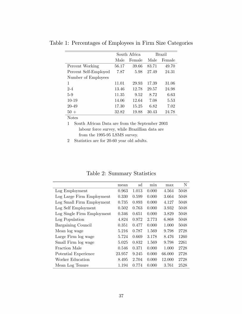
Table 1: Percentages of Employees in Firm Size Categories

South Africa BrazilMale Female Male Female

Percent Working 56.17 39.66 83.71 49.70Percent Self-Employed 7.87 5.98 27.49 24.31Number of Employees1 11.01 29.93 17.39 31.062-4 13.46 12.78 29.57 24.985-9 11.35 9.52 8.72 6.6310-19 14.06 12.64 7.08 5.5320-49 17.30 15.25 6.82 7.0250 + 32.82 19.88 30.43 24.78Notes1 South African Data are from the September 2003

labour force survey, while Brazillian data arefrom the 1995-95 LSMS survey.

2 Statistics are for 20-60 year old adults.

Table 2: Summary Statistics

mean sd min max NLog Employment 0.963 1.013 0.000 4.564 5048Log Large Firm Employment 0.330 0.599 0.000 3.664 5048Log Small Firm Employment 0.735 0.893 0.000 4.127 5048Log Self Employment 0.502 0.763 0.000 3.932 5048Log Single Firm Employment 0.346 0.651 0.000 3.829 5048Log Population 4.824 0.972 2.773 6.868 5048Bargaining Council 0.351 0.477 0.000 1.000 5048Mean log wage 5.216 0.787 1.569 9.798 2728Large Firm log wage 5.724 0.669 3.178 8.476 1260Small Firm log wage 5.025 0.832 1.569 9.798 2261Fraction Male 0.546 0.371 0.000 1.000 2728Potential Experience 23.957 9.245 0.000 66.000 2728Worker Education 8.495 2.704 0.000 12.000 2728Mean Log Tenure 1.194 0.774 0.000 3.761 2528

37

Table 3: Firm Size by Bargaining Council Status

Among All Industries Among BargainingCouncil Industries

Firm Size Never a BC BC Industry BC absent BC presentAll 56.67 43.33 51.8 48.2Self Employed 24.67 75.33 65.94 34.06Small Firms 54.53 45.47 62.65 37.35Large Firms 59.02 40.98 30.88 69.12Notes1 Summary statistics of adults aged 20-60 in September 20032 Bargaining Council Industries are covered by a Bargaining

Council Agreement at least sometimes

Table 4: Bargaining Council Coverage

Fraction Fraction of magisterialIndustry of workers districts covered

2000 2003Fishing 0.001 0 1Textile Manufacturing 0.020 1 1Metal Product Manf 0.015 1 1Electrical Machinery Manf 0.003 1 0.91Transport Equip Manf 0.005 1 1Furniture Manf 0.011 0.831 0.827Construction 0.101 0.343 0.204Retail Trade 0.256 0.156 0.217Hotels and Restaurants 0.058 0.336 0.266Land Transport 0.019 1 1Air Transport 0.001 1 0Other Business Acts 0.053 0.22 0.191Public Service 0.030 1 1Recreational/Cultural Act 0.005 1 1Other Service Activities 0.022 0.445 0.391Notes1 Fraction of workers is the average, 2000-20032 Fraction of magisterial districts is weighted by the working

population in that industry in each magisterial district

38

Table 5: Benchmark Estimates: Difference-in-differences and Spatial RD

(1) (2) (3) (4)Dependent Variable Employment Large Firm Small Firm Self

Employment Employment Employment

Panel A: Difference-in-Difference EstimatesBargaining Council -0.070** -0.047 -0.066** -0.062*

(0.031) (0.036) (0.032) (0.033)

N 5048 5048 5048 5048Panel B: Regression Discontinuity Estimates

Bargaining Council -0.364** -0.228*** -0.303** -0.303**(0.145) (0.079) (0.145) (0.111)

Distance to the Border 0.002 0.002 0.001 0.002(0.004) (0.002) (0.004) (0.004)

Bargaining Council * -0.002 0.000 -0.002 -0.003Distance to the Border (0.007) (0.003) (0.006) (0.005)N 1451 1451 1451 1451Notes1 Presents IV estimates of the effect of bargaining council status on

several specifications.2 Columns indicate the dependent variable, while rows indicate the

sample and specification used. DC-Industry fixed effects representa difference-in-differences specification

3 Bargaining Council (BC) status is instrumented with BC eligibility;a magisterial district-industry is BC-eligible if at least one magisterialdistrict in the same district council has a BC in that industry.

4 Difference-in-Differences errors are clustered at the district council levelwhile Spatial RD errors are clustered at the district council-industry level

39

Table 6: Bargaining Council Effects on Employment

(1) (2) (3) (4) (5)Dependent Variable Employment Large Firm Small Firm Self Single Firm

Employment Employment Employment EmploymentFixed Effects LevelNone -0.081** -0.012 -0.114*** -0.100** -0.055

(0.039) (0.041) (0.038) (0.042) (0.041)Magisterial District -0.102*** -0.061 -0.119*** -0.119*** -0.048

(0.036) (0.040) (0.029) (0.039) (0.035)Magisterial District-Year -0.130*** -0.051 -0.158*** -0.149*** -0.092**

(0.044) (0.045) (0.028) (0.054) (0.041)Magisterial District-Industry -0.075** -0.051 -0.071** -0.067** -0.017

(0.032) (0.038) (0.033) (0.034) (0.022)

N 5048 5048 5048 5048 5048Notes1 Presents IV estimates of the effect of bargaining council status on several specifications.2 Each column indicates the dependent variable, while rows indicate the level of fixed

effects used. Employment numbers are measured as log (Employment+1)3 Bargaining Council (BC) status is instrumented with BC eligibility; a magisterial district-

industry is BC-eligible if at least one magisterial district in the same district councilhas a BC in that industry.

4 All errors are clustered within the industry over space and time and among all industries,magisterial districts, and years in a given district council.

40

Table 7: Wage Effects of Bargaining Councils

(1) (2) (3) (4) (5)Dependent Variable Wage Wage Small Firm Large Firm Wage

Wage WageFixed Effects Level

None 0.205** 0.216*** 0.192** 0.136 0.146***(0.091) (0.076) (0.090) (0.112) (0.048)

Magisterial District 0.141** 0.179*** 0.150** -0.062 0.140***(0.061) (0.048) (0.066) (0.121) (0.055)+

Magisterial District-Year 0.122 0.141*** 0.196*** -0.056 0.079***(0.096) (0.049) (0.068) (0.145) (0.026)

Magisterial District-Industry 0.091 0.116 -0.069 0.085***(0.059) (0.114) (0.064) (0.030)

Radius 30 50 50 50 50Worker Composition? No No No No Yes

Sample Wage Wage Small Wage Large Wage WageN 2728 2728 2261 1260 2728

Notes1 Presents coeffi cients of Bargaining Councils on mean log wages,

and mean log wages in small or large firms.2 Rows consider different fixed effects.3 Bargaining Council (BC) status is instrumented with BC eligibility; a

magisterial district-industry is BC-eligible if at least one magisterialdistrict in the same district council has a BC in that industry.

4 Results are conditional on spatial-industry (with a radius given in theradius row) and time fixed effects, and a quartic in log population.

5 All errors are clustered within the industry over space and time andamong all industries, magisterial districts, and years in a given district council.

6 The + standard error is the maximum error from clustering either only amongspace or within district councils as the estimated variance was negative(following Cameron, Gelbach, and Miller 2006)

7 Column 5 includes worker gender, age, potential experience, and race controls

41

Table 8: Bargaining Council Effects by Firm Size: Low Employment Sample

(1) (2) (3) (4) (5)Dependent Variable Employment Large Firm Small Firm Self Single Firm

Employment Employment Employment EmploymentFixed Effects LevelNone -0.138** 0.009 -0.131*** -0.057 -0.046

(0.059) (0.031) (0.050) (0.047) (0.046)Magisterial District -0.155*** -0.020 -0.128*** -0.073* -0.032

(0.047) (0.023) (0.042) (0.040) (0.038)Magisterial District-Year -0.160*** -0.005 -0.139*** -0.088 -0.048

(0.058) (0.032) (0.054) (0.059) (0.053)Magisterial District-Industry -0.118*** -0.017 -0.104*** -0.047 -0.019

(0.041) (0.022) (0.031) (0.030) (0.018)

N 3631 3631 3631 3631 3631Notes1 Presents IV estimates of the effect of bargaining council status on several specifications.2 Each column indicates the dependent variable, while rows indicate the level of fixed

effects used. Employment numbers are measured as log(Employment+1).3 Bargaining Council (BC) status is instrumented with BC eligibility; a magisterial district-

industry is BC-eligible if at least one magisterial district in the same district councilhas a BC in that industry.

4 All errors are clustered within the industry over space and time and among all industries,magisterial districts, and years in a given district council

5 Sample is restricted to magisterial district-industry observations which represent less than 20% of theemployment in that industry in that district council on average

42

Table 9: Border Jumping

Dependent Variable Employment Large Firm Small FirmEmployment Employment

(1) (2) (3) (4) (5) (6)Bargaining Council side, 0.130*** -0.094 -0.038 -0.269* 0.072 -0.01130 mile border (0.050) (0.296) (0.071) (0.152) (0.131) (0.292)

Not Bargaining Council 0.218*** 0.251** 0.150 0.059 0.185 0.244**side, 30 Mile Border (0.083) (0.098) (0.110) (0.104) (0.124) (0.103)

Bargaining Council side, 0.143 0.141 -0.078 0.105 0.174 0.12050 mile border (0.120) (0.219) (0.129) (0.158) (0.105) (0.200)

Not Bargaining Council -0.159 0.051 0.073 0.054 -0.275* -0.028side, 50 Mile Border (0.145) (0.050) (0.077) (0.033) (0.149) (0.053)

Bargaining Council -0.124** -0.004 -0.126**Agreement (0.051) (0.030) (0.062)

Fixed Effects MD- DC-Ind- MD- DC-Ind- MD- DC-Ind-Indus Year Indus Year Indus Year

N 5048 5048 5048 5048 5048 5048Notes1 Presents IV estimates of employment or employment by firm size on bargaining

council status, as well as being within 30 or 50 miles of the regime border,where the effect of being on a border is allowed to be asymmetric by whichside of the border a magisterial district is on.

2 All results are conditional on time fixed effects and a quartic in log population3 All errors are clustered within the industry over space and time and among

all industries, magisterial districts, and years in a given district council.4 DC-Ind-Year fixed effects are at the district council-industry-year level5 Bargaining Council (BC) and border status are instrumented with BC and border

eligibility; a magisterial district-industry is eligible if at least one magisterialdistrict in the same district council has a BC in that industry. It is border-eligible if it is within k miles of a magisterial district that is BC-eligible

43

Figure 1: Regression Discontinuity Estimates

(a) Employment Residuals

−.4

−.3

−.2

−.1

0.1

.2.3

.4M

ean

Em

ploy

men

t Res

idua

ls

−100 −75 −50 −25 0 25 50 75 100distance to border

®

(b) Small Firm Employment Residuals

−.4

−.3

−.2

−.1

0.1

.2.3

.4M

ean

Sm

all F

irm E

mpl

oym

ent R

esid

uals

−100 −75 −50 −25 0 25 50 75 100distance to border

®

(c) Large Firm Employment Residuals

−.4

−.3

−.2

−.1

0.1

.2.3

.4M

ean

Larg

e F

irm E

mpl

oym

ent R

esid

uals

−100 −75 −50 −25 0 25 50 75 100distance to border

®

(d) Self Employment Residuals

−.4

−.3

−.2

−.1

0.1

.2.3

.4M

ean

Sel

f Em

ploy

men

t Res

idua

ls

−100 −75 −50 −25 0 25 50 75 100distance to border

®

Figure compares average employment residuals for various firm sizes against distances tothe border of a bargaining council regime, in miles. Positive distances indicate that thetown is on the covered side of the bargaining council border (i.e. that the town is covered bya bargaining council), while negative distances indicate that the town is on the uncoveredside.

44