High-Temperature Superconductors as Electromagnetic...

1

High-Temperature Superconductors as Electromagnetic Deployment and Support Structures in Spacecraft

Gwendolyn Vines Gettliffe, David W. Miller

December 2012 SSL # 14-12

3


Gwendolyn Vines Gettliffe, David W. Miller

December 2012 SSL # 14-12

This work is based on the unaltered text of the thesis by Gwendolyn Vines Gettliffe submitted to the Department of Aeronautics and Astronautics in partial fulfillment of the requirements for the degree of Master of Science at the Massachusetts Institute of Technology.

5


by

Gwendolyn Vines Gettliffe

Submitted to the Department of Aeronautics and Astronautics on December 12, 2012, in partial fulfillment of the

requirements for the degree of Master of Science in Aeronautics and Astronautics

Abstract In this thesis, we investigate a new structural and mechanical technique aimed at reducing the mass and increasing the stowed-to-deployed ratio of spacecraft systems. This technique uses the magnetic fields generated by high-temperature superconductors (HTSs) to support spacecraft structures and deploy them to operational configurations from stowed positions inside a launch vehicle fairing. The chief limiting factor in spacecraft design today is the prohibitively large launch cost per unit mass. Therefore, the reduction of spacecraft mass has been a primary design driver for the last several decades. Traditionally, spacecraft mass reduction occurs through the use of isogrid panels, aluminum or composites, and inflatable beams all reduce the mass of material necessary to build a truss or apply surface forces to a spacecraft structure. We instead look at using electromagnetic body forces generated by HTSs to reduce the need for material, load bearing support, and standoffs on spacecraft by maintaining spacing, stability, and position of elements with respect to one another.

The objective of this thesis is to conduct an initial feasibility study for the use of HTS coils as deployment and support elements in spacecraft structures. To accomplish this objective, we have developed the equations of motion for coils responding to electromagnetic forces while under the influence of constraining elements (i.e. tethers and hinged panels) and validated numerical models of these equations against known analytical solutions. By nondimensionalizing the equations of motion, we have been able to reduce our design variable space through the introduction of lumped dimensionless parameters. This enables simpler trade analysis with regards to structure deployment time and equilibrium configuration, the results of which are also presented and discussed. On the basis of these analyses, we provide suggestions for the selection of design values to achieve desired structural characteristics.

Finally, we have introduced, and discussed on the basis of our modeling results, the viability of HTS structures in the context of trade analyses. Trades were described at the mission level, the structural subsystem level, and the component level against traditional and more recently developed alternative structural technologies.

Thesis Supervisor: David W. Miller Title: Professor of Aeronautics of Astronautics

6

Acknowledgments

This work was performed primarily under Grant No. 1122374 with the National Science Foundation as part of the Graduate Research Fellowship program. The work was also performed for contract NNX11AR35G, High-Temperature Superconductors as Electromagnetic Deployment and Support Structures in Spacecraft, with the NASA Innovative Advanced Concepts Program. The author gratefully thanks the sponsors for their generous support that enabled this research. The author also thanks Niraj Inamdar for contributions to Chapter 3.

7

Table of Contents

Abstract ........................................................................................................................................ 5

Acknowledgments........................................................................................................................ 6

List of Figures ............................................................................................................................... 9

List of Tables .............................................................................................................................. 11

1 Chapter 1 - Introduction ...................................................................................................... 12

1.1 Motivation ................................................................................................................. 12

1.1.1. Reduced mass .................................................................................................... 13

1.1.2. Larger structures with same launch vehicles ..................................................... 17

1.1.3. Vibration- and thermally-isolated structures .................................................... 19

1.1.4. Staged deployment, in-space assembly, and partial system replacements ...... 20

1.1.5. Reconfiguration of structures after deployment ............................................... 20

1.2 Study objectives/Research questions ....................................................................... 21

1.3 Thesis roadmap ......................................................................................................... 24

2 Chapter 2 – Background....................................................................................................... 26

2.1 Scientific principles enabling HTS structures ............................................................ 26

2.1.1 Generation of Lorentz and Laplace forces ......................................................... 26

2.1.2 Meissner effect, superconductors, and manufacturing of HTS wire ................. 27

2.1.3 Space environment ............................................................................................ 30

2.2 Enabling technology and previous work ................................................................... 31

2.2.1 Dynamics and control ........................................................................................ 34

2.2.2 Thermal control ................................................................................................. 38

2.3 Technology readiness ................................................................................................ 40

3 Chapter 3 – Theoretical Approach and Model Design ......................................................... 41

3.1 Dynamics of unrestrained coils ................................................................................. 41

3.1.1 Translational motion .......................................................................................... 41

3.1.2 Rigid body dynamics and rotation ..................................................................... 44

3.2 Incorporation of constraining elements.................................................................... 45

3.2.1 Tethers ............................................................................................................... 46

3.2.2 Hinges ................................................................................................................. 54

3.3 Dynamic model implementation ............................................................................... 61

3.3.1 General solution algorithm ................................................................................ 61

8

3.3.2 Note on solution of stiff equations .................................................................... 65

3.4 Validation of numerical models ................................................................................ 66

3.4.1 Analytic dipole model ........................................................................................ 66

3.4.2 Sources of error in numerical approximation .................................................... 67

3.4.3 Validation models .............................................................................................. 69

3.4.4 Validation results ............................................................................................... 72

3.4.5 Note on elasticity of panel ................................................................................. 81

3.4.6 Motion of a coil under its own force in Expand configuration .......................... 82

3.5 Conclusion ................................................................................................................. 84

4 Chapter 4 – Feasibility .......................................................................................................... 85

4.1 Electromagnetic structure design variables .............................................................. 85

4.2 Reformulation of equations of motion for trade space analysis .............................. 87

4.3 Trades ........................................................................................................................ 92

4.3.1 Six Degree of Freedom (6DoF) free ................................................................... 93

4.3.2 Tethered constraints in Separate configuration ................................................ 95

4.3.3 Hinged constraints in Unfold configuration..................................................... 108

4.4 Conclusion ............................................................................................................... 114

5 Chapter 5: Viability ............................................................................................................ 115

5.1 Alternative structural technology trades ................................................................ 117

5.1.1 Comparison of HTS structures to alternative structural technologies ............ 119

5.2 Internal variable trades ........................................................................................... 121

5.3 Future work ............................................................................................................. 126

5.4 Summary and conclusions ....................................................................................... 128

9

List of Figures

Figure 1: Comparison of electromagnetic (EM) and aluminum (Al) beam masses .................................... 14 Figure 2: Chronological progression of net areal densities of space telescopes; mirror diameters listed

beside points ............................................................................................................................. 16 Figure 3: Launch vehicle cost in relation to orbit altitude and satellite dry mass [1] ................................ 17 Figure 4: Roadmap of the chapters of this thesis, in inclusion order (big blue arrows) and with subject

tie-ins (small arrows) ................................................................................................................. 24 Figure 5: Critical surface for Type II superconductor [3] ............................................................................ 28 Figure 6: Cutaway view of a 2G HTS wire [6] .............................................................................................. 29 Figure 7: 15-strand HTS Roebel cable [7] .................................................................................................... 30 Figure 8: Concept for a Next Next Generation Space Telescope using several of the proposed uses of

electromagnets on a spacecraft ................................................................................................ 32 Figure 9: MIT SSL EMFF Testbed [12] ......................................................................................................... 35 Figure 10: A SPHERE outfitted with RINGS hardware in laboratory ........................................................... 36 Figure 11: Cross-section of heat pipe (left) and cryogenic heatpipe (copper casing) in open toroidal

vacuum chamber (right)............................................................................................................ 38 Figure 12: Two-part composite heatpipe showing an HTS coil inside ........................................................ 39 Figure 13: An unrestrained two coil system, viewed slightly off-axis, showing variables used in the

computation of electromagnetic force using the Biot-Savart law ............................................ 42 Figure 14: Diagram of 3-tether spacing between two coils ........................................................................ 46 Figure 15: Diagram of 2-tether spacing and unrestricted motion .............................................................. 46 Figure 16: Conceptual illustration of electromagnetic, elastic tether, and damping forces in tethered

deployment when tethers are taut or stretched ...................................................................... 47 Figure 17: Three coil Separate configuration with slack tethers ................................................................ 49 Figure 18: Graphical depiction of tether and tether endpoint dimensions in a two coil system .............. 50 Figure 19: Visualization of elastic forces and dimensions used in calculating elastic forces and torques in

a two-coil system ...................................................................................................................... 50 Figure 20: Two coils repelling each other across a hinge in Unfold configuration ..................................... 54 Figure 21: Conceptual illustration of directional effects of electromagnetic, spring, and damping torques

in hinge deployment ................................................................................................................. 55 Figure 22: Hinged panels at equilibrium angle of spring (solid coils) and at stretched angle (dotted coils)

with panel dimension definitions and torsional spring ............................................................ 56 Figure 23: Hinged panels at equilibrium angle of spring (solid coils) and at stretched angle (dotted coils)

with angle definitions and torsional spring .............................................................................. 58 Figure 24: Net rotation of hinge pair around hinge axis over time, solid coils starting position at time t,

dotted coils position at time t+1 ............................................................................................... 59 Figure 25: Rigid coil functional configurations............................................................................................ 61 Figure 26: Tether Simulink model block diagram, shown with outputs of electromagnetic force, elastic

tether force, and damping force. .............................................................................................. 63 Figure 27: Hinge Simulink model block diagram, shown with outputs of electromagnetic force (F12_out),

electromagnetic torque (T1,2out), torque around hinge(torque_1,2_t), and angle of panels (angle_for_1,2) at each timestep. ............................................................................................. 64

Figure 28: Proportional difference between numerical and dipole approximations ................................. 67 Figure 29: Comparison of numerical and dipole initial forces over a range of starting distances ............. 68 Figure 30: Coil separation as a function of time for Separate configuration. Spring constant is varied,

while damping coefficient is kept at the baseline value. .......................................................... 74

10

Figure 31: Coil separation as a function of time for Separate configuration. Damping coefficient is varied, while spring constant is kept at the baseline value. ................................................................. 75

Figure 32: Angular separation between hinge elements for the Unfold configuration. Hinge spring constant is varied, while torque damping coefficient is kept at the baseline value. ............... 77

Figure 33: Angular separation between hinge elements for the Unfold configuration. Torque damping coefficient is varied, while hinge spring constant is held at the baseline value. ...................... 78

Figure 34: Effect of discretization on numerical calculations. Baseline tether case is calculated for Biot-Savart/numerical and dipole force laws, with the former approximated by increasingly finer discretizations . The inset shows the same, near the oscillation peak occurring around 20 s. .................................................................................................................................................. 79

Figure 35: Expand deployment configuration ............................................................................................ 82 Figure 36: Instantaneous self force on coil for two different coil shapes. Direction and magnitude of

force indicated in arbitrary units. ............................................................................................. 83 Figure 37: Visualization of self-deployment of a coil from a stowed configuration to a planar, circular

shape. ........................................................................................................................................ 84 Figure 38: Time T to separate to 20 x * as a function of plotted for values of * from

.................................................................................................................................. 93

Figure 39: Deployment time T as a function of plotted for different values of b* from to

. .................................................................................................................................................. 96

Figure 40: Deployment time T as a function of γ plotted for different values of k* from to

. .................................................................................................................................................. 98

Figure 41: Deployment time T as a function of γ plotted for different values of from 0.5 to 5.5 coil

radii. ........................................................................................................................................ 100 Figure 42: Deployment time T as a function of γ plotted for different values of * from 5 to 10 coil radii.

................................................................................................................................................ 102 Figure 43: Deployment time T as a function of γ plotted for different values of * from 5 to 20 coil radii.

................................................................................................................................................ 103

Figure 44: Equilibrium length *as a function of γ plotted for different values of k* from to

. ....................................................................................................................................... 105

Figure 45: Equilibrium length *as a function of γ plotted for different values of * from 6 to 18 coil

radii. ........................................................................................................................................ 106 Figure 46: Equilibrium length *as a function of γ with k* fixed at baseline * and any value of b* or

. ...................................................................................................................................... 107

Figure 47: Deployment time T as a function of ξ plotted for different values of β* from to

. ....................................................................................................................................... 109

Figure 48: Deployment time T as a function of ξ plotted for different values of * from to

. .................................................................................................................................. 110

Figure 49: Deployment time T as a function of ξ plotted for different values of from to and . ....................................................................................................................... 111

Figure 50: Deployment time T as a function of ξ plotted for different values of from to and . ...................................................................................................................... 112

Figure 51: Equilibrium angle as a function of moment coefficient ξ for various κ* and = 0 and π/4.

................................................................................................................................................ 113

11

List of Tables

Table 1: Top 4 most massive subsystems average % of dry mass [2] ........................................................ 14 Table 2: Current and proposed launch vehicle specifications .................................................................... 19 Table 3: Seven potential functional coil configurations ............................................................................. 22 Table 4: Previous and ongoing work on electromagnetic functions in spacecraft ..................................... 33 Table 5: Error between numerical and dipole force calculations ............................................................... 68 Table 6: Baseline values of physical parameters for simulation ................................................................. 73 Table 7: Design variables ............................................................................................................................ 85 Table 8: Dimensionless variable definitions ............................................................................................... 88 Table 9: Dimensionless parameter definitions ........................................................................................... 90 Table 10: Subsystem advantages and disadvantages of HTS structures over traditional options ........... 116 Table 11: Description of alternative structural technologies ................................................................... 118 Table 12: Comparison of HTS structures to alternative structural technologies ...................................... 119 Table 13: Qualitative comparison of deployable structure options ......................................................... 120 Table 14: System variable trades .............................................................................................................. 122

12

1 Chapter 1 - Introduction

1.1 Motivation

This thesis, which marks the conclusion of a one-year NASA Innovative Advanced Concepts (NIAC) Phase I study, describes a new structural and mechanical technique aimed at reducing the mass and increasing the deployed-to-stowed length and volume ratios of spacecraft systems. This technique, which we call MAGESTIC (MAGnetically Enabled STructures using Interacting Coils), uses the magnetic fields generated by electrical current passing through coils of high‐temperature superconductors (HTSs) to support spacecraft structures and deploy them to operational configurations from their stowed positions inside a launch vehicle.

The chief limiting factor in accessing space today is the prohibitively large launch cost per unit mass of spacecraft. [1] As a result of large launch costs, the reduction of spacecraft mass has been a primary design driver for the last several decades. The traditional approach to the reduction of spacecraft mass is the optimization of actuators and structures to use the minimum amount of material required for support, deployment, and interconnection of spacecraft components. Isogrid panels, composite honeycomb panels, and gas-filled inflatable beams all reduce the mass of material necessary to build a truss or panel, provide separation between elements, or otherwise apply surface forces to a spacecraft structure. An alternative to these density-reducing methods is the use of electromagnetic body forces generated by HTSs to reduce the need for material, load‐bearing support, and standoffs on spacecraft by maintaining spacing, stability, and position of elements with respect to one another.

HTS structures present an opportunity for significant mass savings over traditional options, especially in larger systems that require massive structural components. Electromagnetic body forces generated by superconducting magnets are used to move and position spacecraft elements in lieu of length-spanning, tangible structural components, such as telescoping booms (Nuclear Spectroscopic Telescope Array, or NuSTAR), segmented beams (James Webb Space Telescope, or JWST) and inflatables (Echo-1). Because of the way in which HTS structures gain mass in discrete packages (the addition of coils), I hypothesize that there is a spacecraft size class wherein or above which HTS structures have less mass per unit characteristic length of the spacecraft than aluminum beams. HTS structures would therefore offer the performance benefits of larger deployed structures while enabling the stowed structure to fit into existing launch vehicle payload fairings. However, the major cost of using HTS structures is the need to cool them to low temperatures so that they become superconducting, which requires passive cooling structures like sunshields or active cooling subsystems like cryogenic heat pipes. This work will also discuss the use of non-superconducting conductors for smaller forces or distances when passive cooling is not available. HTSs (which in general are superconducting at temperatures below 77K) and room-temperature conductors can be utilized in tandem to perform more complex operations.

13

We have identified several primary benefits that MAGESTIC can offer to the aerospace community: reduced mass of spacecraft, dimensionally larger structures that are able to be stowed in the same launch vehicles, structures with vibrationally and thermally isolated elements, staged deployment of spacecraft, simpler in-space assembly, partial system replacements if failure in one element occurs, and reconfigurability of structures after initial deployment. These potential benefits will be discussed in the following sections.

1.1.1. Reduced mass

HTS structures can change the way mass scales with size; above some characteristic size for each spacecraft structure, the HTS system weighs less than other methods. This is because while the mass of a beam, for instance, with density , increases continuously across a length L as:

∫

(1.1)

the mass of an example electromagnetic “beam” mostly increases discretely, adding a coil unit of mass M (the coil plus any supporting thermal hardware) every X meters N times, where X x N = L. The electromagnetic system requires a coil at either end of the structure, however, so there are N+1 coils in the L length system. The mass of the equivalent length electromagnetic beam in this thought problem is thus approximately:

M x (N+1) = M[(L/X) + 1]. (1.2)

The two systems have comparable mass when:

(1.3)

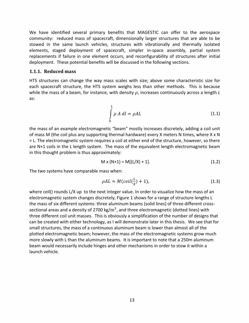
where ceil() rounds L/X up to the next integer value. In order to visualize how the mass of an electromagnetic system changes discretely, Figure 1 shows for a range of structure lengths L the mass of six different systems: three aluminum beams (solid lines) of three different cross-sectional areas and a density of 2700 kg/ , and three electromagnetic (dotted lines) with three different coil unit masses. This is obviously a simplification of the number of designs that can be created with either technology, as I will demonstrate later in this thesis. We see that for small structures, the mass of a continuous aluminum beam is lower than almost all of the plotted electromagnetic beam; however, the mass of the electromagnetic systems grow much more slowly with L than the aluminum beams. It is important to note that a 250m aluminum beam would necessarily include hinges and other mechanisms in order to stow it within a launch vehicle.

14

Figure 1: Comparison of electromagnetic (EM) and aluminum (Al) beam masses

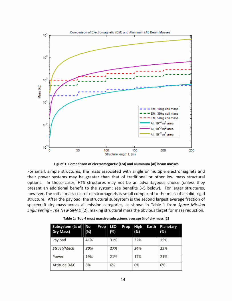
For small, simple structures, the mass associated with single or multiple electromagnets and their power systems may be greater than that of traditional or other low mass structural options. In those cases, HTS structures may not be an advantageous choice (unless they present an additional benefit to the system; see benefits 3-5 below). For larger structures, however, the initial mass cost of electromagnets is small compared to the mass of a solid, rigid structure. After the payload, the structural subsystem is the second largest average fraction of spacecraft dry mass across all mission categories, as shown in Table 1 from Space Mission Engineering - The New SMAD [2], making structural mass the obvious target for mass reduction.

Table 1: Top 4 most massive subsystems average % of dry mass [2]

Subsystem (% of Dry Mass)

No Prop (%)

LEO Prop (%)

High Earth (%)

Planetary (%)

Payload 41% 31% 32% 15%

Struct/Mech 20% 27% 24% 25%

Power 19% 21% 17% 21%

Attitude D&C 8% 6% 6% 6%

15

One goal of our work, in line with the analysis in Figure 1, is to determine at what size HTS structural options become less massive than alternative structures. In order to compare the different alternatives, we define linear structural density as being the mass of the structural subsystem (including the mass of those elements of the electrical and thermal subsystems dedicated to structural deployment and support) divided by the length of the structure (for long, thin structures like booms) and areal structural density as being the mass of the structural subsystem divided by the area of the structure (for large, broad structures, like sunshields). In contrast, the term net areal density is used in this work to refer to the total mass of a spacecraft per unit area of a specific characteristic structure, the area of which dictates a key performance parameter of the mission, such as the primary mirror of a telescope. Examining the net areal density of space telescopes over time reveals an unsurprising trend over time towards larger mirrors with lower areal densities. This trend is shown in Figure 2, which plots several extant reflecting space telescopes (Hubble, Spitzer, Kepler, Herschel) as well as one that is in development (JWST) on axes of primary mirror diameter and net areal density, with contours of constant net areal density from the top (orange) line of 1600 kg/m^2 to the lowest line (grey) of 200 kg/m^2. What we can see in this image is a trend of telescopes decreasing in net areal density both in chronological order and as mirror diameter increases. A “Next Next Generation Telescope” is plotted to show the progression into the future of decreasing areal density and increasing structural size.

16

Figure 2: Chronological progression of net areal densities of space telescopes; mirror diameters listed beside points

17

The James Webb Space Telescope (JWST) is the first space telescope being built with a primary mirror larger than the diameter of its intended launch vehicle and, as such, the mirror must be hinged, folded, and then deployed from its stowed position within the launch vehicle. As the available launch vehicle fleet remains relatively static in fairing size over the foreseeable future, larger space structures will require additional deployments in order to fit inside the fairing envelope, which suggests another potential benefit of HTS structures: the ability to stow volumetrically larger structures in the existing launch vehicle fleet. 1.1.2. Larger structures with same launch vehicles

Many space structures have performance benefits at larger sizes, but spacecraft size is limited by fairing envelope dimensions and maximum takeoff weight of launch vehicles. The high compaction ratio of HTS structures (related to how the stowed dimensions compare with the fully-deployed size of the spacecraft) could allow spacecraft designers to reap the benefits of larger structures while being less size-limited by the launch vehicle. For instance, a stack of HTS coils and tethers that can deploy to a boom length of tens of meters may be less than a meter in stowed stack height, whereas aluminum beams can only be as long as the maximum dimension of the fairing envelope before requiring hinges and actuators.

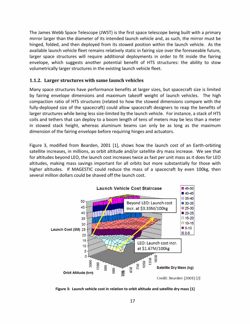
Figure 3, modified from Bearden, 2001 [1], shows how the launch cost of an Earth-orbiting satellite increases, in millions, as orbit altitude and/or satellite dry mass increase. We see that for altitudes beyond LEO, the launch cost increases twice as fast per unit mass as it does for LEO altitudes, making mass savings important for all orbits but more substantially for those with higher altitudes. If MAGESTIC could reduce the mass of a spacecraft by even 100kg, then several million dollars could be shaved off the launch cost.

Figure 3: Launch vehicle cost in relation to orbit altitude and satellite dry mass [1]

18

The performance metrics of several spacecraft components are directly related to their dimensional size. Some example performance benefits of bigger structures are given below.

Larger primary telescope mirrors can observe objects farther away because of finer angular resolution and increased effective aperture.

(1.4)

The above equation shows the relationship between diffraction-limited angular resolution Θ, wavelength λ, and aperture diameter D for a circular aperture. Angular resolution in the telescope case is the minimum angle between distinguishable objects in the image produced by the telescope’s objective, or primary mirror, which serves as the aperture when using the above equation. The larger D is, the smaller sin Θ is, which for small angles means a smaller Θ, thus giving a finer angular resolution and the ability to distinguish smaller distances in the telescope’s image, unless the payload’s resolution is otherwise limited by the design of the focal plane sensor.

Larger solar sails provide more thrust via greater surface area over which solar pressure acts.

Larger parabolic radio frequency antennas have higher gain and can enable more distant missions or increased transmission data rates.

(1.5)

where is the antenna efficiency, is the wavelength of the signal being transmitted, and A is the effective antenna area. Gain varies directly with A.

Larger solar panels can hold more photovoltaic cells and thus generate more power.

Longer synthetic aperture radar arrays achieve finest resolution in both cross- and along-track dimensions by minimizing along-track (AT) dimension and maximizing cross-track (CT) dimension.

Larger sunshields can keep more (or bigger) equipment cold.

19

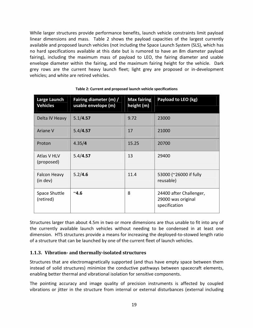
While larger structures provide performance benefits, launch vehicle constraints limit payload linear dimensions and mass. Table 2 shows the payload capacities of the largest currently available and proposed launch vehicles (not including the Space Launch System (SLS), which has no hard specifications available at this date but is rumored to have an 8m diameter payload fairing), including the maximum mass of payload to LEO, the fairing diameter and usable envelope diameter within the fairing, and the maximum fairing height for the vehicle. Dark grey rows are the current heavy launch fleet; light grey are proposed or in-development vehicles; and white are retired vehicles.

Table 2: Current and proposed launch vehicle specifications

Large Launch Vehicles

Fairing diameter (m) / usable envelope (m)

Max fairing height (m)

Payload to LEO (kg)

Delta IV Heavy 5.1/4.57 9.72 23000

Ariane V 5.4/4.57 17 21000

Proton 4.35/4 15.25 20700

Atlas V HLV (proposed)

5.4/4.57 13 29400

Falcon Heavy (in dev)

5.2/4.6 11.4 53000 (~26000 if fully reusable)

Space Shuttle (retired)

~4.6 8 24400 after Challenger, 29000 was original specification

Structures larger than about 4.5m in two or more dimensions are thus unable to fit into any of the currently available launch vehicles without needing to be condensed in at least one dimension. HTS structures provide a means for increasing the deployed-to-stowed length ratio of a structure that can be launched by one of the current fleet of launch vehicles. 1.1.3. Vibration- and thermally-isolated structures

Structures that are electromagnetically supported (and thus have empty space between them instead of solid structures) minimize the conductive pathways between spacecraft elements, enabling better thermal and vibrational isolation for sensitive components.

The pointing accuracy and image quality of precision instruments is affected by coupled vibrations or jitter in the structure from internal or external disturbances (external including

20

gravity gradient torqueing and solar pressure). Longer structures have a greater displacement at their far end than do shorter structures for the same angle rotation. Longer structures also have a lower fundamental frequency, which is undesirable due to potential coupling with the launch vehicle during launch and with the attitude control system during operations. Attitude control of the spacecraft becomes much more difficult when the fundamental frequency is low, because low frequency modes are more easily excited by attitude control systems like reaction wheels.

The cryocoolers used with cryogenic heatpipes for cooling superconducting coils generate their own disturbance profiles, so vibrational isolation would be simpler in systems already possessing passive areal cooling in the form of a sun- or heatshield. Areal cooling here refers to the cooling of an area (the area behind the shield) versus a single point on the spacecraft (ae with a cryocooler/cold finger).

1.1.4. Staged deployment, in-space assembly, and partial system replacements

Staged deployment is defined here as the ability to launch parts of a spacecraft at different times or on different launch vehicles. In-space assembly is the assembly of separate components in orbit and would be a required ability for staged deployment. Partial system replacements are when a single spacecraft element fails, another of just that component (and not the whole spacecraft) could be launched and replaced.

In combination with electromagnetic formation flight (discussed in greater detail in Section 0), HTS structures minimize or eliminate connections between spacecraft parts such that a sunshield and a mirror assembly of a spacecraft like JWST, for instance, do not have to be launched at the same time. Additionally, the entire spacecraft would not have to be replaced should one of the two fail because the parts are independent and do not require much or any physical assembly. This could give large, complex spacecraft longer lifetimes and the ability to be serviced or replaced at distances as great as Earth-Sun L2.

1.1.5. Reconfiguration of structures after deployment

Reconfigurability is the ability of a spacecraft to assume another, different operational shape after initial deployment. It is a spacecraft function that is not currently cost effective since two different functional designs on a single vehicle require a large amount of additional structural/mechanism mass, and the benefits are usually not worth the added design complexity. HTS structures allow for dynamic changes in boom length, solar array placement, and sunshield angle, as well as reversible deployments in some configurations. The capability to reconfigure could create a whole new paradigm of multi-purpose spacecraft. Much of the analysis done in Chapter 4 supports the capabilities of HTS structures for reconfiguring spacecraft in the ways mentioned above, and while HTS structures carry a significant power and thermal burden in their use, in large, high-performance systems, unique capabilities like reconfigurability might be worth the trade, especially in designs where the coils do not have to be superconducting and in use at all times. This thesis aims to provide information about the potential of HTS structures for such unique functions as well as information about the feasibility of HTS structures overall.

21

1.2 Study objectives/Research questions

The three major questions that this thesis addresses explore the technical feasibility of HTS structures, the spectrum of viable applications to spacecraft, and the new operations enabled or made substantially more realistic by HTS structures.

Question 1: Can we use electromagnetic forces generated by and acting between high-temperature superconductor current-carrying coils to move, unfold, and support parts of a spacecraft from its stowed position?

In order to answer that question, we first define functional configurations of coils that can be used to perform specific operations onboard a spacecraft. The metrics that we use to define a configuration are degrees of freedom, starting and ending positions, number of coils, and whether they are done at initial deployment of a structure or at a point later in the operational lifetime (expressed as “deployment” or “operational” phase).

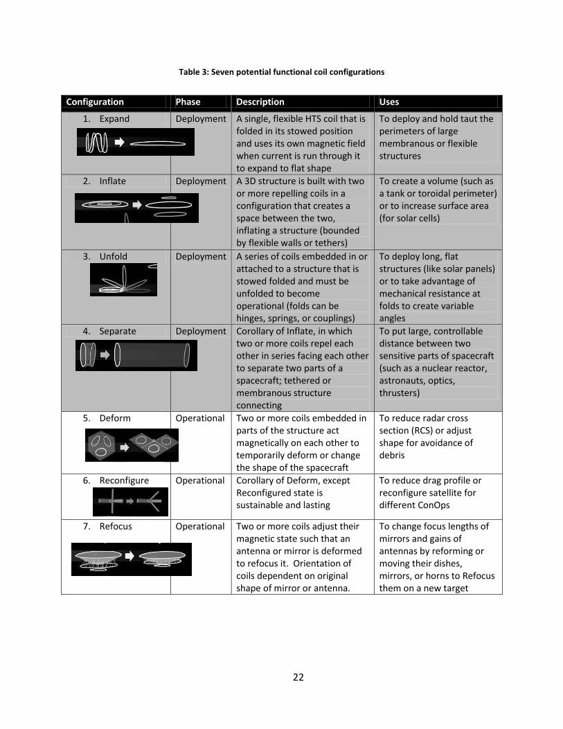
HTS coils can repel, attract, and even shear with respect to one another; in a flexible, non-circular coil, elements of the same coil can perform these actions on one another, deforming the shape of the coil over time. In combination with various boundary conditions, these operations lead to seven functional coil configurations, depicted in Table 3, that we have identified for use in spacecraft deployment and support activities. Four (1-4, in grey) are for initial deployment and three (5-7, in white) are variants of the deployment configurations for use in overall spacecraft shape change during the spacecraft operational lifetime. Table 3 describes the configurations and the spacecraft operations they could perform. These configurations will be capitalized when the configuration is being referred to in this thesis.

22

Table 3: Seven potential functional coil configurations

Configuration Phase Description Uses

1. Expand Deployment A single, flexible HTS coil that is folded in its stowed position and uses its own magnetic field when current is run through it to expand to flat shape

To deploy and hold taut the perimeters of large membranous or flexible structures

2. Inflate Deployment A 3D structure is built with two or more repelling coils in a configuration that creates a space between the two, inflating a structure (bounded by flexible walls or tethers)

To create a volume (such as a tank or toroidal perimeter) or to increase surface area (for solar cells)

3. Unfold Deployment A series of coils embedded in or attached to a structure that is stowed folded and must be unfolded to become operational (folds can be hinges, springs, or couplings)

To deploy long, flat structures (like solar panels) or to take advantage of mechanical resistance at folds to create variable angles

4. Separate Deployment Corollary of Inflate, in which two or more coils repel each other in series facing each other to separate two parts of a spacecraft; tethered or membranous structure connecting

To put large, controllable distance between two sensitive parts of spacecraft (such as a nuclear reactor, astronauts, optics, thrusters)

5. Deform Operational Two or more coils embedded in parts of the structure act magnetically on each other to temporarily deform or change the shape of the spacecraft

To reduce radar cross section (RCS) or adjust shape for avoidance of debris

6. Reconfigure Operational Corollary of Deform, except Reconfigured state is sustainable and lasting

To reduce drag profile or reconfigure satellite for different ConOps

7. Refocus Operational Two or more coils adjust their magnetic state such that an antenna or mirror is deformed to refocus it. Orientation of coils dependent on original shape of mirror or antenna.

To change focus lengths of mirrors and gains of antennas by reforming or moving their dishes, mirrors, or horns to Refocus them on a new target

23

The four deployment configurations (1-4 in Table 3) are numerically modeled in MATLAB and Simulink to verify that the deployments can be performed as described in Table 3 and are validated in the far-field (where the coils are very far apart from one another) against the dipole approximation of coil forces and torques. Chapter 3 describes these models and how they were constructed and validated.

Question 2: For which operations does this technology represent an improvement over existing or in-development options?

In order to investigate the performance of HTS structures versus other low-mass structural technologies, the ranges of performance metrics over which HTS structures are feasible and viable options for spacecraft design must first be determined. Chapter 4 characterizes the performance of HTS structures using the models introduced in Chapter 3, while in Chapter 5 they are compared to other structural options, both “traditional” rigid metal structures and “alternative” structures made with different materials (composites, ceramics, membranes, etc) and deployment operations.

Question 3: What new mission capabilities does this technology enable?

The Reconfigure, Deform, and Refocus operational configurations all represent mission capabilities that have heretofore required structures and mechanisms that are too expensive in metrics like mass, size, or power or are too complex and therefore too risky to justify for the additional performance benefits that they offer. This is why spacecraft do not commonly include these capabilities.

Using magnetic forces, however, such shape-changing mission capabilities are not structurally much different from the deployment and support configurations required to move from a stowed configuration to a deployed one, so including the ability to Reconfigure or Deform utilizes the existing structural architecture more efficiently than in non-electromagnetic structures. Operational configurations will be discussed further in Chapters 3 and 4.

The goal of this thesis to provide analyses of the dynamics of rigid (and, briefly, flexible) electromagnetic coils when exerting forces and torques on one another, such that we can support a positive answer for Question 1, narrow down the field of potential deployment and support functions that are worth further study for Question 2, and explore new spacecraft architectures that have never been implemented for Question 3.

24

1.3 Thesis roadmap

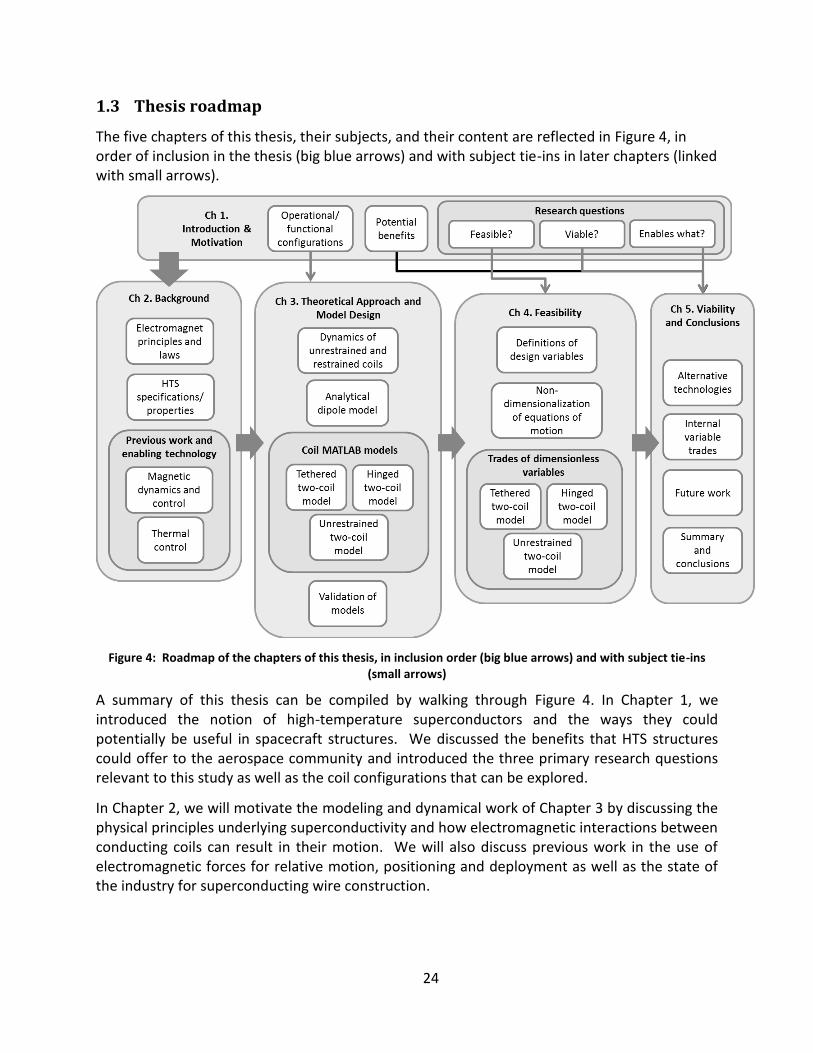
The five chapters of this thesis, their subjects, and their content are reflected in Figure 4, in order of inclusion in the thesis (big blue arrows) and with subject tie-ins in later chapters (linked with small arrows).

Figure 4: Roadmap of the chapters of this thesis, in inclusion order (big blue arrows) and with subject tie-ins (small arrows)

A summary of this thesis can be compiled by walking through Figure 4. In Chapter 1, we introduced the notion of high-temperature superconductors and the ways they could potentially be useful in spacecraft structures. We discussed the benefits that HTS structures could offer to the aerospace community and introduced the three primary research questions relevant to this study as well as the coil configurations that can be explored.

In Chapter 2, we will motivate the modeling and dynamical work of Chapter 3 by discussing the physical principles underlying superconductivity and how electromagnetic interactions between conducting coils can result in their motion. We will also discuss previous work in the use of electromagnetic forces for relative motion, positioning and deployment as well as the state of the industry for superconducting wire construction.

25

In Chapter 3, we will develop the equations of motion for coils responding to electromagnetic forces while under the influence of constraining elements (i.e. tethers and hinged panels) and validate numerical models of these equations against known analytical solutions.

In Chapter 4, we will show how we can reduce the size of the electromagnetic design trade space by modifying our equations of motion for trade analysis by nondimensionalizing them and introducing several dimensionless parameters that encode many of our design variables. We will present the results of numerous simulations using the numerical models introduced in Chapter 3.

In Chapter 5, we will discuss on the basis of the results from Chapter 4 the viability of HTS structures in the context of trade analyses. Trades will be described at the mission level, the structural subsystem level, and the component level. We will discuss future work and the conclusions we have made from the work presented in this thesis.

26

2 Chapter 2 – Background

This chapter introduces the foundational scientific principles for HTS and reviews previous development efforts to mature key enabling technologies for HTS electromagnetic structures. We discuss the enabling scientific principles and phenomena that form the basis of our study, draw lines between HTS structures and previous space electromagnetic work, and briefly examine the maturity of the HTS structure concept.

2.1 Scientific principles enabling HTS structures

HTS structures are enabled by the fundamental scientific principles of electromagnetism, the unique environment of space, and the developments made over the last several decades in manufacturing superconductors and controlling electromagnets onboard multi-system vehicles. The industry development is explored in later sections; this section describes the underlying fundamental scientific principles that enable HTS structures, including:

1. The creation of Lorentz and Laplace forces via interaction of a magnetic field and current

2. The Meissner effect, superconductivity, and the manufacturing of HTS wire 3. Enabling characteristics of space environment (microgravity and vacuum)

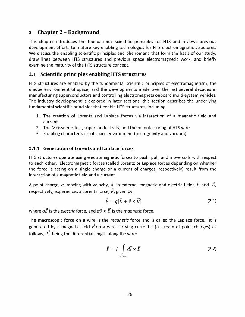
2.1.1 Generation of Lorentz and Laplace forces

HTS structures operate using electromagnetic forces to push, pull, and move coils with respect to each other. Electromagnetic forces (called Lorentz or Laplace forces depending on whether the force is acting on a single charge or a current of charges, respectively) result from the interaction of a magnetic field and a current.

A point charge, q, moving with velocity, , in external magnetic and electric fields, and ,

respectively, experiences a Lorentz force, , given by:

(2.1)

where q is the electric force, and q is the magnetic force.

The macroscopic force on a wire is the magnetic force and is called the Laplace force. It is

generated by a magnetic field on a wire carrying current (a stream of point charges) as

follows, being the differential length along the wire:

∫

(2.2)

27

The magnetic force is thus orthogonal to the wire and to the orientation of the magnetic field at

the point of calculation. In order to calculate the magnetic field for use in determining the Laplace force on a wire or coil of wire, one can use the Biot-Savart law, which can be derived

from Ampère's law and Gauss’s law, to compute the resultant magnetic field vector at a position r with respect to a steady current I (with being the magnetic constant, ) :

∫

| |

(2.3)

In the deployment modeling work that will be described in Chapter 3, the magnetic field and the Laplace forces across a current-carrying wire are approximated over time by implementing the Biot-Savart law numerically, discretizing electric current elements in order to determine the magnetic field generated by arbitrary configurations of rigid (meaning a fixed, non-changing shape) and flexible coils. Knowledge of the magnetic field at each point in space around a current-carrying wire allows the calculation of the resultant force upon another current-carrying wire as a result of that magnetic field, which can then be used to determine the number of turns a coil requires or how much current it needs to carry in order to deploy a structure. The Laplace force is used with the Biot-Savart law in this work to determine the electromagnetic forces on a coil due to the magnetic field generated by itself and other magnetic elements.

2.1.2 Meissner effect, superconductors, and manufacturing of HTS wire

Superconductors are materials that conduct electrical current perfectly below a critical temperature ; superconductors have zero resistivity, with negligible quantities right around their . Any current through them will persist significantly longer than through a non-superconductive material. Superconductivity is characterized by the Meissner effect, the expulsion of an external magnetic field from a superconductor once cooled below its during its transition to a superconducting state. Every superconductor has a critical temperature, external magnetic field strength, and current density above which superconductivity ceases, as shown graphically in Figure 5. The highest current density can be reached when the temperature and magnetic field are the lowest and vice versa for each of the axes. The critical surface represents the surface beyond which superconductivity breaks down. Superconductors enable HTS structures because they are able to generate much larger forces than standard conducting metal magnets via the superconductor’s larger current carrying capacity, which increases the distance over which superconductors can work for the same amount of mass.

28

Figure 5: Critical surface for Type II superconductor [3]

High-temperature superconductors, or HTSs, are those superconductors with s above 77K, or the boiling point of liquid nitrogen (LN2), enabling them to be cooled to a superconducting state using LN2. The higher the , the less it costs (in terms of power, storage, and consumables, for applications where a cryogen is not recycled) to do the cooling. HTS development and the subsequent development of HTS wire has led to a broad array of applications for superconductors, including long distance power transfer, electromagnets, and energy storage.

There are two types of superconductors; Type-I only exhibit the Meissner effect with one critical field strength above which superconductivity ceases. Type-II superconductors also exhibit a “mixed-state” Meissner effect that increases their critical magnetic fields and configuration stability. Type-II superconductors include all high-temperature superconductors, as well as some low-temperature superconductors (LTSs) with s too low to qualify as “high-temperature”, Because of this effect, Type-II superconductors are often used in superconducting magnets in the form of coils of wire made with superconductor filaments embedded in support material less than a millimeter in diameter.

The “mixed” Meissner effect is different from the Meissner effect in that some magnetic field penetrates the superconductor through filaments of normal-state material, and the material can support higher magnetic fields before superconductivity breaks down. There are thus two critical field strengths in Type II superconductors: beyond the first field strength, where superconductivity would cease completely in a Type I superconductor, a vortex (“mixed”) state exists in which some magnetic flux is allowed to penetrate the material while it continues superconducting. Beyond the second, higher critical field strength, superconductivity ceases.

Type-II superconductors are the only type of superconductor used in wire, because Type-I superconductors like lead, indium, and mercury typically cannot withstand fields above 0.1 T and current flow is limited to a very thin surface layer (reducing the critical current density of the material) [3]. Many superconducting wires are made with HTSs to lower cooling costs,

29

especially for non-magnetic applications. Some wire, however, especially that which is used in powerful electromagnets like those in the Large Hadron Collider, is made with LTSs that need to be kept much colder but can sustain much higher current densities than HTSs. For example, niobium–tin (Nb3Sn) has a of 18.3K and can withstand magnetic field strengths up to 30 tesla (with a record current density of 2643 A/mm^2 at 12T and 4.2K) [4]. HTS wires do not have the same current densities, and, as a result, they cannot generate magnetic fields as high as LTSs. But, though pure HTS materials are no less brittle as LTS materials, HTSs can be constructed into flexible, durable wire by depositing a thin layer on a more flexible substrate, as shown in Figure 6, or by heating a metal tube filled with powdered metals and superconductor. The flexibility of HTS wire enables the Expand configuration that we proposed earlier in this section for deployment of a single, folded and stowed coil into a large, flat, expanded coil.

Compared to standard, room-temperature conductors, HTS wires are able to create larger magnetic fields and sustain higher current densities, with little-to-no resistive losses through the wire (compared to high resistive losses in copper and aluminum). While room temperature conductor coils can be used to magnetically operate on each other, the Laplace forces generated are significantly lower than those created with HTS coils, due to the lower induced magnetic field. HTS wire thus enables electromagnetic structures with multi-meter separation between coils, which in turn enables larger vehicles and the performance benefits enumerated in Chapter 1 that accompany larger structures.

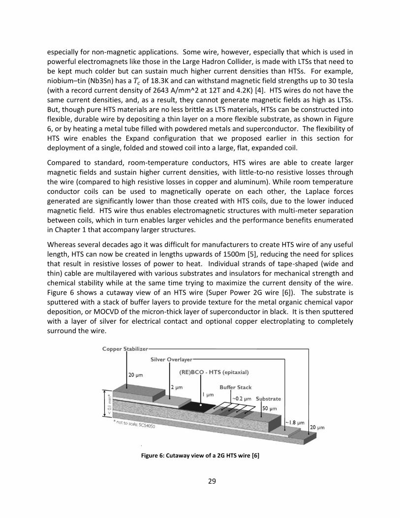
Whereas several decades ago it was difficult for manufacturers to create HTS wire of any useful length, HTS can now be created in lengths upwards of 1500m [5], reducing the need for splices that result in resistive losses of power to heat. Individual strands of tape-shaped (wide and thin) cable are multilayered with various substrates and insulators for mechanical strength and chemical stability while at the same time trying to maximize the current density of the wire. Figure 6 shows a cutaway view of an HTS wire (Super Power 2G wire [6]). The substrate is sputtered with a stack of buffer layers to provide texture for the metal organic chemical vapor deposition, or MOCVD of the micron-thick layer of superconductor in black. It is then sputtered with a layer of silver for electrical contact and optional copper electroplating to completely surround the wire.

Figure 6: Cutaway view of a 2G HTS wire [6]

30

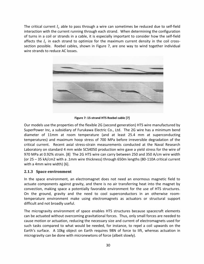
The critical current able to pass through a wire can sometimes be reduced due to self-field interaction with the current running through each strand. When determining the configuration of turns in a coil or strands in a cable, it is especially important to consider how the self-field affects the in each strand to optimize for the maximum current density in the coil cross-section possible. Roebel cables, shown in Figure 7, are one way to wind together individual wire strands to reduce AC losses.

Figure 7: 15-strand HTS Roebel cable [7]

Our models use the properties of the flexible 2G (second generation) HTS wire manufactured by SuperPower Inc, a subsidiary of Furukawa Electric Co., Ltd. The 2G wire has a minimum bend diameter of 11mm at room temperature (and at least 25.4 mm at superconducting temperatures) and maximum hoop stress of 700 MPa before irreversible degradation of the critical current. Recent axial stress-strain measurements conducted at the Naval Research Laboratory on standard 4 mm wide SCS4050 production wire gave a yield stress for the wire of 970 MPa at 0.92% strain. [8] The 2G HTS wire can carry between 250 and 350 A/cm wire width (or 25 – 35 kA/cm2 with a .1mm wire thickness) through 650m lengths (80-110A critical current with a 4mm wire width) [6].

2.1.3 Space environment

In the space environment, an electromagnet does not need an enormous magnetic field to actuate components against gravity, and there is no air transferring heat into the magnet by convection, making space a potentially favorable environment for the use of HTS structures. On the ground, gravity and the need to cool superconductors in an otherwise room-temperature environment make using electromagnets as actuators or structural support difficult and not broadly useful.

The microgravity environment of space enables HTS structures because spacecraft elements can be actuated without overcoming gravitational forces. Thus, only small forces are needed to cause motion or actuation, reducing the necessary size and current of electromagnets used for such tasks compared to what would be needed, for instance, to repel a coil upwards on the Earth’s surface. A 10kg object on Earth requires 98N of force to lift, whereas actuation in microgravity can be done with micronewtons of force (albeit slowly).

31

The vacuum of space is both beneficial and detrimental to the use of superconductors. If a thermally isolated HTS subsystem can avoid radiated input from the sun, Earth, or the space vehicle, the system can maintain superconducting temperatures without cryogens. However, it is difficult to lower the system to cryogenic temperatures in a vacuum if the system cannot be isolated from conductive (other spacecraft subsystems) or radiating (Earth, Sun, other subsystems) heat sources. This thermal environment makes more advanced cooling systems, like the cryogenic heatpipe described in Section 2.2, necessary for maintenance of the superconductor below its critical transition temperature.

2.2 Enabling technology and previous work

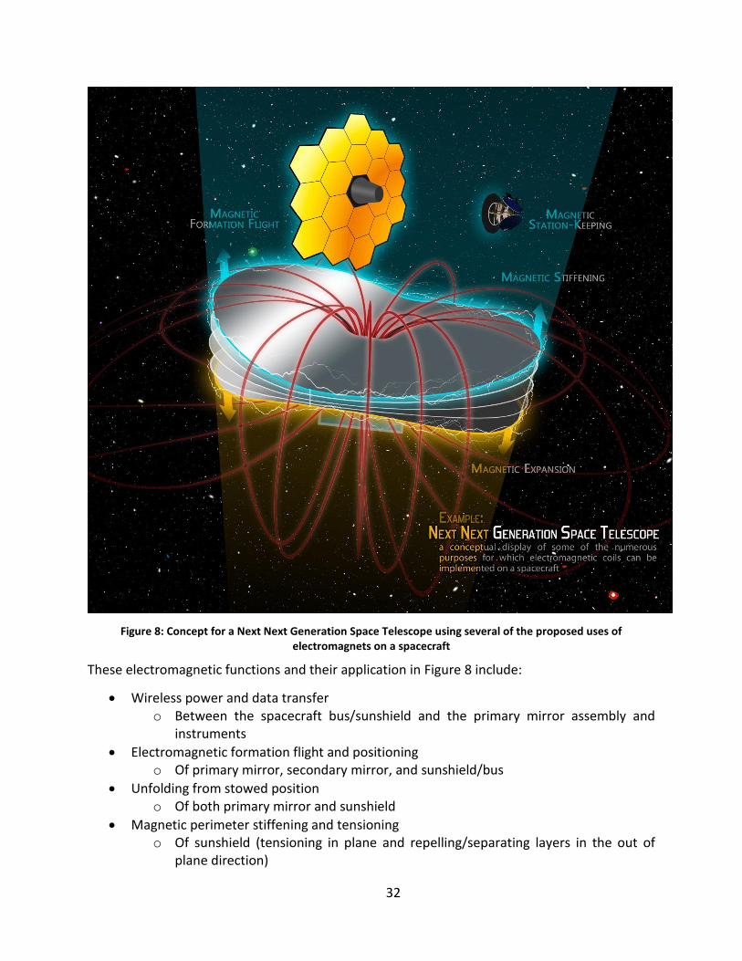
In order to more clearly visualize what has already been done in the field of electromagnetic structures, we present a concept in Figure 8 for a “Next Next Generation Space Telescope” that incorporates many of the potential functions and advantages that we see of electromagnets on large spacecraft.

32

Figure 8: Concept for a Next Next Generation Space Telescope using several of the proposed uses of electromagnets on a spacecraft

These electromagnetic functions and their application in Figure 8 include:

Wireless power and data transfer o Between the spacecraft bus/sunshield and the primary mirror assembly and

instruments

Electromagnetic formation flight and positioning o Of primary mirror, secondary mirror, and sunshield/bus

Unfolding from stowed position o Of both primary mirror and sunshield

Magnetic perimeter stiffening and tensioning o Of sunshield (tensioning in plane and repelling/separating layers in the out of

plane direction)

33

Attitude control and momentum trading between spacecraft elements o Between primary mirror assembly and sunshield o Between primary and secondary mirrors

Some advantages of the above electromagnetic functions are:

No obscuration from the secondary mirror assembly o The beams that usually position the secondary mirror in front of a primary in a

telescope assembly like JWST’s shadow the primary mirror. Removing physical connections, as in electromagnetic formation flight, removes this obscuration.

Staged deployment and element upgrades/replacements o As explained in Section 1.1.4, when physical connections are not necessary for

assembly of a structure, the deployment can be staged (different parts being launched in different launch vehicles) and spacecraft elements can be easily replaced or upgraded without complex assembly procedures.

A reduced number of deployments o A single expanding flexible coil deploying a membrane does not require four or

five different mechanisms or actions as would a mechanical deployment system. A failure of the coil would still be a major problem, but so would a failure of any of the steps in a mechanical deployment system, of which there are more

Dynamic and thermal isolation o Discussed in Section 1.1.3, formation flying elements or electromagnetically

separated structures (like the sunshield layers) have no or very limited pathways for vibration and thermal transfer.

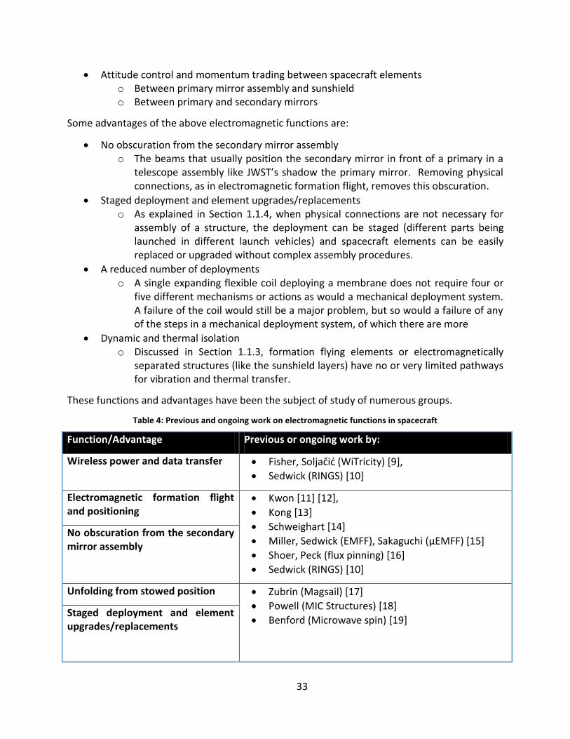
These functions and advantages have been the subject of study of numerous groups.

Table 4: Previous and ongoing work on electromagnetic functions in spacecraft

Function/Advantage Previous or ongoing work by:

Wireless power and data transfer Fisher, Soljačić (WiTricity) [9],

Sedwick (RINGS) [10]

Electromagnetic formation flight and positioning

Kwon [11] [12],

Kong [13]

Schweighart [14]

Miller, Sedwick (EMFF), Sakaguchi (μEMFF) [15]

Shoer, Peck (flux pinning) [16]

Sedwick (RINGS) [10]

No obscuration from the secondary mirror assembly

Unfolding from stowed position Zubrin (Magsail) [17]

Powell (MIC Structures) [18]

Benford (Microwave spin) [19]

Staged deployment and element upgrades/replacements

34

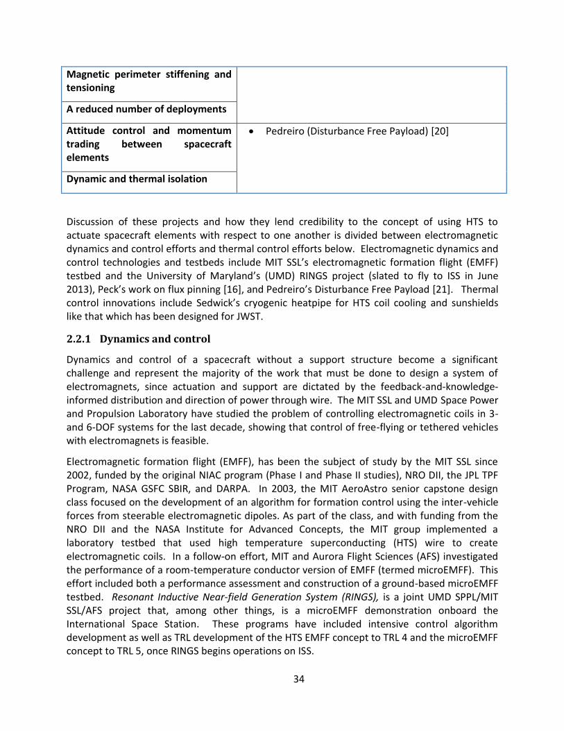
Magnetic perimeter stiffening and tensioning

A reduced number of deployments

Attitude control and momentum trading between spacecraft elements

Pedreiro (Disturbance Free Payload) [20]

Dynamic and thermal isolation

Discussion of these projects and how they lend credibility to the concept of using HTS to actuate spacecraft elements with respect to one another is divided between electromagnetic dynamics and control efforts and thermal control efforts below. Electromagnetic dynamics and control technologies and testbeds include MIT SSL’s electromagnetic formation flight (EMFF) testbed and the University of Maryland’s (UMD) RINGS project (slated to fly to ISS in June 2013), Peck’s work on flux pinning [16], and Pedreiro’s Disturbance Free Payload [21]. Thermal control innovations include Sedwick’s cryogenic heatpipe for HTS coil cooling and sunshields like that which has been designed for JWST.

2.2.1 Dynamics and control

Dynamics and control of a spacecraft without a support structure become a significant challenge and represent the majority of the work that must be done to design a system of electromagnets, since actuation and support are dictated by the feedback-and-knowledge-informed distribution and direction of power through wire. The MIT SSL and UMD Space Power and Propulsion Laboratory have studied the problem of controlling electromagnetic coils in 3- and 6-DOF systems for the last decade, showing that control of free-flying or tethered vehicles with electromagnets is feasible.

Electromagnetic formation flight (EMFF), has been the subject of study by the MIT SSL since 2002, funded by the original NIAC program (Phase I and Phase II studies), NRO DII, the JPL TPF Program, NASA GSFC SBIR, and DARPA. In 2003, the MIT AeroAstro senior capstone design class focused on the development of an algorithm for formation control using the inter-vehicle forces from steerable electromagnetic dipoles. As part of the class, and with funding from the NRO DII and the NASA Institute for Advanced Concepts, the MIT group implemented a laboratory testbed that used high temperature superconducting (HTS) wire to create electromagnetic coils. In a follow-on effort, MIT and Aurora Flight Sciences (AFS) investigated the performance of a room-temperature conductor version of EMFF (termed microEMFF). This effort included both a performance assessment and construction of a ground-based microEMFF testbed. Resonant Inductive Near-field Generation System (RINGS), is a joint UMD SPPL/MIT SSL/AFS project that, among other things, is a microEMFF demonstration onboard the International Space Station. These programs have included intensive control algorithm development as well as TRL development of the HTS EMFF concept to TRL 4 and the microEMFF concept to TRL 5, once RINGS begins operations on ISS.

35

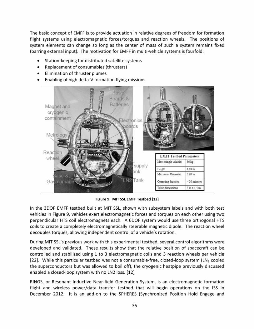
The basic concept of EMFF is to provide actuation in relative degrees of freedom for formation flight systems using electromagnetic forces/torques and reaction wheels. The positions of system elements can change so long as the center of mass of such a system remains fixed (barring external input). The motivation for EMFF in multi-vehicle systems is fourfold:

Station-keeping for distributed satellite systems

Replacement of consumables (thrusters)

Elimination of thruster plumes

Enabling of high delta-V formation flying missions

Figure 9: MIT SSL EMFF Testbed [12]

In the 3DOF EMFF testbed built at MIT SSL, shown with subsystem labels and with both test vehicles in Figure 9, vehicles exert electromagnetic forces and torques on each other using two perpendicular HTS coil electromagnets each. A 6DOF system would use three orthogonal HTS coils to create a completely electromagnetically steerable magnetic dipole. The reaction wheel decouples torques, allowing independent control of a vehicle’s rotation.

During MIT SSL’s previous work with this experimental testbed, several control algorithms were developed and validated. These results show that the relative position of spacecraft can be controlled and stabilized using 1 to 3 electromagnetic coils and 3 reaction wheels per vehicle [22]. While this particular testbed was not a consumable-free, closed-loop system (LN2 cooled the superconductors but was allowed to boil off), the cryogenic heatpipe previously discussed enabled a closed-loop system with no LN2 loss. [12]

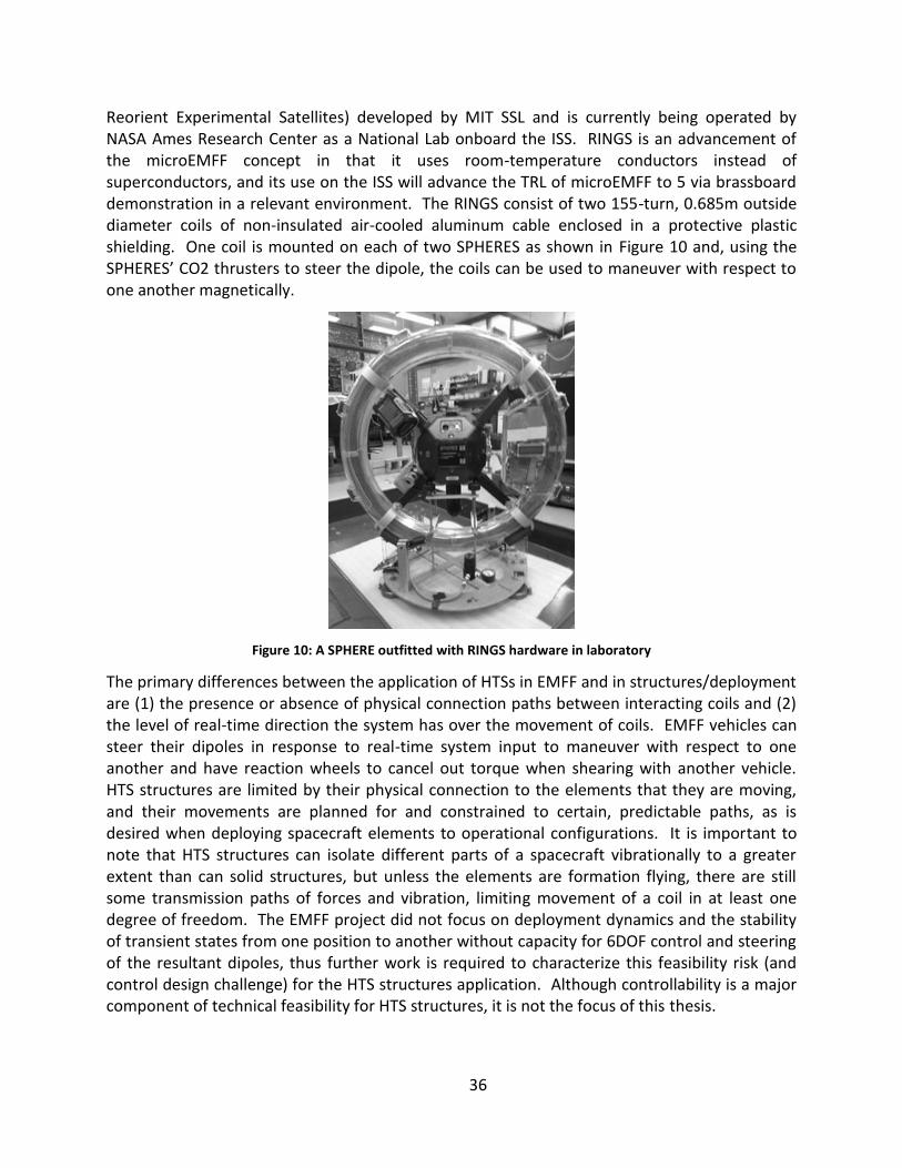
RINGS, or Resonant Inductive Near-field Generation System, is an electromagnetic formation flight and wireless power/data transfer testbed that will begin operations on the ISS in December 2012. It is an add-on to the SPHERES (Synchronized Position Hold Engage and

36

Reorient Experimental Satellites) developed by MIT SSL and is currently being operated by NASA Ames Research Center as a National Lab onboard the ISS. RINGS is an advancement of the microEMFF concept in that it uses room-temperature conductors instead of superconductors, and its use on the ISS will advance the TRL of microEMFF to 5 via brassboard demonstration in a relevant environment. The RINGS consist of two 155-turn, 0.685m outside diameter coils of non-insulated air-cooled aluminum cable enclosed in a protective plastic shielding. One coil is mounted on each of two SPHERES as shown in Figure 10 and, using the SPHERES’ CO2 thrusters to steer the dipole, the coils can be used to maneuver with respect to one another magnetically.

Figure 10: A SPHERE outfitted with RINGS hardware in laboratory

The primary differences between the application of HTSs in EMFF and in structures/deployment are (1) the presence or absence of physical connection paths between interacting coils and (2) the level of real-time direction the system has over the movement of coils. EMFF vehicles can steer their dipoles in response to real-time system input to maneuver with respect to one another and have reaction wheels to cancel out torque when shearing with another vehicle. HTS structures are limited by their physical connection to the elements that they are moving, and their movements are planned for and constrained to certain, predictable paths, as is desired when deploying spacecraft elements to operational configurations. It is important to note that HTS structures can isolate different parts of a spacecraft vibrationally to a greater extent than can solid structures, but unless the elements are formation flying, there are still some transmission paths of forces and vibration, limiting movement of a coil in at least one degree of freedom. The EMFF project did not focus on deployment dynamics and the stability of transient states from one position to another without capacity for 6DOF control and steering of the resultant dipoles, thus further work is required to characterize this feasibility risk (and control design challenge) for the HTS structures application. Although controllability is a major component of technical feasibility for HTS structures, it is not the focus of this thesis.

37

Electromagnetic actuation on spacecraft has been the subject of research by a number of groups because of its potential for vibrational isolation and reconfiguration. Disturbance Free Payload, or DFP, is an architecture developed by Pedreiro et al for use in vibration isolation achieved down to zero frequency of spacecraft payloads from the rest of the spacecraft using multiple electromagnetic actuators [21]. It improves on previous vibration isolation methods by being effective at low frequencies. DFP is not dependent on sensor characteristics and is thus exempt from sensor error. [20] DFP functions in very close proximity on the order of millimeters, however, and does not work at distances of the magnitude being discussed in this thesis (meters or larger).

Flux pinning is an electromagnetic phenomenon in superconductors that enables highly accurate positioning between an electromagnet and a permanent magnet or other magnetic field source that can be used for safer and easier in-space assembly and reconfiguration of space systems in orbit. Small defects in the superconducting material can increase critical magnetic fields and contribute to the stability of the system by fixing vortex points, or filaments, through which magnetic field lines pass and are subsequently pinned when the superconductor is cooled below its . Pinning of the field lines pins the source of the magnetic field in position and orientation. A number of joints, hinges, and interfaces can be created using configurations of permanent magnets to limit or direct the motion of a superconducting cube about the permanent magnets. As of 2009, multi-centimeter gaps between the magnets were supportable with high stiffness and damping with small masses. Flux pinning as a means of supporting and manipulating space structures is the subject of work by Peck et al at Cornell University [16].

Stiffening of membranous or low net areal density structures has been proposed on multiple occasions, such as Zubrin’s “magsail” concept in which a large membranous plasma wind sail is held taut using a flexible HTS coiled around its perimeter to repel itself into a circle and keep the sail under tension. Zubrin ultimately selected a non-magnetic deployment system (rotating booms to deploy the sail initially using centrifugal force), citing “reliable deployment” as a key issue for magsails [17]. A previous NIAC study performed by Powell et al [18] proposed a system like that being studied in this thesis: flexible cables made of high-temperature superconducting wire expanding or inflating in order to serve as deployment actuators, perimeter support, and standoff structures simultaneously for large scale spacecraft. Powell primarily discusses the HTS wire properties and materials and does not go into detail on the deployment process. This thesis will explore such magnetic deployment in detail in an effort to determine if magnetic deployment is feasible, and if so, for what types and sizes of structures.

Other past studies of deployment or support using electromagnetism in membranous structures include microwave beam‐driven spin deployment of solar sails (Benford, [19]) and membranous structures containing conductive meshes that can be shaped using magnetic pressure from permanent magnets or electromagnets (Amboss, [23]).

For applications that require long, low-mass structures, HTS structures are more suited than flux pinning or DMP to deployment and support in those situations. The possibility remains, however, of using a combination of flux pinning, DMP, EMFF, and HTS structures to magnetically assemble, deploy, and support large and complex space structures. Other light

38

structural technologies like inflatables or tensegrity structures do not have active control over their shape; they attempt to deploy and either succeed or fail, and then they passively maintain their configuration for the lifetime of the vehicle. The ability to control and change the magnetic field means that electromagnetic structures are able to change their shape after deploying, depending on their boundary conditions.

2.2.2 Thermal control

Thermal control down to cryogenic temperatures is necessary to induce superconductivity in HTSs. This level of thermal control is not normally present on spacecraft unless the vehicle has a payload that requires special cooling. Additionally, HTS performance is dictated by its warmest temperature, meaning that cooling devices are required at every point along the coil, which is not feasible (or even accomplishable), for large coils. Cooling equipment that can cool the full perimeter of a coil is needed and must be scalable to different size coils. Such equipment should preferably be consumable-free so as not to limit the lifetime of the mission. If the thermal control requires too much mass and power, the thermal subsystem could make HTS structures less competitive with traditional structures by nullifying any potential savings of HTS structures.

The cryogenic heatpipe developed by Sedwick and Kwon [12] for use in EMFF, pictured in Figure 11, provides a starting point for continued development and improvement of a competitive HTS coil cooling system by accomplishing consumable-free isothermalization to cryogenic temperatures (the same temperature at every point on the coil) with a single cryocooler.

Figure 11: Cross-section of heat pipe (left) and cryogenic heatpipe (copper casing) in open toroidal vacuum chamber (right)

This rigid heatpipe uses nitrogen as a working fluid and a stainless steel mesh as the wicking structure, with the HTS coil enclosed within the heatpipe instead of residing externally as with traditional heatpipes. A condenser, operated with an LN2 reservoir (like in the laboratory setup shown in Figure 11) or powered by a cryocooler, extracts heat from the system while the mesh passively wicks the condensed LN2 around the pipe via capillary action on several layers of wire mesh to cool and achieve isothermalization of the coil. Isothermalization means that minimal temperature gradients exist across the entire coil. Isothermal conditions are desired because the warmest point in the coil is the limiting factor in the performance of the HTS wire. When used with a cryocooler, this heatpipe is a closed system wherein the working fluid is conserved so long as the system remains sealed.

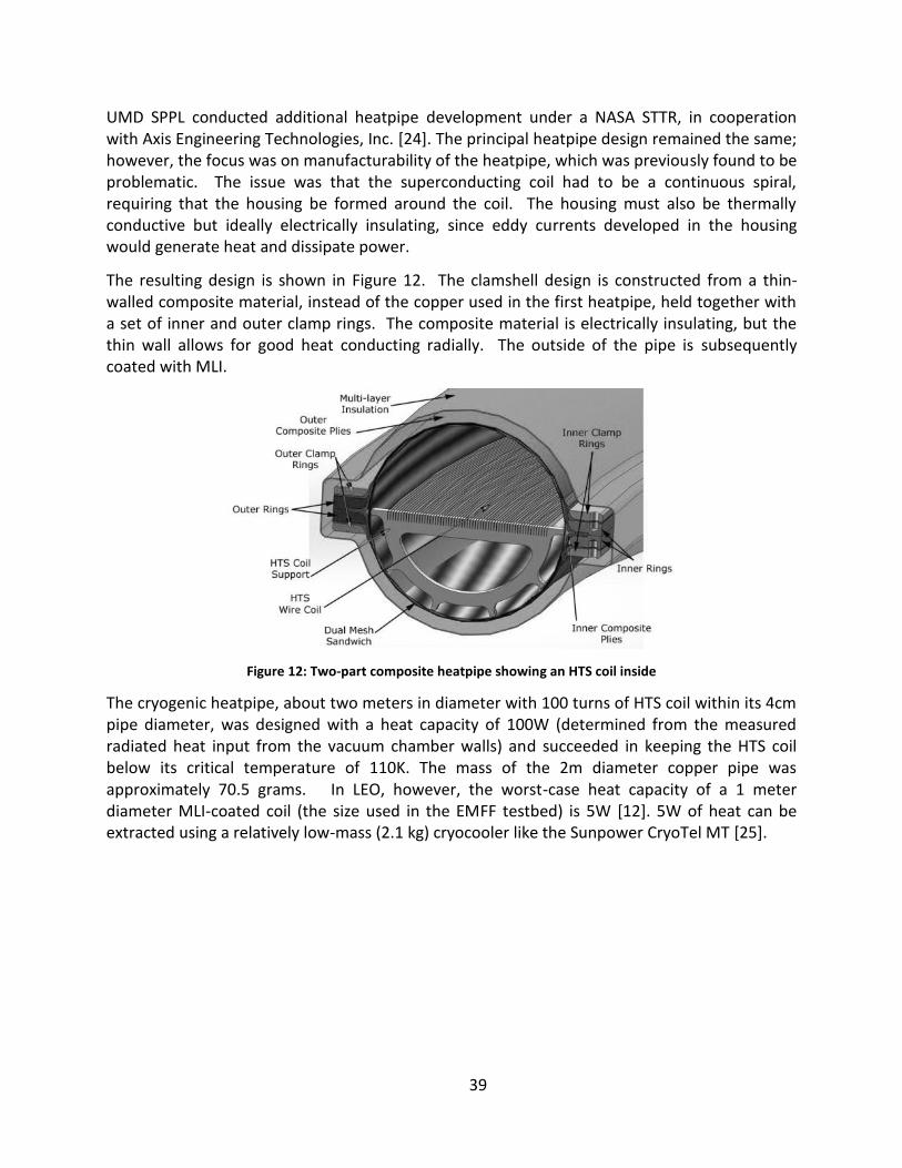
39

UMD SPPL conducted additional heatpipe development under a NASA STTR, in cooperation with Axis Engineering Technologies, Inc. [24]. The principal heatpipe design remained the same; however, the focus was on manufacturability of the heatpipe, which was previously found to be problematic. The issue was that the superconducting coil had to be a continuous spiral, requiring that the housing be formed around the coil. The housing must also be thermally conductive but ideally electrically insulating, since eddy currents developed in the housing would generate heat and dissipate power.

The resulting design is shown in Figure 12. The clamshell design is constructed from a thin-walled composite material, instead of the copper used in the first heatpipe, held together with a set of inner and outer clamp rings. The composite material is electrically insulating, but the thin wall allows for good heat conducting radially. The outside of the pipe is subsequently coated with MLI.

Figure 12: Two-part composite heatpipe showing an HTS coil inside

The cryogenic heatpipe, about two meters in diameter with 100 turns of HTS coil within its 4cm pipe diameter, was designed with a heat capacity of 100W (determined from the measured radiated heat input from the vacuum chamber walls) and succeeded in keeping the HTS coil below its critical temperature of 110K. The mass of the 2m diameter copper pipe was approximately 70.5 grams. In LEO, however, the worst-case heat capacity of a 1 meter diameter MLI-coated coil (the size used in the EMFF testbed) is 5W [12]. 5W of heat can be extracted using a relatively low-mass (2.1 kg) cryocooler like the Sunpower CryoTel MT [25].

40

2.3 Technology readiness

HTS structures are a logical evolution of the previously realized or studied applications of electromagnets in space, and they bridge the gap between electromagnetic actuation, support, and positioning as a system that is capable of all three functions. In the future, spacecraft designers can tie together many of these positioning and actuation applications into a single or collection of multiple spacecraft, utilizing formation flying, easy in-situ assembly, isolation and high stowed-to-deployed size ratio structures to enable spacecraft that have never before been possible. Therefore, in this thesis, we will address several of the questions relevant to the feasibility and viability of implementing HTS structures through modeling and trade analysis. Furthermore, a goal of this work is to mature the technology readiness level (TRL) of MAGESTIC from conceptualization and early analysis of this application (TRL 2) to a more detailed analysis and hardware proof-of-concepts (TRL 3). The work in this thesis encompasses the transition from TRL 2 to early 3 with modeling and analysis while the work that will occur during the next few years under a NASA Innovative Advanced Concepts Phase II study aims to mature the technology further through TRL 3.

41

3 Chapter 3 – Theoretical Approach and Model Design

This chapter will detail the equations of motion that describe the dynamical evolution of current-carrying coils in space and how this motion was simulated using MATLAB and Simulink models. In this thesis, we will be primarily discussing the motion of two rigid coils under a variety of boundary constraints; we will briefly discuss the motion of flexible coils in this chapter as well. These particular models were selected because between the two of them, all seven functional configurations presented in Chapter 1 could be modeled given appropriate boundary conditions.

In general, any current-carrying coil will experience forces and torques due to other current-carrying coils and magnetic fields in the vicinity. One of the purposes of this work is to determine how the mutual evolution of a network of coils is dependent upon the initial positions and orientations of the coils and how that evolution can be controlled for deployment and subsequent support purposes by imposing various constraints upon them, such as flexible tethers and hinges. Accurate models of coil dynamics can be used to characterize the range of system parameters over which electromagnetic structures are potentially useful. These models can then be used to translate mission requirements into the design of electromagnetic structures. In this chapter, these models and the methods used in their construction will be introduced for use in studying the ranges over which each of the functional configurations is feasible.

3.1 Dynamics of unrestrained coils

The coil dynamics can be described fully by Newton’s laws of motion. Newton’s 2nd law will be employed to model the motion of the center of mass of the coil and to describe the rigid body rotation of the coils through space. Newton’s laws are first used with the appropriate electromagnetic laws introduced in Chapter 2 to describe the electromagnetic forces and torques exerted on each coil by one another in a six degree-of-freedom model and later with mechanical forces that reflect the influence of constraining devices (tethers and hinges) on the coils.

3.1.1 Translational motion

Consider a set of current loops, one of which we label by the subscript i, where i = 1,2,…, N, with N being the number of coils in our system. The magnitude of the current in coil i is given by At some point P in space (defined with respect to a suitably-chosen inertial coordinate

system), the magnetic field due to a directed, differential coil element is given by Ampere’s law:

| | (3.1)

where is the vector from P to the differential coil element, is the vector between two infinitesimally close points on the current loop, and is the magnetic constant, equal to T·m /A.

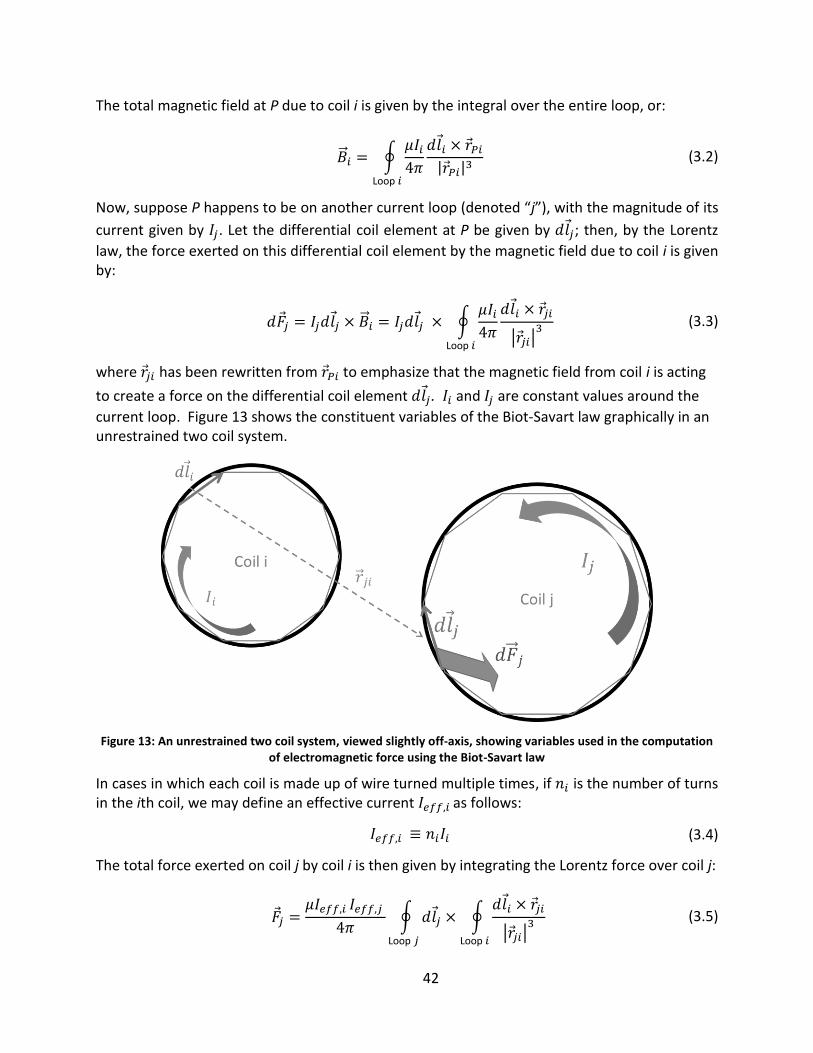
42

The total magnetic field at P due to coil i is given by the integral over the entire loop, or:

∮

| | Loop

(3.2)

Now, suppose P happens to be on another current loop (denoted “j”), with the magnitude of its

current given by . Let the differential coil element at P be given by ; then, by the Lorentz

law, the force exerted on this differential coil element by the magnetic field due to coil i is given by:

∮

| |

Loop

(3.3)

where has been rewritten from to emphasize that the magnetic field from coil i is acting

to create a force on the differential coil element . and are constant values around the

current loop. Figure 13 shows the constituent variables of the Biot-Savart law graphically in an unrestrained two coil system.

Figure 13: An unrestrained two coil system, viewed slightly off-axis, showing variables used in the computation of electromagnetic force using the Biot-Savart law

In cases in which each coil is made up of wire turned multiple times, if is the number of turns in the ith coil, we may define an effective current as follows:

(3.4)

The total force exerted on coil j by coil i is then given by integrating the Lorentz force over coil j:

∮ ∮

| |

Loop Loop

(3.5)

43

By Newton’s 2nd and 3rd laws, the force acting on coil i from coil j is given by

(3.6)

The forces act on the centers of mass of each coil, assuming that the coils are rigid. For a system with more than two coils, the force is equal to the summation of the contributions from each of the N-1 other coils (N-1 instead of N because the self-contribution of force from coil j is 0).

Since a coil responding to the magnetic fields of other coils will move and rotate, the vector variables of current element direction and position in the above equation change with time for each coil in the system. As such, the delay in the response of a given coil due to the finite propagation speed of electromagnetic waves must be taken into account. In our case, however,

so long as we are interested in time scales much greater than | | ⁄ , where c is the speed of

light (3×108 m/s), the effect of the delay will be negligible.

By denoting the position of the center of mass of the jth coil in the inertial coordinate system by an overbar, , we have:

∑

∮ ∮

| |

Loop Loop

(3.7)

Equation 3.7 allows us to solve for as a result of electromagnetic force over time.

The only closed-form analytical solution of this formula is for the calculation of the force on a single particle along the coil’s axis. For an axially symmetric coil, the magnetic field at a point P along the axis of symmetry out of the plane of the coil has the analytical solution:

| |

⁄ (3.8)

where is calculated in Tesla, R is the coil radius in meters, I is the current in amps, n is the number of turns of wire in the coil, and x is the distance in meters along the axis from the center of the coil. There is no clean analytical solution for a multi-coil problem besides Equation 3.7. Therefore, a numerical approximation of the force between the coils is required in order to study the behavior of the coils over time, accomplished by numerically performing the line integrals above. In this thesis, we investigate the dynamics of the coils using numerical models constructed in MATLAB and Simulink.

44

3.1.2 Rigid body dynamics and rotation

In addition to the translational motion of two coils in space, the moment and resultant rotation induced by asymmetric forces on differential elements across the coil must be taken into account.

By the force expressions given above, the torque exerted on the ith coil about its center of mass is given by:

∑

∮ ∮

| |

Loop Loop

(3.9)

where is the location of the differential element with respect to the global inertial

coordinate system, and is the vector from differential element to the center of the coil, providing the moment arm of the torque formulation.

As with any analysis of rigid body motion, care must be taken in how the orientation of each body (in this case, the individual coils) is parameterized. We update the center of mass of each coil using purely Newton’s second law with the cumulative force, but the orientation in space must also be defined at each timestep. In this thesis, the orientation of the coils in space is parameterized by means of a quaternion.

The use of quaternions to describe the orientation of a body in space is well established—for a full account of the theory, the reader is referred to, e.g. [26]. We describe the approach in relation to coil dynamics briefly:

We attach a coordinate system (called the body coordinate system and denoted ) to the

ith coil. is the moment of inertia matrix of the ith coil calculated with respect to its center of mass, given by:

[

]

(3.10)

We have chosen so that it is aligned with the principal axes of the coil; the third entry in

the diagonal of corresponds with the axis normal to the plane of the coil. moves

along with the coil relative to the global reference frame.

45

Torques that are induced by asymmetric electromagnetic forces (or constraining elements, to be discussed in the next section) create rotation of the coil about its center of mass and thus

also create rotation of with respect to the global reference frame. The direction cosine

matrix describes that rotation by serving as a coordinate transformation from the body

frame to the global reference frame (or vice versa, if A is transposed). The matrix ,

when multiplied to the right by the set of vectors that define the positions of the points around the coil around its center, effects the appropriate rotation upon the coil as per the torque, inertia, and initial velocity and acceleration on the coil.

The dynamical response of the coils is calculated using Newton’s 2nd law in angular form, or

(3.11)

where the angular acceleration of the body is .

We define with the help of quaternions , comprised of Euler symmetric parameters, with which can be written without the use of trigonometric functions. A quaternion encodes a rotation (the magnitude of which is the first value in the quaternion) around an axis (defined with the second, third and fourth values in the quaternion). The initial quaternion, encoding no rotation, is =[1;0;0;0]. Each time step, the quaternion is updated with the rotation resulting from the induced torque and is used to define , which is then used to update the position in the global reference frame of the coil.

3.2 Incorporation of constraining elements

The equations of motion presented above are for unconstrained coils. Ultimately, mechanical elements (possibly in conjunction with appropriate current controllers for the coils) must be employed in order to execute desired geometrical configurations of the coils in space. The coils and these constraining elements then serve as the primary structure of the deployable element. Below, we describe incorporation of hinges and tethers into the equations of motion.

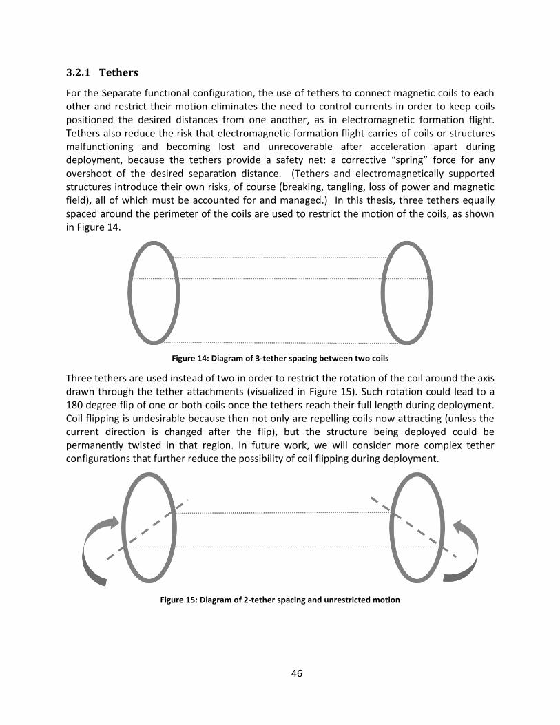
46

3.2.1 Tethers

For the Separate functional configuration, the use of tethers to connect magnetic coils to each other and restrict their motion eliminates the need to control currents in order to keep coils positioned the desired distances from one another, as in electromagnetic formation flight. Tethers also reduce the risk that electromagnetic formation flight carries of coils or structures malfunctioning and becoming lost and unrecoverable after acceleration apart during deployment, because the tethers provide a safety net: a corrective “spring” force for any overshoot of the desired separation distance. (Tethers and electromagnetically supported structures introduce their own risks, of course (breaking, tangling, loss of power and magnetic field), all of which must be accounted for and managed.) In this thesis, three tethers equally spaced around the perimeter of the coils are used to restrict the motion of the coils, as shown in Figure 14.

Figure 14: Diagram of 3-tether spacing between two coils

Three tethers are used instead of two in order to restrict the rotation of the coil around the axis drawn through the tether attachments (visualized in Figure 15). Such rotation could lead to a 180 degree flip of one or both coils once the tethers reach their full length during deployment. Coil flipping is undesirable because then not only are repelling coils now attracting (unless the current direction is changed after the flip), but the structure being deployed could be permanently twisted in that region. In future work, we will consider more complex tether configurations that further reduce the possibility of coil flipping during deployment.

Figure 15: Diagram of 2-tether spacing and unrestricted motion

47

In the Separate deployment, the coils start close to one another with tethers slack, as shown in Figure 17. Suppose the coils are aligned along their central axes, and the tethers—all identical to one another—are parallel to these axes. Once current is run through the coils in opposing directions, the coils begin to accelerate away from each other until the coils are apart, where is the unstretched length of a tether.

In order to numerically approximate the position x of each of the tethered coils, we want to solve for x in:

(3.12)

In order to determine in each time step, we use Newton’s second law:

∑

(3.13)

where ∑

is the sum of all forces working on coil i. The total force on each coil is a sum

of the forces due to the elasticity of the tethers, damping, and electromagnetic forces:

∑

∑

(3.14)

The directions of the forces comprising Equations 3.14 are shown representatively in Figure 16 with electromagnetic forces repelling two coils apart and elastic forces acting in taut or stretched tethers to pull the coils back together. A damping force works opposite the direction of coil velocity at each timestep. Note that the magnitudes/sizes of the arrows in Figure 16 are arbitrary and that the damping force is modeled as acting on the coils, though it is located on the tethers in Figure 16 for image clarity.

Figure 16: Conceptual illustration of electromagnetic, elastic tether, and damping forces in tethered deployment when tethers are taut or stretched

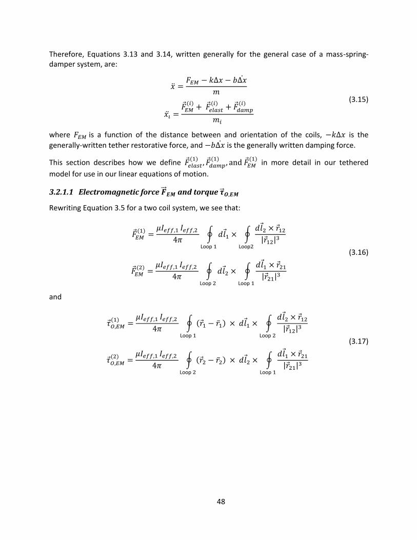
48

Therefore, Equations 3.13 and 3.14, written generally for the general case of a mass-spring-damper system, are:

(3.15)

where is a function of the distance between and orientation of the coils, is the

generally-written tether restorative force, and is the generally written damping force.

This section describes how we define

in more detail in our tethered

model for use in our linear equations of motion.

3.2.1.1 Electromagnetic force and torque

Rewriting Equation 3.5 for a two coil system, we see that:

∮ ∮

| | Loop Loop

∮ ∮

| | Loop Loop

(3.16)

and

∮ ∮

| | Loop Loop

∮ ∮

| | Loop Loop

(3.17)

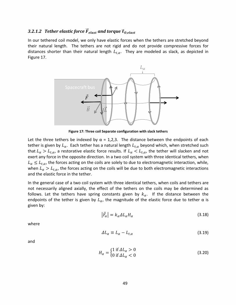
49

3.2.1.2 Tether elastic force and torque

In our tethered coil model, we only have elastic forces when the tethers are stretched beyond their natural length. The tethers are not rigid and do not provide compressive forces for distances shorter than their natural length . They are modeled as slack, as depicted in Figure 17.

Figure 17: Three coil Separate configuration with slack tethers

Let the three tethers be indexed by α = 1,2,3. The distance between the endpoints of each tether is given by . Each tether has a natural length beyond which, when stretched such that , a restorative elastic force results. If , the tether will slacken and not exert any force in the opposite direction. In a two coil system with three identical tethers, when , the forces acting on the coils are solely to due to electromagnetic interaction, while,

when , the forces acting on the coils will be due to both electromagnetic interactions and the elastic force in the tether.

In the general case of a two coil system with three identical tethers, when coils and tethers are not necessarily aligned axially, the effect of the tethers on the coils may be determined as follows. Let the tethers have spring constants given by . If the distance between the endpoints of the tether is given by , the magnitude of the elastic force due to tether α is given by:

| | (3.18)

where

(3.19)

and

{

(3.20)

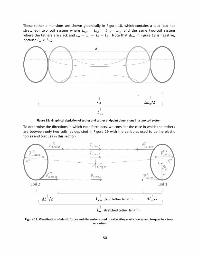
50

These tether dimensions are shown graphically in Figure 18, which contains a taut (but not stretched) two coil system where and the same two-coil system where the tethers are slack and . Note that in Figure 18 is negative, because

Figure 18: Graphical depiction of tether and tether endpoint dimensions in a two coil system

To determine the directions in which each force acts, we consider the case in which the tethers are between only two coils, as depicted in Figure 19 with the variables used to define elastic forces and torques in this section.

Figure 19: Visualization of elastic forces and dimensions used in calculating elastic forces and torques in a two-coil system

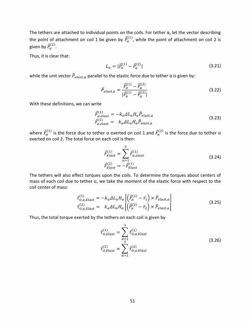
51

The tethers are attached to individual points on the coils. For tether α, let the vector describing

the point of attachment on coil 1 be given by

, while the point of attachment on coil 2 is

given by

.

Thus, it is clear that:

|

| (3.21)

while the unit vector parallel to the elastic force due to tether α is given by:

|

| (3.22)

With these definitions, we can write

(3.23)

where

is the force due to tether α exerted on coil 1 and

is the force due to tether α exerted on coil 2. The total force on each coil is then:

∑

(3.24)

The tethers will also effect torques upon the coils. To determine the torques about centers of mass of each coil due to tether α, we take the moment of the elastic force with respect to the coil center of mass:

[(

) ]

[(

) ] (3.25)

Thus, the total torque exerted by the tethers on each coil is given by

∑

∑

(3.26)

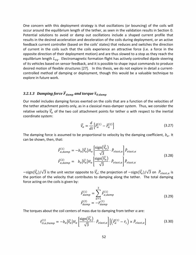
52

One concern with this deployment strategy is that oscillations (or bouncing) of the coils will occur around the equilibrium length of the tether, as seen in the validation results in Section 0. Potential solutions to avoid or damp out oscillations include a shaped current profile that results in the desired acceleration and deceleration of the coils during deployment, or an active feedback current controller (based on the coils’ states) that reduces and switches the direction of current in the coils such that the coils experience an attractive force (i.e. a force in the opposite direction of their deployment motion) and are thus slowed to a stop as they reach the equilibrium length . Electromagnetic formation flight has actively controlled dipole steering

of its vehicles based on sensor feedback, and it is possible to shape input commands to produce desired motion of flexible structures [27]. In this thesis, we do not explore in detail a current-controlled method of damping or deployment, though this would be a valuable technique to explore in future work.

3.2.1.3 Damping force and torque

Our model includes damping forces exerted on the coils that are a function of the velocities of the tether attachment points only, as in a classical mass-damper system. Thus, we consider the

relative velocity of the two coil attachment points for tether α with respect to the inertial coordinate system:

[

] (3.27)

The damping force is assumed to be proportional to velocity by the damping coefficient, . It can be shown, then, that:

| | [ ( )

√ ]

| | [ ( )

√ ]

(3.28)

√ is the unit vector opposite to ; the projection of √ on is the portion of the velocity that contributes to damping along the tether. The total damping force acting on the coils is given by:

∑

(3.29)

The torques about the coil centers of mass due to damping from tether α are:

| | [ ( )

√ ] [(

) ] (3.30)

53

| | [ ( )

√ ] [(

) ]

where the O denotes that the torques are taken with respect to the center of mass of the coil

body and is the moment arm vector from the center of the coil i to the point of tether

attachment. The total damping torques are given by:

∑

∑

(3.31)

The translational equations of motion resulting from Equations 3.16, 3.23, 3.24, 3.28 and 3.29 are thus:

∑[

]

∮ ∮

| | Loop Loop

∑[

]

∮ ∮

| | Loop Loop

(3.32)

The total torque in the tethered system is:

∑

∑

∑

∑

∑

∑

(3.33)

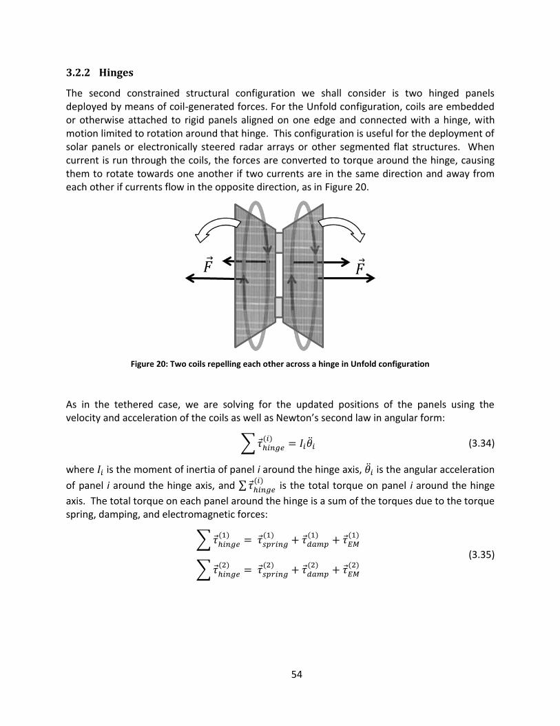
54

3.2.2 Hinges

The second constrained structural configuration we shall consider is two hinged panels deployed by means of coil-generated forces. For the Unfold configuration, coils are embedded or otherwise attached to rigid panels aligned on one edge and connected with a hinge, with motion limited to rotation around that hinge. This configuration is useful for the deployment of solar panels or electronically steered radar arrays or other segmented flat structures. When current is run through the coils, the forces are converted to torque around the hinge, causing them to rotate towards one another if two currents are in the same direction and away from each other if currents flow in the opposite direction, as in Figure 20.

Figure 20: Two coils repelling each other across a hinge in Unfold configuration

As in the tethered case, we are solving for the updated positions of the panels using the velocity and acceleration of the coils as well as Newton’s second law in angular form:

∑

(3.34)

where is the moment of inertia of panel i around the hinge axis, is the angular acceleration

of panel i around the hinge axis, and ∑

is the total torque on panel i around the hinge

axis. The total torque on each panel around the hinge is a sum of the torques due to the torque spring, damping, and electromagnetic forces:

∑

∑

(3.35)

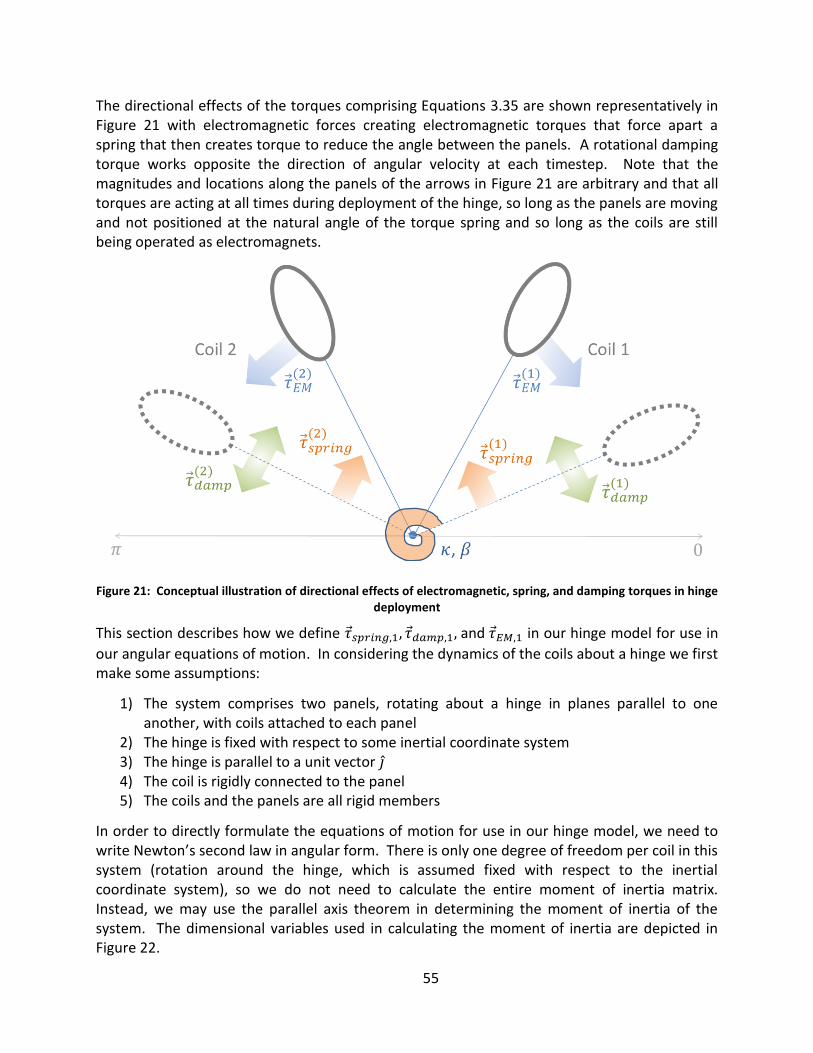
55

The directional effects of the torques comprising Equations 3.35 are shown representatively in Figure 21 with electromagnetic forces creating electromagnetic torques that force apart a spring that then creates torque to reduce the angle between the panels. A rotational damping torque works opposite the direction of angular velocity at each timestep. Note that the magnitudes and locations along the panels of the arrows in Figure 21 are arbitrary and that all torques are acting at all times during deployment of the hinge, so long as the panels are moving and not positioned at the natural angle of the torque spring and so long as the coils are still being operated as electromagnets.

Figure 21: Conceptual illustration of directional effects of electromagnetic, spring, and damping torques in hinge deployment

This section describes how we define and in our hinge model for use in

our angular equations of motion. In considering the dynamics of the coils about a hinge we first make some assumptions:

1) The system comprises two panels, rotating about a hinge in planes parallel to one another, with coils attached to each panel

2) The hinge is fixed with respect to some inertial coordinate system 3) The hinge is parallel to a unit vector 4) The coil is rigidly connected to the panel 5) The coils and the panels are all rigid members

In order to directly formulate the equations of motion for use in our hinge model, we need to write Newton’s second law in angular form. There is only one degree of freedom per coil in this system (rotation around the hinge, which is assumed fixed with respect to the inertial coordinate system), so we do not need to calculate the entire moment of inertia matrix. Instead, we may use the parallel axis theorem in determining the moment of inertia of the system. The dimensional variables used in calculating the moment of inertia are depicted in Figure 22.

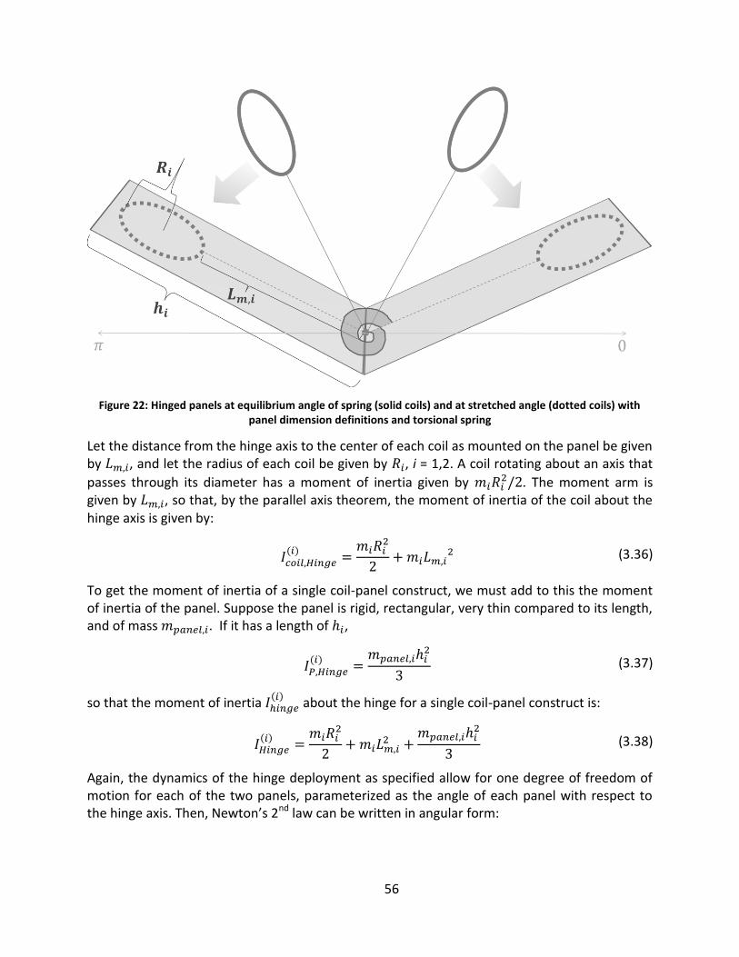
56

Figure 22: Hinged panels at equilibrium angle of spring (solid coils) and at stretched angle (dotted coils) with panel dimension definitions and torsional spring

Let the distance from the hinge axis to the center of each coil as mounted on the panel be given by , and let the radius of each coil be given by , i = 1,2. A coil rotating about an axis that

passes through its diameter has a moment of inertia given by . The moment arm is

given by , so that, by the parallel axis theorem, the moment of inertia of the coil about the hinge axis is given by:

(3.36)

To get the moment of inertia of a single coil-panel construct, we must add to this the moment of inertia of the panel. Suppose the panel is rigid, rectangular, very thin compared to its length, and of mass . If it has a length of ,

(3.37)

so that the moment of inertia about the hinge for a single coil-panel construct is:

(3.38)

Again, the dynamics of the hinge deployment as specified allow for one degree of freedom of motion for each of the two panels, parameterized as the angle of each panel with respect to the hinge axis. Then, Newton’s 2nd law can be written in angular form:

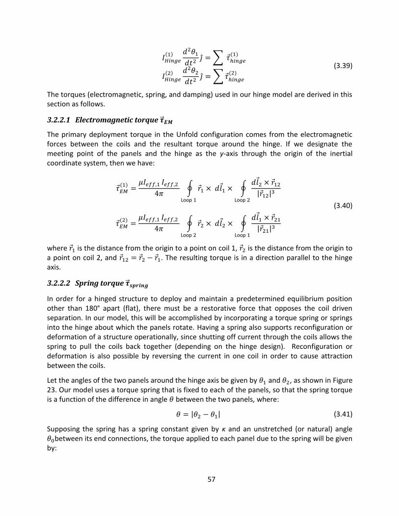
57

∑

∑

(3.39)

The torques (electromagnetic, spring, and damping) used in our hinge model are derived in this section as follows.

3.2.2.1 Electromagnetic torque

The primary deployment torque in the Unfold configuration comes from the electromagnetic forces between the coils and the resultant torque around the hinge. If we designate the meeting point of the panels and the hinge as the y-axis through the origin of the inertial coordinate system, then we have:

∮ ∮

| | Loop Loop

∮ ∮

| | Loop Loop

(3.40)

where is the distance from the origin to a point on coil 1, is the distance from the origin to a point on coil 2, and . The resulting torque is in a direction parallel to the hinge axis.

3.2.2.2 Spring torque

In order for a hinged structure to deploy and maintain a predetermined equilibrium position other than 180° apart (flat), there must be a restorative force that opposes the coil driven separation. In our model, this will be accomplished by incorporating a torque spring or springs into the hinge about which the panels rotate. Having a spring also supports reconfiguration or deformation of a structure operationally, since shutting off current through the coils allows the spring to pull the coils back together (depending on the hinge design). Reconfiguration or deformation is also possible by reversing the current in one coil in order to cause attraction between the coils.

Let the angles of the two panels around the hinge axis be given by and , as shown in Figure 23. Our model uses a torque spring that is fixed to each of the panels, so that the spring torque is a function of the difference in angle between the two panels, where:

| | (3.41)

Supposing the spring has a spring constant given by κ and an unstretched (or natural) angle between its end connections, the torque applied to each panel due to the spring will be given by:

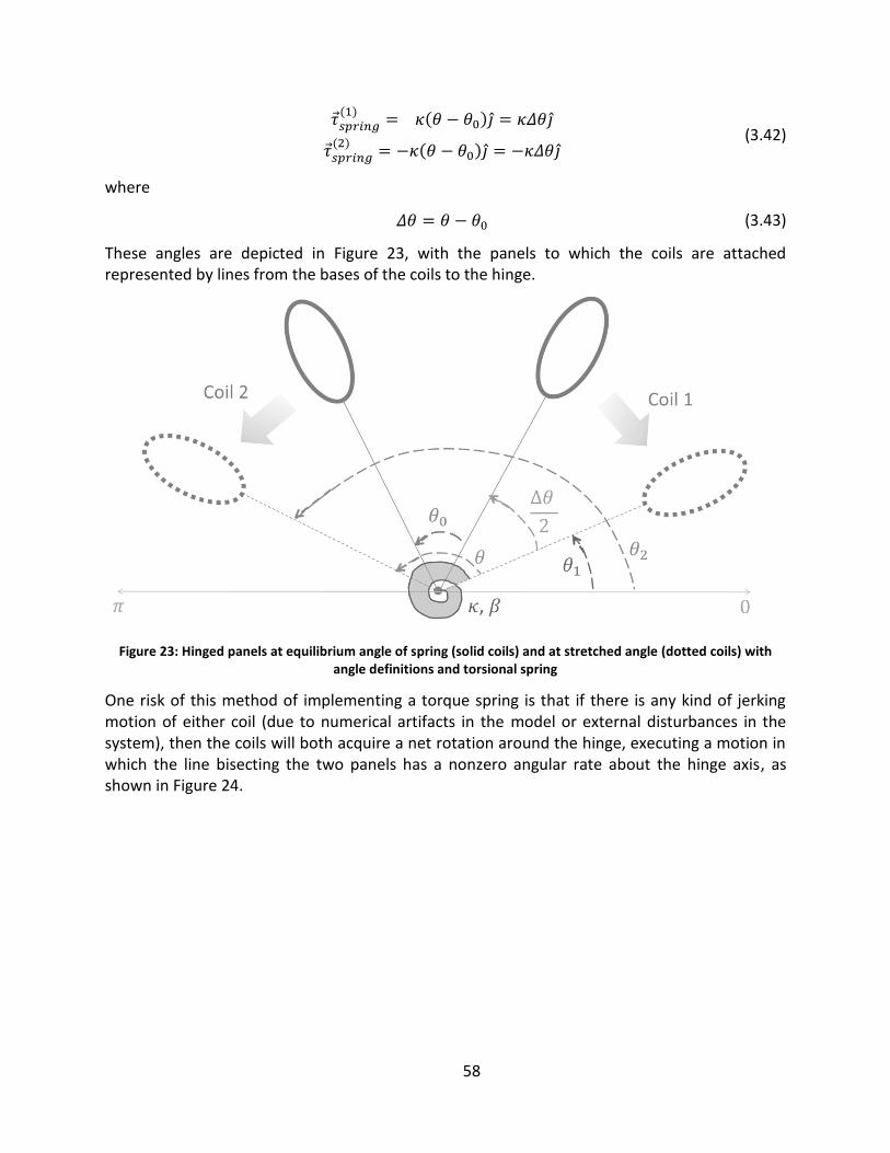
58

(3.42)

where

(3.43)

These angles are depicted in Figure 23, with the panels to which the coils are attached represented by lines from the bases of the coils to the hinge.

Figure 23: Hinged panels at equilibrium angle of spring (solid coils) and at stretched angle (dotted coils) with angle definitions and torsional spring

One risk of this method of implementing a torque spring is that if there is any kind of jerking motion of either coil (due to numerical artifacts in the model or external disturbances in the system), then the coils will both acquire a net rotation around the hinge, executing a motion in which the line bisecting the two panels has a nonzero angular rate about the hinge axis, as shown in Figure 24.

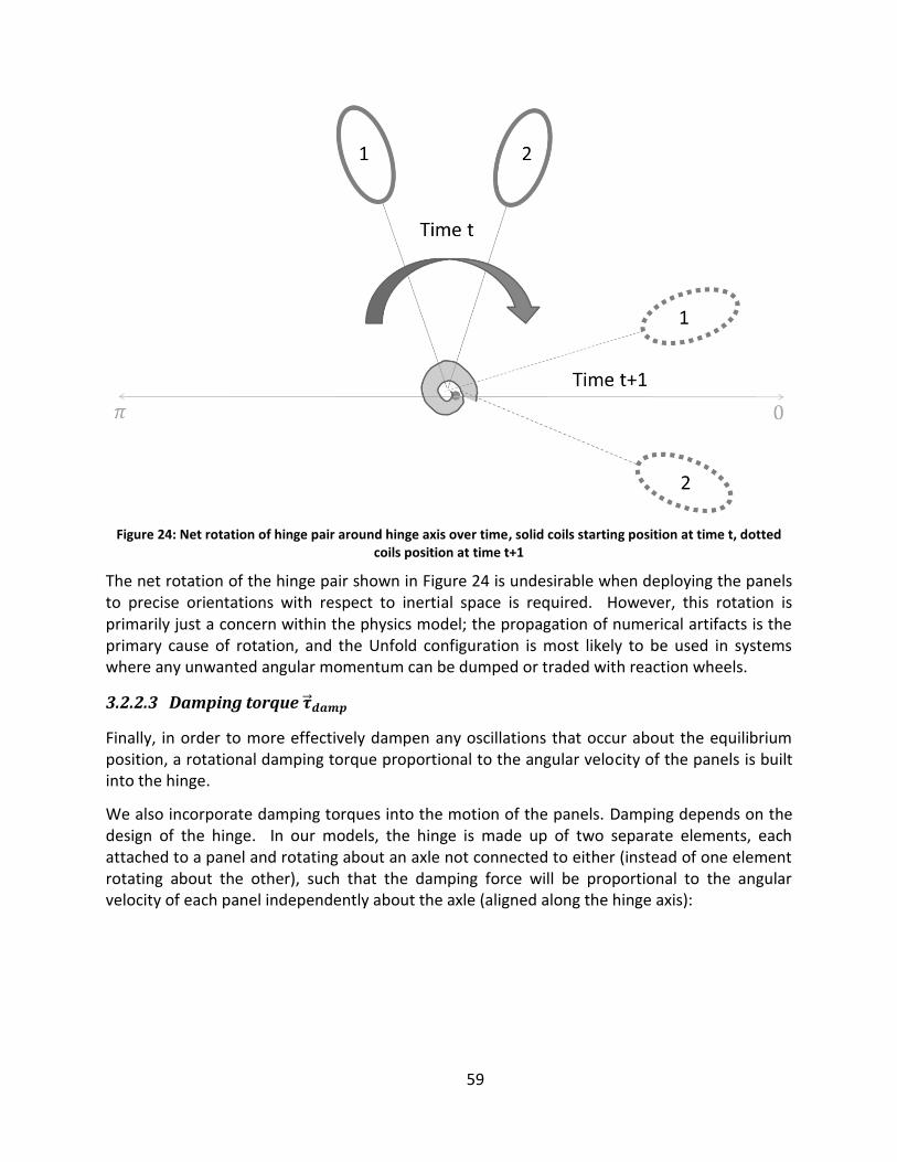
59

Figure 24: Net rotation of hinge pair around hinge axis over time, solid coils starting position at time t, dotted coils position at time t+1

The net rotation of the hinge pair shown in Figure 24 is undesirable when deploying the panels to precise orientations with respect to inertial space is required. However, this rotation is primarily just a concern within the physics model; the propagation of numerical artifacts is the primary cause of rotation, and the Unfold configuration is most likely to be used in systems where any unwanted angular momentum can be dumped or traded with reaction wheels.

3.2.2.3 Damping torque

Finally, in order to more effectively dampen any oscillations that occur about the equilibrium position, a rotational damping torque proportional to the angular velocity of the panels is built into the hinge.

We also incorporate damping torques into the motion of the panels. Damping depends on the design of the hinge. In our models, the hinge is made up of two separate elements, each attached to a panel and rotating about an axle not connected to either (instead of one element rotating about the other), such that the damping force will be proportional to the angular velocity of each panel independently about the axle (aligned along the hinge axis):

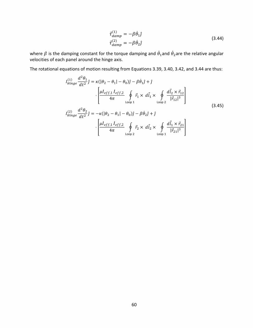
60

(3.44)

where is the damping constant for the torque damping and and are the relative angular velocities of each panel around the hinge axis.

The rotational equations of motion resulting from Equations 3.39, 3.40, 3.42, and 3.44 are thus:

| |

[

∮ ∮

| |

Loop Loop

]

| |

[

∮ ∮

| |

Loop Loop

]

(3.45)

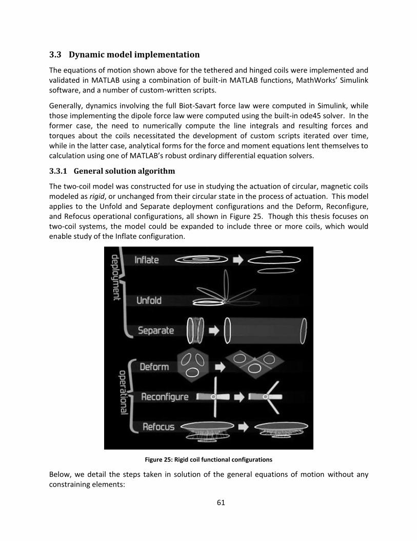
61

3.3 Dynamic model implementation

The equations of motion shown above for the tethered and hinged coils were implemented and validated in MATLAB using a combination of built-in MATLAB functions, MathWorks’ Simulink software, and a number of custom-written scripts.

Generally, dynamics involving the full Biot-Savart force law were computed in Simulink, while those implementing the dipole force law were computed using the built-in ode45 solver. In the former case, the need to numerically compute the line integrals and resulting forces and torques about the coils necessitated the development of custom scripts iterated over time, while in the latter case, analytical forms for the force and moment equations lent themselves to calculation using one of MATLAB’s robust ordinary differential equation solvers.

3.3.1 General solution algorithm

The two-coil model was constructed for use in studying the actuation of circular, magnetic coils modeled as rigid, or unchanged from their circular state in the process of actuation. This model applies to the Unfold and Separate deployment configurations and the Deform, Reconfigure, and Refocus operational configurations, all shown in Figure 25. Though this thesis focuses on two-coil systems, the model could be expanded to include three or more coils, which would enable study of the Inflate configuration.

Figure 25: Rigid coil functional configurations

Below, we detail the steps taken in solution of the general equations of motion without any constraining elements:

62

Within the model, we define the positions of φ evenly spaced points around each of two coils with respect to a global coordinate origin and assigns values for current ( ), wire

cross-sectional area, wire density per unit length ρ, radii of the coils ( ), and the moments of inertia of each ring ( ).

At each timestep, the force and torque on each coil as a result of the magnetic field of the other coil must be calculated. This is done using a double for-loop that uses Equations 3.16 and 3.17 to calculate the force and torque on each point around Coil 1 from every point on Coil 2 (and vice versa), summing the contributions on one point from Coil 2 and then summing all the resultant forces and torques around Coil 1 for a final force and torque value on the coil at that timestep. The resultant forces and torques are multiplied after the loops end by the currents and appropriate constants to complete the Biot-Savart equation and calculation of Laplace force.

o For the tethered and hinged models, elastic/spring and damping forces and torques are also included in addition to electromagnetic forces and torques, as in Equations 3.32 and 3.45.

The accelerations of the centers of mass are calculated by dividing the total force by the masses of the coils, as in Equation 3.15.

The positions of the centers of mass of the coils are updated using the position and the velocity from the previous timestep.

To determine the rotation of the coil about its center of mass, the torques (one for each coil) are projected onto the local axes of the coils. The angular velocities, quaternions and direction cosine matrices are calculated from the torques, and the orientation of the coils in space are updated accordingly.

The new location is plotted and the above process is repeated in the next time step.

The block diagrams of the Simulink models for the tethered and hinged deployment configurations are included below in Figure 26 and Figure 27.

Figure 26 shows the high level block diagram of our tether Simulink model, with blocks representing the force and torque calculations from the current positions of the coils (and other globally defined parameters like mass and current), the transformation of the torque into the body frame of each coil, the updating of the quaternion and direction cosine matrix, then the updating of the positions of the coils in space.

63

Figure 26: Tether Simulink model block diagram, shown with outputs of electromagnetic force, elastic tether force, and damping force.

Figure 27 shows the high level block diagram of our hinge Simulink model, with blocks representing the force and torque calculations from the current positions of the coils around the hinge (and other globally defined parameters), the integration of torque into velocity and change in angle using the spring constant and damping coefficient of the hinge, and the updating of the location and orientation of the coils in space.

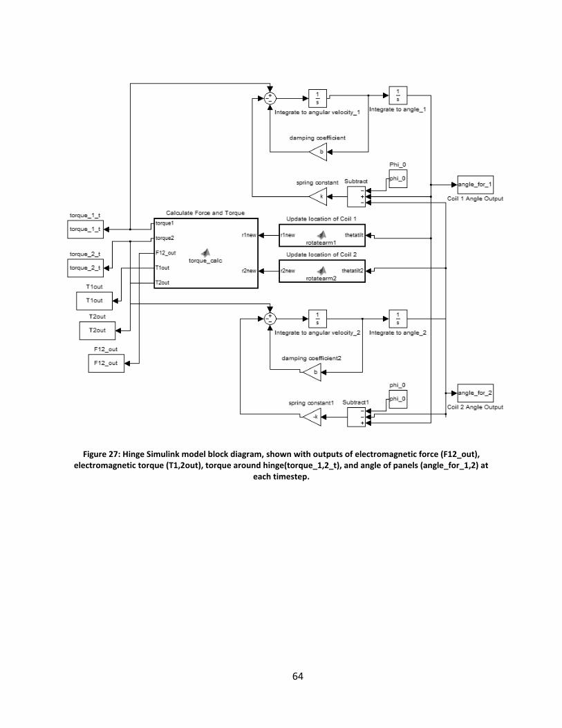
64

Figure 27: Hinge Simulink model block diagram, shown with outputs of electromagnetic force (F12_out), electromagnetic torque (T1,2out), torque around hinge(torque_1,2_t), and angle of panels (angle_for_1,2) at

each timestep.

65

3.3.2 Note on solution of stiff equations

is dependent on and the time is discretized by timesteps of varying duration in the

tether model discussed in Section 3.2.1. We see from the formula for (Equation 3.23)

that the larger k is, the larger the restorative force is for a certain . and the

electromagnetic force (Equation 3.16) act simultaneously over the course of a

timestep ; as stretches the tether, is opposing this motion. The formula for

when ≥ is very stiff when using most materials. The acting to accelerate the

coils apart over a timestep creates a that causes a that is much larger than the

for all but the smallest s (and thus the smallest s are required for these two

opposing forces to be of similar magnitudes and allow the model to converge to the approximation of continuous motion). A Simulink model utilizing the variable-timestep ode45() solver is used to select small s when ≥ and larger s when < for shorter overall run times.

66

3.4 Validation of numerical models

Validation of the numerical methods employed in solving the dynamical equations of the coils are carried out by comparing results in which the force law is governed by the Biot-Savart law with those in the dipole approximation.

Validation of the numerical approximation can be done via an approximation of the coils as magnetic dipoles at far-field distances. The far-field as discussed in this thesis is defined as the case in which the diameter D of each coil under consideration is much less than the distance between every pair of coils in the network:

| | ; (3.46)

A more thorough discussion of what constitutes this limit follows below. While validation against an exact analytic solution is not possible in the near field, we demonstrate that both the behavior of the numerical model in the near field is consistent with its behavior in the far-field, and that the behavior of the numerical model in the far-field matches that of the dipole. Thus, the validation provides confidence in the accuracy of the model.

3.4.1 Analytic dipole model

The forces exerted by two magnetic dipoles on each other are given by Schweighart [14]:

[

( )

] (3.47)

where is the vector distance between the centers of the coils, is the magnetic constant, and and are the magnetic moments of each coil, defined by:

(3.48)

being the number of turns in coil i, being the current, the area enclosed by the loop, and being the unit vector along the axis of the coil, oriented in the direction dictated by the right-hand rule following the current around the loop.

For two identical, coaxially-aligned coils with planes parallel to one another, the dipole force equation reduces to:

| | (3.49)

with the unit vector in the direction of towards the other coil. The above formula is multiplied by -1 if the currents are in opposite directions.

67

3.4.2 Sources of error in numerical approximation

There are two sources of error that contribute to the difference in force calculations between the numerical model and the far-field dipole approximation: 1) the discretization of the coils into straight line segments rather than a continuous curve, and 2) the distance between the coils. The errors resulting from these two sources decrease to zero as the number of line segments in the discretization or the distance between coils increases to infinity.

Discretization: When using the Biot-Savart force law, the number of calculations to determine the resultant force and torque on each coil due to the other’s magnetic field is O( ), with being the number of differential elements around the coil, making fine discretization of curved coils (though more accurate to the curve of the coil) computationally expensive when computing the electromagnetic force.

Distance: The numerical force falls off as ⁄ and the dipole force falls off as ⁄ , so we expect for very small ( ) values that the dipole force dominates, but then the dipole force is much greater than the numerical force right after r = 1 and then the difference between the two calculated forces goes to zero as . A quick visualization of this trend is shown in Figure 28.

Figure 28: Proportional difference between numerical and dipole approximations

There is not a specific ratio of to at which the far-field approximation becomes valid;

rather, one can determine what constitutes an acceptable percent error between the two. Figure 29 plots the initial force between a 1m diameter coil and a 0.98m diameter coil facing each other against the distance between them in both the numerical model (black) and the dipole approximation (grey), showing the convergence of the initial force values as the distance between the coils increases. The coils are slightly different sizes in order to avoid overlap of the coils in space for very small ( << 1) distances.

68

Figure 29: Comparison of numerical and dipole initial forces over a range of starting distances

Table 5 lists the error of the dipole force calculation compared to the numerical force calculation for distances that are various multiples of the coil radius.

Table 5: Error between numerical and dipole force calculations

Distance in coil radii Error (%)

1 87.4

5.021 16.5

10.05 4.7

15.07 2.2

15.98 2.0

16.98 1.8

20 1.3

69

Assuming an acceptable error in force of 2%, we find from Figure 29 and Table 5 that the distance at which the far-field approximation becomes valid is ~16 times the coil radius, or . This activity validates that the six degree-of-freedom approach presented in this chapter converges to the dipole approximation as expected at distances far from each other. There is no equivalent validation of the approach for the near-field, so this far-field convergence must suffice. We emphasize that the purpose of validation is to verify the accuracy and performance of our numerical methods in calculating the Biot-Savart force (which is a well-known consequence of the Lorentz force law and Gauss’s law and is valid at any distance between coils) and to make sure that it agrees with another valid calculation of electromagnetic force that does not require a numerical approximation to calculate, the dipole force. The fact that the dipole case only converges to the true Biot-Savart forces in the far-field does not affect the Biot-Savart formulation in the near field: if the models agree in the far-field, then the Biot-Savart formulation is closely approximating behavior in the near-field (though the discretization of the coil influences the accuracy of the behavior as well).

3.4.3 Validation models

Validation of the numerical code for coil dynamics consisted of comparing the simulation results for full dynamics (i.e. those governed by the Biot-Savart force law) with those in the dipole approximation in the appropriate distance limit. Ten different deployment configurations were used for validation purposes, five in each of 1) Axially-aligned coils with elastic tethers between them and 2) hinged coil-panel systems with torque springs attached. For axially-aligned coils, rigid body rotation is not expected to occur. Therefore, validation for the Separate configuration focused solely on the translational motion of the coils. The equations of motion implemented in the validation models will be discussed below.

3.4.3.1 Separate configuration (tethered)

For two axially aligned coils whose planes are parallel to one another, motion will exist (for either force model, dipole or numerical) in one direction. Thus, we may directly compare the axial separation of the two coils as a function of time; this will later serve to give an idea of what characteristic time scales are required deployment for various tether and coil sizes and, ultimately, for various load sizes.

The equations of motion in the Laplace force case (restated from Equation 3.32) are:

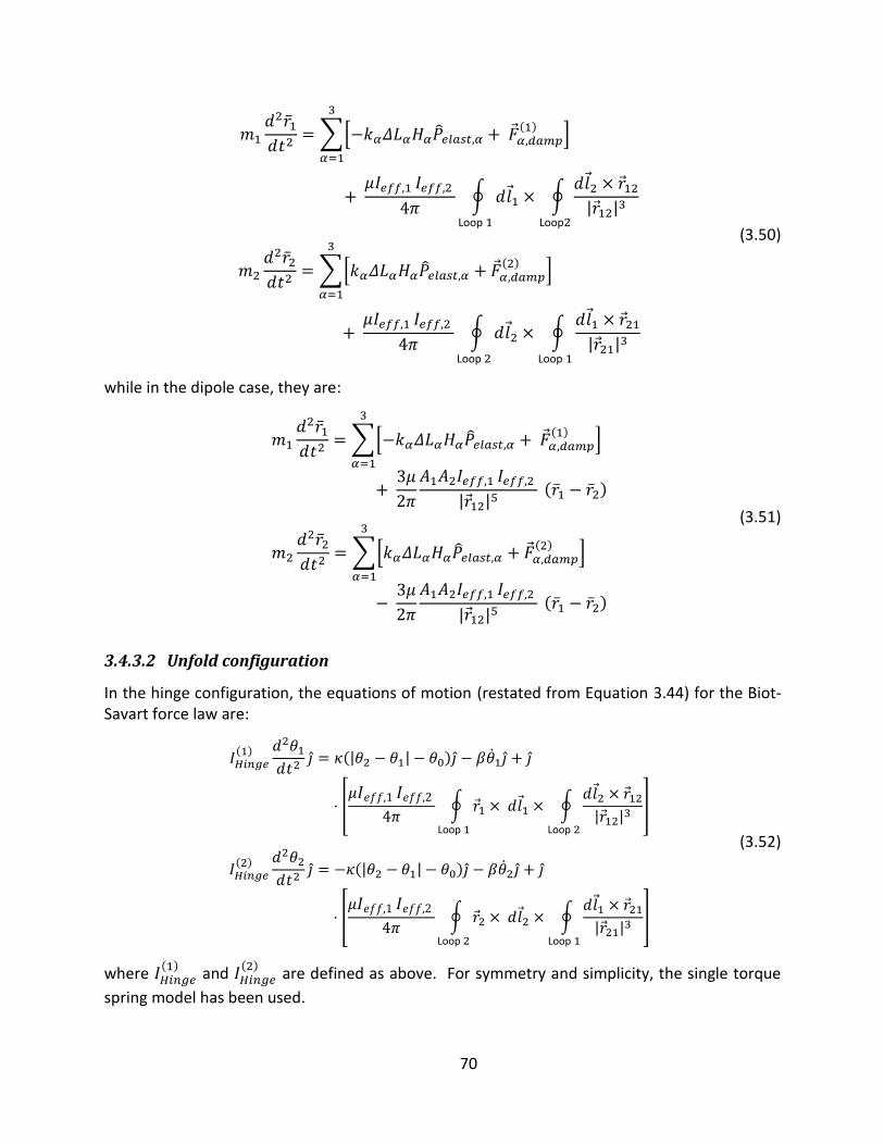
70

∑[

]

∮ ∮

| | Loop Loop

∑[

]

∮ ∮

| | Loop Loop

(3.50)

while in the dipole case, they are:

∑[

]

| |

∑[

]

| |

(3.51)

3.4.3.2 Unfold configuration

In the hinge configuration, the equations of motion (restated from Equation 3.44) for the Biot-Savart force law are:

| |

[

∮ ∮

| |

Loop Loop

]

| |

[

∮ ∮

| |

Loop Loop

]

(3.52)

where

and

are defined as above. For symmetry and simplicity, the single torque

spring model has been used.

71

For the dipole case, we consider only the situation in which each hinged panel is of the same length. Consider the expression for the force acting on the centers of each coil, again letting | | be the angle between the hinge panels, we have by the geometry:

| |

| | (3.53)

the force acting along a line that passes through the centers of the coils. If we calculate the torque due to this force about the hinge, we find (recalling that the moment arm is of length ):

(3.54)

Noting that , we have, finally:

| |

[

] (3.55)

and

[

]

(3.56)

Thus, the corresponding dipole model equations of motion are:

| |

[

]

| |

[

]

(3.57)

72

3.4.4 Validation results

The foregoing equations of motion for the Separate and Unfold configurations were solved for several variations of the physical parameters, and the dipole and numerical results compared. In the Separate case, the coils are both of radius 0.5 m. They begin, axially aligned, at a distance of 5.0 m, with the tethers having an unstretched length m. The coil wires, assumed to have the density of copper, have a cross-sectional area of:

(3.58)

have 90 turns, and current of 100 A running through them, which are typical values for industry standard HTS wire. [6] The baseline damping coefficient for a single tether is ⁄ and the baseline single tether spring constant is . The mass of a payload attached to each coil is 10 kg, which could include the weight of a cooling system for the coil or other apparatus.

In the Unfold configuration, the coils have the same radius, cross sectional area, number of turns, and current as in the Separate configuration. The baseline damping coefficient and the baseline torque spring constant is . The moment arm of the coil , while the panel has a length of and a mass of . The spring has an unstretched angle of ⁄ , and the coils

have an initial separation of ⁄ . In both cases, the coils are discretized by points; these baseline parameters are summarized in Table 6.

73

Table 6: Baseline values of physical parameters for simulation

Variables Symbol Value

General

Diameter D 1 m (=2R)

Current through wire I 100 A

# of turns n 90

Effective current

Density per unit length of wire ρ

Discretization of coil φ 17 points

Separate Configuration

Initial distance between coil centers 5 m

Unstretched length of tethers 6 m

Tether damping coefficient ⁄

Elasticity of tethers

Mass, payload 10 kg

Mass, coil

Unfold Configuration

Initial angle between coils ⁄

Unstretched angle of spring ⁄

Torque damping coefficient

Torsional spring constant

Mass of panel attached to coil 10 kg

Length of panel 20 m

Hinge moment arm length 10 m

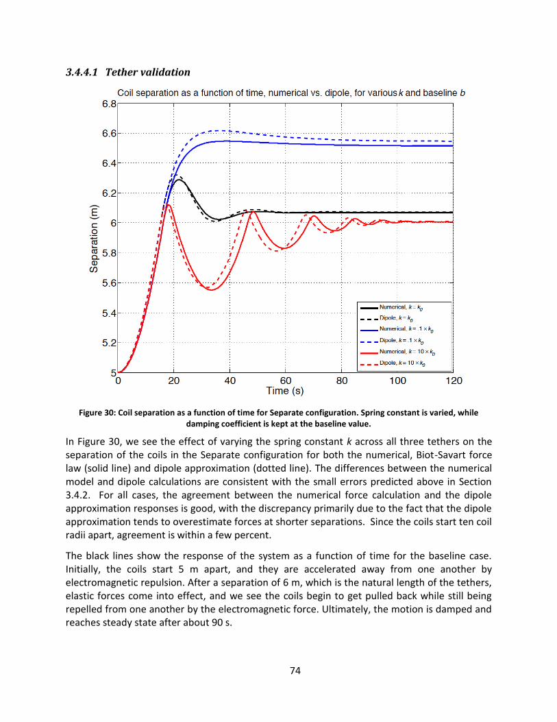
74

3.4.4.1 Tether validation

Figure 30: Coil separation as a function of time for Separate configuration. Spring constant is varied, while damping coefficient is kept at the baseline value.

In Figure 30, we see the effect of varying the spring constant k across all three tethers on the separation of the coils in the Separate configuration for both the numerical, Biot-Savart force law (solid line) and dipole approximation (dotted line). The differences between the numerical model and dipole calculations are consistent with the small errors predicted above in Section 3.4.2. For all cases, the agreement between the numerical force calculation and the dipole approximation responses is good, with the discrepancy primarily due to the fact that the dipole approximation tends to overestimate forces at shorter separations. Since the coils start ten coil radii apart, agreement is within a few percent.

The black lines show the response of the system as a function of time for the baseline case. Initially, the coils start 5 m apart, and they are accelerated away from one another by electromagnetic repulsion. After a separation of 6 m, which is the natural length of the tethers, elastic forces come into effect, and we see the coils begin to get pulled back while still being repelled from one another by the electromagnetic force. Ultimately, the motion is damped and reaches steady state after about 90 s.

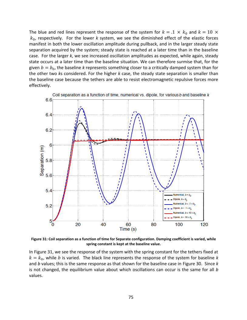
75

The blue and red lines represent the response of the system for and , respectively. For the lower k system, we see the diminished effect of the elastic forces manifest in both the lower oscillation amplitude during pullback, and in the larger steady state separation acquired by the system; steady state is reached at a later time than in the baseline case. For the larger k, we see increased oscillation amplitudes as expected, while again, steady state occurs at a later time than the baseline situation. We can therefore surmise that, for the given , the baseline k represents something closer to a critically damped system than for the other two ks considered. For the higher k case, the steady state separation is smaller than the baseline case because the tethers are able to resist electromagnetic repulsive forces more effectively.

Figure 31: Coil separation as a function of time for Separate configuration. Damping coefficient is varied, while spring constant is kept at the baseline value.

In Figure 31, we see the response of the system with the spring constant for the tethers fixed at , while is varied. The black line represents the response of the system for baseline k and b values; this is the same response as that shown for the baseline case in Figure 30. Since k is not changed, the equilibrium value about which oscillations can occur is the same for all b values.

76

We see, for diminished b ( ; blue lines), that oscillations due to elastic forces (once again, coming into play once the separation is greater than 6 m) are less effectively damped than in the baseline case. For the larger, case (red lines), we see that the system is close to being critically damped, if slightly overdamped. Nevertheless, the high b case reaches steady state slightly sooner than the baseline case. Again, qualitative agreement between the numerical and dipole cases is good.

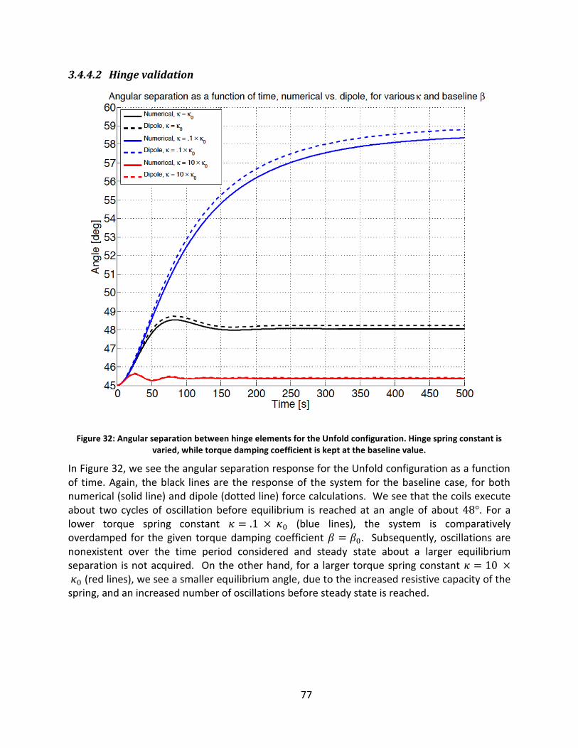
77

3.4.4.2 Hinge validation

Figure 32: Angular separation between hinge elements for the Unfold configuration. Hinge spring constant is varied, while torque damping coefficient is kept at the baseline value.

In Figure 32, we see the angular separation response for the Unfold configuration as a function of time. Again, the black lines are the response of the system for the baseline case, for both numerical (solid line) and dipole (dotted line) force calculations. We see that the coils execute about two cycles of oscillation before equilibrium is reached at an angle of about . For a lower torque spring constant (blue lines), the system is comparatively overdamped for the given torque damping coefficient . Subsequently, oscillations are nonexistent over the time period considered and steady state about a larger equilibrium separation is not acquired. On the other hand, for a larger torque spring constant (red lines), we see a smaller equilibrium angle, due to the increased resistive capacity of the spring, and an increased number of oscillations before steady state is reached.

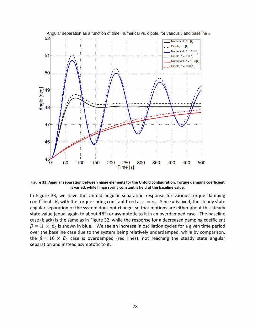
78

Figure 33: Angular separation between hinge elements for the Unfold configuration. Torque damping coefficient is varied, while hinge spring constant is held at the baseline value.

In Figure 33, we have the Unfold angular separation response for various torque damping coefficients , with the torque spring constant fixed at . Since is fixed, the steady state angular separation of the system does not change, so that motions are either about this steady state value (equal again to about ) or asymptotic to it in an overdamped case. The baseline case (black) is the same as in Figure 32, while the response for a decreased damping coefficient is shown in blue. We see an increase in oscillation cycles for a given time period over the baseline case due to the system being relatively underdamped, while by comparison, the case is overdamped (red lines), not reaching the steady state angular separation and instead asymptotic to it.

79

3.4.4.3 Effect of discretization

Figure 34: Effect of discretization on numerical calculations. Baseline tether case is calculated for Biot-Savart/numerical and dipole force laws, with the former approximated by increasingly finer discretizations .

The inset shows the same, near the oscillation peak occurring around 20 s.

In the previous sections, we investigated the response of the Separate and Unfold configurations as a function of time for both the dipole and Biot-Savart force laws. The numerical calculation of the latter depended upon the discretization of the coil, with the number of discrete points approximating the circular shape of the coil. Again, the baseline used in the previous calculations was 17. Nevertheless, it is important to understand the effect of varying from the standpoint of numerical accuracy, while for computational efficiency, it is worthwhile to keep as small as possible without sacrificing that accuracy. The choice of also has a greater impact in the near-field than in the far-field, making the selection of a representative more important for accuracy in the near-regime than in the far field as explored in Figure 34.

In Figure 34, we show the effect of varying on the response of the Separate configuration, with baseline parameters used for k and b. For reference, the dipole calculation is shown as the dotted black line. The smallest discretization considered, = 9, is shown in solid black, while the responses for = 17, 25, and 33 are shown in blue, red, and green, respectively. While the error is considerable for the = 9 case, the = 17, 25, and 33 cases are close to one another, with the = 17 and 25 approaching the = 33 line, which is naturally closest to the true

80

response. Since for each integration time step, the number of calculations goes as , we have chosen for both its relative speed and accuracy.

81

3.4.5 Note on elasticity of panel

We note that there exists an expression for the torque about the center of mass of a coil in the dipole limit. The expression is

[ (

)]

[ (

)]

(3.59)

While there will be a tendency for the magnetic moments to want to rotate about their centers due to the above torques, it is important to note that, as long as the panels are taken to be rigid, these torques exert no influence on the motion of the coil about the hinge axis. The influence of these torques would only be manifest if the panels were elastic, in which case the torques around the center of the coils would impart a moment on the panel resulting in bending of the panel. Accounting for this would necessitate solving the dynamic bending equations for the panels and would, to an extent determined by the deployment geometry and the material properties of the panel, affect the distance between the coils.

To gauge what this criterion would be for which bending is appreciable, we may conduct a simple order of magnitude analysis. From the theory of beam bending, we have that the bending moment of a beam is given by:

(3.60)

where x is a coordinate directed along the axis of the unbent beam, E is the elastic modulus of the beam material, and J (not to be confused with the current) is the area moment of inertia of the beam. If we approximate the deflection y of the beam due to the dipole torque as and take , then we have, using the dipole torque expression,

(3.61)

or, rearranging,

(3.62)

Now, the criterion for which this would have a negligible effect on the hinge dynamics of the coil-panel system (by altering the coil center-to-coil center distance) is that: 1

1 A more precise statement may be

| |

| |

; however, for simplicity, we use the given

relation.

82

(3.63)

or

(3.64)

Since E is typically on the order of Pa for metals and μ = T·m /A, we can rewrite the above in a more illuminating manner by considering a lower elastic modulus case:

(3.65)

This criterion will generally be easily satisfied. Furthermore, since at short distances, the dipole approximation for forces and torques tends to overestimate that due to the actual force law (see below), the above expression may be taken as a general rule for ensuring that bending effects are negligible.

3.4.6 Motion of a coil under its own force in Expand configuration

Consider a flexible coil that is in some noncircular configuration (as in Figure 35). If current is run through this coil, a given differential coil element will experience a force due to the electromagnetic forces exerted on it by all other elements on the coil. It is therefore possible for a stowed coil to reconfigure itself, or Expand, into a different shape under the influence of its own electromagnetic interactions. We note that, for the rigid coil considered elsewhere in this thesis, such self-interactions have no bearing on the shape of the coil, so that in that case, it is assumed that the coil can effectively “absorb” the effect of self-interactions.

Figure 35: Expand deployment configuration

Suppose we have a flexible coil, the position of a point on the coil given by . Let us parameterize the position of a point on the coil by the coil length s, so that, in general, , where t is time. If the string is of constant length (or inextensible), the equations of motion for the string are given by:

(

)

(3.66)

The second equation is a restatement of the Pythagorean theorem as applied to a infinitesimal coil element. is the magnitude of the local tension in the string, so that the vector

83

(3.67)

is a force acting across the cross section of the coil. For an inelastic coil, both equations above must be solved simultaneously. If however the coil is elastic, following a linear elastic force law, the equations of motion reduce to a generalized wave equation:

[

] (3.68)

where E is the elastic modulus of the coil material and is the cross sectional area of the coil. In general, both are a function of s, but, if the coil material is uniform along its length, we have:

(3.69)

The force is calculated from the Biot-Savart law given before, but applied to the coil itself:

| | ∫

| |

(3.70)

where is the vector to any point on the coil not equal to and is the differential coil element at . An in depth discussion of the dynamics of self-coil deployment will be reserved for future work; nevertheless, we include here some preliminary results of calculations relevant to the self-force deployment.

Figure 36: Instantaneous self force on coil for two different coil shapes. Direction and magnitude of force indicated in arbitrary units.

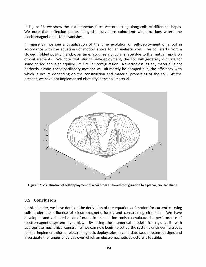
84

In Figure 36, we show the instantaneous force vectors acting along coils of different shapes. We note that inflection points along the curve are coincident with locations where the electromagnetic self-force vanishes.

In Figure 37, we see a visualization of the time evolution of self-deployment of a coil in accordance with the equations of motion above for an inelastic coil. The coil starts from a stowed, folded position, and, over time, acquires a circular shape due to the mutual repulsion of coil elements. We note that, during self-deployment, the coil will generally oscillate for some period about an equilibrium circular configuration. Nevertheless, as any material is not perfectly elastic, these oscillatory motions will ultimately be damped out, the efficiency with which is occurs depending on the construction and material properties of the coil. At the present, we have not implemented elasticity in the coil material.

Figure 37: Visualization of self-deployment of a coil from a stowed configuration to a planar, circular shape.

3.5 Conclusion

In this chapter, we have detailed the derivation of the equations of motion for current-carrying coils under the influence of electromagnetic forces and constraining elements. We have developed and validated a set of numerical simulation tools to evaluate the performance of electromagnetic system dynamics. By using the numerical models for rigid coils with appropriate mechanical constraints, we can now begin to set up the systems engineering trades for the implementation of electromagnetic deployables in candidate space system designs and investigate the ranges of values over which an electromagnetic structure is feasible.

85

4 Chapter 4 – Feasibility

In this chapter, we will study the feasibility of electromagnetic structures in space systems by using the models described in Chapter 3 to generate data over a range of design variables for the Separate and Unfold functional configurations, including current, coil diameter, number of turns, and others. These data are intended to provide a means of trading electromagnetic designs with one another for different application requirements. We will also introduce the prevailing trades between variables and between electromagnetic structures and alternative structural technologies such as inflatables and tensegrity structures.

4.1 Electromagnetic structure design variables

Electromagnetic structures have a variety of independent design variables as well as dependent design variables that are a function of the other variables. Table 7 displays several of the most important variables in the design vector for electromagnetic structures as well as their interdependencies, which are listed in the third column.

Table 7: Design variables

Variables Symbol Function of?

Independent, General

Current through wire I --

Diameter D --

# of turns n --

Density per unit length of wire ρ --

Initial distance between coil centers --

Initial angle between coils --

Angle between coils (over time) --

Stowed structure length --

Damping coefficient b, --

Discretization of coil φ --

Independent, Tethered

Unstretched length of tethers --

Elasticity of tethers k --

Independent, Hinged

Torsional spring constant κ --

Mass of panel attached to coil --

Unstretched angle of spring --

86

Dependent

Effective current I, n

Current element Idl φ, D

Mass (each coil) m D, n, ρ

Mass (total) m,

Distances from elements on coil 1 to coil 2 D, d, θ, φ

Force (one element on another) F Idl,

Force (total on coil) F

Distance between coil centers (over time) d , F, , κ, m,

Force (dipole) D, n, d, θ

Acceleration a F, m

Characteristic/Equilibrium length , d, and k (if applicable)

Size ratio S ,

Torque τ F, D

Hinge moment arm length d,

Equilibrium angle of hinge F, κ,

Deployment time T , m, b, k,

Moment of inertia ,

m, , , D,

There are several other design variables that come into play when more than two coils are being considered, the coils have variable current controllers, or when the coils are different sizes, but for now we are just examining two-coil, same-sized coil systems with constant currents throughout the deployment.

87

4.2 Reformulation of equations of motion for trade space analysis

Before exploring the variable or trade space, it is important to note that the number of independent variables, when the equations of motion are written as is, is large. To examine variance across each of the dependent variables as a function of changing each independent variable individually would be an overwhelming amount of data and plots. Therefore, it is worth exploring methods by which the dimensionality of the variable space can be reduced. One method by which this can be accomplished is via non-dimensionalization of the equations of motion. This process, which is commonly used in fluid dynamics and heat and mass transfer, greatly reduces the variable space by creating dimensionless variables that are combinations of the original ones. The process will be demonstrated below for both the Separate and Unfold configurations. We assume that in both cases the relevant geometries and properties for each coil, panel, and tether are the same (i.e. , , etc.).

First, we choose an important, characteristic geometrical variable against which we scale all variables in the problem that have dimensions of length; next, we do the same for the time scale. We choose R, the radius of each coil, as the characteristic length variable. We choose as the characteristic time variable , which we set arbitrarily to 1 second. Now, we proceed to define dimensionless auxiliary variables based on the variable originally appearing in the equations of motion; these dimensionless auxiliary variables will be distinguished by tildes “~” or asterisks “*” and are given in Table 8.

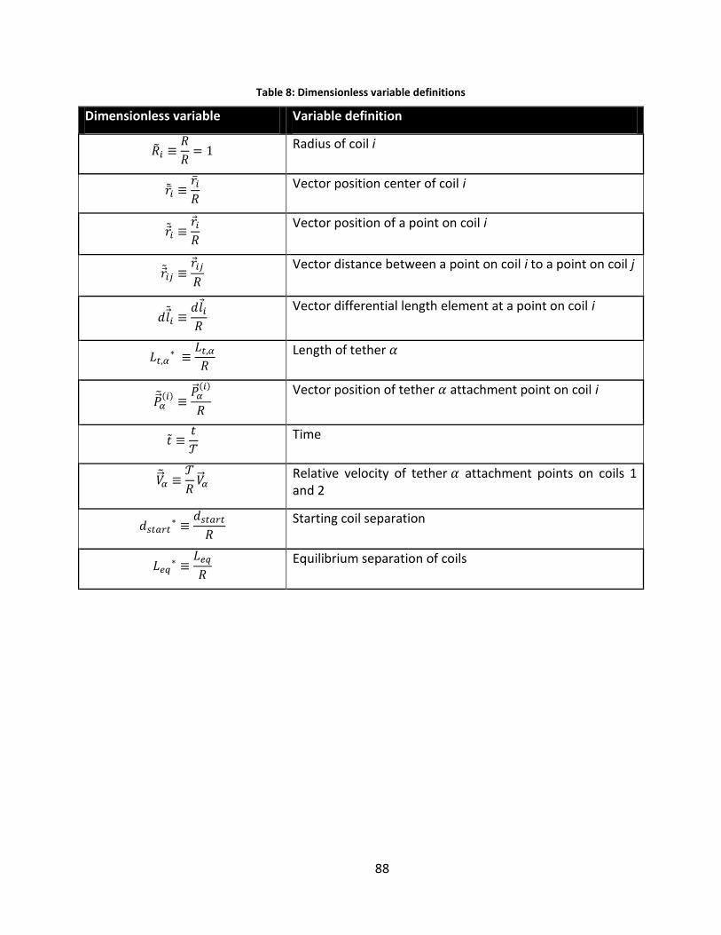
88

Table 8: Dimensionless variable definitions

Dimensionless variable Variable definition

Radius of coil i

Vector position center of coil i

Vector position of a point on coil i

Vector distance between a point on coil i to a point on coil j

Vector differential length element at a point on coil i

Length of tether

Vector position of tether attachment point on coil i

Time

Relative velocity of tether attachment points on coils 1 and 2

Starting coil separation

Equilibrium separation of coils

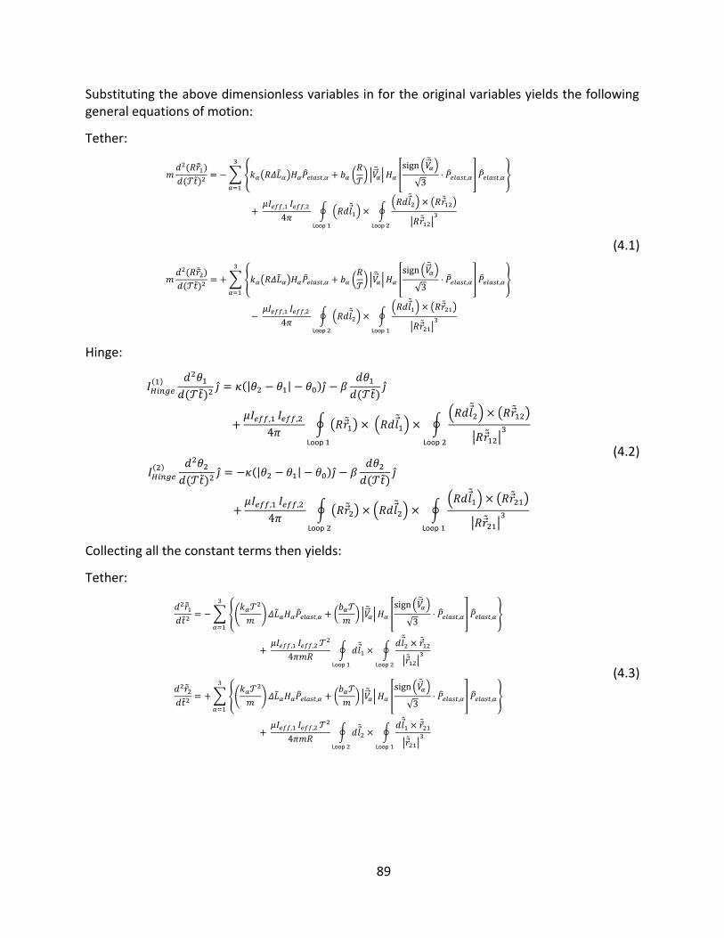
89

Substituting the above dimensionless variables in for the original variables yields the following general equations of motion:

Tether:

∑ { ( ) (

) |

| [

( )

√ ] }

∮ (

) ∮

( ) ( )

| |

Loop Loop

∑ { ( ) (

) |

| [

( )

√ ] }

∮ (

) ∮

( ) ( )

| |

Loop Loop

(4.1)

Hinge:

| |

∮ ( ) (

) ∮

( ) ( )

| |

Loop Loop

| |

∮ ( ) (

) ∮

( ) ( )

| |

Loop Loop

(4.2)

Collecting all the constant terms then yields:

Tether:

∑ {(

) (

) |

| [

( )

√ ] }

∮

∮

| |

Loop Loop

∑ {(

) (

) |

| [

( )

√ ] }

∮

∮

| |

Loop Loop

(4.3)

90

Hinge:

| |

∮

∮

| |

Loop Loop

| |

∮

∮

| |

Loop Loop

(4.4)

Next, we will redefine the dimensionless coefficients from the above equations in order to simplify the expressions. We also prescribe “baseline” values to each of the constituent variables in order to find a baseline value for each of the dimensionless parameters to use in anchoring plots of variable trades. The dimensionless quantities presented below in Table 9 now represent the key parameters for each functional configuration:

Table 9: Dimensionless parameter definitions

Dimensionless parameter

Parameter definition

Baseline values of included variables

Dimensionless parameter values for trades [Baseline]

Tether (Separate) force coefficient

10.2 kg

= 1.588

Tether (Separate) spring constant

⁄ 10.2 kg

0.010

Tether (Separate) damping constant

⁄ 10.2 kg

0.065

Hinge (Unfold) force coefficient

Hinge (Unfold) spring constant

7.443

Hinge (Unfold) damping constant

0.045

91

We are able to plot dimensionless dependent variables of interest against these dimensionless parameters in order to study the effects of certain system trades in each of the Separate and Unfold configurations as well as the behavior of unconstrained coils. Section 4.3 introduces and models several of the more interesting trades.

92

4.3 Trades

In each of the three models/functional configurations introduced in this thesis, there are a number of trades of system parameters that can be investigated in order to see relative sensitivity between variables as well as establish what combinations of parameters result in a viable system design. This section will discuss these trades from a mission level perspective and then explore them in detail using the models we have constructed.

Three of the most important parameters across most space missions are mass, required power, and system cost, reduction being desired in each of the three. As can be seen from the definition of the coefficient γ, force is proportional to the product of mass and current (power being proportional to the current through each coil as well as the number of coils in the system, which is fixed at two in this analysis). Therefore, mass and current can be traded against each other for a fixed γ, or γ can be reduced to a small value, thus minimizing both. The power of nondimensionalizing the variables in this problem is the ability to group these important parameters together such that the interior parameters can be switched around and still retain the same dimensionless parameter value and thus system behavior. A system designer can take the plots in this section and determine the desired γ or ξ for the desired behavior, as well as corresponding spring and damping constants, and then use the defined relationship to trade the interior parameters like mass and current. System cost is assumed to correlate positively with the number of turns in each coil and with the number of coils in the system, so lowering mass and current can be related to a reduction in system cost. Note that a complete cost analysis was not performed in the course of this Phase I work but is planned for future hardware development research.

Many of the plots in this section plot γ or ξ against deployment time T for various k* and b*. While deployment time is not usually a key performance parameter in the deployment of space structures, these plots are mainly for exploring reasonable ranges of values for the system parameters. Plotting against deployment time gives a nice visualization of how changing each variable affects the end result of the system, as well as lets us see easily when a certain design does not ever converge to a steady state. Also, some of the operational configurations that are possible with electromagnetic structures may be more time critical, such as a Deformation to avoid a collision or a Reconfiguration quickly in reaction to a sudden event of interest for observational spacecraft, making deployment time an important parameter in these cases.

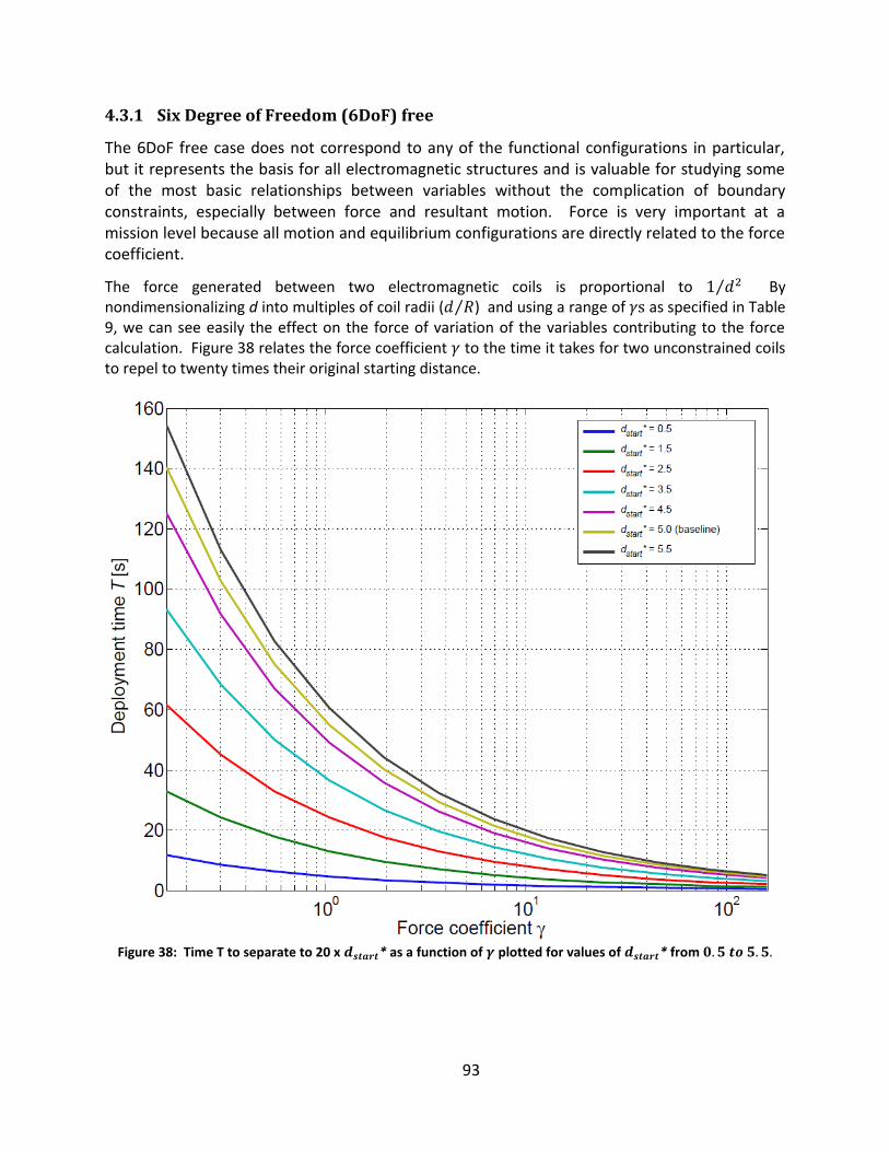
93

4.3.1 Six Degree of Freedom (6DoF) free

The 6DoF free case does not correspond to any of the functional configurations in particular, but it represents the basis for all electromagnetic structures and is valuable for studying some of the most basic relationships between variables without the complication of boundary constraints, especially between force and resultant motion. Force is very important at a mission level because all motion and equilibrium configurations are directly related to the force coefficient.

The force generated between two electromagnetic coils is proportional to ⁄ By nondimensionalizing d into multiples of coil radii ( ⁄ ) and using a range of as specified in Table 9, we can see easily the effect on the force of variation of the variables contributing to the force calculation. Figure 38 relates the force coefficient to the time it takes for two unconstrained coils to repel to twenty times their original starting distance.

Figure 38: Time T to separate to 20 x * as a function of plotted for values of * from

94

Deployment time decreases with increased force, which follows from Newton’s second law. Since force is comprised of the force coefficient and a term dependent on distance between the coils, the distance term dominates the force calculation for small s, especially for small *s, and we see that the lines are divergent and that T is influenced strongly by * for small s. High s dominate the force calculation and so we see convergence and little dependence by T on with high s.

95

4.3.2 Tethered constraints in Separate configuration

The tethered case presented in this thesis examines the behavior of axially aligned coils during separation, or the configuration pictured in Figure 14 with three tethers. The behavior of coils with altered angles (which introduces torques on the coils), axial offsets or attraction instead of repulsion will be investigated further in our Phase II work.

4.3.2.1 Force versus deployment time T

The deployment time of two tethered coils depends on the electromagnetic force between them, and the damping coefficient and spring constant of the tethers. The values of used in the plots in this chapter are for each tether; effectively, the spring constants are three times this value since there are three tethers in the system. The electromagnetic force depends on two parameters in the nondimensionalized equations of motion: and the distance | | between the coils. Deployment time in the tethered case is defined as the time the system takes to reach the steady state. For numerical calculations, we define the steady state to be the case in which both the relative velocity and acceleration of the two coils are arbitrarily close to zero:

|

| |

| (4.5)

For our calculations, we choose:

(4.6)

The following plots investigate how the deployment time T is a function of , , , *, and *. These variables encompass most of those variables from Table 7 that affect the motion and steady state position of the system without our plots becoming redundant with variables that are closely related to one another. In each of the following cases, one variable is being varied, and the others are fixed at the baseline values given in Table 9.

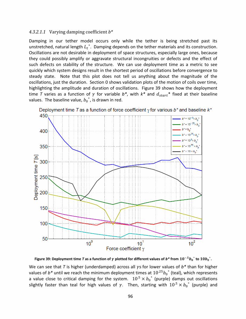
96

4.3.2.1.1 Varying damping coefficient b*

Damping in our tether model occurs only while the tether is being stretched past its unstretched, natural length

. Damping depends on the tether materials and its construction. Oscillations are not desirable in deployment of space structures, especially large ones, because they could possibly amplify or aggravate structural incongruities or defects and the effect of such defects on stability of the structure. We can use deployment time as a metric to see quickly which system designs result in the shortest period of oscillations before convergence to steady state. Note that this plot does not tell us anything about the magnitude of the oscillations, just the duration. Section 0 shows validation plots of the motion of coils over time, highlighting the amplitude and duration of oscillations. Figure 39 shows how the deployment time T varies as a function of for variable b*, with k* and * fixed at their baseline values. The baseline value,

, is drawn in red.

Figure 39: Deployment time T as a function of plotted for different values of b* from to

.

We can see that T is higher (underdamped) across all for lower values of b* than for higher values of b* until we reach the minimum deployment times at

(teal), which represents a value close to critical damping for the system.

(purple) damps out oscillations slightly faster than teal for high values of . Then, starting with

(purple) and

97

continuing on through the progressively larger values of (gold) and

(grey), we see a trend back up towards longer, overdamped Ts. The general trend is towards longer Ts from smaller s, since smaller electromagnetic forces result in smaller accelerations, and, hence, smaller damping forces and longer oscillatory motion. For the values of damping at and around the baseline (red, teal), the deployment time remains fairly consistent across the span of s (after an initial startup lag due to the small forces) because larger electromagnetic forces are met with larger damping forces in response to their higher velocity and are damped out just as quickly as medium forces in this critical damping regime.

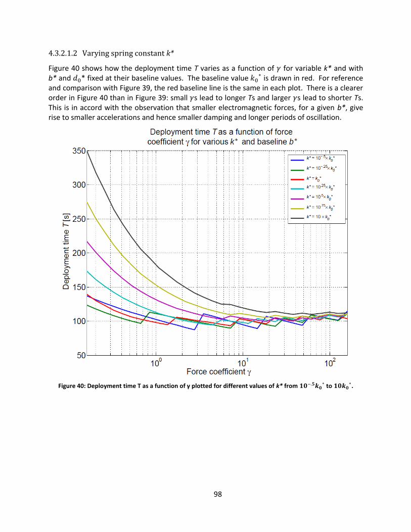
98

4.3.2.1.2 Varying spring constant k*

Figure 40 shows how the deployment time T varies as a function of for variable k* and with b* and * fixed at their baseline values. The baseline value

is drawn in red. For reference and comparison with Figure 39, the red baseline line is the same in each plot. There is a clearer order in Figure 40 than in Figure 39: small s lead to longer Ts and larger s lead to shorter Ts. This is in accord with the observation that smaller electromagnetic forces, for a given b*, give rise to smaller accelerations and hence smaller damping and longer periods of oscillation.

Figure 40: Deployment time T as a function of γ plotted for different values of k* from to

.

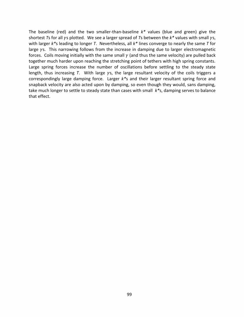
99

The baseline (red) and the two smaller-than-baseline k* values (blue and green) give the shortest Ts for all s plotted. We see a larger spread of Ts between the k* values with small s, with larger k*s leading to longer T. Nevertheless, all k* lines converge to nearly the same T for large s. This narrowing follows from the increase in damping due to larger electromagnetic forces. Coils moving initially with the same small (and thus the same velocity) are pulled back together much harder upon reaching the stretching point of tethers with high spring constants. Large spring forces increase the number of oscillations before settling to the steady state length, thus increasing T. With large s, the large resultant velocity of the coils triggers a correspondingly large damping force. Larger k*s and their larger resultant spring force and snapback velocity are also acted upon by damping, so even though they would, sans damping, take much longer to settle to steady state than cases with small k*s, damping serves to balance that effect.

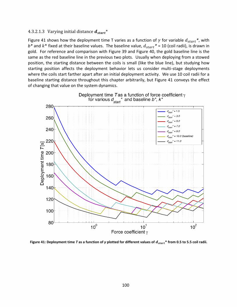
100

4.3.2.1.3 Varying initial distance *

Figure 41 shows how the deployment time T varies as a function of for variable *, with b* and * fixed at their baseline values. The baseline value, * = 10 (coil radii), is drawn in gold. For reference and comparison with Figure 39 and Figure 40, the gold baseline line is the same as the red baseline line in the previous two plots. Usually when deploying from a stowed position, the starting distance between the coils is small (like the blue line), but studying how starting position affects the deployment behavior lets us consider multi-stage deployments where the coils start farther apart after an initial deployment activity. We use 10 coil radii for a baseline starting distance throughout this chapter arbitrarily, but Figure 41 conveys the effect of changing that value on the system dynamics.

Figure 41: Deployment time T as a function of γ plotted for different values of * from 0.5 to 5.5 coil radii.

101

The behavior in Figure 41 is similar to that in Figure 40; small s lead to longer Ts, and larger s lead to shorter Ts, but the various * values converge to the same value of T at in Figure 40 while they have nowhere near converged by in Figure 41. The range of Ts for is wider in Figure 40, however. This observation means that for small , the system is more sensitive to changes in k* than in *, but for the system is almost completely insensitive to changes in k*, while it remains sensitive to changes in *. When the coils start closer to the unstretched length of the coil (in this case, * = 6 coil radii), they

have less time to accelerate before their motion is resisted by the tether spring force. That is why * = 5.5 (black) deploys the fastest regardless of ’s value; the coils do not gain a high momentum that must then be damped out to achieve equilibrium. The coils that start closer together (small *s) experience exponentially higher electromagnetic forces than those coils that start farther apart due to the force’s proportionality to the inverse of the distance between the coils squared. Larger forces result in larger oscillations that take more time to damp to steady state, so small *s have longer Ts across the board.

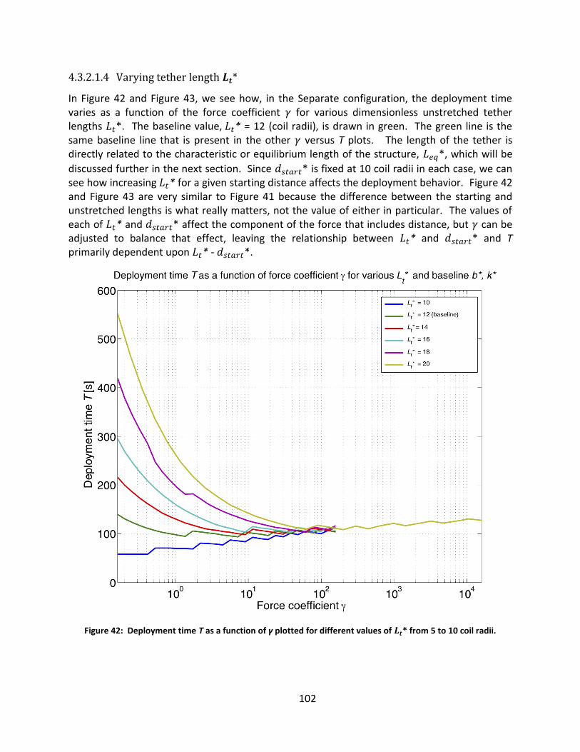
102

4.3.2.1.4 Varying tether length *

In Figure 42 and Figure 43, we see how, in the Separate configuration, the deployment time varies as a function of the force coefficient for various dimensionless unstretched tether lengths *. The baseline value, * = 12 (coil radii), is drawn in green. The green line is the same baseline line that is present in the other versus T plots. The length of the tether is directly related to the characteristic or equilibrium length of the structure, *, which will be

discussed further in the next section. Since * is fixed at 10 coil radii in each case, we can see how increasing * for a given starting distance affects the deployment behavior. Figure 42 and Figure 43 are very similar to Figure 41 because the difference between the starting and unstretched lengths is what really matters, not the value of either in particular. The values of each of * and * affect the component of the force that includes distance, but can be adjusted to balance that effect, leaving the relationship between * and * and T primarily dependent upon * - *.

Figure 42: Deployment time T as a function of γ plotted for different values of * from 5 to 10 coil radii.

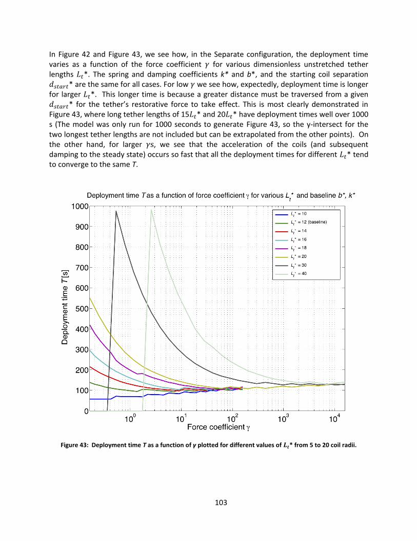
103

In Figure 42 and Figure 43, we see how, in the Separate configuration, the deployment time varies as a function of the force coefficient for various dimensionless unstretched tether lengths *. The spring and damping coefficients k* and b*, and the starting coil separation * are the same for all cases. For low we see how, expectedly, deployment time is longer for larger *. This longer time is because a greater distance must be traversed from a given * for the tether’s restorative force to take effect. This is most clearly demonstrated in Figure 43, where long tether lengths of 15 * and 20 * have deployment times well over 1000 s (The model was only run for 1000 seconds to generate Figure 43, so the y-intersect for the two longest tether lengths are not included but can be extrapolated from the other points). On the other hand, for larger , we see that the acceleration of the coils (and subsequent damping to the steady state) occurs so fast that all the deployment times for different * tend to converge to the same T.

Figure 43: Deployment time T as a function of γ plotted for different values of * from 5 to 20 coil radii.

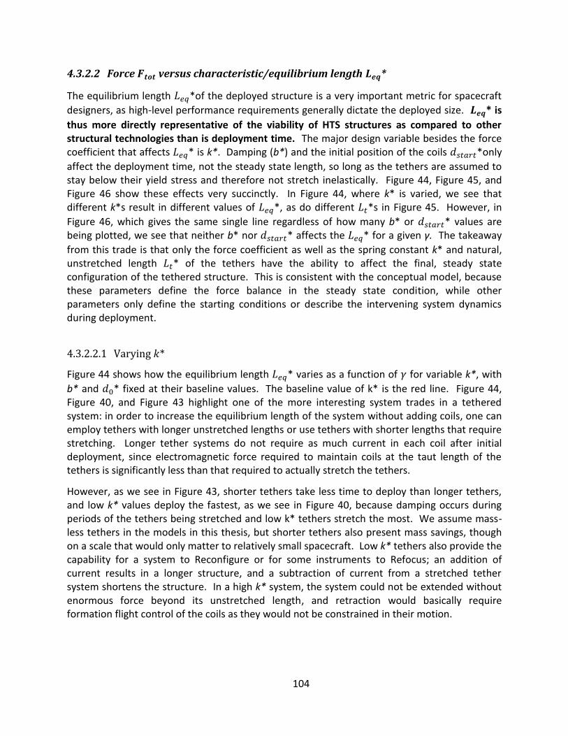
104

4.3.2.2 Force versus characteristic/equilibrium length *

The equilibrium length *of the deployed structure is a very important metric for spacecraft

designers, as high-level performance requirements generally dictate the deployed size. * is

thus more directly representative of the viability of HTS structures as compared to other structural technologies than is deployment time. The major design variable besides the force coefficient that affects * is k*. Damping (b*) and the initial position of the coils *only

affect the deployment time, not the steady state length, so long as the tethers are assumed to stay below their yield stress and therefore not stretch inelastically. Figure 44, Figure 45, and Figure 46 show these effects very succinctly. In Figure 44, where k* is varied, we see that different k*s result in different values of *, as do different *s in Figure 45. However, in

Figure 46, which gives the same single line regardless of how many b* or * values are being plotted, we see that neither b* nor * affects the * for a given γ. The takeaway

from this trade is that only the force coefficient as well as the spring constant k* and natural, unstretched length * of the tethers have the ability to affect the final, steady state configuration of the tethered structure. This is consistent with the conceptual model, because these parameters define the force balance in the steady state condition, while other parameters only define the starting conditions or describe the intervening system dynamics during deployment.

4.3.2.2.1 Varying *

Figure 44 shows how the equilibrium length * varies as a function of for variable k*, with

b* and * fixed at their baseline values. The baseline value of k* is the red line. Figure 44, Figure 40, and Figure 43 highlight one of the more interesting system trades in a tethered system: in order to increase the equilibrium length of the system without adding coils, one can employ tethers with longer unstretched lengths or use tethers with shorter lengths that require stretching. Longer tether systems do not require as much current in each coil after initial deployment, since electromagnetic force required to maintain coils at the taut length of the tethers is significantly less than that required to actually stretch the tethers.

However, as we see in Figure 43, shorter tethers take less time to deploy than longer tethers, and low k* values deploy the fastest, as we see in Figure 40, because damping occurs during periods of the tethers being stretched and low k* tethers stretch the most. We assume mass-less tethers in the models in this thesis, but shorter tethers also present mass savings, though on a scale that would only matter to relatively small spacecraft. Low k* tethers also provide the capability for a system to Reconfigure or for some instruments to Refocus; an addition of current results in a longer structure, and a subtraction of current from a stretched tether system shortens the structure. In a high k* system, the system could not be extended without enormous force beyond its unstretched length, and retraction would basically require formation flight control of the coils as they would not be constrained in their motion.

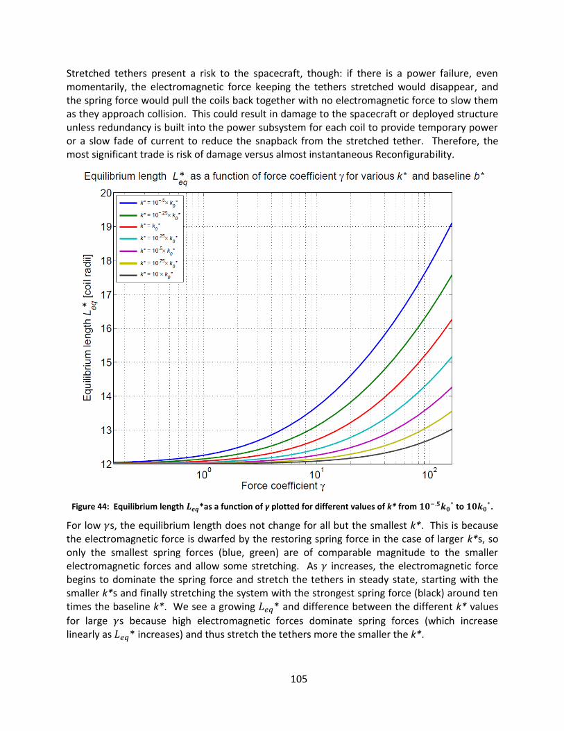
105

Stretched tethers present a risk to the spacecraft, though: if there is a power failure, even momentarily, the electromagnetic force keeping the tethers stretched would disappear, and the spring force would pull the coils back together with no electromagnetic force to slow them as they approach collision. This could result in damage to the spacecraft or deployed structure unless redundancy is built into the power subsystem for each coil to provide temporary power or a slow fade of current to reduce the snapback from the stretched tether. Therefore, the most significant trade is risk of damage versus almost instantaneous Reconfigurability.

Figure 44: Equilibrium length *as a function of γ plotted for different values of k* from to

.

For low s, the equilibrium length does not change for all but the smallest k*. This is because the electromagnetic force is dwarfed by the restoring spring force in the case of larger k*s, so only the smallest spring forces (blue, green) are of comparable magnitude to the smaller electromagnetic forces and allow some stretching. As increases, the electromagnetic force begins to dominate the spring force and stretch the tethers in steady state, starting with the smaller k*s and finally stretching the system with the strongest spring force (black) around ten times the baseline k*. We see a growing * and difference between the different k* values

for large s because high electromagnetic forces dominate spring forces (which increase linearly as * increases) and thus stretch the tethers more the smaller the k*.

*

*

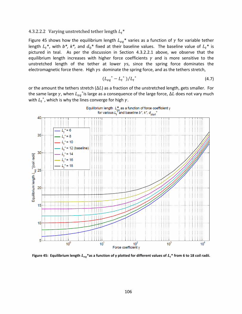
106

4.3.2.2.2 Varying unstretched tether length *

Figure 45 shows how the equilibrium length * varies as a function of for variable tether

length *, with b*, k*, and * fixed at their baseline values. The baseline value of * is pictured in teal. As per the discussion in Section 4.3.2.2.1 above, we observe that the equilibrium length increases with higher force coefficients and is more sensitive to the unstretched length of the tether at lower , since the spring force dominates the electromagnetic force there. High dominate the spring force, and as the tethers stretch,

⁄ (4.7)

or the amount the tethers stretch ( ) as a fraction of the unstretched length, gets smaller. For the same large , when

is large as a consequence of the large force, does not vary much

with , which is why the lines converge for high .

Figure 45: Equilibrium length *as a function of γ plotted for different values of * from 6 to 18 coil radii.

*

107

Varying damping coefficient b or initial distance * has zero impact on the steady state result of the system, as can be seen in Figure 46; all values of damping and initial distance settle out to the same steady state length

in the end, regardless of the time taken to do it.

The blue line in Figure 46 is the same as the baseline teal line in Figure 45.

Figure 46: Equilibrium length *as a function of γ with k* fixed at baseline * and any value of b* or *.

108

4.3.3 Hinged constraints in Unfold configuration

The hinged case presented in this thesis examines the behavior of two coils affixed to panels joined with a hinge and a torsional spring and damper along a mutual edge, or the configuration pictured in Figure 20. The following trades are intended to provide insight into the selection of design variables like panel size, effective current, spring constant, rotational damping coefficient, and natural spring angle.

4.3.3.1 Moment versus deployment time T

The deployment time of two hinged coils depends on the electromagnetic moment between them, and the damping coefficient and spring constant of the hinge. The electromagnetic force depends on two parameters in the nondimensionalized equations of motion: and the angle | | between the coils. Deployment time in the hinged case is defined as the time the system takes to reach the steady state. For numerical calculations, we define the steady state to be the case in which both the relative angular velocity and the angular acceleration of the two coils are arbitrarily close to zero:

|

| |

| (4.8)

Again, we choose:

(4.9)

The following plots investigate how the deployment time T for the Unfold configuration is a function of , , , , and . These variables encompass most of those variables from Table 7 that affect the motion and steady state angular separation of the hinged system without our plots becoming redundant with variables that are closely related to one another. In each of the following cases, one variable is being varied, and the others are fixed at the baseline values given in Table 9.

4.3.3.1.1 Varying damping

Figure 47 shows how the deployment time T varies as a function of for variable damping coefficient *, with spring constant * fixed at its baseline value. The baseline value of * is drawn in red. The longest deployment times T are for both overdamped systems (blue, black, and green lines) and underdamped systems. The shortest Ts are for those systems for which * for a given * results in close to critical damping behavior (magenta and teal lines). For the overdamped cases (black and gold), higher result in the system being forced to asymptote more quickly towards equilibrium. In the underdamped case (blue), increasing simply increases oscillations and results in the system settling to steady state after increasingly longer times. The blue line experiences ranges over where T does not increase with , followed by ranges where it does. This likely reflects a combination of several factors: an overly restrictive criterion for steady state deployment time ( ), the fact that is plotted logarithmically (as it is in all of these figures), and the relative insensitivity of the system to the moment coefficient at low values, all of which could combine and result in the presence and emphasis of numerical noise, especially for small .

109

This plot indicates to system designers that for a given *, it is possible to select an ideal, close to critically-damping * (teal and magenta) value that remains ideal regardless of s and its internal variables.

Figure 47: Deployment time T as a function of ξ plotted for different values of β* from

to .

110

4.3.3.1.2 Varying spring constant κ

Figure 48 shows how the deployment time T varies as a function of for variable spring constant *, with * fixed at its baseline value. The baseline value of * is not shown in this plot; however, the closest value is

, drawn in teal. The lowest * case plotted here (jagged blue) takes longest to reach steady state for low moment coefficients, because the system is relatively underdamped with respect to the baseline *, and, therefore, oscillations are allowed to persist for a longer period of time before reaching steady state. For low *, the system is more sensitive to various combinations of the baseline * and , resulting in the jagged nature of the line. For progressively larger *s, the deployment time is relatively insensitive to * itself but increases with and is smoother the higher *.

System designers will want to, for , choose a low * (like jagged blue) for faster deployment time; for , it is advantageous to choose a * larger than the baseline value.

Figure 48: Deployment time T as a function of ξ plotted for different values of * from to

.

111

4.3.3.1.3 Varying initial angle and natural angle

Figure 49 and Figure 50 show how the deployment time T varies as a function of for variable starting angle with * and * fixed at their baseline values. In Figure 49, the natural angle of the spring , and in Figure 50, . These two values were selected to bracket a large range of natural angles. The baseline value of both and is , drawn in this plot in teal. Starting the coils at the same angle as the natural angle of the spring (red, or ) results in the shortest deployment times for ; this is because small moments do not stretch the spring much beyond its natural length, and therefore any disturbances from this are smaller and the oscillations of lower amplitude than when For high , results in the shortest deployment times, because the spring force is already working to resist the electromagnetic repulsion at the start of deployment, so that the system can “settle” into equilibrium relatively quickly. An exception to this observation is (gold), which is so large that the spring force dominates the electromagnetic force and causes the system to oscillate too much.

Figure 49: Deployment time T as a function of ξ plotted for different values of from to and .

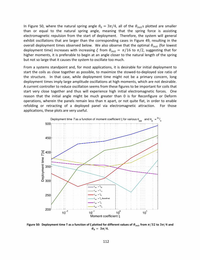
112

In Figure 50, where the natural spring angle , all of the s plotted are smaller than or equal to the natural spring angle, meaning that the spring force is assisting electromagnetic repulsion from the start of deployment. Therefore, the system will general exhibit oscillations that are larger than the corresponding cases in Figure 49, resulting in the overall deployment times observed below. We also observe that the optimal (for lowest deployment time) increases with increasing from to , suggesting that for higher moments, it is preferable to begin at an angle closer to the natural length of the spring but not so large that it causes the system to oscillate too much.

From a systems standpoint and, for most applications, it is desirable for initial deployment to start the coils as close together as possible, to maximize the stowed-to-deployed size ratio of the structure. In that case, while deployment time might not be a primary concern, long deployment times imply large amplitude oscillations at high moments, which are not desirable. A current controller to reduce oscillation seems from these figures to be important for coils that start very close together and thus will experience high initial electromagnetic forces. One reason that the initial angle might be much greater than 0 is for Reconfigure or Deform operations, wherein the panels remain less than π apart, or not quite flat, in order to enable refolding or retracting of a deployed panel via electromagnetic attraction. For those applications, these plots are very useful.

Figure 50: Deployment time T as a function of ξ plotted for different values of from to and .

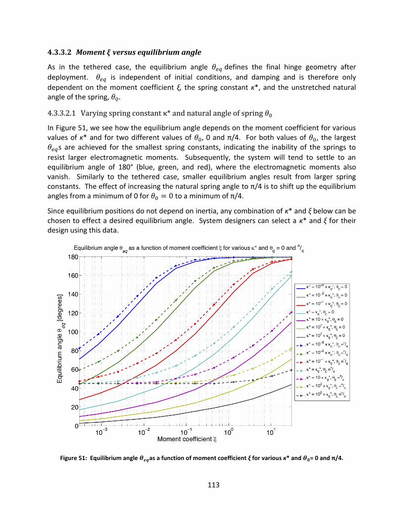
113

4.3.3.2 Moment versus equilibrium angle

As in the tethered case, the equilibrium angle defines the final hinge geometry after

deployment. is independent of initial conditions, and damping and is therefore only

dependent on the moment coefficient ξ, the spring constant κ*, and the unstretched natural angle of the spring,

4.3.3.2.1 Varying spr ng constant κ* and natural angle o spr ng

In Figure 51, we see how the equilibrium angle depends on the moment coefficient for various values of κ* and for two different values of 0 and π/4. For both values of , the largest s are achieved for the smallest spring constants, indicating the inability of the springs to

resist larger electromagnetic moments. Subsequently, the system will tend to settle to an equilibrium angle of 180° (blue, green, and red), where the electromagnetic moments also vanish. Similarly to the tethered case, smaller equilibrium angles result from larger spring constants. The effect of increasing the natural spring angle to π/4 is to shift up the equilibrium angles from a minimum of 0 for to a minimum of π/4.

Since equilibrium positions do not depend on inertia, any combination of κ* and ξ below can be chosen to effect a desired equilibrium angle. System designers can select a κ* and ξ for their design using this data.

Figure 51: Equilibrium angle as a function of moment coefficient ξ for various κ* and = 0 and π/4.

114

4.4 Conclusion

In this chapter, we have made use of the models originally presented in Chapter 3 in order to perform high-level analysis of the interconnectivity of the system variables. This analysis was enabled by introducing a number of dimensionless parameters which combine many of the design variables and facilitate systems-level analysis by reducing the dimensionality of the variable space. We focused on two primary metrics: deployment time T, and the equilibrium or characteristic length (or angle ) of the system after deployment. The effect of varying

design variables and their dimensionless counterparts was presented in such a way as to facilitate the decision-making process of a system designer.

115

5 Chapter 5: Viability

Revisiting the initial questions of the study, we see that Chapter 4 addressed Question 1, the technical feasibility question:

Question 1: Can we use electromagnetic forces generated by and acting between high-temperature superconductor current-carrying coils to move, unfold, and support parts of a spacecraft from its stowed position?

by exploring the underlying physical concepts of electromagnetic structures and the effect of system parameters on deployment dynamics and steady-state positions. From Chapter 4, we conclude that the baseline physical principles of HTS structures are sound and that limitations on the use of the technology will come from mission requirements and available subsystem budgets. Questions 2 and 3 both involve the mission and economic viability of HTS structures in the space acquisition environment:

Question 2: For which operations does this technology represent an improvement over existing or in-development options?

Question 3: What new mission capabilities does this technology enable?

and will thus be included in this chapter on the viability of HTS structures as a structural technology for space systems. A summary of the general advantages and disadvantages of HTS structures as compared to “traditional” structural options (panels, beams, motors, pyrotechnic bolts) at subsystem levels is included below in Table 10. Red text indicates a disadvantage, or area where HTS structures are competitively weaker than traditional structures and mechanisms. Green text indicates an ability or property that HTS structures have that traditional structures do not. Black indicates a parameter that depends on the properties of the electromagnetic structure design.

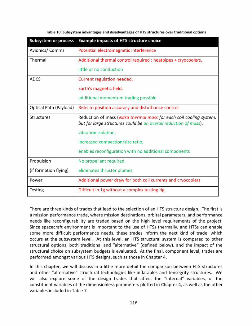
116

Table 10: Subsystem advantages and disadvantages of HTS structures over traditional options

Subsystem or process Example impacts of HTS structure choice

Avionics/ Comms Potential electromagnetic interference

Thermal Additional thermal control required : heatpipes + cryocoolers,

little or no conduction

ADCS Current regulation needed,

Earth’s magnetic field,

additional momentum trading possible

Optical Path (Payload) Risks to position accuracy and disturbance control

Structures Reduction of mass (extra thermal mass for each coil cooling system, but for large structures could be an overall reduction of mass),

vibration isolation,

increased compaction/size ratio,

enables reconfiguration with no additional components

Propulsion

(if formation flying)

No propellant required,

eliminates thruster plumes

Power Additional power draw for both coil currents and cryocoolers

Testing Difficult in 1g without a complex testing rig

There are three kinds of trades that lead to the selection of an HTS structure design. The first is a mission performance trade, where mission destinations, orbital parameters, and performance needs like reconfigurability are traded based on the high level requirements of the project. Since spacecraft environment is important to the use of HTSs thermally, and HTSs can enable some more difficult performance needs, these trades inform the next kind of trade, which occurs at the subsystem level. At this level, an HTS structural system is compared to other structural options, both traditional and “alternative” (defined below), and the impact of the structural choice on subsystem budgets is evaluated. At the final, component level, trades are performed amongst various HTS designs, such as those in Chapter 4.

In this chapter, we will discuss in a little more detail the comparison between HTS structures and other “alternative” structural technologies like inflatables and tensegrity structures. We will also explore some of the design trades that affect the “internal” variables, or the constituent variables of the dimensionless parameters plotted in Chapter 4, as well as the other variables included in Table 7.

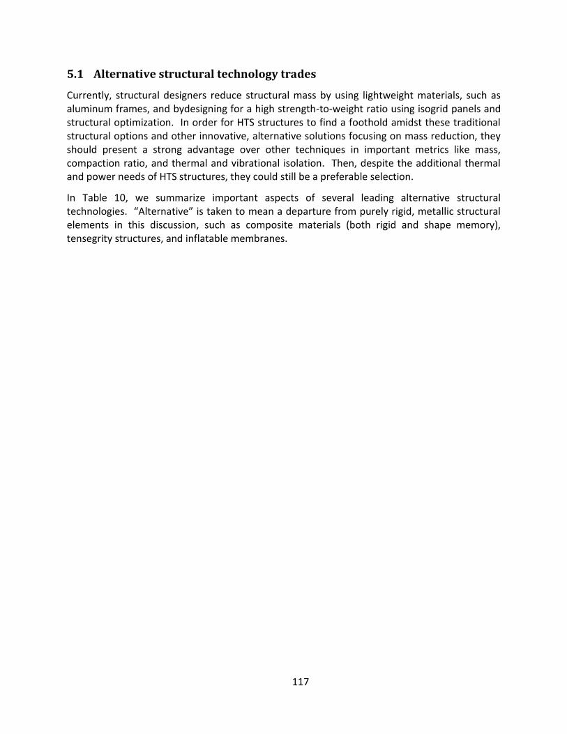
117

5.1 Alternative structural technology trades

Currently, structural designers reduce structural mass by using lightweight materials, such as aluminum frames, and bydesigning for a high strength-to-weight ratio using isogrid panels and structural optimization. In order for HTS structures to find a foothold amidst these traditional structural options and other innovative, alternative solutions focusing on mass reduction, they should present a strong advantage over other techniques in important metrics like mass, compaction ratio, and thermal and vibrational isolation. Then, despite the additional thermal and power needs of HTS structures, they could still be a preferable selection.

In Table 10, we summarize important aspects of several leading alternative structural technologies. “Alternative” is taken to mean a departure from purely rigid, metallic structural elements in this discussion, such as composite materials (both rigid and shape memory), tensegrity structures, and inflatable membranes.

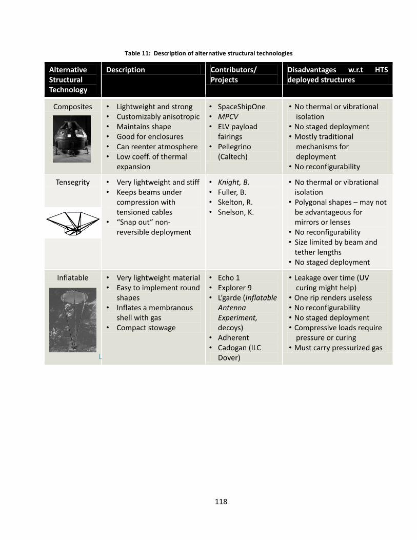
118

Table 11: Description of alternative structural technologies

Alternative Structural Technology

Description Contributors/ Projects

Disadvantages w.r.t HTS deployed structures

Composites • Lightweight and strong

• Customizably anisotropic

• Maintains shape

• Good for enclosures • Can reenter atmosphere

• Low coeff. of thermal expansion

• SpaceShipOne

• MPCV

• ELV payload fairings

• Pellegrino (Caltech)

• No thermal or vibrational isolation

• No staged deployment • Mostly traditional

mechanisms for deployment

• No reconfigurability

Tensegrity • Very lightweight and stiff • Keeps beams under

compression with tensioned cables

• “Snap out” non-reversible deployment

• Knight, B. • Fuller, B. • Skelton, R. • Snelson, K.

• No thermal or vibrational isolation

• Polygonal shapes – may not be advantageous for mirrors or lenses

• No reconfigurability

• Size limited by beam and tether lengths

• No staged deployment

Inflatable • Very lightweight material • Easy to implement round

shapes • Inflates a membranous

shell with gas • Compact stowage

• Echo 1

• Explorer 9

• L’garde (Inflatable Antenna Experiment, decoys)

• Adherent • Cadogan (ILC

Dover)

• Leakage over time (UV curing might help)

• One rip renders useless • No reconfigurability

• No staged deployment • Compressive loads require

pressure or curing

• Must carry pressurized gas

L’garde

Knight

MPCV

119

5.1.1 Comparison of HTS structures to alternative structural technologies

Table 12 qualitatively lists key trades between HTS structures and other structural support and actuation technologies. The Other Technology column lists the technology against which HTS structures are being compared. The second and third columns show the desirable attributes of the Other Technology versus HTS Structures respectively.

Table 12: Comparison of HTS structures to alternative structural technologies

Other Technology Other Tech Attribute vs. HTS Structures Attribute

Inflatables Low power and potentially lower mass

Longer lifetime

Tensegrity Low power and no thermal control

Controllability of deployment and potential reversibility

Composites Low power and no thermal control

Shape change and compaction/size ratio

Pyrotechnics Reliable impulse Deployment control and potential reversibility

Piezoelectrics Precision Range of motion

Spring-loaded booms and hinges

Lower power and potentially lower mass

Controllability of deployment and potential reversal

Traditional motorized actuators

Heritage Low mass and thermal/vibrational isolation

Table 13 depicts a qualitative comparison of electromagnetic support and the three structural support technologies listed above (inflatables, tensegrity structures, and composites) across a variety of characteristics of interest for spacecraft designers. Values of these characteristics (in this table, yes, no, or other) that are generally considered good for the specific metric by spacecraft designers are green, values that are dependent on the specifics of the implementation of the technology and could be either good or not are yellow, and those values that are considered less desirable are red. All characteristics are treated equally in this table, but in some applications, some attributes may be valued more highly than others. The takeaway from Table 13 is that HTS structures compare favorably to other structural techniques in most performance metrics associated with spacecraft structures, but that the HTS power and thermal requirements are significantly less desirable. Further development of HTS structures should focus on mitigating the risk that the power and thermal metrics present to successful technology integration.

120

Table 13: Qualitative comparison of deployable structure options

Another option is the combination of electromagnetics with other structural technologies in an attempt to combine their benefits and negate their weaknesses. For instance, other options besides simple cable tethers attached at each end to a coil exist for the Separate deployment. Thin, rigid members with joints that lock open as the coils move apart in order to guarantee a fixed distance between the coils and reduce oscillations during deployment are also a possibility, though such constraints would be more massive than tethers and serve as vibration pathways. The Separate coil configuration as modeled here is both a deployment and a support device; with rigid, locking members, it becomes purely a deployment device and thus loses the novelty of being able to perform two functions simultaneously. Another option, one that allows for Reconfiguration over the lifetime of the spacecraft, is tethers that can be reeled out from a spool or back in to change the unstretched length

121

5.2 Internal variable trades

The variables internal to the nondimensionalized coefficients used in Chapters 3 and 4 encompass other variables in the design vector for an HTS structure, including mass (of coils m, of attached components like , or of the total system ), power draw (of each coil,

taken as or of the thermal subsystem, taken as ), number of turns in the coil n, diameter of coil D, stowed structure length , the damping coefficient b or , the spring

constant k or , the temperature that a coil is maintained at , the magnetic field , and the different forces and torques.

Table 14 displays several of these system trades: the first column names an increase or decrease in one variable, and the second column reflects the reactions of other system variables to that change. Red text is a change that is generally not in the direction expressed in an objective vector for spacecraft (an example general one shown below), such as an increase in mass or power. Green text is a change that is in the direction specified in the objective vector, such as a minimization of mass or power. Black text labels variables that can optionally be changed along with the first column change and which might be good or bad or neither. In the case of increasing dimensionless spring or damping constants, for example, selection of either of these variables is likely not due to maximizing or minimizing these variables individually but rather through the maximization or minimization of another variable related to both constants from the plotted relationships in Chapter 4, such as equilibrium length.

Some of the desired maximizations and minimizations in space missions in general are listed below in an example objective vector. These objectives can be used to trade and select designs for further study. Table 14 reflects how certain system trades affect the extent to which these objectives are realized.

122

Table 14: System variable trades

Trade Effects on other variables Variables involved

Diagram

Temperature of coil ↓ in order to increase critical current density

↑ Thermal power draw ↑ ↑ Magnetic field to mass ratio ↑ ↑ Coil power draw ↑

, ,

, , m

Number of turns n in coil ↑ to increase effective current

↑ Magnetic field from higher effective current ↑ ↑ Mass of coil ↑ ↓ Current through each wire ↓ Power/mass ratio

, , , n,

Radius of coil R ↓ to increase magnetic force

↓ Mass of coil ↓ ↑ Magnetic field ↑ ↑ Force ↑ Dimensionless damping Dimensionless spring constant

R, ,

, F, k or , b or

# of coils N ↑ to reduce current in coils or increase characteristic length

↑ Mass of system↑ ↑ Thermal power draw ↑ and

[‐ Linear structural density ‐↑ Characteristic length ↑

↑ Coil power draw ↑]

or

[↑ Linear structural density ↑

‐ Characteristic length‐↓ Coil power draw ↓

]

, ,

,

123

Amount of current I ↑

↑ Coil power draw ↑ ↑ Magnetic field ↑ ↑ Force ↑ ↑ Characteristic length ↑ ↓ Size ratio ↓ Dimensionless damping Dimensionless spring constant

, ,

, F, k or , b or

Some more detailed discussion of the trades in Table 14 is included below:

Temperature of coil ↓ o This trade makes reference to the relationship between the critical current density

that an HTS wire can support and its temperature. As temperature decreases below , the critical current density in the wire also increases, so at colder temperatures, more current can be run through the same coil, and thus a higher magnetic field and force can be generated at the cost of more thermal power (to cool the coil to a lower temperature) and more coil power (to generate the higher current)

Number of turns in coil n ↑ o Increasing the number of turns in the coil increases the effective current in the coil to

and therefore increases , increasing the magnetic force. However, when current is flowing through multiple turns of a coil, the magnetic field of one turn exerts a magnetic force on the current in another turn, forcing it towards one side of the wire and effectively reducing the size channel through which the current can flow. The wire’s critical current density limits how much current can flow through any portion of the wire’s cross section, so once that limit is reached, the total current cannot increase; therefore, additional turns of wire reduce and result in a loss term.

The same change in power per unit mass value can result from an increase in mass, with power being held constant, or from a decrease in power, with the mass being held constant. The latter would indicate a decrease in effective current unless n is being increased and R is being decreased to result in the same mass but a higher possible effective current, as observable in the relationship:

where V is the voltage across the coil and is assumed constant.

124

Radius of coil R ↓ o We recall that the mass of the coil may be written:

is the linear density of the coil, given by:

and is the volume density of the coil material, n the number of turns in the coil, and the cross sectional area of the coil. We may then rewrite the dimensionless

force parameter as follows:

Hence, we see that:

so that decreasing the radius of the coil increases the magnetic force.

While it may seem like making R arbitrarily small is beneficial due to the increase in

the magnetic field through , we must keep in mind that changing R also has an effect on the dimensionless damping and spring coefficients, b* and k*, respectively:

Thus, if the designer has a limited choice of actual materials, and hence b and k, in order to implement a desired dynamical and structural configuration, R cannot be made arbitrarily large or small and must in fact be chosen so that the interplay of damping and elastic forces give the desired deployment dynamics and equilibrium configuration as per the analysis in Chapter 4.

# of coils N ↑ o The number of coils in the system N can be increased for one of two primary

purposes: the increasing of the characteristic length of the structure with the same current per coil, or the reduction of current through each coil with the same characteristic length. The first purpose results in no increase in the linear structural density, or mass per unit length, whereas the second purpose increases the linear structural density as there are now more coils for the same characteristic length. This dual choice is reflected in the bracketed terms in Table 14. Either choice results in an increase in the mass of the system and in the power required for cooling of the coils.

125

Amount of current I ↑ o For a current density below the critical value for the wire, increases in current result

in an increase in the magnetic field and thus electromagnetic force. For a given damping and spring constant, the characteristic length or angle will then increase as a result of the increased electromagnetic force. Thus, the size ratio (stowed-to-deployed) of the system will decrease but the coil power draw will increase due to the increased current.

Now that we have set up the basic constraints on coil motion, in future work we can now expand on these constraints to include multi-operation deployments, complex tether configurations and multi-hinge cases that enable Reconfiguration or temporary Deformation of a paneled structure. These studies, to occur in the course of future work, will examine the feasibility of “new mission capabilities” as motivated by Question 3.

126

5.3 Future work

The work presented in this thesis will be expanded upon considerably in our planned future work, which is the subject of a two-year NIAC Phase II study commencing with the conclusion of the NIAC Phase I effort that included much of the analysis in this thesis. The Phase II effort will expand upon the primary questions introduced in this thesis, develop MAGESTIC further towards the attainment of TRL 3, and reduce the risks associated with new technology development. Future work will include the development and testing of a flexible cryogenic heatpipe or heatshield as a key enabling technology for a number of HTS structural applications that require a flexible HTS coil (such as those in the Expand configuration). We will also perform technology trade studies and integration feasibility assessment and analysis for HTS structures in a large, complex, and fairing-limited precision structure such as JWST.

We have identified a number of potential barriers to the feasibility of HTSs as a replacement for traditional structures. We have sorted them into three categories of feasibility barriers to be addressed in Phase II in order of decreasing impact: Power and Thermal, Dynamics and Control, and Implementation. The four impact categories with which each concern is associated: Cost (dollars, mass and power), Spacecraft Performance, Development Time, and Key Enabling Technologies. The three key enabling technologies that our technology development effort focuses on are rigid deploying HTS coils, flexible deploying HTS coils, and flexible cooling systems. All of these key technologies require future experimental, modeling, and feasibility work.

The power and thermal subsystems are those most adversely affected by the use of HTSs, as described earlier in this thesis. Because a large portion of the power required by HTS structures is consumed by thermal equipment, these two subsystems are inextricably linked in our study of feasibility issues. The power and thermal barriers we will discuss in this section are:

Cost: Complex power and thermal control, generation and management,

Cost: Thermal vacuum chamber testing expenses

Performance: Power for HTS operations needing to be taken from other subsystems

Key technology: Low-power rigid heatpipes and flexible cooling systems

Performance: Lower power cryocoolers

Coil dynamics and control with coil boundary constraints, though, introduce performance feasibility issues that must be addressed in order for any technology advancement to take place and include:

Performance: Coil dynamics

Performance: Stability of configuration

Performance: Position accuracy and knowledge

Performance: Disturbances (Cryocooler vibration, solar pressure)

127

Implementation feasibility concerns center around the competitiveness of HTS structures with other technologies, either in cost, key performance metrics, or the ability of less complex HTS structures to be competitive enough of a structural option to find purchase on missions in order to gain flight heritage to then motivate the research and development of more complex HTS structures.

Cost: Cost may be uncompetitive with other structural options

Performance: Performance may be uncompetitive in multi-subsystem tradespace

Performance: Potential EMI, negatively affecting other subsystems on board or vice versa

Development Time: Technology roadmap may be too linear to allow missions to use less complex HTS structures as flight hardware prior to completion

Two more years to study the implementation of HTS structures under a NIAC Phase II allows us to:

Reduce risk in areas of uncertainty with regard to feasibility issues above

Assess the mission-general and mission-specific (JWST) impact of many of the feasibility issues discussed in this section with simulation and experimentation

Collaborate with NASA to fully understand the needs of the customer in order to lay out a reasonable and accomplishable roadmap towards integration

Advance key technologies necessary for full utilization of HTS structural configurations

Explore the impact of HTS structures on other spacecraft subsystems in greater detail, elaborating on the trades suggested in Phase I with quantitative comparisons

128

5.4 Summary and conclusions

In this thesis, we have conducted an initial feasibility study for the use of high-temperature superconducting coils as deployment and support elements in spacecraft structures. We have also introduced system performance trades that will be further quantified in the Phase II work.

In Chapter 1, we introduced the notion of high-temperature superconductors and the ways they could potentially be useful in spacecraft structures. We discussed the five primary benefits that HTS structures can offer to the aerospace community:

1. Reduced mass 2. Larger structures with same launch vehicles 3. Vibration- and thermally-isolated structures 4. Staged deployment, in-space assembly with fewer operations, and partial system

replacements 5. Reconfiguration of structures after deployment

and introduced the three primary research questions relevant to this study.

In Chapter 2, we motivated the work of Chapter 3 by discussing the physical principles underlying superconductivity and how electromagnetic interactions between conducting coils can result in their motion. We also discussed previous work in the use of electromagnetic forces for relative motion, positioning and deployment as well as the state of the industry for superconducting wire construction.

In Chapter 3, we developed the equations of motion for coils responding to electromagnetic forces while under the influence of constraining elements (i.e. tethers and hinged panels) and validated numerical models of these equations against known analytical solutions.

In Chapter 4, we modified our equations of motion for trade analysis by nondimensionalizing them and introducing several dimensionless parameters that encode many of our design variables. We presented the results of numerous simulations using the numerical models introduced in Chapter 3, detailing the response of tethered and hinged coil systems for various dimensionless parameters and, hence, combinations of the original design variables.

In Chapter 5, we discussed on the basis of the results from Chapter 4 the viability of HTS structures in the context of trade analyses. Trades were described at the mission level, the structural subsystem level, and the component level.

On the basis of the work presented in this thesis, we have come to the following conclusions:

1) The fundamental physics support the basic concept of using electromagnets for deployment.

2) With existing technology and capabilities, the use of HTS coils for the deployment activities investigated herein is achievable, though with significant work to be done in dynamic controllability, system optimization, sizing and scaling, thermal control, and mission integration analysis. Our Phase II work will address many of these topics as well as economic viability.

129

Primary goals in the near future include the completion and testing of an experimental flexible thermal system for cooling flexible HTS coils, a technology integration case study of JWST, laboratory experimental demonstrations of HTS coils unfolding panels and separating while superconducting, and models calibrated both by experiments and analytical solutions. These are the first steps along the HTS technology demonstration path, and those steps combined with the foundation laid in this thesis and the feasibility and implementation analysis to be conducted in the near future will bolster the credibility and prepare the technology for further TRL advancement.

130

Works Cited

1] D. A. Bearden, "When is a Satellite Mission Too Fast and Too Cheap?," in MAPLD International Conference, 2001.

2] J. R. Wertz, Space Mission Engineering: The New SMAD, Microcosm Press, 2011.

3] http://www.lhc-closer.es, "Superconductivity in Short," [Online]. Available: http://www.lhc-closer.es/php/index.php?i=1&s=4&p=8&e=0. [Accessed 21 May 2012].

4] Bruker Daltonics, "Record current with powder-in-tube superconductor," 2008.

5] V. Selvamanickam, "Coated Conductors: From R&D to Manufacturing to Commercial Applications," in Superconductivity Centennial Conference, Den Haag, the Netherlands, 2011.

6] SuperPower Inc., "SuperPower®2G HTS Wire Specifications," [Online]. Available: http://www.superpower-inc.com/system/files/SP_2G+Wire+Spec+Sheet_for+web_2012FEC_v2_0.pdf.

7] "HTS Cable and weave closeup," General Cable Superconductors Ltd, 2009. [Online]. Available: http://www.gcsuperconductors.com/about-us/galleries/gcsgallery/hts-cable-and-weave-closeup.

8] J. Llambes and D. Hazelton, "Advantages of Second-Generation High Temperature Superconductors for Pulsed Power Applications," in Pulsed Power Conference, Washington, DC, 2009.

9] A. Kurs, M. Soljacic and P. Fisher, "Wireless Power Transfer via Strongly Coupled Magnetic Resonances," Science, vol. 317, pp. 83-86, 2007.

10] R. Sedwick, Resonant Inductive Near-field Generation System (RINGS), DARPA Proposal BAA-10-44, University of Maryland Space Power and Propulsion Lab, 2010.

11] D. Kwon, Electromagnetic Formation Flight of Satellite Arrays, Massachusetts Institute of Technology, 2005.

12] D. Kwon and R. Sedwick, Cryogenic Heat Pipe for Cooling High Temperature Superconductors with Application to Electromagnetic Formation Flight Satellites, Massachusetts Institute of Technology, 2009.

13] E. Kong, Spacecraft Formation Flight Exploiting Potential Fields, Massachusetts Institute of Technology, 2002.

131

14] S. Schweighart, Electromagnetic Formation Flight Dipole Solution Planning, Cambridge: Massachusetts Institute of Technology, 2005.

15] A. Sakaguchi, Micro-Electromagnetic Formation Flight of Satellite Systems, Massachusetts Institute of Technology, 2007.

16] L. L. Jones, W. R. Wilson, J. Gorsuch, J. Shoer and M. Peck, "Flight Validation of a Multi-Degree-of-Freedom Flux-Pinned Spacecraft Model," in AIAA Guidance, Navigation, and Control Conference, Portland, 2011.

17] R. Zubrin, "NIAC Study of the Magnetic Sail," NASA, 1999.

18] J. Powell, G. Maise, J. Paniagua and J. Rather, "Magnetically Inflated Cable (MIC) System for Large Scale Space Structures," NASA Institute of Advanced Concepts, 2006.

19] G. Benford, O. Goronostavea, A. Prichard, J. Benford, L. Nakodym, D. Vaughan and H. Harris, "Sail deployment by microwave beam—experiments and simulations," in Space Technology And Applications International Forum, Albuquerque, 2002.

20] N. Pedreiro, "Spacecraft architecture for disturbance-free payload". Patent 6454215, 24 September 2002.

21] M. Shao, S. Turyshev, N. Pedreiro, D. Tenerreli, A. Carrier and S. Doravari, New Sciencecraft and Test Mass Concepts for the LISA Mission, 2011.

22] L. M. Elias, Dynamics of Multi-Body Space Interferometers Including Reaction Wheel Gyroscopic Stiffening Effects: Structurally Connected and Electromagnetic Formation Flying Architectures, MIT, 2004.

23] K. Amboss and W. Knauer, "Lightweight Reflecting Structures Utilizing Magnetic Deployment Forces". United States of America Patent 3605107, 17 July 1969.

24] R. Sedwick and D. Kwon, Cryogenic Heat Pipe for Cooling High Temperature Superconductors with Application to Electromagnetic Formation Flight Satellites, Massachusetts Institute of Technology, 2009.

25] Sunpower Corporation, "Sunpower Inc. - The CryoTel Family of Cryocoolers," [Online]. Available: http://www.sunpower.com/cryocoolers/cryotel.php. [Accessed 25 May 2012].

26] J. R. Wertz, Spacecraft Attitude Determination and Control, D. Reidel, 1980.

27] W. Singhose, "Command Generation for Flexible Systems," Massachusetts Institute of Technology, 1997.

132

28] D. W. Hazelton, F. Roy and P. Brownsey, "Superpower Inc. Recent Developments in 2G HTS Coil," in 2011 EUCAS (European Conference on Applied Superconductivity), Den Haag, The Netherlands, 2011.

29] Sunpower Corporation, "CryoTel Cryocooler FAQs," [Online]. Available: http://www.sunpower.com/cryocoolers/faq.php.

30] R. Sedwick, Subproposal to MIT on NASA NIAC Phase II Proposal, College Park, 2012.

High-Temperature Superconductors as Electromagnetic...

Documents

Transcript of High-Temperature Superconductors as Electromagnetic...