Identification of Trailing-Edge-Noise at

Buffet Flows Using High-Speed PIV and

Preparation of Pipe Flow Through a 90

Degree Bend PIV Investigation

ME 491: Independent Study

Charles Ferriera

July 27, 2012

1

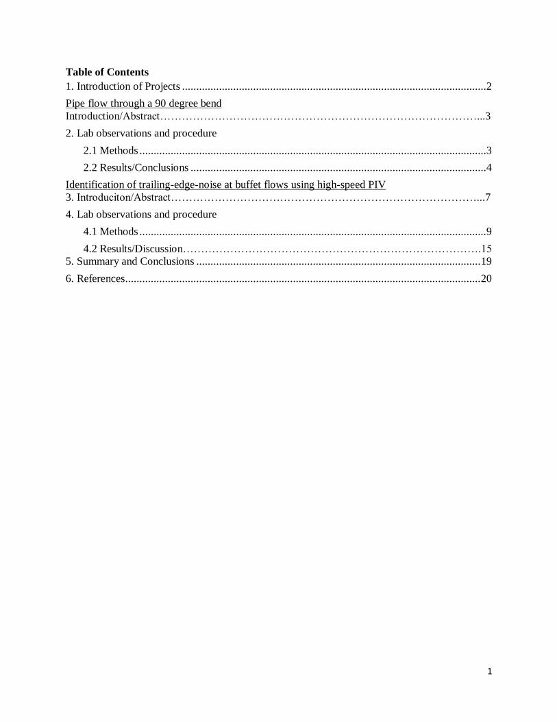
Table of Contents

1. Introduction of Projects ...........................................................................................................2

Pipe flow through a 90 degree bend

Introduction/Abstract……………………………………………………………………………...3

2. Lab observations and procedure

2.1 Methods ..........................................................................................................................3

2.2 Results/Conclusions ........................................................................................................4

Identification of trailing-edge-noise at buffet flows using high-speed PIV

3. Introduciton/Abstract…………………………………………………………………………...7

4. Lab observations and procedure

4.1 Methods ..........................................................................................................................9

4.2 Results/Discussion……………………………………………………………………….15

5. Summary and Conclusions .................................................................................................... 19

6. References............................................................................................................................. 20

2

Introduction of Projects

The projects for this independent study were both created and executed at RWTH Aachen

University under the supervision of Axel Hartmann and Franka Schröder. Both supervisors had

unique projects in which both myself and Evan McCune participated in. Schröder’s project was

focused on the fluid flow through a 90 degree pipe and Hartmann’s project was focused on

locating the cause of trailing-edge-noise at buffet flow using high-speed PIV. I chose to focus on

Hartmann's project for the majority of my time at RWTH. First, a brief summary of Particle Image

Velocimetry (PIV) will be given followed by a summary of my learning experience and

contributions to the inspection of fluid flow through a 90 degree pipe. Then my primary project

(Identification of Trailing-Edge-Noise at Buffet Flows Using High-Speed PIV) with Axel will be

discussed in detail.

Particle Image Velocimetry

The experimental procedure used to conduct the two projects was Particle Image Velocimetry

(PIV), which is a method of flow measurement that gives the user the ability to measure the

velocity field of a fluid flow. The primary equipment used in the experimental setup generally

consists of lasers, cameras, a fluid flow, and tracer particles. The fluid flow is measured by

pulsing 2 sheets of laser light in fast intervals, which illuminates tiny tracer particles within the

fluid flow. Fast cameras are used to photograph the flow exposed to the laser pulses. The cameras

are calibrated using a calibration grid of a known measurement interval in order to find the

displacement between particles captured at separate times. Since the laser pulse delay is known,

it is therefore possible to find the particle velocities. The images are analyzed via PIV computer

software using methods of cross correlation to find a distinct magnitude and direction of the fluid

flow.

Some different methods of PIV include holographic, volume tomographic, high-speed time

resolved, micro and multi-plane stereoscopic. The methods of PIV used for the experiments were

mono, high-speed time resolved and stereoscopic. Mono PIV captures images of a fluid flow

using a single camera. High speed time resolved PIV involves using high-speed lasers and

fastcams to illuminate particles and capture images of highly unsteady fluid flows. Stereoscopic

PIV consists of a laser, 2 cameras at equivalent oblique angles relative to a laser sheet and a seeded

fluid flow. This method is based off of the same principle as the human eyes, which is why it is

given the name “Stereo PIV.” An important advantage of Stereo PIV is its ability to capture all 3

velocity vector components.

3

Pipe flow through a 90 degree bend

Introduction /Abstract

In order to use computer simulations of fluid flow through a 90 degree bent pipe, validation of the

fluid flow's characteristics must be accomplished. A mono PIV setup with a single camera and

two lasers were used to capture images of the fluid flow. The lasers created a light sheet, which

illuminated tracer particles while the camera captured images of the incoming flow. The

incoming flow generally displayed dual vortices known as Dean Vortices. Using VidPIV

computer software, it was possible to analyze the images and find the magnitude and direction of

the fluid flow.

Methods

Before gathering data, it was necessary to establish a reference image so that a Matlab program

could accurately count the number of particles contained within the image. This was done via

Cam Wave computer software and trial and error, where both the grey scale and particle density

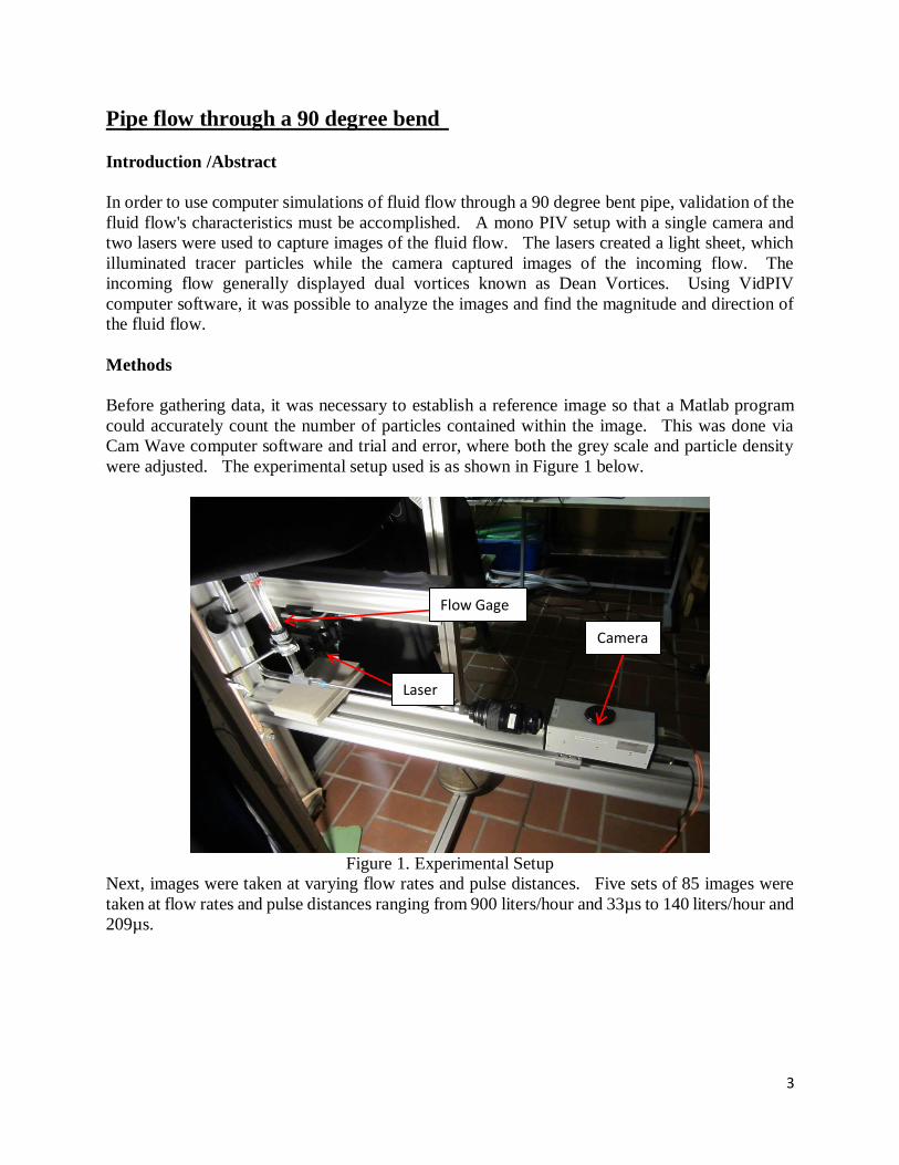
were adjusted. The experimental setup used is as shown in Figure 1 below.

Figure 1. Experimental Setup

Next, images were taken at varying flow rates and pulse distances. Five sets of 85 images were

taken at flow rates and pulse distances ranging from 900 liters/hour and 33µs to 140 liters/hour and

209µs.

Camera

Flow Gage

Laser

4

General Procedure

1. Turn on lasers 1 and 2

2. Turn on synchronizer

3. Add seeding

4. Record 85 images via Cam Wave

5. Stop recording

6. Save and Repeat 1-5 at a new flow rate and pulse width

The images were then processed by Evan McCune using VidPIV computer software.

Results/Conclusions

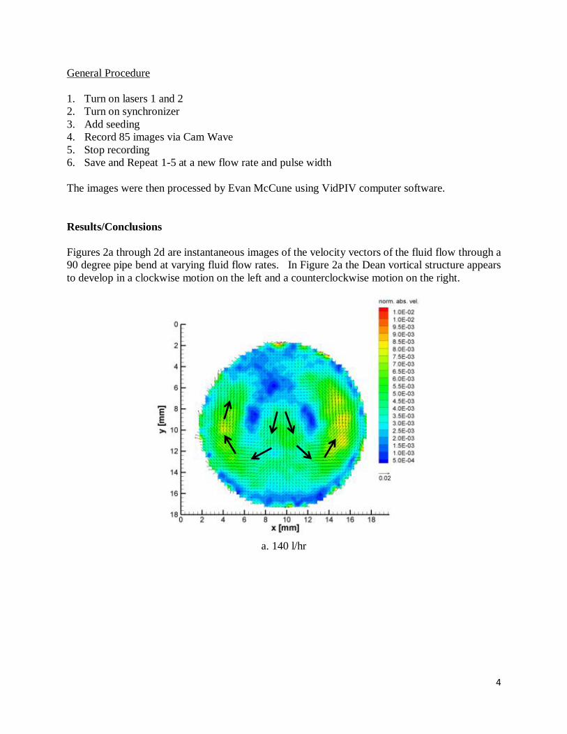
Figures 2a through 2d are instantaneous images of the velocity vectors of the fluid flow through a

90 degree pipe bend at varying fluid flow rates. In Figure 2a the Dean vortical structure appears

to develop in a clockwise motion on the left and a counterclockwise motion on the right.

a. 140 l/hr

5

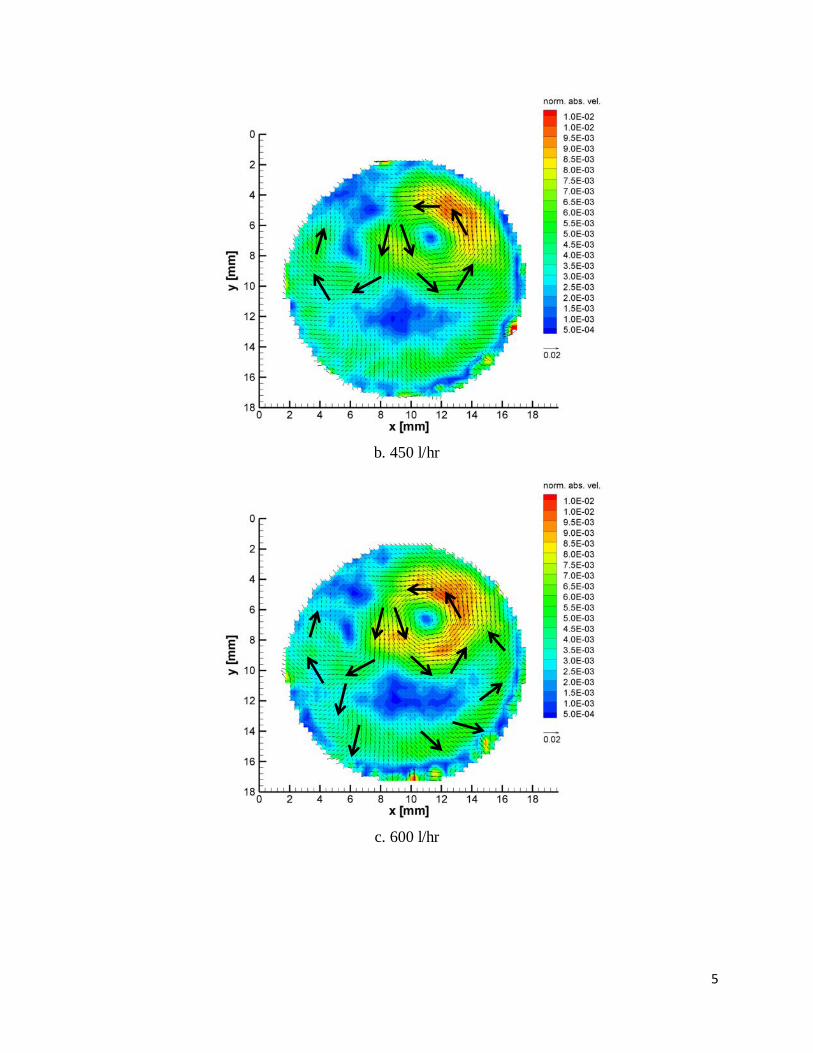
b. 450 l/hr

c. 600 l/hr

6

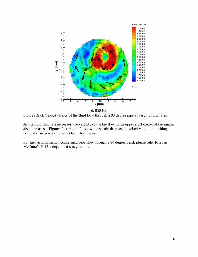
d. 850 l/hr

Figures 2a-d. Velocity fields of the fluid flow through a 90 degree pipe at varying flow rates

As the fluid flow rate increases, the velocity of the the flow in the upper right corner of the images

also increases. Figures 2b through 2d show the steady decrease in velocity and diminishing

vortical structure on the left side of the images.

For further information concerning pipe flow through a 90 degree bend, please refer to Evan

McCune’s 2012 independent study report.

7

Identification of trailing-edge-noise at buffet flows using high-speed PIV

Introduction/Abstract

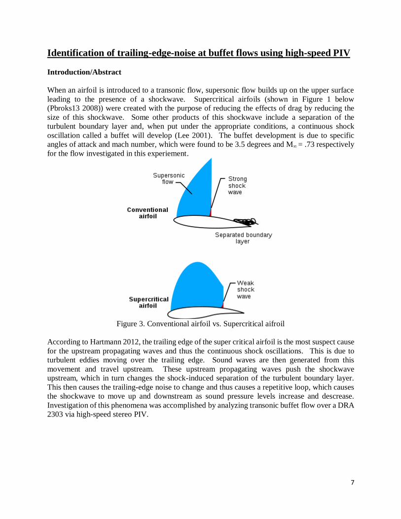
When an airfoil is introduced to a transonic flow, supersonic flow builds up on the upper surface

leading to the presence of a shockwave. Supercritical airfoils (shown in Figure 1 below

(Pbroks13 2008)) were created with the purpose of reducing the effects of drag by reducing the

size of this shockwave. Some other products of this shockwave include a separation of the

turbulent boundary layer and, when put under the appropriate conditions, a continuous shock

oscillation called a buffet will develop (Lee 2001). The buffet development is due to specific

angles of attack and mach number, which were found to be 3.5 degrees and M∞ = .73 respectively

for the flow investigated in this experiement.

Figure 3. Conventional airfoil vs. Supercritical aifroil

According to Hartmann 2012, the trailing edge of the super critical airfoil is the most suspect cause

for the upstream propagating waves and thus the continuous shock oscillations. This is due to

turbulent eddies moving over the trailing edge. Sound waves are then generated from this

movement and travel upstream. These upstream propagating waves push the shockwave

upstream, which in turn changes the shock-induced separation of the turbulent boundary layer.

This then causes the trailing-edge noise to change and thus causes a repetitive loop, which causes

the shockwave to move up and downstream as sound pressure levels increase and descrease.

Investigation of this phenomena was accomplished by analyzing transonic buffet flow over a DRA

2303 via high-speed stereo PIV.

8

Identification of the trailing–edge noise source and upstream propagating waves may be found

upon observation of several periodic patterns including vortical flow structures at the trailing edge.

A phase averaged correlation of the velocity distribution (Hartmann 2012) can aid in identifying

the vortical structures and the distances between them.

√

(1)

Using the two dimensional Q criterion (eqn. 2 below), vortical structures can be observed and their

distinct periodic pattern can be found. Q is the criterion used to identify vortices, as discussed by

Jeong and Hussain 1995, where S is strain and Ω is the rotation tensor.

‖ ‖ ‖ ‖ (2)

It is possible to obtain the frequency of the self sustained shock oscillation using eqn. 3 (Lee 2001)

below,

(

)

(3)

where c represents the chord length, ud and uu are the downstream and upstream propagating

velocities of the pressure fluctuations respectively and xs is the mean shock position. Thus

frequency of the self sustained shock oscillations depend on the speeds of the upstream and

downstream traveling disturbances and the distance from the mean shock location to the trailing

edge. As of today, this approach has neither been verified nor refuted.

Identifying the cause of the buffet flow (and the resulting upstream propagating sound waves) is

important for numerical simulation verification, avoiding resonance frequencies of extremely

flexible and light weight wings required for the future production of more fuel efficient aircrafts.

Therefore the identification of the propagation speeds of the the sound waves is of great interest.

Furthermore, the precise identification of the noise source is essential.

9

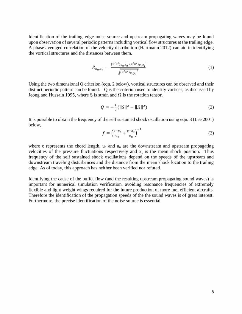
Methods

This experiment was executed using the Trisonic Wind Tunnel at RWTH Aachen University’s

Institute of Aerodynamics. The Trisonic Wind Tunnel (as shown in Figures 4 and 5(Hartmann

2012)) is a customizable vacuum storage tunnel that allows the user to modify the upstream and

down stream cross-sectional areas in order to adjust the Mach number of the fluid flow. The

range of Mach numbers in which the Tunnel can achieve vary from .4 to 3.0.

Figure 4. Trisonic Wind Tunnel

When executing test runs, it is important to take the properties of the fluid (in this case air) into

consideration. In order to properly run the experiment, it is important that the air be dry and

relatively close to room temperature. This is accomplished by using a temperature controlled

laboratory and silica gel to keep the air humidity below 4%. This dry air is then stored in the

reservoir balloon (refer to Figures 4 and 5 (Hartmann 2012)) at the upstream end of the wind

tunnel, where Di-Ethyl-Hexyl-Sebacat (DEHS) tracer particles were added. The DEHS particles

were approximately .6 µm in diameter.

10

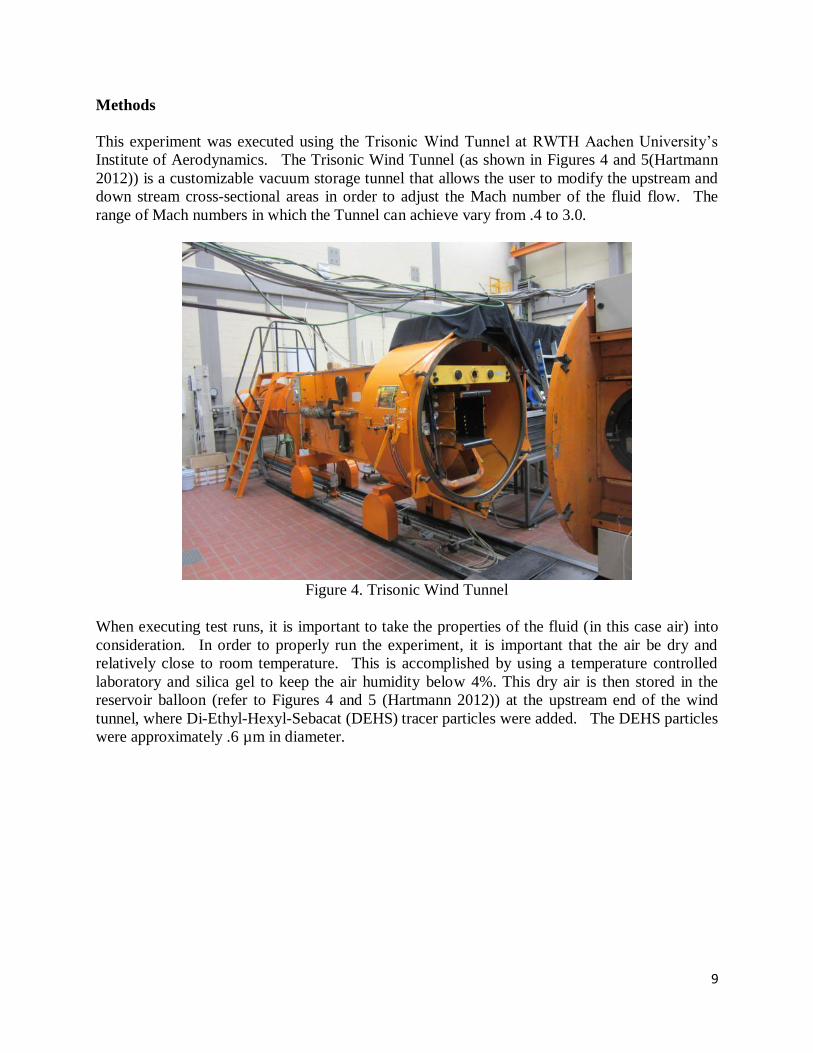
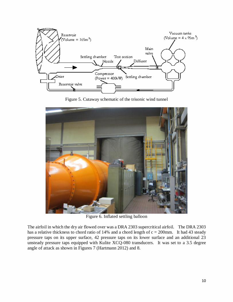
Figure 5. Cutaway schematic of the trisonic wind tunnel

Figure 6. Inflated settling balloon

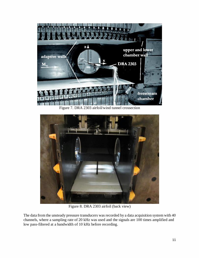
The airfoil in which the dry air flowed over was a DRA 2303 supercritical airfoil. The DRA 2303

has a relative thickness to chord ratio of 14% and a chord length of c = 200mm. It had 43 steady

pressure taps on its upper surface, 42 pressure taps on its lower surface and an additional 23

unsteady pressure taps equipped with Kulite XCQ-080 transducers. It was set to a 3.5 degree

angle of attack as shown in Figures 7 (Hartmann 2012) and 8.

11

Figure 7. DRA 2303 airfoil/wind tunnel crossection

Figure 8. DRA 2303 airfoil (back view)

The data from the unsteady pressure transducers was recorded by a data acquisition system with 40

channels, where a sampling rate of 20 kHz was used and the signals are 100 times amplified and

low pass-filtered at a bandwidth of 10 kHz before recording.

12

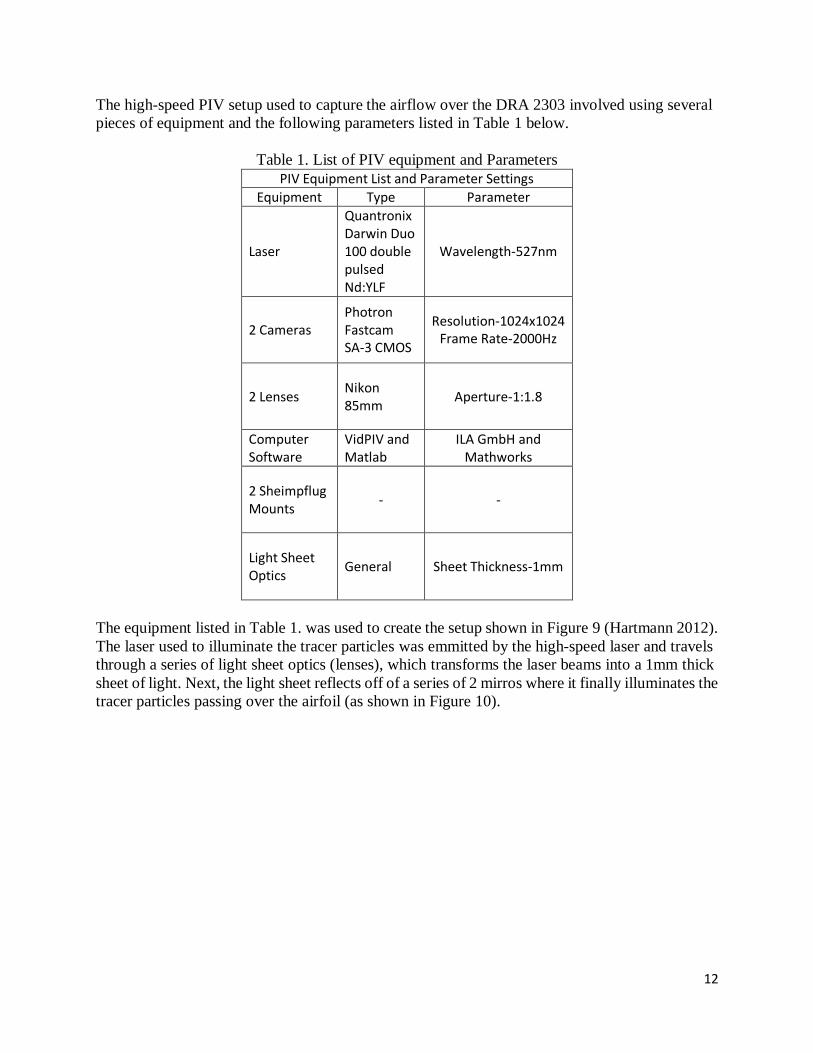
The high-speed PIV setup used to capture the airflow over the DRA 2303 involved using several

pieces of equipment and the following parameters listed in Table 1 below.

Table 1. List of PIV equipment and Parameters

PIV Equipment List and Parameter Settings

Equipment Type Parameter

Laser

Quantronix Darwin Duo 100 double pulsed Nd:YLF

Wavelength-527nm

2 Cameras Photron Fastcam SA-3 CMOS

Resolution-1024x1024 Frame Rate-2000Hz

2 Lenses Nikon 85mm

Aperture-1:1.8

Computer Software

VidPIV and Matlab

ILA GmbH and Mathworks

2 Sheimpflug Mounts

- -

Light Sheet Optics

General Sheet Thickness-1mm

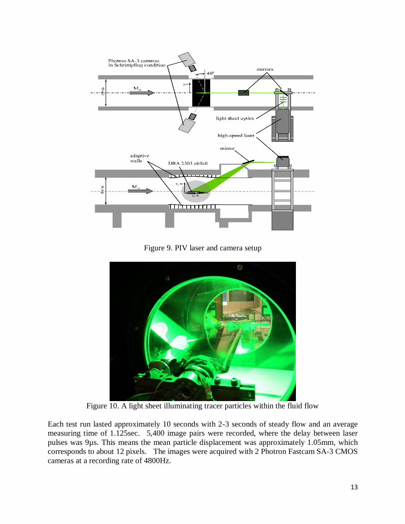
The equipment listed in Table 1. was used to create the setup shown in Figure 9 (Hartmann 2012).

The laser used to illuminate the tracer particles was emmitted by the high-speed laser and travels

through a series of light sheet optics (lenses), which transforms the laser beams into a 1mm thick

sheet of light. Next, the light sheet reflects off of a series of 2 mirros where it finally illuminates the

tracer particles passing over the airfoil (as shown in Figure 10).

13

Figure 9. PIV laser and camera setup

Figure 10. A light sheet illuminating tracer particles within the fluid flow

Each test run lasted approximately 10 seconds with 2-3 seconds of steady flow and an average

measuring time of 1.125sec. 5,400 image pairs were recorded, where the delay between laser

pulses was 9µs. This means the mean particle displacement was approximately 1.05mm, which

corresponds to about 12 pixels. The images were acquired with 2 Photron Fastcam SA-3 CMOS

cameras at a recording rate of 4800Hz.

14

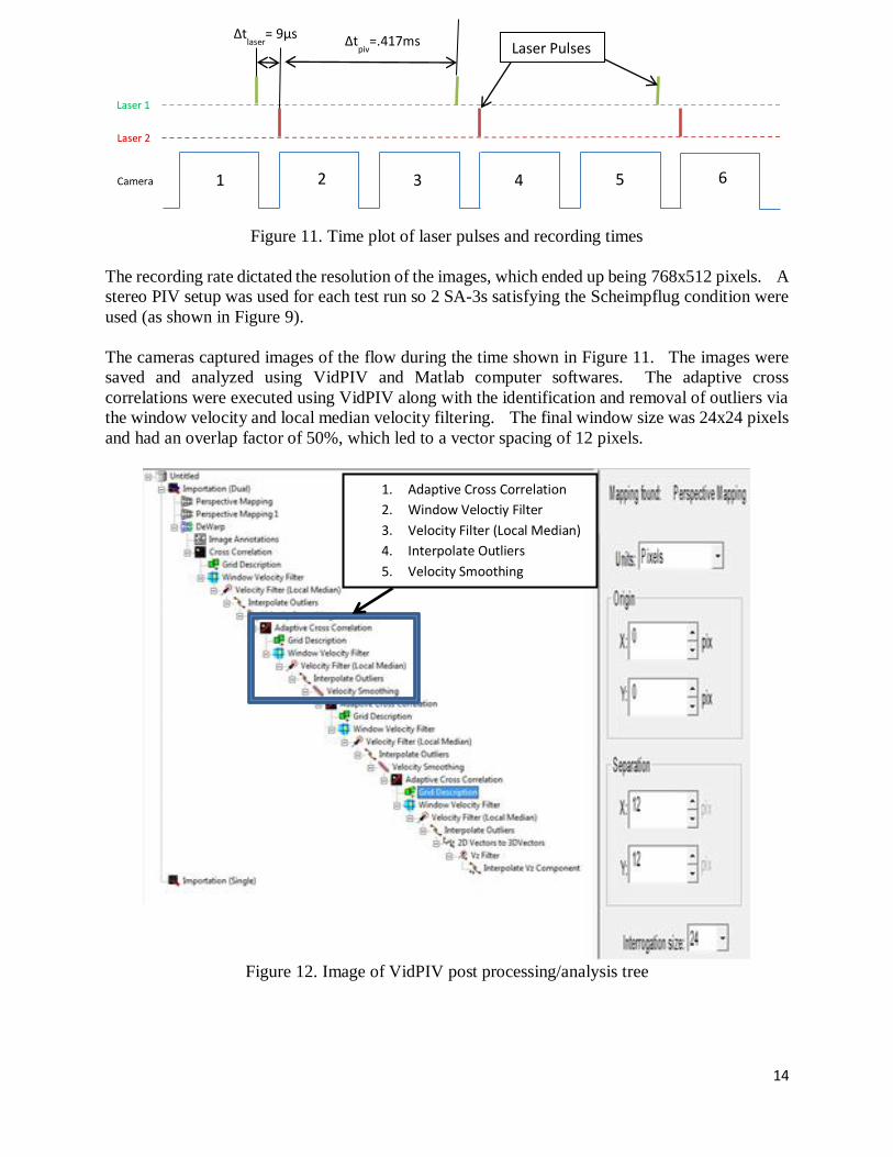
Figure 11. Time plot of laser pulses and recording times

The recording rate dictated the resolution of the images, which ended up being 768x512 pixels. A

stereo PIV setup was used for each test run so 2 SA-3s satisfying the Scheimpflug condition were

used (as shown in Figure 9).

The cameras captured images of the flow during the time shown in Figure 11. The images were

saved and analyzed using VidPIV and Matlab computer softwares. The adaptive cross

correlations were executed using VidPIV along with the identification and removal of outliers via

the window velocity and local median velocity filtering. The final window size was 24x24 pixels

and had an overlap factor of 50%, which led to a vector spacing of 12 pixels.

Figure 12. Image of VidPIV post processing/analysis tree

Camera

Laser 2

Laser 1

1 2 3 4 5 6

∆tlaser

= 9µs ∆tpiv

=.417ms Laser Pulses

1. Adaptive Cross Correlation

2. Window Veloctiy Filter

3. Velocity Filter (Local Median)

4. Interpolate Outliers

5. Velocity Smoothing

15

Results/Discussion

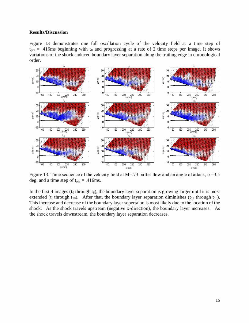
Figure 13 demonstrates one full oscillation cycle of the velocity field at a time step of

tpiv = .416ms beginning with t0 and progressing at a rate of 2 time steps per image. It shows

variations of the shock-induced boundary layer separation along the trailing edge in chronological

order.

Figure 13. Time sequence of the velocity field at M=.73 buffet flow and an angle of attack, α =3.5

deg. and a time step of tpiv = .416ms.

In the first 4 images (t0 through t6), the boundary layer separation is growing larger until it is most

extended (t8 through t10). After that, the boundary layer separation diminishes (t12 through t16).

This increase and decrease of the boundary layer sepertaion is most likely due to the location of the

shock. As the shock travels upstream (negative x-direction), the boundary layer increases. As

the shock travels downstream, the boundary layer separation decreases.

16

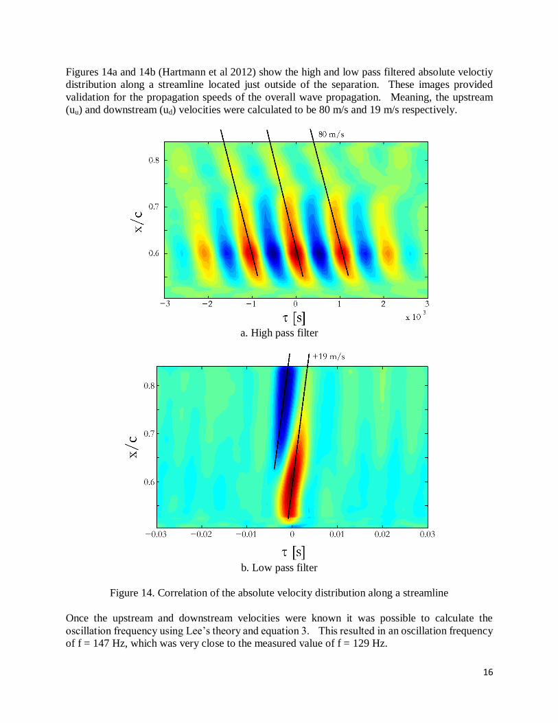
Figures 14a and 14b (Hartmann et al 2012) show the high and low pass filtered absolute veloctiy

distribution along a streamline located just outside of the separation. These images provided

validation for the propagation speeds of the overall wave propagation. Meaning, the upstream

(uu) and downstream (ud) velocities were calculated to be 80 m/s and 19 m/s respectively.

a. High pass filter

b. Low pass filter

Figure 14. Correlation of the absolute velocity distribution along a streamline

Once the upstream and downstream velocities were known it was possible to calculate the

oscillation frequency using Lee’s theory and equation 3. This resulted in an oscillation frequency

of f = 147 Hz, which was very close to the measured value of f = 129 Hz.

17

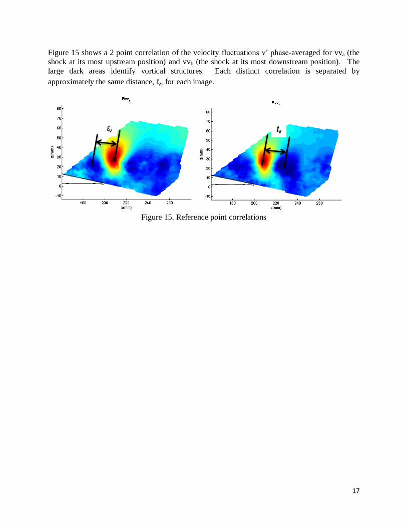
Figure 15 shows a 2 point correlation of the velocity fluctuations v’ phase-averaged for vva (the

shock at its most upstream position) and vvb (the shock at its most downstream position). The

large dark areas identify vortical structures. Each distinct correlation is separated by

approximately the same distance, lv, for each image.

Figure 15. Reference point correlations

lv lv

18

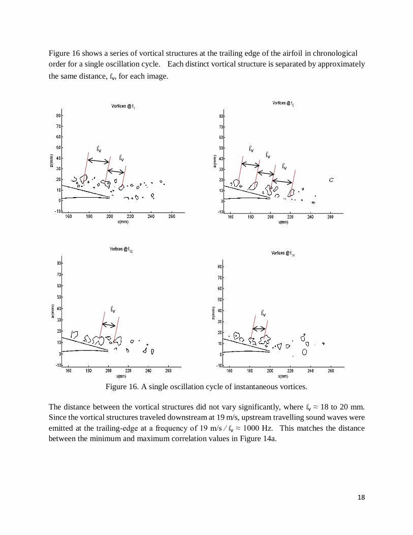
Figure 16 shows a series of vortical structures at the trailing edge of the airfoil in chronological

order for a single oscillation cycle. Each distinct vortical structure is separated by approximately

the same distance, lv, for each image.

Figure 16. A single oscillation cycle of instantaneous vortices.

The distance between the vortical structures did not vary significantly, where lv ≈ 18 to 20 mm.

Since the vortical structures traveled downstream at 19 m/s, upstream travelling sound waves were

emitted at the trailing-edge at a frequency of 19 m/s ∕ lv ≈ 1000 Hz. This matches the distance

between the minimum and maximum correlation values in Figure 14a.

lv lv

lv lv

lv

lv lv

19

Summary and Conclusions

The observation of transonic flow around a DRA 2303 supercritical airfoil issued the investigation

of upstream propagating waves at buffet flow. These observations and analysis of the flow were

possible via high-speed-stereo PIV, VidPIV and Matlab computer softwares. Identifying the

cause of the upstream propagating waves and buffet flow is important for numerical simulation

verification and avoiding resonance frequencies of extremely flexible and light weight wings

required for the future production of more fuel efficient aircrafts.

One supporting observation was obtained from the analysis of the chronological progression of the

boundary layer separation, which unvailed distinct shock location variations. As the shock

traveled upstream, the boundary layer separation increased in size. As the shock traveled

downstream, the boundary layer separation decreased in size. The varying shock location is also

evident when observing the vortical structures. The spacing between them is almost constant,

therefore suggesting noise (sound waves) generated at the trailing edge is the cause of the upstream

propagating waves. The noise level thereby varies with the extension of the separation.

Analysis of the vortical structures and the absolute velocity distribution along a streamline located

just outside of the separation led to the final verification of the upstream propagating waves and

the identification of the trailing edge noise. Since vortical structures traveled downstream at 19

m/s, sound waves were emitted at the trailing-edge at a frequency of 1000 Hz. These values

match the results from Figure 14. Then the sound waves emitted at the trailing edge travelled

upstream, which explains the generation of the upstream waves forming the feedback. Thus the

identification of the trailing-edge-noise and the resulting upstream propagating waves was

accomplished.

20

Acknowledgements

I would like to thank RWTH and the Institute of Aerodynamics for allowing me to take part in this

rewarding experience abroad. I would also like to personally thank Wolfgang Schröder, Axel

Hartmann, Franka Schröder and the rest of the students and staff at the Institute of Aerodynamics

for all their help and generosity.

References

1. Hartmann, Axel. "Experimental Analysis of Wave Propagation at Buffet Flows." Diss.

Rheinisch–Westf¨alischen Technischen Hochschule Aachen, 2012. Print.

2. Hartmann, Axel, Stefan Kallweit, Antje Feldhusen, and Wolfgang Schröder. "Detection of

upstream propagating sound wabes at buffet flow using high-speed PIV.". Aachen: 2012.

Print.

3. Jeong, J. and F. Hussain. On the identification of a vortex. 285. J Fluid Mech, 1995.69-95.

4. Lee, B.H.K. Self-sustained shock oscillations on airfoils at transonic speeds. 37. Progr.

Aerospace Sci., 2001. 147-196. Print.

5. Pbroks13. Airfoils. 2008. Graphic. WikipediaWeb. 27 Jun 2012.

<http://en.wikipedia.org/wiki/File:Airfoils.svg>.

6. Super critical wing. (2002). Retrieved from

<a href="http://encyclopedia2.thefreedictionary.com/Supercritical+airfoil">supercritical

wing</a>