High Resolution Force Measurement System for Lorentz Force ...
107
High Resolution Force Measurement System for Lorentz Force Velocimetry Dissertation zur Erlangung des akademischen Grades Doktoringenieur (Dr.-Ing.) vorgelegt der Fakultät für Maschinenbau der Technischen Universität Ilmenau von Frau M.Sc. Na Yan geboren am 11.08.1988 in Heilongjiang, China Gutachter: Herr Univ.-Prof. Dr.-Ing. habil. Thomas Fröhlich, TU Ilmenau Herr Univ.-Prof. Dr.-Ing. habil. Eberhard Manske, TU Ilmenau Frau Dr.-Ing. Dorothea Knopf, PTB Braunschweig eingereicht am: 07.11.2018 verteidigt am: 26.02.2019 urn:nbn:de:gbv:ilm1-2019000068
Transcript of High Resolution Force Measurement System for Lorentz Force ...

High Resolution Force Measurement System for
Lorentz Force Velocimetry
Dissertation
zur Erlangung des akademischen Grades
Doktoringenieur (Dr.-Ing.)
vorgelegt der
Fakultät für Maschinenbau
der Technischen Universität Ilmenau
von Frau
M.Sc. Na Yan
geboren am 11.08.1988 in Heilongjiang, China
Gutachter: Herr Univ.-Prof. Dr.-Ing. habil. Thomas Fröhlich, TU Ilmenau
Herr Univ.-Prof. Dr.-Ing. habil. Eberhard Manske, TU Ilmenau
Frau Dr.-Ing. Dorothea Knopf, PTB Braunschweig
eingereicht am: 07.11.2018
verteidigt am: 26.02.2019
urn:nbn:de:gbv:ilm1-2019000068


I
Acknowledgments
At first I sincerely would like to express my thanks to Prof. Thomas Fröhlich for his encouragement
and supervision. From him, I have learned the correct way to do scientific researches. Many thanks to
Dr. Suren Vasilyan, Dr. Michael Kühnel, Dr. Ilko Rahneberg and Dr. Jan Schleichert for the
discussions at the earlier stages of the work. I would like to thank Dr. Uwe Gerhardt for providing
many electronic components. I am also grateful for my colleagues from the Institute of Process
Measurement and Sensor Technology for providing me a supportive working environment for
developing this thesis. The appreciation is also extended to Mathias Röser and Jürgen Bretschneider
for their technical supports, to Helge Mammen, Vinzenz Ullmann, Norbert Rogge and Dr. Marc
Schalles for lending me the devices. Without the people mentioned above, this work would never have
been successfully finished within these three years.
Moreover, I would like to express my special appreciation to my parents (Xiulan and Peisheng) and all
the family members (especially Bingyu and Kegong) for their support and guidance during all my life.
Sincerely thanks to my husband Kuan for always being my strong backup since I started my work as a
PhD student.
Additionally, I would like to thank everyone who have encouraged me, smiled to me after my talks
and during the conferences…
Finally, I would like to express my thanks to my colleagues from the whole research training group
"Lorentz Force Velocimetry and Lorentz Force Eddy Current Testing" supported by Deutsche
Forschungsgemeinschaft (DFG).


III
Kurzfassung
Die Lorentzkraft-Anemometrie wurde als neuartige Methode für die berührungslose Geschwindig-
keitsmessungen leitfähiger Strömungen entwickelt. Die induzierte Lorentzkraft ist proportional zur
Strömungsgeschwindigkeit. Mit einem Kraftmesssystem kann die Reaktionskraft der induzierten
Lorentzkraft, die auf das integrierte Magnetsystem wirkt, gemessen werden. Dadurch kann die
Strömungsgeschwindigkeit bestimmt werden. Die Eigenschaften der Geschwindigkeitsmessung
hängen von den Eigenschaften des Kraftmesssystems ab. Bei Fluiden mit geringer elektrischer
Leitfähigkeit, wie z.B. Elektrolyten, liegt die erzeugte Lorentzkraft im Bereich von Mikronewton und
darunter. Das Kraftmesssystem unterstützt eine Masse eines Magnetsystems von ca. 1 kg. Deshalb ist
das Ziel dieser Arbeit ein Kraftmesssystem zu entwickeln, welches auf der einen Seite eine verbesserte
Kraftauflösung in horizontaler Richtung für niedrigleitende Elektrolyte aufweist und auf der anderen
Seite die Tragfähigkeit der Eigenlast von über 1 kg zur Unterstützung des integrierten Magnetsystems
gewährleistet.
In vorherigen Arbeiten wurde die Wägezelle nach dem Prinzip der elektromagnetischen Kraft-
kompensation (EMK-Wägzelle) in aufgehängter Konfiguration mit dem 1 kg Magnetsystem zur
Messung der Lorentzkraft verwendet. Basierend auf verschiedenen Experimenten in dieser vorge-
stellten Arbeit wird festgestellt, dass aufgrund des mechanischen Aufbaus sowohl Neigungs-
empfindlichkeit als auch Steifigkeit der EMK-Wägezelle stark von der genutzten Konfiguration und
dem Gewicht der unterstützten Eigenlast abhängig sind. Um die durch diese Abhängigkeiten
verursachten Einflüsse zu minimieren, wird ein Torsionskraftmesssystem basierend auf dem Prinzip
der Torsionswaage entwickelt. Diese ist theoretisch neigungsunempfindlich und behält bei
unterschiedlichen Eigenlasten eine konstante Steifigkeit bei.
Die Auslenkungsmessungen werden verwendet, um die Ausgangsspannung des Torsionskraft-
messsystems sowohl in Positionswerten als auch in Kraftwerten zu kalibrieren. Ein Closed-Loop-
Betriebsmodus wird mithilfe eines PID-Reglers aufgebaut, mit dem die Grenzfrequenz von 0,002 Hz
auf 0,1 Hz verbessert wird. Ein spezialangefertigter kapazitiver Aktor wird entwickelt, um eine
rückführbare elektrostatische Kraft zu erzeugen, die anstelle der elektromagnetischen Kraft verwendet
werden kann. Um die elektrostatische Kraft zu kalibrieren, werden drei Methoden genutzt: (a) durch
Messung des Kapazitätsgradienten; (b) durch Vergleich mit einer elektromagnetischen Kraft und (c)
durch Messung des induzierten Stroms in einem Velocity-Modus. Bei der Datenauswertung wird eine
numerische Verarbeitung mit Newton-Polynominterpolation durchgeführt, um die thermischen und
seismischen Störungen und Driften während der Messungen zu schätzen und zu korrigieren. Im
Vergleich zu vorherigen Arbeiten, wo die Kraftauflösung auf 20 nN und die Eigenlast auf 3 kg
begrenzt waren, ist das Torsionskraftmesssystem in der Lage, Kräfte bis zu 2 nN aufzulösen und eine
Eigenlast bis zu 10 kg zu tragen.
Schließlich wird die sogenannte Halb-Trocken-Kalibrierung am Torsionskraftmesssystem durch-
geführt. Die Messempfindlichkeit wird für unterschiedliche Leitfähigkeiten ermittelt. Basierend auf
den experimentellen Ergebnissen, zeigt das Torsionskraftmesssystem das Potential, um Messungen
mit weiter geringerer Leitfähigkeit bis hinunter zu 0.0064 S m-1
durchzuführen.

V
Abstract
The Lorentz force velocimetry (LFV) was introduced as a novel method for non-contact velocity
measurements of electrically conducting flows. The induced Lorentz force is proportional to the flow
velocity. Using the force measurement system (FMS), the reaction force of the induced Lorentz force
that acts on the integrated magnet system can be measured, the velocity of the moving flow can be
thereby determined. The characteristics of the measured flow velocity depend on the properties of the
FMS. For weakly electrically conducting fluids like electrolytes, the induced Lorentz force is in the
range of micronewton and below. The mass of the magnet system supported by the FMS is
approximately 1 kg. Therefore, the aim of this work is to develop a FMS with the improved force
resolution in horizontal direction for weakly conducting electrolytes, and also with the dead load
capacity of over 1 kg for supporting the integrated magnet system.
In previously developed FMSs, the electromagnetic force compensation (EMFC) weighing cell was
used in its suspended configuration carrying the 1 kg magnet system to measure the Lorentz force.
Based on various experiments in the presented work, it is found that due to its mechanical structure,
the tilt sensitivity and the stiffness of the EMFC system are strongly dependent from the configuration
it is used and the weight of dead load it supports. In order to minimize the influences caused by the
dependency, the torsion force measurement system (TFMS), which is theoretically tilt-insensitive as
well as retains a constant stiffness with different applied dead load values, is developed in this work
based on the principle of torsion balance.
The deflection measurement as a traceable method is introduced to calibrate the output of the TFMS
into positioning as well as force values. The closed-loop operation mode is built based on PID-
controller, by which the cutoff frequency is improved from lower than 0.002 Hz to 0.1 Hz. A
customized capacitive actuator is set up to create traceable electrostatic force (ESF), which is a
reasonable replacement of the electromagnetic force (EMF). Then, the ESF is calibrated using three
methods: (a) by measuring capacitance gradient; (b) by comparing with the EMF and (c) by measuring
the induced current in a velocity mode. Numerical processing using newton's polynomial interpolation
is carried out in the data evaluation to estimate and compensate the thermal and seismic drifts during
the measurements. In comparison with previous work where the force measurement resolution was
limited to 20 nN and dead load up to 3 kg, the TFMS is able to resolve forces down to 2 nN and also
makes it possible to carry the dead load up to 10 kg.
Finally, the so-called semi-dry calibration is carried out on the TFMS. The measuring sensitivity is
obtained in respect to different conductivity values. Based on the experimental results, the TFMS
shows a potential to implement velocity measurements with further lower conductivity down to
0.0064 S m-1
.


VII
Contents
1. Introduction ..................................................................................................................................... 1
1.1 Lorentz Force Velocimetry...................................................................................................... 1
1.2 State-of-the-Art of the FMSs ................................................................................................... 2
1.2.1 Background ........................................................................................................................ 2
1.2.2 FMSs developed for Lorentz force velocimetry ................................................................. 6
1.3 Summary and scope of the work ............................................................................................. 8
2. Investigation on the EMFC weighing cell ..................................................................................... 10
2.1 Tilt sensitivity of the EMFC weighing cell ........................................................................... 11
2.2 Stiffness of the EMFC weighing cell .................................................................................... 18
2.3 Summary ............................................................................................................................... 24
3. Design concept of torsion force measurement system .................................................................. 26
3.1 Initial idea and theoretical calculation ................................................................................... 26
3.2 Plane wheel with dead load ................................................................................................... 29
3.3 Flexible bearing support ........................................................................................................ 29
3.3.1 Flexible bearing hinge ...................................................................................................... 29
3.3.2 Conical coupling ............................................................................................................... 30
3.4 Positioning sensor .................................................................................................................. 31
3.5 Adjustment and safety components ....................................................................................... 33
3.6 Summary ............................................................................................................................... 33
4. TFMS in the open-loop operation mode ....................................................................................... 35
4.1 Position calibration using deflection method ........................................................................ 35
4.1.1 Force/ motion actuation using deflection method ............................................................ 36
4.1.2 Experimental facility ........................................................................................................ 37
4.1.3 Measurements ................................................................................................................... 38
4.2 Force calibration using deflection method ............................................................................ 40
4.2.1 Adjustment of the tilt sensitivity ...................................................................................... 40
4.2.2 Force calibration ............................................................................................................... 42
VIII
4.2.3 Uncertainty discussion ...................................................................................................... 45
4.3 System identification ............................................................................................................. 46
4.4 Summary ............................................................................................................................... 48
5. TFMS in the closed-loop operation mode ..................................................................................... 50
5.1 Setting up PID-controller using electromagnetic force ......................................................... 51
5.2 Setting up electrostatic force generator ................................................................................. 55
5.3 Calibration of electrostatic force ........................................................................................... 57
5.3.1 Three methods to calibrate the electrostatic force ............................................................ 58
5.3.2 Discussion and uncertainty budget .................................................................................. 62
5.4 Test of the dynamic behavior ................................................................................................ 64
5.5 Test of force resolution .......................................................................................................... 66
5.6 Summary ............................................................................................................................... 69
6. Lorentz force measurement ........................................................................................................... 72
6.1 Experimental facility ............................................................................................................. 72
6.2 Semi-dry calibration of the TFMS ........................................................................................ 75
6.3 Summary ............................................................................................................................... 79
7. Conclusions and Outlook .............................................................................................................. 81
Appendix A Calibration of the NI9239 ................................................................................................. 85
Appendix B Geometrical parameters .................................................................................................... 86
Bibliography .......................................................................................................................................... 88
Erklärung ............................................................................................................................................... 93
IX
Nomenclature
Acronyms
AFM Atomic Force Microscopy
COG Center of Gravity
DFMS Differential Force Measurement System
EFB Electrostatic Force Balance
ESF Electrostatic Force
EMF Electromagnetic Force
EMFC Electromagnetic Force Compensation
FMS Force Measurement System
HTS High-Temperature Superconducting
LFV Lorentz Force Velocimetry
NPI Newton's Polynomial Interpolation
PCB Printed Circuit Board
PFMS Pendulum Force Measurement System
PP Pivot Point
TFMS Torsion Force Measurement System
Variables
FL [N] Lorentz force
FL'
[N] Reaction force of the Lorentz force
σ [S m-1
] Electrical conductivity
v [m s-1
] Flow velocity
B [T] Magnetic flux density
Fm [N] Deadweight force
Fc [N] Compensation force

X
Ic [A] Compensation current
l [m] Length of the coil wire
Fa [N] Actuation force
Ft [N] Tilt force
Fes [N] Electrostatic force
Fem [N] Electromagnetic force
EMFC
m1
[kg]
Deadweight at the position of weighing pan of the EMFC weighing cell
m2 [kg] Deadweight at the position of counterweight of the EMFC weighing cell
∆m [kg] Additionally applied mass on the weighing cell
α [rad] Tilt angle of the system
L1 [m] Arm length of the deadweight m1
L2 [m] Arm length of the deadweight m2
[rad] Misalignment angle of the EMFC on the tilt stage
Ls [m] Distance between the pivot and positioning sensor
Lm [m] Distance between the pivot and the voice coil actuator
s [m] Linear displacement at the positioning sensor
β [rad] Angular defection of the lever arm
Ms [N m] Torque caused by the spring constant of the weighing cell Cp and the angular
deflection β
Cs [N m-1
] Linear stiffness of the weighing cell
Cr [N rad-1
] Rotational stiffness of the weighing cell
Cp [N m rad-1
] Spring constant of the mechanical structure of the weighing cell
TFMS
LT1 [m] Distance between the rotational axis and the non-magnetic dummy
LT2 [m] Distance between the rotational axis and the magnet system (or replacement
dummy)

XI
R [m] Distance between the rotational axis and the positioning sensor
Ct [N m-1
] Effective stiffness of the TFMS for measuring Lorentz force
Cb [N m rad-1
] Spring constant of the commercial flexible bearing hinge
fn [Hz] Undamped natural frequency
J [kg m2] The moment of inertia
θ [rad] Rotational angle of the TFMS
UP [V] Output voltage of positioning sensor
Kps [rad V-1
] Position calibration factor
Lx [m] Displacement of COG from the PP in x-direction
Ly [m] Displacement of COG from the PP in y-direction
αx [rad] Tilt angle around x-axis
αy [rad] Tilt angle around y-axis
Mt [N m] Torque caused by the tilt sensitivity
Tx [rad rad-1
] Tilt sensitivity around x-axis
Ty [rad rad-1
] Tilt sensitivity around y-axis
Km [N m V-1
] Convert factor transferring the voltage value into torque value
KF [N V-1
] Force calibration factor
TP [s] Peak time
ζ -- Damping ratio
ωn [rad s-1
] Undamped natural frequency (angular)
ωd [rad s-1
] Damped natural frequency (angular)
τ [s] Settling time
UP0 [V] Defined voltage value, given in the PID-controller, used to define the null
position of the plane wheel
Kvc [N A-1
] Force constant of the commercial voice coil actuator
Kes [N V-2
] Calibration factor of electrostatic force
Ua [V] Actuation voltage across the two electrodes of the customized capacitor
A [mm2] Effective cross section area of the capacitor
C [pF] Capacitance value
dx [µm] Distance between the two electrodes of the customized capacitor
d0 [µm] Distance between the two electrodes of the customized capacitor when UP0 = 0

XII
ds [µm] Change of the distance between the two electrodes of the customized capacitor
ds [µm s-1
] Moving velocity of one electrode of the customized capacitor
Ua0 [V] Pre-voltage supplied across the customized capacitive actuator
Da [mm] Diameter of the annular pipe

1. Introduction
Dissertation Na Yan 1
1. Introduction
In this chapter, the principle and application of the Lorentz Force Velocimetry (LFV) are introduced
briefly in section 1.1. In section 1.2, systems showing the state-of-the-art in force metrology are
presented and several other related force measurement systems (FMSs) developed especially for the
LFV are reviewed. In section 1.3, the scope of the work presented in the thesis is demonstrated.
1.1 Lorentz Force Velocimetry
The Lorentz Force Velocimetry (LFV) has been introduced in many works [1-8] as a non-contact
technique to measure the mean flow velocity of electrically conducting fluid flows. Compared to
optical, magneto-inductive and ultrasound techniques of flowmeters, the LFV as a contactless method
is more desirable for applications in cases when the pipes are opaque and hot and/or the fluids are
aggressive. The LFV setup is made up of three main parts as illustrated with the simplified principle
sketch in figure 1.1, they are: ① flow channel with moving conducting fluid inside, the mean flow
velocity v is expected to be determined; ② magnet system to generate the required magnetic field
over the channel and ③ force measurement system (FMS) carrying the magnet system and measuring
the reaction force of the induced Lorentz force. The channel is exposed in the magnetic field with the
magnetic flux density B. In the channel moves the conducting fluid with velocity v and electrical
conductivity σ across magnetic field lines. The interaction of the magnetic field with the induced eddy
current leads to the braking force FL in the direction to slow down the motion of the fluid. The force FL
is proportional to the velocity v, the electrical conductivity σ and the second power of the magnetic
flux density B2, and can be described with the equation (1.1) as introduced in [1].
2
LF c v B K v (1.1)
The factor c is a constant which depends on the geometry of the magnet system and the geometry of
the flow. According to the Newton's Third Law, a force equals to the braking force FL acting in the
opposite direction is generated upon the magnet system. As illustrated in figure 1.1, the reaction force
FL' can be detected by the FMS. When the factor K in equation (1.1) is known, namely, after the
system is calibrated with known velocity values, the flow velocity v can be obtained by the measured
force from FMS. Moreover, this principle presented by equation (1.1) can also be applied in testing
defects in materials by measuring conductivity σ when the velocity is a constant value [9].
The focus of this work is to develop the FMS to improve the Lorentz force measurement with
electrolytes, whose electrical conductivity are in the range of 10−6
S m-1
to 102 S m
-1. The currently
used magnet system is a Halbach-array with the mass of approximately 1 kg causing the deadweight
force of approximately 10 N [10]. The flow velocity in practical application is lower than 5 m s-1
with
the magnetic field up to 1.5 T [2, 7, 11]. Thus, the induced Lorentz force is approximately in the range
of micronewton and below. Hence, the aim of this work is to improve the force resolution of the FMS

1. Introduction
2 Dissertation Na Yan
in horizontal direction in order to perform measurement with electrolytes, and maintain the dead load
capacity of over 1 kg for carrying the unavoidable dead load caused by the magnet system.
Figure 1.1: Simplified principle sketch of Lorentz Force Velocimetry with integrated channel, magnet
system and FMS (side view).
1.2 State-of-the-Art of the FMSs
1.2.1 Background
Nowadays growing trend for measurement and calibration of small forces is in the field of
nanotechnology and nanometrology [12]. Apart from the LFV framework, the investigations of the
force in micro- and nanonewton are also being in the active focus of most of the national metrological
institutes (NMIs). In this section several FMSs related closely to this work and showing the state-of-
the-art are introduced.
Force is one of the derived units in the International System of Units (SI Units), using the combination
of base SI units of mass ([kg]) and local gravity ([m] and [s]). At present the unit of mass is defined by
the artefact international prototype of kilogram (IPK), which is conserved at the International Bureau
of Weights and Measures (BIPM) since 1889. In comparisons with the IPK through a hierarchical
system, the unit of mass is disseminated throughout the world to NMIs, to laboratories, to industries,
to instruments and sensors, as well as to trades. Multiples and submultiples of one kilogram are also
realized by artefacts manufactured in different shapes and sizes, which are well known as mass
standards. By using mass standards, deadweight forces can be created and calibration measurements
can be performed on different type of sensors. However, there is a limit for providing small forces
using deadweight force such as the traceable mass artefact in the US National Institute of Standard and
Technology (NIST) is down to 0.5 mg corresponding to approximately 5 µN [12], which is still three
orders of magnitude larger than the demand for measuring and calibration of forces in nanonewtons.
Thus, systems are being developed in most NMIs for realization and measuring small force values.
a) Electrostatic force balance
In 2003, NIST reported on the realization of micro force below 5 µN using electrostatic force balance
(EFB), by which the comparison between mechanically and electrically divided forces up to 300 µN
with the resolution of 15 nN is possible [13]. In 2016, with the same principle of the EFB, NIST
.
z
x yFlow
FMS
Magnet Channel
FLFL
B
Eddy current
‚

1. Introduction
Dissertation Na Yan 3
reported force resolution on the order of piconewtons [14]. The National Physical Laboratory in UK
(NPL) designed a primary low force balance via electrical and dimensional measurements and
achieved the resolution of 50 pN [15]. The mechanical structures of EFB facilities differ from each
application but the main parts remain similar as illustrated in figure 1.2. The parallelogram balance
structure (1) carries the inner cylinder electrode (3), to which the outer cylinder electrode (4) is aligned
coaxially. As the inner electrode is free to translate together with the parallelogram mechanism along
z-axis, while the outer electrode is fixed rigidly on the base frame, the overlap of the two electrodes
varies and leads to the electrostatic force Fes with the voltage U applied across the two electrodes, as
equation (1.2) shows:
2 21
2es es
dCF U K U
dz (1.2)
dC/dz indicates the capacitance gradient. When the two cylindrical electrodes are perfectly aligned
coaxially, the capacitance C is linear to the overlap by using this kind of geometrical structure, which
indicates that the capacitance gradient is a constant value and is described by Kes as the constant force
factor.
Figure 1.2: Schematic of electrostatic force balance components: (1) Parallelogram balance
mechanism; (2) Mass/load pan; (3) Inner cylindrical electrode (cross section); (4) Outer
cylindrical electrode (cross section); (5) Interferometer for measuring displacement and
(6) base frame. The structure is drawn according to the facilities described in [14-15].
The EFB operates with null balance principle. Deadweight forces Fm acting on the mass/load pan (2)
causes the displacement of the inner electrode, which can be detected by the interferometer (5). Due to
this displacement, the voltage value U across the two electrodes is able to be calculated and applied to
the capacitor to generate the electrostatic force Fes compensating Fm and maintaining the balance at its
null position. Thus, the electrostatic force between the two electrodes indicates the force Fm as
described by equation (1.3), where m is the applied mass causing deadweight force, g is the local
gravitational acceleration, UN and UL indicate the required electrical voltage to maintain the balance at
null position before and after loading respectively.
2 2( )m es es L NF m g F K U U (1.3)
Fm(1) (2)
(3)
(4)
(5)
(6)
.
z
xy
g
Fes

1. Introduction
4 Dissertation Na Yan
Base on the common structure, derived setups were developed to adapt to local conditions. In [16], an
auxiliary capacitor is assembled on the parallelogram linkage for controlling the motion of the balance
during measuring the capacitance gradient of the main capacitor. Instead of using inner and outer
cylindrical electrodes, plate-shaped electrodes are used in [17] which enables actuate electrostatic
force as well as sense deflection with one structure. While the cylindrical capacitor is kept, the
parallelogram balance mechanism is replaced by a high-sensitive lever mechanism with torsion rod in
[18] to decrease the stiffness of the system.
b) Electromagnetic force compensation balance
Besides the investigations in the NIMs and other metrological institutes, the technique of small force
measurements is also continuously being developed in industries. The commercial electromagnetic
force compensation (EMFC) balances are based on the weighing cell illustrated in figure 1.3 with
monolithic parallelogram mechanism (2) and operate with null balance principle.
Figure 1.3: Schematic of EMFC weighing cell: (1) Mass/load pan; (2) Parallelogram mechanism with
elliptical notch flexures; (3) Transmission lever; (4) Optical positioning sensor; (5) Control
system; (6) Electromagnetic actuator; (7) Counterweight.
The deadweight force Fm of the object acts on the load pan (1) and causes the deflection of the
transmission lever (3). The movement of the lever is continuously recorded by the positioning sensor
(4) with the output voltage U(t). To compensate the deflection, the compensation current Ic is
calculated by the controller due to U(t) and then transferred to the coil wire of the electromagnetic
actuator (6) to generate the electromagnetic force Fc due to equation (1.4). The electromagnetic force
as the compensation force brings the transmission lever back to the null position. l and B indicate the
length of the coil wire and the magnetic flux density of the electromagnetic actuator.
c cF I l B (1.4)
Using this principle, the ultra-micro EMFC balances developed in Sartorius Lab Instrument GmbH
can reach a readability of 0.1 µg, roughly corresponding to forces of < 1 nN, at a weighing capacity of
2 g. Apart from comparing with deadweight force as a balance, the EMFC weighing cell is also used
in combination with other high-precision mechanisms for other applications. In the National
Metrology Institute of Germany (PTB) and Korea (KRISS), piezo actuator deflects the cantilever on
.
z
xy
gSN
U(t)
controller
Ic
Fc
Fm
(1)
(2)(4)(5)
(6) (7)
(3)

1. Introduction
Dissertation Na Yan 5
the EMFC weighing cell to determine the stiffness of the cantilever used in atomic force microscopy
(AFM) [17]. Another similar mode was also carried out in technical university of Ilmenau: instead of
moving the cantilever with the piezo actuator, the load pan is set into controllable motion by the
internal voice coil actuator and probes the fixed cantilever. With the defection measured by
interferometer and the force measured by the weighing cell, the stiffness can be ascertained [19]. As a
derived application utilizing the tilt sensitivity of the EMFC weighing cell, an inclinometer was
developed with the standard deviation of the angle of 3.4 nrad ~7.1 nrad depending on the used filter
[20].
Although the electrostatic force and electromagnetic force are introduced above with the facilities to
measure vertical directed deadweight forces, actuation forces in other directions can also be induced
using the principle indicated in equation (1.2) and (1.4), such as forces in the horizontal plane are
applied on the system developed in this work. The performance of the electrostatic- and
electromagnetic forces related to this work is further described in chapter 5.
Apart from measuring deadweight forces, horizontally directed forces are also under investigation in
several metrological institutes. Similar to the facilities introduced above, the horizontal forces are also
determined by detecting the displacement caused by external forces using optical metrology. Common
mechanisms to enable the displacement in horizontal plane are torsion balance and suspended
pendulum.
c) Torsion balance
The concept of torsion balance is well known as the experiment was carried out by Henry Cavendish
in 1798 to measure the gravitational force between two masses. Nowadays the mechanisms based on
torsion balance principle are still widely used with the aim to improve the uncertainty of the
gravitational constant G. At BIPM the apparatus was designed with four source masses, each of which
weights approximately 11 kg and four test masses each of which weights approximately 1.2 kg on a
torsion disc suspended by a wide torsion strip [21]. The deflection of the test masses is recorded by
autocollimators, by which the achieved uncertainty is 25 ppm in the measured G [21]. Similar facility
was introduced in [22] where only two test masses and two source masses were used. In that work two
methods for generating horizontally directed forces were used, namely, using radiation pressure for
generating optical force with maximum force of 10 nN and using capacitive actuator for generating
electrostatic force in the range of ± 50 nN. In the PhD work of Wagner [23], a rotating torsion balance
was used to test the weak equivalence principle. Based on the torsion balance principle, a FMS is
developed in this work and is further introduced in chapter 3.
d) Suspended pendulum
Besides of using torsion balance, the gravitational constant G can also be determined using beam
balance with an achieved uncertainty of 32.8 ppm [24] or using the pendulum mechanism. In [25] two
bobs made of oxygen-free copper as test masses (each 780 g) are suspended with four wires. Four
source masses can move to the outer position and inner position with the help of air bearings. As a
result, the change of gravitational force on each test masse of 480 nN leads to the separation change,
which is detected by the Fabry-Perot interferometer [25]. Using the laser interferometric measurement
and such pendulum, the uncertainty of 15 ppm in the measured G value was obtained.

1. Introduction
6 Dissertation Na Yan
At PTB, a nanonewton force facility with two identical disc-pendulums was introduced, one of which
measures the target force and the other one works as the reference to measure and compensate the
errors caused by thermal drift/tilt and seismic noise. Using electrostatic force as compensation force,
the facility in PTB can measure the force of 1 nN with the measurement uncertainty of 5% [26].
The introduction above is not a full illustration of all systems indicating the state-of-the-art FMSs in
small force metrology. There are other high-resolution facilities and researches such as AFM and
investigations based on photon pressure forces.
The setups and force measurement principles introduced above are related closely to the FMSs which
have been designed for the Lorentz force measurement in the LFV application, later in section 1.2.2
they will be introduced.
1.2.2 FMSs developed for Lorentz force velocimetry
As introduced in section 1.1, to adapt to the LFV application, the FMSs have been continuously
developed and improved in the last several years with the following main requirements:
a) Force measurement in horizontal plane;
b) High resolution in the range of micro- and nanonewton;
c) High capacity for supporting dead load of over 1 kg.
Initially in [1], the LFV was introduced with a focus on narrow field of application as in metallurgy,
where the electrical conductivity of the fluid is on the order of 106 S m
-1 and the measured Lorentz
force is in the range of millinewton and newton. Then, the LFV was transformed into a universal
flowmeter which is also applicable for weakly conductive liquids by improving the FMS as well as
magnet system. In [3] the FMS was developed with the magnet system carried by a four-wire-
suspension pendulum depicted in figure 1.4 (a). The magnet system consists of two identical NdFeB
permanent magnets with a total mass of 1.286 kg, which is attached to the supporting frame by four
tungsten wires with a diameter of 125 µm and length of 0.55 m. The displacement x of the magnet
system caused by the force FL' is measured by a laser interferometer. The force value can be calculated
from the displacement by FL' = k · x, where k indicates the stiffness of the pendulum-FMS (PFMS)
depending on the mass and length of the pendulum. Using this PFMS, experiments on salt water with
electrical conductivity of 2.3 S m-1
, 4.0 S m-1
and 6.2 S m-1
were carried out, and the measurement
results demonstrated agreement with the simulation.
Subsequently, a robust system was introduced by replacing the pendulum with a single commercial
EMFC weighing cell (see figure 1.3) with its suspended configuration illustrated in figure 1.4 (b) [27].
The parallelogram mechanism of the EMFC weighing cell has a good effect to restrict the
displacement of the magnet system along x-axis. With the EMFC weighing cell, measurements with
both open-loop operation mode where force value is calculated from displacement similar to PFMS;
and closed-loop operation mode where the displacement caused by the external force is compensated
back to null position, can be carried out to measure the reaction force of the Lorentz force. The
induced Lorentz forces generated by flows with velocity of 0 < v ≤ 2.8 m s-1
and electrical
conductivity of 2 ≤ σ ≤ 6 S m-1
were measured with the single EMFC system in combination with
1. Introduction
Dissertation Na Yan 7
conventional magnet system as well as magnets arranged in Halbach-arrays. The relative uncertainty
in the measured force with both magnet systems is lower than ± 1% (confidence level k = 2).
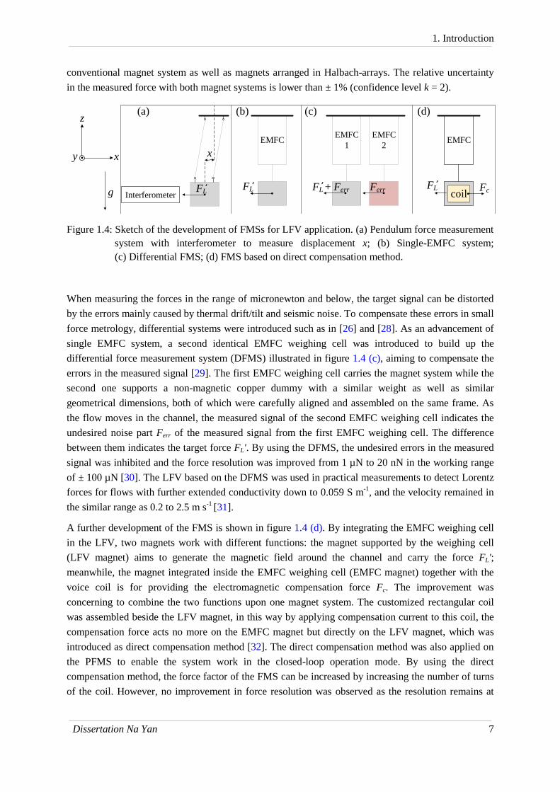
Figure 1.4: Sketch of the development of FMSs for LFV application. (a) Pendulum force measurement
system with interferometer to measure displacement x; (b) Single-EMFC system;
(c) Differential FMS; (d) FMS based on direct compensation method.
When measuring the forces in the range of micronewton and below, the target signal can be distorted
by the errors mainly caused by thermal drift/tilt and seismic noise. To compensate these errors in small
force metrology, differential systems were introduced such as in [26] and [28]. As an advancement of
single EMFC system, a second identical EMFC weighing cell was introduced to build up the
differential force measurement system (DFMS) illustrated in figure 1.4 (c), aiming to compensate the
errors in the measured signal [29]. The first EMFC weighing cell carries the magnet system while the
second one supports a non-magnetic copper dummy with a similar weight as well as similar
geometrical dimensions, both of which were carefully aligned and assembled on the same frame. As
the flow moves in the channel, the measured signal of the second EMFC weighing cell indicates the
undesired noise part Ferr of the measured signal from the first EMFC weighing cell. The difference
between them indicates the target force FL'. By using the DFMS, the undesired errors in the measured
signal was inhibited and the force resolution was improved from 1 µN to 20 nN in the working range
of ± 100 µN [30]. The LFV based on the DFMS was used in practical measurements to detect Lorentz
forces for flows with further extended conductivity down to 0.059 S m-1
, and the velocity remained in
the similar range as 0.2 to 2.5 m s-1
[31].
A further development of the FMS is shown in figure 1.4 (d). By integrating the EMFC weighing cell
in the LFV, two magnets work with different functions: the magnet supported by the weighing cell
(LFV magnet) aims to generate the magnetic field around the channel and carry the force FL';
meanwhile, the magnet integrated inside the EMFC weighing cell (EMFC magnet) together with the
voice coil is for providing the electromagnetic compensation force Fc. The improvement was
concerning to combine the two functions upon one magnet system. The customized rectangular coil
was assembled beside the LFV magnet, in this way by applying compensation current to this coil, the
compensation force acts no more on the EMFC magnet but directly on the LFV magnet, which was
introduced as direct compensation method [32]. The direct compensation method was also applied on
the PFMS to enable the system work in the closed-loop operation mode. By using the direct
compensation method, the force factor of the FMS can be increased by increasing the number of turns
of the coil. However, no improvement in force resolution was observed as the resolution remains at
EMFCEMFC
1
EMFC
2EMFC
FLInterferometer
x
FL + Ferr FerrFL
coilFc
(a) (b) (c) (d)
g
z
xy
FL‚ ‚ ‚ ‚
.

1. Introduction
8 Dissertation Na Yan
1 µN. For further improvement, the direct compensation method (figure 1.4 (d)) could be combined
with DFMS (figure 1.4 (c)) to reduce the environmental noises.
1.3 Summary and scope of the work
In this chapter, the principle of the LFV as a non-contract method to measure mean velocity of
conducting fluids has been briefly introduced. To perform the velocity measurement with weakly
conducting fluids such as electrolyte, the improvement of force measurement resolution in horizontal
direction as well as the capacity for supporting dead load was introduced as the focus of the work. The
state-of-the-art FMSs developed and used in several research institutes as well as developments in
industry were presented. The developments of FMSs for LFV application over the last two generations
in our institute were reviewed and summarized with the table 1.1. With the resolution of 20 nN by
using the DFMS, measurement on electrolyte with conductivity down to 0.059 S m-1
was achieved.
Aiming to study the electrolyte with further lower conductivities, the force resolution is expected to be
improved further.
As the scope of the work presented in the following sections, the investigation on the EMFC weighing
cell is implemented to study the influences caused by different configurations and dead loads on the
tilt sensitivity and stiffness of the system in:
Chapter 2: Investigation on the EMFC weighing cell
Based on the results achieved in chapter 2 and considering the mechanical structure of the EMFC
weighing cell, a torsion force measurement system (TFMS) based on the principle of torsion balance is
developed and introduced, with the aim to improve the force resolution by one order of magnitude,
namely from 20 nN to 2 nN, then in the following chapters:
Chapter 3: Design concept of torsion force measurement system: the TFMS is constructed based
on the theoretical calculation in respect to the target force resolution; components of the TFMS are
introduced.
Chapter 4: TFMS in the open-loop operation mode: Deflection method is introduced as a traceable
method for position calibration and force calibration; the system identification is performed to
determine dynamic behavior of the TFMS in the open-loop operation mode.
Chapter 5: TFMS in the close-loop operation mode: Setting up the closed-loop operation mode for
the TFMS with two different force actuation and compensation mechanisms; in the first case the small
forces are produced electromagnetically using commercial voice coil actuator; in the second case
electrostatic forces are generated using a customized plate-shaped capacitor. Calibration of the
electrostatic force with three principles is introduced. Static and dynamic properties of the TFMS are
tested.
Chapter 6: Lorentz force measurement: Practical measurements are carried out with magnet system
and electrolytes; semi-dry calibration of the TFMS as the Lorentz force flowmeter is introduced, the
sensitivity of velocity measurement is obtained in respect to different conductivity values.

1. Introduction
Dissertation Na Yan 9
Table 1.1: Summary of the FMSs developed in the previous researches for LFV, and the aims to be
achieved with the TFMS developed in this work.
PFMS
Single EMFC
DFMS
Direct
Compensation
TFMS
Force
resolution
2 µN
1 µN
20 nN
1 µN
2 nN
Settling
time
12 s
1.5 s
1.4 s
1.4 s
Dead load
capacity 1.286 kg
Approximately 1 kg;
theoretically limited by 3 kg [27] > 3 kg
Comments
Operates only
in open-loop;
Motion in y
direction and
rotation in xy
plane could
influence the
measurements.
Motion is well
restrained
within x
direction;
Robust and
portable;
Resolution is
restricted by
errors caused
by thermal and
seismic noise.
Second
identical
EMFC for
compensating
errors caused
by thermal and
seismic noise.
PFMS can operate
in close-loop;
Force factor can
be increased by
increasing the
number of turns
of the coil;
Without reference
system the
resolution
remains at 1 µN.
Measurement
on
electrolyte
with
conductivity
down to
2.3 S m-1
2.03 S m-1
0.059 S m-1
2.7 S m-1
further
lower
2. Investigation on the EMFC weighing cell
10 Dissertation Na Yan
2. Investigation on the EMFC weighing cell
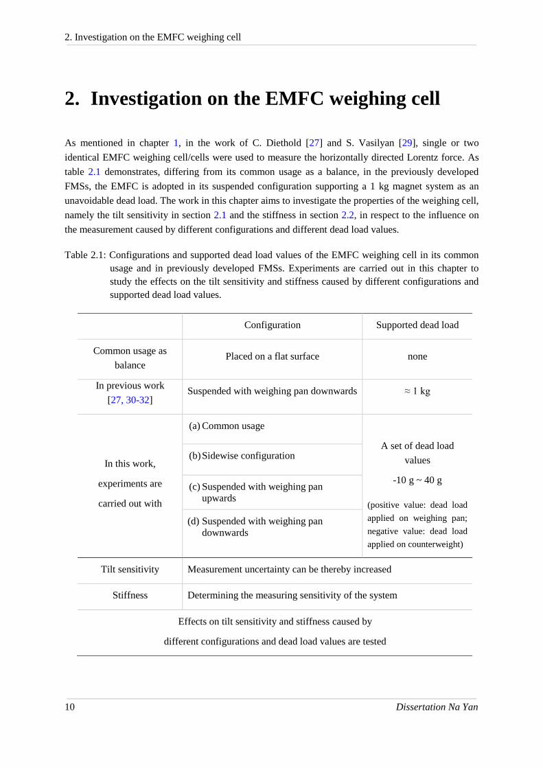
As mentioned in chapter 1, in the work of C. Diethold [27] and S. Vasilyan [29], single or two
identical EMFC weighing cell/cells were used to measure the horizontally directed Lorentz force. As
table 2.1 demonstrates, differing from its common usage as a balance, in the previously developed
FMSs, the EMFC is adopted in its suspended configuration supporting a 1 kg magnet system as an
unavoidable dead load. The work in this chapter aims to investigate the properties of the weighing cell,
namely the tilt sensitivity in section 2.1 and the stiffness in section 2.2, in respect to the influence on
the measurement caused by different configurations and different dead load values.
Table 2.1: Configurations and supported dead load values of the EMFC weighing cell in its common
usage and in previously developed FMSs. Experiments are carried out in this chapter to
study the effects on the tilt sensitivity and stiffness caused by different configurations and
supported dead load values.
Configuration Supported dead load
Common usage as
balance Placed on a flat surface none
In previous work
[27, 30-32] Suspended with weighing pan downwards ≈ 1 kg
In this work,
experiments are
carried out with
(a) Common usage
A set of dead load
values
-10 g ~ 40 g
(positive value: dead load
applied on weighing pan;
negative value: dead load
applied on counterweight)
(b) Sidewise configuration
(c) Suspended with weighing pan
upwards
(d) Suspended with weighing pan
downwards
Tilt sensitivity Measurement uncertainty can be thereby increased
Stiffness Determining the measuring sensitivity of the system
Effects on tilt sensitivity and stiffness caused by
different configurations and dead load values are tested

2. Investigation on the EMFC weighing cell
Dissertation Na Yan 11
2.1 Tilt sensitivity of the EMFC weighing cell
In comparison with the system using single EMFC weighing cell, by using a second identical
weighing cell in the DFMS, the force resolution is improved from 1 µN to 20 nN by factor 50. This
improvement is achieved by using a reference system to measure and compensate the errors caused by
thermal drift/tilt and seismic noises which play a significant role in the small force measurement. In
order to improve the force resolution, these errors are expected to be further investigated. The
tilt/movement of the foundation, on which a FMS is placed, is a summation of factors caused by
human activities, motion of machines nearby and the seismic activities of the earth, including earth
tides [33]. Moreover, the thermal deformation of support frames leads to the tilt of the FMS. As an
obvious outcome of the influences of tilt on the measurement, the tilt sensitivity of the EMFC
weighing cell is discussed in this section.
Figure 2.1: The EMFC weighing cell in its suspended configuration: a) In perfectly vertical aligned
direction; b) Misaligned with a tilt angle α. The green block indicates the deadweight at
the position of the weighing pan m1 with arm length L1; yellow block indicates the
deadweight on the other side of the pivot m2 with arm length L2. Positioning sensor gives
voltage U(t) to PID controller and current Ic is applied on the coil for the compensation
procedure.
The EMFC weighing cell can be simply sketched as a lever arm with the deadweight at the position of
the weighing pan m1 on one side and m2 as the counterweight on the other side [34]. In order to
measure horizontally directed forces, the EMFC was configured in its suspended position in [27] and
[29] as presented in figure 1.4. For an ideal case illustrated in figure 2.1 (a), external force FL' acts on
the weighing pan causing the deflection of the lever arm, which is detected by the positioning sensor
giving the continuously measured voltage U(t). Based on a PID-controller, compensation current Ic
can be calculated concerning the lever's deflection and be transferred to the voice coil integrated in the
weighing cell. With interaction between the coil and magnet, compensation force Fc is generated
g
m2
z
x y
m1
S N
Ic
α
L2
L1
(a) (b)
U(t)controller
Ic
U(t)
controller
S N
FL
Fc
‚

2. Investigation on the EMFC weighing cell
12 Dissertation Na Yan
against the external force and brings the lever arm back to the null position. In this way, the external
force is measured by the compensation force Fc.
However, in real experimental situations, a perfectly aligned vertical configuration as shown in figure
2.1 (a) is difficult to achieve due to the causes of tilt discussed above. Assuming that between the
horizontal plane and the frame of the weighing cell there is a tilt angle α illustrated in figure 2.1 (b), as
a consequence, tilt forces Ft1 and Ft2 caused by deadweight force and the tilt angle will act on m1 and
m2 respectively. Both tilt forces lead to the torque Mt described in equation (2.1):
1 1 sintF m g ; 2 2 sintF m g and 1 1 2 2t t tFM F L L (2.1)
When the parameters of the weighing cell do not fulfill the requirement indicated by equation (2.2),
the torque Mt drives the lever arm to leave its equilibrium. The positioning sensor detects this
displacement, which leads to the change in the output signal, even if no external forces act on the
system. The measured force is thereby distorted.
1 1 2 2sin sin 0tM m g L m g L
Namely, 1 1 2 2m L m L (2.2)
Based on equation (2.1) and (2.2), the error signal caused by torque Mt is proportional to sine of the tilt
angle α and the value of (-m1 · L1 + m2 · L2). Because that the weighing cell aims to measure force acting
upon the weighing pan, the error signal is expressed in the form of force rather than torque. Therefore,
this error signal is described by the tilt force Ft as denoted in equation (2.3).
2 2 1 1
1 1
( ) sintt
M m L m L gF
L L
(2.3)
The relationship between the tilt force Ft and the tilt angle α is the tilt dependency of the system. As
equation (2.3) indicates, the tilt force can be further amplified in the LFV application where the value
of m1 is enlarged by carrying the 1 kg magnet system.
To investigate how the tilt angle influence the measurement of the EMFC weighing cell with different
configurations and dead load values, moreover, with the aim to find a way to minimize the influence
caused by tilt, various experimental tests are carried out with the EMFC weighing cell located on a tilt
stage. The tilt stage introduced in [35] is driven horizontally by two high precision linear motors in
both x-and y-direction, with wedge-form combinations the horizontal movement can be transferred
into vertical movement to actuate tilt angles with a resolution of down to 1 µrad in the range of
± 17.4 mrad. The weighing cell, fixed on the tilt stage using additional mechanical support, can be set
into controllable stepwise tilt. Synchronously, the compensation force maintaining the lever arm at
null position and describing the tilt force Ft is recorded. When the system does not fulfill the
requirement of equation (2.2), according to equation (2.3) the tilt force Ft as the output signal from the
weighing cell should also be in a stepwise form corresponding to the tilt angles. Although the
weighing cell is not designed initially to satisfy equation (2.2) by the manufacturer, this can be

2. Investigation on the EMFC weighing cell
Dissertation Na Yan 13
manually achieved by changing the value of m1 and/or m2, which can be realized by adding mass
pieces on the weighing pan or on the other side of the lever arm. In order to create a full picture of the
tilt sensitivity, the EMFC weighing cell is placed in a set of experiments on the tilt stage in four
different configurations as presented in the figure 2.2. Configuration (a) describes the common usage
of the weighing cell as a balance while configuration (d) demonstrates the usage of the suspended
weighing cell to measure the Lorentz force in previous work [27,29]. Configuration (b) and (c)
indicate the rotation of the weighing cell around x-axis counterclockwise from configuration (d) by 90°
and 180° respectively.
Figure 2.2: Four configurations to locate the EMFC weighing cell on the tilt stage. (a) Common
configuration as a balance; (b) Sidewise configuration; (c) Suspended with weighing pan
upwards, (d) Suspended with weighing pan downwards. (1) Tilt stage; (2) Assembled
mass standard and its carrier; (3) EMFC weighing cell; (4) Mechanical support for fixing
the weighing cell on the tilt stage.
The experiments are carried out as follows:
(1) In each of the four configurations, different dead loads (mass pieces) are assembled to the
EMFC weighing cell to change the value of m1 or m2.
(2) With each dead load value, the tilt sensitivity of the EMFC system is to be determined. The
stepwise tilt angles in the range of ± 8 mrad are generated by the tilt stage around x- and then y-
axis respectively. The resulted output signal is then recorded.
With the aims to:
(1) Determine how the dead load affects the tilt sensitivity; and to find the value of the dead load,
by which the tilt sensitivity is zero, namely, equation (2.2) is achieved.
(2) Determine how the configuration affects the tilt sensitivity.
z
x y
(a) (b)
(c) (d)
(1)
(2)
(3)
(4)

2. Investigation on the EMFC weighing cell
14 Dissertation Na Yan
Experimental data of the measurements in configuration (d) is shown in figure 2.3 as an example.
Each single line describes the dependency of the tilt forces on the tilt angles with each applied dead
load in the range of 0 g to 52 g (in this experiment all the additional dead loads are applied on the
weighing pan). With the same applied mass piece as the dead load, a tilt angle around y-axis leads to a
significant higher output force than that caused by the same tilt angle around x. The monolithic
parallelogram structure with the very fine elliptical notch flexures only enables the weighing cell
rotate by its pivot around y-axis while the rotational freedom around x-axis is restricted. Theoretically,
the system is thereby insensitive to the tilt around x-axis. The measured tilt dependency around x
shown in the left figure of figure 2.3 is a consequence of misalignment, in which the coordinate of the
weighing cell (x'y') is not aligned perfectly to the coordinate of the tilt stage (xy). Although in the
measurements the tilt is controlled by the tilt stage around its x-axis, tilt of the weighing cell still
occurs around its sensitive axis y' when the weighing cell is misaligned from the tilt stage by an angle
of γ as demonstrated in figure 2.4. Thereby the output of the weighing cell is also tilt dependent on the
tilt around the x of the tilt stage. As γ is a minor angle by careful alignment, the measured tilt
dependency around x-axis is much lower than that around y-axis corresponding to the figure 2.3.
Figure 2.3: Tilt dependency of the EMFC weighing cell: output forces against tilt angles around x-axis
(left figure) and around y-axis (right figure) by applying different dead loads. The value of
the dead load presented in the middle is the summation of the mass of applied mass piece
and its carrier.
By comparing the measured data while the tilt stage tilts around its x- and y-axis, the angle of the
misalignment γ can be estimated and correction can be added on the measured data with equation (2.4)
and (2.5):
1 1 2cos sinP P P' (2.4)
2 1 2sin cosP P P' (2.5)
P1 - In the perfectly aligned case (γ = 0), output of the weighing cell with tilt stage tilting around x;

2. Investigation on the EMFC weighing cell
Dissertation Na Yan 15
P2 - In the perfectly aligned case (γ = 0), output of the weighing cell with tilt stage tilting around y;
P1' - In real case when γ ≠ 0, measured output of the weighing cell with tilt stage tilting around x;
P2' - In real case when γ ≠ 0, measured output of the weighing cell with tilt stage tilting around y.
As described above, due to its mechanical structure, the weighing cell is insensitive to the tilt around
x-axis when γ = 0, thereby value P1 is zero and the equation (2.4) and (2.5) can be simplified as
equation (2.6). The misalignment angle γ can be calculated with the measured data in the real case,
thus γ is calculated as 0.5270 ± 0.0065° (confidence level k = 2), by which the measured output P1' and
P2' are corrected due to equation (2.6) to determine the theoretical output P1 and P2 in perfectly
aligned case.
1 2 sinP P' ; 2 2 cosP P' ; 1
2
tanP
P
'
' (2.6)
Figure 2.4: Drawing of assembling the weighing cell on the tilt stage with a misalignment angle γ,
corresponding to configuration (d) from top view.
In figure 2.3, the slopes of the lines indicate the tilt sensitivity of the weighing cell and change along
with the different dead load values. With each dead load, the tilt sensitivity is calculated with linear
fitting. Figure 2.5 (d) reveals that the tilt sensitivity is proportional to the value of the weight applied
on the weighing cell, which agrees with the equation (2.3). With the help of a linear regression, the
relationship between the applied mass piece m0 (in [g]) and the tilt sensitivity Tsy (in [mN rad-1
]) is
described in the following form for the weighing cell in configuration (d):
010.035 ( 31.13)yTs m
Weight value m0 = (31.13 ± 0.16) g can be ascertained by tilt sensitivity Tsy of zero. From the
experiments and the calculations above, it can be concluded that the tilt sensitivity of the weighing cell
in its suspended configuration can be theoretically minimized to zero by applying the weight of
31.13 g on the weighing pan.
y
x
y
x
γ Tilt stage
Weighing
cell‚
‚

2. Investigation on the EMFC weighing cell
16 Dissertation Na Yan
Figure 2.5: The tilt sensitivity of the EMFC weighing cell around the sensitive axis (y-axis) in four
configurations (corresponding to figure 2.2) along with the applied dead load values (dead
loads are applied on the weighing pan).
The tilt sensitivity of the weighing cell around the sensitive axis (y-axis) of each configuration is
calculated and drawn in figure 2.5. The same measurement procedure is repeated during the other
three configurations, similar results are achieved in configurations (b) and (c) after the correction with
the misalignment angle γ, where the calculated weight m0 is (31.24 ± 0.15) g and (30.98 ± 0.14) g
respectively. A significant deviation appears in the measurements during configuration (a) when the
weighing cell performs as a classic balance. In this configuration, the tilt sensitivity of the system with
no externally applied dead load is a negative value of -14 mN rad-1
deviated from 312 mN rad-1
in the
other three configurations. The required compensating weight m0 to minimize the tilt sensitivity
appears to be a negative value, which means that instead of adding the mass piece on the weighing pan,
the weight should be applied on the other side of the lever arm, namely on the counterweight. To
clarify this deviation, it is important to have a clear picture of the weighing cell in the four
configurations as figure 2.6 shows, in each configuration the weighing cell is presented with a tilt
angle α around y-axis.

2. Investigation on the EMFC weighing cell
Dissertation Na Yan 17
Figure 2.6: Sketched structure of the tilted EMFC weighing cell in four configurations (corresponding
to figure 2.2). Ic - compensation current; Fc - compensation force; s – defection of the
lever detected by positioning sensor. (a), (c) and (d) are from side view while (b) is from
top view.
As mentioned before, the weighing cell in configurations (b) (c) and (d) can be uniformed as only with
different rotation angles in the yz-plane of 90° for configuration (b), 180° for configuration (c) and 0°
for configuration (d). In these three configurations, the tilt forces act upon both sides of the lever are
proportional to sinα as indicated in figure 2.6 and equation (2.3). However, in configuration (a) the tilt
forces depend on cosα as equation (2.7) shows.
1 1 2 2( ) costF m L m L g (2.7)
In this set of experiments, the tilt angle is produced in a small range of ± 8 mrad, with the small-angle
approximation, cosα ≈ 1 - α2/2 while sinα ≈ α. Thereby, the tilt sensitivity of the weighing cell in
configuration (a) is 1 1 2 2( ) sint
s
dFm L m L g
dT
, is much lower than that in the other three
configurations where the tilt sensitivity is 1 1 2 2( )t
s
dFm L m L g
dT
, and this also explains why
the tilt sensitivity in configuration (a) is negative.
Thus, in this subsection of testing tilt sensitivity, the following results can be concluded:
1) The tilt force Ft depends linearly on the tilt angle around its sensitive axis (y-axis);
m2
m1
Ic
Fc
L2
L1
Ic
Fc
m2
m1
m2
Ic
m1
s
g
g
x
y z.
g
z
x y
m1∙ g ∙ sinα
m2∙ g ∙ sinα
m1∙ g ∙ sinα
m2∙ g ∙ sinα
(b)(a)
(d)(c)
.
z
x y.
Fc
m1∙ g ∙ sinα m2∙ g ∙ sinα m2
m1
α
m1∙ g ∙ cosα
m2 ∙ g ∙ cosα
Ic
g
z
x y.
α
α
α S N
Fc

2. Investigation on the EMFC weighing cell
18 Dissertation Na Yan
2) The tilt sensitivity is linearly dependent on the dead load added on the weighing cell. In
configurations (b) (c) and (d) similar results are achieved while the result in configuration (a)
differs from the other three. The cause is explained by figure 2.6. By supporting the 1 kg
magnet to measure the Lorentz force, the tilt sensitivity can be further amplified and the
measurement uncertainty can thereby increase;
3) Due to the theoretical calculation and experimental results, the tilt sensitivity can be
minimized to zero by adding the appropriate dead load on the weighing cell, namely by
fulfilling the requirement of equation (2.2).
2.2 Stiffness of the EMFC weighing cell
Stiffness of a FMS describes the ratio between the force and the resulted displacement. High stiffness
indicates robust FMSs, while low stiffness means the higher sensitivity to detect lower forces. The
stiffness is also an important index that defines the resolution of the force measurement. With the
same technique of positioning detection, a FMS with lower stiffness indicates that it can resolve lower
forces. Similar to the investigation on the tilt sensitivity with a set of dead loads, how the dead loads
affect the stiffness of the weighing cell is also expected to be studied with the four configurations.
Figure 2.7: Block diagram of compensation procedure of the weighing cell and an option to test the
stiffness (in red dash block).
Considering the working principle of the EMFC weighing cell demonstrated in figure 2.7, the position
change of the lever caused by forces is continuously recorded and described by the output voltage U(t)
of the positioning sensor. The error signal e(t) as the difference between the measured voltage U(t) and
the defined voltage value U0 is transferred to the servo-controller. Compensation current Ic is
calculated and applied to the voice coil actuator to generate the compensation force Fc, which brings
the lever back to the null position. Alternatively, in the open-loop operation mode where the PID
servo-controller is not used, by using the voice coil as a force actuator, controllable stepwise current Ia
is applied to the coil to generate controllable stepwise actuation forces Fa. This force leads to the
deflections of the lever arm s detected by the positioning sensor and described by the output voltage U.
In this way, the stiffness of the weighing cell Cs can be experimentally determined as equation (2.8)
shows, where c1 is a constant depends on the properties of positioning sensor and voice coil.
1a a
s
F IC c
s U (2.8)
Levere(t)
PIDIc Voice
coil
Fc UU0
Measurements
-
U(t)
Test for stiffness
Ia Fa s

2. Investigation on the EMFC weighing cell
Dissertation Na Yan 19
As shown in figure 2.8, the lever arm is driven by the actuation force Fa and rotates to a new
equilibrium as a summation effect of the forces including: ① the electromagnetic actuation force Fa;
② components of the gravity forces caused by mass m, gravitational acceleration g and angular
deflection β; and ③ the elastic force caused by the spring constant of the mechanical structure Cp and
the angular defection of the lever arm β.
Figure 2.8: Sketched of the main structure of the EMFC weighing cell together with the parameters
used to determine the stiffness of the system, in four configurations (corresponding to
figure 2.2). (a), (c) and (d) are from side view while (b) is from top view.
Following are the variables presented in figure 2.8 and adopted in later calculations:
Fa [N] Electromagnetic actuation force leading to deflection of the lever
Lm [m] Arm length of the actuation force Fa, distance from the voice coil actuator to
the pivot
m1 [kg] Deadweight at the position of the weighing pan on one side of the lever
m2 [kg] Deadweight of the counterweight on the other side of the lever
∆m1 [kg] Additionally applied mass on the weighing pan
∆m2 [kg] Additionally applied mass on the counterweight
L1 [m] Arm length of the deadweight m1
m2
m1
Fa
L1
L2
s
Ia
s
Fa
m2
m1
m2
m1
Ia
m2
Ia
m1
s s
g
g
z
x y
g
x
y z.
g
z
x y
m1∙ g ∙ sinβ
m2∙ g ∙ sinβ
m1∙ g ∙ sinβ
m2∙ g ∙ sinβ
m1∙ g ∙ cosβ
m2∙ g ∙ cosβ
(b)(a)
(d)(c)
.
.
z
x y.
Fa
m1∙ g
m2∙ g
β β
β
β
Ms
Ms
Ms
Ms
Lm
Ls
Fa
L1 L2
Lm
Ls
Lm
Ls
L1
L2
Lm
Ls
S N
S N
S
N
Ia
S
N

2. Investigation on the EMFC weighing cell
20 Dissertation Na Yan
L2 [m] Arm length of the dead weight m2
β [rad] Angular defection of the lever arm, caused by actuation force Fa
Ms [N m] Torque caused by the spring constant of the weighing cell and the angular
deflection β
s [m] Linear displacement at the positioning sensor
Ls [m] Distance between the pivot and positioning sensor
Cs [N m-1
] Linear stiffness of the weighing cell
Cr [N rad-1
] Rotational stiffness of the weighing cell
Cp [N m rad-1
] Spring constant of the mechanical structure of the weighing cell
In each configuration, the linear defection s and linear stiffness Cs can be described by the angular
defection β (β is minor) and rotational stiffness Cr as:
as
FC
s ; a
r
FC
; ss L
Therefore, rs
s
CC
L (2.9)
The torque Ms caused by the spring constant of the lever Cp and the angular deflection β can be
described as:
s pM C (2.10)
Stepwise current Ia is applied to the voice coil while the deflection of the lever is recorded by the
positioning sensor. The tests are repeated with a set of different mass pieces ∆m1 applied on the
weighing pan changing the value of m1; conditionally restricted dead loads ∆m2 are applied on the
other side of the lever arm for changing the value of m2 only with configuration (a). According to
figure 2.8, the analytical calculations for each configuration are as following:
Configuration (a):
When the weighing cell is located in configuration (a) with the common use as a balance, the equation
(2.11) can be written to describe its equilibrium indicated in figure 2.8 (a), where the lever arm is
differed from its null position by the actuation force Fa:
1 1 1 2 2 2( ) cos ( cos 0)a m sF L m m g L m m g L M (2.11)
Together with equation (2.9) and (2.10):

2. Investigation on the EMFC weighing cell
Dissertation Na Yan 21
2 2 2 1 1 1)[( ( ) ] sinpar
m
C m m L m L gdFC
d L
m
1 1 1 2 2 2[( ) ( ) ] sinpr
s
s m s
C m m L m m L gCC
L L L
(2.12)
In case ∆m1 = ∆m2 = 0: 1 1 2 2
0
( ) sinp
s
m s
C m L m L gC
L L
(2.12')
Here the m1, m2, Cp, L1, L2, Lm and Ls are constants that depend on the mechanical structure of the
weighing cell. To investigate the effect of dead load on the stiffness of the system, the added dead
loads ∆m1 and ∆m2 are considered as the variable.
The initial stiffness of the system without additionally applied mass pieces is indicated in equation
(2.12'). The form of the stiffness is complicated as it depends on the angular deflection β, which is not
a constant. However, due to the mechanical structure of the weighing cell, the deflection range of the
lever arm is minor in the range of sub-milliradians; thereby the influence on the stiffness caused by the
change of the angle β is negligible. Thus, by increasing the value m1, the stiffness of the weighing cell
increases while by increasing m2, the stiffness decreases, which matches with the experimental results
demonstrated in figure 2.9 (a). The positive values of ∆m in figure 2.9 indicate the mass pieces are
applied on the weighing pan, while the negative values indicate the mass pieces are added on the
counterweight. In figure 2.9 (a), obvious difference is between the slopes in the two cases where the
additional dead load is applied on each side of the lever arm. As equation (2.12) presents, this is
caused by the difference between the value of L1 and L2 as they are the multiplication factors of the
change in dead load value.
Configuration (b):
In figure 2.8 (b), the weighing cell is located in the sidewise position and is demonstrated from the top
view. The lever deflects around the pivot in the xy-plane as a result of actuation force Fa and the
torque Ms. The gravity forces of m1 and m2 are in the yz-plane and makes no influence on the rotation
of the lever when no tilt exists. Therefore, the equilibrium of the weighing cell can be described with
equation (2.13) and the stiffness of the weighing cell in this configuration can be described as equation
(2.14):
0a m sF L M (2.13)
par
m
CdFC
d L
prs
s m s
CCC
L L L
(2.14)

2. Investigation on the EMFC weighing cell
22 Dissertation Na Yan
Figure 2.9 (b) shows the experimentally obtained stiffness values during the sidewise configuration. In
comparison with the other three configurations, the stiffness does not show significant change along
with the applied dead load values. This also agrees with the analytical calculated equation (2.14)
where deadweight forces make no influences. The deviations in the measured data can be caused by
tilt of the system during the measurements, which leads to distorted output as it was discussed in the
section 2.1.
Configuration (c):
In the suspended configuration with the weighing pan upwards (similar to inverse pendulum) shown in
figure 2.8 (c), the equilibrium of the weighing cell can be described with equation (2.15), by which the
stiffness in this configuration is indicated with equation (2.16):
1 1 1 2 2 2( ) sin ( sin 0)a m sF L m m g L m m g L M (2.15)
1 21 1 2 2( () ) par
m
m m g L m m g L CdFC
d L
with sin
1 21 1 2 2( () ) pr
s
s m s
m m g L m m g L CCC
L L L
(2.16)
In case ∆m1 = ∆m2 = 0: 1 1 2 2
0
( )p
s
m s
C m L m LC
L L
g
(2.16')
Configuration (d):
Similar to configuration (c), in configuration (d) the weighing cell is suspended, however now with the
weighing pan downwards as used previously in [27, 29] to measure the Lorentz force:
1 1 1 2 2 2( ) sin ( sin 0)a m sF L m m g L m m g L M (2.17)
1 21 1 2 2( () ) par
m
m m g L m m g L CdFC
d L
with sin
1 21 1 2 2( () ) prs
s m s
m m g L m m g L CCC
L L L
(2.18)
In case ∆m1 = ∆m2 = 0: 1 1 2 2
0
( )p
s
m s
C m L m LC
L L
g
(2.18')
From the theoretically calculated equations (2.16) and (2.18), it is revealed that in configuration (c) the
stiffness is proportional to the value of -∆m1 while in configuration (d) the stiffness is proportional to
∆m1. Hence, in figure 2.9 (c) the stiffness decreases with the increased dead load on the weighing pan

2. Investigation on the EMFC weighing cell
Dissertation Na Yan 23
while in (d) the situation is opposite. Moreover, when ∆ m1 and ∆ m2 equal to zero which indicates that
no additional dead load is applied, the initial stiffness Cs0 is described by equation (2.16') and (2.18')
for the two configurations respectively. As m1 ·L1 ≠ m2 ·L2, the values of initial stiffness differ from
each other in the two configurations. This also matches with the experiments when no dead load is
applied, the stiffness of the system in configuration (c) is 45.82 N m-1
, which is 41.4% higher than
32.4 N m-1
determined in the configuration (d). This reveals m1 · L1 < m2 · L2, and considering equation
(2.12') and (2.14) this also explains the reason why the initial stiffness Cs0 determined in configuration
(a) is lower than that in configuration (b) with the m1 ·L1 - m2 ·L2 < 0.
Figure 2.9: The stiffness of the EMFC weighing cell in four configurations (corresponding to figure
2.2) along with applied dead loads (positive dead load values mean mass standards are
added on weighing pan changing m1, while negative values indicate dead loads are added
on the counterweight for changing m2).
Thus, in this subsection of testing the stiffness the following results can be concluded:
1) The stiffness of the system can be changed by locating the EMFC weighing cell in different
configurations;
2) By adding dead loads on the EMFC weighing cell, different effects can be acted on changing
the value of stiffness in different configuration as summarized by table 2.2:
a) In configuration (a), adding dead load on m1 increases the stiffness while adding dead load
on m2 the stiffness is reduced;
1.63 N m-1
0.41 N m-1
0.06 N m-1
-0.71 N m-1
0.84 N m-1

2. Investigation on the EMFC weighing cell
24 Dissertation Na Yan
b) In configuration (b), stiffness is constant (not considering the influence caused by tilt);
c) In configuration (c), adding dead load on m1 decreases the stiffness while adding dead load
on m2 the stiffness is increased;
d) In configuration (d), opposite to the case in configuration (c), adding dead load on m1
increases the stiffness while adding dead load on m2 the stiffness is decreased.
Table 2.2: Effects on stiffness caused by different dead load values in four configurations.
Configuration Stiffness
of the system
Common usage as a balance m1 ↑ ↑
m2 ↑ ↓
Sidewise m1 ↑ ─
m2 ↑ ─
Suspended with weighing pan upwards m1 ↑ ↓
m2 ↑ ↑
Suspended with weighing pan downwards m1 ↑ ↑
m2 ↑ ↓
This also indicates that by carrying the 1 kg magnet system in the suspended configuration (d) in
previous researches in [27] and [29], the stiffness of the EMFC weighing cell is thereby largely
increased to 53.92 N m-1
according to the calculation with the linear fitting. This change in stiffness
also leads to the undesired negative effect on measuring sensitivity. As the EMFC weighing cell can
also measure the horizontally directed forces in configurations (b) and (c), it is preferable to arrange
the EMFC in these two configurations carrying the magnet system, because in configuration (b) the
stiffness is constant around 39.42 N m-1
, while in configuration (c) the lower stiffness of 27.76 N m-1
is achieved due to the 1 kg dead load, which makes the system more sensitive.
2.3 Summary
As an essential part in most of the FMSs developed for the LFV, the EMFC weighing cell provides a
better robustness than the PFMS and is expected to measure the force down to nanonewton range.
Differs from its common usage as a balance, the EMFC weighing cell was adopted within the
framework of LFV in its suspended configuration, supporting the magnet system as a dead load over
1 kg. With the aim to study how the configuration and dead load influence the measurement of the
EMFC weighing cell, several experiments were carried out in respect to testing the tilt sensitivity and
the stiffness with four different configurations and a set of different dead load values.
The results of the experiments were concluded above at the end of each subsection. To emphasize,
when using the EMFC weighing cell, it must be noticed that by supporting the magnet system with a

2. Investigation on the EMFC weighing cell
Dissertation Na Yan 25
suspended configuration, the tilt sensitivity of the system can be amplified leading to higher measure-
ment uncertainty. Moreover, the stiffness of the EMFC weighing cell is proportional to the dead load
in the suspended configuration. The 1 kg magnet system also amplifies the stiffness and makes the
system less sensitive.
In the experiments of testing tilt sensitivity, a way was found to eliminate the tilt sensitivity by
applying compensation dead load on the EMFC weighing cell, which can be considered as a way to
reduce the errors caused by unavoidable tilt. However, concerning that in the LFV application, the
EMFC is required to support the 1 kg magnet as the dead load; to compensate this weight on the
precise mechanical structure of the weighing cell is not generally desirable. Using two identical EMFC
weighing cells in the DFMS is an alternative method to reduce the noises Ferr from the FL' (see figure
1.4). In DFMS, it is required to arrange the highly precise geometrical alignment of the two EMFC
weighing cells on the frame. Moreover, the cost of using two highly precise EMFC weighing cells
should also be considered. Therefore, considering the requirement of a tilt-insensitive system
described in equation (2.2), and also with a constant stiffness unchangeable with the supported dead
load values, a torsion force measurement system (TFMS) based on the principle of torsion balance is
developed and introduced in the following chapters. With the TFMS, the force resolution is expected
to be improved by one order of magnitude, namely, from 20 nN (as using the DFMS) to 2 nN.

3. Design concept of torsion force measurement system
26 Dissertation Na Yan
3. Design concept of torsion force measurement
system
The concept of torsion balance is well known as the experiment was carried out by Henry Cavendish
in 1798 to measure the gravitational force between two masses [36]. Nowadays, the principle of
torsion balance is still widely used for highly resolved force measurements as introduced in section
1.2.1. In this chapter, the force measurement system based on the principle of torsion balance, namely
the torsion force measurement system (TFMS), is introduced. In section 3.1, based on the theoretical
calculation considering the resolution of the positioning senor and the expected force resolution, the
geometry of the TFMS is set and the type of commercial bearing is chosen to achieve the appropriate
stiffness of the system. From section 3.2 to section 3.5, the components of the TFMS are introduced in
details.
3.1 Initial idea and theoretical calculation
As indicated in section 1.2.2, the robust EMFC weighing cell is a reasonable replacement of the PFMS
to contribute into Lorentz force measurement. By arranging the weighing cell in the suspended
downwards position depicted in figure 2.2(d), the weighing cell can measure the small horizontally
directed forces with high dead load. In chapter 2, it is revealed that when the mechanical structure of
the measurement system does not fulfill the requirement indicated by equation (2.2), errors can occur
in the measured signal when the measurement system tilts. The tilt can happen with movement of
people, machines or earth crust; as a result, it is unavoidable. Due to the mechanical structure of the
EMFC weighing cell, by adding mass pieces on the weighing pan or on the counterweight, namely
changing the value of m1 and m2, the equation (2.2) can be theoretically achieved to minimize the
influence of the tilt. However, considering the necessity of supporting the 1 kg magnet system while
using EMFC to measure the Lorentz force, it is undesirable to compensate this weight by adding
additional mass piece in such order of magnitude on the precise monolithic structure. Moreover, the
stiffness that defines the measurement sensitivity of the EMFC weighing cell is also further increased
by supporting the dead load in its suspended configuration with weighing pan downwards, in which
case the force resolution is also thereby impaired.
The initial idea of this work is to overcome the difficulty in achieving equation (2.2) by developing a
symmetrical system, where m1 equals to m2 while L1 equals to L2, in another word, center of gravity
(COG) is identical with pivot point (PP). This kind of system is well known as torsion balance, by
which the Cavendish experiment [36] was carried out in 1798 to measure the gravitational force
between large and small spheres. Nowadays, the principle of torsion balance is still widely used to
determine the Newtonian constant of gravitation [21] and to test small weak equivalence principle [23].
Force measurement setups based on the principle of torsion balance differ in every application.
However, the core structure remains the same. Initially in [36], the torsion balance consists of a rod

3. Design concept of torsion force measurement system
Dissertation Na Yan 27
and a thin fiber suspending the rod in the middle. At each end of the rod is a small sphere, and next to
each small sphere located a large sphere on a separated support. Exerting the gravitational force upon
the small spheres, the rod starts to rotate while the fiber twists itself until it reaches an angle, where the
twisting force of the wire balances the gravitational force. According to Hooke's law, the gravitational
force is proportional to the rotational angle and the spring constant of the torsion balance. The spring
constant is determined by measuring the resonant vibration period while the rotational angle is
detected by microscope, the gravitational force is thereby measured.
The mechanical structure of the torsion balance can also be considered as a transformation from the
monolithic mechanical structure of the EMFC weighing cell in its sidewise configuration by
modifying the parameters m1, m2, L1 and L2. Compared with the configuration (c) and (d) in figure 2.2,
in the sidewise configuration, the dead load has a minimized influence on the stiffness of the system.
Therefore, by using the principle of the torsion balance, influences on the measurement caused by tilt
sensitivity as well as change in stiffness can be theoretically overcome.
In order to develop a robust force measurement system which is more appropriate for LFV, the torsion
force measurement system (TFMS) illustrated in figure 3.1 as transformation from the initial torsion
balance, is introduced. Compared to the master setups such as in work [21], where measurements are
carried out with high precision devices under high precision laboratory conditions, the TFMS is
designed with more compact dimensions and with normally achievable components. Sufficient
resolution is achieved under the normal laboratory conditions.
Figure 3.1: Torsion force measurement system: (a) Sketch with flow channel; (b) Snapshot. (1) Flow
channel; (2) Integrated magnet system; (3) Positioning sensor; (4) Plane wheel; (5) Non-
magnetic copper dummy as counterweight; (6) Baseplate; (7) Commercial flexible bearing
hinge; (8a) Outer conical coupling element; (8b) Inner conical coupling element; (9)
Adjustable feet; (10) Mechanical connector; (11) Safety fixture; (12) Replacement dummy
weight; (13) Knurled screw (4 pieces) to lift the plane wheel.
The plane wheel (4) in figure 3.1 carries the magnet system (2) on one side with the arm length LT2,
and on the other side is the non-magnetic dummy weight (5) as the counterweight with the arm length
LT1. When the geometry is perfectly symmetrical, namely LT2 = LT1, and the mass of the dummy is
(1)
(2)(3)
(4)
(5)(6)
(7)
LT1
LT2
(8a)
100 mm
(9)
a)
y
z
x
R
x
y(12)
b)
(10)
(11)
(8b)
(13)FL
θ M
s
(3)
‚

3. Design concept of torsion force measurement system
28 Dissertation Na Yan
identical with the mass of the magnet system, the tilt-insensitive system is thereby achieved by using
this design as the requirement of equation (2.2) is fulfilled.
The reaction force FL' of the Lorentz force induced by the flowing electrolyte in channel (1) acts upon
the magnet system, leads to the torque M and drives the plane wheel rotate with angle θ, which can be
described with equation (3.1).
' T2 L
M L F (3.1)
During rotation of the wheel, the commercial flexible bearing (7) assembled together with the wheel,
is deformed and provides the elastic force balancing the external force. The wheel then gets its new
equilibrium. The deflection of the wheel θ proportional to the torque M is detected by the positioning
sensor (3).
bM C (3.2)
Cb [N m rad-1
] Spring constant of the commercial bearing
A universal principle of measuring force is measuring the deflection of the mechanism with certain
stiffness. As aim of this work is measuring the Lorentz force, the effective stiffness Ct of the TFMS,
corresponding to arm length LT2, is desired to be determined. The rotational angle θ can be transferred
into displacement s at the positioning sensor with s = R · θ (see figure 3.1). Therefore, the effective
stiffness Ct expressing the sensitivity to measure Lorentz force, can be calculated with the geometrical
parameters and the spring constant of the bearing hinge Cb by equation (3.3):
2
bt
T
CC
L R
(3.3)
LT2 [mm] Arm length of the reaction force of Lorentz force
R [mm] Length from the positioning sensor to the center of the TFMS
Considering the expected force resolution of 2 nN and the position resolution provided by the
positioning sensor of 1 nm, the stiffness of the TFMS is expected to be lower than 2 N m-1
. This can be
achieved by modifying the parameters on the right side of equation (3.3). Equation (3.3) indicates that
the stiffness of the system can be decreased by using bearing hinges with lower spring constants or by
increasing the diameter of the wheel, in which cases the maximum axial load of the bearing and the
deformation of the system should also be considered. Thereby, the flexible bearing with the spring
constant of 1.17·10-2
N m rad-1
is chosen with the maximum axial load of 101 N, which is sufficient to
carry the dummy weight and the magnet system. The outer diameter of the wheel is designed as
250 mm, leading to the value of R and LT2 135 mm and 180 mm respectively. The stiffness of the
TFMS is calculated using the equation (3.3) as 0.48 N m-1
and the theoretical force resolution of

3. Design concept of torsion force measurement system
Dissertation Na Yan 29
0.48 nN is expected. The undamped natural frequency of the system fn can be calculated with equation
(3.4):
1
2
bn
Cf
J = 0.06 Hz (3.4)
Here, J is the moment of inertia around the z-axis, and the value of 0.0815 kg·m2 is calculated using
the numerical simulation results. The low undamped natural frequency is a result of the high dead load
as well as the low spring constant of the bearing. Due to the theoretical calculation, the TFMS with an
undamped natural frequency of 0.06 Hz is expected to measure forces down to 0.48 nN. The
components of the TFMS presented in figure 3.1 are introduced in the following sections in details.
3.2 Plane wheel with dead load
In Cavendish experiment [36], the rod carries two identical small spheres at each end. The mutual
attraction force between the small sphere and the leaden large sphere located nearby enables the
twisting of the fiber and rotating of the rod. Analogous situation is for the TFMS to measure Lorentz
force, where the TFMS has to carry the magnet system of over 1 kg to generate magnetic field, upon
which exerted force is to be measured. As a transformation from the rod carrying two spheres in the
initial torsion balance, a plane wheel with the outer diameter of 250 mm ((4) in figure 3.1) is chosen to
carry the magnet system (2) on one side, and on the other side is a the non-magnetic dummy weight (5)
as the counterweight with similar mass and geometrical dimensions. The plane wheel is in
symmetrical geometry with the theoretically equal arm lengths LT1 and LT2, and provides sufficient
place for further assembling. Moreover, the weight is reduced compared to a form of disc with same
diameter and material. The two additional connectors (10) provide the convenience to assemble the
magnet and dummy weight on the plane wheel, and extends the effective arm length LT1 and LT2 from
125 mm to 180 (± 2) mm in order to reduce the stiffness and increase the sensitivity of the system. In
the initial tests of the capabilities of the TFMS, the magnet system is replaced by a second identical
dummy weight (12) to avoid the magnetic interaction caused by the magnet system and other magnetic
material/parts in the laboratory. Therefore, the TFMS with the plane wheel carrying dead load
theoretically meets the requirement in equation (2.2), which describes an insensitive system to
unavoidable tilt.
3.3 Flexible bearing support
3.3.1 Flexible bearing hinge
In [36], the rod and the two small spheres are suspended with a thin fiber, which is connected to the
frame and provides twisting force during rotating to balance the gravitational force. Considering the
TFMS developed for LFV, using the thin fiber and frame is neither space-saving nor constraints the
rotation within the horizontal plane well. A replacement of the thin fiber is desired to build a more
robust and compact system. In the mechanical structure of the EMFC weighing cell, the force is
transformed into deflection by manufacturing monolithic flexure with elliptical notch flexure pivot.

3. Design concept of torsion force measurement system
30 Dissertation Na Yan
Similarly, this kind of precise mechanical structure generating elastic force by deformation can be
used in the TFMS. A reasonable option is using the flexible bearing hinge depicted in figure 3.2,
which is commercially achievable.
The commercial flexible bearing hinge provided by C-Flex Bearing [37] consists of three parts: the
core containing the flexure spring, which deforms and provides elastic force with relative movements
between the two semi-cylinder segments; and two sleeves assembled solidly on each segment of the
core. The sleeves and the core are so assembled coaxially that sleeve 1 is fixed on the core with
segment 1, while untouched with segment 2. Analogously, sleeve 2 is fixed on segment 2 but
separated from segment 1. The assembled areas are highlighted on the sleeves with pink color. As the
side view and top view present, the load acting on sleeve 1 is transferred onto segment 1 assembled to
it, while the other segment together with sleeve 2 is fixed. This leads to the deformation of the flexure
springs and generates the twist; the elastic force thereby balances the external load. In this way, the
commercial flexible bearing enables the rotational motion without friction; similar to the fiber
contributes to the torsion balance. An advantage of using the commercial flexible bearing is that the
bearings are provided by the manufacturer with different specifications (dimensions and values of
spring constant), which makes it convenient to achieve multiple sensitivities in force measurement. In
this work, the bearing type D-10 with spring constant 1.17·10-2
N m rad-1
and diameter of 6.35 mm is
chosen based on the theoretical calculation considering the aim resolution of 2 nN. The maximum
permissible rotational angle provided by the chosen bearing is ± 15°, which is sufficient for the TFMS
to measure force in sub-micronewton range.
Figure 3.2: Mechanical structure of commercial flexible bearing hinge, drawn according to the data
provided by the manufacturer [37].
3.3.2 Conical coupling
The mechanical components shown in figure 3.1 are manufactured from aluminum AW 7075 alloy.
The plane wheel and the additional connectors together with the two copper dummy weights are
approximately 3 kg, not exceeding the maximum axial load value of the bearing, given by the
Sleeve 1
Sleeve 2
Core
Fixed
Load bearingFlexure
spring
Top view
Side view
Fixed
Load
Semi-cylinder
segment 1
Semi-cylinder
segment 2
d = 6.35 mm

3. Design concept of torsion force measurement system
Dissertation Na Yan 31
manufacturer as 101 N. In reality during assembling, imperfection in alignment can exist. Moreover,
during storage or usage, undesired vibrations of ground may occur. In these cases, radial loading in
compression and tension can also exist and damage the bearing. To overcome this problem, the
additional conical coupling elements (8a) and (8b) in figure 3.1 are designed to avoid the damage.
As illustrated in figure 3.1, the conical coupling elements consist of two inner wedges 8(b) and two
outer wedges 8(a). Each inner wedge and outer wedge match with each other by a fine machined 60°
angle without fixing element. The two identical inner wedges are glued on each sleeve of the bearing.
One of the two outer wedges is screwed on the plane wheel while the other one is screwed on the base
plate. Instead of fixing the sleeves of the flexible bearing directly with the plane wheel and the base
plate, using this wedge shaped connection with conical coupling elements provides on one hand the
stable combination of components during measurements under peaceful situations, and on the other
hand enables the relative movement between inner and outer wedges to protect the bearing in
aggressive situations where high amplitude vibration occurs.
3.4 Positioning sensor
In the torsion balances developed nowadays, high resolution devices such as autocollimators and laser
interferometers are widely used for detection of the position. The kind of optical positioning sensor
[38] used in the TFMS ((3) in figure 3.1) is commercial and also used in the EMFC balances to detect
the motion of the lever arm. Compared to autocollimator and interferometer, the optical positioning
sensor provides enough resolution for the measurements in this work with an extremely reduced
compact dimension. The simplified structure of the positioning sensor is illustrated in figure 3.3 (a),
where the infrared-LED (1) as the light source illuminates the two-segment differential photodiode (3)
via a narrow rectangular aperture (2).
Figure 3.3: Structure of the optical positioning sensor. a) Side view. b) Top view, mounted on the
TFMS. (1) LED with metal housing; (2) Aperture; (3) Two-segment differential
photodiode with metal housing; (4) Plane wheel; (5) Base plate.
x
yz
z
yx.
(1)
(2)
(3)
a) b)
(4)
(5)
.

3. Design concept of torsion force measurement system
32 Dissertation Na Yan
Figure 3.3 (b) highlights the positioning senor mounted on the TFMS, where the aperture is fixed on
the plane wheel as the rotational component, and the LED and the photodiode are fixed on the base
plate as the unmovable components. When the aperture moves together with the plane wheel as a
result of external force, the received light on one segment of the photodiode increases while decreases
on the other. The difference of the two signals is proportional to the position change of the aperture
and results in the voltage change as the output signal. This technique of position measurement enables
variable measurement ranges, resolutions and sensitivities by assembling different types of LEDs,
photodiodes and the different sizes of aperture. The optical positioning sensor used in this work
provides a resolution of 1 nm.
As the first test of the optical positioning sensor, the LED illuminates directly on the photodiode
without aperture. Nearby is a thermal resistor, by which the temperature around the positioning sensor
can be changed. The positioning sensor together with the thermal resistor is covered with polystyrene
box for thermal and light isolation. Without considering the object whose position is to be measured,
the LED and photodiode is thermal dependent as indicated in figure 3.4, with the coefficient of
approximately 0.27 mV K-1
. All the experiments with the TFMS are implemented in the laboratory
condition where the temperature is constant within 0.1 K over several days. By this temperature
change, the change in measured voltage value from positioning sensor results to 27 µV, which is taken
in to consideration in the later calculation.
Figure 3.4: Test of the temperature dependency of the positioning sensor (without aperture). Blue:
Output of the positioning sensor during 12 hours; red: controlled temperature change
with a thermal resistor. Inset: output voltage changes along with the temperature.
The voltage being the initial output of the positioning sensor is recorded by a 4-channel-analog input
module NI 9239, providing measurement range of ±10 V at a 24-bit resolution with the maximum
sampling rate of 50 kS s-1
[39]. The NI module is first calibrated with the reference values from a
multi-function calibrator FLUKE 5720A which was calibrated at PTB. Stepwise values in the range of
± 10 V indicating the full measuring range and ± 1 V as the linear output range of the positioning

3. Design concept of torsion force measurement system
Dissertation Na Yan 33
sensor are transferred into the NI module. The measurement uncertainty of each step is determined and
figure is shown in the appendix A. In both ranges, the mean value of the uncertainties at all steps is
9.24 µV. This module provides sufficient measurement capabilities for TFMS with a compact
dimension.
3.5 Adjustment and safety components
The TFMS is located on a granite workbench. The base plate (6) in figure 3.1 is supported on the
workbench by three fine adjustable screws (9) with a pitch of 0.25 mm. With the three-feet-support,
the working plane of the TFMS can be adjusted finely around its x- and y-axis. Two additional screw
feet are assembled to the TFMS without touching the workbench only for safety. The two connectors
(10) are screwed on the plane wheel on one side and support each dummy weight on the other side. By
connection, the tolerance of ± 2 mm is available to provide the possibility to adjust the arm length LT1
and LT2. The safety fixtures (11) limit the rotation of the wheel within a safe working range, which is
enough for measurement in sub-micronewton and not exceeding the rotational angle of ± 15° given by
the manufacturer in case undesired punch or shock occurs. The four knurled screws (13) under the
plane wheel are screwed on the base plate, each of which is further processed so that on the upper
surface a ball is assembled. During the TFMS operates to measure forces, the knurled screws together
with the small balls are separated from the plane wheel. For storage, the knurled screws are firstly
screwed carefully upwards until the balls touch the plane wheel, and then screwed further to lift up the
plane wheel, so that the flexible bearing is free from load and thereby under protection.
3.6 Summary
As a replacement and improvement of the previously used FMSs to measure Lorentz force, the TFMS
based on the principle of torsion balance is introduced in this chapter. A plane wheel together with the
dead loads carried by it is in a symmetrical geometry. The commercial flexible bearing is used to
enable the non-frictional rotational motion and provide elastic force during deformation to balance the
external forces. Various types of bearings with different specifications are commercially achievable
according to various requirements in applications. A state-of-the-art optical positioning sensor is used
to detect rotational angles, which are transferred into force values with stiffness. Theoretically, the
system fulfills the requirement of equation (2.2), which describes an insensitive system to unavoidable
tilt angles. Moreover, with a similar structure as the EMFC weighing cell in its sidewise configuration,
the stiffness of the TFMS remains constant with different values of dead load. Due to geometrical
dimensions and parameters given by the manufacturer, the theoretically calculated force resolution is
0.48 nN with the undamped natural frequency of 0.06 Hz. To achieve a system with force resolution
of 2 nN, the calculated theoretical resolution is acceptable. As a summary, the geometrical and
functional parameters of the TFMS are presented in the table 3.1.
Based on this design concept, various TFMSs with different dimensions and sensitivities can be
manufactured not only for LFV but also for fitting different applications. In addition to the flexibility,
the TFMS is more cost effective, yet has the potential to achieve the expected force resolution in the
range of nanonewton.

3. Design concept of torsion force measurement system
34 Dissertation Na Yan
Table 3.1: Geometrical and functional parameters of the TFMS.
Term Value Unit
Diameter of plane wheel 250 mm
Arm length of dead loads LT1, LT2 (adjustable within ± 2 mm) 180 mm
Arm length of the positioning sensor (adjustable within ± 1 mm) 135 mm
Mass of magnet system 1.008 kg
Mass of dummy 1.071 kg
Mass of rotational components supported by bearing ≈ 3 kg
Max. load capacity of the bearing ≈ 10 kg
Diameter of bearing 6.35 mm
Max. compression 16.02 N
Max. tension 63.19 N
Spring constant of bearing 1.17·10-2
N m rad-1
Resolution of positioning sensor 1 nm
Theoretical effective stiffness 0.48 N m-1
Theoretical force resolution 0.48 nN
Undamped natural frequency 0.06 Hz

4. TFMS in the open-loop operation mode
Dissertation Na Yan 35
4. TFMS in the open-loop operation mode
Based on the design concept introduced in chapter 3, the components of the TFMS are manufactured
and assembled together. In this chapter, adjustments, calibration procedures and experiments are
carried out on the TFMS in the open-loop operation mode. Utilizing the behavior of the TFMS during
tilting, the deflection method is introduced as a traceable method to perform position calibration
(section 4.1) and force calibration (section 4.2). Although the TFMS is introduced as a theoretically
insensitive system to the unavoidable tilt, imperfections in geometry of the mechanical components
and misalignment during assembling can occur in reality. Consequently, the tilt sensitivity is no longer
zero and cannot be ignored. Therefore, similar to that in section 2.1, the test and minimization of the
tilt sensitivity of the TFMS is described briefly in section 4.2.1. In section 4.3, the system
identification of the TFMS in the open-loop operation mode is presented.
4.1 Position calibration using deflection method
As mentioned in section 3.4, the optical positioning sensor detects the movement of the plane wheel
and outputs voltage as the measured signal. In order to detect the position change, the voltage is
expected to be calibrated into rotational angle values. The general procedure for position calibration is
presented in figure 4.1. An autocollimator Elcomat 3000 [40] is chosen as a reference system to
measure rotational angles θ. When the plane wheel is excited by the actuation force Fa into
controllable stepwise rotation motion in the horizontal plane, the motion is detected by the positioning
sensor with the output voltage UP as well as by the autocollimator with the measured rotational angle θ.
The calibration factor Kps can be thereby experimentally determined. Moreover, when the actuation
force Fa is traceable, the force calibration can be implemented by comparing the voltage UP with the
force value, which will be introduced in section 4.2.
Figure 4.1: Block diagram of the calibration process of the positioning sensor using the autocollimator
as the reference system. When the actuation force Fa is traceable, force calibration can be
thereby implemented by comparing the force value with the output voltage UP.
TFMS
Positioning
sensor
Auto
collimator
Fa motion
Voltage UP
Rotational
angle θ
θ = Kps ∙ UP
Fa = KF ∙ UP Force calibration
(section 4.2)

4. TFMS in the open-loop operation mode
36 Dissertation Na Yan
Reproducible actuation forces Fa are usually necessary for executing comparison and calibration
procedures in the force measurement technique. In factory inspection of balances or researching in
weighing instruments, deadweight forces in vertical direction are usually provided by high class
weight-set [12,18]. In applications where horizontally directed actuation forces are desired, for
example, to actuate the TFMS into motion, there are several techniques and commercial products can
be used in the current state. Voice coil actuator can generate electromagnetic actuation forces;
capacitive force actuator can provide electrostatic forces; piezo actuators and micro stages can
generate actuation strokes. Avoiding fixing/screwing voice coil or electrode of capacitor as additional
components on the TFMS where electric current or voltage is necessary to be supplied, reproducible
forces in quasi-horizontal plane can be generated taking convenience of using devices in the laboratory
based on the deflection method.
4.1.1 Force/ motion actuation using deflection method
Based on previous research on the EMFC weighing cell introduced in section 2.1, when the suspended
weighing cell deflects from the gravitational direction by a tilt angle α, a tilt force Ft presented in
equation (2.3) exerts on the system and distorts the measurement result. To reduce the uncertainty of
measurement, the tilt sensitivity of the system is expected to be minimized as introduced in chapter 2.
The precondition for an insensitive system to tilt angles is described by equation (2.2), where the
product of the dead load m1 on one side multiplied by the lever arm L1 equals to the dead load m2 on
the other side multiplied by the lever arm L2. This can be further explained as the pivot point (PP)
being identical to the center of gravity (COG) of a general system.
Figure 4.2: General description of a system, by which COG shifts from the PP as the cause of the tilt
sensitivity.
In a general system, when COG of the system is not identical to the PP but with the shift Lx and Ly as
demonstrated in figure 4.2, the system will leave its equilibrium position driven by the torque Mt when
tilt angles exist, as equation (4.1) denotes:
( sin ) ( sin )x y t x g y gM L F L F , where gF m g (4.1)
COG
Ly Lx
m
yx
z
PP
αy
θ
αx

4. TFMS in the open-loop operation mode
Dissertation Na Yan 37
When the shift Lx, Ly, the tilt angle αx, αy and the mass m are controllable and reproducible, the
outcome torque calculated from equation (4.1) is also reproducible. Force values can be derived from
the torque with known arm length. Thereby, reproducible motion of the TFMS is enabled by using the
deflection caused by tilt angle and shift of COG. Under this condition, the actuation force Fa is
achieved using the deflection method. With the achieved actuation force Fa, the position calibration is
carried out by comparing the output voltage of the positioning sensor UP and the measured rotational
angle θ by autocollimator as indicated in figure 4.1 [41].
4.1.2 Experimental facility
The deflection method is based on the displacement of COG and the tilt of the system, due to which
the tilt force is generated and utilized as the actuation force. The displacement of COG can be
performed by adding standard weight on the system, while the reproducible tilt is enabled by the tilt
stage. In order to implement the position calibration procedure, reproducible motion of the TFMS is
realized using the deflection method by setting up the experimental facility illustrated in figure 4.3.
Figure 4.3: a) Calibration setup using deflection method: (1) Polystyrene box as cover of the system,
inside of which located the TFMS; (2) Autocollimator as reference system; (3) Mirror for
reflecting the beam; (4) Tilt stage to provide tilt angles; (5) Standard weight of class E2
added on the TFMS to cause the shift of COG; b) Simplified drawing from top view; c)
Simplified drawing from side view.
The TFMS is located on the tilt stage (4) and fully covered by a polystyrene box (1) to keep the
airflow out, moreover, for thermal und light isolation. The tilt stage provides the possibility to generate
controllable tilt angle αx and αy around both x- and y-axis. An assumption (a) is made that at the initial
state, the COG of all rotational components (plane wheel, adaptors with dummy weights carried by the
flexible bearing hinge) lies in the rotational axis of the system, namely, no shift of COG exists. By
applying a standard weight (5) on the arm of the TFMS with the arm length r = LT1 (see figure 4.3 a
α
θ
(4)
(2)
(1)
(3)
(5)
. y
x
z
Ft
xy
z
Fg
Ft
α
b)
c)
r
a)
(5)

4. TFMS in the open-loop operation mode
38 Dissertation Na Yan
and b), the COG of the system is thereby displaced. Moreover, when the tilt stage generates a tilt angle
α around y-axis, the tilt force Ft which is proportional to sinα and the mass of the standard weight m is
generated, acting at the point where the standard weight is applied as equation (4.2) denotes. As
illustrated in the simplified drawings (b) and (c) the tilt force Ft operates as the actuation force and
drives the plane wheel into motion.
sina tF F m g (4.2)
A plane mirror (3) mounted on the plane wheel reflects the laser beam back to the autocollimator,
enabling the detection of the tilt angle α and rotational angle θ as figure 4.3 (a) presents. The
calibration factor Kps is determined by comparing the rotational angle θ and the measured voltage UP
from the optical positioning sensor.
The assumption (a) is valid only under the condition that the mechanical components are in even
density, additionally manufactured and assembled ideally symmetrically in geometry. Otherwise, due
to the initial displacement of COG, the tilt force Ft' exerting on the system in reality can be deviated
from the calculated force Ft using equation (4.2). As the displacement of COG caused by the
imperfection during the manufacturing and assembling is an unknown value, the generated tilt force
Ft' in reality is reproducible but not a traceable value. However, for the calibration of the positioning
senor aiming to transfer the electric voltage into rotational angle values as the output signal, generating
the reproducible actuation force driving the wheel into controllable rotation is the focal point. The
exact magnitude of the tilt force is currently not necessary to be under consideration, which means that
the assumption (a) is currently acceptable for the position calibration.
4.1.3 Measurements
In the experiments, standard weight of m = 1 g from class E2 is applied on the TFMS, and the tilt stage
provides the tilt angle αy round y-axis with step of 0.1 mrad in the range of ± 3 mrad. This results into
the rotation of the plane wheel, which is detected by the optical positioning sensor with the output
voltage UP shown in figure 4.4 (a), and by the autocollimator at the same time with rotational angle θ
shown in figure 4.4 (b). As illustrated in figure 4.4 (a), the optical positioning senor presents linearity
only in limited range. The relationship between UP and the θ is presented in figure 4.4 (c), where the
slope of the linear fitting represents the calibration factor Kps. Thus, using this defection method the
calibration factor of the positioning sensor is Kps = (0.4285 ± 0.0015) mrad V-1
with coverage factor
k = 2. The uncertainty is described by repeatability calculated by repeated measurements. Due to the
linear fitting, the residual difference is within 48.99 µrad in the linear range of ± 1.1 V illustrated in
figure 4.4 (d). For the force measurement in this work, a measuring range of ± 20 µN is sufficient to
measure the Lorentz force induced by weakly conducting electrolyte. Therefore, the linear fitting is
implemented within the application range, which is approximately ± 0.6 V shown in figure 4.4 (e). In
this range, the residual difference is considerably better as within 4.05 µrad. The calibration factor is
thereby Kps = (0.4207 ± 0.0012) mrad V-1
and this value is taken in this work according to the local
application.

4. TFMS in the open-loop operation mode
Dissertation Na Yan 39
Figure 4.4: Measured data for position calibration using defection method. (a) Output voltage of the
positioning sensor UP along with tilt angles; (b) Rotational angle θ detected by
autocollimator along with tilt angles; (c) Linear fitting (in linear range) for determining
the calibration factor; (d) Residual difference due to the linear fitting in (c); (e) Linear
fitting (in application range) for determining the calibration factor; (f) Residual difference
due to the linear fitting in (e).
Based on the calibration procedure described in block diagram in figure 4.1, the calibration factor Kps
is determined by the rotational angle θ and measured voltage UP. The autocollimator is with a
4. TFMS in the open-loop operation mode
40 Dissertation Na Yan
resolution of 0.005" [40]. The voltage module NI 9239 with 24 bit resolution [39] is used to record
voltage value, and the measurement uncertainty of it is 9.24 µV (see Appendix A). The value of the tilt
angle α, mass of standard weight m and the arm length LT1 indicating where the weight is applied,
these values are used to enable the motion of the TFMS, however, have no contribution into the
calibration factor Kps. In section 3.4, it was revealed that output of the positioning sensor is
temperature depended, the relative uncertainty of 0.28% in the repeated measurements could be a
summation effect caused by the temperature dependency of the positioning sensor and the
measurement uncertainty of the devices, namely, the NI module and the autocollimator.
4.2 Force calibration using deflection method
In the previous section 4.1, the deflection method is introduced as a reproducible procedure to perform
actuation force on the TFMS, which contributes into the position calibration procedure. Assumption (a)
is made in section 4.1.2 under the condition that during the calibration of the position values, the
reproducible motion of the TFMS is necessary but the exact magnitude of the generated tilt force is
not required. However, the initial displacement of COG of the TFMS caused by imperfection in
manufacture and alignment should be taken into consideration for further investigations, where the
output signal of TFMS is also expected to be calibrated into force values with the aim to measure
Lorentz forces. Therefore, the traceable value of the tilt force is required. Moreover, similar as
measuring with EMFC weighing cell, the tilt sensitivity of the TFMS is desired to be minimized to
reduce the measurement uncertainty. These will be introduced in this section.
4.2.1 Adjustment of the tilt sensitivity
In section 4.1.2, it is assumed that initially, COG of all the rotational components lies in the rotational
axis of the system, in another word, Lx = Ly = 0. This is acceptable when used to calibrate the
positioning sensor from electric voltage into rotational angles. In real cases, the shift of COG does
exist and influences the measurement. However, the shift can be compensated by adding
compensation mass pieces on the system. Although the shift, namely Lx and Ly, are unknown values,
the motion of the TFMS during tilting is the observable outcome of the shift according to equation
(4.1). The compensation of shift of COG is thereby enabled by measuring and adjusting the tilt
sensitivity.
The tilt sensitivity of the TFMS is investigated and adjusted in this section. Similar approach as
described in chapter 2 is carried out with the help of the tilt stage. The TFMS is located on the tilt
stage as illustrated in figure 4.3, but initially without applying any additional standard mass pieces.
Stepwise tilt angles αx and αy within ± 3 mrad are generated respectively, and the rotational angles of
the plane wheel θ are recorded. Ideally the rotational angle θ should remain unchanged with different
tilt angles α when the COG is identical with the PP. However, in the experiment the rotational angle θ
changes linearly with the tilt angle α as figure 4.5 presents. Before any adjustment, the slope of the
line, namely the ratio between the rotational angle θ and the tilt angle αx is Tx1 = -5.6·10−1
indicating
the tilt sensitivity around x-axis; similarly, the tilt sensitivity around y-axis is Ty1 = 2.7·10−1
. Both
values are not zero which indicates that the shift of COG exists in both x- and y-directions, Lx ≠ 0 and
Ly ≠ 0.

4. TFMS in the open-loop operation mode
Dissertation Na Yan 41
Figure 4.5: Tilt dependency of the TFMS before and after adjustment. (Top: tilt angle generated
around the x-axis; bottom: tilt angle generated around the y-axis) and snapshot of the
customized aluminum mass pieces for compensation the displacement of the COG.
With the sign and the magnitude of the obtained tilt sensitivity, the direction of the shift can be
determined and the distance of COG displaced from the PP can be estimated. A set of customized
aluminum components with various dimensions and mass values presented in figure 4.5 are used as
compensation weights, which can be applied and fixed on the plane wheel to compensate the
displacement of COG. Thus, the tilt sensitivity of the TFMS with compensation weight at different
positions is determined until the tilt sensitivity is within the acceptable range. In one work of our
institute [20], the inevitable tilt angle generated by people or environmental factors of approximately
≤ 1 μrad was revealed. The tilt of 1 µrad should not result into a position change of the aperture of
more than 1 nm, which indicates the resolution of the positioning sensor. The calculated limit of tilt
sensitivity is 1 nm μrad−1
, or 7.4·10−3
rad rad−1
(namely 7.4·10−3
) calculated with the distance R of
135 mm (see figure 3.1) from the aperture to the geometrical center of the system. The measurements
and adjustment procedures are repeated until the tilt sensitivity is within the required range. As
demonstrated in figure 4.5 and table 4.1, after the adjustment procedure with the aluminum
compensation weights, the tilt sensitivity is minimized to Tx2 = 4.95·10−5
and Ty2 = -5.5·10−4
, both are
within the permitted range of ≤ 7.4·10−3
.
Table 4.1: Tilt sensitivity of the TFMS before and after the adjustment procedure.
Tilt sensitivity around x around y
Requirement < 7.4·10−3
< 7.4·10−3
Before adjustment Tx1 = -5.6·10−1
Ty1 = 2.7·10−1
After adjustment Tx2 = 4.95·10−5
Ty2 = -5.5·10−4
Tx1 = -5.6 · 10-1
Tx2 = 4.95 · 10-5
Ty1 = 2.7 · 10-1
Ty2 = -5.5 · 10-4
4. TFMS in the open-loop operation mode
42 Dissertation Na Yan
4.2.2 Force calibration
Aiming to measure the Lorentz force, the TFMS should give force values as the output signal. Similar
to that in the section 4.1, where the position calibration is carried out, the deflection method is also
possible to be used for force calibration as indicated in figure 4.1. In the force calibration procedure,
the tilt force Ft generated by defection method should be not only reproducible, but the traceable value
is also required. In order to generate controllable tilt force Ft, a set of defined tilt angles within
specified limits are produced by the tilt stage in the range of several milliradians. Although the tilt
sensitivity was minimized within the permitted range to enable an insensitive system to the
unavoidable tilt angle caused by person or surroundings (≤ 1 µrad), the influences caused by the
remaining tilt sensitivity around both x- and y-axis after the adjustment could not be entirely ignored at
the range of milliradians in the calibration procedure. In this set of measurements, due to the direction
of the Lorentz force in the LFV application, the tilt angles are only necessary to be created around y-
axis. Furthermore, the TFMS is carefully aligned to the axes of the tilt stage to avoid the cross-
sensitivity. Thus, the term sinαx in equation (4.1) could be considered zero. Only the shift of COG
along y-axis (Ly) needs to be considered.
After the adjustment procedure presented in the section 4.2.1, taking in consideration the remaining tilt
sensitivity (also refers remaining displacement of COG), force calibration using the deflection method
is implemented in the following three steps:
i) Without adding known weights
The experimental facility of force calibration is the same as that of position calibration presented in
figure 4.3. Initially, no additional standard weight (component (5) in figure 4.3) is placed on the TFMS.
The tilt stage provides the stepwise tilt angle αy in the range of ± 3 mrad, the motion of the TFMS is
recorded. This motion is a result of the remaining tilt sensitivity Ty2 caused by the remaining
displacement of COG Ly2, which was minimized in the permitted range but still a non-zero value. As
introduced in section 4.1.1, the remaining displacement Ly2 and the tilt angle αy lead to the torque M z*
presented in equation (4.3):
* *
2sinz y yM m g L (4.3)
m* indicates the total mass of the rotational components of TFMS, together with the customized
aluminum compensation weights on the wheel used to adjust the tilt sensitivity. After the adjustment
in section 4.2.1, the value Ly2 is a relatively small but unknown value. However it can be described by
the measured signal. The torque M acting on the system is proportional to the output voltage UP of the
positioning sensor, which can be directly measured by the NI device. The factor Km is introduced as:
m PM K U (4.4)
Therefore, the equation (4.3) can be transferred into equation (4.5).

4. TFMS in the open-loop operation mode
Dissertation Na Yan 43
1
* *
2sinPz y y mM m g L K U (4.5)
Up1 is the voltage change during motion of the TFMS caused by remaining tilt sensitivity, and is
recoded by the NI voltage module.
ii) With additional known weights
In the second step, traceable external force is applied on the TFMS by adding known mass standard m
at a certain position on the wheel with the arm length LT2' along y-axis, this arm length indicates the
position where the force will act in the LFV application. Theoretically, LT2' is equal to LT2 in figure 3.1,
both of which are 180 mm. However, deviation can exist because of the uncertainty of manual
operation. In this work, the maximum permissible error of the positon where the known weight
applied is assumed as 0.5 mm. With the applied known mass standard on the TFMS, the torque Mz
caused by the tilt sensitivity is a summation of two effects: one generated by the remaining shift of
COG after the adjustment procedure; and another by the applied known standard mass piece m.
Similarly, the torque can be described with equation (4.6):
2
*
2 2sin ( )Pz y y T mM g m L m L K U' (4.6)
UP2 is the voltage value from the positioning sensor during the motion caused by tilt.
iii) Difference between step i) and ii)
Subtracting equation (4.5) from equation (4.6), the difference is:
*
2 2 1sindiff z z y T m P m PM M M g m L K U K U' (4.7)
And the introduced factor Km can be calculated as:
2
2 1
sin y T
m
P P
m g LK
U U
'
(4.8)
Since the TFMS is developed to measure force values, the calibration procedure primarily aim to
determine the necessary force calibration factor KF, by which the output voltage of the position sensor
can be converted into forces that act on the magnet system at the effective arm length LT2, equations
(4.9) and (4.10) are shown.
T2M = L ×F ; F PF K U ; m PM K U
and 2
mF
T
KK
L (4.9)

4. TFMS in the open-loop operation mode
44 Dissertation Na Yan
Therefore,
2
2 1 2
sin
( )
y T
F
P P T
m g LK
U U L
'
(4.10)
Each parameter at the right hand side of the equation (4.10) is either known value or measurable. The
force calibration factor KF can be thereby experimentally determined.
The experimental facility used for force calibration remains the same as figure 4.3 presents and the
standard weight of m = 1 g, 2 g and 4 g (as combination of two pieces of 2 g) are added on the TFMS
with the arm length LT2' respectively. With different tilt angle αy and the mass of the standard weight m,
the tilt force Ft is calculated and the corresponding output voltage from the positioning sensor is
recorded and presented in figure 4.6. Linear fitting is applied to the measured data and the slope of the
fitting indicates the factor KF, with which the output of the TFMS can be calibrated into force values.
In figure 4.6, the measured data with different applied standard weights match each other well. The
force calibration factor determined as the mean value of the set of experiments is following with the
uncertainty determined as the repeatability by repeated measurements.
KF = 30.07 ± 0.2 µN V-1
(k = 2)
Figure 4.6: Experimentally measured data to determine force calibration factor KF. (Top: output
voltage along with calculated tilt force in full range of ± 80 µN; Bottom: residual
difference in the application range of ± 20 µN; blue with circle marker: tilt force
generated by mass 1 g; red with cross marker: tilt force generated by mass 2 g; green with
square marker: tilt force generated by 4 g mass piece).

4. TFMS in the open-loop operation mode
Dissertation Na Yan 45
During the rotational motion of the TFMS driven by the tilt force, the rotational angles θ1 in step i) and
θ2 in step ii) are also recorded by the autocollimator. The spring constant of the flexible bearing Cb can
be thereby experimentally determined by equation (4.11):
*
2 1
z zb
M MC
(1.34 ± 0.01)·10
-2 N m rad
-1 (4.11)
The spring constant given by the manufacturer is 1.17 ·10-2
N m rad-1
without information about
calibration and uncertainties. The experimentally determined spring constant during the force
calibration using the deflection method is (1.34 ± 0.01) ·10-2
N m rad-1
with 14.5% deviation from the
given value of the manufacturer. Additionally, the experimentally determined stiffness of the system is
thereby 0.55 N m-1
also deviated from the theoretical calculation of 0.48 N m-1
using equation (3.3).
4.2.3 Uncertainty discussion
The uncertainty of the determined force calibration factor KF using the deflection method is obtained
by the parameters on the right side of the equation (4.10). The applied known mass piece is from the
weight–set class E2. The maximum permissible error of the mass m of 1 g is 0.03 mg according to the
international recommendation OIML R111-1 [42]. The value of g is taken from the certificate, as once
the local gravitational acceleration was measured in the laboratory [43]. The tilt angle αy is generated
by the tilt stage and recorded by the autocollimator and the uncertainty is determined from the
repeatability with the normal distribution. The LT2' describing the position of the added mass standard,
is theoretically equal to LT2, but could be deviated within ± 0.5 mm due to the manual operation.
Similar to the tilt angle, the voltage UP is also measurable and its uncertainty is described by the
repeatability. Table 4.2 shows the uncertainty budget of the obtained calibration factor considering the
contribution of all the parameters in equation (4.10). The relative uncertainty in the determined force
calibration factor KF is 0.76 % with the coverage factor k = 2.
Table 4.2: Uncertainty budget of the obtained force calibration factor.
Quantity Value Standard
Uncertainty
Distribution Sensitivity
coefficient
Index
m [kg] 1·10-3
1.73 ·10-8
Rectangular 30000 0 %
g [m s-2
] 9.81015772 0.11·10-6
Normal 3.1 0 %
αy [rad] 2.04·10-3
0.20·10-6
Normal 15000 0 %
LT2' [m] 0.18 2.89·10-4
Rectangular 0.17 17.6 %
UP2 [V] 0.67 2.3·10-3
Normal -45 81.7 %
UP1 [V] 4.96·10-3
2·10-4
Normal 45 0.6 %
Result: KF = 30.07 ± 0.23 µN V-1
(k = 2)
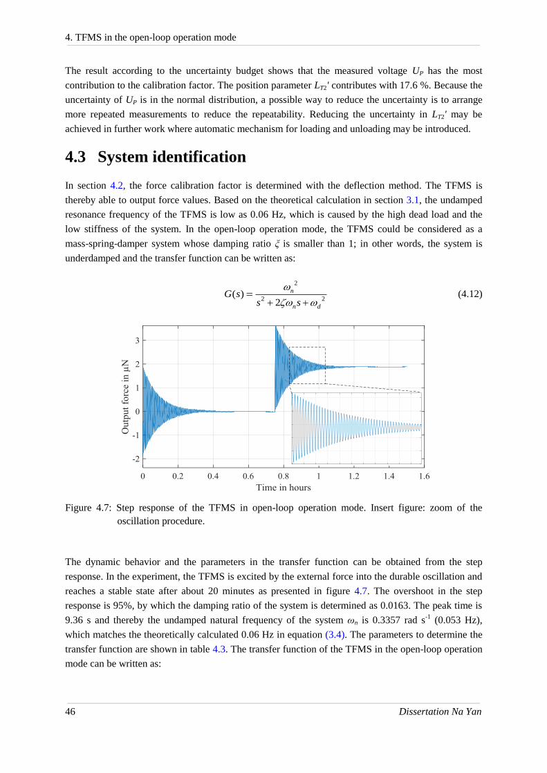
4. TFMS in the open-loop operation mode
46 Dissertation Na Yan
The result according to the uncertainty budget shows that the measured voltage UP has the most
contribution to the calibration factor. The position parameter LT2' contributes with 17.6 %. Because the
uncertainty of UP is in the normal distribution, a possible way to reduce the uncertainty is to arrange
more repeated measurements to reduce the repeatability. Reducing the uncertainty in LT2' may be
achieved in further work where automatic mechanism for loading and unloading may be introduced.
4.3 System identification
In section 4.2, the force calibration factor is determined with the deflection method. The TFMS is
thereby able to output force values. Based on the theoretical calculation in section 3.1, the undamped
resonance frequency of the TFMS is low as 0.06 Hz, which is caused by the high dead load and the
low stiffness of the system. In the open-loop operation mode, the TFMS could be considered as a
mass-spring-damper system whose damping ratio ξ is smaller than 1; in other words, the system is
underdamped and the transfer function can be written as:
2
2 2( )
2
n
n d
G ss s
(4.12)
Figure 4.7: Step response of the TFMS in open-loop operation mode. Insert figure: zoom of the
oscillation procedure.
The dynamic behavior and the parameters in the transfer function can be obtained from the step
response. In the experiment, the TFMS is excited by the external force into the durable oscillation and
reaches a stable state after about 20 minutes as presented in figure 4.7. The overshoot in the step
response is 95%, by which the damping ratio of the system is determined as 0.0163. The peak time is
9.36 s and thereby the undamped natural frequency of the system ωn is 0.3357 rad s-1
(0.053 Hz),
which matches the theoretically calculated 0.06 Hz in equation (3.4). The parameters to determine the
transfer function are shown in table 4.3. The transfer function of the TFMS in the open-loop operation
mode can be written as:

4. TFMS in the open-loop operation mode
Dissertation Na Yan 47
2
2 2 2
0.1127( )
2 0.011 0.1126
n
n d
G ss s s s
Table 4.3: Parameters determined by step response for obtaining the transfer function.
Term Value
Percent overshoot PO
max 100%ss
ss
y y
y
95%
Peak time Tp --- 9.36 s
Damping ration ζ 2
exp[ ]1
PO
0.0163
Natural frequency ωn 21pT
0.3357 rad s
-1
Damped natural frequency ωd 2
1n 0.3356 rad s-1
Settling time
(with 5% error tolerance)
τ =2
ln(0.05 1 )
d
547 s
In figure 4.8, the Bode diagram obtained using the transfer function is presented to describe the
dynamic behavior of the TFMS in its open-loop operation mode. In the upper figure, near the natural
frequency the magnitude of the signal is distorted; in a frequency range higher than the natural
frequency, the magnitude is attenuated strongly. The cutoff frequency, which describes that the
response of the external load remains in the permissible error band of the final normalized value, is
necessary to be defined. Corresponding to the settling time, the cutoff frequency within the 5% error
tolerance is 0.002 Hz. Based on this value, a PID-controller is expected to be built with which the
TFMS can operate in the closed-loop operation mode where the dynamic behavior of the TFMS is
improved.
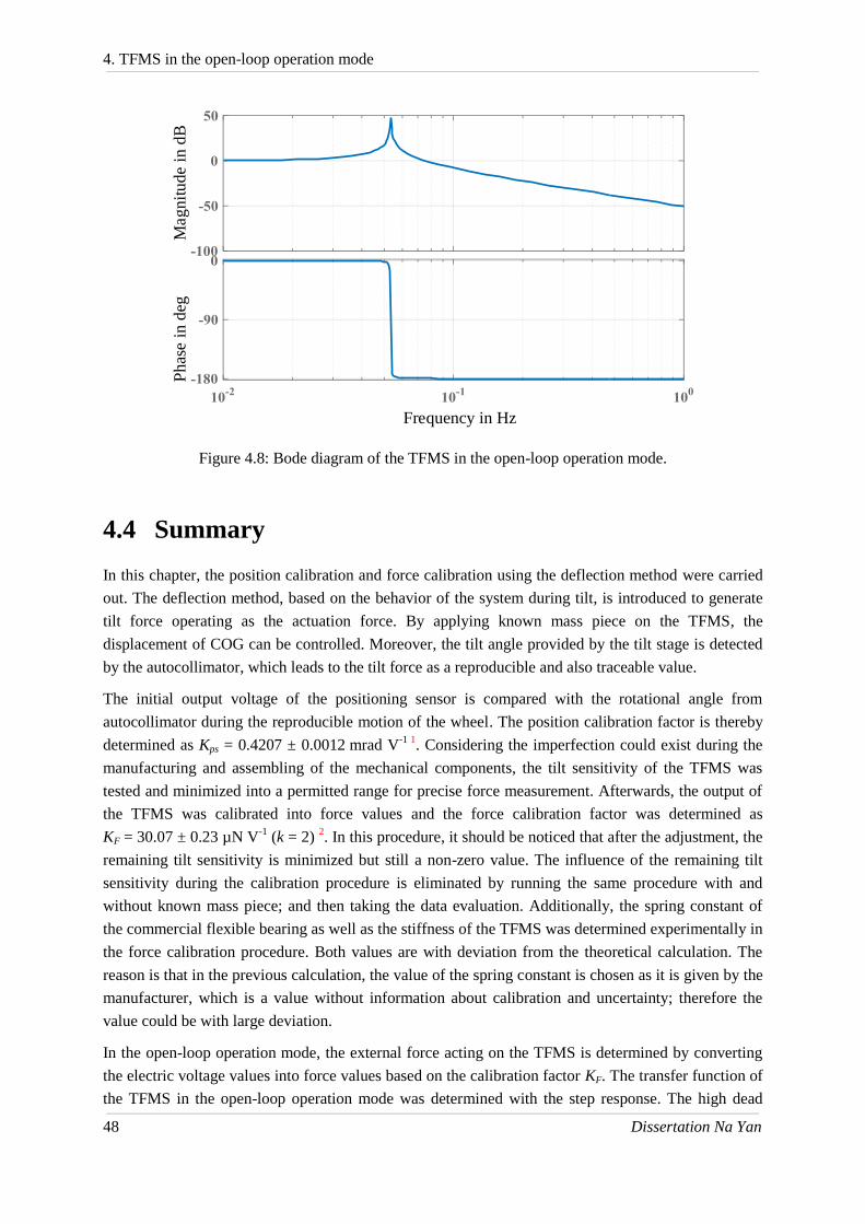
4. TFMS in the open-loop operation mode
48 Dissertation Na Yan
Figure 4.8: Bode diagram of the TFMS in the open-loop operation mode.
4.4 Summary
In this chapter, the position calibration and force calibration using the deflection method were carried
out. The deflection method, based on the behavior of the system during tilt, is introduced to generate
tilt force operating as the actuation force. By applying known mass piece on the TFMS, the
displacement of COG can be controlled. Moreover, the tilt angle provided by the tilt stage is detected
by the autocollimator, which leads to the tilt force as a reproducible and also traceable value.
The initial output voltage of the positioning sensor is compared with the rotational angle from
autocollimator during the reproducible motion of the wheel. The position calibration factor is thereby
determined as Kps = 0.4207 ± 0.0012 mrad V-1 1
. Considering the imperfection could exist during the
manufacturing and assembling of the mechanical components, the tilt sensitivity of the TFMS was
tested and minimized into a permitted range for precise force measurement. Afterwards, the output of
the TFMS was calibrated into force values and the force calibration factor was determined as
KF = 30.07 ± 0.23 µN V-1
(k = 2) 2. In this procedure, it should be noticed that after the adjustment, the
remaining tilt sensitivity is minimized but still a non-zero value. The influence of the remaining tilt
sensitivity during the calibration procedure is eliminated by running the same procedure with and
without known mass piece; and then taking the data evaluation. Additionally, the spring constant of
the commercial flexible bearing as well as the stiffness of the TFMS was determined experimentally in
the force calibration procedure. Both values are with deviation from the theoretical calculation. The
reason is that in the previous calculation, the value of the spring constant is chosen as it is given by the
manufacturer, which is a value without information about calibration and uncertainty; therefore the
value could be with large deviation.
In the open-loop operation mode, the external force acting on the TFMS is determined by converting
the electric voltage values into force values based on the calibration factor KF. The transfer function of
the TFMS in the open-loop operation mode was determined with the step response. The high dead
Magnit
ude i
n d
BP
has
e i
n d
eg
Frequency in Hz

4. TFMS in the open-loop operation mode
1,2 The value differs from that determined in the previous work [44], because the TFMS was once disassembled
for another low temperature test. The geometry could change after reassembling.
Dissertation Na Yan 49
load and low stiffness of the system lead to a low natural frequency; additionally, the damping ratio of
the TFMS is also low as 0.0163. Both effects result into the long response time of over 500 s. With the
aim to improve the dynamic behavior, the closed-loop operation mode based on the PID-controller is
set up, which will be introduced in the chapter 5.

5. TFMS in the closed-loop operation mode
50 Dissertation Na Yan
5. TFMS in the closed-loop operation mode
In chapter 4, experiments and calculations were carried out on the TFMS to determine the transfer
function in its open-loop operation mode. Aiming to improve the dynamic properties of the TFMS, the
closed-loop operation mode is set up. Figure 5.1 presents an overview of the work in this chapter.
Figure 5.1: Block diagram giving an overview of work in chapter 5. The closed-loop operation mode
is set up based on PID-controller. Commercial voice coil actuator generates
electromagnetic force (EMF) as the compensation force. The EMF is calibrated using
deflection method. The customized capacitive actuator is built to provide electrostatic
force (ESF) as an alternative way to perform compensation force. The ESF is calibrated
with three methods which will be introduced in section 5.3.
The closed-loop operation mode is set up in section 5.1, with electromagnetic force (EMF) as the
compensation force by using a commercial voice coil actuator. The force constant of the voice coil
actuator is determined using the deflection method. In section 5.2, a customized plate-shaped capacitor
Open-loop
(Chapter 4)Closed-loop
TFMS
EMF ESF
Deflection
method
Operation mode
Force actuator
Calibration Calibration
Measuring
capacitance
gradient
Comparing
with
EMF
Measuring
induced current
Commercial
voice coil
actuator
Customized
capacitive
actuator
a) b) c)

5. TFMS in the closed-loop operation mode
Dissertation Na Yan 51
is introduced to generate the electrostatic force (ESF), which is considered as a reasonable replacement
of the EMF. Afterwards, three methods for the calibration of the ESF are introduced in the section 5.3,
they are:
a) Calibration by measuring capacitance gradient;
b) Calibration by comparing with the EMF as the reference force;
c) Calibration by measuring induced current when the TFMS operates in a velocity mode.
At the end of this chapter, the dynamic and static properties of the TFMS are tested respectively in
section 5.4 and 5.5.
5.1 Setting up PID-controller using electromagnetic force
In the open-loop operation mode presented in figure 5.2, the motion of the TFMS caused by external
force is detected by the positioning sensor. The force value is calculated from the initial output voltage
UP and the calibration factor KF determined in section 4.2.
Figure 5.2: Block diagram of the TFMS in the open-loop operation mode and closed-loop operation
mode using PID-controller.
As a result of the dead load caused by the dummy weights and the low stiffness enabled by the
sensitive flexible bearing, the undamped natural frequency of the system is as low as approximately
0.06 Hz. Moreover, the damping ratio of the TFMS is also minimal at 0.0163, which leads to the
durable oscillation when the TFMS is excited by external signal as figure 4.7 presents. In the
measurement of static force with the load frequency ≤ 0.002 Hz, the open-loop operation mode is
acceptable. However, when the load frequency is higher than 0.002 Hz, the magnitude of the output
starts to be distorted, and damped strongly when the load frequency is higher than 0.06 Hz. In the LFV
application to monitor the production process, the mean velocity of the conducting flows is quasi
constant leading to the static Lorentz force. Therefore, the dynamic property of the force measurement
system is not a crucial point. However, the dynamic behavior is still expected to be improved under
the premise that force resolution is maintained. The closed-loop operation mode is set up based on the
PID-controller.
TFMSe(t)
PIDIc
Voice
coil
actuator
Fc UPUP0
Measurements
-
UP(t)
Compute
F = KF ∙ UP
open-loop
closed-loop
Capacitive
actuator
Fes
F ~ Fc

5. TFMS in the closed-loop operation mode
52 Dissertation Na Yan
As demonstrated in figure 5.2, similar to the working principle of the EMFC weighing cell, in the
closed-loop operation mode the deflection of the TFMS caused by external force is continuously
compensated by force Fc. A commercial voice coil actuator similar to the one integrated inside the
EMFC weighing cell, is utilized to generate the electromagnetic compensation force. The voice coil
actuator consists of a magnet and coil wire immersed in the magnetic field. The voice coil actuator is
assembled to the TFMS as presented in figure 5.3: the coil wire is screwed on the arm of the plane
wheel while the magnet is carefully aligned to the coil and fixed on the base plate. By supplying
electric current Ic to the coil, the electromagnetic force based on equation (1.4) is generated between
the coil and magnet, namely, the electromagnetic force acts on the TFMS. The original power cables
of the coil provided by the manufacturer are replaced by the very thin copper wires with the diameter
of 50 µm, carrying the electric current Ic in the range of microampere supplied by the universal source
HP 3245A [46]. As the coil is assembled to the rotational component of the TFMS, reducing the
diameter of the cables by using the thin wires can minimize the undesired forces caused by the
stiffness of the cables. Exchanging the position of the magnet and the coil is not desired as the
magnetic interaction could influence the motion of the TFMS when the magnet is assembled on the
plane wheel.
Figure 5.3: Commercial voice coil actuator assembled on the TFMS, providing electromagnetic
compensation force for the closed-loop operation mode.
The PID-controller is used to calculate the required compensation current Ic in order to perform the
compensation procedure. As demonstrated in figure 5.2, initially a voltage value UP0 is defined for the
null position of the plane wheel. The value UP0 can be manually given as zero indicating the
geometrical center position or any other non-zero values indicating offset from the geometrical center.
The value of UP0 can also be taken as the mean value of a period of pre-measurement in the open-loop
operation mode, which describes the natural static position of the TFMS. When the wheel deflects
from the defined null position due to external forces, the value e(t) as the difference between the real
time measured voltage UP(t) and the defined value UP0 is calculated and transferred to the PID-
controller to determine the compensation current Ic. The parameters of the PID-controller is firstly
determined with MatLab application system identification based on the step response of the TFMS in
NS
Ic Fc
d
d = 15.9mm x
y
Lc

5. TFMS in the closed-loop operation mode
Dissertation Na Yan 53
its open-loop, and adjusted then experimentally to obtain faster response and also stability. The
electric current Ic is applied to the commercial voice coil actuator to generate the electromagnetic force
as the compensation force Fc bringing the TFMS from deflection back to its null position.
Figure 5.4: Step response of the TFMS in the closed-loop operation mode based on PID-controller and
electromagnetic compensation force. (a) Output voltage of the positioning sensor UP (t)
indicating that the wheel is continuously compensated back to the null position; (b) Motion
of the plane wheel around x- and y-axis detected by the autocollimator which indicates that
the plane wheel remaining stable in the xy-plane; (c) Compensation current Ic for
generating compensation force; (d) Highlighted control procedure. The horizontal scale of
all four figures is given as: Time in seconds.
Figure 5.4 presents the experimental data describing the control procedure. The TFMS in the closed-
loop operation mode is excited by external force. Figure 5.4 (a) presents the output voltage UP(t)
indicating the position of the plane wheel. Due to the PID-controller, the plane wheel is continuously
compensated back to the null position which is defined by the voltage UP0. In this test, the UP0 is given
as 0 V as demonstrated in the insert figure. The measured UP(t) oscillates around the value UP0 in the
range of ± 10 µV, which can be considered as stable due to that the voltage value of 10 µV
corresponds to the position change of < 1 nm. The figure 5.4 (c) presents the required compensation
current Ic to compensate the deflection caused by external forces, and the highlighted control
procedure is presented in figure 5.4 (d). In this experiment, the settling time of the TFMS in closed-
loop operation is about 9.2 s with 5% error tolerance. Additionally, in the test of the closed-loop
operation mode, the autocollimator is assembled to the system in a suspended configuration, aiming to
record the undesired motion of the plane wheel around x- and y-axis. The measured data shown in
figure 5.4 (b) presents a stable signal with a standard deviation of 0.06 arcsec and 0.1 arcsec of the
(a) (b)
(c) (d)
Ou
tput
vo
ltag
e
(UP(t
)) i
n m
V
Around y
Around x
Co
mp
ensa
tio
n
Cu
rren
t I c
in
µA
An
gle
of
the
wh
eel
in µ
rad
UP0 = 0 V
0.02
0.01
0
-0.01
-0.02

5. TFMS in the closed-loop operation mode
54 Dissertation Na Yan
rotational angle around x- and y-axis, which proves that during operation the wheel remains
considerably stable in the xy-plane.
After setting up the closed-loop operation mode, the measured force values are no longer calculated
with the output voltage UP and the calibration factor KF, but described by the compensation force Fc,
which is obtained by the compensation current Ic and the force constant of the voice coil actuator Kvc.
The force constant of the actuator given by the manufacturer is Kvc = 1.1 N A-1
[45]. However, in real
cases the force constant could deviate from the given value because of alignment errors and different
immersion depths of the coil into the magnetic field. For example, in work [29], the force constant of
the same voice coil actuator was determined as 0.93 N A-1
. In [47] the force constant with different
immersion depths of a similar kind of actuator is tested with a micro stage and the EMFC weighing
cell. In that test, the measured data reveals that a change of 1 mm in the immersion depth leads to the
relative change in force constant of more than 2.5%. Therefore, after local alignment and assembling,
the force constant of the voice coil actuator used in this work is expected to be determined. This
procedure can also be achieved by using the deflection method introduced in chapter 4. The traceable
tilt force is generated on the TFMS by using tilt stage and the standard weight. In this experiment, the
PID-controller is switched on. The required compensation current Ic is continuously recorded during
the compensation of the tilt force. The force constant of the voice coil actuator Kvc in the work is
determined experimentally as:
1sin Tvc
c c
m g LK
I L
(5.1)
The result presented in table 5.1 is obtained concerning the uncertainty contribution of the following
parameters:
The mass m is 1 g standard weight piece from class E2, the maximum permissible error is
0.03 mg;
The gravitational acceleration g was once measured in the laboratory locally, the value and its
uncertainty are taken from the certificate;
The tilt angle α is measured by the autocollimator, the mean value and uncertainty are
determined by repeated measurements.
The three parameters mentioned above determine the quality of the generated tilt force.
And additionally:
The compensation current Ic is also determined as the mean value of repeated measurements;
The arm length of the voice coil actuator Lc, and LT1 indicating the position where tilt force is
applied, the permissible error of both is 0.5 mm.
The uncertainty budget presents that the uncertainty in the obtained force constant comes mostly from
the repeatability of the compensation current. The force constant of the voice coil actuator with the
local alignment is experimentally determined as Kvc = 0.869 ± 0.038 N A-1
. Thus, the compensation

5. TFMS in the closed-loop operation mode
Dissertation Na Yan 55
current Ic presented in figure 5.4 (c) can be transferred to force values and TFMS can output forces in
the closed-loop operation mode.
Table 5.1: Uncertainty budget of the force constant Kvc of the voice coil actuator.
Quantity [unit]
Value
Standard
Uncertainty
Distribution
Sensitivity
coefficient
Index
m [kg] 1·10-3
1.73·10-8
rectangular 870 0 %
g [m s-2
] 9.81015772 0.11·10-6
normal 0.089 0 %
α [rad] 6·10-3
0.351·10-6
normal 150 0 %
LT1 [mm] 180 0.289 rectangular 0.0048 0.6 %
Lc [mm] 59.5 0.289 rectangular -0.015 5.2 %
Ic [A] 2.05·10-4
4.22·10-6
normal -4200 94.2 %
Result Kvc = 0.869 ± 0.038 N A-1
(k = 2) (relative uncertainty: 4.4 %)
5.2 Setting up electrostatic force generator
By setting up the closed-loop operation mode based on PID-controller, the dynamic property of the
TFMS is improved. However, there are still some imperfections by using the electromagnetic force as
the compensation force because: (1) the stiffness of the thin copper wires as the power cables of the
voice coil actuator is small but not zero. Motion of the wires can influence the measurement of the
TFMS; (2) in the later application as part of the LFV, a magnet system is involved which is supported
by the TFMS, providing the magnetic field and carrying the force to be measured. Under this
condition, by using the voice coil actuator, electromagnetic interaction can influence the measurement;
(3) the TFMS developed in this work is expected to be reduced in dimensions to build a second
generation system. In the future, the second generation system will cooperate with high-temperature
superconducting (HTS) bulks as quasi-permanent magnets [48], replacing the current used magnet
system. In the design concept, the second generation TFMS together with the HTS bulks will be
assembled inside a cryostat and brought to magnetization in the strong magnetic field, in which case
the voice coil actuator as part of the TFMS will be also magnetized and not in the condition to provide
traceable compensation forces. Due to the three reasons mentioned above, the voice coil actuator is
thereby urged to be replaced. The development introduced in this section intends to find a reasonable
replacement of the voice coil actuator, namely, to find other kinds of force which could operate as the
compensation force for the TFMS and replace the electromagnetic force.
In several researches on small force metrology [12-18], the electrostatic force has been introduced. A
brief introduction is presented earlier in section 1.2.1. By applying actuation voltage Ua across the two
electrodes of the capacitor, electrostatic force Fes is induced between the two electrodes as equation

5. TFMS in the closed-loop operation mode
56 Dissertation Na Yan
(5.2) presents. Based on the mechanical construction of the TFMS, a customized capacitive force
actuator is set up and is introduced in this section.
21
2es a
dCF U
dx (5.2)
All the mechanical components of the TFMS are made of metal: dummy weights made of copper, the
commercial flexible bearing from stainless steel, the material of all the other mechanical components
manufactured in the workshop from aluminum AW 7075 alloy. Moreover, all screws for fixing are
from brass. This makes the TFMS as one conductor, which can be further considered as one electrode
of a capacitor. A rectangular printed circuit board (PCB) presented in figure 5.5(b) is fixed near and
facing the dummy weight and connected to the anode of the signal generator as demonstrated in figure
5.5. The base plate of the TFMS is grounded and connected to the cathode of the signal generator.
Since the TFMS is one conductor, the electric potential at each part of the TFMS is same and equals to
the cathode. The PCB as one electrode, the section of the dummy weight facing against the PCB as the
second electrode and together with the air in between is in the structure of a plate-shaped capacitor.
Electrostatic force Fes is induced by applying the actuation voltage Ua across the two electrodes. Thus,
the customized capacitive force actuator is built without assembling additional components on the
rotational part of the TFMS. Electrostatic force is controllable by adjusting the actuation voltage Ua.
Figure 5.5: Setting up a capacitive actuator to generate electrostatic force on the TFMS. (a) Overview.
(b) The customized rectangular PCB plate. (c) The PCB is located facing the dummy
weight with a small distance, in between is air. By supplying actuation voltage across the
PCB and TFMS, the electrostatic force is thereby generated.
Signal
Generator
- + - +
Fes
Fc
Ic
Ua
Ch-ACh-B
.
x
yz
Les
Lc
(c)
(b)
(a)

5. TFMS in the closed-loop operation mode
Dissertation Na Yan 57
5.3 Calibration of electrostatic force
Equation (5.2) indicates that the induced electrostatic force Fes is proportional to the second power of
the applied actuation voltage Ua across the two electrodes, and the calibration factor Kes depends on
the capacitance gradient described by equation (5.3):
2
es es aF K U with 1
2es
dCK
dx (5.3)
To actuate traceable electrostatic force, the calibration factor Kes is necessary to be determined. In this
section, three methods are introduced to implement the calibration of the electrostatic force. The block
scheme describing the following three methods is shown in figure 5.6, they are:
(a) Determining the force calibration factor Kes by measuring capacitance values with different
distances between the two electrodes (determining capacitance gradient);
(b) Determining the force calibration factor Kes by comparing the electrostatic force with the
reference force -- electromagnetic force;
(c) Determining the force calibration factor Kes by measuring induced current during the TFMS
operating in a velocity mode.
Figure 5.6: Determining the calibration factor with three methods: (a) Measuring capacitance values C
with different distances dx for obtaining capacitance gradient; (b) Recording the
compensation force with different actuation voltage Ua across the two electrodes, in order
to compare the electrostatic forces Fes with electromagnetic forces Fem; (c) The PID-
controller is shut down and the TFMS is set into a velocity mode, the calibration factor is
determined by measuring the induced current i(t).
TFMS
PID on
PID off
dx (~ UP0)
HiokiC
Voice coil
actuator
Fem
Voice coil
actuator
d0 + ds
Voltage
source
Ua
(stepwise)
Voltage
source
Ua
(constant)
a)
b)
c)
Kes = Ua
2· Les
Fem ·Lc
Kes = 2·Ua· ds
i(t).
ds
.
Kes = 21
dx
dC
Ia
·

5. TFMS in the closed-loop operation mode
58 Dissertation Na Yan
5.3.1 Three methods to calibrate the electrostatic force
Method (a): By measuring the capacitance values with different distance values:
This method is based on the equation (5.2) and (5.3) as general equations to generate the electrostatic
force, where the force calibration factor Kes is described by the capacitance gradient dC/dx as
presented in equation (5.4). The capacitance of the capacitor is dependent on the distance between the
two electrodes, namely the distance between the PCB and the dummy weight in x-direction. A is the
effective cross section of the customized capacitor. Between the two electrodes is air under the room
temperature, relative permittivity εr is 1.00053. d0 is the initial distance between the two electrodes and
ds indicates the change of the distance in the x-direction.
0
2
0
1 1
2 2 ( )
res
s
AdCK
dx d d
(5.4)
In several work [16,18], for calibration of the electrostatic force, the distance between the two
electrodes is adjusted by driving one of the electrodes to different positions using a piezo stage or an
auxiliary capacitor. In comparison, as the motion of the TFMS can be controlled in its closed-loop
operation mode, the dummy weight as one electrode can be set to different positions by giving
different defined values UP0 in the PID-controller. Thereby, the distance dx between the dummy weight
and the PCB as the summation of d0 and ds can be adjusted and controlled. The value of the distance
can be calculated with equation (5.5).
0 0( )x s P P ps esd d d U U ' K L
0 (0 )P ps es P ps esd U ' K L U ' K L (5.5)
UP0 is the value given to the PID-controller and defines the position to be maintained in the
compensation procedure. By setting different values of UP0, the value dx as the distance between the
two electrodes of the capacitor changes along with it. d0 indicates the distance between the two
electrodes when the value UP0 of zero is given. UP' is the output voltage of the positioning sensor when
the wheel is at the position where the dummy weight touches the PCB (namely, dx = 0). The factor Kps
obtained in section 4.1 is the calibration factor to convert the voltage values into rotational angles and
Les illustrated in figure 5.5 is the distance of the customized capacitor away from the rotational axis of
the TFMS. With the known values of UP', Kps and Les, the initial distance d0 is determined as
approximately 124 µm.
According to the rough calculation with the parameters of the customized capacitor, the capacitance
value is in the range of dozens picofarad and can be measured by the device Hioki impedance analyzer
IM-3570 [49]. In the experiment, stepwise voltage UP0 is given in the PID-controller in order to lead to
different distance values dx. The capacitance value C of the customized capacitor is measured by the
impedance analyzer with each distance value as the block diagram (a) in figure 5.6 presents. In this

5. TFMS in the closed-loop operation mode
Dissertation Na Yan 59
way the capacitance gradient is determined, which can be used to describe the calibration factor of the
electrostatic force.
Figure 5.7: Top: Measured capacitance values of the customized capacitor by setting different
distances between the two electrodes. Bottom: Determined calibration factor along with
different distance values.
Top of figure 5.7 presents the measured capacitance values by setting different distances between the
two electrodes. The capacitance value is inversely proportional to the distance dx. Due to a same
change in the separation, the closer the two electrodes are, the more rapidly the capacitance increases.
The calibration factor Kes is demonstrated in the bottom figure, the values calculated theoretically with
the parameters according to equation (5.4) as well as the experimental data are presented and show an
agreement with each other. The calibration factor depends on the distance between the two electrodes,
when UP0 = 0 V, in other words, with the separation d0, the calibration factor is:
Kes = 0.0561 ± 0.0006 µN V-2
(k = 2)
Figure 5.7 reveals that the calibration factor can be further increased by reducing the distance between
the PCB and the dummy weight. From 120 µm to 40 µm, the calibration factor is increased by 6 times.
Moreover, indicated by equation (5.4), increasing the effective section area A of the capacitor or the
relative permittivity is also a way to increase the calibration factor.
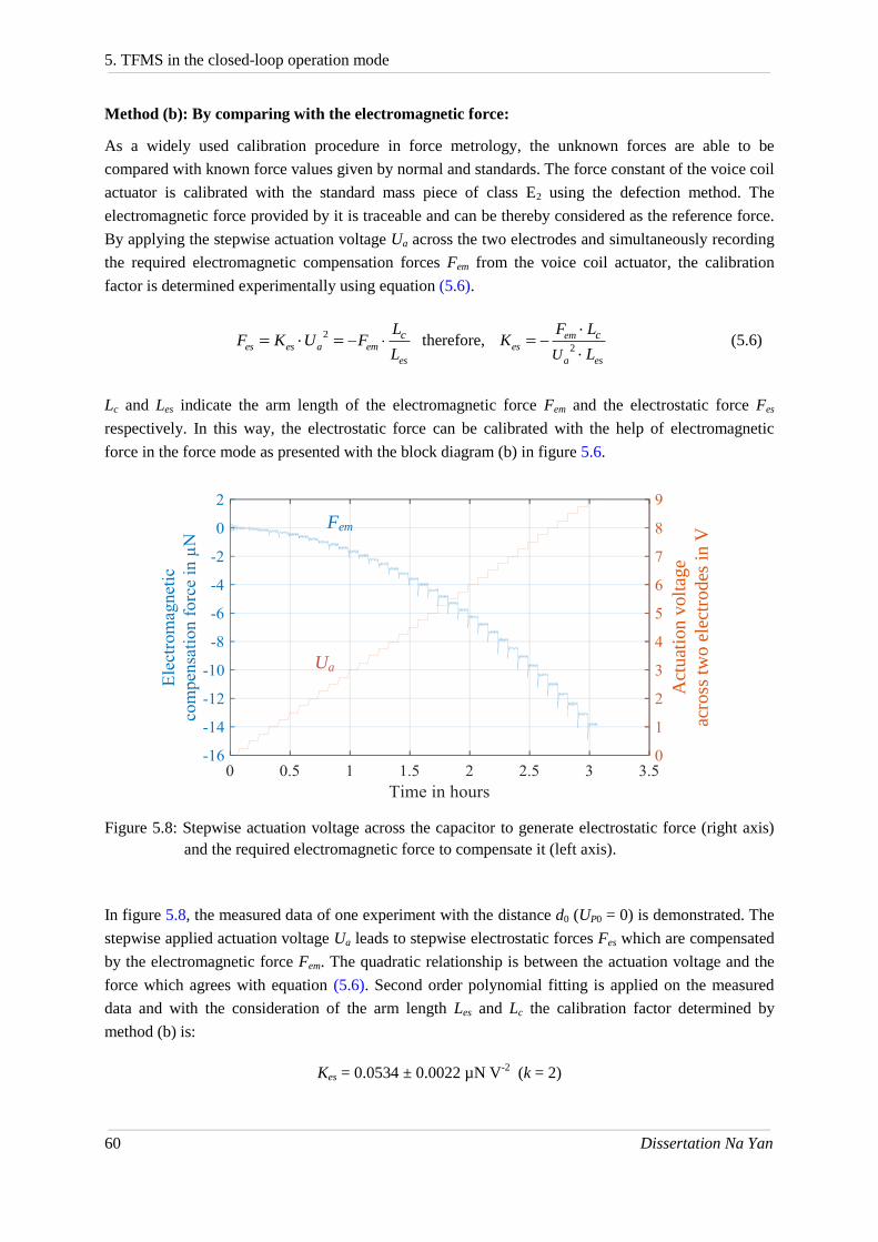
5. TFMS in the closed-loop operation mode
60 Dissertation Na Yan
Method (b): By comparing with the electromagnetic force:
As a widely used calibration procedure in force metrology, the unknown forces are able to be
compared with known force values given by normal and standards. The force constant of the voice coil
actuator is calibrated with the standard mass piece of class E2 using the defection method. The
electromagnetic force provided by it is traceable and can be thereby considered as the reference force.
By applying the stepwise actuation voltage Ua across the two electrodes and simultaneously recording
the required electromagnetic compensation forces Fem from the voice coil actuator, the calibration
factor is determined experimentally using equation (5.6).
2
es es a em
es
cLF K U F
L therefore,
2
emes
a es
c
U
F LK
L
(5.6)
Lc and Les indicate the arm length of the electromagnetic force Fem and the electrostatic force Fes
respectively. In this way, the electrostatic force can be calibrated with the help of electromagnetic
force in the force mode as presented with the block diagram (b) in figure 5.6.
Figure 5.8: Stepwise actuation voltage across the capacitor to generate electrostatic force (right axis)
and the required electromagnetic force to compensate it (left axis).
In figure 5.8, the measured data of one experiment with the distance d0 (UP0 = 0) is demonstrated. The
stepwise applied actuation voltage Ua leads to stepwise electrostatic forces Fes which are compensated
by the electromagnetic force Fem. The quadratic relationship is between the actuation voltage and the
force which agrees with equation (5.6). Second order polynomial fitting is applied on the measured
data and with the consideration of the arm length Les and Lc the calibration factor determined by
method (b) is:
Kes = 0.0534 ± 0.0022 µN V-2
(k = 2)
Fem
UaA
ctu
atio
n v
olt
age
acro
ss t
wo
ele
ctro
des
in
V

5. TFMS in the closed-loop operation mode
Dissertation Na Yan 61
The obtained calibration factor matches the one determined by method (a) well. Moreover, similar to
that in method (a), the calibration procedure is implemented with different distances between the two
electrodes by setting the different value of UP0, which is presented later at the end of the section.
Method (c): By measuring induced current in a velocity mode:
In the watt balance experiment the force factor (B·L) can be dynamically determined by operating the
balance in a velocity mode and recording the induced voltage on the coil [50]. Similarly, the
customized capacitor can be arranged in the velocity mode when the wheel is driven by the voice coil
actuator moving relatively to the PCB plate (PID-controller is shut down). Due to the relative motion,
the current i(t) is induced and can be measured through a resistor. Constant actuation voltage Ua is
applied across both electrodes of the capacitor, the induced current as the time-derivative of the charge
Q is described as equation (5.7):
0
2
0
( )( )
( )
a a a r sa a
s
d C U dU U A ddQ dC dCi t C U U
dt dt dt dt dt d d
(5.7)
Where A indicates the section area of the capacitor, d0 is the initial distance of the two plates in static
status and ds describes the motion of the wheel in dynamic case; ds presents the velocity of the motion.
Based on equation (5.4) and (5.7) the force calibration factor Kes can be described as equation (5.8):
0
2
0
( )
( )2
1
2es
r
sa s
A i tK
d dU d
(5.8)
The experimental procedure is demonstrated in figure 5.6 block diagram (c). Current source supplies
sinusoidal actuation current Ia to the voice coil, leading the plane wheel of the TFMS into the
sinusoidal motion. This motion is detected by the positioning sensor, by which the velocity of the
dummy weight as one electrode of the capacitor is determined as the time-derivative of the position.
Across the capacitor the constant voltage Ua of 5 V is supplied. Due to the slow response of the TFMS
in its open-loop mode, high velocity motion is not achievable because the amplitude of the motion is
strongly damped when the frequency is higher than the resonance frequency. The actuation current is
set with the amplitude of 50 µA and frequency of 0.06 Hz. The induced current is in the range of pico-
ampere due to the low velocity and measured by measuring the voltage drop Um upon a resistor Rr. In
order to amplify the voltage, a resistor of 4 MΩ is connected to the capacitor. The multimeter with an
inner resistor of 1 MΩ is connected to the resistor Rr in a parallel circuit to measure the voltage drop
Um. The effective resistor Rr' is thereby reduced from 4 MΩ to 0.8 MΩ.
Figure 5.9 demonstrates the measured and analytical results. Due to the sinusoidal actuation current,
the TFMS is driven into the sinusoidal motion with the displacement and the velocity shown in the
upper figure. With equation (5.7), the induced current i(t) is determined theoretically with the value of
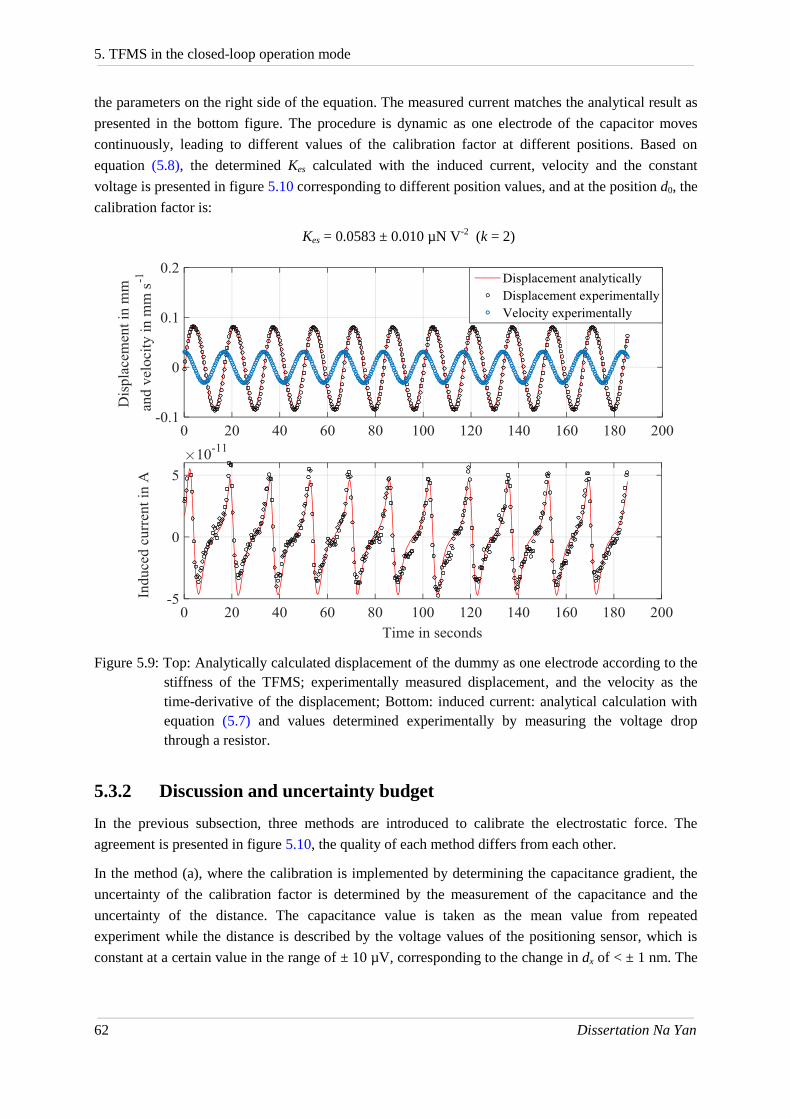
5. TFMS in the closed-loop operation mode
62 Dissertation Na Yan
the parameters on the right side of the equation. The measured current matches the analytical result as
presented in the bottom figure. The procedure is dynamic as one electrode of the capacitor moves
continuously, leading to different values of the calibration factor at different positions. Based on
equation (5.8), the determined Kes calculated with the induced current, velocity and the constant
voltage is presented in figure 5.10 corresponding to different position values, and at the position d0, the
calibration factor is:
Kes = 0.0583 ± 0.010 µN V-2
(k = 2)
Figure 5.9: Top: Analytically calculated displacement of the dummy as one electrode according to the
stiffness of the TFMS; experimentally measured displacement, and the velocity as the
time-derivative of the displacement; Bottom: induced current: analytical calculation with
equation (5.7) and values determined experimentally by measuring the voltage drop
through a resistor.
5.3.2 Discussion and uncertainty budget
In the previous subsection, three methods are introduced to calibrate the electrostatic force. The
agreement is presented in figure 5.10, the quality of each method differs from each other.
In the method (a), where the calibration is implemented by determining the capacitance gradient, the
uncertainty of the calibration factor is determined by the measurement of the capacitance and the
uncertainty of the distance. The capacitance value is taken as the mean value from repeated
experiment while the distance is described by the voltage values of the positioning sensor, which is
constant at a certain value in the range of ± 10 µV, corresponding to the change in dx of < ± 1 nm. The
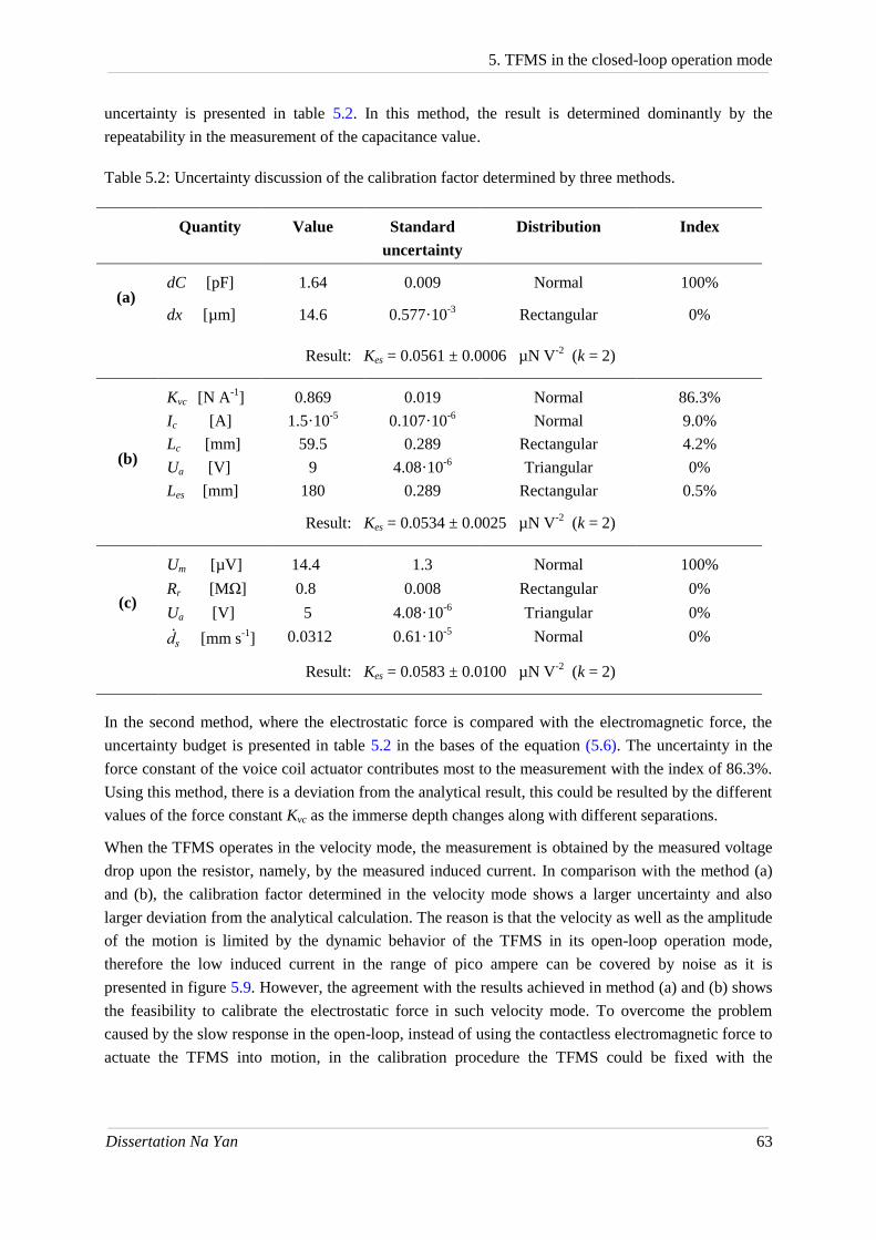
5. TFMS in the closed-loop operation mode
Dissertation Na Yan 63
uncertainty is presented in table 5.2. In this method, the result is determined dominantly by the
repeatability in the measurement of the capacitance value.
Table 5.2: Uncertainty discussion of the calibration factor determined by three methods.
Quantity Value Standard
uncertainty
Distribution Index
(a) dC [pF] 1.64 0.009 Normal 100%
dx [µm] 14.6 0.577·10-3
Rectangular
0%
Result: Kes = 0.0561 ± 0.0006 µN V-2
(k = 2)
(b)
Kvc [N A-1
] 0.869 0.019 Normal 86.3%
Ic [A] 1.5·10-5
0.107·10-6
Normal 9.0%
Lc [mm] 59.5 0.289 Rectangular 4.2%
Ua [V] 9 4.08·10-6
Triangular 0%
Les [mm] 180 0.289 Rectangular 0.5%
Result: Kes = 0.0534 ± 0.0025 µN V-2
(k = 2)
(c)
Um [µV] 14.4 1.3 Normal 100%
Rr [MΩ] 0.8 0.008 Rectangular 0%
Ua [V] 5 4.08·10-6
Triangular 0%
ds [mm s-1
] 0.0312 0.61·10-5
Normal 0%
Result: Kes = 0.0583 ± 0.0100 µN V-2
(k = 2)
In the second method, where the electrostatic force is compared with the electromagnetic force, the
uncertainty budget is presented in table 5.2 in the bases of the equation (5.6). The uncertainty in the
force constant of the voice coil actuator contributes most to the measurement with the index of 86.3%.
Using this method, there is a deviation from the analytical result, this could be resulted by the different
values of the force constant Kvc as the immerse depth changes along with different separations.
When the TFMS operates in the velocity mode, the measurement is obtained by the measured voltage
drop upon the resistor, namely, by the measured induced current. In comparison with the method (a)
and (b), the calibration factor determined in the velocity mode shows a larger uncertainty and also
larger deviation from the analytical calculation. The reason is that the velocity as well as the amplitude
of the motion is limited by the dynamic behavior of the TFMS in its open-loop operation mode,
therefore the low induced current in the range of pico ampere can be covered by noise as it is
presented in figure 5.9. However, the agreement with the results achieved in method (a) and (b) shows
the feasibility to calibrate the electrostatic force in such velocity mode. To overcome the problem
caused by the slow response in the open-loop, instead of using the contactless electromagnetic force to
actuate the TFMS into motion, in the calibration procedure the TFMS could be fixed with the
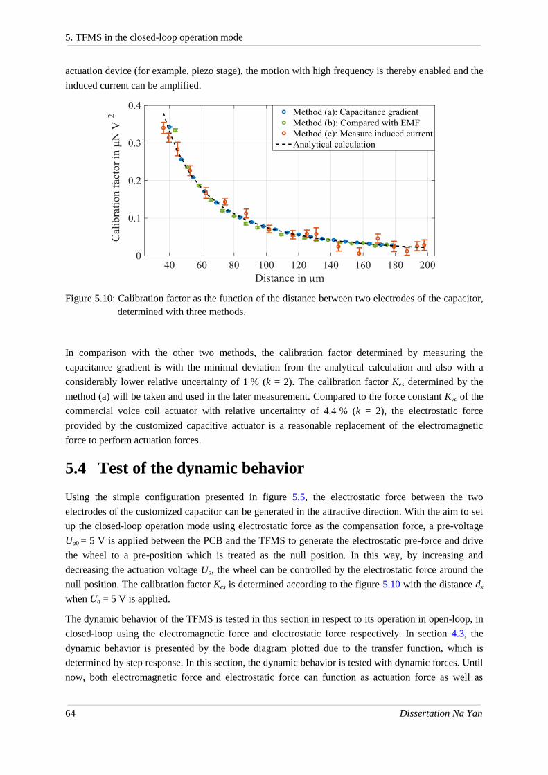
5. TFMS in the closed-loop operation mode
64 Dissertation Na Yan
actuation device (for example, piezo stage), the motion with high frequency is thereby enabled and the
induced current can be amplified.
Figure 5.10: Calibration factor as the function of the distance between two electrodes of the capacitor,
determined with three methods.
In comparison with the other two methods, the calibration factor determined by measuring the
capacitance gradient is with the minimal deviation from the analytical calculation and also with a
considerably lower relative uncertainty of 1 % (k = 2). The calibration factor Kes determined by the
method (a) will be taken and used in the later measurement. Compared to the force constant Kvc of the
commercial voice coil actuator with relative uncertainty of 4.4 % (k = 2), the electrostatic force
provided by the customized capacitive actuator is a reasonable replacement of the electromagnetic
force to perform actuation forces.
5.4 Test of the dynamic behavior
Using the simple configuration presented in figure 5.5, the electrostatic force between the two
electrodes of the customized capacitor can be generated in the attractive direction. With the aim to set
up the closed-loop operation mode using electrostatic force as the compensation force, a pre-voltage
Ua0 = 5 V is applied between the PCB and the TFMS to generate the electrostatic pre-force and drive
the wheel to a pre-position which is treated as the null position. In this way, by increasing and
decreasing the actuation voltage Ua, the wheel can be controlled by the electrostatic force around the
null position. The calibration factor Kes is determined according to the figure 5.10 with the distance dx
when Ua = 5 V is applied.
The dynamic behavior of the TFMS is tested in this section in respect to its operation in open-loop, in
closed-loop using the electromagnetic force and electrostatic force respectively. In section 4.3, the
dynamic behavior is presented by the bode diagram plotted due to the transfer function, which is
determined by step response. In this section, the dynamic behavior is tested with dynamic forces. Until
now, both electromagnetic force and electrostatic force can function as actuation force as well as

5. TFMS in the closed-loop operation mode
Dissertation Na Yan 65
compensation force. To test the dynamic behavior of the TFMS with electromagnetic force as the
compensation force, the electrostatic forces with different loading frequencies generated by the
customized capacitive actuator act as external actuation forces. In contrast, the electromagnetic forces
are applied with different loading frequencies to the TFMS while being compensated by the
electrostatic forces. In the test of operation in the open-loop, both forces can be used as external
applied force, whereas the electromagnetic force is chosen. Based on the different dynamic behavior
of the TFMS in open-loop and closed-loop, the range of the load frequency is set differently in each
case. In the open-loop, the loading frequency from 0.001 Hz to 5 Hz are tested while in the closed-
loop loading frequency up to 10 Hz is tested.
The solid lines in figure 5.11 indicate the analytically determined frequency response in each case. For
open-loop, it is plotted by the transfer function G(s) described in equation (4.12). In both cases of
closed-loop, the transfer function Φ(s) is calculated from G(s) in open-loop and the H(s) of the PID-
controller, revealed by equation (5.9) and (5.10) [51]. KP, Kd and Ki are the parameters of the PID-
controller which were experimentally determined for both cases.
( ) ip d
KH s K K s
s (5.9)
( ) ( )
( )1 ( ) ( )
G s H sΦ s
G s H s
(5.10)
Figure 5.11: Frequency response of the TFMS in open-loop and closed-loop. Solid line: analytical
calculation with transfer function; markers: experimentally determined by forces with
different load frequencies.
Phas
e i
n d
egre
eM
agnit
ude i
n d
B
Frequency in Hz

5. TFMS in the closed-loop operation mode
66 Dissertation Na Yan
The measured data presented in figure 5.11 shows agreement with the analytical calculation. After
setting up the closed-loop operation mode, the cutoff frequency is improved to approximately 0.1 Hz,
which is sufficient for the measurement in LFV application. Moreover, by using the customized
capacitive actuator to generate electrostatic compensation force, the dynamic behavior of the system is
similar to that using the commercial voice coil actuator to generate electromagnetic force.
5.5 Test of force resolution
In the current stage, the closed-loop operation mode is built and the dynamic behavior of the TFMS is
thereby improved. Additionally, the commercial voice coil actuator and customized capacitive actuator
are assembled to the TFMS, providing both possibilities to generate electromagnetic force and
electrostatic force. With such an option, smaller magnitude forces are applied and measured by the
TFMS to test the force resolution in the closed-loop operation mode. The general measurement
schematic is illustrated in figure 5.2. In this set of measurements, different values of actuation voltage
Ua are supplied to the customized capacitor. The electrostatic forces as external actuation forces are
applied on the TFMS; and the electromagnetic force is involved as the compensation force which
compensates the external electrostatic force to maintain the plane wheel at its defined null position.
For the measurement of weak forces in micro and nanonewton range, the consideration of the
influences such as the thermal and seismic drift and noises from the environment should be assumed
carefully. In several researches, differential force measurement setups were developed, with one
system measuring target signal which is distorted by noises, and an additional identical reference
system measuring such noises [26, 30]. However, without considering changes in mechanical structure
or other additions in our work, an alternative approach can be applied in the data evaluation.
The ABA (or ABBA) measurement sequence is a commonly known method used in the mass and
force metrology. The measurement is carried out in the process of measuring weight A, then weight B,
then again weight A (or unloaded (A) - loaded (B) - unloaded (A) ). Each measurement of weight A or
B lasts an equal time period. The linear drift can be then eliminated by fitting with the measured
values in the ABA procedure (details in [52]). In this case, the related data evaluation has a positive
effect to cancel out the linear drift. However, in many situations, the drift is non-linear and by running
the ABA (or ABBA) sequence measurements, the errors can still remain in the measured signal. In
case of the apparatus presented in our work, another alternative known as the newton's polynomial
interpolation (NPI) is used for estimation of the non-linear drift [53, 54].
Equation (5.11) describes the calculation method of the NPI: with a set of given data points (x0, y0), (x1,
y1),…, (xj, yj),…, (xk, yk), the non-linear polynomial fitting can be estimated in order to determine the
ungiven values N(x) on the fitting. In the force measurement, the xj indicate the time points during the
measurement procedure, while yj are the drift values. By using equation (5.11), each ungiven points on
the non-linear drift y = N(x) can be estimated.
0 0 1 0 0 0 1( ) ( , )( ) ( ,..., )( )...( )k kN x y f y y x x f y y x x x x (5.11)

5. TFMS in the closed-loop operation mode
Dissertation Na Yan 67
During the measurement period without external load/forces, the output signal of the TFMS Fout1
indicates the drift/noise FD1, which can be considered as the given values on the non-linear
polynomial fitting, as equation (5.12) shows:
1 1out DF F (5.12)
During the loading period with external force Fes acting on the TFMS, the output signal of the
TFMS Fout2 is a summation of the drift signal FD2 and the target force signal Fes as equation (5.13)
describes:
2 2out D esF F F (5.13)
At these time points, the drift values FD2 can be considered as ungiven values on the polynomial
fitting curve, but are possible to be determined by NPI with the measured data FD1 in step 1 as
known data.
Thus, the subtraction between the measured signal Fout2 and the determined drift signal FD2 is the
target force value. In this way, without using the differential force measurement system, the non-
linear drift can also be estimated and corrected by using such data evaluation.
Figure 5.12: Estimation of the drift using the NPI. Blue solid: measured signal from TFMS
(summation of external force and drift); red dashed: estimated drift using the NPI.
The more given data points used in the NPI, the more accurate unknown drift values can be estimated.
As it is presented in figure 5.12, in approximately 1 hour time period, electrostatic force is applied on
the TFMS four times with different magnitudes. Each loading period lasts for 2 minutes. Before and
after each loading, there is a period of 10 minutes with no external force, in other words, during the
time period before and after loading, the drift values are continuously recorded. The mean value of the
output signal in each time interval of 2 minutes is calculated. Using the NPI described in equation
(5.11), the drift values when forces are applied can be estimated as figure 5.12 shows. As mentioned
-2.42 µN
Fout2
FD2
Fout1 = FD1
Ev
alu
ated
fo
rce
in µ
N

5. TFMS in the closed-loop operation mode
68 Dissertation Na Yan
above, the subtraction of the measured output signal Fout2 and the estimated drift values FD2 indicate
the external electrostatic force. As the insert figure shows, without such data evaluation, the force is
distorted by the drift value of 2.42 µN, approximately 30% of the measured signal, which proves that
the necessity of using NPI.
By applying the NPI in the data evaluation, the minimally resolved force is tested on the TFMS. A set
of actuation voltage values Ua = [0.5 0.2 0.1 0.05 0.04 0.03 0.02 0.01] V are applied across the two
electrodes of the capacitor. The electrostatic forces with the related magnitudes can be generated on
the TFMS and measured by electromagnetic compensation force. The magnitude of the electrostatic
forces can be calculated with the calibration factor Kes determined with the corresponded distance. The
applied forces and the measured force values are compared with each other, measurement results are
presented in figure 5.13 and table 5.3.
Table 5.3: Comparison of the applied force values and measured force values.
Ua [V]
Applied force
[nN]
Measured force [nN]
Difference [nN] Value Uncertainty
(k = 2)
0.5 77.1 77.5 0.6 0.4
0.2 26.3 26.2 0.9 -0.1
0.1 12.2 12.0 0.4 -0.2
0.05 5.9 6.0 0.5 0.1
0.04 4.7 4.7 0.5 0
0.03 3.5 3.7 0.5 0.2
0.02 2.3 2.5 0.6 0.2
0.01 1.2 1.6 0.6 0.4
The differences between the applied force values and the experimentally measured force values are
within the range of ± 1 nN, which presents agreement with each other. The uncertainties of the
experimentally measured forces are determined by measured data from repeated measurements (k = 2).
Further tests with even lower applied electrostatic forces are carried out. However, the forces weaker
than 1.6 nN are difficult to be distinguished. In comparison with the theoretically calculated force
resolution of 0.55 nN (obtained with experimentally determined spring constant in section 4.2.2
instead of the value given by the manufacturer), the forces obtained experimentally are limited by the
influences originating from the surroundings that are typical in real laboratory conditions. After setting
up the closed-loop operation mode, the resolution of the TFMS is 2 nN by using the NPI in data
evaluation. The expanded uncertainties (k = 2) of the tested forces are also within ± 1 nN, which is
acceptable since it does not exceed the force resolution. With a maximum applied voltage Ua = 8 V in
this work, an electrostatic force of approximately of 6 µN is applied to the TFMS; this means the

5. TFMS in the closed-loop operation mode
Dissertation Na Yan 69
measurement range of the system can be described as ± 3 µN. As introduced in section 5.3, the
measuring range can be further extended by increasing calibration factor Kes, which can be achieved
by reducing the distance between the two electrodes, increasing the permittivity, or changing other
geometrical parameters of the customized capacitor.
Figure 5.13: Comparison of the applied electrostatic forces and the measured force. Green dash line:
Applied electrostatic force (values are calculated using the calibration factor Kes); blue
circle markers: measured electrostatic force using the TFMS and the newton's
polynomial interpolation in the data evaluation; red triangular markers: difference
between the applied forces and the measured forces.
5.6 Summary
In this chapter, the closed-loop operation mode was set up based on the PID-controller. In the closed-
loop operation mode, the plane wheel of the TFMS is continuously maintained at the custom-defined
null position by the compensation force. Initially, the compensation force was the electromagnetic
force provided by a commercial voice coil actuator. For the local alignment, the force constant of the
voice coil actuator is determined using the deflection method as Kvc = 0.869 N A-1
with the relative
uncertainty of 4.4 % (k = 2), which differs from the value given by the manufacturer because of the
immersion depth and errors in alignment. Then, a customized capacitive actuator was introduced to
generate electrostatic force as an alternative to provide compensation/actuation force to the TFMS. By
assembling a PCB plate connected to the anode of the voltage source, and taking the whole TFMS as
one conductor connected to the cathode of the voltage source, a customized capacitive force actuator

5. TFMS in the closed-loop operation mode
70 Dissertation Na Yan
was built as described in section 5.2. The value of the generated electrostatic force is obtained by the
actuation voltage applied across the two electrodes and the electrostatic force calibration factor Kes. In
section 5.3, three methods were presented to determine the calibration factor, they are: (a) by
measuring capacitance with different distances to obtain capacitance gradient; (b) by comparing the
electrostatic force with the electromagnetic force as the reference force; (c) by measuring the induced
current when the capacitor is set into a velocity mode. The calibration factors determined using the
three methods show agreement with each other. In comparison with method (b) and (c), by measuring
the capacitance gradient, the determined calibration factor matches the analytical result with the
minimal deviation and a considerably low uncertainty of 1 % (k = 2). Moreover, the relationship
between the calibration factor and the distance between the two electrodes of the capacitor was also
presented. The calibration factor can be further increased by modifying the geometrical parameters. In
section 5.4 the dynamic behavior of the TFMS in its open-loop operation mode, closed-loop operation
mode with electromagnetic force as well as electrostatic force as the compensation force were tested
respectively. Sinusoidal actuation signals with different load frequencies as the input were applied to
the TFMS. The response in each case was recorded and the bode diagram presented that by setting up
the closed-loop operation mode, the cutoff frequency of the system has been improved to 0.1 Hz with
the settling time of approximately 9.2 s. Additionally, the customized capacitive actuator functions as
well as the commercial voice coil actuator in the compensating procedure. It is revealed that the
electrostatic force is a reasonable replacement of the electromagnetic force with the following
improvements:
(1) More suitable for the LFV application where magnet system is involved;
(2) No power wires connected to the rotational part of the TFMS;
(3) Force constant Kes with lower relative uncertainty.
(4) Force constant Kes can be adjusted by changing the geometry of the capacitor.
Finally in this chapter, the minimally resolved force with TFMS was tested. The newton's polynomial
interpolation was used in the data evaluation to estimate the undesired drifts and noises. In this way,
the influence caused by surroundings can be compensated without assembling second additional
reference system. Considering theoretically calculated force resolution of 0.55 nN is limited by the
influences from the surroundings that are typical in real laboratory conditions, the achieved force
resolution of 2 nN is acceptable and the aim to improve the force resolution by one order of magnitude
as introduced in the chapter 1 is reached.
Another improvement considered to be made in the future is setting up the differential electrostatic
force actuator with two identical PCB plates presented in figure 5.14. With such configuration, two
capacitors C1 and C2 enable the electrostatic force perform in both directions. The pre-voltage is
thereby no more necessary and the measurement range can be extended.
The two PCBs are with identical geometry and assembled symmetrically at both sides of the copper
dummy, which indicates that the capacitance gradient of the both capacitors are equal in magnitude
and opposite in direction at the equilibrium position (ds = 0).
1 2dC dC
dx dx (5.14)
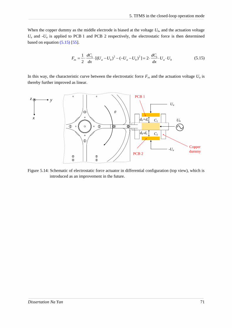
5. TFMS in the closed-loop operation mode
Dissertation Na Yan 71
When the copper dummy as the middle electrode is biased at the voltage Ub, and the actuation voltage
Ua and -Ua is applied to PCB 1 and PCB 2 respectively, the electrostatic force is then determined
based on equation (5.15) [55].
2 21 11
[( ) ( ) ] 22
es a b a b a b
dC dCF U U U U U U
dx dx (5.15)
In this way, the characteristic curve between the electrostatic force Fes and the actuation voltage Ua is
thereby further improved as linear.
Figure 5.14: Schematic of electrostatic force actuator in differential configuration (top view), which is
introduced as an improvement in the future.
.
x
yz
C1 Ub
C2
Ua
-Ua
d0+ds
d0-ds
θ
PCB 1
PCB 2
Copper
dummy

6. Lorentz force measurement
72 Dissertation Na Yan
6. Lorentz force measurement
In this Chapter, the measurements are implemented using the TFMS to measure Lorentz forces. The
TFMS operates in the closed-loop operation mode with the electrostatic force compensating external
forces. One of the two non-magnetic dummies is replaced by the magnet system providing the
magnetic field. The experimental facility is built for implementing semi-dry calibration in section 6.1.
In section 6.2, the experiments are presented, salt water as a mixture of tap water and salt (sodium
chloride) is chosen as the electrolyte. Using the semi-dry calibration, the measuring sensitivity of the
flowmeter based on the TFMS is obtained for different conductivity values.
6.1 Experimental facility
As introduced in section 1.1, the reaction force of the Lorentz force FL' acting upon the magnet system
is proportional to the flow velocity v and the electrical conductivity σ. By measuring the horizontally
directed force FL', the TFMS carrying the magnet system can measure the velocity as a flowmeter or
measure the conductivity as a conductivity meter after it is calibrated with known values. Intending to
test the performance of the TFMS for measuring FL', practical measurements with magnet system
together with electrolytes are implemented.
Figure 6.1: Photograph showing the LFV experimental facility in previous researches: EMFC as force
measurement system and the channel-loop. (1) Control PC; (2) Channel; (3) Pump; (4)
Granit-stone; (5) Decouple block of basement; (6) Main support frame of LFV [56].
(1) (2)
(3)(6) (5) (4)

6. Lorentz force measurement
Dissertation Na Yan 73
Figure 6.1 presents the experimental facility used in previous researches in the framework of LFV.
The flow channel was developed during the dissertation of André Wegfraß [56]. The fluid is pumped
to flow in the channel by a pump (3), the flow velocity is dependent on the rotational speed of the
pump and the maximally achieved flow velocity with it is approximately 3 m s-1
. Although the EMFC
as the FMS is supported by the frame (6) located on the decouple block of basement (5), it was
revealed in [27] that during the Lorentz force measurement on this channel-loop, vibration generated
by the pump influenced the measurement result negatively. Without using the pump, the flow is
generated utilizing the hydrostatic pressure in [27] to reduce the vibration. The uncertainty of the
measured force is thereby reduced.
In this work, also without using the pump, an experimental facility with a tube is set up to simulate the
flow channel. With the experimental facility presented in figure 6.2, the TFMS is calibrated for
velocity measurement using the so-called semi-dry calibration.
To implement practical measurement, one of the two dummies in figure 3.1(b) is replaced by the
magnet system, which was earlier designed in [10]. The magnet system is made of several permanent
magnets arranged in a so-called Halbach-array structure shown in the snap shot in figure 6.2. On each
side are five single permanent magnets arranged in the Halbach-array and both sides are combined
with a bracket as mechanical connection, with which the magnet system is able to be assembled to the
TFMS. The mass of the magnet system is 1.008 kg with the dimensions a = 56 mm, b = 46 mm and
l = 90 mm [10]. Compared to the conventional magnet system with similar dimension and mass, the
magnet system arranged in Halbach-array can lead to approximately three times larger Lorentz force
[27].
After replacing one dummy by the magnet system, the COG of the rotational part of the TFMS is
displaced due to the change in geometry during reassembling, namely LT2 in figure 3.1 is extended or
shortened. Moreover, the mass of the magnet system is not perfectly equal to the replaced dummy,
which also leads to the necessity to adjust COG of the TFMS. Without moving and lifting the whole
system on the tilt stage again, the tilt sensitivity as a concrete outcome of the displacement of COG is
tested by tilting the work plane of the TFMS using the three adjustable feet ((9) in figure 3.1). Each of
the three feet is a fine screw with length of 50.8 mm and pitch of 0.25 mm [57]. According to the
geometrical parameters shown in appendix B, using the fine adjustable feet is able to generate the tilt
angles around x with the resolution of 1.32 mrad (corresponding to a full turn of the fine screw) in the
range of ± 267 mrad and around y the tilt angles in the range of ± 154 mrad can be realized with the
resolution of 0.76 mrad. Similar as the adjustment procedure for minimizing the tilt sensitivity
introduced in section 4.2.1, the tilt angle of the TFMS is manually adjusted using the adjustable feet
while the output of the TFMS is recorded. Aluminum compensation weights are applied on the plane
wheel to compensate the shift of COG until the monitored tilt sensitivity is within the required range.
Since the application conditions of the Lorentz force flow meter for high-temperature liquid metal
alloys are difficult to be reproduced in the laboratory environment, the method of dry calibration was
introduced in [56] and [58], where metal bars move through the magnet system with an adjustable
speed as a simulation of the liquid metal flows. An advantage of the dry calibration is that the velocity
can be accurately controlled without the effects of the velocity fluctuations. Differs from the cases in
[56] and [58] where the liquid metal with high conductivity in the range of 104 to 10
6 S m
-1 is mainly
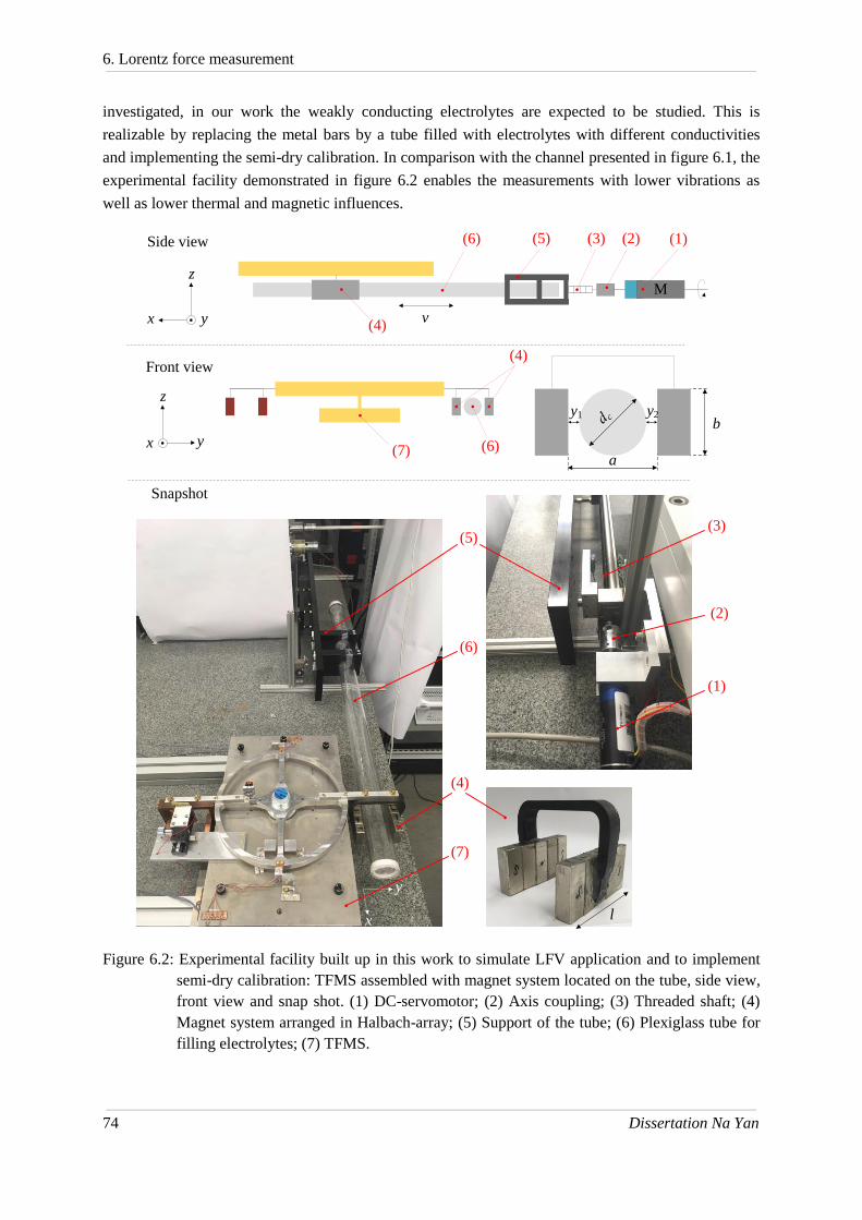
6. Lorentz force measurement
74 Dissertation Na Yan
investigated, in our work the weakly conducting electrolytes are expected to be studied. This is
realizable by replacing the metal bars by a tube filled with electrolytes with different conductivities
and implementing the semi-dry calibration. In comparison with the channel presented in figure 6.1, the
experimental facility demonstrated in figure 6.2 enables the measurements with lower vibrations as
well as lower thermal and magnetic influences.
Figure 6.2: Experimental facility built up in this work to simulate LFV application and to implement
semi-dry calibration: TFMS assembled with magnet system located on the tube, side view,
front view and snap shot. (1) DC-servomotor; (2) Axis coupling; (3) Threaded shaft; (4)
Magnet system arranged in Halbach-array; (5) Support of the tube; (6) Plexiglass tube for
filling electrolytes; (7) TFMS.
M
(1)(2)(6)
(4)v
Side view
Front view
Snapshot
(6)(7)
(3)
a
b
l
y1 y2
(4)
(5)
z
x y
z
yx
(5)
(4)
(6)
(3)
(2)
(1)
y
x
(7)

6. Lorentz force measurement
Dissertation Na Yan 75
A commercial plexiglass tube (6) with 1000 mm length, inner diameter of 46 mm and outer diameter
d = 50 mm, is situated symmetrically within the magnet system with y1 = y2 = 3 mm. The tube is
connected by the support (5) to a threaded shaft (3) which is driven by the DC-motor (1) [59]. As the
DC-motor operates, the rotation motion is transferred into the linear motion by the threaded shaft. The
tube, together with liquid inside, moves through the magnetic field simulating the flow in the channel.
The support is manufactured from polyamide and screws and nuts used for connections are made of
brass and aluminum as non-magnetic materials for minimizing the influences caused by magnetic
interaction. Because the metal shaft and screws are also electrically conductive, which could lead to
Lorentz force during the movement, the test channel is so assembled and located, that the screws,
threaded shaft and DC-motor are far from the TFMS.
The speed of the tube is controllable by giving parameters to the DC-motor. The salt water as a
mixture of tap water and sodium chloride is chosen as the electrolyte in the channel for experimental
convenience. The conductivity is also adjustable by adjusting the concentration of the salt water. This
experimental facility is flexible to provide the various values of conductivity and velocity, and is able
to contribute into the so-called semi-dry calibration to determine the measuring sensitivity of the
TFMS as a Lorentz force flowmeter.
6.2 Semi-dry calibration of the TFMS
Practical measurements with electrolytes are implemented using the experimental facility presented in
figure 6.2. Limited by the specification of the DC-motor and the pitch of the threaded shaft, the speed
of the tube is up to 3.3 mm s-1
available. The TFMS operates in the closed-loop operation mode with
electrostatic force as the compensation force. Reference measurements are initially implemented
without liquid inside the tube, signal from the TFMS is recorded with moveable empty tube as the 'dry
part' of the semi-dry calibration to determine the noises caused by the experimental facility. Then, the
same experimental procedures are carried out with the same tube filled with electrolytes. The semi-dry
calibration indicates that instead of pumping the liquid running in the channel-loop, the calibration
procedure is performed with the tube and the liquid inside moving together using the moving
mechanism.
Different electrolytes are made with salt dissolved into the tap water to achieve different concentration
presented in table 6.1. The conductivity of the empty tube is described by the conductivity of air, while
the conductivity of the tap water is measured by the conductivity meter. According to the conductivity
ordering guide [60], the conductivity of the salt water can be calculated from its concentration. The
uncertainties given in the value of conductivity are due to a maximum permissible deviation of
± 100 mg in the weight of the dissolved salt, which could be caused during weighing process and
dissolving process. Velocity values are adjusted as v = 1.2, 2.6 and 3.3 mm s-1
by sending different
values to the controller of the motor. As introduced in the section 5.5, the NPI is applied during the
data evaluation. Therefore, in order to estimate the drift signals, before and after each velocity level is
the period of standstill, namely v = 0. Considering the settling time of the TFMS in its closed-loop
operation mode and the settling time of the DC-motor, each step with the non-zero velocity lasts
30 seconds. As presented in the figure 6.3(a), before and after the motion is 300 seconds motionless
period. The movement of the tube processes forth and back alternatively with positive and negative

6. Lorentz force measurement
76 Dissertation Na Yan
velocity values, the maximum distance of the movement is thereby 99 mm (30 seconds with velocity
of 3.3 mm s-1
), which is within the stroke of the shaft, and the required space of the experimental
facility is thereby reduced.
Figure 6.3: Overview of the measured force using the semi-dry calibration. (a) Moving velocity of the
tube; (b) Recorded force values during measurement with the empty tube; (c) Recorded
force values during measurement with tube filled with electrolyte (conductivity is
4.86 S m-1
); (d) Determined force values using the newton's polynomial interpolation; (e)
Difference between the force signal with and without electrolyte.
Empty tube Raw data Moving average filter
Tube filled with electrolyte
Data evaluation using NPI
Data evaluation using subtraction
Raw data Moving average filter
(a)
(b)
(c)
(d)
(e)

6. Lorentz force measurement
Dissertation Na Yan 77
When no electrolyte is inside, during the motion of the empty tube, recorded force signal is presented
in figure 6.3 (b). In the raw data, noise is in the range of ± 100 nN which could be caused by the
mechanical noises such as vibration of the tube. To enable the movement of the tube, the TFMS is no
more located in the closed cover but exposed partially to the surroundings where airflow could also
influence the measurements and increase the noise. However, in the real practical conditions where the
TFMS is enclosed on the flow channel, this problem could be overcome. With the same procedure, the
force values determined with the electrolyte with conductivity of 4.86 S m-1
in the tube are illustrated
in the figure 6.3(c). After the data evaluation with the NPI, the force values determined during motion
of the empty tube as well as the tube with the electrolyte inside are presented in the figure 6.3(d). In
the further data evaluation, the Lorentz force generated by the moving electrolytes is determined by
subtracting the force signal captured during measurements with empty tube, the results are illustrated
in the figure 6.3(e).
Table 6.1: Conductivity values of the electrolytes used in the practical measurements; and the
experimentally obtained measuring sensitivity.
Electrolyte Conductivity
[S m-1
]
Obtained sensitivity
[nN s mm-1
]
Empty tube 3·10-15
~ 8·10-15
-
Tap water 0.026 0.0611
sodium chloride 30 g/L 4.86 ± 0.015
11.63 ± 2.88 (k = 2)
sodium chloride 100 g/L 14 ± 0.012
33.77 ± 2.4 (k = 2)
sodium chloride 167 g/L 20.4 ± 0.007 48.06 ± 3.1 (k = 2)
The same data evaluation is implemented with all the measured data in respect to the electrolytes with
different conductivities. In figure 6.4, the measured force values are presented in accordance with the
velocity values for different electrolytes. As motioned above, with the channel presented in figure 6.1,
the flow velocity of approximately of 3 m s-1
is achievable by using the pump. The available motion
speed of the tube in our work is limited by 3.3 mm s-1
, which is approximately three orders of
magnitude lower. Based on the equation (1.1), the induced Lorentz force is thereby also three orders of
magnitude lower when the electrical conductivity remains as the same. Therefore, the relationship
between the velocity and the induced force by the tap water with electrical conductivity of 0.026 S m-1
is difficult to identify. However, in the measurements on electrolytes with conductivity of 4.86 S m-1
,
14 S m-1
and 20.4 S m-1
, a good linearity can be observed. The linear fitting describing the sensitivity
ST of the TFMS as a flowmeter is applied on the measured data. The slopes of the linear fitting are
presented in the figure 6.5 and table 6.1, giving the sensitivity of the velocity measurement for
different conducting electrolytes. The sensitivity of the tap water is obtained on the linear fitting as
ST| Tap water = 0.0611 nN s mm-1
; with the velocity increased to 1 m s-1
, the corresponded force of

6. Lorentz force measurement
78 Dissertation Na Yan
Sensitivity of tap water
61.1 nN is expected to be measured. The uncertainties in the obtained sensitivities shown in figure 6.5
are from the repeatability of the force measurements. In the datasheet of the DC motor no uncertainty
is given for its rotational speed, moreover, the uncertainty of the pitch of the shaft is also unknown.
Therefore, the uncertainty of the velocity is assumed here with a relative uncertainty of 5 %. The
uncertainty in the obtained sensitivity of the TFMS for measuring velocity is determined with the
equation (6.1) and (6.2).
LT
dFS
dv (6.1)
2 2
( ) ( )T L
T TS F v
L
S Su u u
F v
(6.2)
In this measurement, the uncertainty in the obtained sensitivity ST is up to 24%, which is mainly
contributed by the measured force values. As mentioned before, in order to enable the movement of
the tube, the TFMS is difficult to be isolated from the surroundings, where influence of the airflow as
well as the vibration of mechanical structure is unavoidable, and the measurement uncertainty is
thereby increased. Another cause could be in the data evaluation using the NPI, where the estimated
drift value could be deviated from the real value. To reduce this deviation, more given data should be
used to calculate the polynomial fitting.
Figure 6.4: Determined force values in accordance Figure 6.5: Sensitivity of the TFMS working
with the velocity values for different con- as flowmeter in accordance with
ductivities. different conductivity values.
In comparison with the results achieved in work [29], with the same velocity and conductivity, the
induced Lorentz force in our work is approximately 40% lower. The reason is that in this work a
cylindrical tube with inner diameter of 46 mm is used, while in [29] the channel presented in figure 6.1
is rectangular with the inner section of 50 mm x 50 mm. The larger cross section leads to the larger
volumetric flow rate and Lorentz force is thereby with higher magnitude. Moreover, the magnetic flux

6. Lorentz force measurement
Dissertation Na Yan 79
density of the magnet system is inhomogeneous in the y-direction, which also leads to the difference in
the induced Lorentz force when the shape of the channel is different. From both figure 6.4 and 6.5, it
is indicated that the induced Lorentz force depends linearly on the velocity and the conductivity of the
electrolyte as introduced in the section 1.1. The TFMS shows a good capability to measure the Lorentz
force. Moreover, with the limited moving velocity up to 3.3 mm s-1
, the TFMS enables the force
measurement on electrolyte with conductivity of 4.86 S m-1
. The experimental data presents the
potential of the TFMS to measure with further extended range of conductivity down to 0.0064 S m-1
when the velocity is increased to 2.5 m s-1
, which is as an improvement from 0.059 S m-1
achieved in
[29] with the similar velocity value. In comparison with the DFMS, the characteristics of the TFMS
achieved in our work are presented in table 6.2.
Table 6.2: The TFMS as the newly developed force measurement system for LFV, in comparison with
the previously developed differential force measurement system (DFMS).
DFMS TFMS
Force resolution 20 nN 2 nN
Settling time 1.4 s 9.2 s
(in closed-loop)
Compensation force EMF EMF / ESF
Dead load
capacity
Approximately 1 kg;
theoretically up to 3 kg [27]
Over 3 kg;
theoretically up to 10 kg [37]
Lorentz force
measurement for
electrolyte with
conductivity down to:
0.059 S m-1
with velocity up to 2.5 m s-1
0.0064 S m-1
with velocity 2.5 m s-1
(estimated from experimental data)
6.3 Summary
In this chapter, the practical measurements were implemented. Without pumping the liquid inside the
channel, the semi-dry calibration is carried out with the experimental facility consisting of a plexiglass
tube and a moving mechanism driven by a DC-motor. Different values of moving velocity as well as
electrical conductivity were set in the measurement procedure. Because the velocity is limited up to
3.3 mm s-1
due to the moving mechanism, the conductivity is chosen as σ = [4.86, 14, 20.4] S m-1
in

6. Lorentz force measurement
80 Dissertation Na Yan
our work, higher than that used in previous research [29], in order to achieve the Lorentz force in the
range of nanonewton. During the measurement, procedures with and without motion were processed
alternately with different duration to estimate and compensate the drift using the NPI in the data
evaluation. In the measurement results, a good linear relationship between the induced force and the
velocity as well as conductivity was indicated. The sensitivity of the TFMS to measure the velocity
was obtained using the semi-dry calibration in respect to different conductivity values.
To summarize with table 6.2, for horizontal force measurement, the TFMS achieved a resolution of
2 nN by using NPI in the data evaluation. Moreover, the dead load capacity is improved to 3 kg
(theoretically up to 10 kg due to the maximum load capacity of the flexible bearing). The dynamic
behavior with the settling time of 9.2 s is also acceptable for the LFV application. According to the
practical measurements on electrolytes, the TFMS enables force measurement for electrical con-
ductivity of 4.86 S m-1
. When the velocity is increased from 3.3 mm s-1
to 2.5 m s-1
as the velocity that
was arranged for measurements with DFMS, the TFMS shows the potential to implement
measurements with even lower conductivity down to 0.0064 S m-1
, which is a great improvement
compared to 0.059 S m-1
achieved in [29].

7. Conclusions and Outlook
Dissertation Na Yan 81
7. Conclusions and Outlook
The presented work aims to develop a high resolution force measurement system to contribute to the
Lorentz force velocimetry application for velocity measurement of weakly conducting electrolytes.
Initially, the EMFC weighing cell as the core component of the previously developed FMSs is
investigated. In previous work, the EMFC weighing cell was located in the suspended configuration
carrying the 1 kg magnet system as the dead load, differing from its common usage as the balance. To
study how the configurations and dead load values influence the measurement of the EMFC, the tilt
sensitivity contributing to the measurement uncertainty and the stiffness determining the measuring
sensitivity were tested in chapter 2. Experiments were carried out with the EMFC located on a tilt
stage in four different configurations, and with different dead load values. The following points are
concluded from chapter 2:
To measure horizontally directed forces, the weighing cell in its sidewise configuration,
suspended configuration with weighing pan upwards and with weighing pan downwards
(figure 2.2) can be arranged. In each of the three configurations, linear relationship between
the tilt sensitivity and the applied dead load was revealed;
With the obtained linear relationship, the dead load value is determined, by which the tilt
sensitivity was found to be zero. Therefore, a tilt-insensitive system can be theoretically
achieved. In this way, the measurement uncertainty can be reduced (figure 2.5);
In different configurations of the EMFC weighing cell, the stiffness of the system is
different. Moreover, during the sidewise configuration, the stiffness is constant to the
applied dead load values, while in the other three configurations the stiffness is further
changed by changing dead loads (figure 2.9), which leads to the change in the measuring
sensitivity of the system.
Although compensation weight can be manually applied to the EMFC weighing cell to achieve an
insensitive system to the unavoidable tilt angles, with the necessity to carry the 1 kg magnet system, it
is not generally desirable to apply the counterweight at such an order of magnitude on the precise
mechanical structure of the weighing cell. Additionally, the stiffness of the EMFC is further increased
by supporting the 1 kg magnet in the suspended configuration in work [27, 29], which makes the FMS
less sensitive.
Considering the stiffness of the system is insensitive to the dead load in its sidewise configuration, as a
transformation from the EMFC weighing cell in its sidewise configuration, the torsion force
measurement system based on the principle of torsion balance was introduced in chapter 3. In the
theoretical design concept, the symmetrical plane wheel carries the magnet system on one side and a
non-magnetic dummy with a similar weight and geometrical parameters on the other side. A
commercial flexible bearing hinge supports the plane wheel, enabling the rotation motion without
friction and providing the elastic force balancing the external force. Rotation motion is detected by the
optical positioning sensor with a compact size and providing sufficient resolution of 1 nm. Initial idea

7. Conclusions and Outlook
82 Dissertation Na Yan
of developing the torsion force measurement system is that the symmetrical geometry provides the
equal arm lengths LT1 and LT2, and with the similar weight of the dead load (magnet system and
dummy) on each side, the precondition of a tilt-insensitive system is reached without applying
additional compensation dead load in high magnitude. Theoretical calculations were made to design
the system considering the following points:
The geometrical parameters;
The spring constant and maximum axial load of the flexible bearing given by the manufacturer;
The resolution of the positioning sensor;
The target force resolution of 2 nN.
By using a flexible bearing with the spring constant of 1.17·10-2
N m rad
-1 (value given by
manufacturer) and LT1 = LT2 = 180 mm, R as the distance from the positioning sensor to the rotational
axis is 135 mm, the stiffness of the system is 0.48 N m-1
and thereby the force resolution of 0.48 nN is
calculated based on the theoretical calculations.
In chapter 4, the deflection method as a traceable method to perform the position calibration as well as
force calibration was introduced by utilizing the tilt dependency of the system. Traceable tilt force
caused by the tilt angle and standard mass piece was considered as the reference actuation force on the
TFMS, by which the electrical voltage as the initial output of the positioning sensor was calibrated
into rotational angles with the calibration factor Kps = 0.4207 ± 0.0012 mrad V-1
(k = 2), as well as into
force values with KF = 30.07 ± 0.23 µN V-1
(k = 2). Because of the low stiffness and the high dead
load, the natural frequency of the TFMS is low (0.06 Hz); and as an underdamped system with the
damping ration of 0.0163, the cutoff frequency is as low as 0.002 Hz. The dynamic behavior is
expected to be improved by setting up the closed-loop operation mode.
In chapter 5, the closed-loop operation mode was build up based on the PID-controller, where the
force signal is no longer calculated from the voltage value using the force calibration factor KF, but
described by the compensation force which brings the deflection of the TFMS continuously back to
the null position. The TFMS in its closed-loop operation mode was tested with the electromagnetic
force as the compensation force provided by a commercial voice coil actuator. Then, a customized
electrostatic force generator based on the structure of plate-shaped capacitor was introduced. Taking
the whole TFMS as one conductor, a customized capacitor is built by assembling a PCB plate near the
TFMS as the second electrode. Electrostatic force was generated between the two electrodes while
actuation voltage is applied across them. Additionally, the calibration of the electrostatic force was
implemented by using the following three methods (figure 5.6), they are:
(a) By measuring the capacitance values with different distances between the two electrodes as
a way to determine the capacitance gradient;
(b) By comparing the electrostatic force with the electromagnetic force, which is calibrated
using the deflection method and works as the reference force;
(c) By setting the TFMS in a velocity mode, the calibration factor can be determined by
measuring the induced current in the capacitor.
An agreement was presented by using the three calibration methods. With the lower uncertainty as
well as minimal deviation from the theoretical calculation, the calibration factor determined by method

7. Conclusions and Outlook
Dissertation Na Yan 83
(a) is taken for further measurements. The customized capacitive actuator presented the ability to be
used as a force generator. In the test of the dynamic behavior, the TFMS was tested in the open-loop
and closed-loop with electromagnetic force as well as electrostatic force as the compensation force
respectively. The dynamic behavior was improved as the cutoff frequency is increased to 0.1 Hz.
Additionally, the electrostatic force operated at the same level as the electromagnetic force in the
compensation procedure. As summarized in section 5.6, the customized capacitive actuator is a
reasonable replacement of the commercial voice coil actuator with the following improvements:
(1) More suitable for the LFV application where magnet system is involved;
(2) No power wires connected to the rotational part of the TFMS;
(3) Force constant Kes with lower relative uncertainty;
(4) Force constant Kes can be adjusted by changing the geometry of the capacitor.
In the test of the force resolution, the newton's polynomial interpolation is introduced in the data
evaluation to estimate and compensate the thermal and seismic drift and noises; the force down to
2 nN is resolved.
Lastly, the TFMS was involved in the Lorentz force measurement. The semi-dry calibration was
introduced by using a tube to simulate the channel. With the liquid inside moving together with the
tube driven by the moving mechanism, the flow channel is simulated with lower vibrations. In this
experiment, the TFMS shows the good feasibility to measure the Lorentz force, which is linearly
proportional to the velocity and conductivity. With a limited velocity up to 3.3 mm s-1
, the Lorentz
force is measurable on electrolyte with conductivity down to 4.86 S m-1
. This shows the potential to
extend the measurement range further down to 0.0064 S m-1
when the velocity is increased to 2.5 m s-1
,
indicating the velocity arranged in work [29], where measurements on electrolytes with conductivity
down to 0.059 S m-1
were achieved by the DFMS.
To conclude, as a newly developed FMS to measure the induced Lorentz force by weakly conducting
electrolytes, the TFMS shows good capabilities with improved resolution, increased load capacity and
multiple possibilities to perform actuation and compensation forces (table 6.2). Moreover, with easily
commercially achieved components (flexible bearing, voice coil actuator, positioning sensor) and
several customized components (PCB and capacitive actuator), the cost of the TFMS is also a great
advantage compared to the EMFC weighing cell.
As mentioned in section 5.6, one of the future tasks is setting up the differential capacitive force
actuator, with which the measuring range of the TFMS can be increased and the pre-voltage in the
PID-controller is no more necessary.
Concerning that the semi-dry calibration was performed with limited velocity up to 3.3 mm s-1
in our
work, the moving mechanism will be improved with the aim to increase the achievable moving
velocity. This improvement can be based on changing the DC-motor and using a threaded shaft with
larger pitch. However, because the motion period lasts 30 seconds during the measurement (figure 6.3),
the velocity up to approximately 33 mm s-1
is thereby limited while implementing the semi-dry
calibration on the tube with the limited length of 1000 mm. To overcome this limitation, the linear
moving mechanism will be replaced by the rotating mechanism presented in figure 7.1, where the
1000 mm-long tube is replaced by an annular pipe. Similar to the tube presented in figure 6.2, the

7. Conclusions and Outlook
84 Dissertation Na Yan
annular pipe is filled with electrolytes and moves through the magnetic field. Moreover, the annular
pipe is able to rotate continuously without considering the limitation of the stroke. Higher velocity
values in the range of several meters per second can be thereby achieved, the velocity is dependent on
the specifications of the motor, the dead load supported by the motor and also the diameter of the
annular pipe (Da in figure 7.1). With the new experimental facility, the semi-dry calibration can be
implemented on electrolytes with further lower conductivity. Additionally, in order to reduce the
environmental noise, a shell will be manufactured for the TFMS to improve the isolation from
surroundings.
The second generation of the TFMS has already been developed and manufactured with a reduced
geometry (270 mm x 45 mm x 60 mm). As another task in the further, the new TFMS will work
together with the bulk superconductor as magnet system under cryogenic isothermal condition in a
cryostat, with which high magnetic flux density is expected to be achieved. The feasibility to measure
the Lorentz force using the second generation of the TFMS will also be tested on the experimental
facility presented in figures 6.2 and 7.1.
Figure 7.1: Replacement experimental facility with annular pipe to carry out semi-dry calibration.
(1) Annular pipe; (2) Magnet system; (3) TFMS.
v
Side view
Front view (cross section)
(1)(3)
(2)
z
x y
z
yx
(1)
(2)
(3)

Appendix
Dissertation Na Yan 85
Appendix A Calibration of the NI9239
Figure A1: Calibration of the NI voltage module according to the reference voltage values provided by
multi-function calibrator. Stepwise signals are generated in the range of ± 10 V (left, blue)
and ± 1 V (right, red). At each step 9000 values are recorded during 30 minutes, from
which the mean value and the uncertainty of the voltage step are determined. Then as
shown in the two bottom figures, the mean value of the uncertainties of all the steps is
calculated as 9.24 µV for each of the two measuring ranges.
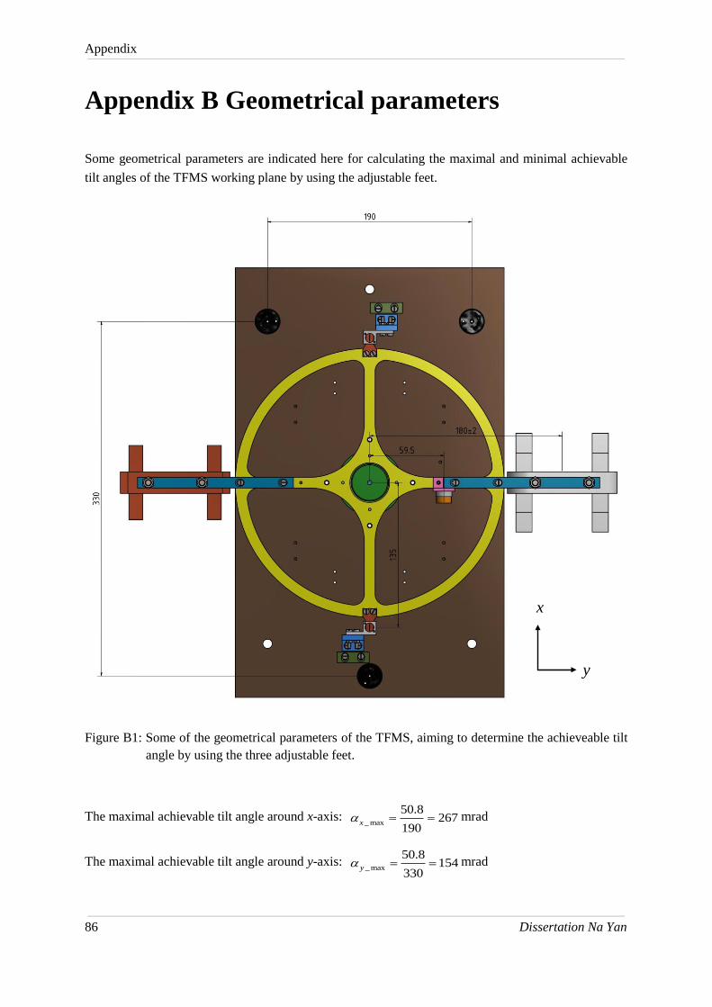
Appendix
86 Dissertation Na Yan
Appendix B Geometrical parameters
Some geometrical parameters are indicated here for calculating the maximal and minimal achievable
tilt angles of the TFMS working plane by using the adjustable feet.
Figure B1: Some of the geometrical parameters of the TFMS, aiming to determine the achieveable tilt
angle by using the three adjustable feet.
The maximal achievable tilt angle around x-axis: _ max
50.8267
190x mrad
The maximal achievable tilt angle around y-axis: _ max
50.8154
330y mrad
x
y

Appendix
Dissertation Na Yan 87
Due to a full turn of the fine screws:
The minimal achievable tilt angle around x-axis: _ min
0.251.32
190x mrad
The minimal achievable tilt angle around y-axis: _ min
0.250.76
330y mrad
Further smaller tilt angles are achievable by turning the screws by 1/2 turn and 1/4 turn.
Bibliography
88 Na Yan Dissertation
Bibliography
[1] A. Thess, E. Votyakov, Y. Kolesnikov. Lorentz Force Velocimetry. Phys. Rev. Lett, 96 164501,
2006.
[2] Y. Kolesnikov, C. Karcher, A. Thess. Lorentz force flowmeter for liquid aluminum: Laboratory
experiments and plant tests. Metallurgical and Materials Transactions B, 42(3):441–450, 2011.
[3] A. Wegfrass, C. Diethold, M. Werner, C. Resagk, T. Fröhlich, B. Halbedel, A.Thess. Flow rate
measurement of weakly conducting fluids using Lorentz force velocimetry. Measurement Science
and Technology, 23(10):105307, 2012.
[4] C. Weidermann. Design and laboratory test of a Lorentz force flowmeter for pipe flows. PhD
thesis, Technical University of Ilmenau, 2013.
[5] C. Heinicke, A. Thess. Electromagnetic force on a magnetic dipole inside an annular pipe flow.
Physics of Fluids, 25(9), 2013.
[6] C. Heinicke, A. Thess, I. Rahneberg. Towards local resolution measurements in turbulent liquid
metal duct flows. Journal of Physics: Conference Series, 318(7):072029, 2011.
[7] B. Halbedel, C. Resagk, A. Wegfrass, C. Diethold, M. Werner, F. Hilbrunner, A. Thess. A novel
contactless flow rate measurement device for weakly conducting fluids based on Lorentz force
velocimetry. Flow, Turbulence and Combustion, 92(1-2):361–369, 2014.
[8] A. Wegfrass, C. Diethold, M. Werner, T. Fröhlich, B. Halbedel, F. Hilbrunner, C. Resagk, A.Thess.
A universal noncontact flowmeter for liquids. Applied Physics Letters, 100, 194103, 2012.
[9] B. Hartmut, K. Porzig, J. Mengelkamp, M. Carlstedt, M. Ziolkowski, H. Toepfer. Lorentz force
eddy current testing: a novel nde-technique. COMPEL- The international journal for computation
and mathematics in electrical and electronic engineering, 33(6):1965–1977, 2014.
[10] M. Werner. Design, Optimierung, Realisierung und Test von passive Magnetsystemen für die
Lorentzkraftanemometrie an Electrolyten. PhD thesis, Technical University of Ilmenau, 2013.
[11] I. Sokolov, Y. Kolesnikov, A. Thess. Experimental investigation of the transient phase of the
lorentz force response to the time-dependent velocity at finite magnetic Reynolds number.
Measurement Science and Technology. 25(12):125304, 2014.
[12] J. R. Pratt, J. A. Kramar, D. B. Newell, D. T. Smith. Review of SI traceable force metrology for
instrumented indentation and atomic force microscopy. Measurement Science and Technology.
16 2129–2137, 2005.

Bibliography
Dissertation Na Yan 89
[13] D. B. Newell, J. A. Kramar, J. R. Pratt, D. T. Smith, E. R. Williams. The NIST Microforce
Realization and Measurement Project. IEEE Transactions on Instrumentation and Measurement,
52:508, 2003.
[14] G. A. Shaw, J. Stirling, J. A. Kramar, A. Moses, P. Abbott, R. Steiner, A. Koffman, J. R. Pratt , Z.
J. Kubarych. Milligram mass metrology using an electrostatic force balance. Metrologia, 53
A86-A94, 2016.
[15] R. Leach, D. Chetwynd, L. Blunt, J. Haycocks, P. Harris, K. Jackson, S. Oldfield, S. Reilly.
Recent advances in traceable nanoscale dimension and force metrology in the UK. Measurement
Science and Technology, 17 467-476, 2006.
[16] J Stirling, G. A. Shaw. Realising traceable electrostatic forces despite non-linear balance motion.
Measurement Science and Technology, 28-055003, 2017.
[17] M. Kim, J. R. Pratt, U. Brand, C. W. Jones. Report on the first international comparison of small
force facilities: a pilot study at the micronewton level. Metrologia, 49-1, 2011.
[18] L. Song, Y. Zheng, G. Hu, J. Ma, T. Werner, M. Zhao, F. Fang. Highly sensitive, precise, and
traceable measurement of force. Instrumentation Science and Technology. 44, NO.4,386-400,
2016.
[19] C. Diethold, M. Kühnel, T. Ivanov, I. W. Rangelow. T. Fröhlich. Determination of AFM-
Cantilever spring constants using the TU Ilmenau force displacement measurement device. In
Proceedings of the XXI IMEKO world Congress, S.175-180, 2015.
[20] M. Kühnel, M. Rivero, C. Diethold, T. Fröhlich. Precise tiltmeter and inclinometer based on
commercial force compensation weigh cells. In Proceedings of IMEKO International TC3, TC5
& TC22 Conference, 2014.
[21] T. Quinn, C. Speake, H. Parks, R. Davis. The BIPM measurements of the Newtonian constant of
gravitation, G. Philosophical Transactions of the Royal Society A, 372:2014032, 2014.
[22] S. J. Chen, S. S. Pan. Nanonewton Force Generation and Detection Based on a Sensitive Torsion
Pendulum. IEEE Transactions on Instrumentation and Measurement, 58-4, 2009.
[23] T. A. Wagner. Rotating Torsion Balance Tests of the Weak Equivalence Principle. PhD thesis,
University of Washington, 2014.
[24] S. Schlamminger. Determination of the Gravitational Constant using a Beam Balance, PhD thesis,
University of Zürich, 2002.
[25] H. V. Parks, J. E. Faller. Simple Pendulum Determination of the Gravitational Constant. Physical
Review Letters, 105, 110801, 2010.
[26] V. Nesterov, M. Mueller, L.L. Frumin, U. Brand. A new facility to realize a nanonewton force
standard based on electrostatic methods. Metrologia, 46 277-282, 2009.
Bibliography
90 Na Yan Dissertation
[27] C. Diethold. Lorentzkraft-Anemonetrie von elektrisch schwach leitfähigen Fluiden. PhD thesis,
Technical University of Ilmenau, 2015.
[28] P. Sun, M. Zhao, J. Jiang, Y. Zheng, Y. Han and L. Song. The Differential Method for Force
Measurement Based on Electrostatic Force. Journal of Sensors, 1857920, 2017.
[29] S. Vasilyan. High Precision Force Measurements in Horizontal Direction in Combination with
High Dead Loads: Non-contact Flowmeter for Low Conducting Electrolytes. PhD thesis,
Technical University of Ilmenau, 2015.
[30] S. Vasilyan, M. Rivero, J. Schleichert, B. Halbedel, T. Fröhlich. High-precision horizontally
directed force measurements for high dead loads based on a differential electromagnetic force
compensation system. Measurement Science and Technology, 27-045107, 2016.
[31] S. Vasilyan, R. Ebert, M. Weidner, M. Rivero, B. Halbedel, C. Resagk, T. Fröhlich. Towards
metering tap water by Lorentz force velocimetry. Measurement Science and Technology, 26-
115302, 2015.
[32] S. Vasilyan, T. Fröhlich. Direct Lorentz force compensation flowmeter for electrolytes. Applied
Physics Letters, 105,223410, 2014.
[33] M. Kühnel, M. Rivero, C. Diethold, F. Hilbrunner, T. Fröhlich. Dual axis tiltmeter with nano
resolution based on commercial force compensation weigh cells. In Proceedings of 58th Ilmenau
Scientific Colloquium, 2014.
[34] N. Yan, S. Vasilyan, M. Kühnel, T. Fröhlich. Investigation to the tilt sensitivity of the
Lorentz force velocimetry system for the flow rate measurement of low conducting fluids.
In Proceeding of IMEKO TC3, TC5 and TC22 Conferences, 2017.
[35] M. Rivero, M. Kühnel, T. Fröhlich. High precision dual axis tilt stage. In Proceedings of 58th
Ilmenau Scientific Colloquium, 2014.
[36] H. Cavendish. Experiments to determine the Density of the Earth. Phil. Trans. R. Soc. Lond, vol.
88 469-526, 1798.
[37] C-Flex Bearing. Design Guide: https://c-flex.com/pivot-bearings/design-guide/ (accessed 29. Oct.
2018).
[38] C. Diethold, T. Fröhlich, F. Hilbrunner, G. Jäger. High precision optical position sensor for
electromagnetic force compensated balances. In Proceeding of IMEKO TC3, TC5 and TC22
Conferences, 2010.
[39] Datasheet analoge input module NI9239: http://www.ni.com/pdf/manuals/375939b_02.pdf
(accessed 29. Oct. 2018).
[40] Haag-Streit AG, Elcomat 3000: https://www.haag-streit.com/de/moeller-wedel-
optical/produkte/elektronische-autokollimatoren/elcomat-reihe/elcomat-3000/ (accessed 29. Oct.
2018).

Bibliography
Dissertation Na Yan 91
[41] N.Yan, M. Kühnel, S. Vasilyan, T. Fröhlich. Torsion balance-based system for high-
precision force measurement in horizontal plane; part I. Development concept.
Measurement Science and Technology, 29 084001, 2018.
[42] Organisation Internationale de Métrologie Légale 2004 Weights of classes E1, E2, F1, F2, M1, M1–2,
M2, M2–3 and M3, Internal Recommendation OIML R111-1
[43] Result of the absolute gravitational acceleration measurement at the Technical University of
Ilmenau.
[44] N Yan, M. Kühnel, S. Vasilyan, T. Fröhlich. Calibration of the torsion force measurement
system for the Lorentz force velocimetry application. In Proceedings of 59th
Ilmenau
Scientific Colloquium, 2017.
[45] Datasheet linear voice coil motor: http://moticont.com/pdf/lvcm-016-010-01.pdf (accessed 29.
Oct. 2018).
[46] Datasheet Universal source 3245A: http://www.testequipmenthq.com/datasheets/Agilent-3245A-
Datasheet.pdf (accessed 29. Oct. 2018).
[47] C. Diethold, F. Hilbrunner. Force measurement of low forces in combination with high dead
loads by the use of electromagnetic force compensation. Measurement Science and Technology,
23 074017, 2012.
[48] O V. Vakaliuk, M D. Ainslie, B. Halbedel. Lorentz force velocimetry using a bulk HTC magnet
system: proof-of-concept. Supercond. Sci. Technol. 31 084003. 2018.
[49] Data sheet HIOKI Impendance analyzer IM3570:
https://www.hioki.com/file/cmw/hdCatalog/4765/pdf/?action=browser&log=1&lang=en
(accessed 29. Oct. 2018).
[50] F. Hilbrunner, I. Rahneberg, T.Fröhlich. Wattwaage mit Hebelübersetzung auf Basis eines
kommerziellen EMK-Wägesystems.Technisches Messen,2196-7113, 2017.
[51] J. Lunze. Regelungstechnik 1. Springer Vieweg, ISBN 978-3-642-29533-1, 2014.
[52] S. Davidson, M. Perkin, M. Buckley. The Measurement of Mass and Weight. Measurement Good
Practice Guide No.71. 2004.
[53] Hamming R.W. Numerical Methods for Scientist and Engineers Dover Publications. Inc., New
York, ISBN 0-486-65241-6, 1962.
[54] Y. Zheng, M. Zhao, P. Sun, L. Song. Optimization of Electrostatic Force System Based on
Newton Interpolation Method. Journal of Sensors. Article ID 7801597, 2018
[55] S. Chen, S Pan. A force measurement system based on an electrostatic sensing and actuating
technique for calibrating force in a micronewton range with a resolution of nanonewton scale.
Measurement Science and Technology, 22 045104, 2012.

Bibliography
92 Na Yan Dissertation
[56] A. Wegfraß. Experimentelle Untersuchungen zur Anwendbarkeit der Lorentzkraft-Anemometrie
auf schwach leitfähige Fluid. PhD thesis, Technical University of Ilmenau, 2013.
[57] THORLABS fine Hex Adjuster:
https://www.thorlabs.com/newgrouppage9.cfm?objectgroup_id=1205 (accessed 29. Oct. 2018).
[58] V. Minchenya, C. Karcher, Y. Kolesnikov, A. Thess. Dry calibration of the Lorentz force
flowmeter. Magnetohydrodynamics Vol.45. pp 569-578, 2009.
[59] Datasheet Brushless DC-Servomotor:
https://www.faulhaber.com/fileadmin/Import/Media/EN_3056_B_FMM.pdf (accessed 29. Oct.
2018).
[60] Conductivity ordering guide:
http://myweb.wit.edu/sandinic/research/conductivity%20v%20concentration.pdf (accessed 29.
Oct. 2018).

Erklärung
Dissertation Na Yan 93
Erklärung
Ich versichere, dass ich die vorliegende Arbeit ohne unzulässige Hilfe Dritter und ohne Benutzung
anderer als der angegebenen Hilfsmittel angefertigt habe. Die aus anderen Quellen direkt oder indirekt
übernommenen Daten und Konzepte sind unter Angabe der Quelle gekennzeichnet.
Bei der Auswahl und Auswertung folgenden Materials haben mir die nachstehend auf-
geführten Personen in der jeweils beschriebenen Weise unentgeltlich geholfen:
Prof. Dr.-Ing. habil. Thomas Fröhlich --- Fachliche Betreuung während der Promotionszeit.
Dr.-Ing. Suren Vasilyan --- Vorstellung des FMSs und Strömungskanals (entwickelt und
verwendet von den ersten und zweiten Generationen des Projektes Lorentz Force Velocimetry
and Lorentz Force Eddy Current Testing) im Jahr 2016 beim Beginn dieser Arbeit.
M. Sc. Ivan Horodyskyi --- Studentische Hilfskraft: Durchführung der Messungen in
Abschnitten 4.1 und 4.2.
Frau Mengchen Yan --- Sprachkorrektur; Ausschließlich Bearbeitung von Rechtschreibung
und Grammatik. Es wurden keine inhaltlichen Änderungen, Ergänzungen oder weitere
Beiträge durch sie vorgenommen
Weitere Personen waren an der inhaltlich-materiellen Erstellung der vorliegenden Arbeit nicht
beteiligt. Insbesondere habe ich hierfür nicht die entgeltliche Hilfe von Vermittlungs- bzw.
Beratungsdiensten (Promotionsberater oder anderer Personen) in Anspruch genommen. Niemand hat
von mir unmittelbar oder mittelbar geldwerte Leistungen für Arbeiten erhalten, die im Zusammenhang
mit dem Inhalt der vorgelegten Dissertation stehen.
Die Arbeit wurde bisher weder im In- noch im Ausland in gleicher oder ähnlicher Form einer
Prüfungsbehörde vorgelegt.
Ich bin darauf hingewiesen worden, dass die Unrichtigkeit der vorstehenden Erklärung als
Täuschungsversuch bewertet wird und gemäß § 7 Abs. 10 der Promotionsordnung den Abbruch des
Promotionsverfahrens zur Folge hat
Ilmenau, 05.11.2018 Na Yan