high quality modal testing methods - Imperial College London
272
IMPERIAL COLLEDGE OF SCIENCE, TECHNOLOGY AND MEDICINE University of London HIGH QUALITY MODAL TESTING METHODS by Mohammad Reza Ashory A thesis submitted to the University of London for the degree of Doctor of Philosophy Dynamics Section Department of Mechanical Engineering Imperial College of Science, Technology and Medicine London, SW7 2BX March 1999
Transcript of high quality modal testing methods - Imperial College London

IMPERIAL COLLEDGE OF SCIENCE, TECHNOLOGY
AND MEDICINE
University of London
HIGH QUALITY MODAL TESTING
METHODS
by
Mohammad Reza Ashory
A thesis submitted to the University of London for the degree of Doctor of Philosophy
Dynamics Section Department of Mechanical Engineering
Imperial College of Science, Technology and Medicine London, SW7 2BX
March 1999

_____________________________________________________________________i
ABSTRACT
Modal Analysis has been a developing science in the experimental evaluation of the
dynamic properties of the structures. In practice, the models produced by modal
testing often have poor quality due to factors inherent in the measurement. One of the
sources of a lack of precision in modal testing is the errors caused by mechanical
devices such as accelerometers, suspension springs and stingers.
The aim of this thesis is to improve the current methods of modal testing for dealing
with mechanical errors and to develop new ones which permit the acquisition of
modal test data of high quality. To achieve this end, the work initially focuses on
reviewing existing methods. The research, then, focuses on developing methods for
assessing the quality of the measurement; and for cancelling the effects of mechanical
devices on the measured FRFs in the cases that the quality of the measurement is not
acceptable.
A new method has been developed for the correction of mass-loading effects of
accelerometers on measured FRFs. It is shown that the non-driving point FRFs can be
corrected if the measurement is repeated with an accelerometer with different mass. It
is also shown that the driving point FRF of the response point can be obtained by the
same procedure without actually having to measure it. Moreover, this method is used
for assessing the quality of the measurement due to mass-loading effects of
transducers in a conventional modal test. A similar method is developed for assessing
the quality of measurement and for the correction of the effects of suspension springs
on the measured FRFs.
The problem of the interaction between the test structure and the shaker through
stinger is discussed and the practical ways to avoid the effects of the stinger on the
measured FRFs has been investigated. Particular attention is given to the problem of
the misalignment of the stinger and its effect on the measured FRFs. Moreover, a
method for assessing the effects of the stinger on the measured FRFs is presented.

_____________________________________________________________________ii
The correction method is further developed for the cases that the test structure is
affected by mechanical elements in more than one DOF. Moreover, it is shown that
nonlinearity of the structure or the attached elements affects the results of the
correction of the measured FRFs.
Although a new trend has been developed for the initial aim of dealing with
mechanical errors in modal testing, it has been shown that this new trend is applicable
in other fields of modal testing such as generation of rotational FRFs. On this basis a
method is developed to eliminate the need for producing the rotational excitations and
measuring them.
It is also shown that the whole matrix of translational FRFs can be generated from
measurements of one column using one accelerometer and one dummy mass. This
procedure can eliminate the problem of residual effects of out-of-range modes.
Finally, a recommended test strategy for acquisition of modal test data of high quality
related to the mechanical errors is presented.

_____________________________________________________________________iii
Acknowledgements
I would like to express my gratitude to my supervisor, Prof. D. J. Ewins, for his
valuable advice, interest, and encouragement throughout this project. I also thank Mr.
D. A. Robb for his advice and discussions.
I would like to thank my past and present colleagues of Imperial College Dynamics
Section who by their enthusiasm, encouragement and their useful discussions
provided insight into related fields of interest and enjoyable working environment.
I am grateful to the ministry of culture and higher education of Iran for the financial
support provided for this project.
Special thanks are due to my mother, my wife and my daughter for all their love,
patience and support during the course of this work, especially during the last few
months. Without them this thesis would not have been completed.

Nomenclature High quality modal testing methods iv
iv
Nomenclature
Basic Terms and Dimensions
x , y , z translational DOFs (time domain)
θx , θy , θz rotational DOFs (time domain)
X , Y , Z displacements (frequency domain)
′′X acceleration (frequency domain)
ω , f frequency of vibration (in rad/sec; Hz)
P , F forces (frequency domain)
R , ′R reaction forces (frequency domain)
M moment (frequency domain)
m , m1 , m2 , … mass of an object/accelerometer
k , k1 , k2 , … stiffness of the spring
c , c1 , c2 , … damping value
ρ mass density
A cross section area
I area moment of inertia
i , j , k , l points on the structure
ε ε ε, ,1 2 values of the noise error
TR transmissiblity ratio
ksh translational stiffness of the shaker suspension
krsh rotational stiffness of the shaker suspension
msh mass of the shaker
mcl mass of the shaker coil
mst mass of the structure
Wst weight of the structure
kst stiffness of the structure suspension
kver elastic cord (suspension spring) axial stiffness
klat elastic cord (suspension spring) lateral stiffness
lo zero-load elastic cord (suspension spring) length
l f elastic cord (suspension spring) length under load

Nomenclature High quality modal testing methods v
v
Esp elastic modulus of the elastic cord
Asp cross sectional area of the elastic cord
ls length of the stinger
lmax maximum allowable length of the stinger
ds diameter of the stinger
dmin minimum allowable diameter of the stinger
σ s material endurance stress of the stinger
Es Young’s modulus of the stinger
I s area moment of inertia of the stinger
Gs shear modulus of the stinger
As shear area of the stinger
fmin minimum desirable measurement frequency
f max maximum desirable measurement frequency
ksx stinger’s axial stiffness
msxt total mass of the shaker coil, the force transducer
and the mounting hardware
ma mass of the accelerometer
md mass of the dummy mass
&&x acceleration (time domain)
fe effective force (time domain)
fmeas measured force (time domain)
mext total extra mass attached to the structure
kext total extra stiffness attached to the structure
β coefficient of the nonlinear term in Duffing’s equation
βext coefficient of the nonlinear term of a nonlinear spring
attached to the structure
Gxy cross spectrum between signals x and y
Gxx auto spectrum of signal x
H estimator
j imaginary value ( − 1 )
n number of modification DOFs

Nomenclature High quality modal testing methods vi
vi
nc number of different configurations
r number of unknowns
s spacing between accelerometers
Matrices and Vectors
[ ] matrix
{ } column vector
determinant of a matrix
norm of a matrix/vector
[ ]T; { }T
transpose of a matrix; vector
[ ]I identity matrix
[ ]−1 inverse of a matrix
[ ]+ generalised/pseudo inverse of a matrix
[ ]H complex conjugate transpose of a matrix
[ ]U , [ ]V matrices of left and right singular vectors
[ ]Σ rectangular matrix of singular values
σ i singular value i
c c11 12, ,... the elements of the inverse of a matrix
Spatial Properties
[ ]ωr2 diagonal natural frequencies matrix
[ ]ωor2 diagonal natural frequencies matrix of the modified system
[ ]M mass matrix
[ ]K stiffness matrix
[ ]C damping matrix
[ ]∆M mass modification matrix
[ ]∆K stiffness modification matrix
∆Mi the mass attached to the structure at DOF i
∆Ki the stiffness attached to the structure at DOF i
{ }x displacement vector (time domain)
{ }&&x acceleration vector (time domain)

Nomenclature High quality modal testing methods vii
vii
{ }f force vector (time domain)
Modal and Frequency Response Properties
ωr natural frequency of r th mode (rad/sec)
ωor natural frequency of r th mode of the modified system
(rad/sec)
[ ]λ r eigenvalue matrix
[ ]φ mass-normalised mode shape/eigenvector matrix
λr r th eigenvalue
{ }φr r th mode shape/eigenvector
φir i th element of r th mode shape/eigenvector
r ij ir jrA = φ φ the modal constant for mode r and DOFs i and j
[ ]α ω( ) receptance matrix
[ ]D( )ω dynamic stiffness matrix
[ ]Dmd
( )ω dynamic stiffness matrix of the modified structure
[ ]A( )ω accelerance matrix
αij individual receptance element for DOFs i and j
(response at DOF i and excitation at DOF j)
Aij individual accelerance element for DOFs i and j
AiR jR, accelerance of points i and j and in rotational DOF , here i
and j refer to the points and R refers to the rotational DOF
αijl( ) measured receptance when a mechanical element is attached
to the structure at DOF l
Aijl( ) measured accelerance when a mechanical element is attached
to the structure at DOF l
Aijl k( , ) measured accelerance when two mechanical elements are
attached to the structure at DOFs l and k
Aijl k( , ) measured accelerance when an accelerometer is attached
at DOF k and a dummy mass is attached at DOF l
αij* measured receptance of a modified structure
(more than 2 DOFs)

Nomenclature High quality modal testing methods viii
viii
Aij* measured accelerance of a modified structure
(more than 2 DOFs)
Aijl( ) , Aij
l( ) , Aijl( ) measured accelerances for different configurations
( ) ( )pij
lA measured accelerance for pth configuration
αmm , αnn , αrr the receptances of the attached mechanical elements
′α ii the receptance of the attached mechanical element at DOF i( )p
ii′α the receptance of the attached mechanical element
at DOF i for pth configuration
[ ]′αii the matrix of the receptances of the attached mechanical
elements for different configurations
αijg receptance of the grounded structure
~Aij computed FRF using uncolibrated data
$Aij computed FRF of a nonlinear system(Aij noisy FRF
E A ( )ω measured accelerance error
Abbreviations
FEM Finite Element Method
FRF(s) Frequency Response Function(s)
DOF(s) Degree(s)-of-Freedom
RDOF(s) Rotational Degree(s)-of-Freedom
FFT Fast Fourier Transform
SVD Singular Value Decomposition
dB decibel
SMURF Structural Modifications Using experimental frequency
Response Functions
PBC Perturbed Boundary Condition
ARMA Auto-Regressive Moving-Average (method/model)
UMPA Unified Matrix Polynomial Approach (method/model)
LDV Laser Doppler Vibrometer

Table of contents High quality modal testing methods ix
ix
Table of contents
Abstract i
Acknowledgement iii
Nomenclature iv
Chapter 1. Introduction
1.1 Background__________________________________________________________1
1.2 Finite Element Method (FEM) __________________________________________2
1.3 Modal testing method _________________________________________________3
1.4 Applications of modal test models _______________________________________41.4.1 Updating of the analytical models ____________________________________________4
1.4.2 Structural dynamic modification______________________________________________5
1.5 Sources of a lack of precision in modal testing _____________________________6
1.6 Nature of the errors ___________________________________________________8
1.7 Current approach to deal with mechanical errors in modal testing____________9
1.8 What is still not available _____________________________________________10
1.9 New approach to deal with mechanical errors in modal testing ______________11
1.10 Scope and structure of thesis _________________________________________13
Chapter 2. Literature survey
2.1 Introduction ________________________________________________________15
2.2 Quality of measurement ______________________________________________15
2.3 The mechanical devices errors _________________________________________182.3.1 Shaker-structure interaction ________________________________________________18
2.3.2 Mass-loading effects of transducers __________________________________________26
2.3.3 Suspension effects on test structures__________________________________________31
2.4 Perturbation of Boundary Condition (PBC) ______________________________32
2.5 Measurement of rotational DOFs_______________________________________372.5.1 The exciting block technique_______________________________________________38

Table of contents High quality modal testing methods x
x
2.5.2 The finite difference technique ______________________________________________38
2.5.3 Laser interferometry ______________________________________________________39
2.5.4 Laser-based 3D structural dynamics modelling _________________________________40
2.5.5 Scanning Laser Doppler Vibrometer (LDV) ___________________________________42
2.6 Noise ______________________________________________________________42
2.7 Conclusions_________________________________________________________44
Chapter 3. Correction of mass-loading effects of transducers in
modal testing
3.1 Introduction ________________________________________________________46
3.2 Theory _____________________________________________________________473.2.1 Mass modification _______________________________________________________47
3.2.2 Correction of the mass-loading effects of transducers ____________________________50
3.3 Demonstration and verification of the method ____________________________523.3.1 Validation of the method __________________________________________________52
3.3.2 Practical considerations ___________________________________________________55
3.3.3 Experimental case study ___________________________________________________57
3.4 Calibration of the test set-up using the correction method __________________60
3.5 Assessment of the quality of the measurement ____________________________633.5.1 Assessment of the quality of the measurement based on the changes in the natural
frequencies of the structure _____________________________________________________63
3.5.2 Numerical case study _____________________________________________________65
3.5.3 Experimental case study ___________________________________________________68
3.5.4 Recommended test strategy ________________________________________________69
3.6 Conclusions _________________________________________________________70
Chapter 4. Correction of suspension effects in modal testing
4.1 Introduction ________________________________________________________72
4.2 Theory _____________________________________________________________724.2.1 Modification of the structure by a suspension spring _____________________________72
4.2.2 Application of the theory to the correction of FRFs ______________________________75
4.2.3 Correction of FRFs for two springs __________________________________________79
4.3 Demonstration and verification of the method ____________________________814.3.1 The effect of the rigid body modes on the measured FRFs_________________________82
4.3.2 The effect of noise on the computed FRF______________________________________83
4.3.3 Demonstration of the correction method ______________________________________87

Table of contents High quality modal testing methods xi
xi
4.4 Assessment of the quality of the measurement of a free-free structure ________904.4.1 Assessment of the quality of measurement based on the changes in the natural frequencies
of the structure_______________________________________________________________91
4.4.2 Numerical example_______________________________________________________94
4.4.3 Experimental case study ___________________________________________________95
4.4.4 Recommended test strategy ________________________________________________98
4.5 Conclusions _________________________________________________________98
Chapter 5. The effects of stingers on measured FRFs
5.1 Introduction _______________________________________________________100
5.2 Theory ____________________________________________________________1015.2.1 Modification of the test structure by stingers __________________________________101
5.2.2 Feasibility of correction of the stinger effects__________________________________103
5.3 The effects of stingers on measured FRFs_______________________________1045.3.1 Shaker-stinger-structure model_____________________________________________106
5.3.2 Comparison of different models of the stinger _________________________________107
5.3.3 The effects of the stinger on the rigid body modes______________________________111
5.3.4 The effects of the flexibility of stinger on the measured FRFs _____________________113
5.3.5 The effect of the shaker-stinger-structure system on the measured FRFs _____________115
5.3.6 The effect of the misalignment on the performance of the stinger __________________118
5.3.7 The effect of the stinger on the measured FRFs in other DOFs ____________________123
5.3.8 The effect of the stinger on the measured FRFs in the axial direction _______________125
5.3.9 Computation of the rigid body modes using FEM model _________________________127
5.4 Experimental case study _____________________________________________128
5.5 How to design a stinger ______________________________________________136
5.6 How to check the effects of a stinger on the measured FRFs _______________139
5.7 Design of a stinger in an actual test ____________________________________142
5.8 Conclusions ________________________________________________________145
Chapter 6. Correction of mechanical effects in more than one DOF
6.1 Introduction _______________________________________________________147
6.2 Theory ____________________________________________________________1486.2.1 Modification of the test structure in more than one DOF _________________________148
6.2.2 Correction of the FRFs ___________________________________________________150
6.3 Demonstration and verification of the method ___________________________154

Table of contents High quality modal testing methods xii
xii
6.3.1 Programming considerations ______________________________________________154
6.3.2 Numerical case study ____________________________________________________157
6.4 Discussion _________________________________________________________161
6.5 Conclusions ________________________________________________________162
Chapter 7. The effect of nonlinearity on the correction methods
of mechanical devices
7.1 Introduction _______________________________________________________165
7.2 The effect of nonlinearity of the test structure ___________________________1667.2.1 Numerical example______________________________________________________167
7.3 The effect of nonlinearity of the attached objects_________________________1707.3.1 Numerical example______________________________________________________171
7.4 The effect of other errors on the correction methods______________________173
7.5 Conclusions ________________________________________________________174
Chapter 8. Generation of the whole matrix of translational FRFs
from measurements on one column
8.1 Introduction _______________________________________________________174
8.2 Theory ____________________________________________________________1758.2.1 Successive substitution ___________________________________________________176
8.2.2 Direct derivation________________________________________________________177
8.3 Generation of the whole matrix of translational FRFs ____________________1788.3.1 Measurement technique __________________________________________________179
8.3.2 Generation of the translational FRFs ________________________________________180
8.3.3 Computation using noisy data______________________________________________182
8.4 Demonstration and verification of the method ___________________________1848.4.1 Numerical example______________________________________________________184
8.4.2 Discussion_____________________________________________________________185
8.4.3 Experimental case study __________________________________________________186
8.5 Conclusions ________________________________________________________192

Table of contents High quality modal testing methods
xiii
xiii
Chapter 9. Generation of RDOFs by modifying of the test
structure
9.1 Introduction _______________________________________________________193
9.2 Generation of the rotational FRFs by modifying the test structure __________1949.2.1 Finite difference technique ________________________________________________196
9.2.2 Measurement technique __________________________________________________197
9.2.3 Generation of the rotational FRFs___________________________________________199
9.3 Validation of the method_____________________________________________2019.3.1 Practical considerations __________________________________________________201
9.3.2 Numerical case study ____________________________________________________203
9.3.3 Experimental case study __________________________________________________2089.4 Test strategy_______________________________________________________216
9.5 Conclusions _______________________________________________________217
Chapter 10. Conclusions and suggestion for future work
10.1 Conclusions _______________________________________________________21810.1.1 Introduction __________________________________________________________218
10.1.2 The effects of mechanical devices on the measured FRFs _______________________219
10.1.3 Correction in more than one DOF _________________________________________220
10.1.4 The effect of nonlinearity on the correction methods of the mechanical devices ______221
10.1.5 Generation of the whole translational FRFs from measurements of one column ______222
10.1.6 Generation of the rotational FRFs by modifying the test structure _________________222
10.2 Recommended test strategy__________________________________________223
10.3 Summary of contributions of present work ____________________________224
10.4 Suggestions for future studies________________________________________226
10.5 Closure __________________________________________________________227
Appendices
Appendix A___________________________________________________________228
Appendix B___________________________________________________________234
Appendix C___________________________________________________________237
Appendix D___________________________________________________________241

Table of contents High quality modal testing methods xiv
xiv
Refrences__________________________________________________________245

Chapter 1 Introduction
1
1
Chapter 1
Introduction
1.1 Background
The understanding of the physical nature of vibration phenomena has always been
important for researchers and engineers in industry, even more so today as structures
are becoming lighter and more flexible due to increased demands for efficiency,
speed, safety and comfort. When any structure vibrates, it makes major problems and
operating limitations ranging from discomfort (including noise), malfunction, reduced
performance and early breakdown or structural failure. Two approaches may be
considered to resolve the vibration problem: first, prevention, through proper design,
and second, cure, by modification of structure or a vibration control design. In any
case, a thorough understanding of vibration of the structure is essential. Hence,
accurate mathematical models are required to describe the vibration characteristics of
the structure.
For simple structures, such as beams and plates, good analytical predictions using
closed form solutions can be easily found in various reference books and tables (Such
as Blevins [1]) or lumped parameter systems can be used to model the dynamic
behaviour of the structure. However, for more complex structures more powerful
tools are needed. Today, two separate tools are used to model the dynamic behaviour
of the structures, namely analytical tools and experimental ones. The most widely-
used analytical tool is the Finite Element (FE) method, while the experimental
counterparts are largely based on modal testing and analysis. Due to different built-in
limitations, assumptions and choices, each approach has its own advantages and
disadvantages.

Chapter 1 Introduction
2
2
1.2 Finite Element Method (FEM)
The main assumption in Finite Element Method (FEM) is that a continuous structure
can be discretised by describing it as an assembly of finite (discrete) elements, each
with a number of boundary points which are commonly referred to as nodes. For
structural dynamic analysis, element mass, stiffness and damping matrices are
generated first and then assembled in to global system matrices. Dynamic analysis of
the produced model gives the modal properties; the natural frequencies and
corresponding eigenvectors. The modal solution can subsequently be used to calculate
forced vibration response levels for the structure under study.
Element system matrices have been developed for many simple structures, such as
beams, plates, shells and bricks. Most general-purpose FE programs have a wide
range of choice of element types, and the user must select the appropriate elements for
the structure under investigation and its particular application. Further theoretical
background and practical implementation of the FE method are given in various text
books, such as those by Cook [2], Bathe [3] and Zienkiewicz [4].
The FE method is extensively used in industry as it can produce a good representation
of a true structure. However, for complicated structures, due to limitations in the
method, an FE model can lead to errors. The sources of errors in Finite Element
models are :
1. inaccuracy in estimation of the physical properties of the structure;
2. poor quality of mesh generation and selection of individual shape functions;
3. poor approximation of boundary conditions;
4. omission or poor modelling of damping properties of the system;
5. computational errors which are mainly due to rounding off.
The result of a Finite Element analysis is mainly dependent on the judgement and
experience of the operator and the package used.

Chapter 1 Introduction
3
3
1.3 Modal testing method
The experimental approach to modelling the dynamic behaviour of structures (modal
testing) relies mostly on extracting the vibration characteristics of a structure from
measurements. The procedure consists of three steps :
1. taking the measurements .
2. analysing the measured data .
3. constructing the model by combining the results of analysing the data.
Vibration measurements are taken directly from a physical structure, without any
assumptions about the structure, and that is the reason that modal testing models are
considered to be more reliable than Finite Element models. However, due to
limitations and errors in the measurement process, the model created from the
measured data may not represent the real behaviour of the structure as actually as
desired.
In general, limitations and errors of these three stages of modal testing are :
• random errors due to noise.
• systematic errors due to attachment of the structure to the mechanical devices like
springs, transducers and stingers.
• non-linear behaviour of the structure or attached mechanical devices
• systematic errors due to signal processing of the measured data.
• poor modal analysis of experimental data.
• limited number of measured degrees of freedom.
• not all modes being excited due to excitation at a node.
• difficulty in measuring rotational degrees of freedom.
The theoretical background of modal testing and practical aspects of vibration
measurement techniques are discussed by Ewins [5].

Chapter 1 Introduction
4
4
1.4 Applications of modal test models
It is generally believed that more confidence can be placed in experimental data as
measurements are taken on the true structure. Therefore, the mathematical models
which have been created as a result of modal testing can be used in various ways to
avoid or to cure the problems encountered in structural dynamics. In this section we
shall consider the applications of modal testing methods for improving the structural
dynamics.
1.4.1 Updating of the analytical models
One of the applications of the result of a modal test is the updating of an analytical
model (usually a model derived using finite element method). Model updating can be
defined as adjustment of an existing analytical model which represents the structure
under study, using experimental data, so that it more accurately reflects the dynamic
behaviour of that structure. Model updating can be divided into three steps :
1. comparison and correlation of two sets of data;
2. locating the errors;
3. correcting the errors.
Correlation can be defined as the initial step to assess the quality of the analytical
model. If the difference between analytical and experimental data is within some pre-
set tolerances, the analytical model can be judged to be accurate and no updating is
necessary.
Most difficulties are encountered in the second step. The difficulties in locating the
errors in a theoretical model are mostly due to measurement process and can be
summarised as :
1. insufficient experimental modes;
2. insufficient experimental coordinates;
3. size and mesh incompatibility of the experimental and FE models;
4. experimental random and systematic errors.

Chapter 1 Introduction
5
5
5. absence of damping in the FE model
In spite of extensive research over the last two decades, model updating is still far
from mature and no reliable and general applicable procedures have been formulated
so far.
1.4.2 Structural dynamic modification
Structural Dynamic Modification can be defined as the study of changes (in natural
frequencies and mode shapes) of measured dynamic properties of the test structure
due to specified mass or stiffness (or damping) modifications introduced to the
structure. In principle, the modification process is a form of optimisation of the
structure to bring the dynamic properties of the structures to some desired condition.
This method saves large amounts of redesign time as it reduces the cycle time in the
test, analysis, redesign, shop drawings, install redesign, and retest cycle.
In practice, if a mass is added at a point on a structure, it is inevitable that this will
change the elements in the mass matrix which relate to the x, y and z displacement in
the translational directions and θx , θy and θz in rotational directions at the point of
interest. This means that it is practically impossible to consider changing elements
individually, and also it is necessary to include rotational coordinates in the modal
model. Similar comments apply when a stiffener, such as a beam or truss, will
influence the structure in several directions simultaneously, including rotational ones.
However, translational accelerometers result in mode shape vectors that are deficient
in rotational degrees of freedom. This means that any modification methodology
applied to the experimental modal space model is deficient in rotational degrees of
freedom. So the method has problems dealing with real-world modifications such as
addition of plates, beams, rotors, or other structural elements with bending resistance.
Moreover, there is a need for sufficient modal vector information to carry out real-
world structural modification. This demands that more data be taken, but the number
of data points is limited by the time available from the highly-trained modal staff.
Generally, most modal tests are limited to 200-400 x-y-z degrees of freedom. This is

Chapter 1 Introduction
6
6
usually too few for the structural modification to be implemented without excessive
retesting.
Sometimes it is desired to construct a mathematical model of a complete structural
assembly formed by the assembly of several individual substructures. There are a
number of methods for assembling such a model which are extensions of
modification methods and called structural assembly methods. The essential
difference is that here the modifications are themselves dynamic systems, rather than
simple mass or stiffness elements. It is possible to combine subsystem or component
models derived from different sources or analyses for example from a mixture of
analytical and experimental studies. Again the same problems encountered with
modification methods also arise here.
There are other quantitative applications of the modal test models which demand a
high degree of both accuracy and completeness of the test data (enough points and
enough DOFs on the test structure). These applications are :
• response predictions for the test structure if it is subjected to other excitations;
• force determination, from measured responses;
• damage detection.
1.5 Sources of a lack of precision in modal testing
Laboratory experiments and practical measurements serve several purposes, some of
which do not demand high accuracy. Some experiments are exploratory in the sense
of looking for the existence and direction of some effect before trying to establish its
magnitude; others are chiefly instructional, to demonstrate theoretical principles.
Some industrial measurements are needed only to control and repeat a process in
accordance with previously established values. Errors in such cases may be harmless.
However, engineering applications of some experiments demand test data of high
quality. In these cases, large errors may arise if test data with poor quality are used. In
recent years there has been a strong demand for modal testing with high quality

Chapter 1 Introduction
7
7
suitable for advanced applications such as structural modification and model
updating.
In the last section, we have explained in general terms how the mathematical models
which have been created as a result of modal tests can be used in various ways to
apply in vibration-related problems encountered in theory and practice and how these
applications are hindered from a lack of precision in modal testing. In this section the
problem of the sources of the lack of precision in modal testing will be studied more
systematically. In the following paragraphs attention is drawn to the reasons why the
experimental modal test data can depart from the true values it purports to measure.
The sources of a lack of precision in modal testing procedure can be categorised in
three groups : (i) experimental data acquisition errors (ii) signal processing errors and
(iii) modal analysis errors (Figure 1-1), each of them has been categorised itself in
below :
Figure 1-1. Three stages of the modal testing
(i) Experimental data acquisition errors :
a) Quality :
1) Mechanical errors :
• Mass loading effect of transducers
• Shaker-structure interaction
• Supporting of the structure

Chapter 1 Introduction
8
8
2) Measurement noise
3) Nonlinearity
b) Quantity :
• Measuring enough points on the structure
• Measuring enough Degrees of Freedom (i.e.Rotational DOFs)
(ii) signal processing errors :
• Leakage
• Aliasing
• Effect of window functions
• Effect of Discrete Fourier Transform
• Effect of averaging
(iii) modal analysis errors :
• Circle-Fit Modal Analysis
• Line-Fit Modal Analysis
• Global Modal Analysis
The main concern of this research is the first category of the sources of a lack of
precision, namely experimental data acquisition errors and especially mechanical
errors which demand particular attention in order to provide input data of high-quality
which are required for the next stages.
1.6 Nature of the errors
In general, the nature of the experimental errors are different. In most cases, we have
a situation under control with repeatable results. When we cannot repeat a result we
must suspect that part of the system is not under control and some type of errors
contaminate test results. Sometimes natural variation between individuals and
fluctuating natural conditions demand a statistical approach. These types of the error

Chapter 1 Introduction
9
9
are called random errors and can be treated statistically. In these cases, repeatability is
a strong weapon to reveal the errors. However, statistical methods can not reveal
systematic errors. In one sense systematic error is a true observation not of the basic
phenomenon but of the system phenomenon plus instrumentation. References to
systematic errors are relatively brief and although they are very important, they cannot
be easily treated
The nature of the errors introduced in the first category (experimental data acquisition
errors) is completely different. The nature of the measurement noise is random. On
the other hand, mechanical errors typically are systematic and cannot be treated
statistically. Nonlinearty arises from the assumption of linear behaviour of the
structures while most engineering structures exhibit some degree of deviation from
linear behaviour. On the other hand, the difficulty in measuring enough points and
enough degrees of freedom, or incompleteness of test data, lies in the problem of
instrumentation and know-how of criteria which decide what to measure
1.7 Current approach to deal with mechanical errors in modal
testing
The current approach used to resolve the problems which the mechanical errors cause
is basically “avoidance” through proper design of the test equipment. By “avoidance”
we mean choosing a strategy in the preparation of the test structure in which the
probable errors become minimum. Some of these methods are given in below:
In the free-free condition the test structure is freely-supported in space and is not
attached at any of its coordinates. In practice it is not possible to provide a truly free-
free support but it is feasible to approximate to this condition by supporting the test
structure on very soft springs such as light elastic cords.
In the grounded condition the selected points of the structure are fixed . However, it is
very difficult to implement the grounded condition in the practical case. It is not
possible to provide a base or foundation which is sufficiently rigid to provide truly
grounded condition. Moreover, the coordinates involved for grounding will often

Chapter 1 Introduction
10
10
include rotations and these are still difficult to measure. As a result, test structures are
better to be tested in free-free condition.
In shaker testing, it is necessary to connect the driving platform of the shaker to the
structure. There is a stipulation that the axial force should be the only excitation of the
structure. However, the excited structure responds not only in the axial direction but
also in the other directions including rotational directions. To prevent the excitation of
structure in other directions, the shaker attached to the structure through a slim rod
which is called a stinger or a pushrod. A stinger is stiff in the axial direction and
flexible in the other directions.
The input force excitation is partly spent on accelerating of the force transducer mass
and also the accelerometer mass. This causes mass-loading effects of transducers. The
current approach to resolve this problem is to use small accelerometers or force
transducers and to employ mass-cancellation correction.
These examples of the current strategies in dealing with the mechanical errors in
modal testing show that there is no general method to correct the effects of these
errors on measured FRFs but it is preferred to minimise them by proper design of the
test set up.
1.8 What is still not available
Although a lot of difficulties encountered during applications of modal testing have
been reported from the “experimental data acquisition” stage, a logical strategy to
deal with this problem is still unavailable. Development of a smoothing technique to
reduce the effect of the mechanical errors on the measured FRFs and a method which
is able to indicate the accuracy of the measured FRF are both required.
What is still not available and is needed for improvement of modal testing procedure
can be summarised as :
1. an extensive method for correction of mass-loading effects of transducers,
especially for transfer FRFs;

Chapter 1 Introduction
11
11
2. dealing with the effects of stingers on the test structure;
3. investigation and correction of the effects of supporting the test structure;
4. obtaining rotational degrees of freedom;
5. dealing with nonlinear behaviour of the structures in routine tests;
6. dealing with noise in the test procedure;
7. assessment of the quality of the measured FRFs.
Here are several areas of concern, all of which combine to make conventional modal
testing methods of limited quality.
1.9 New approach to deal with mechanical errors in modal testing
In section 1.7 it was explained that the current approach to deal with mechanical
errors in modal testing is “avoidance” by using proper equipment such as soft
suspensions, flexible stingers and small accelerometers to minimise the errors.
However, the effect of these errors on measured FRFs cannot be removed completely
due to the fact that the structure cannot be tested without interaction with other
structures such as accelerometers, springs and stingers. Moreover, there is no
reference to data on the effects of mechanical devices on measured FRFs and means
to assess the quality of measurement. This situation arises from the contradiction
which is encountered when trying to find the optimum equipment and procedure for
measurement. This contradiction is “the information about the dynamic behaviour of
the test structure is required to choose the optimum equipment for the test while the
purpose of modal testing itself is to find this information”. Consequently, the
approximate methods for selection of appropriate stingers, accelerometers and
suspensions are not very effective in practice.
Another approach to dealing with the problem of experimental data acquisition errors
is computing the exact values of the FRFs by systematically changing the physical
source of the errors. We explain this approach by a simple example : suppose that the
mass of structure X needs to be measured (Figure 1-2) and the process of
measurement is in such a way that cylinder C can not be detached from structure X.

Chapter 1 Introduction
12
12
Figure 1-2. Cancellation of the effect of an extra mass on the weight measurement
The total mass can be computed as :
m m mt X C= + ( 1-1)
or :
m m Alt X= + ρ (1-2)
where mt is the total mass, mX is the mass of structure X , mC is the mass of the
cylinder, ρ is the mass density of the cylinder, A is the cross section area of the
cylinder and l is the length of the cylinder.
The total mass can be measured with two different cylinders with different lengths
( l1 and l2 ). For two different lengths of cylinder C we have :
m m Al
m m Alt X
t X
1 1
2 2
= += +
ρρ (1-3)
where mt1 and mt 2 are total masses corresponding to l1 and l2 respectively. From
which mX can be computed :
m mm m
l llX t
t t= −−−1
2 1
2 11.
(1-4)
By using this approach without physically moving the cylinder C, the exact mass of
structure X could be obtained. Moreover, the mass of the cylinder can be found from
equation ( 1-1).
This simple example can be used to deal with mechanical errors in modal testing.
This is the main idea to deal with mechanical errors in this thesis which will be
developed in the following next chapters.

Chapter 1 Introduction
13
13
1.10 Scope and structure of thesis
This work is an attempt :
• to carry out a literature survey of previous work, on the subject of the quality of
measurement related to experimental data acquisition errors (see section 5.1), in
order to review critically the existing methods of modal testing to deal with these
kind of errors ;
• to improve the current methods of modal testing for dealing with mechanical
errors and to develop new ones which permit the acquisition of modal test data of
high quality ;
• to devise methods to assess the quality of the measured data related to mechanical
errors in a modal test; and
• to propose a test strategy based on the experience gained in the previous stages.
Although a new trend was developed using the idea suggested above in section 1-9 to
deal with mechanical errors in modal testing, further investigation showed that this
new trend is applicable in other fields of modal testing such as the generation of
rotational FRFs. Chapter 2 of this thesis contains an extensive literature review of
previous work in a consistent format and notation. Chapter 3 presents a method for
the assessment of the quality and the correction of the mass-loading effects of
transducers. Chapter 4 investigates the application of the correction method for
suspension effects. Chapter 5 focuses on the practical ways to avoid the effects of
stingers on the measured FRFs. In chapter 6 a general solution for the correction of
the effects of the mechanical devices on the measured FRFs is suggested. Chapter 7
considers the effect of the nonlinearity on the correction methods of the mechanical
devices. In chapter 8 a method is developed to generate the whole matrix of
translational FRFs using one accelerometer and one dummy mass. The application of
the results of chapters 6 and 7 is in chapter 9 where a method is presented for the
generation of the rotational FRFs by modifying the test structure. Finally, a

Chapter 1 Introduction
14
14
recommended test strategy is proposed and the main conclusions of this research are
presented in chapter 10. Figure 1-3 shows the road map of the thesis.
Figure 1-3. Road map of the thesis

Chapter 2 Literature Survey 15
15
Chapter 2
Literature Survey
2.1 Introduction
Modal testing has become an increasingly indispensable tool in the design and
development of cost-competitive, safe and reliable engineering structures and
components. In recent years, a major effort has been made to correlate and combine
modal testing with analytical methods in the area of structural dynamics modelling.
Since modal testing deals with the real structure directly, the models produced by modal
testing are invariably used to identify analytical modelling problems and consequently to
update analytical models.
In practice, the models produced by modal testing often have poor quality due to factors
inherent in the measurement and identification processes. This lack of precision detracts
from the confidence and reliability of the experimental results. However, the expanding
interest in, and importance of, modal testing means that it is now opportune to take a
strategic initiative to improve the quality of experimental methods.
Given the extensive list of publications in the area of the quality of measurements related
to experimental data acquisition errors (see section 1.5) in modal testing, the aim of this
chapter is to review critically the existing methods and to present the latest developments
in a consistent and unified notation.
2.2 Quality of measurement
The SAMM survey, which was initiated some years ago to test for consistency in modal
testing practice, revealed an unacceptably wide range of results measured on a single
structure, [6]. The results from that exercise were very illuminating from a quality
assurance point of view, as was the outcome of the more recent DYNAS survey for
consistency in application of the FEM to dynamic analysis, [7]. The results from such

Chapter 2 Literature Survey 16
16
surveys imply that it is imperative that a quality assurance initiative be undertaken to
improve the general competence of practitioners.
In 1990 Harwood [8] presented the aims and philosophy of the DTA (Dynamic Testing
Agency) and the importance of the use of reliable experimental data in structural
dynamics. The fundamental aim of the DTA is to establish an organisation which would
maintain independent quality assurance standards in the field of modal testing.
Usually, in modal testing, errors are introduced by contaminating the FRFs with random
noise but, in practice, the characteristics of measurement errors are not random. Jung and
Ewins [9] categorised the systematic errors involved in modal testing as :
1. measurement errors
1.1 nonlinearity of structure
1.2 mass loading effect of transducers
1.3 useful frequency range of transducer
1.4 transverse sensitivity
1.5 mounting effect
1.6 shaker/structure interaction
2. signal processing errors
2.1 leakage
2.2 effect of window functions
2.3 effect of averaging
3. modal analysis errors
3.1 circle fit modal analysis
3.2 line fit modal analysis
Marudachalam and Wicks [10] studied sources of systematic errors in modal testing
from a qualitative perspective. A simple system, a free-free beam, was chosen as the
structure to be measured. Using the FE model as a reference, attempts were made to

Chapter 2 Literature Survey 17
17
study the systematic errors which arise in deriving an experimental modal model. The
effect of accelerometer mass, shaker-structure interaction, the parameter extraction
process resolution, influence of rigid body modes and the effects of higher modes were
investigated. It was shown that the modal testing techniques are very sensitive to even
small changes in the system, such as accelerometer mass and shaker-structure interaction
that are usually assumed to have a negligible influence on a structure’s dynamic
behaviour.
Mitchell and Randolph [11] discussed the current thinking and trends in the
improvement of experimental methods to be used in updating of numerical models of
structural systems and in the building of experimentally-based models for use in
experimental structural modification efforts. In their opinion, modal test methods are
affected by :
1. Quality of the FRFs
2. Quantity of the FRFs
3. Unobtainable modal parameters
‘Quality of the FRFs’ refers to the effects of the measurement errors on the measured
FRFs. The methods based on experimental models, need quality in the FRF
measurement; otherwise, the output of the computations based on these methods will not
be reliable. Noise is the main problem which affects the quality of the FRFs.
‘Quantity of the FRFs’ refers to the measurement of enough points on the structure and
enough DOFs at the point of measurement. Most modal tests are limited to 200-450 x-y-z
DOFs. This is usually too few for a structural modification to be implemented without
excessive retesting. Therefore, building modal models from experimental data has been
hampered by a lack of test data points [12], [13], [14]. More important than the number
of points is the measurement of the rotational DOFs and producing rotational FRFs.
Unfortunately, there are neither reliable rotational transducers available nor practical
means of applying and measuring moment excitations.
Chapter 2 Literature Survey 18
18
The ‘unobtainable modal parameters’ refers to structures with high modal density (too
many modes in a specific range of frequency) and/or high damping. In some cases, the
FRFs are relatively flat because the damping brings the resonance amplitudes down and
the anti-resonance amplitudes up. For years the modal analysis community has attempted
to develop methods that would allow experimentally-based mathematical modelling of
structures with high modal density and high damping but without much success.
On a more philosophical note, the expectations from a high quality modal test have not
been formulated so far. The maximum allowable changes in the measured FRFs due to
the effects of the measurement errors and their relation to measurement accuracy need to
be defined further.
2.3 The mechanical devices errors
2.3.1 Shaker-structure interaction
When using a shaker to conduct a modal test, the dynamic characteristics of the shaker
become combined with those of the test structure. In general, when a structure under test
undergoes high levels of rotational response at the point where the shaker is attached, the
shaker becomes an active portion of the test structure and forces (or moments) other than
the intended axial force component may also be included and act on the structure. These
unwanted forces (or moments) have multiple input effects and may bias test results,
[15]. It is common practice to install a long slender element between the test structure
and the shaker to minimise such undesired excitation components. This is called a
stinger, pushrod or drive rod. A stinger must be axially stiff, buckling resistant, and very
flexible in other DOFs than the axial direction. The low flexural stiffness is used to
isolate the structure from the rotary inertia of the shaker system.
The selection of stingers are generally made by trial-and-error, by chance or by
experience. Ewins [5] recommended by experience that the size of the slender portion of
a stinger is 5~10 mm in length and 1 mm in diameter.

Chapter 2 Literature Survey 19
19
Mitchell and Elliot [16], [17] developed a systematic but approximate method for the
selection of the stinger dimensions. Figure 2-1 shows the model that they used for the
selection of stingers.
Figure 2-1. The model used by Mitchell and Elliot
They defined the transmissibility ratio as the ratio of the moment imposed to the
structure when a stinger is used to the moment imposed on the structure when the shaker
is rigidly connected to the structure. The resulting equation is :
TR =+ −
1
1 1 2γ β( )
(2-1)
where β is the frequency ratio and is defined as :
βωω
2 2= ( )r
;
ω rsh
sh
k
m2 =
(2-2)
γ is the stiffness ratio and is defined as :

Chapter 2 Literature Survey 20
20
γ =k
ksh
B
;
kl
E I G A
Bs
s s s s
=+
1
3
13
( )
(2-3)
Then, the values for β and γ are chosen in such a way that the transmissibility ratio,
defined in equation (2-1), be minimised.
Two guidelines for the selection of the stinger and the shaker support stiffness were
suggested in [16]. It was shown that for heavy structures, for 5 percent or less of the
maximum transmissibility, the conditions are :
β ≤ 05. and γ ≥ 25
where β is calculated using the highest measurable frequency in the modal test.
For light structures and for a maximum transmissibility of 5 percent, the conditions are :
β ≥ 2 25. and γ ≥ 25
where β is calculated using the lowest measurable frequency in the modal test.
Although it was a promising analysis, many parameters are not considered in this model
of the stinger.
Hieber [18] made a more detailed study of the design of stingers and gave interesting
recommendations. He considered the rotary inertia of the shaker and the rotational
stiffness of the shaker suspension in his model (Figure 2-2) and showed that the shaker-
stinger system causes three notches and peaks in the measured FRFs of the test
specimen. He recommended the following steps to design the appropriate stinger:
• find the minimum allowable diameter of the stinger based on the maximum shaker
force and the appropriate material endurance limit;

Chapter 2 Literature Survey 21
21
• find the maximum allowable length of the stinger to prevent buckling based on the
minimum diameter and the maximum force;
• find the lateral stiffness and bending stiffness of the stinger
• consider the sensitivity of the force transducer to lateral forces and moments by
choosing the maximum possible length of the stinger;
• find the coupled frequency of the shaker-stinger assembly, using the characteristics
of the shaker and the bending stiffness of the stinger. On this basis find the minimum
measurable frequency;
• find the first bending resonance and the axial resonance of the stinger-
armature/actuator system. The maximum measurable frequency should be below
these resonance frequencies.
The essential step in this design procedure is choosing the appropriate length of the
stinger. The designer should make a compromise between the minimum and maximum
measurable frequencies and the length of the stinger.
Figure 2-2. The model used by Hiber
Mitchell and Elliot [16], [17] and Hieber [18] did not account for the dynamic
characteristics of the structure and assumed that the structure-side condition of the
stinger is simply pinned or clamped (Figures 2-1 and 2-2). Jyh-Chiang Lee and Yuan-
Fang Chou [19], [20] used a substructure synthesis algorithm to predict the effects of

Chapter 2 Literature Survey 22
22
stingers on the FRF measurements, treating both the excitation system and the test
structure as substructures.
They showed that a properly-designed stinger can have a small effect on measured FRFs.
Based on this analysis, they suggested to compute the error using the FEM results of the
structure and the excitation system. Although this analysis gives a complete formulation
of the problem but their suggestion to rely on FEM results is not practical for
engineering cases.
Recently, McConnell and Zander [21] used a different point of view to attack the
problem of the effect of the stinger bending stiffness on the measured FRFs. The
principles of substructuring were used to determine the measured FRFs with respect to
exact driving point and transfer FRFs. The governing equation is :
A AA A
A Ass11
211
12 21
22
( ) = −+
(2-4)
in which 1 refers to a DOF on the structure and 2 refers to the rotational DOF of the
attachment of the stinger. Ass is the stinger rotational accelerance. What we want to
measure is A11 , but what we get is a combination of A11 and other FRFs. Thus, equation
(2-4) shows how the measured driving point accelerance is influenced by the connecting
point accelerances, A11 , A12 , A21 , A22 , and the stinger angular accelerance, Ass . They
defined corresponding measured accelerance error, E A ( )ω ,as :
EA A
AA ( )( ) ( )
( )
( )
ωω ω
ω= ×
−100 11
211
11
(2-5)
A detailed study was made to investigate the influence of the rotational stiffness of the
stinger on two elementary structures, one a cantilever beam and the other a simply-
supported beam. It was found that the fundamental natural frequency measurement had
the largest errors. A surprising result was obtained when the stinger’s driving point
accelerance had a sharp notch between stinger resonances for the longest and most
compliant stingers. For this case, a single peak became two peaks in the measured FRF

Chapter 2 Literature Survey 23
23
where only one should exist. Hence a flexible stinger may be the cause of considerable
misinformation. However, they did not present a procedure to design stingers based on
this analysis.
Anderson [22] considered techniques for avoiding the effects of shaker-stinger
interaction in modal tests on small structures. He concluded that mounting a force
transducer or impedance head on the shaker armature instead of on the structure can
overcome problems to do with physically loading the structure. Based on his experience,
he suggested to apply soft polyurethane foam to the rod to damp simply the resonant
behaviour of the stinger.
Brillhart, Hunt and Pierre [23] discussed the material of the stinger. Historically, metal
stingers have been used to transfer an input force from shaker to the load cell in order to
excite a structure during a modal test. However, plastic stingers can provide a consistent
axial force to the structure and minimise side loads. The deflection of a cantilevered
beam due to a concentrated transverse load, P, at its free end is :
δ =Pl
E Is
s s
3
3
(2-6)
in which δ is the deflection of the tip of the cantilever beam. Typical modulus values for
steel are in the order of 100 times greater than those for plastic. Therefore, with a
constant diameter, in order to allow the same deflection of the test structure to occur, the
length of a steel stinger would have to be on the order of 5 times greater than a plastic
one. So, plastic stingers can provide adequate transmission of the axial force to the test
structure without buckling, while their weaker bending stiffness reduces the moment
being applied to the force transducer. This provides a more accurate measurement of the
force being applied.
Han [24] investigated the influence of the shaker on natural frequencies when extracting
the FRFs of the test structure. He showed that the amount of distortion of natural
frequencies due to the attachment of the shaker depended not only on the generalised

Chapter 2 Literature Survey 24
24
mass and shape of the particular mode of the test structure under excitation, but also on
the mass and stiffness of the coil of the shaker and the bending stiffness of the stinger.
In 1997 Vandepitte and Olbrechts [25] discussed the dynamic loading effects that
different excitation methods have on the dynamic behaviour of the test structures.
Comparison of modal tests with different types of excitation systems was made. Three
tests were performed with hammer excitation, shaker-with-stinger excitation and inertial
shaker excitation. All tests gave different results, proving that loading effects can be
important. It was also shown that inertial shakers not only add mass to the structure, but
can also increase the stiffness of the complete system.
Several research workers [26], [27], [22] mentioned stinger axial resonance but defined
the axial resonance frequency and its effects in different ways. Ewins [5] mentioned that
it is always necessary to check for the existence of an internal resonance of the stinger
either axially or in flexure because this can introduce spurious effects on the measured
mobility properties. Furthermore, in the case of an axial resonance, very little excitation
force will be delivered to the test structure at frequencies above the first mode. Hieber
[18] suggested that the stinger axial resonant frequency is :
ω r sx clk m= (2-7)

Chapter 2 Literature Survey 25
25
kA E
lsxs s
s
= (2-8)
ksx is the stinger’s axial stiffness and mcl is the mass of the shaker coil. He also declared
that if this axial resonance is too low, there may be difficulty transferring enough force to
the specimen at higher frequencies. Anderson [22] gave the same expression for the
fundamental longitudinal resonance frequency as Hieber [18] but suggested that in the
case that the force transducer is mounted in the stinger’s shaker side msxt , the total mass
of the force transducer’s seismic mass, mounting hardware mass at the stinger’s shaker
end and the mass of the shaker coil, should be used instead of mcl in equation (2-7).
In the resonant frequency calculation, both references [18] and [22] assumed that the
structure’s accelerance is zero. Unfortunately, this is true only when the structure is near
an antiresonance. Generally, the structure’s accelerance cannot be neglected compared to
that of the stinger’s shaker end. So equation (2-7) may cause misinformation.
Hu and McConnell [26], [27] studied extensively the axial resonance effects of the
stinger on test results. They treated the stinger as a distributed-mass elastic system
represented as a longitudinal bar. Stinger motion and force transmissibility, axial
resonance, and excitation energy transfer problems were discussed. The results showed
that the peaks of the force and motion transmissibility are closely related to the
resonances and antiresonances of the test structure and the stinger-structure systems.
Moreover, the stinger mass compensation problem when the force transducer is mounted
on the stinger’s exciter end were investigated theoretically, numerically and
experimentally. It was found that the measured FRF can be underestimated if the mass
compensation is based on the stinger exciter-end acceleration and can be overestimated
if the mass compensation is based on the structure-end acceleration because of the
stinger’s accelerance. The mass compensation that is based on two accelarations was
seen to improve the accuracy considerably.
Another problem in the axial direction is the drop of the input force at natural
frequencies due to the axial interaction between the excitation system and the structure.
Chapter 2 Literature Survey 26
26
This drop in force causes noise and low coherence at natural frequencies. This problem
has been studied in [28], [29], [30] and [31]. It was shown that proper choice of the
shaker characteristics and an amplifier using current feedback instead of voltage
feedback can reduce the force drop-off problem.
While interesting guidelines have been given to the design of stingers so far, there are
some parameters such as misalignment of the stinger which should be considered in the
behaviour of stingers. Moreover, a technique is needed to assess the performance of the
stinger in practice.
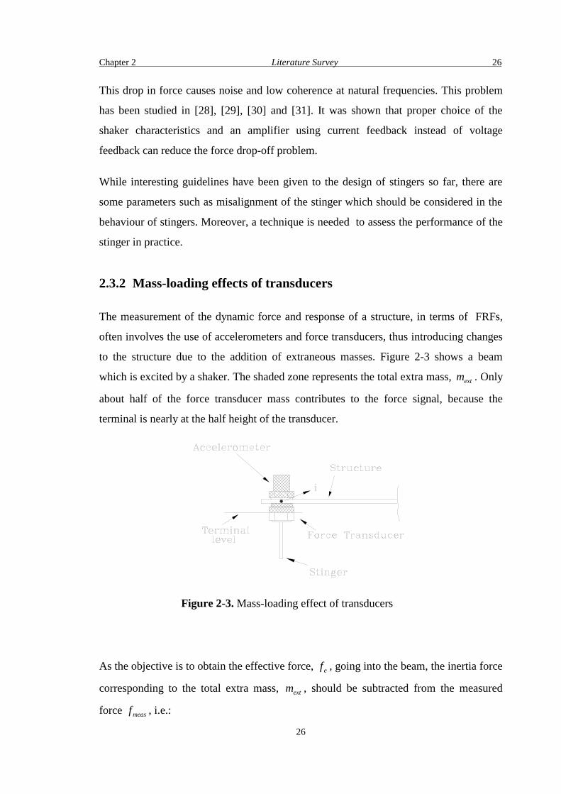
2.3.2 Mass-loading effects of transducers
The measurement of the dynamic force and response of a structure, in terms of FRFs,
often involves the use of accelerometers and force transducers, thus introducing changes
to the structure due to the addition of extraneous masses. Figure 2-3 shows a beam
which is excited by a shaker. The shaded zone represents the total extra mass, mext . Only
about half of the force transducer mass contributes to the force signal, because the
terminal is nearly at the half height of the transducer.
Figure 2-3. Mass-loading effect of transducers
As the objective is to obtain the effective force, f e , going into the beam, the inertia force
corresponding to the total extra mass, mext , should be subtracted from the measured
force fmeas , i.e.:

Chapter 2 Literature Survey 27
27
f f m xe meas ext i= − && (2-9)
From equation (2-9), the desired accelerance FRF can be obtained in the frequency
domain from:
AA
m Aii
iii
ext iii=
−
( )
( )1
(2-10)
This process is known as mass cancellation [5]. In general, some of the resonances will
always be somewhat affected by the masses of the transducers, so a mass cancellation
procedure is usually desirable, especially if the accelerometer position is to be changed
around the structure, as which is often the case. As shown above, the mass cancellation
procedure is quite straightforward for driving point FRFs. However, for transfer FRFs
the problem is much more difficult.
The effect of mass-loading was studied via the modal formulation of structural
dynamics, and in particular, by the modification theory formulated in modal space, as
explained by Synder [32] and further discussed by Avitabile & O’Callahan [33]. Based
on this study, Dossing [34] introduced the driving point residue method to predict shifts
of natural frequencies due to mass-loading effects. The equation of motion in modal
space for the mass modified structure is :
[ ] [ ][ ] [ ][ ]{ } [ ]{ }φ φ ωT
orM I x x∆ + + =&& 2 0 (2-11)
The eigensolution to equation (2-11) is :
[ ][ ][ ][ ] [ ]− + + =[ ] [ ]I MTr orφ φ λ ω∆ 2 2 0 (2-12)
Dossing simplified the problem further by solving for one mode at a time, assuming the
influence from other modes to be negligible. This assumption seems numerically
reasonable because the mode shape components are generally smaller than 1 and ∆Mi is

Chapter 2 Literature Survey 28
28
small too. Therefore the off-diagonal elements in the characteristic matrix are very small
compared to the ωor2 elements. The equation then reduces to :
{ } { }[ ]− + + =1 02 2φ φ λ ωr
T
r r orM[ ]∆ (2-13)
and if mass is added to only one DOF (point/coordinate) at a time, the problem reduces
to the scalar equation :
[ ]− + + =1 02 2φ φ λ ωir i ir r orm∆ (2-14)
Thus the relation between the natural frequency of the modified structure and the exact
natural frequency of the structure in terms of the added mass and the mode shape
component is :
ωω
φ
φ
r
or
ir
iriM
2
2
2
2
1
1=
+ ∆(2-15)
1 2φir represents the mass in this model which can be defined as “Apparent Dynamic
Mass” in DOF i associated with mode r. Using this method, it can be determined how
much the natural frequencies will change due to a mass-loading in a point. Or it can be
determined what the natural frequencies were before the accelerometer was attached to
the structure and modified its dynamics.
Decker and Witfeld [35] used the FRF substructuring technique, Structural Modification
Using experimental frequency Response Function (SMURF) to correct mass-loading
effects of transducers. The method of SMURF avoids the difficult and time-consuming
development of a modal model. For a structure modified by mass, m, the accelerance
FRF can be computed as :

Chapter 2 Literature Survey 29
29
A AA A
mA
lk lkj lk
jll
j
llj
( ) ( )( ) ( )
( )
( )( ) ( )
( )
ω ωω ω
ω= −
+1
(2-16)
in which m is negative. This equation has to be applied to every frequency value. In
equation (2-16) if Allj( ) is known the correct FRF can be computed. However,
measuring the driving-point FRFs at all measurement points is a very time-consuming
process and sometimes impossible. The authors suggested two techniques to
approximate All . In spite of some pitfalls the methods improve the measured FRFs.
However, noise was the main problem in the computations. To eliminate the effect of
noise in the computation, a weighted FRF method was introduced. The method is
successful in elimination of the effect of noise but causes discontinuity in the corrected
FRFs.
Silva, Maia and Ribeiro, [36] used coupling/uncoupling techniques to correct the mass-
loading effects of transducers for transfer FRFs which seems the most effective method
suggested so far. They showed that by coupling the structure with a lumped mass and by
mean of a series of relatively straightforward calculations the measured FRFs can be
corrected. The structure shown in Figure 2-4 is coupled with the mass m1 at point 1.
Using FRF coupling of substructures, the equation governing the new system is :
{ }A A
A A
A A A
mA m A A22
121
1
121
111
22 21 21
111 1
112 110 0 1
1( ) ( )
( ) ( )( )
=
+
−
+ −(2-17)
from which we have :
AA
m A111 11
1 111( ) =
+(2-18)
and
AA
m A121 12
1 111( ) =
+(2-19)
and

Chapter 2 Literature Survey 30
30
A Am A
m A221
221 12
2
1 111( ) = −
+(2-20)
Using equations (2-18), (2-19) and (2-20), three FRFs A11 , A12 and A22 , can be
obtained. Only three measurements are needed :
1 - Attach the accelerometer at point 1 and measure driving point FRF, A111( ) ;
2- Add another accelerometer at point 2 and measure transfer FRF, A121 2( , ) ;
3- At the same condition measure again driving point FRF, A111 2( , ) .
Figure 2-4. Modification of a structure by a mass
The interesting point is that it is possible to obtain the driving point FRF at point 2, A22 ,
without having to measure it. However, measurement problems of this method such as
the effect of noise on the computations were not studied by the authors. The same
technique was used by the authors for the evaluation of the complete FRF matrix, based
on measurements taken along a single column of the FRF matrix using different
accelerometers and dummy masses [37]. The technique inherently cancels the effects of
the extra masses of the transducers. This result is especially important to deal with
residual terms: It should be noted that there has not been found (so far) a way of relating
the residual terms of the measured curves to the residual terms of the unmeasured ones.
There is still no general applicable procedure to deal with the mass-loading effects of
transducers at non-driving points. Moreover, a method is needed to assess the quality of
the measurement due to the mass-loading effects of transducers.

Chapter 2 Literature Survey 31
31
2.3.3 Suspension effects on test structures
In modal testing, test structures are often suspended using soft springs to approximate a
free-free state of the structure. Free-free modal tests are popular because it is felt that the
effect of soft springs on the test structure is negligible. In free-free state of the structure,
the six rigid body modes no longer have zero natural frequencies, but they have values
which are significantly lower than that of the first elastic mode of the structure.
However, for flexible structures, the lowest elastic mode may interfere with the rigid
body modes. Therefore the support system is needed to be designed to avoid interference
of the rigid body modes on the lowest elastic mode of the test structure.
On the other hand, even soft springs introduce stiffness and damping into the system.
This added stiffness and damping of the suspension may significantly alter the modal
parameters of the elastic modes of the test structure.
Historically, there has been concern for suspension stiffness and its effect on measured
modal parameters of the test structure. Bisplinghoff, Ashley and Halfman [38] discussed
the effects of support stiffness and mass on the modal frequencies, based on the results
of Rayleigh [39]. Wolf [40] discussed the effects of support stiffness with regard to
modal testing of a car. Initially, he analytically studied the effects of a spring to ground
on a simple 2 DOF system. He then analysed data from a modal test of a car. He
concluded that to minimise the influence of the suspension system, the support system
should be attached to the most massive portion of the test system. He also reported that
the rule of thumb to simulate free-free boundary conditions is to design the support
system so that the rigid body modes are no more than one-tenth of the frequency of the
lowest elastic mode. But, for the case of vehicle tests, it is seldom possible to achieve
such a separation. He stated that test engineers frequently use 1:3 to 1:5 separation ratios
between rigid body modes and lowest elastic mode. He showed that such stiff supports
can lead to significant errors in the measured modal parameters.
Carne and Dohrmann [41] studied the effects of the support stiffness and damping on
measured modal frequencies and damping ratios. They developed the model used by
Wolf by including damping in the supporting system of the model. It was shown that for

Chapter 2 Literature Survey 32
32
a ligthly-damped structure even when the rigid body modes are no more than one-tenth
of the frequency of the lowest elastic mode, the measured damping can be far from the
true damping.
Lindholm and West [42] investigated the effects of suspension stiffness on a beam using
different shock cord lengths and thickness. A perturbation study was done to determine
what effects suspension stiffness would have on the mode shapes of the beam. In order
to update the analytical model of the beam, optimisation routines were used to achieve a
minimal difference between the analytical mode shapes and the experimental mode
shapes. This study is especially important because the updating routine was done using
several experimental mode shapes at once to find the optimum one.
It can be concluded that although suspension springs may have serious effects on the
measurement, there is still no method to correct the effects of the suspension springs on
the measured FRFs. Moreover, a method is needed to assess the quality of the
measurement due to the effects of the suspension springs on the measurement.
2.4 Perturbation of Boundary Condition (PBC)
In a standard modal testing method, a modal model is normally based upon a single
testing configuration (i.e.: free-free, fixed boundary condition, etc). The number of
modes which can be extracted by this method consists typically of 10 to 40 lowest
frequency modes for the given test configuration. This data base is far too small to
completely update an FE model, and , in general, is still too small to develop an accurate
modal model for dynamic modification. As a result, a new testing procedure has been
developed which is referred to as the Perturbed Boundary Condition (PBC) testing
method. In the PBC method, the system is tested in a number of different configurations;
each configuration consists of the system with one or more of its boundary conditions
perturbed. The different boundary conditions change the original modal space of the
system. (Figure 2-5).

Chapter 2 Literature Survey 33
33
Figure 2-5. Perturbation of boundary condition (PBC)
Basically, two boundary condition perturbations are being examined. The first is a
stiffness change; the second is a mass addition at the boundary point. The mass addition
technique is specially targeted at stiffer structures while stiffness modification testing is
targeted towards low frequency flexible structures tested in a free-free configuration
where the test support system interferes with the accuracy of the resulting modal model.
The use of PBC allows for :
1. Estimination of rotational degrees-of-freedom.
2. Elimination of support effects.
3. Simple boundary simulation
4. Mode enhancement
Simley and Brinkman [43] employed the mass additive testing approach to show the
importance of rotational degrees of freedom and to estimate them. For a simple beam the
rotational mode shape was computed from a set of translational data. However, it was
not possible to achieve the necessary resolution in the areas where it is needed.
One of the first PBC methods applied to Finite Element modelling verification was
applied to large flexible structures by constraining to ground the interior points of the
structure and verifying the constrained structure against an FEM model [44], [45], [46],
[47].These large flexible structures were difficult to test free-free because the
Chapter 2 Literature Survey 34
34
frequencies of the elastic modes were too close to the rigid body modes of the structure.
Constraining the structure eliminated the support problem.
Coleman and Anderson [48] used mass additive testing for a simple boundary simulation
to approximate an in-situ configuration for a space shuttle flight pay-load. Traditionally a
fixed-base modal test has been performed as a means of verifying the coupled-load
mathematical model. An alternative method, a free-free configured payload using mass
loaded boundary conditions , was presented as a means of verifying the coupled loads
model. The method is cost-effective in that an expensive test fixture with unknown
boundary conditions is replaced by a relatively inexpensive, reusable suspension system
that produces a known boundary condition which does not contaminate the modal test
results with fixture-coupled modes or boundary condition uncertainties.
Mode enhancement utilises certain modifications to a structure to allow for the
measurement of a mode which is normally outside the measurement bandwidth, thereby
allowing verification of potentially important system modes. Mode enhancement has
been examined as a method for incremental updating an FE model using the various
system models for each configurations. Gwinn, Lauffer and Miller [49] used a technique
for synthesis of mathematical models of structural systems using experimentally-
measured component modes that have been enhanced by mass interface loading. With
this technique, individual components were tested with arbitrary discrete masses added
to interface points. The effect of the interface mass was then analytically removed before
the component was assembled into the global system. Results from this study indicated
significant improvement in the assembled system property.
Recently, procedures for utilising a PBC database for updating of finite element models
were being developed [50], [51]. These techniques are currently at an early stage of
development.
Brown, Pierre and Barney [52] introduced a procedure for estimating the free-free modal
characteristics of a system by testing multiple constrained states. The procedure utilises
PBC to decouple the effective forces from the true excitation forces and reduces the
influences of the constraints on the modal parameters. A frequency domain Auto
Regressive Moving Average (ARMA) model was used to calculate the system’s free-free

Chapter 2 Literature Survey 35
35
characteristics and to provide additional system model information for Finite Element
(FE) correlation.
Structural modifications in the form of mass and stiffness additions are usually applied
to the basic equation for describing the dynamics of a lumped parameter system as small
additions to the respective free-free mass and stiffness matrices.
[ ] [ ] [ ] { } { }( )M M s C s K K X F+ + + + =∆ ∆2 (2-21)
Equation (2-21) can be rearranged to allow for a direct solution of the free-free system
characteristics :
[ ] [ ] [ ] { } { }( ) { [ ] [ ]){ }M s C s K X F M s K X2 2+ + = + − −∆ ∆
{ } { }= + =F F Fe total{ }
(2-22)
where { }Fe is the matrix of the effective forces. It can be seen that by measuring the
displacements of the system, as well as input forces, all of the terms on the right hand
side of the equation (2-22) are known (given that the modification matrices are known)
and the free-free system parameters are obtainable.
By using the ARMA model the effective forces, the unmodified system’s characteristics
may be obtained without the need for an FRF calculation. The equation for describing
the dynamics of a lumped parameter system is shown as :
[ ] [ ] [ ] { } { }( )M s C s K X Ftotal2 + + = (2-23)
or :
([ ] [ ]) { } ([ ] [ ]){ } [ ] { } [ ] { }M C s X M K X M F I s Xtotal− − −+ − = −1 1 1 2 (2-24)
or :
[ ] { } [ ]{ } [ ]{ } [ ] { }A s X A X B F I s Xtotal1 0 02+ + = − (2-25)

Chapter 2 Literature Survey 36
36
The above equation is a standard Auto-Regressive Moving-Average (ARMA) model. Or
in matrix form:
[ ][ ]A A B
sX
X
F
I s X1 02
= − (2-26)
To solve the above equation there must be at least as many measured vectors as active
modes. These measured vectors can consist of the various test configurations at several
frequencies. By condensation of different configurations, the resulting matrix of equation
(2-26) takes on the form of :
{ } { }{ } { } { }{ } { } { }
{ } { } { }[ ]...
...
...
..}{.
][
2221
211
21
211
211
221111
01
PQP
PQP
PQP
PQP
XXX
FFF
XXX
XjXjXj
BAA
ωωω
ωωω
−−−
=
(2-27)
in which P and Q refer to different configurations. The ARMA coefficients , the
[ ]A si and [ ]B si , can be solved by using the pseudo-inverse of the measurement matrix
in equation (2-27).The averaging property of this procedure uncorrelate the effective
forces and allow for a solution.
Equation (2-23) can be arranged in the form of :
[ ] [ ] [ ] { } { }( ) ( ) [ ]A s A s A X s B Ftotal22
1 0 0+ + = (2-28)
Equation (2-28) is the Laplace domain UMPA model for PBC test data. The same
procedure which was explained for the ARMA model is applied here to find the
unknown UMPA coefficient matrices, [ ]Ai and [ ]Bi in equation (2-28).

Chapter 2 Literature Survey 37
37
Brown, Vold and Shumin Li [53] used the scaled least square method with an UMPA
model to find the free-free parameters. They showed that the unknown coefficient can be
estimated from solving the following equation :
{ } { }{ } { } { }
{ } { } { }{ } { } { }[ ]..(.)()(
...
...
..}{)(.)()(
]~~~
[
221111
211
221111
22
212
112
1
01
ωωω
ωωωωωω
PQP
PQP
PQP
PQP
XXX
FFF
XjXjXj
XjXjXj
BAA =
(2-29)
in which P and Q refer to different configurations. Since both X ( )ω and F( )ω
normally contain measurement errors, a more accurate estimate of the UMPA
coefficients can be obtained by using the total least-square method. This method allows
for the cancellation of the effect of noise and provides unbiased estimates of the modal
parameters. The procedure is reported in [53].
It seems that the PBC method can provide an effective tool to deal with measurement
problems such as mechanical errors which are not possible using conventional modal
testing. However, so far the PBC concept has been applied only for spatial models (mass
and stiffness models) and not for response models (FRFs) which is the subject of this
thesis.
2.5 Measurement of rotational DOFs
Rotational DOFs are present, in most cases, in 75% of the complete FRF matrix.
Knowledge of them can therefore be of extreme importance to obtain reliable results
when doing calculations related to coupling, structural modification, Finite Element
model updating, joint identification, etc. However, there are neither reliable angular
transducers available, nor a practical means of applying moment excitations.
For this reason most of modal analysis techniques tend to be developed by avoiding as
much as possible the measurement of rotational FRFs, or by minimising the effects of
not knowing them. Condensation and expansion techniques, mainly when addressing FE
updating methods, are sometimes used to circumvent the problem.

Chapter 2 Literature Survey 38
38
Kistler’s 8832 TAP system simultaneously measures one translational and one rotational
acceleration. The system uses the dynamic deformation of piezoelectric cantilever beams
as the transduction principle [54]. However, this system could not adequately solve the
problem of measurement of the rotation. Aside from rotational accelerometers, several
other methods have been used for rotational measurements and obtaining rotational
FRFs which are discussed below.
2.5.1 The exciting block technique
This technique is based on the measurement of accelerometers properly placed on an
additional block which is attached to the point of interest on the structure. The theory of
exciting block is fully developed in references [55] and [56]. An engineering application
of this technique is presented in [57]. However, the cross-sensitivity of accelerometers
and additional mass and local stiffening of the block could cause problem in this
technique. These are explained in references [58] and [59]. It was shown in [60] that it is
possible to estimate accurate rotational response/force FRFs but the more difficult FRFs
to estimate are those related to moment excitations.
2.5.2 The finite difference technique
This technique is based on the estimation of the rotational properties from spatial
derivatives of translational data which in turn are gathered by accelerometers placed on
the structure at convenient distances from each other [61] , [62]. This approach presents
an advantage over the exciting block technique since the mass and stiffness properties of
the structure are not altered so much in the measurement region. The distance between
measurement points is critical for the correct estimation of rotational FRFs [59] .
The derivation of the translational data can be accomplished using either first-order [61]
or second-order [62] finite difference formulas. The derivative approaches, however ,
proved to be effective only for simple structures [63] ,[64]. The fitting function is an
alternate approach to cover either simple or complicated structures. The fitting function
approach is divided into two groups : polynomials [65], [66] and splines [64], [67], [68]
fitted to translational data. These techniques have shown considerable potential. The

Chapter 2 Literature Survey 39
39
polynomials are ideal for representing uncomplicated relationships. The main
disadvantage, however, is the inability of polynomial fits to produce acceptable results
for the higher frequency modes. Splines, on the other hand, are more suitable for
representing very complex surfaces. On the other hand, splines are computationally
efficient and more stable numerically than polynomials.
2.5.3 Laser interferometry
Laser interferometry is a technique in which by analysing the difference in phase
between a measurement beam, reflected off the object of interest, and a reference beam,
displacement can be detected with a resolution on the order of nanometers. Coupling two
or more measurement beams, offset laterally by a fixed distance, allows rotation about
one axis to be measured. While offering a very accurate means for sensing simultaneous
rotations and translations, laser interferometry requires expensive, unwieldy analysis
equipment.
Several application-specific devices capable of multi-axis measurement systems have
been reported. Automotive researchers have developed a laser-based system for piston
measurement [69]. In this system a collimated light beam is aimed through an optical
port machined into the cylinder head at the piston surface and receives the reflected
beam on to two position sensing photodetectors. The detector outputs are then used to
determine the axial position and tilt angle of the piston. However, the hardware limits on
resolution and the position and rotational angle of the piston were not effectively
established.
Another system developed for positioning of a magnetically levitated micro-manipulator
relies on three light sources and three photodetectors [70]. Opaque wings with a single
pinhole in each are attached symmetrically to the manipulator. The wings are positioned
so that a light source and a detector are on opposite sides of each pinhole. As the wings
move, the light spots sensed by the detectors move, and the corresponding output
information can be processed to determine the manipulator’s new position. Since the
wings are all coplanar, this system is only capable of measuring four degrees of freedom,
two translational and two rotational.

Chapter 2 Literature Survey 40
40
Sommer, Trthewey, Caefo and Rieker [71] used Laser interferometry for a noncontacting
measurement approach, capable of simultaneously sensing one dynamic translation and
two dynamic angular rotations. The transducer system is based on the positional
measurement of two laser beams reflected from a planar target. Using the geometric
orientation between the incident light beams and the corresponding reflections onto two
position sensing photodetector, the translation, pitch angle and roll angle of a planar
target can be determined. The reported resolution is 40 µm for translation and 0.02
degrees for rotation with a working range of 2 3× mm and ± 5 0. degrees. Bokelberg,
Sommer, Trethewey and Chu [72] developed the technique for simultaneous
measurement of three translational and three rotational displacements of a vibrating
object. The system is based on sensing the positions of three collimated light beams
reflected from a tetrahedral target attached to the vibrating object. The dynamic position
of the target is determined by using the system geometry , coordinate transformations
and kinematics closure procedure.
This method offers accurate results but it is vulnerable to noise in the computations and
the mass and stiffness properties of the structure altered by the attachment of tetrahedral
target.
2.5.4 Laser-based 3D structural dynamics modelling
Modelling the laser-based experimental 3-D (3 dimensional) structural dynamics
response of structures under test is one aspect of a larger body of research defined as
structural imaging. Structural imaging includes shape and dynamic response modelling
from laser measurements, and it then culminates with the visual display and analysis of
the complete shape and dynamic response models. This method consists of taking three
single-dimension measurements from different vantage points and then transforming
them into an orthogonal triad of velocities. The measurements do not need to be in an
orthogonal orientation. This method has evolved from the work of R. M. Huffaker [73].
Huffaker used a Laser Doppler system to measure the three-dimensional velocity of a
gas. To measure the velocity he had one laser shooting into the gas and three laser

Chapter 2 Literature Survey 41
41
detectors measuring the velocities. The velocities were then transformed into an
orthogonal coordinate system. His method would not work for the measurement of the
dynamic behaviour of a structure because it depends upon the transparency of the gas.
Most structures are opaque, thus blocking the laser light. However, Huffaker’s method
was modified by Donavan [74] for use on structures. Donavan used a Laser Doppler
velocimeter that had the laser and detector all in the same unit. The unit actually
measures velocity in the same direction as the laser beam and makes measuring dynamic
response of a structure possible. Donavan’s approach used one laser that took all three
velocity measurements in three different positions. The laser had to be physically moved
to each defined location separately. In many measurement situations it is difficult to
position the laser accurately.
Mitchell and Abel [75] used a computer algorithm called the Four Point Registration
Method to accomplish the locating of the laser in space. The method requires that the
structure have four points marked with their exact coordinates known, in the reference
coordinate system. These four points are called registration points. At each new laser
position the laser beam needs to be moved, or scanned, to the first registration point.
This is done by electronically moving the two internal scanning mirrors.
Mitchell and Galaitisis [76] developed a theoretical technique to extract drilling-angular
velocities (θz ) from translational velocities using high spatial density data from a
scanning Laser Doppler Vibrometer (LDV). where z is the out of plane direction.
Kochersberger [77] and Sun [78] developed a method for angular velocity of in-plane
velocities using a DFT-IDF technique (Discrete Fourier Transform-Inverse Discrete
Fourier Transform). Their effort resulted on measurement of two more DOFs; rotation
about x and y axes where x and y are in-plane directions (θ x and θ y ).
Lindholm [79] used a registration procedure in which the laser is “manually” aimed at
several points of known location on the structure. Three translation coordinates and three
rotation angles are then estimated using a weighted non-linear least-squares procedure in
which differences between predicted scanning angles and measured scanning angles
(used to hit the registration points) are minimised.

Chapter 2 Literature Survey 42
42
Although laser-based 3D techniques are expensive and time-consuming processes, they
do give a general and continuous data about the dynamic behaviour of the most of the
points of the structure. However, this is not an easy task using other methods of
measurement.
2.5.5 Scanning Laser Doppler Vibrometer (LDV)
An LDV beam can be scanned continuously along a line on a vibrating surface giving a
modulated output which can be used in a number of ways to analyse structural vibration.
Stanbridge and Ewins [80], [81], [82] used a continuously-scanning LDV to measure
rotational response of the structure. They found that the response signal contains three
components : one at the excitation frequency, giving the translational response, the
others with an equal distance from the excitation frequency, giving the rotational
responses. Two linear sine scans along orthogonal in-plane axes are sufficient to find the
in-plane rotational vibration. However, by using a circular scan it is possible to obtain
this information with just one measurement.
Stanbridge and Ewins [83] developed a new conical-scanning technique which gives an
easily-quantifiable measure of the magnitude and direction of the vibration of a point,
even if the vibration is in-plane. It has been shown that the total state of translational
vibration and rotational vibration except drilling angular velocity can be derived using a
short-focus lens to produce a conical scan. This method, however, is in its early stage
and needs to be developed for practical cases.
2.6 Noise
Measured FRFs contain a certain amount of noise, a feature inherently present in all
measured data. The success of the methods based on modal testing depends on the
quality of data and, especially on the level of the experimental noise. Estimators are used
to deal with the problem of noise. Bendat and Piersol defined H1 [84] estimator as:
HG
G
G
G Gxy
xx
uv
uu mm1 = =
+(2-30)

Chapter 2 Literature Survey 43
43
where Gxy is the cross spectrum between the measured force signal and the measured
response signal, Guv is the cross spectrum between the true force signal and the true
response signal, Gxx is the auto spectrum of the measured force signal, and Gmm is the
auto spectrum of the noise from the force transduction system. The H1 estimator
underestimates the magnitude of the FRF near resonance. At resonance the structure
looks like a short circuit (low impedance) to the shaker. This results in large losses
within the power amplifier-shaker itself and a low-force input. The low-force input
reduces the level of signal-to-noise ratio and allows the force transducer output signal to
approach the transducer noise. In this case, the result is biased. However, the bias is
caused only by the noise from the force transduction system. Transducer noise has no
influence on such bias provided the estimates are sufficiently averaged.
This is the worst place to have erroneous estimates of an FRF. The reduction of the
magnitude in this resonance area can effectively influence the estimation of the modal
parameters. The first alternate estimator H2 [85] was proposed in the early 80’s. This
estimator was designed to yield an upper bound estimator on the FRF. The H2
estimator is defined as :
HG
G
G G
Gyy
yx
vv nn
uv2 = =
+ (2-31)
where Gyy is the auto spectrum of the measured response signal, Gvv is the auto
spectrum of the true response signal, and Gnn is the auto spectrum of the output
transducer noise. The H2 estimator is a good estimator of the FRF at resonance even in
the presence of the noise from the force transduction system. At resonance the response
signal is very large with respect to the system noise. Thus, the numerator approaches the
true auto spectrum of the response. The denominator of equation (2-31) approaches the
true cross spectrum with appropriate averages. The problem with this estimator is that it
has a poor quality at the anti-resonances within the FRF.

Chapter 2 Literature Survey 44
44
After estimator H2 , a series of other FRF estimators were proposed [86], [87], [88]. The
Hs [86] and the Hv [89] estimator were the closest to an optimal estimator over the full
range of the FRF. However, these estimators required another estimator for the various
levels of uncorrelated content entering the estimation process.
In 1985 Goyder [90] presented an idea for the improvement of the FRF estimation
process. He suggested :
$HG
G
G
Gc ys
xs
vs
us
= = ( 2-32)
where Gys is the cross spectrum between the excitation source signal and the measured
response signal, Gvs is the cross spectrum between the source signal and the true
noiseless response signal, and similar definition between the measured force signal and
the excitation source signal. The details of this methodology (Equation (2-32)) were
delineated by Cobb [91], [92]. He explained the unbiased estimator properties of the
$H c estimator and defined the finite sample size bias error effect. Moreover, he defined a
technique for estimating the confidence bounds on the FRF for the first time and
proposed a method for the determination of the source of and the quantity of noise
associated with each transducer and shaker in the system. This new FRF estimator
provides one of the best methods for the unbiased estimation of the FRF.
2.7 Conclusions
• Modal testing techniques can be very sensitive to even small changes in the
structure’s dynamic behaviour, such as those that are usually considered negligible in
the measurement. So there is a need to investigate the effect of the small changes in
the system relating to the mechanical devices such as accelerometers, suspension
springs and stingers.
• On a more philosophical note, the expectations from a high quality modal test are not
formulated very clearly. The maximum allowable changes in the measured FRFs due

Chapter 2 Literature Survey 45
45
to the effects of the measurement errors and their relation to measurement accuracy
need to be defined further.
• There is still no general applicable procedure to deal with the mass-loading effects of
transducers at non-driving points. Moreover, a method is needed to assess the quality
of the measurement due to the mass-loading effects of transducers.
• Suspension springs may have serious effects on the measurement but there is still no
method to correct the effects of the suspension springs on measured FRFs. Moreover,
a method is needed to assess the quality of the measurement due to the effects of the
suspension springs on the measurement.
• While some researchers have given interesting guidelines to the design of stingers,
there are some parameters such as misalignment of the stinger which should be
considered in the behaviour of stingers. Moreover, a technique is needed to assess
the performance of the stinger in practice.
• The PBC method seems quite promising for the assessment of the quality of the
modal testing in the sense that different configurations for an identical test structure
allow for the detection of the measurement errors and obtain the exact FRFs.
• In spite of extensive research for the measurement of rotational DOFs, no generally
applicable procedure has been found so far. The more difficult FRFs to obtain are
those related to moment excitations.
• Noise is the main problem in the computations of the methods based on the modal
testing results.

Chapter 3 Correction of mass loading effects of transducers in modal testing46
46
CHAPTER 3
Correction of mass-loading effects
of transducers in modal testing
3.1 Introduction
The mass-loading effect of transducers is one of the sources of error in modal testing.
A transducer mounted on a vibrating system changes the dynamics of the structure
and introduces errors into measured FRFs. One problem with this is the production of
unrealistic results, which cause the measured resonant frequencies to be less than the
correct values. A further problem is the inconsistency of the data base when using a
series of measurements with roving transducers in order to acquire data for modal
analysis. Data inconsistency can cause severe problems in the curve-fitting process,
particularly when applying a modern global parameter estimation algorithm.
It is desirable to cancel the effect of the extra masses on a measured FRF. The mass
cancellation technique for transducers at the driving points has been explained by
Ewins [5]. However, there are few publications about quantification of the mass-
loading effects, caused by a measuring transducer, at the non-driving points [34],
[94].
The method of Structural Modifications Using experimental frequency Response
Functions (SMURF) was investigated first to avoid the difficulties of developing a
modal model for structural modification proposes. This method was introduced by
Klosterman [95].
In this chapter, the SMURF method is used to revisit the problem of mass-
loading effect of transducers. Based on this analysis, a general solution for
correction of the mass-loading effects of transducers is proposed.

Chapter 3 Correction of mass loading effects of transducers in modal testing47
47
This work was done prior to and independently of the work published in [36] and then revised
and published in IMAC 1998 [93].
3.2 Theory
3.2.1 Mass modification
Changes in the FRF of a system due to mounting a mass can be estimated using direct
substructuring technique SMURF as follows :
Figure 3-1(a) indicates a structure which has been rigidly connected to the second
system of a mass. The connection is at point j and in x direction. The force excites the
structure at point i and the response is measured at point l. Figure 3-1(b) indicates the
free body diagram of the system.
Figure 3-1. Mass modification
As is usually the case in modal testing, the system is presumed to be linear. The
equations governing the coupled system are:
X F Rl li i lj j= +α α (3-1)
X F Rj ji i jj j= +α α (3-2)

Chapter 3 Correction of mass loading effects of transducers in modal testing48
48
X Rm mm m= α (3-3)
where :
α ωmm m= −
12
(3-4)
and the constraining equations are :
X Xj m= (3-5)
R Rj m+ = 0 (3-6)
Elimination of the reaction forces and displacements at the connection point results
in :
X F Fl li
ji lj
mm jji li
ji= −
+=( ) .( )α
α αα α
α(3-7)
in which αlij( ) is the modified receptance function between points l and i when the
second system is a mass with the amount of m and connected rigidly to the original
system at point j. From equation (3-7) one can immediately relate αlij( ) and the
original receptances, thus :
α αα α
α αlij
li
ji lj
mm jj
( ) = −+
(3-8)
in which α α α αli ji lj jj, , , are the original receptances, namely for the system without
the accelerometer. Multiplying both sides by − ω 2 , the relation between accelerances
is :
A AA A
A Alij
li
ji lj
mm jj
( ) = −+
(3-9)
Equations (3-8) and (3-9) are general equations for modifying a system by the
connection of a mass, m.

Chapter 3 Correction of mass loading effects of transducers in modal testing49
49
One can develop three special cases which are applicable in the mass cancellation
technique suggested in this work.
(a) For the special case of an attached accelerometer, the point of response
measurement is the same as the point of connection (j=l , l ≠ i) (Figure 3-2) .
Equation (3-9) can then be rewritten as :
A AA A
A Alil
lili ll
mm ll
( ) = −+
(3-10)
where Amm is :
Ammm =1 (3-11)
Figure 3-2. Mass modification of an accelerometer
Inserting equation (3-11), equation (3-10) can be simplified as :
AA
mAlil li
ll
( ) =+1
(3-12)
Equation (3-12) shows how the measured FRF Alil( ) is related to the correct
accelerances, Ali and All .
(b) For the driving point accelerance (j=l=i), equation (3-12) can be summarised as:
AA
mAlll ll
ll
( ) =+1
(3-13)

Chapter 3 Correction of mass loading effects of transducers in modal testing50
50
which is nothing other than the standard mass modification at the driving point.
(c) For the case that there are two accelerometers attached at points i and j (i=l)
(Figure 3-3(a)), one can consider mass mj is attached at point j to the system
consisting of mass mi and the structure B (Figure 3-3(b)).
Figure 3-3. Uncoupling of one mass
In this case equation (3-9) can be summarised as :
A AA
mA
iii j
iii ji
i
jjj
i
( , ) ( )
( )
( )
( )= −
+
2
1 (3-14)
Equations (3-12) , (3-13) and (3-14) can be derived using the FRF coupling technique
which is the same idea suggested by Maia, Silva and Riberio [36].
3.2.2 Correction of the mass-loading effects of transducers
Equation (3-12) shows how the measured accelerance Alil( ) is related to the correct
accelerances, Ali and All . In equation (3-12), If Alil( ) and All are known, Ali , the
correct transfer FRF, can be computed. Alil( ) is obtained by measurement. If All
l( )
could be measured, All would be obtainable using equation (3-13) . However,

Chapter 3 Correction of mass loading effects of transducers in modal testing51
51
measuring FRFs at all driving points is a time-consuming process. Furthermore in
most cases the excitation and response measurement at some points on the test
structure is impossible. To overcome the problem of obtaining All , one may consider
two measurements with two different accelerometers with different masses ( Figure 3-
4).
Here the magnitude of m1 is different to that of m2 . The equations governing the
systems are :
AA
m A
AA
m A
lil li
ll
lil li
ll
( )
( )
=+
=+
1
1
1
2
(3-15)
Figure 3-4. Measurement using two different accelerometers
in which Alil( ) is different from Ali
l( ) . In matrix form, equation (3-15) can be written
as :
1
1
1
1
1
2
Am
Am
A
Ali
l
lil
li
ll
( )
( )
−
−
=
(3-16)

Chapter 3 Correction of mass loading effects of transducers in modal testing52
52
Equation (3-16) is a combination of two linear equations and can be solved for Ali
and All :
A
AA
m
Am
li
ll
lil
lil
=−
−
−1
1
1
1
1
2
1
( )
( )
(3-17)
With this procedure one can obtain two correct FRFs ( Ali and All ) by undertaking
two different measurements ( Alil( ) and Ali
l( ) ). So the mass cancellation has been
accomplished for transfer FRFs. Moreover, the driving point FRF at point l has been
found without having to measure it. This method is basically the same as that
suggested in [36]. However, the present computational procedure is more systematic
and is especially helpful in dealing with noise, as discussed below.
3.3 Demonstration and verification of the method
3.3.1 Validation of the method
To prove the validity of the method presented in section 3.2.2, a 12 DOF system of
masses, springs and dampers has been considered in a simulated test (Figure 3-5).
Table 3-1 shows the specifications of the system.
Table 3-1 . Parameters of the 12 DOF system
DOF Mass (Kg) Stiffness (N/m) Damping (Ns/m)
1 3 7000 0.3
2 1.3 10000 0.2
3 1.5 5000 0.1
4 1 2000 0.8
5 1 10000 0.5
6 2.5 5000 1.6
7 1.5 10000 1
8 1 3000 0.3
9 1 5000 0.8

Chapter 3 Correction of mass loading effects of transducers in modal testing53
53
10 2.5 10000 0.3
11 1.2 4000 0.5
12 1 8000 0.9
Figure 3-5. A numerical example of 12 DOF system
The system is excited at point 2. An accelerometer has been attached to the system at
point 1 to measure transfer FRF, A12 , in the simulated test (Figure 3-5). In order to
show the difference in graphical representations clearly, the mass of the accelerometer
has been exaggerated ( ma = 1.5 Kg). Figure 3-6 shows the comparison of the
accelerances , A12 , of the system without accelerometer (solid line) and with
accelerometer (dashed line).
For correction of the measured FRF, another accelerometer with the mass of 1.2 Kg
was used at point 1 in the simulated measurement . Using equation (3-17) the correct
values of A11 and A12were calculated. Figure 3-7 shows the comparison of the true
FRF, A12 , and the measured FRF, A121( ) , after correction. As can be seen, the
measured FRF, A121( ) , coincides with the true FRF after correction.

Chapter 3 Correction of mass loading effects of transducers in modal testing54
54
Figure 3-6. Comparison of the accelerances, A12 , of the system without
accelerometer (solid line) and with accelerometer (dashed line)
Figure 3-7. Comparison of the accelerances, A12 , of the system without
accelerometer (solid line) and with accelerometer (dashed line) after correction
The same coincidence was obtained for A11 , (not shown here)

Chapter 3 Correction of mass loading effects of transducers in modal testing55
55
3.3.2 Practical considerations
The method suggested in this article is exact, but in practical situations may be
vulnerable to measurement errors such as noise. To understand the scale of the
problem, two further simulated tests were conducted. The specifications of these tests
are given in Table 3-2.
Table 3-2. The effect of accelerometer mass on the computations
FRF A12
The mass of the first accelerometer 0.1 (Kg)
The mass of the second accelerometer (1st example) 0.11 (Kg)
The mass of the second accelerometer (2nd example) 0.2 (Kg)
Percentage of noise 5%
Frequency Range 1-10 (Hz)
The FRFs of the system were polluted by adding random noise using the following
relation:
(A RAN Ali li= + × × − ×[ ( )]1 2 1α (3-18)
where (Ali is the noisy accelerance,α is the percentage of noise, RAN is a random
value between 0 and 1 and Ali is the accelerance without noise. The percentage of
noise in this example is 5%.
Two different masses were used for the second accelerometer. The mass of one of
them was close to the mass of the first accelerometer (0.11 Kg) while the mass of the
other one was quite different (0.2 Kg). Figure 3-8 shows the result of the correction
with the 0.11 Kg mass. Figure 3-9 shows the result of the correction with 0.2 Kg
mass. It is clear that this calculation is sensitive to noise when the two masses are
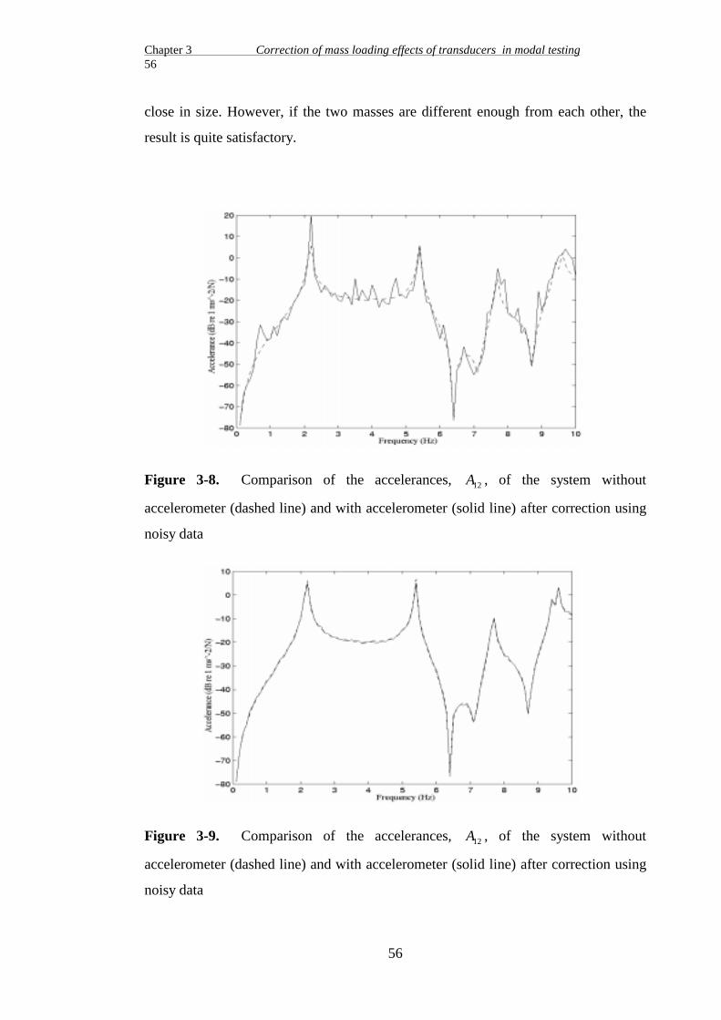
Chapter 3 Correction of mass loading effects of transducers in modal testing56
56
close in size. However, if the two masses are different enough from each other, the
result is quite satisfactory.
Figure 3-8. Comparison of the accelerances, A12 , of the system without
accelerometer (dashed line) and with accelerometer (solid line) after correction using
noisy data
Figure 3-9. Comparison of the accelerances, A12 , of the system without
accelerometer (dashed line) and with accelerometer (solid line) after correction using
noisy data

Chapter 3 Correction of mass loading effects of transducers in modal testing57
57
The reason for this can be found by looking carefully at equation (3-17). The matrix :
1
1
1
2
Am
Am
lil
lil
( )
( )
−
−
(3-19)
will be ill-conditioned if two rows of the matrix are highly correlated. As m1 becomes
closer to m2 , Alil( ) becomes closer to Ali
l( ). Consequently, two rows become more
dependent on each other and in the presence of noise, the inverse of the matrix is
unrealistic. Therefore, it is important to choose suitable masses to avoid unrealistic
results.
3.3.3 Experimental case study
A simple beam was used for the experimental validation of the method presented in
this chapter. The beam was made of mild steel, and had dimensions 20 0 6 44× ×. cm
and a weight of 0.412 Kg. Figure 3-10 shows the set-up of the equipment for a
hammer test of the beam. Although 6 directions must be considered, the motion of the
beam was considered in only two directions: one axial direction (z) and one rotational
direction (θ y ). The experimental model of beam was divided in to 6 equal elements
and was tested in a free-free configuration, suspended by soft elastic cords attached to
the beam at points 2 and 6 (see Figure 3-10).The excitation was applied at its neutral
axis at point 5 and the response was measured at point 4 using a light accelerometer
with a mass of 0.004 Kg. To conduct a genuine test, it was assumed that the structure
consisted of the beam and the accelerometer. Then, two different extra masses are
added to the accelerometer on two different tests and the beam was measured. These
extra masses were assumed to be two different accelerometers with different masses.
There are two benefits in this assumption. First, an exact result (without any extra
mass) of the structure can be obtained. Second, one accelerometer is used for all of
the measurements. Therefore, this procedure allows us to eliminate all the other
possible sources of the error (except for mass-loading effect) in the measurements.

Chapter 3 Correction of mass loading effects of transducers in modal testing58
58
The extra mass for the first test was 0.029 Kg (7% of the mass of the structure) and
for the second test was 0.048 Kg (11.5% of the mass of the structure). The structure
was tested once without extra masses installed to obtain exact transfer and point FRFs
for comparison purposes. Figure 3-11 shows the comparison of the exact receptance
function (α 45 ) and the measured receptance function around one of the resonances of
the beam using two extra masses to represent the accelerometers. In this case the
measured recptance was affected by the extra masses and the resonance was shifted to
the left. Using the method suggested in this chapter for the correction of the mass-
loading effects of transducers, the FRFs were corrected. Figures 3-12 and 3-13 show
the comparison of the computed FRFs and the exact FRFs for the transfer and point
FRFs, respectively. An interesting point is that the driving point FRF(α44 ) was
obtained without measurement. Figure 3-13 shows that the corrected FRF and the
exact FRF match around resonance while at other points the computed FRF is more
noisy. Fortunately, most of the information from modal testing is from the resonance
areas.
Figure 3-10. Experimental set-up for hammer testing of the beam

Chapter 3 Correction of mass loading effects of transducers in modal testing59
59
Figure 3-11. Measurement of the structure affected by extra masses (α 45 )
Figure 3-12. The comparison of the computed transfer FRF and the excat FRF (α 45 )

Chapter 3 Correction of mass loading effects of transducers in modal testing60
60
Figure 3-13. The comparison of the computed point FRF and the exact FRF (α44 )
3.4 Calibration of the test set-up using the correction method
One of the interesting applications of the method suggested in section 3.2.2 is
checking the calibration of the test set up. As with all measurement process, it is
necessary to calibrate the equipment which is used in modal testing during each test.
It is customary to use a simple rigid mass-like structure to calibrate the equipment. If
the accelerance of this rigid mass is measured, then the FRF obtained should be equal
to (1/mass) over the entire frequency range, and this is a quantity which can be
accurately determined by weighing.
In this section an alternative method is presented to calibrate the test set up by
modifying the test structure. It was shown that the measured FRFs can be corrected if
the measurement is repeated with an accelerometer of different mass. The answers to
equation (3-17) can be simplified as :
Am m
m
A
m
A
li
lil
lil
=− +
−+
2 1
2 1( ) ( )
( 3-20)
and

Chapter 3 Correction of mass loading effects of transducers in modal testing61
61
AA Am
A
m
A
lllil
lil
lil
lil
=− +
−+
1 1
2 1
( ) ( )
( ) ( )
(3-21)
Now suppose that the test set up is uncalibrated. Then the measured FRFs shift
upwards or downwards by a factor like α with respect to the calibrated FRF.
Therefore, the measured uncalibrated FRFs are equal to calibrated FRFs multiplied by
α . For uncalibrated FRFs, equations ( 3-20) and (3-21) are changed as:
~
( ) ( )
Am m
m
A
m
A
Ali
lil
lil
li=− +
−+
=2 1
2 1
α α
α (3-22)
and :
~( ) ( )
( ) ( )
AA Am
A
m
A
Alllil
lil
lil
lil
ll=− +
−+
=
1 1
2 1
α α
α α
(3-23)
As can be seen from equation (3-23) the driving point FRF is automatically calibrated
through this process while equation (3-22) shows that the transfer FRF has not been
calibrated yet. Therefore the measured FRFs , Alil( ) and Ali
l( ) , and the corrected
transfer FRF, ~Ali , are all uncalibrated and at the same level although at a wrong level
while the corrected driving point FRF is now calibrated and shifts to the right level.
Figure 3-14 shows the result of the correction process for the calibrated measured
FRFs and Figure 3-15 shows the result of the correction process for the uncalibrated
FRFs. As can be seen, the corrected point FRF shifts to the correct level through this
process while the corrected transfer FRF is at the same level as the measured FRFs.

Chapter 3 Correction of mass loading effects of transducers in modal testing62
62
Figure 3-14. Correction of the calibrated measured FRFs
Figure 3-15. Correction of the uncalibrated measured FRFs
This procedure can be used to check the calibration of the measurement set-up.
Because this calibration method is on the structure, instead of a rigid calibration mass,
it is more reliable and more convenient than existing calibration methods.

Chapter 3 Correction of mass loading effects of transducers in modal testing63
63
3.5 Assessment of the quality of the measurement
Traditionally, the mass-loading effects of accelerometers are avoided by using small
accelerometers and, as a result, the effects of these mechanical devices on the
measured FRFs are often considered to be negligible. There is no known proof to this
belief and no criterion to quantify the quality of the measurement. In this section a
method will be suggested for assessing the quality of the measurements in
conventional modal testing related to the mass-loading effects of accelerometers. Here
the emphasis is to use the theory which was presented earlier in this chapter for the
correction of the mass-loading effects of accelerometers.
3.5.1 Assessment of the quality of the measurement based on the
changes in the natural frequencies of the structure
From a practical point of view, comparison between the natural frequencies of the
measured FRFs and those of the exact FRFs is a suitable way of assessing the quality
of the measurement. When there is no discernible change in the natural frequency of
the structure due to the attachment of an accelerometer, the measured FRFs can be
judged to have a good quality; otherwise, the results are not reliable and there is a
need to cancel the mass-loading effect of the accelerometer. Even though, there is no
access to the exact natural frequencies of the structure in the test, they should be
obtained in some way. If the driving point FRF at the point of the attachment of the
accelerometer, Alll( ) in Figure 3-2, could be measured then the exact driving point
FRF, All , would be computed using equation (3-13). A comparison between Alll( ) and
All shows the difference between the natural frequencies of the structure and those of
the modified structure. However, sometimes measurement of Alll( ) is not practical. In
these cases the following method is suggested for obtaining the exact natural
frequencies of the structure:
If an extra mass is added to the accelerometer and the structure is measured again, the
exact FRF can be obtained using the method presented in section 3.2.2 In equation (3-
17), the frequencies that make the determinant of the matrix

Chapter 3 Correction of mass loading effects of transducers in modal testing64
64
1
1
1
2
Am
Am
lil
lil
( )
( )
−
−
(3-24)
equal to zero are the exact natural frequencies of the structure. This means that the
exact natural frequencies of the structure are at the frequencies where:
A
A
m
mli
l
lil
( )
( ) = 2
1
( 3-25)
on a logarithmic scale, we have:
20 20 20 2
1
log log log( ) ( )A A
m
mlil
lil− = (3-26)
If the magnitude of m2 is twice that of m1 , then the right hand side of equation (3-26)
is equal to 6.02. In this case we have:
A Alil
lil( ) ( )= 2 (3-27)
This means that if Alil( )
is doubled and drawn on a graph together with Alil( ) , the point
of intersection of 2 Alil( )
and Alil( ) represents the exact natural frequency of the
structure. Figure 3-16 shows the graphical representation of this method. Therefore
the exact natural frequency of the structure can be estimated either by the addition to
the structure of an extra mass, with the same mass as that of the accelerometer, and
using the graphical method shown in Figure 3-16 or by solving equation 3-27. If, by
doubling the mass of the accelerometer, a major difference is not discerned between
Alil( ) and Ali
l( ), it can be concluded that the natural frequency of the structure has not
been changed by the addition of the accelerometer. In this case the quality of the
original measurement is acceptable.

Chapter 3 Correction of mass loading effects of transducers in modal testing65
65
Figure 3-16. Estimation of the changes in the natural frequency of the structure by
doubling the mass of the accelerometer
f 0 = Natural frequency of the structure
f1 = Natural frequency of the structure and the accelerometer
f 2 = Natural frequency of the structure and the accelerometer and an extra mass with the same mass as
that of the accelerometer.
3.5.2 Numerical case study
To examine the validity of the method presented in the previous section for assessing
the quality of the measurement related to the mass-loading effect of transducers, a
simulated measurement of a beam was considered. The dimensions of the beam were
20 0 6 44× ×. cm and its material was steel. The theoretical model of the beam was
built using the concept of coupling of the free-free beam elements. Figure 3-17 shows
the coupling of two free-free beam elements. The receptance matrix of the element A
is [96]:
[ ]α
α α α αα α α αα α α αα α α α
A
q r q q q r
r q r r r q r r
q q q r q q q r
r q r r r q r r
qoqo o o o l o l
o o o o o l o l
l o l o l l l l
l o l o l l l l
=
(3-28)

Chapter 3 Correction of mass loading effects of transducers in modal testing66
66
in which q qo , 1 and r ro l, are the vertical and rotational displacements of two sides of
the beam element.
The elements of [ ]α A can be computed using the beam properties given in [96]. In the
same manner, the elements of [ ]α B can be generated .
The dynamic stiffness matrix of the coupled structure can be computed from :
[ ][ ]
[ ]D
D
DA B
A
B
+ ×
×
× × ×
=
+
6 6
4 4
6 6 4 4 6 6
0 0
0 0 0
0 0 0
0 0 0
0 0 0
0 0
(3-29)
in which [ ]DA and [ ]DB are the dynamic stiffness matrices of element A and element
B.
The complete coupling procedure is explained in [5]. In the same manner as the
coupling of two elements, based on the number of the elements all the beam elements
can be coupled to obtain the dynamic stiffness matrix of the beam. In this numerical
example the beam was divided into four elements (see Figure 3-18).
Figure 3-17. Modelling of a free-free beam
Figure 3-18. Simulated measurement on a beam

Chapter 3 Correction of mass loading effects of transducers in modal testing67
67
An accelerometer with a mass of 0.02 kg was added to the beam at point 3 using the
following equation:
D D mmda( , ) ( , )3 3 3 3 2= − ω ( 3-30)
Here 3 refers to the translational DOF at point 3. In the simulated test the beam was
excited at point 2 and the response was measured at point 3. An extra mass of 0.02 kg
was then added to the accelerometer and the simulated measurement computed.
Figure 3-19 shows the FRF in the region of the third mode of the beam. As can be
seen, the predicted natural frequency (the intersection of the two dashed lines) is the
same as the exact natural frequency of the beam. The results of this simulated
measurement confirm the validity of the method.
Figure 3-19. Prediction of the exact natural frequency of a beam in a numerical
example
A32 (Solid), A323( ) (Dashed), A32
3( ) (Dashdot), 2 32
3× A( )
(Dashed)
A32 Accelerance of the structure
A323( ) Accelerance of the structure and the accelerometer
A323( )
Accelerance of the structure and the accelerometer and an extra mass with the same massas that of the accelerometer

Chapter 3 Correction of mass loading effects of transducers in modal testing68
68
3.5.3 Experimental case study
A simple beam was used for the experimental validation of the method presented in
section 3.5.1. The beam was made of mild steel and had dimensions of
2 0 6 44× ×. cm and a weight of 0.412 Kg. The experimental model of the beam was
divided in to 6 equal elements and was tested in a free-free configuration, suspended
by a soft elastic cord attached to the beam at point 1 as shown in Figure 3-20.
Figure 3-20. Assessment of the mass-loading effect of an accelerometer
The beam was excited at point 6 by a shaker and the response was measured at point 4
using an accelerometer with a mass of 0.03 Kg. After testing the structure, an extra
mass with the same mass of the accelerometer (0.03 Kg) was added to the beam at
point 4 on the other side of the beam (Figure 3-20) and the beam was remeasured.
Figure 3-21 shows the result of the measurement in the frequency range of 0-1200 Hz.
A comparison between A464( ) and A46
4( ) in Figure 3-21 shows that there is no
considerable change in the first and second natural frequencies of the beam relating to
the mass-loading effect of the accelerometer. However, for the third natural frequency
of the beam, the difference between A464( ) and A46
4( )is not negligible. The exact
resonance of the beam is at 883 Hz (The intersection of A464( ) and 2 46
4× A( )
, the solid
and dashdot lines, in Figure 3-21) while the measured FRF, A464( ) , shows this to be at
834 Hz. It should be noted that the difference between A464( ) and A46
4( ) at 883 Hz is 6
dB which was predicted in the theoretical part of the method. A 49 Hz error for the

Chapter 3 Correction of mass loading effects of transducers in modal testing69
69
third resonance of the beam is not acceptable. In this test we used a heavy
accelerometer to demonstrate the method for assessing the quality of the
measurement. In principle, we have to use the lightest available accelerometer in
order to decrease the mass-loading effect of the accelerometer as much as possible. In
the next section a test strategy will be suggested to deal with the mass-loading effects
of accelerometers.
Figure 3-21. Estimation of the error relating to mass-loading effect
A464( ) (Solid), A46
4( ) (Dashed), 2 46
4× A( )
(Dashdot)
A464( ) Accelerance of the structure and the accelerometer
A464( )
Accelerance of the structure and the accelerometer and an extra mass with the same
mass as that of the accelerometer
3.5.4 Recommended test strategy
Clearly, a light accelerometer has the least mass-loading effect on the test structure.
However, light accelerometers have low sensitivity. Moreover, light accelerometers
are expensive and are not always available. Among the available accelerometers, the
one which can measure the responses of the structure in the desired frequency range

Chapter 3 Correction of mass loading effects of transducers in modal testing70
70
and has the least mass, is the best choice. After choosing a suitable accelerometer, the
following procedure is suggested for dealing with the mass-loading effect of the
accelerometer in the test:
1- Test the structure using the selected accelerometer.
2- Add an extra mass with the same mass as that of the accelerometer to the structure
at the point of the measurement of the response and repeat the measurement.
3- Estimate the exact natural frequencies of the structure using the method suggested
in section 3.5.1.
4- If the changes in the natural frequency due to the mass-loading effect of the
structure can not be ignored for a mode of the structure then use the correction
method presented in this chapter to cancel the mass-loading effect of the
accelerometer.
It should be noted that an accelerometer may affect some of the modes of a structure
while other modes remain unchanged. If the accelerometer is attached to the structure
near a node of a particular mode of the structure that mode remains unchanged. In this
case the mass cancellation correction is less urgent. However, if we now move to
another position near the antinode of that same mode, mass cancellation may well be
important.
3.6 Conclusions
• In this chapter a SMURF method was presented for the correction of the mass-
loading effects of transducers based on two tests with two different masses of
accelerometer.
• The method improves the quality of measured FRFs. However, there are some
pitfalls in the method when we use noisy data. In this case the correction should
be made with caution.

Chapter 3 Correction of mass loading effects of transducers in modal testing71
71
• The calibration of the test set up can be checked by the method suggested in this
chapter.
• The quality of the measurement relating to the mass-loading effect of the
accelerometer can be assessed by estimating the exact natural frequency of the
structure using the method presented in this chapter.
References

Chapter 4 Correction of suspension effects in modal testing 72
72
Chapter 4
Correction of suspension effects in modal testing
4.1 Introduction
In modal testing, test structures are usually suspended using soft springs to
approximate free-free boundary conditions. Although sometimes the addition of
springs is presumed to be negligible, they introduce stiffness to the structure and can
change the structure’s natural frequencies and mode shapes. Moreover, for flexible
structures, the lowest elastic mode may be influenced by the rigid body modes of the
structure which no longer have zero natural frequencies.
Although the problem of the suspension effects on the test structure is a basic problem
in modal testing, there is no specific technique to quantify and to correct it. In this
chapter a method will be presented for the correction of the suspension effects of the
springs.
4.2 Theory
4.2.1 Modification of the structure by a suspension spring
For the simplest case, in laboratory-based modal analysis, the structure can be
suspended from one spring. The gravity load of the structure exerts a tension on the
spring and stretches it to a point where the gravity force is balanced by the reaction
force of the spring.
As is usually the case in modal testing, the system is presumed to be linear. The
linearity assumption is especially necessary for the suspension springs and throughout
this chapter the springs are presumed to move in the linear range.
Changes in the FRF of a system due to the addition of a spring can be computed using
direct substructuring technique SMURF as follows :

Chapter 4 Correction of suspension effects in modal testing 73
73
Figure 4-1(a) indicates a structure which has been connected to the second system of a
spring. The connection is at point j and in vertical direction (z). The force excites the
structure at point i and the response is measured at point l. Figure 4-1(b) indicates the
free body diagram of the system.
The equations governing the coupled system are :
Z F Rl li i lj j= +α α (4-1)
Z F Rj ji i jj j= +α α (4-2)
Z Rm mm m= α (4-3)
where :
αmm k=
1
1
(4-4)
and the constraining equations are :
Z Zj m= (4-5)
R Rj m+ = 0 (4-6)
Elimination of the reaction forces and displacements at the connection point results
in:
Z F Fl li
ji lj
mm jji li
ji= −
+=( ) .( )α
α αα α
α(4-7)
in which αlij( ) is the coupled receptance function between points i and l when the
second system is a spring with the stiffness of k1 and is connected to the original
system at point j. Inserting equation (4-4) into (4-7), the relation between αlij( ) and
original system receptances is :

Chapter 4 Correction of suspension effects in modal testing 74
74
Figure 4-1. Suspension of a structure using a spring and its free body diagram
α αα α
αli
jli
ji lj
jjk
( ) = −+
1
1
(4-8)
in which αli , α ji , αlj , α jj are the exact receptances, namely for the system without
the connected spring. Multiplying both sides by ( − ω 2 ) and the numerator and
denominator of the fraction on the right hand side of equation (4-8) by ( − ω 2 ), the
relation between accelerances is :
A AA A
kA
lij
li
ji lj
jj
( ) = − −+
ω 2
1
(4-9)
There are two special cases of the equation (4-9) which are needed for the calculations
of the next sections. For the driving point accelerance (i=l) of the excitation point,
equation (4-9) can be written as :
A AA
kA
llj
ll
jl
jj
( )( )
= − −+
2
2
1
ω(4-10)

Chapter 4 Correction of suspension effects in modal testing 75
75
and for the driving point accelerance of the response point (l=i), equation (4-9) can be
written as :
A AA
kA
iij
ii
ji
jj
( )( )
= − −+
2
2
1
ω(4-11)
It will be shown in the next chapters that the equations governing the case of springs
are similar to those of the stingers and inertia property of an attached object.
Therefore the results for the spring case can be applied for those cases as well.
4.2.2 Application of the theory to the correction of FRFs
Correction of FRFs in the case of springs is different from that of accelerometers
because the point at which response is measured (l) differs from the point at which the
spring is attached (j). Moreover, practically, measurement or excitation at the point of
attachment of the spring is not always possible, in other words usually accelerances
such as Ajlj( ) , Ajj
j( ) are not available. The following method is the development of
the method expressed previously in chapter 3 to correct the mass-loading effects of
accelerometers.
Equation (4-9) shows how the measured accelerance Alij( ) is related to the correct
accelerances, Ali , A Ajl li , Ajj . To find the correct FRFs, measurement of Alij( ) can be
considered with three different springs of different stiffnesses (Figure 4-2).
Figure 4-2. Measurement using three different springs

Chapter 4 Correction of suspension effects in modal testing 76
76
Where k1 , k2 , k3 are different in amount. The equations governing the systems are :
A AA A
kA
A AA A
kA
A AA A
kA
lij
li
jl ji
jj
lij
li
jl ji
jj
lij
li
jl ji
jj
( )
( )
( )
= − −+
= − −+
= − −+
ω
ω
ω
2
1
2
2
2
3
(4-12)
in which Allj( ) , All
j( ) , Allj( ) are different in amount. The general form of the
equations (4-12) can be written as :
ba
ba
ba
11
22
33
= −+
= −+
= −+
γλ
β
γλ
β
γλ
β
(4-13)
in which γ , λ , β are unknown values and a1 , a2 , a3 , b1 , b2 , b3 are known values.
Equations (4-13) can be rewritten as :
a b a b
a b a b
a b a b
1 1 1 1
2 2 2 2
3 3 3 3
γ β γβ λγ β γβ λγ β γβ λ
− + − =− + − =− + − =
(4-14)
Equations (4-14) are nonlinear equations. However, if the first equation is subtracted
from the second equation and the third equation, we have two linear equations
instead. Thus :

Chapter 4 Correction of suspension effects in modal testing 77
77
( ) ( )
( ) ( )
a a b b a b a b
a a b b a b a b2 1 2 1 2 2 1 1
3 1 3 1 3 3 1 1
− − − = −− − − = −
γ βγ β
(4-15)
or in matrix form :
a a b b
a a b b
a b a b
a b a b2 1 1 2
3 1 1 3
2 2 1 1
3 3 1 1
− −− −
=−−
γβ
(4-16)
Equation (4-16) can be solved for γ , β :
γβ
=− −− −
−−
−a a b b
a a b b
a b a b
a b a b2 1 1 2
3 1 1 3
1
2 2 1 1
3 3 1 1
(4-17)
From equation (4-13), λ can be found :
λ γ β= − +( )( )b a1 1 (4-18)
Using equations (4-17) and (4-18), equations (4-12) can be solved for Ali , A Ajl ji
and Ajj .
A
Ak k
A A
k kA A
A
k
A
k
A
k
A
k
li
jj
lij
lij
lij
li
j
lij
lij
li
j
lij
=− − −
− − −
− −
− −
−
ω
ω
ω
ω
2
2 1
2
3 1
1
2
2 1
2
3 1
1 1
1 1
( )
( )
( )
( )
( ) ( )
( ) ( )
( ) ( )
( ) ( )
(4-19)
and :
A A A Ak
Ajl ji li lij
jj= −−
+( )( )( ) ω 2
1
(4-20)
Therefore using equations (4-19) and (4-20), the measured FRF is corrected and the
driving point FRF of the point of the attachment of the spring has been obtained.
However, one question remains and is whether other transfer FRFs like Aji and Ajl
are obtainable using this method or not. If Allj( ) is measured twice with two different
springs k1 and k2 , from equation (4-10) the governing equations of the systems are :

Chapter 4 Correction of suspension effects in modal testing 78
78
A AA
kA
A AA
kA
llj
ll
jl
jj
llj
ll
jl
jj
( )
( )
( )
( )
= − −+
= − −+
2
2
1
2
2
2
ω
ω
(4-21)
in which Allj( ) is different from All
j( ) . There are only two unknown values and just
two measurements are needed because Ajj is known from the last stage. In this case,
the general form of the equations are :
ba
ba
11
22
= −
= −
γλ
γλ
(4-22)
or, in matrix form:
a
a
a b
a b1
2
1 1
2 2
1
1
−−
=
γλ
(4-23)
from which one can compute for γ , λ :
γλ
=−−
−a
a
a b
a b1
2
1
1 1
2 2
1
1
(4-24)
From equation (4-24) one can compute All and ( )Ajl2 :
A
Ak
A
kA
kA A
kA A
ll
jl
jj
jj
jj llj
jj llj( )
( )
( )
( )
( )2
2
12
2
1 2
12
2
1
1
=
−+ −
−+ −
−+
−+
−ω
ω
ω
ω
(4-25)
Now if Aiij( ) is measured once, equation (4-11) is the governing equation. From the
last stages A Ajl ji and ( )Ajl2 are known, from which ( )Aji
2 can be computed:

Chapter 4 Correction of suspension effects in modal testing 79
79
( )( )
( )A
A A
Aji
jl ji
jl
2
2
2=(4-26)
So from equation (4-11), Aii can be computed:
A AA
kA
ii iij ji
jj
= − −+
( )( )2
2
1
ω (4-27)
Using this technique, the correct values of All , Aii and Ali can be computed.
Although ( )Aji2 , A Ajl ji and ( )Ajl
2 are known, the correct phases of Aji and Ajl
are not available from these known values. However, the correct magnitudes of Aji
and Ajl are obtainable. If Ajlj( ) or Aji
j( ) could be measured, the correct amount of
Aji and Ajl would be obtainable.
4.2.3 Correction of FRFs for two springs
Usually in modal testing, test objects are suspended using at least two springs. The
effects of two springs on the test structure can be corrected using a step by step
correction. Figure 4-3 indicates a structure which is suspended by two springs. Table
4-1 shows a procedure for correction of the FRFs using four springs k1 , k2 , k3 , k4
with different stiffnesses. The correction has been done in two steps. The first step is
the elimination of the effect of the spring ks , and the second step is the elimination of
the effect of the spring, k j . Nine measurements are made to obtain the FRFs Ali , Ass ,
Ajj . This is not the most efficient way to correct the FRFs but the purpose of this
section is to show the feasibility of the correction of the FRFs in a systematic step by
step procedure when the structure is suspended using two springs (this will be
discussed in detail in chapter 6 of this thesis). What is available through this
procedure is the exact measured FRF and two driving point FRFs for the point of the
attachment of the springs. None of the other transfer FRFs are available, as explained
in the last section.

Chapter 4 Correction of suspension effects in modal testing 80
80
Figure 4-3. Suspension using two springs
Table 4-1. Correction of the effects of two suspension springs
k j ks measurements computed terms from measurements
k1
k1
k1
k2
k3
k4
( ) ( , )1 Alij s
( ) ( , )2 Alij s →
( ) ( , )3 Alij s
( ) ( )1 Alij ( ) ( )1 Ass
j
k2
k2
k2
k1
k3
k4
( ) ( , )4 Alij s
( ) ( , )5 Alij s →
( ) ( , )6 Alij s
( ) ( )2 Alij ( ) ( )2 Ass
j
k3
k3
k3
k1
k2
k4
( ) ( , )7 Alij s
( ) ( , )8 Alij s →
( ) ( , )9 Alij s
( ) ( )3 Alij ( ) ( )3 Ass
j
↓ ↓
computed correct
FRFs
Ali
Ajj
Ass

Chapter 4 Correction of suspension effects in modal testing 81
81
4.3 Demonstration and verification of the method
To demonstrate the validity of the method, a simulated test of a 3 degrees-of-freedom
system of masses, springs and dampers is considered (Figure 4-4).
Figure 4-4. A simulated test of a 3 DOFs system
Spring k1 is considered as the suspension spring. The rest of the system is considered
as the structure ( masses m m m1 2 3, , , springs k k2 3, and dampers c c2 3, ). The
suspension spring, k1 , is attached to point 1. The system is excited at point 2 and the
response is measured at point 3. The specifications of the system are :
m1= 1 kg , k1 = 2824.9 N/m;
m2 = 1.3 kg , k2 = 7200 N/m , c2 = 0.6 Ns/m ;
m3 = 2 kg , k3 = 3500 N/m , c3 = 0.4 Ns/m ;
In order to cancel the effect of the spring k1 on the measured FRF this spring was
replaced with two other springs with different stiffnesses (3138.81 N/m, 3452.7 N/m )
and the simulated test was repeated. Figure 4-5 shows the coincidence of the
computed FRF and the exact FRF. It should be noted that noise has not been
considered in the computations.

Chapter 4 Correction of suspension effects in modal testing 82
82
Figure 4-5. Correction of the suspension effect
4.3.1 The effect of the rigid body modes on the measured FRFs
In conventional modal testing, test structures are suspended using soft springs to
prevent interference of the rigid body modes, which no longer have zero natural
frequencies, with the lowest elastic mode of the structure. Wolf[40] used a system of
2 DOFs of masses and springs to investigate the effect of the rigid body modes on the
measured FRFs. He suggested that the rule of thumb in simulating free-free boundary
conditions is to design the support system so that the rigid body modes are no more
than one-tenth of the frequency of the lowest elastic mode.
Figure 4-6 shows the effect of the rigid body modes on the measured FRFs of the
system shown in Figure 4-4 for different suspension springs ( k1 ). Table 4-2 indicates
different stiffnesses for spring k1 , the rigid body mode frequency for the
corresponding suspension stiffness and the corresponding ratio of the rigid body mode
natural frequency to that of the first elastic mode. As is shown in Figure 4-6, the effect
of the rigid body mode is a peak to the left hand side of the measured FRF. As the
suspension stiffness increases, this peak moves to the right. For case 2, the elastic
modes do not change noticeably with respect to the free-free condition. For case 3, the
changes are considerable and for case 4, the difference between the measured FRF
and the exact FRF is excessive. For the case specified in Table 4-2, the limit of 10%

Chapter 4 Correction of suspension effects in modal testing 83
83
for the ratio of the natural frequency of the rigid body mode to that of the first elastic
mode is a reasonable value for the design of the suspension stiffness, as suggested by
Wolf [40].
Table 4-2. Specifications of different suspensions
Case Suspension stiffness
( k1 ) (N/m)
Rigid body mode
NF ( Hz)
% of NF of the first
elastic mode (8.6 Hz)
1 0 0 0 %
2 125.55 0.86 10 %
3 501.21 1.72 20 %
4 3138.81 4.3 50 %
( NF= Natural Frequency )
Figure 4-6. The effect of different suspension springs on the measured FRFs
4.3.2 The effect of noise on the computed FRF
In the method presented for the correction of suspension effects, computations are
vulnerable to noisy FRFs. In this case, the selection of suitable values for the stiffness

Chapter 4 Correction of suspension effects in modal testing 84
84
of the suspension system is vital to reduce the effect of noise. Table 4-3 shows three
different set of springs for the correction of noisy FRFs of the system shown in Figure
4-4. The ratio of the natural frequency of the rigid body mode to that of the first
elastic mode for the first set is about 10 %, for the second set is about 20 % and for
the third set is about 50 %. The FRFs of the system were polluted by adding random
noise using the following relation:
(A RAN Ali li= + × × − ×[ ( )]1 2 1α (4-28)
where (Ali is the noisy accelerance,α is the percentage of noise, RAN is a random
value between 0 and 1 and Ali is the accelerance without noise. The percentage of
noise in this example is 10%.
Table 4-3. Different ranges of stiffness for correction of FRFs
Set 1 Set 2 Set 3
RGF
FEF≈ (10 %)
RGF
FEF ≈ (20 %)
RGF
FEF ≈ (50 %)
113 451.089 2824.9
125.55 501.21 3138.81
138.1 551.3 3452.7
( RGF
FEF is the ratio of the natural frequency of the rigid body mode to that of the first elastic mode)
Figures 4-7, 4-8 and 4-9 show the results of the correction for the first set, second and
third set of the springs, shown in Table 4-3, respectively. The result of the correction
for the first set (Figure 4-7) is less noisy than the results of the other sets (Figures 4-8
and 4-9). For the third set of springs the result is dominated by noise. Moreover, these
figures show that the effect of the rigid body modes is cancelled by the correction
procedure.
In equation (4-19) when springs k1 , k2 and k3 are very stiff then the dynamic
behaviour of the structure is dominated by the dynamics of the springs. So the
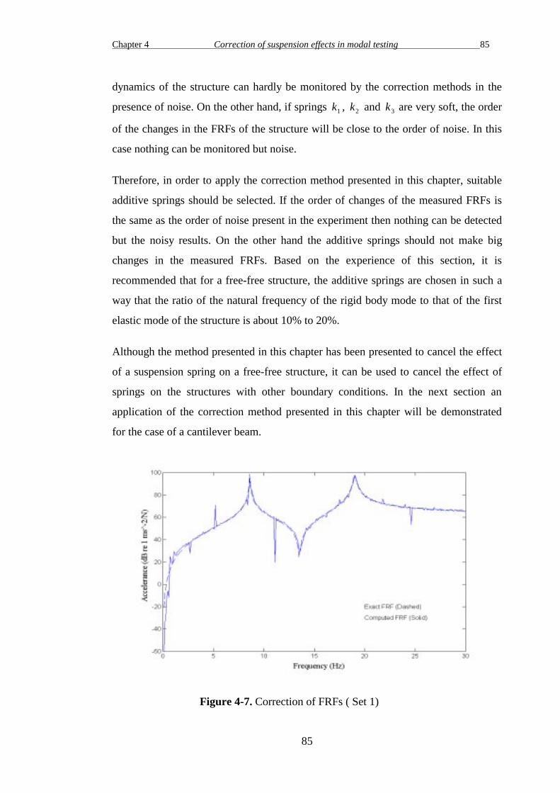
Chapter 4 Correction of suspension effects in modal testing 85
85
dynamics of the structure can hardly be monitored by the correction methods in the
presence of noise. On the other hand, if springs k1 , k2 and k3 are very soft, the order
of the changes in the FRFs of the structure will be close to the order of noise. In this
case nothing can be monitored but noise.
Therefore, in order to apply the correction method presented in this chapter, suitable
additive springs should be selected. If the order of changes of the measured FRFs is
the same as the order of noise present in the experiment then nothing can be detected
but the noisy results. On the other hand the additive springs should not make big
changes in the measured FRFs. Based on the experience of this section, it is
recommended that for a free-free structure, the additive springs are chosen in such a
way that the ratio of the natural frequency of the rigid body mode to that of the first
elastic mode of the structure is about 10% to 20%.
Although the method presented in this chapter has been presented to cancel the effect
of a suspension spring on a free-free structure, it can be used to cancel the effect of
springs on the structures with other boundary conditions. In the next section an
application of the correction method presented in this chapter will be demonstrated
for the case of a cantilever beam.
Figure 4-7. Correction of FRFs ( Set 1)
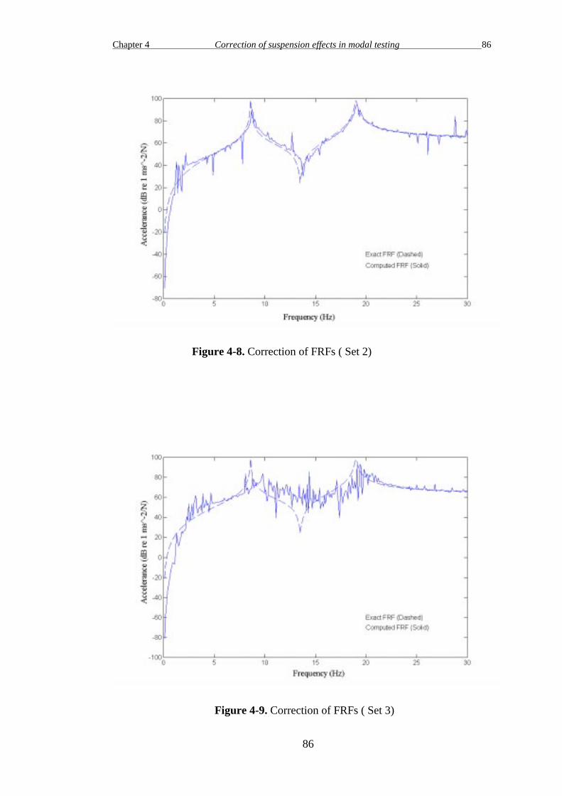
Chapter 4 Correction of suspension effects in modal testing 86
86
Figure 4-8. Correction of FRFs ( Set 2)
Figure 4-9. Correction of FRFs ( Set 3)
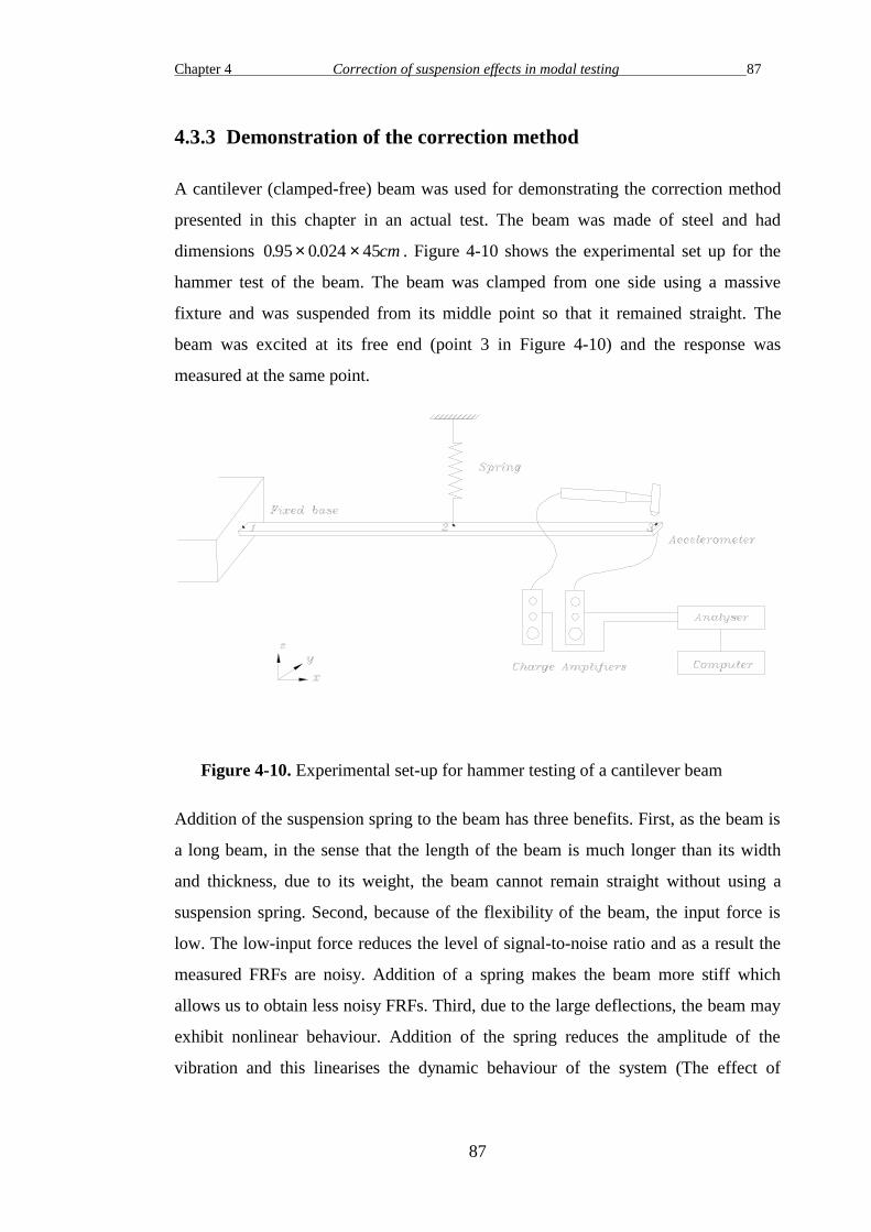
Chapter 4 Correction of suspension effects in modal testing 87
87
4.3.3 Demonstration of the correction method
A cantilever (clamped-free) beam was used for demonstrating the correction method
presented in this chapter in an actual test. The beam was made of steel and had
dimensions 0 95 0 024 45. .× × cm . Figure 4-10 shows the experimental set up for the
hammer test of the beam. The beam was clamped from one side using a massive
fixture and was suspended from its middle point so that it remained straight. The
beam was excited at its free end (point 3 in Figure 4-10) and the response was
measured at the same point.
Figure 4-10. Experimental set-up for hammer testing of a cantilever beam
Addition of the suspension spring to the beam has three benefits. First, as the beam is
a long beam, in the sense that the length of the beam is much longer than its width
and thickness, due to its weight, the beam cannot remain straight without using a
suspension spring. Second, because of the flexibility of the beam, the input force is
low. The low-input force reduces the level of signal-to-noise ratio and as a result the
measured FRFs are noisy. Addition of a spring makes the beam more stiff which
allows us to obtain less noisy FRFs. Third, due to the large deflections, the beam may
exhibit nonlinear behaviour. Addition of the spring reduces the amplitude of the
vibration and this linearises the dynamic behaviour of the system (The effect of
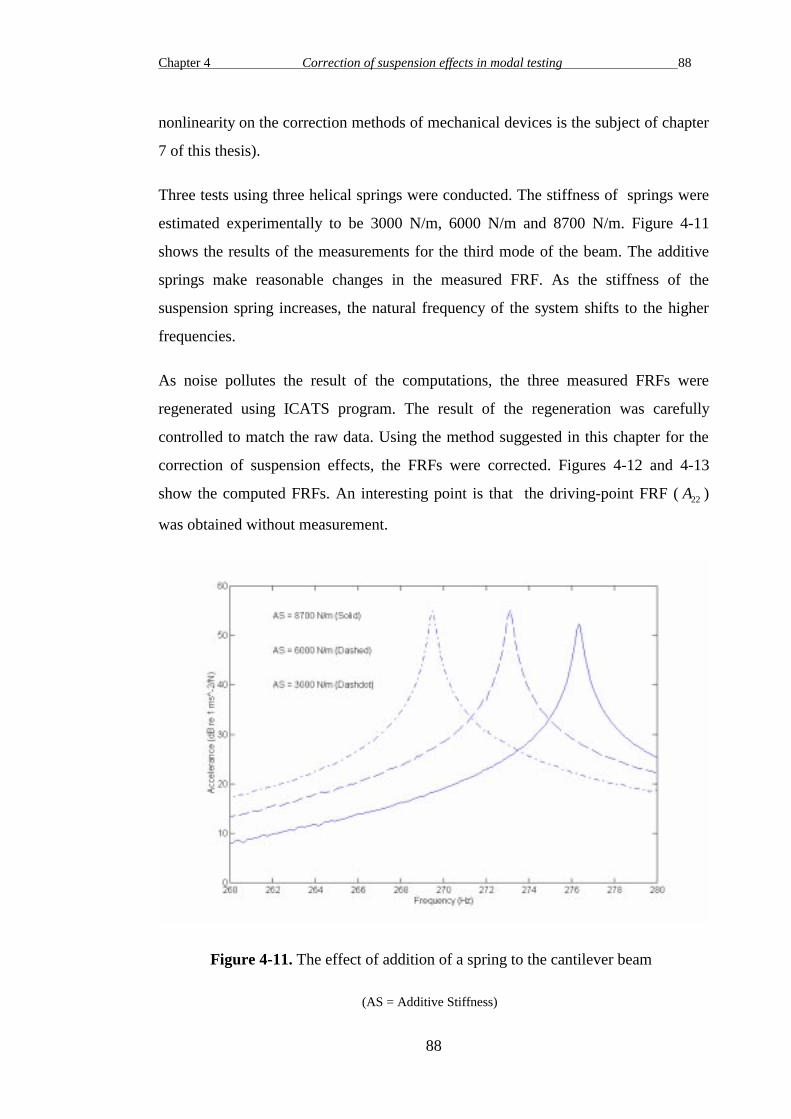
Chapter 4 Correction of suspension effects in modal testing 88
88
nonlinearity on the correction methods of mechanical devices is the subject of chapter
7 of this thesis).
Three tests using three helical springs were conducted. The stiffness of springs were
estimated experimentally to be 3000 N/m, 6000 N/m and 8700 N/m. Figure 4-11
shows the results of the measurements for the third mode of the beam. The additive
springs make reasonable changes in the measured FRF. As the stiffness of the
suspension spring increases, the natural frequency of the system shifts to the higher
frequencies.
As noise pollutes the result of the computations, the three measured FRFs were
regenerated using ICATS program. The result of the regeneration was carefully
controlled to match the raw data. Using the method suggested in this chapter for the
correction of suspension effects, the FRFs were corrected. Figures 4-12 and 4-13
show the computed FRFs. An interesting point is that the driving-point FRF ( A22 )
was obtained without measurement.
Figure 4-11. The effect of addition of a spring to the cantilever beam
(AS = Additive Stiffness)

Chapter 4 Correction of suspension effects in modal testing 89
89
Figure 4-12. Computed FRF A33
Figure 4-13. Computed FRF A22

Chapter 4 Correction of suspension effects in modal testing 90
90
In the next stage we moved the accelerometer to point 2 (see Figure 4-10) and
measured A232( ) using the spring with the stiffness of 6000 N/m, the exact FRF A23
was computed from:
AA
Ak
232 23
22
2( ) =
−ω
(4-29)
As A22 was computed already, A23 could be obtained using only one measurement.
One way of assessing the success of the method is to conduct an internal check of the
computed FRFs using their modal constants. In principle, the following equation
should hold between the modal constants of the measured FRFs of the beam:
3 333 23
2
3 22
AAA
=( )
(4-30)
where r jkA is the modal constant for mode r and coordinates j and k. On this basis
the required FRFs for equation (4-30) were regenerated and their modal constants
derived using the ICATS program. The modal constant for A33 was obtained 62.78,
for A22 was obtained 23.33 and for A23 was obtained 37.15. The result of the
calculation for the right hand side of equation (4-30) is 59.16 which is close to 62.78
for the left hand side. The result of this experiment show that the two sides of
equation (4-30) above are close together, demonstrating that the method is valid and
applicable.
4.4 Assessment of the quality of the measurement of a free-free
structure
In conventional modal testing, test structures are usually suspended using soft springs
to approximate free-free boundary conditions and, as a result, the effects of these
mechanical devices on the measured FRFs are considered negligible. In this section a
method will be suggested for assessing the quality of the measurements related to the
suspension effects. Here the emphasis is to use the theory presented earlier in this
chapter for the correction of suspension effects on the measured FRFs.

Chapter 4 Correction of suspension effects in modal testing 91
91
4.4.1 Assessment of the quality of measurement based on the
changes in the natural frequencies of the structure
As shown in section 4.2.2 when the structure is suspended from a point, the effect of
the suspension spring on the measured FRFs can be corrected using equation (4-19).
In this case the frequencies that make the determinant of the matrix:
− − −
− − −
ω
ω
2
2 1
2
3 1
1 1
1 1
( )
( )
( ) ( )
( )( )
k kA A
k kA A
lij
lij
lij
li
j (4-31)
equal to zero are the exact natural frequencies of the structure. A comparison between
the natural frequencies of the modified structure and the exact natural frequencies of
the structure can show us the quality of the measurement. However, measurement of
the structure three times using a different suspension spring in each test is a time-
consuming process. In this case the following approximate method is suggested to
reduce the number of required measurements for assessing the quality of the
measurement:
In equation (4-8), the frequencies that make the denominator, 1 1k jj+ α , equal to zero
give us the natural frequencies of the modified structure. This means that the natural
frequencies of the modified structure are at the frequencies where:
1
1α ωjj
k( )
= − (4-32)
Figure 4-14 shows a typical linear graph of the inverse of the driving point receptance
( or the dynamic stiffness ) of a point on a beam in the region of one of the modes of
the beam. At 871.6 Hz the dynamic stiffness of the beam is equal to zero which is the
natural frequency of the beam. In the frequency range of 871.6-1600 Hz the dynamic
stiffness of the beam is negative. Therefore, when a spring is attached to the beam at
this point, according to equation (4-32), the new natural frequency of the modified

Chapter 4 Correction of suspension effects in modal testing 92
92
beam is a frequency point in the range of 871.6-1600 Hz where the magnitude of the
dynamic stiffness of the beam is equal to the stiffness of the suspension spring.
Figure 4-14. The linear graph of the inverse of the receptance around one of the
natural frequencies of a beam
Figure 4-15 shows the change in the natural frequency of a structure when the
structure is modified by a suspension spring with the stiffness of k1 . In this case the
natural frequency of the structure shifts from f 0 to f1 . If the structure is suspended
using another spring with the stiffness of k2 , where k k2 12= , the resonance of the
structure shifts to f 2 .
From the geometry of triangle ABD we have:
BC
CD
AF
DF
AE
BE= = = 1 (4-33)
or:
BC=CD (4-34)

Chapter 4 Correction of suspension effects in modal testing 93
93
We have:
BC f f= −2 1 (4-35)
As we get closer to the natural frequency of the structure, the behaviour of the
dynamic stiffness of the beam becomes more linear. This means that if the structure is
suspended using very soft spring, point D (in figure 4-15) become closer to the natural
frequency of the structure, f 0 , and from relation (4-34) we have:
f f f f2 1 1 0− ≈ − ( 4-36)
However, as the stiffness of the suspension spring increases two sides of equation (4-
36) differ more. This can be seen from Figure 4-15.
Figure 4-15. Estimation of the changes in the natural frequency of a suspended
structure
This means if by doubling the stiffness of the suspension spring the natural frequency
of the modified structure does not change discernibly, two sides of equation 4-36 are
almost the same and the difference between f 2 and f1 can monitor the quality of the
measurement. Conversely, when by doubling the stiffness of the suspension spring the
natural frequency of the structure has a discernible change, two sides of equation (4-
36) are not the same but we can conclude that f1 and f 0 differ considerably as well.

Chapter 4 Correction of suspension effects in modal testing 94
94
Therefore we can assess the quality of the measurement by doubling the stiffness of
the suspension spring
4.4.2 Numerical example
The theoretical model of a beam was considered for the numerical validation of the
method presented in the last section. The theoretical model of the beam was built by
coupling of four free-free beam elements (Chapter 3). The beam was made of steel
and had dimensions of 2 0 6 44× ×. cm . A suspension spring was attached to the
middle of the beam by addition of a stiffness to the impedance matrix of the
theoretical model of the beam (Figure 4-16). In the simulated test, the beam was
excited at point 2 and the response was measured at point 4.
Figure 4-16. Assessment of the suspension effect by doubling the sttiffness of the
spring
Table 4-4 shows the application of the method presented in the previous section for
different suspension springs. As was proven when f f2 1− is small, it is equal to
f f1 0− . However, as the stiffness of the suspension spring increases f f2 1− and
f f1 0− differ more. It can be concluded that for the first suspension spring (K=1000
N/m) f f1 0− is negligible and the quality of the measurement is acceptable but for the
second and third suspension springs (K= 10000 and 20000 N/m) f f2 1− and f f1 0−

Chapter 4 Correction of suspension effects in modal testing 95
95
are not negligible and the quality of the measurement is not good. Therefore, f f2 1−
can monitor the quality of the measurement.
Table 4-4. Assessment of the suspension effect on the quality of the measurement
K (N/m) f 1 (Hz) f 2 (Hz) f f2 1− (Hz) f f1 0− (Hz)
1000 873.11 874.62 1.51 1.51
10000 886.65 903.77 17.09 15.08
20000 903.77 941.9 38.13 32.17
f 0 = Natural frequency of the structure (871.6 Hz)
f1 = Natural frequency of the structure and a suspension spring with the stiffness of K
f 2 = Natural frequency of the structure and a suspension spring with the stiffness of 2K
K = Stiffness of the suspension spring
4.4.3 Experimental case study
Figure 3-20 shows an experimental set up of shaker testing of a beam which was used
in chapter 3 for assessing of the mass-loading effect of an accelerometer. This way of
suspending the test structure for shaker testing is quite popular. The beam was
suspended using an elastic cord with the stiffness of 220 N/m and zero-load length of
10 cm. Although the elastic cord is used to offset the vertical load caused by the
weight of the beam, it exhibits a stiffness effect as well when the tip of the beam is
moved laterally. The equivalent lateral stiffness can be calculated in terms of the axial
stiffness of the elastic cord if we assume:
1. The tip of the beam experiences only horizontal motion;

Chapter 4 Correction of suspension effects in modal testing 96
96
2. The elastic cord has no mass and remains in a straight line connecting the cord
clamp and the tip of the beam;
3. The deflections of the tip of the beam are small enough such that the additional
elongation does not significantly change the tension of the elastic cord; and
4. The elastic cord behaves as a linear spring.
As shown in [42], the equivalent lateral stiffness can be calculated from:
kW
l W k
W
llatst
o st ver
st
f
=+
= (4-37)
where klat is the elastic cord lateral stiffness, kver is the elastic cord axial stiffness,
Wst is the weight of the structure, lo is the zero-load elastic cord length and lf is the
elastic cord length under load. Therefore in this way of suspending the structure not
only the axial stiffness of the suspension spring is important but its length is also
important. The axial stiffness of an elastic cord can be computed from:
kE A
lver
sp sp
o
= (4-38)

Chapter 4 Correction of suspension effects in modal testing 97
97
where Esp is the elastic modulus of the elastic cord and Asp is the cross sectional area
of the elastic cord. Equation (4-38) shows that if we divide the zero-load length of the
elastic cord in two, its axial stiffness becomes twice. Moreover, equation (4-37)
shows that in the latter case the lateral stiffness of the elastic cord becomes twice as
well because the zero-load length is half and the axial stiffness is twice. This suggests
that in order to check the quality of the measurement related to suspension effects we
have to remeasure the test structure using another suspension spring with the same
parameters but half the length of the original suspension spring (Figure 4-17). This
was done for the test case shown in Figure 3-20 and no discernible change was
detected for the first four natural frequencies of the beam ( 167 Hz, 445 Hz, 880 Hz,
1445 Hz). The lateral stiffness of the elastic cord was calculated to be 59 N/m which
is quite small. Therefore it was concluded that the measured FRF has a good quality
with respect to the suspension effects.
Figure 4-17. Assessment of the lateral stiffness of an elastic cord
Chapter 4 Correction of suspension effects in modal testing 98
98
4.4.4 Recommended test strategy
Clearly a softer suspension spring has less effect on the measurement. However, the
suspension spring should be stiff enough to stand the gravity load of the test structure.
After choosing a suitable suspension spring, the following procedure is suggested for
dealing with the suspension effect in the test:
1- Suspend the structure with the chosen spring and measure an FRF.
2- Suspend the structure with another spring with twice the stiffness of the first
spring and measure the same FRF.
3- If the difference between the natural frequencies of two measured FRFs in steps 1
and 2 are very small for a mode of the structure, the change of the natural
frequency of the structure due to the suspension effect is negligible and the quality
of the measurement is acceptable; if the difference is large the measured FRF is
not acceptable.
When the quality of the measurement relating to the suspension effects is not
acceptable two ways can be followed to improve the quality of the measurement:
1- Suspend the structure from another point of the structure. For a particular mode, if
the structure is suspended from the nodal point of the structure, the effect of the
spring on the test structure is eliminated in that mode.
2- Use the correction method presented in this chapter.
4.5 Conclusions
• In this chapter we have presented a method for the correction of the suspension
effects on test structures. It has been shown that if three different modal tests are
performed using a different suspension spring in each test, the FRFs can be
corrected.

Chapter 4 Correction of suspension effects in modal testing 99
99
• Application of the method to a numerical example of a 3 DOFs system which is
affected by suspension spring has also been examined. Moreover, the method was
successfully applied to experimental data from testing a cantilever beam.
• The method has been developed for the case where the test structure is suspended
with two springs. It has been shown that the measured FRFs can be corrected in a
step by step procedure.
• The effects of the rigid body modes on the measured FRFs have been examined
and it is shown that they are cancelled through the correction process.
• The method is vulnerable to noise and it is necessary that suitable springs are
chosen to reduce the effect of the noise.
• The quality of the measurement of a free-free structure can be assessed by
doubling the suspension stiffness and comparing the natural frequencies of the
modified structure in each test. The method was applied to experimental data from
testing on a beam which was suspended vertically using an elastic cord.

Chapter 5 The effects of stingers on measured FRFs 100
100
Chapter 5
The effects of stingers on measured FRFs
5.1 Introduction
When using a shaker to excite a structure and to measure Frequency Response
Functions, it is customary to put a stinger ( push rod or drive-rod ) between the shaker
and the force transducer which is attached to the test structure ( Figure 5-1 ) . Ideally,
the stinger should have high axial stiffness but low lateral or bending stiffness so as to
excite the structure axially and to minimise excitations in all the other DOFs.
However, forces and moments other than the axial excitation force component may
also be introduced and act on the test structure and influence the force and/or response
measurements. This will cause a systematic error in the measurement. There are
relatively few publications which quantify the effects of stingers on the measured
FRFs and the selection of stingers is usually made by trial and error or by experience.
In this chapter the effects of stingers on the measured FRFs will be investigated. The
SMURF method is used to calculate the major influence of the stinger and the test
structure on the measured results.
Figure 5-1. Shaker-structure Interaction
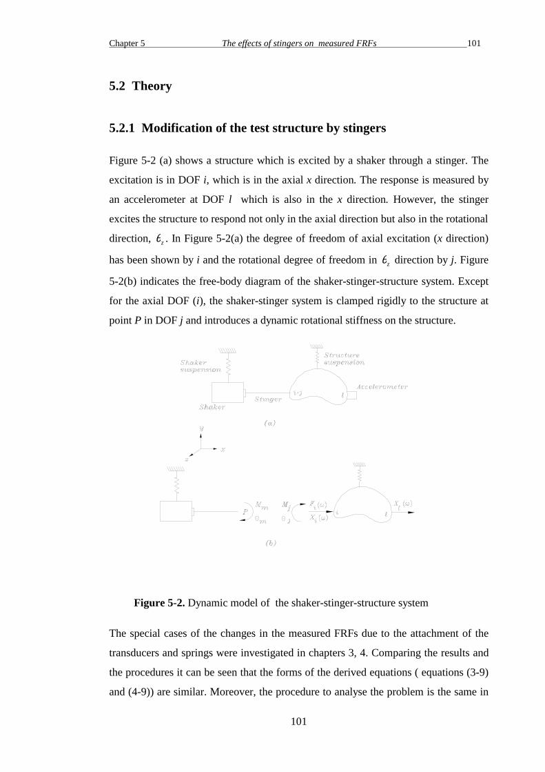
Chapter 5 The effects of stingers on measured FRFs 101
101
5.2 Theory
5.2.1 Modification of the test structure by stingers
Figure 5-2 (a) shows a structure which is excited by a shaker through a stinger. The
excitation is in DOF i, which is in the axial x direction. The response is measured by
an accelerometer at DOF l which is also in the x direction. However, the stinger
excites the structure to respond not only in the axial direction but also in the rotational
direction, θz . In Figure 5-2(a) the degree of freedom of axial excitation (x direction)
has been shown by i and the rotational degree of freedom in θz direction by j. Figure
5-2(b) indicates the free-body diagram of the shaker-stinger-structure system. Except
for the axial DOF (i), the shaker-stinger system is clamped rigidly to the structure at
point P in DOF j and introduces a dynamic rotational stiffness on the structure.
Figure 5-2. Dynamic model of the shaker-stinger-structure system
The special cases of the changes in the measured FRFs due to the attachment of the
transducers and springs were investigated in chapters 3, 4. Comparing the results and
the procedures it can be seen that the forms of the derived equations ( equations (3-9)
and (4-9)) are similar. Moreover, the procedure to analyse the problem is the same in

Chapter 5 The effects of stingers on measured FRFs 102
102
these cases. It seems that the same method can be used to analyse the general case in
which the test structure is modified in more than one DOF ( rotational or translational
). Appendix A of this thesis investigates the general case of the changes in measured
FRFs due to attachment of mechanical devices to the test structure. As shown at
appendix A for the case of the stingers that the structure is modified in one DOF the
relation between receptances is:
α αα α
α αlij
li
ji lj
jj mm
( ) = −+
(5-1)
Consequently, the relation between the accelerances is:
A AA A
A Alij
li
ji lj
jj mm
( ) = −+
(5-2)
in which j and m are rotational DOFs while i and l are translational DOFs. Alij( ) is
the measured FRF when the stinger is rigidly connected to the test structure at
rotational DOF j. Amm is the rotational receptance of the tip of the stinger at point P in
Figure 5-2.
What we want to measure is Ali , but what we get is a combination of Ali and the other
FRFs. If the shaker is connected directly to the structure (without a stinger), Amm is
close to zero and we measure :
A AA A
Alij
li
ji lj
jj
( ) = −(5-3)
In this case the structure is coupled rigidly to the shaker at DOF j and the result is
seriously contaminated.
In equation (5-2) when Amm is large, the amount of the fraction on the right hand side
is small and consequently the measured FRF is close to Ali . Conversely, when Amm is
small, the amount of error is large. In other words, when the stinger is dynamically
stiff at any area of the frequency range, the measured results are more vulnerable to

Chapter 5 The effects of stingers on measured FRFs 103
103
error in that area. Hence, this suggests that the antiresonances of the rotational
driving point receptance of the tip of the stinger are responsible for the maximum
error in measured FRFs. This question remains as to how we can deal with these
undesirable effects and this will be discussed below.
5.2.2 Feasibility of correction of the stinger effects
Correction of FRFs for the case of stingers is similar to the case of springs discussed
in chapter 4 because the form of the governing equation is the same for both cases
(Equations (4-9) and (5-2)). Equation (5-2) shows how the measured translational
FRF, Alij( ) , is related to the exact FRFs, Ali , Aji , Ajj and Alj . To find the exact
FRF, measurement of Alij( ) can be considered with three different stingers with
different lengths (Figure 5-3). So there are three equations in the form of equation (5-
2) corresponding to three different stingers.
Figure 5-3. Measurement with three different stingers
A AA A
A A
A AA A
A A
A AA A
A A
lij
li
ji lj
jj mm
lij
li
ji lj
jj mm
li
j
li
ji lj
jj mm
( )
( )
( )
= −+
= −+
= −+
(5-4)

Chapter 5 The effects of stingers on measured FRFs 104
104
in which Amm , Amm and Amm are rotational FRFs of the stingers at point P. If Amm ,
Amm and Amm are known, the correct values of Ali and Ajj can be computed. The
solution of the general form of these equations can be found in chapter 4. For the case
of equations (5-4), the solutions are :
A
AA A A A
A A A A
A A A A
A A A A
li
jj
mm mm lij
lij
mm mm lij
li
jli
jmm li
jmm
li
j
mm lij
mm
=− −
− −
−
−
−( ) ( )
( )( )
( ) ( )
( )( )
( )
( )
1
(5-5)
Thus, the correct FRF, Ali , and the rotational driving point FRF at the point of
attachment of the stinger, Ajj , have been computed with respect to measured FRFs
and Amm ’s, namely the rotational point accelerances at point P of the stingers (Figure
5-2(b)). However, measurement of Amm is not as straightforward as measuring the
mass of the accelerometer in the mass cancellation procedure. Measurement of the
rotations of such a small elements as stingers is not an easy task . Theoretical results
to compute Amm is not exact as well because the shaker-stinger assembly is a
complicated structure some part of which (the coil) is moving in a magnetic field and
any simplification in the theoretical model will lead to inaccurate results from the
correction methods. Thus the correction method for the case of stingers is ineffective.
5.3 The effects of stingers on measured FRFs
In the previous section, it was explained that the correction of the rotational stiffness
effect of stingers on the measured FRFs is an impractical task because measurement
or exact simulation of the behaviour of stingers is impractical. However, the
behaviour of stingers can be simulated approximately using simplified models of
shaker-stinger assembly. On this basis stingers can be designed in a way that their
effect on the measured FRFs is minimised. In this section practical ways to avoid the
effects of stingers on the measured FRFs will be investigated.

Chapter 5 The effects of stingers on measured FRFs 105
105
5.3.1 Shaker-stinger-structure model
As was explained in chapter 2 different models were suggested in the past for the
shaker-stinger-structure assembly ( Figures 2-1 and 2-2 ) by different authors [17],
[18], [19]. However, the dynamic characteristics of the test structure were not
included in these models and it was simply assumed that the structure-side boundary
condition of the stinger was pinned or clamped. Figure 5-4 indicates a more complete
model of the shaker-stinger-structure system in which the test structure is considered
as a rigid structure that moves in the transverse direction (relative to the excitation
direction) . The stinger is modelled as a simple straight beam and the mass and
suspension properties of the structure are coupled to the stinger in the transverse
direction to illustrate the effect of the boundary conditions of the stinger on the
structure side. This assumption for the transverse motion of the structure as a rigid
body does not contradict with the axial vibration of the structure as a elastic body.
Figure 5-4. Shaker-stinger-structure model
The theoretical model of the shaker-stinger-structure system shown in Figure 5-4 is
built on the concept of the coupling method. The shaker is modelled as a member
with both a specified point mass and a point rotational inertia and the suspension of
the shaker is modelled as a translational stiffness and a rotational stiffness. In reality,
the stinger is coupled with the coil of the shaker which is moving in the magnetic
field of the drive part of the shaker. However, this cannot be modelled by mechanical
elements. The shaker can be modelled as shown in Figure 5-5. Because the coil has a
slight axial motion, the rotational inertia properties of the shaker do not change

Chapter 5 The effects of stingers on measured FRFs 106
106
considerably. Hence, the shaker can be modelled as a lumped mass with rotational
inertia as is shown in Figure 5-4.
Figure 5-5. A model of the shaker
The separate stinger was assumed to be a free-free beam of constant cross-section
which is modelled using the receptance function of a free-free beam introduced in
[96]. The receptance matrix of the stinger (see Figure 5-6) is:
[ ]α
α α α αα α α αα α α αα α α α
=
q q q r q q q r
r q r r r q r r
q q q r q q q r
r q r r r q r r
Sh Sh Sh Sh Sh St Sh St
Sh Sh Sh Sh Sh St Sh St
St Sh St Sh St St St St
St Sh St Sh St St St St
(5-6)
in which q qSh St, and r rSh St, are the vertical and rotational displacements of two sides
of the stinger.
Figure 5-6. Modelling of a stinger as a free-free beam
The elements of [ ]α can be computed with respect to the beam properties as given in
[96]. To complete the model of the shaker-stinger-structure system, the dynamic
characteristics of the shaker and those of the structure should be added to the stinger
as its two ends.
The mass of the shaker and the linear stiffness of the shaker suspension are added to
the stinger as :
D q q D q q m kmdSh Sh Sh Sh sh sh( , ) ( , )= − +ω 2 (5-7)

Chapter 5 The effects of stingers on measured FRFs 107
107
The rotary moment of inertia of the shaker and the rotational stiffness of the shaker
suspension are added to the stinger as :
D r r D r r I krmdSh Sh Sh Sh sh sh( , ) ( , )= − +ω 2 (5-8)
Moreover, the mass and suspension stiffness of the structure are added to the structure
side of the stinger as:
D q q D q q m kmdSt St St St st st( , ) ( , )= − +ω 2 (5-9)
Thus the modified receptance matrix of the stinger is :
[ ] [ ]α md mdD= −( ) 1 (5-10)
5.3.2 Comparison of different models of the stinger
The model shown in Figure 5-4 is not a simple model of the stinger and it has some of
the parameters involved in the real test ( this model is called real model from now on
). However, for simplification purposes it is valuable to compare this model with the
simpler models of stingers such as the ones shown in Figure 5-7.
Figure 5-7. Three simple models for a stinger

Chapter 5 The effects of stingers on measured FRFs 108
108
To compare these models with the “real model”, a numerical simulation was
considered. The parameters of the shaker, stinger and the structure are :
Shaker : Mass : 8.3 kg; Rotary moment of inertia : 0.0256 kg m/ 2 , Suspension: ksh =
1400 N/m, krsh = 0.469 N-m/rad.
Stinger : Diameter : 2 mm, Length : 100 mm, Material : steel
Structure : a beam with the mass of mst =2.469 kg and the suspension stiffness of
kst =850 N/m.
Table 5-1 shows a comparison of the natural frequencies and antiresonance
frequencies of the receptance function of point l of the model of the stinger shown in
Figure 5-4 with those of the three simple models shown in Figure 5-7. The
measurement points are specified as A in Figure 5-7. In this case, the resonances and
antiresonances of the real model coincide with those of the clamped-pinned model.
This means the stinger can be modelled using a clamped-pinned model.
Table 5-1. Comparison of different models of the stinger
Model of the beam Natural Frequencies / Antiresonances (Hz)
AR of the RM of beam 934 2574.9 5047.7 8344.2
AR of the CP beam 934 2574.9 5047.7 8344.2
NF of the FF beam 934 2574.9 5047.7 8344.2
NF of the CF beam 146.8 934 2574.9 5047.7 8344.2
NF of the RM of beam 643.7 2086 4352.4 7442.8
NF of the CP beam 643.7 2086 4352.4 7442.8
AR= AntiResonance, RM= Real Model, CP= Clamped-Pinned, NF= Natural Frequency,
FF= Free-Free, CF= Clamped-Free.

Chapter 5 The effects of stingers on measured FRFs 109
109
Some researchers advise that to minimise the effect of stinger on the measured FRFs
the resonance frequencies of the stinger should lie below or above the frequency range
of measurement [17], [18], [19], [20], while others claim that this is the antiresonance
of the stinger that is responsible for the maximum error [21]. It was shown in section
9-2 that in coupling the shaker-stinger assembly with the structure, it is the
antiresonance of the stinger’s angular driving point receptance which is responsible
for the maximum error. However, as can be seen in Table 5-1, the antiresonances of
the clamped-pinned stinger coincide with the natural frequencies of the free-free
stinger and the natural frequencies of the clamped-free stinger (except for the first
resonance). This coincidence can be proven as follows:
In Table 7.1( c ) of [96] entries 1 and 3 it is shown that the rotational point receptance
of the tip of a beam for the free-free and clamped-free boundary conditions
respectively are F EI F6 3( )λ and F EI F3 5( )λ , in which λ is a function of frequency,
cross section area of the beam, mass density and flexural rigidity of the beam. F3 , F5
andF6 are functions of λ and the length of the beam. F3 is in the denominator of the
free-free condition and in the numerator of the clamped-pinned condition. It means
that when the receptance of the clamped-pinned beam is zero ( or in anti-resonance ),
the receptance of the free-free beam is ∞ ( or in resonance ). Moreover, As shown in
[97] in Table 8-1, the natural frequencies of the free-free beam, clamped-clamped
beam and clamped-free beam ( except for the first one ) are the same. It is a
considerable result when we remember that most programs today are calculating
natural frequencies and not antiresonances.
Table 5-2 indicates the antiresonances of the clamped-pinned stingers with different
diameters and lengths. These are the lengths and diameters which usually are used in
modal testing. The material of the stinger is steel. When using these stingers, the
measurement may be affected around antiresonances of the stinger. The regions
between these antiresonances are safe regions for the measurement.
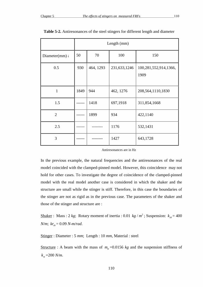
Chapter 5 The effects of stingers on measured FRFs 110
110
Table 5-2. Antiresonances of the steel stingers for different length and diameter
Length (mm)
Diameter(mm)↓ 50 70 100 150
0.5 930 464, 1293 231,633,1246 100,281,552,914,1366,
1909
1 1849 944 462, 1276 208,564,1110,1830
1.5 ------ 1418 697,1918 311,854,1668
2 ------ 1899 934 422,1140
2.5 ------ -------- 1176 532,1431
3 ------ -------- 1427 643,1728
Antiresonances are in Hz
In the previous example, the natural frequencies and the antiresonances of the real
model coincided with the clamped-pinned model. However, this coincidence may not
hold for other cases. To investigate the degree of coincidence of the clamped-pinned
model with the real model another case is considered in which the shaker and the
structure are small while the stinger is stiff. Therefore, in this case the boundaries of
the stinger are not as rigid as in the previous case. The parameters of the shaker and
those of the stinger and structure are :
Shaker : Mass : 2 kg; Rotary moment of inertia : 0.01 kg m/ 2 ; Suspension: ksh = 400
N/m; krsh = 0.09 N-m/rad.
Stinger : Diameter : 5 mm; Length : 10 mm, Material : steel
Structure : A beam with the mass of mst =0.0156 kg and the suspension stiffness of
kst =200 N/m.

Chapter 5 The effects of stingers on measured FRFs 111
111
Figure 5-8 shows the comparison of the real model with the clamped-pinned and
clamped-free models. In this case, the structure and shaker are not so massive while
the stinger is not flexible but the real model is still close to the clamped-pinned
model. It should be mentioned that the real model show the effect of the rigid body
modes of the shaker-stinger-structure system in the frequency range of 0-500 Hz
while the clamped-pinned model does not show this.
Figure 5-8. Measurement of a small structure using a small shaker and a stiff stinger
5.3.3 The effects of the stinger on the rigid body modes
The rigid body modes of the shaker-stinger-structure system have considerable effects
on the measured FRFs in the low frequency range. By “low frequency range” we
mean the frequency range in which the minimum frequency is zero and the maximum
frequency is the first elastic mode of the shaker-stinger-structure system shown in
Figure 5-4. The additional stiffness of the stinger (rotational and transverse) an raise
the rigid body modes of the shaker and those of the structure in the low frequency
range ( like the effect of the suspension springs on the rigid body modes of a test
structure). Figure 5-9 indicates the effects of different stingers on the rigid body

Chapter 5 The effects of stingers on measured FRFs 112
112
modes of the shaker-stinger-structure system. The parameters of the system used in
this example are:
Shaker : Mass : 8.3 kg, Rotary moment of inertia : 0.0256 kg m/ 2 , Suspension: ksh =
1400 N/m, krsh = 0.469 N-m/rad.
Structure : is a beam with the mass of mst =2.469 kg and its suspension stiffness is
kst =850 N/m.
Three different stingers were considered from steel:
Stinger 1 : Diameter : 2 mm ; Length : 100 mm.
Stinger 2 : Diameter : 0.5 mm ; Length : 100 mm.
Stinger 3 : Diameter : 2 mm ; Length : 50 mm.
Three resonances and three antiresonances are found in the angular receptance of the
tip of the stinger (Point P in Figure 5-2) in the frequency range of 0 to 20 Hz for
stinger 1. As was explained in section 5.2.1, the antiresonances of the stinger are
responsible for the maximum error in the measured FRFs. For a shorter stinger with
the same diameter (stinger 3), the antiresonances and resonances shift to the higher
frequencies. This means that a shorter stinger raises the rigid body mode frequencies
in the low frequency range. For stinger 2, which is thinner than stinger 1 but with the
same length, the rigid body mode frequencies shift to the lower frequencies.
Comparing these three stingers, stinger 2 has less effect on the rigid body modes in
the low frequency range. Therefore, in order to measure the test structure at lower
frequencies the stinger should be thinner and longer or, in other words, more flexible.
In design of stingers we usually ignore the results of the measurement in the
frequency range from zero to the last antiresonance in the low frequency range.
Therefore what is important in the low frequency range is the last antiresonance of the
shaker-stinger-structure system. For the above-mentioned example, computations
show that by changing the parameters of the shaker and the suspension stiffness of the
structure, the location of the last antiresonance in the low frequency range does not

Chapter 5 The effects of stingers on measured FRFs 113
113
change considerably. In other words the important parameters in the design of stingers
in the low frequency range are the parameters of the stinger and the mass of the
structure.
Figure 5-9. The effect of the stingers on the rigid body modes in the low frequency
range
5.3.4 The effects of the flexibility of stinger on the measured FRFs
The rigid body modes of the shaker-stinger-structure system affect the measured FRFs
in the low frequency range. A common problem that is encountered in the higher
frequency region is the flexibility of the stinger. As was explained in section 5.2.1, at
antiresonances of the rotational point receptance function of the tip of the stinger, the
stinger is dynamically stiff and the measured FRFs will be more erroneous at these
frequencies compared with other frequencies. Figure 5-10 indicates the rotational
receptance of stingers for different diameters and different lengths. The parameters of
the stingers are given in Table 5-3. The parameters of the shaker and those of the
structure are :
Shaker : Mass : 8.3 kg, Rotary moment of inertia : 0.0256 kg m/ 2 , Suspension:
ksh = 1400 N/m, krsh = 0.469 N-m/rad.
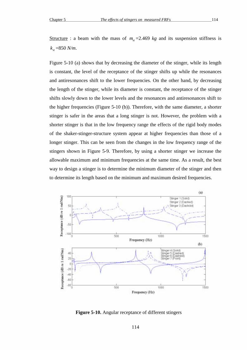
Chapter 5 The effects of stingers on measured FRFs 114
114
Structure : a beam with the mass of mst =2.469 kg and its suspension stiffness is
kst =850 N/m.
Figure 5-10 (a) shows that by decreasing the diameter of the stinger, while its length
is constant, the level of the receptance of the stinger shifts up while the resonances
and antiresonances shift to the lower frequencies. On the other hand, by decreasing
the length of the stinger, while its diameter is constant, the receptance of the stinger
shifts slowly down to the lower levels and the resonances and antiresonances shift to
the higher frequencies (Figure 5-10 (b)). Therefore, with the same diameter, a shorter
stinger is safer in the areas that a long stinger is not. However, the problem with a
shorter stinger is that in the low frequency range the effects of the rigid body modes
of the shaker-stinger-structure system appear at higher frequencies than those of a
longer stinger. This can be seen from the changes in the low frequency range of the
stingers shown in Figure 5-9. Therefore, by using a shorter stinger we increase the
allowable maximum and minimum frequencies at the same time. As a result, the best
way to design a stinger is to determine the minimum diameter of the stinger and then
to determine its length based on the minimum and maximum desired frequencies.
Figure 5-10. Angular receptance of different stingers

Chapter 5 The effects of stingers on measured FRFs 115
115
Table 5-3. The parameters of different stingers
Stinger No.1 No.2 No.3 No.4 No.5 No.6 No.7
Diameter (mm) 2.5 1 0.6 1 1 1 1
Length (mm) 100 100 100 120 60 61 30
5.3.5 The effect of the shaker-stinger-structure system on the
measured FRFs
In section 5-2 it was shown that the effect of the stinger on the measured FRFs can be
computed from equation (5-2). Moreover, using the model shown in Figure 5-4, it
was shown that how the rotational FRF of the tip of the beam ( Amm in equation (5-
2) ) varies and where are the most erroneous areas in the frequency range of a stinger.
In this section the effects of the shaker-stinger-structure system on the measured FRFs
of a beam as a test structure are investigated. Here, the effect of the structure as a rigid
body on the boundary conditions of the stinger in the transverse direction should not
be confused with the measurement of the elastic behaviour of the structure in the axial
direction.
As a test structure, a theoretical model of a beam is built using the concept of
coupling of the free-free beam elements. The procedure of building a model of the
beam by coupling the beam elements is explained in Chapter 3. The model of the
beam was built by coupling 10 beam elements and was used in a numerical simulation
to illustrate the effects of the shaker-stinger-structure system on the measured FRFs
(Figure 5-11). The shaker-stinger-structure system is coupled with the beam at point 4
(Figure 5-11) using equation (5-2). The response of the beam is measured at point 8.
The parameters of the beam and those of the shaker and stinger are :

Chapter 5 The effects of stingers on measured FRFs 116
116
Beam : Length : 106 mm, Width : 20 mm, Thickness : 1mm, Material: steel, Modulus
of elasticity : 2.1 × 10¹¹ N/m 2 , Mass of density : 7800 kg/m 3 , Mass : 0.0156 kg,
Suspension : kst =200 N/m.
Shaker : Mass : 2 kg, Rotary moment of inertia : 0.01 kg m/ 2 , Suspension: ksh = 400
N/m, krsh = 0.09 N-m/rad.
Stinger1 : Diameter : 1.5 mm , Length : 73.5 mm, Material : Steel.
Stinger 2 : Diameter: 0.5 mm, Legth: 50 mm, Material : Steel.
Measurement Set up : Excitation : at point 4, Response: at point 8.
Frequency range : 0-2000 Hz.
Figure 5-12(b) indicates the rotational point receptance of the structure-side end of the
stinger 1. The behaviour of the real model ( the real mode was introduced in section
5.3.1) is compared with the behaviour of the clamped-pinned stinger. Figure 5-12(a)
shows the effects of the stinger on the measurement of the beam. A “glitch” occurs in
the computed FRF in the low frequency range. At higher frequencies, a notch has
been made by the antiresonance of the shaker-stinger-structure system in the
measured FRF and thus instead of one peak a double peak has been indicated.
Moreover, because of the high angular stiffness of the stinger , around 450 Hz , the
FRF has moved to the higher frequencies.
Figure 5-11. Measurement of a beam in a simulated test

Chapter 5 The effects of stingers on measured FRFs 117
117
Figure 5-12. Measurement using stinger 1 : ds =0.0015 m, ls =0.0735 m.
Figure 5-13 (b) indicates the angular receptance of the structure-side end of stinger 2.
Figure 5-13 (a) shows the effects of stinger 2 on the measured FRF. This stinger has a
small effect on the resonances of the structure. Besides, in the low frequency range
the stinger has a small effect on the structure.
Figure 5-13. Measurement using stinger 2 : ds =0.0005 m, ls =0.05 m

Chapter 5 The effects of stingers on measured FRFs 118
118
From this study it can be concluded that the measured FRFs:
1. are affected by the rigid body modes of the shaker-stinger-structure system at low
frequency region;
2. are affected by the antiresonances of the stinger at higher frequencies;
3. may be affected by the rotational stiffness of the stinger at all the other
frequencies if the stinger is not flexible.
5.3.6 The effect of the misalignment on the performance of the
stinger
The main assumption of building the model shown in Figure 5-4 was that after
assembling the shaker-stinger-structure system the stinger remains straight. On this
basis the model of the stinger was assumed to be a straight beam. However, in
practice when the gravity load of the structure and that of the shaker exert tension on
the suspension springs and stretch them, in equilibrium, the stinger may not remain
straight. This causes misalignment of the stinger. Usually, the suspension springs are
chosen to be very soft to fulfil the free-free boundary condition, consequently even
with a slight force the suspension springs have a considerable displacement. This
makes it difficult to assemble the test structure and exciter accurately so that the
stinger remains straight. To examine the effect of the misalignment on the
performance of the stinger Finite Element Method (FEM) was used. Figure 5-14
shows the model which was made in ANSYS program (see Appendix D). This model
is similar to the model shown in Figure 5-4 and has the capability of assessing the
misalignment effect of stingers. The stinger was modelled by assembling 100 BEAM3
elements from ANSYS element library. BEAM3 is a uniaxial element with tension,
compression and bending capabilities. The element has three degrees of freedom at
each node: translations in the nodal x and y directions and rotation about the nodal z-
axis. The shaker is modelled as a nodal mass with rotary inertia property which is
attached to the shaker-side of the stinger. The shaker is suspended using a
longitudinal spring in y direction and a rotary spring in θz direction. On the structure

Chapter 5 The effects of stingers on measured FRFs 119
119
side, the structure is modelled as a lumped mass which is suspended using a
longitudinal spring. If the axis of the gravity force of the structure does not pass
through the point of the attachment of the stinger and the structure, the gravity force
of the structure exerts a specific moment on the stinger in the structure-side. It is
assumed that this moment can be estimated from the static properties of the structure.
Appendix D of this thesis shows the program which was used to build the ANSYS
model of the shaker-stinger-structure system. To examine this model a test with the
following parameters was considered:
Shaker : Mass : 8.3 kg; Rotary moment of inertia : 0.0256 kg m. 2 , Suspension: ksh =
1400 N/m, krsh = 0.469 N-m/rad; Mass of the coil = 0.06 kg.
Stinger : Diameter : 2 mm , Length : 100 mm, Material : steel
Structure : Mass: mst =10.5 kg and the suspension stiffness of kst =850 N/m. The
structure exerts a moment of 1.25 kg m. 2 on the stinger.
Figure 5-14. The ANSYS model of shaker-stinger-structure system
After building the model a prestressed modal analysis (this analysis is defined in the
ANSYS program) was conducted to calculate the natural frequencies and mode
shapes of the system. The procedure to do a prestressed modal analysis is essentially
the same as a regular modal analysis except that we first need to prestress the

Chapter 5 The effects of stingers on measured FRFs 120
120
structure by exerting gravity forces and doing a static analysis. Figure 5-15 shows the
result of the static analysis. In this case the stinger is deformed and is not straight any
more.
Figure 5-15. Misalignment of the stinger
In the second stage, modal analysis of the deformed system was performed by re-
entering the solution of the static analysis and obtaining the modal solution, also with
prestress effects turned on. The modal solution without performing the static analysis
was also obtained in order to compare the results. Table 5-4 compares the natural
frequencies and the mode shapes for the first fifteen modes of these two cases. The
mode shape is related to the rotation of the structure-end of the stinger. Figure 5-16
shows the mode shapes of the shaker-stinger-structure system. It was shown earlier in
section 5-2 that antiresonances of the stinger are responsible for the maximum error in
the measured FRFs, therefore the point rotational receptance of the stinger in the
structure side needs to be computed to obtain the antiresonances of the stinger. This
can be achieved using the following equation:
αϕ
ω ωlllr
rr
N
=−=
∑ ( )2
2 21
(5-11)
in which ϕlr is the mass-normalised mode shape of the point rotational receptance of
the stinger in the structure-side corresponding to mode r. Figure 5-17 shows first two
anti-resonances of the stinger using the first twenty modes of the system (Table 5-4
shows data of the first 15 modes of the system). The first antiresonance for the

Chapter 5 The effects of stingers on measured FRFs 121
121
deformed stinger is 943 Hz while for the straight stinger is 953 Hz. The second anti-
resonance for the deformed stinger is 2605 Hz while for the straight stinger is 2631
Hz. Consequently, if we do not consider the misalignment of the stinger there is a 10
Hz difference for the first anti-resonance and 26 Hz for the second anti-resonance
which is a considerable amount in the design of stingers.
Table 5-4. Comparison of the mode shapes of the straight and deformed stingers
Straight stinger Deformed Stinger
modes f (Hz) ( )θz l f (Hz) ( )θz l
1 0.0000 -0.29686E-5 0.90965 -0.11226E-8
2 1.1845 2.2958 1.842 2.2958
3 1.7978 0.26471E-1 1.7979 0.26147E-01
4 3.0326 7.2411 3.0326 7.2411
5 188.7 0.8684E-9 188.7 -0.19439E-13
6 636.58 1153.4 637.04 1155.1
7 2062.0 2015.9 2064.5 -2020.9
8 4299.4 2913.7 4335.8 -2948.4
9 7345.8 3806.6 7425.8 3864.4
10 11197 4697.0 11405 4843.6
11 15847 5584.0 16382 -5949.5
12 21289 6467.1 22255 -6506.2
13 25946 0.87009E-8 28932 8672.0
14 27516 7345.4 29327 0.94278E-8
15 34519 8218.8 39050 -9884.1
f = Natural Frequency , ( )θz l = rotation of the structure-side end of the stinger

Chapter 5 The effects of stingers on measured FRFs 122
122
Figure 5-16. Mode shapes of the shaker-stinger-structure system

Chapter 5 The effects of stingers on measured FRFs 123
123
Figure 5-17. The effect of the misalignment of the stinger on its anti-resonances
5.3.7 The effect of the stinger on the measured FRFs in other DOFs
Figure 5-18 (a) indicates a structure which is coupled with the shaker-stinger system
in three DOFs. The degree of freedom of axial excitation (x direction) has been shown
by i, the rotational degree of freedom in θz direction by j and the transverse degree of
freedom (y direction) by k. Except for the axial DOF (i), the shaker-stinger system is
coupled rigidly to the structure at point P in DOFs j and k and introduces a dynamic
stiffness on the structure.

Chapter 5 The effects of stingers on measured FRFs 124
124
Figure 5-18. Coupling of the shaker-stinger system and the structure in three DOFs
The structure and the shaker-stinger system are coupled in three DOFs. In this case
coupling can be done in a step by step procedure. In this approach two structures are
coupled in one of the coupling DOFs in each step. If it is assumed that just the effect
of the shaker-stinger system in axial direction (DOF i) is added to the structure, then
from appendix A we have:
A AA A
A Alii j k
lij k ii
j kli
j k
iij k
nn
( , , ) ( , )( , ) ( , )
( , )= −+
( 5-12)
In equation (5-1), Alij k( , ) and Aii
j k( , ) can be written in terms of the accelerances of the
structure when the effect of the shaker-stinger system in θz direction (DOF j) is
considered. For instance for Alij k( , ) we have:
A AA A
A Alij k
lik ji
klj
k
jjk
mm
( , ) ( )
( ) ( )
( )= −+
(5-13)

Chapter 5 The effects of stingers on measured FRFs 125
125
In equation (5-1), Alik( ) , Aji
k( ) , Aljk( ) and Ajj
k( ) can be written in terms of the
accelerances of the structure when the effect of the shaker-stinger system in y
direction (DOF k) is considered. For instance for Alik( ) we have:
A AA A
A Alik
liki lk
kk rr
( ) = −+
(5-14)
What we want to measure is Ali , but what we get is a combination of Ali and the other
FRFs. If the shaker is connected directly to the structure (without a stinger), Ann , Amm
and Arr are close to zero and the result is seriously contaminated.
In equation (5-1), when Ann is large, the amount of the fraction on the right hand side
is small and consequently the measured FRF is closed to Ali . Conversely, when Ann
is small, the amount of error is large. In other words, when the stinger is dynamically
stiff in the x direction at any area of the frequency range, the measured results are
more vulnerable to error in that area. This fact holds for Amm and Arr in equations (5-
13) and (5-14) as well. Hence, this suggests that the antiresonances of the driving
point FRFs of the tip of the stinger are responsible for the maximum error in
measured FRFs. It was assumed that the structure behaved as a rigid body in the
transverse direction (k DOF). Thus, we shall not consider the effect of the structure in
the transverse direction.
5.3.8 The effect of the stinger on the measured FRFs in the axial
direction
The stinger which was modelled in ANSYS by assembling BEAM3 elements has
tension and compression capability, therefore it can be used to estimate the axial
behaviour of the stinger. However, as shown in Figure 5-5, in the axial direction the
coil of the shaker slides on the drive part of the shaker. Therefore, assuming that
whole of the shaker can be modelled as a lumped mass is not valid in the axial
direction. In the previous section, Figure 5-16 shows that the fifth mode of the shaker-
stinger-structure system is in the axial direction. This is not a true axial mode because
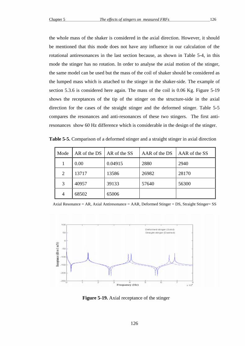
Chapter 5 The effects of stingers on measured FRFs 126
126
the whole mass of the shaker is considered in the axial direction. However, it should
be mentioned that this mode does not have any influence in our calculation of the
rotational antiresonances in the last section because, as shown in Table 5-4, in this
mode the stinger has no rotation. In order to analyse the axial motion of the stinger,
the same model can be used but the mass of the coil of shaker should be considered as
the lumped mass which is attached to the stinger in the shaker-side. The example of
section 5.3.6 is considered here again. The mass of the coil is 0.06 Kg. Figure 5-19
shows the receptances of the tip of the stinger on the structure-side in the axial
direction for the cases of the straight stinger and the deformed stinger. Table 5-5
compares the resonances and anti-resonances of these two stingers. The first anti-
resonances show 60 Hz difference which is considerable in the design of the stinger.
Table 5-5. Comparison of a deformed stinger and a straight stinger in axial direction
Mode AR of the DS AR of the SS AAR of the DS AAR of the SS
1 0.00 0.04915 2880 2940
2 13717 13586 26982 28170
3 40957 39133 57640 56300
4 68502 65006
Axial Resonance = AR, Axial Antiresonance = AAR, Deformed Stinger = DS, Straight Stinger= SS
Figure 5-19. Axial receptance of the stinger

Chapter 5 The effects of stingers on measured FRFs 127
127
5.3.9 Computation of the rigid body modes using FEM model
It was shown in section 5.3.1 that the additional stiffness of the stinger raises the rigid
body mode frequencies of the shaker and those of the structure. The ANSYS model
which was introduced in the previous section can be used to estimate the rigid body
modes of the shaker-stinger-structure system for a deformed stinger. If the structure is
assumed to behave as a rigid body then derivation of the rigid body modes is possible.
This can be done by considering a lumped mass in the structure end of the stinger
which has three DOFs in the axial, transverse and rotational directions. The mass of
the structure can easily be measured. However, the moment of inertia of the structure
is usually unknown and needs to be estimated using approximate methods. The
example of section 5.3.6 is considered here again. Table 5-6 indicates the rigid body
modes for the straight stinger and the deformed stinger. The moment of inertia of the
structure was estimated to be 0.03 kg m. 2 . It should be mentioned that for the axial
rigid body mode the mass of the coil should be considered on the shaker side. The
results of the straight stinger and the deformed stinger cases do not show too much
difference (see Table 5-6). Usually the highest rigid body mode is important to choose
the minimum allowable measurement frequency. Therefore we can use a straight
stinger model with enough accuracy for predicting the behaviour of the stinger in the
low frequency range even there is a misalignment.
Table 5-6. Rigid body modes of the shaker-stinger-structure system
No. of mode Straight stinger Deformed stinger
axial mode (1) 0.049147 0.00000
2 1.0573 1.0573
3 1.7317 1.7319
4 1.8052 1.7815
5 4.6752 4.6753
6 0.42653 0.27282

Chapter 5 The effects of stingers on measured FRFs 128
128
5.4 Experimental case study
A beam was tested in the laboratory to validate the shaker-stinger-structure model
presented in this chapter. The beam was made of mild steel, and had dimensions
0 2 0 006 0 44. . .× × m and its weight was 0.412 kg. The experimental model of the beam
was divided into 6 equal elements and was tested in a free-free configuration,
suspended vertically by a soft elastic cord attached to the beam at point 1 (see Figure
5-20). The beam was excited by a shaker at point 6 and the response was measured at
point 5 using an accelerometer with the weight of 0.004 kg. The input signal to the
power amplifier was random and Hanning windows were used in both input and
output channels to reduce the effects of the leakage. The weight of the shaker was
10.5 kg and its moment of inertia, with respect to the horizontal axis which passes
through the centre of gravity of the shaker, was estimated to be 0.03 kg m. 2 . The
weight of the accelerometer was 0.015 kg. The stiffness of the suspension spring of
the shaker was estimated experimentally to be 5400 N/m and that of the structure was
estimated to be 1200 N/m. No rotary spring was considered for the shaker because
just one spring was used to suspend it. Four different stingers were used to transfer
the excitation force of the shaker to the structure. Table 5-7 shows the parameters of
the stingers. The diameters of the stingers are the same while their lengths are
different.
Figure 5-21 shows the predicted rotational receptance of each stinger at the structure
end in the frequency range of 0-1600 Hz, computed using the model shown in Figure
5-4. Figure 5-22 shows this receptance in the frequency range of 0-500 Hz. Table 5-
8 shows the first bending anti-reonance, the first axial anti-resonance and the last anti-
resonance in the low frequency range of each stinger. Stinger 1, which is shorter than
the others, is dynamically stiffer and has raised the rigid body modes of the structure
and those of the structure unacceptably. On the other hand, stinger 4, which is longer
than the other stingers, has an elastic anti-resonance at 1110 Hz which can affect the
measured FRFs.

Chapter 5 The effects of stingers on measured FRFs 129
129
Figure 5-20. Measurement using different stingers
Table 5-7. The parameters of different stingers
No. of Stinger Length (mm) Diameter (mm)
1 7 1.5
2 20 1.5
3 25 1.5
4 79 1.5
Table 5-8. Dynamic properties of different stingers
No. of
stinger
First bending
anti-resonance
First axial
anti-resonanceLast anti-resonance in thelow frequency area
1 14400 Hz 8188 Hz 341 Hz
2 17320 Hz 4963 Hz 71.5Hz
3 11080 Hz 4239 Hz 51.3 Hz
4 1110 Hz 2389 Hz 12.55 Hz

Chapter 5 The effects of stingers on measured FRFs 130
130
Figure 5-21. Predicted input rotational receptance of the shaker-stinger-structure
system to the structure
Figure 5-22. Predicted input rotational receptance of the shaker-stinger-structure
system to the structure in the low frequency region

Chapter 5 The effects of stingers on measured FRFs 131
131
Figures 5-24 and 5-25 show the effects of the stingers on the measured FRFs in the
actual test. Stinger 1, which is stiffer than the others, has affected the measured FRF
unacceptably. In this case, the connection of the shaker and structure is so stiff that
the dynamics of the shaker affects the measured FRFs seriously. The first bending
anti-resonance of stinger 4 has introduced a glitch into the measured FRF around
1064 Hz. The prediction of the first bending antiresonance of the theoretical model of
stinger 4 was 1110 Hz which shows a 46 Hz (4%) difference. The last anti-resonance
in the low frequency area of stinger 3 was predicted to be at 51.3 Hz while the
measured FRF show this at 45 Hz, a 6.3 Hz (12%) difference. The last anti-resonance
in the low frequency range for stinger 2 was predicted to be at 71.5 Hz while the
measured FRF is affected at 58 Hz, a 13.5 Hz (or 23%) difference.
The difference between the prediction and the result of the measurements for stingers
2 and 3 in the low frequency range is not acceptable. It was shown in section 5.3.3
that the parameters of the stinger and the mass of the structure are the most important
factors in the determination of location of the last antiresonance in the low frequency
range. In an actual test the stinger is attached to the structure using a mounting
hardware. Moreover, a force transducer is attached to the stinger at the structure end
(Figure 5-23). Therefore it is important to consider the mass of force transducer and
that of mounting hardware in the model. Moreover, the extra length of the mounting
hardware and that of the force transducer should be compensated in the model by
adding an extra length to the stinger. If we add the mass of the force transducer and
that of the mounting hardware ( 0.025 Kg) to the mass of the structure and we add an
extra length of 2 mm to the length of the theoretical model of stinger 2, the last
antiresonance in the low frequency area will move to 60 Hz (58 Hz in the
experiment); for stinger 3, the last antiresonance in the low frequency range will move
to 44.5 Hz (45 Hz in the experiment). As a result, the difference between the
prediction and the measurement will decrease to less than 3% for stingers 2 and 3.
Addition of 2 mm to the length of stinger 4 will improve the prediction of its first
elastic antiresonance from 1110 Hz to 1056 Hz which shows 8 Hz (0.7%) difference
with the measurement result (1064 Hz).

Chapter 5 The effects of stingers on measured FRFs 132
132
Figure 5-23. Force transducer and mounting hardware in the shaker-stinger-structure
system
To examine the effect of misalignment of the stinger on its performance, stinger 4 was
chosen and three tests were conducted for three different positions of this stinger. In
the first case the equipment was assembled in such a way that the stinger remained
straight. In the second case, the suspension spring of the structure was moved
downward in such a way that the structure end of the stinger moved 20 mm downward
with respect to the original position (see Figure 5-26) . In the third case, the
suspension spring of the structure was moved downward in such a way that the
structure end of the stinger moved 50 mm downward with respect to the original
position. Figure 5-26 shows the effect of these misalignments on the measured FRFs.
The differences between the measured FRFs are considerable but the natural
frequencies do not show major differences. Moreover, as the deformation was
increased the anti-resonance of the stinger shifted to the lower frequencies, as was
predicted by the theoretical model.
The deformation of the stinger biases the results and can be restricted by determining
a maximum allowable deformation of the stinger. This can be done by calculating the
changes in the first elastic antiresonance of the stinger relating to its deformation
which was presented in section 5.3.6. Based on the results of the latter experiment, it
is recommended that the deformation of the stinger is restricted so that the changes in
the first antiresonance of the theoretical model of the stinger is less than 5 Hz.

Chapter 5 The effects of stingers on measured FRFs 133
133
Because the deformed stinger is arch-like, it will not exhibit linear behaviour any
more. Therefore, when the structure is excited by a deformed stinger, the measured
FRFs should be checked for signs of nonlinearity. Figures 5-28 to 5-30 show the
results of the measurements for the cases of the straight and deformed stingers (cases
1 and 2 in Figure 5-26) for three different levels of excitation force. For the case of
the straight stinger, no sign of nonlinearity was detected while for the cases of the
deformed stingers the measured FRFs showed nonlinearity in the areas of
antiresonance of the stinger.
The results of this experimental case study show that the shaker-stinger-structure
model which has been introduced in this chapter can give us reasonable data for
predicting the behaviour of stingers and designing them for special purposes.
Moreover, this model can be used for predicting the effect of the misalignment of the
stinger on the measured FRFs. It is necessary to define a maximum allowable
misalignment for a particular stinger to prevent obtaining biased results.
Figure 5-24. The effects of the stingers on the measured FRFs

Chapter 5 The effects of stingers on measured FRFs 134
134
Figure 5-25. The effects of the stingers on the measured FRFs in the low frequency
region
Figure 5-26. Deformed stingers
Figure 5-27. The effect of the misalignment of the stinger on its performance

Chapter 5 The effects of stingers on measured FRFs 135
135
Figure 5-28. Nonlinearity check for the straight stinger
(different lines represent measured FRFs using different levels of excitation force)
Figure 5-29. Nonlinearity check for the deformed stinger (case 1)
(different lines represent measured FRFs using different levels of excitation force)
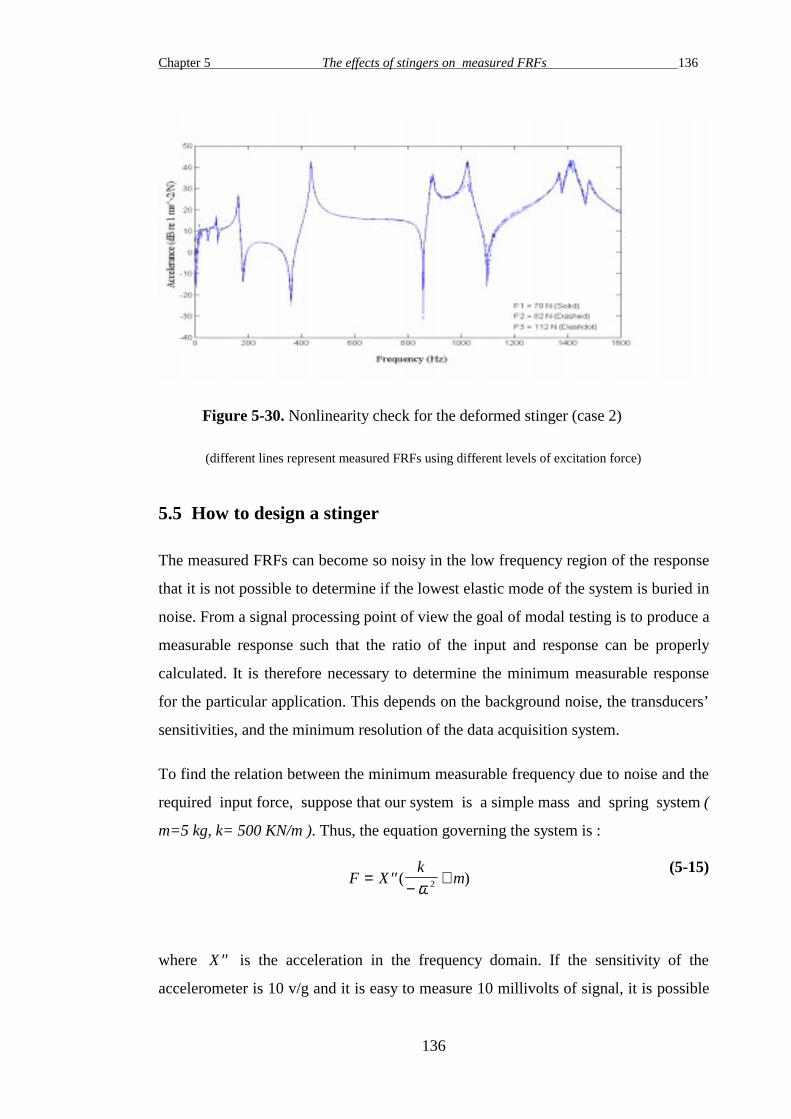
Chapter 5 The effects of stingers on measured FRFs 136
136
Figure 5-30. Nonlinearity check for the deformed stinger (case 2)
(different lines represent measured FRFs using different levels of excitation force)
5.5 How to design a stinger
The measured FRFs can become so noisy in the low frequency region of the response
that it is not possible to determine if the lowest elastic mode of the system is buried in
noise. From a signal processing point of view the goal of modal testing is to produce a
measurable response such that the ratio of the input and response can be properly
calculated. It is therefore necessary to determine the minimum measurable response
for the particular application. This depends on the background noise, the transducers’
sensitivities, and the minimum resolution of the data acquisition system.
To find the relation between the minimum measurable frequency due to noise and the
required input force, suppose that our system is a simple mass and spring system (
m=5 kg, k= 500 KN/m ). Thus, the equation governing the system is :
F Xk
m= ′′−
+( )ω 2
(5-15)
where ′′X is the acceleration in the frequency domain. If the sensitivity of the
accelerometer is 10 v/g and it is easy to measure 10 millivolts of signal, it is possible

Chapter 5 The effects of stingers on measured FRFs 137
137
to measure a response of 0.01g. In order to determine how much excitation force is
necessary, the minimum frequency of interest should be known. For example, if the
minimum frequency is 10 Hz then the required force is :
f = × ×− × ×
+ =( . ) ( . ) (( )
) .0 01 9 8500000
2 105 11922π N
If this same test is required to provide reliable data down to 2 Hz, then 309.85 N is
needed. For 1 Hz, then 1240.7 N is needed. Conversely, it is the reason that FRFs get
more and more noisy as the frequency diminish. Although this discussion holds for
sinusoidal excitation, practically, it holds for other excitation method as well.
It can be concluded that reliable FRF data in some part of the low frequency range
will be unobtainable. The effect of noise depends on the dynamic behaviour of the
structure which is under investigation by the modal test, the level of the background
noise and many other parameters. Therefore, there is no straightforward formula to
relate the input force and the level of the noise. However, a more powerful shaker will
decrease the effect of noise in the low frequency range.
Once the input force and the size of the shaker are chosen the following steps should
be followed to design the stinger:
Step 1- Calculate the minimum allowable diameter of the stinger. If the maximum
input force is P , and the material endurance stress of stinger is σ s , then :
σπ
ss
ssP
AA
d= =;
2
4
(5-16)
The minimum allowable diameter of the stinger is thus:
dP
smin =
4
πσ
(5-17)
The diameter of the stinger can be chosen to be greater than the minimum allowable
diameter ( dmin ). However, a thinner stinger is more flexible and has less effect on the
measured FRFs.

Chapter 5 The effects of stingers on measured FRFs 138
138
Step 2- Calculate the maximum allowable length of the stinger from Euler formula to
avoid the buckling of the stinger:
lE I
PI
ds ss
smax ;= =
264
2 4π π (5-18)
The length of the stinger cannot be more than lmax . However lmax is not the optimum
length of the stinger.
The most important part of designing a stinger is to choose the optimum length. If the
minimum and maximum desirable frequencies ( fmin and fmax ) are known, the
optimum length of the stinger should be chosen in such a way that the last
antiresonance in the low frequency range of the stinger is lower than fmin and the first
elastic antiresonance of the stinger is higher than fmax . This can be done by trial- and-
error of different lengths in the theoretical model of the stinger which was presented
in section 5.3.1.
Step 3- For a particular length of stinger, compute the antiresonance in the low
frequency region, as was discussed in section 5.3.3. For this computation the
parameters of the shaker and those of the structure are needed. It is important to add
the mass of the force transducer and that of the mounting hardware to the mass of the
structure. Moreover, it is necessary to add an additional length to the length of the
stinger to compensate for the length of the mounting hardware and that of the force
transducer. Based on the experience gained in section 5.4, this additional length is
2~3 mm.
Step 4- Calculate the first elastic antiresonance for the stinger of a particular length, as
was discussed in section 5.3.4. Table 5.2 shows some of these antiresonances for
different lengths and diameters of the steel stingers.
Step 5- Calculate the first antiresonance of the stinger in the axial direction using the
ANSYS model as was presented in section 5.3.8. If the first antiresonance of the
stinger in the axial direction is lower than that of the stinger in the bending direction
then the antiresonance in the axial direction should be more than fmax .

Chapter 5 The effects of stingers on measured FRFs 139
139
Step 6- After trying different lengths for the stinger, the optimum length can be
chosen so that the antiresonances of the stinger are not in the frequency range of fmin
to fmax .
Step 7- Determine a maximum allowable deflection of the stinger. The experimental
results of section 5.4 showed that the deformation of the stinger can bias the results
unacceptably. Based on the experience gained in section 5.4, it is recommended that
the deformation of the stinger should be restricted so that the change in the first
antiresonance of the stinger is less than 5 Hz. The procedure to calculate the change in
the first antiresonance of the stinger due to its misalignment was explained in section
5.3.6.
5.6 How to check the effects of a stinger on the measured FRFs
In the previous section we presented a procedure to design a stinger for the test so that
its effect on the measured FRFs become minimum. However, it is necessary to check
the effects of the stinger on the measurements for assessing the quality of the
measurement.
In the design of a stinger the main effort is to avoid the stinger’s antiresonances. If the
length of the stinger is changed slightly, its antiresonances (bending or axial) will
shift slightly in the frequency range. As a result, the effects of the antiresonances of
the stinger on the measured FRF will shift slightly and this is a sign of error. We
present this fact by a numerical example:
A steel beam was tested in a simulated shaker test using two different stingers (Figure
5-32 ). The parameters of the simulated test were:
Beam : Dimension : 0 02 0 006 0 44. . .× × m , Material: Steel.
Shaker : Mass : 10.5 kg, Rotary moment of inertia : 0.03 kg m. 2 , Suspension: ksh =
5400 N/m, krsh = 0 N-m/rad.
Stinger 1 : Diameter : 2 mm , Length : 0.075 m, Material : Steel.

Chapter 5 The effects of stingers on measured FRFs 140
140
Stinger 2 : Diameter: 2 mm, Length: 0.079 m, Material : Steel.
Measurement Set up : Excitation : at point 3, Response: at point 7.
Frequency range : 200-2000 Hz
Figure 5-33 shows that the location of the first elastic antiresonance of stinger 1 is at
1645 Hz and that of stinger 2 is at 1480 Hz. Figure 5-34 shows the effects of stingers1
and 2 on the measured FRF. This figure shows that by replacing stinger 2 with stinger
1, the effect of the latter stinger shifts slightly to the lower frequencies while the other
parts of the measured FRF remains unchanged. This suggests that by a slight change
in the length of the stinger, its effect on the measured FRF can be revealed.
Consequently, using this method the effect of a designed stinger on the measured FRF
can be checked.
Figure 5-31. Model used for the Simulated shaker test

Chapter 5 The effects of stingers on measured FRFs 141
141
Figure 5-32. Antiresonances of stingers 1 and 2
Figure 5-33. The effects of stingers 1 and 2 on the measured FRF

Chapter 5 The effects of stingers on measured FRFs 142
142
5.7 Design of a stinger in an actual test
A steel beam with a mass of 0.412 kg is to be experimentally tested for its dynamic
characteristics. The beam is to be suspended vertically with an elastic cord with the
stiffness of 410 N/m. A 80 N electromagnetic shaker is chosen to excite the structure.
The mass of the shaker is 10.5 kg (the mass of the coil is 0.21 kg) and its moment of
inertia is 0.03 Kg m. 2 . The shaker was suspended by a spring with the stiffness of
5400 N/m. The mass of the force transducer and that of the mounting hardware is
0.025 kg. The required frequency range of the measurement was 80 to 1250 Hz.
In order to find the optimum stinger for this test the procedure is:
The minimum diameter is calculated from equation (5-17) as:
46min 105.5
10345
804 −×=××
×=π
d m
In which σ s = ×345 106 N/m is the material endurance stress of the steel. The
diameter of the stinger can be chosen to be 1.5 mm. It should be mentioned that the
diameter of the stinger can be chosen to be greater than the minimum allowable
diameter ( dmin ). However, a thinner stinger is more flexible and has less effect on the
measured FRFs.
The maximum allowable length of the stinger can be calculated from equation (5-18)
as:
086.08064
)105.1(101212 4392
max =×
×××××=−ππ
l m
Calculations show that the last antiresonance in the low frequency range for a stinger
with the diameter of 1.5 mm and length of 25 mm is at 44.5 Hz and its first elastic
bending antiresonance is at 11080 Hz. The first axial anti resonance of this stinger is
at 4239 Hz. Therefore this stinger is suitable for measuring the FRFs of the beam in
the frequency range of 80 to 1250 Hz.

Chapter 5 The effects of stingers on measured FRFs 143
143
Calculations show that for a stinger with the diameter of 1.5 mm and length of 25
mm, when we have 2.1 mm misalignment between two ends of the stinger (Figure 5-
31) , the first elastic anti resonance of the stinger (in the axial direction) moves to
4234 Hz (5 Hz difference). As a result the misalignment between two sides of the
stinger should not exceed 2.1 mm.
Figure 5-34. Misalignment of the stinger
Figure 5.35 shows the result of the measurement of the beam in the actual test using
the stinger designed above with the following parameters:
Stinger 1 : Diameter : 1.5 mm , Length : 25 mm, Material : Steel.
In order to check the performance of stinger 1 another measurement was conducted
using another stinger with the same diameter but slightly different length. The
parameters of this stinger were:
Stinger 2 : Diameter : 1.5 mm , Length : 27 mm, Material : Steel.
Figure 5.35 shows the result of the measurement using stinger 2 which is drawn
together with the measured FRF using stinger 1. There is no considerable difference
between two measured FRFs. Therefore it can be concluded that stinger 1 (or stinger
2) is suitable for this test.
Figure 5-36 shows the result of the measurement of the beam in the actual test using
an unsuitable stinger. The parameters of this stinger are:
Stinger 3 : Diameter : 1.5 mm , Length : 82 mm, Material : Steel.

Chapter 5 The effects of stingers on measured FRFs 144
144
Another stinger with the same diameter but slightly different lengths was used to
reveal the effect of stinger 3 on the measured FRF (see Figure 5.36). The parameters
of this stinger are:
Stinger 4 : Diameter : 1.5 mm , Length : 85 mm, Material : Steel.
A comparison between two measured FRFs (using stingers 3 and 4) in Figure 5-36
shows that stinger 3 has affected the measured FRF at 1080 Hz and stinger 2 has shift
this effect to 1000 Hz. There is no discernible difference between two measured FRFs
at all the other frequencies. For comparison purposes the measured FRF using stinger
1 is shown in Figure 5-36. It can be concluded that stinger 3 is not suitable for the
measurement of the beam in the frequency range of 80-1250 Hz. Moreover, the result
of this test show that the method for assessing the performance of a stinger can show
the effects of an unsuitable stinger on the measured FRFs.
Figure 5-35. Checking of the performance of the designed stinger

Chapter 5 The effects of stingers on measured FRFs 145
145
Figure 5-36. Revealing of the effects of an unsuitable stinger on the measured FRF
5.8 Conclusions
• It was proven that the maximum error of the measured FRFs are due to the
antiresonances of the rotational driving point receptance of the tip of the stinger.
• In this chapter a new model was presented for the shaker-stinger-structure system.
This model allowed us to assess the effect of the misalignment of the stinger on its
performance.
• It was shown that when there is a misalignment between two ends of the stinger,
the antiresonances of the stinger shift to the lower frequencies and the measured
FRFs are biased. Therefore, a maximum allowable deformation of the stinger was
introduced based on the changes in the first elastic antiresonance of the stinger.

Chapter 5 The effects of stingers on measured FRFs 146
146
• The presented model was used for the calculations of the antiresonances of the
shaker-stinger-structure system which was successfully validated by the
experimental results of a free-free beam.
• Based on this study a design procedure was introduced which was followed by an
example.
• It was shown that the effects of the stinger on the measured FRF can be checked
by repeating the test with another stinger with the same diameter but slightly
different length.

Chapter 6 Correction of mechanical effects in more than one DOF 147
147
Chapter 6
Correction of mechanical effects in
more than one DOF
Reminder of Nomenclature
αij* measured receptance of a modified structure
n number of modification DOFs
nc number of different configurations
r number of unknowns
( )pii′α receptance of the attached mechanical element
at DOF i for pth configuration
[ ]′αii matrix of the receptances of attached mechanical
elements for different configurations
6.1 Introduction
The basic theory for the correction of mass-loading effects of a transducer in one DOF
was presented in chapter 3. In chapter 4 a similar method was developed for the
correction of the effects of a suspension spring on the test structure. However, the test
structure may be affected by mechanical devices in more than one DOF. By
mechanical devices we mean suspension springs, transducers and stingers or any other
mechanical elements which are used to conduct the modal test. In practice, there are
some cases that it is advantageous for us to cancel the effect of the mechanical
devices in more than one DOF (see chapters 8 and 9). Therefore, it is imperative to
generalise the correction method mathematically before dealing with more
complicated practical cases.
In this chapter a general solution for the correction of the effects of mechanical
devices on measured FRFs by modifying the test structure at its boundaries will be

Chapter 6 Correction of mechanical effects in more than one DOF 148
148
presented. It is shown that the FRFs can be corrected if the measurement is repeated
in a number of different configuration; each configuration consisting of the system
with one or more of its boundary conditions changed. It is also shown that the driving
point FRFs related to the degrees of freedom of the attachment of mechanical devices
can be computed without actually having to measure them. One of the applications of
these correction methods is in chapter 9 where the test structure is modified in two
DOFs by the mass and rotational inertia of an attached object in order to generate the
rotational FRFs.
6.2 Theory
6.2.1 Modification of the test structure in more than one DOF
Appendix A of this thesis investigates the general case of the changes in measured
FRFs due to the attachment of mechanical devices to the test structure. As shown at
this appendix, for the general case, when the test structure is modified in n DOFs, the
relation between the measured FRF and the exact FRFs is :
α
α α α αα α α α αα α α α α
α α α α αα α α α
α α α α
α α α α
lk
lk l l
k n
k n
nk n n nn nn
n
n
n n nn nn
*
ln
=
⋅ ⋅+ ′ ⋅ ⋅
+ ′ ⋅ ⋅⋅ ⋅ ⋅ ⋅ ⋅ ⋅⋅ ⋅ ⋅ ⋅ ⋅ ⋅
⋅ ⋅ + ′+ ′ ⋅ ⋅
+ ′ ⋅ ⋅⋅ ⋅ ⋅ ⋅ ⋅⋅ ⋅ ⋅ ⋅ ⋅
⋅ ⋅ + ′
1 2
1 11 11 12 1
2 21 22 22 2
1 2
11 11 12 1
21 22 22 2
1 2
(6-1)
Equation (6-1) can be rewritten as :
b xx a x a x a
x a x a x a arr r
r r r r r
= −+ + ⋅ ⋅ ⋅ +
+ + ⋅ ⋅ ⋅ + +++ + +
2 11 1 2 2
1 1 2 2 2 1
(6-2)

Chapter 6 Correction of mechanical effects in more than one DOF 149
149
where :
b lk= α * (6-3)
and a1, a2 , . . . , ar+1 are the multiplications of ′α ii ’s which are given in Table 6-1. In
the first row it is shown that a1 1= . In the second row it is shown that a2 11= ′α ,
a3 33= ′α , . . . , an nn+ = ′2 α . In the third row it is shown that an+ = ′ ′3 11 22α α ,
an+ = ′ ′4 11 33α α and so on until the last row that ar nn+ = ′ ′ ′ ⋅ ⋅ ⋅ ′1 11 22 33α α α α . The total
number of ai ’s is r n= −2 1.
Table 6-1. Parameters of equation (6-2)
ai considerations number of ai ’s
a1 1 1
a2 ,… ′α ii i n= 1 2, ,... , n
an+2 ,. ′ ′α αii jj i j n, , , ... ,= 1 2 and i j≠ n n× −( )1 2
. ′ ′ ′α α αii jj kk i j k n, , , , ... ,= 1 2 and
i j k≠ ≠
n n n× − × − ×( ) ( )1 2 3 2
.
.
.
.
.
.
. .
. .
. .
.
.
.
ar+1 ′ ′ ′ ⋅ ⋅ ⋅ ′α α α α11 22 33 nn 1
Total number of ai ’s ( )r + 1 2n

Chapter 6 Correction of mechanical effects in more than one DOF 150
150
x si ’ are unknowns and are a combination of α ij ’s, x r2 1+ is :
x r lk2 1+ = α (6-4)
xr+1, xr+2 , . . . , x r2 are a combinations of α11, α22 , . . . , αnn . Especially we have :
x
x
x
r n
r n
r nn
2 1 11
2 2 22
2
− +
− +
==
=
αα
α
.
.
.
(6-5)
x1, x2 , . . . , xr are a combination of α11, α22 , . . . , αnn ,α1k , α2k , . . . , αnk and
α l1, α l2 , . . . , α ln .
6.2.2 Correction of the FRFs
Correction of the measured FRFs for the case where a structure is modified in more
than one DOF can essentially be accomplished in two main ways :
1. step by step correction : in this approach in each step the effect of one of the
mechanical elements corresponding to one DOF is corrected, while the others are
constant. An application of this approach for the case of a structure which is
modified by two springs in two different DOFs was given in section 4.2.3.( This
approach will be used for the generation of rotational FRFs in chapter 9)
2. direct correction : in this approach the structure is tested in a number of different
configurations; each configuration consists of the structure with one or more of its
boundary conditions changed. Using the data of these tests the effects of the
mechanical devices on measured FRFs can be corrected by numerical procedures.
The direct correction approach is the main concern of this chapter.
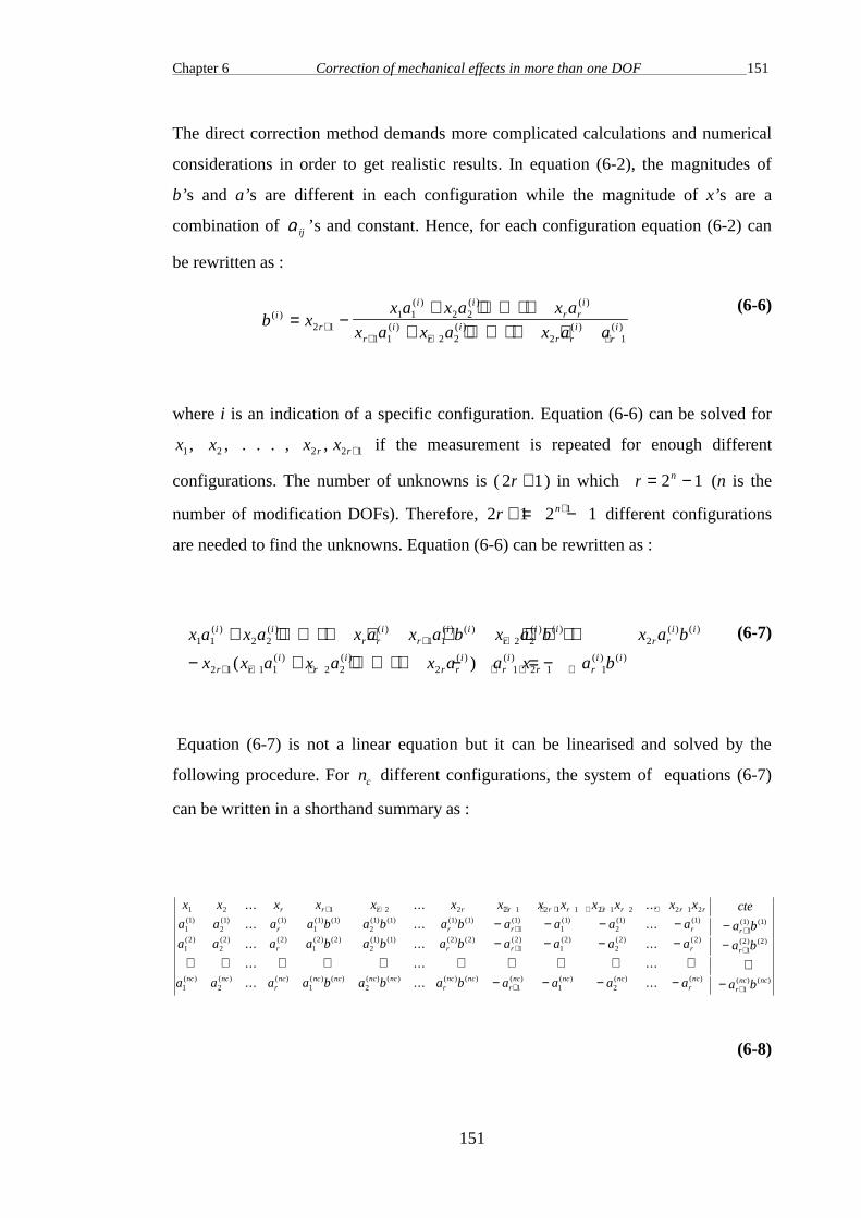
Chapter 6 Correction of mechanical effects in more than one DOF 151
151
The direct correction method demands more complicated calculations and numerical
considerations in order to get realistic results. In equation (6-2), the magnitudes of
b’s and a’s are different in each configuration while the magnitude of x’s are a
combination of α ij ’s and constant. Hence, for each configuration equation (6-2) can
be rewritten as :
b xx a x a x a
x a x a x a ai
r
i ir r
i
ri
ri
r ri
ri
( )( ) ( ) ( )
( ) ( ) ( ) ( )= −+ + ⋅ ⋅ ⋅ +
+ + ⋅ ⋅ ⋅ + +++ + +
2 11 1 2 2
1 1 2 2 2 1
(6-6)
where i is an indication of a specific configuration. Equation (6-6) can be solved for
x1, x2 , . . . , x r2 , x r2 1+ if the measurement is repeated for enough different
configurations. The number of unknowns is (2 1r + ) in which r n= −2 1 (n is the
number of modification DOFs). Therefore, 2 1 2 11r n+ = −+ different configurations
are needed to find the unknowns. Equation (6-6) can be rewritten as :
x a x a x a x a b x a b x a b
x x a x a x a a x a b
i ir r
ir
i ir
i ir r
i i
r ri
ri
r ri
ri
r ri i
1 1 2 2 1 1 2 2 2
2 1 1 1 2 2 2 1 2 1 1
( ) ( ) ( ) ( ) ( ) ( ) ( ) ( ) ( )
( ) ( ) ( ) ( ) ( ) ( )( )
+ + ⋅ ⋅ ⋅ + + + + ⋅ ⋅ ⋅ +
− + + ⋅ ⋅ ⋅ + − = −+ +
+ + + + + +
(6-7)
Equation (6-7) is not a linear equation but it can be linearised and solved by the
following procedure. For nc different configurations, the system of equations (6-7)
can be written in a shorthand summary as :
x x x x x x x x x x x x x
a a a a b a b a b a a a a
a a a a
r r r r r r r r r r r
r r r r
r
1 2 1 2 2 2 1 2 1 1 2 1 2 2 1 2
11
21 1
11 1
21 1 1 1
11
11
21 1
12
22 2
... ... ...
... ... ...
...
( ) ( ) ( ) ( ) ( ) ( ) ( ) ( ) ( ) ( ) ( ) ( ) ( )
( ) ( ) ( )
+ + + + + + + +
+− − − −
12 2
21 1 2 2
12
12
22 2
1 2 1 2 1 1 2
( ) ( ) ( ) ( ) ( ) ( ) ( ) ( ) ( ) ( )
( ) ( ) ( ) ( ) ( ) ( ) ( ) ( ) ( ) ( ) ( ) ( ) (
... ...
... ... ...
... ... ...
b a b a b a a a a
a a a a b a b a b a a a a
r r r
nc ncr
nc nc nc nc ncr
nc ncr
nc nc ncr
− − − −⋅ ⋅ ⋅ ⋅ ⋅ ⋅ ⋅ ⋅ ⋅ ⋅
− − − −
+
+nc
r
r
rnc nc
cte
a b
a b
a b)
( ) ( )
( ) ( )
( ) ( )
−−
⋅−
+
+
+
11 1
12 2
1
(6-8)

Chapter 6 Correction of mechanical effects in more than one DOF 152
152
To find the solution for the system of equations (6-8), a procedure like the Gauss
elimination method can be used [98]. If the elements of the second row of equations
(6-8) are multiplied by a12( ) and the elements of the third row by a1
1( ) and the
elements of the third row are subtracted from the elements of the second row then x1
and x xr r2 1 1+ + will be eliminated from the resulted equations. This procedure can be
repeated for the second row and other rows of equation (6-8). The resulting equation
is :
x x x x x x x
a a a a a a a a a a b b
a a a a a a a a
r r r r r r
r r
r r
2 1 2 2 1 2 1 2
22
11
21
12 2
11 1
12
12
11 2 1
23
11
21
13 3
11 1
13
... ... ...
... ( ) ... ...
...
( ) ( ) ( ) ( ) ( ) ( ) ( ) ( ) ( ) ( ) ( ) ( )
( ) ( ) ( ) ( ) ( ) ( ) ( ) (
+ + + +
− − − ⋅ ⋅ ⋅− − ) ( ) ( ) ( ) ( )
( ) ( ) ( ) ( ) ( ) ( ) ( ) ( ) ( ) ( ) ( ) ( )
( ) ... ...
... ... ...
... ( ) ... ...
a a b b
a a a a a a a a a a b b
cte
nc ncr
ncr
nc nc nc nc
13
11 3 1
2 11
21
1 11
1 1 11 1
− ⋅ ⋅ ⋅⋅ ⋅ ⋅ ⋅ ⋅ ⋅− − − ⋅ ⋅ ⋅
⋅⋅⋅⋅
(6-9)
If the same procedure is followed to eliminate x2 and x xr r2 1 2+ + from equation (6-9)
and the procedure is followed to eliminate x1, x2 , . . . , xr all nonlinear elements will
be eliminated. The final resulting equation is :
x x x x
q q q q
q q q q
q q q q
cte
p
p
p
r r r r
r r
r r
nc r nc r nc r r nc r r nc r
+ + +
+
+
− − − − + −
⋅ ⋅ ⋅ ⋅ ⋅ ⋅
1 2 2 2 1
11 12 1 1 1
21 22 2 2 1
1 2 1
1
2
...
...
...
...
( )
( )
( ) ( ) ( ) ( )( ) ( )
(6-10)
Equations (6-10) are a series of linear equations of the form :
q q q q
q q q q
q q q q
x
x
x
p
p
p
r r
r r
nc r nc r nc r r nc r r
r
r
r nc r
11 12 1 1 1
21 22 2 2 1
1 2 1
1
2
2 1
1
2
...
...
...
...
.
( )
( )
( ) ( ) ( ) ( )( ) ( )
+
+
− − − − +
+
+
+ −
⋅ ⋅ ⋅ ⋅
= ⋅
(6-11)
This equation can be summarised as :

Chapter 6 Correction of mechanical effects in more than one DOF 153
153
[ ]{ } { }q x prr+
+ =12 1 (6-12)
in which:
{ }x
x
x
x
r
r
r
r
r
++
+
+
+
=
1
2 1
1
2
2 1
. ( 6-13)
and the solution is :
{ } [ ] { }x q prr+
+ +=1
2 1 (6-14)
where [ ]q+
is the pseudo-inverse of [ ]q . To find x1, x2 , . . . , xr equation (6-14) can
be rewritten as :
x a x a x a x b x a x a x a ai ir r
ir
ir
ir
ir r
iri
1 1 2 2 2 1 1 1 2 2 2 1( ) ( ) ( ) ( ) ( ) ( ) ( ) ( )( )( )+ + ⋅ ⋅ ⋅ + = − + + ⋅ ⋅ ⋅ + ++ + + +
(6-15)
Knowing xr+1, xr+2 , . . . , x r2 from (6-14), the right hand side of equation (6-15) is
known. So equations (6-8) can be rearrenged as :
x x x
g g g
g g g
g g g
cte
v
v
v
r
r
r
nc nc ncr nc
1 2
11 12 1
21 22 2
1 2
1
2
. .
. .
. .
. .
⋅ ⋅ ⋅ ⋅ ⋅ ⋅(6-16)
or :
[ ]{ } { }g x vr1 = (6-17)
and the solution is :
Chapter 6 Correction of mechanical effects in more than one DOF 154
154
{ } [ ] { }x g vr1 =
+ (6-18)
in which [ ]g+
is the pseudo-inverse of [ ]g . The Pseudo-inverse has been used in
equations (6-18) and (6-14) to show that the number of equations can be more than
the number of unknowns. In this case [ ]g or [ ]q is not square and the pseudo-inverse
should be used to find the unknowns. When the data are noisy, increasing the number
of equations and using the pseudo-inverse will average the solution and decrease the
effect of noise. It should be emphasised that the condition to solve the equations (6-
11) is :
nc n≥ −+2 11 (6-19)
By solving equations (6-11) and finding x1, x2 , . . . , x r2 , x r2 1+ and from equation (6-
4), α lk , the exact receptance, can be found. Moreover, from equations (6-5) the
correct value of α11 , α22 , . . . and αnn can be obtained.
The above procedure is a direct method for cancellation of the effects of mechanical
devices in more than one DOF. Equation (6-19) show that when the test structure is
modified in two DOFs, at least 7 different tests with different configurations are
needed to cancel the mechanical effects. In the next section the practical aspects of
this method will be studied.
6.3 Demonstration and verification of the method
6.3.1 Programming considerations
In the last section it was shown how a measured FRF of a structure which is modified
in n DOFs can be corrected using direct approach. To program the method suggested
in the last section, the following steps have to be considered:

Chapter 6 Correction of mechanical effects in more than one DOF 155
155
1- arrange the receptances of the attached mechanical devices in each DOF in a
matrix in which each row is for one configuration:
[ ]′ =
′ ′ ⋅ ⋅ ⋅ ′′ ′ ⋅ ⋅ ⋅ ′
⋅ ⋅ ⋅ ⋅ ⋅ ⋅⋅ ⋅ ⋅ ⋅ ⋅ ⋅⋅ ⋅ ⋅ ⋅ ⋅ ⋅
′ ′ ⋅ ⋅ ⋅ ′
α
α α αα α α
α α α
( ) ( ) ( )
( ) ( ) ( )
( ) ( ) ( )
111
122
1
211
222
2
11 22
nn
nn
nc nc ncnn
(6-20)
2- arrange the measured FRFs in a column matrix { }b as :
{ }b
lk
lk
nclk
=
( ) *
( ) *
( ) *
.
.
1
2
αα
α
(6-21)
3- To calculate the a’s as is shown in table 6-1, all the multiplications of the
elements of matrix [ ]′α in each row are needed. Table 6-2 shows a typical
example of the procedure which is used to calculate the a’s from one row of
matrix [ ]′α for the case where n=5. Each column can be built from the last
column. In the first step (k=1), a1 to a5 are equal to ′α11 to ′α55 . In the second step
(k=2), a6 is made from the multiplication of a2 by a1 . Multiplying of a3 by
a1 and a2 , yields a7 and a8 respectively. a4 is multiplied by a1 , a2 and a3 which
yields a9 , a10 and a11 and so on. In the same way all the multiplications of ′α ii’s
are made as is shown in Table 6-2.

Chapter 6 Correction of mechanical effects in more than one DOF 156
156
Table 6-2. Programming of the multiplication of a set of ′α ii’s
No. k=1 k=2 k=3 k=4 k=5
1 a1 11= ′α 1 a a a6 1 2= 1 a a a16 6 3= 1 a a a26 16 4= 1 a a a31 26 5=
2 a2 22= ′α a a a7 1 3= a a a17 6 4= a a a27 16 5=
3 a3 33= ′α 2 a a a8 2 3= a a a18 7 4= a a a28 17 5=
4 a4 44= ′α a a a9 1 4= 3 a a a19 8 4= a a a29 18 5=
5 5 a5 55= ′α a a a10 2 4= a a a20 6 5= 4 a a a30 19 5=
6 3 a a a11 3 4= a a a21 7 5=
7 a a a12 1 5= a a a22 8 5=
8 a a a13 2 5= a a a23 9 5=
9 a a a14 3 5= a a a24 10 5=
10 4 a a a15 4 5= 6 a a a25 11 5=
4. make matrix [ ]a as:
[ ]a
a a a
a a a
a a a
r
r
nc nc ncr
=
⋅ ⋅ ⋅⋅ ⋅ ⋅
⋅ ⋅ ⋅ ⋅ ⋅ ⋅⋅ ⋅ ⋅ ⋅ ⋅ ⋅⋅ ⋅ ⋅ ⋅ ⋅ ⋅
⋅ ⋅ ⋅
+
+
+
1
1
1
1
1
1
11
12
11
21
22
21
1 2 1
( ) ( ) ( )
( ) ( ) ( )
( ) ( ) ( )
(6-22)
where a’s were made in the last stage.
5. multiply the last column of matrix [ ]a by -1.

Chapter 6 Correction of mechanical effects in more than one DOF 157
157
6. multiply each row of [ ]a by the element of [ ]b in the same row and add the result
to matrix [ ]a .
7. do the elimination procedure explained in section 6.2.2 and find the solution.
6.3.2 Numerical case study
To prove the validity of the method, a beam was considered in a simulated test
(Figure 6-1). The beam was modified by the addition of an object which has both
mass and rotational inertia properties. The object was attached to the structure at
DOFs 3 and 4. The beam was excited at DOF 7 and the response is measured at DOF
9.
Figure 6-1. A simulated test on a beam
( TDOFs = Translational Degrees of Freedom , RDOFs = Rotational Degrees of Freedom )
The theoretical model of the beam was built using the concept of coupling the free-
free beam elements as was explained in chapter 3 .
The attached object modifies the beam by changing the dynamic stiffness matrix of
the beam, at DOFs 3 and 4 as :
D D mmd ( , ) ( , )3 3 3 3 2= − ω (6-23)
and:
D D Imdb( , ) ( , )4 4 4 4 2= − ω (6-24)
The specifications of the beam and those of the attached object are given in Table 6-3.

Chapter 6 Correction of mechanical effects in more than one DOF 158
158
Table 6-3. Parameters of the theoretical beam
Length of t beam 0.44 ( m )
Height of beam 0.02 ( m )
Thickness of beam 0.006 ( m )
Number of elements in beam 10
Mass of density 7800 ( kg m/ 3 )
Mass 0.412 (kg)
Modulus of elasticity 2e11 ( N m/ 2 )
Mass of the attached object 0.05 kg
Moment of inertia of the attached object 1 10 5× − ( kg m. 2)
Once the main effects of the mass and rotational inertia properties of the attached
object were included in the model of the beam a simulated experiment was performed
in order to determine the effects of the attached object on the measured FRFs of the
beam. Figure 6-2 shows the comparison of the affected FRF and the exact FRF.
Figure 6-2. The comparison of A79 and the affected A79 of the beam

Chapter 6 Correction of mechanical effects in more than one DOF 159
159
According to equation (16) of Appendix A, the receptance of the modified beam is
equal to:
α αα α α α α α
α α α α α α97 9747 33 33 43 37 94
44 44 33 33 34 43
* [ ( ) ]
( )( )= −
+ ′ −+ ′ + ′ −
+− + ′
+ ′ + ′ −[ ( )]
( )( )
α α α α α αα α α α α α
47 34 37 44 44 93
44 44 33 33 34 43
(6-25)
From equation (6-2) for the case of n=2 and r is equal to 2 1 3n − = we have :
b xx a x a x a
x a x a x a a= −
+ ++ + +7
1 1 2 2 3 3
4 1 5 2 6 3 4
(6-26)
in which:
x
x
x
x
x
x
x
1 47 33 43 37 94 47 34 37 44 93
2 47 94
3 37 93
4 44 33 34 43
5 44
6 33
7 97
= − + −=
= −= −
===
( ). ( ).α α α α α α α α α αα αα α
α α α αααα
(6-27)
and:
a
a
a
a
1
2 33
3 44
4 33 44
1== ′= ′
= ′ ′
αα
α α
, b = α97* (6-28)
The beam has been modified in 2 DOFs, therefore, according to equation (6-19), at
least seven different configurations (mass and rotational inertia of the attached object)
are needed to correct the measured FRFs based on the method presented in this

Chapter 6 Correction of mechanical effects in more than one DOF 160
160
chapter. Equation (6-27) gives the unknown parameters and equation (6-28) gives the
known parameters.
Table 6-4 shows different parameters of the attached object for 7 different simulated
measurements. Two different sets were considered. Figures 6-3 to 6-5 show the
results of applying the correction method using set 1 of Table 6-4. The interesting
point of this correction method is that in the simulated measurement the rotational
point FRF, α44 , is obtained while the translational force and responses were actually
measured ( Generation of rotational FRFs using correction methods is the subject of
chapter 9).
Figures 6-6 to 6-8 show the results of applying the correction method using set 2 of
Table 6-4. While the computed transfer FRF matches the exact FRF (Figure 6-6), the
computed point FRFs are meaningless (Figures 6-7 and 6-8). This problem arises
from the rank deficiency of matrix [g] in equation (6-18). The rank of the matrix
which is built based on the information of set 1 in Table 6-4 is 4 for all of the
frequency points while for the second set it is 3. Thus for set 2, matrix [g] is rank
deficient and the inverse of this matrix, for some elements, is meaningless.
Here the effect of noise has not been considered. However, in the presence of rank
deficiency, using noisy data makes the results more unreliable. The reason for this
rank deficiency is choosing of an improper set of objects which modify the test
structure. Matrix [ ]′α in equation (6-20), which is the matrix of the receptances of
the attached objects, is part of the matrix [g] for all of the frequencies. Therefore if the
matrix [ ]′α is rank deficient, matrix [g] will be rank deficient as well. The rank of
matrix [ ]′α for the first set of objects in Table 6-4 is 2 and its condition number is
17 103. × . For the second set, the rank of matrix [ ]′α is 1 and its condition number is
∞ . As a result, for the second set the results are expected to be unreliable.
Therefore the best way to cope with rank-deficiency is just by choosing a proper set
of configurations which creates a matrix of full rank [ ]′α in equation (6-20). This
means that the objects which modify the structure need to be selected to avoid
numerical difficulties. Fortunately, this design is not case dependent in the sense that

Chapter 6 Correction of mechanical effects in more than one DOF 161
161
the behaviour of the structure does not have any effect on these numerical problems.
For the special case that the test structure is modified in one DOF only (the subject of
chapters 3 and 4), matrix [ ]′α is:
[ ]′ =
′′
⋅⋅
′
α
αα
α
( )
( )
( )
111
211
11nc
(6-29)
in which nc ≥ 3. In this case the rank of the matrix is 1 and may not be made rank-
deficient by choosing an improper set of objects.
Table 6-4. Two series of data for the correction
Set 1 Set 2
m (kg) I ( Kg m. 2 ) m (kg) I ( Kg m. 2 )
1 0.05 1 10 5× − 0.05 1 10 5× −
2 0.06 11 10 5. × − 0.055 11 10 5. × −
3 0.025 7 10 6× − 0.045 9 10 6× −
4 0.033 7 5 10 6. × − 0.06 12 10 5. × −
5 0.1 15 10 5. × − 0.0425 85 10 6. × −
6 0.075 9 10 6× − 0.0575 115 10 5. × −
7 0.038 5 10 6× − 0.035 7 10 6× −
6.4 Discussion
The method developed in this chapter provide a mathematical basis for the correction
of the mechanical devices effects on the test structure in more than one DOF.
However, in practice, applications of these methods are limited. For example when

Chapter 6 Correction of mechanical effects in more than one DOF 162
162
the test structure is modified in two DOFs by a suspension spring and an
accelerometer, 7 different measurements with different configurations are needed to
obtain the exact FRF. If the test structure is modified in three DOFs, 15 different
measurements with different configurations are needed. In practice, conducting this
number of tests with different configurations is not cost efficient. Moreover, the
effects of noise and other errors pollute the results of the correction due to the large
number of the computation levels.
The application of the methods presented in this chapter is in chapter 9 where the test
structure is modified by the mass and rotational inertia of an attached object in two
DOFs in order to generate the rotational FRFs.
6.5 Conclusions
• In this chapter a general solution for the correction of the effects of mechanical
elements on the measured FRFs was presented.
• It was shown that if the measurement is repeated in a number of different
configurations, the exact FRFs are obtainable using two main approaches namely
the direct approach and the step-by-step approach. The direct approach was
developed in this chapter.
• It was shown that the driving point FRFs of the degree of the freedom of the
attachment of mechanical devices can be generated the correction method.
• In the direct approach, numerical errors can be avoided in the calculations due to
rank-deficiency of the matrices by selecting proper mechanical elements.

Chapter 6 Correction of mechanical effects in more than one DOF 163
163
Figure 6-3. Comparison of the Exact FRF,α79 ,and the computed FRF (set 1)
Figure 6-4. Comparison of the Exact FRF,α33 ,and the computed FRF (set 1)
Figure 6-5. Comparison of the Exact FRF,α44 ,and the computed FRF (set 1)

Chapter 6 Correction of mechanical effects in more than one DOF 164
164
Figure 6-6. Comparison of the Exact FRF,α79 ,and the computed FRF (set 2)
Figure 6-7. Comparison of the Exact FRF,α33 ,and the computed FRF (set 2)
Figure 6-8. Comparison of the Exact FRF,α44 ,and the computed FRF (set 2)

Chapter 7 The effect of nonlinearity on the correction methods of mechanical devices 165
165
Chapter 7
The effect of nonlinearity on the correction methods
of mechanical devices
7.1 Introduction
Most of the theory upon which modal testing is founded relies heavily on the
assumption that the test structure’s behaviour is linear. In practice, real structures are
seldom completely linear. In the correction methods presented in the previous
chapters, the main assumption was the linear behaviour of the test structure and those
of the attached elements. However, if the structure or the attached elements exhibits
nonlinear behaviour, the result of the correction is unreliable. In this chapter the effect
of nonlinearity on the correction methods which was presented in the previous
chapters will be investigated. Application of this study is in chapter 9 where the test
structure is modified by an object to generate rotational FRFs.

Chapter 7 The effect of nonlinearity on the correction methods of mechanical devices 166
166
7.2 The effect of nonlinearity of the test structure
Figure 7-1 indicates a structure which is modified at point l by a mass, m. According
to equation (3-12) in chapter 3, accelerance Alil( ) can be written with respect to the
original FRFs as :
AA
mAlil li
ll
( ) =+1
(7-1)
It was shown in chapter 3 that when the measurement is repeated with two different
masses, m1 and m2 , the correct values Ali and All can be computed from:
A
AA
m
Am
li
ll
lil
lil
=−
−
−1
1
1
1
1
2
1
( )
( )
(7-2)
If the measurement is repeated with another mass, m3 , then Ali can be computed
again as :
$( )
AA
m Ali
lil
ll
=−1 3
(7-3)
in which $Ali is the second computed FRF and All is computed from equation (7-2).
Figure 7-1. Correction of the FRFs for a nonlinear structure
If the assembly of the structure and the modification masses show any nonlinearity,
then the amount of Ali computed by equation (7-2) is different from $Ali computed by

Chapter 7 The effect of nonlinearity on the correction methods of mechanical devices 167
167
equation (7-3). In this case, the addition of mass m is a kind of passive excitation that
changes the effective force which excites the test structure. By attaching mass m to
the structure, as it acts like a passive force, the level of displacement at the point of
attachment can be restricted to a range of motion that produces linear response.
This conclusion applies to general cases where the structure is modified in more than
one DOF. If the assembly of the structure and/or the attached objects show any
nonlinearity, the results of the correction method is not the same for different sets of
data related to different configurations of the test structure.
7.2.1 Numerical example
To demonstrate the effect of the nonlinearity on the corrected FRFs, a simple model
of a mass and a hardening spring is considered (Figure 7-2).
Figure 7-2. One DOF nonlinear system
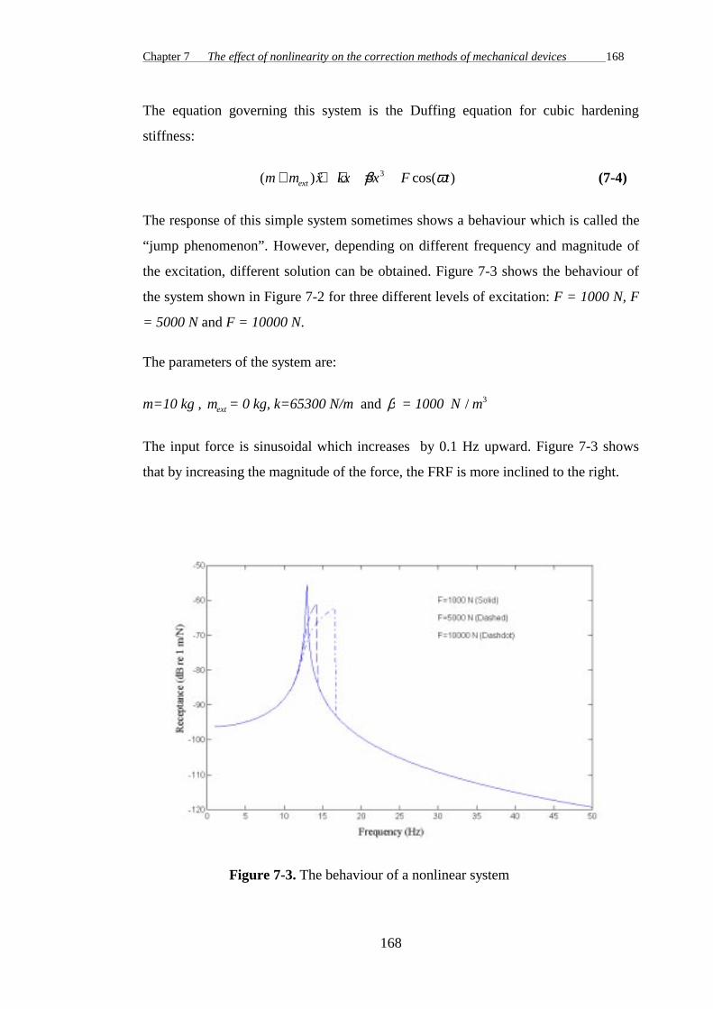
Chapter 7 The effect of nonlinearity on the correction methods of mechanical devices 168
168
The equation governing this system is the Duffing equation for cubic hardening
stiffness:
( )&& cos( )m m x kx x F text+ + + =β ω3 (7-4)
The response of this simple system sometimes shows a behaviour which is called the
“jump phenomenon”. However, depending on different frequency and magnitude of
the excitation, different solution can be obtained. Figure 7-3 shows the behaviour of
the system shown in Figure 7-2 for three different levels of excitation: F = 1000 N, F
= 5000 N and F = 10000 N.
The parameters of the system are:
m=10 kg , mext = 0 kg, k=65300 N/m and β = 1000 N m/ 3
The input force is sinusoidal which increases by 0.1 Hz upward. Figure 7-3 shows
that by increasing the magnitude of the force, the FRF is more inclined to the right.
Figure 7-3. The behaviour of a nonlinear system

Chapter 7 The effect of nonlinearity on the correction methods of mechanical devices 169
169
Figure 7-4 shows the result of the addition of an extra mass to the system shown in
Figure 7-2 while the level of the force is constant at 10000 N. If a mass of 5 Kg is
added to the system, the peak of the FRF shifts to the left and the system still shows
the jump phenomenon. By addition of 40 Kg extra mass to the system, the peak of the
FRF shifts even more to the left but the system shows little nonlinear behaviour.
Addition of the mass decreases the amplitude of the vibration and this linearises the
dynamic behaviour of the system.
Figure 7-4. Addition of the extra masses to the system while the level of the force is
constant (10000 N)
The correction process which was suggested in the previous chapters is based on the
linear behaviour of the structure. If the structure is nonlinear, the result of the
correction is different for different sets of data corresponding to different
configurations. Assuming the linear behaviour for the system shown in Figure 7-2, the
measured FRF can be corrected using the equation:

Chapter 7 The effect of nonlinearity on the correction methods of mechanical devices 170
170
αα
ω α1111
1
211
11=
+
( )
( )mext
(7-5)
The result of this correction is shown in Figure 7-5. Because of the nonlinearity, the
computed FRFs do not coincide with each other. For comparison purposes, the FRF
of the system when β = 0 in equation (7-4) is shown. In the case where the extra
mass is 40 Kg the computed FRF from equation (7-5) coincides with the linear FRF
in most of the frequency region. This coincidence proves that by addition of more
masses the structure shows more linear behaviour.
Figure 7-5. The result of the correction for the nonlinear structure
This study implies that the correction methods for nonlinear structures fail to provide
a unique solution for different sets of data.
7.3 The effect of nonlinearity of the attached objects
From the practical point of view, the elements which are attached to the test structure
may not show linear behaviour in the correction process. Therefore the correction

Chapter 7 The effect of nonlinearity on the correction methods of mechanical devices 171
171
process may fail to have a unique solution because of the nonlinear behaviour of
attached elements.
7.3.1 Numerical example
Figure 7-6 shows a one DOF system of mass and spring which is modified by a
nonlinear hardening spring. Two different nonlinear springs used for the correction of
the measured FRF. The parameters of the system and those of the nonlinear springs
are:
One DOF system: m = 10 kg , k = 65300 N/m;
Nonlinear spring 1: kext = 9700 N/m , βext = 1000 N m/ 3 ;
Nonlinear spring 2: kext = 24700 N/m , βext = 2000 N m/ 3 ;
Figure 7-6. Addition of a nonlinear spring
Figure 7-7 shows the receptance of the system when the magnitude of the force is
10000 N.

Chapter 7 The effect of nonlinearity on the correction methods of mechanical devices 172
172
Figure 7-7. The effect of a nonlinear spring on the system
If springs 1 and 2 are considered to be linear ( βext = 0 ), the effect of the additional
spring on the computed FRF can be removed by equation:
αα
α1111
1
1111
=−
( )
( )kext
(7-6)
The result of this correction is shown in Figure 7-8. The receptance of the original
linear system is shown for comparison. The FRFs do not coincide in some parts of the
frequency region. Therefore the results of the correction is not the same when the
attached elements do not show linear behaviour.

Chapter 7 The effect of nonlinearity on the correction methods of mechanical devices 173
173
Figure 7-8. Correction of an FRF affected by a nonlinear spring
7.4 The effect of other errors on the correction methods
In previous sections it was shown that in the presence of nonlinearity the results of the
correction methods for different sets of data are not the same. However, there are
other parameters which may cause the same effects on the correction methods. For
example, signal processing errors like leakage or the effect of the window functions
may cause the same problem. When a structure is modified by addition of mechanical
elements, in the presence of signal processing errors, the response signal of the
modified structure may not have the same results in the correction methods. One of
the most serious problems which may cause difficulty in the correction methods is the
relative phase shift between the force and acceleration signals. This problem was first
reported by McConnell in [99]. He showed that large measurement errors occur near
resonances in the mass cancellation process when there is a small relative phase shift
between the force and acceleration signals. The phase shift between the force and
acceleration signals may happen because of the mechanical and electrical effects in
each data channel, including amplifiers and anti-aliasing filters. In practice the phase

Chapter 7 The effect of nonlinearity on the correction methods of mechanical devices 174
174
shift between the force and acceleration signals can not be avoided, so any correction
method is subject to these large errors and must be used with caution.
7.5 Conclusions
• if the structure or the attached elements exhibits nonlinear behaviour, the results
of the correction methods are not the same using different sets of data
corresponding to different configurations.
• As most types of nonlinearity are amplitude-dependent, the attached mechanical
elements can be chosen so that the level of the motion of the structure is restricted
to a range of motion that produces linear response.
• There are other sources of systematic errors in modal testing which may cause the
same effects on the correction methods.

Chapter 8 Generation of the whole matrix of translational FRFs from measurements of one column
174
174
Chapter 8
Generation of the whole matrix of translational FRFs
from measurements of one column
8.1 Introduction
Measurement of the FRFs is a primary objective of modal testing in order to build a
mathematical model representing the dynamic behaviour of a structure. When the
number of DOFs is large, measuring the whole FRF matrix is difficult and sometimes
impossible. However, it is possible to compute the unmeasured FRFs from the
measurement and analysis of the FRFs in a single row (Response fixed)or column
(Force fixed) of the FRF matrix [5]. The unmeasured FRFs can, in principle, be
synthesised from the measured FRFs using the identified modal properties. However,
generating the unmeasured FRFs from the measured ones along a single row or
column is only theoretically possible when the frequency range covered extends from
zero to infinity. In practice, it is necessary to limit the frequency range of
measurement for obvious reasons. The remaining part, due to the out of range modes
- the residual - is not available and, as a result, estimating the unmeasured FRFs from
the measured ones is not accurate unless values for the relevant residual terms can be
estimated. In the past, some efforts have been made to relate the residual effects of
out-of-range modes between measured and unmeasured FRFs, but without much
success. At present, there is no known method to include the residual terms in the
calculation exactly.
The idea of evaluating the whole FRF matrix from measurement of some elements by
changing the boundary was suggested in [37]. As shown there, it is possible to
calculate some FRFs by modifying the structure at the points of interest at its
boundaries. New accelerometers were added to the points for each new set of
This work was published in IMAC 1998 [100].

Chapter 8 Generation of the whole matrix of translational FRFs from measurements of one column
175
175
Measurement. Thus, for an n DOF system, n accelerometers or dummy masses are
needed.
The challenge addressed in the present work is to develop a method for generating the
whole matrix of translational FRFs based on measurements using one accelerometer
and one dummy mass. The theory of the method is based on the direct substructuring
technique, Structural Modification Using experimental frequency Response Functions
(SMURF). Two different approaches are used to develop the governing equations of a
structure modified with two masses. Moreover, it has been shown that in noisy
environments, and when the masses of accelerometer and dummy mass are large, the
computation is relatively insensitive to noise.
8.2 Theory
In chapter 3, the modification of a structure by an added mass was studied. Figure 8-1
shows a structure which is modified with two different masses at points i and j .
Figure 8-1. Attachment of two masses
Two different approaches can be used to derive equations governing the modified
system, as discussed below:

Chapter 8 Generation of the whole matrix of translational FRFs from measurements of one column
176
176
8.2.1 Successive substitution
For the system shown in Figure 8-1, one can consider that mass mi is attached at
point i to the system composed of mass mj and structure C (Figure 8-2).
Figure 8-2. Addition of mass mi to structure C and mass mj
For this case, we have :
A AA A
mA
lki j
lkj ik
jli
j
iii
j
( , ) ( )( ) ( )
( )= −
+1 (8-1)
The accelerances of the modified structure Alkj( ) , Aik
j( ) , Alij( ) and Aii
j( ) can be written
in terms of the accelerances of the basic structure, C. we have :
A AA A
mA
lkj
lk
jk lj
jjj
( ) = −+
1 (8-2)
A AA A
mA
ikj
ik
jk ij
jjj
( ) = −+
1 (8-3)
A AA A
mA
lij
li
ji lj
jjj
( ) = −+
1 (8-4)

Chapter 8 Generation of the whole matrix of translational FRFs from measurements of one column
177
177
A AA A
mA
iij
ii
ji ij
jjj
( ) = −+
1 (8-5)
Inserting equations (8-2), (8-3), (8-4) and (8-5) in (8-1) results in :
A AA A
m Alki j
lk
jk lj
j jj
( , )
( )= −
+1
−+ − + −
+ + −( ( ) )( ( ) )
( )( )
A m A A A A m A A A
m A m A A Aik j jj jk ij li j jj ji lj
j jj i ii ji ij
1 1
1 1
(8-6)
8.2.2 Direct derivation
Appendix A of this thesis investigates the general case of changes in measured FRFs
due to the attachment of mechanical devices to the test structure. As shown at
appendix A, for the case that the test structure is modified in two DOFs we have:
α αα α α α α α
α α α α α αlki j
lk
jk ii nn ji ik lj
jj mm ii nn ij ji
( , )[ ( ) ]
( )( )= −
+ −+ + −
+− +
+ + −[ ( )]
( )( )
α α α α α αα α α α α α
jk ij ik jj mm li
jj mm ii nn ij ji
(8-7)
Multiplying both sides by − ω 2 , and the numerator and denominator of the two
fractions on the right hand side of equation (8-7) by ω 4 , the relation between
accelerances is obtained as:
A AA A A A A A
A A A A A Alki j
lk
jk ii nn ji ik lj
jj mm ii nn ij ji
( , )[ ( ) ]
( )( )= −
+ −+ + −
+− +
+ + −[ ( )]
( )( )
A A A A A A
A A A A A Ajk ij ik jj mm li
jj mm ii nn ij ji
(8-8)
where :
Ammm
j
=1 (8-9)
and :

Chapter 8 Generation of the whole matrix of translational FRFs from measurements of one column
178
178
Amnn
i
=1 (8-10)
Inserting equations (8-9) and (8-10) into Equation (8-8) we have :
A AA A
m Alki j
lk
jk lj
j jj
( , )
( )= −
+1
−+ − + −
+ + −( ( ) )( ( ) )
( )( )
A m A A A A m A A A
m A m A A Aik j jj jk ij li j jj ji lj
j jj i ii ji ij
1 1
1 1
(8-11)
Equation (8-11) is the same as equation (8-6), verifying that both approaches give the
same result.
Three special cases can be developed which are applicable for the generation of FRFs
in the next sections:
(a) for the case where l=i, equation (8-11) can be reduced to :
AA A A A A A A A
A A A A A Alkl j nn mm lk nn ij lk lj jk
jj mm ll nn lj jl
( , )( )
( )( )=
+ −+ + −
(8-12)
(b) when j=k and l=i, equation (8-12) can be simplified to :
AA A A
A A A A A Alkl k nn mm lk
kk mm ll nn lk kl
( , )
( )( )=
+ + −(8-13)
(c) when l=k=i, equation (8-13) can be expressed as :
AA A A A A A A
A A A A A Alll j ll nn jj mm nn jl lj
jj mm ll nn lj jl
( , )( )
( )( )=
+ −+ + −
(8-14)
8.3 Generation of the whole matrix of translational FRFs
The method which was developed in [37] for generation of the whole matrix of
translational FRFs is difficult to use because the number of accelerometers and
dummy masses increases with increasing the number of DOFs. Instead, an alternative

Chapter 8 Generation of the whole matrix of translational FRFs from measurements of one column
179
179
method has been suggested in this section for generating the whole matrix of
translational FRFs using one accelerometer and one dummy mass.
8.3.1 Measurement technique
Suppose that a structure is characterised by a model with n DOFs and it is excited
with a shaker at DOF 1 and the force and response are measured by a conventional
force transducer and accelerometer. The steps needed in order to obtain the whole
matrix of translational FRFs are listed in below:
Step 1- attach the accelerometer at point 1, and measure the driving point FRF, A111( ) ;
Step 2- move the accelerometer to point 2 and measure A212( ) , attach the dummy
mass at points 1, 3, …, n successively and measure A211 2( , ) , A21
3 2( , ) , … , A n21
2( , ) on
each occasion;
Step 3- move the accelerometer to point 3 and measure A313( ) . Attach the dummy
mass at points 1, 2, 4, …, n successively and measure A311 3( , ) , A31
2 3( , ) , A314 3( , ) , … ,
A n31
3( , ) on each occasion;
Step 4- do the same procedure as step 2 for all other points 4, 5,… , n.
So the measured FRFs are :
Step 1- A111( ) . (1 measurement)
Step 2-A212( ) , A21
1 2( , ) , A213 2( , ) , … , A n
212( , ) . ( n measurements)
Step 3- A313( ) , A31
1 3( , ) , A312 3( , ) , A31
4 3( , ) , … , A n31
3( , ) . ( n measurements)
Step 4- A414( ) , A41
1 4( , ) , A412 4( , ) , A41
3 4( , ) , A415 4( , ) , … , A n
414( , ) . ( n measurements)
.

Chapter 8 Generation of the whole matrix of translational FRFs from measurements of one column
180
180
.
Step n- Ann
1( ) , An
n1
1( , ) , Ann
12( , ) , An
n1
3( , ) , … , Ann n
11( , )− . ( n measurements)
The total number of measurements is :
n n n n× − + = − +( )1 1 12
8.3.2 Generation of the translational FRFs
The procedure to generate the matrix of translational FRFs from the measured FRFs
listed in the previous section is as follows:
1- from step 1 we have :
AA
m Aa11
1 11
111( ) =
+(8-15)
from which the exact accelerance, A11 , can be computed easily :
AA
m Aa11
111
1111
=−
( )
( )
(8-16)
2- from step 2 we have :
AA
m Aa21
2 21
221( ) =
+(8-17)
and from equation (8-13) we have :
AA
m A m A m m Ad a a d211 2 21
11 22 2121 1
( , )
( )( ) ( )=
+ + −(8-18)
From equations (8-16), (8-17) and (8-18) one can derive A21 and A22 :
Am A
m m A m m Ad
a d a d21
11
212
211 2
1 1 1=
+−
( )( ) ( , )
(8-19)

Chapter 8 Generation of the whole matrix of translational FRFs from measurements of one column
181
181
AA A
ma22
21 212
=− ( ) (8-20)
The same procedure can be followed for Auu1
( ) and Auu
11( , ) to compute Au1 and Auu ,
where u=2,3,…,n.
Am A
m m A m m Aud
a d uu
a d uu1
11
1 11
1 1 1=
+−
( )( ) ( , )
(8-21)
AA A
muuu u
u
a
=−1 1
( ) (8-22)
3- from step 2, one can compute A31 and A33 from the measured FRFs A313( ) and
A311 3( , ) . From equation (8-12) we have :
AA m A A A A
m A m A m m Ad
d a a d31
2 3 31 22 31 32 21
22 33 2321 1
( , ) ( )( )( ) ( )
=+ −
+ + −(8-23)
and :
AA m A A A A
m A m A m m Ad
d a a d21
3 2 21 33 21 32 31
33 22 2321 1
( , ) ( )( )( ) ( )
=+ −
+ + −(8-24)
when m ma d= the denominator of the equations (8-23) and (8-24) are equal and one
can derive A23 :
AA m A A A A A m A
m A A A m Ad d
d d
2331 22 31 21
3 231
2 321 33
21 213 2
312 3
31
1=
+ − +−
( ) ( )( , ) ( , )
( , ) ( , )
(8-25)
where A21 , A22 , A31 , A33 are known from step 2. The same procedure can be used to
find Ats from Ats t
1( , ) and As
t s1( , ) , where t s≠ and t s≠ ≠1 1, .

Chapter 8 Generation of the whole matrix of translational FRFs from measurements of one column
182
182
AA m A A A A A m A
m A A A m Atst d ss t s
t st
s ts d tt
d s st s
ts t
d t
=+ − +
−( ) ( )( , ) ( , )
( , ) ( , )
1 1 1 1 1
1 1 1 1
1 (8-26)
Where At1 , Att , As1 , Ass are known from step 2. With this procedure, all of the
elements of the matrix of translational FRFs can be generated.
8.3.3 Computation using noisy data
The method suggested in the preceding section is exact, but its application in practical
situations may be vulnerable to measurement noise. Equations (8-16), (8-21), (8-22)
and (8-26) are used to generate the FRFs. The influence of noise on the computations
can be reduced by choosing a proper accelerometer mass. To examine this possibility,
another term, ε , is added to the measured FRFs in the above equations. Then the
added masses can be chosen in such a way that the computations become less
sensitive to ε . From equation (8-16) we have :
AA
m Aa11
111
1111
=+
− +
( )
( )( )
εε
(8-27)
The sensitivity of A11 to the changes of ε is :
∂∂ε εA
m Aa
11
111 2
1
1=
− +( ( ))( )
(8-28)
In equation (8-28), for all the frequency points ∂∂εA11 decreases with increasing ma , as
a result the effect ofε on A11 decreases. A similar analysis can be done for equations
(8-21), (8-22) and (8-26). Here we have:
Am A
m m A m m Aud
a d uu
a d uu1
11
1 1 11
2
1 1 1=
++
−+
( )
( ) ( )( ) ( , )ε ε(8-29)

Chapter 8 Generation of the whole matrix of translational FRFs from measurements of one column
183
183
The sensitivity of Au1 toε1 and ε2 are :
∂∂ε εA m A
m m A
u d
a d uu
1
1
11
1 12
1 1=
+ −+
( )
( )( )
(8-30)
∂∂ε εA
m m A
u
a d uu
1
2 11
22
1=
+( )( , )
(8-31)
For equation (8-22) we have :
AA A
muuu u
u
a
=− +1 1( )( ) ε (8-32)
And so the sensitivity of Auu toε is:
∂∂εA
muu
a
=− 1 (8-33)
From equations (8-30), (8-31) and (8-33) it can be seen that by increasing the mass of
accelerometer (and the dummy mass, ma = md ) the effects of noise on the computation
of the FRFs decrease. A similar discussion holds for equation (8-286)(not shown
here).
The general conclusion is that the effect of noise on the computations will decrease by
increasing the amount of the mass of accelerometer, ma , (and the dummy mass,
ma = md ).

Chapter 8 Generation of the whole matrix of translational FRFs from measurements of one column
184
184
8.4 Demonstration and verification of the method
8.4.1 Numerical example
To demonstrate the validity of the method, the simulated system of 12 DOFs which
was used in chapter 3 has been considered again here (Figure 8-3). Table 3-1 in
chapter 3 shows the full specifications of the system.
Figure 8-3. A 12 DOF system
The system is excited at DOF 1. One accelerometer and one dummy mass have been
used to generate the FRFs. The mass of the accelerometer and that of the dummy
mass are each 0.5 kg. The “simulated measurements” are made following the method
suggested in this chapter .Then, the true FRFs are generated from equations (8-16),
(8-21), (8-22) and (8-26). Figure 8-4 shows the comparison of the exact FRF, A23 ,
(continuous curve) and the generated FRF (∗∗∗ curve).

Chapter 8 Generation of the whole matrix of translational FRFs from measurements of one column
185
185
Figure 8-4. comparison of the exact FRF, A23 , (continuous curve) and the generated
FRF (∗∗∗ curve) in the simulated test.
The simulated test was repeated using noisy data. The FRFs were polluted by adding
random noise using equation (4-28). Figure 8-5 shows the corresponding
computation in the presence of 0.1 % noise. To demonstrate the effect of the
size of the accelerometer mass and that of the dummy mass, the same computation
was made with a mass of 5 kg for the accelerometer and dummy mass . In this case,
the size of the mass has been exaggerated to highlight the results shown in Figure 8-
6. Figures 8-7 and 8-8 demonstrate the effect of the size of the accelerometer mass
and that of the dummy mass in the presence of 1% noise. Figures 8-9 and 8-10 show
this in the presence of 5% noise. As predicted in the theoretical section, the effect of
noise on the computations decreases with increasing the mass of the accelerometer
and that of the dummy mass. Moreover, these figures show that the generated FRFs
are less affected by noise in the resonance area while around antiresonances the
results are more vulnerable to noise.
8.4.2 Discussion
It was shown that the effects of noise on the computations decreases by increasing the
mass of the accelerometer and that of the dummy mass ( ma = md ). However, these
masses cannot be so big that they dominate the dynamics of the structure. In an actual
test, there is no structure that behaves like a lumped mass. All structures have a

Chapter 8 Generation of the whole matrix of translational FRFs from measurements of one column
186
186
rotational property that affects the dynamics of the structure (this will be discussed
extensively in chapter 9). Therefore in order to apply the method presented in this
chapter the size of the accelerometer and that of the dummy mass should be limited so
that their rotational effects on the dynamics of the structure become minimum. On
this basis, the ratio of the mass of the accelerometer (or that of the dummy mass) to
the mass of the structure should definitely be less than one. However, the final
judgement of selecting the suitable size for the accelerometer and dummy mass is
based on the structure and the computed FRFs.
8.4.3 Experimental case study
The same experimental set up which was used in section 3.3.3 was used again here
for the experimental demonstration of the method introduced in this chapter. All the
specifications of the test set-up and those of the structure are the same as before
(Figure 8-11). To increase the mass of the accelerometer, an extra mass was added to
the structure at the response point. The extra mass was a steel cylinder with the
weight of 0.026 kg. The diameter of the extra mass was 15 mm and its length was 20
mm. The weight of the accelerometer was 0.004 kg. The dummy mass was a steel
cylinder with the mass of 0.03 kg. The diameter of the dummy mass was15 mm and
its length was 22 mm. Therefore the mass of the accelerometer (and the extra mass)
and that of the dummy mass were both equal to 0.03 kg ( m m kga d= = 0 03. ). The
measurements were conducted and the FRFs were generated following the procedure
presented in this chapter. Figure 8-12 show the comparison of the generated FRFs and
the measured FRFs. The difference between the natural frequencies of the generated
FRFs and those of the measured FRFs are due to the accelerometer mass. The effects
of the accelerometer mass and that of the dummy mass have been cancelled through
this process, as a result the natural frequencies of the generated FRFs are accurate.
Noise has not affected the generated FRFs around the resonance. However, the effect
of noise appears in the generated FRFs which were computed in the last stages of the
generation process ( A31, A33 and A23 ) due to the accumulated errors from the
previous stages.

Chapter 8 Generation of the whole matrix of translational FRFs from measurements of one column
187
187
Figure 8-5. comparison of the generated FRF, A23 , (solid line) and the exact FRF
(dashed line) of the simulated test in the presence of 0.1% noise ( . )m m Kga d= = 0 5 .
Figure 8-6. comparison of the generated FRF, A23 , (solid line) and the exact FRF
(dashed line) of the simulated test in the presence of 0.1% noise ( )m m Kga d= = 5

Chapter 8 Generation of the whole matrix of translational FRFs from measurements of one column
188
188
Figure 8-7. comparison of the generated FRF, A23 , (solid line) and the exact FRF
(dashed line) of the simulated test in the presence of 1% noise ( . )m m Kga d= = 0 5
Figure 8-8. comparison of the generated FRF, A23 , (solid line) and the exact FRF
(dashed line) of the simulated test in the presence of 1% noise ( )m m Kga d= = 5

Chapter 8 Generation of the whole matrix of translational FRFs from measurements of one column
189
189
Figure 8-9. comparison of the computed FRF, A23 , (solid line) and the correct FRF
(dashed line) of the simulated test in the presence of 5% noise ( . )m m Kga d= = 0 5
Figure 8-10 comparison of the generated FRF, A23 , (solid line) and the exact FRF
(dashed line) of the simulated test in the presence of 5% noise ( )m m Kga d= = 5 .

Chapter 8 Generation of the whole matrix of translational FRFs from measurements of one column
190
190
Figure 8-11. Experimental set up for the generation of FRFs

Chapter 8 Generation of the whole matrix of translational FRFs from measurements of one column
191
191
A11 A21
A22 A31
A33 A23
Figure 8-12. comparison of the generated FRFs (solid lines) and the measured FRFs
(dashed lines) of the beam.

Chapter 8 Generation of the whole matrix of translational FRFs from measurements of one column
192
192
8.5 Conclusions
• In this chapter a method for the correction of the mass-loading effects of an
accelerometer and that of a dummy mass and generation of the whole matrix of
translational FRFs was presented. The numerical results confirmed the validity of
the method.
• In this method an accelerometer and a dummy mass were used to generate the
FRFs while the point of excitation is fixed on the structure.
• Two different approaches were used to derive the FRFs of the modified structure,
namely, the successive substitution and the direct derivation.
• It was shown that the effect of noise on the computations decreases with
increasing the mass of the accelerometer and that of the dummy mass which was
confirmed by numerical examples.
• The numerical examples showed that the resonances are less affected by noise
while anti-resonances are more vulnerable to noise.
• The method was successfully applied to experimental data from test on a free-free
beam.

Chapter 9 Generation of RDOFs by modifying of the test structure 193
193
Chapter 9
Generation of RDOFs by modifying of the
test structure
Reminder of Nomenclature
AiR jR, Accelerance of points i and j and in rotational direction θz , here i
and j refer to the points and R refers to the rotational DOF
r jkA the modal constant for mode r and DOFs j and k
9.1 Introduction
Rotational FRFs are present in 75% of the whole FRF matrix [5]. Their availability is
therefore of extreme importance in the calculations related to the applications of the
modal testing such as coupling, structural modification and model updating.
However, there are neither practical means of applying moment excitation, nor
accurate rotational transducers for measuring the moment and rotational response of
the structure. For these reasons most of the modal analysis techniques tend to be
developed avoiding as much as possible the knowledge of rotational FRFs, or
minimising the effects of not knowing them.
In chapters 3, 4 and 6 correction methods were introduced in order to cancel the
effects of the transducers and suspension springs on the measured FRFs. Then, in
chapter 8, the same approach was used in order to generate the translational FRFs
from measurements on just a single column of the FRF matrix. In this chapter a
method is presented for generating the rotational FRFs of the type
displacement/moment and rotation/moment by exciting the structure at translational
DOFs and by modifying the test structure at particular points.

Chapter 9 Generation of RDOFs by modifying of the test structure 194
194
The problem is that we still need to measure rotational responses. The T-block
technique have already been used to generate the rotational FRFs by modifying the
test structure for theoretical models [101]. The finite difference technique itself
produces rotational FRFs related to a point on the structure. In this chapter we use the
finite difference technique and correction methods in order to develop a method for
generating the rotational FRFs related to two different points on the structure. The
aim is to eliminate the need to apply moment excitation. Instead, the structure is
excited at translational DOFs and is modified by the mass and the rotational inertia of
the attached objects at desired points.
9.2 Generation of the rotational FRFs by modifying the test
structure
When a structure is affected by the mass and the rotational inertia of an attached
object, two different degrees of freedom of the test structure are engaged at the same
time ( Figure 9-1 ). Although both of these degrees of freedom are at the same point
(one translational and one rotational), they are in different directions.
Figure 9-1. Attachment of an object to the test structure

Chapter 9 Generation of RDOFs by modifying of the test structure 195
195
For the correction of the rotational inertia and the mass loading effects of an attached
object, two different methods may be used: (i) step-by-step correction or (ii) direct
correction (chapter 6). Here, the step by step correction procedure is considered for
the generation of the rotational FRFs, in order to avoid numerical problems.
The first question which may arise is the possibility of generating the rotational FRFs
by measuring only translational responses or forces. For the system shown in Figure
9-1 we have:
A AA A
A Alk lkl k( , ) ( )( ) ( )
( )
.1 2 2 12
12
112
11
= −+ ′
(9-1)
where ′A11 is the accelerance of the attached object at DOF 1. After cancelling the
mass-loading effect at DOF 1 (the mathematical procedure has been explained in
chapter 4), Alk( )2 , A11
2( ) and A Al k12
12( ) ( ). are obtainable. The exact FRFs can be found
from :
A AA A
A Alk lkl k( ) .2 2 2
22 22
= −+ ′
(9-2)
A AA
A A112
1112
2
22 22
( ) ( )= −
+ ′(9-3)
A A A AA A A A A
A A
A A A
A Al k l kl k k l l k
12
12
1 112 1 2 1 2
22 22
2 2 122
22 222
( ) ( ). ..( . . ) . .( )
( )= −
++ ′
++ ′
(9-4)
where ′A22 is the accelerance of the attached object at DOF 2. After cancelling the
rotational inertia effect at DOF 2, Alk A11 , A22 , A Al k2 2. , ( )A122 and
A AA A A A A
A Al kl k k l
1 112 1 2 1 2
22 22
..( . . )
−+
+ ′ are obtainable.
Chapter 9 Generation of RDOFs by modifying of the test structure 196
196
Therefore, besides the corrected FRF, Alk , only the point FRFs in the axial and
rotational directions, A11 and A22 , can be obtained from this approach None of the
transfer FRFs such as: Al2 , Ak 2 , A12 , Al1 and Ak1 can be found through this process.
Consequently, although it is possible to obtain point rotational FRFs through the
correction process it is not possible to obtain rotational transfer FRFs by measuring
just translational responses and forces.
There are basically two problems to be resolved: the first is how to measure the
rotational responses and the second is how to generate and measure the rotational
excitations. In the past, there have been different techniques for measuring the
rotational responses (such as the finite difference technique and the T-block
technique) but there is no reliable means of applying moment excitations and
measuring them. In the next section the finite difference technique is used to develop
a method for generating the rotational transfer FRFs by modifying the test structure.
The aim is to eliminate the need to produce moment excitations and measure them.
9.2.1 Finite difference technique
In the finite difference method two or three accelerometers (according to the finite-
difference formula employed) are placed close to each other, in a constant spacing (s).
Translational measurements are then made and finite difference formulas are used to
derive rotational FRFs. Here , the first-order forward finite difference formula has
been considered for estimating rotational FRFs. In figure 9-3 if c is a point close to
point a with the distance s, then the rotational FRFs can be estimated from:
A s A A
A s A A A12 15 11
222
11 15 55
1
1 2
= −= − +
( / ).( )
( / ).( )
(9-5)
Here, 5 refers to the axial direction at point c. Therefore, using this technique the
rotational FRFs at point a are obtainable. However, the rotational transfer FRFs, such

Chapter 9 Generation of RDOFs by modifying of the test structure 197
197
as: A23 , A14 and A24 , are still not available. To obtain these FRFs the following
method is suggested:
Figure 9-2. Generation of rotational FRFs using the finite difference technique
9.2.2 Measurement technique
Consider the structure shown in Figure 9-2.
1. Obtain A11 , A21 and A22 using the finite difference technique.
2. Obtain A33 , A43 and A44 using the finite difference technique.
3. Measure A13 .
4. Attach an object (with a known mass and moment of inertia) at point b and obtain
A213 4( , ) using the finite difference technique. Attach another object (instead of the
first object) at point b with the same mass as that of the first object but with a
different moment of inertia and measure A213 4( , )
(here A213 4( , ) is different from
A213 4( , )
).
5. Attach an object (with a known mass and rotational inertia) at point a and obtain
A431 2( , ) using the finite difference technique. Attach another object (instead of the
first object) at point a with the same mass as that of the first object but with a
different moment of inertia and measure A431 2( , )
(here A431 2( , ) is different from
A431 2( , )
).

Chapter 9 Generation of RDOFs by modifying of the test structure 198
198
Figure 9-3 shows different stages of the measurement using this measurement
technique.
Figure 9-3. Measurement stages for obtaining rotational FRFs
It should be noted that any method of generating the rotational FRFs is more
successful the fewer computation stages it has. The reason is that, owing to the
presence of noise and other systematic errors in the measurements, the results of the
computations in each step become less reliable. Thus, if a FRF can be obtained from
direct measurement, the risk of possible errors decreases. Moreover, it is assumed that
the attached accelerometer is so light that its mass-loading effect is negligible. The
above-mentioned measurement technique is based on the minimum possible number
of computation stages, and on the step-by-step correction approach. This means that
the masses (m) of the attached objects are the same although their moments of inertia
(I) are different.

Chapter 9 Generation of RDOFs by modifying of the test structure 199
199
9.2.3 Generation of the rotational FRFs
The procedure for generating all of the FRFs from the measured FRFs listed in the
previous section is:
1. In equation
A AA A
I A341 2
341 23
124
1
2211
( , ) ( )( ) ( )
( )
./
= −+
(9-6)
A221( ) is known because A11 , A12 and A22 are known:
A AA
m A221
2212
2
111( ) ( )
/= −
+ (9-7)
For two different objects with the same mass (m) but different moments of inertia: ( I1
and I2 ) A341( ) and A A23
124
1( ) ( ). can be obtained from equation (9-6).
Then A14 can be obtained from :
A AA A
m A341
3413 14
111( ) .
/= −
+(9-8)
A34 , A13 and A11 are known and A341( ) was obtained from the last stage and therefore
A14 is obtainable.
2. In equation
A AA A
I A123 4
123 41
342
3
4431
( , ) ( )( ) ( )
( )
./
= −+
( 9-9)
A443( ) is known because A33 , A34 and A44 are known:
A AA
m A443
4434
2
331( ) ( )
/= −
+ (9-10)
For two different objects with the same mass (m) but different moments of inertia: ( I1
and I2 ) A123( ) and A A41
342
3( ) ( ). can be obtained from equation (9-9).

Chapter 9 Generation of RDOFs by modifying of the test structure 200
200
Then A32 can be obtained from :
A AA A
m A123
1231 32
331( ) .
/= −
+(9-11)
A12 , A31 and A33 are known and A123( ) was obtained from the last stage and therefore
A32 is obtainable.
3. To obtain A24 we have:
A AA A
m A231
2312 13
111( ) .
/= −
+(9-12)
A23 , A12 , A13 and A11 are known. Therefore A231( ) is obtainable. From step 1
A A231
241( ) ( ). was obtained. So A24
1( ) is obtainable.
A AA A
m AA A
A A
m A241
2412 14
1124 24
1 12 14
111 1( ) ( ).
/
.
/= −
+→ = +
+(9-13)
All of the elements on the right hand side of equation (9-13) are known; therefore
A24 is obtainable. A24 is obtainable from another way. We have:
A AA A
m A143
1434 13
331( ) .
/= −
+ ( 9-14)
A14 , A34 , A13 and A33 are known. Therefore A143( ) is obtainable. From step 2
A A143
243( ) ( ). was obtained. So A24
3( ) is obtainable.
A AA A
m AA A
A A
m A243
2434 23
3324 24
3 34 23
331 1( ) ( ).
/
.
/= −
+→ = +
+ ( 9-15)
Consequently, A24 is obtainable in either of two different ways. Comparison of these
two derived FRFs of A24 can be a way of checking the validity of the method.

Chapter 9 Generation of RDOFs by modifying of the test structure 201
201
9.3 Validation of the method
9.3.1 Practical considerations
Although the method presented in the last section is algebraically correct, in practice
it cannot be applied without considering the limitations of the experiment. These
considerations are:
1. Selection of the attached objects
The attached objects should influence the structure rotationally and translationally. If
the order of the changes of the measured FRFs is the same as the order of the noise
present in the experiment then nothing is generated but the noisy results. As most of
the information related to the dynamics of a structure is related to its resonances, the
additive elements should be designed in such a way that considerable changes happen
around the resonance of the structure.
Moreover, the attached objects are assumed to behave as rigid bodies. This means
that the behaviour of the attached objects should be checked in the desired frequency
range. This can be done by comparing the behaviour of the objects on a known
structure.
2. Nodal points:
In order to generate the rotational FRFs it is necessary to choose suitable points on the
structure: namely, the location for the addition of the object and the locations for the
forcing and measurement of the responses. The selection of these locations has a
major influence on the quality of the results. Figure 9-4 shows the first bending mode
shape of a free-free beam. In this mode, at point D the translational motion is
maximum while the rotational motion is zero. If the extra object is added to the beam
at point D its rotational inertia does not have any effect on the vibration of the beam.
As a result, changing the rotational inertia property of the added object does not
change the measured FRF. On the other hand, in this mode, at points A and G, the
beam has no translational motion, while the rotational motion is maximum. If

Chapter 9 Generation of RDOFs by modifying of the test structure 202
202
translational receptance is measured at points A or G, the result is zero. Consequently,
if points A and G are chosen for placing the additive object, only the point rotational
FRFs are non-zero. In this case the only equations which are available are:
A AA
J A442
4424
2
221( ) ( )
/= −
+ (9-16)
A AA
J A224
2224
2
441( ) ( )
/= −
+ ( 9-17)
which give us only ( )A242 . Therefore, choosing points A or G will not simplify the
method.
Figure 9-4. First bending mode of a beam
In this mode, if points B and E are chosen for the test the result will be reasonable
because each of these points has both rotational and translational motion together.
3. Nonlinearity
The basic assumption of the method presented in this chapter is the linear behaviour
of the structure and the attached object. As was shown in chapter 7, if the structure or
the additive object shows any nonlinearity, the result of applying the methods such as
the one presented in this chapter will not be reliable. Therefore the behaviour of the
modified structure should be checked for signs of nonlinearity.
4. Noise
Noise pollutes the results of the computations at each step. One way of avoiding the
effects of noise is to regenerate the initial measured FRFs using curve-fitting
techniques.

Chapter 9 Generation of RDOFs by modifying of the test structure 203
203
9.3.2 Numerical case study
A theoretical model of a beam was considered for the numerical validation of the
method. Table 9-1 shows the parameters of the beam. The model of the beam was
made in the same manner as was explained in chapter 3.
Table 9-1. Parameters of the beam
Length 0.7 m
Height 0.0048 m
Thickness 0.0635 m
Number of elements 56
Mass of density 7800 kg m/ 3
Mass 2.359 kg
Modulus of elasticity 2.1 × 10¹¹ 2( / )N m
Figure 9-5 shows the result of the FEM analysis of the third elastic mode of the beam
which is at 274 Hz. Points 9 and 33 were chosen to determine the rotational FRFs
using the method presented in this chapter. In order to estimate the rotational
responses using the finite difference technique, point 10 was chosen to be close to
point 9, and point 34 close to point 33. It should be mentioned that the distance
between the points is important in the results of the finite difference technique.
However, the aim of this work has not been to find the optimum distance between the
points; this distance was chosen based on the work presented in [102].
Figure 9-5. Third mode of the free-free beam

Chapter 9 Generation of RDOFs by modifying of the test structure 204
204
Two different additive elements were chosen which have the same masses but
different moments of inertia. The parameters of these elements are:
Element 1: mass=0.024 kg, moment of inertia =51304 10 5 2. .× − kg m ;
Element 2: mass=0.024 kg, moment of inertia = 9 4733 10 5 2. .× − kg m .
Elements 1 and 2 defined above are assumed to behave as rigid bodies. The simulated
measurements were conducted by computing the FRFs following the measurement
technique stated in section 9.2.2. Figure 9-6 shows the changes in A9 10, when
elements 1 or 2 are added to the beam at point 33. Figure 9-7 shows the changes in
A33 34, when elements 1 or 2 are added to the beam at point 9. These figures show that
the added elements have made reasonable changes in the FRF around the resonance of
the structure.
The FRFs were generated according to the procedure stated in section 9.2.3. Figure 9-
8 compares the estimated rotational FRF A R9 9, (here “9R” refers to the rotational
direction θ z at point 9) using the finite difference technique and the exact FRF A R9 9, .
Figure 9-9 compares the estimated rotational FRF A R33 33, using the finite difference
technique and the exact FRF A R33 33, . Figure 9-10 compares the exact A R9 33, and
generatedA R9 33, . The two FRFs coincide around the resonance area although some
part of the generated FRF shows a considerable difference from the exact FRF at the
frequency that the resonance of the modified beam exists. The same situation happens
for the FRF A R9 33, as shown in Figure 9-11. These differences are due to the
approximate nature of the method of the finite difference technique for estimating the
rotational FRFs.
Figure 9-12 compares the generated FRFs A R R33 9, with the exact FRF. As was shown
in section 9.2.3 this FRF can be computed in two different ways. In the resonance
region the FRFs coincide, although there is a considerable difference in one part of
the FRF. Since the result at the resonance frequency is acceptable, we have most of
the necessary information about this mode.

Chapter 9 Generation of RDOFs by modifying of the test structure 205
205
Figure 9-6. Changes in A9 10, when Element 1 is added to the structure at point 33
(dashed) and when Element 2 is added to the structure at point 33 (dashdot) compared
with the exact FRF (solid)
Figure 9-7. Changes in A33 34, when Element 1 is added to the structure at point 9
(dashed) and when Element 2 is added to the structure at point 9 (dashdot) compared
with the exact FRF (solid).

Chapter 9 Generation of RDOFs by modifying of the test structure 206
206
Figure 9-8. Comparison of the exact A R9 9, (solid) and estimated A R9 9, (dashed) using
the finite difference method
Figure 9-9. Comparison of the exact A R33 33, (solid) and estimated A R33 33, (dashed)
using finite difference method

Chapter 9 Generation of RDOFs by modifying of the test structure 207
207
Figure 9-10. Comparison of the exact A R9 33, (solid) and generated A R9 33, (dashed)
Figure 9-11. Comparison of the exact A R R33 9, (solid) and computed A R R33 9, (dashed)

Chapter 9 Generation of RDOFs by modifying of the test structure 208
208
Figure 9-12. Comparison of the exact A R R33 9, (solid) and computed A R R33 9, (dashed
and dashdot)
9.3.3 Experimental case study
A simple beam was used for the experimental validation of the method presented in
this chapter. The beam was made of mild steel, and had dimensions
6 35 0 48 70. .× × cm . Figure 9-13 shows the experimental set-up for the hammer test of
the beam. The beam was discretised into 57 points and was tested in a “free-free”
configuration, suspended by soft elastic cords with the stiffness of 410 N/m attached
to the beam at points 6 and 52. Figure 9-5 shows the theoretical mode shape of the
third mode of such a beam. As shown in this figure, points 6 and 52 are translational
nodes, and as a result are suitable for the attachment of the suspension springs to fulfil
the free-free condition in this mode. Moreover, this figure shows that points 9 and 33
are far from nodal points (rotational and translational); and consequently are suitable
for applying the method presented in this chapter. Therefore, points 9 and 33 were
chosen in order to generate all of the FRFs in the region of the third mode of the
beam. To estimate the rotational FRFs using the finite difference technique, points 10
and 34, which are close to points 9 and 33, were considered for the measurement.

Chapter 9 Generation of RDOFs by modifying of the test structure 209
209
Figure 9-13. Experimental test set-up for the measurement of A34 34, when an extra
element is added to point 9.
The beam was excited by a hammer at its neutral axis and the response was measured
by a light accelerometer of mass 0.004 kg. When the response was measured at one of
the points 9 or 10 or 33 or 34, three dummy masses, each of 0.004 kg, were attached
to the beam at three other points to avoid reciprocity problems.
The extra elements which were due to be added to the structure at points 9 and 33
were chosen by trial and error. After trying different elements, two cylindrical
elements with the same masses but different moments of inertia were chosen. The
properties of these elements are:
Element 1: Shape: Cylinder ; Diameter = 0.007 m; Length = 0.08 m; Material: Steel;
Mass = 0.024 kg; Computed moment of inertia = 51304 10 5 2. .× − kg m

Chapter 9 Generation of RDOFs by modifying of the test structure 210
210
Element 2: Shape: Cylinder ; Diameter = 0.006 m; Length = 0.1088 m; Material:
Steel; Mass = 0.024 kg; Computed moment of inertia = 9 4733 10 5 2. .× − kg m
Here, the second moment of inertia quoted is with respect to the diameter of the
cylinder at one of its ends namely the place where it is attached to the structure.
Figure 9-14 shows changes in A33 33, when these two elements were added to point 9.
Figure 9-15 shows changes in A99 when the elements were added to point 33. As the
elements have the same mass, the difference between the two FRFs of the modified
beam is related to the moment of inertia of the added elements. It can thus be
concluded that the chosen elements are suitable for the test. Moreover, the measured
FRFs show sufficient changes around the resonance of the beam, which is the most
important area in the test.
The additive elements are long with respect to their cross section area, as a result of
which two problems may arise. Firstly, the elements may not exhibit rigid body
behaviour in all of the frequency points. Secondly, the addition of these long elements
may result in nonlinear behaviour of the modified structure due to large deflections of
the elements. Both of these problems should be checked before applying the method.
Figure 9-16 shows the theoretical result of the point rotational accelerance of one of
the ends of the additive elements. This figure indicates that the rotational behaviour of
these elements is not constant for all of the frequencies. However, the point rotational
accelerance of the additive elements can be approximated at 270 Hz by a constant.
The theoretical results of the models of these elements showed that an approximate
value of the second moment of inertia of element 1 at 270 Hz was 6 10 5 2× − kg m. ; for
element 2 this value was 2 3 10 4 2. .× − kg m .
In order to check the possibility of nonlinear behaviour, the coupled structure of the
beam and element 2 (which is longer) was tested in a shaker test. The shaker excited
the structure at point 9 while element 2 was attached to the beam at point 33. The
structure was excited by three different levels of force and A99 was measured. Figure
9-17 shows the result of the test. No sign of nonlinearity is present around the third
mode of the beam (276 Hz). The test of the nonlinearity at the other points and using

Chapter 9 Generation of RDOFs by modifying of the test structure 211
211
element 1 also showed no sign of nonlinear behaviour; therefore the results of the
computations are considered not to be vulnerable to nonlinearity.
As noise pollutes the result of the computations, all of the FRFs present in the
computations were regenerated in the frequency range of 260-290 Hz using ICATS
program. The result of the regeneration was carefully controlled to match the raw
data. Figure 9-18 shows the result of the regeneration of three of these FRFs.
Figure 9-14. Changes in A33 33, when an extra element is added to point 9.

Chapter 9 Generation of RDOFs by modifying of the test structure 212
212
Figure 9-15. Changes in A99 when an extra element is added to point 33.
Figure 9-16. Point rotational accelerance of the Elements 1 and 2

Chapter 9 Generation of RDOFs by modifying of the test structure 213
213
Figure 9-17. The test of nonlinearity in the measurement of A99 when Element 2 is
attached to point 33 ( F1 , F2 and F3 are different level of forces).
Figure 9-18. Regenerated FRFs of A33 33, (solid), A33 34, (dashed) and A34 34, (dashdot)

Chapter 9 Generation of RDOFs by modifying of the test structure 214
214
All the required FRFs were measured following to the measurement technique stated
in section 9.2.2 and the rotational FRFs were generated following to the procedure
stated in section 9.2.3. Figure 9-19 shows the two computed rotational FRFs (the
FRFs were regenerated using ICATS), A R R9 33, . As was presented in the method,
A R R9 33, can be obtained in two different ways which should coincide around 276 Hz.
However, a comparison between these two computed FRFs in Figure 9-19 shows a
slight difference. One way of assessing the success of the method is to conduct an
internal check of the generated FRFs using their modal constants. In principle, the
following equations should hold between the modal constants of the measured FRFs
of the beam:
3 9 333 9 9 3 9 33
3 99
AA A
AR RR R
,, ,( ).( )
= ( 9-18)
3 9 333 9 33 3 33 33
3 33 33
AA A
AR RR R
,, ,
,
( ).( )= (9-19)
where r jkA is the modal constant for mode r and coordinates j and k. On this basis
the required FRFs for equations (9-18) and (9-19) were regenerated and their modal
constants derived using the ICATS program. Table 9-2 indicates the modal constants
of these FRFs for the third mode of the beam. The result of the calculation for the
right hand side of equation (9-18) is 5 108× compared with55 108. × for the left hand
side. For equation (9-19) the result of the right hand side of equation is 5 9 108. ×
comparing to 55 108. × for the left hand side. The results of this procedure show that
the two sides of equations (9-18) and (9-19) above are close together, demonstrating
that the method is valid and can be used for estimation of the rotational FRFs around
the resonance area of the structure. However, the approximate nature of the finite
difference technique and the experimental errors (systematic and random) present in
the measurement detract from the reliability of the generated FRFs.
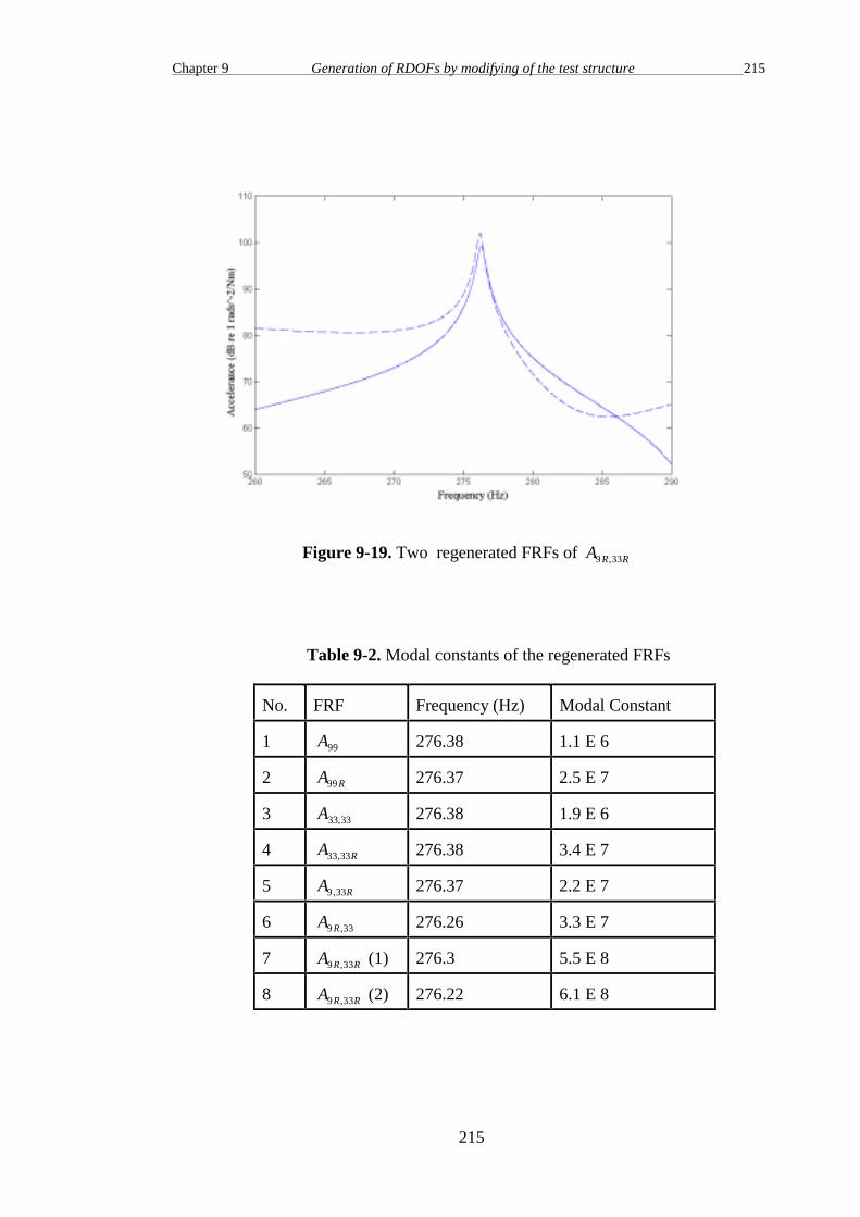
Chapter 9 Generation of RDOFs by modifying of the test structure 215
215
Figure 9-19. Two regenerated FRFs of A R R9 33,
Table 9-2. Modal constants of the regenerated FRFs
No. FRF Frequency (Hz) Modal Constant
1 A99 276.38 1.1 E 6
2 A R99 276.37 2.5 E 7
3 A33 33, 276.38 1.9 E 6
4 A R33 33, 276.38 3.4 E 7
5 A R9 33, 276.37 2.2 E 7
6 A R9 33, 276.26 3.3 E 7
7 A R R9 33, (1) 276.3 5.5 E 8
8 A R R9 33, (2) 276.22 6.1 E 8

Chapter 9 Generation of RDOFs by modifying of the test structure 216
216
9.4 Test strategy
In order to apply the method presented in this chapter for generating the rotational
FRFs the following procedure is suggested for the structure shown in Figure 9-20:
1. Obtain the mode shapes of the structure by conducting a conventional modal test
on the structure or by using the FE model of the structure.
2. Obtain the nodal points (translational and rotational) of the structure for a
particular mode from the corresponding mode shape. It should be noted that
rotational nodal points are obtainable using the finite difference technique.
3. Choose two points on the structure which are not close to the nodal points
(translational and rotational).
4. Select two additive elements with the same mass but different moments of inertia
so that by adding of them to the test structure considerable changes happen around
the resonance of the test structure. These additive elements should be chosen by
trial and error.
5. Check the behaviour of the modified structure for signs of nonlinearity.
6. Test the structure following the measurement technique stated in section 9.2.2.
7. Regenerate the measured FRFs using curve-fitting techniques to avoid the effects
of noise on the computations.
8. Generate the rotational FRFs following the procedure stated in section 9.2.3.
9. Check the results by conducting an internal check of generated FRFs using their
modal constants.

Chapter 9 Generation of RDOFs by modifying of the test structure 217
217
Figure 9-20. Generation of rotational FRFs of a structure
9.5 Conclusions
• In this chapter a method was presented for the generation of the transfer rotational
FRFs by modifying the test structure.
• It was shown the problem of the rotational excitation of the structure can be
eliminated by adding objects to the structure and using correction methods
presented in the previous chapters.
• The results of the theoretical simulation showed that the generated FRFs are
acceptable around the resonance area of the structure although some part of the
generated FRFs show considerable difference from the exact FRF due to the
approximate nature of the finite difference technique.
• The method was successfully applied to experimental data for a free-free beam
and the internal check of the generated FRFs demonstrated the validity of the
method.

Chapter 10 Conclusions 218
218
Conclusions and suggestions for future work
10.1 Conclusions
This section presents a summary of the conclusions of the work presented in this thesis.
10.1.1 Introduction
The sources of a lack of precision in modal testing have been categorised in three
groups: (i) experimental data acquisition errors (ii) signal processing errors and (iii)
modal analysis errors. This research was mostly dedicated to the first category of these
sources of errors and particularly on the sources of errors caused by mechanical devices
such as: accelerometers, suspension springs and stingers. A detailed literature survey
indicated that the current approach used to resolve the problems which these mechanical
errors cause is basically “avoidance” by choosing suitable test equipment so that the
probable errors become minimal.
A new trend to deal with the problem of the mechanical errors is calculating the exact
values of the FRFs by repeating the measurement in a number of different configuration;
each configuration consisting of the structure with one or more of its boundary
conditions changed . The main emphasis in this thesis was to use this trend in order to
develop new methods which permit the acquisition of data of high quality and to devise
methods to specify the accuracy of the measured data. However, further investigation
showed that this new trend is applicable in other fields such as generation of rotational
FRFs.
Chapter 10 Conclusions 219
219
10.1.2 The effects of mechanical devices on the measured FRFs
i) Correction of the mass-loading effects of transducers
A new method was developed for the correction of the mass-loading effects of the
transducers. It was shown that if an FRF measurement is repeated using another
accelerometer with a different mass, the exact value of the FRF can be obtained using a
series of straightforward calculations. Moreover, the driving point FRF at the point of
the attachment of the accelerometer is obtainable through this process. The method was
successfully applied to analytically-generated test cases and it was shown that, in the
presence of noise, this calculation becomes more sensitive to noise when the masses of
two accelerometers become closer together. Moreover, the method was successfully
applied to experimental data from test on a free-free beam. Based on this approach, a
new method was developed for estimating the exact natural frequencies of the structure.
A comparison between the exact natural frequencies of the structure and those of the
modified structure can show us the quality of the measurement. Moreover, it was shown
that the calibration of the measurement set-up can be checked using the method
presented for the correction of the mass-loading effects of transducers.
ii) Correction of the suspension effects in modal testing
A method similar to that developed for the correction of the mass-loading effects of the
transducers was developed for the correction of the effects of the suspension springs on
the measured FRFs. It was shown that for the simplest case where the test structure is
suspended from one spring, the FRFs can be corrected if the structure is tested three
times using different suspension springs with different stiffness in each test. Moreover,
the driving point FRF of the point of the attachment of the spring can be obtained
through the correction process. A numerical case study demonstrated the validity of the
method. However, in the presence of noise, as the suspension springs become stiffer, the
results of the presented correction method become more contaminated. The method was
successfully applied to the experimental data from tests on a cantilever beam. Further, an
approximate method was introduced to assess the quality of the measurement relating to

Chapter 10 Conclusions 220
220
the effects of the suspension spring based on the changes in the natural frequencies of
the structure.
iii) The effects of stingers on measured FRFs
It was proven that in a shaker test, the maximum error on the measured FRFs are
associated with the antiresonances of the rotational driving point receptance of the tip of
the stinger on the structure side. A new model was presented for the shaker-stinger-
structure system in which the test structure was considered as a rigid body that moves in
the transverse direction. This new model allowed us to assess the effect of misalignment
of the stinger on its performance. It was shown that when there is a misalignment
between two ends of the stinger, the antiresonances of the stinger shift to other
frequencies and the measured FRFs are biased. As a result, a maximum allowable
misalignment of the stinger was introduced based on the changes in the first elastic
antiresonance of the stinger. The presented model was used for the calculations of the
antiresonances of the shaker-stinger-structure system which was successfully validated
by the experimental measurements made on a free-free beam. Based on this study a
design procedure was introduced which followed by an example.
Moreover, it was shown that the effects of the stinger on the measured FRF can be
checked by repeating the test with another stinger with the same diameter but slightly
different length. A comparison between the measured FRFs using these two stingers
shows the possible errors due to the antiresonances of the stinger.
10.1.3 Correction in more than one DOF
When a test structure is modified in more than one DOF, the measured FRFs can be
corrected if the measurement is repeated in a number of different configurations; each
configuration consisting of the system with one or more of its boundary conditions
changed. Basically, two different approaches can be used for the correction of the effects
of the mechanical devices on the test structure in more than one DOF, namely the step
by step approach and the direct approach. In these approaches the driving point FRFs
related to the degrees of freedom of the attachment of mechanical devices can be

Chapter 10 Conclusions 221
221
computed without actually having to measure them. However, it was shown that the
direct approach produces meaningless results if the matrix which is built based on the
receptances of the attached objects is rank deficient.
This study provided a mathematical basis for the correction of the effects of the
mechanical elements on the test structure in more than one DOF. However, in practice,
applications of these methods are limited. The application of the methods presented in
this part of the research was in chapter 9 where the test structure was modified by the
mass and rotational inertia of an attached object in two DOFs in order to generate the
rotational FRFs.
10.1.4 The effect of nonlinearity on the correction methods of the
mechanical devices
The main assumption in the correction methods presented in this work is that the test
structure and the attached elements exhibit linear behaviour. In practice, real structures
are seldom linear. If the structure or the attached elements exhibits nonlinear behaviour,
correction methods show different results using different sets of data corresponding to
different configurations of the test structure. When a mechanical element is attached to a
structure, the additional mass and/or stiffness of the attached element acts as a passive
force. As a result, different mechanical elements produce different passive forces on the
nonlinear structures and the results of the correction are different for these mechanical
elements.
In practice, there are other sources of systematic errors, such as leakage and phase shift
between the force or acceleration signal which may produce the same effects on the
correction methods.
10.1.5 Generation of the whole translational FRFs from measurements
of one column
When the number of DOFs is large, measuring the whole FRF matrix is difficult. As a
result, the elements of one row or one column of the FRF matrix are measured and the

Chapter 10 Conclusions 222
222
rest of the FRFs are synthesised from the measured ones using the identified modal
properties. However, because of the limitation of the frequency range of the
measurement, estimation of the unmeasured FRFs is not accurate. Evaluating the whole
FRF matrix from measurement of some elements of the FRF matrix by modifying the
structure at its boundaries can eliminate the problem of out of range modes. A method
was developed to generate the all the translational FRFs using one accelerometer and
one dummy mass.
The equations which include the effects of noise on the computed FRFs show that by
increasing the mass of the accelerometer and that of the dummy mass, the effects of the
noise on the computation of the FRFs decreases. A numerical case study proved the
validity of the method. The method was successfully applied to the experimental data of
a free-free beam. However, the level of noise was considerable at the frequency points
out side the resonance regions.
10.1.6 Generation of the rotational FRFs by modifying the test
structure
The aim of this part of the research was to eliminate the need of applying the moment
excitation in order to generate rotational FRFs of the type displacement/moment and
rotation/moment using the correction methods presented in this work. It was proven that
in this procedure we still need to measure rotational responses. Therefore, Finite
difference technique and correction methods were used to develop a method in order to
generate the rotational FRFs related to two separate points on the structure.
The method was applied to an analytically-generated test case. The results were accurate
around the resonances of the analytical model but there were some errors in parts of the
frequency range due to the inaccuracy of the finite difference technique. In an actual test,
there are some potential problems due to the limitations of the experiment and should be
considered cautiously in the test. These problems are: selection of a suitable additive
object, nodal points, nonlinearity and noise. Nevertheless, the method was successfully
applied to experimental data for a free-free beam. The internal check of the generated
FRFs demonstrated that the method is valid and applicable.

Chapter 10 Conclusions 223
223
10.2 Recommended test strategy
It is usually prudent to carry out a preliminary limited modal test to help judge the
quality of the modal test and assess the nature of the structure being tested. Based on the
results of this preliminary test the measurement procedure can be planned. In the view of
the experience gained during this course of this research, and of the case studies
presented in this thesis, the following test strategy for the measurement with respect to
the mechanical devices errors is recommended.
i) Mass-loading effects of transducers on the measured FRFs
Add an extra mass to the accelerometer and assess the quality of the measurement by
estimating the exact natural frequencies of the modified structure as explained in chapter
3. For a mode of the structure, if there is an unacceptable difference between the
measured natural frequency and the exact natural frequency of the structure, use the
correction method presented in chapter 3 to cancel the effect of the accelerometer on the
measured FRFs.
ii) The effect of the suspension spring on the measured FRFs
Double the stiffness of the suspension spring and assess the quality of the measurement
by estimating the natural frequencies of the structure as explained in chapter 4. If the
quality of the measurement is not acceptable, reduce the stiffness of the suspension
spring or change the suspension point of the structure to another point or use the
correction method presented in chapter 4.
iii) The effect of the stingers on the measured FRFs
Design the stinger based on the maximum input force and the minimum and maximum
required measurement frequencies as was explained in chapter 5. Determine the
maximum allowable deformation of the stinger Test the structure using the designed
stinger considering the maximum allowable misalignment of the stinger. Check The
quality of the measurement by repeating the measurement using a stinger with the same
diameter but slightly different length.

Chapter 10 Conclusions 224
224
iv) The effects of the mechanical devices in more than one DOF
When the test structure is modified in more than one DOF (which is usually the case in
modal testing) the abovementioned test strategy for an individual mechanical device
should be accomplished for all of the modified DOFs one by one. Clearly when the
effect of a mechanical device on the measured FRFs at one DOF is reduced, the total
quality of the measurement improves. It is not recommended to use correction methods
for more than one DOF because as was shown in chapter 6 when the test structure is
modified in two DOFs at least 7 different measurements with different configurations
are needed to obtain the exact FRF. In practice, conducting this number of tests with
different configurations is not efficient. Moreover, the effects of noise and other errors
pollute the results of the correction due to the large number of the computation levels.
Instead, when the structure is affected unacceptably by suspension springs and an
accelerometer in more than one DOF, we can reduce the effect of the suspension springs
by using softer springs or changing the suspension points to the nodal points of the
modes of interest and use the correction method to cancel the mass-loading effect of the
accelerometer.
10.3 Summary of contributions of present work
A brief overview of contributions made in this thesis to the subject of ‘ High quality
modal testing methods’ is given here.
• A new idea to deal with mechanical errors was introduced and demonstrated using a
simple example (section 1.9).
• A detailed literature survey was carried out and all the major sources of a lack of
precision in the measurement process related to applied mechanical devices were
presented in a consistent notation (chapter 2).
• The problem of the mass-loading effect of transducers was revisited using the
SMURF method and a general solution for the correction of these mass-loading
effects of the transducers was presented. Based on this method, a new approach for

Chapter 10 Conclusions 225
225
assessing the quality of the measurement due to the mass-loading effect of the
transducers was suggested (chapter 3).
• The method for the correction of the mass-loading effect of transducers was used to
develop a new method to check the calibration of the measurement set-up (section
3-4).
• The problem of the suspension effects in modal testing was redefined using the
SMURF method and a correction method was developed for this case. Moreover, the
effect of noise on the computations was investigated (chapter 4).
• An approximate method was suggested to assess the quality of the measurement for
the case that the test structure is affected by one suspension spring (section 4.4).
• A new model was introduced for the shaker-stinger-structure system. This model
allowed us to assess the effect of the misalignment of the stinger on its performance
(section 5.3).
• A maximum allowable deformation for the stingers was introduced to avoid of
biasing the measured FRFs due to the deformation of the stinger (section 5.5).
• A new approach was introduced to assess the quality of the measurement due to the
effects of a stinger on the measured FRFs (section 5.6).
• For the case that the test structure is modified in more than one DOF, two different
approaches were suggested namely: step by step approach and direct approach.
Moreover, it was shown that in direct approach the results can be meaningless due to
the rank-deficiency problem (chapter 6).
• The effect of the nonlinearity on the correction methods of the mechanical devices
was investigated and it was shown that the results of the correction changes by using
different set of data corresponding to different configurations (chapter 7).
• Finite difference technique and the correction methods were applied for the
generation of the rotational FRFs and elimination of the need to apply moment
excitations (chapter 9).

Chapter 10 Conclusions 226
226
10.4 Suggestions for future studies
Whereas extensive research work on improving the acquisition of data in high quality of
modal testing has been carried out in this thesis, the study undertaken has revealed that
some further development may still be necessary and of interest. Areas for possible
further studies are summarised below:
• The correction methods can be investigated further to extend their applicability in
conventional modal testing.
• The success of the correction methods depends on the level of experimental noise,
and hence further developments of experimental equipment to reduce the level of
noise are of considerable importance. Development of a smoothing technique to
reduce the effect of experimental noise on the FRFs is required.
• Further investigation is necessary on the experimental determination of the
displacements (rotational and translational) in other DOFs following the techniques
suggested in present work on the experimental determination of rotational properties.
• The suggested correction methods allows us for the measurement of the modes
which are normally outside the measurement range. Investigation is necessary on this
topic to verify of potentially important out of range modes of the test structure.
• Another interesting topic to be investigated further relates to the determination of the
modal properties of the structures possessing close modes. In this case, the close
modes can be separated by modifying the test structure and then the measured FRFs
can be corrected using correction methods suggested in the present work.
• The correction methods presented in this work can be investigated further to extend
its applicability to the Multi-Input-Multi-output (MIMO) techniques.

Chapter 10 Conclusions 227
227
10.5 Closure
The primary aim of this work was to improve the current measurement techniques and to
develop new ones which permit the acquisition of data in high quality and to devise
methods to specify the accuracy of the measured data in a conventional modal test. This
was achieved by critical investigation of existing methods and by exploring new
techniques and a recommended test strategy has been presented in this thesis.
A summary of conclusions and contributions showed the advances made in the
measurement techniques. Not surprisingly, however, there is still scope for further study
to improve the accuracy of the measured data.

Appendix A
228
228
Appendix A
The effects of mechanical devices on the test structure
Reminder of Nomenclature
αij* measured receptance of a modified structure
′α ii receptance of the attached mechanical element at DOF i
1. Introduction
In this appendix the SMURF method is used to analyse the general case of the
modification of a test structure by mechanical devices. By mechanical devices we
mean the extraneous objects which are attached to the test structure to conduct the
modal test including suspension springs, transducers and stingers.
2. Modification of the test structure by mechanical devices
For the general case, a structure may be modified by addition of the mass and
rotational inertia of an attached object, a linear spring or a rotational spring. The
connection of these mechanical elements can be at any point on the structure and at
any DOF (Three translational DOFs and three rotational DOFs). Figure 1 indicates a
typical example of a structure which has been modified by mechanical elements. The
boxes are the indications of the extraneous systems which can be an axial spring, a
rotational spring, the mass property of an extraneous object , the rotational inertia
property of an extraneous object or a combination of them. Only the receptances of
the extraneous systems has been shown in the boxes. In Figure 1 numbers 1,2,3,4,5,6
and 7 refer to the number of modification DOFs.
In the system shown in Figure 1 structure C has been modified in the x direction at
DOFs 1, 3, 4 and 6. The structure has been modified in the y direction at DOF 5 and
in the z direction at DOF 2. At DOF 7, the structure has been modified rotationally in

Appendix A
229
229
the θ y direction. It is important to note that although for example DOFs 5 and 6 are at
the same point but they are different in direction. The structure is excited at DOF l in
the y direction and the response is measured at DOF k in the y direction. We show
displacements and rotations in all directions by X to derive the general form of the
equation of a modified structure.
Figure 1. A typical example of a modified structure
As is usually the case in modal testing, the structure and the additional systems are
presumed to be linear. For the general case, changes in a Frequency Response
Function (FRF) of a structure due to addition of extraneous objects can be computed
as follows :
The equations governing the modified system are :
X F R R R
X F R R R
X F R R R
X F R R R
l lk k l l n
k k n n
k k n n
n nk k n n nn n
= + + + ⋅ ⋅ ⋅ += + + + ⋅⋅ ⋅ += + + + ⋅ ⋅ ⋅ +
⋅ ⋅⋅ ⋅⋅ ⋅
= + + + ⋅ ⋅ ⋅ +
α α α αα α α αα α α α
α α α α
1 1 2 2
1 1 11 1 12 2 1
2 2 21 1 22 2 2
1 1 2 2
ln
(1)
The equations governing the additional systems are :

Appendix A
230
230
′ = ′ ′′ = ′ ′
⋅⋅⋅
′ = ′ ′
X R
X R
X Rn nn n
1 11 1
2 22 2
αα
α
(2)
The constraining equations are :
′ =′ =
⋅⋅⋅
′ =
X x
X x
X xn n
1 1
2 2
,
′ + =′ + =
⋅⋅⋅
′ + =
R R
R R
R Rn n
1 1
2 2
0
0
0
(3)
where X1 , X 2 , …, X n and X1’, X 2
’ , …, X n’ are unknown displacements or
rotations and R1 , R2 , …, Rn and R1’ , R2
’ , …, Rn’are unknown reaction forces. From
equations (2), (3) we have :
X R
X R
X Rn nn n
1 11 1
2 22 2
= − ′= − ′
= − ′
αα
α
.
.
.
(4)
Inserting equations (4) into equation (1) results in :

Appendix A
231
231
X F R R R
R F R R R
R F R R R
R F R R R
l lk k l l n
k k n n
k k n n
nn n nk k n n nn n
= + + + ⋅ ⋅ ⋅ +− ′ = + + + ⋅ ⋅ ⋅ +− ′ = + + + ⋅ ⋅ ⋅ +
⋅ ⋅⋅ ⋅⋅ ⋅
− ′ = + + + ⋅⋅ ⋅ +
α α α αα α α α αα α α α α
α α α α α
1 1 2 2
11 1 1 11 1 12 2 1
22 2 2 21 1 22 2 2
1 1 2 2
ln
(5)
or :
X F R R R
F R R R
F R R R
F R R R
l lk k l l n
k k n n
k k n n
nk k n n nn nn n
= + + + ⋅ ⋅ ⋅ += + + ′ + + ⋅⋅ ⋅ += + + + ′ + ⋅ ⋅ ⋅ +
⋅ ⋅⋅ ⋅⋅ ⋅
= + + + ⋅ ⋅ ⋅ + + ′
α α α αα α α α αα α α α α
α α α α α
1 1 2 2
1 11 11 1 12 2 1
2 21 1 22 22 2 2
1 1 2 2
0
0
0
ln
( )
( )
( )
(6)
Equation (6) can be written in matrix form as :
X F
R
R
R
l lk l l
k n
k n
nk n n nn nn
k
n
0
0
0
1 2
1 11 11 12 1
2 21 22 22 2
1 2
1
2
⋅⋅⋅
=
+ ′+ ′ ⋅ ⋅ ⋅
⋅ ⋅ ⋅ ⋅ ⋅⋅ ⋅ ⋅ ⋅ ⋅⋅ ⋅ ⋅ ⋅ ⋅
⋅ ⋅ ⋅ + ′
⋅⋅⋅
α α α αα α α α αα α α α α
α α α α α
. . .
. . .ln
(7)
If matrix [ ]α is defined as :
[ ]
. . .
. . .ln
α
α α α αα α α α αα α α α α
α α α α α
=
+ ′+ ′ ⋅ ⋅ ⋅
⋅ ⋅ ⋅ ⋅ ⋅⋅ ⋅ ⋅ ⋅ ⋅⋅ ⋅ ⋅ ⋅ ⋅
⋅ ⋅ ⋅ + ′
lk l l
k n
k n
nk n n nn nn
1 2
1 11 11 12 1
2 21 22 22 2
1 2
(8)
then:

Appendix A
232
232
[ ]
X F
R
R
R
l k
n
0
0
0
1
2
⋅⋅⋅
= ⋅⋅⋅
α (9)
To find a relation between X l and Fk , we have:
F
R
R
R
Xk
n
l
1
2
1
0
0
0
⋅⋅⋅
= ⋅⋅⋅
−[ ]α (10)
The inverse of [ ]α is :
[ ]α α− =
⋅ ⋅⋅ ⋅
⋅ ⋅ ⋅ ⋅ ⋅⋅ ⋅ ⋅ ⋅ ⋅
⋅ ⋅
1
11 12 1
21 22 2
1 2
1
c c c
c c c
c c c
n
n
n n nn
(11)
Inserting equation (11) in to (10) for the first row of the resulted equation we have:
cX Fl k
11
α=
(12)
or :
X
F cl
k
=α11
(13)
X
Fl
k
is simply α lk* , which is the measured receptance when the structure is modified
by extraneous mechanical devices.

Appendix A
233
233
αα
lk c* =
11
(14)
or :
α
α α α αα α α α αα α α α α
α α α α αα α α α
α α α α
α α α α
lk
lk l l
k n
k n
nk n n nn nn
n
n
n n nn nn
*
ln
=
⋅ ⋅+ ′ ⋅ ⋅
+ ′ ⋅ ⋅⋅ ⋅ ⋅ ⋅ ⋅ ⋅⋅ ⋅ ⋅ ⋅ ⋅ ⋅
⋅ ⋅ + ′+ ′ ⋅ ⋅
+ ′ ⋅ ⋅⋅ ⋅ ⋅ ⋅ ⋅⋅ ⋅ ⋅ ⋅ ⋅
⋅ ⋅ + ′
1 2
1 11 11 12 1
2 21 22 22 2
1 2
11 11 12 1
21 22 22 2
1 2
(15)
Equation (15) is the general equation for changes in the FRFs of a structure when it is
modified with different mechanical elements connected at different DOFs to the
structure.
As an example, when the structure is modified by two mechanical elements, Equation
(15) is simplified as [Chapter 4]:
α αα α α α α α
α α α α α αlk lkk k l* [ ( ) ]
( )( )= −
+ ′ −+ ′ + ′ −
2 11 11 21 1 2
22 22 11 11 12 21
+− + ′
+ ′ + ′ −[ ( )]
( )( )
α α α α α αα α α α α α
2 12 1 22 22 1
22 22 11 11 12 21
k k l
(16)
If these two extraneous elements are two masses the resulting equation is what was
driven in chapter 8, and if these elements are the mass and inertia of a T block, the
resulting equation is what was driven by Maia, Silva and Ribeiro in [37] using
coupling/uncoupling techniques. In both cases the form of the equation is the same as
equation (16). Therefore, what is important in this study is the form of the equation
and not the type of the extraneous elements.

Appendix B
234
234
Appendix B
Estimation of the FRFs of a grounded structure
In chapter 6 it was shown that how the measured FRFs of a structure which is affected
by mechanical devices can be corrected by modifying the structure at its boundaries.
The solution to this correction method produce FRFs of the structure with free-free
boundary condition. However, this solution can be applied for the estimation of other
boundary conditions. In this appendix the method suggested in chapter 6 is developed
to obtain the FRFs of the structure which is grounded at some of its degrees of
freedom.
The example of section 6.3.2 of is considered here again. From equation (6-27) for a
structure which is modified in two DOFs we have:
α79 71 1 2 2 3 3
4 1 5 2 6 3 4
= −+ +
+ + +x
x a x a x a
x a x a x a a( 1)
In which x’s are unknowns and a’s are known parameters.
Figure 1 shows a beam which has been grounded at DOF 3 (transverse direction) or in
other words has been pinned at point A.
Figure 1. Computation of the FRFs of a pinned beam using correction method
( TDOFs = Translational Degrees of Freedom , RDOFs = Rotational Degrees of Freedom )

Appendix B
235
235
When the receptance of the one of the extraneous elements in a DOF is zero it means
that the structure does not have any motion in that DOF or it is grounded on that
DOF. Conversely, when the receptance of one of the extraneous elements is ∞
(infinity) it means that the structure is free in that DOF. To ground DOF 3, while
DOF 4 is free, the conditions are:
′ =′ = ∞
αα
33
44
0(2)
from equation (6-27) we had:
a
a
a
a
1
2 33
3 44
4 33 44
1== ′= ′
= ′ ′
αα
α α
(3)
Inserting (3) in ( 1), the result is :
αα α
α α α α79 71 2 33 3 44
4 5 33 6 44 33 44
= −+ ′ + ′
+ ′ + ′ + ′ ′x
x x x
x x x
( ) ( )
( ) ( ) ( )
(4)
Now if conditions (2) is applied in equation (4), we have:
α97 73
6
g xx
x= −
(5)
in which α97g refers to the FRF of grounded structure. Figure 2 shows the comparison
of the exact FRF of the pinned beam which is computed by the elimination of the
DOF 3 in the impedance matrix of the beam and the computed FRF using equation
(5) and the answers to the equation ( 1) in chapter 6.

Appendix B
236
236
Figure 2. Comparison of the Computed FRF of the grounded
structure and the exact FRF
In this appendix, the correction method suggested in chapter 6 has been developed to
produce grounded condition of a test structure by a series of different configurations
of the test structure. The method is more reliable than conventional test of a grounded
structure because the test structure with the unknown boundary conditions is replaced
by a known boundary condition which does not contaminate the modal test results
with fixture coupled modes or boundary condition uncertainties.

Appendix C
237
237
Matrix Properties
1. Matrix norms
The norm of a matrix is a function of the elements of that matrix which reflects the
“size” of the matrix. The most common matrix norms are the Frobenious norms,
A aF ijj
N
i
M
=
==∑∑
2
11
12 (1)
and
A F n2
12
22 2= + + ⋅ ⋅ ⋅ +σ σ σ
(2)
where σ i are the singular values of [A].
and the p-norms,
AAx
xpx
p
p
=≠
sup0
(3)
from where,
A aj
iji
M
11
==∑max
(4)
A ai
ijj
N
∞=
= ∑max1
(5)
and

Appendix C
238
238
A 2 = [max. eigenvalue ][ ] [ ]A AT1
2 =σ 1(6)
An important property of the Frobenious norms is that they are invariant with respect
to orthogonal transformations. Thus orthogonal transformations just rotate the original
matrix without changing its norm.
2. The rank of a matrix
The rank of a matrix ( r ) is the number of linearly independent rows (and columns) in
a given matrix. Some of the rank properties of a matrix are:
1. r is a positive integer;
2. when the rank of a square matrix is equal to its number of rows (or columns), then
the matrix is non-singular i.e., its inverse exists and is said to have full rank
3. when a matrix is not square, the rank of that matrix equals or is less than the
smaller of its number of rows or columns.
4. when the rank of a matrix is not zero, there is at least one square submatrix of
that matrix having order of r ( rank of the matrix ) and is not singular.
2. The Singular Value Decomposition (SVD)
The SVD of an m n× real matrix [A] is expressed by:
[ ] [ ] [ ] [ ]A U Vm n m m m n n nT
× × × ×= Σ (7)
where [U] and [V] are orthogonal matrices , i.e :
[ ] [ ] [ ][ ] [ ] [ ] [ ][ ] [ ]U U U U V V V V IT T T T= = = = (8)
and
[ ] [ ]U UT = −1 and [ ] [ ]V VT = −1 (9)

Appendix C
239
239
[ ]Σ is a real matrix with elements σ σij i= for i=j and σ ij = 0 for i j≠ . The values
σ i are called singular values of matrix [A]. Singular values can be arrenged in
decreasing order (σ σ σ1 2> > ⋅⋅ ⋅ > N ). Thus:
[ ]Σ =
⋅⋅
⋅ ⋅ ⋅ ⋅⋅
− − − −⋅
×
σσ
σ
1
2
0 0
0 0
0 0
0 0 0
n
m n
(10)
The value of the rank is equal to the number of nonzero singular values. The
advantage of using the SVD to calculate the rank is that if a row is not totally linearly
dependent instead of zero a small value for the smallest singular value will be
obtained and we have to compare this small value with the other singular values. A
reasonable criterion for the acceptance or rejection of small singular values is to
calculate the consecutive ratios of the singular values, σ σ1 2/ , σ σ2 3/ , … , σ σn n−1 /
If some of these ratios are very small compared with the others, they are not
acceptable.
If [A] is a complex matrix, then equation (7) becomes:
[ ] [ ] [ ] [ ]A U Vm n m m m n n nH
× × × ×= Σ (11)
where the superscript H denotes complex conjugate (hermitian) transpose. Now [U]
and [V] are unitary instead of orthogonal, i.e:
[ ] [ ] [ ][ ] [ ] [ ] [ ][ ] [ ]U U U U V V V V IH H H H= = = = (12)
[ ] [ ]U UH = −1 and [ ] [ ]V VH = −1 (13)
The singular values of a complex matrix, [ ]A , are the non-negative square-roots of
the eigenvalues of the matrix [ ] [ ]A AH and are always real.

Appendix C
240
240
3. Condition Number
In general, matrices are not diagonal but using SVD, we have the product of two
orthogonal matrices and a diagonal one. As orthogonal matrices preserve norm , the
norm of a matrix will be the norm of matrix [ ]Σ in the SVD. So, the matrix of the
singular values can give us an indication about ill-conditioning. The ratio of
σ σmin max/ is an indicator of potential computational problems. The condition number
of a matrix is the ratio σ σmin max/ . whereσ max is the largest singular value and σ min is
the smallest non-zero singular value of the matrix. A high condition number reflects
an ill-conditioned matrix.
4. The Pseudo-inverse of a matrix
The matrix [ ]A n m+
× is called pseudo-inverse of the matrix [ ]A m n× if the following
conditions are satisfied:
1. [ ][ ] [ ] [ ]A A A A+ =
2. [ ] [ ][ ] [ ]A A A A+ + +=
3. [ ][ ]A A + is symmetric
4. [ ] [ ]A A+ is symmetric
If [A] is square and non-singular, then [ ] [ ]A A+ −= 1 . The pseudo-inverse is related to
the least-square problem , as the value of { }x that minimizes [ ]{ } { }A x b−2 in
equation [ ] { } { }A x bm n n m× × ×=1 1 . This can be given by { } [ ] { }x A b= + .

Appendix D
241
241
The ANSYS model of the stinger
/ The model of the stinger
/FILNAM,beam-b
/TITLE,Stinger
/prep7
/com M1 = mass of the structure
/com J1 = second moment of inertia of the structure
M1=10.5
J1=0
/com M2 = total mass of the shaker for non-axial vibrations
/com of the stinger and the mass of the coil of the shaker
/com for the axial vibration
/com J2 = second moment of inertia of the total mass of the shaker for
/com non-axial vibrations of the stinger and second moment of inertia
/com of the mass of the coil of the shaker for the axial vibration
M2=0.02
J2=0.001
/com K1 = Suspension stiffness of the structure
/com K2 = Suspension stiffness of the shaker
/com KT2 = Rotational suspension stiffness of the shaker
K1=850
K2=1400

Appendix D
242
242
KT2=0.469
/com L = lenght of the stinger
/com A = Cross sectional area of the stinger
/com I = Second moment of inertia of the stinger
/com h = height of the beam
L=.1
A=3.1416E-6
I=7.854E-13
h=.002
KAN,2
KAY,2,50
KAY,3,0
/com EX = modolus of elasticity of the stinger
/com DENS = Mass density of the stinger
ET,1,3
R,1,A,I,h
EX,1,210E9
DENS,1,7800
N,1,0,0,0
N,101,L,0,0
FILL

Appendix D
243
243
N,102,L,0.3,0
N,103,0,0.3,0
N,104,0,0,0
REAL,1
E,1,2
EGEN,100,1,1
ET,5,21
KEYOPT,5,3,3
KEYOPT,5,2,0
R,8,M1,J1
TYPE,5
REAL,8
E,101
ET,6,21
KEYOPT,6,3,3
R,9,M2,J2
TYPE,6
REAL,9
E,1
ET,2,14
KEYOPT,2,3,2
R,2,K1

Appendix D
244
244
TYPE,2
REAL,2
E,101,102
R,3,K2
TYPE,2
REAL,3
E,1,103
ET,7,14
KEYOPT,7,2,6
R,4,KT1
TYPE,7
REAL,4
E,1,104
F,101,MZ,1.25
D,103,ALL,0
D,102,ALL,0
D,104,ALL,0
TOTAL,200
ITER,1,1,1
FINISH

References 245
245
References
[1] Blevins, R. D. : “Formulas for Natural Frequency and Mode Shape”. Van
Nostrand Reinfold Company, 1979.
[2] Cook, R. D. : “Concepts and Applications of Finite Element Analysis” John
Wiley and Sons, 2nd edition, 1981.
[3] Bathe, K-L : “Finite Element Procedures in Engineering Analysis” Prentice-
Hall, 1982.
[4] Zienkiewicz, O. C. and Taylor, R. L. : “The Finite Element Method” MacGraw-
Hill 4th edition, 1986.
[5] Ewins, D.J., : “Modal Testing : Theory and Practice”. John Willey & Sons,
London, 1984.
[6] Ewins, D.J. : “State-of-the-Art Assessment of mobility Measurement Techniques
(SAMM)”. Journal of Soc. Env. Engrs., pages 1-11, March 1981.
[7] Ewins, D.J. and Imergun, M. : “State-of-the-Art Assessment of Structural
Dynamic Response Analysis Methods (DYNAS)”, Shock and Vibration Bulletin,
56(1), August 1986.
[8] Harwood N. : “Quality Assurance In Dynamic Testing”. Proceeding of the !5th
Seminar on Modal analysis Leuven, Sep. 1990.
[9] Jung, H. and Ewins, D.J. : “On the Use of Simulated “Experimental” Data for
Evaluation of Modal Analysis Methods” . Proceeding of the 10th International Modal
Analysis Conference, pages 421-429,1992.
[10] Marudachalam, Kannan and Whicks, A.L. :“An Attempt to Quantify the
Errors in the Experimental Modal Analysis Process”. Proceeding of the 9th
International Modal Analysis Conference, pages 1522-1527,1991.

References 246
246
[11] Mitchell, L. D and Randolph, L. S. : “Modal Tests Methods : Quality,
Quantity, and Unobtainable” NAFEMS, International Conference Structural
Dynamics Modelling Test, Analysis and Correlation.
[12] Mitchell, L. D. and Elliot, K. B., : “Structural Modification Utilizing Beam
Elements”. Proceedings of the International Modal Analysis conference V, IMAC-V,
Volume II, Imperial College of Science and Technology, London, England, pp. 956-
959, April 6-9, 1987.
[13] Mitchell, L. D. and Elliot, K. B. : “The effect of Modal Truncation on Modal
Modification”. Proceeding of the International Modal Analysis Conference V, IMAC-
V, Volume I, Imperial College of Science and Technology, London, England, pp. 72-
78, April 6-9, 1987.
[14] Mitchell, L. D. and LUK Y. W., : “ Implementation of the Dual Modal Space
Structural Modification Method”. Proceeding of the International Modal Analysis
Conference II, IMAC II, Orlando, Florida, Published by Union College, Schenectady,
NY, PP. 930-936, February 6-9,1984.
[15] DTA Handbook, “Attachment of Excitation Device : Drive rods”. ITEM 32.3
M, pp.1-6, 11 Oct, 1994.
[16] Mitchell, L. D.,and Elliott, K. B., : “How to Design Stingers for Vibration
Testing of Structures”. Sounds and Vibration, pp.14-18, April 1984.
[17] Mitchell, L. D.,and Elliott, K. B., : “A Method for Designing Stingers for Use
in Mobility Testing”. Proceedings of the 2nd International Modal Analysis
Conference, pp. 872-876, 1984.
[18] Hieber, G. M., : “Non-Toxic Stingers”. Proceedings of the 6th International
Modal Analysis Conference, pp. 1371-1379, 1984.
[19] Chiang Lee, J. and Fang Chou, Y., : “The Effects of Stingers on Modal
Testing”. Proceedings of the 11th International Modal Analysis Conference, pp. 293-
299, 1993.

References 247
247
[20] Chiang Lee, J. and Fang Chou, Y., : “The Effects of Stingers on Recptance
Function Measurement”. Transactions of the ASME, pp. 220-226.
[21] McConnell, K. G., Zander, E., Dong, J. and Thekentattil, S., : “Effect of
Stinger Stiffness on Measured Accelerance” . Proceedings of the 15th International
Modal Analysis Conference, pp. 672-678 , 1997.
[22] Anderson, I.A., : “Avoiding Stinger Rod Resonance Effects on Small
Structures”. Proceedings of the 8th International Modal Analysis Conference, pp. 673-
678, 1990.
[23] Billhart, R. D. & Hunt, D. L. & Pierre, M. S. : “Advantages of Excitation
Using Plastic Stinger Rods”. Proceedings of the 11th International Modal Analysis
Conference, pp. 1217-1220, 1993.
[24] Han, S., : “Analysis on Natural Frequency Distortion Due to the Attachment of
Shaker”. Proceedings of the 13th International Modal Analysis Conference, pp. 1715-
1721, 1995.
[25] Vandepitte, D. V. ,Olbrechts, T. and Sas, P. : “FRF Measurements Errors
Caused by The Use of Inertia Mass Shaker”. Proceedings of the 15th International
Modal Analysis Conference, pp. 188-194 , 1997.
[26] McConnell, K. G. and Hu, X. : “Stinger mass compensation Part One :
Theoretical study & Part Two : Experimental Investigation”. Modal Analysis: the
International Journal of Analytical and Experimental Modal Analysis, V8 & n1, p.
35-44, p. 45-54, Jan 1993.
[27] McConnell, K. G. and Hu, X. : “An Advanced Model for Stinger Force, Motion
and Energy Transmissibilities”. Modal Analysis: the International Journal of
Analytical and Experimental Modal Analysis, V7 & n4, p. 271-283, Oct 1992.
[28] Olsen, N. L., “Using and Understanding Electrodynamic Shakers in Modal
Application”. Proceedings of the 4th International Modal Analysis Conference, pp.
1160-1167 , 1986.

References 248
248
[29] Peterson, E. L., Mouch, T. A., and Rusen, W. M., : “Modal Excitation : Force
Drop-Off at Resonances”. Proceedings of the 8th International Modal Analysis
Conference, pp. 1226-1231 , 1990.
[30] Rao, D. K., “Electrodynamic Interaction Between a Resonating Structure and an
Exciter” . Proceedings of the 5th International Modal Analysis Conference, pp. 1142-
1150 , 1987.
[31] Tomlinson, G. R., “A Simple Theoretical and Experimental Study of the Force
Characteristics from Electrodynamic Exciters on Linear and Non-linear Systems”.
Proceedings of the 8th International Modal Analysis Conference, pp. 1479-1486 ,
1987.
[32] Synder, V. W., : “Structural Modifications and Modal Analysis”. Proceedings
for Experimental Stress Analysis, 1983.
[33] Avitabile, P. and O’Callahan, J., : “Understanding Truncation Effects in
Structural Dynamic Modification”. Sound and Vibration, June 1990.
[34] Ole Dossing, : “Prediction of Transducer Mass-Loading Effects and
Identification of Dynamic Mass”. Proceedings of the 9th International Modal Analysis
Conference, pp. 306-312 , 1991.
[35] Decker, J. and Witfeid, H : “Correction of Transducer-Loading Effects in
Experimental Modal Analysis” . Proceedings of the 13th International Modal Analysis
Conference, pp. 1604-1608 , 1995.
[36] Silva, J. M. M., Maia, N. M. M. and Ribeiro, A. M. R., : “Some Applications
of Coupling/Uncoupling Techniques in Structural Dynamics, Part 1 : Solving the
Mass Cancellation Problem” . Proceedings of the 15th International Modal Analysis
Conference, pp. 1431-1439 , 1997.
[37] Silva, J. M. M., Maia, N. M. M. and Ribeiro, A. M. R., : “Some Applications
of Coupling/Uncoupling Techniques in Structural Dynamics, Part 1 : Generation of
the Whole FRF Matrix from measurements on a Single Column-The Mass Uncoupling

References 249
249
Method (MUM)” . Proceedings of the 15th International Modal Analysis Conference,
pp. 1440-1452 , 1997.
[38] Bisplinghoff, R. L., Ashley, H., & Halfman, R.L., “Elasticity”, Addison-
Wsley Publishing Company, Inc., Cambridge, MA, pp. 771-779.
[39] Strutt, J. W. (Lord Ryleigh), “The Theory of Sound” Vol.1, 2nd ed., Dover
Publications, Inc., Newyork, 1945.
[40] Wolf Jr., J.A., “The Influence of Mounting Stiffness on Frequencies Measured
in a Vibration Test”, SAE Paper 840480, Society of Automotive Engineers, 1984.
[41] Carne, G.T., & Dohrmann, C. R., : “Support Conditions, Their Effect on
Measured Modal Parameters” Proceedings of the 16th International Modal Analysis
Conference, pp. 477-483 , 1998.
[42] Lindholm,B. E. and West, R. L. : “Determination of Suspension Effects by
Direct Experiments and Comparisons to an Analytical Model” . Proceedings of the
12th International Modal Analysis Conference, pp. 262-268 , 1994.
[43] Simley, R. G. and Brinkman, B. A. : “Rotational Degrees-of-Freedom in
Structural Modification”. Proceedings of the 2th International Modal Analysis
Conference, pp. 937-939 , 1984.
[44] Wade, B., Kuo, C., Glaser, R : “Extension of Ground-Based Testing for Large
Space Structures”, Journal of Spacecraft and Rockets, Vol. 23, No. 2, pp. 184-188,
1986.
[45] Wade, B.,Kuo, C., Glaser, R., : “Multiple Boundary Condition Test (PBC)
Approach to Update Mathematical Models of Large Flexible Structures”. SAE Paper
851933, Oct 14-17,1985.
[46] Kuo, C., Wade, B. : “More About Multiple-Boundary-Condition Testing”, Nasa
Tech Brief, Vol. 14, NO 1, Item 16,JPL Invention Report NPO-17574/7082, January,
1990.

References 250
250
[47] Glaser, R., Kuo, C., Wade, B., : “ Improvement of Structural Models Using
Covariance Analysis and Nonlinear Generalised Least Squares”, AIAA Journal, Vol.
30, No. 1, pp. 226-233, 1992.
[48] Anderson, J. B. & Coleman, A. D. & Driskill, T. C. & Brown, D. L., : “A
Mass Additive Technique for Modal Testing as Applied to the Space Shuttle Atro-1
Payload” . Proceedings of the 6th International Modal Analysis Conference, pp. 154-
159 , 1988.
[49] Gwinn, K., Lauffer, J.and Miller, A. : “Component Mode Synthesis Using
Experimental Modes Enhanced by Mass Loading” . Proceedings of the 6th
International Modal Analysis Conference, pp. 1088-1093 , 1988.
[50] Lammens, S., Sas, P., Brown, D. L. : “Model Updating and Perturbed
Boundary Condition Testing”, Proceedings of the 17th International Seminar on
Modal Analysis, 1992.
[51] Chen, K. N., Brown, D. L., Nicolas, V. T., : “Perturbed Boundary Condition
Model Updating” . Proceedings of the 11th International Modal Analysis Conference,
1993.
[52] Barney, P., Pierre, M. S., Brown, D. L., : “ Identification of a Modal Model
Utilizing a Perturbed Boundary Condition Test Method” . Proceedings of the 10th
International Modal Analysis Conference, pp. 1221-1231 , 1992.
[53] Li, S., Brown, D. and Vold, H., : “Using the Scaled Total Least Squares
Method and Unified Matrix Polynomial Approach for Condensing the Perturbed
Boundary Condition Test Data”. Proceedings of the 13th International Modal
Analysis Conference, 1995.
[54] Anonymous, Kistler Piezo-Instrumentation, Catalog K2.006, Kistler
Instrument Corp., Amherst, NY, p.46, September 1989.

References 251
251
[55] Sainsbury, M. G., : “Vibration Analysis of Damped Complex Structures”. PhD
Thesis, Imperial College, University of London, 1976.
[56] Silva, J. M. M. : “Measurement and Applications of Structural Mobility Data
for the Vibration Analysis of Complex Structures” . PhD Thesis, Imperial College,
University of London, 1987.
[57] Ewins, D.J. and Sainsbury, M.G. : “Mobility Measurements for the vibration
Analysis of Connected Structures” Shock and Vibration Bulletin, 42(1), pp.105-122,
1972.
[58] Gleeson, P.T. : “Identification of Spatial Models”. PhD Thesis, Imperial
College, University of London, 1979.
[59] Skingle, G. W., : “Structural Dynamic Modification Using Experimental Data”
PhD Thesis, Imperial College, University of London, 1989.
[60] Urgeria, A.P.V., : “Dynamic Analysis of Coupled Structures Using
Experimental Data”. PhD Thesis, Imperial College, University of London, 1989.
[61] Chen, W. H. ; Cherg, J. S. : “Modal Synthesis Via Combined Experimental and
Finite Element Techniques with Consideration of Rotational Effects”. Journal of
Sound and Vibration, vol 103 (1), 1985.
[62] Sattinger, S.S., : “A method for Experimentally Determining Rotational
Mobilities of Structures” . Shock and Vibration Bulletin, 50 (1), 1980.
[63] Smiley, R. G. and Brinkman, B. A., : “Rotational Degrees-of-Freedom in
Structural Modification”. Proceedings of the 2nd International Modal Analysis
Conference, pp. 937-939, 1984.
[64] Liorca, F; Gerard, A. and Brenot, D., : “Improving Interface Conditions in
Modal Synthesis Methods. Application to a Bolted Assembly of Rectangular Plates”.
Proceedings of the 12th International Modal Analysis Conference, pp. 411-417, 1994.

References 252
252
[65] O’Callahan, J. C. ; Lieu, I. W. and Chou, C. M. : “Determination of
Rotational Degrees-of-Freedom for Moment Transfers in Structural Modification”.
Proceedings of the 3rd International Modal Analysis Conference, pp. 465-470, 1985.
[66] Williams, E. J. and Green, J. S., : “A Spatial Curve Fitting Technique for
Estimation of Rotational Degrees of Freedom”. Proceedings of the 8th International
Modal Analysis Conference, pp. 376-381, 1990.
[67] Haisty, B. S., and Springer, W. T., : “A Simplified Method for Extracting
Rotational Degrees-of-Freedom Information from Modal Test Data” IJAEMA, 1(3),
pp. 35-39 (1986).
[68] Ng’ andu, A. N., FOX, C. H. J. and Williams, E. J., : “On the Estimation of
Rotational Degrees-of Freedom Using Spline Functions” . Proceedings of the 13th
International Modal Analysis Conference, pp. 791-797, 1995.
[69] Leschiutta, M., Eng, J. A. and Martin, J. K., : “Dynamic Piston Measurements
Using a Laser Range-Finding Technique”. SAE Technical Paper Series, No. 900482,
1990.
[70] wang, W. and Bush-Vishniac, I., “Four Dimensional Non-contacting Sensing
System for Micro-Automation Machines” . ASME Paper no.90-WA/DSC-23A.,
1990.
[71] Cafeo, J. A., Trethewey, M. W., Rieker, J. R. and Sommer, H. J., :
“Application of a Three Degree of Freedom Laser Vibrometer for Experimental
Modal Analysis” . Proceedings of the 9th International Modal Analysis Conference,
pp. 1161-1167, 1991.
[72] Bokelberg, E. H., Sommer, H. J., and Trethewey, M. W., : “A Six-Degree-of-
Freedom Laser Vibrometer. Part I : Theoretical Development & Part II :
Experimental Validation” . Journal of Sound and Vibration 178(5), pp. 643-654,
1994.

References 253
253
[73] Huffaker, R. M., “Laser Doppler Detection Systems for Gas Velocity
Measurement”, Applied Optics, Vol.9, No.5,May 1970.
[74] Donavan, J. B., “Three-Dimensional Vibrometry via Three Positions of a One-
Dimentional Laser Doppler Velocimeter”, Master Thesis, Virginia Polytechnic
Institute and State University, Blacksburg, VA, 1991.
[75] Mitchell, L. D. and Abel, J. J., : “Extraction of In-Plane Velocities Using
Laser Doppler Velocimetry” . Proceedings of the 11th International Modal Analysis
Conference, pp. 402-408, 1993.
[76] Mitchell, L. D., and Galaitsis, G. S., : “Extraction of Drilling-Angular
Velocities Using a Nodal-Spatial Array of In-Plane, Translational Laser-Derived
Velocities”. ……pp.735-741.
[77] Kochersberger, K., Mitchell, L. D., and Wicks, A. L., : “Structural Angular
Velocity Extraction Using DFT/IDFT Techniques” . Proceedings of the 9th
International Modal Analysis Conference, pp. 657-663, 1991.
[78] Sun, F. P., and Mitchell, L. D., “Two-Dimensional Velocity Data Smoothing
and Structural Angular Velocity Extraction Using a DFT-IDFT Technique” .
Proceedings of the 13th Biennial ASME Conference on Mechanical Vibration and
Noise, pp. 303-309, 1991.
[79] Lindoholm, B. E., : “Three-Dimensional Position Registration of a Scanning
Laser-Doppler Vibrometer” .
[80] Stanbridge, A. B., and Ewins, D. J., : “Using a Continuously-Scanning Laser
Doppler Vibrometer for Modal Testing” . Proceedings of the 14th International Modal
Analysis Conference, 1996.
[81] Stanbridge, A. B., and Ewins, D. J., : “Modal Testing of Rotating Discs Using
a Scanning LDV” . Proc. ASME Design Engineering Technical Conference, Boston,
DE- Vol. 84-2, Vol.3B.

References 254
254
[82] Stanbridge, A. B., and Ewins, D. J., : “Structural Modal Analysis Using a
Scanning Laser Doppler Vibrometer” . R. Ae. Soc. Forum on Aeroelasticity and
Structural Dynamics, Manchester, 1995.
[83] Stanbridge, A. B., and Ewins, D. J., : “Measurement of Total Vibration at a
Point Using a Conical-Scanning LDV” . Proc. of ANCONA, 1996.
[84] Bendat, J. S., and Piersol, A. G., : “Random Data : Analysis and Measurement
Procedures” . Jhon Wiley and Sons, Wiley-Interscience, NewYork, NY,pp. 408-409,
1986.
[85] Mitchell, L. D., “ Improved Methods for the Fast Fourier Transform (FFT)
Calculation of the Frequency Response Function” . Journal of Mechanical Design,
Transactions of the ASME, pp. 277-279, Vol. 104, April 1982.
[86] Wicks, A. L., and Vold, H., : “The Hs Frequency Response Function
Estimator” . Proceedings of the 4th International Modal Analysis Conference, 1986.
[87] Wicks, A. L., and Mitchell, L. D., : “Methods for Estimation of Frequency
Response Functions in the Presence of Uncorrelated Noise, A Review”. International
Journal of Analytical and Experimental Modal Analysis, Vol. 2, No.3, pp. 109-112,
July 1987.
[88] Wicks, A. L., and Shapton, W. S., “A Comparison of H1 and H2 Frequency
Response Functions” . Society of Experimental Mechanics, Fall Annual Meeting,
Milwaukee, WI, November 1984.
[89] Vold, H., Rocklin, G. T., and Crowly, J., “A comparison of H1 , H2 ,
Hv Frequency Response Functions” . International Modal Analysis Conference
Proceedings, Orlando,FL, pp. 272-278, November 1984.
[90] Goyder, H. G. D., “Foolproof Methods for Frequency Response Measurement”
. Proceedings of the Second International Conference on Recent Advances in
Structural Dynamics, Southampton, England, 1984.

References 255
255
[91] Cobb, R. E., and Mitchell, L. D., “Estimates of Variance and Confidence
Bands for the three-Channel Frequency Response Function Estimator” . international
Journal of Analytical and Experimental Modal Analysis, Vol. 5., No.3,pp. 185-194,
July 1990.
[92] Cobb, R. E., and Mitchell, L. D., “Estimation of Uncorrelated Content in
Experimentally Measured Frequency Response Functions Using Three Measurement
Channels” . Mechanical Systems and Signal Processing, Vol. 4, No.6, pp. 449-461,
Nov.-Dec., 1990.
[93] Ashory, M. R. : “ Correction of Mass Loading Effects of Transducers and
Suspension Effects in Modal Testing” Proceeding of the 16th International Modal
Analysis Conference, pp. 815-828, 1998.
[94] McConnell, G. M., : “Vibration Testing : Theory and Practice” JhonWiley &
Sons, Inc., 1995.
[95] Klosterman, A. : “On the Experimental Determination and Use of Modal
Representations of Dynamic Characteristics”. PhD Dissertation, University of
Cincinnati, 1971.
[96] Bishop, R. E. D. and Johnson, D. C. : “The Mechanics of Vibration”.
Cambridge at the University Press, 1960.
[97] Blevins, R. : “Formulas for natural frequency and mode shape” Krieger
Publishing Company, Malabar, Florida.
[98] Fraleigh, J. B. and Beauregard, R. A. : “Linear Algebra”. Addison-Wesely
Publishing Company, 1995.
[99] McConnell, K. G. and Hu, X. : “Why do Large FRF Errors Result from Small
Relative Phase Shifts When Using Force Transducer Mass Compensation Methods?”
Proceedings of the 11th International Modal Analysis Conference, pp. 845-849 , 1993.

References 256
256
[100] Ashory, M. R. and D. J. Ewins : “Generation of the Whole FRF Matrix from
Measurements on One Column ” Proceeding of the 16th International Modal Analysis
Conference, pp. 800-814, 1998.
[101] Silva, J. M. M., Maia, N. M. M. and Ribeiro, A. M. R., : “Some Applications
of Coupling/Uncoupling Techniques in Structural Dynamics, Part III : Estimation of
Rotational Frequency Response Functions Using MUM)” . Proceedings of the 15th
International Modal Analysis Conference, pp. 1453-1462 , 1997.
[102] Duarte, M. L. M., : “Experimentally-Derived Structural Models for Use in
Further Dynamic Analysis” PhD Thesis, Imperial College, University of London,
1996.