High Performance Python (fromTraining at EuroPython 2011)

Release 0.2

Ian Ozsvald (@ianozsvald)

July 24, 2011

CONTENTS

1 Testimonials from EuroPython 2011 2

2 Motivation 42.1 Changelog . . . . . . . . . . . . . . . . . . . . . . . . . . . . . . . . . . . . . . . . . . . . . . . . 42.2 Credits . . . . . . . . . . . . . . . . . . . . . . . . . . . . . . . . . . . . . . . . . . . . . . . . . . 42.3 Other talks . . . . . . . . . . . . . . . . . . . . . . . . . . . . . . . . . . . . . . . . . . . . . . . . 5

3 The Mandelbrot problem 6

4 Goal 84.1 MacBook Core2Duo 2.0GHz . . . . . . . . . . . . . . . . . . . . . . . . . . . . . . . . . . . . . . 84.2 2.9GHz i3 desktop with GTX 480 GPU . . . . . . . . . . . . . . . . . . . . . . . . . . . . . . . . . 11

5 Using this as a tutorial 13

6 Versions and dependencies 14

7 Pure Python (CPython) implementation 15

8 Profiling with cProfile and line_profiler 18

9 Bytecode analysis 21

10 A (slightly) faster CPython implementation 22

11 PyPy 2411.1 numpy . . . . . . . . . . . . . . . . . . . . . . . . . . . . . . . . . . . . . . . . . . . . . . . . . . 24

12 Psyco 26

13 Cython 2713.1 Compiler directives . . . . . . . . . . . . . . . . . . . . . . . . . . . . . . . . . . . . . . . . . . . . 3013.2 prange . . . . . . . . . . . . . . . . . . . . . . . . . . . . . . . . . . . . . . . . . . . . . . . . . . 31

14 Cython with numpy arrays 32

15 ShedSkin 3315.1 Profiling . . . . . . . . . . . . . . . . . . . . . . . . . . . . . . . . . . . . . . . . . . . . . . . . . 3415.2 Faster code . . . . . . . . . . . . . . . . . . . . . . . . . . . . . . . . . . . . . . . . . . . . . . . . 34

16 numpy vectors 35

i

17 numpy vectors and cache considerations 37

18 NumExpr on numpy vectors 39

19 pyCUDA 4119.1 numpy-like interface . . . . . . . . . . . . . . . . . . . . . . . . . . . . . . . . . . . . . . . . . . . 4219.2 ElementWise . . . . . . . . . . . . . . . . . . . . . . . . . . . . . . . . . . . . . . . . . . . . . . . 4319.3 SourceModule . . . . . . . . . . . . . . . . . . . . . . . . . . . . . . . . . . . . . . . . . . . . . . 44

20 multiprocessing 46

21 ParallelPython 48

22 Other ways to make things run faster 5022.1 Algorithmic choices . . . . . . . . . . . . . . . . . . . . . . . . . . . . . . . . . . . . . . . . . . . 5022.2 Keep local references . . . . . . . . . . . . . . . . . . . . . . . . . . . . . . . . . . . . . . . . . . . 5022.3 Performance Tips . . . . . . . . . . . . . . . . . . . . . . . . . . . . . . . . . . . . . . . . . . . . . 50

23 Other examples? 5123.1 Thanks . . . . . . . . . . . . . . . . . . . . . . . . . . . . . . . . . . . . . . . . . . . . . . . . . . 52

ii

High Performance Python (from Training at EuroPython 2011), Release 0.2

Author:

• Ian Ozsvald (ian@ianozsvald.com)

Version:

• 0.2_improved_in_evenings_over_the_last_few_weeks_20110724

Websites:

• http://IanOzsvald.com (personal)

• http://twitter.com/ianozsvald

• http://MorConsulting.com (my Artificial Intelligence and High Performance Computing consultancy)

Source:

• http://tinyurl.com/europyhpc # zip file of build-as-you-go training src (but may get out of date)

• https://github.com/ianozsvald/EuroPython2011_HighPerformanceComputing # full src for all examples (up todate)

• Use “git clone git@github.com:ianozsvald/EuroPython2011_HighPerformanceComputing.git” to get the sourceor download a zipped snapshot from the page above

• http://ep2011.europython.eu/conference/talks/experiences-making-cpu-bound-tasks-run-much-faster # slides

• http://www.slideshare.net/IanOzsvald/euro-python2011-high-performance-python # same slides in SlideShare

Questions?

• If you have Python questions then the Python Tutor list is an excellent resource

• If you have questions about a specific library (e.g. pyCUDA) then go to the right user group for the best help

• You can contact me if you have improvements or if you’ve spotted errors (but I can’t help you learn Python,sorry!)

License:

• Creative Commons By Attribution (and if you meet me and like this report, I’d happily accept a beer)

• Link to: http://ianozsvald.com/2011/07/24/high-performance-python-tutorial-v0-2-from-europython-2011

CONTENTS 1

CHAPTER

ONE

TESTIMONIALS FROM EUROPYTHON2011

• @ianozsvald does an excellent workshop on what one needs to know about performance and python #europy-thon @LBdN

• Ozsvald’s training about speeding up tasks yesterday was awesome! #europython @Mirko_Rossini

• PDF from @ianozsvald’s High Performance Python workshop http://t.co/TS94l3V It allowed us to make partsof @setjam code 2x faster. Read it! @mstepniowski

• Yup. I call it “Advanced Toilet Literature” http://lockerz.com/s/115235120 @emilbronikowski

• #EuroPython high performance #Python workshop by @ianozsvald is most excellent! Learned about Run-SnakeRun, line profiler, dis module, Cython @mstepniowski

• @mstepniowski @ianozsvald line profiler is amazing, and such a hidden gem @zeeg

• Inspired to try out pp after @ianozsvald #EuroPython training @ajw007

• @ianozsvald’s talk on speeding up #python code is high speed itself! #europython @snakecharmerb

• Don’t miss this, Ian’s training was terrific! RT @ianozsvald: 43 pages of High Performance Python tutorialPDF written up #europython @europython

• “@ianozsvald The #Europython2011 HighPerf #python material is absolutely amazing o/ Thanks for that !”@BaltoRouberol

• @ianozsvald looks great and possibly more content than in the talk! [...] @ajw007

• First half of the optimization training with @ianozsvald (http://t.co/zU16MXQ) has been fun and really inter-esting #europython @pagles

2

High Performance Python (from Training at EuroPython 2011), Release 0.2

Figure 1.1: My happy class at EuroPython 2011

3

CHAPTER

TWO

MOTIVATION

I ran a 4 hour tutorial on High Performance Python at EuroPython 2011. I’d like to see the training go to more peopleso I’ve written this guide. This is based on the official tutorial with some additions, I’m happy to accept updates.

The slides for tutorial are linked on the front page of this document.

If you’d like some background on programming for parallelised CPUs then the Economist has a nice overview articleentitled “Parallel Bars” (June 2nd 2011): http://www.economist.com/node/18750706. It doesn’t mention CUDA andOpenCL but the comment thread has some useful discussion. GvR gets a name-check in the article.

I’ll also give myself a quick plug - I run an Artificial Intelligence consultancy (http://MorConsulting.com) and ratherenjoy training with Python.

I’d like to note that this report is a summary of work over many weeks preparing for EuroPython. I didn’t performstatistically valid tests, I did however run the timings many times and can vouch for their stability. The goal isn’t tosuggest that there is “one best way” to do things - I’m showing you several journeys that takes different routes to fasterexecution times for this problem.

If you’re curious to see how the stock CPython interpreter compares to other languages like C and JavaScript then seethis benchmark: http://shootout.alioth.debian.org/u32/which-programming-languages-are-fastest.php - you’ll note thatit does rather poorly (up to 100* slower than C!). It also compares poorly against JavaScript V8 which is dynamicallytyped and interpreted - much like CPython. Playing with comparisons against the JavaScript V8 examples got mestarted on this tutorial.

To see how CPython, PyPy, ShedSkin, IronPython and Jython compare to other languages (including C and V8) seethis benchmark: http://attractivechaos.github.com/plb/ - as shown we can make Python run to 2-6* slower than C withlittle effort, and the gap with C is shrinking all the time. The flipside of course is that developing with Python is farfaster than developing with C!

2.1 Changelog

• v0.2 July 2011 with longer write-ups, some code improvements

• v0.1 earliest release (rather draft-y) end of June 2011 straight after EuroPython 2011

2.2 Credits

• Thanks to my class of 40 at EuroPython for making the event so much fun :-)

• The EuroPython team for letting me teach, the conference was a lot of fun

• Mark Dufour and ShedSkin forum members

4

High Performance Python (from Training at EuroPython 2011), Release 0.2

• Cython team and forum members

• Andreas Klöckner for pyCUDA

• Everyone else who made the libraries that make my day job easier

2.3 Other talks

The following talks were all given at EuroPython, many have links to slides and videos:

• “Debugging and profiling techniques” by Giovanni Bajo: http://ep2011.europython.eu/conference/talks/debugging-and-profiling-techniques

• “Python for High Performance and Scientific Computing” by Andreas Schreiber:http://ep2011.europython.eu/conference/talks/python-for-high-performance-and-scientific-computing

• “PyPy hands-on” by Antonio Cuni - Armin Rigo: http://ep2011.europython.eu/conference/talks/pypy-hands-on

• “Derivatives Analytics with Python & Numpy” by Yves Hilpisch:http://ep2011.europython.eu/conference/talks/derivatives-analytics-with-python-numpy

• “Exploit your GPU power with PyCUDA (and friends)” by Stefano Brilli:http://ep2011.europython.eu/conference/talks/exploit-your-gpu-power-with-cuda-and-friends

• “High-performance computing on gamer PCs” by Yann Le Du: http://ep2011.europython.eu/conference/talks/high-performance-computing-gamer-pcs

• “Python MapReduce Programming with Pydoop” by Simone Leo: http://ep2011.europython.eu/conference/talks/python-mapreduce-programming-with-pydoop

• “Making CPython Fast Using Trace-based Optimisations” by Mark Shannon:http://ep2011.europython.eu/conference/talks/making-cpython-fast-using-trace-based-optimisations

2.3. Other talks 5

CHAPTER

THREE

THE MANDELBROT PROBLEM

In this tutorial we’ll be generating a Mandelbrot plot, we’re coding mostly in pure Python. If you want a backgroundon the Mandelbrot set then take a look at WikiPedia.

We’re using the Mandelbrot problem as we can vary the complexity of the task by drawing more (or less) pixels andwe can calculate more (or less) iterations per pixel. We’ll look at improvements in Python to make the code run a bitfaster and then we’ll look at fast C libraries and ways to convert the code directly to C for the best speed-ups.

This task is embarrassingly parallel which means that we can easily parallelise each operation. This allows us to exper-iment with multi-CPU and multi-machine approaches along with trying NVIDIA’s CUDA on a Graphics ProcessingUnit.

This is the output we’re after:

6

High Performance Python (from Training at EuroPython 2011), Release 0.2

Figure 3.1: A 500 by 500 pixel Mandelbrot with maximum 1000 iterations

7

CHAPTER

FOUR

GOAL

In this tutorial we’re looking at a number of techniques to make CPU-bound tasks in Python run much faster. Speed-ups of 10-500* are to be expected if you have a problem that fits into these solutions.

In the results further below I show that the Mandelbrot problem can be made to run 75* faster with relatively littlework on the CPU and up to 500* faster using a GPU (admittedly with some C integration!).

Techniques covered:

• Python profiling (cProfile, RunSnake, line_profiler) - find bottlenecks

• PyPy - Python’s new Just In Time compiler

• Cython - annotate your code and compile to C

• numpy integration with Cython - fast numerical Python library wrapped by Cython

• ShedSkin - automatic code annotation and conversion to C

• numpy vectors - fast vector operations using numpy arrays

• NumExpr on numpy vectors - automatic numpy compilation to multiple CPUs and vector units

• multiprocessing - built-in module to use multiple CPUs

• ParallelPython - run tasks on multiple computers

• pyCUDA - run tasks on your Graphics Processing Unit

4.1 MacBook Core2Duo 2.0GHz

Below I show the speed-ups obtained on my older laptop and later a comparitive study using a newer desktop with afaster GPU.

These timings are taken from my 2008 MacBook 2.0GHz with 4GB RAM. The GPU is a 9400M (very underpoweredfor this kind of work!).

We start with the original pure_python.py code which has too many dereference operations. Running it withPyPy and no modifications results in an easily won speed-up.

Tool Source TimePython 2.7 pure_python.py 49sPyPy 1.5 pure_python.py 8.9s

Next we modify the code to make pure_python_2.py with less dereferences, it runs faster for both CPython andPyPy. Compiling with Cython doesn’t give us much compared to using PyPy but once we’ve added static types andexpanded the complex arithmetic we’re down to 0.6s.

8

High Performance Python (from Training at EuroPython 2011), Release 0.2

Cython with numpy vectors in place of list containers runs even faster (I’ve not drilled into this code to confirm ifcode differences can be attributed to this speed-up - perhaps this is an exercise for the reader?). Using ShedSkin withno code modificatoins we drop to 12s, after expanding the complex arithmetic it drops to 0.4s beating all the othervariants.

Be aware that on my MacBook Cython uses gcc 4.0 and ShedSkin uses gcc 4.2 - it is possible that the minorspeed variations can be attributed to the differences in compiler versions. I’d welcome someone with more time per-forming a strict comparison between the two versions (the 0.6s, 0.49s and 0.4s results) to see if Cython and ShedSkinare producing equivalently fast code.

Do remember that more manual work goes into creating the Cython version than the ShedSkin version.

Tool Source Time NotesPython 2.7 pure_python_2.py 30sPyPy 1.5 pure_python_2.py 5.7sCython calculate_z.pyx 20s no static typesCython calculate_z.pyx 9.8s static typesCython calculate_z.pyx 0.6s +expanded mathCython+numpy calculate_z.pyx 0.49s uses numpy in place of listsShedSkin shedskin1.py 12s as pure_python_2.pyShedSkin shedskin2.py 0.4s expanded math

Compare CPython with PyPy and the improvements using Cython and ShedSkin here:

Figure 4.1: Run times on laptop for Python/C implementations

Next we switch to vector techniques for solving this problem. This is a less efficient way of tackling the problem as wecan’t exit the inner-most loops early, so we do lots of extra work. For this reason it isn’t fair to compare this approachto the previous table. Results within the table however can be compared.

numpy_vector.py uses a straight-forward vector implementation. numpy_vector_2.py uses smaller vectorsthat fit into the MacBook’s cache, so less memory thrashing occurs. The numexpr version auto-tunes and auto-vectorises the numpy_vector.py code to beat my hand-tuned version.

4.1. MacBook Core2Duo 2.0GHz 9

High Performance Python (from Training at EuroPython 2011), Release 0.2

The pyCUDA variants show a numpy-like syntax and then switch to a lower level C implementation. Note that the9400M is restricted to single precision (float32) floating point operations (it can’t do float64 arithmetic like therest of the examples), see the GTX 480 result further below for a float64 true comparison.

Even with a slow GPU you can achieve a nice speed improvement using pyCUDA with numpy-like syntax comparedto executing on the CPU (admittedly you’re restricted to float32 math on older GPUs). If you’re prepared to recodethe core bottleneck with some C then the improvements are even greater.

Tool Source Time Notesnumpy numpy_vector.py 54s uses vectors rather than listsnumpy numpy_vector_2.py 42s tuned vector operationsnumpy numpy_vector_numexpr.py 19.1s ‘compiled’ with numexprpyCUDA pycuda_asnumpy_float32.py 10s using old/slow 9400M GPUpyCUDA pycuda_elementwise_float32.py 1.4s as above but core routine in C

The reduction in run time as we move from CPU to GPU is rather obvious:

Figure 4.2: Run times on laptop using the vector approach

Finally we look at using multi-CPU and multi-computer scaling approaches. The goal here is to look at easy ways ofparallelising to all the resources available around one desk (we’re avoiding large clusters and cloud solutions in thisreport).

The first result is the pure_python_2.py result from the second table (shown only for reference). multi.py usesthe multiprocessing module to parallelise across two cores in my MacBook. The first ParallelPython exampleworks exaclty the same as multi.py but has lower overhead (I believe it does less serialising of the environment).The second version is parallelised across three machines and their CPUs.

The final result uses the 0.6s Cython version (running on one core) and shows the overheads of splitting work andserialising it to new environments (though on a larger problem the overheads would shrink in comparison to thesavings made).

4.1. MacBook Core2Duo 2.0GHz 10

High Performance Python (from Training at EuroPython 2011), Release 0.2

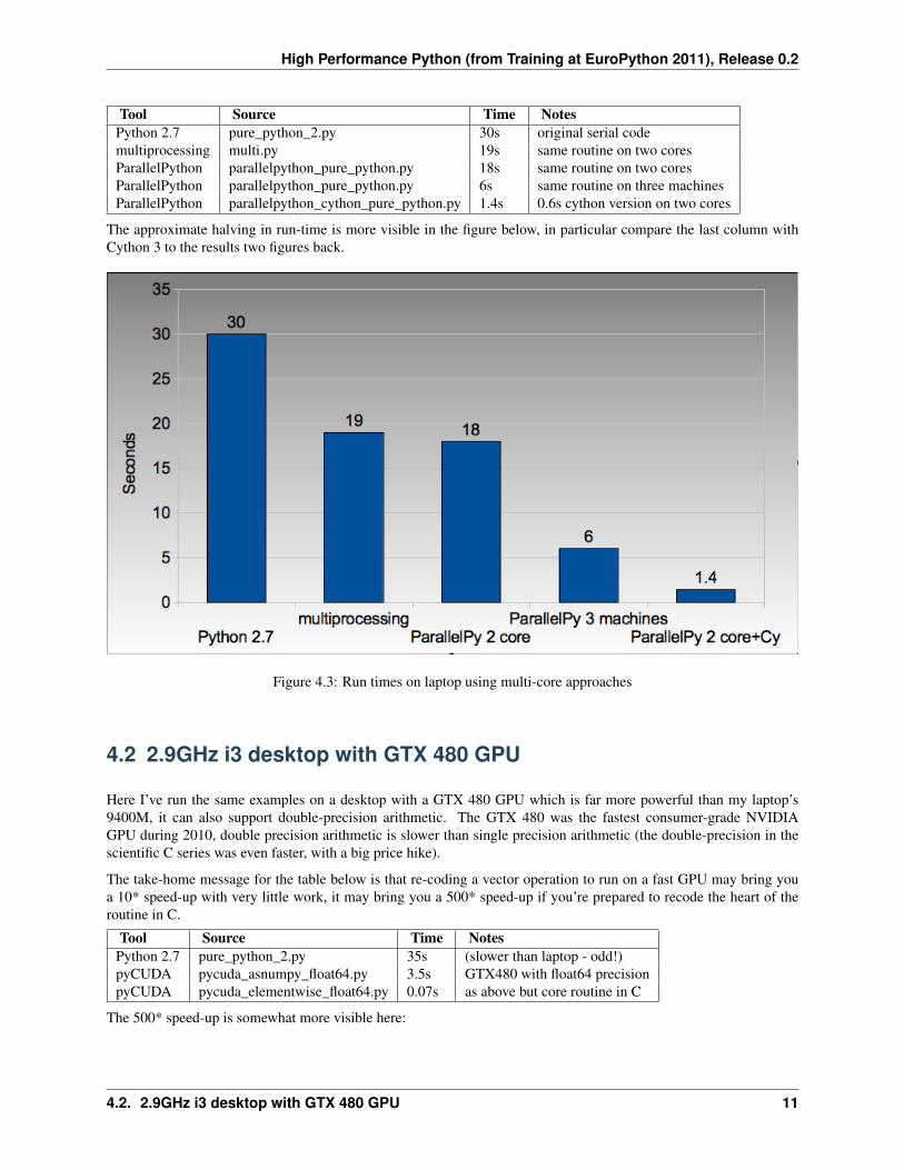
Tool Source Time NotesPython 2.7 pure_python_2.py 30s original serial codemultiprocessing multi.py 19s same routine on two coresParallelPython parallelpython_pure_python.py 18s same routine on two coresParallelPython parallelpython_pure_python.py 6s same routine on three machinesParallelPython parallelpython_cython_pure_python.py 1.4s 0.6s cython version on two cores

The approximate halving in run-time is more visible in the figure below, in particular compare the last column withCython 3 to the results two figures back.

Figure 4.3: Run times on laptop using multi-core approaches

4.2 2.9GHz i3 desktop with GTX 480 GPU

Here I’ve run the same examples on a desktop with a GTX 480 GPU which is far more powerful than my laptop’s9400M, it can also support double-precision arithmetic. The GTX 480 was the fastest consumer-grade NVIDIAGPU during 2010, double precision arithmetic is slower than single precision arithmetic (the double-precision in thescientific C series was even faster, with a big price hike).

The take-home message for the table below is that re-coding a vector operation to run on a fast GPU may bring youa 10* speed-up with very little work, it may bring you a 500* speed-up if you’re prepared to recode the heart of theroutine in C.

Tool Source Time NotesPython 2.7 pure_python_2.py 35s (slower than laptop - odd!)pyCUDA pycuda_asnumpy_float64.py 3.5s GTX480 with float64 precisionpyCUDA pycuda_elementwise_float64.py 0.07s as above but core routine in C

The 500* speed-up is somewhat more visible here:

4.2. 2.9GHz i3 desktop with GTX 480 GPU 11

High Performance Python (from Training at EuroPython 2011), Release 0.2

Figure 4.4: Run times on i3 desktop with GTX 480 GPU

4.2. 2.9GHz i3 desktop with GTX 480 GPU 12

CHAPTER

FIVE

USING THIS AS A TUTORIAL

If you grab the source from https://github.com/ianozsvald/EuroPython2011_HighPerformanceComputing (or Googlefor “ianozsvald github”) you can follow along. The github repository has the full source for all these examples (and afew others), you can start with the pure_python.py example and make code changes yourself.

You probably want to use numpy_loop.py and numpy_vector.py for the basis of some of the numpy transfor-mations.

13

CHAPTER

SIX

VERSIONS AND DEPENDENCIES

The tools depend on a few other libraries, you’ll want to install them first:

• CPython 2.7.2

• line_profiler 1.0b2

• RunSnake 2.0.1 (and it depends on wxPython)

• PIL (for drawing the plot)

• PyPy pypy-c-jit-45137-65b1ed60d7da-osx64 (from the nightly builds around July 2011)

• Cython 0.14.1

• Numpy 1.5.1

• ShedSkin 0.8 (and this depends on a few C libraries)

• NumExpr 1.4.2

• pyCUDA 0.94 (HEAD as of June 2011 and it depends on the CUDA development libraries, I’m using CUDA4.0)

14

CHAPTER

SEVEN

PURE PYTHON (CPYTHON)IMPLEMENTATION

Below we have the basic pure-python implementation. Typically you’ll be using CPython to run the code (CPythonbeing the Python language running in a C-language interpreter). This is the most common way to run Python code (onWindows you use python.exe, on Linux and Mac it is often just python).

In each example we have a calculate_z function (here it is calculate_z_serial_purepython), this doesthe hard work calculating the output vector which we’ll display. This is called by a calc function (in this case it iscalc_pure_python) which sets up the input and displays the output.

In calc I use a simple routine to prepare the x and y co-ordinates which is compatible between all the techniqueswe’re using. These co-ordinates are appended to the array q as complex numbers. We also initialise z as an arrayof the same length using complex(0,0). The motivation here is to setup some input data that is non-trivial whichmight match your own input in a real-world problem.

For my examples I used a 500 by 500 pixel plot with 1000 maximum iterations. Setting w and h to 1000 and usingthe default x1, x2, y1, y2 space we have a 500 by 500 pixel space that needs to be calculated. This means that zand q are 250,000 elements in length. Using a complex datatype (16 bytes) we have a total of 16 bytes * 250,000items * 2 arrays == 8,000,000 bytes (i.e. roughly 8MB of input data).

In the pure Python implementation on a core 2 duo MacBook using CPython 2.7.2 it takes roughly 52 seconds to solvethis task. We run it using:

>> python pure_python.py 1000 1000

If you have PIL and numpy installed then you’ll get the graphical plot.

NOTE that the first argument is 1000 and this results in a 500 by 500 pixel plot. This is confusing (and is based oninherited code that I should have fixed...) - I’ll fix the *2 oddness in a future version of this document. For now I’mmore interested in writing this up before I’m back from EuroPython!

# \python\pure_python.pyimport sysimport datetime# area of space to investigatex1, x2, y1, y2 = -2.13, 0.77, -1.3, 1.3

# Original code, prints progress (because it is slow)# Uses complex datatype

def calculate_z_serial_purepython(q, maxiter, z):"""Pure python with complex datatype, iterating over list of q and z"""output = [0] * len(q)for i in range(len(q)):

15

High Performance Python (from Training at EuroPython 2011), Release 0.2

if i % 1000 == 0:# print out some progress info since it is so slow...print "%0.2f%% complete" % (1.0/len(q) * i * 100)

for iteration in range(maxiter):z[i] = z[i]*z[i] + q[i]if abs(z[i]) > 2.0:

output[i] = iterationbreak

return output

def calc_pure_python(show_output):# make a list of x and y values which will represent q# xx and yy are the co-ordinates, for the default configuration they’ll look like:# if we have a 500x500 plot# xx = [-2.13, -2.1242, -2.1184000000000003, ..., 0.7526000000000064, 0.7584000000000064, 0.7642000000000064]# yy = [1.3, 1.2948, 1.2895999999999999, ..., -1.2844000000000058, -1.2896000000000059, -1.294800000000006]x_step = (float(x2 - x1) / float(w)) * 2y_step = (float(y1 - y2) / float(h)) * 2x=[]y=[]ycoord = y2while ycoord > y1:

y.append(ycoord)ycoord += y_step

xcoord = x1while xcoord < x2:

x.append(xcoord)xcoord += x_step

q = []for ycoord in y:

for xcoord in x:q.append(complex(xcoord,ycoord))

z = [0+0j] * len(q)print "Total elements:", len(z)start_time = datetime.datetime.now()output = calculate_z_serial_purepython(q, maxiter, z)end_time = datetime.datetime.now()secs = end_time - start_timeprint "Main took", secs

validation_sum = sum(output)print "Total sum of elements (for validation):", validation_sum

if show_output:try:

import Imageimport numpy as nmoutput = nm.array(output)output = (output + (256*output) + (256**2)*output) * 8im = Image.new("RGB", (w/2, h/2))im.fromstring(output.tostring(), "raw", "RGBX", 0, -1)im.show()

except ImportError as err:# Bail gracefully if we’re using PyPyprint "Couldn’t import Image or numpy:", str(err)

if __name__ == "__main__":

16

High Performance Python (from Training at EuroPython 2011), Release 0.2

# get width, height and max iterations from cmd line# ’python mandelbrot_pypy.py 100 300’w = int(sys.argv[1]) # e.g. 100h = int(sys.argv[1]) # e.g. 100maxiter = int(sys.argv[2]) # e.g. 300

# we can show_output for Python, not for PyPycalc_pure_python(True)

When you run it you’ll also see a validation sum - this is the summation of all the values in the output list, ifthis is the same between executions then your program’s math is progressing in exactly the same way (if it is differentthen something different is happening!). This is very useful when you’re changing one form of the code into another -it should always produce the same validation sum.

17

CHAPTER

EIGHT

PROFILING WITH CPROFILE ANDLINE_PROFILER

The profile module is the standard way to profile Python code, take a look at it herehttp://docs.python.org/library/profile.html. We’ll run it on our simple Python implemen-tation:

>> python -m cProfile -o rep.prof pure_python.py 1000 1000

This generates a rep.prof output file containing the profiling results, we can now load this into the pstatsmoduleand print out the top 10 slowest functions:

>>> import pstats>>> p = pstats.Stats(’rep.prof’)>>> p.sort_stats(’cumulative’).print_stats(10)

Fri Jun 24 17:13:11 2011 rep.prof

51923594 function calls (51923523 primitive calls) in 54.333 seconds

Ordered by: cumulative timeList reduced from 558 to 10 due to restriction <10>

ncalls tottime percall cumtime percall filename:lineno(function)1 0.017 0.017 54.335 54.335 pure_python.py:1(<module>)1 0.268 0.268 54.318 54.318 pure_python.py:28(calc_pure_python)1 37.564 37.564 53.673 53.673 pure_python.py:10(calculate_z_serial_purepython)

51414419 12.131 0.000 12.131 0.000 {abs}250069 3.978 0.000 3.978 0.000 {range}

1 0.005 0.005 0.172 0.172 .../numpy/__init__.py:106(<module>)1 0.001 0.001 0.129 0.129 .../numpy/add_newdocs.py:9(<module>)1 0.004 0.004 0.116 0.116 .../numpy/lib/__init__.py:1(<module>)1 0.001 0.001 0.071 0.071 .../numpy/lib/type_check.py:3(<module>)1 0.013 0.013 0.070 0.070 .../numpy/core/__init__.py:2(<module>)

Take a look at the profile module’s Python page for details. Basically the above tells us thatcalculate_z_serial_purepython is run once, costs 37 seconds for its own lines of code and in total (in-cluding the other functions it calls) costs a total of 53 seconds. This is obviously our bottleneck.

We can also see that abs is called 51,414,419 times, each call costs a tiny fraction of a second but 54 million add upto 12 seconds.

The final lines of the profile relate to numpy - this is the numerical library I’ve used to convert the Python lists into aPIL-compatible RGB string for visualisation (so you need PIL and numpy installed).

18

High Performance Python (from Training at EuroPython 2011), Release 0.2

For more complex programs the output becomes hard to understand. runsnake is a great tool to visualise the profiledresults:

>> runsnake rep.prof

This generates a display like:

Figure 8.1: RunSnakeRun’s output on pure_python.py

Now we can visually see where the time is spent. I use this to identify which functions are worth dealing with first ofall - this tool really comes into its own when you have a complex project with many modules.

However - which lines are causing our code to run slow? This is the more interesting question and cProfile can’tanswer it.

Let’s look at the line_profer module. First we have to decorate our chosen function with @profile:

@profiledef calculate_z_serial_purepython(q, maxiter, z):

Next we’ll run kernprof.py and ask it to do line-by-line profiling and to give us a visual output, then we tell itwhat to profile. Note that we’re running a much smaller problem as line-by-line profiling takes ages:

>> kernprof.py -l -v pure_python.py 300 100

File: pure_python.pyFunction: calculate_z_serial_purepython at line 9Total time: 354.689 s

Line # Hits Time Per Hit % Time Line Contents==============================================================

9 @profile10 def calculate_z_serial_purepython(q, maxiter, z):

19

High Performance Python (from Training at EuroPython 2011), Release 0.2

11 """Pure python with complex datatype, iterating over list of q and z"""12 1 2148 2148.0 0.0 output = [0] * len(q)13 250001 534376 2.1 0.2 for i in range(len(q)):14 250000 550484 2.2 0.2 if i % 1000 == 0:15 # print out some progress info since it is so slow...16 250 27437 109.7 0.0 print "%0.2f%% complete" % (1.0/len(q) * i * 100)17 51464485 101906246 2.0 28.7 for iteration in range(maxiter):18 51414419 131859660 2.6 37.2 z[i] = z[i]*z[i] + q[i]19 51414419 116852418 2.3 32.9 if abs(z[i]) > 2.0:20 199934 429692 2.1 0.1 output[i] = iteration21 199934 2526311 12.6 0.7 break22 1 9 9.0 0.0 return output

Here we can see that the bulk of the time is spent in the for iteration in range(maxiter): loop. If thez[i] = z[i] * z[i] + q[i] and if abs(z[i]) > 2.0: lines ran faster then the entire function wouldrun much faster.

This is the easiest way to identify which lines are causing you the biggest problems. Now you can focus on fixing thebottleneck rather than guessing at which lines might be slow!

REMEMBER to remove the @profile decorator when you’re done with kernprof.py else Python will throwan exception (it won’t recognise @profile outside of kernprof.py).

As a side note - the profiling approaches shown here work well for non-CPU bound tasks too. I’ve successfully profileda bottle.py web server, it helps to identify anywhere where things are running slowly (e.g. slow file access or toomany SQL statements).

20

CHAPTER

NINE

BYTECODE ANALYSIS

There are several keys ways that you can make your code run faster. Having an understanding of what’s happening inthe background can be useful. Python’s dis module lets us disassemble the code to see the underlying bytecode.

We can use dis.dis(fn) to disassemble the bytecode which represents fn. First we’ll import pure_pythonto bring our module into the namespace:

>>> import pure_python # imports our solver into Python>>> dis.dis(pure_python.calculate_z_serial_purepython)....18 109 LOAD_FAST 2 (z) # load z

112 LOAD_FAST 4 (i) # load i115 BINARY_SUBSCR # get value in z[i]116 LOAD_FAST 2 (z) # load z119 LOAD_FAST 4 (i) # load i122 BINARY_SUBSCR # get value in z[i]123 BINARY_MULTIPLY # z[i] * z[i]124 LOAD_FAST 0 (q) # load z127 LOAD_FAST 4 (i) # load i130 BINARY_SUBSCR # get q[i]131 BINARY_ADD # add q[i] to last multiply132 LOAD_FAST 2 (z) # load z135 LOAD_FAST 4 (i) # load i138 STORE_SUBSCR # store result in z[i]

19 139 LOAD_GLOBAL 2 (abs) # load abs function142 LOAD_FAST 2 (z) # load z145 LOAD_FAST 4 (i) # load i148 BINARY_SUBSCR # get z[i]149 CALL_FUNCTION 1 # call abs152 LOAD_CONST 6 (2.0) # load 2.0155 COMPARE_OP 4 (>) # compare result of abs with 2.0158 POP_JUMP_IF_FALSE 103 # jump depending on result

...

Above we’re looking at lines 18 and 19. The right column shows the operations with my annotations. You can see thatwe load z and i onto the stack a lot of times.

Pragmatically you won’t optimise your code by using the dis module but it does help to have an understanding ofwhat’s going on under the bonnet.

21

CHAPTER

TEN

A (SLIGHTLY) FASTER CPYTHONIMPLEMENTATION

Having taken a look at bytecode, let’s make a small modification to the code. This modification is only necessary forCPython and PyPy - the C compiler options for us won’t need the modification.

All we’ll do is dereference the z[i] and q[i] calls once, rather than many times in the inner loops:

# \python\pure_python_2.pyfor i in range(len(q)):

zi = z[i]qi = q[i]...for iteration in range(maxiter):

zi = zi * zi + qiif abs(zi) > 2.0:

Now look at the kernprof.py output on our modified pure_python_2.py. We have the same number offunction calls but they’re quicker - the big change being the cost of 2.6 seconds dropping to 2.2 seconds for the z =z * z + q line. If you’re curious about how the change is reflected in the underlying bytecode then I urge that youtry the dis module on your modified code.

File: pure_python_2.pyFunction: calculate_z_serial_purepython at line 10Total time: 327.168 s

Line # Hits Time Per Hit % Time Line Contents==============================================================

10 @profile11 def calculate_z_serial_purepython(q, maxiter, z):12 """Pure python with complex datatype, iterating over list of q and z"""13 1 2041 2041.0 0.0 output = [0] * len(q)14 250001 519749 2.1 0.2 for i in range(len(q)):15 250000 508612 2.0 0.2 zi = z[i]16 250000 511306 2.0 0.2 qi = q[i]17 250000 535007 2.1 0.2 if i % 1000 == 0:18 # print out some progress info since it is so slow...19 250 26760 107.0 0.0 print "%0.2f%% complete" % (1.0/len(q) * i * 100)20 51464485 100041485 1.9 30.6 for iteration in range(maxiter):21 51414419 112112069 2.2 34.3 zi = zi * zi + qi22 51414419 109947201 2.1 33.6 if abs(zi) > 2.0:23 199934 419932 2.1 0.1 output[i] = iteration24 199934 2543678 12.7 0.8 break25 1 9 9.0 0.0 return output

22

High Performance Python (from Training at EuroPython 2011), Release 0.2

Here’s the improved bytecode:

>>> dis.dis(calculate_z_serial_purepython)...22 129 LOAD_FAST 5 (zi)

132 LOAD_FAST 5 (zi)135 BINARY_MULTIPLY136 LOAD_FAST 6 (qi)139 BINARY_ADD140 STORE_FAST 5 (zi)

24 143 LOAD_GLOBAL 2 (abs)146 LOAD_FAST 5 (zi)149 CALL_FUNCTION 1152 LOAD_CONST 6 (2.0)155 COMPARE_OP 4 (>)158 POP_JUMP_IF_FALSE 123

...

You can see that we don’t have to keep loading z and i, so we execute fewer instructions (so things run faster).

23

CHAPTER

ELEVEN

PYPY

PyPy is a new Just In Time compiler for the Python programming language. It runs on Windows, Mac and Linux andas of the middle of 2011 it runs Python 2.7. Generally you code will just run in PyPy and often it’ll run faster (I’veseen reports of 2-10* speed-ups). Sometimes small amounts of work are required to correct code that runs in CPythonbut shows errors in PyPy. Generally this is because the programmer has (probably unwittingly!) used shortcuts thatwork in CPython that aren’t actually correct in the Python specification.

Our example runs without modification in PyPy. I’ve used both PyPy 1.5 and the latest HEAD from the nightly builds(taken on June 20th for my Mac). The latest nightly build is a bit faster than PyPy 1.5, I’ve used the timings from thenightly build here.

If you aren’t using a C library like numpy then you should try PyPy - it might just make your code run several timesfaster. At EuroPython 2011 I saw a Sobel Edge Detection demo than runs in pure Python - with PyPy it runs 450*faster than CPython! The PyPy team are committed to making PyPy faster and more stable, since it supports Python2.7 (which is the end of the Python 2.x line) you can expect it to keep getting faster for a while yet.

If you use a C extension like numpy then expect problems - some C libraries are integrated, many aren’t, some likenumpy will probably require a re-write (which will be a multi-month undertaking). During 2011 at least it looks asthough numpy integration will not happen. Note that you can do import numpy in pypy and you’ll get a minimalarray interface that behaves in a numpy-like fashion but for now it has very few functions and only supports doublearithmetic.

By running pypy pure_python.py 1000 1000 on my MacBook it takes 5.9 seconds, running pypypure_python_2.py 1000 1000 it takes 4.9 seconds. Note that there’s no graphical output - PIL is supported inPyPy but numpy isn’t and I’ve used numpy to generate the list-to-RGB-array conversion (update see the last sectionof this document for a fix that removes numpy and allows PIL to work with PyPy!).

As an additional test (not shown in the graphs) I ran pypy shedskin2.py 1000 1000 which runs the expandedmath version of the shedskin variant below (this replaces complex numbers with floats and expands abs toavoid the square root). The shedskin2.py result takes 3.2 seconds (which is still much slower than the 0.4s versioncompiled using shedskin).

11.1 numpy

Work has started to add a new numpy module to PyPy. Currently (July 2011) it only supports arrays of doubleprecision numbers and offers very few vectorised functions:

Python 2.7.1 (65b1ed60d7da, Jul 12 2011, 02:00:13)[PyPy 1.5.0-alpha0 with GCC 4.0.1] on darwinType "help", "copyright", "credits" or "license" for more information.And now for something completely different: ‘‘2008 will be the year of thedesktop on #pypy’’

24

High Performance Python (from Training at EuroPython 2011), Release 0.2

>>>> import numpy>>>> dir(numpy)[’__doc__’, ’__file__’, ’__name__’, ’__package__’, ’abs’, ’absolute’, ’array’, ’average’,’copysign’, ’empty’, ’exp’, ’floor’, ’maximum’, ’mean’, ’minimum’, ’negative’, ’ones’,’reciprocal’, ’sign’, ’zeros’]

>>>> a = numpy.array(range(10))>>>> [x for x in a] # print the contents of a[0.0, 1.0, 2.0, 3.0, 4.0, 5.0, 6.0, 7.0, 8.0, 9.0]>>>>>>>> [x for x in a+3] # perform a vectorised addition on a[3.0, 4.0, 5.0, 6.0, 7.0, 8.0, 9.0, 10.0, 11.0, 12.0]

It would be possible to rewrite the Mandelbrot example using these functions by using non-complex arithmetic (seee.g. the shedskin2.py example later). This is a challenge I’ll leave to the reader.

I strongly urge you to join the PyPy mailing list and talk about your needs for the new numpy library. PyPy showsgreat promise for high performance Python with little effort, having access to the wide range of algorithms in theexisting numpy library would be a massive boon to the community.

11.1. numpy 25

CHAPTER

TWELVE

PSYCO

Psyco is a Just In Time compiler for 32 bit Python, it used to be really popular but it is less supported on Python 2.7and doesn’t (and won’t) run on 64 bit systems. The author now works exclusively on PyPy.

IAN_TODO consider running pure_python/pure_python_2/shedskin2 on Ubuntu 32 bit with Python 2.6 32 bit

26

CHAPTER

THIRTEEN

CYTHON

Cython lets us annotate our functions so they can be compiled to C. It takes a little bit of work (30-60 minutes to getstarted) and then typically gives us a nice speed-up. If you’re new to Cython then the official tutorial is very helpful:http://docs.cython.org/src/userguide/tutorial.html

To start this example I’ll assume you’ve moved pure_python_2.py into a new directory (e.g.cython_pure_python\cython_pure_python.py). We’ll start a new module called calculate_z.py,move the calculate_z function into this module. In cython_pure_python.py you’ll have to importcalculate_z and replace the reference to calculate_z(...) with calculate_z.calculate_z(...).

Verify that the above runs. The contents of your calculate_z.py will look like:

# calculate_z.py# based on calculate_z_serial_purepythondef calculate_z(q, maxiter, z):

output = [0] * len(q)for i in range(len(q)):

zi = z[i]qi = q[i]for iteration in range(maxiter):

zi = zi * zi + qiif abs(zi) > 2.0:

output[i] = iterationbreak

return output

Now rename calculate_z.py to calculate_z.pyx, Cython uses .pyx (based on the older Pyrex project) toindicate a file that it’ll compile to C.

Now add a new setup.py with the following contents:

# setup.pyfrom distutils.core import setupfrom distutils.extension import Extensionfrom Cython.Distutils import build_ext

# for notes on compiler flags see:# http://docs.python.org/install/index.html

setup(cmdclass = {’build_ext’: build_ext},ext_modules = [Extension("calculate_z", ["calculate_z.pyx"])])

Next run:

27

High Performance Python (from Training at EuroPython 2011), Release 0.2

>> python setup.py build_ext --inplace

This runs our setup.py script, calling the build_ext command. Our new module is built in-place in our directory,you should end up with a new calculate_z.so in this directory.

Run the new code using python cython_pure_python.py 1000 1000 and confirm that the result is calcu-lated more quickly (you may find that the improvement is very minor at this point!).

You can take a look to see how well the slower Python calls are being replaced with faster Cython calls using:

>> cython -a calculate_z.pyx

This will generate a new .html file, open that in your browser and you’ll see something like:

Figure 13.1: Result of “cython -a calculate_z.pyx” in web browser

Each time you add a type annotation Cython has the option to improve the resulting code. When it does so successfullyyou’ll see the dark yellow lines turn lighter and eventually they’ll turn white (showing that no further improvement ispossible).

If you’re curious, double click a line of yellow code and it’ll expand to show you the C Python API calls that it ismaking (see the figure).

Let’s add the annotations, see the example below where I’ve added type definitions. Remember to run the cython-a ... command and monitor the reduction in yellow in your web browser.

# based on calculate_z_serial_purepythondef calculate_z(list q, int maxiter, list z):

cdef unsigned int icdef int iterationcdef complex zi, qi # if you get errors here try ’cdef complex double zi, qi’cdef list output

output = [0] * len(q)for i in range(len(q)):

28

High Performance Python (from Training at EuroPython 2011), Release 0.2

Figure 13.2: Double click a line to show the underlying C API calls (more calls mean more yellow)

29

High Performance Python (from Training at EuroPython 2011), Release 0.2

zi = z[i]qi = q[i]for iteration in range(maxiter):

zi = zi * zi + qiif abs(zi) > 2.0:

output[i] = iterationbreak

return output

Recompile using the setup.py line above and confirm that the result is much faster!

As you’ll see in the ShedSkin version below we can achieve the best speed-up by expanding the complicated complexobject into simpler double precision floating point numbers. The underlying C compiler knows how to execute theseinstructions in a faster way.

Expanding complexmultiplication and addition involves a little bit of algebra (see WikiPedia for details). We declarea set of intermediate variables cdef double zx, zy, qx, qy, zx_new, zy_new, dereference them fromz[i] and q[i] and then replaced the final abs call with the expanded if (zx*zx + zy*zy) > 4.0 logic (thesqrt of 4 is 2.0, abs would otherwise perform an expensive square-root on the result of the addition of the squares).

# calculate_z.pyx_2_bettermathdef calculate_z(list q, int maxiter, list z):

cdef unsigned int icdef int iterationcdef list outputcdef double zx, zy, qx, qy, zx_new, zy_new

output = [0] * len(q)for i in range(len(q)):

zx = z[i].real # need to extract items using dot notationzy = z[i].imagqx = q[i].realqy = q[i].imag

for iteration in range(maxiter):zx_new = (zx * zx - zy * zy) + qxzy_new = (zx * zy + zy * zx) + qy# must assign after else we’re using the new zx/zy in the flazx = zx_newzy = zy_new# note - math.sqrt makes this almost twice as slow!#if math.sqrt(zx*zx + zy*zy) > 2.0:if (zx*zx + zy*zy) > 4.0:

output[i] = iterationbreak

return output

13.1 Compiler directives

Cython has several compiler directives that enable profiling with cProfile and can improve performance:http://wiki.cython.org/enhancements/compilerdirectives

The directives can be enabled globally (in the Cython) file using a comment at the top of the file or by alteringsetup.py and you can decorate each function individually. Generally I only have a few functions in a .pyx file soI enable the directives globally in the module using the comment syntax.

13.1. Compiler directives 30

High Performance Python (from Training at EuroPython 2011), Release 0.2

profile lets you enable or disable cProfile support. This is only useful when profiling (and adds a minoroverhead). It gives you exactly the same output as running cProfile on a normal Python module.

boundscheck lets you disable out-of-bounds index checking on buffered arrays (mostly this will apply to numpyarrays - see next section). Since it doesn’t need to check for IndexError exceptions it runs faster. If you makea mistake here then expect a segmentation fault. I have seen speed-ups using this option but not for the Mandelbrotproblem shown here.

wraparound can disable support for -n array indexing (i.e. indexing backwards). In my experiments I’ve not seenthis option generate a speed-up.

There is also experimental infer_types support which is supposed to guess the type of variables, I’ve not achievedany speed-up when trying this (unlike for ShedSkin where the automatic type inference works wonderfully well).

13.2 prange

In the upcoming release of Cython (v0.15 - expected after July 2011) we should see the introduction of the prangeconstruct: http://wiki.cython.org/enhancements/prange

This wraps the OpenMP parallel for directive so multiple cores can operate on a container at the same time.This should work well for the Mandelbrot example here.

13.2. prange 31

CHAPTER

FOURTEEN

CYTHON WITH NUMPY ARRAYS

Below we have a similar Cython file, the original version for this approach was subbmited by Didrik Pinteof Enthought (thanks Didrik!). The main difference is the annotation of numpy arrays, see the tutorial fora great walkthrough: http://docs.cython.org/src/tutorial/numpy.html (and there’s a bit more detail in the wiki:http://wiki.cython.org/tutorials/numpy).

Using the numpy approach Python is able to address the underlying C data structures that are wrapped by numpywithout the Python call overheads. This version of the Mandelbrot solver runs almost at the same speed as the ShedSkinsolution (shown in the next section), making it the second fastest single-CPU implementation in this tutorial.

IAN_TODO I ought to remove Didrik’s local declaration of z = 0+0j to make it a fairer comparision with therest of the code (though my gut says that this will have little effect on the runtime)

# calculate_z.pyx# see ./cython_numpy_loop/cython_numpy_loop.pyfrom numpy import empty, zeroscimport numpy as np

def calculate_z(np.ndarray[double, ndim=1] xs, np.ndarray[double, ndim=1] ys, int maxiter):""" Generate a mandelbrot set """cdef unsigned int i,jcdef unsigned int N = len(xs)cdef unsigned int M = len(ys)cdef double complex qcdef double complex zcdef int iteration

cdef np.ndarray[int, ndim=2] d = empty(dtype=’i’, shape=(M, N))for j in range(M):

for i in range(N):# create q without intermediate object (faster)q = xs[i] + ys[j]*1jz = 0+0jfor iteration in range(maxiter):

z = z*z + qif z.real*z.real + z.imag*z.imag > 4.0:

breakelse:

iteration = 0d[j,i] = iteration

return d

32

CHAPTER

FIFTEEN

SHEDSKIN

ShedSkin automatically annotates your Python module and compiles it down to C. It works in a more restricted setof circumstances than Cython but when it works - it Just Works and requires very little effort on your part. One ofthe included examples is a Commodore 64 emulator that jumps from a few frames per second with CPython whendemoing a game to over 50 FPS, where the main emulation is compiled by ShedSkin and used as an extension moduleto pyGTK running in CPython.

Its main limitations are:

• prefers short modules (less than 3,000 lines of code - this is still rather a lot for a bottleneck routine!)

• only uses built-in modules (e.g. you can’t import numpy or PIL into a ShedSkin module)

The release announce for v0.8 includes a scalability graph http://shed-skin.blogspot.com/2011/06/shed-skin-08-programming-language.html showing compile times for longer Python modules. It can output either a compiledexecutable or an importable module.

You run it using shedskin your_module.py. In our case move pure_python_2.py into a new directory(shedskin_pure_python\shedskin_pure_python.py). We could make a new module (as we did for theCython example) but for now we’ll just one the one Python file.

Run:

shedskin shedskin_pure_python.pymake

After this you’ll have shedskin_pure_python which is an executable. Try it and see what sort of speed-up youget.

ShedSkin has local C implementations of all of the core Python library (it can only import C-implemented modulesthat someone has written for ShedSkin!). For this reason we can’t use numpy in a ShedSkin executable or module,you can pass a Python list across (and numpy lets you make a Python list from an array type), but that comeswith a speed hit.

The complex datatype has been implemented in a way that isn’t as efficient as it could be (ShedSkin’s author MarkDufour has stated that it could be made much more efficient if there’s demand). If we expand the math using somealgebra in exactly the same way that we did for the Cython example we get another huge jump in performance:

def calculate_z_serial_purepython(q, maxiter, z):output = [0] * len(q)for i in range(len(q)):

zx, zy = z[i].real, z[i].imagqx, qy = q[i].real, q[i].imagfor iteration in range(maxiter):

# expand complex numbers to floats, do raw float arithmetic# as the shedskin variant isn’t so fast# I believe MD said that complex numbers are allocated on the heap

33

High Performance Python (from Training at EuroPython 2011), Release 0.2

# and this could easily be improved for the next shedskinzx_new = (zx * zx - zy * zy) + qxzy_new = (2 * (zx * zy)) + qy # note that zx(old) is used so we make zx_new on previous linezx = zx_newzy = zy_new# remove need for abs and just square the numbersif zx*zx + zy*zy > 4.0:

output[i] = iterationbreak

return output

When debugging it is helpful to know what types the code analysis has detected. Use:

shedskin -a your_module.py

and you’ll have annotated .cpp and .hpp files which tie the generated C with the original Python.

15.1 Profiling

I’ve never tried profiling ShedSkin but several options (using ValGrind and GProf) were presented in the GoogleGroup: http://groups.google.com/group/shedskin-discuss/browse_thread/thread/fd39b6bb38cfb6d1

15.2 Faster code

You can disable bounds-checking with the -b flag, generally this gives a small speed improvement. Wrap-aroundchecking can be disabled with -w. Neither optimisation improved the run-time for this problem. For int64 longinteger support add -l. For other flags see the documentation.

The author made some notes in the ShedSkin Google Group http://groups.google.com/group/shedskin-discuss/browse_thread/thread/c5bf965a80292a43 on speeding up the code by editing the generated Makefile:

• adding -ffast-math to FLAGS seems to reduce run-time by about 10%

• compiling first with -fprofile-generate then -fprofile-use saves about 7%

• using libgc 7.2alpha6 instead of the common libgc 6.8 helps about 3% (you may already use thisone)

It is possible that automatic vectorisation (e.g. with gcc http://gcc.gnu.org/projects/tree-ssa/vectorization.html) willhelp, I don’t have an up to date gcc (e.g. 4.6) on my MacBook so I’ve yet to experiment with this.

15.1. Profiling 34

CHAPTER

SIXTEEN

NUMPY VECTORS

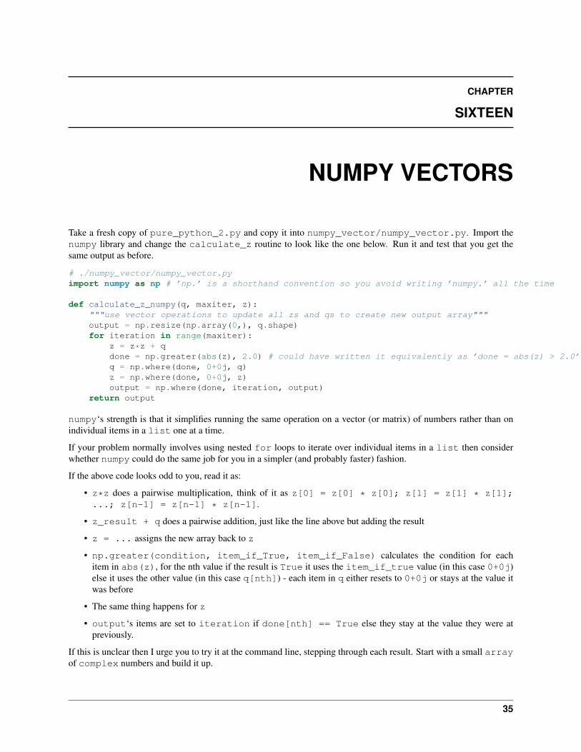
Take a fresh copy of pure_python_2.py and copy it into numpy_vector/numpy_vector.py. Import thenumpy library and change the calculate_z routine to look like the one below. Run it and test that you get thesame output as before.

# ./numpy_vector/numpy_vector.pyimport numpy as np # ’np.’ is a shorthand convention so you avoid writing ’numpy.’ all the time

def calculate_z_numpy(q, maxiter, z):"""use vector operations to update all zs and qs to create new output array"""output = np.resize(np.array(0,), q.shape)for iteration in range(maxiter):

z = z*z + qdone = np.greater(abs(z), 2.0) # could have written it equivalently as ’done = abs(z) > 2.0’q = np.where(done, 0+0j, q)z = np.where(done, 0+0j, z)output = np.where(done, iteration, output)

return output

numpy‘s strength is that it simplifies running the same operation on a vector (or matrix) of numbers rather than onindividual items in a list one at a time.

If your problem normally involves using nested for loops to iterate over individual items in a list then considerwhether numpy could do the same job for you in a simpler (and probably faster) fashion.

If the above code looks odd to you, read it as:

• z*z does a pairwise multiplication, think of it as z[0] = z[0] * z[0]; z[1] = z[1] * z[1];...; z[n-1] = z[n-1] * z[n-1].

• z_result + q does a pairwise addition, just like the line above but adding the result

• z = ... assigns the new array back to z

• np.greater(condition, item_if_True, item_if_False) calculates the condition for eachitem in abs(z), for the nth value if the result is True it uses the item_if_true value (in this case 0+0j)else it uses the other value (in this case q[nth]) - each item in q either resets to 0+0j or stays at the value itwas before

• The same thing happens for z

• output‘s items are set to iteration if done[nth] == True else they stay at the value they were atpreviously.

If this is unclear then I urge you to try it at the command line, stepping through each result. Start with a small arrayof complex numbers and build it up.

35

High Performance Python (from Training at EuroPython 2011), Release 0.2

You’ll probably be curious why this code runs slower than the other numpy version that uses Cython. The reason isthat the vectorised code can’t stop early on each iteration if output has been set - it has to do the same operationsfor all items in the array. This is a shortcoming of this example. Don’t be put off by vectors, normally you can’t exitloops early (particuarly in the physics problems I tend to work on).

Behind the scenes numpy is using very fast C optimised math libraries to perform these calculations very quickly.If you consider how much extra work it is having to do (since it can’t exit each calculation loop when output iscalculated for a co-ordinate) it is amazing that it is still going so fast!

36

CHAPTER

SEVENTEEN

NUMPY VECTORS AND CACHECONSIDERATIONS

The following figure refers to numpy_vector_2.py where I vary the vector size that I’m dealing with by takingslices out of each numpy vector. We can see that the run time on the laptop (blue) and i3 desktop (orange) hits a sweetspot around an array length of 20,000 items.

Oddly this represents a total of about 640k of data between the two arrays, way below the 3MB L2 cache on both ofmy machines.

Figure 17.1: Array and cache size considerations

The code I’ve used looks like:

def calculate_z_numpy(q_full, maxiter, z_full):output = np.resize(np.array(0,), q_full.shape)#STEP_SIZE = len(q_full) # 54s for 250,000#STEP_SIZE = 90000 # 52#STEP_SIZE = 50000 # 45s

37

High Performance Python (from Training at EuroPython 2011), Release 0.2

#STEP_SIZE = 45000 # 45sSTEP_SIZE = 20000 # 42s # roughly this looks optimal on Macbook and dual core desktop i3#STEP_SIZE = 10000 # 43s#STEP_SIZE = 5000 # 45s#STEP_SIZE = 1000 # 1min02#STEP_SIZE = 100 # 3minsprint "STEP_SIZE", STEP_SIZEfor step in range(0, len(q_full), STEP_SIZE):

z = z_full[step:step+STEP_SIZE]q = q_full[step:step+STEP_SIZE]for iteration in range(maxiter):

z = z*z + qdone = np.greater(abs(z), 2.0)q = np.where(done,0+0j, q)z = np.where(done,0+0j, z)output[step:step+STEP_SIZE] = np.where(done, iteration, output[step:step+STEP_SIZE])

return output

38

CHAPTER

EIGHTEEN

NUMEXPR ON NUMPY VECTORS

numexpr is a wonderfully simple library - you wrap your numpy expression in numexpr.evaluate(<yourcode>) and often it’ll simply run faster! In the example below I’ve commented out the numpy vector code from thesection above and replaced it with the numexpr variant:

import numexpr...def calculate_z_numpy(q, maxiter, z):

output = np.resize(np.array(0,), q.shape)for iteration in range(maxiter):

#z = z*z + qz = numexpr.evaluate("z*z+q")#done = np.greater(abs(z), 2.0)done = numexpr.evaluate("abs(z).real > 2.0")#q = np.where(done,0+0j, q)q = numexpr.evaluate("where(done, 0+0j, q)")#z = np.where(done,0+0j, z)z = numexpr.evaluate("where(done, 0+0j, z)")#output = np.where(done, iteration, output)output = numexpr.evaluate("where(done, iteration, output)")

return output

I’ve replaced np.greater with >, the use of np.greater just showed another way of achieving the same taskearlier (but numexpr doesn’t let us refer to numpy functions, just the functions it provides).

You can only use numexpr on numpy code and it only makes sense to use it on vector operations. In the backgroundnumexpr breaks operations down into smaller segments that will fit into the CPU’s cache, it’ll also auto-vectoriseacross the available math units on the CPU if possible.

On my dual-core MacBook I see a 2-3* speed-up. If I had an Intel MKL version of numexpr (warning - needs acommercial license from Intel or Enthought) then I might see an even greater speed-up.

numexpr can give us some useful system information:

>>> numexpr.print_versions()-=-=-=-=-=-=-=-=-=-=-=-=-=-=-=-=-=-=-=-=-=-=-=-=-=-=-=-=-=-=-=-=-=-=-=-=-=-=Numexpr version: 1.4.2NumPy version: 1.5.1Python version: 2.7.1 (r271:86882M, Nov 30 2010, 09:39:13)[GCC 4.0.1 (Apple Inc. build 5494)]Platform: darwin-i386AMD/Intel CPU? FalseVML available? FalseDetected cores: 2-=-=-=-=-=-=-=-=-=-=-=-=-=-=-=-=-=-=-=-=-=-=-=-=-=-=-=-=-=-=-=-=-=-=-=-=-=-=

39

High Performance Python (from Training at EuroPython 2011), Release 0.2

It can also gives us some very low-level information about our CPU:

>>> numexpr.cpu.info{’arch’: ’i386’,’machine’: ’i486’,’sysctl_hw’: {’hw.availcpu’: ’2’,

’hw.busfrequency’: ’1064000000’,’hw.byteorder’: ’1234’,’hw.cachelinesize’: ’64’,’hw.cpufrequency’: ’2000000000’,’hw.epoch’: ’0’,’hw.l1dcachesize’: ’32768’,’hw.l1icachesize’: ’32768’,’hw.l2cachesize’: ’3145728’,’hw.l2settings’: ’1’,’hw.machine’: ’i386’,’hw.memsize’: ’4294967296’,’hw.model’: ’MacBook5,2’,’hw.ncpu’: ’2’,’hw.pagesize’: ’4096’,’hw.physmem’: ’2147483648’,’hw.tbfrequency’: ’1000000000’,’hw.usermem’: ’1841561600’,’hw.vectorunit’: ’1’}}

We can also use it to pre-compile expressions (so they don’t have to be compiled dynamically in each loop - this cansave time if you have a very fast loop) and then look as the disassembly (though I doubt you’d do anything with thedisassembled output):

>>> expr = numexpr.NumExpr(’avector > 2.0’) # pre-compile an expression>>> numexpr.disassemble(expr):[(’gt_bdd’, ’r0’, ’r1[output]’, ’c2[2.0]’)]>>> somenbrs = np.arange(10) # -> array([0, 1, 2, 3, 4, 5, 6, 7, 8, 9])>>> expr.run(somenbrs)array([False, False, False, True, True, True, True, True, True, True], dtype=bool)

You might choose to pre-compile an expression in a fast loop if the overhead of compiling (as reported bykernprof.py) reduces the benefit of the speed-ups achieved.

40

CHAPTER

NINETEEN

PYCUDA

Andreas Klöckner’s pyCUDA wraps NVIDIA’s C interface to their Compute Unified Device Architecture in a set offriendly Python API calls. A numpy-like interface is provided (slowest but easiest to use) along with an element-wiseinterface and a pure C code wrapper (both require you to write C code).

In this tutorial I’m using an older MacBook with an NVIDIA 9400M graphics card. This card only supports singleprecision floating point arithmetic, newer cards (e.g. the GTX 480 shown in the graph at the start of this tutorial)also support double precision floating point numbers as used in all the other examples here. As a result the fol-lowing examples show float32 and complex64 (comprising two float32 numbers) rather than float64 andcomplex128. You can swap the comments around if you have a newer card.

I would expect all future GPUs to support double precision arithmetic, possibly mobile phone GPUs will be limitedto single precision for a while yet though.

If you want an idea of what a high-spec GPU looks like - this is the GTX 480 in my desktop (note how it is largecompared to the motherboard!) at my physics client:

Figure 19.1: GTX 480 GPU (top of the line in 2010!)

You’ll have to spend some time getting your head around GPU programming. Vector operations are assumed (see thenumpy vector examples above) and the GPU has its own memory that’s separate from the CPU’s memory, so data has

41

High Performance Python (from Training at EuroPython 2011), Release 0.2

to be copied to the card before processing.

The copy operations incur a time overhead - remember that it takes time to copy data to the GPU, then time to run thecode (which is typically faster running in parallel on the GPU than in series on a CPU), then it takes time to copy theresult back. The overheads for the copying have to be less than the speed-up you obtain by using the GPU else youwill see an overall worsening for your run time.

I have a write-up on my blog from January 2010 when I wrote these early exampleshttp://ianozsvald.com/2010/07/14/22937-faster-python-math-using-pycuda/ which includes links to two of therecommended CUDA texts (they’re still relevant in 2011!). I suspect that newer books will be published later this yearwhich will cover the newer CUDA 4.0 and new hardware capabilties. You might also find the links in this post to beuseful too: http://ianozsvald.com/2010/09/17/demoing-pycuda-at-the-london-financial-python-user-group/

19.1 numpy-like interface

The numpy-like interface is the easiest. I add g to my variables to indicate if they’re referring to data stored onthe GPU. The inner loop in calculate_z_asnumpy_gpu looks like the vectorised numpy solution which isexplained above, it just uses the pyCUDA syntax which is a touch different to numpy‘s.

Behind the scenes CUDA code is generated and copied to the card when you first run your code, after that your datais transparently copied to and from the card as required. Note that overheads are incurred (you’ll have to investigatethe actual CUDA code to see what’s happening) which is why this version runs slower than the others.

IAN_TODO dig back into the asnumpy example and time the statements, figure out where the slowdowns are(it has been a while since I wrote this piece of code...!)

import numpy as npimport pycuda.driver as drvimport pycuda.autoinitimport numpyimport pycuda.gpuarray as gpuarray

...

def calculate_z_asnumpy_gpu(q, maxiter, z):"""Calculate z using numpy on the GPU"""# convert complex128s (2*float64) to complex64 (2*float32) so they run# on older CUDA cards like the one in my MacBook. To use float64 doubles# just edit these two linescomplex_type = np.complex64 # or nm.complex128 on newer CUDA devicesfloat_type = np.float32 # or nm.float64 on newer CUDA devices

# create an output array on the gpu of int32 as one long vectoroutputg = gpuarray.to_gpu(np.resize(np.array(0,), q.shape))# resize our z and g as necessary to longer or shorter float typesz = z.astype(complex_type)q = q.astype(complex_type)# create zg and qg on the gpuzg = gpuarray.to_gpu(z)qg = gpuarray.to_gpu(q)# create 2.0 as an arraytwosg = gpuarray.to_gpu(np.array([2.0]*zg.size).astype(float_type))# create 0+0j as an arraycmplx0sg = gpuarray.to_gpu(np.array([0+0j]*zg.size).astype(complex_type))# create a bool array to hold the (for abs_zg > twosg) result latercomparison_result = gpuarray.to_gpu(np.array([False]*zg.size).astype(np.bool))# we’ll add 1 to iterg after each iteration, create an array to hold the iteration count

19.1. numpy-like interface 42

High Performance Python (from Training at EuroPython 2011), Release 0.2

iterg = gpuarray.to_gpu(np.array([0]*zg.size).astype(np.int32))

for iter in range(maxiter):# multiply z on the gpu by itself, add q (on the gpu)zg = zg*zg + qg# abs returns a complex (rather than a float) from the complex# input where the real component is the absolute value (which# looks like a bug) so I take the .real after abs()# the above bug relates to pyCUDA from mid2010, it might be fixed now...abs_zg = abs(zg).real

# figure out if zg is > 2comparison_result = abs_zg > twosg# based on the result either take 0+0j for qg and zg or leave unchangedqg = gpuarray.if_positive(comparison_result, cmplx0sg, qg)zg = gpuarray.if_positive(comparison_result, cmplx0sg, zg)# if the comparison is true then update the iterations count to outputg# which we’ll extract lateroutputg = gpuarray.if_positive(comparison_result, iterg, outputg)# increment the iteration counteriterg = iterg + 1

# extract the result from the gpu back to the cpuoutput = outputg.get()return output

...

# create a square matrix using clever addressingx_y_square_matrix = x+y[:, np.newaxis] # it is np.complex128# convert square matrix to a flatted vector using ravelq = np.ravel(x_y_square_matrix)# create z as a 0+0j array of the same length as q# note that it defaults to reals (float64) unless told otherwisez = np.zeros(q.shape, np.complex128)

start_time = datetime.datetime.now()print "Total elements:", len(q)output = calculate_z_asnumpy_gpu(q, maxiter, z)end_time = datetime.datetime.now()secs = end_time - start_timeprint "Main took", secs

19.2 ElementWise

The ElementwiseKernel lets us write a small amount of C to exploit the CUDA card well whilst using Python tohandle all the data. Do note that at this stage (and the next with the SourceModule) you’ll be writing C by hand.

Take a look at the complex_gpu declaration below, we create the basics of a C function signature by defining theinput and output arguments as C arrays. The pycuda::complex... declarations wrap the Boost library’s complexnumber C++ templates. I’m happy to say I made some (minor) contributions to the pyCUDA source by extending thecomplex number support a year back.

After the signature in the second long string we define a for loop that will look rather familiar (assumingyou can read C in place of Python!). For the remaining three lines we define the function’s name, include apycuda-complex.hpp header (we can include more than one header if required here) and tell pyCUDA to keep acopy of the compiled code for future use (or debugging - it is nice to find and read the generated C code).

19.2. ElementWise 43

High Performance Python (from Training at EuroPython 2011), Release 0.2

In calculate_z_gpu_elementwise we setup the same arrays on the GPU and then call our newly compiledC function with the GPU version of our arrays. Note that addressing is handled for you - all your function knowsis that it is dealing with index i, it doesn’t calculate the index or perform any clever indexing. Behind the scenespyCUDA does efficiently step your routine through large arrays, the ElementwiseKernel‘s generated code runsvery efficiently.

from pycuda.elementwise import ElementwiseKernel

complex_gpu = ElementwiseKernel("""pycuda::complex<float> *z, pycuda::complex<float> *q, int *iteration, int maxiter""",

"""for (int n=0; n < maxiter; n++) {z[i] = (z[i]*z[i])+q[i]; if (abs(z[i]) > 2.00f) {iteration[i]=n; z[i] = pycuda::complex<float>(); q[i] = pycuda::complex<float>();};};""","complex5",preamble="""#include <pycuda-complex.hpp>""",keep=True)

def calculate_z_gpu_elementwise(q, maxiter, z):# convert complex128s (2*float64) to complex64 (2*float32) so they run# on older CUDA cards like the one in my MacBook. To use float64 doubles# just edit these two linescomplex_type = np.complex64 # or nm.complex128 on newer CUDA devices#float_type = np.float32 # or nm.float64 on newer CUDA devicesoutput = np.resize(np.array(0,), q.shape)q_gpu = gpuarray.to_gpu(q.astype(complex_type))z_gpu = gpuarray.to_gpu(z.astype(complex_type))iterations_gpu = gpuarray.to_gpu(output)print "maxiter gpu", maxiter# the for loop and complex calculations are all done on the GPU# we bring the iterations_gpu array back to determine pixel colours latercomplex_gpu(z_gpu, q_gpu, iterations_gpu, maxiter)

iterations = iterations_gpu.get()return iterations

19.3 SourceModule

The SourceModule gives you the most amount of power before you’d step over to writing everything using oneof the two CUDA library approaches purely in C/C++. It builds on the ElementwiseKernel by enabling you todefine your own functions (and structs and classes) in a block of C code. You also have to index into your memoryby hand by using the built in block... and grid... variables. Note that creating your own indexing system thatefficiently uses CUDA’s memory layout is non-trivial if you’ve not done it before! I recommend getting one of therecommended CUDA texts and reading up beforehand.

The code below is essentially a copy of Andreas’ built-in ElementwiseKernel code, exposed in my ownSourceModule. This was one of my early attempts to understand how pyCUDA functioned behind the scenes.

from pycuda.compiler import SourceModule

complex_gpu_sm_newindexing = SourceModule("""// original newindexing code using original mandelbrot pycuda#include <pycuda-complex.hpp>

__global__ void calc_gpu_sm_insteps(pycuda::complex<float> *z, pycuda::complex<float> *q, int *iteration, int maxiter, const int nbritems) {//const int i = blockDim.x * blockIdx.x + threadIdx.x;unsigned tid = threadIdx.x;unsigned total_threads = gridDim.x * blockDim.x;

19.3. SourceModule 44

High Performance Python (from Training at EuroPython 2011), Release 0.2

unsigned cta_start = blockDim.x * blockIdx.x;

for ( int i = cta_start + tid; i < nbritems; i += total_threads) {for (int n=0; n < maxiter; n++) {

z[i] = (z[i]*z[i])+q[i];if (abs(z[i]) > 2.0f) {

iteration[i]=n;z[i] = pycuda::complex<float>();q[i] = pycuda::complex<float>();

}};

}}""")

calc_gpu_sm_newindexing = complex_gpu_sm_newindexing.get_function(’calc_gpu_sm_insteps’)print ’complex_gpu_sm:’print ’Registers’, calc_gpu_sm_newindexing.num_regsprint ’Local mem’, calc_gpu_sm_newindexing.local_size_bytes, ’bytes’print ’Shared mem’, calc_gpu_sm_newindexing.shared_size_bytes, ’bytes’

def calculate_z_gpu_sourcemodule(q, maxiter, z):complex_type = np.complex64 # or nm.complex128 on newer CUDA devices#float_type = np.float32 # or nm.float64 on newer CUDA devicesz = z.astype(complex_type)q = q.astype(complex_type)output = np.resize(np.array(0,), q.shape)

# calc_gpu_sm_newindexing uses a step to iterate through larger amounts of data (i.e. can do 1000x1000 grids!)calc_gpu_sm_newindexing(drv.In(z), drv.In(q), drv.InOut(output), numpy.int32(maxiter), numpy.int32(len(q)), grid=(400,1), block=(512,1,1))

return output

19.3. SourceModule 45

CHAPTER

TWENTY

MULTIPROCESSING

The multiprocessing module lets us send work units out as new Python processes on our local machine (it won’tsend jobs over a network). For jobs that require little or no interprocess communication it is ideal.

We need to split our input lists into shorter work lists which can be sent to the new processes, we’ll then need tocombine the results back into a single output list.

We have to split our q and z lists into shorter chunks, we’ll make one sub-list per CPU. On my MacBook I havetwo cores so we’ll split the 250,000 items into two 125,000 item lists. If you only have one CPU you can hard-codenbr_chunks to e.g. 2 or 4 to see the effect.

In the code below we use a list comprehension to make sub-lists for q and z, the initial if test handles cases wherethe number of work chunks would leave a remainder of work (e.g. with 100 items and nbr_chunks = 3 we’d have33 items of work with one left over without the if handler).

# split work list into continguous chunks, one per CPU# build this into chunks which we’ll apply to map_asyncnbr_chunks = multiprocessing.cpu_count() # or hard-code e.g. 4chunk_size = len(q) / nbr_chunks

# split our long work list into smaller chunks# make sure we handle the edge case where nbr_chunks doesn’t evenly fit into len(q)import mathif len(q) % nbr_chunks != 0:

# make sure we get the last few items of data when we have# an odd size to chunks (e.g. len(q) == 100 and nbr_chunks == 3nbr_chunks += 1

chunks = [(q[x*chunk_size:(x+1)*chunk_size],maxiter,z[x*chunk_size:(x+1)*chunk_size]) \for x in xrange(nbr_chunks)]

print chunk_size, len(chunks), len(chunks[0][0])

Before setting up sub-processes we should verify that the chunks of work still produce the expected output. We’lliterate over each chunk in sequence, run the calculate_z calculation and then join the returned result with thegrowing output list. This lets us confirm that the numerical progression occurs exactly as before (if it doesn’t -there’s a bug in your code!). This is a useful sanity check before the possible complications of race conditions andordering come to play with multi-processing code.

You could try to run the chunks in reverse (and join the output list in reverse too!) to confirm that there aren’t anyorder-dependent bugs in the code.

# just use this to verify the chunking code, we’ll replace it in a momentoutput = []for chunk in chunks:

res = calculate_z_serial_purepython(chunk)output += res

46

High Performance Python (from Training at EuroPython 2011), Release 0.2

Now we’ll run the same calculations in parallel (so the execution time will roughly halve on my dual-core). First wecreate a p = multiprocessing.Pool of Python processes (by default we have as many items in the Pool as wehave CPUs). Next we use p.map_async to send out copies of our function and a tuple of input arguments.

Remember that we have to receive a tuple of input arguments in calculate_z (shown in the example below) so wehave to unpack them first.

Finally we ask for po.get() which is a blocking operation - we get a list of results for that chunk when the operationhas completed. We then join these sub-lists with output to get our full output list as before.

import multiprocessing...def calculate_z_serial_purepython(chunk): # NOTE we receive a tuple of input arguments

q, maxiter, z = chunk...

...# use this to run the chunks in parallel# create a Pool which will create Python processesp = multiprocessing.Pool()start_time = datetime.datetime.now()# send out the work chunks to the Pool# po is a multiprocessing.pool.MapResultpo = p.map_async(calculate_z_serial_purepython, chunks)# we get a list of lists back, one per chunk, so we have to# flatten them back together# po.get() will block until results are ready and then# return a list of lists of resultsresults = po.get() # [[ints...], [ints...], []]output = []for res in results:

output += resend_time = datetime.datetime.now()

Note that we may not achieve a 2* speed-up on a dual core CPU as there will be an overhead in the first (serial) processwhen creating the work chunks and then a second overhead when the input data is sent to the new process, then theresult has to be sent back. The sending of data involves a pickle operation which adds extra overhead. On our 8MBproblem we can see a small slowdown.

If you refer back to the speed timings at the start of the report you’ll see that we don’t achieve a doubling of speed,indeed the ParallelPython example (next) runs faster. This is to do with how the multiprocessing module safelyprepares the remote execution environment, it does reduce the speed-up you can achieve if your jobs are short-lived.

47

CHAPTER

TWENTYONE

PARALLELPYTHON

With the ParallelPython module we can easily change the multiprocessing example to run on many machineswith all their CPUs. This module takes care of sending work units to local CPUs and remote machines and returningthe output to the controller.

At EuroPython 2011 we had 8 machines in the tutorial (with 1-4 CPUs each) running a larger Mandelbrot problem.

It seems to work with a mix of Python versions - at home I’ve run it on my 32 bit MacBook with Python 2.7 andMandelbrot jobs have run locally and remotely on a 32 bit Ubuntu machine with Python 2.6. It seems to send theoriginal source (not compiled bytecode) so Python versions are less of an issue. Do be aware that full environmentsare not sent - if you use a local binary library (e.g. you import a Cython/ShedSkin compiled module) then that modulemust be in the PYTHONPATH or local directory on the remote machine. A binary compiled module will only run onmachines with a matching architecture and Python version.

In this example we’ll use the same chunks code as we developed in the multiprocessing example.

First we define the IP addresses of the servers we’ll use in ppservers = (), if we’re just using the local machinethen this can be an empty tuple. We can specify a list of strings (containing IP addresses or domain names), rememberto end the tuple of a single item with a comma else it won’t be a tuple e.g. ppservers = (’localhost’,).

Next we iterate over each chunk and use job_server.submit(...) to submit a function with an input list tothe job_server. In return we get a status object. Once all the tasks are submitted with can iterate over the returnedjob objects blocking until we get our results. Finally we can use print_stats() to show statistics of the run.

import pp...# we have the same work chunks as we did for the multiprocessing example above# we also use the same tuple of work as we did in the multiprocessing example

start_time = datetime.datetime.now()

# tuple of all parallel python servers to connect withppservers = () # use this machine# I can’t get autodiscover to work at home#ppservers=("*",) # autodiscover on network

job_server = pp.Server(ppservers=ppservers)# it’ll autodiscover the nbr of cpus it can use if first arg not specified

print "Starting pp with", job_server.get_ncpus(), "local CPU workers"output = []jobs = []for chunk in chunks:

print "Submitting job with len(q) {}, len(z) {}".format(len(chunk[0]), len(chunk[2]))job = job_server.submit(calculate_z_serial_purepython, (chunk,), (), ())

48

High Performance Python (from Training at EuroPython 2011), Release 0.2

jobs.append(job)for job in jobs:

output_job = job()output += output_job

# print statistics about the runprint job_server.print_stats()

end_time = datetime.datetime.now()

Now let’s change the code so it is sent to a ‘remote’ job server (but one that happens to be on our machine!). This isthe stepping stone to running on job servers spread over your network.

If you changes ppservers as shown below the job_serverwill look for an instance of a ppserver.py runningon the local machine on the default port. In a second shell you should run ppserver.py (it is installed in thePYTHONPATH so it should ‘just run’ from anywhere), the -d argument turns on DEBUG messages.

# tuple of all parallel python servers to connect withppservers = (’localhost’,) # use this machine# for localhost run ’ppserver.py -d’ in another terminalNBR_LOCAL_CPUS = 0 # if 0, it sends jobs out to other ppserversjob_server = pp.Server(NBR_LOCAL_CPUS, ppservers=ppservers)

Now if you run the example you’ll see jobs being received by the ppserver.py. It should run in the same amountof time as the ppservers = () example. Note that all your CPUs will still be used, 0 will be used in the mainPython process and all available will be used in the ppserver.py process.

Next take another machine and run ifconfig (or similar) to find out its IP address. Add this to ppservers so youhave something like:

ppservers = (’localhost’,’192.168.13.202’)

Run ppserver.py -d on the remote machine too (so now you have two running). Make sure nbr_chunks =16 or another high number so that we have enough work chunks to be distributed across all the available processors.You should see both ppserver.py instances receiving and processing jobs. Experiment with making many chunksof work e.g. using nbr_chunks = 256.

I found that few jobs were distributed over the network poorly - jobs of several MB each were rarely received by theremote processes (they often threw Execptions in the remote ppserver.py), so utilisation was poor. By using alarger nbr_chunks the tasks are each smaller and are sent and received more reliably. This may just be a quirk ofParallelPython (I’m relatively new to this module!).

As shown at the start of the report the ParallelPython module is very efficient, we get almost a doubling in performanceby using both cores on the laptop. When sending jobs over the network the network communications adds an additionaloverhead - if your jobs are long-running then this will be a minor part of your run-time.

49

CHAPTER

TWENTYTWO

OTHER WAYS TO MAKE THINGS RUNFASTER

After the release of v0.1 of this report some people have asked me to include notes on algorithmic choices and otheroptions. Choosing the right algorithm is incredibly important, often in Python you can improve your run-times bytrading some storage space for extra speed by changing the type of container you use.

22.1 Algorithmic choices

If you’re not familiar with “Big O Notation” then read up in WikiPedia: http://en.wikipedia.org/wiki/Big_o_notation

There are some notes on algorithmic time complexity here: http://wiki.python.org/moin/TimeComplexity

As you’ll see the act of appending to a list is O(1) (i.e. constant time) but inserting into a list is O(n) (i.e. it canbe rather slow if ‘n’ is big!). Similarity testing if an item is in a list is O(n). If all you’re interested in is knowingwhether unique items are in a list then you might want to use a set where in costs between O(1) and O(n). Thedownside is that a set consumes more memory as it has to manage extra data structures that allow for the fasterinserts and lookups.

22.2 Keep local references

Earlier in this report I showed “A (slightly) faster CPython implementation” where we reduced the number of localdereference operations that CPython would have to perform. Generally it is wise to dereference as infrequently aspossible - you can go as far as doing something like local_pow = math.pow to make a local reference to thepower function, then you can use local_pow(...) in a tight inner loop rather than math.pow(...).

Don’t take the above as any kind of law - test it by timing the effect! Note that PyPy will probably make thisoptimisation obsolete!

22.3 Performance Tips

Do take a look at http://wiki.python.org/moin/PythonSpeed/PerformanceTips - also note that some of the tips areoutdated. As mentioned above don’t take anything as a law - make small changes and test for changes in speed.Sometimes you’ll be surprised to discover that things run slower when your intuition said they would go faster!

50

CHAPTER

TWENTYTHREE

OTHER EXAMPLES?

In my examples I’ve used numpy to convert the output array into an RGB string for PIL. Since numpy isn’tsupported by PyPy this code won’t work there. John Montgomery (http://www.littlespikeyland.com/ thanks!) hassubmitted a patch which replaces numpy with the array module, modify your code accordingly if you’d like to runit in PyPy:

try:import arrayoutput = ((o + (256*o) + (256**2)*o) * 8 for o in output)output = array.array(’I’, output)#import numpy as np#output = np.array(output)#output = (output + (256*output) + (256**2)*output) * 8

import Imageim = Image.new("RGB", (w/2, h/2))im.fromstring(output.tostring(), "raw", "RGBX", 0, -1)im.show()

except ImportError as err:# Bail gracefully if we’re using PyPyprint "Couldn’t import Image or numpy:", str(err)

During the tutorial I mentioned the refactoring tool http://rope.sourceforge.net/ - the GUI is somewhat primitive (I’venot tried hooking it into other editors yet) but the refactorings work on large files (e.g. 5,000 lines of Python). I’veused it to refactor unwieldy client code, pulling out functions, timing them, then improving their speed. I’d suggestyou check it out.

For this report I’d be interested in seeing the following examples implemented using the same code format as above(I’ve listed them as most-to-least interesting). I’ve not made these myself as I haven’t tried any of them yet. If youwant to put an example together, please send it through to me:

• Copperhead

• Theano

• pure C implementation (this must produce exactly the same validation sum) for reference

• pyOpenCL

• execnet (parallel execution environment that distributes binary libraries and allows use of different Python VMs)

• pyMPI (which opens the door to more parallelisation in scientific environments)

• Celery (which opens the door to more parallelisation in web-dev environments)

• Hadoop and Map/Reduce with Python bindings

• ctypes using C implementation so Python is the nice wrapper

51

High Performance Python (from Training at EuroPython 2011), Release 0.2

• Final versions of ShedSkin and Cython examples which go “as fast as possible”

• Additional compiler flags that would make ShedSkin and Cython go faster (without changing correctness)

23.1 Thanks

I’d like to express my thanks again to the EuroPython 2011 organisers, I had an awful lot of fun preparing and givingthis tutorial!

23.1. Thanks 52