HIGH PERFORMANCE MULTILAYER PERCEPTRON ON A CUSTOM COMPUTING MACHINE Authors: Nalini K. Ratha, Anil...

HIGH PERFORMANCE MULTILAYER HIGH PERFORMANCE MULTILAYER PERCEPTRON ON A CUSTOM PERCEPTRON ON A CUSTOM COMPUTING MACHINECOMPUTING MACHINE

AuthorsAuthors: Nalini K. Ratha, Anil K. Jain: Nalini K. Ratha, Anil K. Jain

H. GÜL ÇALIKLI H. GÜL ÇALIKLI

20027007432002700743

INTRODUCTIONINTRODUCTION

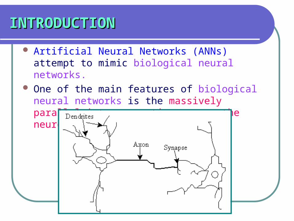
Artificial Neural Networks (ANNs) attempt to mimic biological neural networks.

One of the main features of biological neural networks is the massively parallel interconnections among the neurons.


Computational model of a biological Computational model of a biological neural network:neural network: simple operations such as:simple operations such as:

inner product computationthresholding

design parametersdesign parameters 1.1. network topology:

i.i.number of layers ii.ii.number of nodes in a layer

2.2. connection weights 3.3. property at a node; e.g.type of non-

linearity to be used.


∑

x1

x2

x3

....

xd

w1

w2

w3

wd

∑ wi . xi

Non-Linearityy

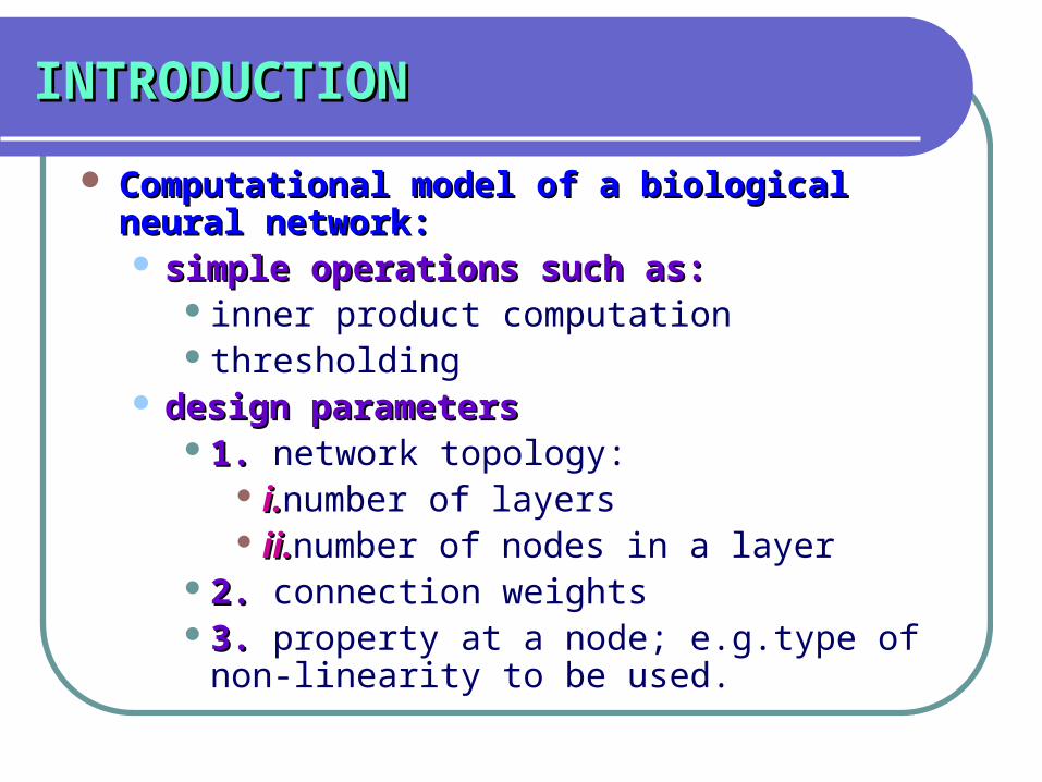
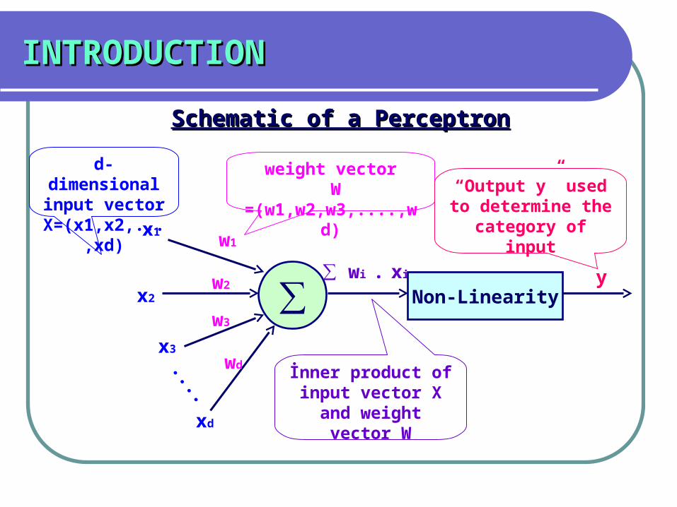
d-dimensional input vector

X=(x1,x2,...,xd)

weight vector W =(w1,w2,w3,....,wd)

İnner product of input vector X and weight vector W

“Output y” used to determine the

category of input

Schematic of a PerceptronSchematic of a Perceptron

INTRODUCTION:INTRODUCTION:

Multilayer Perceptrons: (MLPs)Multilayer Perceptrons: (MLPs) one of the most popular neural network models

for solving pattern classification and image classification problems

consists of several layer of perceptrons nodes in the i layer are connected to nodes in

the (i+1) layer through suitable weights no interconnection among the nodes in a layer.

th

th

INTRODUCTION:INTRODUCTION: Multilayer PerceptronsMultilayer Perceptrons

Multilayer Perceptron Biological neuron


Training of a MLP:Training of a MLP: 1.Feedforward Stage:1.Feedforward Stage:

training patterns with known class labels are training patterns with known class labels are presented at the input layer presented at the input layer

at the start weight matrix is randomly at the start weight matrix is randomly initialisedinitialised

the output is computed at the output node.the output is computed at the output node. 2.Weight Update Stage:2.Weight Update Stage:

weights are updated in a backward fashion weights are updated in a backward fashion starting with the output layerstarting with the output layer

weights are changed proportional to the weights are changed proportional to the error between the desired output and the error between the desired output and the actual output.actual output.

3.Repeat 1 and 2 until the network converges3.Repeat 1 and 2 until the network converges


.

.

.

x1

x2

x3

xd

Fea

ture

Vec

tor

.

.

.

.

.

.

.

.

input layer hidden layer output layer

A Multilayer Perceptron


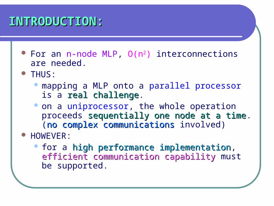
For an n-node MLP, O(n2) interconnections are needed.

THUS: mapping a MLP onto a parallel processor is a

real challengereal challenge. on a uniprocessor, the whole operation

proceeds sequentially one node at a timesequentially one node at a time. (no complex communicationsno complex communications involved)

HOWEVER: for a high performance implementationhigh performance implementation,

efficient communication capabilityefficient communication capability must be supported.


Typical Pattern Recognition and Computer Typical Pattern Recognition and Computer Vision Applications: Vision Applications: applications have applications have >100 input nodes>100 input nodes classification process involving complex classification process involving complex

decision boundaries demands decision boundaries demands a large a large number of hidden nodesnumber of hidden nodes


Real Time Computer Vision Applications:Real Time Computer Vision Applications: The The network trainingnetwork training can be carried out can be carried out offlineoffline.. Recall Phase:Recall Phase:High input/output bandwidth is High input/output bandwidth is

required along with fast classification (recall) required along with fast classification (recall) speeds.speeds.


For a three layer network (excluding the input For a three layer network (excluding the input layer),layer),let :let :

m:m:input nodesinput nodes nn11::nodes in the first hidden layernodes in the first hidden layer nn22::nodes in the second hidden layernodes in the second hidden layer k:k:output nodes (classes)output nodes (classes) NNmm: : the number of multiplicationsthe number of multiplications NNaa::the number of additionsthe number of additions

Nm=(m*n1)+(n1*n2)+(n2*k)Na=Nm-(n1+n2+k))

Nonlinearity not included


Example- a Practical Vision SystemExample- a Practical Vision System Process a 1024 x 1024 image in “real time” 30 frames to be processed per second 30 x 1024 x 1024 =30 x 1030 x 1024 x 1024 =30 x 1066 input patterns/sec THUS, a real time neural network classifier is

expected to perform billions of operations per second.

Connection weights are floating point numbers floating point multiplications and additions

Result:Throughputs of this kind are difficult to achieve with today’s most powerful uniprocessors.


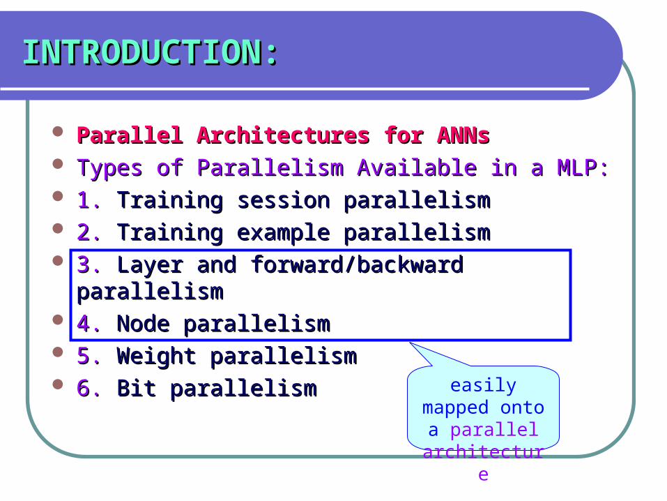
Parallel Architectures for ANNsParallel Architectures for ANNs Types of Parallelism Available in a MLP:Types of Parallelism Available in a MLP: 1. 1. Training session parallelismTraining session parallelism 2. 2. Training example parallelismTraining example parallelism 3. 3. Layer and forward/backward parallelismLayer and forward/backward parallelism 4. 4. Node parallelismNode parallelism 5. 5. Weight parallelismWeight parallelism 6. 6. Bit parallelismBit parallelism

easily mapped onto a parallel architecture


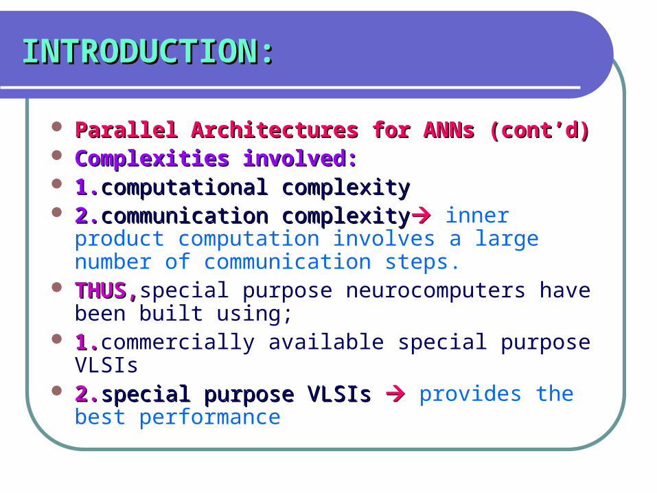
Parallel Architectures for ANNs (cont’d)Parallel Architectures for ANNs (cont’d) Complexities involved:Complexities involved: 1.1.computational complexitycomputational complexity 2.2.communication complexitycommunication complexity inner product

computation involves a large number of communication steps.

THUS,THUS,special purpose neurocomputers have been built using;

1.1.commercially available special purpose VLSIs 2.2.special purpose VLSIs special purpose VLSIs provides the best

performance


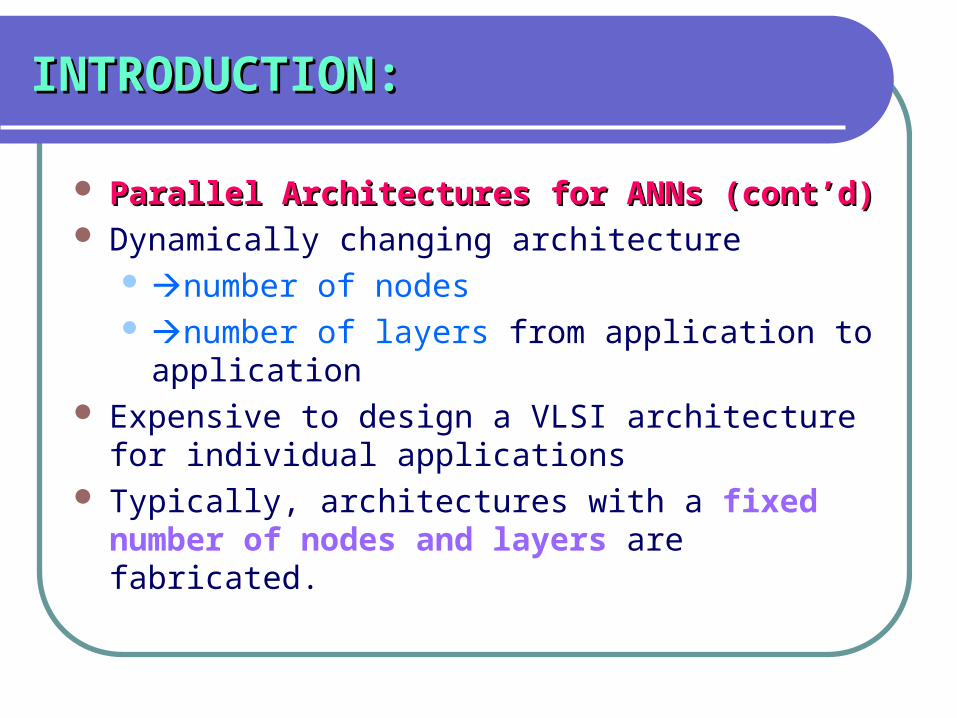
Parallel Architectures for ANNs (cont’d)Parallel Architectures for ANNs (cont’d) Dynamically changing architecture

number of nodes number of layers from application to

application Expensive to design a VLSI architecture for

individual applications Typically, architectures with a fixed number

of nodes and layers are fabricated.


Parallel Architectures for ANNs (cont’d)Parallel Architectures for ANNs (cont’d) Special Purpose ANN Implementations in the Special Purpose ANN Implementations in the

LiteratureLiterature Ghosh and Hwang:Ghosh and Hwang: investigate architectural requirements for

simulating ANNs using massively parallel massively parallel multipocessorsmultipocessors

propose a model for mapping neural networks onto message passing multicomputersmessage passing multicomputers..


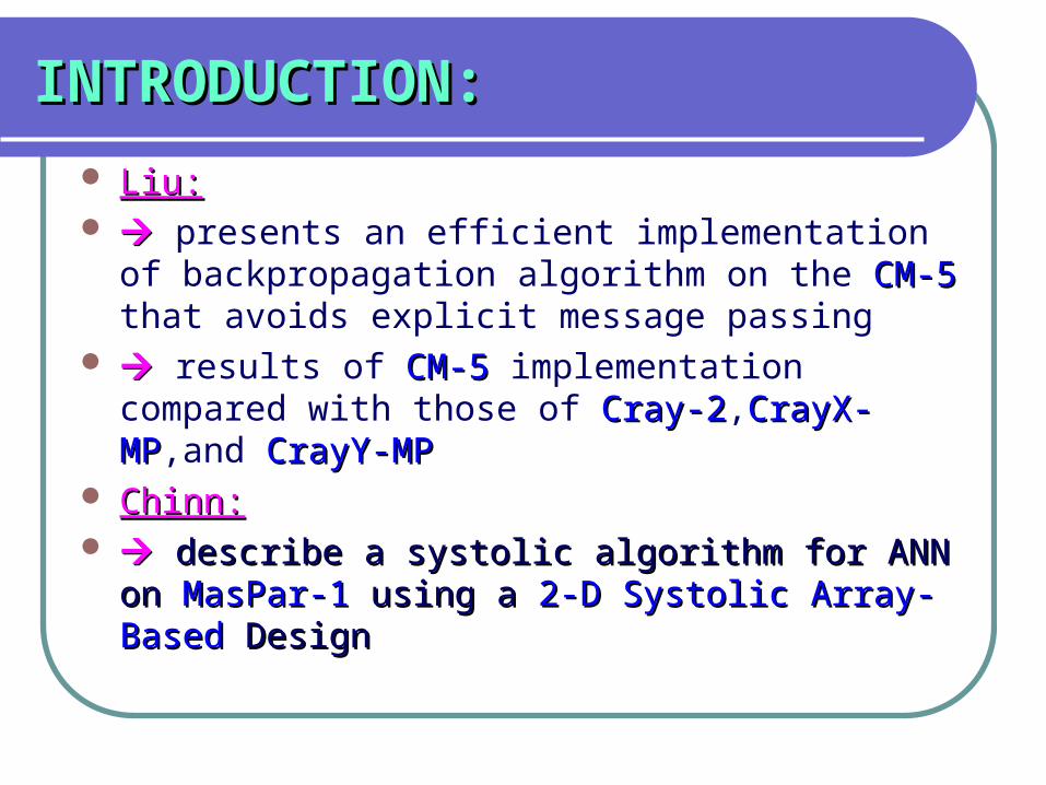
Liu:Liu: presents an efficient implementation of

backpropagation algorithm on the CM-5CM-5 that avoids explicit message passing

results of CM-5CM-5 implementation compared with those of Cray-2Cray-2,CrayX-MPCrayX-MP,and CrayY-MPCrayY-MP

Chinn:Chinn: describe a systolic algorithm for ANN on describe a systolic algorithm for ANN on

MasPar-1MasPar-1 using a using a 2-D Systolic Array-Based2-D Systolic Array-Based DesignDesign


Onuki:Onuki: present a parallel implementation using a set of present a parallel implementation using a set of

sixteen standard sixteen standard 24 bit DSPs24 bit DSPs connected in a connected in a hypercubehypercube

Kirsanov:Kirsanov: discusses a new architecture for ANNs using discusses a new architecture for ANNs using

TransputersTransputers Muller:Muller: presents a special purpose parallel computer presents a special purpose parallel computer

using a large number of using a large number of Motorola floating point Motorola floating point processorsprocessors for ANN implementation. for ANN implementation.


Parallel Architectures for ANNs (cont’d)Parallel Architectures for ANNs (cont’d) Special Purpose VLSI chips designed & fabricated Special Purpose VLSI chips designed & fabricated

for ANN implementations:for ANN implementations: Hamerstorm:Hamerstorm: a high performance and low cost ANN with:a high performance and low cost ANN with:

64 processing nodes per chip64 processing nodes per chip hardware based multiply and accumulator hardware based multiply and accumulator

operatorsoperators Barber:Barber: used used a binary tree addera binary tree adder following parallel following parallel

multipliers in multipliers in SPIN-LSPIN-L architecture architecture


Shinokawa:Shinokawa: describe a fast ANN with billion connections

per second using ASIC VLSI chips Viredez: describes MANTRA-I neurocomputer

using 2x2 systolic PE blocks Kotolainen: proposed a tree of connection units with

processing units at the leaf nodes for mapping many common ANNs.


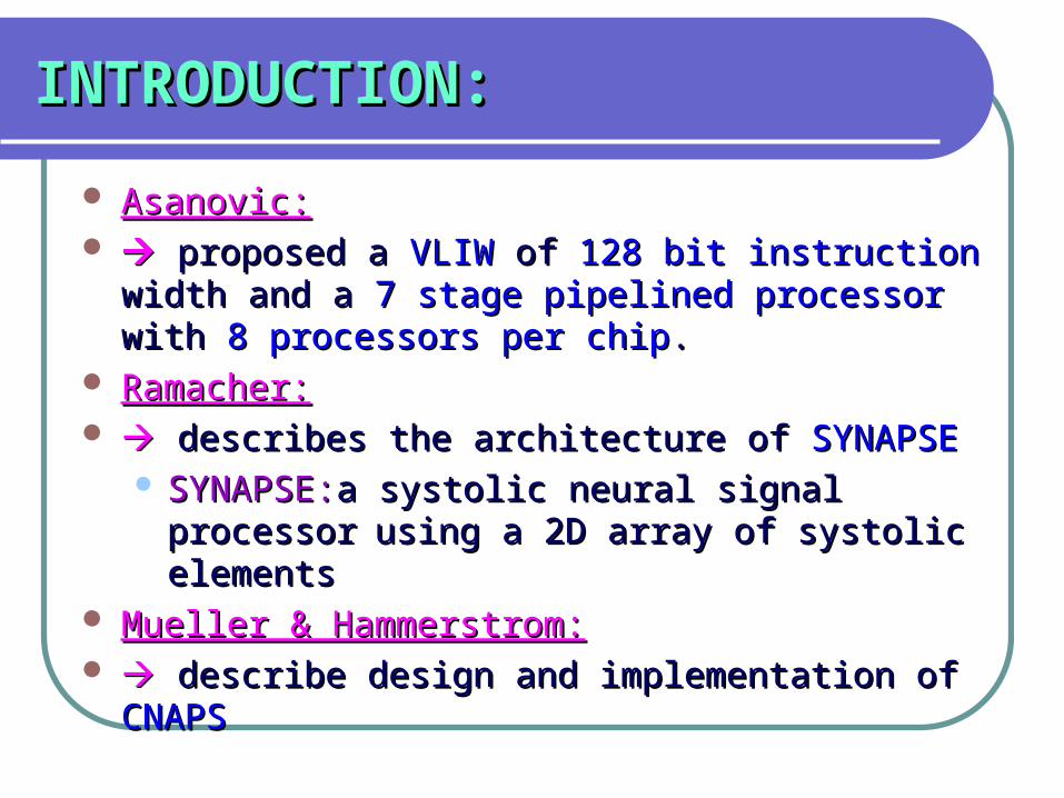
Asanovic:Asanovic: proposed a proposed a VLIWVLIW of of 128 bit instruction128 bit instruction width width

and a and a 7 stage pipelined processor7 stage pipelined processor with with 8 8 processors per chipprocessors per chip..

Ramacher:Ramacher: describes the architecture of describes the architecture of SYNAPSESYNAPSE

SYNAPSE:SYNAPSE:a systolic neural signal processora systolic neural signal processor

using a 2D array of systolic elementsusing a 2D array of systolic elements Mueller & Hammerstrom:Mueller & Hammerstrom: describe design and implementation of describe design and implementation of

CNAPSCNAPS


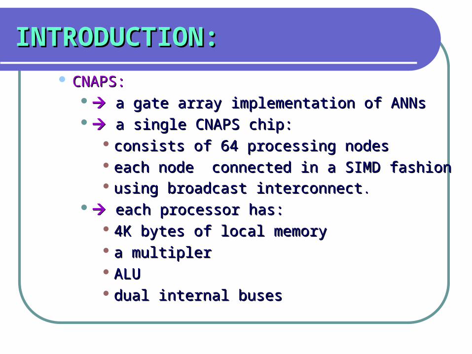
CNAPS:CNAPS: a gate array implementation of ANNsa gate array implementation of ANNs a single CNAPS chip:a single CNAPS chip:

consists of 64 processing nodesconsists of 64 processing nodes each node connected in a SIMD fashioneach node connected in a SIMD fashion using broadcast interconnectusing broadcast interconnect..

each processor has:each processor has: 4K bytes of local memory4K bytes of local memory a multiplera multipler ALUALU dual internal busesdual internal buses


Cox:Cox: describes the implementation of describes the implementation of GANGLIONGANGLION

GANGLION:GANGLION: a single neuron caters a fixed neural a single neuron caters a fixed neural

architecture of architecture of 12 input nodes12 input nodes 14 hidden nodes14 hidden nodes 4 output nodes4 output nodes

using CLBs 8x8 multipliers have been using CLBs 8x8 multipliers have been builtbuilt

a lookup table is used for the activation a lookup table is used for the activation function.function.

INTRODUCTION:INTRODUCTION: Stochastic Neural Architectures:Stochastic Neural Architectures: There is no need for a time-consuming and area

costly floating point multiplier. Suitable for VLSI implementations ExamplesExamples:: Armstrong & Thomas:Armstrong & Thomas: proposed a variation of ANN called proposed a variation of ANN called Adaptive Logic Adaptive Logic

Network (ALNs) Network (ALNs) ALNs: ALNs: similiar to ANNssimiliar to ANNs

costly multiplications replaced by costly multiplications replaced by logical logical andand operations operations

additions replaced byadditions replaced by logical logical oror operations operations


Masa Masa et. al.:et. al.: Describe an ANN,Describe an ANN,

with with a single output a single output

six hidden layerssix hidden layers

seventy inputsseventy inputs can operate at 50 MHz input ratecan operate at 50 MHz input rate

CUSTOM COMPUTING MACHINESCUSTOM COMPUTING MACHINES

Uniprocessor:Uniprocessor: instruction set available to a programmer is fixed an algorithm is coded using a sequence of

instructions processor can serve many applications by simply

reordering the sequence of instructions Application Specific Integrated Circuits (ASICs) used for a specific application provide higher performance compared to the

general purpose uniprocessor


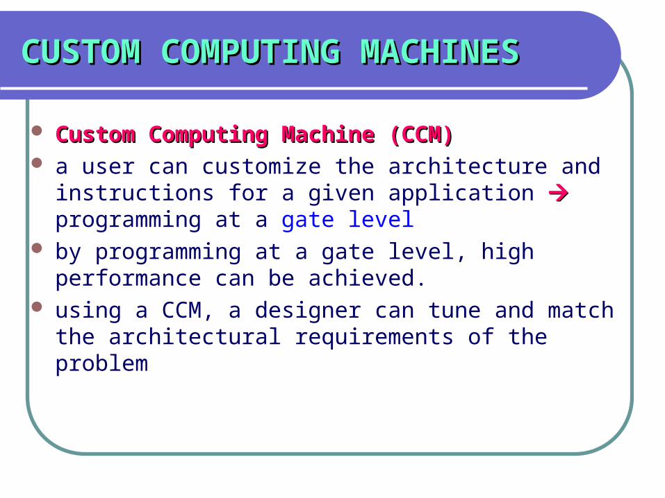
Custom Computing Machine (CCM)Custom Computing Machine (CCM) a user can customize the architecture and

instructions for a given application programming at a gate level

by programming at a gate level, high performance can be achieved.

using a CCM, a designer can tune and match the architectural requirements of the problem


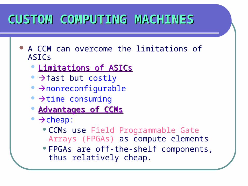
A CCM can overcome the limitations of ASICs Limitations of ASICsLimitations of ASICs fast but costly nonreconfigurable time consuming Advantages of CCMsAdvantages of CCMs cheap:

CCMs use Field Programmable Gate Arrays (FPGAs) as compute elements

FPGAs are off-the-shelf components, thus relatively cheap.


Advantages of CCMs (cont’d)Advantages of CCMs (cont’d) reconfigurable: since FPGAs are

reconfigurable, CCMs are easily reprogrammed. time saving:

CCMs do not need to be fabricated with every new application since they are often employed for fast prototyping

THUS they save a considerable amount of time in design and implementation of algorithms.

SPLASH 2 – ARCHITECTURE and SPLASH 2 – ARCHITECTURE and PROGRAMMING FLOWPROGRAMMING FLOW

Splash 2 is one of the leading FPGA based custom computing machine designed and developed by Supercomputing Research Center

SYSTEM LEVEL VIEW of the SPLASH 2 SYSTEM LEVEL VIEW of the SPLASH 2 ARCHITECTUREARCHITECTURE

interface board: 1.connects Splash 2 to the host 2.Extends the address and data buses

The Sun host can read/write to memories and memory mapped control registers of Splash 2 via these buses.

Splash 2 Processing Board

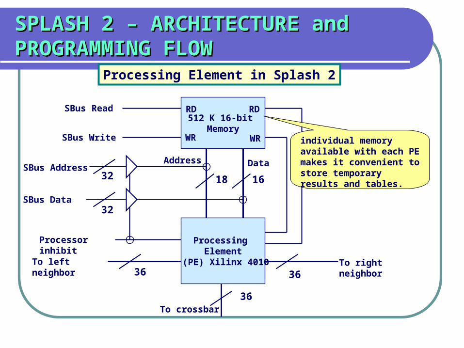
Processing Element (PE): Each PE has 512 KB of memoryThe host can read/write this memory

PEs (X1-X16)PE X0 :controls the data flow into the processor board


36

3636

32

32 18 16

512 K 16-bit Memory

RD RD

WRWR

Processing Element

(PE) Xilinx 4010

SBus Read

SBus Write

SBus Address

SBus Data

Processor inhibit

To left neighbor To right neighbor

To crossbar

Address Data

Processing Element in Splash 2

individual memory available with each PE makes it convenient to store temporary results and tables.


Logic Synthesis(Gate level decription)

Timing of logic

Simulation

Splash 2

Partition, place and route

(Logic placement)

VHDL source

Programming Flow for Splash 2

Logic designed using VHDL is verified.

Main concern:achieve the bestplacement of logicin an FPGA in order to minimize timing delay.

if the logic circuit can not be mapped to CLBs and flip flops which are available internal to anFPGA , then designer needs to revise the logic in the VHDL code and the process is repeated.

Once the logic is mapped to CLBs, thetiming for the entire

digital logic is obtained.

İf timing obtained isnot acceptable thendesign process is repeated.

To program Splash 2, weneed to program: 1. Each of the PEs2. Crossbar3. Host interface

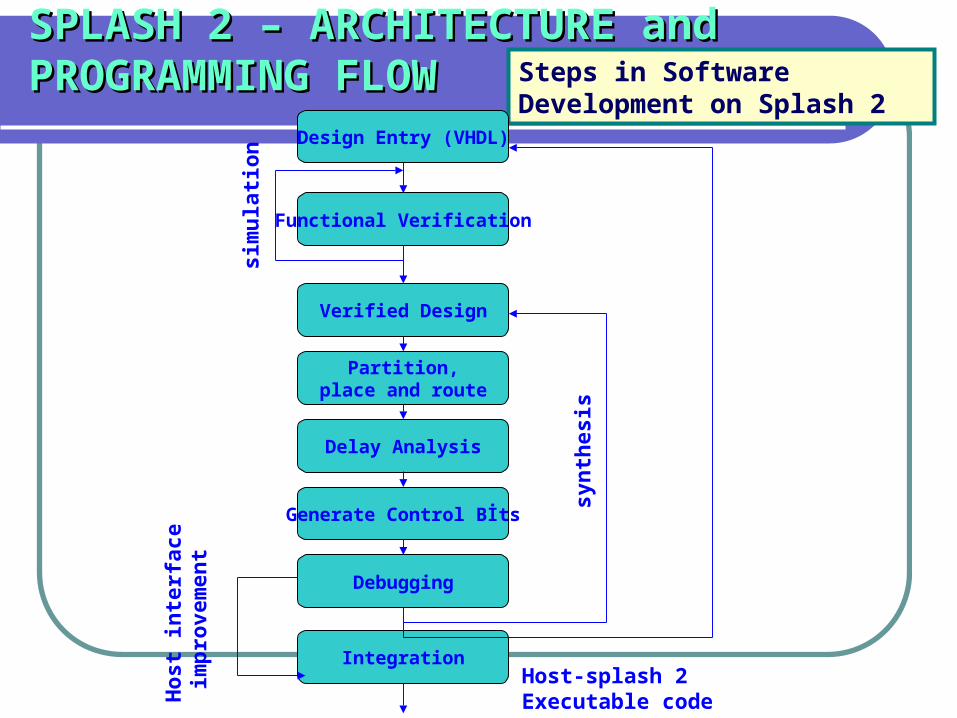
SPLASH 2 – ARCHITECTURE and SPLASH 2 – ARCHITECTURE and PROGRAMMING FLOWPROGRAMMING FLOW Steps in Software

Development on Splash 2Design Entry (VHDL)

Functional Verification

sim

ula

tio

n

Verified Design

Partition,place and route

Delay Analysis

Generate Control Bİts

Debugging

Integration

syn

thes

is

Ho

st in

terf

ace

imp

rove

men

t

Host-splash 2 Executable code

MAPPING an MLP on SPLASH 2MAPPING an MLP on SPLASH 2

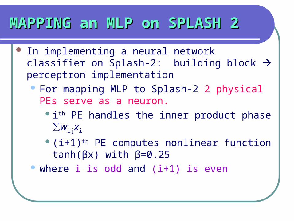
In implementing a neural network classifier on Splash-2: building block perceptron implementation For mapping MLP to Splash-2 2 physical PEs serve

as a neuron. ith PE handles the inner product phase ∑wijxi

(i+1)th PE computes nonlinear function tanh(βx) with β=0.25

where i is odd and (i+1) is even


Assume: perceptrons have been trained connection weights are fixed. Thus, an efficient way of handling the multiplication

is to employ a Look-up Table.Since a large external memory (512 KB),the lookup table can be stored.

A pattern vector component xi is presented at every clock cycle

1. Inner Product Calculation: The ith (odd) PE look up the multiplication table to

obtain the weighted product


The sum ∑wijxi is computed using an accumulator. After all the components of a pattern vector have

been examined, we have computed the inner product.

2. Application of nonlinear function to the inner product The nonlinearity is again stored as a lookup table in

the second PE. On receiving the inner product result from the first

PE, the second uses the result as the address to the non-linearity look-up table and produces the output.


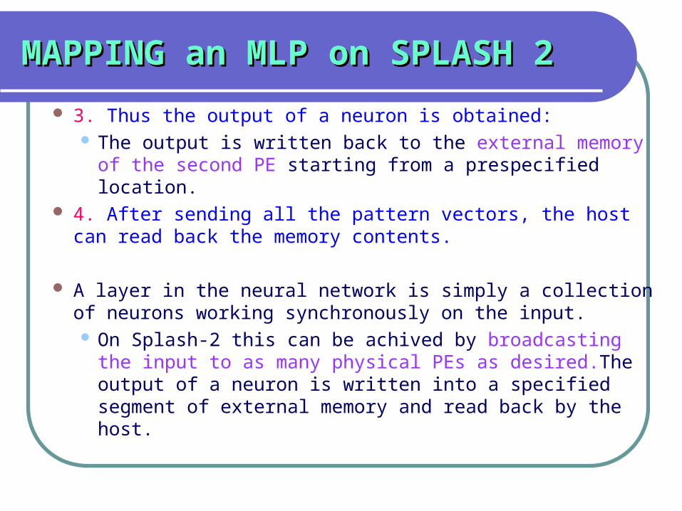
3. Thus the output of a neuron is obtained: The output is written back to the external memory of

the second PE starting from a prespecified location. 4. After sending all the pattern vectors, the host can read

back the memory contents.

A layer in the neural network is simply a collection of neurons working synchronously on the input. On Splash-2 this can be achived by broadcasting the

input to as many physical PEs as desired.The output of a neuron is written into a specified segment of external memory and read back by the host.


For every layer in MLP stages 1-4 is repated until the output layer is reached.

NOTE: For every layer, there is a different look-up table.

Look-up Table Organization: There are m multiplicationsm multiplications to be performed per

node corresponding to the m-dimensional weightm-dimensional weight vector.

Look-up Table is divided into m segments.


Look-up Table Organization (cont’d) A counter is incremented at every clock which forms the

higher order (block) address for the lookup table.

Note:The offset can also be negative correponding to a negative input to the look up table.

Table m

:

Table 1

Block Offset17 12

11 0

•Pattern vector componentforms the lower order address bits.•Splash-2 has 18 bit adress bus for the external memory.

•Higher order 6 bits for the block address •Lower order 12 bits for the offset

address within the block.


Look-up Table Organization (cont’d) The numbers have been represented by 12 bits 2’s

complement representation. Hence; The resolution of this representation is eleven bits.

accumulator: within PE 16 bit wide

After accumulation, the accumulator result is scaled down to 12 bits.

MAPPING an MLP on SPLASH 2MAPPING an MLP on SPLASH 2Lookup Table Organization

PERFORMANCE EVALUATIONPERFORMANCE EVALUATION

The requirements for mapping a MLP required to complete a classification process: in terms of PEs required number of PEs required is equal to twice the

number of layers in each layer. number of clock cycles required = m*K* l where: m: number of input layer nodes. K: number of patterns l :number of clock cycles


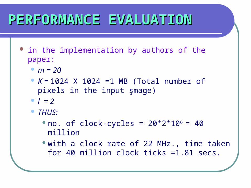
in the implementation by authors of the paper: m = 20 K = 1024 X 1024 =1 MB (Total number of pixels in

the input şmage) l = 2 THUS:

no. of clock-cycles = 20*2*106 = 40 millionwith a clock rate of 22 MHz., time taken for 40

million clock ticks =1.81 secs.


When the number of PEs required is larger than the available PEs; either more processor boards need to be added or PEs need to be time shared.

NOTE:NOTE: neuron outputs are produced independent of

other neurons algorithm waits till the computations in each

layer is completed.


A MLP has communication complexity of O(n2) where n is the number of nodes.

As n grows, it will be difficult to get good timing performance from a single processor system.

with a large number of processor boards, the single input data bus of 36 bits can cater to multiple input patterns. Note: In a multiboard system, all boards receive the same

input. This parallelism can give rise to more data

streaming into the system, thus the number of clock cycles is reduced.


splashsplash

sparc20sparc20

Size of networkSize of network

Tim

e (L

og

Sca

le)

Tim

e (L

og

Sca

le)

SCALABILITY:SCALABILITY:only a single layer isconsiderednetwork size is represented by the # of nodes in that layersmultilayered networks are considered to be linearly scalable in Splash 2 architectureperformance measure isprocessing time asmeasured by # of clock cycles for Splash 2 with 22 MHz. Clock.


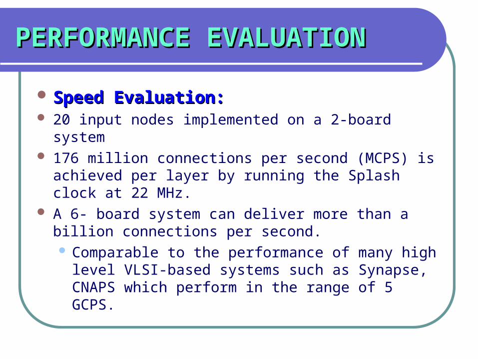
Speed Evaluation:Speed Evaluation: 20 input nodes implemented on a 2-board system 176 million connections per second (MCPS) is

achieved per layer by running the Splash clock at 22 MHz.

A 6- board system can deliver more than a billion connections per second. Comparable to the performance of many high level

VLSI-based systems such as Synapse, CNAPS which perform in the range of 5 GCPS.


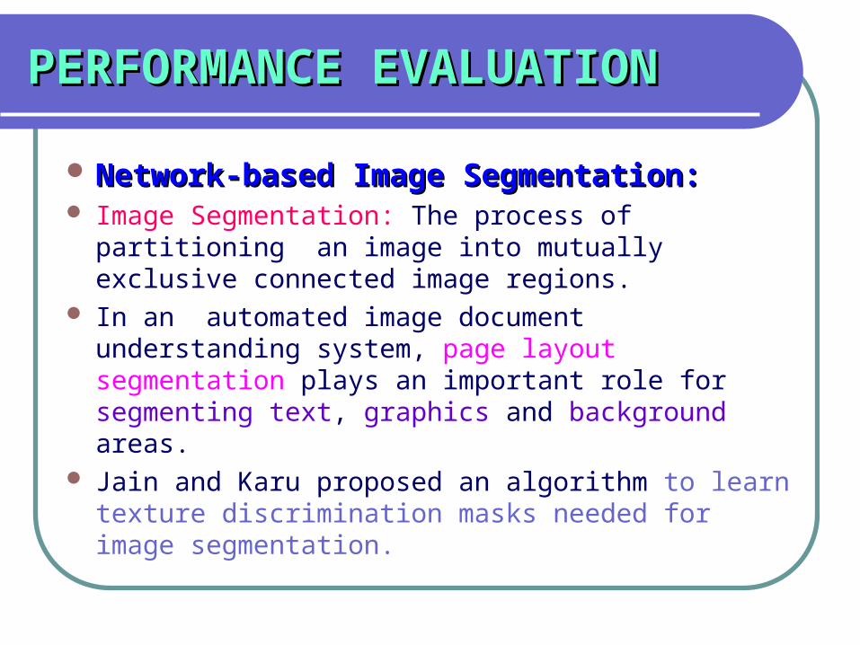
Network-based Image Segmentation:Network-based Image Segmentation: Image Segmentation: The process of partitioning an

image into mutually exclusive connected image regions.

In an automated image document understanding system, page layout segmentation plays an important role for segmenting text, graphics and background areas.

Jain and Karu proposed an algorithm to learn texture discrimination masks needed for image segmentation.


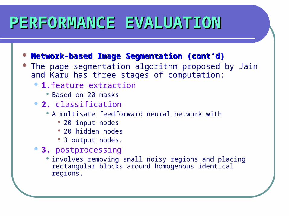
Network-based Image Segmentation (cont’d)Network-based Image Segmentation (cont’d) The page segmentation algorithm proposed by Jain and

Karu has three stages of computation: 1.feature extraction

Based on 20 masks 2. classification

A multisate feedforward neural network with 20 input nodes 20 hidden nodes 3 output nodes.

3. postprocessing involves removing small noisy regions and placing rectangular

blocks around homogenous identical regions.

PERFORMANCE EVALUATIONPERFORMANCE EVALUATION Network-based Image Segmentation (cont’d)Network-based Image Segmentation (cont’d)

Schematic of the Page Segmentation AlgorithmSchematic of the Page Segmentation Algorithm

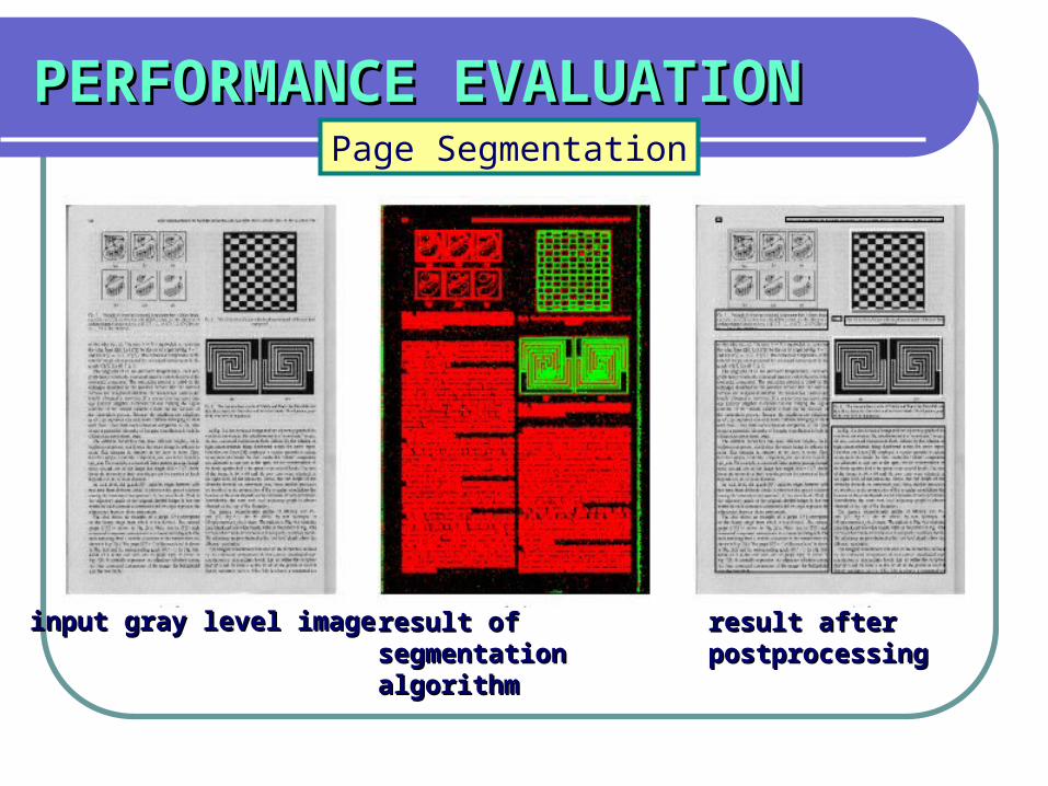
PERFORMANCE EVALUATIONPERFORMANCE EVALUATIONPage Segmentation

input gray level imageinput gray level image result of segmentation result of segmentation algorithmalgorithm

result after result after postprocessingpostprocessing

CONCLUSIONS:CONCLUSIONS:

A novel sheme of mapping MLPs on Custom Computing Machine has been presented.

The scheme is scalable in terms of number of nodes and the number of layers in the MLP and provides near-ASIC level speed.

The reconfigurality of CCMs has been exploited to map several layers of a MLP onto the same hardware.

The performance gains achieved using this mapping have been demonstrated on a network-based image segmentation.

HIGH PERFORMANCE MULTILAYER PERCEPTRON ON A CUSTOM COMPUTING MACHINE Authors: Nalini K. Ratha, Anil...

Documents

Transcript of HIGH PERFORMANCE MULTILAYER PERCEPTRON ON A CUSTOM COMPUTING MACHINE Authors: Nalini K. Ratha, Anil...