High-Performance Heterogeneous Computing || Implementation Issues
38
111 CHAPTER 7 Implementation Issues 7.1 PORTABLE IMPLEMENTATION OF HETEROGENEOUS ALGORITHMS AND SELF-ADAPTABLE APPLICATIONS Parallel programming for heterogeneous platforms is a more difficult and challenging task than that for traditional homogeneous ones. The heterogene- ity of processors means that they can execute the same code at different speeds. The heterogeneity of communication networks means that different communication links may have different bandwidths and latency. As a result, traditional parallel algorithms that distribute computations and communica- tions evenly over available processors and communication links will not, in general, be optimal for heterogeneous platforms. Heterogeneous algorithms can be designed to achieve top performance on heterogeneous networks of computers. Such algorithms would distribute computations and communica- tions unevenly, taking into account the heterogeneity of both the processors and the communication network. The design of heterogeneous parallel algorithms introduced in Part II of this book has been an active research area over the last decade. A number of highly efficient heterogeneous algorithms have been proposed and analyzed. At the same time, there is practically no available scientific software based on these algorithms. The prime cause of this obvious disproportion in the number of heterogeneous parallel algorithms that have been designed and the scien- tific software based on these algorithms is that the implementation of a heterogeneous parallel algorithm is itself a difficult and nontrivial task. The point is that the program implementing the algorithm only makes sense if it is portable and able to automatically tune itself to any executing heteroge- neous platform in order to achieve top performance. This poses additional challenges that should be addressed by scientific programmers. Let us take a closer look at these challenges. As we have seen in Part II of this book, a heterogeneous parallel algorithm is normally designed in a generic, parameterized form. Parameters of the algorithm can be divided into three groups (Lastovetsky, 2006): High-Performance Heterogeneous Computing, by Alexey L. Lastovetsky and Jack J. Dongarra Copyright © 2009 John Wiley & Sons, Inc.
Transcript of High-Performance Heterogeneous Computing || Implementation Issues

111
CHAPTER 7
Implementation Issues
7.1 PORTABLE IMPLEMENTATION OF HETEROGENEOUS ALGORITHMS AND SELF - ADAPTABLE APPLICATIONS
Parallel programming for heterogeneous platforms is a more diffi cult and challenging task than that for traditional homogeneous ones. The heterogene-ity of processors means that they can execute the same code at different speeds. The heterogeneity of communication networks means that different communication links may have different bandwidths and latency. As a result, traditional parallel algorithms that distribute computations and communica-tions evenly over available processors and communication links will not, in general, be optimal for heterogeneous platforms. Heterogeneous algorithms can be designed to achieve top performance on heterogeneous networks of computers. Such algorithms would distribute computations and communica-tions unevenly, taking into account the heterogeneity of both the processors and the communication network.
The design of heterogeneous parallel algorithms introduced in Part II of this book has been an active research area over the last decade. A number of highly effi cient heterogeneous algorithms have been proposed and analyzed. At the same time, there is practically no available scientifi c software based on these algorithms. The prime cause of this obvious disproportion in the number of heterogeneous parallel algorithms that have been designed and the scien-tifi c software based on these algorithms is that the implementation of a heterogeneous parallel algorithm is itself a diffi cult and nontrivial task. The point is that the program implementing the algorithm only makes sense if it is portable and able to automatically tune itself to any executing heteroge-neous platform in order to achieve top performance. This poses additional challenges that should be addressed by scientifi c programmers. Let us take a closer look at these challenges.
As we have seen in Part II of this book, a heterogeneous parallel algorithm is normally designed in a generic, parameterized form. Parameters of the algorithm can be divided into three groups (Lastovetsky, 2006 ):
High-Performance Heterogeneous Computing, by Alexey L. Lastovetsky and Jack J. DongarraCopyright © 2009 John Wiley & Sons, Inc.

112 IMPLEMENTATION ISSUES
• problem parameters, • algorithmic parameters, and • platform parameters.
Problem parameters are the parameters of the problem to be solved (e.g., the size of the matrix to be factorized). These parameters can only be provided by the user.
Algorithmic parameters are the parameters representing different varia-tions and confi gurations of the algorithm. Examples are the size of a matrix block in local computations for linear algebra algorithms, the total number of processes executing the algorithm, and the logical shape of their arrangement. The parameters do not change the result of computations but can have an impact on the performance. This impact may be very signifi cant. On some platforms, a multifold speedup can be achieved due to the optimization of the algorithmic parameters rather than using their default values. The infl uence of algorithmic parameters on the performance can be due to different reasons. The total amount of computations or communications can depend on some parameters such as the logical shape of how the processes are arranged. Others do not change the volume of computations and communications but can change the fraction of computations performed on data located at higher levels of memory hierarchy, and hence, change the fraction of computations performed at a higher speed (the size of a matrix block in local computations for linear algebra algorithms is of this type). The program straightforwardly implementing the algorithm would require its users to provide (optimal) values of such parameters. This is the easiest way for the scientifi c programmer to implement the algorithm, but it makes the use of the program rather incon-venient. An alternative approach, which is more convenient for the end users, is to delegate the task of fi nding the optimal values of the algorithmic param-eters to the software implementing the algorithm, making the software self - adaptable to different heterogeneous platforms.
Platform parameters are the parameters of the performance model of the executing heterogeneous platform such as the speed of the processes and the bandwidth and latency of communication links between the processes. The parameters have a major impact on the performance of the program imple-menting the algorithm. Indeed, consider an algorithm distributing computa-tions in proportion to the speed of processors and based, say, on a simple constant performance model of heterogeneous processors. The algorithm should be provided with a set of positive constants representing the relative speed of the processors. The effi ciency of the corresponding application will strongly depend on the accuracy of estimation of the relative speed. If this estimation is not accurate enough, the load of the processors will be unbal-anced, resulting in poor execution performance.
The traditional approach to this problem is to run a test code to measure the relative speed of the processors in the network and then use this estima-tion when distributing computation across the processors. Unfortunately, the

PORTABLE IMPLEMENTATION OF HETEROGENEOUS ALGORITHMS 113
problem of accurate estimation of the relative speed of processors is not as easy as it may look. Of course, if two processors only differ in clock rate, it will not be a problem to accurately estimate their relative speed. A single test code can be used to measure their relative speed, and the relative speed will be the same for any application. This simple approach may also work if the processors used in computations have very similar architectural characteristics. But if the processors are of very different architectures, the situation will change drastically. Everything in the processors may be different: sets of instructions, number of instruction execution units, numbers of registers, struc-tures of memory hierarchy, sizes of each memory level, and so on. Therefore, the processors may demonstrate different relative speeds for different applica-tions. Moreover, processors of the same architecture but of different models or confi gurations may also demonstrate different relative speeds on different applications. Even different applications of the same narrow class may be executed by two different processors at signifi cantly different relative speeds.
Another complication comes up if the network of computers allows for multi - tasking. In this case, the processors executing the parallel application may be also used for other computations and communications. Therefore, the real performance of the processors can dynamically change depending on the external computations and communications. Accurate estimation of the plat-form parameters for more advanced performance models (using, say, the func-tional model of processors) is obviously even more a diffi cult problem.
Therefore, if scientifi c software implementing the heterogeneous algorithm requires the user to provide the platform parameters, its performance will strongly depend on the accuracy of the provided parameters, making the software rather useless for the majority of potential users. Indeed, even relatively small inaccuracies in the estimation of these parameters can completely distort the performance. For example, let only one slow processor be wrongly estimated by the user as a fast one (say, because of the use of a nonrepresen-tative test code). Then, this processor will be assigned by the software a dis-proportional large amount of computation and slow down the application as the other processors will be waiting for it at points of data transfer and synchronization.
Thus, good scientifi c software implementing a heterogeneous parallel algo-rithm should provide
• accurate platform parameters of the algorithm and • optimal values of algorithmic parameters.
If implemented this way, the application will be portable and self - adaptable, automatically tuning to the executing heterogeneous platform in order to provide top performance. In terms of implementation, this means that, in addition to the core code of the program implementing the algorithm for each valid combination of the values of its parameters, the scientifi c programmer has to write a signifi cant amount of nontrivial code responsible for the solution of the above tasks.

114 IMPLEMENTATION ISSUES
Note . It should be noted that one fundamental assumption is implicitly made about all algorithms considered in this book. Namely, we assume that the volume of computations and communications performed during the execution of an algorithm is fully determined by its problem and algorithmic parameters and does not depend on the value of input data such as matrices. Algorithms that may perform different amounts of computations or communications depending on the value of the input data are out of the scope of this book.
How can a programming system help the scientifi c programmer write all the code? First of all, it does not look realistic to expect that the programming system can signifi cantly automate the writing of the core code of the program. Actually, if this was the case, it would mean that the possibility of an automatic generation of good heterogeneous parallel algorithms from some simple speci-fi cations would be realized. As we have seen, the design of heterogeneous parallel algorithms is a very diffi cult and challenging task that is wide open for research. This research area is just taking its fi rst steps, and thus requires a lot of skill and creativity from contributors. In other words, it is unrealistic to expect that parallel programming systems for heterogeneous computing can help common users having no idea about heterogeneous parallel algorithms but are willing, with minimal efforts, to obtain a good parallel program effi -ciently solving their problems in heterogeneous environments. On the other hand, given the algorithm is well described, the implementation of the core code is rather a straightforward engineering exercise.
What the programming system can do is to help qualifi ed algorithm design-ers write the code responsible for providing accurate platform parameters and for the optimization of algorithmic parameters. The code provided by the programming system comes in two forms. The fi rst one is the application - specifi c code generated by a compiler from the specifi cation of the imple-mented algorithm provided by the application programmer. The second type of code is not application specifi c and comes in the form of run - time support systems and libraries. It is worthwhile to note that the size and complexity of such code is very signifi cant and can account for more than 90% of the total code for some algorithms.
Programming systems for heterogeneous parallel computing can help not only in the implementation of original heterogeneous parallel algorithms but also in the effi cient implementation of traditional homogeneous parallel algorithms for heterogeneous platforms. This approach can be summarized as follows:
• The whole computation is partitioned into a large number of equal chunks. • Each chunk is performed by a separate process. • The number of processes run by each processor is proportional to the
relative speed of the processor.
Thus, while distributed evenly across parallel processes, data and computa-tions are distributed unevenly over processors of the heterogeneous network

PERFORMANCE MODELS OF HETEROGENEOUS PLATFORMS 115
so that each processor performs the volume of computations proportional to its speed. Again, the code responsible for the accurate estimation of platform parameters, optimization of algorithmic parameters, and optimal mapping of processes to the processors can be provided by the programming system. The main responsibility of the application programmer is to provide an accurate specifi cation of the implemented algorithm. The practical value of this approach is that it can be used to port legacy parallel software to heterogeneous platforms.
7.2 PERFORMANCE MODELS OF HETEROGENEOUS PLATFORMS: ESTIMATION OF PARAMETERS
Accurate estimation of parameters of the performance model of the hetero-geneous platform used in the design of a heterogeneous algorithm (platform parameters) is a key to the effi cient implementation of the algorithm. If these parameters are estimated inaccurately, the heterogeneous algorithm will dis-tribute computations and communications based on wrong assumptions about the performance characteristics of the executing platform, which will result in poor performance. It can be even much poorer than the performance of the homogeneous counterpart of the algorithm. Therefore, the problem of accu-rate estimation of parameters of heterogeneous performance models is very important.
7.2.1 Estimation of Constant Performance Models of Heterogeneous Processors
As can be seen from Part II , most of the heterogeneous algorithms that have been designed so far are based on the simplest performance model, whose parameters include
• p , the number of the processors, and • S = { s 1 , s 2 , … , s p }, the relative speeds of the processors in the form of
positive constants s i , Σ ip
is= =1 1.
Although some of these algorithms are originally formulated in terms of absolute speeds of the processors, we have shown that it is not necessary and the algorithms will work correctly if reformulated in terms of relative speeds (see Note on Algorithm 3.1 in Chapter 3 ). The absolute speeds in such algo-rithms are used only to make them more intuitive.
The general approach to the estimation of relative speeds of a set of hetero-geneous processors is to run some benchmark code and use its execution time on each of the processors for calculation of their relative speeds. As we have discussed in Section 2.1 , the same heterogeneous processors can execute different applications at signifi cantly different relative speeds. Therefore, it is

116 IMPLEMENTATION ISSUES
impossible to design a single, universally applicable benchmark code. The bench-mark code accurately estimating the relative speeds of the processors is applica-tion specifi c and should be carefully designed for each particular application.
The effi ciency of the benchmark code will not be a big issue if the applica-tion is supposed to be executed multiple times on the same set of heterogeneous processors having the stable and reproducible performance characteristics. In this case, the benchmark code can be separated from the main application code and run just once in order that the obtained estimation of relative speeds could be used in all subsequent runs of the application. The execution time of the benchmark code is not that substantial in this scenario as it will be negligible compared to the total execution time of all the subsequent exe-cutions of the application.
If every execution of the application is seen unique, running in a heteroge-neous environment with different performance characteristics, the benchmark code will have to be a part of the application, being executed at run time. In this case, the effi ciency of the benchmark code becomes an issue. The overhead of the accurate estimation of the performance parameters should not exceed gains due to the use of the heterogeneous algorithm. Therefore, the amount of computations performed by the benchmark code should be relatively small compared with the main body of the application ’ s computations. At the same time, in order to accurately estimate the speeds of the processors, the bench-mark code should be representative of the main body of the code, reproducing the data layout and computations of the application during its execution.
The design of the benchmark code is relatively straightforward for data parallel applications using the one - process - per - processor confi guration and performing iterative computations such that
• The data layout is static, not changing during the execution of the algorithm
• At each iteration, the processor solves the same task of the same size performing the same computations; the processed data may be different for different iterations but will still have the same pattern
• For all processors, the size of the task solved by one iteration of the main loop will be the same
In this case, the benchmark code made of any one iteration of the main loop of the implemented algorithm will be both effi cient and well representa-tive of the application. Let us illustrate this design with an application that we used in Section 3.1 . This application implements a heterogeneous parallel algorithm of multiplication of two dense square n × n matrices, C = A × B , on p processors based on one - dimensional partitioning of matrices A and C into p horizontal slices (see Fig. 3.1 ). There is one - to - one mapping between these slices and the processors. All the processors compute their C slices in parallel by executing a loop, each iteration of which computes one row of the resulting matrix C by multiplying the row of matrix A by matrix B .

PERFORMANCE MODELS OF HETEROGENEOUS PLATFORMS 117
In this application, the size of the task solved by one iteration of the main loop will be the same for all processors because the task is the multiplication of an n - element row by an n × n matrix. The load of the heterogeneous pro-cessors will be balanced by different numbers of iterations of the main loop performed by different processors. The execution time of computations per-formed by a processor will be equal to the execution time of multiplication of an n - element row by an n × n matrix multiplied by the number of iterations. Therefore, the relative speed demonstrated by the processors during the exe-cution of this application will be equal to their relative speed of the multiplica-tion of an n - element row by an n × n matrix.
Although the execution of the above benchmark code typically takes just a small fraction of the execution of the whole application, it can be made even more effi cient. Indeed, the relative speed of the processors demonstrated during the multiplication of an n - element row by an n × n matrix should be equal to their relative speed of multiplication of an n - element row by an n - element column of the matrix. Therefore, the relative speed of the processors for this application can be measured by multiplying an n - element row by an n - element column, given the column used in this computation is one of the columns of a whole n × n matrix stored in the memory of the processor. The latter requirement is necessary in order to reproduce in the benchmark code the same pattern of access to the memory hierarchy as in the original applica-tion. In practice, this more effi cient benchmark code can be too lightweight and less accurate due to possible minor fl uctuations in the load of the proces-sors. The optimal solution would be the multiplication of a row by a number of columns of the matrix. The number should be the smallest number that guarantees the required accuracy of the estimation.
Relaxation of the above restrictions on applications makes the design of the benchmark code less straightforward. Indeed, let us remove the third bulleted restriction allowing at one iteration different processors to solve tasks of different sizes. This relaxation will lead to the additional problem of fi nding the most representative task size of the benchmark. To illustrate this problem, consider the application that implements a heterogeneous parallel algorithm of multiplication of two dense square n × n matrices, C = A × B , on p proces-sors based on the Cartesian partitioning of the matrices, which was presented in Section 3.4 (see Fig. 3.13 ). The algorithm can be summarized as follows:
• Matrices A , B , and C are identically partitioned into a Cartesian partition-ing such that � There is one - to - one mapping between the rectangles of the partitioning
and the processors � The shape of the partitioning, p = q × t , minimizes ( q + t ) � The sizes of the rectangles, h i and w j , are returned by Algorithm 3.5
• At each step k of the algorithm � The pivot column of r × r blocks of matrix A , a • k , is broadcast horizontally

118 IMPLEMENTATION ISSUES
� The pivot row of r × r blocks of matrix B , b k • , is broadcast vertically � Each processor P ij updates its rectangle c ij of matrix C with the product
of its parts of the pivot column and the pivot row, c ij = c ij + a ik × b kj
In that application, at each iteration of the main loop, processor P ij solves the same task of the same size, namely, it updates an h i × w j matrix by the product of h i × r and r × w j matrices. The arrays storing these matrices are the same at all iterations. The execution time of computations performed by the processor will be equal to the execution of the task of updating an h i × w j matrix by the product of h i × r and r × w j matrices multiplied by the total number of iterations. Therefore, the speed of the processor will be the same for the whole application and for an update of an h i × w j matrix.
Unlike the fi rst application, in this case, all processors perform the same number of iterations, and the load of the processors is balanced by using dif-ferent task sizes. Therefore, whatever task size we pick for the benchmark code updating a matrix, it will not be fully representative of the application as it does not reproduce in full the data layout and computations during the real execution. Nevertheless, for any heterogeneous platform, there will be a range of task sizes where the relative speeds of the processors do not depend signifi -cantly on the task size and can be quite accurately approximated by constants. Hence, if all matrix partitions fall into this range, then the benchmark code updating a matrix of any size from this range will accurately estimate their
relative speeds for the application. In particular, a matrix of the size
nq
nt
×
can be used in the benchmark code. Finding the optimal task size for the benchmark will be more diffi cult if at
different iterations, the processor solves tasks of different sizes. Applications implementing heterogeneous parallel LU factorization algorithms from Section 3.3 are of that type. Indeed, at each iteration of the algorithm, the main body of computations performed by the processor falls into the update �A A L U L U22 22 21 12 22 22← − = of its columns of the trailing submatrix A 22 of matrix A . The size of this submatrix and the number of columns processed by the processor will become smaller and smaller with each next step of the algorithm, asymptotically decreasing to zero. Therefore, during the execution of the application, the sizes of the task solved by each processor will vary in a very wide range — from large at initial iterations to very small at fi nal ones. It is unrealistic to assume that the relative speed of the heterogeneous proces-sors will remain constant within such a wide range of task sizes. More likely, their relative speed will gradually change as the execution proceeds. In this case, no task size will accurately estimate the relative speed of the processors for all iterations. At the same time, given that different iterations have differ-ent computation cost, we can only focus on the iterations making the major contribution to the total computation time, namely, on some number of fi rst iterations. If the sizes of the tasks solved by the processors at these iterations fall into the range where the relative speeds of the processors can be

PERFORMANCE MODELS OF HETEROGENEOUS PLATFORMS 119
approximated by constants, then the benchmark code updating a matrix of any size from this range will accurately estimate their relative speeds for the entire application.
Thus, the benchmark code solving the task of some fi xed size, which repre-sents one iteration of the main loop of the application, can be effi cient and accurate for many data parallel applications performing iterative computa-tions. This approach has been used in some parallel applications designed to automatically tune to the executing heterogeneous platform (Lastovetsky, 2002 ).
There are also programming systems providing basic support for this and other approaches to accurate estimation of relative speeds of the processors. These systems are mpC (Lastovetsky, 2002 , 2003 ), the fi rst language for het-erogeneous parallel programming, and HeteroMPI (Lastovetsky and Reddy, 2006 ), an extension of MPI for high - performance heterogeneous computing. HeteroMPI and mpC allow the application programmer to explicitly specify benchmark codes representative of computations in different parts of the application. It is assumed that the relative speed demonstrated by the proces-sors during the execution of the benchmark code will be approximately the same as the relative speed of the processors demonstrated during the execu-tion of the corresponding part of the application. It is also assumed that the time of execution of this code is much less than the time of the execution of the corresponding part of the application. The mpC application programmer uses a recon statement to specify the benchmark code and when this code should be run. During the execution of this statement, all processors execute the provided benchmark code in parallel, and the execution time elapsed on each processor is used to obtain their relative speed. Thus, the accuracy of estimation of the relative speed of the processors is fully controlled by the application programmer. Indeed, creative design of the benchmark code together with well - thought - out selection of the points and frequency of the recon statements in the program are the means for the effi cient and accurate estimation of the relative speed of the processors during each particular execu-tion of the application. In HeteroMPI, the HMPI_Recon function plays the same role as the recon statement in mpC.
7.2.2 Estimation of Functional and Band Performance Models of Heterogeneous Processors
In Chapter 4 , we discussed the limitations of constant performance models of heterogeneous processors. The main limitation is the assumption that the application fi ts into the main memory of the executing parallel processors. This assumption is quite restrictive in terms of the size of problems that can be solved by algorithms based on the constant models. Therefore, functional and band performance models were introduced. The models are more general and put no restrictions on problem size. Of course, the design of heterogeneous algorithms with these models is a more diffi cult task than that with constant

120 IMPLEMENTATION ISSUES
models, but the task is solvable. In Chapter 4 , we have presented a number of effi cient heterogeneous algorithms based on the nonconstant, mainly func-tional models.
The accurate estimation of a functional performance model can be very expensive. Indeed, in order to build the speed function of the processor for a given application with a given accuracy, the application may need to be executed for quite a large number of different task sizes. One straightforward approach is as follows:
• For simplicity, we assume that the task size is represented by a single variable, x .
• The original interval [ a , b ] of possible values of the task size variable is divided into a number of equal subintervals [ x i , x i+ 1 ]. The application is executed for each task size x i , and a piecewise linear approximation is used as the fi rst approximation of the speed function f ( x ).
• At each next step, � each current subinterval is bisected and the application is executed for
all task sizes representing the midpoints, � the speeds for these points, together with all previously obtained speeds,
are used to build the next piecewise linear approximation of f ( x ), and � this new approximation and the previous one are compared against
some error criterion. If the criterion is satisfi ed, the estimation is fi n-ished; otherwise, this step is repeated.
It is very likely to have to execute the application for quite a large number of different task sizes before the above algorithm converges. The number will increase by orders of magnitude if the task size is represented by several vari-ables. As a result, in real - life situations, this straightforward algorithm can be very expensive.
Minimizing the cost of accurate estimation of the speed function is a challenging research problem of signifi cant practical importance. The problem is wide open. The only approach proposed and studied so far (Lastovetsky, Reddy, and Higgins, 2006 ) is based on the property of heterogeneous proces-sors integrated into the network to experience constant and stochastic fl uctua-tions in the workload. As have been discussed in Chapters 1 , 2 , and 4 , this changing transient load will cause a fl uctuation in the speed of the processor in the sense that the execution time of the same task of the same size will vary for different runs at different times. The natural way to represent the inherent fl uctuations in the speed is to use a speed band rather than a speed function. The width of the band characterizes the level of fl uctuation in the performance due to changes in load over time.
The idea of the approach (Lastovetsky, Reddy, and Higgins, 2006 ) is to use this inherent inaccuracy of any approximation of the speed function in order to reduce the cost of its estimation. Indeed, any function fi tting into the speed

PERFORMANCE MODELS OF HETEROGENEOUS PLATFORMS 121
band can be considered a satisfactory approximation of the speed function. Therefore, the approach is to fi nd, experimentally, a piecewise linear approxi-mation of the speed band as shown in Figure 7.1 such that it will represent the speed function with the accuracy determined by the inherent deviation of the performance of the processor. This approximation is built using a set of few experimentally obtained points as shown in Figure 7.2 . The problem is to spend minimum experimental time to build the approximation.
The piecewise linear approximation of the speed band of the processor is built using a set of experimentally obtained points for different problem sizes. For simplicity, we assume that the problem size is represented by a single vari-able. To obtain an experimental point for a problem size x , the application is
Size of the problem
Absolu
te s
peed
Real life
Piecewise
Figure 7.1. Real - life speed band of a processor and a piecewise linear function approxi-mation of the speed band.
Size of the problem
(a) (b)
Absolu
te s
peed
Absolu
te s
peed
a b
Real lifePiecewise
Size of the problem a b
Real lifePiecewise
Figure 7.2. Piecewise linear approximation of speed bands for two processors. Circular points are experimentally obtained; square points are calculated using heuristics. (a) The speed band is built from fi ve experimental points; the application uses the memory hierarchy ineffi ciently. (b) The speed band is built from eight experimental points; the application uses memory hierarchy effi ciently.

122 IMPLEMENTATION ISSUES
executed for this problem size and the ideal execution time t ideal is measured. t ideal is defi ned as the time it would require to solve the problem on a com-pletely idle processor. For example, on Unix platforms, this information can be obtained by using the time utility or the getrusage() system call, summing the reported user and system CPU seconds a process has consumed.
The ideal speed of execution, s ideal , is then equal to the volume of computa-tions divided by t ideal . Further calculations assume given two load functions , l max ( t ) and l min ( t ), which are the maximum and minimum load averages, respec-tively, observed over increasing time periods. The load average is defi ned as the number of active processes running on the processor at any time. Given the load functions, a prediction of the maximum and minimum average load, l max,predicted ( x ) and l min,predicted ( x ), respectively, that would occur during the exe-cution of the application for the problem size x are made (note that unlike the load functions, which are functions of time, the minimum and maximum average load are functions of problem size). The creation of the functions l max ( t ) and l min ( t ) and prediction of the load averages will be explained in detail later. Using s ideal and the load averages predicted, s max ( x ) and s min ( x ), for a problem size x are calculated as follows:
s x s x l x s xs x s
max min,
min
( ) = ( ) − ( ) × ( )( ) =
ideal predicted ideal
ideall predicted idealx l x s x( ) − ( ) × ( )max, . (7.1)
The experimental point is then given by a vertical line connecting the points ( x , s max ( x )) and ( x , s min ( x )). This vertical line is called a “ cut ” of the real band. This is illustrated in Figure 7.3 (a).
The difference between the speeds s max ( x ) and s min ( x ) represents the level of fl uctuation in the speed due to changes in load during the execution of the problem size x . The piecewise linear approximation is obtained by connecting these experimental points as shown in Figure 7.3 (b). So the problem of build-ing the piecewise linear function approximation is to fi nd a set of such experi-mental points that can represent the speed band with suffi cient accuracy and at the same time spend minimum experimental time to build the piecewise linear approximation.
Mathematically, the problem of building a piecewise linear approximation is formulated as follows:
• Given the functions l min ( t ) and l max ( t ) ( l min ( t ) and l max ( t ) are functions of time characterizing the level of fl uctuation in load over time)
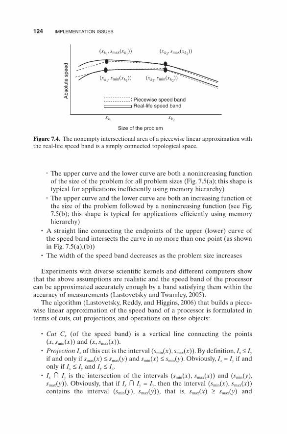
• Obtain a set of n experimental points representing a piecewise linear approximation of the speed band of a processor, each point representing a cut given by ( x i , s max ( x i )) and ( x i , s min ( x i )), where x i is the size of the problem and s max ( x i ) and s min ( x i ) are speeds calculated based on the func-tions l min ( t ) and l max ( t ) and ideal speed s ideal at point i , such that � The nonempty intersectional area of the piecewise linear approximation
with the real - life speed band is a simply connected topological space

PERFORMANCE MODELS OF HETEROGENEOUS PLATFORMS 123
(a topological space is said to be path connected if a path can be drawn from every point contained within its boundaries to every other point; a topological space is simply connected if it is path connected and has no “ holes ” ; this is illustrated in Fig. 7.4 )
� The sum tii
n
=∑
1
of the times is minimal, where t i is the experimental time
used to obtain point i
The algorithm (Lastovetsky, Reddy, and Higgins, 2006 ) returning an approxi-mate solution of this problem makes the following assumptions about the speed band:
• The upper and lower curves of the speed band are continuous functions of the problem size
• The permissible shapes of the speed band are
Size of the problem
(a)
(b)
Size of the problem
Absolu
te s
peed
Absolu
te s
peed
x
(x, smax(x))
(x1, smax(x1))
(x1, smin(x1))(x2, smin(x2))
(x3, smax(x3))
(x3, smin(x3))
(x2, smax(x2))
x1 x2 x3
(x, smin(x))
Figure 7.3. (a) The speeds s max ( x ) and s min ( x ) representing a cut of the real band used to build the piecewise linear approximation. (b) Piecewise linear approximation built by connecting the cuts .
124 IMPLEMENTATION ISSUES
� The upper curve and the lower curve are both a nonincreasing function of the size of the problem for all problem sizes (Fig. 7.5 (a); this shape is typical for applications ineffi ciently using memory hierarchy)
� The upper curve and the lower curve are both an increasing function of the size of the problem followed by a nonincreasing function (see Fig. 7.5 (b); this shape is typical for applications effi ciently using memory hierarchy)
• A straight line connecting the endpoints of the upper (lower) curve of the speed band intersects the curve in no more than one point (as shown in Fig. 7.5 (a),(b))
• The width of the speed band decreases as the problem size increases
Experiments with diverse scientifi c kernels and different computers show that the above assumptions are realistic and the speed band of the processor can be approximated accurately enough by a band satisfying them within the accuracy of measurements (Lastovetsky and Twamley, 2005 ).
The algorithm (Lastovetsky, Reddy, and Higgins, 2006 ) that builds a piece-wise linear approximation of the speed band of a processor is formulated in terms of cuts, cut projections, and operations on these objects:
• Cut C x (of the speed band) is a vertical line connecting the points ( x , s min ( x )) and ( x , s max ( x )).
• Projection I x of this cut is the interval ( s min ( x ), s max ( x )). By defi nition, I x ≤ I y if and only if s max ( x ) ≤ s max ( y ) and s min ( x ) ≤ s min ( y ). Obviously, I x = I y if and only if I x ≤ I y and I y ≤ I x .
• I x � I y is the intersection of the intervals ( s min ( x ), s max ( x )) and ( s min ( y ), s max ( y )). Obviously, that if I x � I y = I y , then the interval ( s min ( x ), s max ( x )) contains the interval ( s min ( y ), s max ( y )), that is, s max ( x ) ≥ s max ( y ) and
Size of the problem
Piecewise speed bandReal-life speed band
(xk1, smax(xk1
))
(xk1, smin(xk1
))
xk1xk2
(xk2, smin(xk2
))
(xk2, smax(xk2
))
Absolu
te s
peed
Figure 7.4. The nonempty intersectional area of a piecewise linear approximation with the real - life speed band is a simply connected topological space.

PERFORMANCE MODELS OF HETEROGENEOUS PLATFORMS 125
s min ( x ) ≤ s min ( y ). If the intervals are disjoint, then I x � I y = Ø , where Ø is an empty interval.
Algorithm 7.1 (Lastovetsky, Reddy, and Higgins, 2006 ). Building piecewise linear approximation of the speed band of a processor characterized by given load functions l max ( t ) and l min ( t ):
Step 1: Initialization. We select an interval [ a , b ] of problem sizes, where a is some small size and b is the problem size large enough to make the speed of the processor practically zero. We obtain, experimentally, the speeds of the processor at point a given by s max ( a ) and s min ( a ) and we set the speed of the processor at point b to 0. Our initial approximation of the speed band is a band connecting cuts C a and C b . This is illustrated in Figure 7.6 (a).
Size of the problem
(a)
(b)
Abso
lute
speed
Absolu
te s
peed
Real-life speed band (upper curve)Real-life speed band (lower curve)Straight line to lower curveStraight line to upper curve
Size of the problem
Real-life speed band (upper curve)Real-life speed band (lower curve)Straight line to upper curveStraight line to lower curve
Figure 7.5. Shapes of the speed bands of processors for applications ineffi ciently (a) and effi ciently (b) using memory hierarchy.

a ab
2a
3a
b
Siz
e o
f th
e p
roble
m
Siz
e o
f th
e p
roble
mS
ize o
f th
e p
roble
m
Real-lif
e s
peed function
Pie
cew
ise lin
ear
function
appro
xim
ation
Real-lif
e s
peed function
Pie
cew
ise lin
ear
function
appro
xim
ation
Siz
e o
f th
e p
roble
m
(a)
(d)
(g)
(b)
(e)
(c)
(f)
Siz
e o
f th
e p
roble
m
Siz
e o
f th
e p
roble
m
(a, s
max
(a))
((k
+ 1
) ×
a, s
max
((k
+ 1
) ×
a))
(xle
ft, s
max
(xle
ft))
(xle
ft, s
max
(xle
ft))
(xri
ght,
s max
(xri
ght)
)
(xri
ght,
0)(x
b 1, s
min
(xb 1
))
(xb 1
, sm
ax(x
b 1))
(xb 1
, sm
ax(x
b 1))
(xb 1
, sm
in(x
b 1))
(xle
ft, s
min
(xle
ft))
(xri
ght,
s max
(xri
ght)
)
(xri
ght,
0))
x rig
htx l
eft
(xle
ft, s
min
(xle
ft))
(xb 1
, sm
ax(x
b 1))
(xb 1
, sm
in(x
b 1))
(a, s
min
(a))
(b, s
max
(b)
)
(a, s
max
(a))
((k
+ 1
) ×
a, s
min
((k
+ 1
) ×
a))
(b, s
max
(b))
(b,
0)
(b,
0)
(a, s
min
(a))
Absolute speed Absolute speed Absolute speed
Absolute speedAbsolute speedAbsolute speed
Absolute speed
(k +
1)×
a x b1
x rig
htx l
eft
x b1
Siz
e o
f th
e p
roble
m
x rig
htx l
eft
x b1
x rig
htx l
eft
x b1
x rig
htx l
eft
x b1
Fig
ure
7.6.
(a)
Ini
tial
app
roxi
mat
ion
of t
he s
peed
ban
d. (
b) A
ppro
xim
atio
n of
the
incr
easi
ng s
ecti
on o
f th
e sp
eed
band
. (c
) – (e
) A
ppro
xim
atio
n of
the
non
incr
easi
ng s
ecti
on o
f th
e sp
eed
band
. (f
) an
d (g
) Po
ssib
le s
cena
rios
whe
n th
e ne
xt
expe
rim
enta
l poi
nt f
alls
in t
he a
rea
of t
he c
urre
nt t
rape
zoid
al a
ppro
xim
atio
n: (
f) t
he c
urre
nt a
ppro
xim
atio
n is
acc
urat
e;
(g)
the
curr
ent
appr
oxim
atio
n is
inac
cura
te.
126

PERFORMANCE MODELS OF HETEROGENEOUS PLATFORMS 127
Step 2: Approximation of the Increasing Part of the Speed Band (If Any). First, we experimentally fi nd cuts for problem sizes a and 2 a . If I 2 a ≤ I a or I 2 a � I a = I 2 a (i.e., the increasing section of the speed band, if any, ends at point a ), the current trapezoidal approximation is replaced by two trapezoidal connected bands, the fi rst one connecting cuts C a and C 2 a and the second one connecting cuts C 2 a and C b . Then, we set x left to 2 a and x right to b and go to Step 3 dealing with the approximation of the nonincreasing section of the band.
If I a < I 2 a (i.e., the band speed is increasing), Step 2 is recursively applied to pairs ( ka , ( k + 1) a ) until I ( k +1) a ≤ I ka or I ( k +1) a � I ka = I ( k +1) a . Then, the current trapezoidal approximation of the speed band in the interval [ ka , b ] is replaced by two connected bands, the fi rst one connecting cuts C ka and C ( k +1) × a and the second one connecting cuts C ( k +1) × a and C b . Then, we set x left to ( k + 1) a and x right to b and go to Step 3. This is illustrated in Figure 7.6 (b).
It should be noted that the experimental time taken to obtain the cuts at problem sizes { a , 2 a , 3 a , … ,( k + 1) × a } is relatively small (usually milliseconds to seconds) compared with that for larger problem sizes (usually minutes to hours).
Step 3: Approximation of the Nonincreasing Section of the Speed Band. We bisect the interval [ x left , x right ] into subintervals x xbleft, 1[ ] and x xb1, right[ ] of equal length. We obtain, experimentally, the cut Cxb1 at problem size xb1. We also calculate the cut of intersection of the line x xb= 1 with the current approximation of the speed band connecting the cuts Cx left and Cx right . The cut of the intersection is given by ′C xb1.
• If Ix Ixbleft ∩ 1 ≠ ∅ , we replace the current trapezoidal approximation of the speed band with two connected bands, the fi rst one connecting cuts Cx left and Cxb1 and the second one connecting cuts Cxb1 and Cx right . This is illustrated in Figure 7.6 (c). We stop building the approximation of the speed band in the interval x xbleft, 1[ ] and recursively apply Step 3 to the interval x xb1, right[ ].
• If Ix Ixbleft ∩ 1 = ∅ and Ix Ixbright ∩ 1 ≠ ∅ , we replace the current trapezoidal approximation of the speed band with two connected bands, the fi rst one connecting cuts Cx left and Cxb1 and the second one connecting cuts Cxb1 and Cx right . This is illustrated in Figure 7.6 (d). We stop building the approx-imation of the speed band in the interval x xb1, right[ ] and recursively apply Step 3 for the interval x xbleft, 1[ ].
• If Ix Ixbleft ∩ 1 = ∅ and Ix Ixbright ∩ 1 = ∅ and ′ <I x Ixb b1 1 (i.e., ′ ≤I x Ixb b1 1 and Ix I xb b1 1∩ ′ = ∅ ), we replace the current trapezoidal approximation of the speed band with two connected bands, the fi rst one connecting cuts Cx left and Cxb1 and the second one connecting cuts Cxb1 and Cx right . This is illustrated in Figure 7.6 (e). Then, we recursively apply Step 3 to the inter-vals x xbleft, 1[ ] and x xb1, right[ ] .

128 IMPLEMENTATION ISSUES
• If Ix Ixbleft ∩ 1 = ∅ and Ix Ixbright ∩ 1 = ∅ and Ix I xb b1 1∩ ′ ≠ ∅ , then we may have two scenarios for each of the intervals x xbleft, 1[ ] and x xb1, right[ ] as illustrated in Figure 7.6 (f),(g). Other scenarios are excluded by our assumptions about the shape of the speed band. In order to determine which situation takes place, we experimentally test each of these intervals as follows: � First, we bisect the interval x xbleft, 1[ ] at point xb2, obtaining, experimen-
tally, cut Cxb2 and calculating the cut of intersection ′C xb2 of line x xb= 2 with the current trapezoidal approximation of the speed band. � If Ix I xb b2 2∩ ′ ≠ ∅ , we have the fi rst scenario shown in Figure 7.6 (f).
Therefore, we stop building the approximation in the interval x xbleft, 1[ ] and replace the current trapezoidal approximation in the interval x xbleft, 1[ ] by two connected bands, the fi rst one connecting cuts Cx left and Cxb2 and the second one connecting points Cxb1 and Cxb2 . Since we have obtained the cut at problem size xb2 experimentally, we use it in the approximation. This is chosen as the fi nal piece of the piece-wise linear approximation in the interval x xbleft, 1[ ].
� If Ix I xb b2 2∩ ′ = ∅ , we have the second scenario shown in Figure 7.6 (g). Therefore, we recursively apply Step 3 to the intervals x xbleft, 2[ ] and x xb b2 1,[ ].
� Then, we bisect the interval x xb1, right[ ] at point xb3, obtaining, experimen-tally, Cxb3 and calculating ′C xb3. � If Ix I xb b3 ∩ ′ ≠ ∅3 , we have the fi rst scenario shown in Figure 7.6 (f) and
can stop building the approximation for this interval. � If Ix I xb b3 ∩ ′ = ∅3 , we have the second scenario shown in Figure 7.6 (g).
Therefore, we recursively apply Step 3 to the intervals x xb3, right[ ] and x xb b1 3,[ ].
Algorithm 7.1 uses functions l max ( t ) and l min ( t ) in order to fi nd cuts of the speed band from experimental runs of the application for different problem sizes. More precisely, for a problem size x , it uses these functions to fi nd load averages l max,predicted ( x ) and l min,predicted ( x ), which give the maximum and minimum average numbers of extra active processes running in parallel with the applica-tion during the time of its execution for this problem size. These load averages are then used to calculate the cut according to (7.1) .
Construction of the functions l max ( t ) and l min ( t ) and their translation into the load averages l max,predicted ( x ) and l min,predicted ( x ) are performed as follows (Lastovetsky, Reddy, and Higgins 2006 ).
The experimental method to obtain the functions l min ( t ) and l max ( t ) is to use the metric of load average . Load average measures the number of active pro-cesses at any time. High load averages usually means that the system is being used heavily and the response time is correspondingly slow. A Unix - like oper-ating system maintains three fi gures for averages over 1 - , 5 - , and 15 - minute periods. There are alternative measures available through many utilities on

PERFORMANCE MODELS OF HETEROGENEOUS PLATFORMS 129
various platforms such as vmstat (Unix), top (Unix), and perfmon (Windows) or through performance probes, and they may be combined to more accurately represent utilization of a system under a variety of conditions (Spring, Spring, and Wolski, 2000 ). For simplicity, we will use the load average metric only.
The load average data is represented by two piecewise linear functions: l max ( t ) and l min ( t ). The functions describe load averaged over increasing periods of time up to a limit w as shown in Figure 7.7 (b). This limit should be, at most, the running time of the largest foreseeable problem, which is the problem size where the speed of the processor can be assumed to be zero (i.e., given by problem size b discussed above). For execution of a problem with a running time greater than this limit, the values of the load functions at w may be
Load history
00.050.1
0.150.2
0.250.3
0.350.4
0.450.5
1 8 15 22 29 36 43 50 57 64 71 78 85 92 99 106 113 120Time (minutes)
(a)
(b)
Generated load averages
0
0.05
0.1
0.15
0.2
0.25
0.3
0.35
0 10 20 30 40 50 60Average period (minutes)
lmax
lmin
Figure 7.7. (a) Load history is used to generate a range of load averages. (b) l max ( t ) and l min ( t ), the maximum and minimum loads calculated from the matrix of load averages A .

130 IMPLEMENTATION ISSUES
extended to infi nity. The functions are built from load averages observed every Δ time units. The convenient values for Δ are 1, 5, or 15 minutes as statistics for these time periods are provided by the operating system (using a system call getloadavg () ). Alternate values of Δ would require additional monitoring of the load average and translation into Δ time unit load average.
The amount of load observations used in the calculation of l max ( t ) and l min ( t ) is given by h , the history. A sliding window with a length of w passes over the h most recent observations. At each position of the window, a set of load aver-ages is created. The set consists of load averages generated from the observa-tions inside the window. If Δ were 1 minute, a 1 - minute average would be given by the fi rst observation in the window, a 2 - minute average would be the average of the fi rst and second observations in the window, and so on. While the window is positioned completely within the history, a total of w load averages would be created in each set, the load averages having periods of Δ , 2 Δ , … , w Δ time units. The window can move a total of w times, but after the ( h − w ) - th time, its end will slide outside of the history. The sets of averages created at these positions will not range as far as w Δ , but they are still useful. From all of these sets of averages, maximum and minimum load averages for each time period Δ , 2 Δ , … , w Δ are extracted and used to create the functions l max ( t ) and l min ( t ).
More formally, if we have a sequence of observed loads: l 1 , l 2 , … , l h , then the matrix A of load averages created from observations is defi ned as follows:
A = ×× ×
× × ×
⎛
⎝
⎜⎜⎜
⎞
⎠
⎟⎟⎟
=⋅
=
+ −
∑a a
a
a
l
i
h
w
ij
kk j
i j
1 1 1
1
1
, ,
,
. ...
,whereΔ
ffor all and i h j w i j h= = + <1 1… …; .
The elements marked as × in matrix A are not evaluated as the calculations would operate on observations taken beyond l h . l max ( t ) and l min ( t ) are then defi ned by the maximum and minimum calculated j - th load averages, respec-tively, that is, the maximum or minimum value of a row j in the matrix (see Fig. 7.7 (a),(b)). Points are connected in sequence by straight - line segments to give a continuous piecewise function. The points are given by
l j a l j a
i
h
iji
h
ijmax minmax min .( ) = ( ) ( ) = ( )= =1 1
and
Initial generation of the array has been implemented with a complexity of h × w 2 . Maintaining the functions l max ( t ) and l min ( t ) after a new observation is made has a complexity of w 2 . Δ , h , and w may be adjusted to ensure that the generation and maintenance of the functions is not an intensive task.
When building the speed functions s min ( x ) and s max ( x ), the application is executed for a problem size x . Then, the ideal time of the execution, t ideal , is measured. t ideal is defi ned as the time it would require to solve the problem on

PERFORMANCE MODELS OF HETEROGENEOUS PLATFORMS 131
a completely idle processor. On Unix platforms, it is possible to measure the number of CPU seconds a process has used during the total time of its execu-tion. This information is provided by the time utility or by the getrusage() system call. The number of CPU seconds a process has used is assumed equiva-lent to the time it would take to complete execution on a completely idle processor: t ideal . Then, the time of execution for the problem running under any load l can be estimated with the following function:
t l
lt( ) =
−×1
1ideal
(7.2)
This formula assumes that the system is based on a uniprocessor, that no jobs are scheduled if the load is one or greater, and that the task we are sched-uling is to run as a nice ’ d process ( nice is an operating system call that allows a process to change its priority), only using idle CPU cycles. These limitations fi t the target of execution on nondedicated platforms. If a job is introduced onto a system with a load of, for example, 0.1, the system has a 90% idle CPU, then the formula predicts that the job will take 1/0.9 times longer than the optimal time of execution t ideal .
In order to calculate the speed functions s min ( x ) and s max ( x ), we need to fi nd the points where the function of performance degradation due to load (formula (7.2) ) intersects with the history of maximal and minimal load l max ( t ) and l min ( t ) as shown in Figure 7.8 . For a problem size x , the intersection points give the maximum and minimum predicted loads l max,predicted ( x ) and l min,predicted ( x ).
Using these loads, the speeds s min ( x ) and s max ( x ) for problem size x are cal-culated as follows:
Prediction of maximum and minimum loadaverage for problem size x
0
0.05
0.1
0.15
0.2
0.25
0.3
0.35
0.4
0.45
0.5
1
Time
lmax,predicted
lmin,predicted
lmin(t)
lmax(t)
tideal 16 31 46
Figure 7.8. Intersection of load and running time functions (formula (7.2) ).

132 IMPLEMENTATION ISSUES
s x s x l x s xmax( ) = ( ) − ( ) × ( )ideal min,predicted ideal s x s x l x s xmin ,( ) = ( ) − ( ) × ( )ideal max,predicted ideal
where s ideal ( x ) is equal to the volume of computations involved in solving the problem of size x divided by the ideal time of execution t ideal .
7.2.3 Benchmarking of Communication Operations
As has been discussed in Chapter 5 , analytical predictive communication performance models play an important role in the optimization of parallel applications for homogeneous and heterogeneous computational clusters. The effectiveness of the model - based optimization techniques strongly depends on the accuracy of these models for each particular cluster. The parameters of the communication model are typically obtained from the experimentally estimated execution times of some communication operations. Therefore, the accuracy of the experimental estimation of the execution time of communica-tion operations will have a signifi cant impact on the accuracy of the commu-nication model itself.
In this section, we discuss methods used for the experimental estimation of the execution time of MPI communication operations. We compare their accuracy and effi ciency for homogeneous and heterogeneous clusters. The methods are presented in the context of MPI benchmarking suites (Grove and Coddington, 2001 ; Worsch, Reussner, and Augustin, 2002 ; Intel, 2004 ), software tools most commonly used for experimental estimation of the performance of MPI communications. The aim of these suites is to estimate the execution time of MPI communication operations as accurately as possible. In order to evalu-ate the accuracy of the estimation given by different suites, we need a unifi ed defi nition of the execution time. As not all of the suites explicitly defi ne their understanding of the execution time, we use the following as a natural defi ni-tion (Lastovetsky, O ’ Flynn, and Rychkov, 2008 ). The execution time of a com-munication operation is defi ned as the real (wall clock) time elapsed from the start of the operation, given that all the participating processors have started the operation simultaneously, until the successful completion of the operation by the last participating processor. Mathematically, this time can be defi ned as the minimum execution time of the operation, given that the participating processors do not synchronize their start and are not participating in any other communication operation. It is important to note that the defi nition assumes that we estimate the execution time for a single isolated operation.
Estimation of the execution time of the communication operation includes
• selection of two events marking the start and the end of the operation, respectively, and
• measuring the time between these events.

PERFORMANCE MODELS OF HETEROGENEOUS PLATFORMS 133
First of all, the benchmarking suites differ in what they measure, which can be
• the time between two events on a single designated processor, • for each participating processor, the time between two events on a proces-
sor, or • the time between two events but on different processors .
The fi rst two approaches are natural for clusters as there is no global time in these environments where each processor has its own clock showing its own local time. The local clocks are not synchronized and can have different clock rates, especially in heterogeneous clusters.
The only way to measure the time between two events on two different processors is to synchronize their local clocks before performing the measure-ment. Therefore, the third approach assumes the local clocks to be regularly synchronized. Unlike the fi rst two, this approach introduces a measurement error as it is impossible to keep the independent clocks synchronized all the time with absolute accuracy.
Whatever time is measured, the suites repeat the same measurements in order to obtain statistically reliable values by averaging (or, sometimes, by minimizing [Grove and Coddington, 2001 ]) the results. Some suites (Grove and Coddington, 2001 ; Worsch, Reussner, and Augustin, 2002 ) make sure that the sequence of communication experiments consists of independent isolated experiments, not having an impact on the execution time of each other. This is achieved by using a barrier to synchronize the start of each individual experiment. The averaged measured time is then used as a direct estimate of the execution time.
In order to measure time, most of the benchmarking packages rely on the MPI_Wtime function. This function is used to measure the time between two events on the same processor (the local time). For example, the execution time of a roundtrip can be measured on one process and used as an indication of the point - to - point communication execution time (Intel, 2004 ; Worsch, Reussner, and Augustin, 2002 ). The execution time of a collective communication opera-tion can also be measured at a designated process. For collective operations with a root, the root can be a natural selection for the measurement. As for many collective operations, the completion of the operation by the root does not mean its completion by all participating processes; short or empty mes-sages can be sent by the processors to the root to confi rm the completion . A barrier, reduce, or empty point - to - point communications can be used for this purpose. The fi nal result must be corrected by the average time of the confi r-mation. The drawback of this approach is that the confi rmation can be over-lapped with the collective operation, and hence, it cannot simply be subtracted from the measured time. As a result, this technique may give negative values of the execution time for very small messages.

134 IMPLEMENTATION ISSUES
The accuracy of the approach based on measurements on a single dedicated process is strongly dependent on whether all processes have started the exe-cution of the operation simultaneously. To ensure the, more or less, accurate synchronization of the start, a barrier, reduce, or empty point - to - point com-munications can be used. They can be overlapped with the collective operation to be measured and previous communications as well. To achieve even better synchronization, multiple barriers are used in the benchmarking suites (Grove and Coddington, 2001 ; Worsch, Reussner, and Augustin, 2002 ; Intel, 2004 ).
The second approach suggests that the local times can be measured on all processes involved in the communication, and the maximum can be taken as the communication execution time (Intel, 2004 ). This approach is also depen-dent on the synchronization of the processes before communication, for example, with a barrier.
To measure the time between two events on different processors, the local clocks of the processors have to be synchronized. Such synchronization can be provided by the MPI global timer if the MPI_WTIME_IS_GLOBAL attribute is defi ned and true. Alternatively, local clocks of two processors A and B can be synchronized by the following simple algorithm (Grove and Coddington, 2001 ):
• Processor A sends processor B a message, which contains the current time plus a half of the previously observed minimum roundtrip time.
• Processor B receives the message and returns it to A , which calculates the total time that the roundtrip took to complete. If the roundtrip time is the fastest observed so far, then the estimated time of arrival of the initial message is the most accurate yet. If so, processor B calculates the current approximation of the time offset as the message ’ s value received in the next iteration.
• The processors repeat this procedure until a new minimum roundtrip time has not been observed for a prearranged number of repetitions.
• Given A being a base processor, this synchronization procedure is per-formed sequentially for all pairs ( A , B i ).
A similar procedure is implemented in SKaMPI (Worsch, Reussner, and Augustin, 2002 ) to fi nd offsets between local times of the root and the other processes:
delta_lb = - INFINITY;delta_ub = INFINITY;loop over repetitions{ if (rank == 0) { s_last = MPI_Wtime();

PERFORMANCE MODELS OF HETEROGENEOUS PLATFORMS 135
MPI_Send(buffer, M, i, comm); MPI_Recv( & t_last, 1, i, comm); s_now = MPI_Wtime(); delta_lb = max(t_last - s_now, delta_lb); delta_ub = min(t_last - s_last, delta_ub); } if (rank == i) { MPI_Recv(buffer, M, 0, comm); t_last = MPI_Wtime(); MPI_Send( & t_last, 1, 0, comm); }}if (rank == 0){ delta = (delta_lb + delta_ub) / 2;}
As local clocks can run at different speeds, especially in heterogeneous environments, the synchronization has to be regularly repeated. The synchro-nization procedures are quite costly and introduce a signifi cant overhead in benchmarking when used. As soon as the global time has been set up, the time between two events on different processors can be measured (Grove and Coddington, 2001 ; Worsch, Reussner, and Augustin, 2002 ). The accuracy of this approach will depend on the accuracy of the clock synchronization and on whether processors start the communication simultaneously.
The global timing usually gives more accurate estimation because its design is closer to the natural defi nition of the communication execution time given in the beginning of this section. However, the methods based on local clocks are more time effi cient and still can provide quite accurate results for many popular platforms and MPI implementations. Therefore, if the benchmarks are to be used in the software that requires the runtime results of the benchmark-ing, the methods based on local clocks will be the choice.
To obtain a statistically reliable estimate of the execution time, a series of the same experiments are typically performed in the benchmarking suites. If the communications are not separated from each other for this series, the successive executions may overlap, resulting in a so - called pipeline effect (Bernaschi and Iannello, 1998 ), when some processes fi nish the current repetition earlier and start the next repetition of the operation before the other processes have completed the previous operation. The pipeline affects the overall performance of the series of the operations, resulting in inaccurate averaged execution time. This is the case for the Intel MPI Benchmarks (IMB; former Pallas MPI Benchmark [PMB ]) (Intel, 2004 ), where the repetitions in a series are not isolated, in the attempt to prevent the participation of the processes in third - party communications. The IMB measures the

136 IMPLEMENTATION ISSUES
communication execution times locally on each process, and the minimum, maximum, and average times are then returned. Figure 7.9 shows the results returned by the IMB on a heterogeneous cluster for scatter and gather opera-tions when single and multiple repetitions are used in the experiments (Last-ovetsky, O ’ Flynn, and Rychkov, 2008 ). One can see that for the scatter experiments with a single repetition, the minimum time represents the execu-tion time of a nonblocking send on the root, and is therefore relatively small. In the gather experiments with a single repetition, the maximum time is observed on the root, refl ecting the communication congestion. The difference between the minimum and maximum times decreases with an increase in the
0
2000
4000
6000
8000
10,000
12,000
14,000
0 20,000 40,000 60,000 80,000 100,000 120,000
Exe
cutio
n tim
e (s
econ
ds)
Message size (bytes)
Scatter
0
50,000
100,000
150,000
200,000
250,000
300,000
0 20,000 40,000 60,000 80,000 100,000 120,000
Exe
cutio
n tim
e (s
econ
ds)
Message size (bytes)
Gather
Single (min) Single (max) Multi (avg)
Single (min) Single (max) Multi (avg)
Figure 7.9. IMB benchmark: single/multiple scatter/gather measurements.

PERFORMANCE MODELS OF HETEROGENEOUS PLATFORMS 137
number of repetitions. In both cases, we observe a clear impact of the pipeline effect on the measured execution time of the operation:
• Scatter: For small and large messages, the execution time of a repetition in the series is smaller than that measured in a single experiment. For medium - sized messages, escalations of the execution time are observed that do not happen in single experiments.
• Gather: Escalations of the execution time for medium - sized messages, observed for single experiments, disappear with the increase of the number of repetitions due to the pipelining.
Thus, the pipeline effect can signifi cantly distort the actual behavior of the communication operation, given that we are interested in the accurate estima-tion of the time of its single and isolated execution.
In order to fi nd an execution time of a communication operation that is not distorted, it should be measured in isolation from other communications. A barrier, reduce, or point - to - point communications with short or empty mes-sages can be used between successive operations in the series. The approach with isolation gives more accurate results.
There are some particular collective operations and implementations of operations being measured that have the additional potential suitability to allow the use of more accurate and effi cient methods that cannot be applied to other collective operations. One example is the method of measurement of linear and binomial implementations of the MPI broadcast on heterogeneous platforms proposed in de Supinski and Karonis (1999) . It is based on mea-suring individual tasks rather than the entire broadcast; therefore, it does not need the global time. An individual task is a part of broadcast communication between the root and the i - th process (Fig. 7.10 ). In each individual task, the pipelining effect is eliminated by sending an acknowledgement message from the i - th process to the root. The execution time of the task is then corrected by the value of the point - to - point execution time as shown in the following code:
0
1
2
3
Figure 7.10. The time line of the binomial broadcast.

138 IMPLEMENTATION ISSUES
loop over comm size, i < > root{ if (rank == root) { start = MPI_Wtime(); loop over repetitions { MPI_Send(buffer, M, i, comm); MPI_Recv(buffer, M, i, comm); } fi nish = MPI_Wtime(); round = (fi nish - start) / repetitions; MPI_Bcast(comm); MPI_Recv( & ack, 1, i, comm); start = MPI_Wtime(); loop over repetitions { MPI_Bcast(comm); MPI_Recv(ack, 1, i, comm); } fi nish = MPI_Wtime(); time[i] = (fi nish - start) / repetitions – round / 2; } else if (rank == i) { loop over repetitions { MPI_Recv(buffer, M, root, comm); MPI_Send(buffer, M, root, comm); } loop over repetitions + 1 { MPI_Bcast(comm); MPI_Send( & ack, 1, root, comm); } } else { loop over repetitions + 1 MPI_Bcast(comm); }}if (rank == root) time = max(time[i]);
PERFORMANCE MODELS OF HETEROGENEOUS ALGORITHMS 139
The acquisition of detailed knowledge on the implementation of collective operations can prove useful toward improving the effi ciency of measurement methodologies. This becomes particularly important for benchmarking per-formed at run time with on - the - fl y optimization of communication operations.
Despite the different approaches to what and how to measure, the MPI benchmarking suites (Grove and Coddington, 2001 ; Worsch, Reussner, and Augustin, 2002 ; Intel 2004 ) have several common features:
• A single timing method is used • Computing an average execution time of a series of the same communica-
tion experiments to get accurate results • Measuring the communication time for different message sizes; the
number of measurements can be fi xed or adaptively increased for mes-sages when time is fl uctuating rapidly
• Performing simple statistical analysis by fi nding averages, variations, and errors
The MPI benchmarking suites are also very similar in terms of software design. Usually, they provide a single executable that takes a description of communication experiments to be measured and produces an output for plot-ting utilities to obtain graphs.
One more recent benchmarking package, MPIBlib (Lastovetsky, O ’ Flynn, and Rychkov, 2008 ), is implemented in the form of a library rather than a stand - alone application, and therefore can be used in parallel MPI applica-tions. Unlike other benchmarking packages, it provides a range of effi cient methods of measuring MPI communication operations, both universal and operation specifi c. This variety of methods allows users to optimize the cost of benchmarking by choosing the most effi cient method for a given operation and required accuracy of estimation. MPIBlib provides three main operation - independent timing methods. Along with these universal timing methods, it provides methods of measuring some particular MPI communication opera-tions or their implementations, which are usually unavailable in traditional MPI benchmarking suites.
7.3 PERFORMANCE MODELS OF HETEROGENEOUS ALGORITHMS AND THEIR USE IN APPLICATIONS AND PROGRAMMING SYSTEMS
As have been discussed in Section 7.1 , algorithmic parameters can have a sig-nifi cant impact on the performance of the application implementing the hetero-geneous algorithm. We have specifi ed two types of algorithmic parameters. A parameter of the fi rst type does not change the volume of computations and communications performed by the processors during the execution of the algo-rithm. Given the values of all other parameters are fi xed, each processor will

140 IMPLEMENTATION ISSUES
perform the same amount of the same arithmetic operations and communicate the same amount of data independent of the value of this parameter . Its impact on the performance is due to the different speeds of the execution of these operations because of variations in the use of the memory hierarchy for the different values of this parameter. The size of a matrix block in local computa-tions for linear algebra algorithms is an example of a parameter of this type.
The predominant approach to the optimization of such a parameter is to locally run on each processor a representative benchmark code for a number of different values of the parameter in order to fi nd the value maximizing the absolute speed of the processor. This experimental optimization can be done once, say, upon installation of the corresponding application. Alternatively, it can be performed at run time if its cost is much less than the cost of executing the whole application. It is still a problem which value should be selected if different processors have different optimal values of this parameter.
The Automatically Tuned Linear Algebra Software (ATLAS) package (Whaley, Petitet, and Dongarra, 2001 ) is an example of mathematical software parameterized by this type of algorithmic parameters and designed to auto-matically optimize the algorithmic parameters upon its installation on each particular processor. It implements a standard set of basic linear algebra sub-programs known as BLAS (Dongarra et al ., 1990 ). The ATLAS design is based on a highly parameterized code generator that can produce an almost infi nite number of implementations depending on the values of the algorithmic param-eters. The ATLAS approach to the optimization of the algorithmic parameters is to optimize them for some particular performance critical operation. Namely, the ATLAS optimizes these parameters for the matmul operation that imple-ments multiplication of two dense rectangular matrices, C = A × B . In particu-lar, its parameterized implementation provides the following options:
• Support for A and/or B being either standard form, or stored in trans-posed form.
• Register blocking of “ outer product ” form (the most optimal form for matmul register blocking). Varying the register blocking parameters pro-vides many different implementations of matmul . The register blocking parameters are � a r : registers used for elements of A , and � b r : registers used for elements of B .
Outer product register blocking then implies that a r × b r registers are then used to block the elements of C . Thus, if N r is the maximal number of registers discovered during the fl oating - point unit probe, the search needs to try all a r and b r that satisfy a r × b r + a r + b r ≤ N r .
• Loop unrollings: There are three loops involved in matmul , one over each of the provided dimensions ( M , N , and K ), each of which can have its associated unrolling factor ( m u , n u , k u ). The M and N unrolling factors are

PERFORMANCE MODELS OF HETEROGENEOUS ALGORITHMS 141
restricted to varying with the associated register blocking ( a r and b r , respectively), but the K - loop may be unrolled to any depth (i.e., once a r is selected, m u is set as well, but k u is an independent variable).
• Choice of fl oating - point instruction: � Combined multiply/add with required pipelining � Separate multiply and add instructions, with associated pipelining and
loop skewing • User choice of utilizing generation - time constant or runtime variables for
all loop dimensions ( M , N , and K ; for noncleanup copy L1 matmul , M = N = K = N B ). For each dimension that is known at generation, the following optimizations are made: � If unrolling meets or exceeds dimension, no actual loop is generated (no
need for loop if fully unrolled). � If unrolling is non - one, correct cleanup can be generated with no if.
Even if a given dimension is a runtime variable, the generator can be told to assume particular, no, or general - case cleanup for arbitrary unrolling.
• For each operand array, the leading dimension can be generation - time constant (e.g., it is known to be N B for copied L1 matmul ), with associated savings in indexing computations, or a runtime variable.
• For each operand array, the leading dimension can have a stride (a stride of 1 is most common, but a stride of 2 can be used to support complex arithmetic).
• Generator can eliminate unnecessary arithmetic by generating code with special alpha (1, − 1, and variable) and beta (0, 1, − 1, and variable) cases. In addition, there is a special case for when alpha and beta are both vari-ables, but it is safe to divide beta by alpha (this can save multiple applica-tions of alpha).
• Various fetch patterns for loading A and B registers.
Algorithmic parameters of the second type have a direct effect on the performance of the application as the volume of computations and com-munications performed by each processor will depend on the values of these parameters. The logical shape of the processors ’ arrangement in heteroge-neous linear algebra algorithms gives an example of a parameter of that type. Of course, there may be algorithms that will fi nd the (sub)optimal shape themselves (see Chapter 3 for examples). However, if the shape is an input parameter of the algorithm and the performance depends on its value, then a good self - adaptable implementation should include a component fi nding its optimal or, at least, suboptimal value.
Moreover, in many cases, the number and the ordering of processors will be algorithmic parameters whose optimal values are to be found by the implemen-tation. The reason is that straightforward implementation involving all available
142 IMPLEMENTATION ISSUES
processors of any heterogeneous platform in the execution of the algorithm will not be universally optimal. It is quite likely that the extra communication cost caused by involving a larger number of processors will exceed gains due to the extra parallelization of computations. In this case, some subset of the processors will execute the algorithm faster than the entire set or any other subset. In addi-tion, the ordering of processors in the subset may have an impact on the performance of the algorithm. Therefore, if the application implementing the algorithm is supposed to be self - adaptable it has to fi rst fi nd such an optimal (or suboptimal) subset and properly order it and only then execute the algorithm with this ordered subset provided as an input parameter.
Optimization of algorithmic parameters of the second type could be per-formed experimentally by running a representative benchmark code for a number of different values of the parameters, like that typically done for algorithmic parameters of the fi rst type. At the same time, there is much more an effi cient method to do it, that effi cient that the optimization can be made a part of the application and performed at run time . This method is based on the concept of a performance model of the algorithm . It was originally pro-posed and implemented in the mpC language (Lastovetsky, 2002 , 2003 ), and later used in HeteroMPI (Lastovetsky and Reddy, 2006 ).
The idea of the method is to allow the application programmer to describe the main features of the implemented heterogeneous parallel algorithm having an impact on the performance such as
• the number of processors executing the algorithm, • the total volume of computations performed by each of these processors
during the execution of the algorithm, and • the total volume of data communicated between each pair of the proces-
sors during the execution of the algorithm.
Such a description is parameterized by the problem and algorithmic param-eters of the algorithm and defi nes a performance model of the algorithm. The model does not specify what computations and communications are performed by the algorithm but rather how they are performed. The description is trans-lated into a code used by the programming system at run time to estimate the execution time of the algorithm (without its real execution) for each combina-tion of the values of its problem and algorithmic parameters. In particular, the mpC language provides an operator, timeof , whose only operand is a fully specifi ed algorithm (i.e., an algorithm together with the values of its parame-ters), and the result is the estimated execution time of the algorithm. In HeteroMPI, similar functionality is provided by routine HMPI_Timeof() . Thus, the programmer implementing the algorithm in mpC or HeteroMPI can include in the application a piece of code fi nding (sub)optimal values of its algorithmic parameters (by comparing the estimated execution time for a number of candidate values) and then use the found values in the rest of the code. It is very important that when performing these estimations, the
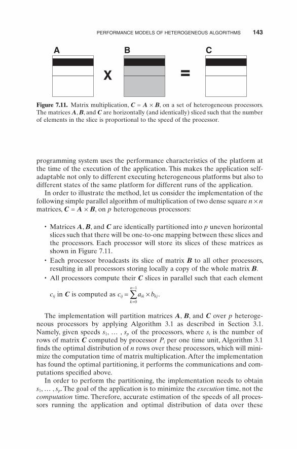
PERFORMANCE MODELS OF HETEROGENEOUS ALGORITHMS 143
programming system uses the performance characteristics of the platform at the time of the execution of the application. This makes the application self - adaptable not only to different executing heterogeneous platforms but also to different states of the same platform for different runs of the application.
In order to illustrate the method, let us consider the implementation of the following simple parallel algorithm of multiplication of two dense square n × n matrices, C = A × B , on p heterogeneous processors:
• Matrices A , B , and C are identically partitioned into p uneven horizontal slices such that there will be one - to - one mapping between these slices and the processors. Each processor will store its slices of these matrices as shown in Figure 7.11 .
• Each processor broadcasts its slice of matrix B to all other processors, resulting in all processors storing locally a copy of the whole matrix B .
• All processors compute their C slices in parallel such that each element
c ij in C is computed as c a bij ik kj
k
n
= ×=
−
∑0
1
.
The implementation will partition matrices A , B , and C over p heteroge-neous processors by applying Algorithm 3.1 as described in Section 3.1 . Namely, given speeds s 1 , … , s p of the processors, where s i is the number of rows of matrix C computed by processor P i per one time unit, Algorithm 3.1 fi nds the optimal distribution of n rows over these processors, which will mini-mize the computation time of matrix multiplication. After the implementation has found the optimal partitioning, it performs the communications and com-putations specifi ed above.
In order to perform the partitioning, the implementation needs to obtain s 1 , … , s p . The goal of the application is to minimize the execution time, not the computation time. Therefore, accurate estimation of the speeds of all proces-sors running the application and optimal distribution of data over these
A B
X
C
Figure 7.11. Matrix multiplication, C = A × B , on a set of heterogeneous processors. The matrices A , B , and C are horizontally (and identically) sliced such that the number of elements in the slice is proportional to the speed of the processor.

144 IMPLEMENTATION ISSUES
processors are not enough as it will minimize the computation time, not the execution time of the application, which also includes the communication time. The application has to also fi nd the optimal subset of the processors, minimiz-ing the execution time. Let us assume, for simplicity, that our target heteroge-neous platforms have a homogeneous communication layer. Then, the optimal subset will always consist of the fastest processors. Thus, given the problem size n and the total number q of available processors, the application can fi nd the optimal number p of the involved processors and their speeds s 1 , … , s p as follows:
• Use the benchmark code multiplying one n - element row and a dense n × n matrix to estimate the speeds s 1 , … , s q of the processors.
• Rearrange the processors such that s 1 ≥ s 2 ≥ … ≥ s q . • Given t 0 = ∞ , for i = 1 until i ≤ q , do the following:
� Estimate the execution time t i of the application given the matrices are optimally partitioned over processors P 1 , … , P i .
� If t i < t i − 1 then i = i + 1 and continue else p = i and stop.
The code performing this procedure can be easily implemented in mpC or HeteroMPI (we will use mpC in this section). First of all, the performance model of the heterogeneous algorithm of matrix multiplication is described as follows:
algorithm AxB( int p, int n, int d[p])
{
coord I=p;
node { I > =0: bench * (d[I]); }; link (J=p) { I!=J: length ( double ) * (d[I] * n) [J] - > [I]; };
};
The fi rst line of this description introduces the name A × B of the algorithvm and its three parameters: two scalar parameters p and n , and a p - element vector parameter d . We assume the following semantics of the parameters:
• p is the number of abstract processors performing the algorithm, • n is the matrix size, and • d [ i ] is the number of rows in the horizontal matrix slice allocated to the
i - th abstract processor.
The coord declaration specifi es the arrangement (one - dimensional in this case) of the abstract processors performing the algorithm.
The node declaration specifi es that the i - th processor will perform d [ i ] computation units during the execution of the algorithm. A computation unit

PERFORMANCE MODELS OF HETEROGENEOUS ALGORITHMS 145
should be the same as the one used to estimate the speed of the processors, namely, multiplication of one n - element row and a dense n × n matrix. Obviously, given the amount of computations to be performed by the proces-sor and an accurate estimation of its speed, both expressed in the same com-putation units, the programming system can easily estimate its computation time.
The link declaration specifi es the total amount of data that will be sent from each processor j to each other processor i ( i ≠ j ) during the execution of the algorithm. Obviously, given this information and performance characteristics of the network (such as latency and bandwidth), the programming system can estimate the total time of communication between every ordered pair of processors.
Given the above description of the algorithm, the rest of relevant code will look as follows:
// Run a benchmark code in parallel by all// physical processors to refresh the estimation of their speeds
{
repl double * row, * matrix, * result;
//memory allocation for row, matrix, and result
//initialization of row, matrix, and result
…
recon RowxMatrix(row, matrix, result, n);
}
// Get the total number of physical processors
q = MPC_Get_number_of_processors();
speeds = calloc(q, sizeof(double));
d = calloc(q, sizeof(int));
// Get the speed of the physical processors
MPC_Get_processors_info(NULL, speeds);
// Sort the speeds in descending order
qsort(speeds+1, q - 1, sizeof ( double ), compar);
// Calculate the optimal number of physical processors
[ host ]:
{
int p;
struct { int p; double t;} min;
double t;
min.p = 0;
min.t = DBL_MAX;
for (p=1; p < =q; p++) {
// Calculate the size of C slice to be computed by
// each of p involved physical processors

146 IMPLEMENTATION ISSUES
Partition(p, speeds, d, n); // Estimate the execution time of matrix - matrix // multiplication on m physical processors t = timeof ( algorithm AxB(p, n, d)); if (t < min.t) { min.p = p; min.t = t; } } p = min.p; }
The recon statement updates the estimate of the speed of physical proces-sors by using a serial multiplication of an n - element row and an n × n matrix with function SerialAxB . The estimated speeds are then returned in the array speeds by function MPC_Get_processors_info and reordered in the decreasing order. This newly ordered array of speeds is then used in the following code, which fi nds the optimal number of processors. Namely, it is used by the func-tion Partition performing the optimal matrix partitioning. The operator timeof uses the actual performance characteristics of the executing platform, such as the processors ’ speeds obtained by the most recent execution of the recon statement and the latency and bandwidth of the communication links, to esti-mate the execution time of the parallel algorithm A × B for specifi ed values of its parameters. Thus, after execution of this code, the value of variable p will be equal to the very optimal number of processors.
Our description of the algorithm A × B says nothing about exactly how parallel processors are interacting during execution of the algorithm. There-fore, the operator timeof must make some assumptions about the interaction in order to calculate the execution time of the algorithm. Namely, to calculate the execution time it assumes that
• the processors execute all the communications in parallel, • each processor executes all its computations in parallel with other proces-
sors, and • a synchronization barrier exists between the execution of the computa-
tions and the communications.
This assumption is satisfactory for our algorithm of matrix multiplication. At the same time, in many parallel algorithms, there are data dependencies between computations performed by different processors. One processor may need data computed by other processors in order to start its computations. This serializes some computations performed by different parallel processors. As a result, the real execution time of the algorithm will be longer than the execution time calculated proceeding from the assumption about strictly par-allel execution of computations.
On the other hand, some parallel algorithms are trying to overlap computa-tions and communications to achieve better performance. The real execution time of those algorithms will be shorter than the execution time calculated

IMPLEMENTATION OF HOMOGENEOUS ALGORITHMS 147
proceeding from the assumption that computations and communications do not overlap.
Thus, when the calculation of the execution time of different parallel algo-rithms is based on the same scenario of interaction of parallel processors during the execution of the algorithm, the calculated execution time may be not accurate.
The mpC language addresses the problem. It allows the programmer to include the scenario of interaction of parallel processes during the execution of the parallel algorithm into the description of its performance model. This and other features of the mpC language are presented in detail in Chapter 8 .
7.4 IMPLEMENTATION OF HOMOGENEOUS ALGORITHMS FOR HETEROGENEOUS PLATFORMS
As discussed in Section 7.1 , the design and implementation of original hetero-geneous algorithms is not the only approach to high - performance computing on heterogeneous platforms. Another approach consists in the effi cient imple-mentation of traditional homogeneous parallel algorithms. This approach, originally proposed in Kalinov and Lastovetsky (1999b) for the acceleration of ScaLAPACK applications on heterogeneous platforms, is based on a multiple - processes - per - processor confi guration of the application implement-ing the homogeneous algorithm. While all processes are supposed to perform the same amount of computations, the load of the heterogeneous processors is balanced by the heterogeneous distribution of the parallel processes over the processors. This approach is known as HeHo , He terogeneous distribution of processes of the processors and Ho mogeneous distribution of data between the processes, in contrast to the HoHe approach, Ho mogeneous distribution of processes (one process per processor) and He terogeneous distribution of data between the processes (Kalinov and Lastovetsky, 2001 ).
The main problem of the HeHo approach is to fi nd the optimal confi gura-tion of the application, namely,
• the optimal subset of the heterogeneous processors to be involved in the execution of the algorithm and
• the optimal distribution of processes over the processors as well as the optimal values of other algorithmic parameters.
This problem has been addressed in a number of research papers (Kalinov and Lastovetsky 1999b ; Kalinov and Lastovetsky 2001 ; Kishimoto and Ichi-kawa 2004 ; Kalinov and Klimov 2005 ; Cuenca, Gim é nez, and Martinez, 2005 ; Reddy and Lastovetsky, 2006 ). In Kishimoto and Ichikawa (2004) , a simple performance model of the target heterogeneous cluster is fi rst built for the given parallel application from a large number of experimental runs of differ-ent confi gurations of the application. Then this performance model is used to

148 IMPLEMENTATION ISSUES
fi nd the optimal subset of the processors of the cluster and the optimal distri-bution of processes over the processors for that application on this cluster.
In Kalinov and Klimov (2005) , the performance of a processor involved in the execution of the given application is represented by a function of the number of processes running on the processor and the amount of data distrib-uted to the processor. A simple algorithm that fi nds the optimal number of processes and their optimal distribution over the processors based on this model is proposed.
The implementation of parallel dynamic programming algorithms for het-erogeneous platforms is studied in Cuenca, Gim é nez, and Martinez (2005) . It proposes heuristic algorithms for the estimation of the optimal confi guration of applications implementing such algorithms.
In Reddy and Lastovetsky (2006) , the mpC/HeteroMPI approach based on the specifi cation of the performance model of the parallel algorithm is applied to a self - adaptable implementation of Parallel Basic Linear Algebra Subpro-grams (PBLAS) (Choi et al ., 1996b ). The accurate estimation of platform parameters, optimization of algorithmic parameters (including the number of parallel processes and their arrangement), and optimal mapping of processes to the heterogeneous processors are performed automatically by the program-ming system based on the specifi cation of the implemented homogeneous algorithm provided by the application programmer.