High order numerical methods for highly oscillatory...

Mathematical Modelling and Numerical Analysis Will be set by the publisherModelisation Mathematique et Analyse Numerique

HIGH ORDER NUMERICAL METHODS FOR HIGHLY OSCILLATORY PROBLEMS ∗

DAVID COHEN 1 AND JULIA SCHWEITZER 2

Abstract. This paper is concerned with the numerical solution of nonlinear Hamiltonian oscillatory systems ofsecond-order differential equations of a special form. We present numerical methods of high asymptotic as wellas time stepping order based on the modulated Fourier expansion of the exact solution. Furthermore, numericalexperiments on the modified Fermi-Pasta-Ulam problem support our investigations.

1991 Mathematics Subject Classification. 34E05 and 34E13 and 65L20 and 65P10.

March 4, 2014.

1. INTRODUCTION

We consider the numerical discretisation of second-order Hamiltonian differential equations with highly oscillatorysolutions of the special form

x+Ω2x = g(x) :=−∇U(x) , (1)with the square block matrix

Ω =

(0 00 ωI

), with ω ≫ 1 ,

and a smooth nonlinear potential U . This is a Hamiltonian problem with

H(x, x) = 12∥x∥2 +

12∥Ωx∥2 +U(x) . (2)

For the above problem, we will only consider initial values satisfying the bounded energy assumption

12∥x(0)∥2 +

12∥Ωx(0)∥2 ≤ E (3)

with a constant E independent of the large parameter ω .We decompose the solution x = (x1,x2) and the nonlinearity g(x) = (g1(x),g2(x)) according to the blocks of the matrix

Ω. One thus has a solution with a slowly varying component x1 and a rapidly varying one x2.

Keywords and phrases: Highly oscillatory differential equations and Multiple time scales and Fermi-Pasta-Ulam problem and Modulated Fourierexpansions and High-order numerical schemes and Adiabatic invariants∗ This research is supported by the Lars Hierta Memorial Foundation and by the Deutsche Forschungsgemeinschaft via GRK 1294.1 Matematik och matematisk statistik, Umea universitet, 90187 Umea, Sweden.e-mail: [email protected] Institut fur Angewandte und Numerische Mathematik, Karlsruher Institut fur Technologie, 76128 Karlsruhe, Germany.e-mail: [email protected]

c⃝ EDP Sciences, SMAI 1999

2 TITLE WILL BE SET BY THE PUBLISHER

Due to the presence of fast and slow time scales the numerical discretisation of problems of the form (1) is a difficulttask. One of the most efficient integrators for this kind of highly-oscillatory problems are the trigonometric integrators,see for example the review [7], [17] and [15, Chapter XIII] as well as references therein. Other type of numerical schemeswere also proposed in the literature. Let us mention (without being exhaustive) the following works: the methods based onaveraging techniques from [2], see also [3]; the numerical schemes based on homogenisation from [18]; the multi-scalemethods from [21]; the IMEX method from [20], see also the preprint [19]; and more recently the energy-preservingschemes from [22]. The order of convergence in the time stepsize of these numerical integrators is at most two. Themain motivation of the present work is to present and analyse numerical methods for problems (1) of higher order ofconvergence independent of the frequency.

For the numerical discretisation of (1), we will use a modulated Fourier expansion (MFE), see [14] and [5]. Thisanalytical tool basically decomposes the exact solution of our problem into a slowly varying part and into oscillatoryparts. The first terms of this expansion were already used in [4] to develop efficient geometric numerical integrators for(1). In particular, symmetric and reversible methods based on the MFE were presented in [4] together with their energy-conservation properties on longtime intervals. However, the order of the methods proposed in [4] was not examined andextensions of these methods to higher-order numerical schemes remain to be investigated. This is the main objective ofthe present paper. At this point, it should be noted that one drawback of the proposed approach is the fact that it mayprove difficult to generalise it to more complicated situations.

Much in the same spirit as the present work is the series of papers [8–10] on asymptotic-numerical solvers for differen-tial equations with highly oscillatory coefficients. In these references, the special structure (a MFE in fact) of the forcingterm present in the problem permits to derive efficient numerical methods. Furthermore, the results from the recent ref-erence [1] are also closely related to the type of problems (1) and to the numerical schemes that we propose. The majordifference is that the work [1] deals with highly oscillatory equations with a small parameter in the nonrelativistic regime.Let us finally mention the recent work [11] which also uses the first terms of a MFE to derive numerical schemes for theKlein-Gordon equation in the nonrelativistic limit regime.

The paper is organised as follows. After recalling some results on the MFE in Section 2, we will describe the construc-tion of the numerical schemes based on the first terms of the modulated Fourier expansion following the lines of [15, Sec-tion XIII.3.1] and [4, Chapter 3] in Section 3. In the forth section, we will derive numerical schemes of order one, two,three and four for (1). In the last section we present numerical experiments on the modified Fermi-Pasta-Ulam problem

2. PREPARATORY RESULTS AND BUILDING-BLOCKS FOR HIGH-ORDER NUMERICAL SCHEMES

We present two fundamental results from [15, Chapter XIII] and [5] that we need in order to derive high-order numericalschemes for (1). First, let us recall the following result on the modulated Fourier expansion of the exact solution of (1).

Theorem 2.1 (Theorem XIII.5.1 of [15]). Consider a solution x(t) of (1) which satisfies the bounded-energy condition(3) and stays in a compact set K for 0 ≤ t ≤ T . Then, the solution admits an expansion

x(t) = y(t)+ ∑0<|k|<N

eikωtzk(t)+RN(t)

for arbitrary N ≥ 2, where the remainder term and its derivative are bounded by

RN(t) = O(ω−N) and RN(t) = O(ω−N) for 0 ≤ t ≤ T .

(Remark that one can get slightly sharper bounds for the remainder terms, see the end of the proof of [15, Theo-rem XIII.5.1] for details). The real-valued functions y = (y1,y2) and the complex-valued functions zk = (zk

1,zk2) together

with all their derivatives (up to arbitrary order M) are bounded by

y1 = O(1) , z11 = O(ω−3) , zk = O(ω−k−2) ,

y2 = O(ω−2) , z12 = O(ω−1) ,

TITLE WILL BE SET BY THE PUBLISHER 3

for k = 2, . . . ,N −1. Moreover z−k = zk for all k. The constants symbolised by the O-notation are independent of ω and twith 0 ≤ t ≤ T . Finally, the asymptotic expansion

x⋆(t) := y(t)+ ∑0<|k|<N

eikωtzk(t) (4)

is called the (truncated) modulated Fourier expansion of the exact solution.

In order to find the modulation functions y(t) and zk(t), one inserts the expansion (4) into the differential equation(1), expands the nonlinearity g(x) around the smooth part (y1(t),0) and compares the coefficients in front of eikωt . Thisyields a system of nonstiff differential equations for y1(t) and z1

2(t) and algebraic relations for the rest of the modulationfunctions.

As explained in the proof of Theorem XIII.5.1 in [15], the functions y1(t) and z12(t) are given by differential equations

of the formy1 = ∑

l≥0ω−lF1l(y1, y1,z1

2) , z12 = ∑

l≥1ω−lF2l(y1, y1,z1

2) , (5)

and the remaining modulation functions by algebraic relations

zki = ∑

l≥0ω−lGk

il(y1, y1,z12) . (6)

Observe that y2 = z02, and that z−k

i is the complex conjugate of zki , so that also G−k

il is the complex conjugate of Gkil . For an

efficient computation of the functions Fil and Gkil , we rely on the recurrence relations given by the following

Lemma 2.2 (Lemma 2.1 of [5]). The functions Fil and Gkil defining the nonstiff differential equations (5) and algebraic

equations (6) satisfy the recurrence relations (for l ≥ 0):

F1l = S1(0, l) , Gk1l =

1k2

(∑

m+n+ j=l−2LmLnGk

1 j +2ik ∑m+ j=l−1

LmGk1 j −S1(k, l −2)

),

F2l =12i

(S2(1, l −1)− ∑

m+ j=l−1LmF2 j

), Gk

2l =1

k2 −1

(∑

m+n+ j=l−2LmLnGk

2 j +2ik ∑m+ j=l−1

LmGk2 j −S2(k, l −2)

).

The sums are over m ≥ 0,n ≥ 0, j ≥ 0, and we have used the abbreviation

Si(k, l) = ∑m,n≥0

1m!n! ∑

α,βs(α)+s(β )=k

∑e, f

s(e)+s( f )=l

Dm1 Dn

2gi(y1,0)(Gα1e,G

β2 f ) .

Here, α = (α1, . . . ,αm), β = (β1, . . . ,βn), e = (e1, . . . ,em) as well as f = ( f1, . . . , fn) are multi-indices with αi = 0, βi

arbitrary, ei ≥ 0, fi ≥ 0, and (Gα1e,G

β2 f ) = (Gα1

1,e1, . . . ,Gαm

1,em,Gβ1

2, f1, . . . ,Gβn

2, fn). We use the abbreviation s(α) = ∑mi=1 αi and

similarly for the other multi-indices. Furthermore, the operator Ll applied to a smooth function G(y1, y1,z2) is definedby

LlG = D2G ·F1l + D3G ·F2l +

D1G · y1 if l = 00 if l ≥ 1 ,

where l ≥ 0 and D j denotes the partial derivative with respect to the jth argument of G(y1, y1,z2). Finally, we note that

Gk10 = 0 , Gk

11 = 0 for k = 0 ,

Gk20 = 0 , Gk

21 = 0 for k =±1 ,

G±120 = z±1

2 , G±12l = 0 for l ≥ 1 .


3. GENERAL CONSTRUCTION OF THE NUMERICAL METHODS AND SOME RESULTS

We propose to solve the truncated nonstiff system of differential equations for the modulation functions y1 and z12 up to

asymptotic order N using a standard numerical time stepping scheme, such as an explicit Runge-Kutta method of highertime stepping order p with a (possibly) large time stepsize. To obtain an approximation to the solution of the originalhighly oscillatory problem (1), we insert the numerical approximations of y1 and z1

2 into the algebraic equations for theremaining modulation functions and compute the truncated MFE (4) of asymptotic order N.

To summarise, we obtain a numerical integrator of asymptotic order N and time stepping order p for (1) following theflow chart

(1) Truncate the ansatz (5) and (6) after the O(ω−N)-terms.(2) Use the recurrence relations given by the above lemma up to terms of asymptotic order O(ω−N).(3) Solve numerically the nonstiff truncated differential equations (5) with an explicit scheme of high time stepping

order p(4) Compute the algebraic relations (6) and the approximation of the solution of (1) using the MFE (4).

We would like to point out, that the initial values y1(0), y1(0) and z12(0) for the differential equations (5) are obtained from

the conditions

x⋆(0) = x(0) and x⋆(0) = x(0) .

This yields a nonlinear system of equations, which can be solved by a fixed point iteration as shown in [15, ChapterXIII.3].

Note, that step (4) of the flow chart is to be understood as a postprocessing, which only needs to be performed at times,where the solution of the original problem is required. The size of the new system is smaller than that of the originalone. Therefore, in terms of storage the method is comparable to other methods applied directly to the original system.However, the right hand side of the new system is more complicated depending on the nonlinearity and the asymptoticorder. If the nonlinear interaction is nonlocal, the computational cost may grow considerably. It approximately scaleswith the largest number of directly interacting variables via the nonlinearity to the power of the asymptotic order timesthe number of all variables, since the derivatives of the nonlinearity appearing in the equations for the truncated systemyield multilinear forms of the respective order.

We have the following error estimates on compact time intervals for the proposed numerical approximations of solu-tions to problem (1).

Proposition 3.1. Under the assumptions of Theorem 2.1, if we solve the truncated system for the modulation functions ofasymptotic order N with a numerical time stepping scheme of order p, then the error of the approximation satisfies

∥x(tn)− yn − ∑0<|k|<N

eikωtnzkn∥ ≤Caω−N +Cthp .

In addition, the approximation of the time derivative of the solution satisfies

∥x(tn)− yn − ∑0<|k|<N

(ikωzkn + zk

n)eikωtn∥ ≤ Caω−N +Cthp ,

where the approximation to z12,n is obtained by the differential equation for z1

2 and the approximations to the remainingmodulation functions are computed by differentiation of the algebraic relations.

Proof. For the proof of the error bound of the solution itself, we insert the exact truncated MFE and use the triangleinequality to obtain

∥x(tn)− yn − ∑0<|k|<N

zkneikωtn∥ ≤ ∥x(tn)− x⋆(tn)∥+∥y(tn)+ ∑

0<|k|<Nzk(tn)eikωtn − yn − ∑

0<|k|<Nzk

neikωtn∥ .


The first term yields the asymptotic part of the error by Theorem 2.1. For y1 and z12 the numerical time stepping scheme

of order p yields approximations y1,n and z12,n satisfying y1(tn)− y1,n = O(hp) as well as z1

2(tn)− z12,n = O(hp). For

a sufficiently smooth function g the error of the approximation to the remaining modulation functions is then at mostO(hp). This yields the stated error bound.

For the error of the derivative of the solution, we obtain

∥x(tn)− yn − ∑0<|k|<N

(ikωzkn + zk

n)eikωtn∥

≤ ∥x(tn)− x⋆(tn)∥+∥y(tn)+ ∑0<|k|<N

(ikωzk(tn)+ zk(tn))eikωtn − yn − ∑0<|k|<N

(ikωzkn + zk

n)eikωtn∥ .

To treat the term ikω(zk(tn)− zkn), we observe that the modulation functions obtained by the algebraic relations are of the

form ω−k times functions of at most order one evaluated at the numerical solutions of the MFE. This therefore cancelsthe factor of ω and only the error of the time stepping scheme remains. The remaining terms are treated similarly as inthe first part of the proof.

Let us further mention that the proposed numerical methods do not suffer from numerical resonances (when the productof the stepsize and the large frequency ω is close to a nonzero integer multiple of π). Furthermore, the proposed schemes(of asymptotic order greater than one) correctly model the slow energy exchange in the problem, since the evolution ofz1

2, which describes this slow exchange of energy, is present in our numerical approximation given by the truncated MFE(4). This will be illustrated in the numerical experiments presented in Subsection 5.3.

Finally, as demonstrated in [4], by carefully selecting the numerical integrators for the time integration of the nonstiffsystem (5), one can obtain longtime energy-conservation properties of the numerical solutions using the proposed ap-proach. Such a result for generic integrators is not in the scope of the present work. But, one can still observe excellentlongtime energy-conservation, even in this case, in the numerical experiments presented below.

4. HIGH-ORDER NUMERICAL METHODS

This section presents the nonstiff systems together with their algebraic relations and the corresponding truncated MFEup to asymptotic order four approximating highly oscillatory problems of the form (1). The derivation directly followsfrom Lemma 2.2 but is rather tedious, thus we only present the results. Throughout the remainder of the section we usethe abbreviation gi := gi(y1,0) for i = 1,2 for the sake of presentation.

4.1. System of asymptotic order one

In order to obtain an asymptotic approximation of order one for problems of the form (1), one needs to solve thenonstiff system

y1 = g1

and compute the truncated MFE

x⋆(t) :=(y1(t),0

).

In this case, there are no algebraic relations needed yet. Note, that Theorem 2.1 actually only holds for N ≥ 2. However,we included this system for the sake of completeness. It will be shown later, that the scaling in ω holds, but the solutiondoes not show the proper energy conservation properties.


4.2. System of asymptotic order two

In order to obtain an asymptotic approximation of order two for problems of the form (1), one needs to solve thenonstiff system

y1 = g1 +D22g1(z1

2,z−12 )+ω−2D2g1g2 ,

z12 =

ω−1

2iD2g2z1

2 ,

insert the solution into the algebraic relations

y2 = z02 = ω−2g2 ,

z11 = 0 ,

and with this, compute the truncated MFE

x⋆(t) := y(t)+ eiωtz1(t)+ e−iωt z1(t) .

4.3. System of asymptotic order three

In order to obtain an asymptotic approximation of order three for problems of the form (1), one needs to solve thenonstiff system

y1 = g1 +D22g1(z1

2,z−12 )+ω−2D2g1g2 ,

z12 =

ω−1

2iD2g2z1

2 +ω−2

4D1D2g2

(y1,z1

2),


y2 = z02 = ω−2g2 ,

z11 =−ω−2D2g1z1

2 ,


x⋆(t) := y(t)+ eiωtz1(t)+ e−iωt z1(t) . (11)

4.4. System of asymptotic order four

Finally, in order to obtain an asymptotic approximation of order four for problems of the form (1), one needs to solvethe nonstiff system

y1 = g1 +D22g1(z1

2,z−12 )+ω−2D2g1g2 +

14

D42g1(z1

2,z12,z

−12 ,z−1

2 )

+ω−2

D2g1D22g2(z1

2,z−12 )+D3

2g1(z12,z

−12 ,g2)−2ReD1D2g1

(D2g1z−1

2 ,z12)

+ω−4

D2g1(D2g2g2 −D1g2g1 −D2

1g2(y1, y1))+

12

D22g1(g2(y2,0),g2)

,

z12 =

ω−1

2iD2g2z1

2 +ω−2

4D1D2g2

(y1,z1

2)+

ω−1

4iD3

2g2(z12,z

12,z

−12 )

+ω−3

2i

−D1g2D2g1z1

2 +D22g2

(z1

2,g2)− 1

4D1D2g2

(g1,z1

2)− 1

4D2

1D2g2(y1, y1,z1

2)+

14

D2g2(D2g2z1

2)

,



y2 = z02 = ω−2g2 +ω−2D2

2g2(z12,z

12) ,

z11 =−ω−2D2g1z1

2 −2iω−3D1D2g1(y1,z12) ,

z21 =−ω−2

8D2

2g1(z12,z

12) ,

z22 =−ω−2

6D2

2g2(z12,z

12) ,


x⋆(t) := y(t)+ eiωtz1(t)+ e−iωt z1(t)+ e2iωtz2(t)+ e−2iωt z2(t) . (14)

5. NUMERICAL EXPERIMENTS

We conclude this paper with numerical experiments on the modified Fermi-Pasta-Ulam problem in order to illustratethe accuracy as well as the energy conservation properties of the proposed integrators.

5.1. The modified Fermi-Pasta-Ulam problem

Let us consider the modified Fermi-Pasta-Ulam problem, as described in [15, Section I.5.1], i.e. with Hamiltonian

H(p1, p2,q1,q2) =12

3

∑i=1

(p21,i + p2

2,i)+ω2

2

3

∑i=1

q22,i +U(q1,q2) ,

where

U(q1,q2) =14

(q1,1 −q2,1)

4 +2

∑i=1

(q1,i+1 −q2,i+1 −q1,i −q2,i)4 +(q1,3 +q2,3)

4.

The total energy H is exactly conserved and this problem also possesses an almost-invariant, namely the oscillatory energy

I(p2,q2) =12

3

∑i=1

p22,i +

ω2

2

3

∑i=1

q22,i .

Indeed, this quantity is nearly preserved over times that are exponentially long in the high frequency ω along the exactsolution of the modified Fermi-Pasta-Ulam problem [5]. The initial values for the second order differential equation (1)(using the notations q = (q1,q2) = (x1,x2) = x and similarly for the momenta p) obtained with the above Hamiltonianfunction are given by

q1,1(0) = 1 , p1,1(0) = 1 , q2,1(0) = 1/ω , p2,1(0) = 1

and zero for the remaining ones. These initial values satisfy the bounded energy assumption (3).

5.2. Numerical study of the asymptotic and time stepping order

In oder to demonstrate the behaviour of the error of our numerical method, we exemplary consider the system (11) ofasymptotic order N = 3 for the modified Fermi-Pasta-Ulam problem and solve it with an explicit Runge-Kutta methodof time stepping order p = 3. For different values of ω we compute the solution up to time Tend = 1 for varying timestepsizes h and measure the relative errors at Tend using a high resolution simulation of the original system (1) solved withthe Stormer-Verlet scheme as reference solution. In the left part of Figure 1, the error is plotted versus the time stepsize h.It shows third order convergence in the time stepsize up to the point, where the asymptotic error dominates. Note that the


10−3 10−2 10−1 10010−6

10−5

10−4

10−3

10−2

10−1

h

error

h3

101 101.5 10210−6

10−5

10−4

10−3

10−2

10−1

ω

error

ω−3

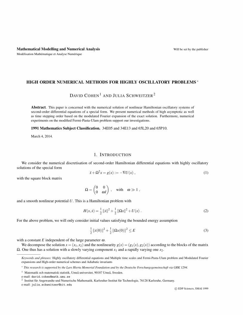
FIGURE 1. The error of the numerical approximation using the terms of the MFE up to asymptoticorder N = 3 solved with a Runge-Kutta scheme of time stepping order p = 3 for the modified Fermi-Pasta-Ulam problem is plotted versus the time stepsize (left) and the parameter ω (right). The referencelines have slope 3. In the left picture, the different lines correspond to different values of ω growingfrom top to bottom.

error curves are almost identical for the different values of ω before the saturation occurs. Therefore, the pre-asymptoticconvergence in the time stepsize is indeed independent of ω . In the right part of Figure 1 the error is plotted against thevalues of ω always computed with time stepsizes small enough, that the error is dominated by the asymptotic part. Weagain observe the predicted scaling in ω−1.

5.3. Numerical study of the energy conservation

Next, we use the numerical approximations to the solution x⋆(t) of the truncated systems of asymptotic order N fromone to four to compute the total energy H−0.8 (for a better display), the oscillatory energy I together with its componentson the time interval [0,100] for a fixed (large) time stepsize h = 10−2. The nonstiff differential equations are all solvedwith an explicit Runge-Kutta scheme of time stepping order p = 3. The results are shown in Figure 2 along with theenergies computed by the Stormer-Verlet method applied to the original system (1) with a small stepsize h = 10−4. Onecan observe that the modelling of the exchange of energy gets better by increasing the number of modulation functionspresent in the method, namely the asymptotic order N.

A numerical experiment with the same parameters as above but on a much longer time interval [0,10000] is presented inFigure 3. Excellent energy preservation is observed for the numerical solution of the truncated system (14) of asymptoticorder N = 4 solved with an explicit Runge-Kutta method of time stepping order p = 4.

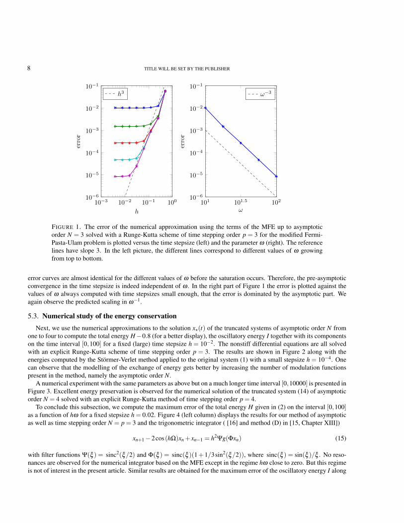
To conclude this subsection, we compute the maximum error of the total energy H given in (2) on the interval [0,100]as a function of hω for a fixed stepsize h = 0.02. Figure 4 (left column) displays the results for our method of asymptoticas well as time stepping order N = p = 3 and the trigonometric integrator ( [16] and method (D) in [15, Chapter XIII])

xn+1 −2cos(hΩ)xn + xn−1 = h2Ψg(Φxn) (15)

with filter functions Ψ(ξ ) = sinc2(ξ/2) and Φ(ξ ) = sinc(ξ )(1+1/3sin2(ξ/2)), where sinc(ξ ) = sin(ξ )/ξ . No reso-nances are observed for the numerical integrator based on the MFE except in the regime hω close to zero. But this regimeis not of interest in the present article. Similar results are obtained for the maximum error of the oscillatory energy I along


0 10 20 30 40 50 60 70 80 90 1000

0.2

0.4

0.6

0.8

1

1.2

1.4

MFE with N = 1 and p = 4

0 10 20 30 40 50 60 70 80 90 1000

0.2

0.4

0.6

0.8

1

1.2

1.4


0 10 20 30 40 50 60 70 80 90 1000

0.2

0.4

0.6

0.8

1

1.2

1.4


0 10 20 30 40 50 60 70 80 90 1000

0.2

0.4

0.6

0.8

1

1.2

1.4


0 10 20 30 40 50 60 70 80 90 1000

0.2

0.4

0.6

0.8

1

1.2

1.4

Stormer-Verlet method

FIGURE 2. Exchange of energy between stiff springs for the modified Fermi-Pasta-Ulam problemsolved using the MFE with different asymptotic orders and the Stormer-Verlet method. Blue: totalenergy H −0.8. Red: oscillatory energy I. Shades of green: components of oscillatory energy Ii.

0 2500 5000 75000

0.2

0.4

0.6

0.8

1

1.2

1.4

Long time simulation for MFE with N = 4 and p = 4

FIGURE 3. Exchange of energy between stiff springs for the modified Fermi-Pasta-Ulam problem ona long time interval solved with the method of asymptotic order N = 4 and time stepping order p = 4.Blue: total energy H − 0.8. Red: oscillatory energy I. Shades of green: components of oscillatoryenergy Ii.


numerical solutions given by the proposed methods in the left column of Figure 4. Finally, we would like to commenton the fact that particular choices of the filter functions present in (15) could also lead to trigonometric integrators thatdo not suffer from resonances in the oscillatory and/or the total energy of the problem as seen in the last two rows ofFigure 4. These plots were obtained using method (E) in [15, Chapter XIII], that is with filter functions Ψ(ξ ) = sinc2(ξ )and Φ(ξ ) = 1 and method (G) in [13], that is with filter functions Ψ(ξ ) = sinc3(ξ ) and Φ(ξ ) = sinc(ξ ). Similar resultsare also obtained with the modified trigonometric integrators presented in [19].

5.4. Runtime comparison

Finally, we show some runtime comparisons. To that end, we solve the modified Fermi-Pasta-Ulam problem withω = 500 on the time interval [0,10] with the trigonometric method (E) as well as the MFE method of asymptotic orderN = 2,3,4 using an explicit Runge-Kutta method of time stepping order p = 4. It can be seen that, for high accuracies,there is some potential in the MFE methods to beat the trigonometric methods, which is the state of the art numericalschemes for this kind of problem. From Figure 5 it can also be observed, that the method with asymptotic order N = 3is the most efficient choice, since the system to solve is hardly more complicated than the system for the method ofasymptotic order N = 2 where the latter lacks accuracy.

6. CONCLUSION AND FURTHER RESEARCH

Using a modulated Fourier expansion, we have derived high order numerical algorithms for the time discretisation ofsecond-order differential equations with highly oscillatory solutions. Furthermore, our convergence results and the mainproperties of these high order numerical methods were illustrated on the modified Fermi-Pasta-Ulam problem.

Finally, we would like to mention that the techniques presented here could be used to derive high-order numericalmethods for the discretisation of highly-oscillatory systems with multiple frequencies (as those studied in [6]) or for thenumerical discretisation of Hamiltonian PDEs (using the MFE presented in [12] for example). We will investigate thesequestions in the future.

REFERENCES

[1] W. Bao, X. Dong, and X. Zhao. Uniformly correct multiscale time integrators for highly oscillatory second order differential equations.arXiv:1212.4939, 2012.

[2] F. Castella, P. Chartier, and E. Faou. An averaging technique for highly oscillatory Hamiltonian problems. SIAM J. Numer. Anal., 47(4):2808–2837,2009.

[3] P. Chartier, A. Murua, and J. M. Sanz-Serna. Higher-order averaging, formal series and numerical integration I: B-series. Found. Comput. Math.,10(6):695–727, 2010.

[4] D. Cohen. Analysis and Numerical Treatment of Highly Oscillatory Differential Equations. PhD thesis, University of Geneva, 2004.[5] D. Cohen, E. Hairer, and Ch. Lubich. Modulated Fourier expansions of highly oscillatory differential equations. Found. Comput. Math., 3(4):327–

345, 2003.[6] D. Cohen, E. Hairer, and Ch. Lubich. Numerical energy conservation for multi-frequency oscillatory differential equations. BIT, 45:287–305, 2005.[7] D. Cohen, T. Jahnke, K. Lorenz, and Ch. Lubich. Numerical integrators for highly oscillatory Hamiltonian systems: a review. In Analysis, modeling

and simulation of multiscale problems, pages 553–576. Springer, Berlin, 2006.[8] M. Condon, A. Deano, and A. Iserles. On second-order differential equations with highly oscillatory forcing terms. Proc. R. Soc. Lond. Ser. A

Math. Phys. Eng. Sci., 466(2118):1809–1828, 2010.[9] M. Condon, A. Deano, and A. Iserles. On systems of differential equations with extrinsic oscillation. Discrete Contin. Dyn. Syst., 28(4):1345–1367,

2010.[10] M. Condon, A. Deano, and A. Iserles. Asymptotic solvers for oscillatory systems of differential equations. SeMA J., (53):79–101, 2011.[11] E. Faou and K. Schratz. Asymptotic preserving schemes for the Klein-Gordon equation in the non-relativistic limit regime. Numerische Mathe-

matik, pages 1–29, 2013.[12] L. Gauckler. Long-time analysis of Hamiltonian partial differential equations and their discretizations. PhD thesis, Universitat Tubingen, 2010.

http://nbn-resolving.de/urn:nbn:de:bsz:21-opus-47540.[13] V. Grimm and M. Hochbruck. Error analysis of exponential integrators for oscillatory second-order differential equations. J. Phys. A, 39(19):5495–

5507, 2006.[14] E. Hairer and Ch. Lubich. Long-time energy conservation of numerical methods for oscillatory differential equations. SIAM J. Numer. Anal.,

38(2):414–441 (electronic), 2000.


0 π 2π 3π 4π

0.1

0.2

hω

Energy error for MFE with N = 3, p = 3 and h = 0.02

0 π 2π 3π 4π

0.1

0.2

hω

Deviation of oscillatory energy for MFE with N = 3, p = 3 and h = 0.02

0 π 2π 3π 4π

0.1

0.2

hω

Energy error for trigonometric method (D) with h = 0.02

0 π 2π 3π 4π

0.1

0.2

hω

Deviation of oscillatory energy for trigonometric method (D) with h = 0.02

0 π 2π 3π 4π

0.1

0.2

hω

Energy error trigonometric method (E) with h = 0.02

0 π 2π 3π 4π

0.1

0.2

hω

Deviation of oscillatory energy for trigonometric method (E) with h = 0.02

0 π 2π 3π 4π

0.1

0.2

hω

Energy error for trigonometric method (G) with h = 0.02

0 π 2π 3π 4π

0.1

0.2

hω

Deviation of oscillatory energy for trigonometric method (G) with h = 0.02

FIGURE 4. Maximum error of total energy H (left) and maximum deviation of oscillatory energy I(right) on the interval [0,100] for MFE with N = p = 3 and trigonometric methods (D), (E) and (G).


10−2 10−1 100 101 10210−8

10−7

10−6

10−5

10−4

10−3

10−2

10−1

100

computing time in sec.

error

ω = 500 on the interval [0, 10]

MFE N = 2MFE N = 3MFE N = 4

trigonometric method (E)

FIGURE 5. Runtime comparison between the MFE-based methods with N = 2,3,4 and p = 4 and thetrigonometric method (E).

[15] E. Hairer, Ch. Lubich, and G. Wanner. Geometric Numerical Integration. Structure-Preserving Algorithms for Ordinary Differential Equations.Springer Series in Computational Mathematics 31. Springer, Berlin, 2002.

[16] M. Hochbruck and Ch. Lubich. A Gautschi-type method for oscillatory second-order differential equations. Numer. Math., 83(3):403–426, 1999.[17] M. Hochbruck and A. Ostermann. Exponential integrators. Acta Numerica, 19:209–286, 2010.[18] C. Le Bris and F. Legoll. Integrators for highly oscillatory Hamiltonian systems: an homogenization approach. Discrete Contin. Dyn. Syst. Ser. B,

13(2):347–373, 2010.[19] R. I. McLachlan and A. Stern. Modified trigonometric integrators. arXiv:1305.3216, 2013.[20] A. Stern and E. Grinspun. Implicit-explicit variational integration of highly oscillatory problems. Multiscale Model. Simul., 7(4):1779–1794, 2009.[21] M. Tao, H. Owhadi, and J. E. Marsden. Nonintrusive and structure preserving multiscale integration of stiff ODEs, SDEs, and Hamiltonian systems

with hidden slow dynamics via flow averaging. Multiscale Model. Simul., 8(4):1269–1324, 2010.[22] B. Wang and X. Wu. A new high precision energy-preserving integrator for system of oscillatory second-order differential equations. Phys. Lett.

A, 376(14):1185–1190, 2012.

High order numerical methods for highly oscillatory...

Documents

Transcript of High order numerical methods for highly oscillatory...