High Harmonic Generation in HollowCore Waveguides

Aaron von Conta

Master’s Thesis

Faculty of EngineeringDepartment of Physics

2012

I

Anything worth doing, is worth doing rightHunter S. Thompson

II

III

Abstract

The main goal of this thesis is to initiate a set of experiments on high-order harmonicgeneration (HHG) in hollow core waveguides and to verify a higher conversion efficiency ofHHG in waveguides compared to classical HHG schemes.

High harmonics are in this context electromagnetic waves generated by focusing laser lightinto a dilute noble gas. The frequency of the thereby generated waves is q times largerthan the frequency of the driving laser. Compared to second harmonic generation or thirdharmonic generation where q is 2 and 3, q in case of HHG can theoretically be up to ahundred or more. The obtained radiation, which is in the vacuum ultraviolet (VUV) andextreme ultraviolet (XUV) spectral regions, has a set of interesting properties which makeit valuable for attosecond physics, classical spectroscopy and many more fields of physics.

Classically, a so-called free focusing geometry is used to generate high harmonics. Thisrepresents schematically just focusing the laser beam into a gas jet. Due to the absorptionlength of the harmonics at atmospheric pressure the whole setup, from generation, tointeraction, to detection must be placed in vacuum. Using hollow core waveguides for thegeneration process results theoretically in a higher generation efficiency and better gasconfinement in vacuum environment, therefore a higher conversion efficiency is expected.

Within this thesis a general theoretical foundation will be laid to understand the process ofhigh harmonic generation and to explain the advantages of using hollow core waveguides.To underline the theoretical claims, a set of experiments is planned. The current status ofthe experiments is presented.

IV

Contents

1 Introduction 11.1 Prologue . . . . . . . . . . . . . . . . . . . . . . . . . . . . . . . . . . . . . . . 11.2 A Phenomenological Picture . . . . . . . . . . . . . . . . . . . . . . . . . . . . 2

1.2.1 What is HHG . . . . . . . . . . . . . . . . . . . . . . . . . . . . . . . . 21.2.2 Experimental considerations . . . . . . . . . . . . . . . . . . . . . . . . 2

1.3 The Process of HHG in Gases . . . . . . . . . . . . . . . . . . . . . . . . . . . 21.3.1 The three step model . . . . . . . . . . . . . . . . . . . . . . . . . . . 21.3.2 Simulations based on the three step model . . . . . . . . . . . . . . . . 31.3.3 Shortcomings of the presented picture . . . . . . . . . . . . . . . . . . 4

1.4 Introduction to Nonlinear Optics . . . . . . . . . . . . . . . . . . . . . . . . . 51.4.1 Waves and harmonics . . . . . . . . . . . . . . . . . . . . . . . . . . . 51.4.2 The transition from linear to nonlinear optics . . . . . . . . . . . . . . 61.4.3 Nonlinear optics . . . . . . . . . . . . . . . . . . . . . . . . . . . . . . 7

1.5 Light Propagation in Waveguides . . . . . . . . . . . . . . . . . . . . . . . . . 71.5.1 Properties of simple waveguides . . . . . . . . . . . . . . . . . . . . . . 71.5.2 Dealing with more complicated structures . . . . . . . . . . . . . . . . 8

1.6 Scope and Outline of this Work . . . . . . . . . . . . . . . . . . . . . . . . . . 8

2 Single-Atom Response 102.1 Introduction to the Atomic Polarization . . . . . . . . . . . . . . . . . . . . . 102.2 Modeling the Electron Wave function . . . . . . . . . . . . . . . . . . . . . . . 11

2.2.1 The single active electron approximation . . . . . . . . . . . . . . . . . 112.2.2 Introduction of essential states . . . . . . . . . . . . . . . . . . . . . . 112.2.3 Slowly varying fields and the strong field approximation . . . . . . . . 12

2.3 Discussion of the Dipole Matrix Element . . . . . . . . . . . . . . . . . . . . . 142.3.1 Continuum-continuum coupling . . . . . . . . . . . . . . . . . . . . . . 152.3.2 A physical interpretation . . . . . . . . . . . . . . . . . . . . . . . . . 16

2.4 Estimating the Dipole Strength . . . . . . . . . . . . . . . . . . . . . . . . . . 162.4.1 The saddle point approximation in 1-D . . . . . . . . . . . . . . . . . 162.4.2 Saddle points of the quasi classical action . . . . . . . . . . . . . . . . 182.4.3 Modeling the dipole matrix elements. . . . . . . . . . . . . . . . . . . 202.4.4 The dipole phase of individual harmonics . . . . . . . . . . . . . . . . 21

2.5 Conclusion on Chapter 2 . . . . . . . . . . . . . . . . . . . . . . . . . . . . . . 21

3 Propagation Equations and Phase Matching in Waveguides 243.1 Introduction to Propagation Equations . . . . . . . . . . . . . . . . . . . . . . 24

3.1.1 The general problem . . . . . . . . . . . . . . . . . . . . . . . . . . . . 243.1.2 Linearization and the Born approximation . . . . . . . . . . . . . . . . 243.1.3 The free propagation case and the co-propagating frame . . . . . . . . 25

3.2 The Necessity of Phase Matching . . . . . . . . . . . . . . . . . . . . . . . . . 263.2.1 Neutral gas dispersion . . . . . . . . . . . . . . . . . . . . . . . . . . . 273.2.2 Free electron dispersion . . . . . . . . . . . . . . . . . . . . . . . . . . 27

V

3.2.3 Properties of the Gaussian beam with regard to phase matching . . . 283.2.4 The dipole phase . . . . . . . . . . . . . . . . . . . . . . . . . . . . . . 303.2.5 Experimental parameters for phase matching . . . . . . . . . . . . . . 31

3.3 The Solutions to the Waveguide Geometry . . . . . . . . . . . . . . . . . . . . 313.3.1 Introduction to propagating fields . . . . . . . . . . . . . . . . . . . . 313.3.2 Solutions to the cylindrical symmetry . . . . . . . . . . . . . . . . . . 323.3.3 Boundary conditions and introduction to hybrid modes . . . . . . . . 343.3.4 Solving the dispersion relation . . . . . . . . . . . . . . . . . . . . . . 363.3.5 Coupling power into the waveguide . . . . . . . . . . . . . . . . . . . . 37

3.4 Mode propagation of the Fundamental . . . . . . . . . . . . . . . . . . . . . . 393.4.1 The envelope formalism for mode propagation . . . . . . . . . . . . . . 393.4.2 The envelope equation for mode propagation . . . . . . . . . . . . . . 393.4.3 The paraxial scalar mode propagation equation . . . . . . . . . . . . . 403.4.4 The active mode approximation . . . . . . . . . . . . . . . . . . . . . . 413.4.5 Dispersion properties of the dominant modes . . . . . . . . . . . . . . 43

3.5 Phasematching in Waveguides . . . . . . . . . . . . . . . . . . . . . . . . . . . 433.5.1 The single active mode approximation . . . . . . . . . . . . . . . . . . 453.5.2 Neutral gas dispersion in waveguides . . . . . . . . . . . . . . . . . . . 463.5.3 Free electron dispersion in waveguides . . . . . . . . . . . . . . . . . . 463.5.4 The dipole phase in waveguides . . . . . . . . . . . . . . . . . . . . . . 463.5.5 Conclusion of the phasematching properties . . . . . . . . . . . . . . . 47

3.6 Conclusion on Chapter 3 . . . . . . . . . . . . . . . . . . . . . . . . . . . . . . 47

4 Experimental Status and Outlook 494.1 Introduction . . . . . . . . . . . . . . . . . . . . . . . . . . . . . . . . . . . . . 49

4.1.1 HHG in gas cells . . . . . . . . . . . . . . . . . . . . . . . . . . . . . . 494.1.2 The paradigm of the experiment . . . . . . . . . . . . . . . . . . . . . 50

4.2 Design and Development of the Fiber Mount . . . . . . . . . . . . . . . . . . 514.2.1 Development considerations . . . . . . . . . . . . . . . . . . . . . . . . 514.2.2 The design . . . . . . . . . . . . . . . . . . . . . . . . . . . . . . . . . 51

4.3 Calculations on Pressure Dynamics . . . . . . . . . . . . . . . . . . . . . . . . 534.3.1 Modeling of the gas flow . . . . . . . . . . . . . . . . . . . . . . . . . . 534.3.2 Temporal pressure evolution . . . . . . . . . . . . . . . . . . . . . . . . 554.3.3 Calculated gas flow into the vacuum . . . . . . . . . . . . . . . . . . . 574.3.4 Conclusion . . . . . . . . . . . . . . . . . . . . . . . . . . . . . . . . . 57

4.4 Outlook . . . . . . . . . . . . . . . . . . . . . . . . . . . . . . . . . . . . . . . 58

VI

Chapter 1

Introduction

1.1 Prologue

It must have been some time around 1985 or 1986 [2, 3] when the phenomenon of highorder harmonic generation (HHG) in gases was observed for the first time. All that wasdone, was to take a gas and available laser light with sufficient intensity and puff therewere coherent x-rays (although it was not known at that point that they were coherent).The immediate question of how this was possible, was first answered in 1993 by theintroduction of the semi classical three step model [8] and in 1994 a generally acceptedquantum mechanical picture followed [4]. HHG has very much turned into a valuablescientific tool in the almost 20 years having past since then. Speaking in this context of avaluable scientific tool can be regarded an understatement. Attosecond light pulses [6] andthereby the whole field of attosecond physics [7] were products of the scientific aftermath ofHHG.

From the earliest days on the output power of the generated harmonics was an importantquantity. First to quantify the harmonics themselfs and later on for using them in otherexperiments. The conversion efficiency from the easily available laser light to the coherentXUV radiation was often the element deciding between a successful or failed experiment.It is therefore not surprising at all that propagation effects where already discussed in thevery first publications after the general framework was available in 1994 [4, 5].Phase-matching and phase control are the keywords in that respect. As early as 1998,hollow core waveguides were successfully used for phase matching purposes [9]. Theresearch with regard to HHG in wave guiding structures has since then progressed steadilyup to fairly recent demonstrations of sophisticated phase matching schemes in individuallydesigned wave guides [34, 33].

Both HHG in general and high harmonic generation in hollow core waveguides in particularhave been described and demonstrated over a decade ago. However, before the start of theproject described in this work, the research group for attosecond physics in Lund had verylimited experience in the use of hollow capillaries for HHG. The topic turned out to be awonderful sand box full of mathematical, physical and technical challenges.

This first chapter contains as much physics with as little math as possible, in order tomotivate the interested reader to actually go through the more complicated formalismpresented in the following chapters. A rather phenomenological introduction to HHG isfollowed by a small chapter about the semi classical HHG picture, a short chapterintroducing nonlinear optics and an introduction to wave guides. The whole introductionis kept in the style of a popular science text.

1

1.2 A Phenomenological Picture

1.2.1 What is HHG

HHG in the context of this thesis refers to the process of coherent XUV or VUVgeneration from laser light. The frequency of the generated radiation is q times larger thanthe frequency of the driving laser, whereas q can be theoretically up to a hundred or more.Experimentally there are different methods of creating such harmonics. Common is HHGfrom dilute nobel gases, where the light is interacting directly with atoms [2, 3] and a morecomplicated scheme of HHG from surfaces, where the light is interacting with withdielectric or metallic surfaces [10]. We will focus here on the solemnly on the first.

For HHG from noble gases typicall laser intensities of the order of 1014 Wcm2 are required.1

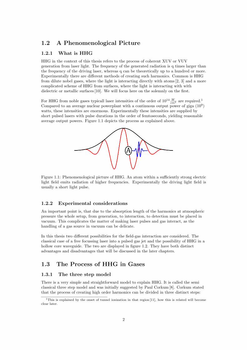
Compared to an average nuclear powerplant with a continuous output power of giga (109)watts, these intensities are enormous. Experimentally these intensities are supplied byshort pulsed lasers with pulse durations in the order of femtoseconds, yielding reasonableaverage output powers. Figure 1.1 depicts the process as explained above.

Figure 1.1: Phenomenological picture of HHG. An atom within a sufficiently strong electriclight field emits radiation of higher frequencies. Experimentally the driving light field isusually a short light pulse.

1.2.2 Experimental considerations

An important point is, that due to the absorption length of the harmonics at atmosphericpressure the whole setup, from generation, to interaction, to detection must be placed invacuum. This complicates the matter of making laser pulses and gas interact, as thehandling of a gas source in vacuum can be delicate.

In this thesis two different possibilities for the field-gas interaction are considered. Theclassical case of a free focussing laser into a pulsed gas jet and the possibility of HHG in ahollow core waveguide. The two are displayed in figure 1.2. They have both distinctadvantages and disadvantages that will be discussed in the later chapters.

1.3 The Process of HHG in Gases

1.3.1 The three step model

There is a very simple and straightforward model to explain HHG. It is called the semiclassical three step model and was initially suggested by Paul Corkum [8]. Corkum statedthat the process of creating high order harmonics can be divided in three distinct steps:

1This is explained by the onset of tunnel ionization in that region [11], how this is related will becomeclear later.

2

Figure 1.2: On the left HHG in a free focusing geometry, the gas is supplied via a pulsedgas jet. To the right HHG in a hollow core waveguide, the gas is distributed inside thewaveguide.

1. The initially bound electron appears with zero velocity in the light field.2. The electron is accelerated by the light field.3. Re-colliding with the atom it is strongly decelerated, emitting radiation.

The first step is here the most complicated one to explain in an understandable manner. Itwould be necessary to consider the electron in a quantum mechanical manner anddistinguish between several regimes depending on how strong the field is compared to theatomic potential. It is sufficient to know at this point that the electron can appear atseveral different times with respect to the external light field. This is due to inonizationprocess being probabilistic in nature.

Once it is subjected to the external field, the motion of the electron is defined by the forcesacting on it due to the light field.

Under certain circumstances the electron will then re-collide with the atom being almostinstantaneously decelerated to zero velocity, therefore emitting its kinetical energy plus thebinding energy in the form of electromagnetic radiation. An immediate deduction wouldbe that the maximal photon energy can not exceed the electron energy at impact plus theionization potential, due to the conservation of energy. Based on the three step model,very simple calculations reproducing characteristic features of HHG are possible.

1.3.2 Simulations based on the three step model

Figure 1.3 depicts simulations of the concept described above, assuming a cosine shapedlinearly polarized electric field. The different black lines represent one dimensionaltrajectories of electrons that have appeared at different times in the electric field with theproperties y(t0) = 0, meaning that the atoms appear directly at the position of the atomand v(t0) = 0, meaning that they have no initial velocity. Some of those electrons re-collidewith the atom, in other words they come back to y = 0, while others wiggle away from theatom.Above we deduced, that the maximal photon energy can not exceed the kinetic energy atimpact plus the ionization potential. Plotting the kinetic energy of the simulated electronsat the re-impact on the atom (see figure 1.4), we find that our model predicts that

Ephoton−max ≤ 3.17Up + Ip (1.1)

Where Up is the ponderomotive potential, that is in this case just a convenient way tocollect factors like the electron charge, the electron mass, the light frequency etc. and Ip

3

Figure 1.3: Different one-dimensional trajectories (black lines) for electrons appearing atdifferent times in the external field (red line).

being the ionization potential.2 This result agrees surprisingly well, with what has beenmeasured in experiments (see for example figure 2.7). There is also only a small deviationfrom expressions obtained in more sophisticated models [15].

Figure 1.4: Kinetic energy at the re-impact on the atom for different electron emission times.The emission time is given in terms of multiples of π, representing the phase of the drivingelectric field E ∝ cos(t).

1.3.3 Shortcomings of the presented picture

In the way it was presented here the three step model does not include any informationabout either the process of the transformation of kinetical energy to electromagneticradiation or about the phase of the generated light. This is due to the way it was narratedand not at all a shortcoming of the model. In the next chapter a fully quantum mechanicalpicture will be presented that includes all these informations and recreates the three stepmodel as a special case. Therefore for all remaining questions the reader should be referredto the next chapter.

2However it can be shown in a straightforward manner that Up represents the average kintetic energy ofa free electron in a monochromatic light field.

4

1.4 Introduction to Nonlinear Optics

In order to explain HHG in a more general way and to ultimatively answer the questionsat the end of the previous section the concept of nonlinear optics will be required.

1.4.1 Waves and harmonics

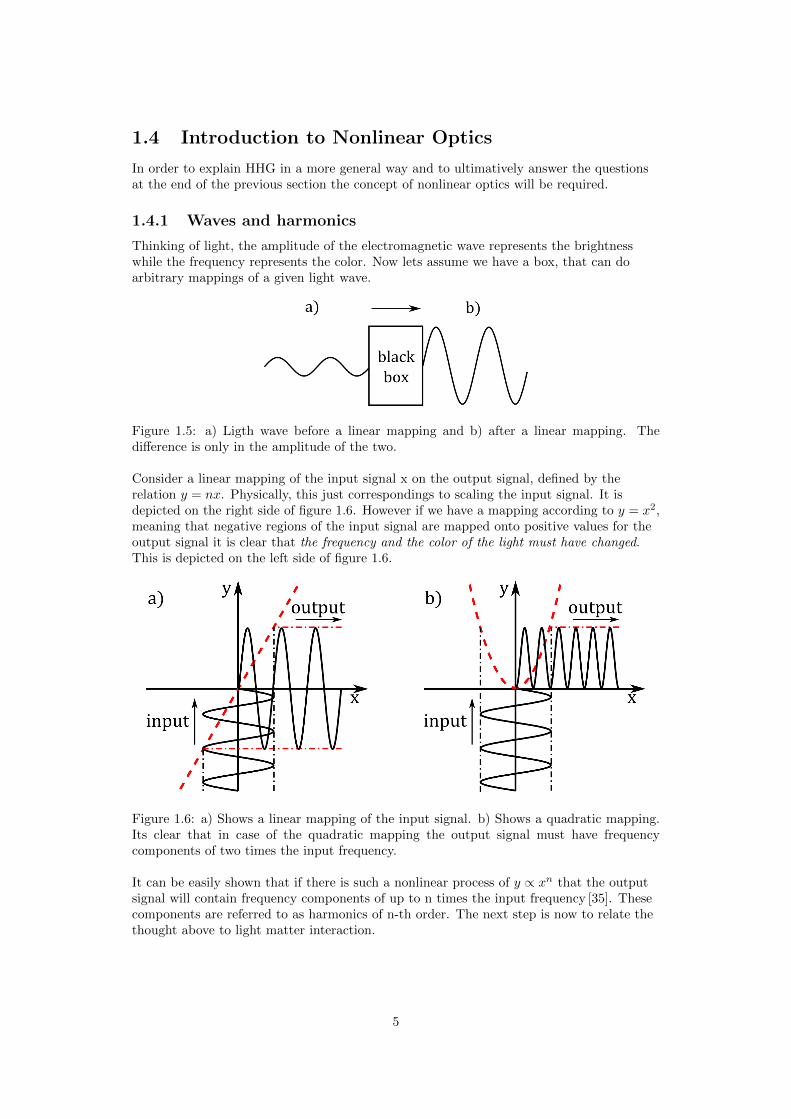
Thinking of light, the amplitude of the electromagnetic wave represents the brightnesswhile the frequency represents the color. Now lets assume we have a box, that can doarbitrary mappings of a given light wave.

Figure 1.5: a) Ligth wave before a linear mapping and b) after a linear mapping. Thedifference is only in the amplitude of the two.

Consider a linear mapping of the input signal x on the output signal, defined by therelation y = nx. Physically, this just correspondings to scaling the input signal. It isdepicted on the right side of figure 1.6. However if we have a mapping according to y = x2,meaning that negative regions of the input signal are mapped onto positive values for theoutput signal it is clear that the frequency and the color of the light must have changed.This is depicted on the left side of figure 1.6.

Figure 1.6: a) Shows a linear mapping of the input signal. b) Shows a quadratic mapping.Its clear that in case of the quadratic mapping the output signal must have frequencycomponents of two times the input frequency.

It can be easily shown that if there is such a nonlinear process of y ∝ xn that the outputsignal will contain frequency components of up to n times the input frequency [35]. Thesecomponents are referred to as harmonics of n-th order. The next step is now to relate thethought above to light matter interaction.

5

1.4.2 The transition from linear to nonlinear optics

Thinking of an atom-electron system in terms of classical physics, the electron will sit in aminimum of the potential V . This minimum is an equilibrium position in the sense, thatthe electron will always return to it, if only perturbed slightly.

Figure 1.7: An example for an equivalent one-dimensional potential for attractive inverse-square law forces as expected when thinking about electron and atom in a classical way,the potential is then given by V = a 1

x2 − b 1x [25]. The electron sits in a minimum of the

potential, being in an equilibrium position.

It will stay there as long as it has not enough energy to climb up the potential barrier,keeping it trapped. Taylor expanding the potential for the equilibrium position x0 the firstorder term will vanish due to the nature of the minimum.

V = V0 +1

2

∂2

∂x2V (x)

∣∣∣∣x0

(x− x0)2 +1

6

∂3

∂x3V (x)

∣∣∣∣x0

(x− x0)3 + . . . (1.2)

Recalling from our very basic physics lectures that the force is given by minus the gradientof V we find that closely around our equilibrium position the force is linear with thedisplacement:

F = − ∂2

∂x2V (x)

∣∣∣∣x0

(x− x0) (1.3)

If we now consider putting the electron further and further away from x0, the higher termsin the expansion will start to become important and expression 1.3 will gradually becomeinaccurate. In order to discuss the interaction of light with such a system, it is nownecessary to introduce the concept of the polarization P .

The polarization is a quantity related to the electric dipole moment, which is nothing elsebut a measure of the separation of positive and negative electrical charges in a system ofcharges. A very simple definition for an one electron system would be P = e(x− x0).Meaning that the polarization is just the charge e times its deviation from the equilibriumposition x0. Recalling that an electric field E exerts per definition a force on a charge, it isintuitive that this quantity must describe how light, being an electric field, interacts withatoms, being a system of charges. The force on an electron due to the presence of anelectric field with field strength E is given by:

F = eE (1.4)

The relation between the force and the field is linear and from above we know that therelation between the force and the electron displacement is also linear. This implies thatthe polarization must go linearly with the strength of the electric field. Writing this as anequation:

P = ε0χE (1.5)

6

Where ε0χ is just the proportionality constant. However, this is only valid in the vicintiyof the equilibrium position, as otherwise the higher terms in the Taylor expansion must beincluded, adding higher order terms of E in equation 1.5. The final question that needs tobe answered is, under which circumstances stays the electron closely to x0? A very simpleanswer is, as long as the electric field of the light is very much smaller than the electricfield of the atom at the equilibrium position. It turns out that the typical intensitiesneeded to observe these effects on noble gas atoms are rarely achieved, that is why it isusually sufficient to work in the framework of linear optics. Linear refers here to therelation between electric field and polarization.

1.4.3 Nonlinear optics

It was discussed what happens if the electric field is small compared to the atomic field,however this thesis deals with exactly the opposite case. What happens if the electric fieldis comparable to the atomic fields. From what was said so far we would expect to see thatthe polarization is proportional to higher orders of E and that therefore the polarizationwill contain harmonic frequency components up to the highest order of E.

In order to realize what that means for the interacting light propagation, the basic physicslectures have to be recalled, where it was told that the generation of electromagnetic fieldsis related to a temporal change in the dipole moment. This was typically illustrated on theexample of a simple antenna. In the introduction of the polarization it was said, that thepolarization is a measure for the atomic dipole moment. Therefore, imagining the boundelectrons around an atoms as tiny antennas, we expect not only harmonic frequencycomponents in the polarization but also in the driving laser field. A formal introduction tothe nonlinear polarization will follow in chapter 3.

1.5 Light Propagation in Waveguides

A waveguide is basically a structure that allows to contain a traveling wave. There is nolimitation to light or electromagnetic waves in general, also acoustic waveguides exist. Themost common waveguides are most probably the coaxial cable used for radio frequencytransmission and the glass fiber used for transmission of light signals.Contain does notneccesarily mean that the light waves can not escape, as we will see in later chapters.Waveguides can also be lossy. It is more certain properties of the wave propagation insidethe structure that defines a waveguide, what is meant by that will be more clear after thissection.

In general, the behavior of light can be described at different levels of complexity, startingfrom ray or geometrical optics, to wave optics, to electromagnetic optics and finallyquantum optics. These concepts became necessary for ever more detailed experimentalobservations. Some problems require the application of quantum optics while a large classof problems can be solved exactly in geometrical optics entirely without the otherconcepts. Propagation of light waves in waveguides can only be described in a satisfyingmanner dealing with electromagnetic optics, which is often very mathematical andinaccessible. However some properties of simple waveguides can be deduced in a ratherintuitive way using a combination of geometrical and wave optics.

1.5.1 Properties of simple waveguides

The requirement for a waveguide was stated as containing a traveling wave. It can beinterpreted as the condition, that the wave should reproduce itself inside the waveguide.The simplest geometry that could fulfill these requirements are two parallel perfect mirrors,

7

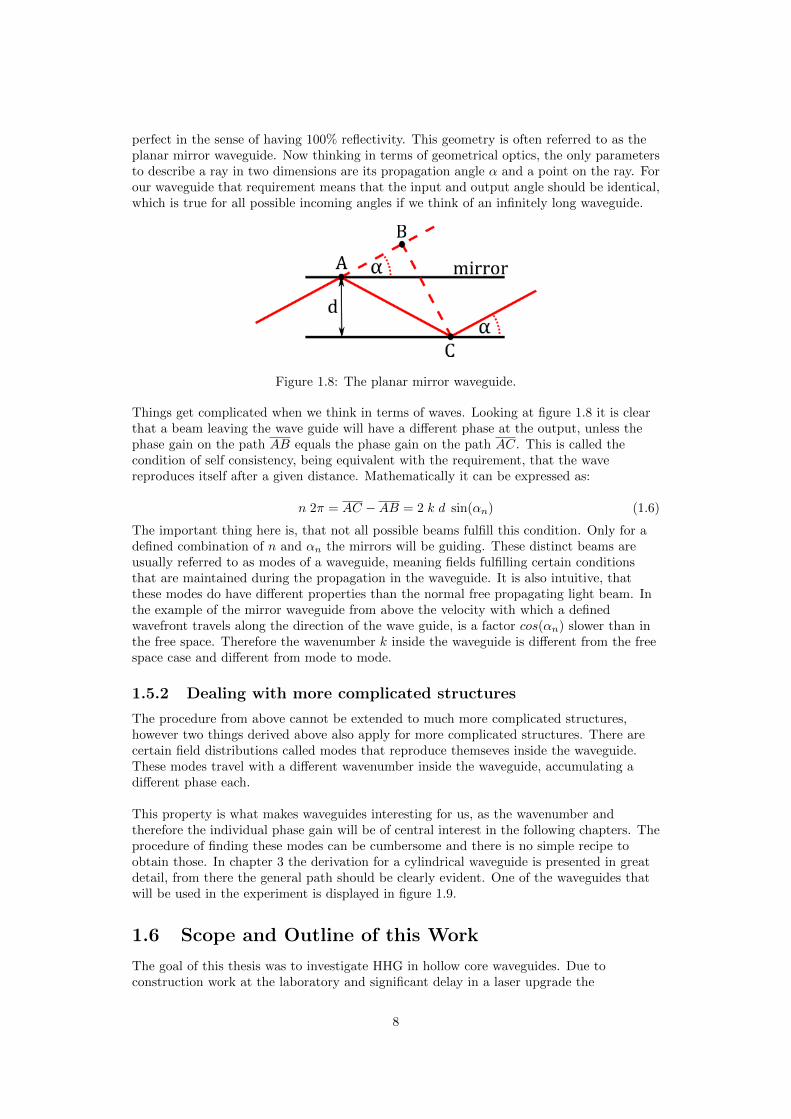
perfect in the sense of having 100% reflectivity. This geometry is often referred to as theplanar mirror waveguide. Now thinking in terms of geometrical optics, the only parametersto describe a ray in two dimensions are its propagation angle α and a point on the ray. Forour waveguide that requirement means that the input and output angle should be identical,which is true for all possible incoming angles if we think of an infinitely long waveguide.

Figure 1.8: The planar mirror waveguide.

Things get complicated when we think in terms of waves. Looking at figure 1.8 it is clearthat a beam leaving the wave guide will have a different phase at the output, unless thephase gain on the path AB equals the phase gain on the path AC. This is called thecondition of self consistency, being equivalent with the requirement, that the wavereproduces itself after a given distance. Mathematically it can be expressed as:

n 2π = AC −AB = 2 k d sin(αn) (1.6)

The important thing here is, that not all possible beams fulfill this condition. Only for adefined combination of n and αn the mirrors will be guiding. These distinct beams areusually referred to as modes of a waveguide, meaning fields fulfilling certain conditionsthat are maintained during the propagation in the waveguide. It is also intuitive, thatthese modes do have different properties than the normal free propagating light beam. Inthe example of the mirror waveguide from above the velocity with which a definedwavefront travels along the direction of the wave guide, is a factor cos(αn) slower than inthe free space. Therefore the wavenumber k inside the waveguide is different from the freespace case and different from mode to mode.

1.5.2 Dealing with more complicated structures

The procedure from above cannot be extended to much more complicated structures,however two things derived above also apply for more complicated structures. There arecertain field distributions called modes that reproduce themseves inside the waveguide.These modes travel with a different wavenumber inside the waveguide, accumulating adifferent phase each.

This property is what makes waveguides interesting for us, as the wavenumber andtherefore the individual phase gain will be of central interest in the following chapters. Theprocedure of finding these modes can be cumbersome and there is no simple recipe toobtain those. In chapter 3 the derivation for a cylindrical waveguide is presented in greatdetail, from there the general path should be clearly evident. One of the waveguides thatwill be used in the experiment is displayed in figure 1.9.

1.6 Scope and Outline of this Work

The goal of this thesis was to investigate HHG in hollow core waveguides. Due toconstruction work at the laboratory and significant delay in a laser upgrade the

8

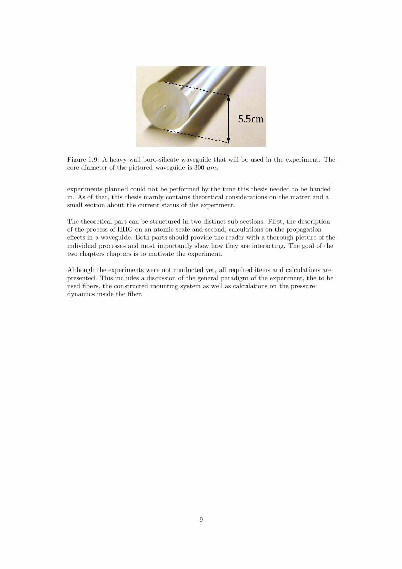
Figure 1.9: A heavy wall boro-silicate waveguide that will be used in the experiment. Thecore diameter of the pictured waveguide is 300 µm.

experiments planned could not be performed by the time this thesis needed to be handedin. As of that, this thesis mainly contains theoretical considerations on the matter and asmall section about the current status of the experiment.

The theoretical part can be structured in two distinct sub sections. First, the descriptionof the process of HHG on an atomic scale and second, calculations on the propagationeffects in a waveguide. Both parts should provide the reader with a thorough picture of theindividual processes and most importantly show how they are interacting. The goal of thetwo chapters chapters is to motivate the experiment.

Although the experiments were not conducted yet, all required items and calculations arepresented. This includes a discussion of the general paradigm of the experiment, the to beused fibers, the constructed mounting system as well as calculations on the pressuredynamics inside the fiber.

9

Chapter 2

Single-Atom Response

2.1 Introduction to the Atomic Polarization

In the previous chapter it has been stated on a qualitative level how high harmonicgeneration is explained within the three step model. Anyhow the narration was chosensuch that it is intuitive and simple. For instance, instead of saying the incidentelectromagnetic field distorts the Coulomb potential of the atom, thereby allowing parts ofthe electron wave function to reach the continuum through multi photon-, tunnel- or abovethreshold ionization. It was said an electron appears in the continuum. The followingpages should now introduce the conceptual context and derive a model on a fully quantummechanical basis. It can then be shown that in a special case this model reduces to thethree step model.The starting point here is something that has been hinted at already in the introduction,namely that the polarization ~P(ω) can be identified as a source term in the calculation ofelectric field propagation1. Therefore what needs to be found is a quantum mechanicaldescription of the polarization of the single atom. It is convenient to start with the verysimple model of an electron in a neutral atom. The polarization is then just given by

~P (t) = e~x(t) (2.1)

Where ~x(t) is the displacement from the equilibrium position. Quantum mechanically ~x(t)is given by the expectation value of the x operator, or in Dirac notation

x(t) = 〈Ψ, t|x |Ψ, t〉 (2.2)

This basically only leaves us with the task of calculating |Ψ, t〉, or more explicitly findingthe solutions of the Schrodinger equation for the given Hamiltonian of the system.

−ih ∂∂t|Ψ, t〉 = H |Ψ, t〉 (2.3)

The interaction Hamiltonian is here H = H0 + Vlight(x, t), where H0 denotes theHamiltonian without the electromagnetic field. Solving the time dependent Schrodingerequation (eq. 2.3) (TDSE) exactly is a very tedious undertaking as for a real atom with afew electrons H0 can be almost arbitrarily complicated. Therefore, as of today, exactsolutions are only available in a very limited range of cases. Anyhow, there will be a shortside note on these numerical TDSE calculations later in this text. What this chapter willfocus on is a very intuitive set of approximations to the TDSE that allows us to properlyexplain the behavior of HHG in a reasonable region of experimental parameters.

1see chapter 3 for a more thorough discussion

10

2.2 Modeling the Electron Wave function

2.2.1 The single active electron approximation

As stated in the previous section, the first major source for complications is H0 as itinvolves interaction terms among individual electrons. These interaction terms not onlybreak the spherical symmetry but also couple the individual wave functions of theelectrons. Equation 2.4 represents such a multi particle Hamiltonian for an i-electronsystem.

H0 =∑i

p2i

2mi+ Vnuc(ri) +

∑i 6=j

Vi−j(rij)

(2.4)

In that expression the first term in the sum is just the kinetic energy of the i-th electron,the second term is the potential energy of the i-th electron due to the positive charges inthe nucleus and the last term represents the interaction potential between the i-th and thej-th electron. There are now several strategies to circumvent the problems stated abovewhile still maintaining a high degree of generality, notably the central fieldapproximation [1]. Anyhow for simplicity we will choose none of these and go for the singleactive electron approximation. The complete Hamiltonian becomes then

H =p2

2m+ Veff (r) + Vlight(x, t). (2.5)

In this case the effective core potential Veff (r) is chosen such that for the given atom theright ionization potential Ip is obtained. Vlight denotes the potential exerted by theexternal light field that is needed for the following discussion.

2.2.2 Introduction of essential states

Now even with a single particle Hamiltonian the problem can still be quite complicated.For instance for the case of the single electron in a spherical symmetric potential theSchrodinger equation constitutes a Laplace equation, best written in spherical polarcoordinates.

−ih ∂∂t

Ψ(r,Θ,Φ, t) = − h2

2m∆Ψ(r,Θ,Φ, t) + V (r)Ψ(r,Θ,Φ, t)

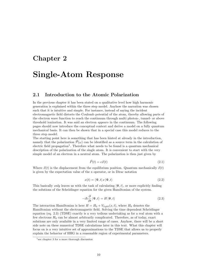
With the well known result that there is an infinite set of linearly independent solutionsΨ(r,Θ,Φ, t)n,l to this equation. The actual function describing the system may then be alinear superposition of these. Therefore the time evolution of the system is given by theindividual time evolution of the infinitely many solutions. The concept becomes muchmore familiar if we refer to the individual solutions as individual states. In practice itsoften sufficient to consider only a few involved states. A good example for this is the twostate formalism regularly used in laser theory or quantum information. There the totalwave function is assumed to be of the shape |Ψ〉 = a |1〉+ b |2〉. Here a similar approachwill be applied. It will be assumed that the electron is in its ground state |0〉 before thelight is interacting with the atom. Further it couples from there directly into a continuumof momentum eigenstates |b, p〉 without occupying any non virtual intermediate states onthe way there. Figure 2.1 depicts the choice of essential states.Therefore the wave function is given in first order perturbation theory by

|Ψ, t〉 = exp

(iIpt

h

)[a(t) |0〉+

∫b(p, t) |p〉 dp3

](2.6)

Where Ip denotes the ionization potential or the Eigen energy of |0〉. We have implicitlyassumed, that the zero in energy is at the groundstate energy. A further simplification can

11

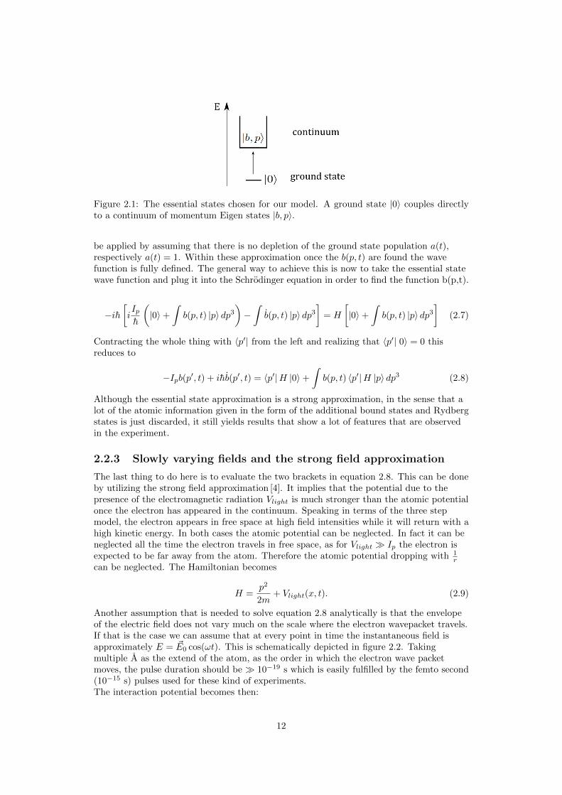
Figure 2.1: The essential states chosen for our model. A ground state |0〉 couples directlyto a continuum of momentum Eigen states |b, p〉.

be applied by assuming that there is no depletion of the ground state population a(t),respectively a(t) = 1. Within these approximation once the b(p, t) are found the wavefunction is fully defined. The general way to achieve this is now to take the essential statewave function and plug it into the Schrodinger equation in order to find the function b(p,t).

−ih[iIph

(|0〉+

∫b(p, t) |p〉 dp3

)−∫b(p, t) |p〉 dp3

]= H

[|0〉+

∫b(p, t) |p〉 dp3

](2.7)

Contracting the whole thing with 〈p′| from the left and realizing that 〈p′| 0〉 = 0 thisreduces to

−Ipb(p′, t) + ihb(p′, t) = 〈p′|H |0〉+

∫b(p, t) 〈p′|H |p〉 dp3 (2.8)

Although the essential state approximation is a strong approximation, in the sense that alot of the atomic information given in the form of the additional bound states and Rydbergstates is just discarded, it still yields results that show a lot of features that are observedin the experiment.

2.2.3 Slowly varying fields and the strong field approximation

The last thing to do here is to evaluate the two brackets in equation 2.8. This can be doneby utilizing the strong field approximation [4]. It implies that the potential due to thepresence of the electromagnetic radiation Vlight is much stronger than the atomic potentialonce the electron has appeared in the continuum. Speaking in terms of the three stepmodel, the electron appears in free space at high field intensities while it will return with ahigh kinetic energy. In both cases the atomic potential can be neglected. In fact it can beneglected all the time the electron travels in free space, as for Vlight � Ip the electron isexpected to be far away from the atom. Therefore the atomic potential dropping with 1

rcan be neglected. The Hamiltonian becomes

H =p2

2m+ Vlight(x, t). (2.9)

Another assumption that is needed to solve equation 2.8 analytically is that the envelopeof the electric field does not vary much on the scale where the electron wavepacket travels.If that is the case we can assume that at every point in time the instantaneous field isapproximately E = ~E0 cos(ωt). This is schematically depicted in figure 2.2. Takingmultiple A as the extend of the atom, as the order in which the electron wave packetmoves, the pulse duration should be � 10−19 s which is easily fulfilled by the femto second(10−15 s) pulses used for these kind of experiments.The interaction potential becomes then:

12

Figure 2.2: The figure shows the electric field of two pulses compared to the extend of thepropagation of the electron wavefunction around an atom A. In a) the envelope functionchanges significantly on the scale of the path of the wave function, whereas in b) the changeis way smaller. For long enough pulses the envelope function can be assumed as beingconstant.

Vlight(x, t) = −xeE0 cos(ωt) (2.10)

Therefore the final Hamiltonian has the form:

H =p2

2m− xeE0 cos(ωt). (2.11)

It has the very nice property that the momentum eigenstates are obviously eigenstates ofthe first part, while the second one leads to the well known and discussed dipole matrixelement once plugged into equation 2.8.

−Ipb(p′, t) + ihb(p′, t) = −eE0 cos(ωt) 〈p′|x |0〉+ (2.12)

p′2

2mb(p′, t)− eE0 cos(ωt)

∫b(p, t) 〈p′|x |p〉 dp3

Using 〈p′|x |p〉 = ih ∂∂pδpp′ allows us to write for b(p, t):

b(p, t) = −i 1h

(p2

2m+ Ip

)b(p, t)− eE0 cos(ωt)

∂

∂pb(p, t) +

ieE0

hcos(ωt) 〈p|x |0〉 (2.13)

This equation can be rewritten in a relativistic form by substituting the canonicalmomentum ~Π for the relativistic free electron in an external electromagnetic field [29] forthe kinematic momentum used before.2

~p ≡ ~Π = ~p+ e ~A (2.14)

Where p is, as before, the kinematic momentum and A is the vector potential. Equation2.13 can then be cast into a closed form [4]:

b(p, t) = i

∫ t

0

eE0

hcos(ωt′)dx

(p+ e ~A(t)− e ~A(t′)

)× (2.15)

exp

(−i∫ t

t′

1

h

[1

2m

(p+ e ~A(t)− e ~A(t′′)

)2

+ IP

]dt′′)dt′

2The expression in Jackson [29] is in Gaussian units, here SI units are used.

13

The general path for doing the transition from equation 2.13 to 2.16 is to substitute ∂b∂p by

∂b∂t

∂t∂p . Equation 2.16 can also be written in terms of the canonical momentum:

b(p, t) = i

∫ t

0

eE0

hcos(ωt′)dx

(Π− e ~A(t′)

)× (2.16)

exp

(−i∫ t

t′

1

h

[1

2m

(Π− e ~A(t′′)

)2

+ IP

]dt′′)dt′

dx(p) denotes here the dipole matrix element 〈p|x |0〉. With the vector potential for our

linearly polarized laser field being defined as ~E = − ∂∂t~A:

~A =

(−E0

ωsin(ωt), 0, 0

)(2.17)

Therefore b(p, t) can be calculated from experimentally available parameters and thus thewave function can be estimated. Equation 2.17 can also be written in a more compact wayby introducing:

S(Π, t, t′) =

∫ t

t′

1

h

[1

2m

(Π− e ~A(t′′)

)2

+ IP

]dt′′ (2.18)

The inner part of the integral can be identified as a Lagrangian of the free electron in aconstant potential −IP , which makes the whole integral the quasi classical action of thefree electron propagation. If this analogy holds we would expect from a classical point ofview that the extremal values of the action provide us with the actual motion of theelectron. Anyhow this will be discussed at a later point in more detail. The to beevaluated expression for b(p,t) is at last:

b(p, t) = i

∫ t

0

eE0

hcos(ωt′)dx

(Π− e ~A(t′)

)exp (−iS(Π, t, t′))dt′ (2.19)

2.3 Discussion of the Dipole Matrix Element

Having obtained a proper wave function, the next step is to substitute it in the definitionof the dipole matrix element (given in equation 2.2).

x(t) =

[〈0|+

∫b∗ 〈p| dp3

]x

[|0〉+

∫b |p′〉 dp′3

](2.20)

This results in four separate matrix elements:

x(t) = 〈0|x |0〉+

∫b(t) 〈0|x |p′〉 dp′3 +

∫b∗(t) 〈p|x |0〉 dp3 +

∫ ∫|b(t)|2 〈p|x |p′〉dp′3dp3

(2.21)The first term describes the coupling from the ground state to the ground state. Thinkingof x in terms of creation and annihilation operators this term should vanish. Term numbertwo and three are terms representing ground state-continuum coupling and the last termdescribes continuum-continuum coupling.

x(t) = x0−p(t) + xp−0(t) + xc−c(t) (2.22)

14

2.3.1 Continuum-continuum coupling

Upon generalizing the essential state model with regard to the parity of the continuumstates, it can be shown that the dipole matrix element for continuum-continuum couplingmust be null for all t. The generalization allows now, instead of one continuum withundefined properties, two continua |b, p〉 and |c, p〉 with different parity. This is convenientdue to the dipole operator x being odd. Therefore all allowed transitions must involve both|b, p〉 and |c, p〉. Figure 2.3 depicts this model.

Figure 2.3: The essential states chosen for this argument. A groundstate |a〉 with a givenparity and two continua |b, p〉 and |c, p〉 with different parity.

In this derivation, as only the qualitative result is sufficient, it will be assumed thate = h = c = 1. Other than that, the rest of the derivation works in the same manner as in2.2.2. The essential state wave function becomes:

|Ψ, t〉 = exp(iI0ht)

[a(t) |a〉+

∫b(p, t) |b, p〉 dp3 +

∫c(p, t) |c, p〉 dp3

](2.23)

Introducing an interaction potential Vi(t) = V0f(t), with the restriction that it couples |a〉only to |c〉 the following three equations can be obtained by substituting equation 2.23 intothe Schrodinger equation [12].

a = − iV0(t)

2

∫c(p, t)dp (2.24)

b = −ib(p, t)− iF (t)

∫d(p, p′)c(p, t)dp′

c = −ic(p, t)− iV0(t)

2a(t)− iF (t)

∫d(p, p′)b(p, t)dp′

Where F(t) is the field coupling the two continuum states and d(p, p′) is the correspondingdipole matrix element. Under the assumption that the dipole matrix element is asymmetric function d(p, p′) = d(p′, p) and using the wave function above in the definitionof x(t) given in equation 2.2, an expression for the continuum continuum contribution canbe found.

xc−c(t) =

∫ +∞

−∞

∫ +∞

−∞d(p, p′) [b(p, t)c∗(p′, t) + b∗(p, t)c(p′, t)] dpdp′ (2.25)

It can be shown that xc−c(t) is zero for all t. Anyhow the argument is tricky. It can beshown [12] that if the initial values of a(t), b(p, t) and c(p, t) fulfill certain symmetryconditions these symmetries are conserved in time. Explicitly if a(t) = a∗(t),b(−p, t) = −b∗(p, t) and c(−p, 0) = c∗(p, t) is fulfilled for t = 0 it will be fulfilled also at alllater times.3 The conditions, although initially looking complicated, are fulfilled by

3It can easily be shown for a(t) by writing a(t) and a∗(t) in its explicit form, anyhow for the other twoparameters its a bit more complicated.

15

a(0) = 1, b(p, 0) = c(p, 0) = 0 which are the usual starting parameters. Splitting the

integrals∫ +∞−∞ dp in equation 2.25 into

∫ 0

−∞ dp+∫ +∞

0dp and inserting the symmetries we

find xc−c(t) = 0.

2.3.2 A physical interpretation

The results of the previous section lead us to the conclusion that also in the calculation ofthe expectation value of x(t) the c− c terms can in general be neglected. Equation 2.22becomes then

x(t) = x0−p(t) + x∗p−0(t) (2.26)

Or more conveniently

x(t) =

∫[b(t) d∗x(p, t) + c.c.] dp3. (2.27)

Having the expression 2.27 for x(t) and having linked b(t) to experimentally availableparameters like the vector potential and the field strength, we can proceed to calculatingx(t) explicitly.

x(t) = i

∫ +∞

−∞

[∫ t

0

eE0

hcos(ωt′)dx

(Π− e ~A(t′)

)× (2.28)

d∗x

(Π− e ~A(t)

)exp (−iS(Π, t, t′))dt′ + c.c.

]dΠ3

The different terms can now be interpreted according to [4, 21]. The first term in the

integral eE0

h cos(ωt′)dx

(Π− e ~A(t′)

)is the part of an electron wave packet to make the

transition to the continuum at time t′ with canonical momentum Π. exp (−iS(Π, t, t′)) canbe identified as the free space propagator, governing the phase gain of that part of the

wave packet during propagation. Finally d∗x

(Π− e ~A(t)

)describes the recombination at

time t. This resembles the semi classical three step model described earlier anyhow withthe distinction that we are considering and calculating all possible pathways for theelectron wave packet. The possible interferences between these quantum pathsdistinguishes the two models, as for the semi classical case only whole electrons arepropagated. The formulation here, talking of quantum paths and obtaining the final resultby considering all possible pathways and weighting them acordingly, points very much inthe direction of a Feynman path integral approach. Although not done here its worthpointing out that the problem can be fully treated in the path integral framework [22].

2.4 Estimating the Dipole Strength

In order to relate these considerations to possible experiments, it would be beneficial tofurther break down the expression obtained for the atomic dipole moment (eq. 2.29).

2.4.1 The saddle point approximation in 1-D

Switching the order of integration in equation 2.29, the integration in Π can be consideredfirst. In doing so, the different terms are evaluated in how fast they change with respect tothe canonical momentum Π. According to Lewenstein [4] the variation of the dipolemoments in Π are much smaller than the variation of the quasi classical action. This leavesus with an equation of the type:

16

A =

∫ +∞

−∞f(~x)eig(~x)d3x (2.29)

In order to explain the mathematical method used for evaluating these kinds of equationsits educative to consider the one dimensional case first, where

A1D =

∫ +∞

−∞f(x)eig(x)dx (2.30)

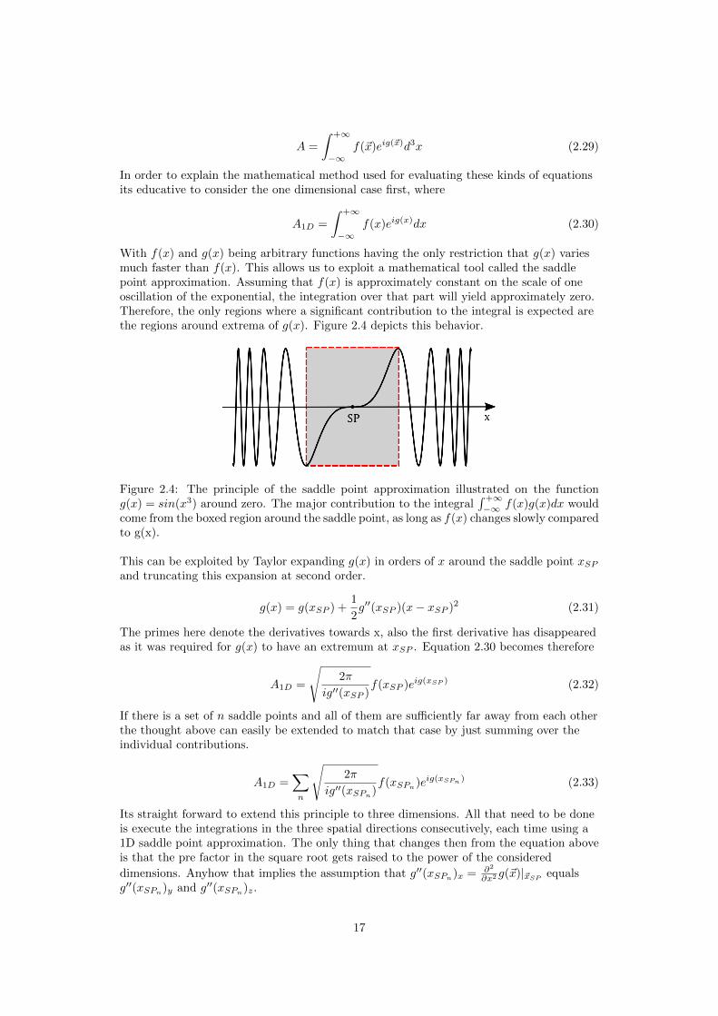
With f(x) and g(x) being arbitrary functions having the only restriction that g(x) variesmuch faster than f(x). This allows us to exploit a mathematical tool called the saddlepoint approximation. Assuming that f(x) is approximately constant on the scale of oneoscillation of the exponential, the integration over that part will yield approximately zero.Therefore, the only regions where a significant contribution to the integral is expected arethe regions around extrema of g(x). Figure 2.4 depicts this behavior.

Figure 2.4: The principle of the saddle point approximation illustrated on the functiong(x) = sin(x3) around zero. The major contribution to the integral

∫ +∞−∞ f(x)g(x)dx would

come from the boxed region around the saddle point, as long as f(x) changes slowly comparedto g(x).

This can be exploited by Taylor expanding g(x) in orders of x around the saddle point xSPand truncating this expansion at second order.

g(x) = g(xSP ) +1

2g′′(xSP )(x− xSP )2 (2.31)

The primes here denote the derivatives towards x, also the first derivative has disappearedas it was required for g(x) to have an extremum at xSP . Equation 2.30 becomes therefore

A1D =

√2π

ig′′(xSP )f(xSP )eig(xSP ) (2.32)

If there is a set of n saddle points and all of them are sufficiently far away from each otherthe thought above can easily be extended to match that case by just summing over theindividual contributions.

A1D =∑n

√2π

ig′′(xSPn)f(xSPn

)eig(xSPn ) (2.33)

Its straight forward to extend this principle to three dimensions. All that need to be doneis execute the integrations in the three spatial directions consecutively, each time using a1D saddle point approximation. The only thing that changes then from the equation aboveis that the pre factor in the square root gets raised to the power of the considered

dimensions. Anyhow that implies the assumption that g′′(xSPn)x = ∂2

∂x2 g(~x)|~xSPequals

g′′(xSPn)y and g′′(xSPn

)z.

17

A =∑n

(2π

ig′′(xSPn)

) 32

f(xSPn)eig(xSPn ) (2.34)

Applying this principle on x(t) its helpful to write it in a convenient form before.

x(t) = i

∫ t′

0

[∫ +∞

−∞f(Π, t, t′) exp (−iS(Π, t, t′)) dΠ3

]dt′ + c.c. (2.35)

Therefore analogously to equation 2.35

x(t) = i

∫ t′

0

[∑n

(2π

iS′′(ΠSPn, t, t′)

) 32

f(ΠSPn, t, t′) e−iS(ΠSPn ,t,t

′)

]dt′ + c.c. (2.36)

There are now two problems in interpreting expression 2.36. The first is how to find thesaddle point in the first place and the second is how to interpret S′′(ΠSPn , t, t

′). Anyhowlatter is easily addressed as:

S′′(ΠSPn , t, t′) =

[d2

dΠ2

∫ t

t′

1

h

[1

2m

(Π− e ~A(t′′)

)2

+ IP

]dt′′]

ΠSPn

(2.37)

=1

hm

∫ t

t′1dt′′ =

τ

hm

Additionally to that, t′ can be substituted by t′ = t− τ and therefore the integrationchanges from dt′ to −dτ . By doing so the integration boundaries can extended to cover0 ≤ τ <∞ circumventing causality issues.

x(t) = i

∫ ∞0

[∑n

(2πhm

ε+ iτ

) 32

f(ΠSPn , t, t′) exp (−iS (ΠSPn , t, τ))

]dτ + c.c. (2.38)

The additional ε term appearing in the saddle point prefactor is first of all a mathematicalnecessity to prevent the integral from diverging at τ = 0. [4] The whole prefactor has a nicephysical interpretation, being a factor accounting for quantum diffusion of the wave packetdeposited to the continuum. This means, that while the electron wave packet travels in thecontinuum it expands, therefore, the longer it travels the smaller will be the overlapintegral with the initial state wave function.

2.4.2 Saddle points of the quasi classical action

The saddle points of the quasi classical action are defined by the extrema of S(Π, t, t′) withrespect to Π:

∇Π S(ΠSPn, t, t′) = ∇Π

∫ t

t′

1

h

[1

2m

(Π− e ~A(t′′)

)2

+ IP

]dt′′ = 0 (2.39)

Further the nabla operator can be applied before the integral, as the initial canonicalmomentum Π is independent of t′′. Therefore:

0 =

∫ t

t′

1

m

(Π− e ~A(t′′)

)dt′′ (2.40)

The expression in the integral represents now the particle momentum divided by the massand corresponds to the particle velocity. Therefore the condition for the saddle point canbe broken down to

0 = [r]tt′ = r(t)− r(t′) (2.41)

18

Where r(t) denotes the location of the electron at time t. This has a very niceinterpretation, recalling from before that t′ has been identified as the electron emissiontime. The dominant contribution to the expectation value of x(t) comes from the electronsbeing ejected from the nucleus but then re encounter it while traveling in theelectromagnetic field. Again the semi classical picture appears to be correct.

Figure 2.5: A possible quantum path contributing to the expectation value x(t) of the dipoleoperator. a) At t − τ the part of the electron wave function is ejected into the continuumwith a canonical momentum ΠSP . b) The electron wave packet propagates for a time periodτ in the continuum. c) The wave packet comes back to its initial position at the time t.

Although the train of thought above did not directly add anything to the progress ofcalculating x(t), the next few lines will show how the the physical insight gained about thecharacter of t and t′ and the boundary conditions in r(t) and r(t− τ) can be used toestimate S(ΠSP−n, t, t

′). What we are looking for is the momentum with which theelectron is emitted into the continuum ΠSP−n. It can be obtained following a strictlyclassical consideration of the electron trajectory. Introducing the time of flight τ = t′ − twe can write:

pst(t) =

∫ t

t−τF (t)dt+ p0 (2.42)

In the beginning of these calculations (see 2.2.3) we assumed the electric field to be of theshape F (t) = eE0cos(ωt). It was shown above, that the boundary conditions at the saddlepoint are given by r(t− τ) = r(t) = 0. Therefore equation 2.42 has to be integratedanother time to obtain:

r(t) =

∫ t

t−τ

pst(t)

mdt =

[− eE0

mω2cos(ωt) + p0t+ r0

]tt−τ

(2.43)

Implementing the boundary conditions that yields

ΠSP ≈ p0 =eE0

mω2τ[cos(ωt)− cos(ω(t− τ))] (2.44)

Using the result above together with the explicit form of the vector potential given inequation 2.17 allows us to calculate the integral in the definition of the quasi classicalaction (eq. 2.18).

SSP (t, τ) =

∫ t

t−τ

1

h

[1

2m

(ΠSP − e ~A(t′′)

)2

+ IP

]dt′′ (2.45)

=1

h

[Ipτ + 2Up

∫ t

t−τ

(1

ωτ[cos (ωt)− cos (ω(t− τ))] + sin(ωt′′)

)2

dt′′

]

=1

h

[(Ip + Up)τ − 2

Upτω2

[1− cos(ωτ)]− UpωC(τ) cos (ω[2t− τ ])

]

19

Where the function C(τ) is defined as:

C(τ) = sin2(ωτ)− 4

τωsin2

(ωτ2

)(2.46)

Further it was made use of the ponderomotive potential Up =e2E2

0

4mω2 . It is at this positionimportant to point out that

Up ∝ E20 ∝ ILaser, (2.47)

as the laser intensity ILaser will lateron be the quantity of interest in the discussion of theporpagation effects.

2.4.3 Modeling the dipole matrix elements.

The findings in the previous two sections, together with equation 2.29 culminate inequation 2.49.

x(t) = i

∫ ∞0

[∑n

(2πhm

ε+ iτ

) 32 eE0

h cos (ω[t− τ ]) dx

(ΠSP−n(t, τ)− e ~A(t− τ)

)× (2.48)

d∗x

(ΠSP−n(t, τ)− e ~A(t)

)exp (−iSSP−n (t, τ))

]dτ + c.c.

It becomes clear at that point, that the only thing now missing is some model for thedipole matrix elements dx (Π) and d∗x (Π). The task itself is initially fairly straight forward.Pick a ground state wave function and calculate the overlap integral 〈Π|x |0〉 with the tobe investigated momentum eigenstate. This is then the end of the part where the taskpretends to be easy, as already the question of which ground state wave function to chooseand how the momentum states are considered is problematic. For instance describing theelectron momentum eigenstates in the presence of an electric field, becomes a conceptuallynontrivial undertaking, if done relativistically correct (see [23]). In reference [4] the twosimplest possible models are presented for a Gaussian ground state wave function and forHydrogen-like atoms with plain wave states instead of the apropriate Volkow states asmomentum eigenstates. Anyhow it would go beyond the scope of this thesis to present adeeper theoretical discussion on that matter. Quoting the solution for the Hydrogen-likeatom in the limit h = ω = m = 1 [4, 24]:

d(Π) ≈ i(

27/2(2Ip)5/4

π

)Π

(Π2 + (2Ip)2)3 (2.49)

For the further discussion its important to clarify that dipole strength refers to ‖(x(ω))‖2.Figure 2.6 shows simulations of the dipole strength as a function of the harmonic order.The results resemble the features of hhg data obtained experimentally on suitable systems,an example of this data is displayed in figure 2.7. In particular the typical plateau with acutoff at approximately 3.17Up + Ip [18] can be observed, this result is also what wasobtained in the introduction by completely classical calculations. A more detaileddiscussion of the model and the quality of the calculations will be omitted, as it would leadto far. For a thorough discussion the reader is referred to [22, 19, 18] and the referencestherein. It is sufficient for our purposes to have shown at this point, that the model wehave chosen shows a qualitatively correct behavior and that it agrees, respectively deviatesonly slightly, from the predictions of the semi classical model.

20

Figure 2.6: Simulation of the dipole strength |x(ω)| according to the model described in thissection in the limit of h = ω = m = e = ω = 1. The parameters are Up = 8, Ip = 5.

2.4.4 The dipole phase of individual harmonics

This section contains now the second major item the whole chapter was working towards.The information about how the microscopic phase of the individual harmonics behaveswith respect to the driving electromagnetic field. Although not immediately obvious thisinformation is crucial for calculating the harmonic buildup (see the following chapter). Inthe current model there are only two experimentally accessible quantities assuming thetype of atoms in consideration are fixed. The wavelength and the ponderomotive potential,whereas the latter is equivalent to the intensity of the driving field. Now focusing on theintensity dependence, the dipole strength and the atomic phase are calculated for differentvalues of Up. The term atomic phase is there referring to the argument of x(ω), itrepresents the phase gain in the whole process of emission, propagation and recombinationof the free electron.Picture 2.8 shows a typical result of these calculations. It is important to see that theatomic phase changes significantly compared to π even within small variations of theintensity, further the dependence of the atomic phase on the intensity seems to first orderlinear. This behavior is independent of the harmonic order. It seems apropriate toapproximate the atomic phase as

φatomic ∝ αUpIlight (2.50)

The question is how the atomic phase relates to the dipole phase, which is calculatedrelative to the incident electric field or more specifically to the generated harmonic atother points in space. Anyhow this discussion will be postponed until section 3.2.4.

2.5 Conclusion on Chapter 2

To briefly summarize the findings of this chapter: It was shown, that a very simpleessential state model is sufficient to explain the qualitative behavior of HHG. In variouspositions of the derivation analogies between the quasi classical picture and this fullyquantum mechanical picture can be found. This extends up to the point where theindividual terms in the quantum mechanical representation of the dipole operator can beidentified with the three steps suggested by Corkum.The introduction, or more correctly identification, of the quasi classical action allows us touse its properties to predict the possible electron paths in the electromagnetic field and

21

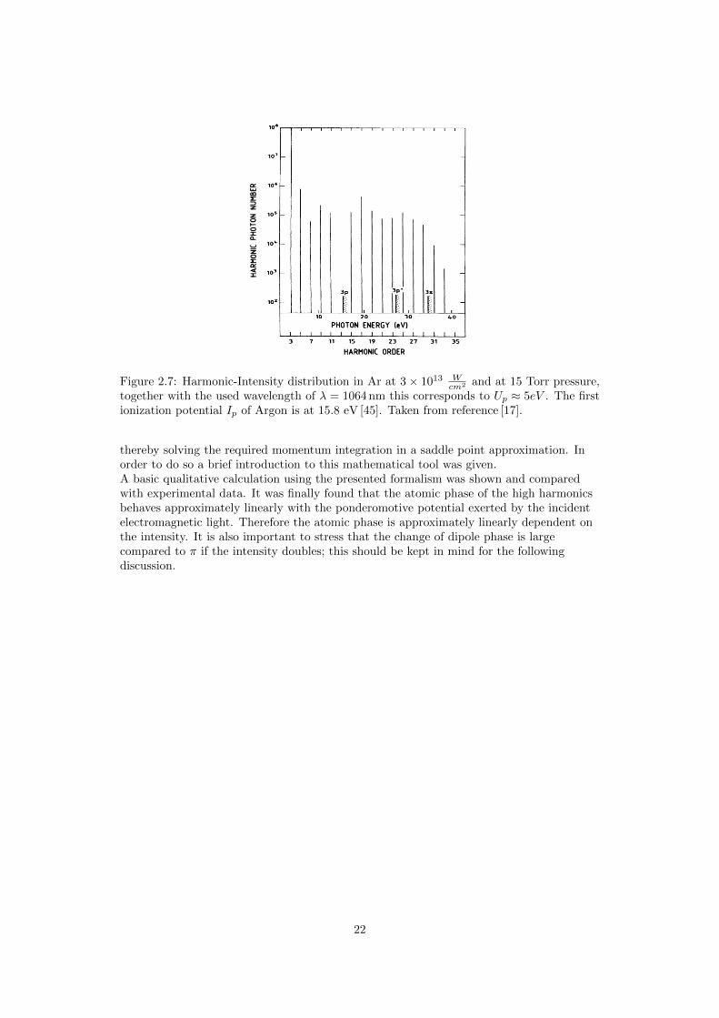
Figure 2.7: Harmonic-Intensity distribution in Ar at 3× 1013 Wcm2 and at 15 Torr pressure,

together with the used wavelength of λ = 1064 nm this corresponds to Up ≈ 5eV . The firstionization potential Ip of Argon is at 15.8 eV [45]. Taken from reference [17].

thereby solving the required momentum integration in a saddle point approximation. Inorder to do so a brief introduction to this mathematical tool was given.A basic qualitative calculation using the presented formalism was shown and comparedwith experimental data. It was finally found that the atomic phase of the high harmonicsbehaves approximately linearly with the ponderomotive potential exerted by the incidentelectromagnetic light. Therefore the atomic phase is approximately linearly dependent onthe intensity. It is also important to stress that the change of dipole phase is largecompared to π if the intensity doubles; this should be kept in mind for the followingdiscussion.

22

Figure 2.8: Dipole strength and atomic phase of the 35 harmonic as a function of Up. Theionization potential was chosen to Ip = 1.5 which corresponds approximately to the valuefor argon in the given units.

23

Chapter 3

Propagation Equations andPhase Matching in Waveguides

3.1 Introduction to Propagation Equations

3.1.1 The general problem

It has been shown in the previous chapter that the atomic response to the incidentradiation results in an intensity dependent phase and a dipole strength for a givenharmonic order. In the second step of the theoretical description we have to direct ourattention now towards the macroscopic propagation of the harmonic field. The crux of thebiscuit is here to find solutions to the Maxwell equations that accurately describe theevolution while not getting too complicated to solve. The starting point for this is here thevectorial Helmholtz equation in time domain which can be directly obtained from the freespace Maxwell equations (sketch of the derivation is given in 3.3.1).

∇2 ~E − 1

c2d2

dt2~E = µ0

d2

dt2~P (3.1)

The next step is to transform this equation into frequency domain and introduce the usualexpansion of ~P in orders of ~E . Cursive letters shall denote here Fourier transformedquantities.

∇2~E +ω2

c2~E = −µ0ω

2ε0

[χ(1)~E + (χ(2)~E)~E + (. . .)

](3.2)

Where the quantities χn represent the n-th order dielectric susceptibility tensor. It is nowuseful to write total electric field as sum of the individual harmonics.

~E(~r, ω) =∑q

~Eq(~r, ω) (3.3)

Combining the above with equation 3.2 a set of q differential equations is obtained. Thewhole set is coupled due to the higher order terms in ~E .

3.1.2 Linearization and the Born approximation

The complexity of solving the wave equations is drastically reduced by keeping theequation linear in ~E and assuming that the ~Eq are not overlapping in frequency domain.

Therefore we drop the terms of order greater than one in the power expansion of ~P andreintroduce the coupling indirectly with an additional nonlinear polarization dependingonly on the fundamental.

24

~Pq(~r, w) = ε0χ(1)q~Eq(~r, w) + ~PNLq (~EF ) (3.4)

~EF denotes there the electric field of the fundamental. This step might sound bold but hasproven to be very useful in the past [13, 14, 16]. The propagation is then described for theq-th harmonic and the fundamental by the following set of equations:

∇2~EF +ω2

c2n2F~EF = 0 (3.5)

∇2~Eq +ω2

c2n2q~Eq = − ω2

ε0c2~PNLq (~EF ) (3.6)

Where we have made use of the fact that the linear refractive index is defined asn2q = 1 + χ

(1)q . The fundamental is thus propagating just like in the case without harmonic

generation. Unconsciously we made an approximation that is usually referred to as theBorn approximation. It means that we are treating the Harmonics as a perturbation to theinitial field. Therefore to first order the fundamental remains unchanged. It is alsoimportant to note that with this approach no interaction effects between the harmonicsitself are included anyhow it can easily be extended to include for instance low orderharmonics.The general strategy to obtain a complete solution is then to compute first thepropagation of the fundamental through the geometry. And then in a second step use theresults to compute the propagation of the harmonic in question.

3.1.3 The free propagation case and the co-propagating frame

In the case of no present wave guiding geometry a laser pulse can be described as anenvelope function times the plane wave function of the center frequency. Here a onedimensional case is considered

~EF (~r, t) = VF (z, t) exp(iω0t) (3.7)

The above in Fourier space.

~EF (~r, ω) = ~VF (z, ω − ω0) (3.8)

The Helmholtz equation 3.5 reduces within a homogeneus medium in one dimension to

∂2

∂z2~VF (z, ω − ω0) = −ω

2

c2n2(ω)~VF (z, ω − ω0) (3.9)

Using that ω2

c2 n2(ω) is nothing else but k2(ω) the equation becomes

∂2

∂z2~VF (z, ω − ω0) = −k2(ω)~VF (z, ω − ω0) (3.10)

Which has the trivial solution:

~VF (z, ω − ω0) = ~U1(ω − ω0) exp (ik(ω)z) + ~U2(ω − ω0) exp (−ik(ω)z) (3.11)

We are now choosing only the forward traveling waves, therefore ~U1(ω − ω0) = 0

~VF (z, ω − ω0) = ~U(ω − ω0) exp (−ik(ω)z) (3.12)

Therefore the only effect of propagation is in this case the omega dependent phase,generated by the exponential. Lets now introduce a co-propagating frame in fourier space.This is achieved by multiplying the envelope equation with exp(ik0z), as for the case of

25

k(ω) = k(ω0) the exponenital will vanish. The textbook way would be to introduce atransformed time t′ = t− z

vg, where vg is the group velocity, into equation 3.7 anyhow the

path chosen here is the more general one. The transformed time directly drops out ifequation 3.12 is transformed back into time space. The only thing that needs to be done isto taylor expand k(ω)− k0 around ω0 and use the properties of the fourier transform.Anyhow the transformed envelope function will propagate in space.

~EF (~r, ω) = ~VF (z, ω − ω0) exp(ik0z) (3.13)

Plugging 3.12 into the above

~VF (z, ω − ω0) = ~U(ω − ω0) exp (−i [k(ω)− k0] z) (3.14)

Gives us a simple equation for the envelope propagation for the fundamental.For the calculation of the propagation of the harmonics, the presence of a polarizationterm has to be considered. Mathematically we have to solve equation 3.6 instead of 3.5.Which leaves us in the one dimensional case with

∂2

∂z2~Eq(z, ω − ω0) = −

[ω2

ε0c2~PNLq (~EF ) + k~Eq(z, ω − ω0)

](3.15)

This equation can be solved numerically with an Euler method, meaning that we use thevalue of ~Eq(z, ω) to calculate ~Eq(z + ∆z, ω). This implies that the whole problem can be

solved once the initial field ~Eq(0, ω) is known. Typically the initial conditions are such that~Eq(~0, ω) is 0. Therefore the solution path is to start with calculating ~EF independently.

Then we can obtain ~PNLq (~EF ) and from there calculate ~Eq(z, ω).The same steps and approximations that have been used here, will be applied later on toextend this principle to the propagation in a waveguide. Anyhow before doing that a moredetailed discussion of the motivation of these kind of considerations is in place.

3.2 The Necessity of Phase Matching

Phase matching is a well known phenomenon for all sorts of optical processes involvingcontinuous coherent addition of light waves. It can be visualized by a continuous additionof phasors in a complex plane. Each to be added wave phasors has defined lengthrepresenting the field amplitude and a defined angle relative to the previous phasorrepresenting the phase. The total length of the resulting sum of phasors gives then thefield amplitude of the coherent addition.In high harmonic generation one of the objectives is to create those harmonics with thehighest possible efficiency. Therefore phase matching plays a considerable role. We willdiscuss several aspects of free space phase matching here based on the assumption that thenonlinear polarization of the q-th harmonic is proportional to ~EqF .

~PNLq ∝ ~UqF (ω − ω0) exp (−iqkF z) (3.16)

Plugging the above into equation 3.15 one sees that a coherent addition of polarization andelectric field can only be achieved for all z if:

∆φ = z∆k = z(kq − qkF ) = m2π (3.17)

Where m is initially an arbitrary integer. However its clear that this is only fulfilled for

∆k = kq − qkF = 0 (3.18)

26

(a) constant phase dif-ference

(b) n2π phase difference

Figure 3.1: Coherent addition of phasors of constant length. To the left addition of phasorswith constant phase towards each other. To the right addition of phasors with n2π phasedifference. Clearly the resulting total field amplitude is higher in the right case.

3.2.1 Neutral gas dispersion

The first mechanism that comes to mind is the different wave numbers due to differentrefractive indices of the medium at different wavelengths. So we find that

∆kN = kvacq nq − qkvacF nF = qkvacF (nq − nF ); (3.19)

Knowing that the refractive index is just n =√

1 + χ(1) and realizing that 1� χ(1) for thecommon gases for high harmonic generation. We can Taylor expand n to first order in χ tofind

∆kN = qkF1

2

(χ(1)q − χ

(1)F

)(3.20)

Anyhow we have to keep in mind that we are talking about a macroscopic dielectricsusceptibility. Therefore it directly contains the particle density.

P = ε0χ(1)E = ε0ρχ

(1)E (3.21)

Where the particle density ρ is directly related to the pressure of the gas. Assuming thatthe refractive indices are measured at atmospheric pressure we obtain

∆kN = qkFP

Patm(nq − nF ) (3.22)

The expression can be found in the common literature (for instance [33]) anyhow itadditionally contains the change in neutral atom density due to ionization.

∆kN = qkFP

Patm(1− η) (nq − nF ) (3.23)

The parameter η denotes the ionization fraction. For a simple Lorentz model (see nextsection) one would assume, that nq − 1� nF − 1 as far off the resonances n− 1 ∝ 1

ω20−ω2 .

Therefore the sign of ∆kN is negative in the case of high order harmonics.

3.2.2 Free electron dispersion

On an atomic level we can think of the polarization directly as the displacement of anelectron off its equilibrium position.

P = ε0χ(1)E = Nx(ω)e (3.24)

27

Where N is the density of free electrons. Now we have to find x(ω). The easiest possibleway to do that is thinking of the electron as if initially being in a equilibrium positionaround the atom. Thinking completely classical we perturb the electron with an externalelectric field and assume it moving in a quadratic potential, where the spring constant isgiven by the second derivative of the coulomb potential in space.

−ω2x+ iωγ

mx+

k

mx =

e

mE(ω) (3.25)

Which has the trivial solution

x(ω) =e

mE(ω)

(k

m+ iω

γ

m− ω2

)−1

(3.26)

From equation 3.24 the expression for χ(1) directly follows as

χ(1) = Ne2

2mε0

(k

m+ iω

γ

m− ω2

)−1

(3.27)

If ω � km we find that

n = 1−N e2

2mε0

1

ω2(3.28)

The difference in wavenumber is then calculated analogously to the neutral atom case as.

∆ke = qkF (nq − nF ) = qkFNe2

2mε0

(1

ω2F

− 1

ω2q

)(3.29)

Introducing the particle density as function of pressure and the ionization ratioN = ηNatm

PPatm

, where Natm is the particle density at atmospheric pressure.

∆ke = ηNatmP

Patm

e2

2mε0

kFω2F

(q2 − 1

q

)(3.30)

Therefore the free electron dispersion has a positive sign.

3.2.3 Properties of the Gaussian beam with regard to phasematching

Due to the generation of most laser radiation in a resonator, laser beams are often welldescribed with a Gaussian beam. When doing HHG in free focusing geometries thatimplies that there are most of the time Gaussian beams driving the harmonic generation.This section will be devoted to discuss some of their properties with regard to phasematching. The envelope function of an electric field of a linearly polarized Gaussian beamis given by [35]

U(r, z) = U0w0

w(z)exp

(−r2

w2(z)

)exp

(−jkz − jk r2

2R(z)+ jξ(z)

)(3.31)

Where w(z) is the beam waist function, R(z) the wave curvature and ξ(z) is the termrepresenting the Gouy phase. Lets first consider the axial case for r = 0 as illustrative caseto describe the effects of the Gouy phase.

U(0, z) = U0w0

w(z)exp (−jkz + jξ(z)) (3.32)

Qualitatively the Gouy phase is a phase shift ∆φ = π for the on axis phase from z = −∞to +∞, centered around the focus position (see figure fig:gouyphase). Mathematically itsgiven by an arctangent function.

28

ξ(z) = arctan

(z

z0

)(3.33)

Figure 3.2: A schematic picture of the Gouy phase shift. The focal position is the origin.

With z0 representing the Rayleigh length. The only thing that we can do here withoutgoing into too much detail is looking into the area around the focus. Therefore we canTaylor expand ξz around z = 0. It follows

k = k − 1

z0(3.34)

Assuming that the harmonic is also Gaussian and that the focal positions agree

∆k = kq − qkF = kq − qkF −1

zq+ q

1

zF(3.35)

Further assuming that the Harmonic Eq ∝ EqF and looking at equation 3.31 we expect that

w2q =

w20

q . Using the definition of the Rayleigh length z = w2πλ [35] we get

∆k = kq − qkF −λqw2qπ

+ qλFw2Fπ

= kq − qkF + (q − 1)λFw2Fπ

(3.36)

For large q, the minus one term in the parenthesis can be neglected, which gives usadditional to the neutral gas dispersion and the free electron dispersion a positive phasecontribution around the focus.

∆kG = qλFw2Fπ

(3.37)

From a practical point of View this phase contribution has a very unpleasant property.The phase change is biggest where the slope of ξ(z) is biggest, which happens to be exactlyat the focus. It is right there where the intensity is highest and we would expect to get themost effective generation of high harmonics. Experimentally this problem is oftencircumvented by positioning the gas slightly out of the focus and settling with lowerintensities in exchange for bigger phase matching volumes. Another rather inconvenientproperty is the second additional term in the exponential of equation 3.31. Doing the samekind of Taylor expansion in z for this term makes it obvious that it adds a radiallydepending phase shift. That means that it is already at this point impossible to phasematch for instance the whole spot size at once. The limitations above are the solemotivation of switching to a wave guided geometry, as it promises longer interaction regionswhile not inherently introducing a radial dependent phase shift. The next sections of thischapter will deal with the question if and to what extend that is theoretically possible.

29

3.2.4 The dipole phase

In the end of chapter 2 it was shown that the atomic phase increases almost linearly withthe intensity. However, already there it was pointed out, that this phase is not the relativephase to the electromagnetic field, but the absolute phase gain. Therefore what needs tobe done to obtain the actual dipole phase with regard to the q-th harmonic is, strictlythinking classically, to calculate:

∆φ = qω0τ − φatomic (3.38)

Where φatomic is defined in equation 2.50. This is the phase gain of the harmonic duringthe propagation in the continuum minus the phase gain of the atomic phase. The problemhere is that this is a very ill definition thinking back on the discussion of chapter 2, wherewe found that φatomic inherently contains contributions from different traveling times τ .This problem can be circumvented using a saddle point approximation in τ . It can then beshown that there are dominant contributions from different τSP [5], that we will denote asτn. It turns out that there are two dominant saddle points, corresponding to two distinctemission times. In literature the trajectories attributed to those emission times are referredto as long and short trajectories. This is due to the fact, that when doing the classicalcalculations these times correspond to trajectories with significantly different travel times.

Although equation 3.38 is well defined again, there is now a small problem: when havingdone the calculations in chapter 2, we calculated something like the sum of the twocontributions when calculating dipole strength and atomic phase by integrating about allτ . So a different atomic phase for both pathways is expected.

∆φn = qω0τn − φatomic,n (3.39)

However, one can show that, treating the integration in τ in equation 2.49 as saddle pointapproximation [5] yields similar results to equation 2.50 with regard to the linearity of theatomic phase, so that we can write:

∆φn ∝ −αnIlight (3.40)

Thereby the radiation corresponding to different saddle points have different dipole phasesand thus the phase matching for those contributions differ. A very detailed discussion ofthis, in a generalized manner, can be found in reference [20].

The next step is to realize that when dealing with laser pulses, there is a temporaldependency on I. For example thinking of a Gaussian laser pulse, the intensity depends onexp(−t2).

IGauss = I0 exp

(2t2

τ2

)(3.41)

Therefore, we can relate the position in space to time with the given velocity.

∆φn ∝ −αnI0 exp

(x2

γ2

)(3.42)

Now depending on where in space the above expression is Taylor expanded different∆kdipole values are obtained, as k is defined as k = ∂

∂xφ. In almost any case the ∆kdipolevalue depends linearly on I0, anyhow it is interesting to point out, that if we Taylorexpand ∆φn around the maximum of the Gaussian, ∆kdipole will vanish.anded different∆kdipole values are obtained, as k is defined as k = ∂

∂xφ. In almost any case the ∆kdipolevalue depends linearly on I0, anyhow it is interesting to point out, that if we Taylorexpand ∆φn around the maximum of the Gaussian, ∆kdipole will vanish.

30

3.2.5 Experimental parameters for phase matching

Collecting all the ∆k terms obtained for the various contributions the resulting total phasemismatch is a function of the gas type, the pressure, the ionization ratio, the order of theharmonic, the focusing conditions and the intensity in the focus. Where the ionizationratio is a function of the intensity as well as the intensity is a function of the focusingconditions. For a given gas type the total ∆k is given as follows:

∆ktotal = ∆kN (q, λF , P, η)) + ∆ke (q, λF , P, η) + ∆kG(q, λf , w

2F

)+ ∆kdipole (q, I) (3.43)

The goal is to fulfill the phasematching condition 3.18 for a given harmonic. Equation 3.43should now point out two things. First the major experimental knobs to turn are thechosen intensity, the gas pressure and the focusing conditions. Anyhow the latter, inparticular the Gouy phase causes some trouble. Therefore the ideal geometry would allowa constant intensity distribution over long distances while having a well defined pressureand would circumvent the focusing problem. And second the dependence on the intensityis fairly complicated due to the highly nonlinear dependence of η on I. ∆kN and ∆ke areboth linear in pressure and have different prefactors. Therefore up to a certain degree wecan control the phasematching by adjusting the pressure. The tunability of the phasematching by pressure changes is anyhow limited, as the refractive index itself itself scaleswith P. This also counts for its complex part that is responsible for the absorption of theharmonic in the medium. Therefore another experimental knob would be convenient whichdoes not come with this limitation.We will see later on in this text that using a waveguide geometry offers certain advantagescompared to the above. Before this can be discussed a quick introduction to the theory ofwaveguide propagation is required.

3.3 The Solutions to the Waveguide Geometry

3.3.1 Introduction to propagating fields

Radiation emanating from a laser is usually described by a Gaussian beam. This is due tothe fact that this particular basis always solves the Maxwell equations within theboundary conditions constituted by a resonant cavity. Now in oder to understand thepropagation in the waveguide geometry we have to find a similar set of basis functions.The starting point here are the free space Maxwell equations for linear polarization. Inparticular we need the following three relations:

∇× ~E = − d

dtµ0~H (3.44)

∇× ~H =d

dt~D (3.45)

~D = ε0 ~E + ~P (3.46)

Now restricting us to linear polarization meaning that we need to truncate the time spacepolarization expansion in first order.

~P = ε0

[χ(1) ⊗ ~E +

(χ(2) ⊗ ~E

)⊗ ~E + (. . .)

](3.47)

Where ⊗ denotes a convolution. Further assuming that we are dealing with a a singlefrequency or a spectral distribution shaped like a delta function ~E = ~E′δ(ω − ω0) we havea simple time space representation for the polarization.

31

~P = ε0χ(1) ~E (3.48)

Combining the above we end up with two equations that describe the time evolution of allpossible electric fields. The first one is equation 3.44 the second is equation 3.49.

∇× ~H = ε0n2 d

dt~E (3.49)

Where we have used n2 = 1 + χ(1), due to the delta function shaped frequencydistribution. To illustrate the procedure lets consider the free space case, meaning noboundary conditions have to be fulfilled. Combining the Grassmann identity

∇×∇× ~E = ∇(∇ · ~E

)−∇2 ~E with equations 3.44 and 3.49 and using that ∇ · ~E = 0 we

obtain the Helmholtz equation.

∇2 ~E − 1

c2n2 d

2

dt2~E = 0 (3.50)

Without boundary conditions to be fulfilled the easiest solution to this equation are planewaves of the form ~E(x, y, z) = K~e exp (iωt− ikz) where K is some scalar constant. Asthese plane waves extend to infinity in the x-y-plane they are bound to be unphysical assoon as we are imposing any boundary condition on that plane. This justifies why differentsolutions are required for different geometries.

3.3.2 Solutions to the cylindrical symmetry

Within this thesis the properties of high harmonic generation within a hollow corewaveguide are to be investigated. A hollow core waveguide is one of the simplest possiblewaveguide geometry representing a glass fiber with an air cylinder in its center. Thereforethe boundary conditions that have to be imposed are the ones of a hollow cylinder with adielectric rim. Due to the symmetry of the problem it is convenient to choose cylindricalcoordinates for this discussion. The origin along the radial direction lies then in the centerof the inner circle and the z coordinate lies along the axis of rotational symmetry. Wechoose the boundary between inner and outer material to be at r = a. Figure 3.3schematically depict the choice described above.

(a) Choice of coordinates (b) Geometry

Figure 3.3: To the left, the chosen cylindrical coordinate system with z pointing into theplane of drawing. To the right a sketch of the fiber geometry with the boundary at r = a.

To see how to implement the boundary conditions now its convenient to rewrite equations3.44 and 3.49 using a more explicit vectorial notation.

32

1r∂ΘEz − ∂zEΘ

∂zEr − ∂rEz1r (∂r(rEΘ))− ∂ΘEr

= −µ0

∂tHr

∂tHΘ

∂tHz

(3.51)

1r∂ΘHz − ∂zHΘ

∂zHr − ∂rHz1r (∂r(rHΘ))− ∂ΘHr

= ε0n2(r,Θ, z)

∂tEr∂tEΘ

∂tEz

(3.52)

Where we have made use of the definition of ∇ in cylindrical coordinates leading to∇×A = ( 1

r∂ΘAz − ∂zAΘ)~er + (∂zAr − ∂rAz)~eΘ +(

1r (∂r(rAΘ))− ∂ΘAr

)~ez. If now n is

only a function of ω, the solutions ~E to the Helmholtz equation (eq. 3.50) is separable intoa transversal solution times an exponential involving time and z. It can further be shownthat the same is true for ~H [27]

~E(r,Θ, z, ω) = ~A(r,Θ, ω) exp(iωt− iβ(ω)z) (3.53)

~H(r,Θ, z, ω) = ~G(r,Θ, ω) exp(iωt− iβ(ω)z) (3.54)

With those equations and the strong restrictions on n the equation system above can beuncoupled. Two partial differential equations are found.

∂2rAz +

1

r∂rAz +

1

r2∂ΘAz +

[k2n2(ω)− β2(ω)

]Az = 0 (3.55)

∂2rGz +

1

r∂rGz +

1

r2∂ΘGz +

[k2n2(ω)− β2(ω)

]Gz = 0 (3.56)

And four additional equations that only depend on the solutions of the above.

Ar = Γ(β∂rAz +

ωµ0

r∂ΘGz

)(3.57)

AΘ = Γ

(β

r∂ΘAz − ωµ0∂rGz

)(3.58)

Gr = Γ

(β∂rGz −

ωε0n2(r)

r∂ΘAz

)(3.59)

GΘ = Γ

(β

r∂ΘGz + ωε0n

2(r)∂rAz

)(3.60)

Where Γ = − ik2n2(ω)−β2(ω) . As a consequence, if the Az and Gz are known all other

components of ~A and ~G are also known. Our main focus now is thus to solve the partialdifferential equations above. It is straightforward to show that they are separable againand that the angular part needs to have the form A cos(mΘ + Φ) +B sin(mΘ + Φ).

Az(r,Θ, ω) = Az(r, ω) cos(mΘ + Φ) (3.61)

Gz(r,Θ, ω) = Gz(r, ω) sin(mΘ + Φ) (3.62)

Therefore equations 3.55 and 3.56 turn into the differential form of the Bessel equations.

∂2r Az +

1

r∂rAz +

[k2n2(ω)− β2(ω)− m2

r2

]Az = 0 (3.63)

∂2r Gz +

1

r∂rGz +

[k2n2(ω)− β2(ω)− m2

r2

]Gz = 0 (3.64)

33

This equation is a second order differential equation, therefore there have to be twolinearly independent solutions. For our application two formulations are of importance.The first solution is a linear combination of Bessel functions of first kind and Neumannfunctions [31].

S(r) = cmJm(λ1(ω)r) + dmNm(λ1(ω)r) (3.65)

The second equivalent solution is a linear combination of Hankel functions of first andsecond kind [31].

S(r) = pmH(1)m (λ2(ω)r) + qmH

(2)m (λ2(ω)r) (3.66)

The quantities λ1 and λ2 are in this context often referred to as transversal wave numbers.

3.3.3 Boundary conditions and introduction to hybrid modes

There are now three classes of solutions to our problem. The transversal electric modes(TE) and the transversal magnetic modes (TM) are both solutions to special cases: Az = 0for TE respectively Gz = 0 for TM. Both cases are fairly straightforward to calculate butof no concern for us for reasons that will be discussed later (see. 3.4.4). The third kind ofsolutions is the general case for Az 6= 0 and Gz 6= 0 this one is not only of interest but alsothe most complicated one to calculate. These solutions are called hybrid or EH modes.The following section should give a short sketch of their derivation and properties.The derivation of modes above assumed that n(r) = const. Therefore we have twoseparate solutions for the region inside and outside the boundary. These two solutionsneed to fulfill a set of continuity equations at the interface, but first the generalrequirements. Within the whole geometry there should be no singularities and thesolutions need to decay to zero for r � a. These requirements are fulfilled by the followingchoice of solutions. For r < a we take equation 3.65 and by requiring no singularities in thegeometry the Neumann functions vanish. For r > a we take the formulation with theHankel functions as solution where we have set qm to zero. This ensures a proper behaviorat r � a. The continuity in Ez and Hz will be ensured by prefactors in the expressionsand identical angular parts for the internal and external part.

Aintz (r,Θ) = cmJm(u

ar) cos(mΘ + Φ) (3.67)

Aextz (r,Θ) = cmJm(u)

H(1)m (w)

H(1)m (

w

ar) cos(mΘ + Φ) (3.68)

Gintz (r,Θ) = pmJm(u

ar) sin(mΘ + Φ) (3.69)

Gextz (r,Θ) = pmJm(u)

H(1)m (w)

H(1)m (

w

ar) sin(mΘ + Φ) (3.70)

Where the variables u and w are frequency dependent. Although not properly defined yet,it is very illustrative at this point to think of m as some sort of mode parameter and toassociate u

a respectively wa as radial wavenumbers. The physical interpretation is then

straight forward. The z components of Am and Gm, for each particular mode m, have aradial dependence governed by a radial wavenumber, which differs from mode to mode andaditionally from the inside and outside region of the waveguide. To obtain the full

expressions for ~A(ω) equations 3.67 to 3.70 just have to be plugged into equations 3.57 to3.60. The result is a bit space consuming and can be found in the references [28, Chap.9.15]. Figure 3.4 shows a set of possible modes with the respective Bessel functions, thefigure is taken directly from reference [30]. Figure 3.5 shows a reproduction of thepolarization map for the EH−11 mode 1.

34

Figure 3.4: Electric field lines and corresponding Bessel functions of modes in hollow di-electric waveguides: (a)transversal electric (b)transversal magnetic and (c)hybrid. Picturetaken from reference [30]

35

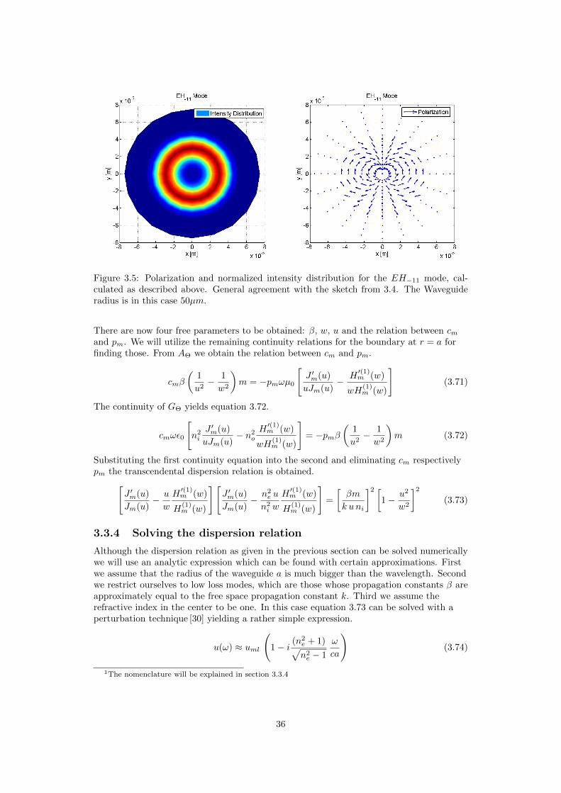
Figure 3.5: Polarization and normalized intensity distribution for the EH−11 mode, cal-culated as described above. General agreement with the sketch from 3.4. The Waveguideradius is in this case 50µm.

There are now four free parameters to be obtained: β, w, u and the relation between cmand pm. We will utilize the remaining continuity relations for the boundary at r = a forfinding those. From AΘ we obtain the relation between cm and pm.

cmβ

(1

u2− 1

w2

)m = −pmωµ0

[J ′m(u)

uJm(u)− H

′(1)m (w)

wH(1)m (w)

](3.71)

The continuity of GΘ yields equation 3.72.

cmωε0

[n2i

J ′m(u)

uJm(u)− n2

o

H′(1)m (w)

wH(1)m (w)

]= −pmβ

(1

u2− 1

w2

)m (3.72)

Substituting the first continuity equation into the second and eliminating cm respectivelypm the transcendental dispersion relation is obtained.[

J ′m(u)

Jm(u)− u

w

H′(1)m (w)

H(1)m (w)

][J ′m(u)

Jm(u)− n2

e u

n2i w

H′(1)m (w)

H(1)m (w)

]=

[βm

k uni

]2 [1− u2

w2

]2

(3.73)

3.3.4 Solving the dispersion relation

Although the dispersion relation as given in the previous section can be solved numericallywe will use an analytic expression which can be found with certain approximations. Firstwe assume that the radius of the waveguide a is much bigger than the wavelength. Secondwe restrict ourselves to low loss modes, which are those whose propagation constants β areapproximately equal to the free space propagation constant k. Third we assume therefractive index in the center to be one. In this case equation 3.73 can be solved with aperturbation technique [30] yielding a rather simple expression.

u(ω) ≈ uml

(1− i (n2

e + 1)√n2e − 1

ω

ca

)(3.74)

1The nomenclature will be explained in section 3.3.4

36

Where uml is the l-th root of the equation 3.75. The usually encountered formulation is

u(k) ≈ uml(

1− i (n2e+1)√n2e−1

1ka

). This formulation is more convenient as typically one thinks

in wavelengths rather than in frequencies.

Jm−1(uml) = 0 (3.75)

With the relations

k2i = n2

i k2 − β2 (3.76)

k2e = n2

ek2 − β2 (3.77)

where ki = ua and ke = w

a are the transversal wave numbers. This explains then thenotation used earlier, EHml refers to the mode with a modeparmeter m and a transversalwavenumber according to the l-th root of Jm−1.We finally have all the parameters we need to fully specify our modes. Inserting thedispersion relation into equation 3.76 and Taylor expanding twice we find the expressionfor β.

βml(ω) ≈ k

[1− 1

2

(umlωca

)2(

1− i (n2e + 1)√n2e − 1

2ω

ca

)](3.78)

We see, if we rewrite the above equation in terms of the wavelength that it depends on(λa )2. That means that for a� λ the axial wavenumber β → k. This is the intuitive resultwe would expect as free space can be interpreted as a special case of a waveguide withinfinite diameter. Anyhow it also allows us to calculate only fundamental as beingpropagated in modes while calculating the high harmonics in free space. Because withincreasing harmonic order the ratio (λa )2 will decrease until almost no mode properties areto be expected.

βml(λ) ≈ k

[1− 1

2

(uml2π

)2(λ

a

)2(

1− i (n2e + 1)

π√n2e − 1

λ

a

)](3.79)

Now having βml from the equation above we can calculate u and w. Having u and w, ~Aand ~G is fully specified. Anyhow as the only restrictions given for l and m are that theyare integer numbers we are dealing with an infinite set of solutions. Keeping in mind, thatwe solved the problem only for a delta shaped frequency spectrum, the complete solutionto the problem is of the shape:

~E(r,Θ, z, t) =∑ml

cml ~Aml(r,Θ, ω) exp(iωt− i βml)(ω) z) (3.80)

~H(r,Θ, z, t) =∑ml

dml ~Gml(r,Θ, ω) exp(iωt− i βml(ω) z) (3.81)

Therefore the whole mode propagation problem for a defined wavelength and fiberdiameter is solved once the cml are defined.

3.3.5 Coupling power into the waveguide

The question of how big the individual cml is again a question of the boundary conditions.We assume that we are at t = 0, z = 0 and there is a incident field ~Einc(r,Θ) on the waveguide entrance. The Bessel functions constitute a full basis in two dimensions [31]. Thatallows us to require

37

~Einc(r,Θ) =∑ml

cml ~Aml(r,Θ, ω) (3.82)

The Bessel functions are by definition orthogonal but not orthonormal. The latter requiresus to re normalize the overlap integral so that the cml are given by

cml =

∫~E∗inc · ~Amlr dr dΘ√∫~A∗ml

~Aml r dr dΘ(3.83)

We can move the division into the integral, which represents then a normalization of theradial function. From now on we require the ~A∗ml to be normalized so that∫~A∗ml

~Aml r dr dΘ = 1. By doing so the cml just become the scalar product of the two fielddistributions.

cml =

∫~E∗inc(r,Θ) · ~Aml(r,Θ)r dr dΘ (3.84)

Lets now try to extend this principle to a time dependent electric field. For example aGaussian laser pulse in space and time is given by

~E(r,Θ, t) = ~E0 exp

(− r

2

σ2

)exp

(− t

2

τ2

)exp (iω0t− ikz) (3.85)

Due to its definition, the envelope function can be separated into a purely scalar timedependence and a radial part.

~E(r, θ, t) = U(t) ~E0(r,Θ) exp (iω0t− ikz) (3.86)

Extending equation 3.82 to a time dependent case has a very peculiar problem. As soon asthe electrical field contains multiple frequencies we would have to consider individualmodes for each frequency and this is exactly the case for the laser pulse described above.The way to circumvent this complication is to assume the mode pattern ~Aml(r,Θ, ω) to be

approximately ~Aml(r,Θ, ω0) where ω0 is the center frequency of the impending electricalfield. Figure 3.6 shows the dependency of the coupling coefficient of the dominant modesexcited by a Gaussian beam. It can be seen, that in the marked area between 100 and 1000nm there is no significant change visible for the three modes with biggest contained energy.The coupling of the EH−11 mode is although exponentially increasing still one order ofmagnitude smaller than for instance the EH13 mode. This justifies the assumption takenabove. It has to be pointed out, that the approximations done in the derivations require1� λ

a , therefore the data for λa ≥ 0.1 should be considered as inaccurate.

U(t) ~E0(r,Θ) exp (iω0t) =∑ml

cml ~Aml(r,Θ, ω0) exp (iωt) (3.87)

The final representation is the very simple as every mode will have in this case exactly thesame time dependence as the initial pulse had. Which directly implies that the Fouriertransform of initial envelope function and mode envelope functions are identical up to aconstant factor.

cml(t) = U(t)

∫~E∗0 (r,Θ) · ~Aml(r,Θ, ω0) r dr dΘ (3.88)

This procedure anyhow only works as long as the time dependence is a purely scalarmultiplication. As soon as the incident field changes its radial or angular behavior in timethe above does not apply.

38

Figure 3.6: Coupling coefficients for an incident Gaussian beam of width σ on a hollow corecapillary of radius a = 50e-6m. The Gaussian beam is incident centered on the fiber. Theincident field has a normalized power of 1.

3.4 Mode propagation of the Fundamental

3.4.1 The envelope formalism for mode propagation

The goal of the next few pages is to sketch how to obtain a set of scalar equations,describing the mode propagation of the fundamental. From the previous discussion ofsolutions for the optical waveguide we know that the electric field propagates in modeswithin the waveguide. The electrical field of a light pulse with a defined envelope can thenbe written analogously to the free space case as the sum of the modes times a individualscalar envelope function Un. This was proven in the previous section for a Gaussian pulsebut it can be shown in general. [32] Consider a pulse with a center frequency of ω0:

~E(~r, t) =∑n

Vn(z, t) ~An(r,Θ) exp (iω0t) (3.89)

Respectively in Fourier space

~E(~r, ω) =∑n

Vn(z, ω − ω0) ~An(r,Θ) (3.90)

3.4.2 The envelope equation for mode propagation

In the further discussion of envelope equations, whenever there is a mode distribution~An(r,Θ), it always refers to ~An(r,Θ, ω0). This is possible because we have shownpreviously that the overlap integrals and therefore indirectly the mode patterns do notsignificantly change in our region of interest if we allow ~A to be frequency dependent. Theidea is now to use the envelope representation of the electric field together with thepropagation equation in frequency space for the fundamental (Eq. 3.5). By exploiting the

orthonormality of the radial functions (see 3.3.5) ~An(r,Θ) we obtain n scalar equations,where n is the number of modes. For convenience we introduce here a Dirac like notation.So ~An(r,Θ) = |An〉 where we know that

∑〈Am| An〉 = δ(m,n). Here δ(m,n) is the

Kronecker function and 〈Am| An〉 =∫∫A∗m(r,Θ)An(r,Θ) r dr dΘ. The result looks already

promising, as it resembles closely the Helmholtz equation for the free space case.

39

(∇2T +

d2

dz2)∑n

Vn(z, ω − ω0) |An〉+ω2

c2n2(ω)

∑n

Vn(z, ω − ω0) |An〉 = 0 (3.91)

Where we used the fact that ∇2 can be decomposed into (∇2T + d2

dz2 ) a transversal and anaxial part. By a projection on |Am〉 the principal goal is already achieved, we are left ofwith n scalar equations describing the propagation of the m-th mode. After some minoralgebraic modifications and assuming that βm(ω) is constant we obtain the finalpropagation equations 3.92.

∑n

〈Am| ∇2T |An〉 Vn(z, ω − ω0) +

∂2

∂z2Vn(z, ω − ω0) + β2

n(ω)Vn(z, ω − ω0) = 0 (3.92)

3.4.3 The paraxial scalar mode propagation equation

A small set of further approximations reduces the mathematical complications required tosolve the propagation equations considerably. The first thing to be considered is thetransverse gradient matrix element 〈Am| ∇2

T |An〉 appearing in the first term of equation3.92. In general |Am〉 would be a function of z, as we know experimentally that there willbe plasma formation within the waveguide. It significantly changes the boundaryconditions and thereby the solutions to the maxwell equation. Anyhow already byassuming βm(ω) to be constant we assume the solutions to be invariant in z. Thereforewithin this approximation the transverse gradient matrix element will also be invariant inz.It turns out that we can completely neglect the first term. Anyhow the argument is a bitmore subtle. From the definition of the Matrix element and assuming ∇T to be forCartesian coordinates we obtain an integral form.

〈Am| ∇2T |An〉 =

∫∫A∗m(x, y)

(d2

dx2+

d2

dy2

)An(x, y) dx dy (3.93)

Now as the modal field distributions drops to zero at the boundaries of integration, it canbe shown that it does not matter which function to differentiate.∫

g′(x) f(x) dx = [f(x) g(x)]Boundary −∫g(x) f(x) dx (3.94)

We introduce now 〈A′| = ∇2T A∗m(r,Θ). Therefore the transverse gradient matrix element

becomes 〈A′m| An〉. Now lets look at the first term of equation 3.92 again and try to find aupper boundary for the expression.∑

n

〈A′m| An〉 Un(z, ω − ω0) (3.95)

As shown in the next subsection the envelope functions Un are related to the fractionalpower in each mode. Therefore the sum of the squares of the envelope functions can berenormalized to one. Which leaves us with an interesting inequality.∣∣∣∣∣∑

n

〈A′m| An〉 Un(z, ω − ω0)

∣∣∣∣∣ ≤∣∣∣∣∣∑n

〈A′m| An〉

∣∣∣∣∣ (3.96)

Now the right hand side in equation 3.96 represents nothing but a projection onto thebasis of our normalized mode distributions, which is an unitary operation. Therefore wehave proven that the whole expression given above must be smaller than |∇2

T Am|.Therefore as long as the variation in transversal direction is small compared to thevariation of the electric field in axial direction the whole term involving the transverse

40

gradient matrix element can be neglected. This is called the paraxial approximation. In ourcase the variation of the mode pattern is on a characteristic scale of the fiber diameterwhile the variation in axial direction is on the scale of the wavelength, the approximationseems thereby reasonable. An interesting side effect is that by dropping this term theequation system is also automatically uncoupled, meaning that the evolution of theindividual modes is not influenced by each other.After having applied all of the approximations introduced above the initial set of coupledsecond order differential equations become a set of independent homogeneous first orderdifferential equations that we have seen already in 3.1.3.

∂2

∂z2Vn(z, ω − ω0) = −β2

n(ω)Vn(z, ω − ω0) (3.97)

Which has the solutions:

Vn(z, ω − ω0) = Un(ω − ω0) exp (−iβn(ω)z) (3.98)

As we would expect the obtained equations converge to the free space envelope equation(Eq. 3.14) for the case of r →∞ as then βm(ω0)→ k(ω0) and βm(ω)→ k(ω0). As a finalstep we introduce the co-propagating frame for each of the modes.

Vn(z, ω − ω0) = Un(ω − ω0) exp (−i [βn(ω)− βn(ω0)] z) (3.99)

It has already been described how to obtain the ~U(t) (see 3.3.5) for our purpose. The

quantity ~Un(ω − ω0) occurring here is just the Fourier transform of the initial one shiftedto be centered in frequency around zero. We are now left with basically an infinite set ofequations that all need to be solved in order to obtain the electric field at each position inspace. Anyhow the next section will deal with how to limit the amount of to be consideredmodes.

3.4.4 The active mode approximation

In the previous section it was shown that for our conditions the transverse gradient termcan be neglected. Therefore there will be no coupling of energy between the individualmodes during the propagation (see eq 3.92), as already in the very beginning only linearpropagation was assumed. This again means that we have to consider in the propagationonly the modes that the incident field on the fiber entrance couples to. Restrictingourselves to the case where the incident field is linearly polarized and Gaussian in space antime, we find that there is only a few modes that actually have to be taken into account.Figure 3.7 displays the mode coupling of a Gaussian beam for different modes for a definedσa .Repeating these simulations for various values of σ

a we find that for a region around σa =

0.64 more than 98% of the power is coupled into the EH11 mode. Figure 3.8 shows thesimulations on how the focal size of the incident gaussian beam affects the couplingcoefficient of the dominant modes. Said figure has two interesting features; it not onlyshows that for the right focusing conditions almost all power is coupled into a distinctmode, it also shows that for a broad range of 0.3 > σ

a > 0.7 that the first three of theEH1m cover almost 100% of the guided power.The conclusion here is that it is sufficient in the conditions assumed here, to consider onlythe EH1m modes and of those also only the lower orders. The conclusion that has beenreached above in a purely mathematical way can be qualitatively explained by looking atfigure 3.4 and reminding ourselves that by calculating the coupling coefficient we calculatethe mode overlap integral between the incident field and the particular mode. The EH1m

modes are the only modes that are linearly polarized and therefore show the biggestoverlap with our initially linearly polarized Gaussian beam. The active modeapproximation is also the reason why we were allowed to neglect the TE and TM modes

41

Figure 3.7: Coupling coefficients for a incident Gaussian beam of width σ on a hollow corecapillary of radius a = 50e-6m. The Gaussian beam is incident centered on the fiber. For thisratio of σ

a there seems to be only coupling into the lower orders of the EH1m and EH−1m

modes. The sum of all |cmn|2 displayed here is 0.97, for an electric field with normalizedpower 1.

Figure 3.8: Coupling coefficients of the dominant modes of a incident Gaussian beam ofwidth σ on a hollow core capillary of radius a = 50e-6m. The Gaussian beam is incidentcentered on the fiber. For σ

a = 0.64 the coupling efficiency is about 98%.

42

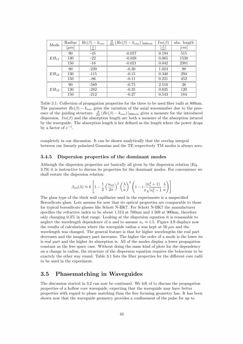
ModeRadius Re(β)− kvac ∂

∂λ (Re(β)− kvac) |800nm Im(β) abs. length[µm] [ 1

m ] [ 1m ] [cm]

EH11

90 -45 -0.057 0.194 515130 -22 -0.028 0.065 1538150 -16 -0.021 0.042 2381

EH12

90 -239 -0.30 1.024 98130 -115 -0.15 0.340 294150 -86 -0.11 0.221 452

EH13

90 -589 -0.75 2.516 38130 -282 -0.35 0.835 120150 -212 -0.27 0.543 184

Table 3.1: Collection of propagation properties for the three to be used fiber radii at 800nm.The parameter Re(β) − kvac gives the variation of the axial wavenumber due to the pres-ence of the guiding structure. ∂

∂λ (Re(β)− kvac) |800nm gives a measure for the introduceddispersion. Im(β) and the absorption length are both a measure of the absorption intucedby the waveguide. The absorption length is her defined as the length where the power dropsby a factor of e−1.

completely in our discussion. It can be shown analytically that the overlap integralbetween our linearly polarized Gaussian and the TE respectively TM modes is always zero.

3.4.5 Dispersion properties of the dominant modes

Although the dispersion properties are basically all given by the dispersion relation (Eq.3.79) it is instructive to discuss its properties for the dominant modes. For convenience weshall restate the dispersion relation:

βml(λ) ≈ k

[1− 1

2

(uml2π

)2(λ

a

)2(

1− i (n2e + 1)

π√n2e − 1

λ

a

)]The glass type of the thick wall capillaries used in the experiments is a unspecifiedBorosilicate glass. Lets assume for now that its optical properties are comparable to thosefor typical borosilicate glasses like Schott N-BK7. For Schott N-BK7 the manufacturerspecifies the refractive index to be about 1.513 at 700nm and 1.509 at 900nm, thereforeonly changing 0.3% in that range. Looking at the dispersion equation it is reasonable toneglect the wavelength dependence of n and to assume ne ≈ 1.5. Figure 3.9 displays nowthe results of calculations where the waveguide radius a was kept at 50 µm and thewavelength was changed. The general feature is that for higher wavelengths the real partdecreases and the imaginary part increases. The higher the order of a mode is the lower itsis real part and the higher its absorption is. All of the modes display a lower propagationconstant as the free space case. Without doing the same kind of plots for the dependencyon a change in radius, the structure of the dispersion equation requires the behaviour to beexactely the other way round. Table 3.1 lists the fiber properties for the different core radiito be used in the experiment.

3.5 Phasematching in Waveguides

The discussion started in 3.2 can now be continued. We left of to discuss the propagationproperties of a hollow core waveguide, expecting that the waveguide may have betterproperties with regard to phase matching than the free focusing geometry has. It has beenshown now that the waveguide geometry provides a confinement of the pulse for up to

43

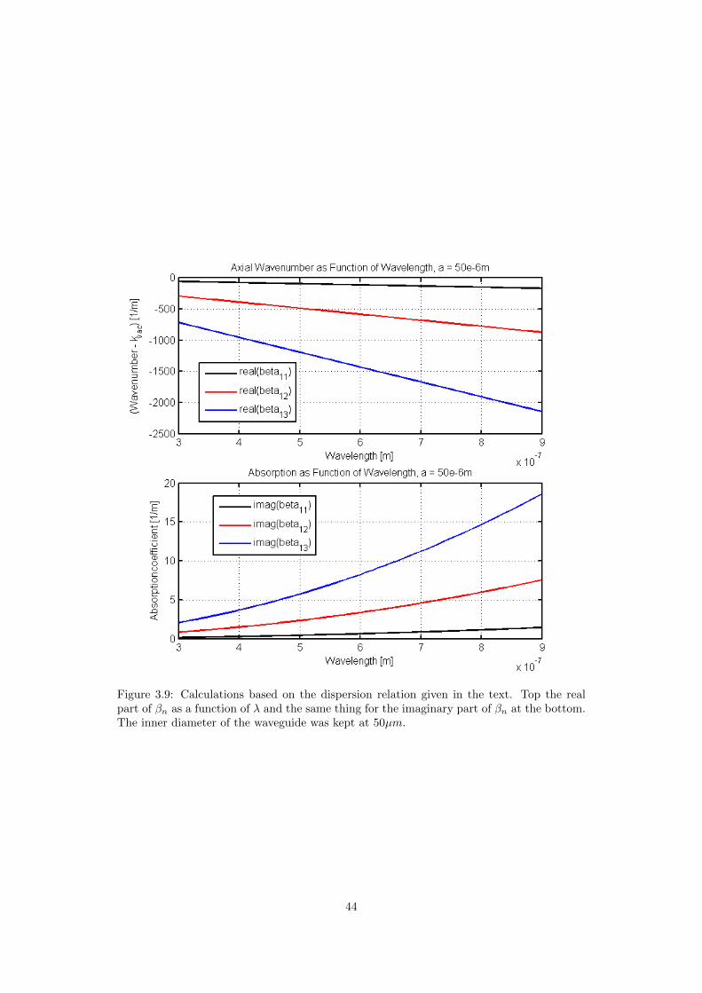
Figure 3.9: Calculations based on the dispersion relation given in the text. Top the realpart of βn as a function of λ and the same thing for the imaginary part of βn at the bottom.The inner diameter of the waveguide was kept at 50µm.

44

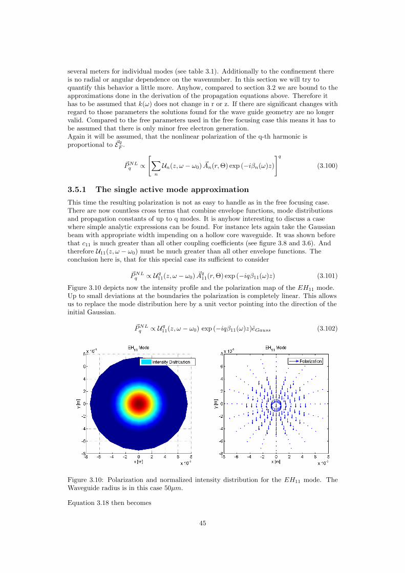
several meters for individual modes (see table 3.1). Additionally to the confinement thereis no radial or angular dependence on the wavenumber. In this section we will try toquantify this behavior a little more. Anyhow, compared to section 3.2 we are bound to theapproximations done in the derivation of the propagation equations above. Therefore ithas to be assumed that k(ω) does not change in r or z. If there are significant changes withregard to those parameters the solutions found for the wave guide geometry are no longervalid. Compared to the free parameters used in the free focusing case this means it has tobe assumed that there is only minor free electron generation.Again it will be assumed, that the nonlinear polarization of the q-th harmonic isproportional to ~EqF .

~PNLq ∝

[∑n

Un(z, ω − ω0) ~An(r,Θ) exp (−iβn(ω)z)

]q(3.100)

3.5.1 The single active mode approximation

This time the resulting polarization is not as easy to handle as in the free focusing case.There are now countless cross terms that combine envelope functions, mode distributionsand propagation constants of up to q modes. It is anyhow interesting to discuss a casewhere simple analytic expressions can be found. For instance lets again take the Gaussianbeam with appropriate width impending on a hollow core waveguide. It was shown beforethat c11 is much greater than all other coupling coefficients (see figure 3.8 and 3.6). Andtherefore U11(z, ω − ω0) must be much greater than all other envelope functions. Theconclusion here is, that for this special case its sufficient to consider

~PNLq ∝ Uq11(z, ω − ω0) ~Aq11(r,Θ) exp (−iqβ11(ω)z) (3.101)

Figure 3.10 depicts now the intensity profile and the polarization map of the EH11 mode.Up to small deviations at the boundaries the polarization is completely linear. This allowsus to replace the mode distribution here by a unit vector pointing into the direction of theinitial Gaussian.

~PNLq ∝ Uq11(z, ω − ω0) exp (−iqβ11(ω)z)eGauss (3.102)

Figure 3.10: Polarization and normalized intensity distribution for the EH11 mode. TheWaveguide radius is in this case 50µm.

Equation 3.18 then becomes

45

∆k = kq − qβ11 (3.103)

3.5.2 Neutral gas dispersion in waveguides

The rest of this section will closely resemble the discussion in section 3.2, just that thistime the wave guide geometry is considered. All the quantities introduced there will not beintroduced again here, in case of doubt please refer to section 3.2.

The dispersion relation 3.79 can be written in a slightly different form

βml(λ) ≈ k [1− εml(λ, a)] (3.104)

In the initial reference [30] it was assumed that the inner refractive index in the waveguideis one, k in the expression above represents then the vacuum wavenumber. Anyhow theinner refractive index can be treated as a perturbation to this case. Therefore we obtain anequation, consistent with the free space derivations.

βml(ω) ≈ kvacF nF [1− εml(λ, a)] (3.105)

This expression has the expected asymptotic behavior for aλ →∞ respectively ε→ 0.

∆k = qkvacF (nq − nF [1− εml]) (3.106)

which is clearly positive as nq > 1. The rest of the derivation works analogously to the freefocusing case and leads to an almost identical expression.

∆kN = qkFP

Patm(1− η) (nq − nF [1− εml]) (3.107)

It follows that for small εml the sign of ∆kN remains positive for the same reasons as givenin 3.2.1.

3.5.3 Free electron dispersion in waveguides

Using equations 3.28 and 3.106 an analogous expression to 3.29 is obtained.

∆ke = qkFNe2

2mε0

[1

ω2F

− 1

ω2q

− εml(

2mε0Ne2

− 1

ω2F

)](3.108)

Which can be rewritten to

∆ke = qkFNe2

2mε0

[1 + εmlω2F

− 1

ω2q

]− εmlqkF (3.109)

Or in a form similar to 3.30

∆ke = qkFNatmP

Patm

e2

2mε0ω2F

[(1 + εml)q

2 − 1

q

]− εmlqkF (3.110)

As εml is assumed to be small, ∆ke is still positive.

3.5.4 The dipole phase in waveguides

The discussion of the dipole phase in waveguides is completely analogous to the discussionin the free focusing geometry. This is not surprising, as within the atomic process nothinghas changed. Therefore the dipole phase term behaves the same way in both geometries.

46

3.5.5 Conclusion of the phasematching properties

Collecting all the ∆k terms obtained for the various contributions again we find an almostidentical relation as before. The only differences are that the Gouy term disappeared andthat ∆kN and ∆ke are additionally dependent on the inner diameter of the waveguide.

∆kwaveguidetotal = ∆kN (q, λF , a, P, η) + ∆ke (q, λF , a, P, η) + ∆kdipole (q, I) (3.111)

Therewith all the problems pointed out in 3.2.5 have been resolved. First, the phasematching does no longer depend on the focusing conditions while the intensity is conservedover much longer distances than possible in a reasonable free focusing geometry (see table3.1. Second it seems much more feasible to maintain a defined pressure over such a longdistance within a fiber than within free space. Third we found an additional free parameterthat can be experimentally tweaked. Anyhow there are some drawbacks. Foremost, thederivation only allows ionization fractions much smaller than one. Also there is still aradial dependence of the phase, caused by the fact that the intensity is a function of theradius. If it was possible to find a fiber geometry that fulfills all the previous requirementsthat we demanded to get to this point, and additionally provides a dominant Eigen modewith a very low intensity gradient in the center, an almost perfect HHG geometry wouldhave been found. To illustrate this, figure 3.11 shows the radial dependence of theintensity for a Gaussian field distribution and a J0 field distribution as for the EH11 mode.One can imagine more sophisticated fiber geometries with flat top like profiles.

Figure 3.11: Radial dependence of the intensity for a Gaussian, J0 and J1 field distribution.All functions are normalized to the same area. The width of the Gaussian is chosen suchthat sigma

a = 0.64, representing the optimal coupling conditions for the EH11 mode.

3.6 Conclusion on Chapter 3

In this chapter the mathematical and physical tools required to do simple calculations onhigh harmonic generation in hollow core capillaries have been introduced, motivated andproven as far as possible. Same goes for the approximations and assumptions done in theprocess of finding these tools. The solution strategy for the propagation of a simpleGaussian pulse should now be clear. It can be summarized as follows.

1. Calculate propagation of fundamentala) find modesb) decompose pulse into mode envelope functionsc) single out the dominant modesd) transform envelope functions to frequency spacee) propagate with envelope equation

47

2. Calculate propagation of harmonica) get nonlinear polarization from fundamentalb) propagate with envelope equationc) transform result back into time space

Additional to this, analytic considerations on the phase matching condition and coherentbuildup of high harmonics were presented. The important points there are, that thepossible phase matching volume is considerably higher than everything that can beachieved with a free focusing geometry while getting rid of the Gouy phase contribution.The fundamentally different intensity distributions that can be encountered in this verysimple case of a wave guide should hint at possible further application with tailoredwaveguides to achieve even higher phase matching volumes and conversion efficiencies.Finally, it must be kept in mind that in developing this formalism a couple of strongapproximations have been made. The linearization of the propagation equations and theBorn approximation (see: 3.1.2) most notably. This example was picked for the reason,that it is known that lower order harmonics contribute significantly to the high orderharmonic generation process itself. Anyhow this is beyond the scope of the simpletheoretical considerations that the author wanted to present here. It was the goal tomaintain as much generality as necessary to motivate the experiment suggested in the nextchapter. For more meticulous and general derivations see [37, 36] for short pulsepropagation in general and [38, 39] for propagation equations in fibers with present plasma.There are also several classical papers dealing with propagation of high harmonics anyhowusing more complicated derivations in time space [13, 14, 16] and in particular [4].

48

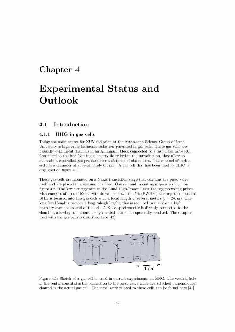
Chapter 4

Experimental Status andOutlook

4.1 Introduction

4.1.1 HHG in gas cells

Today the main source for XUV radiation at the Attosecond Science Group of LundUniversity is high-order harmonic radiation generated in gas cells. These gas cells arebasically cylindrical channels in an Aluminum block connected to a fast piezo valve [40].Compared to the free focusing geometry described in the introduction, they allow tomaintain a controlled gas pressure over a distance of about 1 cm. The channel of such acell has a diameter of approximately 0.5 mm. A gas cell that has been used for HHG isdisplayed on figure 4.1.

These gas cells are mounted on a 5 axis translation stage that contains the piezo valveitself and are placed in a vacuum chamber. Gas cell and mounting stage are shown onfigure 4.2. The lower energy arm of the Lund High-Power Laser Facility, providing pulseswith energies of up to 100 mJ with durations down to 45 fs (FWHM) at a repetition rate of10 Hz is focused into this gas cells with a focal length of several meters (f = 2-6 m). Thelong focal lenghts provide a long raleigh lenght, this is required to maintain a highintensity over the extend of the cell. A XUV spectrometer is directly connected to thechamber, allowing to measure the generated harmonics spectrally resolved. The setup asused with the gas cells is described here [42].

Figure 4.1: Sketch of a gas cell as used in current experiments on HHG. The vertical holein the center constitutes the connection to the piezo valve while the attached perpendicularchannel is the actual gas cell. The intial work related to these cells can be found here [41].

49

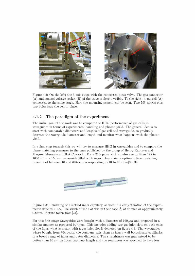
Figure 4.2: On the left: the 5 axis stage with the connected piezo valve. The gas connector(A) and control voltage socket (B) of the valve is clearly visible. To the right: a gas cell (A)connected to the same stage. Here the mounting system can be seen. Two M3 screws plustwo bolts keep the cell in place.

4.1.2 The paradigm of the experiment

The initial goal of the work was to compare the HHG performance of gas cells towaveguides in terms of experimental handling and photon yield. The general idea is tostart with comparable diameters and lengths of gas cell and waveguide, to graduallydecrease the waveguide diameter and length and monitor what happens with the photonyield.

In a first step towards this we will try to measure HHG in waveguides and to compare thephase matching pressures to the ones published by the group of Henry Kapteyn andMargret Murnane at JILA Colorado. For a 23fs pulse with a pulse energy from 125 to1640µJ in a 150µm waveguide filled with Argon they claim a optimal phase matchingpressure of between 10 and 60 torr, corresponding to 10 to 70 mbar[33, 34].

Figure 4.3: Rendering of a slotted inner capillary, as used in a early iteration of the experi-ments done at JILA. The width of the slot was in their case 1

32 of an inch or approximately0.8mm. Picture taken from [34].

For this first stage waveguides were bought with a diameter of 160µm and prepared in asimilar manner as proposed by them. This includes adding two gas inlet slots on both endsof the fiber, what is meant with a gas inlet slot is depicted on figure 4.3. The waveguideswhere bought from Vitrocom, the company sells them as heavy wall borosilicate capillariesin a broad range of inner and outer diameters. The straightness was guaranteed to bebetter than 10µm on 10cm capillary length and the roundness was specified to have less

50

than 3.5µm deviation from the circle for a 0.150µm inner diameter capillary. The slotswere added by Scientific Lab Glass Lund AB with a diamond disc saw. Figure 4.4 showsone of our capillaries prepared with the gas inlet slot.

Figure 4.4: Vitrocom HWC010-55 heavy wall capillary with added gas inlet slot. The slotwidth is about 2 mm.

4.2 Design and Development of the Fiber Mount

Having the fibers, a suitable mount was needed that allowed to deliver the appropriatebacking pressure to the gas inlets, while not leaking any unnecessary gas into the vacuum.There were different fairly advanced designs by other groups, most notably the V-groovemount presented in Ariel J. Pauls thesis[34]. However the design presented here deviatessignificantly from any of those, due to being adapted particularly for our vacuum systemand the given manufacturing possibilities.

4.2.1 Development considerations

In order to allow an easy and uncomplicated change between gas cells and waveguides thewaveguide mount needed to be compatible with the gas cell mounting system, thereforehave the same sort of attachment points as the gas cells have (see figure 4.2). Furthermore,it should be possible to mount and unmount the wave guide system without needing toremove the translation stage from the vacuum chamber. This implies that all the screwsthat need to be unscrewed for removing the mount should be accessible from the top.

Another feature that was required from the mount was to support variable waveguidelengths and allow variable inlet positions, while at the same time the center piece of thewaveguide should be visible from the top in order to support the alignment procedure andto allow direct monitoring of the processes inside. Also for alignment reasons it wasnecessary, that the waveguide entrance can be located at the same position as the gas cellentrance, as this is the center of rotation for the 5-way gas cell holder. Positions differentfrom that would complicate the alignment procedure significantly.

4.2.2 The design

The design we came up with was then a modification of a mount presented by F. Wojda inhis thesis [43]. It relies on two gas delivery end pieces that the waveguide is glued in with asilicone glue.1 These two end pieces can then be moved relative to each other in a rail,

1So far we have not tried to mount the system with an actual waveguide, anyhow the glue that we planto use will be Loctite AS 310. This type of silicone clue is vacuum compatible and was recommended forthis purpose by other groups.

51

allowing changing inlet positions and waveguide lengths. The end piece design is shown infigure 4.5.

Figure 4.5: The end piece for the waveguide mount. The gas streams in through the topinto the volume in the center where the gas inlets of the waveguide are positioned. A lid isscrewed on top of the end piece, that allows to seal the volume from both sides with siliconeglue.

The easy mounting and un-mounting issue was solved by having a separate mounting plateto which the rail was fixed by two M3 screws. This mounting plate has the screws andbolts layout as the gas cell has and can thus be attached on top of the piezo valve just likethe cell. The piezo valve can then be used to control the gas flow into the waveguide. Thefinal mount is presented in figure 4.6. It fulfills all the requirements given. The biggestdrawback of our mount will probably be the fairly long time that is required to replace adamaged waveguide or to switch to a different waveguide in an experiment. The alignmentwill also be lost every time the waveguide is changed. However, it should be noted thatbreaking and re-establishing the vacuum takes the longest time in the procedure ofchanging capillaries. This is the same for all possible designs.

Figure 4.6: On the left: the final design for the capillary holder. The two end pieces canbe moved in a rail. The rail itself can be easily unscrewed from the mounting plate in theback. On the right: the assembly with the gas connectors attached. The lids for the endpieces are missing in this picture.

52

4.3 Calculations on Pressure Dynamics

As it was shown in chapter 3, the pressure distribution plays a significant role in the phasematching for HHG. The choice of a hollow core wave guide can also be justified solely bythe possibility of providing a constant gas pressure over almost arbitrary distances.However, there is the technical boundary condition that the current gas supply is built todeliver a pulsed gas jet as described earlier in this chapter. Therefore the system layout isdesigned for delivering gas flow to a completely different geometry. It needs to beinvestigated, whether a pulsed backing pressure for the waveguides is feasible in terms ofthe expected time constants and expected gas flow. The aim of modelling the gas flow is toobtain an order of magnitude estimation of the required parameters for the opening timeof the piezo valve and the overall backing pressure.

4.3.1 Modeling of the gas flow

The first step in the process of modeling the gas flow is to ecompose the geometry into aset of volume elements of constant circular cross section at constant pressure.

Figure 4.7: 1D waveguide model. Decomposition of the geometry into volume elements ofconstant circular cross sections at constant pressure.

The gasflow can then be modelled rather easily, if the following assumptions apply:

1. The flow can be considered laminar.2. The fluid is approximately incompressible.3. The flow is through a constant circular cross section.4. The circular cross crossection is significantly longer than its diameter.

The volumetric flow Φ = ∂V∂t ≈

∆V∆t is given by the Hagen-Poiseille equation [44]:

Φ =∆P

∆x

πR4

8η(4.1)

where R is the radius of the volume elements and η represents the viscosity. Its clear thatthe conditions 3. and 4. are fulfilled or can be easily fulfilled by the choice of calculationparameters. 2. can be dropped by taking the obtained results as boundary values, meaningthat we overestimate the flux and underestimate the time constants significantly. Thismeans, that the actual flux might be an order of magnitude lower, while the actual timeconstant might be an order of magnitude higher. This approximation is bold, as a noblegas is naturally highly compressible, however for checking the order of magnitude it issufficient. We continue here with the ad hoc assumption that the predominant flow in such

53

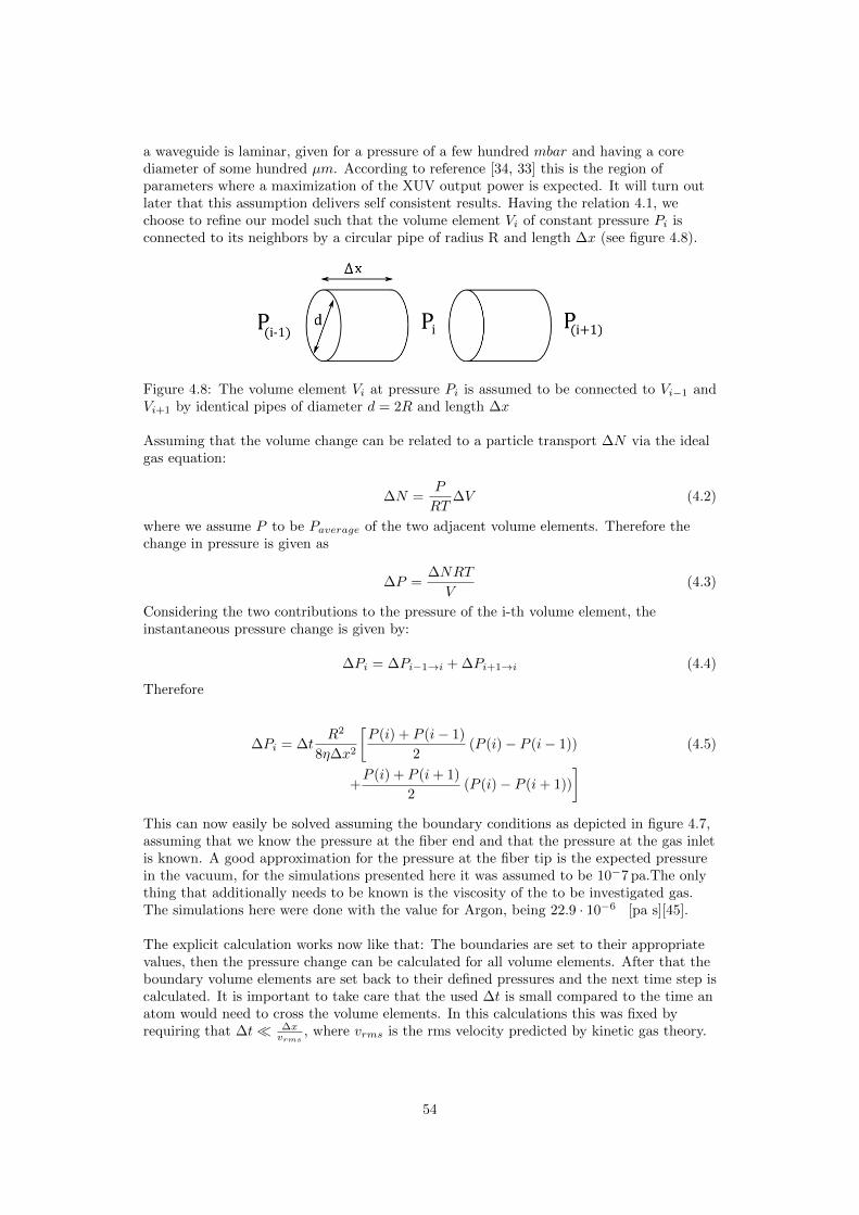
a waveguide is laminar, given for a pressure of a few hundred mbar and having a corediameter of some hundred µm. According to reference [34, 33] this is the region ofparameters where a maximization of the XUV output power is expected. It will turn outlater that this assumption delivers self consistent results. Having the relation 4.1, wechoose to refine our model such that the volume element Vi of constant pressure Pi isconnected to its neighbors by a circular pipe of radius R and length ∆x (see figure 4.8).

Figure 4.8: The volume element Vi at pressure Pi is assumed to be connected to Vi−1 andVi+1 by identical pipes of diameter d = 2R and length ∆x

Assuming that the volume change can be related to a particle transport ∆N via the idealgas equation:

∆N =P

RT∆V (4.2)

where we assume P to be Paverage of the two adjacent volume elements. Therefore thechange in pressure is given as

∆P =∆NRT

V(4.3)

Considering the two contributions to the pressure of the i-th volume element, theinstantaneous pressure change is given by:

∆Pi = ∆Pi−1→i + ∆Pi+1→i (4.4)

Therefore

∆Pi = ∆tR2

8η∆x2

[P (i) + P (i− 1)

2(P (i)− P (i− 1)) (4.5)

+P (i) + P (i+ 1)

2(P (i)− P (i+ 1))

]This can now easily be solved assuming the boundary conditions as depicted in figure 4.7,assuming that we know the pressure at the fiber end and that the pressure at the gas inletis known. A good approximation for the pressure at the fiber tip is the expected pressurein the vacuum, for the simulations presented here it was assumed to be 10−7 pa.The onlything that additionally needs to be known is the viscosity of the to be investigated gas.The simulations here were done with the value for Argon, being 22.9 · 10−6 [pa s][45].

The explicit calculation works now like that: The boundaries are set to their appropriatevalues, then the pressure change can be calculated for all volume elements. After that theboundary volume elements are set back to their defined pressures and the next time step iscalculated. It is important to take care that the used ∆t is small compared to the time anatom would need to cross the volume elements. In this calculations this was fixed byrequiring that ∆t� ∆x

vrms, where vrms is the rms velocity predicted by kinetic gas theory.

54

4.3.2 Temporal pressure evolution

The information that we want is whether or not the time constants involved in thepressure dynamics are comparable with the time constant of the consecutive laser pulses(100 ms) and in what order of magnitude the gas flux is that escapes into the vacuum.Figure 4.9 and 4.10 display the results of two example calculations. It is apparent that thetime constant τ for reaching a steady state is one order lower than the laser repetitionrate. According to this calculations, it would not yet be a problem for a fiber length of 6cm with τ being in the order of 2.5 ms. Already for 8 cm fiber length τ is much larger than5 ms for 80 µm fiber radius. Anyhow it has to be kept in mind that we underestimate thetime constant, therefore it is reasonable to assume that the real time constants are infactlonger than 10ms and be therefore in the order of the temporal pulse separation.Calculations including the compressibility of the investigated gas need to be done forclarification.

Figure 4.9: Pressure dynamics for Argon in a 6 cm waveguide with a core radius of R =80µm

It was stated before that these simulations are self consistent in terms of the laminar flowassumption. This can be shown using the condition that the Reynolds Re number is atany time smaller than a boundary value Recrit. For flow in a pipe this value is about2000 [46]. The Reynolds number is now calculated as

Re =vR

ηρ (4.6)

where v is the mean velocity of the atoms in the gas, R the radius of the pipe and ρ is thedensity of the gas. The above can be rewritten using Hagen-Poiseille formula form before.

Re(i) =r3

8η2∆x

M

RT∆Pi Paverage (4.7)

here r was used for the radius in order to allow R as universal gas constant, M denotes themolar mass. Therewith we can plot a Reynolds map of every point in space and time andcompare these values to Recrit. Figure 4.11 shows these calculations for the data fromfigure 4.10.The result here is, that the maximal value occurring is Remax = 300, which is obtained atthe first time step, where the boundary conditions, being step functions, can be regarded

55

Figure 4.10: Pressure dynamics for Argon in a 6 cm waveguide with a core radius of R =150µm

Figure 4.11: Reynolds map for Argon in a 6cm waveguide with a core radius of R = 150µm

56

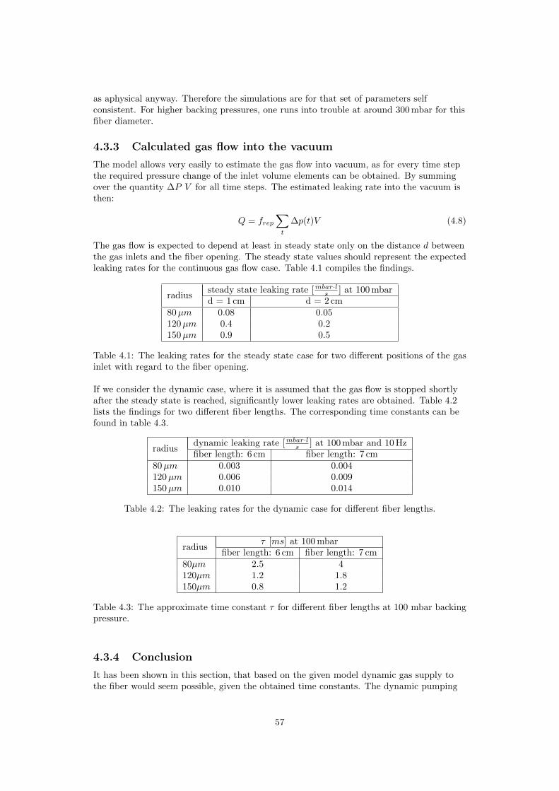
as aphysical anyway. Therefore the simulations are for that set of parameters selfconsistent. For higher backing pressures, one runs into trouble at around 300 mbar for thisfiber diameter.

4.3.3 Calculated gas flow into the vacuum

The model allows very easily to estimate the gas flow into vacuum, as for every time stepthe required pressure change of the inlet volume elements can be obtained. By summingover the quantity ∆P V for all time steps. The estimated leaking rate into the vacuum isthen:

Q = frep∑t

∆p(t)V (4.8)

The gas flow is expected to depend at least in steady state only on the distance d betweenthe gas inlets and the fiber opening. The steady state values should represent the expectedleaking rates for the continuous gas flow case. Table 4.1 compiles the findings.

radiussteady state leaking rate [mbar·ls ] at 100 mbard = 1 cm d = 2 cm

80µm 0.08 0.05120µm 0.4 0.2150µm 0.9 0.5

Table 4.1: The leaking rates for the steady state case for two different positions of the gasinlet with regard to the fiber opening.

If we consider the dynamic case, where it is assumed that the gas flow is stopped shortlyafter the steady state is reached, significantly lower leaking rates are obtained. Table 4.2lists the findings for two different fiber lengths. The corresponding time constants can befound in table 4.3.

radiusdynamic leaking rate [mbar·ls ] at 100 mbar and 10 Hzfiber length: 6 cm fiber length: 7 cm

80µm 0.003 0.004120µm 0.006 0.009150µm 0.010 0.014

Table 4.2: The leaking rates for the dynamic case for different fiber lengths.

radiusτ [ms] at 100 mbar

fiber length: 6 cm fiber length: 7 cm80µm 2.5 4120µm 1.2 1.8150µm 0.8 1.2

Table 4.3: The approximate time constant τ for different fiber lengths at 100 mbar backingpressure.

4.3.4 Conclusion

It has been shown in this section, that based on the given model dynamic gas supply tothe fiber would seem possible, given the obtained time constants. The dynamic pumping

57

would reduce the gas flow by more than an order of magnitude for the critical 300µmfibers with the biggest continuous leaking rates.

However, the first choice to run the experiment would be with continuous gas flow as it isthe most uncomplicated way to obtain a constant pressure profile. This is first of allbecause of the extenisve tubing that was required to connect the piezo valve with the fiberinlets. The timeconstants there would be dominating the system and make it very hard topredict the pressure distribution inside the fiber. Further due to the exclusion of thecompression effects, the time constants have been underestimated. To make sure, thatproper gas distributions are being reached more complicated calculations are required.Furthermore there is currently no possibility to directly measure the pressure distribution,that means in a dynamic gas flow setup there would be always a certain degree ofuncertainty if the steady state is actually reached.

Finally this means, that if we are running into trouble with the continuous gas load, itwould be better to change the pumping scheme in the vacuum chamber to a differentialone instead of playing with the pulsed gas flow, as only that way the pressure profile canbe guaranteed.

4.4 Outlook

This work sets the theoretical basis for a comparison of gas cells and hollow capillaries interms of HHG efficiency and experimental handling. The next step is obviously to performthe experiments described in this thesis. If everything proceeds according to plan therewill be beam time after the defense of this work. The most important things that need tobe worked out before data can be collected, are the adaption of the current pressuresystem to our needs and the development of an appropriate alignment procedure. Bothwill be dealt with as soon as possible.

The immediate goal is then to characterize and quantify HHG in hollow capillaries and tocompare the obtained data with literature [33, 34]. Optimum parameters in terms of pulseenergy, intensity, capillary diameter, gas pressure and gas type will be optained in amultidimensional optimisation process. From these experiments we hope to obtaininformation about the transition from free focusing to wave guiding properties.

With the experimental results at hand, detailed analysis based on the described modelswill be conducted, hopefully allowing us to draw a conclusion in favor of either the freefocusing gas cell geometry or the guided waveguide geometry.

58

Acknowledgements

The path of a human being is defined by the sum of the influences acting upon it. Withoutthe influence of a lot of people this thesis would have never been written. Without a lot ofpeople i would have never came to Sweden. Without a lot of people i would have maybeended up in a totally different profession.

I want to thank Prof. Christoph Gerz for making me understand physics, Dr. VladislavYakovlev for showing me that i might have been a bit fast with that first conclusion andProf. Anne L’Huillier for showing me that it does not matter, as long as you have funworking with it.

With the above being said, it was not less than an honor to work in the group of AnneL’Huillier. She provides an extraordinary working environment gathering an excellent setof people around her. Dr. Cord Arnold is possibly the best supervisor i could have endedup with. He left me all the freedom i needed to satisfy my curiosity while providing therequired boundaries to actually move forward. Its also hard to underestimate thecontribution of Diego Guenot to this work, he has the rare feature of having sufficientpatience and genius to make an ordinary cobblestone understand quantum field theory.Filippo Campi generously supplied the punctuation for this thesis and the mutualexchange of insanities shall not be forgotten, it was a pleasure. I also want thank EsbenWitting Larsen for the friendship and company, Piotr Rudawski for all the engineeringhelp one could possibly ever imagine, David Kroon for the mustache, Kathrin Klunder forthe music and being in general, Fernando Brizuela and Per Johnsson for their wonderfulhumor and Christoph Heyl for his patience under inquisitive questioning.

I want to thank my family. My grandmother for making the world a better place, mymother for supporting me since forever and my sister for being awesome. Without all ofthem this whole Sweden undertaking would not have been possible, financially andotherwise.

59

Bibliography

[1] Bransden and Joachain Physics of Atoms and Molecules, 2nd ed. Benjamin Cummings,2003

[2] McPherson et al. Studies of multiphoton production of vacuum-ultraviolet radiation inrare gases. J. Opt. Soc. Am. B 4, 1987

[3] Ferray, L’Huillier, Li, Lompre and Mainfray Multiple-harmonic conversion of 1064 nmradiation in rare gases. J. Phys. B: At. Mol. Opt. Phys. 21, 1988

[4] Lewenstein et al. Theory of high-harmonic generation by low-frequency laser fields.Phys. Rev. A 49(3), 1994

[5] Lewenstein, Salieres and L’Huillier Phase of the atomic polarization in high-orderharmonic generation. Phys. Rev. A 52(6), 1995

[6] Paul et al. Observation of a train of attosecond pulses from high harmonic generation.Science 292, 2001

[7] Krausz and Ivanov Attosecond Physics Reviews of Modern Physics 81, 2009

[8] Paul Corkum Plasma Perspective on Strong-Field Multiphoton Ionization. Phys. Rev.Lett. 71(13), 1993

[9] Rundquist et al. Phase-Matched Generation of Coherent Soft X-rays. Science 280, 1998

[10] von der Linde et al. Generation of high-order harmonics from solid surfaces by intensefemtosecond laser pulses. Phys. Rev. A. 52(1), 1995

[11] Xiong and Chin Tunnel ionization of potassium and xenon atoms in a high-intensityCO2 laser radiation field Sov. Phys. JETP 72(2), 1991

[12] Ivanov and Rzazewski Are free-free transitions a good basis for nonlinear optics?Journal of Modern Optics 39(12), 1992

[13] L’Huillier, Schafer and Kulander Theoretical aspects of intense field harmonicgeneration. J. Phys. B: At. Mol. Opt. Phys. 24, 1991

[14] L’Huillier, Balcou, Candel, Schafer and Kulander Calculations of high-orderharmonic-generation processes in xenon at 1064 nm. Phys. Rev. A, 46(5), 1992

[15] L’Huillier et al High-order harmonic-generation cutoff. Phys. Rev. A, 48(5), 1993

[16] Antoine et al. Theory of high-order harmonic generation by an ellyptically polarizedlaser field. Phys. Rev. A, 53(3), 1996

[17] Li, L’Huillier, Ferray, Lompre and Mainfray Multiple-harmonic generation in raregases at high laser intensity. Phys. Rev. A, 39(11), 1989

60

[18] Popmintchev et al The attosecond nonilnear optics of bright coherent X-raygeneration. Nature Photonics 4, 2010

[19] Varju et al Frequency chirp of harmonic and attosecond pulses. Journal of ModernOptics 52 (2-3), 2005

[20] Balcou et al Quantum-path analysis an phase-matching of high-order harmonicgeneration and high.order frequncy mixing processes in strong laser fields. J. Phys. B:At. Mol. Opt. Phys. 32, 1999

[21] Lena Roos Optimisation and Application of Intense High-Order Harmonic Pulses.Dissertation, 2001

[22] Salieres et al. Feynman’s Path-Integral Approach for Intense-Laser-Atom Interactions.Science 292, 2001

[23] D. M. Wolkow Uber eine Klasse von Losungen der Diracschen Gleichung. Zeitschriftfur Physik A 94(3-4), 1935

[24] Bethe and Salpeter Quantum Mechanics of One and Two Electron Atoms. Springer,1977

[25] Goldstein, Poole and Safko Classical Mechanics, 3rd ed. Addison Wesley, 2002

[26] Robert Boyd Nonlinear Optics, 3rd ed. Elsevier Science, 2008

[27] Katsunari Okamoto Fundamentals of Optical Waveguides, 2nd ed. Elsevier Science,2006

[28] Julius Stratton Electromagnetic Theory McGraw-Hill Book Company, 1941

[29] John D. Jackson Classical Electrodynamics, 3rd ed. John Wiley & Sons, 1999

[30] Marcatili and Schmeltzer Hollow Metallic and Dielectric Wave Guides for LongDistance Optical Transmission and Lasers. The Bell System Technical Journal, July1964

[31] Riley, Hobson and Bence Mathematical Methods for Physics and Engineering, 3rd ed.Cambridge Press, 2006

[32] Govind Agrawal Nonlinear Fiber Optics, 3rd ed. Academic Press, 2001

[33] Amy Lytle Phase Matching and coherence of High-Order Harmonic Generation inHollow Waveguides. Dissertation, 2008

[34] Ariel Paul Coherent EUV Light from High-Order Harmonic Generation:Enhancement and Applications to Lensless Diffraction Imaging. Dissertation, 2007

[35] Baha Saleh, Malvin Teich Fundamentals of Photonics, 2nd ed. Wiley-Interscience,2007

[36] Brabec and Krausz Nonlinear Optical Pulse Propagation in the Single-Cycle Regime.Phys. Rev. Lett. 78(17), 1997

[37] Kolesik, Moloney and Mlejnek Unidirectional Optical Pulse Propagation Equation.Phys. Rev. Lett. 89(28), 2002

[38] Courtois et al Propagation of intense ultrashort laser pulses in a plasma filledcapillary tube: Simulations and experiments. Physics of Plasmas 8(7), 2001

61

[39] Skupin and Berge Self-guiding of femtosecond light pulses in condensed media: Plasmageneration versus chromatic dispersion. Physica D 220, 2006

[40] Proch and Trickl A highintensity multipurpose piezoelectric pulsed molecular beamsource. Rev. Sci. Instrum. 60(713), 1989

[41] Erik Mansten Measurement and Control of Attosecond Light Fields. Dissertation, 2009

[42] Erny et al. Metrology of high-order harmonics for free-electron laser seeding. New J.Phys 13, 2011

[43] Franck Wojda Mesure de l’amplitude d’une onde de plasma cree par sillage laserguide. Dissertation, 2010

[44] Robert A. Granger Fluid Mechanics Dover Books, 1995

[45] CRC Handbook of Chemistry and Physics, 92 ed. Taylor and Francis

[46] Hof, Westerweel, Schneider and Eckhardt Finite lifetime of turbulence in shear flows.Nature 443 (59), 2006

62