0

High-Harmonic Generation

Kenichi L. IshikawaPhoton Science Center, Graduate School of Engineering, University of Tokyo

Japan

1. Introduction

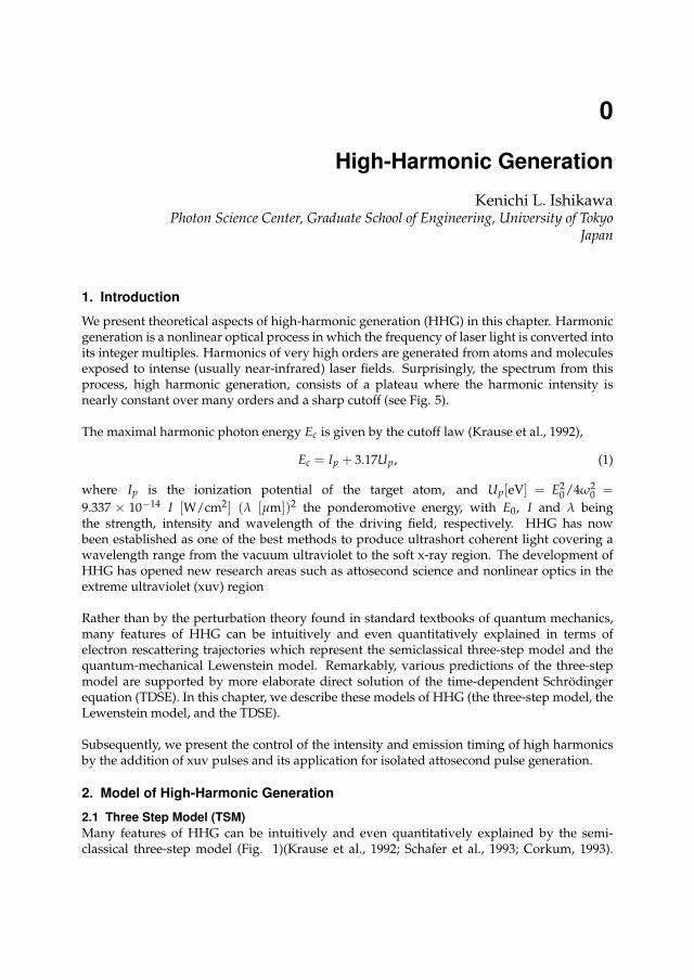
We present theoretical aspects of high-harmonic generation (HHG) in this chapter. Harmonicgeneration is a nonlinear optical process in which the frequency of laser light is converted intoits integer multiples. Harmonics of very high orders are generated from atoms and moleculesexposed to intense (usually near-infrared) laser fields. Surprisingly, the spectrum from thisprocess, high harmonic generation, consists of a plateau where the harmonic intensity isnearly constant over many orders and a sharp cutoff (see Fig. 5).

The maximal harmonic photon energy Ec is given by the cutoff law (Krause et al., 1992),

Ec = Ip + 3.17Up, (1)

where Ip is the ionization potential of the target atom, and Up[eV] = E20/4w2

0 =9.337 ⇥ 10�14 I [W/cm2] (l [µm])2 the ponderomotive energy, with E0, I and l beingthe strength, intensity and wavelength of the driving field, respectively. HHG has nowbeen established as one of the best methods to produce ultrashort coherent light covering awavelength range from the vacuum ultraviolet to the soft x-ray region. The development ofHHG has opened new research areas such as attosecond science and nonlinear optics in theextreme ultraviolet (xuv) region

Rather than by the perturbation theory found in standard textbooks of quantum mechanics,many features of HHG can be intuitively and even quantitatively explained in terms ofelectron rescattering trajectories which represent the semiclassical three-step model and thequantum-mechanical Lewenstein model. Remarkably, various predictions of the three-stepmodel are supported by more elaborate direct solution of the time-dependent Schrodingerequation (TDSE). In this chapter, we describe these models of HHG (the three-step model, theLewenstein model, and the TDSE).

Subsequently, we present the control of the intensity and emission timing of high harmonicsby the addition of xuv pulses and its application for isolated attosecond pulse generation.

2. Model of High-Harmonic Generation

2.1 Three Step Model (TSM)Many features of HHG can be intuitively and even quantitatively explained by the semi-classical three-step model (Fig. 1)(Krause et al., 1992; Schafer et al., 1993; Corkum, 1993).

According to this model, in the first step, an electron is lifted to the continuum at the nuclearposition with no kinetic energy through tunneling ionization (ionization). In the second step,the subsequent motion is governed classically by an oscillating electric field (propagation). Inthe third step, when the electron comes back to the nuclear position, occasionally, a harmonic,whose photon energy is equal to the sum of the electron kinetic energy and the ionizationpotential Ip, is emitted upon recombination. In this model, although the quantum mechanics isinherent in the ionization and recombination, the propagation is treated classically.

tunneling ionization

Ippropagation

recombinationharmonic emission

Fig. 1. Three step model of high-harmonic generation.

Let us consider that the laser electric field E(t), linearly polarized in the z direction, is givenby

E(t) = E0 cosw0t, (2)

where E0 and w0 denotes the field amplitude and frequency, respectively. If the electron isejected at t = ti, by solving the equation of motion for the electron position z(t) with the initialconditions

z(ti) = 0, (3)

z(ti) = 0, (4)

we obtain,

z(t) =E0

w20[(cosw0t � cosw0ti) + (w0t � w0ti)sinw0ti] . (5)

It is convenient to introduce the phase q ⌘ w0t. Then Equation 5 is rewritten as,

z(q) =E0

w20[(cosq � cosqi) + (q � qi)sinqi] , (6)

and we also obtain, for the kinetic energy Ekin,

Ekin(q) = 2Up (sinq � sinqi)2 . (7)

One obtains the time (phase) of recombination tr (qr) as the roots of the equation z(t) = 0(z(q) = 0). Then the energy of the photon emitted upon recombination is given by

Ekin(qr) + Ip.

Figure 2 shows Ekin(qr)/Up as a function of phase of ionization qi and recombination qr for0 < qi < p. The electron can be recombined only if 0 < qi < p/2 ; it flies away and neverreturns to the nuclear position if p/2 < qi < p. Ekin(qr) takes the maximum value 3.17Up atqi = 18� and qr = 252�. This beautifully explains why the highest harmonic energy (cutoff) isgiven by 3.17Up + Ip. It should be noted that at the time of ionization the laser field, plottedin thin solid line, is close to its maximum, for which the tunneling ionization probability ishigh. Thus, harmonic generation is efficient even near the cutoff.

3

2

1

0Ele

ctr

on

kin

etic e

ne

rgy (

in U

p)

360270180900

Phase (degrees)

-1

0

1

Fie

ld (in

E0 )

ionization recombination

short

long

short

long

field

Fig. 2. Electron kinetic energy just before recombination normalized to the ponderomotiveenergy Ekin(qr)/Up as a function of phase of ionization qi and recombination qr. The laserfield normalized to the field amplitude E(t)/E0 is also plotted in thin solid line (right axis).

For a given value of Ekin, we can view qi and qr as the solutions of the following coupledequations:

(cosqr � cosqi) + (qr � qi)sinqi = 0, (8)

(sinqr � sinqi)2 =

Ekin2Up

(9)

The path z(q) that the electron takes from q = qi to qr is called trajectory. We notice that thereare two trajectories for a given kinetic energy below 3.17Up. 18� < qi < 90�, 90� < qr < 252�for the one trajectory, and 0� < qi < 18�, 252� < qr < 360� for the other. The former is calledshort trajectory, and the latter long trajectory.

If (qi,qr) is a pair of solutions of Equations 8 and 9, (qi + mp,qr + mp) are also solu-tions, where m is an integer. If we denote z(q) associated with m as zm(q), we find thatzm(q) = (�1)mzm=0(q � mp). This implies that the harmonics are emitted each half cyclewith an alternating phase, i.e., field direction in such a way that the harmonic field Eh(t) canbe expressed in the following form:

Eh(t) = · · ·+ Fh(t + 2p/w0)� Fh(t + p/w0) + Fh(t)� Fh(t � p/w0) + Fh(t � 2p/w0)� · · · .(10)

One can show that the Fourier transform of Equation 10 takes nonzero values only at oddmultiples of w0. This observation explains why the harmonic spectrum is composed ofodd-order components.

In Fig. 3 we show an example of the harmonic field made up of the 9th, 11th, 13th, 15th, and17th harmonic components. It indeed takes the form of Equation 10. In a similar manner,high harmonics are usually emitted as a train of bursts (pulse train) repeated each half cycle ofthe fundamental laser field. The harmonic field as in this figure was experimentally observed(Nabekawa et al., 2006).

-2 -1 0 1 2

Fundamental optical cycle

harmonic field harmonic intensity fundamental field

Fig. 3. Example of the harmonic field composed of harmonic orders 9, 11, 13, 15, and 17. Thecorresponding harmonic intensity and the fundamental field are also plotted.

2.2 Lewenstein modelThe discussion of the propagation in the preceding subsection is entirely classical. Lewen-stein et al. (Lewenstein et al., 1994) developed an analytical, quantum theory of HHG, calledLewenstein model. The interaction of an atom with a laser field E(t), linearly polarized in thez direction, is described by the time-dependent Schrodinger equation (TDSE) in the lengthgauge,

i∂y(r, t)

∂t=

�1

2r2 + V(r) + zE(t)

�y(r, t), (11)

where V(r) denotes the atomic potential. In order to enable analytical discussion, they intro-duced the following widely used assumptions (strong-field approximation, SFA):

• The contribution of all the excited bound states can be neglected.• The effect of the atomic potential on the motion of the continuum electron can be ne-

glected.• The depletion of the ground state can be neglected.

Within this approximation, it can be shown (Lewenstein et al., 1994) that the time-dependentdipole moment x(t) ⌘ hy(r, t) | z | y(r, t)i is given by,

x(t) = iZ t

�•dt0Z

d3p d⇤(p + A(t)) · exp[�iS(p, t, t0)] · E(t0)d(p + A(t0)) + c.c., (12)

where p and d(p) are the canonical momentum and the dipole transition matrix element,respectively, A(t) = �R E(t)dt denotes the vector potential, and S(p, t, t0) the semiclassicalaction defined as,

S(p, t, t0) =Z t

t0dt00✓[p + A(t00)]2

2+ Ip

◆. (13)

If we approximate the ground state by that of the hydrogenic atom,

d(p) = � i8p

2(2Ip)5/4

p

p(p2 + 2Ip)3 . (14)

Alternatively, if we assume that the ground-state wave function has the form,

y(r) = (pD2)�3/4e�r2/(2D2), (15)

with D (⇠ I�1p ) being the spatial width,

d(p) = i✓

D2

p

◆3/4

D2pe�D2p2/2. (16)

In the spectral domain, Equation 12 is Fourier-transformed to, d(p) is given by,

x(wh) = iZ •

�•dtZ t

�•dt0Z

d3p d⇤(p + A(t)) · exp[iwht � iS(p, t, t0)] · E(t0)d(p + A(t0)) + c.c..

(17)Equation 12 has a physical interpretation pertinent to the three-step model: E(t0)d(p + A(t0)),exp[�iS(p, t, t0)], and d⇤(p + A(t)) correspond to ionization at time t0, propagation from t0 tot, and recombination at time t, respectively.

The evaluation of Equation 17 involves a five-dimensional integral over p, t, and t0, i.e., thesum of the contributions from all the paths of the electron that is ejected and recombined atarbitrary time and position, which reminds us of Feynman’s path-integral approach (Saliereset al., 2001). Indeed, application of the saddle-point analysis (SPA) to the integral yields asimpler expression. The stationary conditions that the first derivatives of the exponent wht �S(p, t, t0) with respect to p, t, and t0 are equal to zero lead to the saddle-point equations:

p(t � t0) +Z t

t0A(t00)dt00 = 0, (18)

[p + A(t0)]2

2= �Ip, (19)

[p + A(t)]2

2= wh � Ip, (20)

Using the solutions (ps, ts, t0s), x(wh) can be rewritten as a coherent superposition of quantumtrajectories s:

x(wh) = Âs

p

e + i2 (ts � t0s)

!3/2i2pp

detS00(t, t0)|sd⇤(ps + A(ts))

⇥exp[iwhts � iS(ps, ts, t0s)]E(t0s)d(ps + A(t0s)), (21)

where e is an infinitesimal parameter, and

detS00(t, t0)|s =✓

∂2S∂t∂t0

����s

◆2

� ∂2S∂t2

����s

∂2S∂t02

����s, (22)

∂2S∂t∂t0 =

(p + A(t))(p + A(t0))t � t0 , (23)

∂2S∂t2 = �2(wh � Ip)

t � t0 � E(t)(p + A(t)), (24)

∂2S∂t02

=2Ip

t � t0 + E(t0)(p + A(t0)), (25)

The physical meaning of Equations 18-20 becomes clearer if we note that p + A(t) is nothingbut the kinetic momentum v(t). Equation 18, rewritten as

R tt0 v(t00)dt00 = 0, indicates that

the electron appears in the continuum and is recombined at the same position (nuclearposition). Equation 20, rewritten together with Equation 19 as v(t)2/2 � v(t0)2/2 = wh,means the energy conservation. The interpretation of Equation 18 is more complicated, sinceits right-hand side is negative, which implies that the solutions of the saddle-point equationsare complex in general. The imaginary part of t0 is usually interpreted as tunneling time(Lewenstein et al., 1994).

Let us consider again that the laser electric field is given by Equation 2 and introduce q = w0tand k = pw0/E0. Then Equations 18-20 read as,

k = � cosq � cosq0q � q0 , (26)

(k � sinq0)2 = � Ip

2Up= �g2, (27)

(k � sinq)2 =wh � Ip

2Up, (28)

where g is called the Keldysh parameter. If we replace Ip and wh � Ip in these equations byzero and Ekin, respectively, we recover Equations 8 and 9 for the three-step model. Figure 4displays the solutions (q,q0) of these equations as a function of harmonic order. To make ourdiscussion concrete, we consider harmonics from an Ar atom (Ip = 15.7596eV) irradiated by alaser with a wavelength of 800 nm and an intensity of 1.6 ⇥ 1014 W/cm2. The imaginary partof q0 (Fig. 4 (b)) corresponds to the tunneling time, as already mentioned. On the other hand,the imaginary part of q is much smaller; that for the long trajectory, in particular, is nearlyvanishing below the cutoff (⇡ 32nd order), which implies little contribution of tunneling tothe recombination process. In Fig. 4 (a) are also plotted in thin dashed lines the trajectoriesfrom Fig. 2, obtained with the three-step model. We immediately notice that the Lewensteinmodel predicts a cutoff energy Ec,

Ec = 3.17Up + gIp (g ⇡ 1.3), (29)

slightly higher than the three-step model (Lewenstein et al., 1994). This can be understoodqualitatively by the fact that there is a finite distance between the nucleus and the tunnel exit(Fig. 1); the electron which has returned to the position of the tunnel exit is further accelerated

till it reaches the nuclear position. Except for the difference in Ec, the trajectories from the TSMand the SPA (real part) are close to each other, though we see some discrepancy in the ioniza-tion time of the short trajectory. This suggests that the semi-classical three-step model is usefulto predict and interpret the temporal structure of harmonic pulses, primarily determined bythe recombination time, as we will see later.

1.0

0.5

0.0

-0.5Imagin

ary

part

(ra

d)

3530252015

Harmonic order

(b)

Recombination

Short trajectory

Short trajectory

Long trajectory

Long trajectory

Ionization

6

4

2

0

Real part

(ra

d)

3530252015

(a)

Long trajectory

Short trajectory

Long trajectory

Short trajectory Ionization

Recombination

Fig. 4. (a) Real and (b) imaginary parts (radian) of the solutions q (for recombination) andq0 (for ionization) of Equations 26-28 as a function of harmonic order wh/w0. The value ofIp = 15.7596eV is for Ar. The wavelength and intensity of the driving laser are 800 nm and1.6 ⇥ 1014 W/cm2. Thin dashed lines in panel (a) correspond to the three-step model.

2.3 Gaussian modelIn the Gaussian model, we assume that the ground-state wave function has a form given byEquation 15. An appealing point of this model is that the dipole transition matrix elementalso takes a Gaussian form (Equation 16) and that one can evaluate the integral with respectto momentum in Equation 12 analytically, without explicitly invoking the notion of quantumpaths. Thus, we obtain the formula for the dipole moment x(t) as,

x(t) = i D�7Z t

�•(2C(t, t0))3/2E(t0)

⇥ {A(t)A(t0) + C(t, t0)[1 � D(t, t0)(A(t) + A(t0))] + C2(t, t0)D2(t, t0)}

⇥ exp✓�i[Ip(t � t0) + B(t, t0)]� [A2(t) + A2(t0)]D2 � C(t, t0)D2(t, t0)

2

◆dt0, (30)

where B(t, t0), C(t, t0), and D(t, t0) are given by,

B(t, t0) =12

Z t

t0dt00A2(t00) , (31)

C(t, t0) =1

2D2 + i(t � t0), (32)

D(t, t0) = [A(t) + A(t0)]D2 + iZ t

t0dt00A(t00) . (33)

The Gaussian model is also useful when one wants to account for the effect of the initial spatialwidth of the wave function within the framework of the Lewenstein model (Ishikawa et al.,2009b).

2.4 Direct simulation of the time-dependent Schrodinger equation (TDSE)The most straightforward way to investigate HHG based on the time-dependent Schrodingerequation 11 is to solve it numerically. Such an idea might sound prohibitive at first, the TDSEsimulations are indeed frequently used, with the rapid progress in computer technology. Thisapproach provides us with exact numerical solutions, which are powerful especially when weface new phenomena for which we do not know a priori what kind of approximation is valid.We can also analyze the effects of the atomic Coulomb potential, which is not accounted forby the models in the preceding subsections. Here we briefly present the method developedby Kulander et al. (Kulander et al., 1992) for an atom initially in an s state. There are alsoother methods, such as the pseudo-spectral method (Tong & Chu, 1997) and those using thevelocity gauge (Muller, 1999; Bauer & Koval, 2006).

Since we assume linear polarization in the z direction, the angular momentum selection ruletells us that the magnetic angular momentum remains m = 0. Then we can expand the wavefunction y(r, t) in spherical harmonics with m = 0,

y(r, t) = Âl

Rl(r, t)Y0l (q,f). (34)

At this stage, the problem of three dimensions in space physically has been reduced to twodimensions. By discretizing the radial wave function Rl(r, t) as gj

l = rjRl(rj, t) with rj = (j �12 )Dr, where Dr is the grid spacing, we can derive the following equations for the temporalevolution (Kulander et al., 1992):

i∂

∂tgj

l = � cjgj+1l � 2djg

jl + cj�1gj�1

l2(Dr)2 +

l(l + 1)

2r2j

+ V(rj)

!gj

l (35)

+ rjE(t)⇣

al gjl+1 + al�1gj

l�1

⌘

= (H0g)jl + (HI g)j

l , (36)

where the coefficients are given by,

cj =j2

j2 � 1/4, dj =

j2 � j + 1/2j2 � j + 1/4

, al =l + 1p

(2l + 1)(2l + 3). (37)

Here, in order to account for the boundary condition at the origin properly, the Euler-Lagrangeequations with a Lagrange-type functional (Kulander et al., 1992; Koonin et al., 1977),

L = hy | i∂/∂t � (H0 + HI(t)) | yi, (38)

has been discretized, instead of Equation 11 itself. cj and dj tend to unity for a large valueof j, i.e., a large distance from the nucleus, with which the first term of the right-handside of Equation 35 becomes an ordinary finite-difference expression. The operator H0corresponds to the atomic Hamiltonian and is diagonal in l, while HI corresponds to theinteraction Hamiltonian and couples the angular momentum l to the neighboring values l ± 1.

Equations 35 and 36 can be integrated with respect to t by the alternating direction implicit(Peaceman-Rachford) scheme,

gjl(t + Dt) = [I + iH0t/2]�1[I + iHI t/2]�1[I � iHI t/2][I � iH0t/2], (39)

with Dt being the time step. This algorithm is accurate to the order of O(Dt3), and approxi-mately unitary. One can reduce the difference between the discretized and analytical wavefunction, by scaling the Coulomb potential by a few percent at the first grid point (Krauseet al., 1992). We can obtain the harmonic spectrum by Fourier-transforming the dipoleacceleration x(t) = �∂2

t hz(t)i, which in turn we calculate, employing the Ehrenfest theoremthrough the relation x(t) = hy(r, t) | cosq/r2 � E(t) | y(r, t)i(Tong & Chu, 1997), where thesecond term can be dropped as it does not contribute to the HHG spectrum.

V(r) is the bare Coulomb potential for a hydrogenic atom. Otherwise, we can employ a modelpotential (Muller & Kooiman, 1998) within the single-active electron approximation (SAE),

V(r) = �[1 + Ae�r + (Z � 1 � A)e�Br]/r, (40)

where Z denotes the atomic number. Parameters A, and B are chosen in such a way thatthey faithfully reproduce the eigenenergies of the ground and the first excited states. One canaccount for nonzero azimuthal quantum numbers by replacing al by (Kulander et al., 1992),

aml =

s(l + 1)2 � m2

(2l + 1)(2l + 3). (41)

In Fig. 5 we show an example of the calculated harmonic spectrum for a hydrogen atomirradiated by a Ti:Sapphire laser pulse with a wavelength of 800 nm (hw0 = 1.55eV) and apeak intensity of 1.6 ⇥ 1014 W/cm2. The laser field E(t) has a form of E(t) = f (t)sinw0t,where the field envelope f (t) corresponds to a 8-cycle flat-top sine pulse with a half-cycleturn-on and turn-off. We can see that the spectrum has peaks at odd harmonic orders, as isexperimentally observed, and the cutoff energy predicted by the cutoff law.

3. High-harmonic generation by an ultrashort laser pulse

Whereas in the previous section we considered the situation in which the laser has a constantintensity in time, virtually all the HHG experiments are performed with an ultrashort(a few to a few tens of fs) pulse. The state-of-the-art laser technology is approaching asingle-cycle limit. The models in the preceding section can be applied to such situations

10-8

10-7

10-6

10-5

10-4

10-3

10-2

10-1

100

101

102

Harm

onic

inte

nsity (

arb

. unit)

50403020100

Harmonic order

Fig. 5. HHG spectrum from a hydrogen atom, calculated with the Peaceman-Rachfordmethod. See text for the laser parameters.

without modification.

For completeness, the equations for the recombination time t and ionization time t0 in thethree-step model is obtained by replacing Ip in the right-hand side of Equation 19 by zero asfollows:

� A(t0)(t � t0) +Z t

t0A(t00)dt00 = 0, (42)

[A(t)� A(t0)]2

2= wh � Ip. (43)

The canonical momentum is given by p = �A(t0).

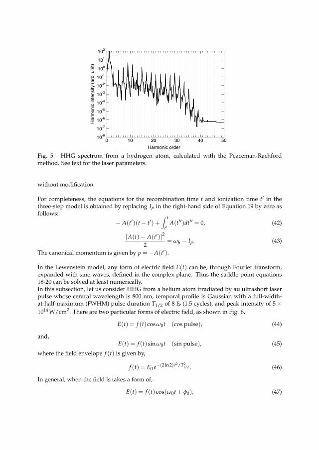
In the Lewenstein model, any form of electric field E(t) can be, through Fourier transform,expanded with sine waves, defined in the complex plane. Thus the saddle-point equations18-20 can be solved at least numerically.In this subsection, let us consider HHG from a helium atom irradiated by au ultrashort laserpulse whose central wavelength is 800 nm, temporal profile is Gaussian with a full-width-at-half-maximum (FWHM) pulse duration T1/2 of 8 fs (1.5 cycles), and peak intensity of 5 ⇥1014 W/cm2. There are two particular forms of electric field, as shown in Fig. 6,

E(t) = f (t)cosw0t (cos pulse), (44)

and,E(t) = f (t)sinw0t (sin pulse), (45)

where the field envelope f (t) is given by,

f (t) = E0 e�(2ln2) t2/T21/2 . (46)

In general, when the field is takes a form of,

E(t) = f (t)cos(w0t + f0), (47)

-0.15

-0.10

-0.05

0.00

0.05

0.10

0.15

Fie

ld (

a.u

.)

20100-10-20

Time (fs)

cos pulse sin pulse

Fig. 6. Electric fields of cos and sin pulses.

f0 is call carrier-envelope phase (CEP). The CEP is zero and �p/2 for cos and sin pulses, respec-tively.

400

300

200

100Ha

rmo

nic

en

erg

y (

eV

)

86420-2-4-6

Time (fs)

-0.1

0.0

0.1 Fie

ld (a

.u.)

(a)

10-12

10-11

10-10

10-9

10-8

10-7

10-6

10-5

10-4

10-3

10-2

10-1

Ha

rmo

nic

in

ten

sity (

arb

. u

nit)

5004003002001000

Harmonic energy (eV)

(b)

Fig. 7. (a) Real part of the recombination (red) and ionization times (blue) calculated fromthe saddle-point equations for the cos pulse. Each trajectory pair is labeled from A to E. Theblack dashed line is the recombination time from the three-step model. The electric field isalso shown in black solid line. (b) Harmonic spectrum calculated with direct simulation of theTDSE.

3.1 Cos pulseFigure 7 (a) displays the real part of the recombination (t) and ionization (t0) times calculatedwith the saddle-point equations for the 1.5-cycle cos pulse. The recombination time fromthe three-step model, also shown in this figure, is close to the real part of the saddle-pointsolutions. By comparing this figure with the harmonic spectrum calculated with directsimulation of the TDSE (Fig. 7 (b)), we realize that the steps around 400 and 300 eV in thespectrum correspond to the cutoff of trajectory pairs C and D. Why do not a step (cutoff) for

1.5

1.0

0.5

0.0

x1

0-8

86420-2-4-6

Time (fs)

(c) 225-275 eV 275-325 eV 325-375 eV 375-425 eV

C

D

sh

ort s

ho

rt

lon

g

lon

g

1.5

1.0

0.5

0.0

x1

0-8

86420-2-4-6

(b) > 200 eV C D

1.0

0.8

0.6

0.4

0.2

0.0x10

-8

86420-2-4-6

(a) > 300 eV C

Sq

ua

red

dip

ole

acce

lera

tio

n (

a.u

.)

Fig. 8. Temporal profile of the TDSE-calculated squared dipole acceleration (SDA), propor-tional to the harmonic pulse intensity generated by the cos pulse, (a) at hwh > 200 eV, (b) athwh > 300 eV, (c) for different energy ranges indicated in the panel. Labels C and D indicatecorresponding trajectory pairs in Fig. 7 (a). Labels “short” and “long” indicate short and longtrajectories, respectively.

pair B appear? This is related to the field strength at time of ionization, indicated with verticalarrows in Fig. 7 (a). That for pair B (⇠ -5 fs) is smaller than those of pairs C (⇠ -2.5 fs) and D(⇠ 0 fs). Since the tunneling ionization rate (the first step of the three-step model) dependsexponentially on intensity, the contribution from pair B is hidden by those from pairs C andD. It is noteworthy that the trajectory pair C for the cutoff energy (⇠ 400 eV) is ionized notat the pulse peak but half cycle before it. Then the electron is accelerated efficiently by thesubsequent pulse peak.

From the above consideration, and also remembering that harmonic emission occurs uponrecombination, we can speculate the following:

• The harmonics above 200 eV consists of a train of two pulses at t ⇡ 1 (C) and 3.5 fs (D).

• By extracting the spectral component above 300 eV, one obtains an isolated attosecondpulse at t ⇡ 1 fs (C).

• The emission from the short (long) trajectories are positively (negatively) chirped, i.e.,the higher the harmonic order, the later (the earlier) the emission time. The chirp leadsto temporal broadening of the pulse.

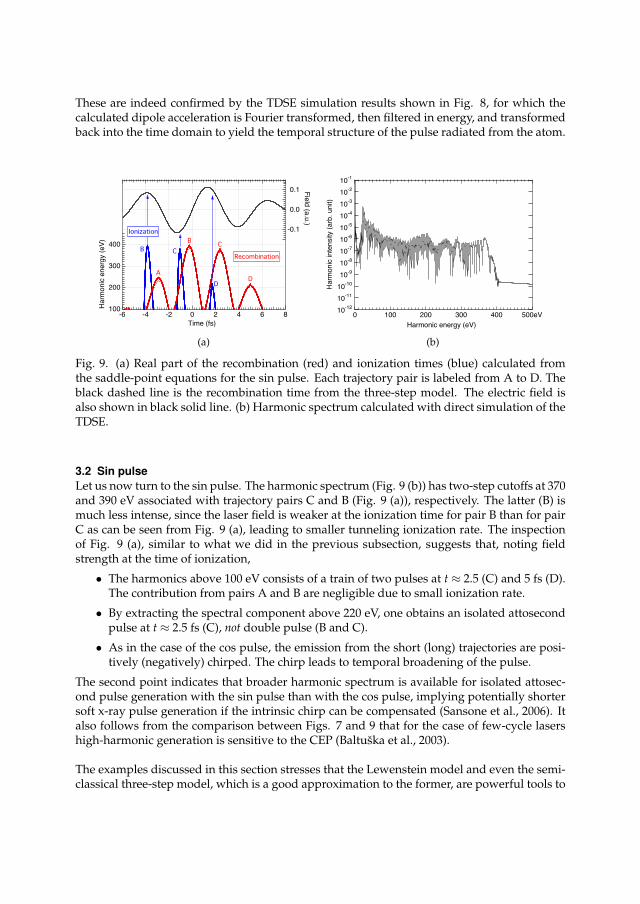
These are indeed confirmed by the TDSE simulation results shown in Fig. 8, for which thecalculated dipole acceleration is Fourier transformed, then filtered in energy, and transformedback into the time domain to yield the temporal structure of the pulse radiated from the atom.

400

300

200

100Ha

rmo

nic

en

erg

y (

eV

)

86420-2-4-6

Time (fs)

-0.1

0.0

0.1 Fie

ld (a

.u.)

(a)

10-12

10-11

10-10

10-9

10-8

10-7

10-6

10-5

10-4

10-3

10-2

10-1

Ha

rmo

nic

in

ten

sity (

arb

. u

nit)

500eV4003002001000

Harmonic energy (eV)

(b)

Fig. 9. (a) Real part of the recombination (red) and ionization times (blue) calculated fromthe saddle-point equations for the sin pulse. Each trajectory pair is labeled from A to D. Theblack dashed line is the recombination time from the three-step model. The electric field isalso shown in black solid line. (b) Harmonic spectrum calculated with direct simulation of theTDSE.

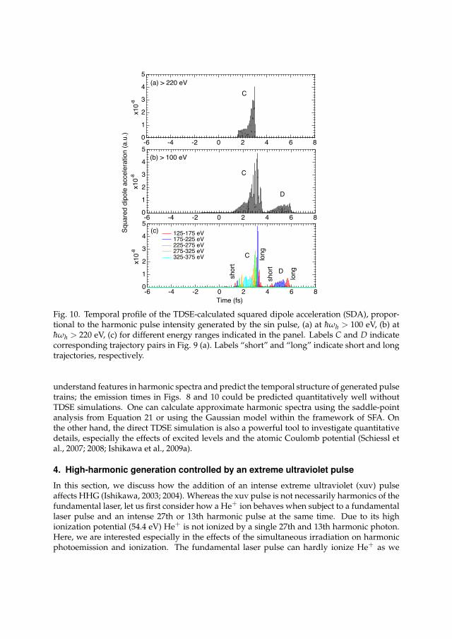
3.2 Sin pulseLet us now turn to the sin pulse. The harmonic spectrum (Fig. 9 (b)) has two-step cutoffs at 370and 390 eV associated with trajectory pairs C and B (Fig. 9 (a)), respectively. The latter (B) ismuch less intense, since the laser field is weaker at the ionization time for pair B than for pairC as can be seen from Fig. 9 (a), leading to smaller tunneling ionization rate. The inspectionof Fig. 9 (a), similar to what we did in the previous subsection, suggests that, noting fieldstrength at the time of ionization,

• The harmonics above 100 eV consists of a train of two pulses at t ⇡ 2.5 (C) and 5 fs (D).The contribution from pairs A and B are negligible due to small ionization rate.

• By extracting the spectral component above 220 eV, one obtains an isolated attosecondpulse at t ⇡ 2.5 fs (C), not double pulse (B and C).

• As in the case of the cos pulse, the emission from the short (long) trajectories are posi-tively (negatively) chirped. The chirp leads to temporal broadening of the pulse.

The second point indicates that broader harmonic spectrum is available for isolated attosec-ond pulse generation with the sin pulse than with the cos pulse, implying potentially shortersoft x-ray pulse generation if the intrinsic chirp can be compensated (Sansone et al., 2006). Italso follows from the comparison between Figs. 7 and 9 that for the case of few-cycle lasershigh-harmonic generation is sensitive to the CEP (Baltuska et al., 2003).

The examples discussed in this section stresses that the Lewenstein model and even the semi-classical three-step model, which is a good approximation to the former, are powerful tools to

5

4

3

2

1

0x1

0-8

86420-2-4-6

(a) > 220 eV

C

5

4

3

2

1

0

x1

0-8

86420-2-4-6

Time (fs)

125-175 eV 175-225 eV 225-275 eV 275-325 eV 325-375 eV

(c)

C

D

sh

ort

sh

ort

lo

ng

lon

g

5

4

3

2

1

0

x1

0-8

86420-2-4-6

(b) > 100 eV

C

D

Sq

ua

red

dip

ole

acce

lera

tio

n (

a.u

.)

Fig. 10. Temporal profile of the TDSE-calculated squared dipole acceleration (SDA), propor-tional to the harmonic pulse intensity generated by the sin pulse, (a) at hwh > 100 eV, (b) athwh > 220 eV, (c) for different energy ranges indicated in the panel. Labels C and D indicatecorresponding trajectory pairs in Fig. 9 (a). Labels “short” and “long” indicate short and longtrajectories, respectively.

understand features in harmonic spectra and predict the temporal structure of generated pulsetrains; the emission times in Figs. 8 and 10 could be predicted quantitatively well withoutTDSE simulations. One can calculate approximate harmonic spectra using the saddle-pointanalysis from Equation 21 or using the Gaussian model within the framework of SFA. Onthe other hand, the direct TDSE simulation is also a powerful tool to investigate quantitativedetails, especially the effects of excited levels and the atomic Coulomb potential (Schiessl etal., 2007; 2008; Ishikawa et al., 2009a).

4. High-harmonic generation controlled by an extreme ultraviolet pulse

In this section, we discuss how the addition of an intense extreme ultraviolet (xuv) pulseaffects HHG (Ishikawa, 2003; 2004). Whereas the xuv pulse is not necessarily harmonics of thefundamental laser, let us first consider how a He+ ion behaves when subject to a fundamentallaser pulse and an intense 27th or 13th harmonic pulse at the same time. Due to its highionization potential (54.4 eV) He+ is not ionized by a single 27th and 13th harmonic photon.Here, we are interested especially in the effects of the simultaneous irradiation on harmonicphotoemission and ionization. The fundamental laser pulse can hardly ionize He+ as we

will see later. Although thanks to high ionization potential the harmonic spectrum from thision would have higher cut-off energy than in the case of commonly used rare-gas atoms, theconversion efficiency is extremely low due to the small ionization probability. It is expected,however, that the addition of a Ti:Sapphire 27th or 13th harmonic facilitates ionization andphotoemission, either through two-color frequency mixing or by assisting transition to the2p or 2s levels. The direct numerical solution of the time-dependent Schrodinger equationshows in fact that the combination of fundamental laser and its 27th or 13th harmonic pulsesdramatically enhance both high-order harmonic generation and ionization by many orders ofmagnitude.

To study the interaction of a He+ ion with a combined laser and xuv pulse, we solve thetime-dependent Schrodinger equation in the length gauge,

i∂F(r, t)

∂t=

�1

2r2 � 2

r� zE(t)

�F(r, t), (48)

where E(t) is the electric field of the pulse. Here we have assumed that the field is linearlypolarized in the z-direction. To prevent reflection of the wave function from the grid boundary,after each time step the wave function is multiplied by a cos1/8 mask function (Krause et al.,1992) that varies from 1 to 0 over a width of 2/9 of the maximum radius at the outer radialboundary. The ionization yield is evaluated as the decrease of the norm of the wave functionon the grid. The electric field E(t) is assumed to be given by,

E(t) = FF(t)sin(wt) + FH(t)sin(nwt + f), (49)

with FF(t) and FH(t) being the pulse envelope of the fundamental and harmonic pulse, re-spectively, chosen to be Gaussian with a duration (full width at half maximum) of 10 fs, w theangular frequency of the fundamental pulse, n the harmonic order, and f the relative phase.The fundamental wavelength is 800 nm unless otherwise stated. Since we have found that theresults are not sensitive to f, we set f = 0 hereafter.

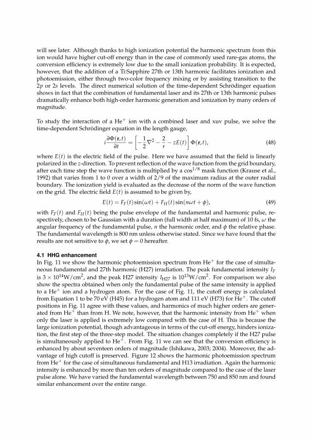
4.1 HHG enhancementIn Fig. 11 we show the harmonic photoemission spectrum from He+ for the case of simulta-neous fundamental and 27th harmonic (H27) irradiation. The peak fundamental intensity IFis 3 ⇥ 1014W/cm2, and the peak H27 intensity IH27 is 1013W/cm2. For comparison we alsoshow the spectra obtained when only the fundamental pulse of the same intensity is appliedto a He+ ion and a hydrogen atom. For the case of Fig. 11, the cutoff energy is calculatedfrom Equation 1 to be 70 eV (H45) for a hydrogen atom and 111 eV (H73) for He+. The cutoffpositions in Fig. 11 agree with these values, and harmonics of much higher orders are gener-ated from He+ than from H. We note, however, that the harmonic intensity from He+ whenonly the laser is applied is extremely low compared with the case of H. This is because thelarge ionization potential, though advantageous in terms of the cut-off energy, hinders ioniza-tion, the first step of the three-step model. The situation changes completely if the H27 pulseis simultaneously applied to He+. From Fig. 11 we can see that the conversion efficiency isenhanced by about seventeen orders of magnitude (Ishikawa, 2003; 2004). Moreover, the ad-vantage of high cutoff is preserved. Figure 12 shows the harmonic photoemission spectrumfrom He+ for the case of simultaneous fundamental and H13 irradiation. Again the harmonicintensity is enhanced by more than ten orders of magnitude compared to the case of the laserpulse alone. We have varied the fundamental wavelength between 750 and 850 nm and foundsimilar enhancement over the entire range.

10-21

10

-18

10-15

10

-12

10-9

10-6

10-3

100

103

106

Inte

nsity (

arb

.unit)

100806040200Harmonic order (fundamental wavelength = 800nm)

Hydrogen atom

He+

Laser alone (3x1014

W/cm2)

He+

Laser (3x1014

W/cm2) + H27 (10

13 W/cm

2)

Fig. 11. Upper solid curve: harmonic spectrum from He+ exposed to a Gaussian combinedfundamental and its 27th harmonic pulse with a duration (FWHM) of 10 fs, the former with apeak intensity of 3 ⇥ 1014 W/cm2 and the latter 1013 W/cm2. The fundamental wavelength is800 nm. Lower solid and dotted curves: harmonic spectrum from He+ and a hydrogen atom,respectively, exposed to the fundamental pulse alone. Nearly straight lines beyond the cut-offenergy are due to numerical noise.

10-13

10

-11

10-9

10-7

10-5

10-3

10-1

101

103

105

107

Inte

nsity (

arb

.unit)

100806040200Harmonic order (fundamental wavelength = 800 nm)

Laser (3x1014

W/cm2)

+ H13 (1014

W/cm2)

Laser (3x1014

W/cm2)

+ H13 (1012

W/cm2)

Fig. 12. Harmonic spectrum from He+ exposed to a Gaussian combined fundamental andits 13th harmonic pulse with a duration (FWHM) of 10 fs, the former with a peak intensity of3⇥ 1014 W/cm2, and the latter 1014 W/cm2 (upper curve) and 1012 W/cm2 (lower curve). Thefundamental wavelength is 800 nm. Note that the horizontal axis is of the same scale as in Fig.11.

Table 1. The He2+ yield for various combinations of a Gaussian fundamental and its 27th or13th harmonic pulses with a duration (FWHM) of 10 fs and a peak intensity listed in the table.lF = 800 nm.

IF (W/cm2) IH27 (W/cm2) IH13 (W/cm2) He2+ yield3 ⇥ 1014 � � 2.29 ⇥ 10�15

� 1013 � 4.79 ⇥ 10�6

3 ⇥ 1014 1013 � 0.173� � 1014 1.25 ⇥ 10�4

3 ⇥ 1014 � 1014 2.04 ⇥ 10�4

4.2 Enhancement mechanismThe effects found in Figs. 11 and 12 can be qualitatively understood as follows. The H27photon energy (41.85 eV) is close to the 1s-2p transition energy of 40.8 eV, and the H13 photon(20.15 eV) is nearly two-photon resonant with the 1s-2s transition. Moreover, the 2p and2s levels are broadened due to laser-induced dynamic Stark effect. As a consequence, theH27 and H13 promote transition to a virtual state near these levels. Depending on the laserwavelength, resonant excitation of 2s or 2p levels, in which fundamental photons may beinvolved in addition to harmonic photons, also takes place. In fact, the 2s level is excitedthrough two-color two-photon transition for the case of Fig. 11 at lF = 800 nm, as we will seebelow in Fig. 15, and about 8% of electron population is left in the 2s level after the pulse.Since this level lies only 13.6 eV below the ionization threshold, the electron can now belifted to the continuum by the fundamental laser pulse much more easily and subsequentlyemit a harmonic photon upon recombination. Thus the HHG efficiency is largely increased.We have found that the harmonic spectrum from the superposition of the 1s (92%) and 2s(8%) states subject to the laser pulse alone is strikingly similar to the one in Fig. 11. Hencethe effect may also be interpreted as harmonic generation from a coherent superpositionof states (Watson et al., 1996). On the other hand, at a different fundamental wavelength,e.g., at lF = 785 nm, there is practically no real excitation. Nevertheless the photoemissionenhancement (not shown) is still dramatic. This indicates that fine tuning of the xuv pulse tothe resonance with an excited state is not necessary for the HHG enhancement. In this case,the H27 pulse promotes transition to a virtual state near the 2p level. Again, the electroncan easily be lifted from this state to the continuum by the fundamental pulse, and the HHGefficiency is largely augmented. This may also be viewed as two-color frequency mixingenhanced by the presence of a near-resonant intermediate level. In general, both mechanismsof harmonic generation from a coherent superposition of states and two-color frequencymixing coexist, and their relative importance depends on fundamental wavelength. A similardiscussion applies to the case of the H13 addition. The comparison of the two curves in Fig.12 reveals that the harmonic spectrum is proportional to I2

H13, where IH13 denotes the H13peak intensity. We have also confirmed that the photoemission intensity is proportional toIH27 for the case of H27. These observations are compatible with the discussion above.

4.3 Ionization enhancementLet us now examine ionization probability. Table 1 summarizes the He2+ yield for each caseof the fundamental pulse alone, the harmonic pulse alone, and the combined pulse. As canbe expected from the discussion in the preceding paragraph, the ionization probability by

10-10

10-9

10-8

10-7

10-6

10-5

10-4

10-3

10-2

10-1

100

He

2+ y

ield

1011

2 3 4 5 6

1012

2 3 4 5 6

1013

2 3 4 5 6

1014

H27 or H13 intensity (W/cm2)

H27

H13

Fig. 13. The He2+ yield as a function of peak intensity of the 27th (upper curve) and 13th(lower curve) harmonic pulse when He+ is exposed to a Gaussian combined fundamentaland its 27th harmonic pulse with a duration (FWHM) of 10 fs. The wavelength lF and thepeak intensity IF of the fundamental pulse are 800 nm and 3 ⇥ 1014 W/cm2, respectively.

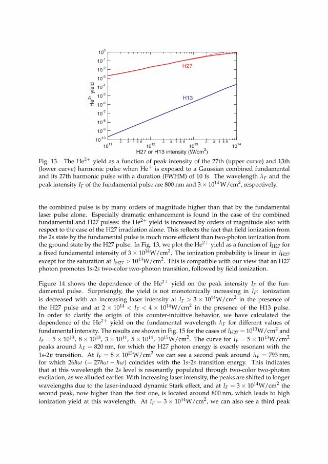
the combined pulse is by many orders of magnitude higher than that by the fundamentallaser pulse alone. Especially dramatic enhancement is found in the case of the combinedfundamental and H27 pulses: the He2+ yield is increased by orders of magnitude also withrespect to the case of the H27 irradiation alone. This reflects the fact that field ionization fromthe 2s state by the fundamental pulse is much more efficient than two-photon ionization fromthe ground state by the H27 pulse. In Fig. 13, we plot the He2+ yield as a function of IH27 fora fixed fundamental intensity of 3 ⇥ 1014W/cm2. The ionization probability is linear in IH27except for the saturation at IH27 > 1013W/cm2. This is compatible with our view that an H27photon promotes 1s-2s two-color two-photon transition, followed by field ionization.

Figure 14 shows the dependence of the He2+ yield on the peak intensity IF of the fun-damental pulse. Surprisingly, the yield is not monotonically increasing in IF: ionizationis decreased with an increasing laser intensity at IF > 3 ⇥ 1014W/cm2 in the presence ofthe H27 pulse and at 2 ⇥ 1014 < IF < 4 ⇥ 1014W/cm2 in the presence of the H13 pulse.In order to clarify the origin of this counter-intuitive behavior, we have calculated thedependence of the He2+ yield on the fundamental wavelength lF for different values offundamental intensity. The results are shown in Fig. 15 for the cases of IH27 = 1013W/cm2 andIF = 5 ⇥ 1013, 8 ⇥ 1013, 3 ⇥ 1014, 5 ⇥ 1014, 1015W/cm2. The curve for IF = 5 ⇥ 1013W/cm2

peaks around lF = 820 nm, for which the H27 photon energy is exactly resonant with the1s-2p transition. At IF = 8 ⇥ 1013W/cm2 we can see a second peak around lF = 793 nm,for which 26hw (= 27hw � hw) coincides with the 1s-2s transition energy. This indicatesthat at this wavelength the 2s level is resonantly populated through two-color two-photonexcitation, as we alluded earlier. With increasing laser intensity, the peaks are shifted to longerwavelengths due to the laser-induced dynamic Stark effect, and at IF = 3 ⇥ 1014W/cm2 thesecond peak, now higher than the first one, is located around 800 nm, which leads to highionization yield at this wavelength. At IF = 3 ⇥ 1014W/cm2, we can also see a third peak

10-10

10-9

10-8

10-7

10-6

10-5

10-4

10-3

10-2

10-1

100

He

2+ y

ield

1011

1012

1013

1014

1015

Laser intensity (W/cm2)

H27 (1013

W/cm2)

H13 (1012

W/cm2)

H27 (1012

W/cm2)

H13 (1013

W/cm2)

Fig. 14. The He2+ yield as a function of peak intensity IF of the fundamental laser pulse whenHe+ is exposed to a Gaussian combined fundamental and its 27th or 13th harmonic pulse witha duration (FWHM) of 10 fs. The fundamental wavelength lF is 800 nm. The peak intensityof each harmonic pulse is indicated in the figure along with its order.

0.20

0.15

0.10

0.05

0.00

He

2+ y

ield

840820800780760

Fundamental wavelength (nm)

Fundamental intensity

1015

W/cm2

5x1014

W/cm2

3x1014

W/cm2

8x1013

W/cm2

5x1013

W/cm2

Fig. 15. The He2+ yield as a function of fundamental wavelength when He+ is exposed to aGaussian combined fundamental and its 27th harmonic pulse with a duration (FWHM) of 10fs. The peak intensity IH27 of the 27th harmonic pulse is fixed at 1013 W/cm2, and we plot theresults for five different values of fundamental peak intensity IF indicated in the figure. Notethat the wavelength of the 27th harmonic varies with that of the fundamental pulse.

10-14

10

-12

10-10

10

-8

10-6

10-4

10-2

100

102

Harm

onic

spectr

um

(arb

. units)

200eV150100500

Photon enegy (eV)

Driving wavelength = 1600 nm

Fund. (1.6x1014

W/cm2) & XUV (YI=0.31%)

Fund. only (1.6x1014

W/cm2) (YI=1.7x10

-5%)

Fig. 16. Upper curve: harmonic spectrum from He exposed to a 35 fs Gaussian combineddriving and XUV pulse (hwX = 17.05eV), the former (l = 1600 nm) with a peak intensity of1.6 ⇥ 1014 W/cm2 and the latter 2.3 ⇥ 1011 W/cm2. Middle curve: harmonic spectra for thecases of the driving pulse alone, with an intensity of 1.6 ⇥ 1014 W/cm2.

around lF = 770 nm corresponding to two-color 2p excitation involving one H27 and twofundamental photons. The dynamic Stark effect induces not only the peak shift but alsothe peak broadening, which results in the decrease of peak heights at higher fundamentalintensity, leading to the decrease of the ionization yield at IF > 3 ⇥ 1014W/cm2 in Fig. 14.Thus, the role of the fundamental laser pulse is three-fold: to lift the electron in an excited(real or virtual) level to the continuum through optical-field ionization, to assist 1s-2s, 2ptransitions through two-color excitation, and to induce dynamic Stark shift and broadening.The interplay of these three leads to a complicated behavior seen in Fig. 14.

4.4 RemarksThe mechanism of the HHG enhancement discussed above is that the xuv addition increasesthe field ionization rate by promoting transition to (real or virtual) excited states, from whichionization is much easier than from the ground state. Hence, the enhancement is effectiveonly when the ionization rate by the fundamental pulse alone is not high enough. If HHG is alreadyoptimized by a sufficiently intense laser pulse, the xuv addition does not increase the HHGyield significantly.

Although the cases involving resonant transitions are highlighted above, the resonancewith an excited state is not necessary for the enhancement. Figure 16 shows the harmonicspectra from He for l = 1600nm with and without the XUV field (hwX = 17.05eV). For thecase of the driving laser alone with a peak intensity I of 1.6 ⇥ 1014 W/cm2 (blue curve), theionization yield YI is very low (1.7 ⇥ 10�5%). The addition of the xuv pulse with an intensityof 2.3 ⇥ 1011 W/cm2 increases YI to 0.31% and enhances the harmonic yield accordingly (redcurve). In this case, the xuv photon energy is not resonance with transition to excited states.Nevertheless, the HHG yield is enhanced by orders of magnitude. The dramatic enhancement

effect has been experimentally demonstrated by the use of mixed gases (Takahashi et al.,2007); also in this experiment, the booster xuv pulse (harmonics from Xe) was non-resonantwith the target atom (He).

4.5 Single attosecond pulse generation using the enhancement effectThe progress in the high-harmonic generation (HHG) technique has raised significant interestin the generation of attosecond pulses. As we have seen in Subsec. 2.1, the photoemissionprocess is repeated every half-cycle of the laser optical field and produces an attosecondpulse train (Fig. 1). On the other hand, a single attosecond pulse (SAP), in particular, iscritical for the study of the electron dynamics inside atoms(Krausz & Ivanov, 2009). If thedriving laser pulse is sufficiently short that the effective HHG takes place only within onehalf-cycle, the cut-off region of the spectrum may become a continuum, corresponding to asingle recollision (Figs. 8 and 10). The first SAPs (Baltuska et al., 2003) were obtained on thisbasis. Isolated attosecond pulses have also been realized by other methods such as ionizationshutter (Sekikawa et al., 2004), polarization gate (Corkum et al., 1994), and two-color scheme(Pfeifer et al., 2006).

The enhancement effect discussed in the preceding subsections provides a means to controlHHG and new physical insights (Schafer et al., 2004; Ishikawa et al., 2009b). As an example,in this subsection, we present an alternative method of SAP generation multi-cycle laserpulses, called attosecond enhancement gate for isolated pulse generation (AEGIS) (Ishikawa etal., 2007). Let us first describe AEGIS qualitatively (Figs. 17(a) and 18(a)). The underlyingmechanism of the HHG enhancement by the addition of xuv pulses is that the seed pulseinduces transition to real or virtual excited levels, facilitating optical-field ionization, the firststep of the three-step model. When the seed is composed of a train of attosecond pulses,this can be viewed as repeated attosecond enhancement gates. Let us consider that thefundamental pulse generating the seed harmonic pulse, referred to as the seed fundamentalpulse hereafter, and the driving laser pulse which will be combined with the seed pulse havedifferent wavelengths. For example, when the seed fundamental wavelength ls f and thedriving wavelength ld are 800 nm and 2.1µm, respectively, a seed harmonic pulse train evencomposed of several attosecond pulses repeated every 1.33 fs is confined within one cycle(7 fs) of the driving laser, as is schematically shown in Fig. 17 (a). Hence, we would expectthat the enhanced harmonic emission forms a SAP. When ls f = 2.1µm and ld = 800nm,conversely, seed harmonic pulses are separated by 3.5 fs, which is longer than the drivinglaser cycle (2.67 fs). If the seed harmonic pulse train and the driving pulse are superposedas shown in Fig. 18(a), only the central pulse would contribute to HHG in the cutoff region,resulting in SAP generation.

Furthermore, the kinetic energy of the recombining electron and, thus, the emitted photonenergy in the three-step model depends on the electron’s time of release, and that, inparticular, an electron ionized by tunneling at wt = fc,fc + 180�, · · · (fc ⇡ 18�), around thepulse peak contributes to cut-off emission. Therefore, when only one pulse of the seed pulsetrain is adjusted to satisfy this relation, marked by vertical arrows in Figs. 17(a) and 18(a),only that pulse could contribute to harmonic emission in the cut-off region, which wouldfurther favor SAP generation, even though the driving pulse is relatively long and the seed

8

6

4

2

0-10 -5 0 5 10

TIme (fs)

8

6

4

2

0-10 -5 0 5 10

8

6

4

2

0-10 -5 0 5 10

-2

-1

0

1

2

Drivin

g la

se

r fie

ld

-10 -5 0 5 10

-10

0

10

Se

ed

pu

lse

inte

nsity

(10

-4a.u

.)(1

0-2

a.u

.)C

alc

ula

ted

sq

ua

red

dip

ole

acce

lera

tio

n (

10

-7a.u

.)

(a)

(b)

(c)

(d)

Fig. 17. Soft-x-ray pulse generation by the combination of ld = 2.1µm and ls f = 800nm. (a)temporal profile of the seed harmonic pulse intensity (black, right axis) with a global pulsewidth of 5 fs and the driving laser field (gray, left axis) with a pulse duration of 30 fs. Thevertical arrow indicates the pulse expected to act as a gate to enhance HHG. (b) temporal pro-file of the calculated squared dipole acceleration (SDA), proportional to the generated pulseintensity, around 30 nm wavelength. (c) SDA when the seed pulse train has a global pulsewidth of 3 fs. (d) SDA when, in addition, the delay of the seed pulse train is a quarter cycle ofthe driving field.

-0.04

0.00

0.04D

rivin

g la

se

r fie

ld (

a.u

.)

-10 -5 0 5 10

-10

0

10

Seed p

uls

e in

tensity

(10

-4a.u

.)

3.0

2.0

1.0

0.0-10 -5 0 5 10

3.0

2.0

1.0

0.0-10 -5 0 5 10

TIme (fs)

0.20

0.15

0.10

0.05

0.00-10 -5 0 5 10

0.0016

0.0012

0.0008

0.0004

0.0000-10 -5 0 5 10

(a)

(b)

(c)

(d)

(e)

Calc

ula

ted s

quare

d d

ipole

accele

ration (

10

-7a.u

.)

Fig. 18. Soft-x-ray pulse generation by the combination of ld = 800nm and ls f = 2.1µm. (a)temporal profile of the seed harmonic pulse intensity (black, right axis) with a global pulsewidth of 10 fs and the driving laser field (gray, left axis) with a pulse duration of 15 fs. Thevertical arrow indicates the pulse expected to act as a gate to enhance HHG. (b) temporalprofile of the calculated SDA, proportional to the generated pulse intensity, around 24 nmwavelength. (c) SDA in the absence of the seed pulse (d) SDA when ls f = 800nm (e) SDAwhen the delay of the seed pulse train (ls f = 2.1µm) is a quarter cycle of the driving field.

contains multiple pulses.

We now confirm this qualitative idea, using direct numerical solution of the time-dependentSchrodinger equation. The harmonic spectrum is calculated by Fourier transforming thedipole acceleration, then high-pass filtered as is done in experiments with multilayer mirrors,and transformed back into the time domain to yield the temporal structure of the pulseradiated from the atom.

Let us first consider the case where ls f = 800nm and ld = 2.1µm. Figure 17(a) displays theseed harmonic pulse train used in the present simulation. The pulse train

Es(t) = Es0(t � fc/wd)19

Âq(odd)=11

fq cos[qws f (t � fc/wd)], (50)

is composed of the 11th to 19th harmonics. We use experimentally observed values (Takahashiet al., 2002) for the harmonic mixing ratio ( f 2

11, f 213, f 2

15, f 217, f 2

19) = (0.50,0.34,0.07,0.04,0.05),and the common amplitude envelope Es0(t � fc/wd) is assumed to be of a Gaussian temporalprofile centered at t = fc/wd with a full width at half maximum (FWHM) of 5 fs, referred to asa global pulse width hereafter. The sum of peak intensity of each component is 1013 W/cm2.Such a train of ca. 7 pulses would typically be generated by applying a Ti:Sapphire laserpulse of a duration ⇡ 15 fs to a Xe gas, and even higher intensity has experimentally beenrealized using 20 mJ laser pulses (Takahashi et al., 2002). The intensity of the resultingharmonic pulse is proportional to that of the seed harmonic pulse, but its relative temporalstructure is not affected by the latter. The driving pulse Ed(t), also shown in Fig. 17(a), isassumed to have a Gaussian temporal intensity profile centered at t = 0 with a FWHM of 30fs. The peak intensity Id is 1.5 ⇥ 1013 W/cm2. Figure 17(b) presents the calculated squareddipole acceleration (SDA), which is proportional to the intensity of the pulse radiated froma Ne atom subject to the seed harmonic and the driving pulses simultaneously, as would beobtained after reflected by a multilayer X-ray mirror whose reflectivity peaks in the cut-offregion around 30 nm (H67-H75). As we have expected, we can see that only the centralpulse in the seed (Fig. 17(a)) acts as a gate for dramatic enhancement of HHG in the cut-offregion and that a practically single pulse with a FWHM of 800 as is obtained, even thoughsmall satellite pulses are present. If we use a seed pulse train with a 3 fs global pulse width,composed of ca. 5 pulses, we can suppress the satellite pulses, as is shown in Fig. 17(c). Itshould be noted that the driving pulse alone would generate virtually no harmonics for thisdriving intensity. This indicates that even if the driving laser is not sufficiently intense forHHG, the combination with a seed pulse can serve as efficient means to generate a harmonicsingle pulse. If we use a higher driving intensity, on the other hand, we obtain a single pulseof shorter wavelength and duration; for the case of Id = 1014 W/cm2, e.g., a 580 as singlepulse would be obtained around 10 nm wavelength. Although the seed contains harmoniccomponents (H15-H19) which may induce direct ionization, the obtained pulses are mainlydue to H11 and H13 with a photon energy below the ionization threshold. We have confirmedthis by simulations excluding H15-H19.

Let us next turn to the case where ls f = 2.1µm and ld = 800nm. Figure 18(a) displays theseed harmonic pulse train,

Es(t) = Es0(t � fc/wd)23

Âq(odd)=15

fq cos[qws f (t � fc/wd)], (51)

containing ca. 5 pulses, composed of the 15th to 23rd harmonics. The harmonic mixingratio is ( f 2

15, f 217, f 2

19, f 221, f 2

23) = (0.0625,0.25,0.375,0.25,0.0625), and the common amplitudeenvelope with a FWHM of 10 fs peaks at t = fc/wd. The sum of peak intensity of eachcomponent is 1013 W/cm2. The driving pulse Ed(t), also shown in Fig. 18(a), is assumed tohave a FWHM of 15 fs and a peak intensity Id of 1.2 ⇥ 1014 W/cm2. Figure 18(b) presentsthe calculated SDA, as would be obtained after reflected by a multilayer X-ray mirror whosereflectivity peaks in the cut-off region around 24 nm (H31-H35). The result, containing ca. 4pulses, for the case of the driving pulse alone is shown in Fig. 18(c). From Fig. 18(b), we cansee that only the middle pulse in the seed significantly boosts HHG in the cut-off region, thusleading to a single pulse with a duration of 350 as. This is shorter than in Fig. 17, probablybecause the phase range of the driving field relevant with the cut-off region translates toa shorter time interval due to a shorter driving wavelength. The small satellite pulses arefurther suppressed if the seed pulse is composed of a larger number of orders, for which eachpulse in the train becomes shorter.

5. References

Baltuska, A., Udem, Th., Uiberacker, M., Hentschel, M., Goulielmakis, E., Gohle, Ch.,Holzwarth, R., Yakovlev, V. S., Scrinzi, A., Hansch, T. W. & Krausz, F. (2003). Attosec-ond control of electronic processes by intense light fields. Nature 421(6923): 611–615.

Bauer, D. & Koval, P. (2006). Qprop: A Schrdinger-solver for intense laser-atom interaction.Comp. Phys. Comm. 174(5): 396–421.

Corkum, P. B. (1993). Plasma perspective on strong-field multiphoton ionization. Phys. Rev.Lett. 71(13): 1994–1997.

Corkum, P. B., Burnett, N. H. & Ivanov, M. Y. (1994). Subfemtosecond pulses. Opt. Lett. 19(22):1870–1872.

Ishikawa, K. (2003). Photoemission and ionization of He+ under simultaneous irradiation offundamental laser and high-order harmonic pulses. Phys. Rev. Lett. 91(4): 043002.

Ishikawa, K. L. (2004). Efficient photoemission and ionization of He+ by a combined funda-mental laser and high-order harmonic pulse Phys. Rev. A 70(1): 013412.

Ishikawa, K. L., Takahashi, E. J. & Midorikawa, K. (2007). Single-attosecond pulse generationusing a seed harmonic pulse train. Phys. Rev. A 75(2): 021801(R).

Ishikawa, K. L., Schiessl, K., Persson, E. & Burgdorfer, J. (2009). Fine-scale oscillations in thewavelength and intensity dependence of high-order harmonic generation: Connec-tion with channel closings. Phys. Rev. A 79(3): 033411.

Ishikawa, K. L., Takahashi, E. J. & Midorikawa, K. (2009). Wavelength dependence of high-order harmonic generation with independently controlled ionization and pondero-motive energy. Phys. Rev. A 80(1): 011807.

Koonin, S. E., Davies, K. T. R., Maruhn-Rezwani, V., Feldmeier, H., Krieger, S. J. & Negele, J.W. (1977). Time-dependent Hartree-Fock calculations for 16O + 16O and 40Ca + 40Careactions. Phys. Rev. C 15(4): 1359–1374.

Krause, J. L., Schafer, K. J. & Kulander, K. C. (1992). High-order harmonic generation fromatoms and ions in the high intensity regime. Phys. Rev. Lett. 68(24): 3535–3538.

Krausz, F. & Krausz, F. (2009). Attosecond physics. Rev. Mod. Phys. 81(1): 163–234.Kulander, K. C., Schafer, K. J. & Krause, J. L. (1992). Time-dependent studies of multiphoton

processes, In: Atoms in intense laser fields, Gavrila, M. (Ed.), 247–300, Academic Press,ISBN 0-12-003901-X, New York.

Lewenstein, M., Balcou, Ph., Ivanov, M. Yu., L’Huillier, A., & Corkum, P. B. (1994). Theoryof high-harmonic generation by low-frequency laser fields. Phys. Rev. A 49(3): 2117–2132.

Muller, H. G. & Kooiman, F. C (1998). Bunching and focusing of tunneling wave packets inenhancement of high-order above-threshold ionization. Phys. Rev. Lett. 81(6): 1207–1210.

Muller, H. G. (1999). An efficient propagation scheme for the time-dependent Schrodingerequation in the velocity gauge. Laser Phys. 9(1): 138–148.

Nabekawa, Y., Shimizu, T., Okino, T., Furusawa, K., Hasegawa, H., Yamanouchi, K., & Mi-dorikawa (2006). Conclusive evidence of an attosecond pulse train observed with themode-resolved autocorrelation technique. Phys. Rev. Lett. 96(8): 083901.

Pfeifer, T., Gallmann, L., Abel, M. J., Neumark, D. M. & Leone, S. R. (2006). Single attosecondpulse generation in the multicycle-driver regime by adding a weak second-harmonicfield. Opt. Lett. 31(7): 975–977.

Salieres, P., Carre, B., Le Deroff, L., Grasbon, F., Paulus, G. G., Walther, H., Kopold, R., Becker,W., Milosevic, D. B., Sanpera, A. & Lewenstein, M. (2001). Feynman’s path-integralapproach for intense-laser-atom interactions. Science 292(5518): 902–905.

Sansone, G., Benedetti, E., Calegari, F., Vozzi, C., Avaldi, L., Flammini, R., Poletto, L., Villoresi,P., Altucci, C., Velotta, R., Stagira, S., De Silvestri, S. & Nisoli, M. (2006). Isolatedsingle-cycle attosecond pulses. Science 314(5798): 443–446.

Schafer, K. J., Yang, B., DiMauro, L. F. & Kulander, K. C. (1993). Above threshold ionizationbeyond the high harmonic cutoff. Phys. Rev. Lett. 70(11): 1599–1602.

Schafer, K. J., Gaarde, M. B., Heinrich, A., Biegert, J. & Keller, U. (2004). Strong field quantumpath control using attosecond pulse trains. Phys. Rev. Lett. 92(2): 023003.

Schiessl, K., Ishikawa, K. L., Persson, E. & Burgdorfer, J. (2007). Quantum path interferencein the wavelength dependence of high-harmonic generation. Phys. Rev. Lett. 99(25):253903.

Schiessl, K., Ishikawa, K. L., Persson, E. & Burgdorfer, J. (2008). Wavelength dependence ofhigh-harmonic generation from ultrashort pulses. J. Mod. Opt. 55(16): 2617–2630.

Sekikawa, T., Kosuge, A., Kanai, T. & Watanabe, S. (2004). Nonlinear optics in the extremeultraviolet. Nature 432(7017): 605–608.

Takahashi, E. J., Nabekawa, Y., Otsuka, T., Obara, M. & Midorikawa, K. (2002) Generationof highly coherent submicrojoule soft x rays by high-order harmonics. Phys. Rev. A66(2): 021802(R).

Takahashi, E. J., Kanai, T., Ishikawa, K. L., Nabekawa, Y. & Midorikawa, K. (2007). Dramaticenhancement of high-order harmonic generation. Phys. Rev. Lett. 99(5): 053904.

Tong, X.-M. & Chu, S.-I (1997). Theoretical study of multiple high-order harmonic generationby intense ultrashort pulsed laser fields: A new generalized pseudospectral time-dependent method. Chem. Phys. 217(2–3): 119–130.

Watson, J. B., Sanpera, A., Chen, X. & Burnett, K. (1996). Harmonic generation from a coherentsuperposition of states. Phys. Rev. A 53(4): R1962–R1965.