High-Frequency Quoting: Measurement, Detection and

Interpretation

Joel Hasbrouck

1

Outline

Background

Look at a data fragment

Economic significance

Statistical modeling

Application to larger sample

Open questions

2

Economics of high-frequency trading

Absolute speed In principle, faster trading leads to smaller

portfolio adjustment cost and better hedging For most traders, latencies are inconsequential

relative to the speeds of macroeconomic processes and intensities of fundamental information.

Relative speed (compared to other traders) A first mover advantage is extremely valuable. Low latency technology has increasing returns to

scale and scope. This gives rise to large firms that specialize in

high-frequency trading. 3

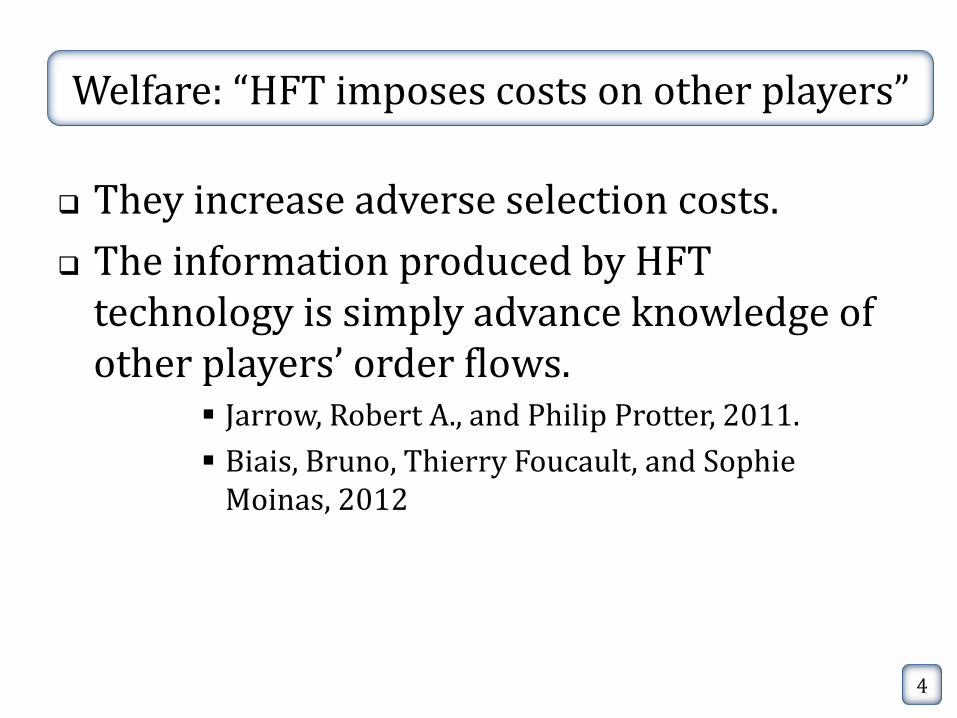
Welfare: “HFT imposes costs on other players”

They increase adverse selection costs.

The information produced by HFT technology is simply advance knowledge of other players’ order flows.

Jarrow, Robert A., and Philip Protter, 2011.

Biais, Bruno, Thierry Foucault, and Sophie Moinas, 2012

4

Welfare: “HFT improves market quality.”

Supported by most empirical studies that correlate HF measures/proxies with standard liquidity measures.

Hendershott, Terrence, Charles M. Jones, and Albert J. Menkveld, 2010

Hasbrouck, Joel, and Gideon Saar, 2011

Hendershott, Terrence J., and Ryan Riordan, 2012

5

“HFTs are efficient market-makers”

Empirical studies Kirilenko, Andrei A., Albert S. Kyle, Mehrdad Samadi, and

Tugkan Tuzun, 2010 Menkveld, Albert J., 2012 Brogaard, Jonathan, 2010a, 2010b, 2012

Strategy: identify a class of HFTs and analyze their trades.

HFTs closely monitor and manage their positions. HFTs often trade passively (supply liquidity via bid and

offer quotes) But …

HFTs don’t maintain a continuous market presence. They sometimes trade actively (“aggressively”)

6

Positioning

We use the term “high frequency trading” to refer to all sorts of rapid-paced market activity.

Most empirical analysis focuses on trades.

This study emphasizes quotes.

7

High-frequency quoting

Rapid oscillations of bid and/or ask quotes.

Example

AEPI is a small Nasdaq-listed manufacturing firm.

Market activity on April 29, 2011

National Best Bid and Offer (NBBO)

The highest bid and lowest offer (over all market centers)

8

9

National Best Bid and Offer for AEPI during regular trading hours

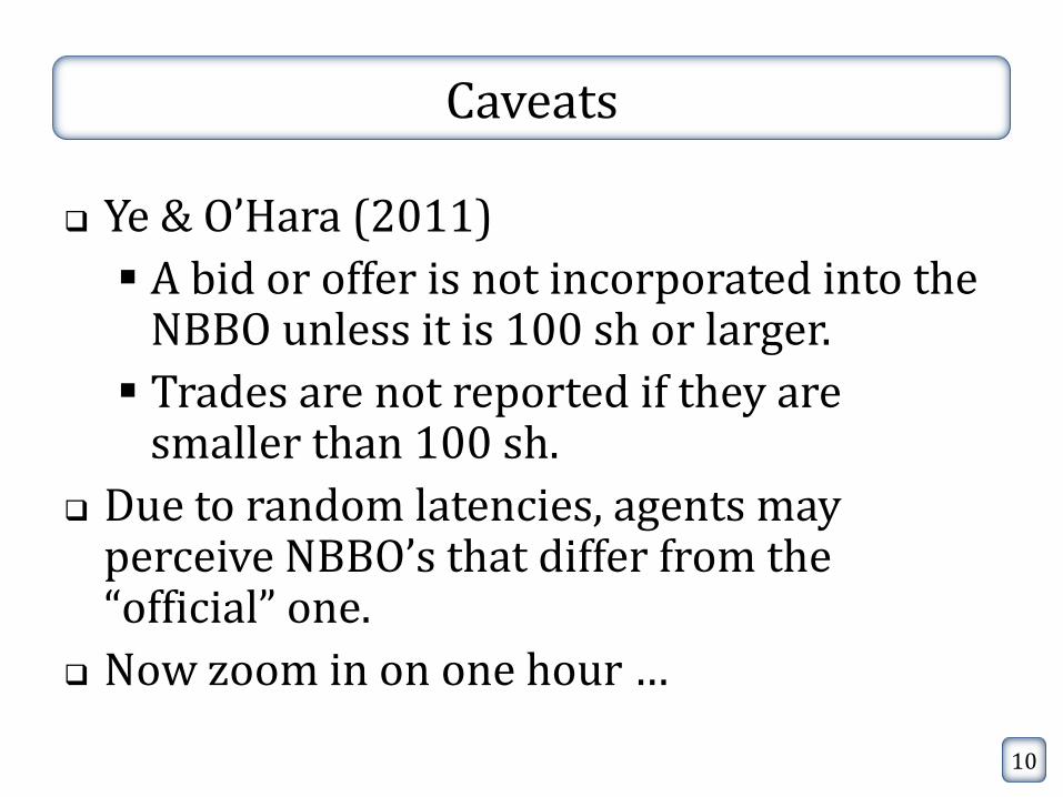
Caveats

Ye & O’Hara (2011)

A bid or offer is not incorporated into the NBBO unless it is 100 sh or larger.

Trades are not reported if they are smaller than 100 sh.

Due to random latencies, agents may perceive NBBO’s that differ from the “official” one.

Now zoom in on one hour …

10

11

National Best Bid and Offer for AEPI from 11:00 to 12:10

12

National Best Bid and Offer for AEPI from 11:15:00 to 11:16:00

13

National Best Bid and Offer for AEPI from 11:15:00 to 11:16:00

14

National Best Bid for AEPI: 11:15:21.400 to 11:15:21.800 (400 ms)

So what?

HFQ noise degrades the informational value of the bid and ask.

HFQ aggravates execution price uncertainty for marketable orders.

And in US equity markets …

NBBO used as reference prices for dark trades.

Top (and only the top) of a market’s book is protected against trade-throughs.

15

“Dark” Trades

Trades that don’t execute against a visible quote.

In many trades, price is assigned by reference to the NBBO.

Preferenced orders are sent to wholesalers.

Buys filled at NBO; sells at NBB.

Crossing networks match buyers and sellers at the midpoint of the NBBO.

16

Features of the AEPI episodes

Extremely rapid oscillations in the bid.

Start and stop abruptly

Possibly unconnected with fundamental news.

Directional (activity on the ask side is much smaller)

17

A framework for analysis: the requirements

Need precise resolution (the data have one ms. time-stamps)

Low-order vector autoregression?

Oscillations: spectral (frequency) analysis?

Represent a time series as a combination sine/cosine functions.

But the functions are recurrent over the full sample.

AEPI episodes are localized.

18

Stationarity

The oscillations are locally stationary.

Framework must pick up stationary local variation …

But not exclude random-walk components.

Should identify long-run components as well as short-run.

19

Intuitively, I’d like to …

Use a moving average to smooth series.

Implicitly estimating the long-term component.

Isolate the HF component as a residual.

20

Alternative: Time-scale decomposition

Represent a time-series in terms of basis functions (wavelets)

Wavelets:

Localized

Oscillatory

Use flexible (systematically varying) time-scales.

Accepted analytical tool in diverse disciplines.

Percival and Walden; Gencay et. al.

21

Sample bid path

22

0 2 4 6 82

0

2

4

6

8

10

First pass (level) transform

23

0 2 4 6 82

0

2

4

6

8

10 Original price series

2-period average

1-period detail

0 2 4 6 82

0

2

4

6

8

10

1-period detail

First pass (level) transform

24

0 2 4 6 82

0

2

4

6

8

10 Original price series

2-period average

1-period detail

1-period detail sum of squares

Second pass (level) transform

25 0 2 4 6 8

2

0

2

4

6

8

102-period average

2-period detail

4-period average

Third level (pass) transform

26

0 2 4 6 82

0

2

4

6

8

10

4-period average

4-period detail

8-period average

For each level 𝑗 = 1,2,… , we have …

A time scale, 𝜏𝑗 = 2𝑗−1

Higher level longer time scale.

𝜏𝑗 ∈ 1, 2, 4, …

“the persistence of the level-j component”

A scale-𝜏𝑗 “detail” component.

Centered (“zero mean”) series that tracks changes in the series at scale 𝜏𝑗 .

A scale-𝜏𝑗 sum of squares.

27

Interpretation

The full set of scale-𝜏𝑗 components

decomposes the original series into sequences ranging from “very choppy” to “very smooth”.

Multi-resolution analysis.

With additional structure, the full set of scale-𝜏𝑗 sums of squares corresponds to a

variance decomposition.

28

Multi-resolution analysis of AEPI bid

Data time-stamped to the millisecond.

Construct decomposition through level 𝐽 = 18.

For graphic clarity, aggregate the components into four groups.

Plots focus on 11am-12pm.

29

30

31

1-4ms

8ms-1s

2s-2m

>2m

Time scale

Connection to standard time series analysis

Suppose 𝑝𝑡 is a stochastic process

e.g., a random-walk

The scale-𝜏𝑗 sum-of-squares over the sample path (divided by n) defines an estimate of the wavelet variance.

Wavelet variance (and its estimate) are well-defined and well-behaved assuming that the first differences of 𝑝𝑡 are covariance stationary.

Wavelet decompositions are performed on the levels of 𝑝𝑡 not the first differences.

32

The wavelet variance of a random-walk

𝜈2 𝜏𝑗 ≡ wavelet variance at scale 𝜏𝑗

For a random-walk

𝑝𝑡 = 𝑝𝑡−1 + 𝑒𝑡 where 𝐸𝑒𝑡 = 0 and 𝐸𝑒𝑡

2 = 𝜎𝑒2

𝜈2 𝜏𝑗 = 𝜙 𝜏𝑗 𝜎𝑒2

where scaling factor 𝜙(𝜏𝑗) =1

6𝜏𝑗 +

1

2𝜏𝑗

𝜙(𝜏𝑗) ∈ 0.25, 0.38, 0.69, 1.3, 2.7, 5.3, 10.7, …

33

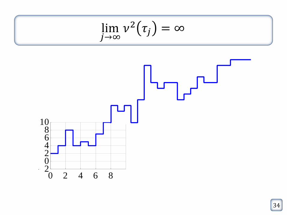
lim𝑗→∞

𝜈2 𝜏𝑗 = ∞

34

0 2 4 6 8202468

10

The wavelet variance for the AEPI bid: an economic interpretation

Orders sent to market are subject to random delays.

This leads to arrival uncertainty.

For a market order, this corresponds to price risk.

For a given time window, the wavelet variance measures this risk.

35

Timing a trade: the price path

36 5 10 15 20 25 30

Time

2

4

6

8Price

Timing a trade: the arrival window

37

The time-weighted average price (TWAP) benchmark

38

Time-weighted average price

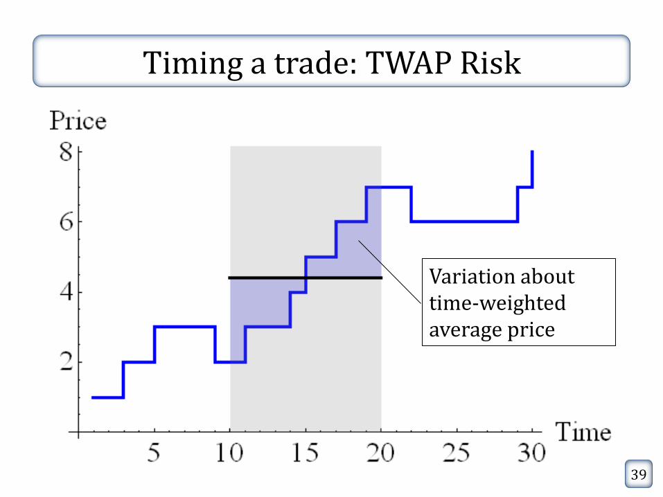
Timing a trade: TWAP Risk

39

Variation about time-weighted average price

The wavelet variance: a comparison with realized volatility

40

Data sample

100 US firms from April 2011

Sample stratified by equity market capitalization

Alphabetic sorting

Within each market cap decile, use first ten firms.

Summary data from CRSP

HF data from daily (“millisecond”) TAQ

41

Median

Share price, EOY 2010

Mkt cap, EOY, 2010, $Million

Avg daily dollar vol, 2010, $Thousand

Avg daily no. of trades, April 2011

Avg daily no. of quotes, April 2011

Full sample $13.75 420 2,140 1,111 23,347 Dollar Volume Deciles 0 (low) $4.18 30 20 17 846 1 $3.56 30 83 45 2,275 2 $3.70 72 228 154 5,309 3 $6.43 236 771 1,405 15,093 4 $7.79 299 1,534 468 15,433 5 $17.34 689 3,077 1,233 34,924 6 $26.34 1,339 5,601 2,045 37,549 7 $28.40 1,863 13,236 3,219 52,230 8 $36.73 3,462 34,119 7,243 94,842 9 (high) $44.58 18,352 234,483 25,847 368,579

Computational procedures

10 ℎ𝑟𝑠 × 60𝑚𝑖𝑛 × 60𝑠𝑒𝑐 × 1,000𝑚𝑠 = 3.6 × 107 “observations” (per series, per day)

Analyze data in rolling windows of ten minutes

Supplement millisecond-resolution analysis with time-scale decomposition of prices averaged over one-second.

Use maximal overlap discrete transforms with Daubechies(4) weights.

43

Example: AAPL (Apple Computer)

20 days

Regular trading hours are 9:30 to 16:00.

I restrict to 9:45 to 15:45

20 𝑑𝑎𝑦𝑠 × 6 ℎ𝑟𝑠 × 60 𝑚𝑖𝑛 = 7,200 𝑚𝑖𝑛

Compute 𝜈 2 𝜏𝑗 for 𝑗 = 1,… , 18

Time scales: 1ms to 131,072ms (about 2.2 minutes)

Tables report values for odd j (for brevity)

44

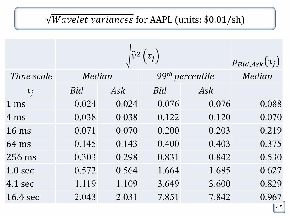
𝑊𝑎𝑣𝑒𝑙𝑒𝑡 𝑣𝑎𝑟𝑖𝑎𝑛𝑐𝑒𝑠 for AAPL (units: $0.01/sh)

45

𝜈 2 𝜏𝑗 𝜌𝐵𝑖𝑑,𝐴𝑠𝑘 𝜏𝑗

Time scale

𝜏𝑗

Median 99th percentile Median

Bid Ask Bid Ask

1 ms 0.024 0.024 0.076 0.076 0.088

4 ms 0.038 0.038 0.122 0.120 0.070

16 ms 0.071 0.070 0.200 0.203 0.219

64 ms 0.145 0.143 0.400 0.403 0.375

256 ms 0.303 0.298 0.831 0.842 0.530

1.0 sec 0.573 0.564 1.664 1.685 0.627

4.1 sec 1.119 1.109 3.649 3.600 0.829

16.4 sec 2.043 2.031 7.851 7.842 0.967

𝑪𝒖𝒎𝒖𝒍𝒂𝒕𝒊𝒗𝒆 𝒘𝒂𝒗𝒆𝒍𝒆𝒕 𝒗𝒂𝒓𝒊𝒂𝒏𝒄𝒆𝒔 for AAPL Bid (units: $0.01/sh)

46

𝜏𝑗 Median

99th

percentile

1 ms 0.024 0.076

4 ms 0.053 0.172

16 ms 0.103 0.302

64 ms 0.205 0.571

256 ms 0.423 1.153

1.0 sec 0.828 2.337

4.1 sec 1.621 4.857

16.4 sec 3.167 10.331

𝑪𝒖𝒎𝒖𝒍𝒂𝒕𝒊𝒗𝒆 𝒘𝒂𝒗𝒆𝒍𝒆𝒕 𝒗𝒂𝒓𝒊𝒂𝒏𝒄𝒆𝒔 for AAPL Bid (units: $0.01/sh)

47

𝜏𝑗 Median

99th

percentile

1 ms 0.024 0.076

4 ms 0.053 0.172

16 ms 0.103 0.302

64 ms 0.205 0.571

256 ms 0.423 1.153

1.0 sec 0.828 2.337

4.1 sec 1.621 4.857

16.4 sec 3.167 10.331

The price uncertainty for a trader who can only time his marketable trades within a 4-second window has 𝜎 = $0.016 Compare: current access fees ≈ $0.003

The wavelet correlation 𝜌𝑋,𝑌 𝜏𝑗

For two series X and Y, the wavelet variances are 𝜈𝑋2 𝜏𝑗

and 𝜈𝑌2 𝜏𝑗

The wavelet covariance is 𝜈𝑋,𝑌 𝜏𝑗

The wavelet correlation is

𝜌𝑋,𝑌 𝜏𝑗 =𝜈𝑋,𝑌 𝜏𝑗

𝜈𝑋2 𝜏𝑗 𝜈𝑌

2 𝜏𝑗

Fundamental value changes should affect both the bid and the ask.

The wavelet correlation at scale 𝜏𝑗 indicates the

contribution of fundamental volatility.

Next: wavelet correlation for AAPL bid and ask: 48

How closely do the wavelet variances for AAPL’s bid correspond to a random walk?

49

Scale Wavelet variance estimate

Random-walk variance factors

Implied random-walk variance

𝜏𝑗 𝜈 2 𝜏𝑗 𝜙 𝜏𝑗 𝜈 2 𝜏𝑗 𝜙 𝜏𝑗

1 ms 0.0009 0.1875 0.0050

4 ms 0.0024 0.4849 0.0049

16 ms 0.0075 1.8960 0.0039

64 ms 0.0309 7.5740 0.0041

256 ms 0.1360 30.2935 0.0045

1.0 sec 0.5140 121.1730 0.0042

4.1 sec 2.1434 484.6930 0.0044

16.4 sec 8.6867 1,938.7700 0.0045

Reasonable?

If 0.005 (cents per share)2 is the random-walk variance over one ms., the accumulated variance over a 6-hour mid-day period is:

0.005 × 1,000 × 3,600 × 6 = 108,000

The implied 6-hour standard deviation is about 329 (cents per share).

AAPL’s average price in the sample is about $340

3.29

340≈ 1%

50

Volatility Signature Plots

Suggested by Andersen and Bollerslev.

Plot realized volatility (per constant time unit) vs. length of interval used to compute the realized volatility.

Basic idea works for wavelet variances.

“How much is short-run quote volatility inflated, relative to what we’d expect from a random walk?”

51

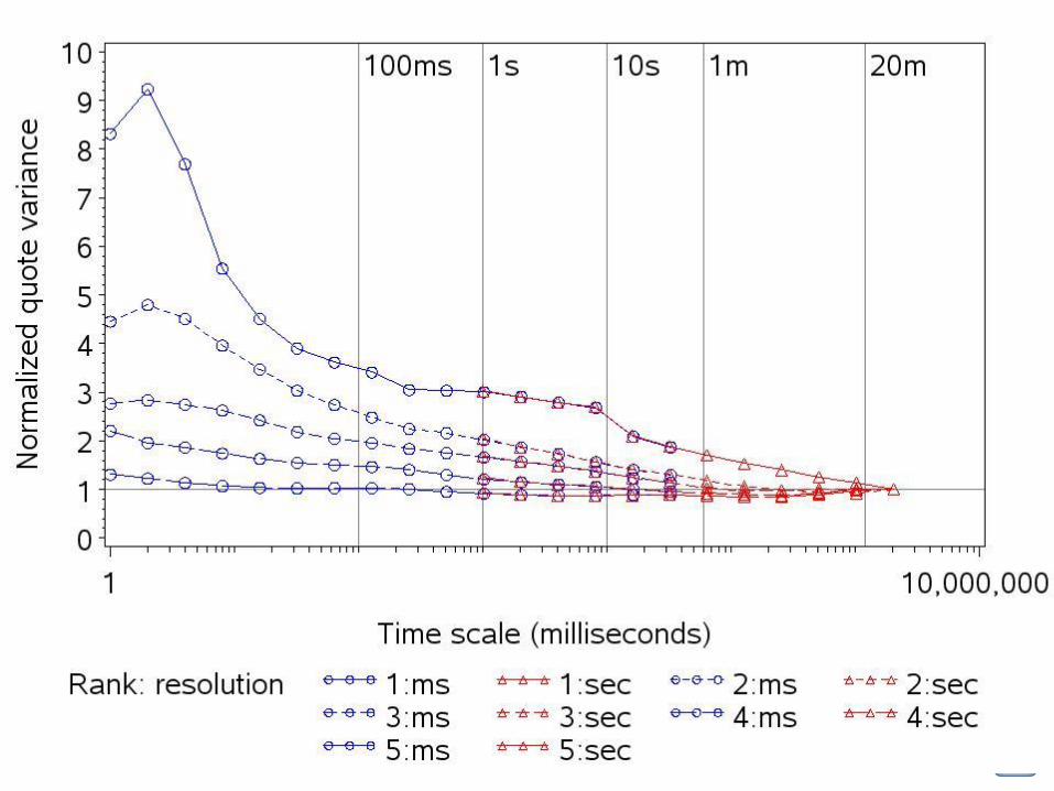
Normalization of wavelet variances

For a given stock, the implied random-walk variance at scale 𝜏𝑗 is 𝜈 2 𝜏𝑗 𝜙(𝜏𝑗) .

The longest time scale in the analysis is about 20 minutes.

The ratio 𝜈 2 𝜏𝑗 𝜙(𝜏𝑗)

𝜈 2 20 𝑚𝑖𝑛 𝜙(20 𝑚𝑖𝑛)

measures variance at scale 𝜏𝑗 relative to the wavelet variance at 20 minutes, under a random-walk benchmark.

If the price is truly a random walk, this should be unity for all 𝜏𝑗 .

52

For presentation …

Market cap deciles collapsed into quintiles.

Within each quintile, I average 𝜈 2 𝜏𝑗 𝜙(𝜏𝑗)

𝜈 2 20 𝑚𝑖𝑛 𝜙(20 𝑚𝑖𝑛) across firms.

Results from millisecond- and second-resolution analyses are spliced.

Next: the (normalized) volatility signature plot.

53

54

The take-away

For high-cap firms

Wavelet variances at short time scales have modest elevation relative to random-walk.

Low-cap firms

Wavelet variances are strongly elevated at short time scales.

Significant price risk relative to TWAP.

55

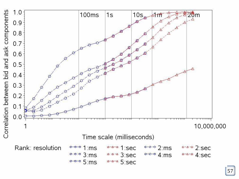
Sample bid-ask wavelet correlations

These are already normalized.

Compute quintile averages across firms.

56

57

How closely do movements in the bid and ask track?

Positive in all cases (!)

For high-cap stocks, 𝜌 ≈ 0.7 (one second) and 𝜌 > 0.9 (20 seconds)

For bottom cap-quintile, 𝜌 < 0.2 (one second) and 𝜌 < 0.5 (20 minutes)

58

A gallery

For each firm in mkt cap deciles 6, I examined the day with the highest wavelet variance at time scales of 1 second and under.

HFQ is easiest to see against a backdrop of low activity.

Next slides … some examples

59

60

61

62

63

64

65

66

Conclusions

High frequency quoting is a real (but episodic) fact of the market.

Time-scale decompositions are useful in measuring the overall effect.

… and detecting the episodes

Remaining questions …

67

Why does HFQ occur?

Why not? The costs are extremely low.

Testing?

Malfunction?

Interaction of simple algos?

Genuinely seeking liquidity (counterparty)?

Deliberately introducing noise?

Deliberately pushing the NBBO to obtain a favorable price in a dark trade?

68