High Energy X-ray and Gamma-ray Observations of Galaxy Clusters
169
WASHINGTON UNIVERSITY Department of Physics Dissertation Examination Committee: Henric Krawczynski, Chair James Buckley Ramanath Cowsik Sophia Hayes Charles Hohenburg Martin Israel Roger Phillips HIGH ENERGY X-RAY AND GAMMA-RAY OBSERVATIONS OF GALAXY CLUSTERS by Jeremy Shane Perkins A dissertation presented to the Graduate School of Arts and Sciences of Washington University in partial fulfillment of the requirements for the degree of Doctor of Philosophy April 2006 Saint Louis, Missouri
Transcript of High Energy X-ray and Gamma-ray Observations of Galaxy Clusters

WASHINGTON UNIVERSITY
Department of Physics
Dissertation Examination Committee:Henric Krawczynski, Chair
James BuckleyRamanath Cowsik
Sophia HayesCharles Hohenburg
Martin IsraelRoger Phillips
HIGH ENERGY X-RAY AND GAMMA-RAY OBSERVATIONS OF GALAXY
CLUSTERS
by
Jeremy Shane Perkins
A dissertation presented to theGraduate School of Arts and Sciences
of Washington University inpartial fulfillment of the
requirements for the degreeof Doctor of Philosophy
April 2006
Saint Louis, Missouri

Acknowledgements
I would first like to thank all those who have taught me through the years starting
with my mother and father who home-schooled me during elementary school and
supported me. I had wonderful math and science teachers in high school such as
Kathy Beck and Eric Unger who dedicated their time to teaching me to love the
physical sciences. This continued in college and I would not have gotten here today
without the guidance of Dr. Tommy Tarvin and Dr. Perry Tompkins who always
pushed me into doing more and better. Without the educational background that
these wonderful friends and teachers gave me, I would not be writing this now.
The most influential person to this work and my career has been my adviser, Dr.
Henric Krawczynski. Without his constant help and expertise this work could not
have been accomplished. Thank you very much for all of the time and energy you
have invested in me. In addition to Henric, Dr. James Buckley, Dr. Marty Israel and
Dr. Bob Binns have never failed to answer my questions or provided advice. I feel
honored to have been able to work with you.
I would also like to thank Trevor Weekes and the VERITAS1 collaboration for
1 The VERITAS Collaboration is supported by the U.S. Dept. of Energy, N.S.F., the SmithsonianInstitution, P.P.A.R.C. (U.K.), N.S.E.R.C. (Canada), and Enterprise-Ireland.
ii
providing me with data and feedback. The Dean of the Graduate School of Arts
and Sciences at Washington University generously provided me with a Dissertation
Fellowship to enable me to complete this thesis on time. Dr. Martin Hardcastle also
provided valuable assistance in the analysis of the XMM data.
Graduate school could not be done without graduate students in more ways than
one: graduate students are not only the workhorses of academia but they are also
friends, peers and relief valves. There is an accumulated knowledge that is carried
around in graduate students’ heads that is passed on from student to student and
these people have given me much: Karl Kosack, Lauren Scott, Scott Hughes, Paul
Rebillot, Brian Raugh, Kris Gutierrez, Kuen “Vicky” Lee, Trey Garson, Christopher
Aubin, Kelley Lave, Tom Mitchel, Weylin McMillin, and many more. Thank you for
everything.
Many other people in the department were vital to my research and life in gen-
eral and have taught me everything from electronics and shop to the intricacies of
academia as well as physics: Paul Dowkontt, Ira Jung, Richard Bose, Dana Braun,
Marty Olevitch, Garry Simburger, Denny Huelsman, Tony Biondo, Todd Hardt,
Sarah Jordan, Julia Hamilton, Christine Monteith, Jamie Eikmeier and Allison Ver-
beck.
I would like to thank my friends and neighbors who have really made St. Louis
my home for these past five years. Ellen, thank you for editing many of these pages.
I thank my friends at La Dolce Via for providing the espresso, food and wine that
has spoiled my taste buds for years to come.
iii

Finally, I would like to thank my wife Donna for following me to St. Louis and
always being there for me. Thank you for thoroughly editing my thesis; usually you
can only take so much of me talking Physics but here you endured over a hundred
pages of it in a very short amount of time. I could not have done it without you.
iv
Contents
Acknowledgements ii
List of Figures ix
List of Tables x
Abstract xi
Copyright xiii
1 Overview 1
2 Introduction 42.1 Three Archetypical Galaxy Clusters . . . . . . . . . . . . . . . . . . . 6
2.1.1 The Perseus Cluster . . . . . . . . . . . . . . . . . . . . . . . 62.1.2 Abell 2029 . . . . . . . . . . . . . . . . . . . . . . . . . . . . . 102.1.3 3C 129 . . . . . . . . . . . . . . . . . . . . . . . . . . . . . . . 12
2.2 The X-Ray and Gamma-Ray Astrophysics of Galaxy Clusters . . . . 132.2.1 Thermal Bremsstrahlung . . . . . . . . . . . . . . . . . . . . . 142.2.2 Thermal and Non-Thermal Particles in Clusters . . . . . . . . 172.2.3 Possible MeV Gamma-Ray Emission . . . . . . . . . . . . . . 182.2.4 VHE Gamma-Ray Emission Mechanisms . . . . . . . . . . . . 192.2.5 Extragalactic Extinction . . . . . . . . . . . . . . . . . . . . . 222.2.6 Cooling Flows . . . . . . . . . . . . . . . . . . . . . . . . . . . 25
3 X-Ray and Gamma-Ray Observatories 293.1 X-Ray Observatories . . . . . . . . . . . . . . . . . . . . . . . . . . . 29
3.1.1 Solid State Detectors . . . . . . . . . . . . . . . . . . . . . . . 303.1.2 XMM-Newton . . . . . . . . . . . . . . . . . . . . . . . . . . . 31
MOS X-ray CCDs . . . . . . . . . . . . . . . . . . . . . . . . 32PN X-ray CCDs . . . . . . . . . . . . . . . . . . . . . . . . . . 33Optical . . . . . . . . . . . . . . . . . . . . . . . . . . . . . . . 34
3.1.3 Chandra . . . . . . . . . . . . . . . . . . . . . . . . . . . . . . 353.2 The Whipple Gamma-Ray Observatory . . . . . . . . . . . . . . . . . 36
3.2.1 The Imaging Atmospheric Cherenkov Technique . . . . . . . . 37
v
Contents
3.2.2 The Whipple 10 m Telescope . . . . . . . . . . . . . . . . . . 44
4 XMM-Newton X-ray Observations of 3C 129 474.1 Data Sets and Analysis . . . . . . . . . . . . . . . . . . . . . . . . . . 504.2 Radio Tail Results . . . . . . . . . . . . . . . . . . . . . . . . . . . . 564.3 Spectra . . . . . . . . . . . . . . . . . . . . . . . . . . . . . . . . . . 604.4 Optical Monitor Analysis and Results . . . . . . . . . . . . . . . . . . 614.5 Discussion . . . . . . . . . . . . . . . . . . . . . . . . . . . . . . . . . 62
5 TeV Observations of the Perseus and A2029 Clusters with the Whip-ple 10 m Telescope 645.1 Data and Analysis . . . . . . . . . . . . . . . . . . . . . . . . . . . . 64
5.1.1 Instrumentation and Data Sets . . . . . . . . . . . . . . . . . 655.1.2 Standard Analysis . . . . . . . . . . . . . . . . . . . . . . . . 675.1.3 Cluster Specific Analysis . . . . . . . . . . . . . . . . . . . . . 67
5.2 Results . . . . . . . . . . . . . . . . . . . . . . . . . . . . . . . . . . . 735.3 Interpretation and Discussion . . . . . . . . . . . . . . . . . . . . . . 76
6 Detector Development 806.1 EXIST . . . . . . . . . . . . . . . . . . . . . . . . . . . . . . . . . . . 816.2 Equipment . . . . . . . . . . . . . . . . . . . . . . . . . . . . . . . . . 836.3 Measurements . . . . . . . . . . . . . . . . . . . . . . . . . . . . . . . 846.4 Cs137 Spectra . . . . . . . . . . . . . . . . . . . . . . . . . . . . . . . 856.5 Simulations and Comparison to Experimental Results . . . . . . . . . 896.6 Summary and Outlook . . . . . . . . . . . . . . . . . . . . . . . . . . 92
7 Conclusions 947.1 Future Cluster Observations . . . . . . . . . . . . . . . . . . . . . . . 96
7.1.1 NuSTAR and GLAST . . . . . . . . . . . . . . . . . . . . . . 977.2 VERITAS and H.E.S.S. . . . . . . . . . . . . . . . . . . . . . . . . . 98
A 3C 129 Observation Summary 101
B Whipple 10m Run Summary 106
C I-V Measurements 108C.1 Standard Measurements . . . . . . . . . . . . . . . . . . . . . . . . . 108
C.1.1 Apparatus . . . . . . . . . . . . . . . . . . . . . . . . . . . . . 108C.1.2 LabView Program . . . . . . . . . . . . . . . . . . . . . . . . 110
C.2 Four Point Measurements . . . . . . . . . . . . . . . . . . . . . . . . 118C.2.1 Apparatus . . . . . . . . . . . . . . . . . . . . . . . . . . . . . 119C.2.2 Data . . . . . . . . . . . . . . . . . . . . . . . . . . . . . . . . 119C.2.3 Analysis . . . . . . . . . . . . . . . . . . . . . . . . . . . . . . 121
vi
Contents
D Data Acquisition System for X-ray Spectroscopy 124D.1 Apparatus . . . . . . . . . . . . . . . . . . . . . . . . . . . . . . . . . 124D.2 Code . . . . . . . . . . . . . . . . . . . . . . . . . . . . . . . . . . . . 124
E Upper Limit Calculation 144E.1 Code . . . . . . . . . . . . . . . . . . . . . . . . . . . . . . . . . . . . 144
vii

List of Figures
2.1 Optical Image of the Perseus Cluster . . . . . . . . . . . . . . . . . . 72.2 Hubble Image of NGC1275 . . . . . . . . . . . . . . . . . . . . . . . . 82.3 Radio Image of 3C 84 . . . . . . . . . . . . . . . . . . . . . . . . . . . 92.4 Chandra Image of the Perseus Cluster . . . . . . . . . . . . . . . . . 102.5 Abell 2029 X-ray and Radio . . . . . . . . . . . . . . . . . . . . . . . 112.6 Cluster Iron Lines . . . . . . . . . . . . . . . . . . . . . . . . . . . . . 162.7 Extragalactic Background Light . . . . . . . . . . . . . . . . . . . . . 232.8 Extragalactic Background Light Absorption . . . . . . . . . . . . . . 25
3.1 XMM-Newton Mirrors . . . . . . . . . . . . . . . . . . . . . . . . . . 313.2 XMM-Newton . . . . . . . . . . . . . . . . . . . . . . . . . . . . . . . 323.3 XMM-Newton MOS Quantum Efficiency . . . . . . . . . . . . . . . . 333.4 XMM-Newton PN Quantum Efficiency . . . . . . . . . . . . . . . . . 343.5 Chandra ACIS Quantum Efficiency . . . . . . . . . . . . . . . . . . . 363.6 The Whipple 10m IACT . . . . . . . . . . . . . . . . . . . . . . . . . 373.7 Gamma-ray Shower . . . . . . . . . . . . . . . . . . . . . . . . . . . . 383.8 Dialectric Medium . . . . . . . . . . . . . . . . . . . . . . . . . . . . 403.9 Cherenkov Radiation . . . . . . . . . . . . . . . . . . . . . . . . . . . 403.10 Electromagnetic Cascades . . . . . . . . . . . . . . . . . . . . . . . . 433.11 Images of Showers . . . . . . . . . . . . . . . . . . . . . . . . . . . . . 453.12 Whipple Camera . . . . . . . . . . . . . . . . . . . . . . . . . . . . . 46
4.1 Sources near 3C 129 . . . . . . . . . . . . . . . . . . . . . . . . . . . 494.2 ICM Pressure . . . . . . . . . . . . . . . . . . . . . . . . . . . . . . . 494.3 3C 129 Raw Image . . . . . . . . . . . . . . . . . . . . . . . . . . . . 524.4 3C 129 Image Range 6 . . . . . . . . . . . . . . . . . . . . . . . . . . 544.5 3C 129 Large Jet . . . . . . . . . . . . . . . . . . . . . . . . . . . . . 574.6 3C 129 Small Jet . . . . . . . . . . . . . . . . . . . . . . . . . . . . . 574.7 3C 129 X-ray Profile . . . . . . . . . . . . . . . . . . . . . . . . . . . 584.8 Full Frame Optical Image of 3C 129 . . . . . . . . . . . . . . . . . . . 624.9 User Window Optical Image of 3C 129 . . . . . . . . . . . . . . . . . 63
5.1 Cosmic Ray Counts . . . . . . . . . . . . . . . . . . . . . . . . . . . . 665.2 Optimal Cuts . . . . . . . . . . . . . . . . . . . . . . . . . . . . . . . 69
viii

List of Figures
5.3 Crab Rates . . . . . . . . . . . . . . . . . . . . . . . . . . . . . . . . 705.4 Events vs. Arrival Direction . . . . . . . . . . . . . . . . . . . . . . . 725.5 Expected Counts . . . . . . . . . . . . . . . . . . . . . . . . . . . . . 735.6 Perseus Upper Limit Map . . . . . . . . . . . . . . . . . . . . . . . . 745.7 A2029 Upper Limit Map . . . . . . . . . . . . . . . . . . . . . . . . . 755.8 Perseus and A2029 Flux . . . . . . . . . . . . . . . . . . . . . . . . . 78
6.1 EXIST . . . . . . . . . . . . . . . . . . . . . . . . . . . . . . . . . . . 826.2 Coded Mask . . . . . . . . . . . . . . . . . . . . . . . . . . . . . . . . 826.3 CZT Pulse Shape Analysis . . . . . . . . . . . . . . . . . . . . . . . . 866.4 Cs137 Spectrum Anode vs. Cathode . . . . . . . . . . . . . . . . . . . 876.5 Charge Corrected Cs137 spectrum . . . . . . . . . . . . . . . . . . . . 876.6 Cs137 spectrum Anode charge versus Drift Time . . . . . . . . . . . . 886.7 Drift Time Corrected Cs137 Spectrum . . . . . . . . . . . . . . . . . . 886.8 Graphical representation of the simulation model . . . . . . . . . . . 906.9 Comparison of Simulated and Experimental Data. . . . . . . . . . . . 916.10 Charge Induced vs. Starting Position . . . . . . . . . . . . . . . . . . 92
7.1 NuSTAR Effective Area . . . . . . . . . . . . . . . . . . . . . . . . . 987.2 Cluster Flux with VERITAS and GLAST Sensitivity . . . . . . . . . 99
C.1 Detector I-V Curves . . . . . . . . . . . . . . . . . . . . . . . . . . . 109C.2 I-V Schematic . . . . . . . . . . . . . . . . . . . . . . . . . . . . . . . 111C.3 Front Panel Diagram . . . . . . . . . . . . . . . . . . . . . . . . . . . 114C.4 I-V Block Diagram 1 . . . . . . . . . . . . . . . . . . . . . . . . . . . 115C.5 I-V Block Diagram 2 . . . . . . . . . . . . . . . . . . . . . . . . . . . 116C.6 I-V Block Diagram 1 . . . . . . . . . . . . . . . . . . . . . . . . . . . 117C.7 Four Point Schematic . . . . . . . . . . . . . . . . . . . . . . . . . . . 120C.8 Four Point Results . . . . . . . . . . . . . . . . . . . . . . . . . . . . 123
D.1 DAQ Schmatic . . . . . . . . . . . . . . . . . . . . . . . . . . . . . . 125D.2 Pixel Layout . . . . . . . . . . . . . . . . . . . . . . . . . . . . . . . . 126
ix
List of Tables
2.1 EGRET Upper Limits . . . . . . . . . . . . . . . . . . . . . . . . . . 18
4.1 XMM Energy Bins . . . . . . . . . . . . . . . . . . . . . . . . . . . . 534.2 Deficit Upper Limits . . . . . . . . . . . . . . . . . . . . . . . . . . . 594.3 Deficit Estimates . . . . . . . . . . . . . . . . . . . . . . . . . . . . . 594.4 3C 129 Spectra . . . . . . . . . . . . . . . . . . . . . . . . . . . . . . 61
5.1 Perseus and A2029 Datasets . . . . . . . . . . . . . . . . . . . . . . . 665.2 King Profile Parameters . . . . . . . . . . . . . . . . . . . . . . . . . 715.3 Radio Sources Within Clusters . . . . . . . . . . . . . . . . . . . . . . 745.4 Upper Limits . . . . . . . . . . . . . . . . . . . . . . . . . . . . . . . 76
A.1 0146490101 Observation Data File Summary . . . . . . . . . . . . . . 101A.2 3C 129 Proposal Target Information . . . . . . . . . . . . . . . . . . . 102A.3 3C 129 Observation Record . . . . . . . . . . . . . . . . . . . . . . . 102A.4 3C 129 Instrument Information . . . . . . . . . . . . . . . . . . . . . 102A.5 3C 129 Esposure and Configuration Information . . . . . . . . . . . . 103
B.1 Perseus Run Summary . . . . . . . . . . . . . . . . . . . . . . . . . . 106B.2 Abell 2029 Run Summary . . . . . . . . . . . . . . . . . . . . . . . . 107
C.1 I-V Equipment . . . . . . . . . . . . . . . . . . . . . . . . . . . . . . 110C.2 I-V Connections . . . . . . . . . . . . . . . . . . . . . . . . . . . . . . 112C.3 Four Point Data . . . . . . . . . . . . . . . . . . . . . . . . . . . . . . 120C.4 Four Point Results 1 . . . . . . . . . . . . . . . . . . . . . . . . . . . 122C.5 Four Point Results 2 . . . . . . . . . . . . . . . . . . . . . . . . . . . 122
x

Abstract
Galaxy clusters are the largest and most massive gravitationally bound systems in
the Universe. Galaxy clusters are bright sources of X-rays owing to thermal emission
of the hot intracluster medium. Furthermore, galaxy clusters might be sources of TeV
gamma rays emitted by non-thermal high-energy protons and electrons accelerated
by large scale structure formation shocks, galactic winds, or active galactic nuclei. In
addition, gamma rays may be produced in dark matter particle annihilation processes
at the cluster cores. I report on observations of the galaxy cluster 3C 129 with the
XMM-Newton X-ray observatory. These observations have two major aims. First, I
search for interactions of the nonthermal plasma of the large head-tail radio galaxy
3C 129 with the thermal intracluster medium. Second, I study the X-ray emission
from the core of the radio galaxy. I derive an upper limit on the deficit in the
ICM plasma due to the interacting radio jet which is less than the expected 10%.
Additionally, I find an excess in the core emission over the Chandra observations,
suggesting the presence of extended emission near the core. I also report on the
search for TeV emission from the galaxy clusters Perseus and Abell 2029 using the
10 m Whipple Cherenkov telescope during the 2003-2004 and 2004-2005 observing
xi

List of Tables
seasons. I apply a two-dimensional analysis technique to scrutinize the clusters for
TeV emission, first determining flux upper limits on TeV gamma-ray emission from
point sources within the clusters then deriving upper limits on the extended cluster
emission. I subsequently compare the flux upper limits with EGRET upper limits at
100 MeV and theoretical models. Assuming that the gamma-ray surface brightness
profile mimics that of the thermal X-ray emission and that the spectrum of cluster
cosmic rays extends all the way from thermal energies to multi-TeV energies with a
differential spectral index of -2.1, the results imply that the cosmic ray proton energy
density is less than 7.9% of the thermal energy density for the Perseus cluster.
xii

This work is licensed under the Creative Commons
Attribution-NonCommercial-ShareAlike2.5 License.
To view a copy of this license, visit
http://creativecommons.org/licenses/by-nc-sa/2.5/
or send a letter to
Creative Commons,
543 Howard Street, 5th Floor,
San Francisco, California, 94105, USA.
Chapter 1
Overview
Galaxy clusters are the largest and most massive gravitationally bound structures
in the Universe. The most important components of galaxy clusters are (i) a dark
matter halo which defines the gravitational potential of the cluster, (ii) the intracluster
medium which contains the major fraction of the cluster barions and consists of hot
thermal gas, cosmic rays and magnetic fields, and (iii) galaxies which move in the
dark matter potential and contain most of the stars of the cluster.
In this thesis, I studied clusters with the X-ray observatory XMM-Newton and
the Whipple 10m gamma-ray telescope. I combined XMM-Newton observations of
the galaxy cluster 3C 129 (named after the radio galaxy it contains) with radio
observations of the archetypical head-tail radio galaxy 3C 129 to study the interaction
of the plasma of the radio galaxy with the intracluster medium. For this purpose, I
conducted a search for cavities in the X-ray emitting gas. Furthermore, I scrutinized
the X-ray emission from the head of the radio galaxy searching for evidence of emission
1

from shocked gas ahead of the radio core. The results constrain the nature of the
radio emitting plasma in the tail of the radio galaxy and the interaction of the radio
galaxy with the cluster gas.
As part of the VERITAS collaboration, I observed the Perseus and Abell 2029
galaxy clusters with the Whipple 10m Cherenkov telescope. While X-ray observa-
tions give information about the hot thermal gas, gamma-ray observations allow us
to study non-thermal high-energy particle populations. In particular, TeV gamma-ray
observations make it possible to search for ”Cosmological Cosmic Rays” that accumu-
late over the total lifetime of the clusters. Combining the TeV gamma-ray observa-
tions with archival X-ray observations allowed me to constrain the ratio between the
intracluster energy density in thermal plasma and in the non-thermal Cosmological
Cosmic Rays. I complemented the cluster observations with observations of the Crab
Nebula (a steady well calibrated source of TeV gamma-rays) at different locations in
the field of view of the telescope and with Monte Carlo simulations to determine the
sensitivity of the Whipple telescope for extended sources.
In addition to analyzing data, I worked on the development of Cadmium Zinc
Telluride (CZT) detectors. CZT is a high-Z large bandgap semiconductor for the
room-temperature detection of hard X-rays. CZT detectors find application in space-
borne X-ray astronomy, medical imaging, and homeland security devices. Owing its
good energy resolution and excellent spatial resolution, CZT detectors are expected to
play an important role in many future space-based X-ray missions, as the hard X-ray
detectors on board of Constellation-X, NuSTAR and EXIST. I used CZT substrates
2

from a variety of manufacturers to test the effects of different contact-materials using
electron beam deposition. I programmed the data acquisition with a 500 MHz oscillo-
scope and set up a four point measurement of the surface conductivity. Furthermore,
I evaluated the possibility to correct the charge measured at the pixels of the detector
for the depth of the interaction below pixels.
The rest of the thesis is structured as follows: I will first introduce the astrophysics
of galaxy clusters, focusing on their very high energy emission (Chapter 2). In Chapter
3, I will give an overview of the observatories used to acquire the results obtained in
my thesis. Following this, I describe the X-ray observations of the galaxy cluster 3C
129 in Chapter 4 and the TeV gamma-ray observations of the Perseus and Abell 2029
galaxy clusters in Chapter 5. I describe the results of the CZT research in Chapter 6.
I conclude with a discussion of future directions in the study of gamma-ray emission
from galaxy clusters and future X-ray and gamma-ray observatories in Chapter 7.
In Appendices A and B, I summarize the properties of the XMM data set and the
Whipple 10m data sets, respectively. In Appendix C, I describe the I-V measurement
set-up. In Appendices D and E, I describe the CZT data acquisition system and the
method used to derive upper limits.
3

Chapter 2
Introduction
The phenomenology of galaxy clusters spans an enormous range in sizes and time
scales. Clusters can contain hundreds of individual galaxies that are gravitationally
bound to a large central cusp of dark matter. The most massive clusters are the
largest gravitationally bound objects in the universe and can contain up to 1015M
down to the smallest clusters with only 1010M. The closest massive clusters are
the Virgo, Perseus and Coma clusters at distances of 16, 75, and 99 Mpc from us.
The most distant cluster detected so far is RDCS0848.6+4453 at a redshift of 1.24
(Rosati et al., 2004). The intra-cluster medium (ICM) of a cluster, made up of an
optically thin hot gas, has more mass than all the cluster galaxies together. Clusters
are additionally a promising testing ground for dark matter studies since they are
thought to form around a large central dark matter cusp.
Clusters of galaxies have inspired intensive astrophysical study at all wavelengths.
Clusters are ideal cosmological laboratories and allow for the study of structure for-
4

mation, dark matter and cosmology. With the advent of High Energy Astrophysics
a new window of cluster research has been opened with spectacular results coming
from the X-ray observatories, Einstein (or HEAO-2, launched in 1981) then ROSAT
(launched in 1990) and ASCA (or Astro-D, launched in 1993). These early observato-
ries provided a wealth of information about the composition and structure of clusters.
The next generation of imaging-spectrometer observatories (the early satellites were
either spectrometers or imagers but not both), Chandra and XMM-Newton (both
launched in 1999) expanded on this by incorporating the best aspects of the previous
generation. Multiwavelength studies of clusters using radio, microwave, optical and
X-ray bands allow astrophysicists to observe interactions of thermal and non-thermal
plasmas, and to study the magnetic field.
In this theses, I present Very High Energy (VHE)1 observations of two galaxy
clusters, Perseus and Abell 2029 and Low Energy (LE) 2 observations of the galaxy
cluster, 3C 129. The addition of new tools is constantly needed to provide improved
results and I will describe several recent instruments and developments in the field of
High Energy astrophysics. In galaxy clusters, collisionless structure formation shocks
are thought to be the main agents responsible for heating the ICM to temperatures
of kBT'10 keV. Through this and other processes, gravitational energy is converted
into the random kinetic energy of non-thermal baryons (protons) and leptons (elec-
trons). Galactic winds (Volk and Atoyan, 1999) and re-acceleration of mildly rel-
1 100 GeV - 100 TeV
2 0.1 keV - 10 keV
5

2.1 Three Archetypical Galaxy Clusters
ativistic particles injected into the ICM by powerful cluster members (Enßlin and
Biermann, 1998) may accelerate additional particles to non-thermal energies. Using
galactic cosmic rays (CR) as a yard stick, one expects that the energy density of cos-
mic ray protons (CRp) dominates over cosmic ray electrons (CRe) by approximately
two orders of magnitude, and may be comparable to thermal particles and the ICM
magnetic field. CRp can divisively escape clusters only on time scales much longer
than the Hubble time. Therefore, they accumulate over the entire formation history
(Volk and Atoyan, 1999).
2.1 Three Archetypical Galaxy Clusters
2.1.1 The Perseus Cluster
The Perseus cluster of galaxies3 (Abell 426 or Perseus A) within the Perseus
constellation is at a distance of 75 Mpc (z = 0.0179) from us and has a total mass of
4×10¹⁴ M; making it one of the largest and closest galaxy clusters (Girardi et al.,
1998). As such, it is one of the most studied clusters at all wavelengths and has
provided some interesting results.
Optical
The Perseus cluster is one of the largest objects in the sky and numerous optical
studies of the cluster exist (see Figure 2.1 for an example). The Central Dominant
(CD) galaxy, NGC 1275, was one of the prototypical group of six galaxies studied by
3 RA: 03h 19m 13s Dec: 41d 33’ 00” Epoch 2000
6
2.1 Three Archetypical Galaxy Clusters
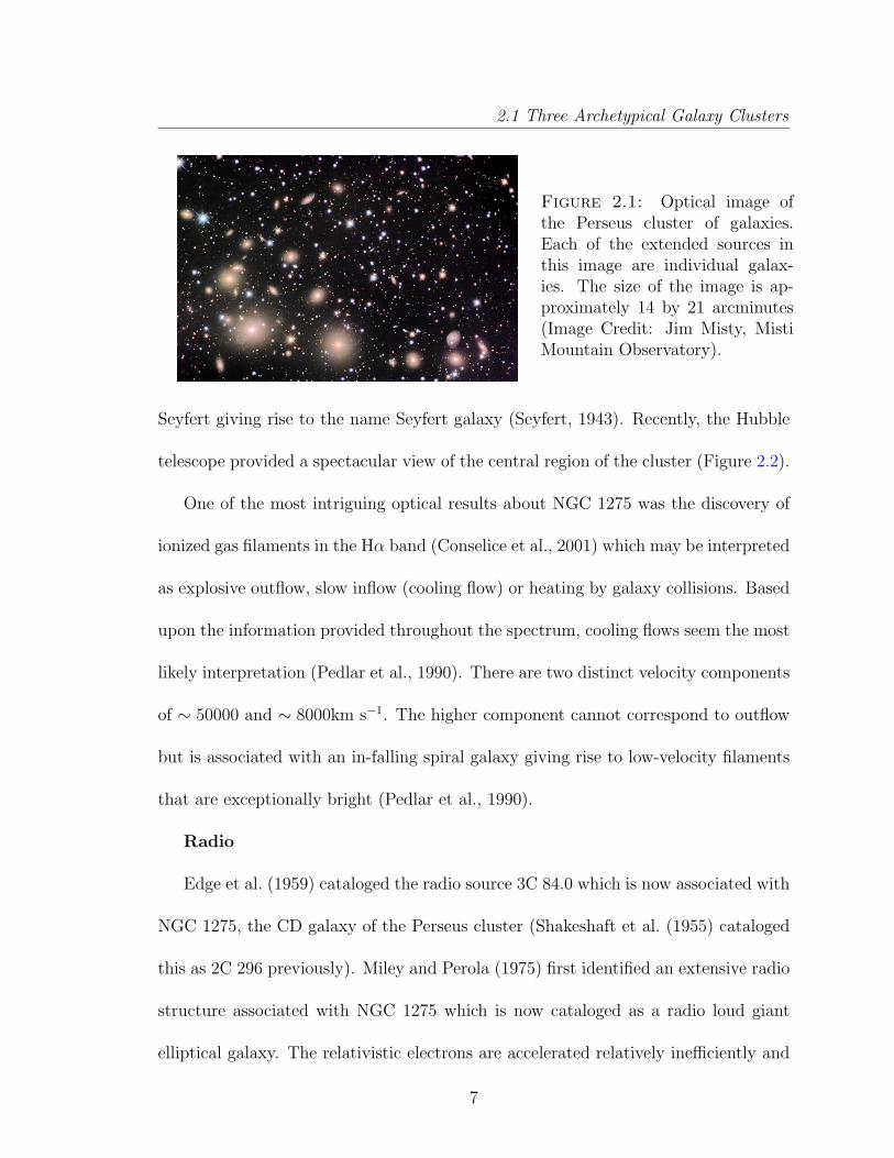
Figure 2.1: Optical image ofthe Perseus cluster of galaxies.Each of the extended sources inthis image are individual galax-ies. The size of the image is ap-proximately 14 by 21 arcminutes(Image Credit: Jim Misty, MistiMountain Observatory).
Seyfert giving rise to the name Seyfert galaxy (Seyfert, 1943). Recently, the Hubble
telescope provided a spectacular view of the central region of the cluster (Figure 2.2).
One of the most intriguing optical results about NGC 1275 was the discovery of
ionized gas filaments in the Hα band (Conselice et al., 2001) which may be interpreted
as explosive outflow, slow inflow (cooling flow) or heating by galaxy collisions. Based
upon the information provided throughout the spectrum, cooling flows seem the most
likely interpretation (Pedlar et al., 1990). There are two distinct velocity components
of ∼ 50000 and ∼ 8000km s−1. The higher component cannot correspond to outflow
but is associated with an in-falling spiral galaxy giving rise to low-velocity filaments
that are exceptionally bright (Pedlar et al., 1990).
Radio
Edge et al. (1959) cataloged the radio source 3C 84.0 which is now associated with
NGC 1275, the CD galaxy of the Perseus cluster (Shakeshaft et al. (1955) cataloged
this as 2C 296 previously). Miley and Perola (1975) first identified an extensive radio
structure associated with NGC 1275 which is now cataloged as a radio loud giant
elliptical galaxy. The relativistic electrons are accelerated relatively inefficiently and
7

2.1 Three Archetypical Galaxy Clusters
Figure 2.2: Hubble image takenwith the Wide Field PlanetaryCamera 2 showing traces of spiralstructure with dust lanes and blueactive star forming regions. Thesefeatures are taken as evidence thata spiral galaxy is falling in to theCD elliptical galaxy NGC 1275.
may significantly contribute to the production of the thermal X-ray emitting gas
(Pedlar et al., 1990). Recent observations by Romney et al. (1996) using VLBI have
displayed several unusual features including a counter-jet. See Figure 2.3 for an
example of the structure seen with radio observations.
X-Ray
The Perseus cluster is the brightest X-ray cluster in the sky and has been studied
by all X-ray telescopes (Fabian et al., 1974, 1981) and labeled as the prototypical
Cooling Flow Galaxy cluster (see Section below). The X-ray emission is mainly
due to thermal bremsstrahlung and line radiation (typical for clusters) from the hot
ICM and is centered on NCG 1275. The emission is highly peaked towards this CD
galaxy and ROSAT and Chandra observations have shown that radio sources can
inflate bubbles in the intracluster medium. Radio plasma replacing hot ICM has
been detected as cavities in the ICM X-ray surface brightness distribution. Fabian
8
2.1 Three Archetypical Galaxy Clusters
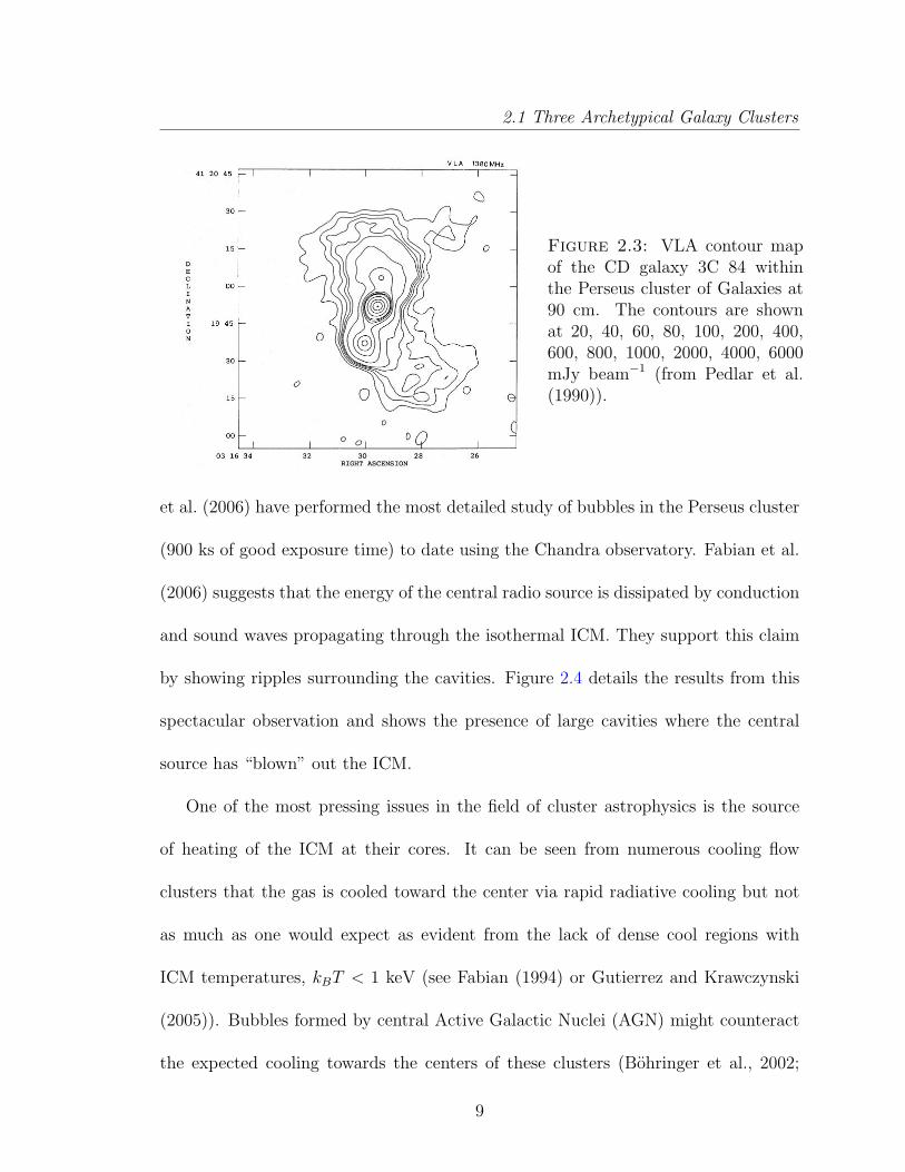
Figure 2.3: VLA contour mapof the CD galaxy 3C 84 withinthe Perseus cluster of Galaxies at90 cm. The contours are shownat 20, 40, 60, 80, 100, 200, 400,600, 800, 1000, 2000, 4000, 6000mJy beam−1 (from Pedlar et al.(1990)).
et al. (2006) have performed the most detailed study of bubbles in the Perseus cluster
(900 ks of good exposure time) to date using the Chandra observatory. Fabian et al.
(2006) suggests that the energy of the central radio source is dissipated by conduction
and sound waves propagating through the isothermal ICM. They support this claim
by showing ripples surrounding the cavities. Figure 2.4 details the results from this
spectacular observation and shows the presence of large cavities where the central
source has “blown” out the ICM.
One of the most pressing issues in the field of cluster astrophysics is the source
of heating of the ICM at their cores. It can be seen from numerous cooling flow
clusters that the gas is cooled toward the center via rapid radiative cooling but not
as much as one would expect as evident from the lack of dense cool regions with
ICM temperatures, kBT < 1 keV (see Fabian (1994) or Gutierrez and Krawczynski
(2005)). Bubbles formed by central Active Galactic Nuclei (AGN) might counteract
the expected cooling towards the centers of these clusters (Bohringer et al., 2002;
9
2.1 Three Archetypical Galaxy Clusters
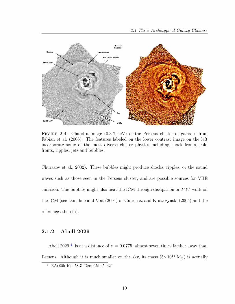
Figure 2.4: Chandra image (0.3-7 keV) of the Perseus cluster of galaxies fromFabian et al. (2006). The features labeled on the lower contrast image on the leftincorporate some of the most diverse cluster physics including shock fronts, coldfronts, ripples, jets and bubbles.
Churazov et al., 2002). These bubbles might produce shocks, ripples, or the sound
waves such as those seen in the Perseus cluster, and are possible sources for VHE
emission. The bubbles might also heat the ICM through dissipation or PdV work on
the ICM (see Donahue and Voit (2004) or Gutierrez and Krawczynski (2005) and the
references therein).
2.1.2 Abell 2029
Abell 2029,4 is at a distance of z = 0.0775, almost seven times farther away than
Perseus. Although it is much smaller on the sky, its mass (5×10¹⁴ M) is actually
4 RA: 05h 10m 58.7s Dec: 05d 45′ 42′′
10

2.1 Three Archetypical Galaxy Clusters
slightly higher than Perseus (Girardi et al., 1998). Abell 2029 is also a CD cluster
and emits strongly in the X-ray band. Optical observations show that the central
galaxy spans more than 600 kpc, making it one of the largest known galaxies in the
Universe (Uson et al., 1991). They also show very few star forming regions in the
central galaxy (McNamara and O’Connell, 1989).
Radio and X-ray
Abell 2029 has been studied well in X-rays and radio. Taylor et al. (1994) shows a
compact radio core with two opposed jets which bend at right angles about 10′′ from
the core. There is some evidence that these bends occur in regions where the X-ray
surface brightness is lower (see Figure 2.5). The ICM seems to be relaxed giving
a cooling flow rate of M = 200 − 300Myr−1 (Clarke et al., 2004). Sarazin et al.
(1992) performed higher resolution ROSAT HRI observations reveling several X-ray
filaments which Taylor et al. (1994) adds are anti-correlated with the radio structure
suggesting that the radio plasma is flowing through regions of low pressure. White
et al. (1994) reanalyzed the same data and found contradictory results.
2.1.3 3C 129
3C 1295 is at a distance of z = 0.0223 and has not been studied very extensively
at optical wavelengths due to its low Galactic latitude. The central galaxy has been
optically described as a weak elliptical galaxy (Colina and Perez-Fournon, 1990). X-
ray observations have been numerous (Edge and Stewart, 1991; Leahy and Yin, 2000)
5 RA: 04h 49m 09.0s Dec: 45d 00’ 39”
11
2.1 Three Archetypical Galaxy Clusters
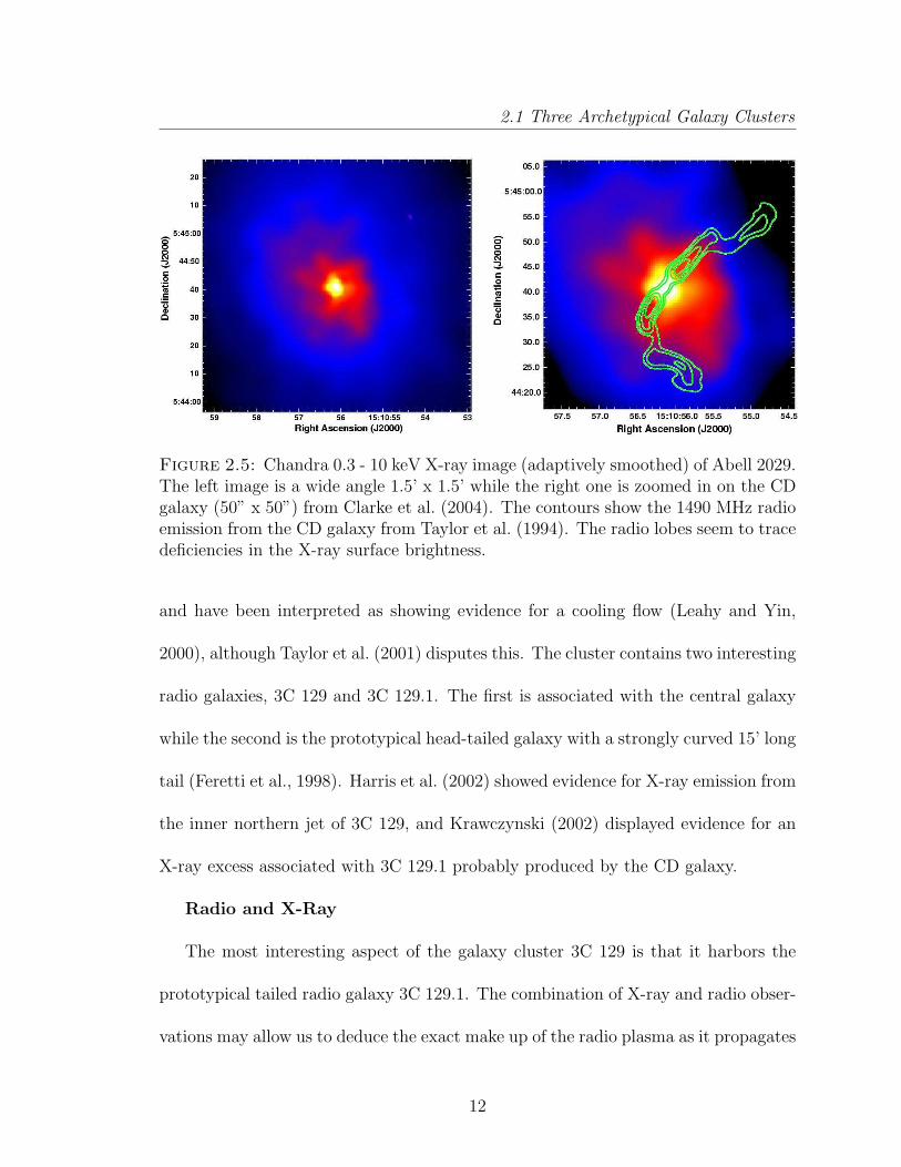
Figure 2.5: Chandra 0.3 - 10 keV X-ray image (adaptively smoothed) of Abell 2029.The left image is a wide angle 1.5’ x 1.5’ while the right one is zoomed in on the CDgalaxy (50” x 50”) from Clarke et al. (2004). The contours show the 1490 MHz radioemission from the CD galaxy from Taylor et al. (1994). The radio lobes seem to tracedeficiencies in the X-ray surface brightness.
and have been interpreted as showing evidence for a cooling flow (Leahy and Yin,
2000), although Taylor et al. (2001) disputes this. The cluster contains two interesting
radio galaxies, 3C 129 and 3C 129.1. The first is associated with the central galaxy
while the second is the prototypical head-tailed galaxy with a strongly curved 15’ long
tail (Feretti et al., 1998). Harris et al. (2002) showed evidence for X-ray emission from
the inner northern jet of 3C 129, and Krawczynski (2002) displayed evidence for an
X-ray excess associated with 3C 129.1 probably produced by the CD galaxy.
Radio and X-Ray
The most interesting aspect of the galaxy cluster 3C 129 is that it harbors the
prototypical tailed radio galaxy 3C 129.1. The combination of X-ray and radio obser-
vations may allow us to deduce the exact make up of the radio plasma as it propagates
12

2.2 The X-Ray and Gamma-Ray Astrophysics of Galaxy Clusters
through the ICM. Since the X-ray data informs us about the temperature, chemical
composition, density and pressure of the ICM we can study the pressure balance be-
tween the radio plasma and the thermal gas in great detail. A pressure balance study
based on various radio maps of the radio galaxy 3C 129 and on the Chandra observa-
tion of the cluster, indicates an apparent pressure mismatch between the pressure of
the radio tail and the adjacent ICM. This mismatch is indicative for ”dark” pressure
components (like relativistic protons or magnetic field) that carry additional pressure
of the radio plasma. The detection of a cavity associated with the radio tail would
further constrain the composition of the radio tail plasma. This is one of the main
objectives of the XMM-Newton observations described further below.
2.2 The X-Ray and Gamma-Ray Astrophysics of
Galaxy Clusters
One of the most significant features of the ICM is that it emits mainly X-rays. This
led to a late understanding of the ICM and clusters because the first high sensitivity
X-ray observatories were launched in the late 1960s. As a whole object, clusters have
a typical luminosity of 1044 erg/sec, which corresponds to a temperature of 107 Kelvin
(see Section 2.2.1).
The first cluster was detected in X-rays by Byram et al. (1966) using the Aer-
obee observatory. This caused much excitement in the astrophysics community and
there was a rush of observing and developing of newer and more modern equipment
13

2.2 The X-Ray and Gamma-Ray Astrophysics of Galaxy Clusters
to better resolve clusters and consequently provide data to better explain the emis-
sion mechanism. In 1976, Iron lines were first resolved (Mitchell et al., 1976) and
this placed the theory of thermal emission via bremsstrahlung on firm experimental
ground. The most significant step forward in the resulting studies of clusters was the
development of improved resolution observatories such as Chandra and ROSAT.
This section will focus on the general theoretical ideas explaining the X-ray emis-
sion from clusters. It will begin with thermal bremsstrahlung (the main emission
mechanism in clusters) emission. From there, various VHE emission processes will be
discussed that might be observable from clusters. Finally, the astrophysics specific to
clusters will be presented.
2.2.1 Thermal Bremsstrahlung
When clusters were first observed in X-rays there were several different theories as
to the origin of this radiation. Among those included where thermal bremsstrahlung
emission, a population of individual sources and inverse Compton scattering. Of these
three, thermal bremsstrahlung is the only valid model used to describe clusters today.
There are several reasons to assume that the overall X-ray emission from clusters is
thermal in nature and very few arguments for the other two theories. In reference to
individual sources, one would expect a granularity of the cluster emission, which is
not observed and would not expect to see line emissions, which is observed. As for
inverse Compton emission, there should be a correlation between the radio emissions
and the X-ray emissions; the spectra should behave like a power law and you would
14
2.2 The X-Ray and Gamma-Ray Astrophysics of Galaxy Clusters
not see line emissions. None of these conditions are met for clusters. Conversely, one
would expect non-granularity, no x-ray/radio correlations, an exponential spectrum
and line emissions if the cluster were emitting thermally (Sarazin, 1988).
Thermal bremsstrahlung is the radiation associated with accelerating electrons in
the electrostatic fields of atoms and ions. The standard model involves a large ball of
optically thin hot plasma consisting of atoms, ions and electrons populating the region
between the galaxies in the cluster much like there is a plasma in the regions between
stars in our own galaxy. Clusters emit thermally via bremsstrahlung emission and
not black body emission because the ICM is optically thin.
The derivation of bremsstrahlung involves starting with the emission of brak-
ing/acceleration radiation of an electron as it interacts with the nucleus of an atom.
This result can then be used to calculate the total emission from a plasma inter-
acting with a gas of ions (for a detailed calculation see Longair (1992) or Jackson
(1999)). The following outlines the derivation found in Longair, which indicates that
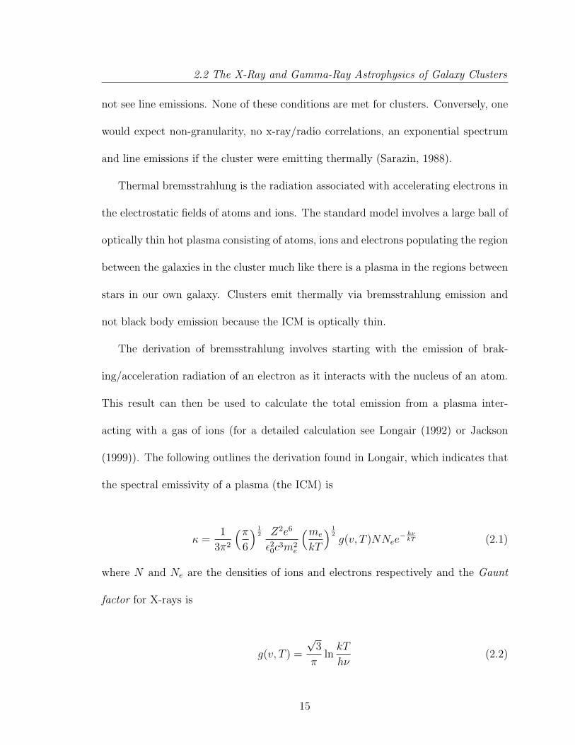
the spectral emissivity of a plasma (the ICM) is
κ =1
3π2
(π
6
) 12 Z2e6
ε20c
3m2e
(me
kT
) 12g(v, T )NNee
− hνkT (2.1)
where N and Ne are the densities of ions and electrons respectively and the Gaunt
factor for X-rays is
g(v, T ) =
√3
πln
kT
hν(2.2)
15
2.2 The X-Ray and Gamma-Ray Astrophysics of Galaxy Clusters
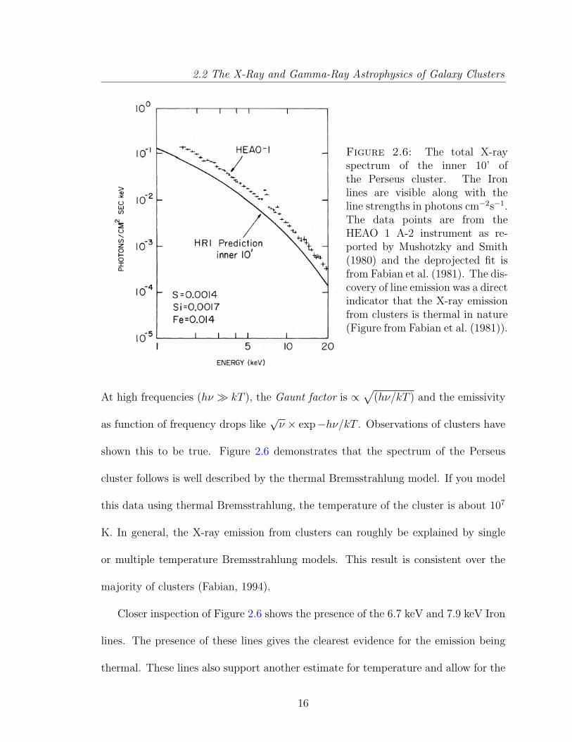
Figure 2.6: The total X-rayspectrum of the inner 10’ ofthe Perseus cluster. The Ironlines are visible along with theline strengths in photons cm−2s−1.The data points are from theHEAO 1 A-2 instrument as re-ported by Mushotzky and Smith(1980) and the deprojected fit isfrom Fabian et al. (1981). The dis-covery of line emission was a directindicator that the X-ray emissionfrom clusters is thermal in nature(Figure from Fabian et al. (1981)).
At high frequencies (hν kT ), the Gaunt factor is ∝√
(hν/kT ) and the emissivity
as function of frequency drops like√
ν × exp−hν/kT . Observations of clusters have
shown this to be true. Figure 2.6 demonstrates that the spectrum of the Perseus
cluster follows is well described by the thermal Bremsstrahlung model. If you model
this data using thermal Bremsstrahlung, the temperature of the cluster is about 107
K. In general, the X-ray emission from clusters can roughly be explained by single
or multiple temperature Bremsstrahlung models. This result is consistent over the
majority of clusters (Fabian, 1994).
Closer inspection of Figure 2.6 shows the presence of the 6.7 keV and 7.9 keV Iron
lines. The presence of these lines gives the clearest evidence for the emission being
thermal. These lines also support another estimate for temperature and allow for the
16
2.2 The X-Ray and Gamma-Ray Astrophysics of Galaxy Clusters
measuring of the ICM mass and the total mass of the cluster. There are also lines
showing the presence of significant amounts of other elements with atomic number
up to Iron. The similarity of the abundances (approximately solar) of these metals
among multiple clusters suggests a similar evolutionary history for all clusters. In
other words, clusters appear to have formed through the same type of evolutionary
process independent of their present dynamical state. The nearly solar abundance of
these metals in the ICM establishes that the ICM is at least partly processed matter
from stars and cannot be wholly primordial matter, since primordial matter would
be mainly composed of hydrogen and some helium.
2.2.2 Thermal and Non-Thermal Particles in Clusters
There are two distinct populations of particles within galaxy clusters: the thermal
(ICM) and non-thermal (CRp, CRe and AGN jets). While the thermal particles
interact with each other frequently and establish a thermal (Maxwellian) distribution
of velocities, higher energy particles interact little with the thermal plasma. The
reason for this behavior can be understood with the help of the Bethe-Bloch formula:
− dE
dx=
z2e4Ne
4πε20mev2
[ln
(2γ2mev
2
I
)− v2
c2
](2.3)
The formula in Equation 2.3 shows that the energy loss rate depends only upon
the velocity and charge of the particles. At the lower energies (approximately non-
relativistic) the ionization loss is proportional to v−2 or E−1, but at higher energies the
rate is only logarithmically dependent on E. The relative energy loss rate, dEdt
/E, is
17
2.2 The X-Ray and Gamma-Ray Astrophysics of Galaxy Clusters
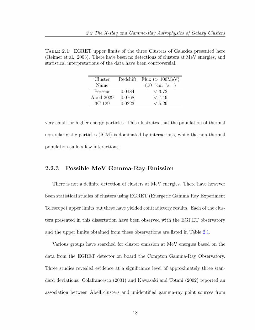
Table 2.1: EGRET upper limits of the three Clusters of Galaxies presented here(Reimer et al., 2003). There have been no detections of clusters at MeV energies, andstatistical interpretations of the data have been controversial.
Cluster Redshift Flux (> 100MeV)Name (10−8cm−2s−1)
Perseus 0.0184 < 3.72Abell 2029 0.0768 < 7.49
3C 129 0.0223 < 5.29
very small for higher energy particles. This illustrates that the population of thermal
non-relativistic particles (ICM) is dominated by interactions, while the non-thermal
population suffers few interactions.
2.2.3 Possible MeV Gamma-Ray Emission
There is not a definite detection of clusters at MeV energies. There have however
been statistical studies of clusters using EGRET (Energetic Gamma Ray Experiment
Telescope) upper limits but these have yielded contradictory results. Each of the clus-
ters presented in this dissertation have been observed with the EGRET observatory
and the upper limits obtained from these observations are listed in Table 2.1.
Various groups have searched for cluster emission at MeV energies based on the
data from the EGRET detector on board the Compton Gamma-Ray Observatory.
Three studies revealed evidence at a significance level of approximately three stan-
dard deviations: Colafrancesco (2001) and Kawasaki and Totani (2002) reported an
association between Abell clusters and unidentified gamma-ray point sources from
18

2.2 The X-Ray and Gamma-Ray Astrophysics of Galaxy Clusters
the third catalog of the EGRET experiment; Scharf and Mukherjee (2002) found
gamma-ray emission from Abell clusters by stacking the EGRET data of 447 galaxy
clusters. Reimer et al. (2003) analyzed data from 58 galaxy clusters and did not con-
firm a detection. The upper limit provided by Reimer is inconsistent with the mean
flux reported by Scharf and Mukherjee (2002). In the TeV energy range, Fegan et al.
(2005) reported marginal evidence for emission from Abell 1758 in the field of view
of 3EG J1337 +5029.
2.2.4 VHE Gamma-Ray Emission Mechanisms
CRe lose their energy by emitting synchrotron, Bremsstrahlung, and inverse Comp-
ton emission on much shorter time scales. For ICM magnetic fields on the order of
B ' 1µG, synchrotron and inverse Compton emission losses alone cool CRe of energy
E = 1 TeV on a timescale
τs =
(4
3σT c
B′2
8πmec2γe
)−1
(2.4)
where σT is the Thomson cross section, B′ =√
B2 + B2CMB and
BCMB = 3.25(1 + z)2µG; for the clusters considered here, z 1 and τs ≈ 106 years.
The short life-time of TeV electrons implies that they do not accumulate over the life
time of the cluster. If we observed Inverse Compton TeV gamma rays from a cluster,
it would come from electrons that were accelerated at most a few million years before
they emitted the radiation.
There is good observational evidence for nonthermal electrons in galaxy clus-
19
2.2 The X-Ray and Gamma-Ray Astrophysics of Galaxy Clusters
ters. For a number of clusters, diffuse synchrotron radio halos and/or radio relic
sources have been detected (Giovannini et al., 1993, 1999; Giovannini and Feretti,
2000; Kempner and Sarazin, 2001; Feretti, 2003). For some clusters, an excess of
Extreme Ultra-Violet (EUV) and/or hard X-ray radiation over that expected from
the thermal X-ray emitting ICM has been observed (Bowyer and Berghofer, 1998;
Lieu et al., 1999; Rephaeli et al., 1999; Fusco-Femiano et al., 2004). The excess radi-
ation originates most likely as inverse Compton emission from CRe scattering cosmic
microwave background photons (Lieu et al., 1996; Enßlin and Biermann, 1998; Blasi
and Colafrancesco, 1999; Fusco-Femiano et al., 1999).
The detection of gamma-ray emission from galaxy clusters would make it possi-
ble to measure the energy density of non-thermal particles. The density and energy
density of the thermal ICM can be derived from imaging-spectroscopy observations
made with such satellites as Chandra and XMM-Newton (Markevitch et al., 1998;
Krawczynski, 2002; Donahue et al., 2004). The density and energy spectra of the
non-thermal protons could be computed from the detected gamma-ray emission once
the density of the thermal ICM is known (Pfrommer and Enßlin, 2004). Gamma
rays can originate as inverse Compton and Bremsstrahlung emission from CRe and
as π0 → γγ emission from hadronic interactions of CRp with thermal target material.
Successful measurements of the gamma-ray fluxes from several galaxy clusters would
allow the correlation of the CRp luminosity with cluster mass, temperature, and red-
shift, and provide conclusions about how the clusters grew. Assuming CRp contribute
noticeably to the pressure of the ICM, the measurements of the CRp energy density
20
2.2 The X-Ray and Gamma-Ray Astrophysics of Galaxy Clusters
would allow improvement on the estimates of the cluster mass based on X-ray data,
and thus improve estimates of the universal baryon fraction. If CR provide pressure
support to the ICM, they would inhibit star formation to some extent as they do not
cool radiatively like the thermal X-ray emitting gas. However, if CRp give less pres-
sure support than the ICM they might accelerate star formation. Furthermore, low
energy cosmic ray ions might provide a source of heating the thermal gas (Rephaeli,
1977).
In addition to a CR origin, annihilating dark matter may also emit gamma rays.
The intensity of the radiation depends on the nature of dark matter, the annihilation
cross sections, and the dark matter density profile close to the core of the cluster
(Bergstrom et al., 1998). While MeV observations are ideally suited for detecting the
emission from the bulk of the non-thermal particles, TeV gamma-ray observations
of cluster energy spectra and radial emission profiles would disentangle the various
components that contribute to the emission.
The search for TeV emission from clusters described in Chapter 5 assumes that
the high energy (HE) surface brightness mimics the X-ray surface brightness, and
focuses on the detection of gamma rays from within 0.8 degrees from the cluster cen-
ter. There are several possibilities connecting the thermal and non-thermal particles
within clusters. From general considerations, Volk and Atoyan (1999) assume that
the non-thermal particles carry a certain fraction of the energy density of the ICM.
One of the aims of VHE astronomy is to constrain this fraction. The CRp energy
density in the Interstellar Medium (ISM) of the Milky Way galaxy is comparable to
21
2.2 The X-Ray and Gamma-Ray Astrophysics of Galaxy Clusters
the energy density of the thermal ISM, the energy density of the interstellar magnetic
field and the energy density of star light. If non-thermal particles in clusters indeed
carry a certain fraction of the energy density of the ICM, the HE surface brightness
would mimic that of the thermal X-ray emission. A differing argument is that pow-
erful cluster members (i.e. radio sources) are the dominant source of non-thermal
particles in the ICM. In this circumstance we would expect that CRp accumulate at
the cluster cores where usually the most powerful radio galaxies are found (Pfrommer
and Enßlin, 2004). Ryu et al. (2003) and Kang and Jones (2005) performed numerical
calculations to estimate the energy density of CRp by large scale structure formation
shocks. The simulations indicate that strong shocks form preferentially in the cluster
periphery. Accordingly, most CRp would be accelerated in the outskirts of the clus-
ters and would only slowly be transported to the cluster core by bulk plasma motion
following cluster merger for example. In conclusion, the CRp distribution in galaxy
clusters is uncertain as long as we have not mapped them in the light of HE photons.
However, independent of the lateral profile of CRp acceleration, the emission profile
is expected to be centrally peaked, as the HE emission stems from inelastic collisions
of the CRps with the centrally peaked thermal target material.
2.2.5 Extragalactic Extinction
Unfortunately, the Universe is rather opaque at gamma-ray energies above 30
GeV. The primary process that removes high energy gamma rays of energy E from
remote objects is absorption via γE + γε → e+ + e− as they move through the low
22
2.2 The X-Ray and Gamma-Ray Astrophysics of Galaxy Clusters
energy photons of the extragalactic background light (EBL). When the photons are
in the VHE gamma-ray region they then interact as described with photons from the
Infrared Background and arrive with a spectrum that has been modified by the EBL
absorption. There have been notable advances in measuring the EBL and several
attempts to estimate its effect on gamma-ray emission.
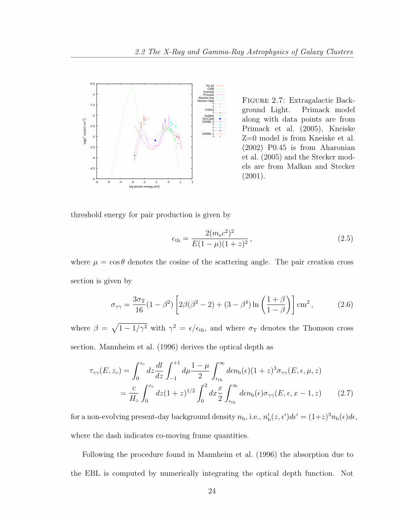
Figure 2.7 compares several different EBL models along with recent measurements
of the EBL over a large energy range. None of the models are fully analytical. The
Primack model (Primack et al., 2005) calculated the emission by using an evolving
galaxy population model using semi-analytical procedures, taking into account the
effects of dust which obscures the IR and re-radiates the absorption. The model by
Malkan and Stecker (2001) (called Stecker here) assumed that the the dependence on
galactic spectra is the same for all redshifts and added a simple luminosity evolution
back to a redshift of 2. Kneiske et al. (2002) based their model directly on the
observations and used a minimal set of assumptions to pinpoint the basic physics
involved. Their model is very similar to the Stecker model (Malkan and Stecker,
2001), but specifically addressed the redshift evolution of the EBL as well as re-
radiation. The P0.45 model from Aharonian et al. (2005) is a simple interpolation
of the EBL data and is consistent with the recent detection of blazars with hard
gamma-ray energy spectra at redshifts of 0.18 with the H.E.S.S. experiment.
Given a model for the EBL the optical depth can be computed as follows: the
23
2.2 The X-Ray and Gamma-Ray Astrophysics of Galaxy Clusters
-5
-4.5
-4
-3.5
-3
-2.5
-2
-1.5
-1
-0.5
-6 -5 -4 -3 -2 -1 0 1 2
log[
ε2 n(ε
)/eV
cm
-3]
log photon energy [eV]
P0.45CMB
KneiskePrimack
Stecker-lowStecker-high
??
FIRAS?
HubbleISOCAMDIRBE 2
???
DIRBE 1?
Figure 2.7: Extragalactic Back-ground Light. Primack modelalong with data points are fromPrimack et al. (2005), KneiskeZ=0 model is from Kneiske et al.(2002) P0.45 is from Aharonianet al. (2005) and the Stecker mod-els are from Malkan and Stecker(2001).
threshold energy for pair production is given by
εth =2(mec
2)2
E(1− µ)(1 + z)2, (2.5)
where µ = cos θ denotes the cosine of the scattering angle. The pair creation cross
section is given by
σγγ =3σT
16(1− β2)
[2β(β2 − 2) + (3− β4) ln
(1 + β
1− β
)]cm2 , (2.6)
where β =√
1− 1/γ2 with γ2 = ε/εth, and where σT denotes the Thomson cross
section. Mannheim et al. (1996) derives the optical depth as
τγγ(E, z) =
∫ z
0
dzdl
dz
∫ +1
−1
dµ1− µ
2
∫ ∞
εth
dεnb(ε)(1 + z)3σγγ(E, ε, µ, z)
=c
H
∫ z
0
dz(1 + z)1/2
∫ 2
0
dxx
2
∫ ∞
εth
dεnb(ε)σγγ(E, ε, x− 1, z) (2.7)
for a non-evolving present-day background density nb, i.e., n′b(z, ε′)dε′ = (1+z)3nb(ε)dε,
where the dash indicates co-moving frame quantities.
Following the procedure found in Mannheim et al. (1996) the absorption due to
the EBL is computed by numerically integrating the optical depth function. Not
24
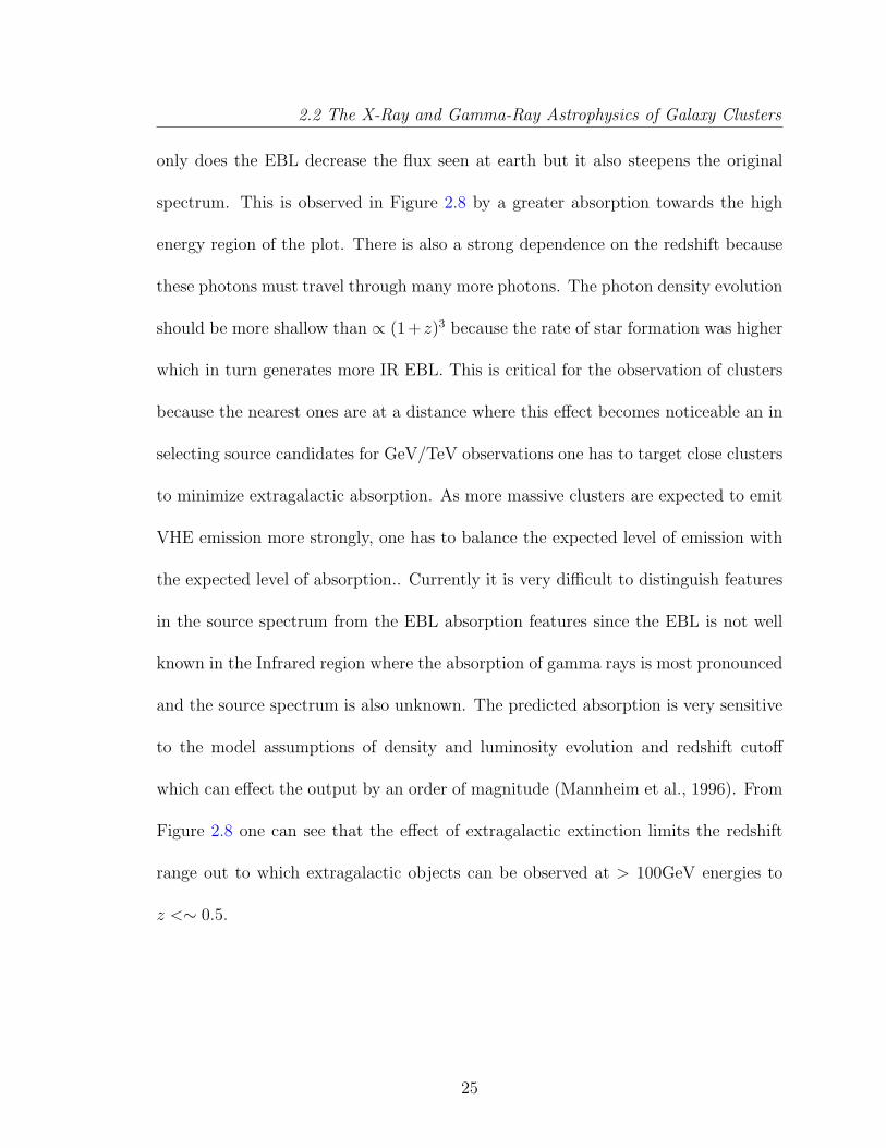
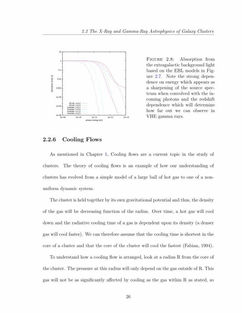
2.2 The X-Ray and Gamma-Ray Astrophysics of Galaxy Clusters
only does the EBL decrease the flux seen at earth but it also steepens the original
spectrum. This is observed in Figure 2.8 by a greater absorption towards the high
energy region of the plot. There is also a strong dependence on the redshift because
these photons must travel through many more photons. The photon density evolution
should be more shallow than ∝ (1+ z)3 because the rate of star formation was higher
which in turn generates more IR EBL. This is critical for the observation of clusters
because the nearest ones are at a distance where this effect becomes noticeable an in
selecting source candidates for GeV/TeV observations one has to target close clusters
to minimize extragalactic absorption. As more massive clusters are expected to emit
VHE emission more strongly, one has to balance the expected level of emission with
the expected level of absorption.. Currently it is very difficult to distinguish features
in the source spectrum from the EBL absorption features since the EBL is not well
known in the Infrared region where the absorption of gamma rays is most pronounced
and the source spectrum is also unknown. The predicted absorption is very sensitive
to the model assumptions of density and luminosity evolution and redshift cutoff
which can effect the output by an order of magnitude (Mannheim et al., 1996). From
Figure 2.8 one can see that the effect of extragalactic extinction limits the redshift
range out to which extragalactic objects can be observed at > 100GeV energies to
z <∼ 0.5.
25
2.2 The X-Ray and Gamma-Ray Astrophysics of Galaxy Clusters
1e-06
1e-05
1e-04
0.001
0.01
0.1
1
10
1e+09 1e+10 1e+11 1e+12 1e+13
abso
rptio
n [e
xp(-
τ)]
photon energy [eV]
P0.45, z=0.2P0.45, z=0.4
Kneiske, z=0.2Kneiske, z=0.4Kneiske, z=1.0Kneiske, z=2.0
Figure 2.8: Absorption fromthe extragalactic background lightbased on the EBL models in Fig-ure 2.7. Note the strong depen-dence on energy which appears asa sharpening of the source spec-trum when convolved with the in-coming photons and the redshiftdependence which will determinehow far out we can observe inVHE gamma rays.
2.2.6 Cooling Flows
As mentioned in Chapter 1, Cooling flows are a current topic in the study of
clusters. The theory of cooling flows is an example of how our understanding of
clusters has evolved from a simple model of a large ball of hot gas to one of a non-
uniform dynamic system.
The cluster is held together by its own gravitational potential and thus, the density
of the gas will be decreasing function of the radius. Over time, a hot gas will cool
down and the radiative cooling time of a gas is dependent upon its density (a denser
gas will cool faster). We can therefore assume that the cooling time is shortest in the
core of a cluster and that the core of the cluster will cool the fastest (Fabian, 1994).
To understand how a cooling flow is arranged, look at a radius R from the core of
the cluster. The pressure at this radius will only depend on the gas outside of R. This
gas will not be as significantly affected by cooling as the gas within R as stated, so
26
2.2 The X-Ray and Gamma-Ray Astrophysics of Galaxy Clusters
there will be a temperature gradient across R. The pressure slightly above and below
R will be practically the same and the volume will also remain roughly constant but
the temperature will definitely be different due to the faster cooling inside of R. To
maintain the pressure and volume at R, the density must rise to compensate for this
decrease in temperature. The only way for this to happen is for matter to fall below
R. This is the essence of a cooling flow, a flow of matter into the core of the cluster
due to a temperature gradient within the cluster (Fabian, 1994).
An example of a cooling flow can be best displayed by comparing the surface
brightness of a non-cooling flow cluster like Coma to a cooling flow cluster like Cen-
taurus. The surface brightness of the non-cooling type will be rather flat with radius
indicating a rather constant density throughout the ICM, while the cooling type will
continue to rise inversely with radius all the way to the core (indicative of a dense
core). The radial dependence of the temperature can be determined by examining
the spectral data from the cluster. For cooling flow clusters the temperature should
decrease as you travel towards the core and this has partially been observed.
Observing the luminosity within the cooling region (i.e. where the cooling rate
is significantly small) and with the assumption that this luminosity is only due to
the thermal energy of the gas and the PdV work done on the gas as it falls into
the potential well of the cluster in the cooling flow, then L = 5M2µm
kT where M , µ
and m are the mass deposition rate, the mean molecular mass, and the proton mass
respectively. With the luminosity of the cooling region known the mass deposition
rate can be determined from this equation. The mass deposition rate, measured in
27
2.2 The X-Ray and Gamma-Ray Astrophysics of Galaxy Clusters
solar masses per year, ranges from 0 to > 500 with 50 - 100 being typical values
(Fabian, 1994).
As cool ICM is deposited into the center of the cluster, one would expect the
formation of either cold clouds or gravitational collapse into star formation. However,
observations with Chandra and XMM-Newton did not find cold gas with kBT < 1keV
(Peterson et al., 2004). The predicted star formation regions have also not been found.
There are many models to explain the failure of the cooling flow model including the
heating of the ICM by central AGN or a higher thermal conductivity of the ICM
preventing the rapid cooling of the center (Donahue and Voit, 2004; Blanton, 2004).
The search for evidence with respect to these theories is a continuing field of study.
Overall, there are numerous phenomenon available for study in clusters. The
ICM radiates mainly in the X-ray via thermal Bremsstrahlung emission which allows
for the measurement of composition and temperature of the cluster and the spatial
distribution of dark matter. Based on the current understanding of clusters, one
would expect to find evidence of cool, dense cores but the lack of this evidence of
such features has led to the search for a type of heating at the core. There is evidence
for non-thermal emission from clusters due to the observations of radio galaxies and
AGN within clusters. Several studies have been made to look for MeV emission from
clusters but the results remain inconclusive and more observations at higher energies
are needed. At the highest of energies, extragalactic extinction becomes relevant and
one can only observe the closest most massive clusters.
28
Chapter 3
X-Ray and Gamma-Ray
Observatories
The data presented in this dissertation were collected with several different ob-
servatories including the orbiting observatories, XMM-Newton and Chandra, and the
ground-based Whipple 10m Gamma-ray Telescope in Amado, Arizona. In this chap-
ter I describe the instruments and techniques used to detect photons in each of these
experiments.
3.1 X-Ray Observatories
In the high energy range of 100 eV to several keV, observations are best achieved
in space. In this range, the atmosphere absorbs the radiation and reasonably-sized
detectors can register a sufficient number of photons to warrant sensitive observa-
29

3.1 X-Ray Observatories
tions. Modern missions use solid state detectors to detect the photons and there are
currently two major observatories, Chandra and XMM-Newton. These instruments,
while using the same basic detector technique, are very different in terms of their
angular resolution and effective area. Chandra has approximately forty times the
angular resolution of XMM (X-ray Multi Mirror) while XMM has a much larger (6x)
detection area.
3.1.1 Solid State Detectors
Both Chandra and XMM-Newton use Silicon-based Charged Coupled Devices
(CCDs) to detect X-ray photons from astrophysical objects. A CCD is an array of
MOS diodes, except in the case of the PN detectors on board the XMM-Newton
detector (see Section 3.1.2). When a photon interacts with the substrate material
(usually p-type Silicon), it creates a number of electron-hole pairs dependent on the
energy of the original photon. The initial MOS diode is biased in such a way that
the charge is contained within the single MOS detector. On readout, the charge is
transferred along each individual array element (or pixel) towards a readout element
where it is then digitized. The importance in terms of high energy astrophysics is
that the response of the detector can be tuned to the energy region of interest. These
types of detectors can be very compact with the FET amplifier built on the chips
themselves. The technology has progressed to minimize the cost and provide very
mature instruments.
30
3.1 X-Ray Observatories
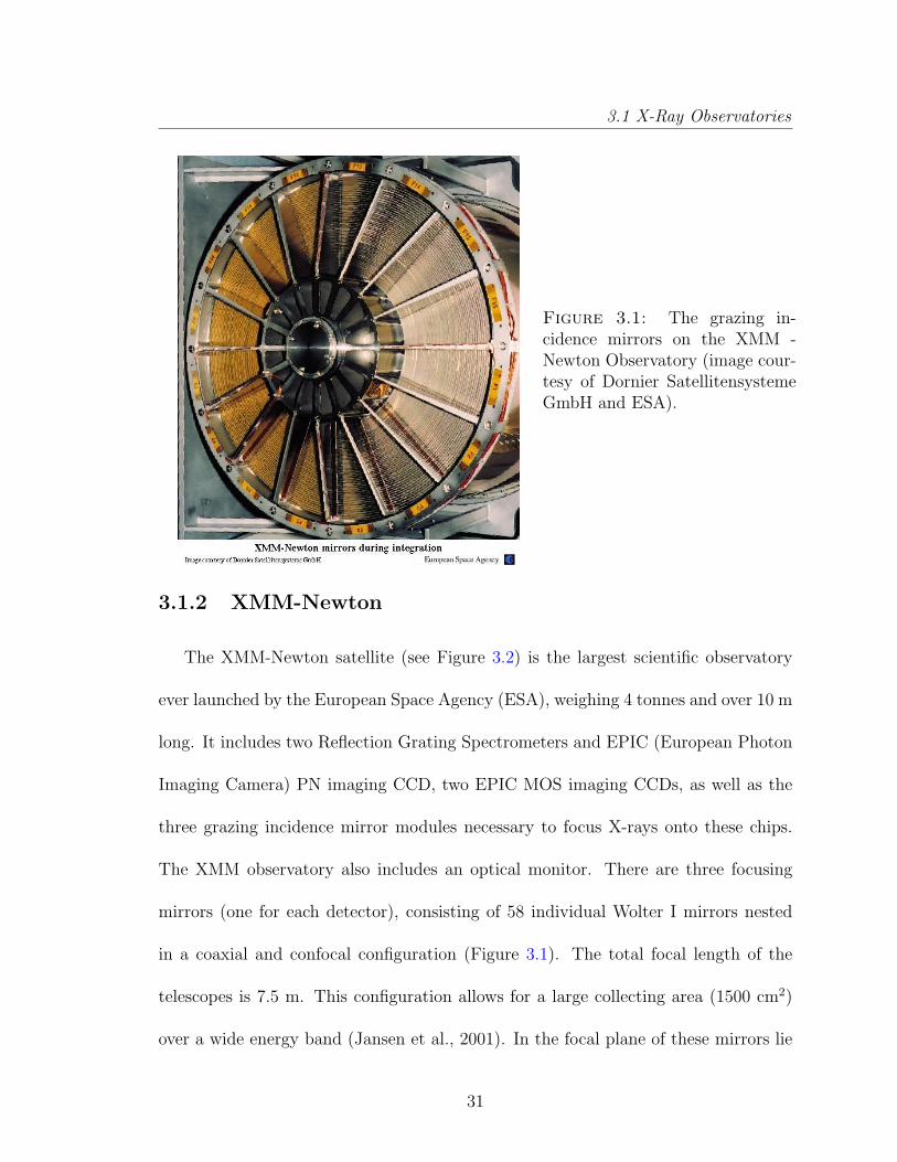
Figure 3.1: The grazing in-cidence mirrors on the XMM -Newton Observatory (image cour-tesy of Dornier SatellitensystemeGmbH and ESA).
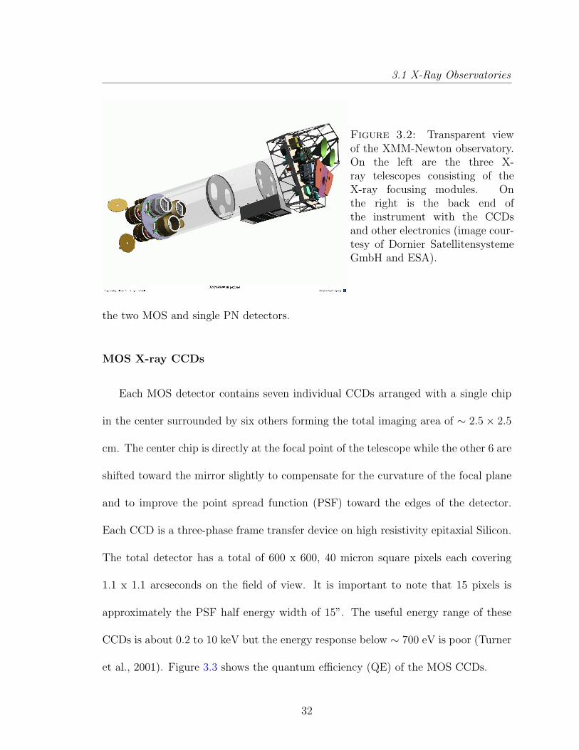
3.1.2 XMM-Newton
The XMM-Newton satellite (see Figure 3.2) is the largest scientific observatory
ever launched by the European Space Agency (ESA), weighing 4 tonnes and over 10 m
long. It includes two Reflection Grating Spectrometers and EPIC (European Photon
Imaging Camera) PN imaging CCD, two EPIC MOS imaging CCDs, as well as the
three grazing incidence mirror modules necessary to focus X-rays onto these chips.
The XMM observatory also includes an optical monitor. There are three focusing
mirrors (one for each detector), consisting of 58 individual Wolter I mirrors nested
in a coaxial and confocal configuration (Figure 3.1). The total focal length of the
telescopes is 7.5 m. This configuration allows for a large collecting area (1500 cm2)
over a wide energy band (Jansen et al., 2001). In the focal plane of these mirrors lie
31
3.1 X-Ray Observatories
Figure 3.2: Transparent viewof the XMM-Newton observatory.On the left are the three X-ray telescopes consisting of theX-ray focusing modules. Onthe right is the back end ofthe instrument with the CCDsand other electronics (image cour-tesy of Dornier SatellitensystemeGmbH and ESA).
the two MOS and single PN detectors.
MOS X-ray CCDs
Each MOS detector contains seven individual CCDs arranged with a single chip
in the center surrounded by six others forming the total imaging area of ∼ 2.5× 2.5
cm. The center chip is directly at the focal point of the telescope while the other 6 are
shifted toward the mirror slightly to compensate for the curvature of the focal plane
and to improve the point spread function (PSF) toward the edges of the detector.
Each CCD is a three-phase frame transfer device on high resistivity epitaxial Silicon.
The total detector has a total of 600 x 600, 40 micron square pixels each covering
1.1 x 1.1 arcseconds on the field of view. It is important to note that 15 pixels is
approximately the PSF half energy width of 15”. The useful energy range of these
CCDs is about 0.2 to 10 keV but the energy response below ∼ 700 eV is poor (Turner
et al., 2001). Figure 3.3 shows the quantum efficiency (QE) of the MOS CCDs.
32

3.1 X-Ray Observatories
Figure 3.3: The X-ray quantumefficiency of the EPIC MOS CCDsbased on ground based calibra-tions using the Orsay synchrotron(Pigot et al., 1999; Trifoglio et al.,1998) and celestrial source mea-surements since launch (Turneret al., 2001). These data are use-ful in determining the effective en-ergy region in which to observe anobject.
The MOS imagers are behind a filter wheel containing four possible choices of
filtering (in addition to the light and UV blocking filters). Two of the filters are
thin films made of 1600 A poly-imide with 400 A aluminum on one side. There is
also a medium filter with the same substrate but 800 A of aluminum and a thick
filter with 3300 A of Polypropylene with 1100 A of aluminum and 450 A of tin. The
choice of filter is determined by the strength of the source. There are also open and
closed filters available. The open mode is only used for very dim fields of view while
the closed position is used during periods of high proton fluxes and is also useful for
particle background measurements (Turner et al., 2001).
PN X-ray CCDs
The other CCD residing in the focal plane of the X-ray telescope is a type of
Silicon drift detector. These are fully depleted CCDs with a thickness of 300µm
which differs from the MOS detectors and the CCDs used on Chandra. The leading
benefit from this type of detector is a high detection efficiency above 5 keV. The pixel
33

3.1 X-Ray Observatories
Figure 3.4: The X-ray quantumefficiency of the EPIC PN CCDbased on ground based calibra-tions using the Orsay synchrotron(Pigot et al., 1999; Trifoglio et al.,1998) and celestrial source mea-surements since launch (Struderet al., 2001). These data are use-ful in determining the effective en-ergy region in which to observean object. The QE of the PN ismuch flatter over the full energyrange than the MOS detectors onboard XMM, which decreases sub-stantially above 5 keV.
size can be tailored to the X-ray optics and results in a combined angular resolution
of 3.3 arcsecond. The full detector is made up of twelve individual chips arranged in
a rectangular grid with a sensitive area of 36cm2. The detector is cooled to −90C
which provides a leakage current less than 0.1 electrons per pixel over a readout cycle
of 73 ms. The quantum efficiency of the PN detector is flatter over the full energy
range than the MOS detector and can be seen in Figure 3.4 (Struder et al., 2001).
Optical
The addition of the optical and UV imagers on board the XMM-Newton observa-
tory allows simultaneous observations of objects over a very broad energy range. The
coverage extends the range of the observatory between 170 to 650 nm and is focused
on the central 17 arcmin of the X-ray FOV. In addition to being able to image ob-
jects with great sensitivity due to low background using several on-board filters, the
34
3.1 X-Ray Observatories
instrument can also perform spectroscopy using a grism. At the focal plane of this
instrument is a microchannelplate-intensified CCD (Mason et al., 2001).
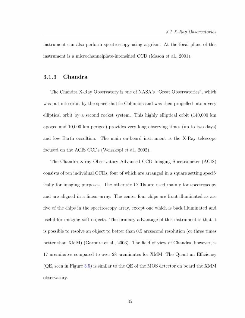
3.1.3 Chandra
The Chandra X-Ray Observatory is one of NASA’s “Great Observatories”, which
was put into orbit by the space shuttle Columbia and was then propelled into a very
elliptical orbit by a second rocket system. This highly elliptical orbit (140,000 km
apogee and 10,000 km perigee) provides very long observing times (up to two days)
and low Earth occultion. The main on-board instrument is the X-Ray telescope
focused on the ACIS CCDs (Weisskopf et al., 2002).
The Chandra X-ray Observatory Advanced CCD Imaging Spectrometer (ACIS)
consists of ten individual CCDs, four of which are arranged in a square setting specif-
ically for imaging purposes. The other six CCDs are used mainly for spectroscopy
and are aligned in a linear array. The center four chips are front illuminated as are
five of the chips in the spectroscopy array, except one which is back illuminated and
useful for imaging soft objects. The primary advantage of this instrument is that it
is possible to resolve an object to better than 0.5 arcsecond resolution (or three times
better than XMM) (Garmire et al., 2003). The field of view of Chandra, however, is
17 arcminutes compared to over 28 arcminutes for XMM. The Quantum Efficiency
(QE, seen in Figure 3.5) is similar to the QE of the MOS detector on board the XMM
observatory.
35

3.2 The Whipple Gamma-Ray Observatory
Figure 3.5: The X-ray quantumefficiency of the ASIC CCDs onthe Chandra X-Ray observatory.Nine of the detectors are front il-luminated (FI) and one is back il-luminated (BI), useful for imagingsoft objects (Garmire et al., 2003).
3.2 The Whipple Gamma-Ray Observatory
Above 10 eV our atmosphere is opaque, and to detect radiation from astronomical
sources at energies above this we must either use space-based platforms or develop
alternate techniques. Due to the low number of photons at TeV energies, the size of
space based observatories would be prohibitively large in this energy range. Over the
past forty years, scientists from Ireland, the U.K., the U.S.A., and Germany developed
the atmospheric Cherenkov technique to detect the highest energy photons from the
ground using the atmosphere as a detector medium. Astrophysicists continued to
refine this method leading to the definite detection (20 sigma) of the Crab Nebula in
1986 by the Whipple 10m Imaging Atmospheric Cherenkov Telescope (IACT) (Weekes
et al., 1989) (see Figure 3.6).
36

3.2 The Whipple Gamma-Ray Observatory
Figure 3.6: The Whipple 10mImaging Atmospheric CherenkovTelescope located on Mt. Hop-kins near Amado, AZ. This instru-ment was the first to solidly detectVHE gamma rays from the Crabnebula in 1986 (Weekes et al.,1989). Even though it is overtwenty years old, it is still a viablescientific instrument.
3.2.1 The Imaging Atmospheric Cherenkov Technique
Even though the atmosphere is opaque to photons above a certain energy, it is pos-
sible to observe objects at the highest energies by collecting the light associated with
the interaction of this radiation with the atmosphere. When a high-energy photon
enters the earth’s atmosphere, it interacts with the atoms and molecules found there
by pair-production, creating an electron and a positron. The extra energy imparted
to this pair (anything belonging to the original photon above the minimum energy)
is usually enough to propel these charged particles beyond the speed of light in the
current medium, thus producing Cherenkov radiation. Once these primary particles
have traveled approximately one radiation length, they interact with the surrounding
air molecules and emit secondary gamma-rays via bremsstrahlung emission. These
secondary gamma-rays then pair-produce and the process continues until the ioniza-
tion losses and radiation losses equilibriate and the shower gradually diminishes (see
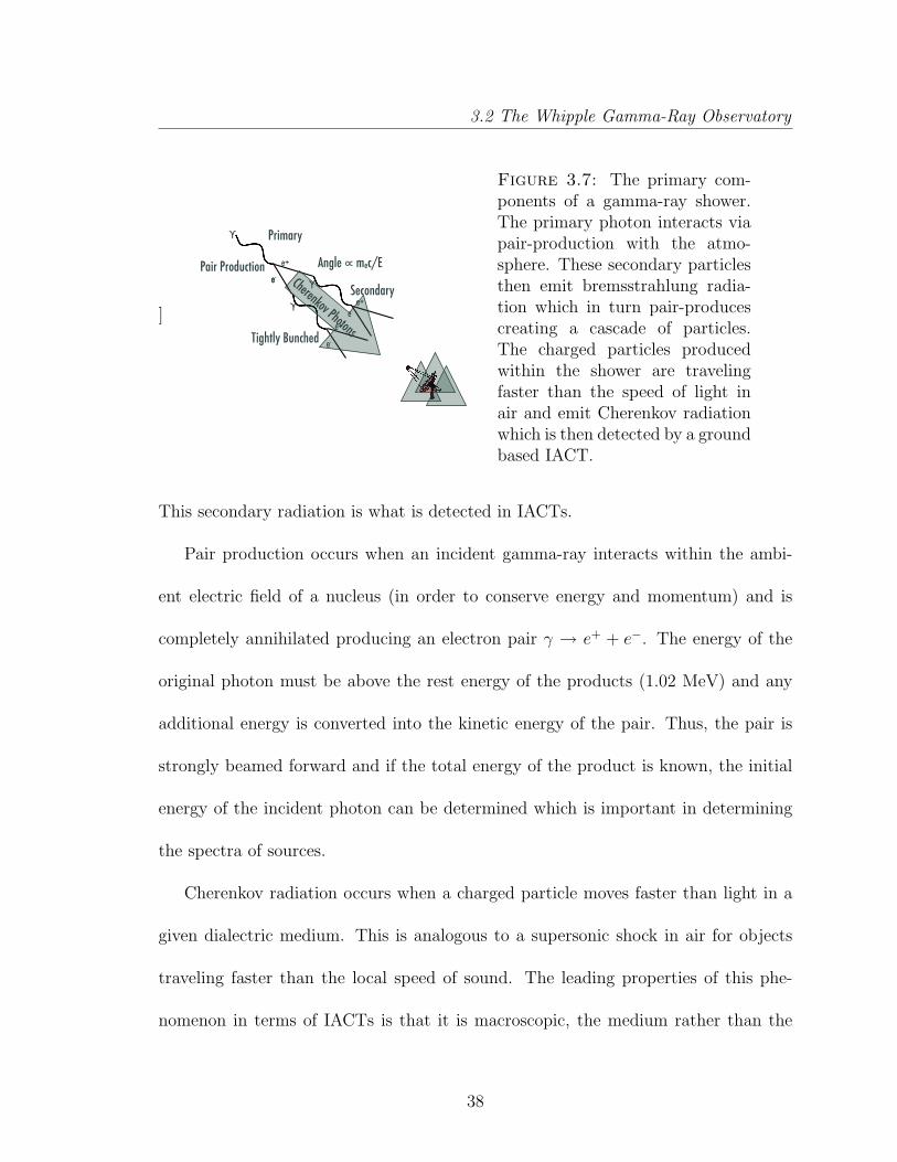
Figure 3.7 for a diagram of the process). The remarkable part of this process in terms
of IACTs is that the Cherenkov radiation is coherent and strongly beamed forward.
37
3.2 The Whipple Gamma-Ray Observatory
]
Primaryϒ
Secondaryϒ
ϒPair Production Angle ∝ mec/Ee+
e-e-
Tightly Bunched
e+
e+
e-
e-
Cherenkov Photons
Figure 3.7: The primary com-ponents of a gamma-ray shower.The primary photon interacts viapair-production with the atmo-sphere. These secondary particlesthen emit bremsstrahlung radia-tion which in turn pair-producescreating a cascade of particles.The charged particles producedwithin the shower are travelingfaster than the speed of light inair and emit Cherenkov radiationwhich is then detected by a groundbased IACT.
This secondary radiation is what is detected in IACTs.
Pair production occurs when an incident gamma-ray interacts within the ambi-
ent electric field of a nucleus (in order to conserve energy and momentum) and is
completely annihilated producing an electron pair γ → e+ + e−. The energy of the
original photon must be above the rest energy of the products (1.02 MeV) and any
additional energy is converted into the kinetic energy of the pair. Thus, the pair is
strongly beamed forward and if the total energy of the product is known, the initial
energy of the incident photon can be determined which is important in determining
the spectra of sources.
Cherenkov radiation occurs when a charged particle moves faster than light in a
given dialectric medium. This is analogous to a supersonic shock in air for objects
traveling faster than the local speed of sound. The leading properties of this phe-
nomenon in terms of IACTs is that it is macroscopic, the medium rather than the
38

3.2 The Whipple Gamma-Ray Observatory
particle is emitting, and it is low energy. Figure 3.8 demonstrates what happens when
a charged particle moves through a dialectric medium, interacting with the molecules
in the immediate vicinity, polarizing them. When the particle is non-relativistic, the
disturbance is symmetrical around the particle and there is no detectable radiation.
The situation is different when the particle is moving at a relativistic speed (i.e. when
the velocity exceeds c/n where n is the refractive index). The material cannot main-
tain and there is a resultant dipole field in the medium which produces detectable
radiation. Although there is a general canceling of the radiation due to the cylindri-
cal symmetry, there is coherent radiation in the forward direction (see Figure 3.9).
Which is detectable from the ground.
To observers on the ground, Cherenkov radiation from an electromagnetic cascade
is a glowing column of light that is dim but coherent, thus, a simple light detector
should suffice for the determination of the main quantities to be determined. From
an observational point of view, the point of origin, the energy, and the time of arrival
of the initial photon needs to be established. The point of origin can be determined
because showers are highly collimated, the energy is derived from the shower bright-
ness, and the initial photon arrival is easily concluded because the shower durations
are on the order of one nanosecond. Since the atmosphere is part of the detecting
technique, everything from temperature, pressure, and humidity will confound the
telescope yet determining these effects can be difficult or impossible. However, these
effects have been proven to be nominal by the fact that this technique works. For
example, observations of the Crab Nebula, the standard candle of TeV gamma-ray
39

3.2 The Whipple Gamma-Ray Observatory
− −+ +
−
+ −
−
−++
−− −
+− + − + + −
+
+
+
P
P
B
A
P2
1
−+
+−
P
P
B
A
− +
−+
++
+ ++
+
−
−
−−
−+
−+
++
+++
+
−
−
−−
−+
P
2
1
Figure 3.8: The effects of a charged particle moving through a dialectric medium.The figure on the left is for a non-relativistic particle while the one on the right is fora relativistic one (figure courtesy of D. Horan adapted from Jelley (1958)).
Figure 3.9: Diagram of thecoherent Cherenkov emission bya charged particle moving fasterthan light in a dialectric medium.In this figure, v is the velocityof the particle (indicated by thered arrow), β = v/c and n is therefractive index of the medium.From the geometry of the figure,one can see that cos θ = 1/nβ withθ being the emission angle of thephotons (blue arrows) (figure fromhttp://wikipedia.org).
40

3.2 The Whipple Gamma-Ray Observatory
astronomy, with different telescopes yield consistent flux levels and energy spectra.
Inclement weather is another matter and observations are only done on clear nights
which is why most telescopes are placed in dry areas with little pollution. The light
collectors needed for ACTs do not need to be precise because the size of the shower
is approximately 1.5 to 2.0 and the smallest structures are a few arcminutes in size;
assuming a resolution of a few arcminutes and a field of view of a few degrees, we
can image the shower. One of the most beneficial properties of IACTs is that the
detection area is determined by the size of the light pool, approximately 5 × 10⁴m2,
and not by the size of the telescope itself.
The Imaging Atmospheric Cherenkov Technique is background dominated and
there are several phenomena that contribute to the background. The first is the sky
brightness which can affect the energy threshold by prohibiting the detection of the
dimmest (low energy) showers. There are several ways to accommodate this; the first
is to choose light collectors (usually photo-multiplier tubes) that are most responsive
in the wavelengths where the Cherenkov emission is the brightest and where the
background light happens to be the lowest. The background lights also appear as a
constant current in the PMTs, and by setting the trigger threshold above this most of
the background can be ignored (although this still affects the energy threshold). The
second, and more troubling source of background, are charged cosmic rays which can
also produce an electromagnetic shower. There are 103 to 104 times more cosmic ray
showers than gamma-ray and while they are superficially similar there are differences
that can be used to differentiate them. Cosmic ray showers are ’messy’ in shape and
41
3.2 The Whipple Gamma-Ray Observatory
contain hadronic interactions while gamma-ray induced air showers are ’clean’ and
contain only electrons, positrons, and photons. Cosmic ray showers are incoherent,
wide, and long while gamma-ray showers are coherent, narrow, and short. Figure 3.10
displays a diagram of a cosmic ray shower compared to gamma-ray shower illustrating
the differences between the two. Aside from the night sky background and cosmic
ray showers, electrons also produce background but only at the lowest energies. The
main task during the analysis process is to determine which events are gammas and
which are hadrons.
The first generation of Atmospheric Cherenkov telescopes were non-imaging, and
could only differentiate the night sky background from shower like events. It was
not until the advent of the imaging technique that gamma hadron separation was
achieved. Instead of using a single light detector in the focal plane of the dish,
a ’camera’ (see Figure 3.12) made up multiple PMTs is used to roughly image the
shower. From the geometry of the shower, we can determine whether the shower event
was initiated by gammas or by hadrons. From simulations, we can determine that the
physics of the shower is directly responsible for the geometry of the shower, and from
these determine the cuts used to differentiate gammas and hadrons (See Section 5.1.2.
Figure 3.11 illustrates some examples of different showers look like in the camera.
As gamma-ray induced air showers are detected in many pixels of the camera, and
Cherenkov telescopes can achieve angular resolutions which are better than both the
pixel size and the optical quality of the mirrors. The energy of the primary ray
can be determined from the Cherenkov light intensity. For single telescopes, the
42
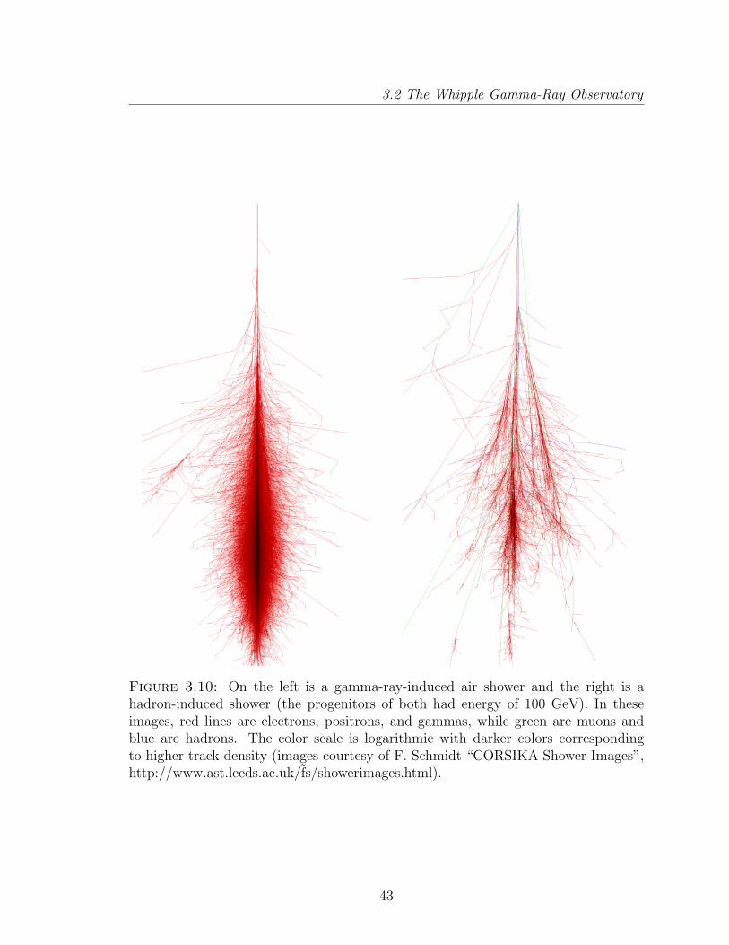
3.2 The Whipple Gamma-Ray Observatory
Figure 3.10: On the left is a gamma-ray-induced air shower and the right is ahadron-induced shower (the progenitors of both had energy of 100 GeV). In theseimages, red lines are electrons, positrons, and gammas, while green are muons andblue are hadrons. The color scale is logarithmic with darker colors correspondingto higher track density (images courtesy of F. Schmidt “CORSIKA Shower Images”,http://www.ast.leeds.ac.uk/fs/showerimages.html).
43
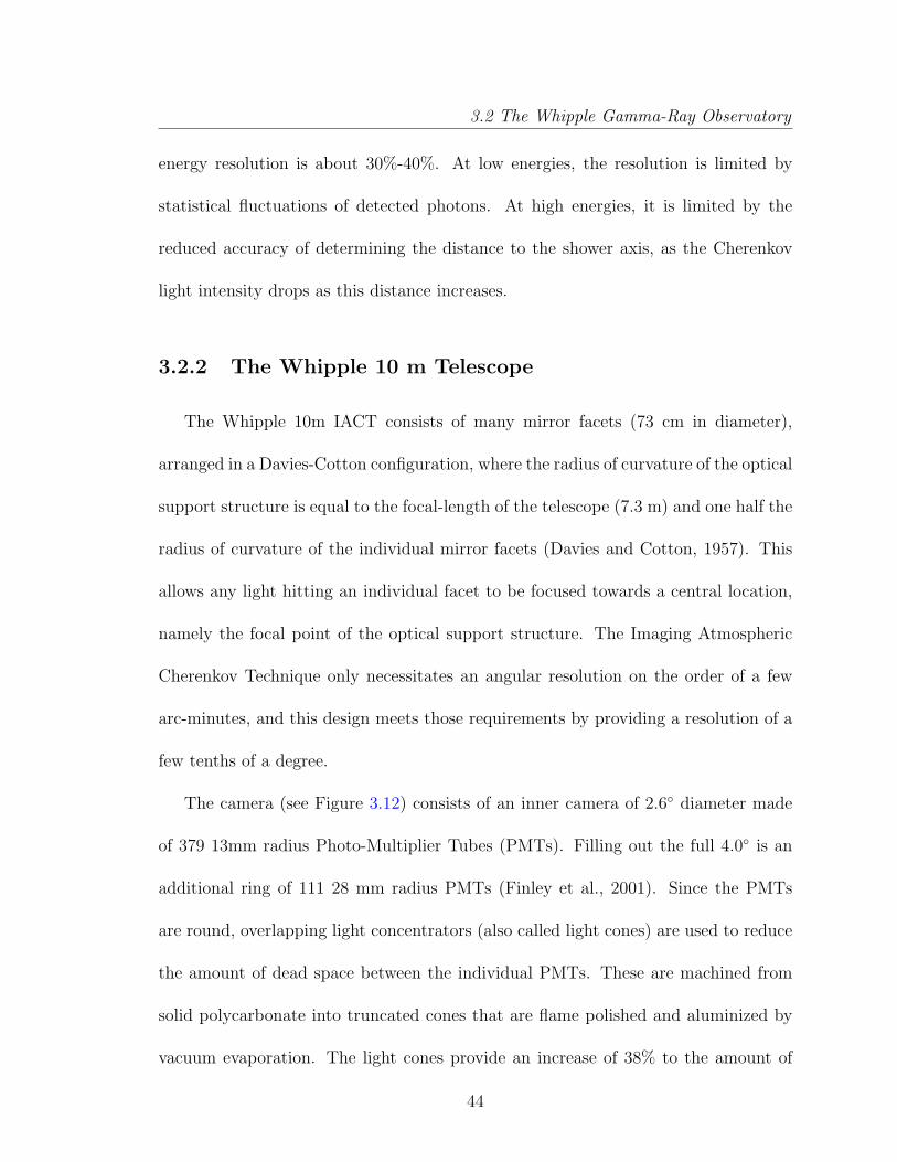
3.2 The Whipple Gamma-Ray Observatory
energy resolution is about 30%-40%. At low energies, the resolution is limited by
statistical fluctuations of detected photons. At high energies, it is limited by the
reduced accuracy of determining the distance to the shower axis, as the Cherenkov
light intensity drops as this distance increases.
3.2.2 The Whipple 10 m Telescope
The Whipple 10m IACT consists of many mirror facets (73 cm in diameter),
arranged in a Davies-Cotton configuration, where the radius of curvature of the optical
support structure is equal to the focal-length of the telescope (7.3 m) and one half the
radius of curvature of the individual mirror facets (Davies and Cotton, 1957). This
allows any light hitting an individual facet to be focused towards a central location,
namely the focal point of the optical support structure. The Imaging Atmospheric
Cherenkov Technique only necessitates an angular resolution on the order of a few
arc-minutes, and this design meets those requirements by providing a resolution of a
few tenths of a degree.
The camera (see Figure 3.12) consists of an inner camera of 2.6 diameter made
of 379 13mm radius Photo-Multiplier Tubes (PMTs). Filling out the full 4.0 is an
additional ring of 111 28 mm radius PMTs (Finley et al., 2001). Since the PMTs
are round, overlapping light concentrators (also called light cones) are used to reduce
the amount of dead space between the individual PMTs. These are machined from
solid polycarbonate into truncated cones that are flame polished and aluminized by
vacuum evaporation. The light cones provide an increase of 38% to the amount of
44
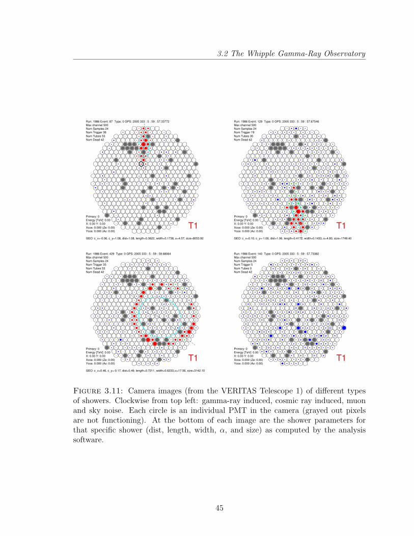
3.2 The Whipple Gamma-Ray Observatory
T1
Run: 1986 Event: 87 Type: 0 GPS: 2005 333 : 5 : 59 : 57.33772Max channel 500Num Samples 24Num Trigger 36Num Tubes 53Num Dead 42
=4.57, size=8053.92αGEO: c_x=-0.06, c_y=1.08, dist=1.08, length=0.3622, width=0.1738,
Primary: 0Energy [TeV]: 0.00X: 0.00 Y: 0.00Xcos: 0.000 (Ze: 0.00)Ycos: 0.000 (Az: 0.00)
T1
Run: 1986 Event: 129 Type: 0 GPS: 2005 333 : 5 : 59 : 57.67546Max channel 500Num Samples 24Num Trigger 19Num Tubes 35Num Dead 42
=4.80, size=1749.40αGEO: c_x=0.10, c_y=-1.06, dist=1.06, length=0.4172, width=0.1433,
Primary: 0Energy [TeV]: 0.00X: 0.00 Y: 0.00Xcos: 0.000 (Ze: 0.00)Ycos: 0.000 (Az: 0.00)
T1
Run: 1986 Event: 429 Type: 0 GPS: 2005 333 : 5 : 59 : 59.68064Max channel 500Num Samples 24Num Trigger 35Num Tubes 53Num Dead 42
=17.56, size=3142.10αGEO: c_x=0.46, c_y=-0.17, dist=0.49, length=0.7211, width=0.6233,
Primary: 0Energy [TeV]: 0.00X: 0.00 Y: 0.00Xcos: 0.000 (Ze: 0.00)Ycos: 0.000 (Az: 0.00)
T1
Run: 1986 Event: 140 Type: 0 GPS: 2005 333 : 5 : 59 : 57.73382Max channel 500Num Samples 24Num Trigger 5Num Tubes 0Num Dead 42
Primary: 0Energy [TeV]: 0.00X: 0.00 Y: 0.00Xcos: 0.000 (Ze: 0.00)Ycos: 0.000 (Az: 0.00)
Figure 3.11: Camera images (from the VERITAS Telescope 1) of different typesof showers. Clockwise from top left: gamma-ray induced, cosmic ray induced, muonand sky noise. Each circle is an individual PMT in the camera (grayed out pixelsare not functioning). At the bottom of each image are the shower parameters forthat specific shower (dist, length, width, α, and size) as computed by the analysissoftware.
45

3.2 The Whipple Gamma-Ray Observatory
Figure 3.12: The 10 m WhippleIACT’s 379 pixel camera, show-ing the focal plane and light-cones.The field of view of the center re-gion is ∼ 2.6 with the total fieldof view including the outer ring is4.0 (image from Kosack (2005)).
light collected by the camera (Finley et al., 2001). The angular size of the camera
pixels (∼ 0.2) matches the resolution needed to resolve a gamma-ray induced air
shower.
To reduce the total data rate while keeping the signal to noise level high, the
Whipple telescope operates in triggered mode only storing “shower-like” events for
later off-line analysis. The trigger system consists of two separate levels: the “pixel
trigger”, where a constant fraction discriminator (CFD) determines whether a single
pixel is triggered which is then digitized using a gated charge analog-to-digital con-
verter (QADC), and the “pattern trigger”, which requires that three (two and four
have also been used but not in this work) adjacent pixels fire.
46

Chapter 4
XMM-Newton X-ray Observations
of 3C 129
Some galaxy clusters are home to tailed radio galaxies and have drawn intensive
theoretical and observational astrophysical study for several decades. By observing
these enormous object with both Radio and X-ray instruments, one can produce high
resolution images of the extended synchrotron emission from the radio galaxy that
provides information on the energy density of the radio emitting plasma, magnetic
field and use the X-ray data to extract maps of the temperature, chemical composi-
tion, density and pressure of the ICM. The X-ray observations allow us to infer the
ICM properties and the jet propagates into a well-defined medium. Since the exact
composition of the ICM is known, one can study the pressure balance between the
radio-plasma and the ICM. Features such as cavities in the ICM where the plasma
from the radio source has displaced the ICM would show up as deficits in the X-ray
47
surface brightness. Boehringer et al. (1993) observed such cavities in the Perseus
cluster and Carilli et al. (1994) in Cygnus A. Recently there have been several more
observations in clusters Hydra A, Abell 2597, Abell 2052 and Abell 4059 (McNa-
mara et al., 2000, 2001; Blanton et al., 2001; Heinz et al., 2002; McNamara et al.,
2005). The galaxy cluster 3C 129, named for the prototypical head-tail radio galaxy
it contains, is one of the best clusters in which to observe such effects because it
is one of the largest (approximately 16’ long) radio jets known. Krawczynski et al.
(2003) previously observed this cluster with Chandra providing some very interesting
results (See Figure 4.1). Based on various radio data sets and the Chandra data they
studied the balance of the pressure in the radio tail and the ICM. Using the radio
observations of the radio galaxy, the pressure (and energy density) in the radio tail
can be constrained. Given the observed radio (synchrotron) luminosities in several
frequency bands Ls,i, the magnetic field that minimizes the energy density of the radio
synchrotron plasma (Pacholczyk, 1970) can be calculated:
Bmin =∑
i
(6 π)2/7 (1 + k)2/7 φ−2/7 V −2/7
(∑i
c12,i Ls,i
)2/7
(4.1)
where k describes the contribution to the non-thermal pressure from relativistic pro-
tons, V is the emitting volume, φ, is the volume filling factor, and c12,i are constants
that depend on the frequency band over which the luminosity Ls,i has been measured.
Thus, by looking at the radio emission from the jet, we can make estimates on the
energy density of the non-thermal radio plasma and from this, compute the minimum
pressure. Figure 4.2 shows the results of the pressure balance study. The tail seems
48
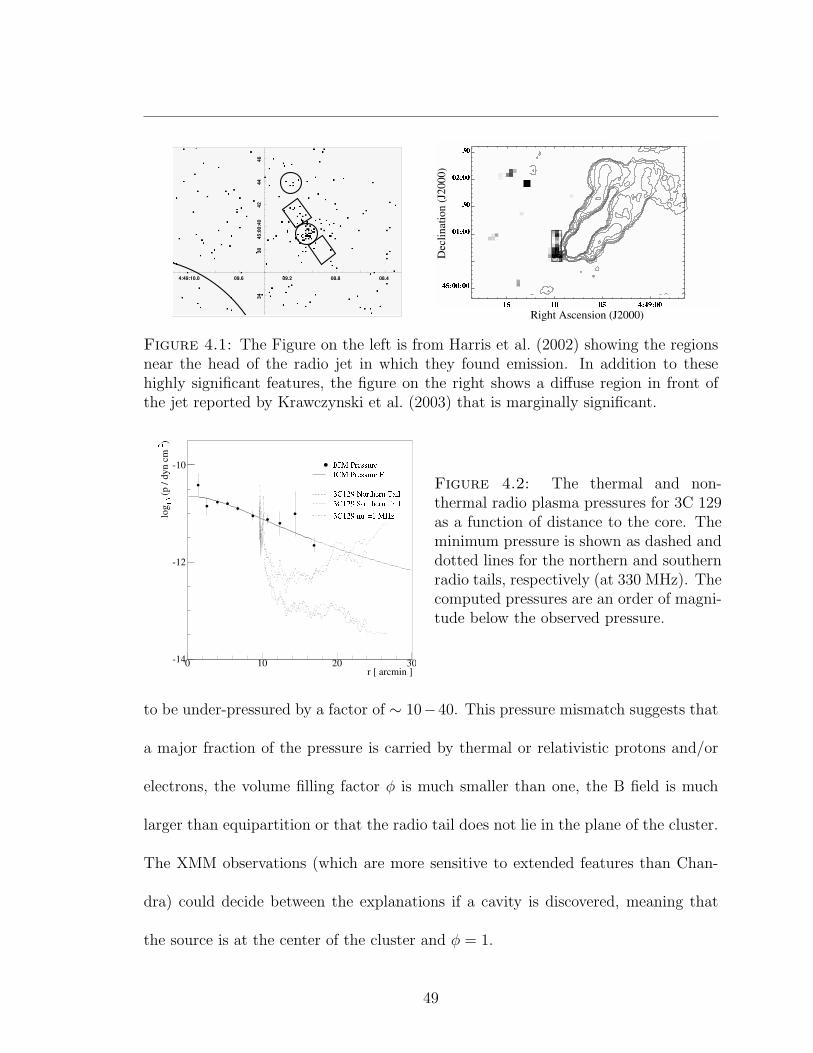
4:49:10.0 09.6 09.2 08.8 08.4
45:0
0:40
3834
4244
46
Right ascension
Decl
inat
ion
3C129
Figure 4.1: The Figure on the left is from Harris et al. (2002) showing the regionsnear the head of the radio jet in which they found emission. In addition to thesehighly significant features, the figure on the right shows a diffuse region in front ofthe jet reported by Krawczynski et al. (2003) that is marginally significant.
Figure 4.2: The thermal and non-thermal radio plasma pressures for 3C 129as a function of distance to the core. Theminimum pressure is shown as dashed anddotted lines for the northern and southernradio tails, respectively (at 330 MHz). Thecomputed pressures are an order of magni-tude below the observed pressure.
to be under-pressured by a factor of ∼ 10−40. This pressure mismatch suggests that
a major fraction of the pressure is carried by thermal or relativistic protons and/or
electrons, the volume filling factor φ is much smaller than one, the B field is much
larger than equipartition or that the radio tail does not lie in the plane of the cluster.
The XMM observations (which are more sensitive to extended features than Chan-
dra) could decide between the explanations if a cavity is discovered, meaning that
the source is at the center of the cluster and φ = 1.
49

4.1 Data Sets and Analysis
They also showed that there is a very localized core and jet emission as well as
possible diffuse emission directly in front of the jet (see Figure 4.1). For Chandra,
the core and jet emission are highly significant while the diffuse emission only showed
marginal significance. The diffuse emission has a greater excess than the core and
jet but its extended nature makes it more difficult to detect. Since XMM has worse
angular resolution than Chandra, we cannot hope to separate the emission from the
core from any diffuse emission in front of the jet because, even if the diffuse emission
exists, it will appear as part of the emission from the core (smeared into a single
point source). If there is some type of diffuse emission we would see it as a shift in
the center of gravity of the total emission and the addition of the two fluxes would
be greater than that seen from either of the separate sources seen with Chandra. In
the following chapter I first describe the search for cavities in the ICM of 3C 129
due to the radio plasma using a procedure of background subtraction developed by
Read and Ponman (2003). Following this, I look for an excess in emission before the
radio core and compare this with the Chandra results presented in Krawczynski et al.
(2003). Finally, I present the results of the optical monitor data. In the following
chapter, upper limits are presented at the two sigma level.
4.1 Data Sets and Analysis
The data consists of one pointing on February 18, 2003, with the MOS-1 and MOS-
2 chips along with the PN detector for a 50 ksec exposure proposed by H. Krawczynski
50
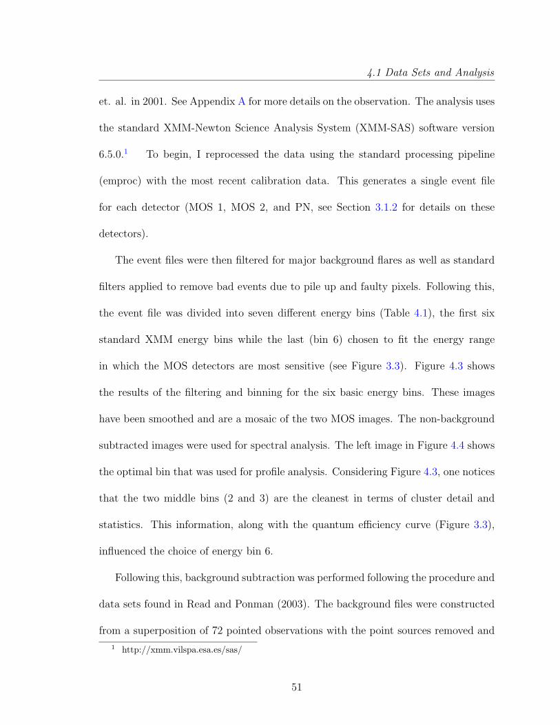
4.1 Data Sets and Analysis
et. al. in 2001. See Appendix A for more details on the observation. The analysis uses
the standard XMM-Newton Science Analysis System (XMM-SAS) software version
6.5.0.1 To begin, I reprocessed the data using the standard processing pipeline
(emproc) with the most recent calibration data. This generates a single event file
for each detector (MOS 1, MOS 2, and PN, see Section 3.1.2 for details on these
detectors).
The event files were then filtered for major background flares as well as standard
filters applied to remove bad events due to pile up and faulty pixels. Following this,
the event file was divided into seven different energy bins (Table 4.1), the first six
standard XMM energy bins while the last (bin 6) chosen to fit the energy range
in which the MOS detectors are most sensitive (see Figure 3.3). Figure 4.3 shows
the results of the filtering and binning for the six basic energy bins. These images
have been smoothed and are a mosaic of the two MOS images. The non-background
subtracted images were used for spectral analysis. The left image in Figure 4.4 shows
the optimal bin that was used for profile analysis. Considering Figure 4.3, one notices
that the two middle bins (2 and 3) are the cleanest in terms of cluster detail and
statistics. This information, along with the quantum efficiency curve (Figure 3.3),
influenced the choice of energy bin 6.
Following this, background subtraction was performed following the procedure and
data sets found in Read and Ponman (2003). The background files were constructed
from a superposition of 72 pointed observations with the point sources removed and
1 http://xmm.vilspa.esa.es/sas/
51
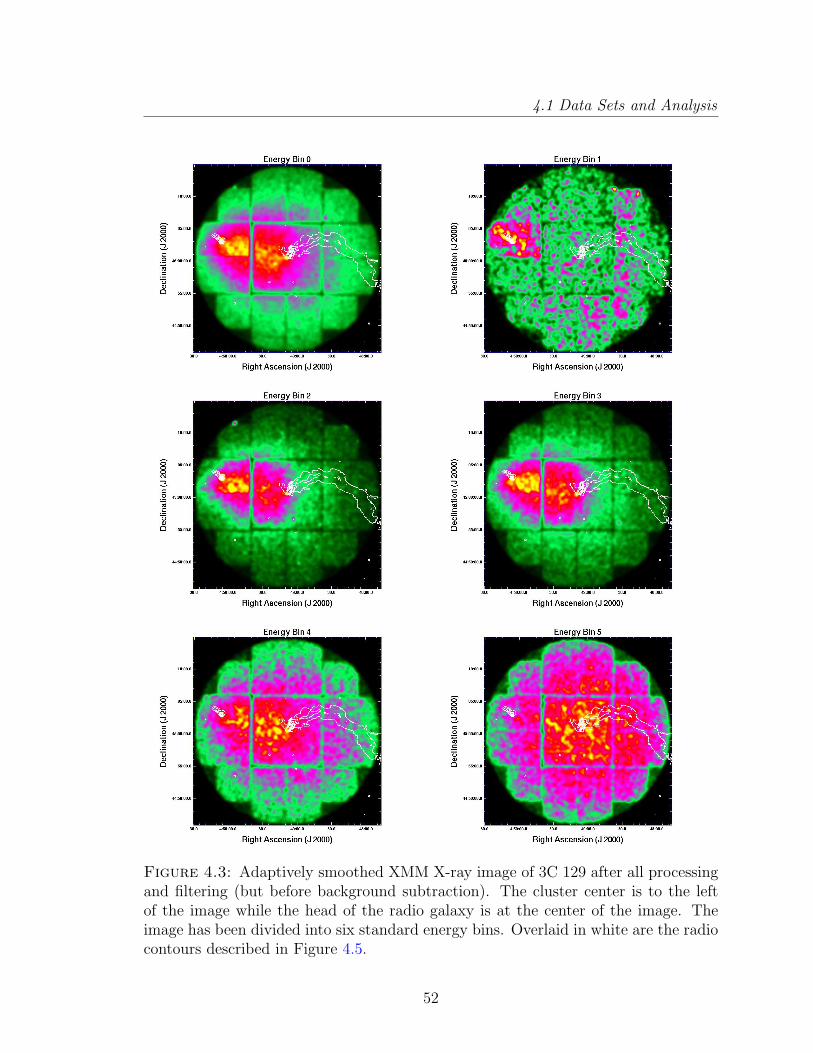
4.1 Data Sets and Analysis
Figure 4.3: Adaptively smoothed XMM X-ray image of 3C 129 after all processingand filtering (but before background subtraction). The cluster center is to the leftof the image while the head of the radio galaxy is at the center of the image. Theimage has been divided into six standard energy bins. Overlaid in white are the radiocontours described in Figure 4.5.
52

4.1 Data Sets and Analysis
Table 4.1: The energy bins used in this analysis. Bin 0 is the full range which issubsequently used for spectral analysis. Bins 0-5 are the standard XMM bins whilebin 6 is a bin chosen to best represent the capabilities of the MOS instrument.
Bin Number Energy Range (keV)0 0.2 - 121 0.2 - 0.52 0.5 - 23 2 - 4.54 4.5 - 7.55 7.5 - 126 0.7 - 4.5
are specific to an instrument and filter. These background files were “skycasted” to
match the sky coordinates of the 3C 129 observation. The event files were divided
into small energy bins of 100 eV before background subtraction and then rebuilt to
form the large energy bins afterwords. This was done to counteract an over-correcting
for exposure that can still be seen in the lowest energy bin (bin 1) and the two highest
bins (4 and 5), even with this correction. Thus, the final choice of energy bin used
in the extended analysis is bin 6, which can be seen as the energy range that is least
affected by this.
The subtraction process begins with an image created from the original (100 keV
wide) energy file. A background file and particle image is created from the blank-sky
background and a closed event file. The out of field of view events are used to scale
these images to correct any discrepancies in observation time. An exposure map and
exposure mask are also created (the exposure depends on the energy range desired and
this is where the small 100 keV energy bands are desirable: the exposure creation uses
53
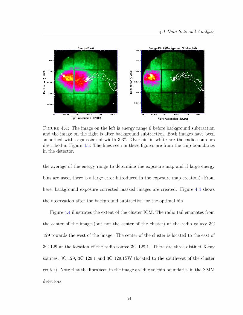
4.1 Data Sets and Analysis
Figure 4.4: The image on the left is energy range 6 before background subtractionand the image on the right is after background subtraction. Both images have beensmoothed with a gaussian of width 3.3′′. Overlaid in white are the radio contoursdescribed in Figure 4.5. The lines seen in these figures are from the chip boundariesin the detector.
the average of the energy range to determine the exposure map and if large energy
bins are used, there is a large error introduced in the exposure map creation). From
here, background exposure corrected masked images are created. Figure 4.4 shows
the observation after the background subtraction for the optimal bin.
Figure 4.4 illustrates the extent of the cluster ICM. The radio tail emanates from
the center of the image (but not the center of the cluster) at the radio galaxy 3C
129 towards the west of the image. The center of the cluster is located to the east of
3C 129 at the location of the radio source 3C 129.1. There are three distinct X-ray
sources, 3C 129, 3C 129.1 and 3C 129.1SW (located to the southwest of the cluster
center). Note that the lines seen in the image are due to chip boundaries in the XMM
detectors.
54

4.1 Data Sets and Analysis
Some of the features seen in the X-ray image have only modest statistical signif-
icance. To determine the statistical significance of any excess seen at a point in the
FoV, I use the number of counts in the ON region, NON , and compare this to the
number of counts found in a reasonable comparison OFF region, NOFF . I compute
the statistical significance based on Poisson probability distribution that accounts for
the statistical uncertainty in both the source and comparison region following the
method of Li and Ma (1983). The statistical significance of an excess is given in
standard deviations by:
S(NON, NOFF; ξ) =√−2 ln(λ) (4.2)
where
λ =
[ξ
ξ + 1
(NON + NOFF
NON
)]NON
× (4.3)[1
ξ + 1
(NON + NOFF
NOFF
)]NOFF
and ξ given by:
ξ =
∫∆ΩON
A(Ω) dΩ∫∆ΩOFF
A(Ω) dΩ(4.4)
where ∆ΩON and ∆ΩOFF are the solid angle areas of the source and background
regions, respectively, and A(Ω) is the the effective area of the detector. I use the
exposure map produced for the optimal energy range as A(Ω) and integrate over
this map with the CIAO2 tool dmstat. Although the method is based on Poisson
probability distributions, the expression for the statistical significance is only valid
for NON > 10 and NOFF > 10 (Alexandreas et al., 1993).
2 Chandra Interactive Analysis of Observations, http://cxc.harvard.edu/ciao/
55

4.2 Radio Tail Results
4.2 Radio Tail Results
The X-ray emission near 3C 129 is shown in Figures 4.5 and 4.6 along with the
radio contours. I searched for deficits in the ICM surface brightness along the radio
tails of the galaxy 3C 129. Figure 4.5 shows a zoomed in picture of the X-ray flux
from the cluster overlaid with a low resolution radio contours. This jet is over 17’
long with a width of between 13′, making it one of the largest of its kind. Figure
4.6 shows a high resolution radio contour image of the head of the jet detailing this
highly complicated region. The radio contours used here were all obtained using the
Very Large Array (VLA)3 and have been previously reported by Krawczynski et al.
(2003) in an analysis of this cluster with the Chandra observatory. The low resolution
contours are at a frequency of 1400 MHz while the high resolution images of the head
of the radio jet are at 5 GHz. Additionally, a high resolution 8 GHz map of 3C 129.1
has been used. Figure 4.7 is a profile of the X-ray flux along the line of the jet. The
first two bins cover the high resolution radio jets seen in Figure 4.6 and there is no
significant change in this region. There is a large decrease in flux showing some type
of change in the jet as it moves from the 5 GHz radio region and into the 1.4 GHz
region.
To search for deficits, I first optimized a search bin size for both the high resolution
and low resolution areas. For a rectangular jet of width 2′ and length ∼ 17′, I get an
optimal bin size of 3.33′, or slightly larger than the width of the jet. For a smaller
3 The National Radio Astronomy Observatory is a facility of the National Science Foundationoperated under cooperative agreement by Associated Universities, Inc.
56

4.2 Radio Tail Results
Figure 4.5: The colors (scaled linearly) show the background subtracted flat fieldedXMM 0.7 - 4.5 keV data (MOS 1 and MOS 2) smoothed with a Gaussian of width5′′. The 1400 MHz radio contours detail the radio tail spanning over 17′ in lengthand 3′ at its largest width. The contours are drawn at 0.0025, 0.035, 0.08, 0.12, 0.15,and 0.20 beam−1 with a beam-width of 8′′ FWHM.
Figure 4.6: The colors (scaledlinearly) show the backgroundsubtracted flat fielded XMM 0.7- 4.5 keV data (MOS1 and MOS2) smoothed with a gaussian ofwidth 5”. The radio contours arefrom 5 GHz VLA data with a 1.8”FWHM beam-width and a loga-rithmically spaced from 1 to 32mJy beam−1.
57
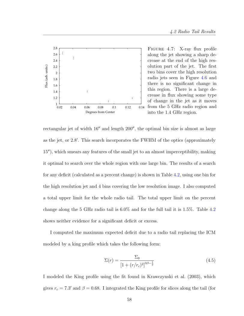
4.2 Radio Tail Results
1
1.2
1.4
1.6
1.8
2
2.2
2.4
2.6
2.8
0.02 0.04 0.06 0.08 0.1 0.12 0.14
Flux
(arb
. uni
ts.)
Degrees from Center
Figure 4.7: X-ray flux profilealong the jet showing a sharp de-crease at the end of the high res-olution part of the jet. The firsttwo bins cover the high resolutionradio jets seen in Figure 4.6 andthere is no significant change inthis region. There is a large de-crease in flux showing some typeof change in the jet as it movesfrom the 5 GHz radio region andinto the 1.4 GHz region.
rectangular jet of width 16′′ and length 200′′, the optimal bin size is almost as large
as the jet, or 2.8′. This search incorporates the FWHM of the optics (approximately
15′′), which smears any features of the small jet to an almost imperceptibility, making
it optimal to search over the whole region with one large bin. The results of a search
for any deficit (calculated as a percent change) is shown in Table 4.2, using one bin for
the high resolution jet and 4 bins covering the low resolution image. I also computed
a total upper limit for the whole radio tail. The total upper limit on the percent
change along the 5 GHz radio tail is 6.0% and for the full tail it is 1.5%. Table 4.2
shows neither evidence for a significant deficit or excess.
I computed the maximum expected deficit due to a radio tail replacing the ICM
modeled by a king profile which takes the following form:
Σ(r) =Σ0
[1 + (r/rc)2]3β− 12
(4.5)
I modeled the King profile using the fit found in Krawczynski et al. (2003), which
gives rc = 7.3′ and β = 0.68. I integrated the King profile for slices along the tail (for
58

4.3 Spectra
Table 4.2: Upper limits on the fractional X-ray flux deficits for each bin. The jetshown by the high resolution radio contours was covered by a single bin while the lowresolution jet with 4. The total of the 4 bins is also reported. Note that a negativechange means that there is a deficit in the radio jet compared to the backgroundregion.
Jet Bin % Change Statistical Fractional DeficitError Upper Limits
5 GHz VLA 0 1.6 3.1 6.01.4 GHz VLA 0 4.8 1.8 1.91.4 GHz VLA 1 3.5 2.3 3.41.4 GHz VLA 2 1.6 2.1 3.81.4 GHz VLA 3 -3.8 2.1 8.11.4 GHz VLA total 1.5 1.0 1.5
distances of 10′, 12′, 14′, and 16′ from the cluster core). Table 4.3 shows the results of
this calculation. The average change is 10%, which represents the maximum expected
change and our actual upper limits are all below this. This shows that the deficit is
smaller than expected. We can tentatively conclude that the radio tail does not only
consist of non-thermal plasma, but that it is mixed with the thermal ICM along the
tail. If the tail, however, does not lie in the central plane of the cluster (which is an
assumption of the above calculation), then the expected deficit may be small even if
it fully consists of non-thermal plasma.
4.3 Spectra
There are three regions of interest for spectral analysis, the two hot spots at the
core of the cluster and the head of the radio jet. In the following section I will report
on the spectral fitting of these three regions. I used the XMM full images from 0.2
59
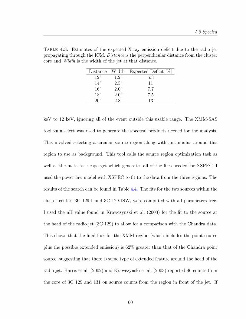
4.3 Spectra
Table 4.3: Estimates of the expected X-ray emission deficit due to the radio jetpropagating through the ICM. Distance is the perpendicular distance from the clustercore and Width is the width of the jet at that distance.
Distance Width Expected Deficit [%]12’ 1.2’ 5.314’ 2.5’ 1116’ 2.0’ 7.718’ 2.0’ 7.520’ 2.8’ 13
keV to 12 keV, ignoring all of the event outside this usable range. The XMM-SAS
tool xmmselect was used to generate the spectral products needed for the analysis.
This involved selecting a circular source region along with an annulus around this
region to use as background. This tool calls the source region optimization task as
well as the meta task especget which generates all of the files needed for XSPEC. I
used the power law model with XSPEC to fit to the data from the three regions. The
results of the search can be found in Table 4.4. The fits for the two sources within the
cluster center, 3C 129.1 and 3C 129.1SW, were computed with all parameters free.
I used the nH value found in Krawczynski et al. (2003) for the fit to the source at
the head of the radio jet (3C 129) to allow for a comparison with the Chandra data.
This shows that the final flux for the XMM region (which includes the point source
plus the possible extended emission) is 62% greater than that of the Chandra point
source, suggesting that there is some type of extended feature around the head of the
radio jet. Harris et al. (2002) and Krawczynski et al. (2003) reported 46 counts from
the core of 3C 129 and 131 on source counts from the region in front of the jet. If
60
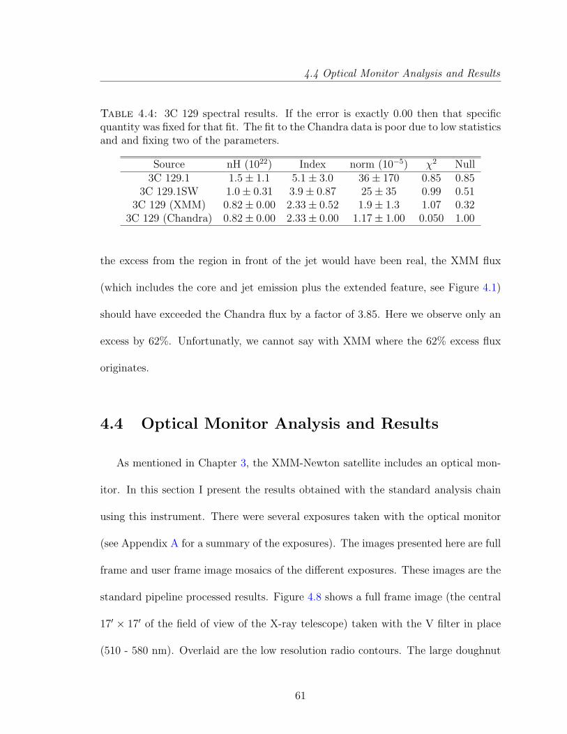
4.4 Optical Monitor Analysis and Results
Table 4.4: 3C 129 spectral results. If the error is exactly 0.00 then that specificquantity was fixed for that fit. The fit to the Chandra data is poor due to low statisticsand and fixing two of the parameters.
Source nH (1022) Index norm (10−5) χ2 Null3C 129.1 1.5± 1.1 5.1± 3.0 36± 170 0.85 0.85
3C 129.1SW 1.0± 0.31 3.9± 0.87 25± 35 0.99 0.513C 129 (XMM) 0.82± 0.00 2.33± 0.52 1.9± 1.3 1.07 0.32
3C 129 (Chandra) 0.82± 0.00 2.33± 0.00 1.17± 1.00 0.050 1.00
the excess from the region in front of the jet would have been real, the XMM flux
(which includes the core and jet emission plus the extended feature, see Figure 4.1)
should have exceeded the Chandra flux by a factor of 3.85. Here we observe only an
excess by 62%. Unfortunatly, we cannot say with XMM where the 62% excess flux
originates.
4.4 Optical Monitor Analysis and Results
As mentioned in Chapter 3, the XMM-Newton satellite includes an optical mon-
itor. In this section I present the results obtained with the standard analysis chain
using this instrument. There were several exposures taken with the optical monitor
(see Appendix A for a summary of the exposures). The images presented here are full
frame and user frame image mosaics of the different exposures. These images are the
standard pipeline processed results. Figure 4.8 shows a full frame image (the central
17′ × 17′ of the field of view of the X-ray telescope) taken with the V filter in place
(510 - 580 nm). Overlaid are the low resolution radio contours. The large doughnut
61
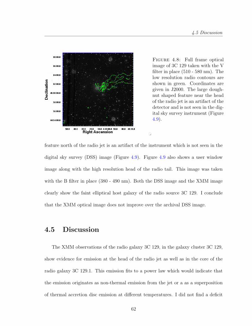
4.5 Discussion
Figure 4.8: Full frame opticalimage of 3C 129 taken with the Vfilter in place (510 - 580 nm). Thelow resolution radio contours areshown in green. Coordinates aregiven in J2000. The large dough-nut shaped feature near the headof the radio jet is an artifact of thedetector and is not seen in the dig-ital sky survey instrument (Figure4.9).
feature north of the radio jet is an artifact of the instrument which is not seen in the
digital sky survey (DSS) image (Figure 4.9). Figure 4.9 also shows a user window
image along with the high resolution head of the radio tail. This image was taken
with the B filter in place (380 - 490 nm). Both the DSS image and the XMM image
clearly show the faint elliptical host galaxy of the radio source 3C 129. I conclude
that the XMM optical image does not improve over the archival DSS image.
4.5 Discussion
The XMM observations of the radio galaxy 3C 129, in the galaxy cluster 3C 129,
show evidence for emission at the head of the radio jet as well as in the core of the
radio galaxy 3C 129.1. This emission fits to a power law which would indicate that
the emission originates as non-thermal emission from the jet or a as a superposition
of thermal accretion disc emission at different temperatures. I did not find a deficit
62

4.5 Discussion
Figure 4.9: On the left is a zoomed in optical image of 3C 129 taken with the Bfilter in place (390 - 490 nm). On the right is an archival digital sky survey image ofthe same region clearly showing the faint elliptical host galaxy as well as confirmingthe large doughnut region in the XMM images is an artifact of the instrument. Thehigh resolution VLA contours are shown in green. Coordinates are given in J2000.
in the ICM emissivity associated with the the radio tail which would indicate that
the tail replaced ICM. Here I computed upper limits on the fractional deficit and find
that it is 6% for the portion nearest the head and 1.5% for the full radio tail although
segments of the tail have upper limits as high as 8%. Further analysis, based on
spectral fitting of the core, shows that there is 62% more emission in the XMM data
than in the Chandra observation, suggesting that there is some extended emission in
addition to the core and jet emission seen by Chandra. The optical monitor shows
the existence of a faint elliptical galaxy hosting the head of the radio jet.
63

Chapter 5
TeV Observations of the Perseus
and A2029 Clusters with the
Whipple 10 m Telescope
5.1 Data and Analysis
The following chapter describes a search for TeV emission from the Perseus and
Abell 2029 galaxy clusters using the Whipple 10 m Cherenkov telescope (see Chapter
3). The chapter is organized as follows: I describe the observations, data cleaning
procedures, and the data analysis methods in Section 5.1. The main results of this
study are a search for point source emission from localized sources in the clusters and
a search for diffuse emission from the ICM. I present these results in Section 5.2 and
discuss them in Section 5.3. Reported uncertainties are one standard deviation and
64
5.1 Data and Analysis
upper limits are given at the 90% confidence level, unless otherwise stated.
There are limitations to observing extended sources with a single Cherenkov tele-
scope like the Whipple 10 m. First, the sensitivity of the telescope falls for angular
distances greater than 0.8 degrees from the center of the field of view. Churazov
et al. (2003) shows a high temperature region in the Perseus cluster, at about 0.25
degrees from the cluster center, that might be associated with shocks and possibly
emit VHE emission. Even though we theoretically could study such shocks, we do
not perform a specialized search for merger related emission. In the case of the more
distant cluster A2029, our search region of 0.8 degree radius covers a physical region
of 4.2 Mpc radius. Thus, our search includes all the cluster emission, independent of
where in the cluster it originates.
5.1.1 Instrumentation and Data Sets
We observed the Perseus cluster between August 16, 2004, and February 5, 2005
(UT). Data were taken as pairs of 28 minute runs. An ON run pointed at the source
was followed by an OFF run at the same azimuth and elevation but offset 7.50 (30
minutes) in right ascension for background subtraction. Even though care was taken
to observe during the clearest of nights, some runs had low rates and were removed.
There were also situations in which the sky conditions differed between the ON/OFF
pairs, and these were also removed, resulting in a total of 29 ON/OFF pairs for
analysis. Performing the same selection on the Abell 2029, observations (observed
between March 7, 2003, and May 5, 2003 (UT)) resulted in 14 ON/OFF pairs. In
65

5.1 Data and Analysis
13000
14000
15000
16000
17000
18000
19000
20000
5 10 15 20 25 30 35
Cos
mic
Ray
Cou
nts
Zenith Angle (Degrees)
CrabPerseus
Perseus FitFigure 5.1: Cosmic Ray countson a run by run basis versus zenithangle. Shown are data from theCrab Nebula (open circles) andthe Perseus Cluster (closed cir-cles). We fitted each group of data(see the Perseus Fit line for an ex-ample) to show the dependence ofthe rate on the zenith angle andrejected any runs that deviated bymore than 10%.
Table 5.1: Description of the various data sets used in this analysis. The Crabsets titled “Crab-0.5” and “Crab-0.8” are observations performed with the telescopeoffset from the location of the Crab nebula by 0.5 and 0.8, respectively.
Source Season Number ON OFF(MJD) (Pairs) (min) (min)
Perseus 2004-2005 29 810.4 810.4Abell 2029 2003-2004 13 363.3 363.3
Crab 2003-2004 29 810.4 810.4Crab 2004-2005 24 670.7 670.4
Crab-0.5 2003-2005 6 167.7 167.6Crab-0.8 2003-2005 8 223.6 223.6
addition to the cluster observations, a number of observations of the Crab Nebula
(a “Standard Candle” in TeV gamma-ray astronomy) were taken to determine the
detection efficiency and angular resolution for various points on the camera. The
cosmic ray rates of each run versus the zenith angle are shown in Figure 5.1 to
illustrate how the pair selection is done (by rejecting those runs that deviate more
than 10% from the expected rate). Table 5.1 details the duration and observing
season of the various data sets and Appendix B thoroughly lists the details for each
run.
66
5.1 Data and Analysis
5.1.2 Standard Analysis
After determining which runs to include, the data were analyzed using the stan-
dard 2nd-moment-parametrization technique (Hillas, 1985). We identify gamma-ray
events and suppress background cosmic ray events by applying gamma-ray selection
criteria (EZCuts2004, see (Kosack, 2005)), designed to be independent of zenith angle
and energy and well suited for the analysis of extended sources. The 2D arrival di-
rection of each gamma-ray event was calculated from the orientation and elongation
of the Cherenkov light distribution in the camera (Buckley et al., 1998). We estimate
that the mean energy threshold for the Whipple 10 m to be approximately 400 GeV
(Finley et al., 2001). More detailed descriptions of Whipple observing modes and
analysis procedures have been given by (Weekes, 1996), (Punch and Fegan, 1991),
and (Reynolds et al., 1993).
5.1.3 Cluster Specific Analysis
In this section we describe the specific analysis techniques applied to the clusters,
including the method used to search for point sources within each cluster. Based on
the expected lateral emission profiles, we then discuss the examination of the cluster
for diffuse emission.
The initial analysis of the clusters involves a search for point sources before the
analysis of any extended emission. It is a result in itself if point sources exist but
then they must be excluded from the extended emission analysis. The atmospheric
67

5.1 Data and Analysis
Cherenkov technique was originally designed for the observation of point sources
at the center of the field-of-view. Thus, the resolution and detection efficiency is
not optimal off center but to search for point sources at any point in the field of
view, we need to determine better these factors at all camera locations. Using data
from the Crab Nebula that were taken during the same time frame as the cluster
observations, we used an empirical method to determine the telescope properties.
The background-subtracted Crab data were binned by the square of the distance of
the reconstructed shower direction from the location of the Crab Nebula (so as to
eliminate any solid angle dependence) and fitted with an exponential. These fits gave
us a direct measurement of the angular resolution of the camera for a point source at
different locations within the field-of-view. From these same data, we determined an
optimal angular cut based on the integral number of excess and background counts as
a function of angular distance from the source location. By calculating the gamma-
ray rate at the different offsets, we also determined how the efficiency of the camera
falls off towards the edges.
This empirical method was compared to Monte Carlo simulations of centered
and offset data. The Monte Carlo code1 simulates atmospheric Cherenkov showers
and calculates the response of the Whipple detector. The simulated data have the
same format as the experimental data and were analyzed using the same methods as
those applied to the real data. We produced a simulated shower set with a differential
spectral index of -2.5 and fed this through the detector simulations for different source
1http://www.physics.utah.edu/gammaray/GrISU/
68
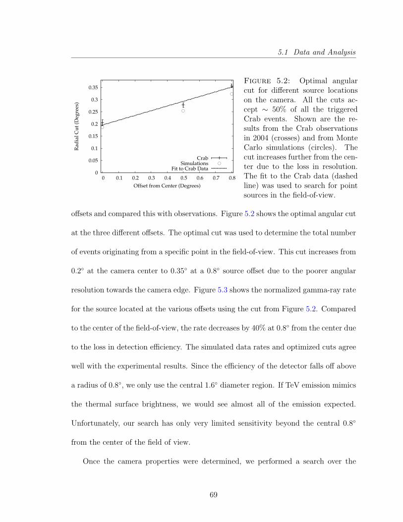
5.1 Data and Analysis
0
0.05
0.1
0.15
0.2
0.25
0.3
0.35
0 0.1 0.2 0.3 0.4 0.5 0.6 0.7 0.8
Rad
ial
Cu
t (D
egre
es)
Offset from Center (Degrees)
CrabSimulations
Fit to Crab Data
Figure 5.2: Optimal angularcut for different source locationson the camera. All the cuts ac-cept ∼ 50% of all the triggeredCrab events. Shown are the re-sults from the Crab observationsin 2004 (crosses) and from MonteCarlo simulations (circles). Thecut increases further from the cen-ter due to the loss in resolution.The fit to the Crab data (dashedline) was used to search for pointsources in the field-of-view.
offsets and compared this with observations. Figure 5.2 shows the optimal angular cut
at the three different offsets. The optimal cut was used to determine the total number
of events originating from a specific point in the field-of-view. This cut increases from
0.2 at the camera center to 0.35 at a 0.8 source offset due to the poorer angular
resolution towards the camera edge. Figure 5.3 shows the normalized gamma-ray rate
for the source located at the various offsets using the cut from Figure 5.2. Compared
to the center of the field-of-view, the rate decreases by 40% at 0.8 from the center due
to the loss in detection efficiency. The simulated data rates and optimized cuts agree
well with the experimental results. Since the efficiency of the detector falls off above
a radius of 0.8, we only use the central 1.6 diameter region. If TeV emission mimics
the thermal surface brightness, we would see almost all of the emission expected.
Unfortunately, our search has only very limited sensitivity beyond the central 0.8
from the center of the field of view.
Once the camera properties were determined, we performed a search over the
69
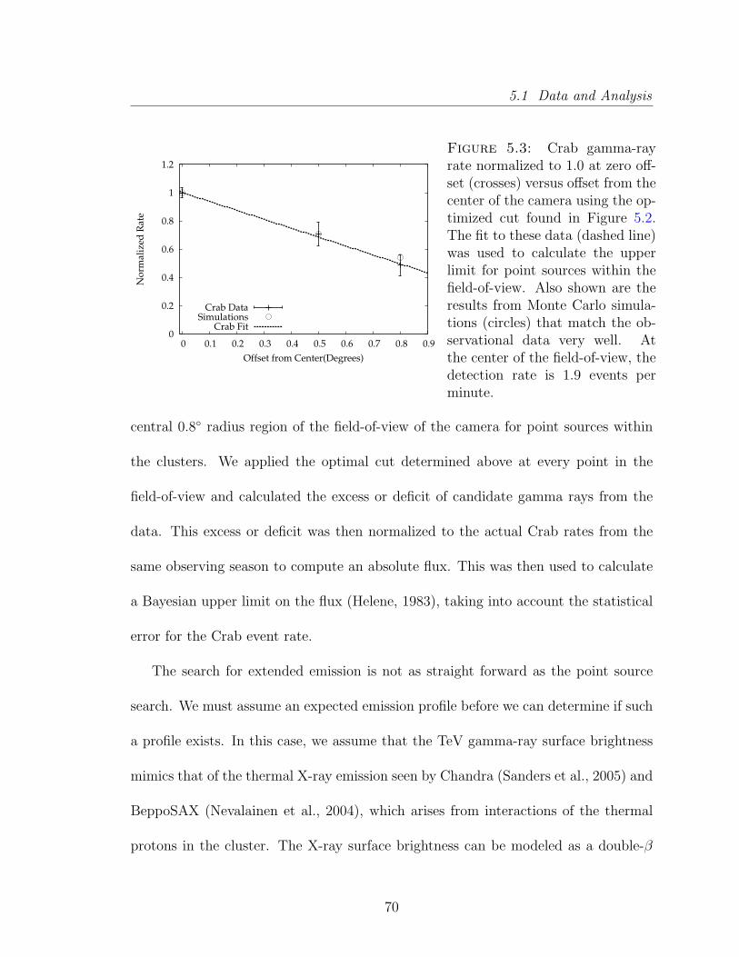
5.1 Data and Analysis
0
0.2
0.4
0.6
0.8
1
1.2
0 0.1 0.2 0.3 0.4 0.5 0.6 0.7 0.8 0.9
No
rmal
ized
Rat
e
Offset from Center(Degrees)
Crab DataSimulations
Crab Fit
Figure 5.3: Crab gamma-rayrate normalized to 1.0 at zero off-set (crosses) versus offset from thecenter of the camera using the op-timized cut found in Figure 5.2.The fit to these data (dashed line)was used to calculate the upperlimit for point sources within thefield-of-view. Also shown are theresults from Monte Carlo simula-tions (circles) that match the ob-servational data very well. Atthe center of the field-of-view, thedetection rate is 1.9 events perminute.
central 0.8 radius region of the field-of-view of the camera for point sources within
the clusters. We applied the optimal cut determined above at every point in the
field-of-view and calculated the excess or deficit of candidate gamma rays from the
data. This excess or deficit was then normalized to the actual Crab rates from the
same observing season to compute an absolute flux. This was then used to calculate
a Bayesian upper limit on the flux (Helene, 1983), taking into account the statistical
error for the Crab event rate.
The search for extended emission is not as straight forward as the point source
search. We must assume an expected emission profile before we can determine if such
a profile exists. In this case, we assume that the TeV gamma-ray surface brightness
mimics that of the thermal X-ray emission seen by Chandra (Sanders et al., 2005) and
BeppoSAX (Nevalainen et al., 2004), which arises from interactions of the thermal
protons in the cluster. The X-ray surface brightness can be modeled as a double-β
70
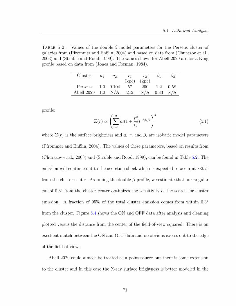
5.1 Data and Analysis
Table 5.2: Values of the double-β model parameters for the Perseus cluster ofgalaxies from (Pfrommer and Enßlin, 2004) and based on data from (Churazov et al.,2003) and (Struble and Rood, 1999). The values shown for Abell 2029 are for a Kingprofile based on data from (Jones and Forman, 1984).
Cluster a1 a2 r1 r2 β1 β2
(kpc) (kpc)Perseus 1.0 0.104 57 200 1.2 0.58
Abell 2029 1.0 N/A 212 N/A 0.83 N/A
profile:
Σ(r) ∝
(2∑
i=1
ai(1 +r2
r2i
)−3βi/2
)2
(5.1)
where Σ(r) is the surface brightness and ai, ri and βi are isobaric model parameters
(Pfrommer and Enßlin, 2004). The values of these parameters, based on results from
(Churazov et al., 2003) and (Struble and Rood, 1999), can be found in Table 5.2. The
emission will continue out to the accretion shock which is expected to occur at ∼2.2
from the cluster center. Assuming the double-β profile, we estimate that our angular
cut of 0.3 from the cluster center optimizes the sensitivity of the search for cluster
emission. A fraction of 95% of the total cluster emission comes from within 0.3
from the cluster. Figure 5.4 shows the ON and OFF data after analysis and cleaning
plotted versus the distance from the center of the field-of-view squared. There is an
excellent match between the ON and OFF data and no obvious excess out to the edge
of the field-of-view.
Abell 2029 could almost be treated as a point source but there is some extension
to the cluster and in this case the X-ray surface brightness is better modeled in the
71

5.1 Data and Analysis
)2 (Degrees2Distance0 0.5 1 1.5 2 2.5 3 3.5 4
Cou
nts
0
500
1000
1500
2000
2500
3000
3500
4000
Figure 5.4: Number of Whipple10 m Perseus observation eventsversus the distance of the esti-mated arrival direction from thecenter of the field-of-view squared.The dashed line shows the OFFcounts and the solid line the ONcounts. There is a good match be-tween the ON and the OFF dataout to the edge of the camera, andno excess from the cluster is de-tected.
case of Abell 2029 by a single-β King profile (King, 1972) given by
Σ(r) ∝ ai(1 +r2
r21
)−3β1+1/2. (5.2)
The model parameters are found in Table 5.2 and are from (Jones and Forman, 1984),
based upon observations made with the Einstein observatory. We chose the Einstein
observations over more recent observations by Chandra due to the larger field-of-view
of Einstein. For this cluster, the X-ray emission continues out to ∼1.0 from the
center of the cluster, and 96% of the emission comes from the central 0.3.
We then determined quantitative upper limits by normalizing these profiles over
the field-of-view of the camera. This was then convolved with the point spread func-
tion of the Whipple telescope (which widens the profile even more) and multiplied
by the offset-dependent Crab detection rate. The method generates a map of the
expected detection rate, assuming that the entire cluster produces the same TeV flux
as the Crab Nebula (using this we can determine a flux normalized to the Crab for the
full cluster). Figure 5.5 shows the expected emission based on the double-β profile for
72
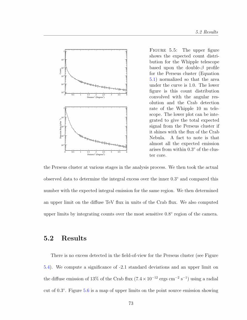
5.2 Results
) 2 (Degrees2Distance0 0.5 1 1.5 2 2.5 3 3.5 4
Cou
nts
-510
-410
-310
-210
-110
1
)2 (Degrees2Distance0 0.5 1 1.5 2 2.5 3 3.5 4
)-1
bin
γD
etec
tion
Rat
e (
-410
-310
-210
-110
1
Figure 5.5: The upper figureshows the expected count distri-bution for the Whipple telescopebased upon the double-β profilefor the Perseus cluster (Equation5.1) normalized so that the areaunder the curve is 1.0. The lowerfigure is this count distributionconvolved with the angular res-olution and the Crab detectionrate of the Whipple 10 m tele-scope. The lower plot can be inte-grated to give the total expectedsignal from the Perseus cluster ifit shines with the flux of the CrabNebula. A fact to note is thatalmost all the expected emissionarises from within 0.3 of the clus-ter core.
the Perseus cluster at various stages in the analysis process. We then took the actual
observed data to determine the integral excess over the inner 0.3 and compared this
number with the expected integral emission for the same region. We then determined
an upper limit on the diffuse TeV flux in units of the Crab flux. We also computed
upper limits by integrating counts over the most sensitive 0.8 region of the camera.
5.2 Results
There is no excess detected in the field-of-view for the Perseus cluster (see Figure
5.4). We compute a significance of -2.1 standard deviations and an upper limit on
the diffuse emission of 13% of the Crab flux (7.4×10⁻¹² ergs cm−2 s−1) using a radial
cut of 0.3. Figure 5.6 is a map of upper limits on the point source emission showing
73
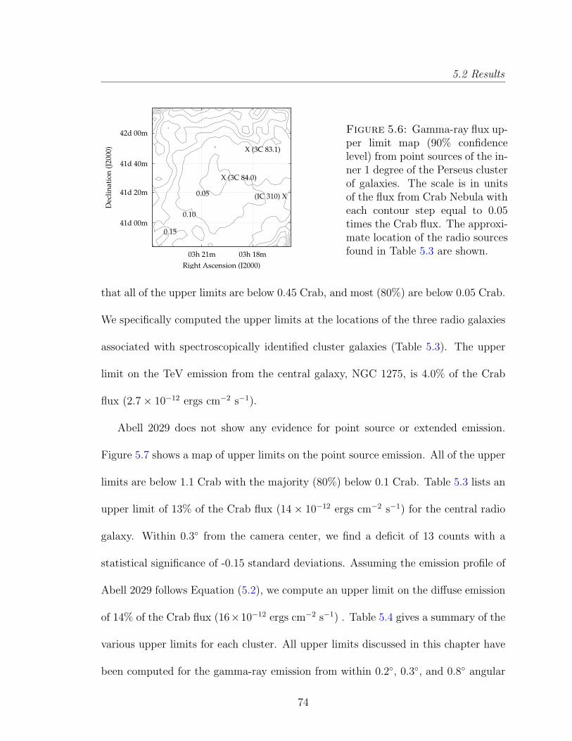
5.2 Results
42d 00m
41d 40m
41d 20m
41d 00m
03h 18m03h 21m
Dec
lin
atio
n (
J200
0)
Right Ascension (J2000)
X (3C 84.0)
(IC 310) X
X (3C 83.1)
0.05
0.10
0.15
Figure 5.6: Gamma-ray flux up-per limit map (90% confidencelevel) from point sources of the in-ner 1 degree of the Perseus clusterof galaxies. The scale is in unitsof the flux from Crab Nebula witheach contour step equal to 0.05times the Crab flux. The approxi-mate location of the radio sourcesfound in Table 5.3 are shown.
that all of the upper limits are below 0.45 Crab, and most (80%) are below 0.05 Crab.
We specifically computed the upper limits at the locations of the three radio galaxies
associated with spectroscopically identified cluster galaxies (Table 5.3). The upper
limit on the TeV emission from the central galaxy, NGC 1275, is 4.0% of the Crab
flux (2.7× 10⁻¹² ergs cm−2 s−1).
Abell 2029 does not show any evidence for point source or extended emission.
Figure 5.7 shows a map of upper limits on the point source emission. All of the upper
limits are below 1.1 Crab with the majority (80%) below 0.1 Crab. Table 5.3 lists an
upper limit of 13% of the Crab flux (14× 10−12 ergs cm−2 s−1) for the central radio
galaxy. Within 0.3 from the camera center, we find a deficit of 13 counts with a
statistical significance of -0.15 standard deviations. Assuming the emission profile of
Abell 2029 follows Equation (5.2), we compute an upper limit on the diffuse emission
of 14% of the Crab flux (16×10−12 ergs cm−2 s−1) . Table 5.4 gives a summary of the
various upper limits for each cluster. All upper limits discussed in this chapter have
been computed for the gamma-ray emission from within 0.2, 0.3, and 0.8 angular
74

5.3 Interpretation and Discussion
Perseus Abell 2029Source 3C 84.0 3C 83.1 IC 310 IC 11
(NGC 1275) (NGC 1265)RA 03 19 48 03 18 16 03 16 43 15 10 56
(J2000)DEC +41 30 42 +41 51 27 +41 19 29 +05 44 42
(J2000)20 cm Flux 2829.2 1305.5 168.1 527.8
(mJy)400 GeV Upper Limit 0.047 0.086 0.13 0.13
(Crab)400 GeV Upper Limit 0.29 0.53 0.80 1.1(10−11ergs cm−2 s−1)
Table 5.3: Gamma-ray flux 90% upper limits on spectroscopically resolved radiogalaxies associated with members of the Perseus and Abell 2029 clusters of galaxies.The 20 cm flux data are from The NRAO VLA Sky Survey (Condon et al., 1998).
distance from the cluster core. Flux upper limits have been scaled based upon the
assumed spectral shape after absorption.
5.3 Interpretation and Discussion
The final result of our search for TeV emission from the Perseus and Abell 2029
clusters of galaxies is shown in Figure 5.8 compared with previous upper limits from
EGRET (Reimer et al., 2003), and the results of model calculations. The lines show
models of the CRp induced gamma-ray emission normalized to the EGRET upper
limits, assuming a CRp spectrum with differential spectral index of -2.1 (Pfrommer
and Enßlin, 2004). This index is a reasonable choice of the source spectrum because
galaxy clusters are not “leaky” and retain all CRp, unlike our Galaxy where leakage
75
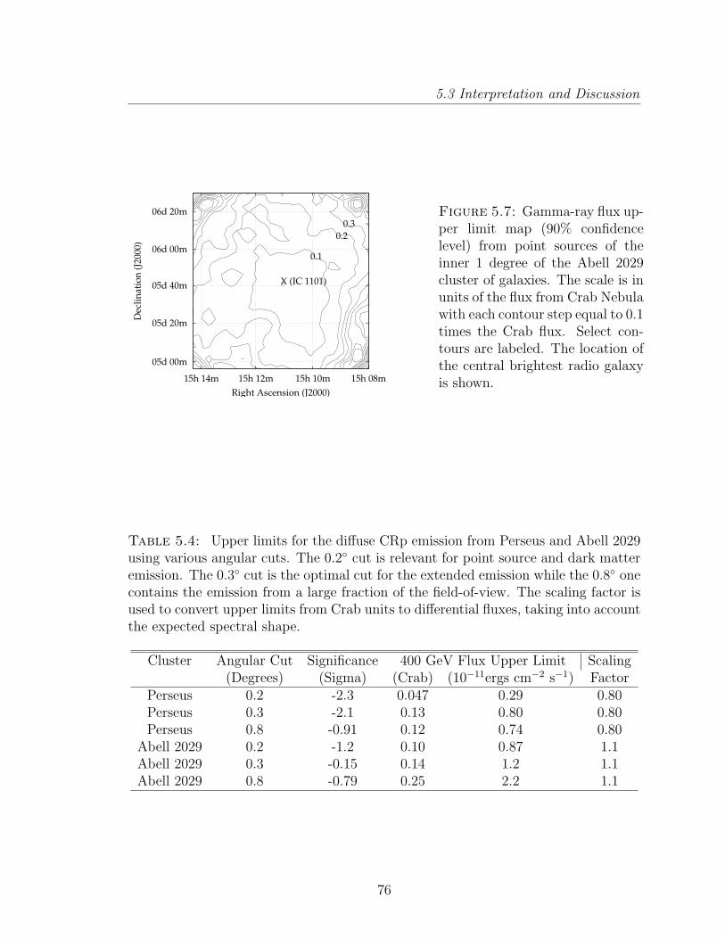
5.3 Interpretation and Discussion
06d 20m
06d 00m
05d 40m
05d 20m
05d 00m
15h 08m15h 10m15h 12m15h 14m
Dec
lin
atio
n (
J200
0)
Right Ascension (J2000)
X (IC 1101)
0.1
0.2
0.3Figure 5.7: Gamma-ray flux up-per limit map (90% confidencelevel) from point sources of theinner 1 degree of the Abell 2029cluster of galaxies. The scale is inunits of the flux from Crab Nebulawith each contour step equal to 0.1times the Crab flux. Select con-tours are labeled. The location ofthe central brightest radio galaxyis shown.
Table 5.4: Upper limits for the diffuse CRp emission from Perseus and Abell 2029using various angular cuts. The 0.2 cut is relevant for point source and dark matteremission. The 0.3 cut is the optimal cut for the extended emission while the 0.8 onecontains the emission from a large fraction of the field-of-view. The scaling factor isused to convert upper limits from Crab units to differential fluxes, taking into accountthe expected spectral shape.
Cluster Angular Cut Significance 400 GeV Flux Upper Limit Scaling(Degrees) (Sigma) (Crab) (10−11ergs cm−2 s−1) Factor
Perseus 0.2 -2.3 0.047 0.29 0.80Perseus 0.3 -2.1 0.13 0.80 0.80Perseus 0.8 -0.91 0.12 0.74 0.80
Abell 2029 0.2 -1.2 0.10 0.87 1.1Abell 2029 0.3 -0.15 0.14 1.2 1.1Abell 2029 0.8 -0.79 0.25 2.2 1.1
76
5.3 Interpretation and Discussion
of high energy CRp is thought to steepen the source spectrum of -2.1 to the observed
value of -2.7. If we assume a spectral index of -2.3, the Whipple and EGRET upper
limits are equivalent. Also shown on this plot (as a thinner extension to the main
lines) is a prediction of the emission modified by extragalactic extinction owing to pair
production processes of TeV photons with photons of the cosmic infrared background
(γTeV + γCIB → e+ + e−). The extinction calculation assumes the phenomenological
background model (“P0.45”) of (Aharonian et al., 2005) (see Chapter 2). Extragalac-
tic extinction has only a minor impact on the flux predictions for Perseus owing to
its low redshift. Abell 2029, however, is significantly farther away and extinction
does influence the observed spectrum which we take into consideration when calcu-
lating upper limits. The Whipple upper limits (this publication) lie by factors of 4.6
(Perseus) and 4.2 (Abell 2029) below the model extrapolations. If the CRp spectrum
indeed follows a power law distribution with differential spectral index of -2.1 up to
multi-TeV energies, the calculations of (Pfrommer and Enßlin, 2004) together with
our results imply that the non-thermal CRp energy density is less than 7.9% of the
thermal energy density for the Perseus cluster.
If we optimistically assume that the TeV emission from the galactic center (Aha-
ronian et al., 2004; Kosack et al., 2004; Tsuchiya et al., 2004; Horns, 2005) originates
entirely from dark matter annihilations, we can compute the expected dark matter
annihilation spectra from the clusters by scaling the gamma-ray flux from the galactic
center (shown as the lower lines in Figure 5.8). This was done by computing the ex-
pected Galactic Center annihilation signal from a Navarro, Frenk and White (NFW)
77
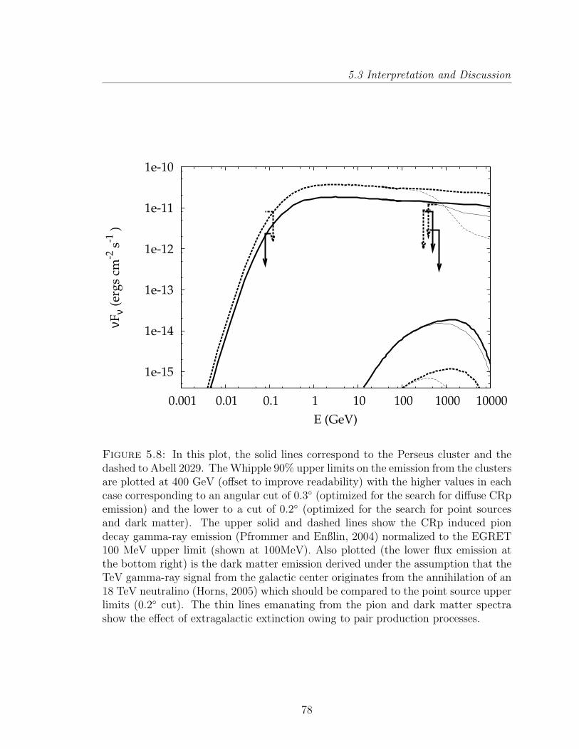
5.3 Interpretation and Discussion
1e-15
1e-14
1e-13
1e-12
1e-11
1e-10
0.001 0.01 0.1 1 10 100 1000 10000
νFν
(erg
s cm
-2 s
-1 )
E (GeV)
Figure 5.8: In this plot, the solid lines correspond to the Perseus cluster and thedashed to Abell 2029. The Whipple 90% upper limits on the emission from the clustersare plotted at 400 GeV (offset to improve readability) with the higher values in eachcase corresponding to an angular cut of 0.3 (optimized for the search for diffuse CRpemission) and the lower to a cut of 0.2 (optimized for the search for point sourcesand dark matter). The upper solid and dashed lines show the CRp induced piondecay gamma-ray emission (Pfrommer and Enßlin, 2004) normalized to the EGRET100 MeV upper limit (shown at 100MeV). Also plotted (the lower flux emission atthe bottom right) is the dark matter emission derived under the assumption that theTeV gamma-ray signal from the galactic center originates from the annihilation of an18 TeV neutralino (Horns, 2005) which should be compared to the point source upperlimits (0.2 cut). The thin lines emanating from the pion and dark matter spectrashow the effect of extragalactic extinction owing to pair production processes.
78

5.3 Interpretation and Discussion
halo (Bergstrom et al., 1998) with ρ ∝ (r/rs(1+ r/rs)2)−1, virial radius rs ' 290 kpc,
a halo mass of 4× 10¹⁴, a distance of 75 Mpc and an NFW concentration parameter
of c ' 4. It turns out that the best sensitivity (signal to background noise ratio) is
obtained if we use the same radial cut, θ = 0.3, as for the search for point sources
(reducing background from misidentified CR air showers) with the result being that
the expected dark matter signal lies two orders of magnitude or more below our upper
limits. We will not see dark matter emission even if all of the TeV galactic center
emission is dark matter in origin. Thus, we do not provide any new constraints on
TeV galactic center emission. Secondly, our calculations show that the most promising
region to observe dark matter is the galactic center.
Though we did not detect significant TeV gamma rays from these two clusters of
galaxies, we are able to determine two different types of upper limits on the emission:
from point sources within the cluster and upper limits on the extended emission. Long
duration observations with the more sensitive TeV telescopes VERITAS, H.E.S.S.,
MAGIC, and CANGAROO III and the GeV telescope GLAST will be critical for
determining whether cluster are emitters of high energy gamma rays (See Chapter
7).
79

Chapter 6
Detector Development
Cadmium Zinc Telluride (CZT) has emerged as the detector material of choice for
X-rays in the energy range from 10 keV to ∼ 1 MeV. CZT is a high Z semiconductor
which can be produced in thick (∼ 1 ′′) crystals that provide good stopping power and
energy resolution without the need for cryogenic cooling. Compared to scintillator
detectors, CZT detectors achieve a somewhat better energy resolution (1-2% FWHM
at 662 keV, compared to 10% for CsI and 3% for LaBr3) and at the same time much
better spatial resolutions (sub-mm compared to mm-cm for scintillators). CZT has
the advantage of higher Z over Si (the mean Z of CZT is 50 while Si is 14) and does
not have to be cooled like Ge. This provides a tremendous possibility to observe the
universe in the > 10keV energy range that has not been studied in depth.
80
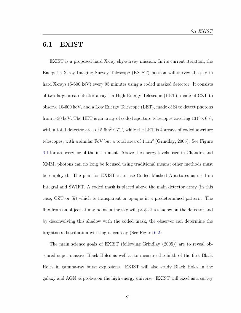
6.1 EXIST
6.1 EXIST
EXIST is a proposed hard X-ray sky-survey mission. In its current iteration, the
Energetic X-ray Imaging Survey Telescope (EXIST) mission will survey the sky in
hard X-rays (5-600 keV) every 95 minutes using a coded masked detector. It consists
of two large area detector arrays: a High Energy Telescope (HET), made of CZT to
observe 10-600 keV, and a Low Energy Telescope (LET), made of Si to detect photons
from 5-30 keV. The HET is an array of coded aperture telescopes covering 131×65,
with a total detector area of 5.6m2 CZT, while the LET is 4 arrays of coded aperture
telescopes, with a similar FoV but a total area of 1.1m2 (Grindlay, 2005). See Figure
6.1 for an overview of the instrument. Above the energy levels used in Chandra and
XMM, photons can no long be focused using traditional means; other methods must
be employed. The plan for EXIST is to use Coded Masked Apertures as used on
Integral and SWIFT. A coded mask is placed above the main detector array (in this
case, CZT or Si) which is transparent or opaque in a predetermined pattern. The
flux from an object at any point in the sky will project a shadow on the detector and
by deconvolving this shadow with the coded mask, the observer can determine the
brightness distribution with high accuracy (See Figure 6.2).
The main science goals of EXIST (following Grindlay (2005)) are to reveal ob-
scured super massive Black Holes as well as to measure the birth of the first Black
Holes in gamma-ray burst explosions. EXIST will also study Black Holes in the
galaxy and AGN as probes on the high energy universe. EXIST will excel as a survey
81
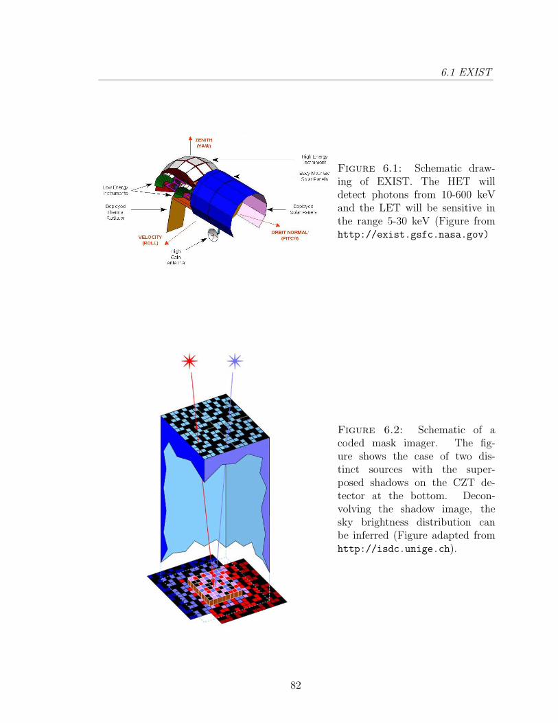
6.1 EXIST
Figure 6.1: Schematic draw-ing of EXIST. The HET willdetect photons from 10-600 keVand the LET will be sensitive inthe range 5-30 keV (Figure fromhttp://exist.gsfc.nasa.gov)
Figure 6.2: Schematic of acoded mask imager. The fig-ure shows the case of two dis-tinct sources with the super-posed shadows on the CZT de-tector at the bottom. Decon-volving the shadow image, thesky brightness distribution canbe inferred (Figure adapted fromhttp://isdc.unige.ch).
82

6.2 Equipment
instrument but will need a detector area of 6m2 of CZT whose properties are well
known.
The chapter details results from testing standard IMARAD detectors similar to
those which might be used on EXIST with a time resolved readout (Sections 6.2 and
6.3), which allowed me to investigate various ways to correct the anode signals for the
depth of the primary interaction. I developed a simplified detector model to compare
the measured signals with simulations (Section 6.5).
6.2 Equipment
The CZT crystals used here were produced by IMARAD1 using the modified
high-pressure Bridgeman growth technique. The 2 cm x 2 cm x 0.5 cm detectors were
contacted with a single Indium cathode and 8 × 8 1.6 mm square Indium pixels at
a 2.5 mm pitch at the production facility. Li et al. (2001), Hong et al. (2004) and
Narita et al. (2000, 1999) previously studied detectors from IMARAD. The cathode
channel plus three centrally located anode pixels were connected through electronics
with an analog bandwidth of 100 MHz, similar to that described by Matteson et al.
(2003), which measures the drift time of electrons in the detector to a resolution of
10 ns. Sixteen other pixels were attached to a pulse-height measuring ASIC.2 All
of the electronics were designed for low noise, making use of batteries for power and
1 IMARAD Imaging Systems, Ltd., RabinPark, 10 Plaut Street, Rehovot, ISRAEL
2 eVProducts, 373 Saxonburg Boulevard, Saxonburg, PA, 16056
83
6.3 Measurements
high-voltage, as well as cooled external FETS and ground isolation. The signals from
the 100 MHz and ASIC electronics were digitized by a 500 MHz oscilloscope and
Pulse Height Analysis PC board respectively. See Appendix D for more information
on the digital acquisition system.
6.3 Measurements
Cs137 produces an X-ray line at 662 keV and was used to produce interactions
such as those seen in Figure 6.3 within the detector by irradiating the CZT from the
cathode side. Since this is such a high energy source, most of the photons produced
do not interact with the CZT, but those that do are to first order homogeneously
distributed within the detector. When a photon interacts with the detector it pro-
duces an electron-hole cloud. Since the detector is biased at -500 V on the cathode
side with the pixels held at ground, the electrons will drift towards the pixels with
an almost constant velocity according to
~V (~x) = µ~E(~x) (6.1)
where µ is the electron mobility. The holes are trapped quickly and contribute little
to the induced signal. To determine the signal on any particular contact within the
detector, one must compute the weighting potential for that contact. This is done by
setting the voltage contact under consideration to one while holding all of the other
contacts at ground and computing the electric potential throughout the detector.
Once this is known, the induced current due to an electric charge moving within the
84

6.4 Cs137 Spectra
detector is given by
I = evφ(~x) (6.2)
where e is the charge. The holes do not contribute to this signal and the weighting
potential has a steep gradient directly in front of the pixels causing the greatest signal
to be induced shortly before they reach the pixels. This “small pixel effect” (Barret
et al., 1995) is seen in Figure 6.3 by a peak in the anode current toward the end of
the pulse. The small pixel effect is beneficial because we can accurately measure the
drift time of the electrons as well as neglect the influence of the holes. During their
drift, some electrons are trapped which can be seen in this figure by an exponential
decrease in the cathode current (quantified by the trapping time τ).
6.4 Cs137 Spectra
From data as shown in Figure 6.3, we determined the drift time of the electron
cloud in the detector by measuring the pulse time and the amplitudes of the anode
and cathode pulses. The drift time is directly correlated with the depth of interaction
in the detector (Kalemci and Matteson, 2002; He et al., 1999). We used the Cs137
source to produce several thousand events in the detector and read them with a PC.
There are numerous ways to look at the data. The first is a basic plot of the
cathode charge versus the charge induced on an anode pixel (Figure 6.4). The 662
keV photo-effect events produce a clearly recognizable arc. These data can also be
histogrammed to directly see the photo-peak (Figure 6.5). The photo-peak has a
85

6.4 Cs137 Spectra
Figure 6.3: This figure shows an electronic pulse produced when an X-ray photoninteracts with the detector. The upper panel shows the signal on the anode pixelwhile the bottom shows the cathode. In both plots the solid line is proportionalto the charge induced while the dashed line is the time derivative of that charge(current). By demarking the beginning and end of the anode pulse (the solid lines),one can determine the drift time of the electron cloud within the detector. The sharpincrease in current toward the end of the pulse is indicative of the small pixel effect,while the slow decrease in the current on the cathode shows some electron trapping.
86
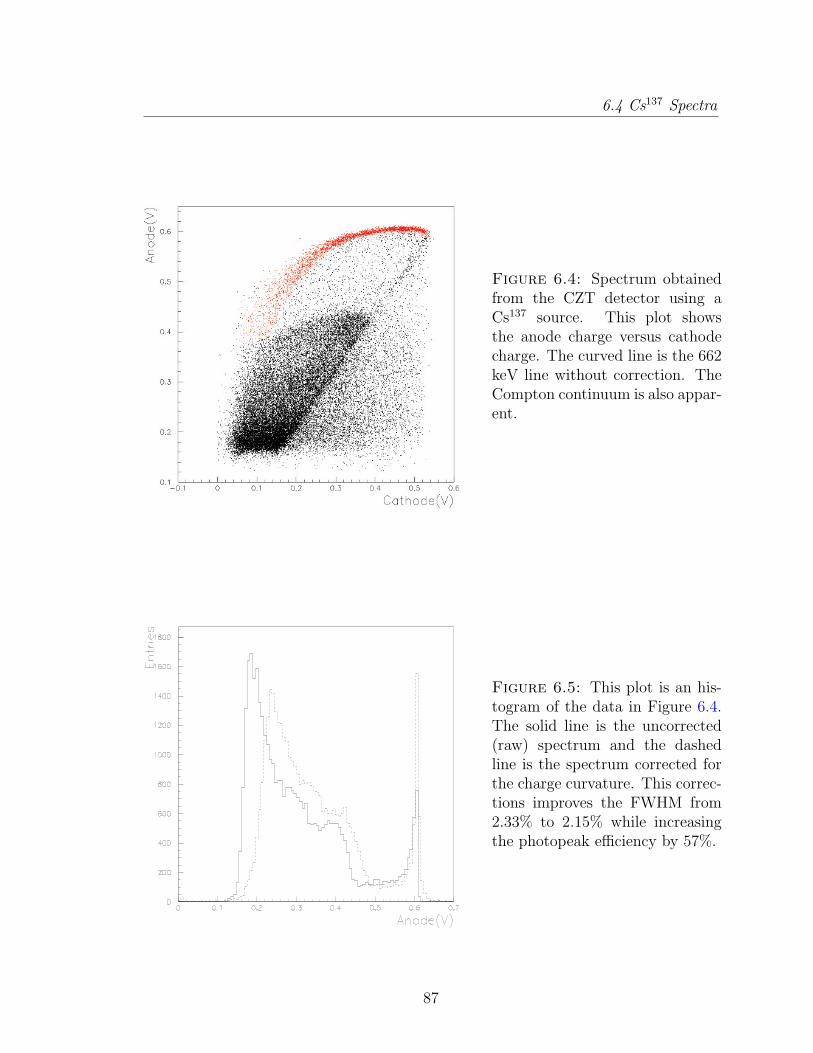
6.4 Cs137 Spectra
Figure 6.4: Spectrum obtainedfrom the CZT detector using aCs137 source. This plot showsthe anode charge versus cathodecharge. The curved line is the 662keV line without correction. TheCompton continuum is also appar-ent.
Figure 6.5: This plot is an his-togram of the data in Figure 6.4.The solid line is the uncorrected(raw) spectrum and the dashedline is the spectrum corrected forthe charge curvature. This correc-tions improves the FWHM from2.33% to 2.15% while increasingthe photopeak efficiency by 57%.
87
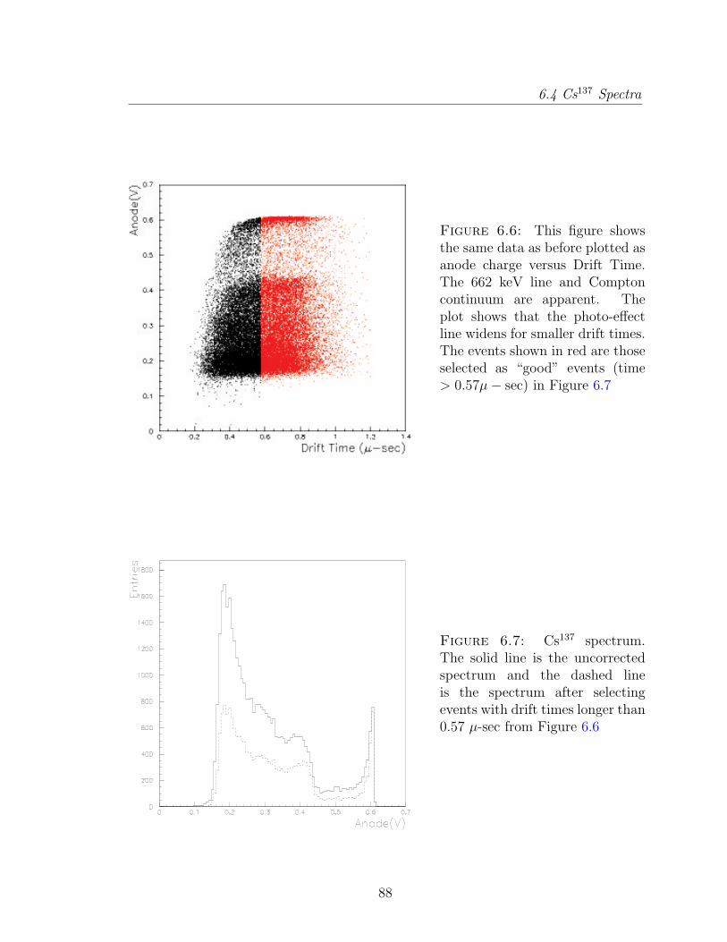
6.4 Cs137 Spectra
Figure 6.6: This figure showsthe same data as before plotted asanode charge versus Drift Time.The 662 keV line and Comptoncontinuum are apparent. Theplot shows that the photo-effectline widens for smaller drift times.The events shown in red are thoseselected as “good” events (time> 0.57µ− sec) in Figure 6.7
Figure 6.7: Cs137 spectrum.The solid line is the uncorrectedspectrum and the dashed lineis the spectrum after selectingevents with drift times longer than0.57 µ-sec from Figure 6.6
88

6.5 Simulations and Comparison to Experimental Results
FWHM of 2.33% before any type of correction. Correcting for the curvature or depth
of interaction in Figure 6.4 improves the energy resolution to 2.15% and increases
the photo-peak efficiency by 57%, which is apparent by looking at the dashed line in
Figure 6.5. Hong et al. (2004) reported similar improvements. We estimate that the
actual energy resolution is 1.8% (1.6% after correction) by subtracting the electronic
resolution in quadrature.
These same data are plotted in Figure 6.6 as the anode amplitude versus the drift
time. The photo-peak is still obvious, but there is no clear correlation correction. One
can see that the photo-peak becomes more spread out for short drift times. Thus, only
using events with drift times larger than 0.57µ−sec improves the energy resolution
from 2.33% to 2.12% (1.5% after subtracting electronic noise), but the photo-peak
efficiency decreases by 14% (see Figure 6.7).
6.5 Simulations and Comparison to Experimental
Results
I created a simulation based on a two-dimensional model to better understand the
underlying processes. I tuned the model to match the standard IMARAD detector by
setting the pixel widths to be the same but allowing for a larger pixel pitch to mimic
the 3-D geometry. I used a commercial semiconductor device simulator package called
ATLAS3 to determine the weighting potential for each pixel and the electric field
3 SILVACO International, Inc., 4701 Patrick Henry Drive, Building 2, Santa Clara, CA95054
89
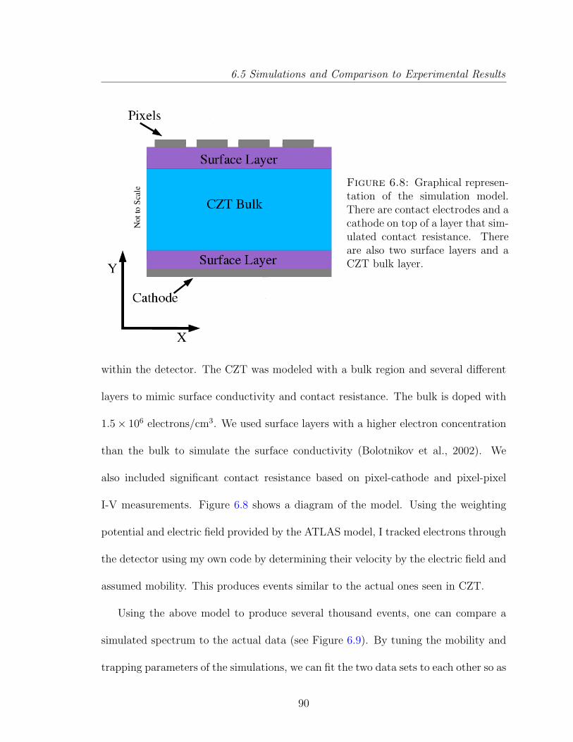
6.5 Simulations and Comparison to Experimental Results
Figure 6.8: Graphical represen-tation of the simulation model.There are contact electrodes and acathode on top of a layer that sim-ulated contact resistance. Thereare also two surface layers and aCZT bulk layer.
within the detector. The CZT was modeled with a bulk region and several different
layers to mimic surface conductivity and contact resistance. The bulk is doped with
1.5× 10⁶ electrons/cm3. We used surface layers with a higher electron concentration
than the bulk to simulate the surface conductivity (Bolotnikov et al., 2002). We
also included significant contact resistance based on pixel-cathode and pixel-pixel
I-V measurements. Figure 6.8 shows a diagram of the model. Using the weighting
potential and electric field provided by the ATLAS model, I tracked electrons through
the detector using my own code by determining their velocity by the electric field and
assumed mobility. This produces events similar to the actual ones seen in CZT.
Using the above model to produce several thousand events, one can compare a
simulated spectrum to the actual data (see Figure 6.9). By tuning the mobility and
trapping parameters of the simulations, we can fit the two data sets to each other so as
90

6.5 Simulations and Comparison to Experimental Results
Figure 6.9: Comparison of sim-ulated and experimental data.Events at long-drift times are sim-ulated well while events at short-drift times are not. We sus-pect that some of these eventsare occurring between pixels andthat holes are playing an impor-tant part. While there are onlyphoto-effect events in the simula-tions, the real data shows also theCompton continuum.
to optimize the agreement between the simulation and the data. The electron mobility
is directly shown by the longest drift times, where the trapping is constrained by the
slope of the photo-peak because longer drift time events will produce less charge due
to the charge loss. We find that the simulation deviates from the data in the region
of short drift times which is most likely due to only modeling two dimension and
by the neglecting of holes (see Figure 6.10). This indicates that the electric field as
well as the weighting potential are not simulated correctly between pixels. According
to Jung et al. (2005) the holes become important at short drift times. There are
also model deficiencies in the contact properties and surface regions. Based on these
simulations µ equals 900 cm2V−1s−1 and τ equals 1.9 µ-sec. Previous studies of
IMARAD detectors have shown similar results (Li et al., 2001) but depend strongly
on the assumed contact resistance.
A very powerful tool with the simulations is that you know exactly where in the
detector an interaction occurs. Figure 6.10 presents the charge induced on the anode
91
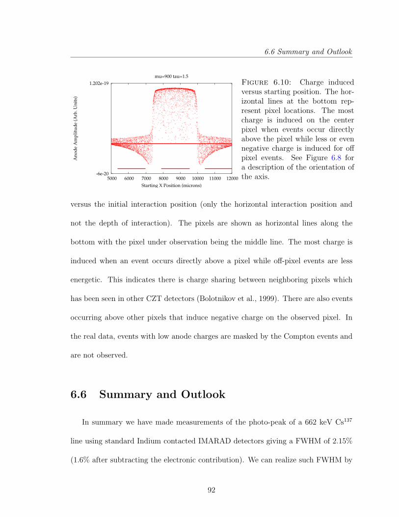
6.6 Summary and Outlook
-6e-20
1.202e-19
5000 6000 7000 8000 9000 10000 11000 12000
An
od
e A
mp
litu
de
(Arb
. Un
its)
Starting X Position (microns)
mu=900 tau=1.5
Figure 6.10: Charge inducedversus starting position. The hor-izontal lines at the bottom rep-resent pixel locations. The mostcharge is induced on the centerpixel when events occur directlyabove the pixel while less or evennegative charge is induced for offpixel events. See Figure 6.8 fora description of the orientation ofthe axis.
versus the initial interaction position (only the horizontal interaction position and
not the depth of interaction). The pixels are shown as horizontal lines along the
bottom with the pixel under observation being the middle line. The most charge is
induced when an event occurs directly above a pixel while off-pixel events are less
energetic. This indicates there is charge sharing between neighboring pixels which
has been seen in other CZT detectors (Bolotnikov et al., 1999). There are also events
occurring above other pixels that induce negative charge on the observed pixel. In
the real data, events with low anode charges are masked by the Compton events and
are not observed.
6.6 Summary and Outlook
In summary we have made measurements of the photo-peak of a 662 keV Cs137
line using standard Indium contacted IMARAD detectors giving a FWHM of 2.15%
(1.6% after subtracting the electronic contribution). We can realize such FWHM by
92
6.6 Summary and Outlook
correcting for the depth of interaction with the help of the anode to cathode charge
ratio. One of the limiting factors to resolution is the presence of leakage current at high
voltages and the determination of this effect is very important (see Appendix C.These
detectors are substantially less expensive than standard high-pressure Bridgman CZT
and are thus extremely promising for experiments requiring large detector areas such
as EXIST or other such instruments (see Chapter 7).
93

Chapter 7
Conclusions
Galaxy clusters are the largest and most massive gravitationally bound systems
in the universe. In this thesis, I reported on observations of three clusters; 3C 129,
Perseus and Abell 2029. The observations of the three clusters can be divided into two
distinct classes: X-ray observations of 3C 129 and TeV observations of the Perseus
and Abell 2029 clusters. Galaxy clusters are bright X-ray sources due to the thermal
emission of the hot ICM and may be emitters of TeV gamma rays from non-thermal
hadrons accelerated by shocks, galactic winds or AGN. The observations presented
here had two different goals. In the case of 3C 129 it was to verify and expand on
the Chandra results reported on by Krawczynski et al. (2003), specifically to look for
deficits in the X-ray surface brightness along the radio tail and to search for a possible
diffuse excess in the region in front of the radio tail. The TeV observations had a
different task in that VHE gamma rays had previously not yet been seen from clusters
and our goal was to search for such emission. The detection of TeV gamma rays from
94
clusters would allow us to constrain the energy density of non-thermal particles in
clusters.
Using the XMM-Newton X-ray observatory, we observed the prototypical head-tail
radio galaxy 3C 129, first searching for deficits due to the non-thermal radio plasma
displacing the thermal ICM. We report an upper limit of 1.5% on the fractional
deficit within the radio jet which is much smaller than the expected 10% change.
This suggests that there is some mixing of the thermal and non-thermal plasmas. If
the deficit was on the order of what we suspect, we could have computed the plasma
volume filling factor and further constrain the magnetic energy density of the plasma.
Krawczynski et al. (2003) saw marginal evidence for extended emission in front of the
radio galaxy at the head of the jet which would indicate the presence of a compressed
higher density plasma. Since the angular resolution of XMM is not good enough to
resolve a feature of this size, I fit a power-law to a larger region that includes both
the core and the extended feature. This shows that there is 62% more flux from the
larger XMM region than the Chandra point source, indicating that there is some type
of extended emission. However, the XMM excess is smaller than expected from the
tentative Chandra detection. Unfortunately, we cannot further localize the excess
with XMM.
Using the Whipple 10 m Cherenkov telescope, we searched for TeV gamma-ray
emission from the Perseus and Abell 2029 clusters. The first task was a point source
search using the standard parameterization technique which resulted in the produc-
tion of an upper limit map (Figures 5.6 and 5.7). There were no discernible VHE
95
7.1 Future Cluster Observations
point sources within either of the clusters. We reported upper limits at the locations
of several point sources within the clusters, including the CD galaxies (see Table 5.3).
Finally, several authors have suggested that there would be diffuse VHE emission from
clusters of galaxies due to a population of non-thermal particles. We assumed that
the non-thermal particles mimic the distribution of the thermal ICM. Based on this
assumption, we looked for extended emission at several radial distances for Perseus
and Abell 2029 and compared these with model calculations. For the Perseus cluster,
our results imply that the cosmic ray proton energy density is less than 7.9% of the
thermal energy density if the CRp spectrum follows a power-law with spectral index
of -2.1 all the way to TeV energies. TeV gamma-rays might also originate from dark
matter, so we compared our result to a possible dark matter annihilation spectrum.
Unfortunately, due to the distance and mass of these objects, it lies several orders of
magnitude below the sensitivity of the Whipple telescope. A paper describing these
results is in press in the Astrophysical Journal (Perkins et al., 2006).
7.1 Future Cluster Observations
Chandra and XMM reached the best performance that can be achieved with a
Wolter mirror design and Si CCDs. Chandra, with its < 0.5 arcsecond resolution
and XMM with its large detector area are arguably the best that the field of Wolter
mirrors and silicon CCDs has to offer. Designing observatories that can give com-
plementary information to that obtained with Chandra and XMM with an equal or
96
7.1 Future Cluster Observations
smaller amount of resources requires different technology. In the following I will de-
scribe proposed and under construction experiments that are expected to have an
impact on the study of non-thermal emission from galaxy clusters.
7.1.1 NuSTAR and GLAST
The satellite-borne Nuclear Spectroscopic Telescope Array (NuSTAR, and later
the Constellation-X mission, see Hornschemeier et al. (2005)) would extend the capa-
bilities of Chandra into the hard X-ray band (6 keV up to 80 keV) by using grazing
incidence mirrors to focus photons with a focal length of ten meters together with
2 mm thick CZT detectors (Harrison et. al., 2004). This would be very useful for
cluster research. Figure 7.1 compares the effective area of NuSTAR with current
observatories. The main science objectives of NuSTAR are similar to EXIST and
include a Black Hole survey (looking for obscured black holes). It will also be very
useful for pointed observations of clusters, Super Nova Remnants, and AGN. Using
the RXTE satellite, Gruber and Rephaeli (2002) reported tentative evidence of non-
thermal emission from Abell 2319 at the very end of the thermal bremsstrahlung
emission above 10 keV. If there is such emission, then NuSTAR, with a sensitivity
that is one order of magnitude higher than that of RXTE and extends all the way
to 80 keV, would definitely detect it. NuSTAR might probe the region between the
thermal and the non-thermal.
GLAST is another satellite-borne instrument with a viable detection range be-
tween the ground based IACTs and the current X-ray missions (Ritz et al., 2005).
97

7.2 VERITAS and H.E.S.S.
Figure 7.1: The effective areaof the proposed NuSTAR mis-sion using CZT detectors. Nu-STAR would be ideal for detect-ing non-thermal tails in the ICMX-ray energy spectra (Figure fromhttp://www.nustar.caltech.edu).
GLAST is a Silicon pair tracker experiment that will have an energy range from 30
MeV to 300 GeV and will be able to locate sources with an accuracy of 30 arcseconds
for the very strongest sources to tens of arcminutes for weak sources. GLAST, being
a wide field of view instrument, would take one to two years to achieve the sensitivity
needed for these clusters (see Figure 7.2).
7.2 VERITAS and H.E.S.S.
The Very Energetic Radiation Imaging Telescope Array System (VERITAS) is an
array of four IACTs currently in construction in Amado, Arizona, near the current
site of the Whipple 10 m system (Falcone et al., 2005). Two of the four telescopes are
in operation as of the writing of this while the final two are scheduled to be completed
in December 2006. The H.E.S.S. (High Energy Stereoscopic System) collaboration
has been operating an array of four telescopes in Namibia since December of 2003
(Benbow et. al., 2005). There are several benefits to an array of IACTs over a
98
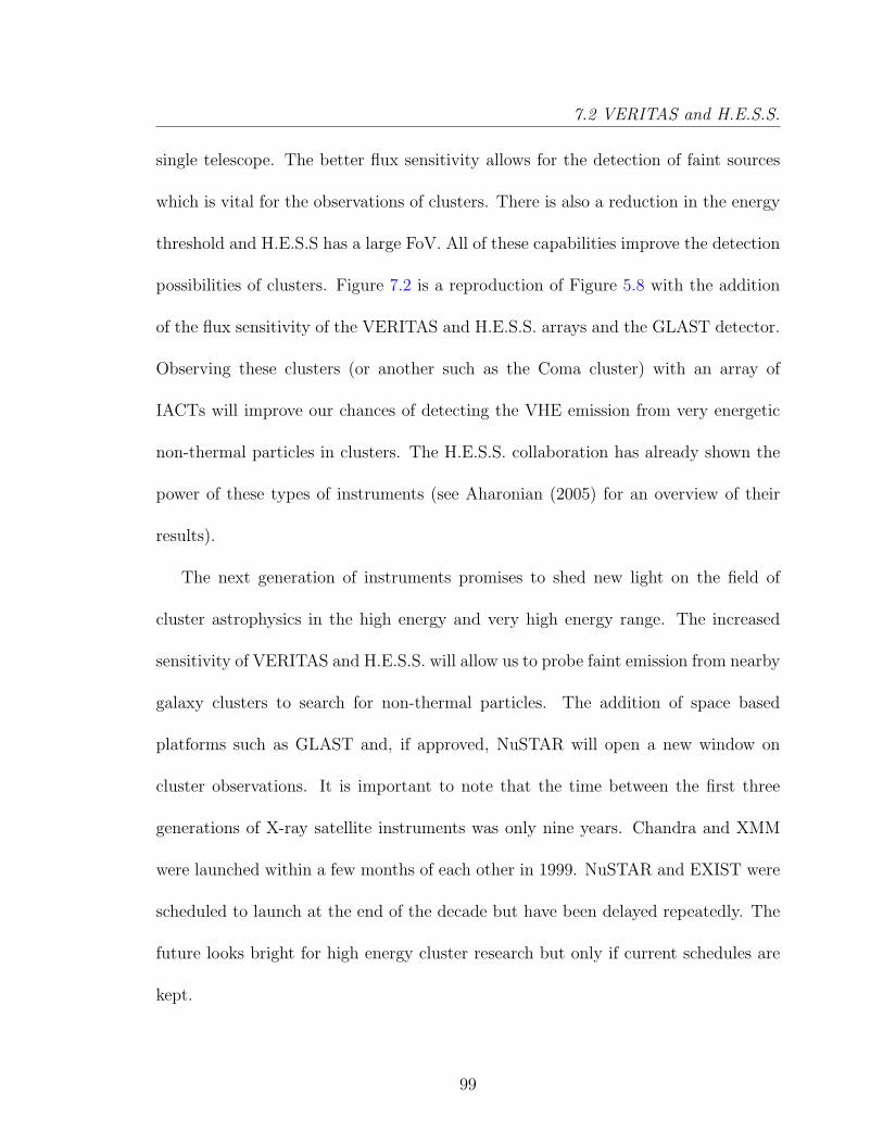
7.2 VERITAS and H.E.S.S.
single telescope. The better flux sensitivity allows for the detection of faint sources
which is vital for the observations of clusters. There is also a reduction in the energy
threshold and H.E.S.S has a large FoV. All of these capabilities improve the detection
possibilities of clusters. Figure 7.2 is a reproduction of Figure 5.8 with the addition
of the flux sensitivity of the VERITAS and H.E.S.S. arrays and the GLAST detector.
Observing these clusters (or another such as the Coma cluster) with an array of
IACTs will improve our chances of detecting the VHE emission from very energetic
non-thermal particles in clusters. The H.E.S.S. collaboration has already shown the
power of these types of instruments (see Aharonian (2005) for an overview of their
results).
The next generation of instruments promises to shed new light on the field of
cluster astrophysics in the high energy and very high energy range. The increased
sensitivity of VERITAS and H.E.S.S. will allow us to probe faint emission from nearby
galaxy clusters to search for non-thermal particles. The addition of space based
platforms such as GLAST and, if approved, NuSTAR will open a new window on
cluster observations. It is important to note that the time between the first three
generations of X-ray satellite instruments was only nine years. Chandra and XMM
were launched within a few months of each other in 1999. NuSTAR and EXIST were
scheduled to launch at the end of the decade but have been delayed repeatedly. The
future looks bright for high energy cluster research but only if current schedules are
kept.
99
7.2 VERITAS and H.E.S.S.
1e-15
1e-14
1e-13
1e-12
1e-11
1e-10
0.001 0.01 0.1 1 10 100 1000 10000
νFν (
ergs
cm-2
s-1 )
E (GeV)
Veritas/H.E.S.S.GLAST
Figure 7.2: This plot is a duplicate of Figure 5.8 with the addition of the predictedsensitivity of the VERITAS or H.E.S.S. arrays (for a 50 hr observation) shown as thedashed-dotted lines and the sensitivity of GLAST (for a 2 year observation) as thedouble dotted lines. As a reminder, the solid lines correspond to the Perseus clusterand the dashed to Abell 2029. See Figure 5.8 for more details on the upper limitsand models.
100
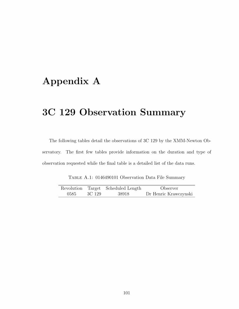
Appendix A
3C 129 Observation Summary
The following tables detail the observations of 3C 129 by the XMM-Newton Ob-
servatory. The first few tables provide information on the duration and type of
observation requested while the final table is a detailed list of the data runs.
Table A.1: 0146490101 Observation Data File Summary
Revolution Target Scheduled Length Observer0585 3C 129 38918 Dr Henric Krawczynski
101
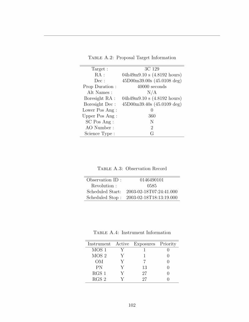
Table A.2: Proposal Target Information
Target : 3C 129RA : 04h49m9.10 s (4.8192 hours)Dec : 45D00m39.00s (45.0108 deg)
Prop Duration : 40000 secondsAlt Names : N/A
Boresight RA : 04h49m9.10 s (4.8192 hours)Boresight Dec : 45D00m39.40s (45.0109 deg)Lower Pos Ang : 0Upper Pos Ang : 360
SC Pos Ang : NAO Number : 2Science Type : G
Table A.3: Observation Record
Observation ID : 0146490101Revolution : 0585
Scheduled Start: 2003-02-18T07:24:41.000Scheduled Stop : 2003-02-18T18:13:19.000
Table A.4: Instrument Information
Instrument Active Exposures PriorityMOS 1 Y 1 0MOS 2 Y 1 0
OM Y 7 0PN Y 13 0
RGS 1 Y 27 0RGS 2 Y 27 0
102
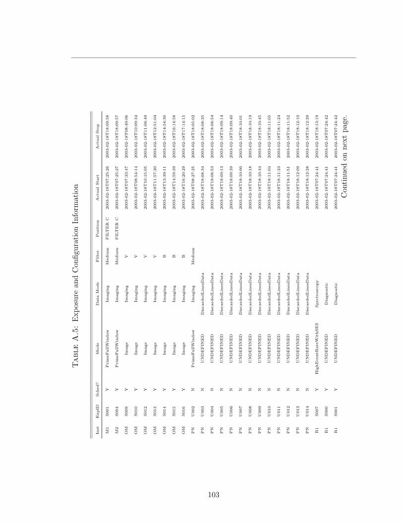
Table
A.5
:E
xpos
ure
and
Con
figu
rati
onIn
form
atio
n
Inst
ExpID
Sched?
Mode
Data
Mode
Filte
rPosi
tion
Actu
alSta
rtA
ctu
alSto
p
M1
S001
YPri
meFullW
indow
Imagin
gM
ediu
mFIL
TER
C2003-0
2-1
8T
07:2
5:2
62003-0
2-1
8T
18:0
9:5
8
M2
S004
YPri
meFullW
indow
Imagin
gM
ediu
mFIL
TER
C2003-0
2-1
8T
07:2
5:2
72003-0
2-1
8T
18:0
9:5
7
OM
S009
YIm
age
Imagin
gV
2003-0
2-1
8T
07:3
3:4
72003-0
2-1
8T
08:4
9:0
6
OM
S010
YIm
age
Imagin
gV
2003-0
2-1
8T
08:5
4:1
42003-0
2-1
8T
10:0
9:3
4
OM
S012
YIm
age
Imagin
gV
2003-0
2-1
8T
10:1
5:0
52003-0
2-1
8T
11:0
8:4
9
OM
S013
YIm
age
Imagin
gV
2003-0
2-1
8T
11:5
7:2
02003-0
2-1
8T
12:5
1:0
4
OM
S014
YIm
age
Imagin
gB
2003-0
2-1
8T
13:3
9:1
12003-0
2-1
8T
14:5
4:3
0
OM
S015
YIm
age
Imagin
gB
2003-0
2-1
8T
14:5
9:3
92003-0
2-1
8T
16:1
4:5
8
OM
S016
YIm
age
Imagin
gB
2003-0
2-1
8T
16:2
0:2
92003-0
2-1
8T
17:1
4:1
5
PN
U002
NPri
meFullW
indow
Imagin
gM
ediu
m2003-0
2-1
8T
08:2
7:2
52003-0
2-1
8T
18:0
5:0
2
PN
U003
NU
ND
EFIN
ED
Dis
card
edLin
esD
ata
2003-0
2-1
8T
18:0
8:3
42003-0
2-1
8T
18:0
8:3
5
PN
U004
NU
ND
EFIN
ED
Dis
card
edLin
esD
ata
2003-0
2-1
8T
18:0
8:5
32003-0
2-1
8T
18:0
8:5
4
PN
U005
NU
ND
EFIN
ED
Dis
card
edLin
esD
ata
2003-0
2-1
8T
18:0
9:1
32003-0
2-1
8T
18:0
9:1
4
PN
U006
NU
ND
EFIN
ED
Dis
card
edLin
esD
ata
2003-0
2-1
8T
18:0
9:3
92003-0
2-1
8T
18:0
9:4
0
PN
U007
NU
ND
EFIN
ED
Dis
card
edLin
esD
ata
2003-0
2-1
8T
18:1
0:0
02003-0
2-1
8T
18:1
0:0
1
PN
U008
NU
ND
EFIN
ED
Dis
card
edLin
esD
ata
2003-0
2-1
8T
18:1
0:1
82003-0
2-1
8T
18:1
0:1
9
PN
U009
NU
ND
EFIN
ED
Dis
card
edLin
esD
ata
2003-0
2-1
8T
18:1
0:4
42003-0
2-1
8T
18:1
0:4
5
PN
U010
NU
ND
EFIN
ED
Dis
card
edLin
esD
ata
2003-0
2-1
8T
18:1
1:0
42003-0
2-1
8T
18:1
1:0
5
PN
U011
NU
ND
EFIN
ED
Dis
card
edLin
esD
ata
2003-0
2-1
8T
18:1
1:2
32003-0
2-1
8T
18:1
1:2
4
PN
U012
NU
ND
EFIN
ED
Dis
card
edLin
esD
ata
2003-0
2-1
8T
18:1
1:5
12003-0
2-1
8T
18:1
1:5
2
PN
U013
NU
ND
EFIN
ED
Dis
card
edLin
esD
ata
2003-0
2-1
8T
18:1
2:0
92003-0
2-1
8T
18:1
2:1
0
PN
U014
NU
ND
EFIN
ED
Dis
card
edLin
esD
ata
2003-0
2-1
8T
18:1
2:2
82003-0
2-1
8T
18:1
2:2
9
R1
S007
YH
ighEventR
ate
Wit
hSES
Spectr
osc
opy
2003-0
2-1
8T
07:2
4:4
12003-0
2-1
8T
18:1
3:1
9
R1
S900
YU
ND
EFIN
ED
Dia
gnost
ic2003-0
2-1
8T
07:2
4:4
12003-0
2-1
8T
07:2
4:4
2
R1
S901
YU
ND
EFIN
ED
Dia
gnost
ic2003-0
2-1
8T
07:2
4:4
12003-0
2-1
8T
07:2
4:4
2
Con
tinued
onnex
tpag
e.
103

Inst
ExpID
Sched?
Mode
Data
Mode
Filte
rPosi
tion
Actu
alSta
rtA
ctu
alSto
p
R1
S902
YU
ND
EFIN
ED
Dia
gnost
ic2003-0
2-1
8T
07:2
4:4
12003-0
2-1
8T
07:2
4:4
2
R1
S903
YU
ND
EFIN
ED
Dia
gnost
ic2003-0
2-1
8T
07:2
4:4
12003-0
2-1
8T
07:2
4:4
2
R1
S904
YU
ND
EFIN
ED
Dia
gnost
ic2003-0
2-1
8T
07:2
4:4
12003-0
2-1
8T
07:2
4:4
2
R1
S905
YU
ND
EFIN
ED
Dia
gnost
ic2003-0
2-1
8T
07:2
4:4
12003-0
2-1
8T
07:2
4:4
2
R1
S906
YU
ND
EFIN
ED
Dia
gnost
ic2003-0
2-1
8T
07:2
4:4
12003-0
2-1
8T
07:2
4:4
2
R1
S907
YU
ND
EFIN
ED
Dia
gnost
ic2003-0
2-1
8T
07:2
4:4
12003-0
2-1
8T
07:2
4:4
2
R1
S908
YU
ND
EFIN
ED
Dia
gnost
ic2003-0
2-1
8T
07:2
4:4
12003-0
2-1
8T
07:2
4:4
2
R1
S909
YU
ND
EFIN
ED
Dia
gnost
ic2003-0
2-1
8T
07:2
4:4
12003-0
2-1
8T
07:2
4:4
2
R1
S910
YU
ND
EFIN
ED
Dia
gnost
ic2003-0
2-1
8T
07:2
4:4
12003-0
2-1
8T
07:2
4:4
2
R1
S911
YU
ND
EFIN
ED
Dia
gnost
ic2003-0
2-1
8T
07:2
4:4
12003-0
2-1
8T
07:2
4:4
2
R1
S912
YU
ND
EFIN
ED
Dia
gnost
ic2003-0
2-1
8T
07:2
4:4
12003-0
2-1
8T
07:2
4:4
2
R1
S913
YU
ND
EFIN
ED
Dia
gnost
ic2003-0
2-1
8T
07:2
4:4
12003-0
2-1
8T
07:2
4:4
2
R1
S914
YU
ND
EFIN
ED
Dia
gnost
ic2003-0
2-1
8T
07:2
4:4
12003-0
2-1
8T
07:2
4:4
2
R1
S915
YU
ND
EFIN
ED
Dia
gnost
ic2003-0
2-1
8T
07:2
4:4
12003-0
2-1
8T
07:2
4:4
2
R1
S916
YU
ND
EFIN
ED
Dia
gnost
ic2003-0
2-1
8T
07:2
4:4
12003-0
2-1
8T
07:2
4:4
2
R1
S917
YU
ND
EFIN
ED
Dia
gnost
ic2003-0
2-1
8T
07:2
4:4
12003-0
2-1
8T
07:2
4:4
2
R1
S918
YU
ND
EFIN
ED
Dia
gnost
ic2003-0
2-1
8T
07:2
4:4
12003-0
2-1
8T
07:2
4:4
2
R1
S919
YU
ND
EFIN
ED
Dia
gnost
ic2003-0
2-1
8T
07:2
4:4
12003-0
2-1
8T
07:2
4:4
2
R1
S920
YU
ND
EFIN
ED
Dia
gnost
ic2003-0
2-1
8T
07:2
4:4
12003-0
2-1
8T
07:2
4:4
2
R1
S921
YU
ND
EFIN
ED
Dia
gnost
ic2003-0
2-1
8T
07:2
4:4
12003-0
2-1
8T
07:2
4:4
2
R1
S922
YU
ND
EFIN
ED
Dia
gnost
ic2003-0
2-1
8T
07:2
4:4
12003-0
2-1
8T
07:2
4:4
2
R1
S923
YU
ND
EFIN
ED
Dia
gnost
ic2003-0
2-1
8T
07:2
4:4
12003-0
2-1
8T
07:2
4:4
2
R1
S924
YU
ND
EFIN
ED
Dia
gnost
ic2003-0
2-1
8T
07:2
4:4
12003-0
2-1
8T
07:2
4:4
2
R1
S925
YU
ND
EFIN
ED
Dia
gnost
ic2003-0
2-1
8T
07:2
4:4
12003-0
2-1
8T
07:2
4:4
2
R2
S008
YH
ighEventR
ate
Wit
hSES
Spectr
osc
opy
2003-0
2-1
8T
07:2
4:4
12003-0
2-1
8T
18:1
3:1
5
R2
S900
YU
ND
EFIN
ED
Dia
gnost
ic2003-0
2-1
8T
07:2
4:4
12003-0
2-1
8T
07:2
4:4
2
R2
S901
YU
ND
EFIN
ED
Dia
gnost
ic2003-0
2-1
8T
07:2
4:4
12003-0
2-1
8T
07:2
4:4
2
R2
S902
YU
ND
EFIN
ED
Dia
gnost
ic2003-0
2-1
8T
07:2
4:4
12003-0
2-1
8T
07:2
4:4
2
Con
tinued
onnex
tpag
e.
104

Inst
ExpID
Sched?
Mode
Data
Mode
Filte
rPosi
tion
Actu
alSta
rtA
ctu
alSto
p
R2
S903
YU
ND
EFIN
ED
Dia
gnost
ic2003-0
2-1
8T
07:2
4:4
12003-0
2-1
8T
07:2
4:4
2
R2
S904
YU
ND
EFIN
ED
Dia
gnost
ic2003-0
2-1
8T
07:2
4:4
12003-0
2-1
8T
07:2
4:4
2
R2
S905
YU
ND
EFIN
ED
Dia
gnost
ic2003-0
2-1
8T
07:2
4:4
12003-0
2-1
8T
07:2
4:4
2
R2
S906
YU
ND
EFIN
ED
Dia
gnost
ic2003-0
2-1
8T
07:2
4:4
12003-0
2-1
8T
07:2
4:4
2
R2
S907
YU
ND
EFIN
ED
Dia
gnost
ic2003-0
2-1
8T
07:2
4:4
12003-0
2-1
8T
07:2
4:4
2
R2
S908
YU
ND
EFIN
ED
Dia
gnost
ic2003-0
2-1
8T
07:2
4:4
12003-0
2-1
8T
07:2
4:4
2
R2
S909
YU
ND
EFIN
ED
Dia
gnost
ic2003-0
2-1
8T
07:2
4:4
12003-0
2-1
8T
07:2
4:4
2
R2
S910
YU
ND
EFIN
ED
Dia
gnost
ic2003-0
2-1
8T
07:2
4:4
12003-0
2-1
8T
07:2
4:4
2
R2
S911
YU
ND
EFIN
ED
Dia
gnost
ic2003-0
2-1
8T
07:2
4:4
12003-0
2-1
8T
07:2
4:4
2
R2
S912
YU
ND
EFIN
ED
Dia
gnost
ic2003-0
2-1
8T
07:2
4:4
12003-0
2-1
8T
07:2
4:4
2
R2
S913
YU
ND
EFIN
ED
Dia
gnost
ic2003-0
2-1
8T
07:2
4:4
12003-0
2-1
8T
07:2
4:4
2
R2
S914
YU
ND
EFIN
ED
Dia
gnost
ic2003-0
2-1
8T
07:2
4:4
12003-0
2-1
8T
07:2
4:4
2
R2
S915
YU
ND
EFIN
ED
Dia
gnost
ic2003-0
2-1
8T
07:2
4:4
12003-0
2-1
8T
07:2
4:4
2
R2
S916
YU
ND
EFIN
ED
Dia
gnost
ic2003-0
2-1
8T
07:2
4:4
12003-0
2-1
8T
07:2
4:4
2
R2
S917
YU
ND
EFIN
ED
Dia
gnost
ic2003-0
2-1
8T
07:2
4:4
12003-0
2-1
8T
07:2
4:4
2
R2
S918
YU
ND
EFIN
ED
Dia
gnost
ic2003-0
2-1
8T
07:2
4:4
12003-0
2-1
8T
07:2
4:4
2
R2
S919
YU
ND
EFIN
ED
Dia
gnost
ic2003-0
2-1
8T
07:2
4:4
12003-0
2-1
8T
07:2
4:4
2
R2
S920
YU
ND
EFIN
ED
Dia
gnost
ic2003-0
2-1
8T
07:2
4:4
12003-0
2-1
8T
07:2
4:4
2
R2
S921
YU
ND
EFIN
ED
Dia
gnost
ic2003-0
2-1
8T
07:2
4:4
12003-0
2-1
8T
07:2
4:4
2
R2
S922
YU
ND
EFIN
ED
Dia
gnost
ic2003-0
2-1
8T
07:2
4:4
12003-0
2-1
8T
07:2
4:4
2
R2
S923
YU
ND
EFIN
ED
Dia
gnost
ic2003-0
2-1
8T
07:2
4:4
12003-0
2-1
8T
07:2
4:4
2
R2
S924
YU
ND
EFIN
ED
Dia
gnost
ic2003-0
2-1
8T
07:2
4:4
12003-0
2-1
8T
07:2
4:4
2
R2
S925
YU
ND
EFIN
ED
Dia
gnost
ic2003-0
2-1
8T
07:2
4:4
12003-0
2-1
8T
07:2
4:4
2
105
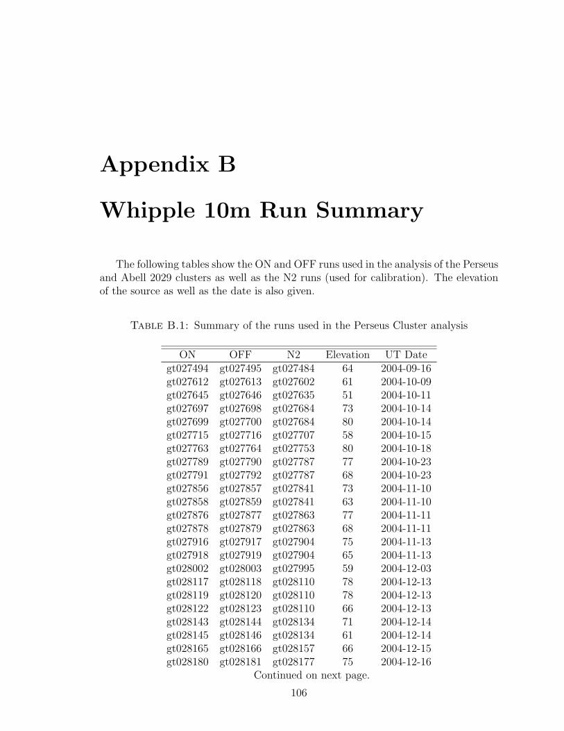
Appendix B
Whipple 10m Run Summary
The following tables show the ON and OFF runs used in the analysis of the Perseusand Abell 2029 clusters as well as the N2 runs (used for calibration). The elevationof the source as well as the date is also given.
Table B.1: Summary of the runs used in the Perseus Cluster analysis
ON OFF N2 Elevation UT Dategt027494 gt027495 gt027484 64 2004-09-16gt027612 gt027613 gt027602 61 2004-10-09gt027645 gt027646 gt027635 51 2004-10-11gt027697 gt027698 gt027684 73 2004-10-14gt027699 gt027700 gt027684 80 2004-10-14gt027715 gt027716 gt027707 58 2004-10-15gt027763 gt027764 gt027753 80 2004-10-18gt027789 gt027790 gt027787 77 2004-10-23gt027791 gt027792 gt027787 68 2004-10-23gt027856 gt027857 gt027841 73 2004-11-10gt027858 gt027859 gt027841 63 2004-11-10gt027876 gt027877 gt027863 77 2004-11-11gt027878 gt027879 gt027863 68 2004-11-11gt027916 gt027917 gt027904 75 2004-11-13gt027918 gt027919 gt027904 65 2004-11-13gt028002 gt028003 gt027995 59 2004-12-03gt028117 gt028118 gt028110 78 2004-12-13gt028119 gt028120 gt028110 78 2004-12-13gt028122 gt028123 gt028110 66 2004-12-13gt028143 gt028144 gt028134 71 2004-12-14gt028145 gt028146 gt028134 61 2004-12-14gt028165 gt028166 gt028157 66 2004-12-15gt028180 gt028181 gt028177 75 2004-12-16
Continued on next page.
106
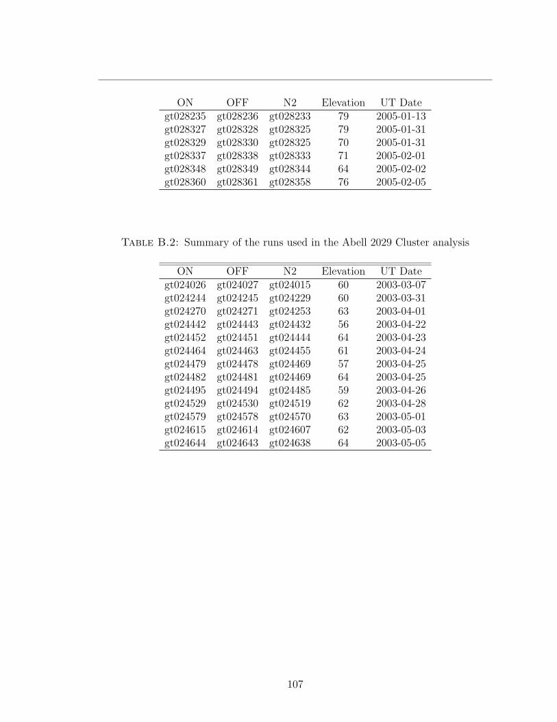
ON OFF N2 Elevation UT Dategt028235 gt028236 gt028233 79 2005-01-13gt028327 gt028328 gt028325 79 2005-01-31gt028329 gt028330 gt028325 70 2005-01-31gt028337 gt028338 gt028333 71 2005-02-01gt028348 gt028349 gt028344 64 2005-02-02gt028360 gt028361 gt028358 76 2005-02-05
Table B.2: Summary of the runs used in the Abell 2029 Cluster analysis
ON OFF N2 Elevation UT Dategt024026 gt024027 gt024015 60 2003-03-07gt024244 gt024245 gt024229 60 2003-03-31gt024270 gt024271 gt024253 63 2003-04-01gt024442 gt024443 gt024432 56 2003-04-22gt024452 gt024451 gt024444 64 2003-04-23gt024464 gt024463 gt024455 61 2003-04-24gt024479 gt024478 gt024469 57 2003-04-25gt024482 gt024481 gt024469 64 2003-04-25gt024495 gt024494 gt024485 59 2003-04-26gt024529 gt024530 gt024519 62 2003-04-28gt024579 gt024578 gt024570 63 2003-05-01gt024615 gt024614 gt024607 62 2003-05-03gt024644 gt024643 gt024638 64 2003-05-05
107

Appendix C
I-V Measurements
C.1 Standard Measurements
The goal of the standard I-V measurements is to measure the bulk leakage current
through CZT detectors. This setup allows for the automated measurement of several
pixels (currently four but could be expanded to eight or more) while ramping up the
voltage to a user specified amount. There are several safeguards in place to limit the
amount of current flowing through the detector. An example of the possible results
are given in Figure C.1. The data acquisition program has been written in LabView.1
C.1.1 Apparatus
The goal is to determine the current through the CZT (Id). See Figure C.2 for a
schematic of the setup.
VHV − Vt = IdRd and Vt = It
(1
Re
+1
Rt
)−1
(C.1)
1 National Instruments Corporation, 11500 N Mopac Expwy, Austin, TX 78759-3504
108
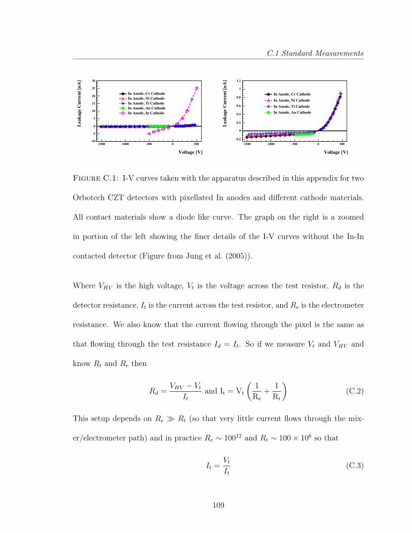
C.1 Standard Measurements
Voltage [V]
-1500 -1000 -500 0 500
Leak
age
Cur
rent
[nA
]
-10
-5
0
5
10
15
20
25
30
In Anode, Cr CathodeIn Anode, Ni CathodeIn Anode, Ti CathodeIn Anode, Au CathodeIn Anode, In Cathode
Voltage [V]
-1500 -1000 -500 0 500
Leak
age
Cur
rent
[nA
]
-0.2
0
0.2
0.4
0.6
0.8
1
1.2
In Anode, Cr CathodeIn Anode, Ni CathodeIn Anode, Ti CathodeIn Anode, Au Cathode
Figure C.1: I-V curves taken with the apparatus described in this appendix for two
Orbotech CZT detectors with pixellated In anodes and different cathode materials.
All contact materials show a diode like curve. The graph on the right is a zoomed
in portion of the left showing the finer details of the I-V curves without the In-In
contacted detector (Figure from Jung et al. (2005)).
Where VHV is the high voltage, Vt is the voltage across the test resistor, Rd is the
detector resistance, It is the current across the test resistor, and Re is the electrometer
resistance. We also know that the current flowing through the pixel is the same as
that flowing through the test resistance Id = It. So if we measure Vt and VHV and
know Rt and Re then
Rd =VHV − Vt
It
and It = Vt
(1
Re
+1
Rt
)(C.2)
This setup depends on Re Rt (so that very little current flows through the mix-
er/electrometer path) and in practice Re ∼ 10012 and Rt ∼ 100× 106 so that
It =Vt
It
(C.3)
109

C.1 Standard Measurements
Table C.1: I-V Equipment.
Part Model
Mixer Maxim DG408
Electrometer Keithley 614
DAQ NI PCI-6024E
HV Bertan 205A-03R
Rt 100 MΩ 1%
thus,
Rd =VHV − Vt
Vt
Rt (C.4)
which are all measurable or known. Table C.1 gives the models of the equipment used
and Table C.2 gives the pin out and ins for all the equipment.
C.1.2 LabView Program
Figure C.3 shows an image of the front panel of the LabView program. Figures
C.4,C.5 and C.6 show block diagrams of the LabView program (the block diagram
is the main program of the graphical programming language, LabView). All of the
possible diagrams are not shown here but the main logic of the data acquisition system
can be understood from these diagrams. The full program can be accessed by looking
at the full block diagram within the program itself on the PC attached to the I-V
setup.
110
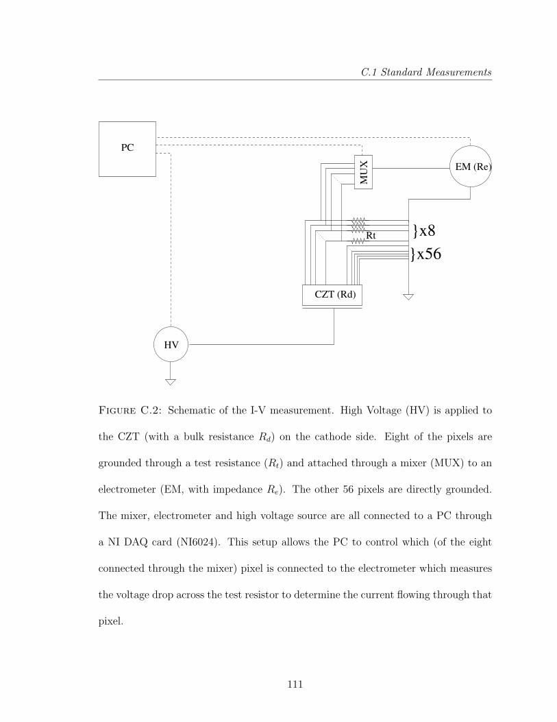
C.1 Standard Measurements
x8x56
PC
Rt
MU
X
HV
EM (Re)
CZT (Rd)
Figure C.2: Schematic of the I-V measurement. High Voltage (HV) is applied to
the CZT (with a bulk resistance Rd) on the cathode side. Eight of the pixels are
grounded through a test resistance (Rt) and attached through a mixer (MUX) to an
electrometer (EM, with impedance Re). The other 56 pixels are directly grounded.
The mixer, electrometer and high voltage source are all connected to a PC through
a NI DAQ card (NI6024). This setup allows the PC to control which (of the eight
connected through the mixer) pixel is connected to the electrometer which measures
the voltage drop across the test resistor to determine the current flowing through that
pixel.
111

C.1 Standard Measurements
Table C.2: I-V Connections.
DAQ Pin DAQ Name Equipment Pin Equipment Name
52 P0.0 MUX A0 Mixer Logic 0
17 P0.1 MUX A1 Mixer Logic 1
49 P0.2 MUX A2 Mixer Logic 2
47 P0.3 MUX EN Mixer Logic EN
68 AI 0 HV-E 0-5V Monitoring
34 AI 8 HV-C Ground
22 AO 0 HV-B 0-5V Programming
33 AI 1 E- Electrometer Negative Monitoring
66 AI 9 E+ Electrometer Positive Monitoring
112

C.1 Standard Measurements
To perform a standard measurement follow the instructions below:
• Load a detector into the current measurement apparatus being careful about
how much force you apply.
• Turn on the Electrometer, HV (must be set to rear control) and all power
supplies.
• Run the LabView program from the PC
• Visually inspect the values found on the Front Panel (C.3). Do they make
sense?
• Set the HV to a significant but low value (∼ 100V ) and inspect the values again.
Do they still make sense?
• Set the HV to 0 and switch to a different channel and raise the voltage again
and again visually inspect the values.
• If any of these tests fail, something is wrong and we need to troubleshoot a bit.
• Now, run a constant voltage test to see what the settling time is. Once you do
this, set the settling time for the standard run.
• Do a standard run - if you set the top voltage too high, the current might go
beyond the set-point and the run will cancel. If this happens, just set it lower
and run it again.
113
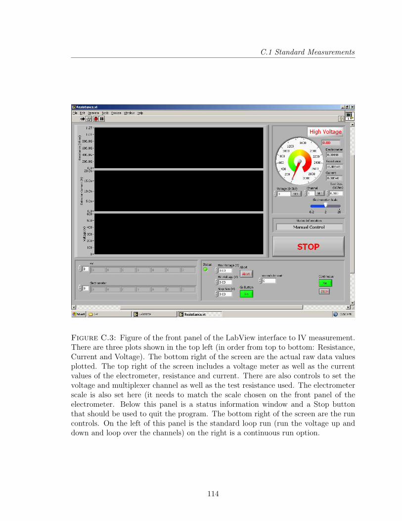
C.1 Standard Measurements
Figure C.3: Figure of the front panel of the LabView interface to IV measurement.There are three plots shown in the top left (in order from top to bottom: Resistance,Current and Voltage). The bottom right of the screen are the actual raw data valuesplotted. The top right of the screen includes a voltage meter as well as the currentvalues of the electrometer, resistance and current. There are also controls to set thevoltage and multiplexer channel as well as the test resistance used. The electrometerscale is also set here (it needs to match the scale chosen on the front panel of theelectrometer. Below this panel is a status information window and a Stop buttonthat should be used to quit the program. The bottom right of the screen are the runcontrols. On the left of this panel is the standard loop run (run the voltage up anddown and loop over the channels) on the right is a continuous run option.
114

C.1 Standard Measurements
Set
stop500
Go Button
2000
Measurement Done Status Information
Status
True
Step Size (V)
Min Voltage (V)
Max Voltage (V)
2.00
Electrometer
HV
2
%5.5f
2
2
0
1
Setting Channel
2000
Status Information
Channel
1 [0..2]
000
%5.5f
4
Test Res. (GOhm)
1000000000
Set 2
Continuous
1
0
0.00
1
0.00
Warning Light
1
1
1
0
1Y
0600.00
1000
8
High Voltage
Waiting for HV Status Information
0 [0..2]
Status InformationCurrent Error
2000Blinking
Status InformationStatus
False
Figure C.4: Figure of the full LabView block diagram for controlling the automatedIV measurements showing the overall logic of the program. The DAQ is setup on thebottom left by setting the digital and analog output ports. Following this, the mainloop is initialized which is continued until the user hits the stop button on the mainuser screen (the logic for this is on the bottom right of this figure). Within thisoverall loop, there is a state machine which is chosen by the boolean array on themiddle left of the image. This state machine specifies the task to be run and in thisimage is set up to run task ’4’ (see the number at the top of the screen) which is themain multiplexing measurement. Within this specific state there is an overall loopthat continues until the measurement completes and within this there is a sequencestructure (the ’film’ like frame) that handles the data acquisition. See Figure C.6 fora description of this data acquisition sequence. For a description of all of the statessee Figure C.5.
115
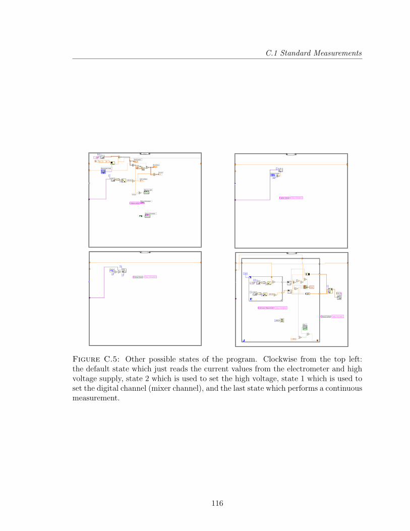
C.1 Standard Measurements
600.000
Y
1
Resistance
High Voltage
Electrometer
50.00Blinking
Warning Light
Status InformationManual Control
Current
Blinking
Status Information
1
1
0.1 1 100
Electrometer Scale
0, Default
Status InformationWaiting for Electrometer
Electrometer
0.01
1
1
Y0
100
0
2 [0..4]
1Y
0600.00
High Voltage
1
1Electrometer
Y0
Status InformationTaking Measurement
1000
4 [0..4]
-600
1
Voltage (0-3kV)
Status InformationSetting Voltage
1
Status InformationSetting Channel
Channel
2
0
1
2
-600
1
Voltage (0-3kV)
Status InformationSetting Voltage
1
Status InformationSetting Channel
Channel
2
0
1
2
stop 2
1Y
0600.00
1
1
Y0
1000
1.00E-8
Chart
10000
Status InformationContinuous Measurement
2
%5.5f
Status InformationManual Control
8
Figure C.5: Other possible states of the program. Clockwise from the top left:the default state which just reads the current values from the electrometer and highvoltage supply, state 2 which is used to set the high voltage, state 1 which is used toset the digital channel (mixer channel), and the last state which performs a continuousmeasurement.
116
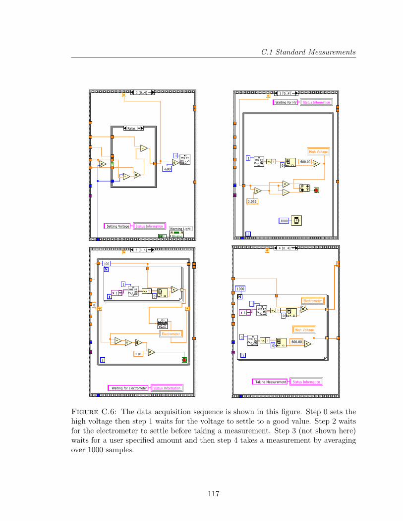
C.1 Standard MeasurementsUser Specified Wait Status Information
seconds to wait
1000
3 [0..4]
Chart
0.00
1
2.50E-8
Abort
2 [0..2]
1
-600
Blinking
Warning Light
False
Status InformationSetting Voltage
0 [0..4]
True
1Y
0600.00
High Voltage
1000
0.055
Status InformationWaiting for HV
1 [0..4]
User Specified Wait Status Information
seconds to wait
1000
3 [0..4]
Chart
0.00
1
2.50E-8
Abort
2 [0..2]
1
-600
Blinking
Warning Light
False
Status InformationSetting Voltage
0 [0..4]
True
1Y
0600.00
High Voltage
1000
0.055
Status InformationWaiting for HV
1 [0..4]
600.000
Y
1
Resistance
High Voltage
Electrometer
50.00Blinking
Warning Light
Status InformationManual Control
Current
Blinking
Status Information
1
1
0.1 1 100
Electrometer Scale
0, Default
Status InformationWaiting for Electrometer
Electrometer
0.01
1
1
Y0
100
0
2 [0..4]
1Y
0600.00
High Voltage
1
1Electrometer
Y0
Status InformationTaking Measurement
1000
4 [0..4]
Figure C.6: The data acquisition sequence is shown in this figure. Step 0 sets thehigh voltage then step 1 waits for the voltage to settle to a good value. Step 2 waitsfor the electrometer to settle before taking a measurement. Step 3 (not shown here)waits for a user specified amount and then step 4 takes a measurement by averagingover 1000 samples.
117
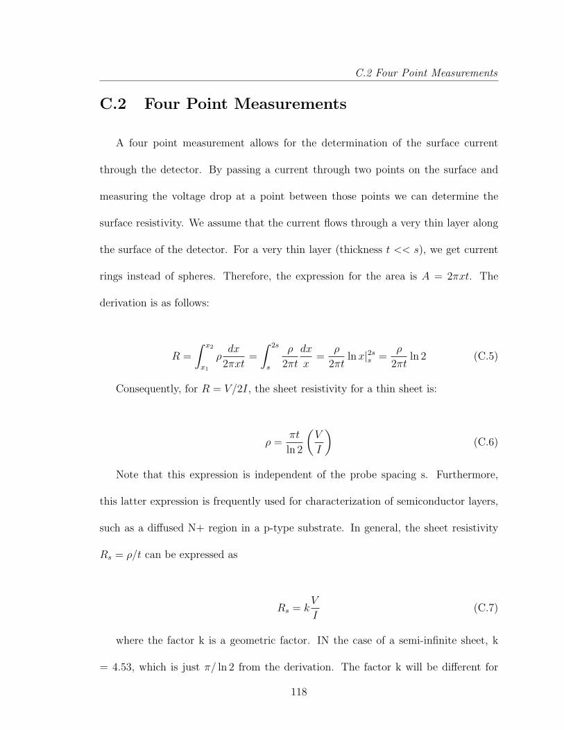
C.2 Four Point Measurements
C.2 Four Point Measurements
A four point measurement allows for the determination of the surface current
through the detector. By passing a current through two points on the surface and
measuring the voltage drop at a point between those points we can determine the
surface resistivity. We assume that the current flows through a very thin layer along
the surface of the detector. For a very thin layer (thickness t << s), we get current
rings instead of spheres. Therefore, the expression for the area is A = 2πxt. The
derivation is as follows:
R =
∫ x2
x1
ρdx
2πxt=
∫ 2s
s
ρ
2πt
dx
x=
ρ
2πtln x|2s
s =ρ
2πtln 2 (C.5)
Consequently, for R = V/2I, the sheet resistivity for a thin sheet is:
ρ =πt
ln 2
(V
I
)(C.6)
Note that this expression is independent of the probe spacing s. Furthermore,
this latter expression is frequently used for characterization of semiconductor layers,
such as a diffused N+ region in a p-type substrate. In general, the sheet resistivity
Rs = ρ/t can be expressed as
Rs = kV
I(C.7)
where the factor k is a geometric factor. IN the case of a semi-infinite sheet, k
= 4.53, which is just π/ ln 2 from the derivation. The factor k will be different for
118
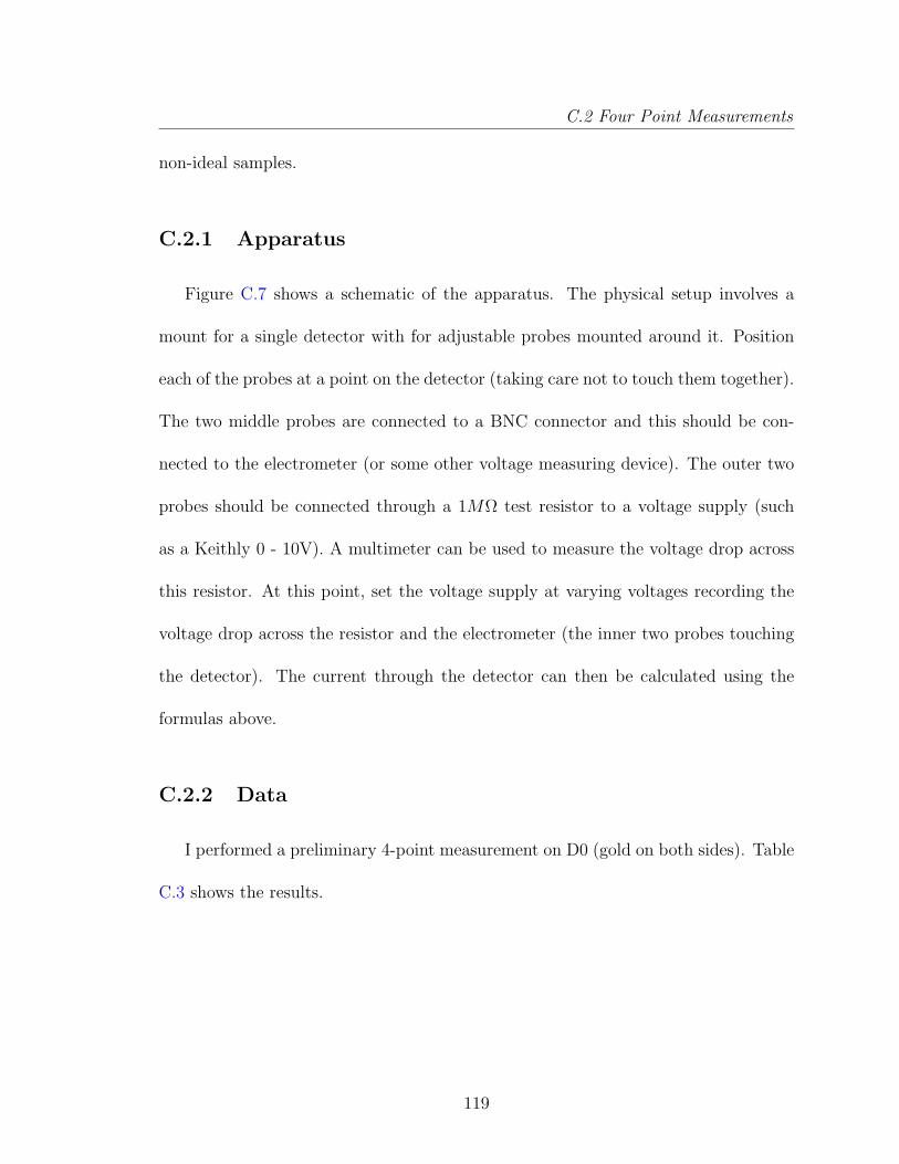
C.2 Four Point Measurements
non-ideal samples.
C.2.1 Apparatus
Figure C.7 shows a schematic of the apparatus. The physical setup involves a
mount for a single detector with for adjustable probes mounted around it. Position
each of the probes at a point on the detector (taking care not to touch them together).
The two middle probes are connected to a BNC connector and this should be con-
nected to the electrometer (or some other voltage measuring device). The outer two
probes should be connected through a 1MΩ test resistor to a voltage supply (such
as a Keithly 0 - 10V). A multimeter can be used to measure the voltage drop across
this resistor. At this point, set the voltage supply at varying voltages recording the
voltage drop across the resistor and the electrometer (the inner two probes touching
the detector). The current through the detector can then be calculated using the
formulas above.
C.2.2 Data
I performed a preliminary 4-point measurement on D0 (gold on both sides). Table
C.3 shows the results.
119

C.2 Four Point Measurements
V2
R
CZT
V3
V1 (Supply)
Figure C.7: Schematic of the
4-point measurement. V1 is the
supply voltage, R is a 1MΩ1%
resistor used in conjunction with
the V2 measurement to simulate a
current supply (shown within the
dashed box). The current is sup-
plied through the outer contacts
on the CZT and I measure the
voltage drop at V3.
Table C.3: Data for a single 4-point measurement on D0 (with gold contacts). All
values are in volts and the various measurement names are from Figure C.7.
V1 V2(±0.001) V3(±0.001) I = V2/R(nA)
0.5 0.003 0.03 3± 0.03
1.0 0.004 0.06 4± 0.04
1.5 0.006 0.09 6± 0.06
2.0 0.009 0.13 9± 0.09
2.5 0.010 0.16 10± 0.1
3.0 0.012 0.20 12± 0.2
Continued on next page.
120
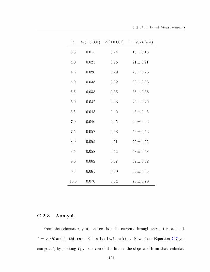
C.2 Four Point Measurements
V1 V2(±0.001) V3(±0.001) I = V2/R(nA)
3.5 0.015 0.24 15± 0.15
4.0 0.021 0.26 21± 0.21
4.5 0.026 0.29 26± 0.26
5.0 0.033 0.32 33± 0.33
5.5 0.038 0.35 38± 0.38
6.0 0.042 0.38 42± 0.42
6.5 0.045 0.42 45± 0.45
7.0 0.046 0.45 46± 0.46
7.5 0.052 0.48 52± 0.52
8.0 0.055 0.51 55± 0.55
8.5 0.058 0.54 58± 0.58
9.0 0.062 0.57 62± 0.62
9.5 0.065 0.60 65± 0.65
10.0 0.070 0.64 70± 0.70
C.2.3 Analysis
From the schematic, you can see that the current through the outer probes is
I = V2/R and in this case, R is a 1% 1MΩ resistor. Now, from Equation C.7 you
can get Rs by plotting V3 versus I and fit a line to the slope and from that, calculate
121

C.2 Four Point Measurements
Table C.4: Error Analysis (fitted line with parameters r(x) = a*x + b).
degrees of freedom (ndf) 18
rms of residuals(stdfit)=sqrt(WSSR/ndf) 0.0261646
variance of residuals(reduced chisquare)=WSSR/ndf 0.000684586
Table C.5: Results (fitted line with parameters r(x) = a*x + b).
a (Volts/nA) 0.00826403± 0.0002664(3.223%)
b (Volts) 0.0583285± 0.01069(18.33%)
the sheet resistance. Figure C.8 shows the fit and the data while the results of the
fit are given in Tables C.4 and C.5. The slope comes out to be 0.00826 V/nA which
translates to 8.26 × 10⁶Ω and if I use k = 4.53 that means that the final value I get
is Rs = 37.4MΩ which is on the order of what we expect.
122

C.2 Four Point Measurements
0
0.1
0.2
0.3
0.4
0.5
0.6
0.7
0 10 20 30 40 50 60 70 80
Vol
tage
(V
olts
)
Current (NanoAmps)
Figure C.8: The fit and the
data.
123

Appendix D
Data Acquisition System for X-ray
Spectroscopy
D.1 Apparatus
This system is setup to acquire a spectrum from a CZT detector using a fast
500Mhz oscilloscope readout for three pixels as well as the cathode so as to provide
timing information. Sixteen more pixels are read out using an ASIC and only provide
amplitude information. A schematic of the system is shown in Figure D.1 and an
image of the detector mounted as well as the pixel layout is shown in Figure D.2.
D.2 Code
#include <iostream>
#include <errno . h>
124
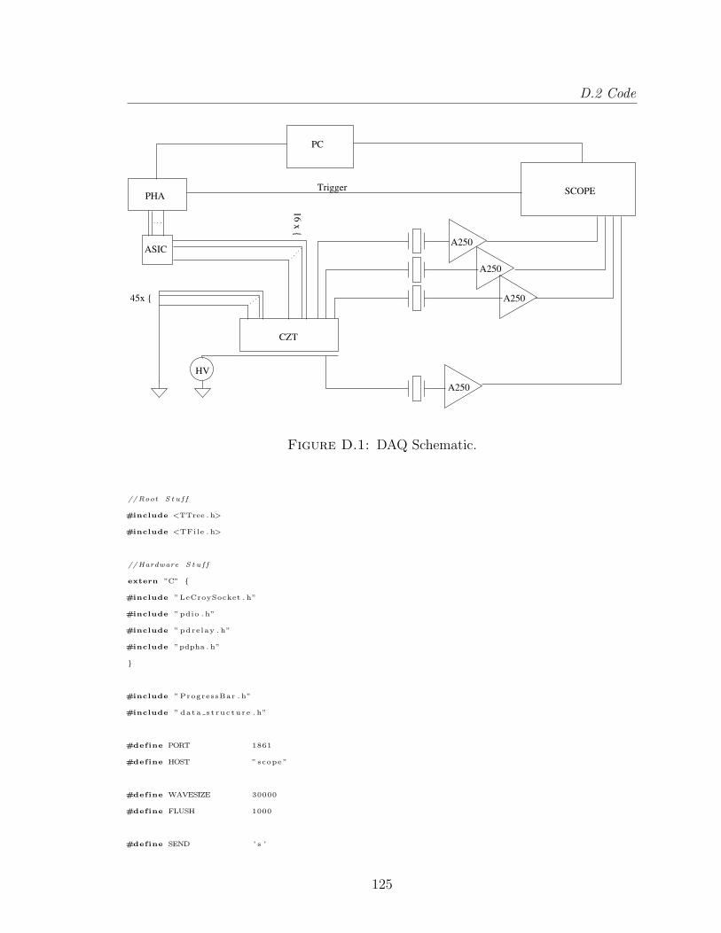
D.2 Code
A250
A250
A250
A250
CZT
PC
16 x
PHATrigger
HV
45x
SCOPE
ASIC
Figure D.1: DAQ Schematic.
//Root S t u f f
#include <TTree . h>
#include <TFile . h>
//Hardware S t u f f
extern ”C”
#include ”LeCroySocket . h”
#include ”pdio . h”
#include ” pdre lay . h”
#include ”pdpha . h”
#include ”ProgressBar . h”
#include ” da ta s t ru c tu r e . h”
#define PORT 1861
#define HOST ” scope ”
#define WAVESIZE 30000
#define FLUSH 1000
#define SEND ’ s ’
125

D.2 Code
1 2 3 4 5 6 7 8
9 10 11 12 13 14 15 16
17
33 34
18 23 24
32312625
19 20 21 22
27 28 29 30
35 36 38
41 46 47 48
49 50 51 52 54
59 60 61 62
37 39 40
45444342
53 55 56
646357 58
Figure D.2: Pixel Layout. The panel on the left shows a CZT detector mounted inthe DAQ system pointing out the location of the top left corner. Using this locationas a reference, the right panel diagrams the pixel mapping. The pixels in green areconnected to the A250 and through the oscilloscope while the pixels in yellow areconnected to the ASIC and through the PHA boards. Pixels in white are grounded.
#define READ ’ r ’
#define QUIT ’Q’
#define MENU ’m’
#define GRABPHA ’p ’
#define GRABSCP ’ g ’
#define GRABN ’n ’
#define CHANNELS ’ c ’
#define HEADER ’h ’
#define SETTHRESH ’ t ’
#define KWICK ’k ’
#define DEBUG ’d ’
using namespace std ;
stat ic int ScopeSend ( char∗ , int ) ;
stat ic void ScopeRead (void ) ;
stat ic void grabP ( int mesg , int disp , int type ) ;
stat ic void qu i t (void ) ;
stat ic void grabS ( int ) ;
stat ic void grabN ( int ) ;
stat ic void SetChannels ( ) ;
stat ic double GetTrigTime (void ) ;
126

D.2 Code
stat ic void GetHeader (void ) ;
stat ic f loat GetOption ( int , char ∗ ) ;
stat ic void WaitCoin (void ) ;
stat ic void SetThresholds ( int ) ;
stat ic void SetTr iggerScope (void ) ;
stat ic void I n i tTr e e s (TTree∗∗ , TTree∗∗ , TTree ∗∗ ) ;
stat ic void DeleteTrees (TTree∗∗ , TTree∗∗ , TTree ∗∗ ) ;
stat ic void WriteTrees ( char∗ ,TTree∗ ,TTree∗∗ , TTree∗ , TTree ∗ ) ;
stat ic void QuickSetChans ( int ) ;
stat ic void DebugSwitch ( ) ;
int sock fd ; /∗ Socke t Re ference ∗/
stat ic int Npha ;
stat ic int Nwds ;
stat ic unsigned short ∗D; /∗ data b u f f e r ∗/
stat ic short Intdac = 200 ; /∗ i n t e r n a l dac v a l u e ∗/
bool debug = fa l se ;
#define NLINES 3
char ∗progmenu [NLINES ] ;
#define LINELEN 80
stat ic void initmenu (void ) ;
stat ic void menu(void ) ;
char ∗menuformat [ ] =
”%c=send %c=grabpha %c=channe ls %c=menu ” ,
”%c=read %c=grabScp %c=grabN %c=header ” ,
”%c=setTh %c=kwick %c=debug %c=qui t ” ,
;
int waveforms [ 4 ] [WAVESIZE ] ;
I n t t pha [ 1 6 ] ;
DATA data ;
HEAD head ;
int main ( int argc , char ∗argv [ ] )
int i ;
char key ;
char bu f f e r [ 2 5 6 ] ;
127

D.2 Code
//Connect to t h e Scope
sock fd = connectToScope (PORT,HOST) ;
i f ( sock fd < 0)
cout << ”ERROR opening socket ” << endl ;
else
cout << ”Connected to scope . ” << endl ;
i f ( errno )
f p r i n t f ( s tder r , ”Can ’ t i n i t i a l i z e board (%s )\n” , s t r e r r o r ( errno ) ) ;
// I n i t i a l i z e PHA Boards
p r i n t f ( ” I n i t i a l i z i n g Board . . . \ n” ) ;
pdpha in i t ( ) ;
i f ( errno )
f p r i n t f ( s tder r , ”Can ’ t i n i t i a l i z e board (%s )\n” , s t r e r r o r ( errno ) ) ;
else
p r i n t f ( ” I n i t i a l i z e d .\n” ) ;
Npha = pdpha get nphadet ( ) ;
Nwds = 6 + (Npha ∗ 12 ) ;
D = ( short unsigned int ∗) mal loc (Nwds ∗ s izeof ( short ) ) ;
i f (D == NULL)
f p r i n t f ( s tder r , ”%s : can ’ t mal loc\n” , argv [ 0 ] ) ;
e x i t ( 1 ) ;
SetThresholds ( 1 ) ;
initmenu ( ) ;
while (1 )
cout << ” : ” ;
c in >> key ;
switch ( key )
case SEND:
ScopeSend ( bu f f e r , 1 ) ;
break ;
case READ:
ScopeRead ( ) ;
break ;
case QUIT:
128
D.2 Code
qu i t ( ) ;
break ;
case MENU:
initmenu ( ) ;
break ;
case GRABPHA:
grabP ( 1 , 1 , 0 ) ;
break ;
case GRABSCP:
grabS ( 1 ) ;
break ;
case GRABN:
grabN ( 0 ) ;
break ;
case CHANNELS:
SetChannels ( ) ;
break ;
case HEADER:
GetHeader ( ) ;
break ;
case SETTHRESH:
SetThresholds ( 0 ) ;
break ;
case KWICK:
QuickSetChans ( 0 ) ;
break ;
case DEBUG:
DebugSwitch ( ) ;
break ;
default :
i f ( key != ’\ r ’ && key != ’\n ’ )
p r i n t f ( ” %c? What i s that ?\n\ r ” , key ) ;
break ;
stat ic void SetChannels ( )
int i ;
for ( i =0; i <5; i++)
i f ( i==4)
cout << ” Disab le /Enable PHA’ s (1/0)? ” << endl ;
129
D.2 Code
else
cout << ” Disab le /Enable Channel ” << i+1 << ” (1/0)? ” << endl ;
c in >> head . channe ls [ i ] ;
for ( i =0; i <5; i++)
i f ( i==4)
cout << ” Tr igger from PHA’ s (1/0)? ” << endl ;
else
cout << ” Tr igger from Channel ” << i+1 << ” (1/0)? ” << endl ;
c in >> head . t r i g g e r s [ i ] ;
i f ( head . t r i g g e r s [ i ] )
data . t r i g g e r = i ;
stat ic void QuickSetChans ( int cho i c e )
int i ;
//A250 Se t Up
i f ( cho i c e == 0)
for ( i =0; i <4; i++)
head . channe ls [ i ] = true ;
head . channe ls [ 4 ] = fa l se ;
for ( i =1; i <4; i++)
head . t r i g g e r s [ i ] = true ;
head . t r i g g e r s [ 0 ] = fa l se ;
head . t r i g g e r s [ 4 ] = fa l se ;
cout << ”Set up channe ls f o r A250 ( Tr igge r ing on 2 , 3 , 4 ) . ” << endl ;
stat ic int ScopeSend ( char∗ buf f e r , int type )
s t r i n g s t r ;
int n ;
130
D.2 Code
i f ( type == 1)
cout << ” Please ente r the message : \ r ” << endl ;
f g e t s ( bu f f e r , 255 , s td in ) ;
f g e t s ( bu f f e r , 255 , s td in ) ;
i f ( debug )
cout << ”ScopeSend : ’ ” << bu f f e r << ” ’ ” << endl ;
n = sendToScope ( bu f f e r , sock fd ) ;
else
i f ( debug )
cout << ”ScopeSend : ’ ” << bu f f e r << ” ’ ” << endl ;
n = sendToScope ( bu f f e r , sock fd ) ;
i f (n < 0)
cout << ”ERROR wr i t ing to socket ( ’ ” << bu f f e r << ” ’ ) ” << endl ;
return n ;
stat ic void ScopeRead (void )
char bu f f e r [ 2 5 6 ] ;
int waveform [WAVESIZE ] ;
int n , i ;
bzero ( bu f f e r , 2 5 6 ) ;
n = readFromScope ( bu f f e r , sockfd , waveform ) ;
i f (n < 0)
cout << ”ERROR reading from socket ” << endl ;
p r i n t f ( ”%s\n” , bu f f e r ) ;
i f (n > 256)
cout << ”Recieved Waveform of s i z e ” << n << endl ;
stat ic void grabS ( int type )
char bu f f e r [ 2 5 6 ] ;
int n , i ;
131

D.2 Code
bool f i r s t = true ;
//Read the channe l s
for ( i =0; i <4; i++)
i f ( head . channe ls [ i ] )
i f ( type == 1 && f i r s t )
cout << ”Enter a t r i g g e r Channel” << endl ;
c in >> data . t r i g g e r ;
SetTr iggerScope ( ) ;
ScopeSend ( ”arm ; wait ” , 0 ) ;
s p r i n t f ( bu f f e r , ”c%i : wf? dat1” , i +1);
ScopeSend ( bu f f e r , 0 ) ;
bzero ( bu f f e r , 2 5 6 ) ;
n = readFromScope ( bu f f e r , sockfd ,&waveforms [ i ] [ 0 ] ) ;
i f (n < 0)
cout << ”ERROR reading from socket ” << endl ;
//Ok , don ’ t know why t h i s works , bu t i t does . Sometimes you have to
// ask aga in n i c e l y .
i f ( bu f f e r [ 1 1 ] != ’#’ )
n = readFromScope ( bu f f e r , sockfd ,&waveforms [ i ] [ 0 ] ) ;
i f ( debug )
p r i n t f ( ”%s\n” , bu f f e r ) ;
i f (n > 256)
cout << ”Recieved Waveform of s i z e ” << n << endl ;
f i r s t = fa l se ;
stat ic void grabN ( int number )
int i , j , k ;
char f i l ename [ 2 5 6 ] ;
char temp [ 2 5 6 ] ;
cout << ”Enter a f i l e root ( eg : t e s t ) : ” << endl ;
c in >> f i l ename ;
// c r e a t e t h e t r e e s
TTree ∗wave [ 4 ] ;
132

D.2 Code
TTree ∗pha T ;
TTree ∗ event ;
TTree ∗header = new TTree ( ”header ” , ”Run Informat ion ” ) ;
ProgressBar ∗ prog r e s s ;
// s e t up t he TTrees
header−>Branch ( ”head” , &head , ” v e r t i c a l g a i n [ 4 ] /F : v e r t i c a l o f f s e t [ 4 ] /F : h o r i z i n t e r v a l [ 4 ] /F : h o r i z o f f s e t [ 4 ] /F : p o i n t s p e r s c r e e n [ 4 ] / I : t r i g g e r s [ 5 ] / I : cathode / I : channe ls [ 5 ] / I ” ) ;
I n i tTr e e s (wave ,&pha T ,&event ) ;
// s e t up t he l o o p i n g
i f (number<1)
cout << ”Enter the number o f events (0 to e x i t ) : ” << endl ;
c in >> number ;
// ProgressBar p r o g r e s s ( number , ” Chan 0” ) ;
cout << ”Enter in the Cathode Channel . ” << endl ;
c in >> head . cathode ;
// F i l l t h e header
GetHeader ( ) ;
header−>F i l l ( ) ;
//Grab t he data and f i l l t h e waveforms
k=0;
for ( data . t r i g g e r =0; data . t r i g g e r <5; data . t r i g g e r++)
i f ( head . t r i g g e r s [ data . t r i g g e r ] )
s p r i n t f ( temp , ”Chan %i ” , data . t r i g g e r +1);
i f ( ! debug )
p rog r e s s = new ProgressBar (number , temp ) ;
SetTr iggerScope ( ) ;
for ( i =0; i<number ; i++)
data . eventnum = i+k ;
WaitCoin ( ) ;
grabS ( 0 ) ;
i f ( head . channe ls [ 4 ] )
grabP ( 1 , 0 , 1 ) ;
pha T−>F i l l ( ) ;
for ( j =0; j <4; j++)
i f ( head . channe ls [ j ] )
i f ( debug )
cout << ” F i l l i n g Waveform ” << j << endl ;
133
D.2 Code
wave [ j ]−> F i l l ( ) ;
data . time = GetTrigTime ( ) ;
event−>F i l l ( ) ;
// Save to d i s c eve r so o f t e n f o r s a f e t y !
i f ( data . eventnum%FLUSH == 0 && data . eventnum > 0)
WriteTrees ( f i l ename , header , wave , pha T , event ) ;
De leteTrees (wave ,&pha T ,&event ) ;
I n i tTr e e s (wave ,&pha T ,&event ) ;
i f ( ! debug )
progress−>pr in t ( i ) ;
i f ( debug )
cout << ”Event ” << i+k << endl ;
k+=number ;
i f ( ! debug )
progress−>pr in tC l ea r ( ) ;
delete prog r e s s ;
cout << ”Fin i shed with channel ” << data . t r i g g e r+1 << ” ( ” << i << ” events ) . ” << endl ;
WriteTrees ( f i l ename , header , wave , pha T , event ) ;
De leteTrees (wave ,&pha T ,&event ) ;
stat ic void
grabP ( int mesg , int disp , int type )
stat ic long evtno = 0L ;
int i , j ;
unsigned long ∗ lp ;
int r e t ;
unsigned short ∗ sp ;
i f ( type==0)
data . t r i g g e r = 4 ;
SetTr iggerScope ( ) ;
134

D.2 Code
i f (mesg )
p r i n t f (
” Waiting f o r co inc idence . Press any key to stop wait .\n\ r ” ) ;
WaitCoin ( ) ;
i f ( d i sp )
p r i n t f ( ” \n\ rEvtno : %ld \n\ r ” , evtno ) ;
sp = D;
∗ sp++ = 0x90AF ; /∗ e v t s i g n a t u r e ∗/
∗ sp++ = Npha ; /∗ no . o f pha boards ∗/
lp = (unsigned long ∗) sp ;
∗ lp++ = evtno++; /∗ e v t number ∗/
∗ lp++ = c lock ( ) ; /∗ t i c k count ∗/
sp = (unsigned short ∗) lp ;
for ( i =0; i<Npha ; i++)
i f ( i == 14)
p r i n t f ( ” PRESS ANY KEY TO CONTINUE” ) ;
//GETKEY;
p r i n t f ( ” \n\ r ” ) ;
i f ( pdpha rd pha bd ( i , sp ) == (unsigned short ∗)0)
p r i n t f ( ” grab1 : pdpha rd pha bd ( ) e r r o r (%d)\n” , i ) ;
return ;
i f ( d i sp )
p r i n t f (
”%04u %04u %04u %04u %04u %04u %04u %04u ” ,
sp [ 0 ] , sp [ 1 ] , sp [ 2 ] , sp [ 3 ] , sp [ 4 ] , sp [ 5 ] , sp [ 6 ] , sp [ 7 ] ) ;
for ( j =0; j <8; j++)
pha [ i ∗8+ j ] = sp [ j ] ;
sp += 8 ;
135
D.2 Code
∗ sp++ = pdpha rd sum sca ler ( i ) ; /∗ S s c a l e r ∗/
∗ sp++ = pdpha r d s e l s c a l e r ( i ) ; /∗ SC s c a l e r ∗/
∗ sp++ = pdpha get s e l chan ( i ) ; /∗ SC channe l ∗/
∗ sp++ = pdpha pha addr map ( i ) ; /∗ board addre s s ∗/
i f ( d i sp )
p r i n t f ( ” CD=%05u SC=%05u chan=%01d bd=%d\n\ r ” ,
sp [−4] , sp [−3] , sp [−2] , sp [ −1 ] ) ;
pd i o c o i n c l r ( ) ;
stat ic void
initmenu (void )
int i ;
for ( i =0; i<NLINES ; i++)
i f ( ( progmenu [ i ] = ( char∗) mal loc ( s t r l e n (menuformat [ i ] + 1 ) ) ) == NULL)
f p r i n t f ( s tder r , ”Bad malloc (%s )\n” , s t r e r r o r ( errno ) ) ;
s p r i n t f ( progmenu [ 0 ] , menuformat [ 0 ] , SEND, GRABPHA, CHANNELS, MENU) ;
s p r i n t f ( progmenu [ 1 ] , menuformat [ 1 ] , READ, GRABSCP, GRABN, HEADER) ;
s p r i n t f ( progmenu [ 2 ] , menuformat [ 2 ] , SETTHRESH,KWICK,DEBUG,QUIT) ;
menu ( ) ;
stat ic void
menu(void )
int i ;
for ( i =0; i<NLINES ; i++)
p r i n t f ( ” %s\n” , progmenu [ i ] ) ;
stat ic void
qu i t (void )
char key ;
136
D.2 Code
cout << ”Are you sure you want to qu i t ? (y/N) : ” ;
c in >> key ;
i f ( key == ’y ’ )
cout << ” I ’m Qui t t t ing Now. ” << endl ;
e x i t ( 0 ) ;
else
cout << ”Not r e a l l y qu i t t i n g . ” << endl ;
return ;
double
GetTrigTime (void )
int dummywave [WAVESIZE ] ;
char bu f f e r [ 2 5 6 ] ;
s t r i n g temp , t r i g t ime ;
double h ,m, s , seconds ;
int n , t1 , t2 , i ;
bzero ( bu f f e r , 2 5 5 ) ;
i f ( data . t r i g g e r <4)
s p r i n t f ( bu f f e r , ”c%i : insp ? ’ t r i g g e r t ime ’ ” , data . t r i g g e r +1);
else
s p r i n t f ( bu f f e r , ” c1 : insp ? ’ t r i g g e r t ime ’ ” ) ;
ScopeSend ( bu f f e r , 0 ) ;
bzero ( bu f f e r , 2 5 5 ) ;
n = readFromScope ( bu f f e r , sockfd , dummywave ) ;
i f (n < 0)
cout << ”ERROR reading from socket ( ” << bu f f e r << ” ) ” << endl ;
i f ( debug )
cout << bu f f e r ;
i =0;
//Ok , don ’ t know why t h i s works , bu t i t does . Sometimes you have to
// ask aga in n i c e l y .
while ( bu f f e r [ i ] != ’T ’ && i <256)
i++;
i f ( bu f f e r [ i ] != ’T ’ )
i f ( debug )
cout << ”Asking f o r time again . ” << endl ;
137
D.2 Code
bzero ( bu f f e r , 2 5 5 ) ;
i f ( data . t r i g g e r <4)
s p r i n t f ( bu f f e r , ”c%i : insp ? ’ t r i g g e r t ime ’ ” , data . t r i g g e r +1);
else
s p r i n t f ( bu f f e r , ” c1 : insp ? ’ t r i g g e r t ime ’ ” ) ;
ScopeSend ( bu f f e r , 0 ) ;
bzero ( bu f f e r , 2 5 5 ) ;
n = readFromScope ( bu f f e r , sockfd , dummywave ) ;
temp = &bu f f e r [ 8 ] ;
t1 = temp . f i n d f i r s t o f ( ”=” , 0 ) ;
t1 = temp . f i n d f i r s t o f ( ”=” , t1 +1);
t2 = temp . f i n d f i r s t o f ( ”\”” , t1 ) ;
t r i g t ime = temp . subs t r ( t1+2, t2−t1 −2);
h = ato f ( t r i g t ime . subs t r ( 0 , 2 ) . c s t r ( ) ) ;
m = ato f ( t r i g t ime . subs t r ( 3 , 2 ) . c s t r ( ) ) ;
s = ato f ( t r i g t ime . subs t r ( 6 , 1 0 ) . c s t r ( ) ) ;
seconds = s+60∗m+60∗60∗h ;
i f ( debug )
cout << ”Trig Time : ”<< h <<” : ”<< m <<” : ”<< s << ” ( ”<< seconds <<” s t o t a l ) ” << endl ;
return seconds ;
void
GetHeader (void )
int i ;
for ( i =0; i <4; i++)
head . p o i n t s p e r s c r e e n [ i ] = ( int ) GetOption ( i +1,”PNTS PER SCREEN” ) ;
head . v e r t i c a l g a i n [ i ] = GetOption ( i +1,”VERTICAL GAIN” ) ;
head . v e r t i c a l o f f s e t [ i ] = GetOption ( i +1,” v e r t i c a l o f f s e t ” ) ;
head . h o r i z i n t e r v a l [ i ] = GetOption ( i +1,” h o r i z i n t e r v a l ” ) ;
head . h o r i z o f f s e t [ i ] = GetOption ( i +1,” h o r i z o f f s e t ” ) ;
138

D.2 Code
f loat
GetOption ( int channel , char∗ opt ion )
int dummywave [WAVESIZE ] ;
char bu f f e r [ 2 5 6 ] ;
f loat value ;
int n ;
bzero ( bu f f e r , 2 5 5 ) ;
s p r i n t f ( bu f f e r , ”c%i : insp ? ’%s ’ ” , channel , opt ion ) ;
ScopeSend ( bu f f e r , 0 ) ;
bzero ( bu f f e r , 2 5 5 ) ;
n = readFromScope ( bu f f e r , sockfd , dummywave ) ;
va lue = ato f (&bu f f e r [ 3 0 ] ) ;
i f ( debug )
cout << bu f f e r ;
cout << value << endl ;
return value ;
void
SetThresholds ( int i n i t )
int i ;
i f ( ! i n i t )
cout << ”Enter a thre sho ld value . ” << endl ;
c in >> Intdac ;
p r i n t f ( ” Se t t ing th r e sho ld s . . . \ n” ) ;
for ( i =0; i < Npha ; i++)
pdpha se t thr dac ( i , Intdac ) ;
p r i n t f ( ”Thresholds s e t .\n” ) ;
void
WaitCoin (void )
139
D.2 Code
int i =0;
int sum=0;
i f ( head . channe ls [ 4 ] )
i f ( debug )
p r i n t f ( ” Clear ing PHA co inc idnece .\n” ) ;
pd i o c o i n c l r ( ) ;
i f ( debug )
p r i n t f ( ” . . Cleared .\n” ) ;
for ( i =0; i <4; i++)
sum+=head . channe ls [ i ] ;
i f (sum>0)
ScopeSend ( ”arm” , 0 ) ;
//You need to wa i t a b i t a f t e r s end ing t h e arm command to t h e scope
// Otherwise , t h e pd co in might g e t t h e r e b e f o r e t h e scope i s ready
us l e ep (500000) ;
i f ( debug )
p r i n t f ( ”PHA Waiting . . . \ n” ) ;
while ( ! pd i o co in c i d enc e ( ) )
// i f ( k b h i t ( ) )
// g e t c h ( ) ;
// p r i n t f (” Cance l l e d \n\ r ” ) ;
// r e t u rn ;
//
else
ScopeSend ( ”arm ; wait ” , 0 ) ;
void
SetTr iggerScope (void )
140

D.2 Code
char bu f f e r [ 2 5 6 ] ;
int n ;
// Stop t he scope This cou l d p r o b a b l y be done e l s ewh e r e to make
// the a q u i s i t i o n f a s t e r .
ScopeSend ( ” stop ” , 0 ) ;
// Se t t h e t r i g g e r This cou l d p r o b a b l y be done e l s ewh e r e to make
// the a q u i s i t i o n f a s t e r .
// Se t up th e scope to t r i g g e r e x t e r n a l l y i f we ’ re t r i g g e r i n g o f f
// o f t h e PHA’ s
bzero ( bu f f e r , 2 5 6 ) ;
i f ( data . t r i g g e r <4)
s p r i n t f ( bu f f e r , ” t r s e edge , sr , c%i ” , data . t r i g g e r +1);
else
s p r i n t f ( bu f f e r , ” t r s e edge , sr , ex” ) ;
ScopeSend ( bu f f e r , 0 ) ;
void
I n i tTr e e s (TTree ∗∗wave , TTree ∗∗pha T , TTree ∗∗ event )
// This f u n c t i o n i n i t i a l i z e s t h e t r e e s f o r data a c q u i s i t i o n .
int i ;
char temp1 [ 5 0 ] , temp2 [ 5 0 ] ;
i f ( debug )
cout << ” I n i t i a l l i z i n g event Tree . ” << endl ;
∗ event = new TTree ( ”data” , ”Event Informat ion ” ) ;
(∗ event)−>Branch ( ”data” ,&data , ”eventnum/ I : time/D: t r i g g e r / I ” ) ;
for ( i =0; i <4; i++)
i f ( head . channe ls [ i ] )
i f ( debug )
cout << ” I n i t i a l l i z i n g wave Tree number : ” << i << endl ;
s p r i n t f ( temp1 , ”chan%i ” , i +1);
wave [ i ] = new TTree ( temp1 , temp1 ) ;
s p r i n t f ( temp2 , ”waveform[% i ] / I ” ,WAVESIZE) ;
wave [ i ]−>Branch ( temp1 ,&waveforms [ i ] [ 0 ] , temp2 ) ;
141

D.2 Code
i f ( head . channe ls [ 4 ] )
i f ( debug )
cout << ” I n i t i a l l i z i n g pha Tree . ” << endl ;
∗pha T = new TTree ( ”pha” , ”PHA Events” ) ;
(∗pha T)−>Branch ( ”pha” ,pha , ”pha [ 1 6 ] / I ” ) ;
void
DeleteTrees (TTree ∗∗wave , TTree ∗∗pha T , TTree ∗∗ event )
// This f u n c t i o n d e l e t e s t h e t r e e s f o r data a c q u i s i t i o n .
int i ;
delete (∗ event ) ;
for ( i =0; i <4; i++)
i f ( head . channe ls [ i ] )
wave [ i ]−>Delete ( ) ;
i f ( head . channe ls [ 4 ] )
delete (∗pha T ) ;
void
WriteTrees ( char ∗ f i l ename , TTree ∗header , TTree ∗∗wave , TTree ∗pha T , TTree ∗ event )
// This f u n c t i o n w r i t e s t h e data to f i l e
int j ;
char o u t f i l e [ 2 5 6 ] ;
s p r i n t f ( o u t f i l e , ”%s−%i . root ” , f i l ename , data . eventnum ) ;
i f ( debug )
cout << ”Flushing data to d i s c . ” << endl ;
cout << ”Filename : ” << o u t f i l e << endl ;
142
D.2 Code
TFile ∗ f = new TFile ( o u t f i l e , ”RECREATE” ) ;
i f ( debug )
cout << ”Writing t r e e s . . . ” << endl ;
// f−>Flush ( ) ;
header−>Write ( ) ;
i f ( head . channe ls [ 4 ] )
pha T−>Write ( ) ;
event−>Write ( ) ;
for ( j =0; j <4; j++)
i f ( head . channe ls [ j ] )
wave [ j ]−>Write ( ) ;
i f ( debug )
cout << ”Done . ” << endl ;
cout << ”Clos ing f i l e . . . ”<<endl ;
f−>Write ( ) ;
f−>Close ( ) ;
i f ( debug )
cout << ”Done . ” << endl ;
delete f ;
void
DebugSwitch ()
debug = ! debug ;
cout << ”Debug i s now ” << debug << endl ;
143
Appendix E
Upper Limit Calculation
The following code computes an upper limit based on the Baysian method of
Helene (1983). This specific algorithm was used for the upper limit calculation pre-
sented in this thesis. Note that it depends on the GNU Scientific Library (GSL) for
the gaussian statistics computations.
E.1 Code
#include <g s l / g s l c d f . h>
double upper (double , double , double ) ;
int main ( int argc , char ∗argv [ ] )
double sigma
double s i gma in pe r c en t ;
double f lux , e r r o r ;
c in >> sigma ;
c in >> f l u x ;
c in >> e r r o r ;
144
E.1 Code
// Ca l c u l a t e t h e sigma wanted in pe r c en t .
s i gma in pe r c en t = 1 − 1 .∗ g s l c d f g au s s i an Q ( sigma , 1 ) ;
//Compute t h e upper l i m i t based on the f l u x and e r r o r
cout << upper ( f lux , e r ror , s i gma in pe r c en t ) << endl ;
double upper (double mu, double er ror , double sigma )
double upper ;
double t o t a l p o s ;
double con f i d ence po s ;
//The pe r c en t a g e o f t h e gau s s i an above 0 i s computed here
//The ’Q ’ c d f i s t h e c d f from some va l u e x up to i n f . I f
// you have a gaus s i an c en t e r e d on mu, then to f i n d th e pos
// percen tage , you sum from −mu up to i n f .
t o t a l p o s = g s l c d f g au s s i an Q(−mu, e r r o r ) ;
//The pe r c en t a g e o f t h e gaus ian w i t h i n t h e c on f i d enc e i n t e r v a l
// above ze ro i s
con f i d ence po s = (1 . 0 − sigma )∗ t o t a l p o s ;
//The ’ Qinv ’ f u n c t i o n f i n d s t h e v a l u e o f x f o r a g i v en pe r c en t a g e
//We ’ re l o o k i n g f o r t h e 90% o f t h e p o s i t i v e p e r c en t a g e and upper
// then g i v e s t h e v a l u e o f t h e e x c e s s a t t h e 90% o f t h e p o s i t i v e
// pe r c en t a g e −> i e . t h e 90% con f i d enc e l i m i t .
upper = g s l c d f g au s s i an Q inv ( con f idence pos , e r r o r ) ;
//You have to add ’mu ’ to t h e upper l i m i t because t h e z e ro l e v e l
// i s d i f f e r e n t from the s tandard gaus s i an and the one we want to
// c a l c u l a t e
upper+=mu;
return upper ;
145

Bibliography
Aharonian, F., Akhperjanian, A. G., Aye, K.-M., Bazer-Bachi, A. R., Beilicke,M., Benbow, W., Berge, D., Berghaus, P., Bernlohr, K., Bolz, O., Boisson,C., Borgmeier, C., Breitling, F., Brown, A. M., Bussons Gordo, J., Chadwick,P. M., Chitnis, V. R., Chounet, L.-M., Cornils, R., Costamante, L., Degrange, B.,Djannati-Ataı, A., O’C. Drury, L., Ergin, T., Espigat, P., Feinstein, F., Fleury, P.,Fontaine, G., Funk, S., Gallant, Y., Giebels, B., Gillessen, S., Goret, P., Guy, J.,Hadjichristidis, C., Hauser, M., Heinzelmann, G., Henri, G., Hermann, G., Hinton,J. A., Hofmann, W., Holleran, M., Horns, D., de Jager, O. C., Jung, I., Khelifi, B.,Komin, N., Konopelko, A., Latham, I. J., Le Gallou, R., Lemoine, M., Lemiere,A., Leroy, N., Lohse, T., Marcowith, A., Masterson, C., McComb, T. J. L., deNaurois, M., Nolan, S. J., Noutsos, A., Orford, K. J., Osborne, J. L., Ouchrif, M.,Panter, M., Pelletier, G., Pita, S., Pohl, M., Puhlhofer, G., Punch, M., Rauben-heimer, B. C., Raue, M., Raux, J., Rayner, S. M., Redondo, I., Reimer, A., Reimer,O., Ripken, J., Rivoal, M., Rob, L., Rolland, L., Rowell, G., Sahakian, V., Sauge,L., Schlenker, S., Schlickeiser, R., Schuster, C., Schwanke, U., Siewert, M., Sol, H.,Steenkamp, R., Stegmann, C., Tavernet, J.-P., Theoret, C. G., Tluczykont, M., vander Walt, D. J., Vasileiadis, G., Vincent, P., Visser, B., Volk, H. J., and Wagner,S. J.: 2004, Astronomy and Astrophysics 425, L13
Aharonian, F., Akhperjanian, A. G., Bazer-Bachi, A. R., Beilicke, M., Benbow, W.,Berge, D., Bernlohr, K., Boisson, C., Bolz, O., Borrel, V., Braun, I., Breitling,F., Brown, A. M., Chadwick, P. M., Chounet, L.-M., Cornils, R., Costamante,L., Degrange, B., Dickinson, H. J., Djannati-Ataı, A., O’C. Drury, L., Dubus,G., Emmanoulopoulos, D., Espigat, P., Feinstein, F., Fontaine, G., Fuchs, Y.,Funk, S., Gallant, Y. A., Giebels, B., Gillessen, S., Glicenstein, J. F., Goret, P.,Hadjichristidis, C., Hauser, M., Heinzelmann, G., Henri, G., Hermann, G., Hinton,J. A., Hofmann, W., Holleran, M., Horns, D., Jacholkowska, A., de Jager, O. C.,Khelifi, B., Komin, N., Konopelko, A., Latham, I. J., Le Gallou, R., Lemiere, A.,Lemoine-Goumard, M., Leroy, N., Lohse, T., Martin, J. M., Martineau-Huynh, O.,Marcowith, A., Masterson, C., McComb, T. J. L., de Naurois, M., Nolan, S. J.,Noutsos, A., Orford, K. J., Osborne, J. L., Ouchrif, M., Panter, M., Pelletier, G.,Pita, S., Puhlhofer, G., Punch, M., Raubenheimer, B. C., Raue, M., Raux, J.,Rayner, S. M., Reimer, A., Reimer, O., Ripken, J., Rob, L., Rolland, L., Rowell,G., Sahakian, V., Sauge, L., Schlenker, S., Schlickeiser, R., Schuster, C., Schwanke,U., Siewert, M., Sol, H., Spangler, D., Steenkamp, R., Stegmann, C., Tavernet, J.-
146

Bibliography
P., Terrier, R., Theoret, C. G., Tluczykont, M., Vasileiadis, G., Venter, C., Vincent,P., Volk, H. J., and Wagner, S. J.: 2005, Resolving the Extragalactic BackgroundLight with gamma-ray spectra from distant blazars, astro-ph/0508073
Aharonian, F. A.: 2005, American Astronomical Society Meeting Abstracts 207,
Alexandreas, D. E., Berley, D., Biller, S., Dion, G. M., Goodman, J. A., Haines,T. J., Hoffman, C. M., Horch, E., Lu, X.-Q., Sinnis, C., Yodh, G. B., and Zhang,W.: 1993, Nuclear Instruments and Methods in Physics Research A 328, 570
Barret, H. H., Eskin, J. D., and Barber, H. B.: 1995, Phys. Rev. Let. 75, 156
Benbow et. al., W.: 2005, in F. A. Aharonian, H. J. Volk, and D. Horns (eds.), AIPConf. Proc. 745: High Energy Gamma-Ray Astronomy, pp 611–616
Bergstrom, L., Ullio, P., and Buckley, J. H.: 1998, Astroparticle Physics 9, 137
Blanton, E. L.: 2004, in T. Reiprich, J. Kempner, and N. Soker (eds.), The Riddle ofCooling Flows in Galaxies and Clusters of galaxies, pp 181–+
Blanton, E. L., Sarazin, C. L., McNamara, B. R., and Wise, M. W.: 2001, ApJL 558,L15
Blasi, P. and Colafrancesco, S.: 1999, Astroparticle Physics 12, 169
Boehringer, H., Voges, W., Fabian, A. C., Edge, A. C., and Neumann, D. M.: 1993,MNRAS 264, L25
Bohringer, H., Matsushita, K., Churazov, E., Ikebe, Y., and Chen, Y.: 2002, Astron-omy and Astrophysics 382, 804
Bolotnikov, A. E., Chen, C. M. H., Cook, W. R., Harrison, F. A., Kuvvetli, I., andSchindler, S. M.: 2002, IEEE Transactions on Nuclear Science 49, 1941
Bolotnikov, A. E., Cook, W. R., Harrison, F. A., Wong, A.-S., Schindler, S. M., andEichelberger, A. C.: 1999, Nuclear Instruments and Methods in Physics ResearchA 432, 326
Bowyer, S. and Berghofer, T. W.: 1998, ApJ 506, 502
Buckley, J. H., Akerlof, C. W., Carter-Lewis, D. A., Catanese, M., Cawley, M. F.,Connaughton, V., Fegan, D. J., Finley, J. P., Gaidos, J. A., Hillas, A. M., Kren-nrich, F., Lamb, R. C., Lessard, R. W., McEnery, J. E., Mohanty, G., Quinn, J.,Rodgers, A. J., Rose, H. J., Rovero, A. C., Schubnell, M. S., Sembroski, G., Srini-vasan, R., Weekes, T. C., and Zweerink, J.: 1998, Astronomy and Astrophysics329, 639
Byram, E. T., Chubb, T. A., and Friedman, H.: 1966, Science 152, 66
147

Bibliography
Carilli, C. L., Perley, R. A., and Harris, D. E.: 1994, MNRAS 270, 173
Churazov, E., Forman, W., Jones, C., and Bohringer, H.: 2003, ApJ 590, 225
Churazov, E., Sunyaev, R., Forman, W., and Bohringer, H.: 2002, MNRAS 332, 729
Clarke, T. E., Blanton, E. L., and Sarazin, C. L.: 2004, ApJ 616, 178
Colafrancesco, S.: 2001, in AIP Conf. Proc. 587: Gamma 2001: Gamma-Ray Astro-physics, p. 427
Colina, L. and Perez-Fournon, I.: 1990, ApJS 72, 41
Condon, J. J., Cotton, W. D., Greisen, E. W., Yin, Q. F., Perley, R. A., Taylor,G. B., and Broderick, J. J.: 1998, AJ 115, 1693
Conselice, C. J., Gallagher, J. S., and Wyse, R. F. G.: 2001, AJ 122, 2281
Davies, J. M. and Cotton, E. S.: 1957, Solar Energy Sci. and Eng. 1
Donahue, M. and Voit, G. M.: 2004, in J. S. Mulchaey, A. Dressler, and A. Oemler(eds.), Clusters of Galaxies: Probes of Cosmological Structure and Galaxy Evolu-tion, pp 143–+
Donahue, M. E., Voit, G. M., and Cavagnolo, K.: 2004, American AstronomicalSociety Meeting Abstracts 205
Edge, A. C. and Stewart, G. C.: 1991, MNRAS 252, 414
Edge, D. O., Shakeshaft, J. R., McAdam, W. B., Baldwin, J. E., and Archer, S.:1959, Mem. R. Astron. Soc. 68, 37
Enßlin, T. A. and Biermann, P. L.: 1998, Astronomy and Astrophysics 330, 90
Fabian, A. C.: 1994, Ann. Rev. Astron. Astrophys. 32, 277
Fabian, A. C., Hu, E. M., Cowie, L. L., and Grindlay, J.: 1981, ApJ 248, 47
Fabian, A. C., Sanders, J. S., Taylor, G. B., Allen, S. W., Crawford, C. S., Johnstone,R. M., and Iwasawa, K.: 2006, MNRAS 366, 417
Fabian, A. C., Zarneck, J. C., Culhane, J. L., Hawkins, F. J., Peacock, A., Pounds,K. A., and Parkinson, J. H.: 1974, ApJL 189, L59+
Falcone, A. D., Badran, H. M., Blaylock, G., Bond, I. H., Boyle, P. J., Bradbury,S. M., Buckley, J. H., Byrum, K., Carter-Lewis, D. A., Celik, O., Cogan, P., Cui,W., Daniel, M., de La Calle Perez, I., Dowkontt, P., Duke, C., Fegan, D. J., Fegan,S. J., Finley, J. P., Fortson, L. F., Gammell, S., Gibbs, K., Gillanders, G. H.,Grube, J., Guiterrez, K. J., Hall, J., Hanna, D., Holder, J., Horan, D., Hughes, S.,
148

Bibliography
Humensky, T. B., Jung, I., Kenny, G. E., Kertzman, M., Kieda, D., Kildea, J.,Knapp, J., Kosack, K., Krawczynski, H., Krennrich, F., Lang, M. J., Le Bohec, S.,Linton, E., Lloyd-Evans, J., Mendoza, D., Merriman, A., Milovanovic, A., Moriarty,P., Nagai, T., Olevitch, M., Ong, R. A., Pallassini, R., Perkins, J., Petry, D., Pizlo,F., Pohl, M., Power-Mooney, B., Quinn, J., Quinn, M., Ragan, K., Rebillot, P.,Reynolds, P. T., Rose, H. J., Schroedter, M., Sembroski, G. H., Swordy, S. P.,Syson, A., Valcarcel, L., Vassiliev, V. V., Wagner, R., Wakely, S. P., Walker, G.,Weekes, T. C., White, R. J., Zweerink, J., and VERITAS Collaboration: 2005,in F. A. Aharonian, H. J. Volk, and D. Horns (eds.), AIP Conf. Proc. 745: HighEnergy Gamma-Ray Astronomy, pp 633–638
Fegan, S. J., Badran, H. M., Bond, I. H., Boyle, P. J., Bradbury, S. M., Buckley,J. H., Carter-Lewis, D. A., Catanese, M., Celik, O., Cui, W., Daniel, M., D’Vali,M., de la Calle Perez, I., Duke, C., Falcone, A., Fegan, D. J., Finley, J. P., Fortson,L. F., Gaidos, J. A., Gammell, S., Gibbs, K., Gillanders, G. H., Grube, J., Hall,J., Hall, T. A., Hanna, D., Hillas, A. M., Holder, J., Horan, D., Jarvis, A., Jordan,M., Kenny, G. E., Kertzman, M., Kieda, D., Kildea, J., Knapp, J., Kosack, K.,Krawczynski, H., Krennrich, F., Lang, M. J., Le Bohec, S., Lessard, R. W., Linton,E., Lloyd-Evans, J., Milovanovic, A., McEnery, J., Moriarty, P., Mukherjee, R.,Muller, D., Nagai, T., Nolan, S., Ong, R. A., Pallassini, R., Petry, D., Power-Mooney, B., Quinn, J., Quinn, M., Ragan, K., Rebillot, P., Reynolds, P. T., Rose,H. J., Schroedter, M., Sembroski, G. H., Swordy, S. P., Syson, A., Vassiliev, V. V.,Wakely, S. P., Walker, G., Weekes, T. C., and Zweerink, J.: 2005, ApJ 624, 638
Feretti, L.: 2003, in Texas in Tuscany. XXI Symposium on Relativistic Astrophysics,pp 209–220
Feretti, L., Giovannini, G., Klein, U., Mack, K.-H., Sijbring, L. G., and Zech, G.:1998, Astronomy and Astrophysics 331, 475
Finley, J. P., Krennrich, F., Badran, H. M., Bond, I. H., Bradbury, S. M., Buckley,J. H., Carter-Lewis, D. A., Catanese, M., Cui, W., Dunlea, S., Das, D., de la CallePerez, I., Fegan, D. J., Fegan, S. J., Gaidos, J. A., Gibbs, K., Gillanders, G. H.,Hall, T. A., Hillas, A. M., Holder, J., Horan, D., Jordan, M., Kertzman, M., Kieda,D., Kildea, J., Knapp, J., Kosack, K., Lang, M. J., LeBohec, S., McKernan, B.,Moriarty, P., Muller, D., Ong, R., Pallassini, R., Petry, D., Quinn, J., Reay, N. W.,Reynolds, P. T., Rose, H. J., Sembroski, G. H., Sidwell, R., Stanton, N., Swordy,S. P., Vassiliev, V. V., Wakely, S. P., and Weekes, T. C.: 2001, in InternationalCosmic Ray Conference, p. 2827
Fusco-Femiano, R., dal Fiume, D., Feretti, L., Giovannini, G., Grandi, P., Matt, G.,Molendi, S., and Santangelo, A.: 1999, ApJL 513, L21
Fusco-Femiano, R., Orlandini, M., Brunetti, G., Feretti, L., Giovannini, G., Grandi,P., and Setti, G.: 2004, ApJL 602, L73
149
Bibliography
Garmire, G. P., Bautz, M. W., Ford, P. G., Nousek, J. A., and Ricker, G. R.: 2003,in X-Ray and Gamma-Ray Telescopes and Instruments for Astronomy. Edited byJoachim E. Truemper, Harvey D. Tananbaum. Proceedings of the SPIE, Volume4851, pp. 28-44 (2003)., pp 28–44
Giovannini, G. and Feretti, L.: 2000, New Astronomy 5, 335
Giovannini, G., Feretti, L., Venturi, T., Kim, K.-T., and Kronberg, P. P.: 1993, ApJ406, 399
Giovannini, G., Tordi, M., and Feretti, L.: 1999, New Astronomy 4, 141
Girardi, M., Giuricin, G., Mardirossian, F., Mezzetti, M., and Boschin, W.: 1998,ApJ 505, 74
Grindlay, J. E.: 2005, New Astronomy Review 49, 436
Gruber, D. and Rephaeli, Y.: 2002, ApJ 565, 877
Gutierrez, K. and Krawczynski, H.: 2005, ApJ 619, 161
Harris, D. E., Krawczynski, H., and Taylor, G. B.: 2002, ApJ 578, 60
Harrison et. al., F.: 2004, AAS/High Energy Astrophysics Division 8,
He, Z., Li, W., Knoll, G. F., Wehe, D. K., Berry, J., and Stahle, C. M.: 1999, NuclearInstruments and Methods in Physics Research A 422, 173
Heinz, S., Choi, Y.-Y., Reynolds, C. S., and Begelman, M. C.: 2002, ApJL 569, L79
Helene, O.: 1983, Nuclear Instruments and Methods in Physics Research 212, 319
Hillas, A. M.: 1985, in International Cosmic Ray Conference, pp 445–448
Hong, J., Bellm, E. C., Grindlay, J. E., and Narita, T.: 2004, in X-Ray and Gamma-Ray Instrumentation for Astronomy XIII. Edited by Flanagan, Kathryn A.; Sieg-mund, Oswald H. W. Proceedings of the SPIE, Volume 5165, pp. 54-62 (2004)., pp54–62
Horns, D.: 2005, Physics Letters B 607, 225
Hornschemeier, A. E., White, N. E., and Tananbaum, H.: 2005, in R. Smith (ed.), AIPConf. Proc. 774: X-ray Diagnostics of Astrophysical Plasmas: Theory, Experiment,and Observation, pp 383–389
Jackson, J. D.: 1999, Classical Electrodynamics, John Wiley and Sons, Inc, NewYork, 3rd edition
150
Bibliography
Jansen, F., Lumb, D., Altieri, B., Clavel, J., Ehle, M., Erd, C., Gabriel, C., Guainazzi,M., Gondoin, P., Much, R., Munoz, R., Santos, M., Schartel, N., Texier, D., andVacanti, G.: 2001, Astronomy and Astrophysics 365, L1
Jelley, J. V.: 1958, Cerenkov Radiation and its Applications, Pergamon Press, NewYork, NY
Jones, C. and Forman, W.: 1984, ApJ 276, 38
Jung, I., Groza, M., Perkins, J., Krawczynski, H., and Burger, A.: 2005, in R. B.James, L. A. Franks, and A. Burger (eds.), Advances in Metrology for X-Ray andEUV Optics. Edited by Assoufid, Lahsen; Takacs, Peter Z.; Taylor, John S. Pro-ceedings of the SPIE, Volume 5922, pp. 1-8 (2005)., pp 1–8
Kalemci, E. and Matteson, J. L.: 2002, Nuclear Instruments and Methods in PhysicsResearch A 478, 527
Kang, H. and Jones, T. W.: 2005, ApJ 620, 44
Kawasaki, W. and Totani, T.: 2002, ApJ 576, 679
Kempner, J. C. and Sarazin, C. L.: 2001, ApJ 548, 639
King, I. R.: 1972, ApJL 174, L123
Kneiske, T. M., Mannheim, K., and Hartmann, D. H.: 2002, Astronomy and Astro-physics 386, 1
Kosack, K.: 2005, Ph.D. thesis, Washington University in St. Louis
Kosack, K., Badran, H. M., Bond, I. H., Boyle, P. J., Bradbury, S. M., Buckley, J. H.,Carter-Lewis, D. A., Celik, O., Connaughton, V., Cui, W., Daniel, M., D’Vali, M.,de la Calle Perez, I., Duke, C., Falcone, A., Fegan, D. J., Fegan, S. J., Finley, J. P.,Fortson, L. F., Gaidos, J. A., Gammell, S., Gibbs, K., Gillanders, G. H., Grube,J., Gutierrez, K., Hall, J., Hall, T. A., Hanna, D., Hillas, A. M., Holder, J., Horan,D., Jarvis, A., Jordan, M., Kenny, G. E., Kertzman, M., Kieda, D., Kildea, J.,Knapp, J., Krawczynski, H., Krennrich, F., Lang, M. J., Le Bohec, S., Linton, E.,Lloyd-Evans, J., Milovanovic, A., McEnery, J., Moriarty, P., Muller, D., Nagai,T., Nolan, S., Ong, R. A., Pallassini, R., Petry, D., Power-Mooney, B., Quinn, J.,Quinn, M., Ragan, K., Rebillot, P., Reynolds, P. T., Rose, H. J., Schroedter, M.,Sembroski, G. H., Swordy, S. P., Syson, A., Vassiliev, V. V., Wakely, S. P., Walker,G., Weekes, T. C., and Zweerink, J.: 2004, ApJL 608, L97
Krawczynski, H.: 2002, ApJL 569, L27
Krawczynski, H., Harris, D. E., Grossman, R., Lane, W., Kassim, N., and Willis,A. G.: 2003, MNRAS 345, 1255
151

Bibliography
Leahy, D. A. and Yin, D.: 2000, MNRAS 313, 617
Li, T.-P. and Ma, Y.-Q.: 1983, ApJ 272, 317
Li, W., He, Z., Knoll, G. F., Wehe, D. K., and Berry, J. E.: 2001, Nuclear Instrumentsand Methods in Physics Research A 458, 518
Lieu, R., Ip, W.-H., Axford, W. I., and Bonamente, M.: 1999, ApJL 510, L25
Lieu, R., Mittaz, J. P. D., Bowyer, S., Breen, J. O., Lockman, F. J., Murphy, E. M.,and Hwang, C.-Y.: 1996, Science 274, 1335
Longair, M. S.: 1992, High Energy Astrophysics, Vol. 1, Cambridge University Press,Cambridge, 2nd edition
Malkan, M. A. and Stecker, F. W.: 2001, ApJ 555, 641
Mannheim, K., Hartmann, D., and Funk, B.: 1996, ApJ 467, 532
Markevitch, M., Forman, W. R., Sarazin, C. L., and Vikhlinin, A.: 1998, ApJ 503,77
Mason, K. O., Breeveld, A., Much, R., Carter, M., Cordova, F. A., Cropper, M. S.,Fordham, J., Huckle, H., Ho, C., Kawakami, H., Kennea, J., Kennedy, T., Mittaz,J., Pandel, D., Priedhorsky, W. C., Sasseen, T., Shirey, R., Smith, P., and Vreux,J.-M.: 2001, Astronomy and Astrophysics 365, L36
Matteson, J. L., Pelling, M. R., and Skelton, R. T.: 2003, in Proc. SPIE Vol. 4784,p. 1-13, X-Ray and Gamma-Ray Detectors and Applications IV, Ralph B. James;Larry A. Franks; Arnold Burger; Edwin M. Westbrook; Roger D. Durst; Eds., pp1–13
McNamara, B. R., Nulsen, P. E. J., Wise, M. W., Rafferty, D. A., Carilli, C., Sarazin,C. L., and Blanton, E. L.: 2005, Nature 433, 45
McNamara, B. R. and O’Connell, R. W.: 1989, AJ 98, 2018
McNamara, B. R., Wise, M., Nulsen, P. E. J., David, L. P., Sarazin, C. L., Bautz,M., Markevitch, M., Vikhlinin, A., Forman, W. R., Jones, C., and Harris, D. E.:2000, ApJL 534, L135
McNamara, B. R., Wise, M. W., Nulsen, P. E. J., David, L. P., Carilli, C. L., Sarazin,C. L., O’Dea, C. P., Houck, J., Donahue, M., Baum, S., Voit, M., O’Connell, R. W.,and Koekemoer, A.: 2001, ApJL 562, L149
Miley, G. K. and Perola, G. C.: 1975, Astronomy and Astrophysics 45, 223
Mitchell, R. J., Culhane, J. L., Davison, P. J. N., and Ives, J. C.: 1976, MNRAS175, 29P
152
Bibliography
Mushotzky, R. F. and Smith, B. W.: 1980, Highlights of Astronomy 5, 735
Narita, T., Bloser, P. F., Grindlay, J. E., and Jenkins, J. A.: 2000, in Proc. SPIEVol. 4141, p. 89-96, Hard X-Ray, Gamma-Ray, and Neutron Detector Physics II,Ralph B. James; Richard C. Schirato; Eds., pp 89–96
Narita, T., Bloser, P. F., Grindlay, J. E., Jenkins, J. A., and Yao, H. W.: 1999, inProc. SPIE Vol. 3768, p. 55-65, Hard X-Ray, Gamma-Ray, and Neutron DetectorPhysics, Ralph B. James; Richard C. Schirato; Eds., pp 55–65
Nevalainen, J., Oosterbroek, T., Bonamente, M., and Colafrancesco, S.: 2004, ApJ608, 166
Pacholczyk, A. G.: 1970, Radio astrophysics. Nonthermal processes in galactic andextragalactic sources, Series of Books in Astronomy and Astrophysics, San Fran-cisco: Freeman, 1970
Pedlar, A., Ghataure, H. S., Davies, R. D., Harrison, B. A., Perley, R., Crane, P. C.,and Unger, S. W.: 1990, MNRAS 246, 477
Perkins, J.-S., Badran, H. M., Blaylock, G., Bradbury, S. M., Cogan, P., Chow, Y.C. K., Cui, W., Daniel, M. K., Falcone, A. D., Fegan, S. J., Finley, J. P., Fortin, P.,Fortson, L. F., Gillanders, G. H., Gutierrez, K. J., Grube, J., Hall, J., Hanna, D.,Holder, J., Horan, D., Hughes, S. B., Kenny, G. E., Kertzman, M., Kieda, D. B.,Kildea, J., Kosack, K., Krawczynski, H., Krennrich, F., Lang, M. J., LeBohec,S., Maier, G., Moriarty, P., Ong, R. A., Pohl, M., Ragan, K., Rebillot, P. F.,Sembroski, G. H., Steele, D., Swordy, S. P., Valcarcel, L., Vassiliev, V. V., Wakely,S. P., Weekes, T. C., and Williams, D. A.: 2006, ApJ, astro-ph/0602258
Peterson, J. R., Kahn, S. M., Paerels, F. B. S., Kaastra, J. S., Tamura, T., Bleeker,J. A. M., Ferrigno, C., and Jernigan, J. G.: 2004, in T. Reiprich, J. Kempner, andN. Soker (eds.), The Riddle of Cooling Flows in Galaxies and Clusters of galaxies,pp 119–+
Pfrommer, C. and Enßlin, T. A.: 2004, Astronomy and Astrophysics 413, 17
Pigot, C., Belsole, E., Bennie, P. J., Ferrando, P., Sauvageot, J. L., Marty, P. B.,and Sembay, S.: 1999, in Proc. SPIE Vol. 3765, p. 251-264, EUV, X-Ray, andGamma-Ray Instrumentation for Astronomy X, Oswald H. Siegmund; Kathryn A.Flanagan; Eds., pp 251–264
Primack, J. R., Bullock, J. S., and Somerville, R. S.: 2005, in F. A. Aharonian,H. J. Volk, and D. Horns (eds.), AIP Conf. Proc. 745: High Energy Gamma-RayAstronomy, pp 23–33
Punch, M. and Fegan, D. J.: 1991, in AIP Conf. Proc. 220: High Energy GammaRay Astronomy, pp 321–328
153
Bibliography
Read, A. M. and Ponman, T. J.: 2003, Astronomy and Astrophysics 409, 395
Reimer, O., Pohl, M., Sreekumar, P., and Mattox, J. R.: 2003, ApJ 588, 155
Rephaeli, Y.: 1977, ApJ 218, 323
Rephaeli, Y., Gruber, D., and Blanco, P.: 1999, ApJL 511, L21
Reynolds, P. T., Akerlof, C. W., Cawley, M. F., Chantell, M., Fegan, D. J., Hillas,A. M., Lamb, R. C., Lang, M. J., Lawrence, M. A., Lewis, D. A., Macomb, D.,Meyer, D. I., Mohanty, G., O’Flaherty, K. S., Punch, M., Schubnell, M. S., Vacanti,G., Weekes, T. C., and Whitaker, T.: 1993, ApJ 404, 206
Ritz, S., Grindlay, J., Meegan, C., Michelson, P. F., and GLAST Mission Team: 2005,American Astronomical Society Meeting Abstracts 207,
Romney, J. D., Walker, R. C., Kellermann, K. I., Vermeulen, R. C., and Dhawan,V.: 1996, in IAU Symp. 175: Extragalactic Radio Sources, pp 27–+
Rosati, P., Tozzi, P., Ettori, S., Mainieri, V., Demarco, R., Stanford, S. A., Lidman,C., Nonino, M., Borgani, S., Della Ceca, R., Eisenhardt, P., Holden, B. P., andNorman, C.: 2004, AJ 127, 230
Ryu, D., Kang, H., Hallman, E., and Jones, T. W.: 2003, ApJ 593, 599
Sanders, J. S., Fabian, A. C., and Dunn, R. J. H.: 2005, MNRAS 360, 133
Sarazin, C.: 1988, X-Ray Emission from Clusters of Galaxies, Cambridge UniversityPress, Cambridge
Sarazin, C. L., O’Connell, R. W., and McNamara, B. R.: 1992, ApJL 389, L59
Scharf, C. A. and Mukherjee, R.: 2002, ApJ 580, 154
Seyfert, C. K.: 1943, ApJ 97, 28
Shakeshaft, J. R., Ryle, M., Baldwin, J. E., Elsmore, B., and Thomson, J. H.: 1955,Mem. R. Astron. Soc. 67, 106
Struble, M. F. and Rood, H. J.: 1999, ApJS 125, 35
Struder, L., Briel, U., Dennerl, K., Hartmann, R., Kendziorra, E., Meidinger, N.,Pfeffermann, E., Reppin, C., Aschenbach, B., Bornemann, W., Brauninger, H.,Burkert, W., Elender, M., Freyberg, M., Haberl, F., Hartner, G., Heuschmann, F.,Hippmann, H., Kastelic, E., Kemmer, S., Kettenring, G., Kink, W., Krause, N.,Muller, S., Oppitz, A., Pietsch, W., Popp, M., Predehl, P., Read, A., Stephan,K. H., Stotter, D., Trumper, J., Holl, P., Kemmer, J., Soltau, H., Stotter, R.,Weber, U., Weichert, U., von Zanthier, C., Carathanassis, D., Lutz, G., Richter,
154
Bibliography
R. H., Solc, P., Bottcher, H., Kuster, M., Staubert, R., Abbey, A., Holland, A.,Turner, M., Balasini, M., Bignami, G. F., La Palombara, N., Villa, G., Buttler, W.,Gianini, F., Laine, R., Lumb, D., and Dhez, P.: 2001, Astronomy and Astrophysics365, L18
Taylor, G. B., Barton, E. J., and Ge, J.: 1994, AJ 107, 1942
Taylor, G. B., Govoni, F., Allen, S. W., and Fabian, A. C.: 2001, MNRAS 326, 2
Trifoglio, M., Gianotti, F., Stephen, J. B., Balasini, M., Hochedez, J.-F. E., Chiap-petti, L., Glukhov, R. A., Hainaut, O., Jourdain, E., La Palombara, N., Marty,P. B., Moreno, T., and Musso, C.: 1998, in Proc. SPIE Vol. 3445, p. 558-565, EUV,X-Ray, and Gamma-Ray Instrumentation for Astronomy IX, Oswald H. Siegmund;Mark A. Gummin; Eds., pp 558–565
Tsuchiya, K., Enomoto, R., Ksenofontov, L. T., Mori, M., Naito, T., Asahara, A.,Bicknell, G. V., Clay, R. W., Doi, Y., Edwards, P. G., Gunji, S., Hara, S., Hara, T.,Hattori, T., Hayashi, S., Itoh, C., Kabuki, S., Kajino, F., Katagiri, H., Kawachi,A., Kifune, T., Kubo, H., Kurihara, T., Kurosaka, R., Kushida, J., Matsubara,Y., Miyashita, Y., Mizumoto, Y., Moro, H., Muraishi, H., Muraki, Y., Nakase, T.,Nishida, D., Nishijima, K., Ohishi, M., Okumura, K., Patterson, J. R., Protheroe,R. J., Sakamoto, N., Sakurazawa, K., Swaby, D. L., Tanimori, T., Tanimura, H.,Thornton, G., Tokanai, F., Uchida, T., Watanabe, S., Yamaoka, T., Yanagita, S.,Yoshida, T., and Yoshikoshi, T.: 2004, ApJL 606, L115
Turner, M. J. L., Abbey, A., Arnaud, M., Balasini, M., Barbera, M., Belsole, E.,Bennie, P. J., Bernard, J. P., Bignami, G. F., Boer, M., Briel, U., Butler, I., Cara,C., Chabaud, C., Cole, R., Collura, A., Conte, M., Cros, A., Denby, M., Dhez, P.,Di Coco, G., Dowson, J., Ferrando, P., Ghizzardi, S., Gianotti, F., Goodall, C. V.,Gretton, L., Griffiths, R. G., Hainaut, O., Hochedez, J. F., Holland, A. D., Jour-dain, E., Kendziorra, E., Lagostina, A., Laine, R., La Palombara, N., Lortholary,M., Lumb, D., Marty, P., Molendi, S., Pigot, C., Poindron, E., Pounds, K. A.,Reeves, J. N., Reppin, C., Rothenflug, R., Salvetat, P., Sauvageot, J. L., Schmitt,D., Sembay, S., Short, A. D. T., Spragg, J., Stephen, J., Struder, L., Tiengo, A.,Trifoglio, M., Trumper, J., Vercellone, S., Vigroux, L., Villa, G., Ward, M. J.,Whitehead, S., and Zonca, E.: 2001, Astronomy and Astrophysics 365, L27
Uson, J. M., Boughn, S. P., and Kuhn, J. R.: 1991, ApJ 369, 46
Volk, H. J. and Atoyan, A. M.: 1999, Astroparticle Physics 11, 73
Weekes, T. C.: 1996, Space Science Reviews 75, 1
Weekes, T. C., Cawley, M. F., Fegan, D. J., Gibbs, K. G., Hillas, A. M., Kowk,P. W., Lamb, R. C., Lewis, D. A., Macomb, D., Porter, N. A., Reynolds, P. T.,and Vacanti, G.: 1989, ApJ 342, 379
155

Bibliography
Weisskopf, M. C., Brinkman, B., Canizares, C., Garmire, G., Murray, S., and VanSpeybroeck, L. P.: 2002, Publ. Astron. Soc. Pac. 114, 1
White, D. A., Fabian, A. C., Allen, S. W., Edge, A. C., Crawford, C. S., Johnstone,R. M., Stewart, G. C., and Voges, W.: 1994, MNRAS 269, 589
156