High-Dimensional Statistical Modeling and Analysis Of Custom Integrated Circuits Trent McConaghy...
61
High-Dimensional Statistical Modeling and Analysis Of Custom Integrated Circuits Trent McConaghy Co-founder & CSO, Solido Design Automation Custom Integrated Circuits Conference (CICC) San Jose, CA, Sept 2011
-
Upload
lesley-hamilton -
Category
Documents
-
view
217 -
download
3
Transcript of High-Dimensional Statistical Modeling and Analysis Of Custom Integrated Circuits Trent McConaghy...

High-Dimensional
Statistical Modeling and Analysis
Of Custom Integrated Circuits
Trent McConaghy
Co-founder & CSO, Solido Design Automation
Custom Integrated Circuits Conference (CICC)
San Jose, CA, Sept 2011

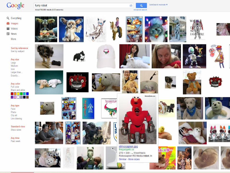

How does Google find furry robots?
(Not the aim of this talk, but we’ll find out…)
Outline
• Motivation
• Proposed flow
• Backgrounder
• Fast Function Extraction (FFX)
• Results
• Conclusion
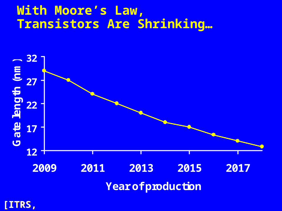
With Moore’s Law, Transistors Are Shrinking…
[ITRS, 2011][ITRS, 2011]
12
17
22
27
32
2009 2011 2013 2015 2017
Year of production
Ga
te l
en
gth
(n
m)
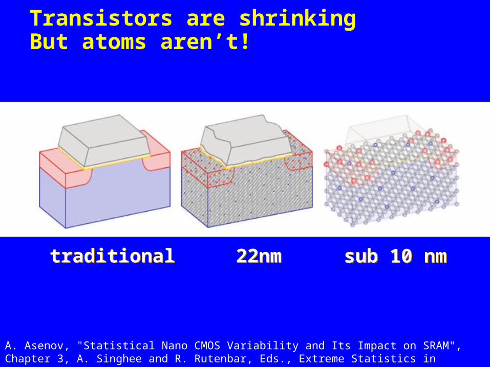
Transistors are shrinkingBut atoms aren’t!
A. Asenov, "Statistical Nano CMOS Variability and Its Impact on SRAM", Chapter 3, A. Singhee and R. Rutenbar, Eds., Extreme Statistics in Nanoscale Memory Design, Springer, 2010
traditionaltraditional 22nm22nm sub 10 nmsub 10 nm
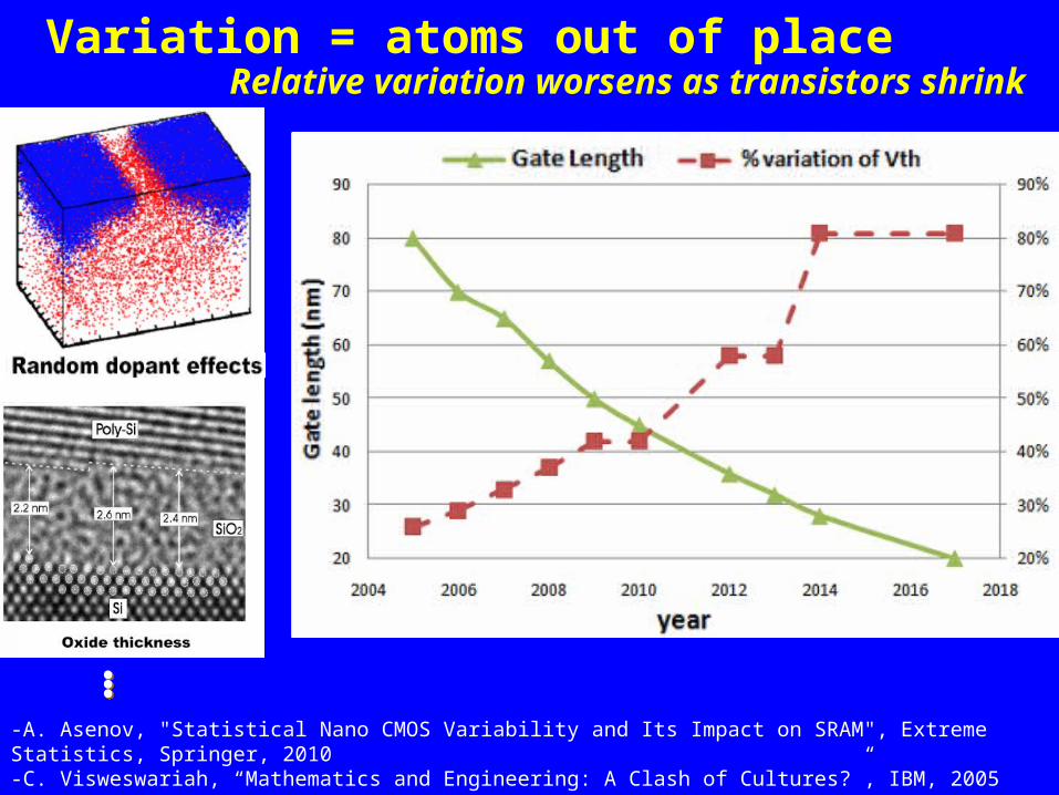
Variation = atoms out of place Relative variation worsens as transistors shrink
-A. Asenov, "Statistical Nano CMOS Variability and Its Impact on SRAM", Extreme Statistics, Springer, 2010-C. Visweswariah, “Mathematics and Engineering: A Clash of Cultures?”, IBM, 2005-ITRS, 2006
……
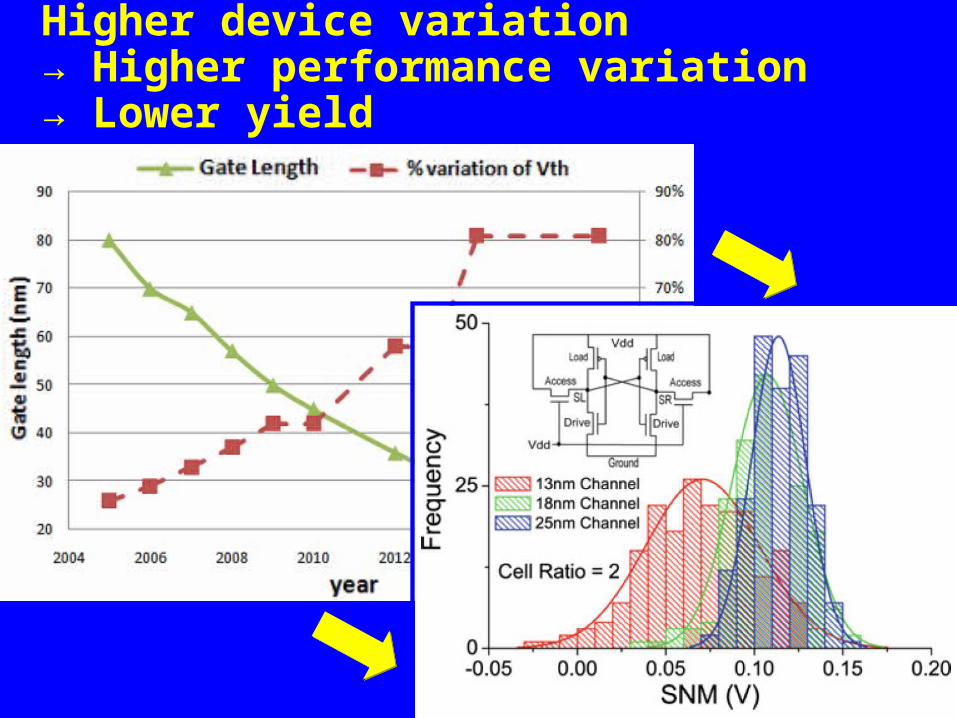
Higher device variation→ Higher performance variation→ Lower yield

Typical Custom Design Flow
(Manual) develop eqns. of design →
performance
(Manual) develop eqns. of design →
performance
Tune sizings forperformance
Tune sizings forperformance
Early-stage design (topology, initial sizing)
Early-stage design (topology, initial sizing)
LayoutLayout……
W1, L1, W2, L2, ..W1, L1, W2, L2, ..
W1, L1, W2, L2, ..W1, L1, W2, L2, ..
F(x)F(x)
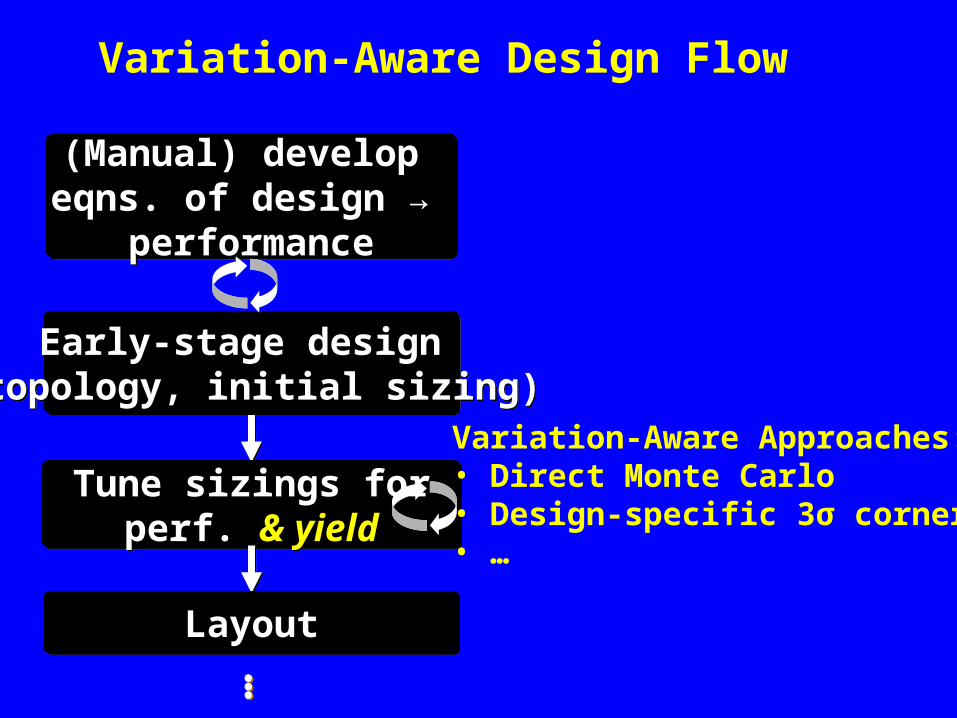
Variation-Aware Design Flow
Tune sizings forperf. & yield
Tune sizings forperf. & yield
Early-stage design (topology, initial sizing)
Early-stage design (topology, initial sizing)
LayoutLayout
……
(Manual) develop eqns. of design →
performance
(Manual) develop eqns. of design →
performance
Variation-Aware Approaches: • Direct Monte Carlo• Design-specific 3σ corners• …

Direct Monte Carlo (MC) For Variation-Aware Design
Early-stage design (topology, initial sizing)
Early-stage design (topology, initial sizing)
LayoutLayout……
(Manual) develop eqns. of design →
performance
(Manual) develop eqns. of design →
performanceSPICE on all 50
(or 1K!) (or 10K!)MC samples
Q: How to get MC out of the design loop, yet retain
accuracy of MC?
Tune sizings forperf. & yieldvia direct MC
Tune sizings forperf. & yieldvia direct MC
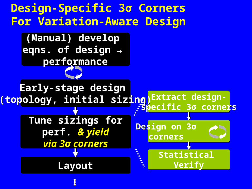
Design-Specific 3σ CornersFor Variation-Aware Design
Extract design-specific 3σ corners
Extract design-specific 3σ corners
Design on 3σ corners
Design on 3σ corners
Statistical Verify
Statistical Verify
Early-stage design (topology, initial sizing)
Early-stage design (topology, initial sizing)
LayoutLayout……
(Manual) develop eqns. of design →
performance
(Manual) develop eqns. of design →
performance
Tune sizings forperf. & yield
via 3σ corners
Tune sizings forperf. & yield
via 3σ corners
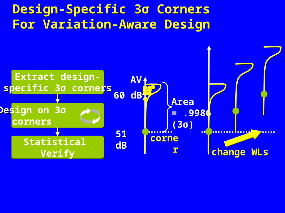
Design-Specific 3σ CornersFor Variation-Aware Design
Extract design-specific 3σ corners
Extract design-specific 3σ corners
Design on 3σ corners
Design on 3σ corners
Statistical Verify
Statistical Verify
AV
51 dB
60 dB
corner
Area = .9986 (3σ)
change WLs

Variation-Aware Design Flow
Tune sizings forperf. & yield
Tune sizings forperf. & yield
Early-stage design (topology, initial sizing)
Early-stage design (topology, initial sizing)
LayoutLayout
……
(Manual) develop eqns. of design →
performance
(Manual) develop eqns. of design →
performanceThere are effective
industrial-scale
methods here…
…butnot
here
This paperaims to help!

Outline
• Motivation
• Proposed flow
• Backgrounder
• Fast Function Extraction (FFX)
• Results
• Conclusion

An Ideal Flow
Tune sizings forperf. & yield
Tune sizings forperf. & yield
Early-stage design (topology, initial sizing)
Early-stage design (topology, initial sizing)
LayoutLayout……
(Manual) develop eqns. of design & process vars.
→ circuit performance
(Manual) develop eqns. of design & process vars.
→ circuit performance
“Dear designer,To handle
mismatch in early design stages,
please add 1000 extra variables
∆tox1, ∆Nsub1, …∆tox100, ∆Nsub100,
…”
Are you an expert at process modeling?
Who is an expert at both process modeling
& topology development?
… Is Infeasible
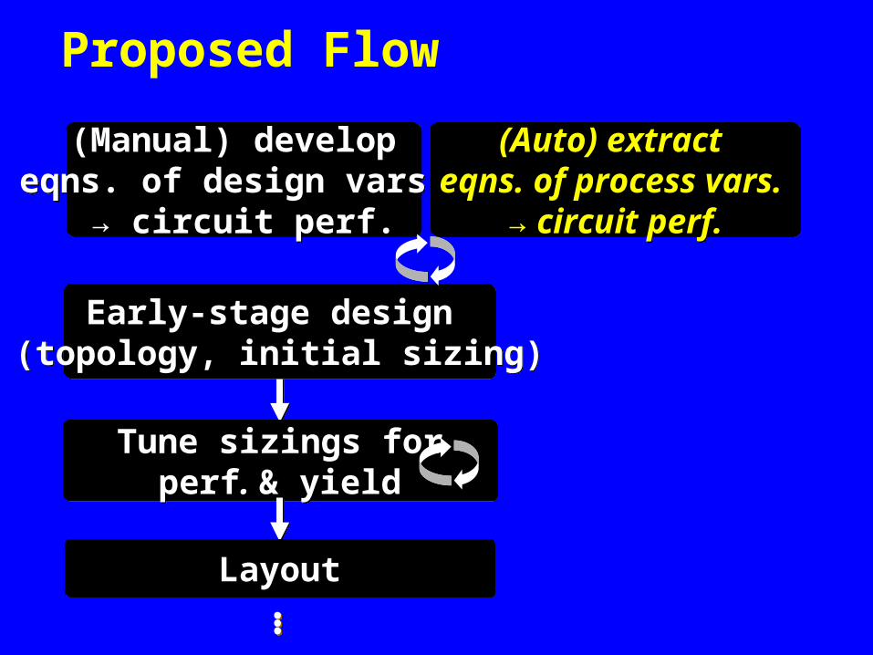
Proposed Flow
Tune sizings forperf. & yield
Tune sizings forperf. & yield
Early-stage design (topology, initial sizing)
Early-stage design (topology, initial sizing)
LayoutLayout……
(Manual) develop eqns. of design vars.
→ circuit perf.
(Manual) develop eqns. of design vars.
→ circuit perf.
(Auto) extract eqns. of process vars.
→ circuit perf.
(Auto) extract eqns. of process vars.
→ circuit perf.

Equation-Extraction Step: Details, by Example (1D)
Draw 100-5000 MCsamples (X)
Draw 100-5000 MCsamples (X)
SPICE-Simulate onsamples (y)
SPICE-Simulate onsamples (y)
∆tox1 (X)
AV(y)
AV
∆tox1
AV=50.2 + 9.1 • ∆tox1 + 3.2 • max(0, ∆tox12)
∆tox1
Build whiteboxModel of X → yBuild whiteboxModel of X → y
sim.

Equation-Extraction Step: Problem Scope
• 5-10+ process variables per device
(e.g. BPV model)
• 10-100+ devices
• Therefore 50-1000+ input variables
• 100-5000 simulations (runtime cost)
• Need whitebox model, for insight!
• Ideally get a tradeoff of complexity vs. accuracy

Equation Extraction Step:Off-the-Shelf Modeling Options
• Linear model – can’t handle nonlinear
• Quadratic – not nonlinear enough, scaling?
• MARS, SVM, neural net, others – not whitebox
Nothing meets problem scope!

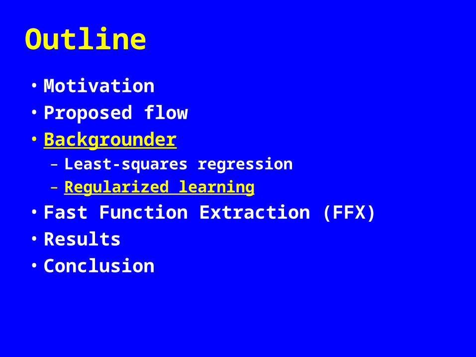
Outline
• Motivation• Proposed flow• Backgrounder
– Least-squares regression– Regularized learning
• Fast Function Extraction (FFX)• Results• Conclusion
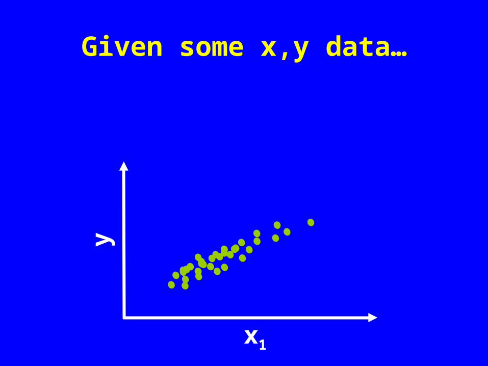
Given some x,y data…
x1
y
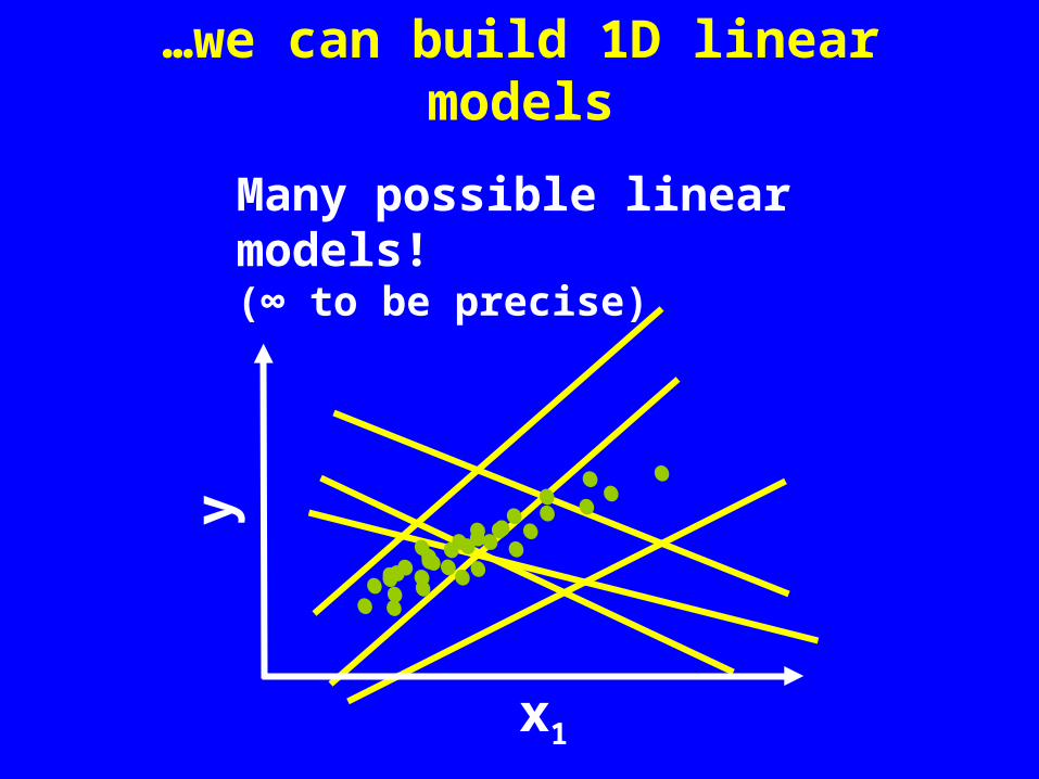
…we can build 1D linear models
Many possible linear models! (∞ to be precise)
x1
y

1D Linear Least-Squares (LS) Regression
x1
y
Find linear model that minimizes ∑(ŷi-yi)2
(across all i in training data)
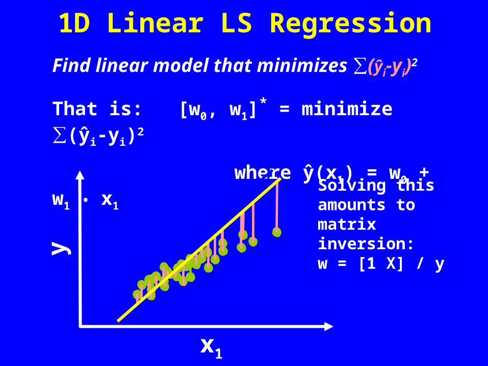
1D Linear LS Regression
Find linear model that minimizes ∑(ŷi-yi)2
That is: [w0, w1]* = minimize ∑(ŷi-yi)2
where ŷ(x1) = w0 + w1 • x1
x1
y
Solving this amounts to matrix inversion: w = [1 X] / y

1D Quadratic LS Regression[w0, w1, w11]
* = minimize ∑(ŷi-yi)2
where ŷ(x1) = w0 + w1 • x1 + w11 • x12
We are applying linear (LS) learning on linear & nonlinear basis functions. OK!
x1
y

1D Nonlinear LS Regression[w0, w1, wsin]
* = minimize ∑(ŷi-yi)2
where ŷ(x1) = w0 + w1 • x1 + wsin • sin(x1)
We are applying linear (LS) learning on linear & nonlinear basis functions. OK!
x1
y

2D Linear LS Regression
[w0, w1, w2]* = minimize ∑(ŷi-yi)2
where ŷ(x) = w0 + w1 • x1 + w2 • x2
y
x 1
x2

2D Quadratic LS Regression[w0, w1, w2, w11, w22, w12]
* = minimize ∑(ŷi-yi)2
where ŷ(x) = w0 + w1 • x1 + w11 • x12 + w22 • x2
2 + w12 • x1 • x2
x1
x2
y
Outline
• Motivation• Proposed flow• Backgrounder
– Least-squares regression– Regularized learning
• Fast Function Extraction (FFX)• Results• Conclusion

Regularized Linear Regression
• Minimizes a combination of training error and model sensitivity
• Formulation:w* = minimize ( ∑(ŷi(w) - yi)2 + λ • ∑|wj| )
minimize training error (fit training data better)
model sensitivity(reduce risk in future predictions)
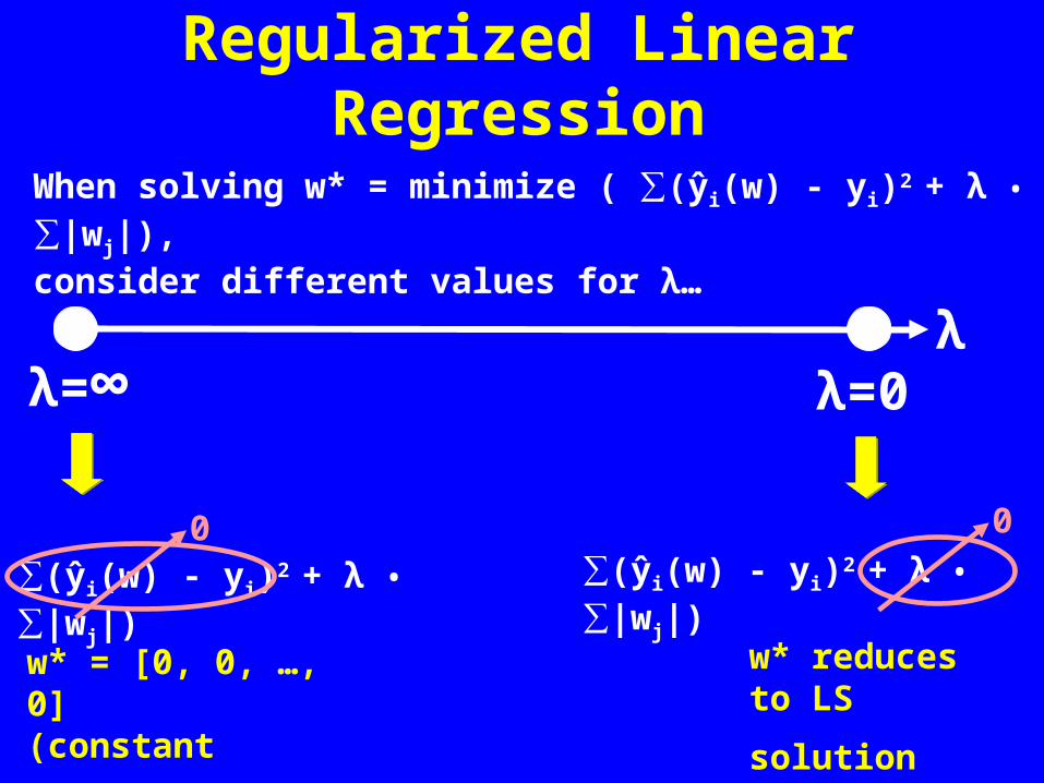
Regularized Linear Regression
λ=∞ λ=0λ
∑(ŷi(w) - yi)2 + λ • ∑|wj|)∑(ŷi(w) - yi)2 + λ • ∑|wj|)
00
w* reduces to
LS solution w* = [0, 0, …, 0]
(constant response)
When solving w* = minimize ( ∑(ŷi(w) - yi)2 + λ • ∑|wj|), consider different values for λ…

Pathwise Regularized Linear Regression
solve w* = minimize ( ∑(ŷi(w) - yi)2 + λ • ∑|wj|)
at λ=1e40 (λ→∞)
λ λ=1e-40
wi
w* = [0, 0, 0, 0]
λ=1e40

Pathwise Regularized Linear Regression
solve w* = minimize ( ∑(ŷi(w) - yi)2 + λ • ∑|wj|) at λ=1e30
wi
w1,3,4
w* = [0, 1.8, 0, 0]
w2
λ λ=1e-40
λ=1e30

Pathwise Regularized Linear Regression
solve w* = minimize ( ∑(ŷi(w) - yi)2 + λ • ∑|wj|) at λ=1e20
wi w* = [0, 2.8, 0, 0]
λ λ=1e-40
λ=1e20
w2
w1,3,4

Pathwise Regularized Linear Regression
solve w* = minimize ( ∑(ŷi(w) - yi)2 + λ • ∑|wj|) at λ=1e10
wi w* = [-0.5, 2.8, 0, 0]
λ λ=1e-40
λ=1e10
w2
w1
w3,4

Pathwise Regularized Linear Regression
solve w* = minimize ( ∑(ŷi(w) - yi)2 + λ • ∑|wj|) at λ=1e0
wi w* = [-0.5, 2.8, 0, 0]
λ λ=1e-40
λ=1e0
w2
w1
w3,4
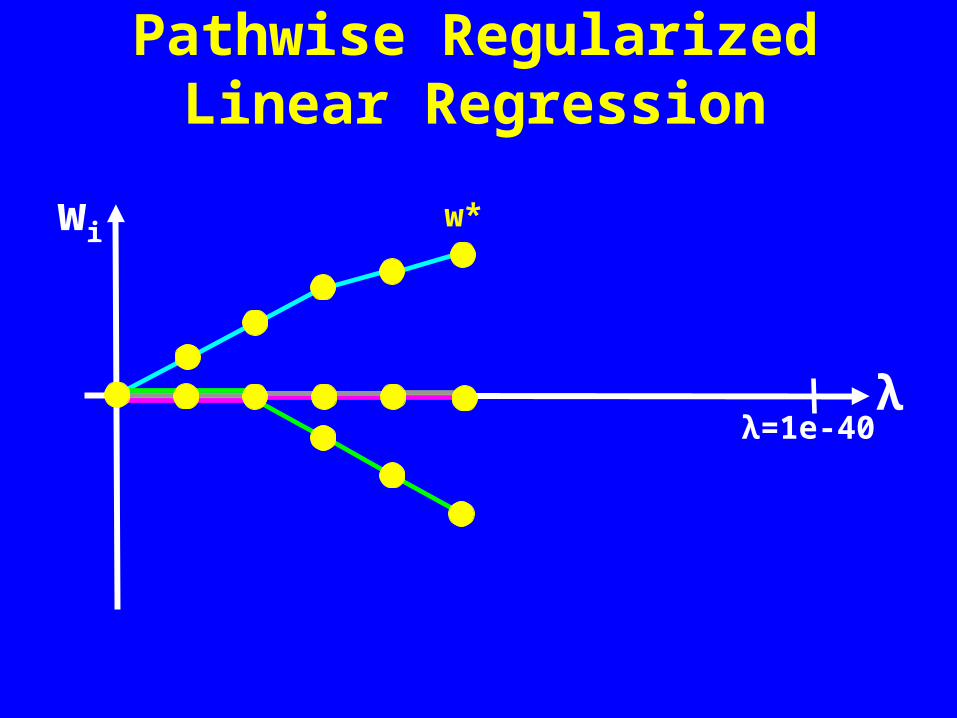
Pathwise Regularized Linear Regression
wi
λ λ=1e-40
w*

Pathwise Regularized Linear Regression
wi
λ λ=1e-40
w*

Pathwise Regularized Linear Regression
wi
λ
w* = [-3.5, 2.9, 0.6, -1.4]

Pathwise Regularized Linear Regression
wi
λ
Each column vector of w* is a different linear model.Which model is better / best? Accuracy vs. complexity…
w*

Pathwise RegressionAccuracy Per Model
wi λ
Training error∑(ŷi(w) - yi)2
for training i
Test error∑(ŷi(w) - yi)2
for test i overfitting
one model
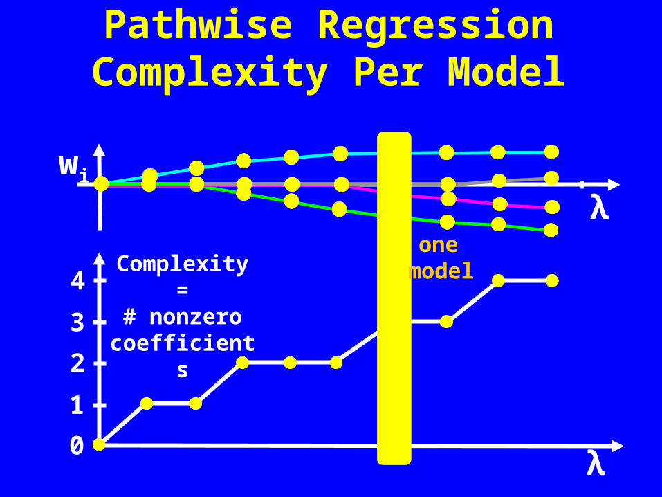
Pathwise RegressionComplexity Per Model
wi λ
Complexity =# nonzero
coefficients
0λ
1
2
3
4
one model

Accuracy – Complexity Tradeoff
# nonzero coefficients)
λ
Test error
Test error
# nonzero coeffs.
λ
Ideal
Tradeoff
+
=
one model

Cool Propertiesof Pathwise Regression
(versus plain old LS)
• Cool property #1: solving a full regularized path gives us accuracy-vs-complexity tradeoffs!
• Cool property #2: can have more coefficients than samples!
• Regularization term ∑|wi| means no underdetermined problems
• Cool property #3: solving a regularized learning problem is just as fast (or faster) than solving a least-squares learning problem!
• Why: convex optimization problem – one big hill

Q: How does Google find furry robots?
Answer (NIPS 2010):1. Treat images as 1000x1000 = 1M input vars. (x)
2. Crawl the web:• Find all images with “furry” & “robot” in filename.
Assign y-value = 1.0• Find ≤5K images with “furry”, “robot”. y-value = 0.75• Randomly grab 5K more images. y-value = 0.0
3. Run regularized linear learning on X → y (learning on 1M input variables!!)
4. On all unseen images, run model. Return images sorted from highest ŷ down.
• Cool property #4: regularized learning can handle a ridiculous number of input variables!

Outline
• Motivation• Proposed flow• Backgrounder
– Least-squares regression– Regularized learning
• Fast Function Extraction (FFX)• Results• Conclusion
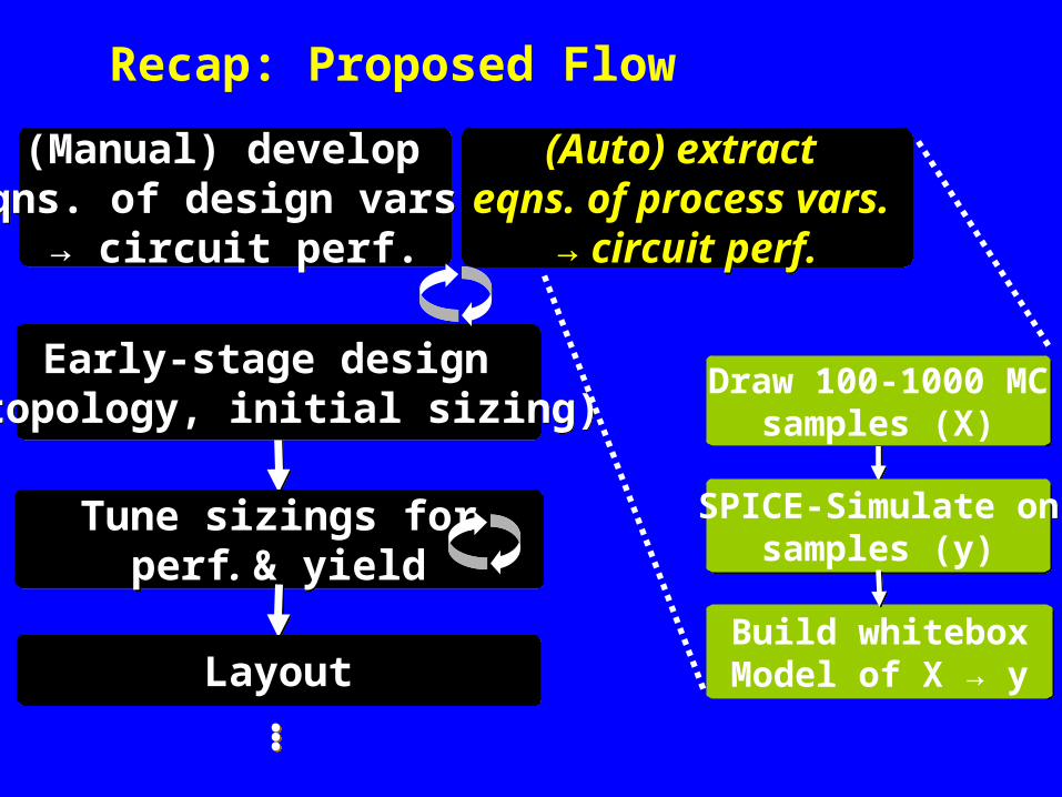
Recap: Proposed Flow
Tune sizings forperf. & yield
Tune sizings forperf. & yield
Early-stage design (topology, initial sizing)
Early-stage design (topology, initial sizing)
LayoutLayout
……
(Manual) develop eqns. of design vars.
→ circuit perf.
(Manual) develop eqns. of design vars.
→ circuit perf.
(Auto) extract eqns. of process vars.
→ circuit perf.
(Auto) extract eqns. of process vars.
→ circuit perf.
Draw 100-1000 MCsamples (X)
Draw 100-1000 MCsamples (X)
SPICE-Simulate onsamples (y)
SPICE-Simulate onsamples (y)
Build whiteboxModel of X → yBuild whiteboxModel of X → y
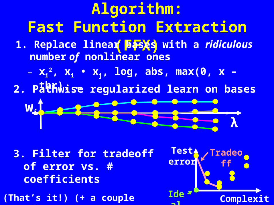
A New Modeling Algorithm:Fast Function Extraction (FFX)
1. Replace linear bases with a ridiculous number of nonlinear ones
– xi2, xi • xj, log, abs, max(0, x – thr), …
3. Filter for tradeoff of error vs. # coefficients
2. Pathwise regularized learn on bases
Test error
ComplexityIdeal
Tradeoff
wi λ
(That’s it!) (+ a couple tweaks)

Outline
• Motivation
• Proposed flow
• Backgrounder
• Fast Function Extraction (FFX)
• Results
• Conclusion

Circuit Test ProblemsCircuit #
Devices# Process
Vars.Outputs Modeled
Opamp 30 215 AV (gain), BW (bandwidth), PM (phase margin), SR (slew rate)
Bitcell 6 30 celli (read current)
Sense amp
12 125 delay, pwr (power)
Voltage ref.
11 105 DVREF (difference in voltage), PWR (power)
GMC filter
140 1468 ATTEN (attenuation), IL
Comp-arator
62 639 BW (bandwidth)
HspiceTM, industrial MOS models < 65nm, 800-5K MC samples
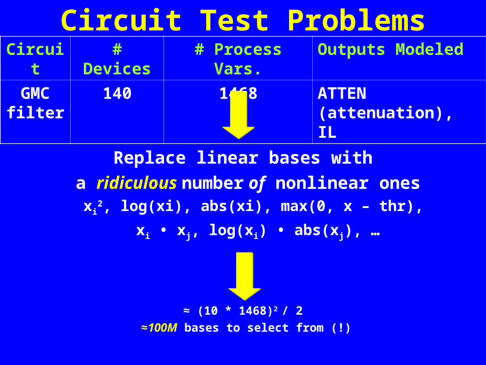
Circuit Test ProblemsCircuit # Devices # Process Vars. Outputs Modeled
GMC filter
140 1468 ATTEN (attenuation), IL
Replace linear bases with
a ridiculous number of nonlinear onesxi
2, log(xi), abs(xi), max(0, x – thr),
xi • xj, log(xi) • abs(xj), …
≈ (10 * 1468)2 / 2
≈100M bases to select from (!)

Circuit Test ProblemsCircuit #
Devices# Process
Vars.Outputs Modeled
Opamp 30 215 AV (gain), BW (bandwidth), PM (phase margin), SR (slew rate)
Bitcell 6 30 celli (read current)
Sense amp
12 125 delay, pwr (power)
Voltage ref.
11 105 DVREF (difference in voltage), PWR (power)
GMC filter
140 1468 ATTEN (attenuation), IL
Comp-arator
62 639 BW (bandwidth)
Results summary: <30 s build time. Error always < linear & quadratic, sometimes dramatically.

Opamp PM Equations (215 global + local process variables. Modeling time < 30 s)
# bases
Test
error
Extracted Equation
0 15.5 % 59.6
1 6.8 59.6 – 0.303 • dxl
2 6.6 59.6 – 0.308 • dxl – 0.00460 • cgop
3 5.4 59.6 – 0.332 • dxl – 0.0268 • cgop + 0.0215 • dvthn
4 4.2 59.6 – 0.353 • dxl – 0.0457 • cgop + 0.0211 • dvthn – 0.0211 • dvthp
5 4.1 59.6 – 0.354 • dxl – 0.0460 • cgop + 0.0198 • dvthn – 0.0217 • dvthp + 0.0135 • abs(dvthn) • dvthn
… …
46 1.0 58.9 – 0.136 • dxl + 0.0299 • dvthn – 0.0194…
Opamp PM Equations Visualize Accuracy-Complexity Tradeoff

Voltage Ref. DVREF Equations (105 global + local process variables. Modeling time < 30 s)
# bases
Test
error
Extracted Equation
0 2.6 % 512.7
1 2.1 504 / (1.0 + 0.121 • max(0, dvthn + 0.875))
… … …
8 0.9 476 / (1.0 + 0.105 • max(0, dvthn + 1.61) – 0.0397 • max(0, -1.64 – dvthp) + …)
Shows: FFX is highly nonlinear if needed

Global vs. Local Variation?
# bases
Test
error
Opamp PM Extracted Equation
3 5.4 59.6 – 0.332 • dxl – 0.0268 • cgop + 0.0215 • dvthn
local (mismatch) variables
# bases
Test
error
Comparator BW Extracted Equation
3 18.1 171e6 – 4.57e5 • xcm1,m1,lint • xcm1,m2,lint
+ 5.23e4 • x2cm1,m1,lint + 4.80e4 • x2
cm1,m2,lint
global process variables
FFX uses whatever variables help most, and sometimes patterns emerge

Highest-Impact Variables for Opamp PM % Impact Variable Name
46.5 dxl
10.2 cgop
9.7 dvthn
7.4 dvthp
3.9 RCN_nsmm_DXL
3.8 RCP_nsmm_DXL
3.6 dxw
3.1 cgon
2.3 RCP_nsmm_DXW… …
0.3 CM1_M1_nsmm_LINT
0.3 CMB2_M1_nsmm_NSUB… …
Outline
• Motivation
• Proposed flow
• Backgrounder
• Fast Function Extraction (FFX)
• Results
• Conclusion

Conclusion• Process variation is bad, and getting worse• There are solutions for design tuning
… But not for early-stage manual topology design
• Idea: complement hand-derived equations with auto-extracted equations of variation → performance
• FFX builds the models (fast, scalable, nonlinear)
…with the help of pathwise regularized learning
• Easy to get started: code at trent.st/FFX– Just ≈3 pages of python!– Solido using it extensively. Others too, for analog
test, behavioral modeling, and even web search (!)