High-Accuracy GPS Semikinematic Positioning: Modeling and ...

NAvlC.vno~: Journal of The Institute ofNavigation

Vol. 37, No. 1, Spring 1990

Rinted in U.S.A.

High-Accuracy GPS Semikinematic Positioning: Modeling and Results

M. ELIZABETH CANNON

The University of Calgary, Calgary, Alberta, Canada Received September 1989 Revised November 1989

ABSTRACT

The concept of GPS semikinematic positioning is reviewed, with an emphasis on accuracies at the centimeter level. Details of the mathematical model used herein are given. A two-step approach combines a Kalman filter to process kinematic carrier phase, phase rate, and pseudorange data, while a batch least-squares adjustment processes static carrier phase data. A semikinematic test performed over a well-controlled traverse in a mountainous region near Calgary is used to assess the performance of the algorithm. Several runs of the traverse were made with the station occupation time at 2-3 min. The analysis shows that centimeter-level accuracies can be achieved when five satellites are observed in good geometery, even when frequent cycle slips occur. An accuracy improvement technique of reverse processing is also investigated. Recommendations for improving semikinematic surveying are made.

INTRODUCTION

GPS semikinematic positioning is a procedure in which stations along a traverse are occupied for a short time, e.g. 2-4 min, and then the receiver is moved to the next station along the traverse. The name semikinematic refers to the two dynamic states of the receiver; part of the time is spent static on a station, while the rest of the time the receiver is in pure kinematic mode en route to the next station. This method is an extension of conventional GPS relative static surveying, which normally requires l-2 h of data per station to obtain centimeter accuracy. The goal of semikinematic surveying is to maintain the centimeter-level accuracy while reducing the site occupation time from hours to minutes. By achieving this goal, dramatic cost and time savings can be made on a precise GPS survey. One application of the semikinematic technique is for densification of control points in geodetic networks.

A number of semikinematic tests have been performed to date, for example, those described in [l-6]. Centimeter accuracies have been achieved under varying conditions, ranging from very short baselines, for example, as described in [5 and 61, to baselines of up to 20 km [21. Most of the processing techniques do not use the kinematic GPS data collected between the static stations. A method is presented in this paper which uses both the static and kinematic data in a two-step processing technique. A least-squares batch adjustment is used to process the static data, while a Kalman filter is implemented on

53

54 Navigation Spring 1990

the kinematic data. Also presented is a procedure of reverse-processing for accuracy improvement over semikinematic runs with accuracy degradation due to cycle slips.

MATHEMATICAL MODEL

Two methods are used for postprocessing of GPS data. A batch least-squares adjustment of double-differenced carrier phase is used to process the 2-3 min of static data, while a Kalman filter is implemented during the kinematic secti0n.s between static points. Data used in the Kalman filter include carrier phase data, as well as phase rate and pseudoranges. All measurements input to the Kalman filter are processed using double differencing. The advantage of using this approach as opposed to processing only static data is that no information is neglected. By processing kinematic data, information on cycle slip occur- rence is gained. New carrier phase ambiguities can then be estimated during transit to the next station.

Static Rata Processing Model

The GPS carrier phase data collected at static stations were processed using a batch least-squares adjustment. Details of the double-difference method are not given here, but can be found in 171. The basic observation equation between two receivers and two satellites is 181:

VA+ = VAp + XVAN - VAdi,,,, + VAd,,, + Vhd, + E (1)

where VA denotes double difference, + is the carrier phase observation (m), p is the range between a satellite and receiver (m), A is the carrier phase wavelength (m), N is the carrier phase integer ambiguity (cycles), dion is the ionospheric correction (m), drop is the tropospheric correction (m), d, is the orbital error (m), and E is the measurement noise (m). Ionospheric and tropospheric corrections are not applied to the observations since the baselines are less than 10 km.

At the first station of the traverse, the baseline, i.e., the vector between the differential GPS monitor and remote receivers, was held fixed in order to estimate the carrier phase integer ambiguities. This assumes that the baseline is known a priori. If this is not the case, techniques such as antenna swapping 191 or a conventional static solution (i.e., longer observation span) could be implemented. After this first static solution is performed, the estimated remote receiver coordinates from the adjustment, along with their variances, are entered as a priori information into the Kalman filter. The integer ambiguities are stored, but are generally not estimated in the Kalman filter, as discussed in the next section.

In processing subsequent stations along the traverse, the ambiguities are estimated only if a cycle slip has occurred since the last static point. If no cycle slips have occurred, the ambiguities are held fixed to their previous integer values, and only station coordinates are estimated. Knowledge of the integer ambiguities in semikinematic positioning is crucial for maintaining centimeter-level accuracy, since 2-3 min of static data is then sufficient to determine precise station coordinates. In conventional GPS static differential surveys,

Vol. 37, No. 1 Cannon: GPS Semikinematic Positioning 55

a longer data span is necessary in order to accumulate sufficient geometric information to resolve the integer ambiguity parameters.

If cycle slips occur during the kinematic section, new carrier phase integer ambiguities for those satellites affected are estimated in the next static least- squares adjustment. In order to constrain the ambiguities somewhat, a priori information on the ambiguities is taken from the Kalman filter results. Clearly, the more accurate the a priori information input to the least-squares adjustment, the stronger the possibility of recovering the new carrier phase integer ambiguity.

Kinematic Data Processing Model

A Kalman filter is implemented to process the kinematic GPS data collected between stations. The underlying theory can be found in [lo]. Measurements used to update the Kalman filter are differential carrier phase, phase rates, and pseudoranges. Phase rates are included to improve velocity determination, while pseudoranges assist in bounding the error during periods of multiple cycle slips. Both these measurement types improve the filter performance, especially the phase rates since they contribute to the modeling of the vehicle dynamics. All measurements are processed in double-difference mode. Stan- dard deviations of 0.5 cm, 5 cm/s, and 4 m are applied to the double-differenced carrier phase, phase rates, and pseudoranges, respectively.

The state vector, x, of the filter is

x = (64, ah, ah, 8v,, Sv,, 6~“)~ (2)

where S+ is the correction to latitude, 6h is the correction to longitude, Sh is the correction to height, 6v, is the correction to north velocity, 6v, is the correction to east velocity, and 6v, is the correction to up velocity.

Equation (2) gives the state vector if carrier phase ambiguities have been resolved to their integer values. In this case, there is no need for carrier phase ambiguity estimation. However, if cycle slips occur during a kinematic section, the state vector is augmented to estimate the ambiguities that have been affected. The augmented state vector is

X = (64, ah, 6h, 6V,, 8V,, 8V”, 6Ni,..., 6Nj}T (3)

where 6N is the magnitude of a satellite’s carrier phase ambiguity, and j is the number of satellites that have had cycle slips. Cycle slips are detected by comparing the measured carrier phase measurement to the predicted measurement using the measured phase rate.

The Kalman filter prediction and update equations as given in 1101 are listed below:

Prediction: % k+ I ( - ) = *k+ I,&

c E+1 (-) = %+I& ~fi@,T+,,lc+c~+l,k

Update: x(+) = %(-) + K {I-A%(-)}

P(+) = {I-KA} w-1

K = C”( - )AT {AC”( - )AT + cF}-1

(4a)

(4b)

(4c)

(4d)

(4e)


where & is the estimated state vector, Q, is the transition matrix, C” is the state covariance matrix, C” is theprocess noise matrix, K is the Kalman gain matrix, 1 is the observations, A is the design matrix, and C” is the measurement noise matrix. The (- ) and ( + ) represent estimates before and after measurement update, respectively.

Each kinematic section is initialized with position and covariance information from the double-difference solution. When a cycle slip occurs, the state vector is augmented by the carrier phase ambiguity term. At the next static station, this ambiguity is estimated in the least-squares double-difference adjustment. Ideally, using the a priori information from the Kalman filter, the new integer ambiguity is resolved. If the proper combination of integer ambiguities cannot be reliably resolved during the adjustment, the Kalman state vector is kept augmented for the next kinematic section.

This relationship of feeding information back and forth from the Kalman filter a.nd least-squares adjustment exploits the use of all the data collected. Some semikinematic processing techniques, for example, those described in 13-51, do not process data between static points. However, as will be shown, use of the technique described above allows cycle slips to be identified when they occur and estimated during transit.

SEMIKINEMATIC TEST DESCRIPTION

Semikinematic tests were performed in August 1988, in the Kananaskis region, located approximately 80 km west of Calgary. An 8 km stretch of highway was selected as the test traverse. A control station was established every kilometer along the road using precise static GPS techniques. The result- ing 8 points are known with an accuracy of 2-5 cm with respect to the monitor station, located less than 1 km from the first control point.

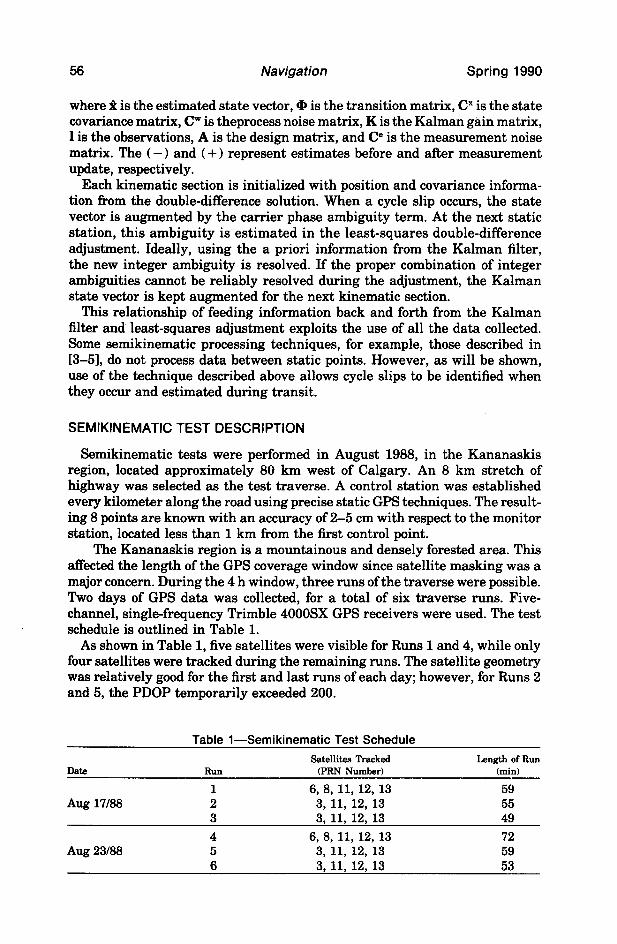
The Kananaskis region is a mountainous and densely forested area. This affected the length of the GPS coverage window since satellite masking was a major concern. During the 4 h window, three runs of the traverse were possible. Two days of GPS data was collected, for a total of six traverse runs. Five- channel, single-frequency Trimble 4000SX GPS receivers were used. The test schedule is outlined in Table 1.

As shown in Table 1, five satellites were visible for Runs 1 and 4, while only four satellites were tracked during the remaining runs. The satellite geometry was relatively good for the first and last runs of each day; however, for Runs 2 and 5, the PDOP temporarily exceeded 200.

Table 1-Semikinematic Test Schedule

Satellites Tracked Length of Run Date Run (PRN Number) bin)

1 6, 8, 11, 12, 13 59 Aug 17188 2 3, 11, 12, 13 55

3 3, 11, 12, 13 49

4 6, 8, 11, 12, 13 72 Aug 23188 5 3, 11, 12, 13 59

6 3, 11, 12, 13 53


A tripod was set up on each control station before the test began, and each antenna height was measured. This was done to save time during the actual survey. At each stop, the antenna had to be mounted manually on the tripod. Since these tests were performed, a mobile lever has been developed which holds the antenna. Once mounted on a vehicle roof, the lever can be swung out so the antenna can be centered directly over the point.

The first station of the traverse was occupied for lo-15 min. While still logging GPS data, the vehicle was then driven at about 50 km/h to the next station. The second and subsequent stations were occupied for 2-3 min. Cycle slips were detected during kinematic sections of the traverse when the satellite signal was shaded because of the mountains and trees. Although it was appar- ent from the data-logging computer output that cycle slips were occurring, no additional procedures were invoked in the field to counteract their effect.

DISCUSSION OF RESULTS

The data were postprocessed using the program SEMIKIN, developed by the author at The University of Calgary. It implements the two-step model detailed above and runs automatically without operator intervention once an input file has been created. It was developed in FORTRAN on a VAXJVMS computer, but has since been installed on a Compaq 386 portable computer for field use. Future plans include translating the software to the C language.

Only four of the six semikinematic runs were processed since satellite masking was a severe problem during the second run of each day. The semikinematic results at each of the static stations were compared to the control coordinates independently determined for each station. Unfortunately, no control information was available during the kinematic sections of the traverse.

Forward Processing

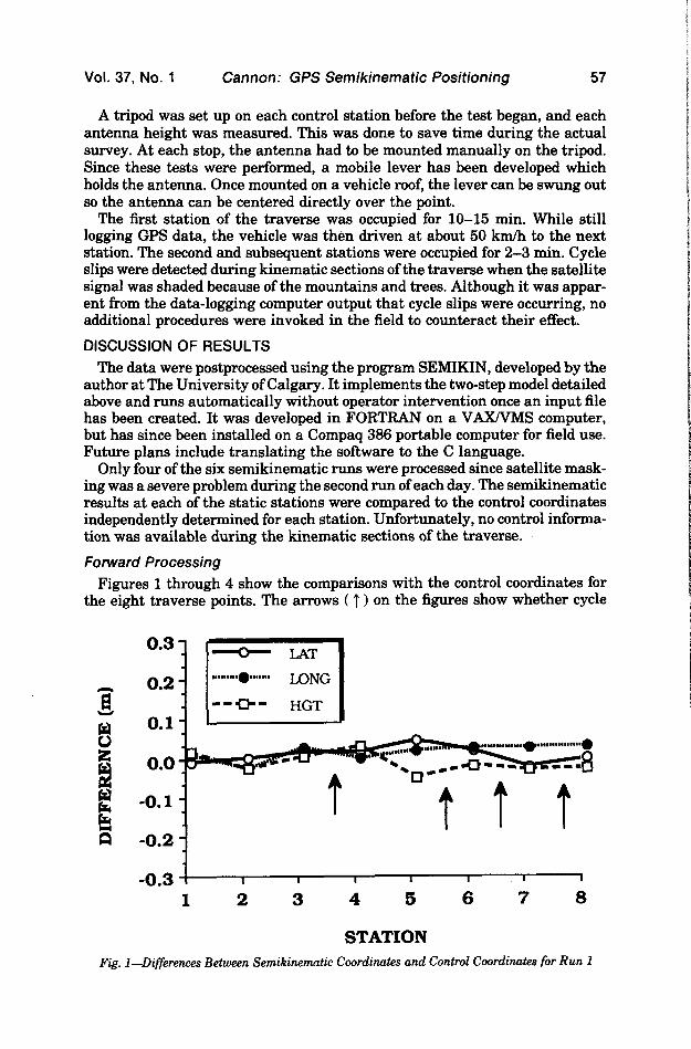
Figures 1 through 4 show the comparisons with the control coordinates for the eight traverse points. The arrows ( t ) on the figures show whether cycle

8

:

2 E Ei

Fig. 1.

-0.3 ; I I I I I I 1

1 2 3 4 5 6 7 8

STATION

-Differences Between Semikinematic Coordinates and Control Coordinates for Run 1


0.3 1

0.1-I .o

0.0

-0.1

-0.2

STATION

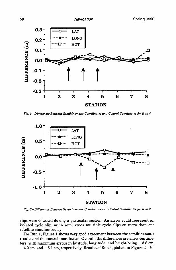
Fig. Z-Differences Between Semikinematic Coordinates and Control Coordinates for Run 4

-0.5 -

-1.0 I I I I I I I 1 1 2 3 4 5 6 7 8

STATION

Fig. J-Differences Between Semikinematic Coordinates and Control Coordinates for Run 3

slips were detected during a particular section. An arrow could represent an isolated cycle slip, or in some cases multiple cycle slips on more than one satellite simultaneously.

For Run 1, Figure 1 shows very good agreement between the semikinematic results and the control coordinates. Overall, the differences are a few centimeters, with maximum errors in latitude, longitude, and height being - 3.6 cm, - 4.0 cm, and - 6.1 cm, respectively. Results of Run 4, plotted in Figure 2, also


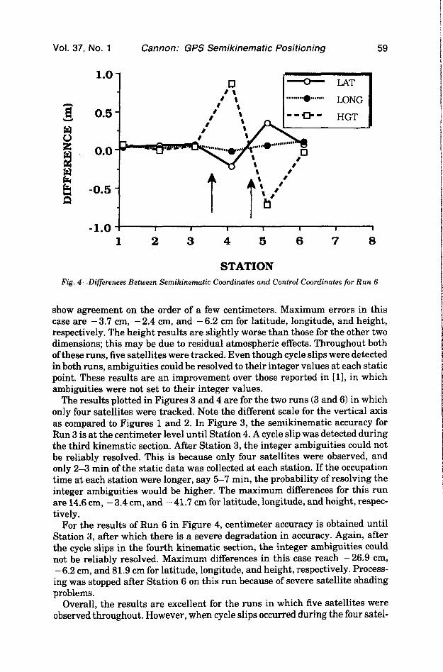
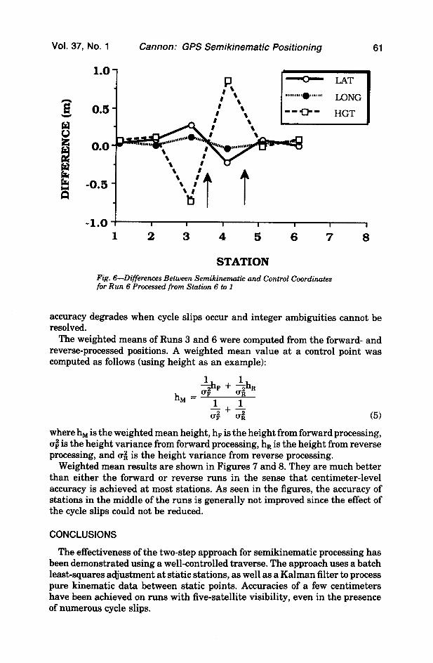
Fig. I-Differences Between Semikinematic Coordinates and Control Coordinates for Run 6

show agreement on the order of a few centimeters. Maximum errors in this case are - 3.7 cm, - 2.4 cm, and - 6.2 cm for latitude, longitude, and height, respectively. The height results are slightly worse than those for the other two dimensions; this may be due to residual atmospheric effects. Throughout both of these runs, five satellites were tracked. Even though cycle slips were detected in both runs, ambiguities could be resolved to their integer values at each static point. These results are an improvement over those reported in [l], in which ambiguities were not set to their integer values.

The results plotted in Figures 3 and 4 are for the two runs (3 and 6) in which only four satellites were tracked. Note the different scale for the vertical axis as compared to Figures 1 and 2. In Figure 3, the semikinematic accuracy for Run 3 is at the centimeter level until Station 4. A cycle slip was detected during the third kinematic section. After Station 3, the integer ambiguities could not be reliably resolved. This is because only four satellites were observed, and only 2-3 min of the static data was collected at each station. If the occupation time at each station were longer, say 5-7 min, the probability of resolving the integer ambiguities would be higher. The maximum differences for this run are 14.6 cm, - 3.4 cm, and - 41.7 cm for latitude, longitude, and height, respectively.

For the results of Run 6 in Figure 4, centimeter accuracy is obtained until Station 3, after which there is a severe degradation in accuracy. Again, after the cycle slips in the fourth kinematic section, the integer ambiguities could not be reliably resolved. Maximum differences in this case reach -26.9 cm, - 6.2 cm, and 81.9 cm for latitude, longitude, and height, respectively. Process- ing was stopped after Station 6 on this run because of severe satellite shading problems.

Overall, the results are excellent for the runs in which five satellites were observed throughout. However, when cycle slips occurred during the four satel-


lite runs, the integer ambiguities could not be reliably resolved after cycle slips. This is due to the lack of redundancy and will not occur once the full constellation is in place.

Improving Results by Reverse Processing

In order to improve results for Runs 3 and 6, the data was processed in reverse time, that is, starting at Station 8 (Station 6 in the case of Run 6) and ending at Station 1. Combining the estimated positions of forward processing and reverse processing should result in a better weighted position. This stems from the fact that the semikinematic coordinate accuracy is very good until cycle slips occur. If they occur during the middle of a run, the results of the remaining stations can be affected, as seen in Figures 3 and 4. Processing the data in reverse should at least improve the stations at the end of the forward run (i.e., the beginning of the reverse run). This technique was not applied to Runs 1 and 4 since the ambiguities were resolved to their integer values during the forward processing. However, processing a traverse in reverse gives a measure of the reliability of the results.

The same two-step static and kinematic methodology described earlier was used to process the data in reverse. The coordinates of Station 8 (Station 6 for Run 6) were held fixed to determine the initial “reverse” integer ambiguities. This assumes that the coordinates of the end station of the traverse are known, or that the traverse is closed at the first station. Alternatively, a conventional static survey could be performed at the last station of the traverse.

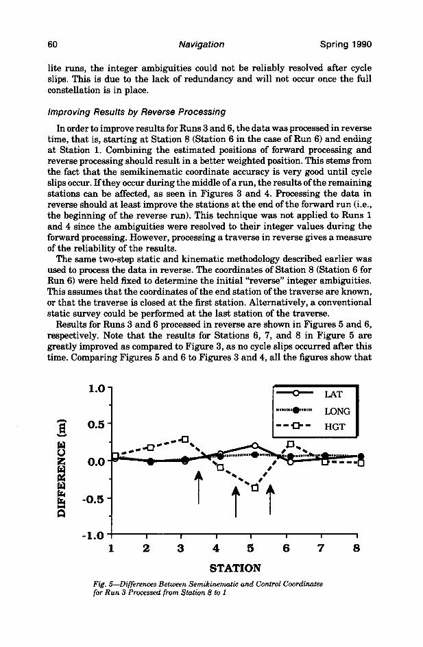
Results for Runs 3 and 6 processed in reverse are shown in Figures 5 and 6, respectively. Note that the results for Stations 6, 7, and 8 in Figure 5 are greatly improved as compared to Figure 3, as no cycle slips occurred after this time. Comparing Figures 5 and 6 to Figures 3 and 4, all the figures show that

1.0 -

-1.0 I I I I I I I

1 2 3 4 5 6 7 8

STATION

Fig. 5-Differences Between Semikinematic and Control Coordinates for Run 3 Processed from Station 8 to 1


-1.0 ,’ I I I I I I I

1 2 3 4 5 6 7 8

STATION

Fig. &Differences Between Semikinematic and Control Coordinates for Run 6 Processed from Station 6 to 1

accuracy degrades when cycle slips occur and integer ambiguities cannot be resolved.

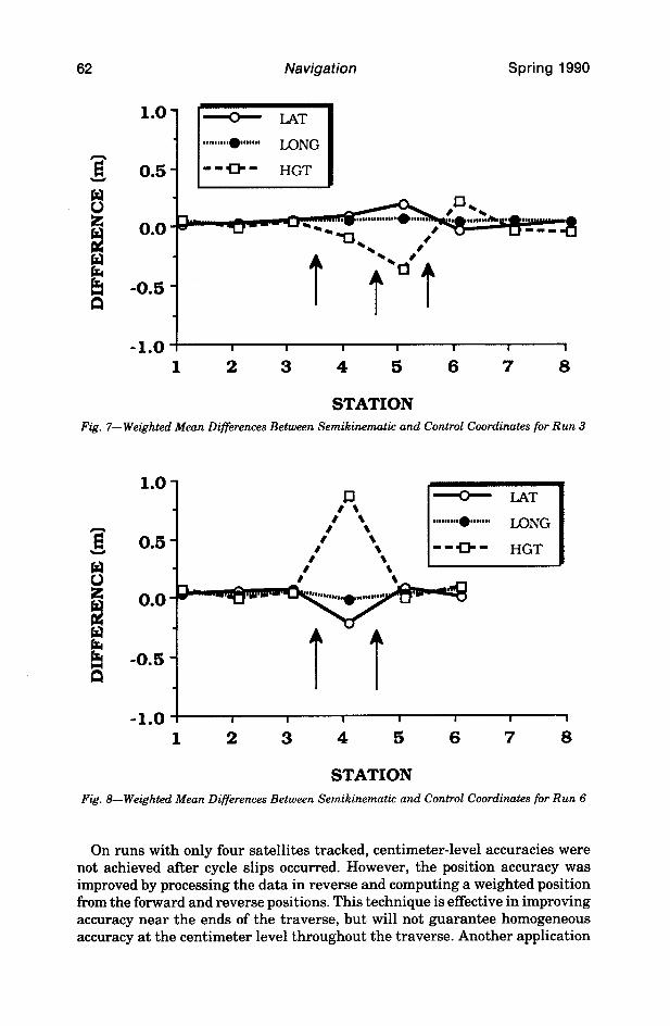
The weighted means of Runs 3 and 6 were computed from the forward- and reverse-processed positions. A weighted mean value at a control point was computed as follows (using height as an example):

(5)

where hM is the weighted mean height, hF is the height from forward processing, ai is the height variance from forward processing, h, is the height from reverse processing, and ai is the height variance from reverse processing.

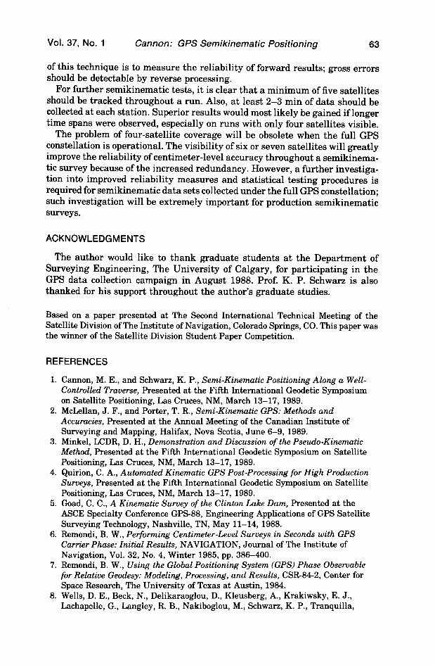
Weighted mean results are shown in Figures 7 and 8. They are much better than either the forward or reverse runs in the sense that centimeter-level accuracy is achieved at most stations. As seen in the figures, the accuracy of stations in the middle of the runs is generally not improved since the effect of the cycle slips could not be reduced.

CONCLUSIONS

The effectiveness of the two-step approach for semikinematic processing has been demonstrated using a well-controlled traverse. The approach uses a batch least-squares adjustment at static stations, as well as a Kalman filter to process pure kinematic data between static points. Accuracies of a few centimeters have been achieved on runs with five-satellite visibility, even in the presence of numerous cycle slips.

Navigation Spring 1990

0.0 -

-0.5 -

-1.0 : I I I I I I 1

1 2 3 4 5 6 7 8

STATION Fig. ‘I-Weighted Mean Differences Between Semikinematic and Control Coordinates for Run 3

8 \

0.0 - “em.,,,,, e---

-0.5 -

M

1 2 3 4 5 6 7 8

STATION

Fig. 8-Weighted Mean Differences Between Semikinematic and Control Coordinates for Run 6

On runs with only four satellites tracked, centimeter-level accuracies were not achieved after cycle slips occurred. However, the position accuracy was improved by processing the data in reverse and computing a weighted position from the forward and reverse positions. This technique is effective in improving accuracy near the ends of the traverse, but will not guarantee homogeneous accuracy at the centimeter level throughout the traverse. Another application


of this technique is to measure the reliability of forward results; gross errors should be detectable by reverse processing.

For further semikinematic tests, it is clear that a minimum of five satellites should be tracked throughout a run. Also, at least 2-3 min of data should be collected at each station. Superior results would most likely be gained if longer time spans were observed, especially on runs with only four satellites visible.

The problem of four-satellite coverage will be obsolete when the full GPS constellation is operational. The visibility of six or seven satellites will greatly improve the reliability of centimeter-level accuracy throughout a semikinematic survey because of the increased redundancy. However, a further investigation into improved reliability measures and statistical testing procedures is required for semikinematic data sets collected under the full GPS constellation; such investigation will be extremely important for production semikinematic surveys.

ACKNOWLEDGMENTS

The author would like to thank graduate students at the Department of Surveying Engineering, The University of Calgary, for participating in the GPS data collection campaign in August 1988. Prof. K. P. Schwarz is also thanked for his support throughout the author’s graduate studies.

Based on a paper presented at The Second International Technical Meeting of the Satellite Division of The Institute of Navigation, Colorado Springs, CO. This paper was the winner of the Satellite Division Student Paper Competition.

REFERENCES

1.

2.

3.

4.

5.

6.

7.

8.

Cannon, M. E., and Schwarz, K. P., Semi-Kinematic Positioning Along a Well- Controlled Traverse, Presented at the Fifth International Geodetic Symposium on Satellite Positioning, Las Cruces, NM, March 13-17, 1989. McLellan, J. F., and Porter, T. R., Semi-Kinematic GPS: Methods and Accuracies, Presented at the Annual Meeting of the Canadian Institute of Surveying and Mapping, Halifax, Nova Scotia, June 6-9, 1989. Minkel, LCDR, D. H., Demonstration and Discussion of the Pseudo-Kinematic Method, Presented at the Fifth International Geodetic Symposium on Satellite Positioning, Las Cruces, NM, March 13-17, 1989. Quirion, C. A., Automated Kinematic GPS Post-Processing for High Production Surveys, Presented at the Fifth International Geodetic Symposium on Satellite Positioning, Las Cruces, NM, March 13-17, 1989. Goad, C. C., A Kinematic Survey of the Clinton Lake Dam, Presented at the ASCE Specialty Conference GPS-88, Engineering Applications of GPS Satellite Surveying Technology, Nashville, TN, May 11-14, 1988. Remondi, B. W., Performing Centimeter-Level Surveys in Seconds with GPS Carrier Phase: Initial Results, NAVIGATION, Journal of The Institute of Navigation, Vol. 32, No. 4, Winter 1985, pp. 386-400. Remondi, B. W., Using the Global Positioning System (GPS) Phase Observable for Relative Geodesy: Modeling, Processing, and Results, CSR-84-2, Center for Space Research, The University of Texas at Austin, 1984. Wells, D. E., Beck, N., Delikaraoglou, D., Kleusberg, A., Krakiwsky, E. J., Lachapelle, G., Langley, R. B., Nakiboglou, M., Schwarz, K. P., Tranquilla,


J. M., and VaniEek, P., Guide to GPS Positioning, Canadian GPS Associates, Fredericton, New Brunswick, 1986.

9. Hofmann-Wellenhof, B., and Remondi, B. W., The Antenna Exchange: One Aspect of High Precision GPS Kinematic Survey, Presented at the International GPS-Workshop, Darmstadt, Federal Republic of Germany, April 10-13, 1988.

10 &lb, A., ed., Applied Optimal Estimation, M.I.T. Press, Cambridge, MA, 1974.

High-Accuracy GPS Semikinematic Positioning: Modeling and ...

Documents

Transcript of High-Accuracy GPS Semikinematic Positioning: Modeling and ...