Hierarchical Hidden Markov Model

of High-Frequency Market Regimes using

Trade Price and Limit Order Book Information

by

Shaul Wisebourt

A thesis

presented to the University of Waterloo

in fulfillment of the

thesis requirement for the degree of

Master of Quantitative Finance

Waterloo, Ontario, Canada, 2011

© Shaul Wisebourt 2011

ii

Author’s Declaration

I hereby declare that I am the sole author of this thesis. This is a true copy of the

thesis, including any required final revisions, as accepted by my examiners.

I understand that my thesis may be made electronically available to the

public.

Shaul Wisebourt

iii

Abstract

Over the last fifty years financial markets have seen an enormous expansion and development both in size

and variety. An industry that was once small and secluded has transformed into an essential part of

today’s economy. Such changes should in part be attributed to substantial advances in computer

technology. The latest allowed for a transition from face-to-face trading on organized exchanges to a

distributed system of electronic markets with new mechanisms serving the purposes of efficiency,

transparency and liquidity. In majority of cases this new trading system is driven by a double auction

market mechanism, in which market participants submit buy and sell orders, aiming to strike a balance

between certainty of execution and attractiveness of trade price. Generally, information about outstanding

buy and sell orders is made available to market participants in the form of a limit order book. It has been

suggested by multiple prior research that limit order books contain information that could be used to

derive market sentiment and predict future price movement.

In the current study we have presented ideas behind double auction market mechanism and have

attempted to model run and reversal market regimes using a simple and intuitive Hierarchical Hidden

Markov Model. We have proposed a statistical measure of the limit order book imbalance and have used

it to build observation (feature) vector for our model. We have built Limit Order Book analyzer – the

software tool that has become essential for data cleaning and validation, as well as extraction of feature

vector components from the data. We have used the model on high frequency tick-by-tick trade and limit

order book data from the Toronto Stock Exchange. We have performed the analysis of computational

results; for this purpose we have used a sample of annualized returns of stocks which comprised the

TSX60 index at the time of data collection; we have performed the comparative analysis of our results

with a simple daily buy & hold trading strategy as well as results of the trade price and volume model

presented in the prior research.

iv

Acknowledgements

Work on this thesis would not be possible without support of my research advisor, Professor Yuying Li.

At every stage of this long process she was there to provide guidance; she inspired me to try out new

things and taught to stay focused. She helped make this thesis a great learning and research experience.

I am indebted to Aditya Tayal for insightful conversations about financial markets and his helpful

suggestions on modeling.

I am thankful to my family for their patience, encouragement and continuing moral support.

v

Table of Contents

Author’s Declaration ................................................................................................................................. ii

Abstract .................................................................................................................................................... iii

Acknowledgements .................................................................................................................................. iv

Table of Contents ...................................................................................................................................... v

List of Figures ......................................................................................................................................... vii

List of Tables ........................................................................................................................................... ix

Introduction ............................................................................................................................................... 1

Academic Contribution ......................................................................................................................... 6

Thesis Outline ....................................................................................................................................... 7

Chapter 2 Market Microstructure: Order Types, Time and Sales, Limit Order Book .............................. 8

2.1 Orders and Order Types .................................................................................................................. 8

2.2 Trades ............................................................................................................................................ 10

2.3 Double Auction Market Mechanism – Limit Order Books........................................................... 12

Chapter 3 Statistical Modeling of Financial Time Series: Hidden Markov Models ............................... 16

3.1 Overview ....................................................................................................................................... 16

3.2 Hidden Markov Models ................................................................................................................ 18

3.3 Hierarchical HMMs ...................................................................................................................... 27

3.4 Dynamic Bayesian Networks ........................................................................................................ 28

vi

Chapter 4 Trade Price and Limit Order Book -based Model ....................................................... 30

4.1 Volume-Weighted Average Price ( ) .................................................................................. 30

4.2 Order Book Imbalance .................................................................................................................. 34

4.3 Zigzag Aggregation of Time Series .............................................................................................. 36

4.4 Model Specification and Feature Vector Extraction ..................................................................... 39

Chapter 5 Computational Results ........................................................................................................... 49

5.1 Limit Order Book Analyzer .......................................................................................................... 49

5.2 Data Set ......................................................................................................................................... 52

5.3 Learning the Model from the Data ................................................................................................ 53

5.4 Out-of-Sample Inference ............................................................................................................... 57

Conclusions ............................................................................................................................................. 69

References ............................................................................................................................................... 72

vii

List of Figures

Figure 1: Time and Sales of the TSX:RIM stock on May 1st 2007 at noon. .............................................. 11

Figure 2: Bid and ask stacks of a limit order book; the TSX:RIM stock on May 1st 2007 at noon. .......... 15

Figure 3: An example of a simplest Markov model – a Markov chain. ...................................................... 19

Figure 4: An example of a hidden Markov model. ..................................................................................... 22

Figure 5: An illustration of a four-level HHMM ........................................................................................ 28

Figure 6: State of the TSX:RIM limit order book at 11:59 AM on May 1, 2007. Outlined in blue crossed

markers are the bid and the ask prices and cumulative volume sizes calculated at 10-row depth. 32

Figure 7: State of the TSX:RIM limit order book at 12:00 PM on May 1, 2007. Outlined in red dotted

markers are the bid and the ask prices and cumulative volume sizes calculated at 10-row depth. 32

Figure 8: Time and Sales show the trade in 100 shares of TSX:RIM at $147.68. ...................................... 33

Figure 9: Time series of the May 1, 2007 TSX:RIM trade price, bid and ask s calculated at the 10-

row depth. Blue crossed markers and red dotted markers correspond to data points in Figures 6, 7. Plain

green marker denotes the trade in Figure 8. ................................................................................................ 33

Figure 10: Balanced Limit Order Book: and

are equally distanced from the current

market price. ............................................................................................................................................... 35

Figure 11: Imbalanced Limit Order Book: a) market price is skewed towards and therefore

faces resistance from highly dense at lowest ask prices sell side of the order book – we expect market

price to go down; b) market price is skewed towards and therefore faces support from highly

dense at highest bid prices buy side of the order book – we expect market price to go up ........................ 35

viii

Figure 12: Time series of the May 1, 2007 TSX:RIM trade price from Figure 9. The blue square markers

correspond to the plateau and the valley trades; the red circle markers correspond to the end-of-zigzag

trades; the green crossed circle markers correspond to the zigzag internal trades. ..................................... 37

Figure 13: Time series of the May 1, 2007 TSX:RIM trade price. The solid red lines correspond to the

trends identified at high retracement levels; the double green line corresponds to trends identified with

lower retracement levels. ............................................................................................................................ 40

Figure 14: A schematic representation of a graphical model that incorporates our knowledge about the

existence of runs and reversals as well as short-lived micro trends within those runs and reversals. ........ 41

Figure 15: The Hierarchical Hidden Markov model of the price and limit order book. ............................. 43

Figure 16: A snapshot of the Limit Order Book Analyzer tool. ................................................................. 51

Figure 17: Distributions of zigzags with the local maxima and minima derived from the TSX60 data using

the price trend and limit order book feature. ............................................................................................... 54

Figure 18: Distributions of zigzags with the local maxima and minima derived from the TSX60 data using

the price trend and volume feature. ............................................................................................................. 55

Figure 19: Distributions of zigzags conditional on the hidden state, aggregated over a 5-day rolling

window – the price trend and limit order book feature. .............................................................................. 56

Figure 20: Distributions of zigzags conditional on the hidden state, aggregated over a 5-day rolling

window – the price trend and volume feature. ............................................................................................ 57

Figure 21: The value of $1 invested in the four quartiles of different liquidity for the month of May 2007

.................................................................................................................................................................... 60

Figure 22: The value of $1 invested in the TSX60 Index for the month of May 2007. .............................. 61

Figure 23: Annualized returns data from the price and limit order book model and the fitted distributions

in run and reversal regimes. ........................................................................................................................ 64

Figure 24: (a) a -plot of the annualized returns in the run regime vs. quantiles of the Standard Normal

distribution; (b) a -plot of the annualized returns in the reversal regime vs. the quantiles of the

Standard Normal distribution. ..................................................................................................................... 65

Figure 25: The annualized returns data from the price and volume model and the fitted distributions in the

run and reversal regimes. ............................................................................................................................ 66

ix

List of Tables

Table 1: The annualized return of the S&P 500 Total Return Index and ...................................................... 3

Table 2: Percentage of runs with no change in price for 0, 1, 2, 3 and more than 3 trades. ....................... 38

Table 3: The trade price and Imbalance feature space (from Tayal [38]). ..................................... 48

Table 4: The quartile groupings of the TSX60 tickers by the average daily volume ................................. 59

Table 5: Descriptive statistics of the annualized trade returns. ................................................................... 61

Table 6: The maximum daily draw-down of the B&H and LOB strategies. .............................................. 62

Table 7: Descriptive statistics of the regime-conditional annualized trade returns .................................... 62

Table 8: Descriptive statistics of the conditional annualized trade returns: ................................................ 64

Table 9: The results of a two-sample t-test conducted at 5% significance level on annualized returns data

from price and LOB and price and volume models. ................................................................................... 67

Table 10: The results of a paired -test conducted at 5% significance level on annualized returns data from

price and LOB and price and volume models. ............................................................................................ 68

1

Introduction

One question that every investor asks before committing capital to an investment opportunity is about its

expected return. In most cases the answer depends on the nature of the undertaking, and in particular on

the level of risk involved. In general, investors can expect to be compensated more when they run higher

risks of not seeing back the originally invested money. This principle seems to be intuitively plausible,

however the question of whether the rule always holds true, or if there exist investment opportunities with

similar risk profile, but different levels of return, still remains to be answered. If such opportunities

existed simultaneously and information about their existence was readily available, a typical investor

would choose the one with a higher level of return1. Furthermore, a combination of such opportunities

could yield risk-free return.

Hence the most natural answer is that such opportunities do not exist in practice. Indeed, if they

existed, every investor would be interested in higher return opportunity, and demand for it would greatly

outweigh supply, which in turn would bring the level of return down, in line with other opportunities.

This would hold especially true in transparent markets where all investors are well-informed about

existing opportunities, and asset prices consistently reflect the level of risk associated with those assets. In

such markets any new information would disseminate among market participants in an efficient manner

and the prices would adjust very quickly, therefore leaving no space for the systematic risk-free profiting.

1 Similarly if two opportunities with the same level of expected return by different risk profiles existed, a typical

investor would be inclined to choose the one with the lower risk.

2

In the context of financial markets, this idea was put into the basis of the Random Walk

Hypothesis, popularized by Samuelson [32], and later on further developed and formalized into the

Efficient Market Hypothesis (EMH) by Fama [11]. The EMH suggests that based on the level of

informational awareness any financial market can be classified as efficient in a weak, semi-strong, or

strong form. In a market with the weak form of efficiency, future prices cannot be predicted from

historical prices, therefore rendering technical analysis useless; there are no patterns in historical time

series that could provide any clues into the future market prices; in the absence of changes in fundamental

information, price movements are random, and therefore an investor shouldn’t expect to be able to make

risk-adjusted returns higher than those offered by the general market in a consistent manner. The semi-

strong form further denies fundamental analysis of any predictive power due to the fact that any new

information spreads out in the market rapidly and therefore trading on such information cannot bring any

excess returns. The strong form of hypothesis extends information awareness beyond publicly available

information; public availability of private (insider) information ensure that participants in the market with

the strong form of efficiency cannot consistently earn excess returns.

Theory behind EMH has seen some extensive support in the empirical evidence and it has been

well accepted by many practitioners, including some heavy-weight market players like mutual fund

managers. Such managers run beta programs and, depending on fund’s prospectus, get exposure to either

a specific industry or market as a whole by investing in industry- or market-wide indices, respectively.

They would not employ any winner-picking strategies based on fundamental or technical analysis, but

would rather expect to make returns consistent with the level of risk taken. If investors require higher

returns, those can be obtained by borrowing additional funds on margin and leveraging the initial

investment. However, in this case the risk increases along with the expected return, therefore keeping

risk-return profile unchanged.

Despite popularity of EMH during 1970s, some evidence was found against it. In particular, stock

markets appeared to have tendency to trend over periods of time [31]. Mean-reverting properties of price

processes were revealed in analysis of some correlated time series. Quite opposite to the EMH, such

market inefficiencies persisted for prolonged periods of time, which yielded excess returns for some

market participants. Starting in 1980s, a whole new type of market participants, the hedge funds,

emerged. Unlike mutual funds, hedge funds have concentrated their efforts on alpha programs, looking

for different ways to exploit market inefficiencies in a systematic way. By the very nature of their

activities, hedge fund managers rejected EMH, and concentrated on winner-picking, trend following,

mean-reverting and many other strategies with the sole purpose of earning excess returns from investment

activities. Initially, these efforts have seen a fair amount of skepticism: a number of hedge funds have

3

failed, and success of others has been attributed to pure luck and co-incidence. However, as time passed,

the hedge fund industry has found its own leaders. The two most prominent ones are the Quantum

Endowment Fund established in 1972 by a renowned economist George Soros, and the Renaissance

Technology Medallion Fund, which was started back in 1982 by a brilliant mathematician Jim Simons.

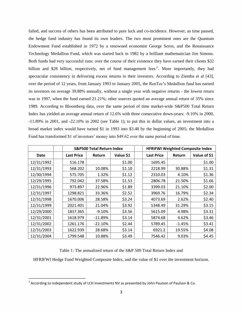
Both funds had very successful runs: over the course of their existence they have earned their clients $32

billion and $28 billion, respectively, net of fund management fees2. More importantly, they had

spectacular consistency in delivering excess returns to their investors. According to Ziemba et al [43],

over the period of 12 years, from January 1993 to January 2005, the RenTec’s Medallion fund has earned

its investors on average 39.88% annually, without a single year with negative returns - the lowest return

was in 1997, when the fund earned 21.21%; other sources quoted an average annual return of 35% since

1989. According to Bloomberg data, over the same period of time market-wide S&P500 Total Return

Index has yielded an average annual return of 12.6% with three consecutive down-years: -9.10% in 2000,

-11.89% in 2001, and -22.10% in 2002 (see Table 1); to put this in dollar values, an investment into a

broad market index would have turned $1 in 1993 into $3.48 by the beginning of 2005; the Medallion

Fund has transformed $1 of investors’ money into $49.62 over the same period of time.

S&P500 Total Return Index HFRIFWI Weighted Composite Index

Date Last Price Return Value $1 Last Price Return Value of $1

12/31/1992 516.178 $1.00 1695.45 $1.00

12/31/1993 568.202 10.08% $1.10 2218.99 30.88% $1.31

12/30/1994 575.705 1.32% $1.12 2310.03 4.10% $1.36

12/29/1995 792.042 37.58% $1.53 2806.78 21.50% $1.66

12/31/1996 973.897 22.96% $1.89 3399.03 21.10% $2.00

12/31/1997 1298.821 33.36% $2.52 3969.76 16.79% $2.34

12/31/1998 1670.006 28.58% $3.24 4073.69 2.62% $2.40

12/31/1999 2021.401 21.04% $3.92 5348.49 31.29% $3.15

12/29/2000 1837.365 -9.10% $3.56 5615.09 4.98% $3.31

12/31/2001 1618.979 -11.89% $3.14 5874.68 4.62% $3.46

12/31/2002 1261.176 -22.10% $2.44 5789.45 -1.45% $3.41

12/31/2003 1622.939 28.68% $3.14 6921.2 19.55% $4.08

12/31/2004 1799.548 10.88% $3.49 7546.42 9.03% $4.45

Table 1: The annualized return of the S&P 500 Total Return Index and

HFRIFWI Hedge Fund Weighted Composite Index, and the value of $1 over the investment horizon.

2 According to independent study of LCH Investments NV as presented by John Paulson of Paulson & Co.

4

The returns of the hedge fund industry as a whole over the same period of time are less

impressive than those of the Medallion Fund. However, as it can be seen from Table 1, the annualized

compounded returns are still higher than those of the S&P500 Total Return Index, and the investment

risk, as measured by the standard deviation of returns and maximum draw downs, is considerably smaller.

It is hard to ignore such spectacular results and blindly follow the EMH, even for academia. A

number of statistical tools have been found to be applicable to forecasting of financial time series. Simple

linear factor models as well as autoregressive (AR), moving average (MA), autoregressive moving

average (ARMA) models were historically first. Non-linear models have been found to be successful in

some forecasting applications [25]. Over the course of 1990s, in part due to significant advances in

computer technology, modeling focus has shifted towards data driven models, which involved model

learning over vast sets of data; to name a few, we mention genetic algorithms, reinforcement learning,

artificial neural networks and hidden Markov models. Due to their flexibility and high adaptability to

various kinds of problems hidden Markov models (HMM) became one of the most popular modeling

approaches.

Among recent studies of financial markets which employ HMMs is the work of Tayal [38]. The

author has designed a high-frequency regime-switching hierarchical hidden Markov model of trade price

and volume. His study has been inspired by technical analysis: the main concept behind the model is that

of interaction between the price of a security and the traded volume in different market regimes. Novelty

of the approach comes from the underlying probabilistic framework – the dynamic Bayesian network

(DBN) - employed for the technical pattern learning and inference purposes. The DBNs have seen prior

successful applications in the computationally intensive fields of speech recognition, bio-sequencing,

visual interpretation, etc. The regime-switching model of Tayal adds to this success – it was able to

identify run and reversal market regimes in TSX60 price and volume data in a statistically significant

way. The study presented results of statistical tests which suggest that the model was able to capture

unique trade return distributions conditional on market regimes. These results presented strong evidence

in support of the information content being available in price and volume intraday high-frequency data,

further undermining the EMH.

Sophisticated computer technology has also affected the way financial markets operate, and has

contributed to the transition from face-to-face trading on organized exchanges to a distributed system of

electronic markets with new mechanisms of achieving better efficiency, transparency and liquidity. In

majority of cases this new trading system is driven by a double auction market mechanism, in which

market participants submit buy and sell orders, aiming to strike a balance between the certainty of

execution and the attractiveness of the trade price. Generally, the information about outstanding buy and

5

sell orders is made available to market participants in the form of a limit order book. Such transparency of

inherently rich market microstructure data spurred great interest to modeling of the limit order book, and

this has become an intriguing topic both in academia and among practitioners [20]. Several aspects are of

particular interest: the distribution of the price and volume in limit order books, the effects of the limit

order book’s density on bid-ask spread, the trade price development.

It has been suggested by the multiple prior research that limit order books contain information

that could be used to predict future price movements3. Limit order books have been studied from different

angles. Cao et al [4] have used limit order information from the Australian Stock Exchange to examine

the effects of limit order books on investors’ order placement strategies; they found that top of the order

book (up to ten top-level limit orders) has significant effect on order submissions, cancellations and

amendments. Slanina [36] has developed a limit order driven market model and studied forces behind

evolution of limit order books. Cont et al [6] have used high-frequency observations to study dynamics of

limit order books and proposed a stylized continuous-time stochastic model; among other applications,

their model can be used to calculate probabilities of certain events of interest, such as increase in mid-

price, execution of an order at the bid before changes in the ask quotes, execution of buy and sell order at

the best quotes before the price moves, all of the above events conditional on the state of the limit order

book; authors have found that their model has adequately captured behavior of the limit order book and

generated useful short-term predictions, sufficient to build a successful simple trading strategy. Some

effort was directed towards modeling of limit order volume and price distributions. Zovko et al [44]

discovered that relative limit prices follow power law with significant price clustering. Considerable

effort to study behavior and predictive power of limit order books was undertaken within the framework

of the Penn-Lehman automated trading project [21]. The centerpiece of the project, the Penn Exchange

Simulator, was developed based on limit order data from the Island ECN. The majority of trading

strategies employed by the project participants were based on limit order book models. The basic static

order book imbalance model offered to participants was further developed to incorporate online parameter

learning algorithms and real-time measures of volatility.

In the current study we present a simple and intuitive Hierarchical Hidden Markov Model

(HHMM) of high-frequency market run and reversal regimes. We describe double auction market

mechanism and propose a statistical measure of the limit order book imbalance. Our objective is to extract

valuable information from the vast limit order book data. The resulting measure, along with trade price

trend indicators, is put together to build a feature vector, which is used by the HHMM framework to

derive optimal (in probabilistic sense) predictions of the future state of a financial market. The ultimate

3 According to internal sources, the earlier mentioned RenTec’s Medallion Fund made use of the Nasdaq and New

York Stock Exchange limit order books in its trading strategies [3].

6

goal of the study is to investigate whether there is any evidence in the trade price and limit order book

data against the EMH.

Academic Contribution

Work presented in this thesis is of a quantitative finance nature and is based on a symbiosis of

mathematics and computer science.

At the early stages of research significant effort has been dedicated to development of a software

application – Limit Order Book (LOB) Analyzer (Figure 16), which has greatly helped navigating the

tick-by-tick trade and limit order book data. Besides data cleaning and identification of the problems

encountered in data, LOB Analyzer has been essential in calculation of the LOB-based component of the

feature vector. As shown in Chapter 4, it is fairly easy to calculate price direction and magnitude

components of the feature vector directly from the trades data, as such calculations are dependent only on

time, and the trades data is chronologically ordered. However, the LOB-based component of the feature

vector required calculations on the order book stacks, which are ordered based on both the limit price and

the time of order arrival. The task would be daunting to complete without the LOB Analyzer tool.

In addition, we have proposed a measure of imbalance of the limit order book and, based on this

measure, we have built an HHMM of the high-frequency market regimes driven by the trade price and the

limit order book data.

Furthermore, we have performed analysis of the computational results; for this purpose we have

used a sample of annualized returns of stocks which comprised TSX60 index at the time of data

collection; we have performed comparative analysis of our results with a simple daily buy & hold trading

strategy.

Finally, we have assessed model’s ability to distinguish the run and reversal market regimes out-

of-sample. We have validated results of the price and volume model presented in Tayal [38] and

performed the comparative analysis of our results with results of the price and volume model.

7

Thesis Outline

In Chapter 2 we provide necessary background on market microstructure, and describe double auction

mechanism. Chapter 3 provides a short summary of classical approach to modeling of financial time

series, and further describes theory behind statistical models used in our study: Markov processes and

Hidden Markov models. Special attention is paid to learning and inference stages of the modeling

process. In Chapter 4 we discuss volume-weighted average price and introduce the order book imbalance

feature; we describe intuition behind our model and briefly discuss mechanics of time series processing

and extraction of the feature vector. In Chapter 5 we describe the Limit Order Book Analyzer tool and the

Toronto Stock Exchange high-frequency data set used in our experimental analysis. The same chapter is

used to report computational results. Finally, we summarize our conclusions, and provide some insights

into future research.

8

Chapter 2

Market Microstructure: Order Types, Time and Sales,

Limit Order Book

In this chapter we review concepts which are essential to the understanding of any trading model in the

context of a modern financial market. In particular, we discuss different types of orders available to

market participants and talk about mechanics of double auction markets and limit order books. These are

often collectively referred to as market microstructure [21].

2.1 Orders and Order Types

Before we get to describe the double auction market mechanism, we need to introduce the trading

order concept, and discuss different order types. In the context of the current study, we define an order in

a financial market as an instruction from a trader to a public exchange, either directly or through a broker,

to buy or sell a security4.

4 A general definition of an order would include over-the-counter orders submitted via private venues (proprietary

trading systems) from a customer, usually a large financial institution, to a broker or a dealer. These are of no interest to us, as they are isolated from public markets and therefore do not contribute to supply and demand on exchanges.

9

We should clearly distinguish order types which are universally supported by the public

exchanges from custom order types supported by specific brokerages. Good examples of standard order

types are market and limit orders. Terms and conditions for these order types are clearly defined by the

exchange and they are universal for all participants. These are the only types of orders that can be

submitted to the exchange by its participants. Such orders fit well into the double auction mechanism of

any public exchange5. These orders are tracked by the exchange and therefore order-flow information is

available through the exchange for a data subscription fee. Public availability of data makes such orders

good candidates for the academic research.

In the current study we utilize only publicly available exchange-level information. Hence,

classification of order types given below is primarily based on price level constraints, which have to be

met for the execution to take place. We also introduce a classification based on the time period during

which the order is valid, and describe special order types which are the major source of dark liquidity in

the markets. We follow the standard definitions proposed by the U.S. Securities and Exchange

Commission [34].

Any order can be submitted as either a day order, or a good-till-cancelled (GTC) order. Day order

is the default type of order used by brokerages. Such orders are good for one trading day in which they

are submitted. Orders that have been placed but have not been executed during regular trading hours will

not automatically carry over into the after-hours trading session or the next trading day - they will be

cancelled by the exchange. Unlike the day orders, GTC orders last until they have been successfully filled

or cancelled. A designated cancelling order is required to remove the original GTC order. Since the

lifespan of day orders is fairly short, they are usually placed closer to the prevailing market price, and

therefore such orders constitute the majority of the publicly traded daily volume. GTC orders on the other

hand are often used by investors to set limit prices which are far away from the current market price,

leaving them somewhat out of the “hot” market action.

From the perspective of price level constraints, we distinguish market and limit orders. A market

order is an order to buy or sell a security at the current market price. A market order, submitted by a

brokerage to the exchange, gets executed immediately, provided that market liquidity is in place - there

are willing buyers and sellers to meet the volume requested in the order. There are no constraints set on

the execution price level for a market order – it gets filled at the current market price. Such orders can be

met by opposite side market orders. When no matching opposite side market order is available, the market

order is filled at the best bid (for sell market orders) or at the best ask (for buy market orders), whatever

5 The double auction mechanism is defined later in this chapter.

10

those price levels are. Therefore, market orders favor the certainty of execution over the price level of

execution. A market order, compared to a limit order, has an increased likelihood of being filled, but there

is no guarantee over the price of execution – it can be far away from the bid-ask spread at the time when

the order is submitted. This holds especially true for volatile markets, when abrupt market movements are

likely.

Limit order is there to address price uncertainty of a market order. A buy limit order is an order to

buy a security at a price no more than the specified limit price. Such order can be filled at a price which is

lower than the limit price, and therefore more beneficial to the buyer. On the other hand, a sell limit order

is an order to sell at price no less than the specified limit price. Similarly to buy limit orders, sell limit

orders can be filled to a greater benefit for the seller, but in this case the execution price has to be higher

than the limit price. A trader submitting a limit order has complete control over the price level at which

the order will be executed. However, it is uncertain whether such an order will be filled at all. It might

well be that market participants would not be willing to transact at the limit price. Therefore, there is no

guarantee that the limit order will be filled. Unlike market orders, limit orders favor certainty of price

over uncertainty of execution. A limit order that does not get filled is placed onto limit order book (LOB),

according to the rules described in the next section. It remains on the book until either market conditions

change and the order gets filled, or until it is cancelled/expired.

2.2 Trades

Every time a pair of orders of any type described in the previous section is matched by price and

volume a trade takes place. All trades are recorded on Time & Sales (T&S), which is a list maintained by

an exchange. Each trade-record on T&S will contain price and volume information, as well as time when

the trade occurred. Often bid-ask spreads and their supporting volumes are recorded as well.

All the examples and corresponding figures in the following discussion were obtained using the

Limit Order Book Analyzer – a tool that we built for the purposes of data cleaning, data validation,

feature vector extraction and analysis. We provide a detailed description of the LOB Analyzer in Chapter

5.

We shall look at the following example in order to get a better understanding of T&S. Suppose

we are interested in shares of Research in Motion, listed on the Toronto Stock Exchange under the symbol

RIM. State of the market for this ticker on May 1st 2007 around noon time is illustrated in Figure 1. In our

example, last trade, #1578, has happened at 11:59:58 AM for 100 shares of RIM and was transacted at

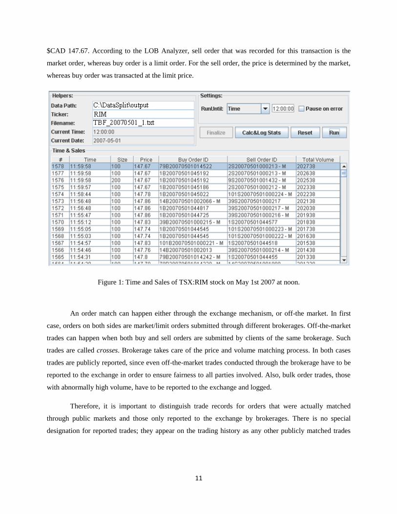
11

$CAD 147.67. According to the LOB Analyzer, sell order that was recorded for this transaction is the

market order, whereas buy order is a limit order. For the sell order, the price is determined by the market,

whereas buy order was transacted at the limit price.

Figure 1: Time and Sales of TSX:RIM stock on May 1st 2007 at noon.

An order match can happen either through the exchange mechanism, or off-the market. In first

case, orders on both sides are market/limit orders submitted through different brokerages. Off-the-market

trades can happen when both buy and sell orders are submitted by clients of the same brokerage. Such

trades are called crosses. Brokerage takes care of the price and volume matching process. In both cases

trades are publicly reported, since even off-the-market trades conducted through the brokerage have to be

reported to the exchange in order to ensure fairness to all parties involved. Also, bulk order trades, those

with abnormally high volume, have to be reported to the exchange and logged.

Therefore, it is important to distinguish trade records for orders that were actually matched

through public markets and those only reported to the exchange by brokerages. There is no special

designation for reported trades; they appear on the trading history as any other publicly matched trades

12

would6. For example, a bulk order trade of 500-times average order’s volume gets reported to the

exchange and is recorded on the T&S. However, market price of the security is not affected by such

order. In after-hours trading, conditional orders, like -guaranteed7, can cause a jump in the

recorded price of the trade with no visible sign of change in the LOB. For these reasons reported trades

have to be filtered out. Such cleaning was performed in our study on the raw dataset and the rules that

have been applied are discussed in Chapter 5.

2.3 Double Auction Market Mechanism – Limit Order Books

Organizational structure of a classic pit-based exchange did not encourage (neither it could handle) direct

access to trading for the majority of market participants. For liquidity purposes such environment was

heavily dependent on market makers, where a market maker is a participant of an organized market, who

is prepared to quote both bid and ask prices on a given financial instrument. Some exchanges, like the

New York Stock Exchange (NYSE) and American Stock Exchange (AMEX), even had official

designated market makers, also known as specialists, who traded market in a particular set of securities.

Under such organizational structure, market makers became the primary source for liquidity on exchange.

Over the last fifty years the landscape of financial markets has dramatically changed. Being early

adopters of technology, exchanges around the globe have replaced pit trading with electronic trading

platforms to a great extent. Some regulated exchanges, like NASDAQ, became completely electronic,

screen-based trading markets. As of today all orders submitted on NASDAQ are routed via electronic

order routing system, and order matching is performed by NASDAQ’s computer system. Electronic

trading has received even a larger boost with the advent of Electronic Communication Networks (ECNs),

which were officially authorized by the US SEC in 1998, with trading going on virtually around the

clock. There are multiple drivers behind these changes, starting with the mere convenience of automating

procedures that used to be performed manually and moving on to a greater market and price transparency,

faster order processing and, most importantly, increased liquidity.

Most recent development in electronic markets is the direct access to trading resources by a large

number of market participants. It has resulted in increased liquidity and allowed exchanges to shift

6 This is the case with the TSX streamed data used in our analysis; it also holds true for most publicly available data.

More advanced, professional data systems, like Bloomberg, provide special trade codes with each trade, so that traders (or trading algorithms) can easily distinguish between publicly executed and reported trades. 7 A -guaranteed order is a conditional order offered by some brokerages; it guarantees time-constrained

volume-weighted execution price.

13

operation to order-driven basis. There are still market makers in such markets. However their role in

providing liquidity has greatly diminished. Incoming buy and sell orders are matched by the exchange’s

electronic system. Matching orders are brought together and a trade is executed. Limit orders that cannot

be matched by the system, end up in buy and sell waiting queues, collectively known as the limit order

book (LOB), or the market depth.

The LOB is a collection of buy and sell limit orders arranged into bid and ask stacks,

respectively. Such arrangement is based primarily on the limit price and, secondarily, on the order arrival

time. On both sides of the book only limit orders are stored. Rules, which apply to order book

organization, ensure that the most competitive orders, those with the limit prices closer to the bid-ask, are

favored. For the bid side of the LOB, orders with the higher price are positioned closer to the top of the

bid stack, whereas for the ask side, orders with the lower price are placed closer to the top of the ask

stack. Orders that appear on the same side of the order book and have the same price are positioned on the

stack based on time of arrival of such orders, with those having an earlier timestamp being placed closer

to the top of the book. On the bid side, prices of all orders are less than those on the ask side8. If this were

not the case, it would imply that buyers are willing to pay price that is higher than the price at which

sellers are willing to sell. This would automatically result in trades taking place until there are no more

orders on the LOB with buy order limit prices higher than sell-order limit prices. The two top-most orders

on the LOB (one from bid side and another from ask side) form the market’s bid-ask spread.

There are several ways in which orders can be removed from the LOB. Since market conditions

are constantly changing, many of the limit orders are short-lived and get submitted to the exchange as day

orders. They automatically expire by the end of trading day and get removed from the LOB9. On the other

hand, good-till-cancelled orders are removed from LOB only after a special cancellation order is

submitted. Any limit order, which no longer satisfies the requirements of a trading strategy due to

changing market environment, can be explicitly cancelled as long as it has not been filled prior to the

submission of the cancellation order. Finally, a limit order gets removed from the LOB when it gets filled.

8 Strictly speaking, there are situations when bid and ask side of the limit order book overlap, but they are

concerned with very specific limit orders. These include AON (all-or-none) limit orders, for which the order does not get executed until there is an opposite side order with both matching price and matching volume. Large volume AON orders are rarely to be seen on the LOB since order initiators try to split the initial order into multiple orders of smaller size, or submit an iceberg order to avoid market impact. Therefore most often LOB overlaps occur with odd size lot orders, where size of the order is not a multiple of a hundred. These, however, do not make large volume impact and also get removed from the LOB quickly enough to ignore them when claiming that LOB stacks do not overlap. 9 Day orders can outlive the closing market bell, which is, for example, 4:00 pm EST on NASDAQ, and stay on the

LOB until 8:00 pm if they are submitted as “valid after-hours”; but even such orders do not survive from one trading session to another and get automatically removed from the LOB once after-hours trading is closed.

14

This can happen when an opposite side market order or a buy (sell) side limit order with limit price higher

(lower) than the limit price of the order in the LOB hits the market. In this case a trade gets recorded on

the T&S. If the available trade volume is greater or equal to the limit order volume, limit order gets

removed from the LOB. Partially filled limit order remains on the LOB in the original position (provided

no order with a better price arrives) until it’s either completely filled or cancelled for the remaining

volume. In cases when limit order on the LOB is matched with the incoming limit order, the price of the

order on the LOB is the one that gets recorded on the T&S as the execution price [20].

Continuing with the example of the RIM stock traded on May 1, 2007 at noon, the state of the

limit order book at this time is illustrated on Figure 2. Bid and ask stacks of the limit order book are

displayed on the Bid and Ask panes. The best bid price is $CAD 147.67, whereas the best ask price is

$CAD 147.75. Note that at this time the price of the last trade is identical to the best bid on the LOB. This

is a mere coincidence, and does not have to be the case in general. As a matter of fact, bid-ask bracket

often moves away from the price of last trade very quickly, especially in volatile markets. Again, the only

requirement is that bid prices are lower than ask prices, which is the case in this example. Buy limit

orders are inserted into the bid stack of the LOB based on their limit prices. The higher the price is the

closer the order gets placed to the top of the bid stack. Suppose a new buy order with the limit price of

$CAD 147.65 arrives next. It is then inserted on the bid side of the book at the fifth position, shifting

down existing buy orders with lower limit prices. On the opposite side, for sell limit orders, a lower limit

price puts the order closer to the top of the ask stack. If the next order to arrive is a sell order with the

limit price of $CAD 147.76, it is inserted at the second position on the ask side, therefore shifting all the

sell orders with a higher limit price by one position down.

As can be seen from the LOB snapshot, it is quite possible for orders with the same price on one

side of the book to co-exist. Multiple orders with the same price get placed onto the LOB stacks based on

their time of arrival, with those orders arriving earlier in the day being placed closer to the top of the

LOB. Application of this rule can be easily seen for orders which are further away from the current

market price. In particular, consider orders #33-42 submitted on the bid side of the LOB. For all orders

submitted at the limit price of $CAD 146.00, the ones submitted earlier in the day are placed closer to the

top of the bid stack. Similarly, sell orders #25-28 are all submitted at the price of $CAD 148.50; orders

higher on the ask stack have earlier timestamps.

Now, if a sell market order for 1,000 shares of RIM were to arrive, it would have completely

consumed buy limit orders #1 to #4 at $CAD 147.67 per share, and order #5 would be partially filled, 200

shares at $CAD 147.64. Orders #1 to #4 would be completely removed from the bid stack, and order #5

15

would move to the top of the stack with the remaining volume of 2,300 shares and the limit price of

$CAD 147.64. Similar logic holds for the arriving buy market order with respect to the ask stack of the

LOB.

Figure 2: Bid and ask stacks of a limit order book; the TSX:RIM stock on May 1st 2007 at noon.

The number of limit orders that appear on each side of the exchange-maintained LOB is

unlimited by the exchange (in the current example there are 143 buy limit orders and 244 sell limit

orders). However, many of these orders are significantly away from the current “market action”.

Therefore many brokerages maintain and publish a truncated version of the LOB, with the standard being

fifteen to twenty top orders on each side propagated to traders.

16

Chapter 3

Statistical Modeling of Financial Time Series:

Hidden Markov Models

In the current chapter we provide an overview of tools used for statistical modeling of financial time

series, focusing on models that are used in our study – the (Hierarchical) Hidden Markov Models and

Dynamic Bayesian networks.

3.1 Overview

Analysis of financial time series has a long history with a wide spectrum of statistical models used for the

purpose of forecasting10

.

Simple linear models such as autoregressive (AR), moving average (MA) and autoregressive

moving average (ARMA) were historically first. A time series is said to be linear if its model can be

defined as

10

For a comprehensive coverage of such statistical tools see [41].

17

where is the mean of , are weights defining dynamic structure of with , and is a

sequence of random variables with mean zero and a well-defined distribution – is a shock at time

[41]. Underlying these models is the assumption of linearity of data. Another standard assumption for

linear models is weak stationarity. Suppose that is a weak stationary time series; then the mean of

is constant, the covariance between and is also constant for integer , i.e. covariance is constant

for a given lag. In practice, most financial data is non-linear. This translates into dependency of residuals

in a linear model, which can be verified using nonparametric (Q-statistic of squared residuals, Bispectral,

etc.) or parametric (F, Thereshold) tests. Failure to pass such tests yields inadequacy of the linearity

assumption and therefore proves simple linear models unusable. Weak stationarity requires one to assume

a finite (of length ) historical window with recurrent pattern of behavior. Such fixed-length window

might be unknown and hard to identify, or too restrictive and simple to yield results useful for

applications such as prediction.

Non-linear models proved useful in overcoming deficiencies of simple linear models in analysis

of financial time series. A comparative example of modeling using linear (AR) model vs. non-linear

model (MCMC) is provided in [25]. In particular, changes in seasonally adjusted U.S. civilian

unemployment rate time series from 1948 to 1993 analyzed using AR model fail to pass linearity test,

whereas applying Markov switching model yields better forecasting results. A non-linear model of can

be written in terms of its conditional moments [41]. If we let be the sigma-field generated by

available information at time ), then the conditional mean and variance of given are

then the following model is non-linear (provided are not constant):

Many non-linear time series models, including state-dependent and Markov switching models,

have found their place in modeling of financial time series; however practical application of non-linear

models has been constrained by inability to process vast amounts of available financial data. Advances in

computer systems allowed for exploration of time series using data-driven methods.

Hidden state space non-linear models address high complexity of the financial time series by

introducing a layer of hidden (latent) states. Such states replace one another with evolution of time. Each

18

state is capable of generating observations according to some probability distribution. These observations

are, in fact, the time series that we observe in practice. Although observed signal may be extremely

complicated, the hidden state space might be fairly simple, and modeling of the observations in any given

state, as well as the state transition would yield much better results as opposed to straight modeling of the

observed data both in terms of complexity of such models and model error-proneness.

Among deficiencies of state-space models one can name computational intensity due to increased

complexity of such models. Learning such models from large time series might be overwhelming due to

increased number of parameters, which include both transitional probabilities between hidden states and

also probability distributions over observations given each hidden state. In particular, suppose is a

hidden state at time and is an observation at time . Then any state-space model must define a state

transition function, and an observation function, . Finding globally optimal parameter

values in a system with hidden variables and multi-modal likelihood surface presents a real challenge due

to existence of multiple local maximizers [26].

3.2 Hidden Markov Models

3.2.1 Markov Models

Hidden Markov Model is a special case in a broad class of stochastic models which assume that

the underlying stochastic process possesses a Markov property. A stochastic process is said to have

Markov property if “the conditional probability distribution of future states of the process, given the

present state and the past states depends only upon the present state” [10]11

. For the simplest of all

Markov processes, discrete-time discrete-state Markov chain, this property can be formulated as

following:

where is a stochastic process and domain of consists of all possible states, , that

the process can assume over the course of time12

(see Figure 3 for an example of a simplest Markov

11

Strictly speaking this definition covers only first-order Markov processes. In general, future state of a Markov processes can depend on k past states. However, for any practical applications a k-order Markov model is usually converted to first order by augmentation of the state-space, so the definition still holds. 12

Domain of a Markov chain can be either finite, or infinite; finite state space is assumed by most applications in practice.

19

chain). A Markov model requires specification of an initial-state probability distribution, referred to as

prior , such that , and a set of state-transition probabilities .

State-transition probabilities can either vary with time, or stay constant. In case such probabilities stay

constant, Markov process is modeled as stationary, time invariant, and the set of transition probabilities

can be represented by a time-independent transition probability matrix, , such that element of the

matrix is given by

Both prior and state-transition probability distributions satisfy standard constraints: for

all and , for all ,

Markov model described above is applicable when each of the model’s states, , is directly

observable and can be measured. Sometimes this is simply not possible due to physical, funding or other

constraints by which researchers are bound. Also, very often a realistic model of a complicated physical

phenomenon would require specification of state-space domain which is way too complicated for

practical use, whereas state space reduction would yield a model that is not representative of reality. This

is especially true in cases when stationarity restriction is applied.

Figure 3: Example of a simplest Markov model – a Markov chain.

3.2.2 The Structure of HMMs: Topology and Parameters

In order to overcome these problems one might consider introducing a layer of hidden variables into the

model. Such variables would represent the true underlying stochastic process, which is not directly

observable, but rather can be estimated via realizations of another stochastic process of observations13

.

The resulting model, Hidden Markov Model (HMM), is often much simpler as the number of states drops

significantly, addressing dimensionality concern of the original observable Markov model. It is also more

13

In those cases when the underlying process is observable, but hard to observe and measure due to aforementioned physical and funding constraints, treating the process as hidden and applying machinery of hidden Markov models helps solve a problem which otherwise would have been abandoned.

20

flexible since additional layer of latent stochastic variables allows for variation in observed

states/variables. In a multilayered model with hidden variables unexpected changes in observed variables

(statistical outliers) do not necessarily trigger a change in the underlying state, but can be rather explained

away by stochastic nature of observed process.

Similarly to observable Markov model, HMM’s specification would require a definition of

states in the model 14. In addition, one would have to specify distinct observation symbols

per state ; these correspond to physical output of the system – something that one can

observe and measure. Specification of an HMM would also include an initial state distribution - prior, and

a state transition conditional probability function. In order to address stochastic nature of relations

between hidden states and real-world observations, one would also have to specify state-conditional

observations function.

In, particular, let be a hidden stochastic process, and be an observable stochastic

process. Then,

(i) is a prior distribution such that

(ii) is a state transition conditional probability function in a matrix form such that

and

(iii) is a state dependent conditional probability function of observations such

that

For notational convenience, we shall denote a complete parameter set of the model by .

A single run of the HMM results in an observation sequence where each

observation is one of the symbols from , and is the number of observations in the sequence. See

Figure 4 for an example of an HMM topology and parameter set.

The only assumption underlying HMMs is that the state space, the domain of , is discrete. No

further restrictions are imposed on either observations process or conditional probability functions, except

14

The following review of Hidden Markov Models is based on Rabiner [29] unless noted otherwise.

21

for standard stochastic restrictions for probability measures. The resulting versatility have led to Hidden

Markov Models (along with Kalman Filter Models) being ranked as the most commonly used state-space

models [26].

In order to get a better grasp of modeling conditions under which an HMM might be applicable,

we consider the following example from Rabiner [29]. Suppose there is a room with urns. Each urn

contains a large number of colored balls in it. We assume that there are different colors of the balls. At

a first step, an initial urn is chosen according to some random process and a ball is drawn from that urn

with replacement. We have no knowledge of which urn the ball was chosen from, but we do observe color

of the ball. The color gets recorded as an observation. At the next step, an urn is chosen by the same

random process (depending on the random process the urn can very well be the same as in the previous

step), and the ball selection process is repeated. Several iterations of the urn-ball selection process would

yield a finite observations sequence of colors, which can be modeled as observable output from the

HMM. There are multiple HMM structures that can be assigned to this model. However the simplest is

the one in which each hidden state corresponds to an urn; the choice of the urn at each time-step is driven

by the state transition matrix of the HMM; color (ball) selection is based on conditional probability

distribution for the given urn.

3.2.3 Learning

A typical process of modeling with an HMM would include several stages. First step is coming up with

the model’s structure. Finding state-space usually requires good knowledge of the physical phenomenon

that one is trying to model. Once hidden states are chosen, one has to come up with a set of observation

states. At this point we are looking for such properties of observation states that have little deviation

within the same hidden state, but do differ significantly between different hidden states. The more

successful we are at finding such properties, the easier it would be for the HMM to perform its task -

identify a sequence of hidden states based on a given sequence of observations. Once both hidden and

observation states have been identified and the structure of the model is decided upon, it is time to learn

model parameters – the conditional probabilities. Parameter estimation is performed on a training set. In

case when the data set is complete, estimation of parameters boils down to either maximum likelihood

22

(ML) estimation or Bayesian Estimation (BE)15

. In practice, data set is often incomplete: sometimes

values are missing from the training data, or variables are simply unobservable (latent).

Figure 4: An example of a hidden Markov model (from Wikipedia).

states

possible observations

state transition probabilities

output probabilities

In case of hidden variables, ML estimation can still be applied. However, the likelihood function

has to incorporate the “missing data” – hidden variables. In particular, if is the observed training set,

and is the set of hidden variables, then the log-likelihood function is given by

15

BE is often used when training set is either too small to be sufficiently representative of the population, or when there is a suspicion that it might be biased relative to the population. BE allows incorporation of “expert opinion” into the estimation process via a prior distribution.

23

and the ML estimate is the argument , which maximizes the value of log-likelihood function16

:

Another standard approach to parameter estimation in presence of hidden variables is the Baum-

Welch algorithm. Baum et al [2] have proposed the algorithm to address estimation problem in the

context of HMMs when training set is not complete17

. The algorithm is iterative. There are two steps for

each iteration of the algorithm. First there is an expectation step, at which values for missing data are

obtained as expectations using current parameter estimates . The second step is a maximization step,

when initial data set is complemented by the estimated data points from the first step and is used to obtain

new best estimates for model parameters . These newly obtained model parameters are used in the

expectation step of the algorithm over the next iteration.

Consider a discrete time finite state HMM. Formally, let us define as the probability of

being in state at time , and in state at time , conditional on model (both structure and

parameters) and observation sequence:

Denote probability of partial observation sequence from time to time , and state

at time , conditional on model parameters as

and the probability of partial observation sequence from time to the end of sequence at time ,

, conditional on state at time and on model parameters

Then can be written as

16

Since logarithm is a strictly increasing function, same argument necessarily maximizes the value of likelihood function. 17

Later the idea was generalized by Dempster et al [8] to a widely recognized and used Expectation-Maximization (EM) algorithm.

24

where the numerator term is equivalent to and denominator is a

normalization term18

.

If is the probability of being in state at time given the observation sequence and the

model, then can be expressed in terms of by summing over all possible states :

Furthermore, summing over time yields the expected number of times state Si

is transited through. In a similar manner, one can obtain the expected number of transitions from state

to state by summing over the time index,

The above quantities can be used in calculation of model parameter estimates. In particular:

expected frequency in state at time ,

Finally, model parameter estimates from the current step of the algorithm can be used over next

iteration to calculate new best model parameter estimates . As the algorithm proceeds, new estimates

converge to a value at which the probability of observing the data is maximized19

.

18

Note that definition of conditional probability can be extended to 3 or more variables, so that if are events, then 19

It should be noted that estimates obtained using Baum-Welch algorithm (or EM algorithm alike) are only locally optimal. This presents a problem of its own, especially in cases when likelihood surface is multimodal. A number of solutions have been proposed to overcome the problem. Simple (but computationally intensive) solution is to perform the task multiple times with different starting parameter estimates.

25

3.2.4 Inference

Once HMM structure is defined and model parameters are estimated from the training set, one

can start using the model. There are multiple questions that can be answered while using the model;

however one of particular importance to us can be formulated as following: “Given the observation

sequence , and estimated model parameters, , what is the hidden state sequence,

, that best explains observations?” Prior to answering the question one has to define a measure

of “best explanation”. One could choose a solution in which states are individually most likely,

effectively maximizing the expected number of correct states. Although such approach is theoretically

plausible, one might encounter practical issues due to the fact that by examining each state individually,

the problem ignores probability of states occurrence as a sequence. In particular, the model might

determine that , and are the most optimal states and time and , respectively.

However, estimated conditional probability of transitioning from state to state might be equal to

zero. Clearly, such contradictory results are of no practical use.

An alternative solution addresses the above problem by maximizing the probability of occurrence

of the sequences of hidden states. The number of tuples, used in a solution can vary from two, i.e.

maximize up to tuples, i.e. maximize . The last formulation

aims at finding the single best hidden state sequence. The solution to this problem can be obtained using

Viterbi algorithm, which we describe next.

Viterbi algorithm consists of two stages. The first stage requires a forward sequential pass

through the aligned sequence of observations , and all possible hidden states , at

every time step . Joint probabilities of state and observation sequences up to the current time step are

computed. At each time step the algorithm keeps track of the states which maximize the aforementioned

joint probability. Since maximization is performed over sequences, the desired “tupled” maximization is

achieved. The second stage starts with finding at the terminal time a hidden state for which the joint

probability is the highest, and then rolling back iteratively, picking out states which are most probable

based on the highest joint and transition probabilities.

More formally, we can define a quantity :

Effectively, we consider all possible sequences of states that end in state at time , and choosing

the one with the greatest probability of occurrence. We can express the same idea inductively for state at

26

time in terms of the highest scoring sequence that terminates in state at time transition

probability from state to state and observation conditional probability distribution in state

Note that incrementally, from time to , the above expression accounts for the transitional

probability , and the conditional probability of observations .

A two-dimensional array, , is required to keep track of the states for which the joint

probabilities are maximized, for each time step moving from one hidden state to another.

All of the above is summarized in [29] as the following algorithm:

1) Initialization:

2) Recursion:

3) Termination:

4) Backtracking of the path:

where , as required, is the most probable state sequence given the observation sequence and the

model .

27

3.3 Hierarchical HMMs

The unparalleled modeling power of a simple HMM comes from underlying stochastic process

that generates a sequence of hidden states. Success of such structure at modeling complicated physical

phenomena has prompted the development of an even more versatile tool – hierarchical HMMs. Fine et al

[13] introduced a “recursive hierarchical generalization of … hidden Markov models”, which was

“motivated by the complex multi-scale structure which appears in many natural sequences”20

.

Hierarchical HMM (HHMM) incorporated the idea of a hidden structure similar to that of a

simple HMM, except for every hidden state in the HHMM’s case is an HMM itself. HHMM is a model

with its own structure and a parameter set – hence the recursive hierarchical generalization of the basic

HMM idea21

. All nodes in the hidden structure are classified as either internal or production states. The

internal states do not emit observations directly. Rather they activate child states, which can be either

internal or production, depending on the hierarchy. As a result of such a vertical transition through the

HHMM’s structure, a production state is eventually reached. The production states are the ones that emit

observation symbols according to the conditional probability distribution of the observations in a way

identical to that of a simple HMM. Once an observation is emitted, control returns to the internal states in

the activation chain. Since each node is an HMM of its own, a horizontal transition within the state can

happen according to its state-transition probability.

Following the notation used for HMMs, the observation sequence is denoted by .

Each state of the HHMM, whether internal or production, is denoted by , where is the index of the

level in the vertical hierarchy and is the index of the state within the level. Hierarchy starts with the

root node and ends with leaf nodes, which are the production states. The number of internal states

between the root and different leafs does not have to be the same – HHMM’s branches can have different

lengths. In a way similar to HMM, definition of the hierarchical model requires the initial probability

distribution, the state transition probability distribution for each level, and the observation conditional

distribution. The prior

is the initial distribution over the child-

states of . It is the probability that the state will initially activate the state . In those cases

when is an internal state,

is the probability of making a vertical transition from a parent

state, to the child node . Transition probability distribution is represented by the state transition

20

Our discussion of hierarchical hidden models and formal definition follows that of the original paper by Fine et al [13]. 21

Note that every Hierarchical HMM can be represented as a standard single level HMM by flattening out the hierarchical structure and re-calculating model parameters.

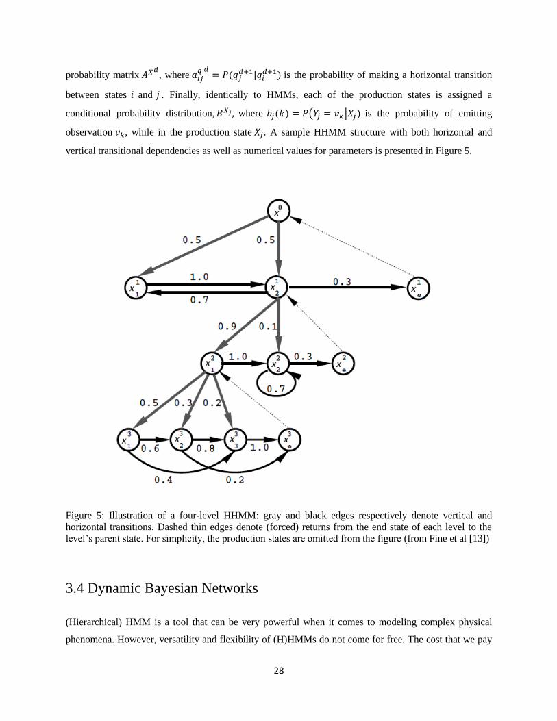
28

probability matrix , where

is the probability of making a horizontal transition

between states and . Finally, identically to HMMs, each of the production states is assigned a

conditional probability distribution, where is the probability of emitting

observation , while in the production state . A sample HHMM structure with both horizontal and

vertical transitional dependencies as well as numerical values for parameters is presented in Figure 5.

Figure 5: Illustration of a four-level HHMM: gray and black edges respectively denote vertical and

horizontal transitions. Dashed thin edges denote (forced) returns from the end state of each level to the

level’s parent state. For simplicity, the production states are omitted from the figure (from Fine et al [13])

3.4 Dynamic Bayesian Networks

(Hierarchical) HMM is a tool that can be very powerful when it comes to modeling complex physical

phenomena. However, versatility and flexibility of (H)HMMs do not come for free. The cost that we pay

29

for creating structurally complicated (hierarchical) models comes from the number of parameters that we

would have to estimate. The number of states in the model, especially in those cases when states are

marginally distinguishable, commands substantial sets of training data for the purpose of model learning.

The sample data has to be representative of the population in order to avoid bias and over-fitting. The

requirement is known as high sample complexity, and often becomes an issue when sample data is limited

or expensive to obtain. Another issue is high computational complexity at the inference stage in HMMs

[26].

In order to overcome aforementioned computational inefficiencies, an (H)HMM can be

represented as a Dynamic Bayesian Network (DBN). For details on mechanics of such transformation as

well as general description of DBNs we further refer our reader to Murphy [26], and Tayal [38]. Here we

only briefly discuss the main underlying idea. In the (H)HMM framework the joint probability

distribution of states of the hidden nodes is factored into a product of probability distribution functions of

child nodes, conditional on the state of their parent nodes, and marginal probability distributions of parent

nodes. Computational complexity of an (H)HMM comes from calculations of these conditional

probabilities. Bayesian network reveals conditional independence relations, therefore, reducing the

number of calculations that have to be performed. The idea is summarized in the principle of -

separation. Jensen et al [16] give the following definition of -separation for graphical causal nets:

“Two distinct variables and in a causal network are -separated ( for

directed graph) if for all paths between and , there is an intermediate

variable (distinct from and ) such that either

− the connection is serial or diverging and is instantiated, or

− the connection is converging, and neither nor any of ’s descendants have

received evidence.

If and are -separated, then changes in the certainty of A have no impact on

the certainty of .”

The principle of -separation reduces complexity of any given network by breaking it up into

conditionally independent subsets. Local inferences in such subsets are computationally more efficient.

Once the required computations have been performed, the subsets can be recombined back together to

form the original structure, therefore providing the same result in a computationally efficient manner.

30

Chapter 4

Trade Price and Limit Order Book -based Model

Although the idea of a double auction is straight forward, the structure and dynamics of a limit order book

might become a modeling nightmare due to multiple sources of uncertainty affecting the limit order book.

As described in Chapter 2, limit orders can be submitted on both sides of the limit order book, at different

price levels and with different supporting volumes. Such orders can be explicitly cancelled, or they can

expire. They can be executed due to price cross with new incoming limit orders, or they can transact at

the prevailing market price due to market orders. All of this can happen at random times. As pointed out

by Cont et al in [6], “given the complexity of the structure and dynamics of the order books, it has been

difficult to construct models that are both statistically realistic and amenable to rigorous quantitative

analysis”.

However, in the context of the machine learning, and DBN in particular, an order book can play a

different role and provide a different perspective. We do not attempt to come up with analytical models

for any of the aforementioned phenomena, but our objective is rather to find an aggregated metric, a

feature, that would describe the state of the order book at any given moment in time. This feature would

become a driving force behind our hierarchical hidden Markov model for modeling and predicting high-

frequency market regimes.

4.1 Volume-Weighted Average Price ( )

Multiple studies in the past have suggested that a limit order book price and volume at any given price

level might contain information that could be used to predict the direction and magnitude of the future

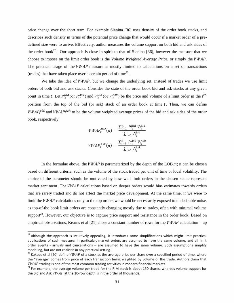
31

price change over the short term. For example Slanina [36] uses density of the order book stacks, and

describes such density in terms of the potential price change that would occur if a market order of a pre-

defined size were to arrive. Effectively, author measures the volume support on both bid and ask sides of

the order book22

. Our approach is close in spirit to that of Slanina [36], however the measure that we

choose to impose on the limit order book is the Volume Weighted Average Price, or simply the .

The practical usage of the measure is mostly limited to calculations on a set of transactions

(trades) that have taken place over a certain period of time23

.

We take the idea of , but we change the underlying set. Instead of trades we use limit

orders of both bid and ask stacks. Consider the state of the order book bid and ask stacks at any given

point in time . Let

and

be the price and volume of a limit order in the

position from the top of the bid (or ask) stack of an order book at time . Then, we can define

and

to be the volume weighted average prices of the bid and ask sides of the order

book, respectively:

In the formulae above, the is parameterized by the depth of the LOB ; can be chosen

based on different criteria, such as the volume of the stock traded per unit of time or local volatility. The

choice of the parameter should be motivated by how well limit orders in the chosen scope represent

market sentiment. The calculations based on deeper orders would bias estimates towards orders

that are rarely traded and do not affect the market price development. At the same time, if we were to

limit the calculations only to the top orders we would be necessarily exposed to undesirable noise,

as top-of-the book limit orders are constantly changing mostly due to trades, often with minimal volume

support24

. However, our objective is to capture price support and resistance in the order book. Based on

empirical observations, Kearns et al [21] chose a constant number of rows for the calculation – up

22

Although the approach is intuitively appealing, it introduces some simplifications which might limit practical applications of such measure: in particular, market orders are assumed to have the same volume, and all limit order events - arrivals and cancellations – are assumed to have the same volume. Both assumptions simplify modeling, but are not realistic in any practical setting. 23

Kakade et al [20] define of a stock as the average price per share over a specified period of time, where the “average” comes from price of each transaction being weighted by volume of the trade. Authors claim that trading is one of the most common trading activities in modern financial markets. 24

For example, the average volume per trade for the RIM stock is about 150 shares, whereas volume support for the Bid and Ask at the 10-row depth is in the order of thousands.

32

to 15 currently available limit orders in the stack. Cao et al. [4] show that the optimal depth to be used is

in the range of 2 to 10 orders. In our computations 10 orders seem to be the optimal depth25

.

LOB-based can be further illustrated based on our original example, where shares of

TSX:RIM were traded at noon on May 1, 2007. Figure 6 shows the state of the order book at 11:59 AM.

The bid at the 10-row depth is $147.50 with the corresponding cumulative size26

of 7,030 shares.

Similarly, the ask at the 10-row depth is $147.93 with the corresponding cumulative size of 4,500

shares. Figure 7 shows the state of the order book one-trade-later, at 12:00 PM with changes both in bid

and ask s and the corresponding cumulative sizes. The actual trade that took place is shown in

Figure 8.

Figure 6: State of the TSX:RIM limit order book at 11:59 AM on May 1, 2007. Outlined in blue crossed

markers are the bid and the ask prices and cumulative volume sizes calculated at 10-row depth.

Figure 7: State of the TSX:RIM limit order book at 12:00 PM on May 1, 2007. Outlined in red dotted

markers are the bid and the ask prices and cumulative volume sizes calculated at 10-row depth.

25

We have experimented with different values of . At performance of the feature appears to deteriorate. Dependency of the optimal depth on daily trading volume and volatility of the underlying stock remains to be investigated and we leave this to future research. In the following discussion we omit parameter from the formulae with the understanding that the depth is set to be constant at 10. 26

Cumulative size is the total volume included in calculation of volume weighted average price.

33

Figure 8: The Time and Sales show the trade in 100 shares of TSX:RIM at $147.68.

Figure 9: The time series of the May 1, 2007 TSX:RIM trade price, bid and ask s calculated at the

10-row depth. The blue crossed markers and red dotted markers correspond to the data points in Figures

6, 7. The plain green marker denotes the trade in Figure 8.

34

Let

be a two-dimensional stochastic process. Then the

dynamics of can serve as a proxy for the dynamics of the limit order book. Let be the trade

execution price at time . Then is a one-dimensional stochastic process. Our hypothesis is that there

is a stochastic functional dependency between the two, and that contains information that can be

used to predict movement of . We materialize the hypothesis in the Order Book Imbalance feature.

4.2 Order Book Imbalance

One can think of a limit order book as being a micro model of the market for a particular security. Ask

and Bid represent supply and demand, respectively. If we continue with the analogy, what would be a

reasonable proxy for the equilibrium market price? Silaghi et al. [35] suggest several trading strategies

based on , where an order book is thought of as an expression of market sentiment and the

price, calculated on the total order book is seen as a proxy for the market equilibrium price. The order

book-derived was also popularized by Kearns et al [21] as an indicator for the Static Order Book

Imbalance strategy. Kearns et al came up with the idea of measuring imbalance in order book stacks and

using that as a measure of the equilibrium in the market. In particular, define

and

If the market were at equilibrium (see Figure 10 for a schematic example) one would expect

and

to be the same, up to some reasonable threshold that would

exclude noise. This would imply that the market price used in the calculation of the spread and the

theoretical equilibrium price, suggested by the order book, are the same, and no market action for the

price adjustment would be expected. This does change when and

are different. If

(see Figure 11), then the actual market price is

lower than the equilibrium price suggested by the order book and one would expect the price to adjust

upwards. Intuition behind this expectation is based on a notion of volume support from technical analysis

- there is a significant volume at higher bid prices on the buy side of the order book and this would create

necessary support to the market price. On the other hand, when

,

the market price is higher than the equilibrium price suggested by the order book and one would expect

the price to adjust downwards. The intuition is that the market price would meet resistance from the sell

side of the order book, which is highly dense at the lowest ask prices.

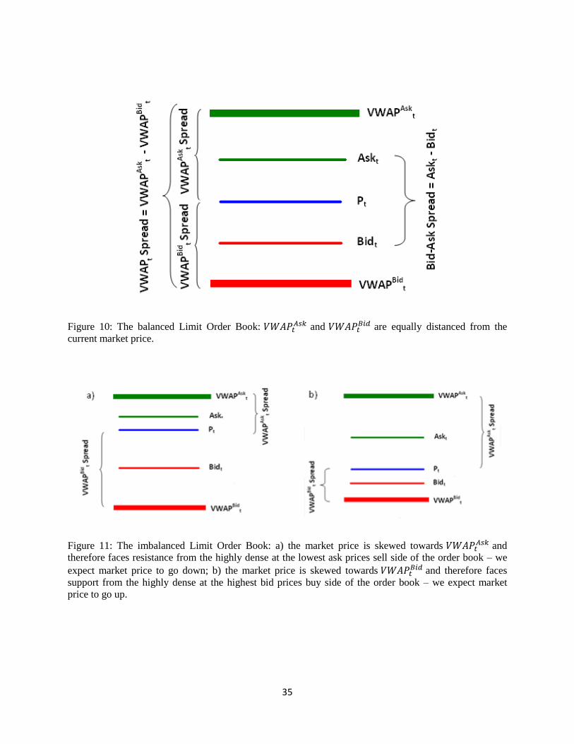
35

Figure 10: The balanced Limit Order Book: and

are equally distanced from the

current market price.

Figure 11: The imbalanced Limit Order Book: a) the market price is skewed towards and

therefore faces resistance from the highly dense at the lowest ask prices sell side of the order book – we

expect market price to go down; b) the market price is skewed towards and therefore faces

support from the highly dense at the highest bid prices buy side of the order book – we expect market

price to go up.

36

4.3 Zigzag Aggregation of Time Series

It might come as a surprise, but most often the execution price does not change from one trade to another.

Based on data used in their study, McCulloch et al [24] have found that on a high frequency level trade

price stays the same in 67% of cases. We had similar findings with the TSX60 data: on average the trade

price did not change in 65% of cases with the price being constant for more than three transactions most

of the time (see Table 2 for details). At the same time the LOB imbalance has fluctuated with every single

trade, generating trading signals for the order book imbalance model. In order to bring the two inline, an

aggregation on the time series is required. Although most transactions do not contain directional price

movement information, they, as noted in [24], certainly contribute to the intensity of trading. Moreover,

changes in the order book s over these periods of no price change can be used to model the

direction and the size of the upcoming price move. Therefore, instead of dropping out trades with no-

price-change as well as corresponding limit orders from the original time series, we follow a zigzag

approach of Lo et al [23], Tayal [38] and choose to reduce granularity to aggregate the available trade

information. Once zigzag boundaries are identified on the price series, we apply them to the order book

time series to come up with a time series of aggregated bid and ask s.

In particular, let be a sequence of local extrema extracted from the price series . Then

is the zigzag bounded by the start and end indices and in the original price

series . The series is such that for for local maxima, and for

for local minima. By construction is a time series of alternating local minima and maxima.

Individual zigzags,

, form a time series of the local extrema and its boundaries. Aforementioned

transactions with no price changes form plateaus (for local maxima) and valleys (for local minima). These

are included into adjacent zigzags, which is consistent with approach taken in Ord [27]. The alternating

nature of zigzag series achieves the desired property – the trade price changes over every step in time

series.

We illustrate these ideas on Figure 12. For this purpose we use the time series of the May 1, 2007

TSX:RIM trade price. All markers on the graph correspond to trades. The blue square markers correspond

to the plateau and the valley trades - these are the prevailing trades and they happen without change in

price, as expected. The red circle markers correspond to the end-of-zigzag trades - the zigzag local

extrema points. The green crossed circle markers correspond to the zigzag-internal trades – these trades

only contribute to the zigzags’ overall volume. We have marked boundaries for the first three zigzags

with letters , and . Zigzags and overlap in a plateau, zigzags and overlap in a valley. We

37

observe the alternating nature of the zigzag series. In particular, zigzag is a short-term up trend, zigzag

is a short-term down trend, zigzag is a short-term up-trend, and so on.

Figure 12: Time series of the May 1, 2007 TSX:RIM trade price from Figure 9. The blue square markers

correspond to the plateau and the valley trades; the red circle markers correspond to the end-of-zigzag

trades; the green crossed circle markers correspond to the zigzag internal trades.

The zigzag boundaries , established on the price series, can be applied to the limit order book

time series. The information accumulated in the order book over each zigzag run is

averaged to bring the data back to the trade price scale. In particular,

Here we note that for all , since every zigzag would include at least two trades -

these are the price points which are identified as the local extrema. The resulting time series and

are used to extract the limit order book based feature vector.

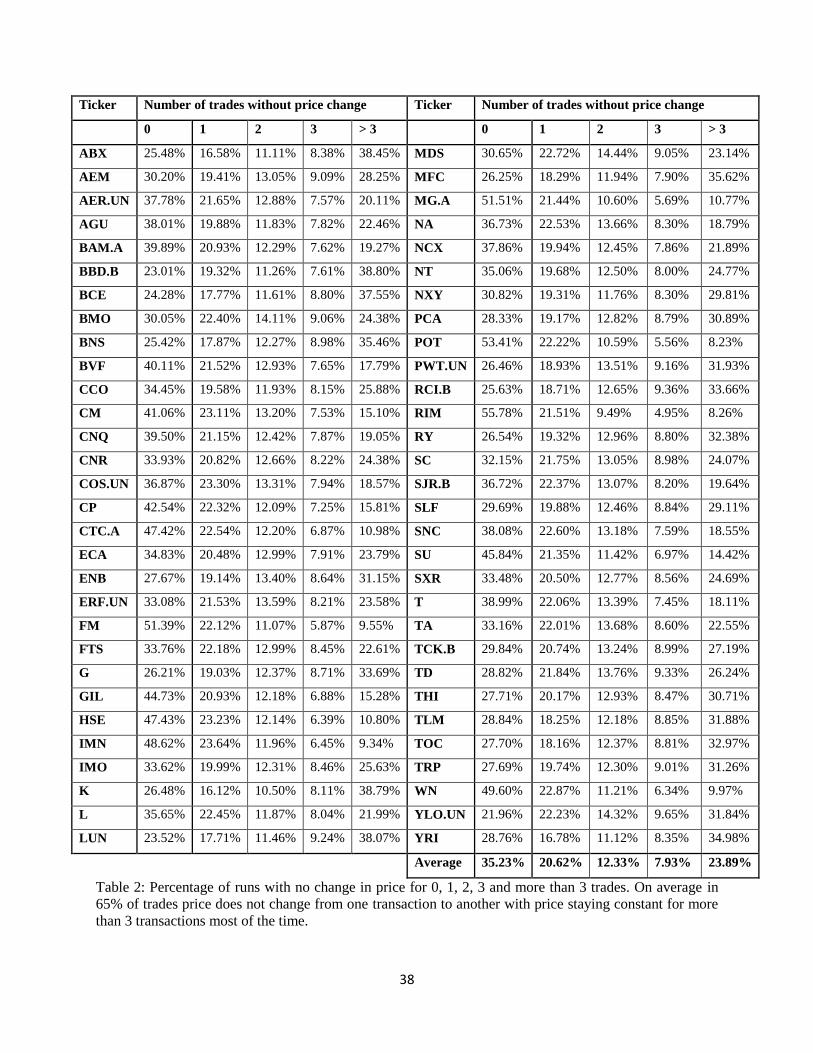
38

Ticker Number of trades without price change Ticker Number of trades without price change

0 1 2 3 > 3 0 1 2 3 > 3

ABX 25.48% 16.58% 11.11% 8.38% 38.45% MDS 30.65% 22.72% 14.44% 9.05% 23.14%

AEM 30.20% 19.41% 13.05% 9.09% 28.25% MFC 26.25% 18.29% 11.94% 7.90% 35.62%

AER.UN 37.78% 21.65% 12.88% 7.57% 20.11% MG.A 51.51% 21.44% 10.60% 5.69% 10.77%

AGU 38.01% 19.88% 11.83% 7.82% 22.46% NA 36.73% 22.53% 13.66% 8.30% 18.79%

BAM.A 39.89% 20.93% 12.29% 7.62% 19.27% NCX 37.86% 19.94% 12.45% 7.86% 21.89%

BBD.B 23.01% 19.32% 11.26% 7.61% 38.80% NT 35.06% 19.68% 12.50% 8.00% 24.77%

BCE 24.28% 17.77% 11.61% 8.80% 37.55% NXY 30.82% 19.31% 11.76% 8.30% 29.81%

BMO 30.05% 22.40% 14.11% 9.06% 24.38% PCA 28.33% 19.17% 12.82% 8.79% 30.89%

BNS 25.42% 17.87% 12.27% 8.98% 35.46% POT 53.41% 22.22% 10.59% 5.56% 8.23%

BVF 40.11% 21.52% 12.93% 7.65% 17.79% PWT.UN 26.46% 18.93% 13.51% 9.16% 31.93%

CCO 34.45% 19.58% 11.93% 8.15% 25.88% RCI.B 25.63% 18.71% 12.65% 9.36% 33.66%

CM 41.06% 23.11% 13.20% 7.53% 15.10% RIM 55.78% 21.51% 9.49% 4.95% 8.26%

CNQ 39.50% 21.15% 12.42% 7.87% 19.05% RY 26.54% 19.32% 12.96% 8.80% 32.38%

CNR 33.93% 20.82% 12.66% 8.22% 24.38% SC 32.15% 21.75% 13.05% 8.98% 24.07%

COS.UN 36.87% 23.30% 13.31% 7.94% 18.57% SJR.B 36.72% 22.37% 13.07% 8.20% 19.64%

CP 42.54% 22.32% 12.09% 7.25% 15.81% SLF 29.69% 19.88% 12.46% 8.84% 29.11%

CTC.A 47.42% 22.54% 12.20% 6.87% 10.98% SNC 38.08% 22.60% 13.18% 7.59% 18.55%

ECA 34.83% 20.48% 12.99% 7.91% 23.79% SU 45.84% 21.35% 11.42% 6.97% 14.42%

ENB 27.67% 19.14% 13.40% 8.64% 31.15% SXR 33.48% 20.50% 12.77% 8.56% 24.69%

ERF.UN 33.08% 21.53% 13.59% 8.21% 23.58% T 38.99% 22.06% 13.39% 7.45% 18.11%

FM 51.39% 22.12% 11.07% 5.87% 9.55% TA 33.16% 22.01% 13.68% 8.60% 22.55%

FTS 33.76% 22.18% 12.99% 8.45% 22.61% TCK.B 29.84% 20.74% 13.24% 8.99% 27.19%

G 26.21% 19.03% 12.37% 8.71% 33.69% TD 28.82% 21.84% 13.76% 9.33% 26.24%

GIL 44.73% 20.93% 12.18% 6.88% 15.28% THI 27.71% 20.17% 12.93% 8.47% 30.71%

HSE 47.43% 23.23% 12.14% 6.39% 10.80% TLM 28.84% 18.25% 12.18% 8.85% 31.88%

IMN 48.62% 23.64% 11.96% 6.45% 9.34% TOC 27.70% 18.16% 12.37% 8.81% 32.97%

IMO 33.62% 19.99% 12.31% 8.46% 25.63% TRP 27.69% 19.74% 12.30% 9.01% 31.26%

K 26.48% 16.12% 10.50% 8.11% 38.79% WN 49.60% 22.87% 11.21% 6.34% 9.97%

L 35.65% 22.45% 11.87% 8.04% 21.99% YLO.UN 21.96% 22.23% 14.32% 9.65% 31.84%

LUN 23.52% 17.71% 11.46% 9.24% 38.07% YRI 28.76% 16.78% 11.12% 8.35% 34.98%

Average 35.23% 20.62% 12.33% 7.93% 23.89%

Table 2: Percentage of runs with no change in price for 0, 1, 2, 3 and more than 3 trades. On average in

65% of trades price does not change from one transaction to another with price staying constant for more

than 3 transactions most of the time.

39

4.4 Model Specification and Feature Vector Extraction

When deciding on a model for any real life phenomena one should be aware of two major pitfalls: the in-

sample over-fitting and the model oversimplification. In-sample over-fitting happens when a chosen

model closely replicates patterns in data at hand, but fails to recognize data characteristics out of the

sample. Such models are often fairly complicated parametric models that involve distributional

assumptions as well as the estimation of the required parameters on a limited sample data. There exist

numerous examples when sound complicated theoretical models fail in practice27

. Oversimplified models,

on the other hand, fail to distinguish vital characteristics in the sample data. Such models might be

analytically tractable and fairly easy to estimate, but would fail to reflect the reality and would lack any

meaningful predictive power. Finding a balance between the two extremes is as much of an art as it is of a

science, and requires thorough knowledge of the problem’s domain and ability to introduce

simplifications without affecting usability of the model. In case of graphical probabilistic models, such as

Hidden Markov Models, knowledge of problem’s domain translates into the topology of the model and a

feature vector that accurately reflects the characteristics of the time series data.

An investment doctrine used by quantitative hedge funds - active money management - is

primarily based on alpha trading models28

. These models effectively reject Efficient Market Hypothesis

and exploit market inefficiencies, such as temporary mispricing of financial instruments, limited or

absence of liquidity, etc. 29

. The underlying hypothesis for the majority of alpha models, which include

mean-reverting models, such as statistical arbitrage, and trend following models, is that short, medium,

and long term trends exist in financial markets. Therefore, we speculate that a successful alpha trading

model must incorporate runs and reversals. Indeed, regime switching models have been widely used for

financial price modeling (for multiple examples see [41]). The usefulness of such models is established

based on their ability to identify bull and bear regimes. Clearly, the task is daunting – indicators that can

help with a reliable identification of the current and future trends simply do not exist. We believe that a

hidden Markov model has the potential in modeling and generating signals for regime switching.

27

For example, in portfolio construction, theoretically sound mean-variance optimization is built entirely on assumption of availability of reliable estimates for large number of parameters to yield meaningful results. However, parameters, such as mean returns, are impossible to estimate with a necessary level of precision. 28

Active money management is different from static money management used by the majority of mutual funds, which employ beta-models, like CAPM, and passively invest in market as a whole, or a particular industry sector with the intention of getting only the beta exposure. 29

Such strategies have proven to be robust and profitable. For example, Theory of Reflexivity, popularized by the famous speculator George Soros in his “Alchemy of Finance” is based on existence of trends [37].

40

Figure 13: Time series of the May 1, 2007 TSX:RIM trade price. The solid red lines correspond to the

trends identified at high retracement levels; the double green line corresponds to trends identified with

lower retracement levels.

Typically, price trends persist for prolonged periods of time. In macro-driven trading, this can

mean weeks, months, and even years. In high frequency trading, a trend can exist only for minutes or

hours, but would still correspond to multiple trades and zigzags, and therefore be considered a trend on

the relevant time scale. Trend identification typically involves specification of a retracement level. The

retracement level defines the minimum that the price is required to deviate from the most recent extrema

in the opposite direction before a run is relabeled as a reversal, and vice versa. Therefore, the retracement

level defines a scale to be used to measure trends. In Figure 13 we present the time series of the May 1,

2007 TSX:RIM trade price with the two series of the possible price trends. The solid red lines correspond

to the trends identified at high retracement levels (therefore low frequency of trend switching). The

double green line corresponds to trends identified with lower retracement levels (high frequency of

switching).

Regardless of how low the retracement level is, one would still expect to see short term

deviations from the general trend. At the ultra high frequency level these are known as bid-ask bounce.

The phenomenon is well-studied and documented in the academic literature (see for example [24]).

Therefore, any long-term macro trend (either upward or downward) is expected to have short-lived micro

41

trends that do not change labeling of the trend as a run or reversal based on the specified retracement

level, but at the same time work in the opposite direction to the general trend. These are embedded in the

price time series. By construction of the zigzag time series, individual zigzags can be identified with

short-term micro trends30

. Based on the discussion above, we contemplate that a successful alpha model

should take into account identifiable micro-trends at the level of observations. Clearly, short-term micro-

trends exist in both run and reversal regimes; therefore it seems appropriate to consider a symmetric

topology for such model. Figure 14 shows topology of a hypothetical model.

Figure 14: A schematic representation of a graphical model that incorporates our knowledge about the

existence of runs and reversals as well as short-lived micro trends within those runs and reversals.

The existence of the short term trends could be interpreted as local noise and therefore the

corresponding continuous time model of price development in the run and reversal regimes could be of

the form

30

In the context of our study, the bid-ask bounce of the trade price is treated as a Brownian motion. In our data structure, these correspond to zigzags. We argue that price series when analyzed at the high frequency zigzag level does not contain any consistently useful information to base the trading on.

42

where is the asset price, is a standard Wiener process, is the volatility term, and is the drift

term which at any given point in time takes on one of two values, or , that are necessarily different

for the run and reversal regimes. Effectively, the price development in the two regimes is driven by the

two processes which have the same stochastic factor, but different drift terms. The regime switching is

based on a stochastic process, taking the value of 1 or 2 at any time 31.

A simple topology of a hierarchical hidden Markov model proposed by Tayal [38] incorporates

hidden market states identified above. The structural symmetry of different market regimes has been

preserved as well. In addition, the proposed conditional dependencies between different interior states,

vertical and horizontal transactions within the HHMMs structure are also appealing. Therefore we adopt

this model in our study. Since our goal is to study predictive power of the limit order book, we need to

incorporate the LOB info into the feature vector appropriately. Using the same structure for the model

would also allow us to perform unbiased comparative analysis of the computational results produced by

the volume and limit order book models.

The HHMM under consideration contains three hidden levels32

. At the top level there is a single

root node . Its presence is required only for the initial vertical transition to one of the mid-level internal

states, and

, which represent run and reversal regimes in the market. Each of these internal states is a

probabilistic model, which consists of two production states that emit observations, and a termination

state that allows for the vertical transition back to the mid-level internal states. The short-term micro-

trends, represented in terms of zigzags, are used as the observable output of the model. The model’s

topology is symmetric: each of the child models allows for emissions of positive observations (zigzags

containing local maxima) via the production nodes and

and negative observations (zigzags

containing local minima) via the production nodes and

Once activated, each child model alternates

between positive and negative production nodes, until a termination node is entered which automatically

triggers a vertical transition back to the mid-level internal state, followed by a forced horizontal

transaction to another child model as there are no internal loop-backs. Termination nodes in both child

models are identical. Their sole purpose is to return control back to the parent node in the mid-level. We

should note that a horizontal transition from the production state emitting positive (negative) zigzag

31

The regime switching process can be modeled using different approaches. For example, Chen et al [5] label the two market regimes as 0 and 1, and use a two-state continuous-time Markov chain , represented by

,

where “ - is the time infinitesimally before , and and are the independent Poisson processes with intensity and respectively”. ( denotes the probability of shifting from regime 0 to regime 1 over a small time interval , and is the probability of switching from regime 1 to regime 0 over ). 32

The discussion will closely follow that of Tayal [38], unless otherwise noted. Refer to Figure 15 for details on the model.

43

observations is necessarily followed by either a production state emitting negative (positive) zigzag

observations, or a terminating state. At the lowest level positive and negative production nodes alternate

between each other. This way the model preserves alternating order of the zigzag sequences – there are no

loopbacks on either positive or negative emitting nodes. Even when there is a transition between the two

mid-level models, the alternating order of emissions is preserved. The model of can only be terminated

from a node which emits negative zigzag observations, and the first observation after termination

node is necessarily produced by the production state emitting positive zigzag observations,

Similarly, the model of can only be terminated after emitting a positive observation from the

production node and the first observation after the termination node

is necessarily produced by the

production state emitting negative zigzag observations, . We shall see later how this restriction is

enforced via the state transition probability matrix.

Figure 15: The Hierarchical Hidden Markov model of the price and limit order book; and

are the

top level hidden states representing the run and reversal regimes in the market; and

represent

negative zigzags, whereas and

represent positive zigzags. The production nodes are filled in grey

colour; the lowest level transition nodes enforce the alternating sequence of the positive and negative

zigzags (from Tayal [38]).

The initial vertical transition through the model is guided by the probability distribution function

where is the hierarchy level index, For the root node, we define

; for the mid-level internal states

and the vertical transition is restricted to

44

the production states and

respectively, and therefore the probability functions are defined as

and

, respectively.

As mentioned earlier, neither of the child models allows internal loop-backs; therefore once a

child model enters a termination state, there is a horizontal transition between the mid-level models. This

is signified by the top-level state transition probability matrix,

At the production state level, state transition probabilities are defined as

and

Finally, each of the production states

and

is parameterized by an observation

probability function

, where

is the probability of emitting observation

symbol , while in the producton state

Once the topology of the model is established, and conditional dependences and transition flows

are identified, our focus shifts to the feature vector. The essence of the task is to extract information from

the data, such that the model would be able to classify short-term micro trends and identify them with

particular hidden regimes33

. The most natural starting point for such a search is the price time series. It

can provide insight into the direction of the price change (up or down), as well as the persistence on the

33

The big question that the model should answer can be formulated as following: “Given the information extracted from data in the form of a feature vector, does the short-term up micro trend belong to a run or a reversal state of the market?” Same question is asked for a given short-term down micro trend.

45

price action - whether the price has risen or fallen over a sequence of time steps, such as zigzags.

Furthermore, one could look for the strength of the price action by imposing threshold limits on the price

difference. Breaking through the threshold could signal a trend formation, whereas any price change

below the threshold could be recognized as noise. Support for trends identified in the price time series

could also be found in other data sources. Probably most widely used is the volume time-series.

Numerous studies have been conducted on the topic, primarily by followers of the technical analysis34

.

This topic has been studied in the academic literature as well. Tayal [38] has been successful in extracting

price and volume information: the model used by the author demonstrated superior results both in- and

out-of-sample. Our current study echoes that of Tayal in terms of using price time series for the purpose

of identifying the direction of the price development and trends. However, trend supporting information is

extracted from the limit order book data. We describe the feature vector based on the trade price and LOB

feature next.

We start by noting that has been defined as a time series of individual zigzags, and

contains information necessary to construct the following feature vector,

The first two components of the feature vector are based strictly on the price exrema, , and

therefore mimic those of Tayal [38]. In particular,

The definition of the direction component, , is simple –

zigzag is either positive or

negative. Some variation in the trending component, , is possible, although the definition above

presents itself as the most plausible since (i) it captures the trending information in the price time series,

34

See references to [38] for an extensive list of literature.

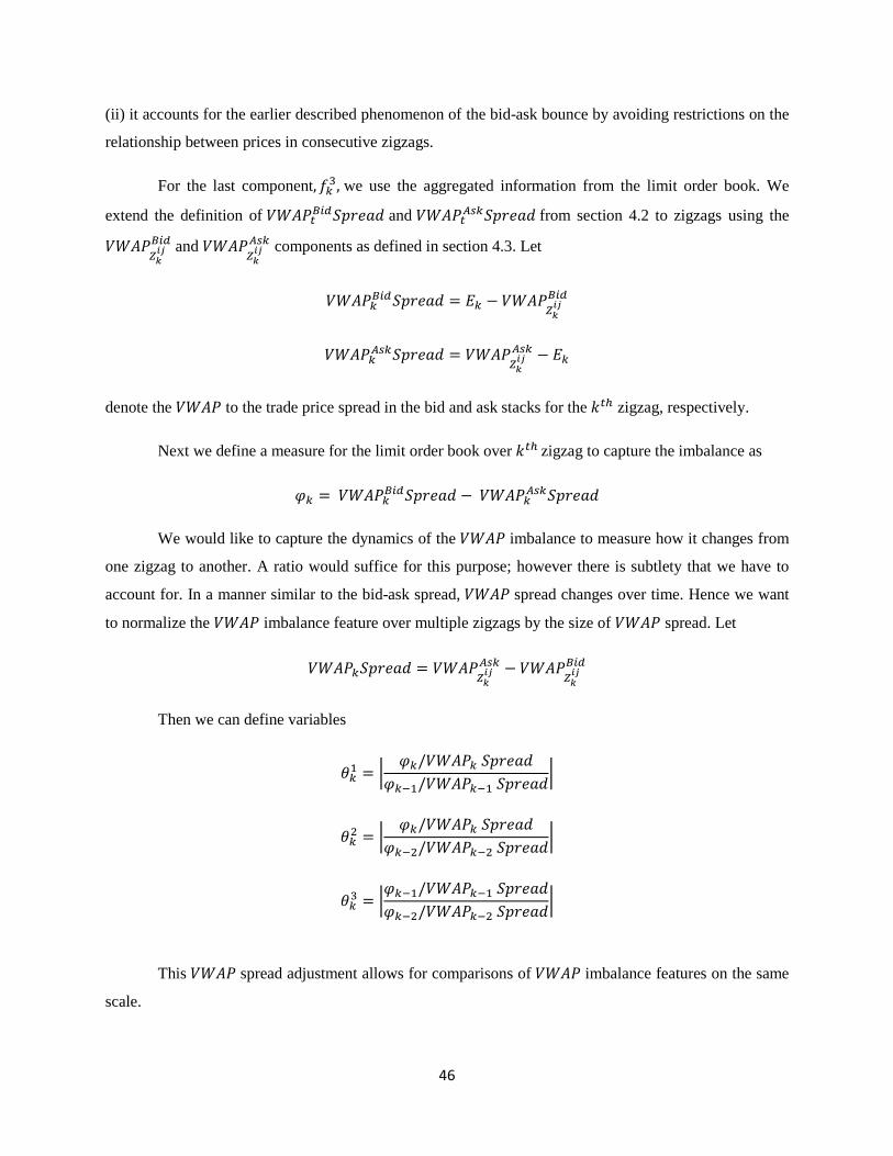
46

(ii) it accounts for the earlier described phenomenon of the bid-ask bounce by avoiding restrictions on the

relationship between prices in consecutive zigzags.

For the last component we use the aggregated information from the limit order book. We

extend the definition of and

from section 4.2 to zigzags using the

and

components as defined in section 4.3. Let

denote the to the trade price spread in the bid and ask stacks for the zigzag, respectively.

Next we define a measure for the limit order book over zigzag to capture the imbalance as

We would like to capture the dynamics of the imbalance to measure how it changes from

one zigzag to another. A ratio would suffice for this purpose; however there is subtlety that we have to

account for. In a manner similar to the bid-ask spread, spread changes over time. Hence we want

to normalize the imbalance feature over multiple zigzags by the size of spread. Let

Then we can define variables

This spread adjustment allows for comparisons of imbalance features on the same

scale.

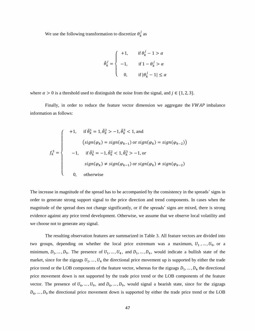
47

We use the following transformation to discretize as

where is a threshold used to distinguish the noise from the signal, and .

Finally, in order to reduce the feature vector dimension we aggregate the imbalance

information as follows:

The increase in magnitude of the spread has to be accompanied by the consistency in the spreads’ signs in

order to generate strong support signal to the price direction and trend components. In cases when the

magnitude of the spread does not change significantly, or if the spreads’ signs are mixed, there is strong

evidence against any price trend development. Otherwise, we assume that we observe local volatility and

we choose not to generate any signal.

The resulting observation features are summarized in Table 3. All feature vectors are divided into

two groups, depending on whether the local price extremum was a maximum, or a

minimum, . The presence of , and , would indicate a bullish state of the

market, since for the zigzags the directional price movement up is supported by either the trade

price trend or the LOB components of the feature vector, whereas for the zigzags the directional

price movement down is not supported by the trade price trend or the LOB components of the feature

vector. The presence of , and , would signal a bearish state, since for the zigzags

the directional price movement down is supported by either the trade price trend or the LOB

48

components of the feature vector, whereas for the zigzags the directional price movement up is

not supported by the trade price trend or the LOB components of the feature vector. The zigzags

capture local volatility noise as the direction of the price movements does not find support in

either the trade price trend or in the LOB feature vector components.

Table 3: The trade price and Imbalance feature space (from Tayal [38]).

The objective of the model is to identify hidden states based on the sequence of observations. If

our hypothesis is correct and the limit order book information combined with the price signals can be

used to identify hidden states (trends) in the market, then we would expect to be able to build a profitable

trading strategy based on the information about the inferred hidden states. We discuss whether the model

is successful in doing so in the next chapter.

49

Chapter 5

Computational Results

In this chapter we describe the data used in our numerical experiments, and present some preliminary

computational results from the price and limit order book model. In addition, we assess its statistical

significance. We further perform comparative analysis of our results with the results of a simple daily buy

and hold trading strategy as well as the results produced by the price and volume model. We start with a

description of the Limit Order Book Analyzer – the software tool that we have built to navigate the tick-

by-tick trade and the limit order book data, and to calculate the component of the feature vector.

5.1 Limit Order Book Analyzer

The quality of the input data is of a paramount importance to the success of any applied statistical study.

In general, researchers employ a number of techniques to ensure the quality of the data. Simple visual

inspections of data using a variety of plotting techniques and calculation of basic sample statistics are

often sufficient for this purpose.

The challenge presented by the high-frequency data lies in its sheer amount, which makes manual

data cleaning and validation almost impossible35

. At the same time, such data is often very well

structured, therefore making it a perfect candidate for machine-processing. We have built a Limit Order

35

The data used in our study serves as a good example of how vast the high-frequency data can be – the text files with day-worth of order and trade records have an average size of 1 Gb each.

50

Book Analyzer, which has greatly helped us navigate the tick-by-tick trade and the limit order book data,

and calculate the component of the feature vector. We present a snapshot of the LOB Analyzer in

Figure 16.

The choice of the programming language is dictated by the requirements of computational

efficiency and by the presence of graphical user interface (GUI) library. Any of the compiled languages

would serve the task of efficiency well. However, some of the most computationally efficient languages,

such as C++, lack a universal GUI library. Therefore, we have opted to use the Java programming

language, which offers Swing widget toolkit as part of the Sun Microsystems’ Java Foundation Classes36

.

High-level design of the application follows the classic Model-Viewer-Controller architectural

pattern. Internally the application is built of the four main blocks: the data processing block, the user

interface (UI) block with the control panel, the block for the internal models of the limit order book and

the time and sales, and the block for the calculation of the feature vector.

The data processing block is designed for processing of the raw input data, which is read from the

comma-delimited text files. This block is abstracted from the rest of the application, so that the LOB

Analyzer is not dependent on any particular data source or data format. This way the LOB Analyzer can

be easily adapted to process data from other sources, like databases.

The UI is comprised of the limit order book stacks, the time and sales, the control panel, and the

output panel for error and warning messages. The application is managed by a user via the control panel,

which is comprised of the Settings and Controls panes. The Settings pane is used at the startup time to

specify ticker and raw data file information. The Controls pane is used both at the startup time and during

the application run time. User has the option to specify whether the application should run in automatic

mode either until the next record, or the next trade, or the particular time during the day, or the end of the

day, or the end of the available ticker data. At any moment during the run time, user can pause the

execution, and capture the state of the limit order book and the time and sales panes, as well as calculate

statistics of interest based on this snapshot in time.

Internally, the limit order book is represented by a class which maintains a list of buy limit orders

and a list of sell limit orders and encapsulates the functionality for order insertion and order removal as

well as calculation of the volume-weighted average price. The time and sales model maintains a list of

executed trades.

36

Portability of Java applications came as a bonus.

51

Figure 16: A snapshot of the Limit Order Book Analyzer tool. The Time and Sales pane displays most

recent trades with the price and volume information, the corresponding buy and sell orders and the total

volume traded on the day. The Bid and Ask stacks display buy and sell limit orders, order ids, time when

the orders were submitted, the size of the orders, the limit prices, the volume-weighted average prices and

the cumulative volumes used in the calculation.

52

Finally, there is a feature vector calculation block, which encapsulates the logic for calculation of

the zigzag time series following the feature vector definition provided in section 4.4. It is fairly easy to

calculate the price direction and the magnitude components of the feature vector directly from the trades

data, as such calculation depends only on time, and the trades data is chronologically ordered. However,

the component of the feature vector requires calculations on the order book stacks, which are

ordered first based on the limit price and only then on the time of the order arrival. This presents a

challenge that would be hard to overcome without the LOB Analyzer.

5.2 Data Set

The data used in our analysis is obtained from the Toronto Broadcast Feed. The original raw data contains

records for 278 tickers that were traded on the Toronto Stock Exchange in May of 2007. We choose to

perform our analysis only on the actual constituents of the TSX60 index at that time. These are the largest

companies traded on the Toronto Stock Exchange as measured by their market capitalizations. The

filtered TSX60 records are aggregated by the date, giving us 22 source text files of the streamed data to

work with based on the number of trading days, excluding weekends and holidays. All the records come

chronologically ordered with by-the-second precision. The date and time, as well as the ticker information

are present in each record. We check every record for the matching date. Those records for which the date

does not match the file time stamp are discarded. Cross trades are removed from the data37

. Potential

crosses (the same broker id, and one of the limit orders is found on either side of the limit order book) are

not considered to be crosses; such records are left in the data.

Each record is classified as either a buy order or a sell order, or a trade report. Every buy or sell

order record in the data is either a booking of a new order or a cancellation of an existing one. Other types

of order records, such as Accepted and Pending, are also encountered in the data. Such records are

discarded from the data set as they designate transitional states and are later confirmed by the Booked and

Cancelled records. The total number of such records is found to be less than 0.005% of all the records.

Booked and Cancelled order records contain the volume information, recorded as the number of shares to

be bought or sold. In the current study we concentrate on the analysis of the day orders, therefore good-

till-canceled orders are removed from the data set. This is not expected to significantly affect the results,

as the total number of trades carried over from one trading day to the next in our dataset is found to be

37

Cross trades are those for which both the buy order and the sell order are originated from the same brokerage, but neither one of those orders is recorded in the limit order book. Corresponding trades are propagated to the exchange, but they do not affect the market price.

53

less than 1%. The Booked order records contain the price information as well as the record identification

number, which is a combination of the identification number of the brokerage firm from which the order

is originated and a unique order identification number. The Cancelled order records contain information

about the original order identification number and the time stamp of the original booking record. Booking

order ids are brokerage-unique up to a trading day. The Booked orders include new orders as well as re-

booked orders, with the latest being the case when either the price or volume information of the original

order change.

Trade reports contain the volume and price information for the trades, as well as the information

about the original buy and sell orders that are matched by this trade. The original buy and sell order

identification numbers and the time stamps are included with each trade report record. In addition, these

records contain information about the volume remaining in the original buy and sell orders after the

current trade. Although this information can be deduced directly from the original order and trade

volume, it serves as a good check in data cleaning and in the order book reconstruction process. If the

remaining volume of a limit order is equal to zero, such an order is removed from the LOB stack.

5.3 Learning the Model from the Data

The Limit Order Book Analyzer application is used to process the raw data and generate zigzag-based

feature vectors. There are 724,067 zigzags in the TSX60 sample data, with half of zigzags containing

local minima, and another half – local maxima. There are 362,020 zigzags and 362,047 zigzag

occurrences; this almost equal division is expected since by construction an up-zigzag is followed by a

down-zigzag, and vice-versa. As demonstrated in Figure 17, the distribution within each sub-group

follows similar pattern, with the majority of zigzags (about 64%) falling into the feature buckets and

, in which case there is no price trend and no limit order book signal to support the changing trade price

(see Table 3 in section 4.4. for the details of the feature vector specification). This does not come as a

surprise - we would expect the majority of the price changes to be driven by the local volatility, and only

a minor portion of the price changes to provide the actual trend signal, rather than the price action noise.

Another interesting observation is that the distribution of zigzags is skewed. In particular, we see a large

number of observations with the matching direction and the LOB imbalance components, but without the

trend support ( and ); at the same time there are fewer observations with the mismatching direction

and the LOB components ( and ). The immediate conclusion out of this observation is that there is a

positive correlation between the price direction and the order book imbalance. The occurrences of the

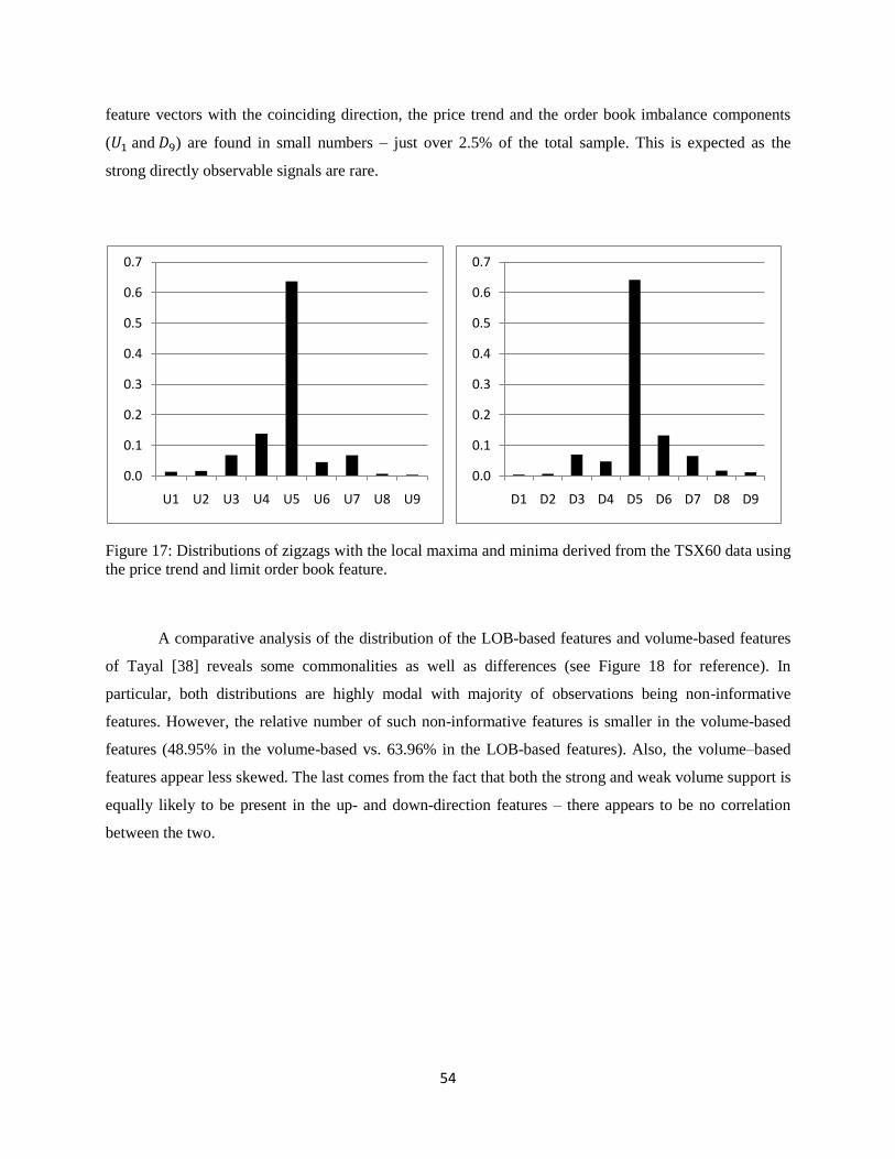
54

feature vectors with the coinciding direction, the price trend and the order book imbalance components

( and ) are found in small numbers – just over 2.5% of the total sample. This is expected as the

strong directly observable signals are rare.

Figure 17: Distributions of zigzags with the local maxima and minima derived from the TSX60 data using

the price trend and limit order book feature.

A comparative analysis of the distribution of the LOB-based features and volume-based features

of Tayal [38] reveals some commonalities as well as differences (see Figure 18 for reference). In

particular, both distributions are highly modal with majority of observations being non-informative

features. However, the relative number of such non-informative features is smaller in the volume-based

features (48.95% in the volume-based vs. 63.96% in the LOB-based features). Also, the volume–based

features appear less skewed. The last comes from the fact that both the strong and weak volume support is

equally likely to be present in the up- and down-direction features – there appears to be no correlation

between the two.

0.0

0.1

0.2

0.3

0.4

0.5

0.6

0.7

U1 U2 U3 U4 U5 U6 U7 U8 U9

0.0

0.1

0.2

0.3

0.4

0.5

0.6

0.7

D1 D2 D3 D4 D5 D6 D7 D8 D9

55

Figure 18: Distributions of zigzags with the local maxima and minima derived from the TSX60 data using

the price trend and volume feature.

The zigzag-based feature vector time series generated by the limit order book analyzer represents

observations in the price and limit order book model; they are used to learn model parameters and

perform in- and out-of-sample inferences. Following Tayal [38], we restrict in-sample learning to a

rolling window of five days of data and use the Baum-Welch (EM) algorithm to learn model parameters,

identify and classify hidden states as runs and reversals. As an alternative, one could manually label the

hidden states based on the subjective beliefs about what level of price change (a retracement level) is

required to signal a switch from a bullish market regime (a run) to a bearish market regime (a reversal),

and vice versa. Although such an approach is used by a number of technical price trend indicators, it

introduces a possibility of mislabeling hidden states, as the same zigzag could be considered to be part of

a run or a reversal, depending on the magnitude of the retracement level chosen. The EM learning

methodology appears to be a more robust and therefore a preferable approach to identify regime

switching. Once optimal boundaries for the hidden states have been identified using the Baum-Welch

(EM) algorithm and the inference mechanism, it is then trivial to decide which state is bullish and which

is bearish based on the in-state expected returns. In particular, let the expected trade returns in a hidden

state , be

0.00

0.10

0.20

0.30

0.40

0.50

0.60

U1 U2 U3 U4 U5 U6 U7 U8 U9

0.00

0.10

0.20

0.30

0.40

0.50

0.60

D1 D2 D3 D4 D5 D6 D7 D8 D9

56

where

and

are, respectively, the trade prices at the beginning and the end of the series of zigzags

which comprise state , and is the number of such sequencies attributed to state

. Then state is

bullish and is bearish if

, or

is bearish and is bullish if

.

The learned model parameters – the distributions of zigzags, conditional on the hidden states –

are demonstrated in Figure 19. The shapes of these distributions are intuitively appealing. One would

expect to see a higher number of the bullish zigzag features ( and ) with a steadily

increasing price and imbalance support from the bid stack of the limit order book during the run market

regimes. Similarly, the bearish zigzag features ( , and ) with the consistently decreasing

price and imbalance resistance from the ask stack of the order book would be prevailing in the reversal

regimes. The distinction between the two different regimes visually appears to be less pronounced than

that of the price trend and volume feature in Tayal [38]. For reference purpose, we provide graphs of

conditional distribution of price trend and volume feature in Figure 20.

Figure 19: Distributions of zigzags conditional on the hidden state, aggregated over a 5-day rolling

window – the price trend and LOB feature.

0.0

0.1

0.2

0.3

0.4

0.5

0.6

0.7

U1 U2 U3 U4 U5 U6 U7 U8 U9

RunReversal

0.0

0.1

0.2

0.3

0.4

0.5

0.6

0.7

D1 D2 D3 D4 D5 D6 D7 D8 D9

RunReversal

57

Figure 20: Distributions of zigzags conditional on the hidden state, aggregated over a 5-day rolling

window – the price trend and volume feature.

5.4 Out-of-Sample Inference

The model that we have learned can be used for multiple purposes – a comprehensive list of tasks, which

can be performed by such a model, is presented by Murphy [26]. For the purpose of this study we are

particularly interested in the predictive power of our model out of sample. In particular, we would like to

assess the model’s ability to predict the sequence of hidden states

, given the history of

zigzag observations and the model’s parameters. The resulting sequence of hidden states

is Viterbi-optimal as discussed in section 3.2.4. Formally, we can define the problem as

follows:

where

If our model is successful in identifying such upcoming hidden states, we could devise a number of

profitable trading strategies. The simple strategy that we employ in our further analysis is to buy at the

0.00

0.10

0.20

0.30

0.40

0.50

0.60

U1 U2 U3 U4 U5 U6 U7 U8 U9

Run Reversal

0.00

0.10

0.20

0.30

0.40

0.50

0.60

D1 D2 D3 D4 D5 D6 D7 D8 D9

Run Reversal

58

beginning and sell at the end of the run regime, but sell at the beginning and buy at the end of the reversal

regime38

.

The inferred regimes of each of the top level states can be used to generate the out-of-sample

returns. Such returns are calculated as a ratio of the difference between the price at the end and the

beginning of the regime divided by the price at the beginning of that regime, regardless of the regime’s

time length. Since the individual realizations of the run and reversal regimes are of different time lengths,

the resulting time series of the returns is non-synchronous. We normalize the series by scaling each return

by the length of the regime for which it was calculated. The resulting normalized return series is used to

obtain the annualized returns. We calculate the following annualized trade returns for each ticker: (i)

which is the return cumulatively generated in all the states identified as the run regime, (ii)

which is the return cumulatively generated in all the states identified as the reversal regime, and

(iii) , which is the total return generated by the trading strategy, = 39. Our further

analysis of the out-of-sample computational results is based on these annualized trade returns. Using the

resulting sets of the annualized returns for the TSX60 index constituents, we study two problems of

interest.

First, we compare the total returns to the benchmark returns . We choose a simple buy

and hold daily trading strategy as our benchmark: a security is bought at the start of the trading, and sold

with the closing bell; both transactions happen at the prevailing market prices and yield daily returns.

Second, we establish whether our model is successful in learning two distinct market regimes. For

this purpose we compare the returns in the run regime, , to the returns in the reversal regime . If

the returns are consistently different, we would be able to conclude that they are generated in different

market regimes, which our model is able to identify.

We study the above problems in the context of liquidity. Following Tayal [38], we assess how

liquidity of the underlying ticker affects predictive ability of our model and profitability of the trading

strategy. It is a common practice to proxy liquidity of publicly traded stocks with their average daily

38

In a real world environment profitability of the LOB-trading strategy would depend on its capacity. This is a large topic on its own and it is therefore beyond scope of the current study. It should be noted that expected returns are calculated under the assumption that the market would not significantly change if our trading strategy were to contribute limit orders to the market. This might be a realistic assumption for high average daily volume stocks. 39

Total return definition that we use for the analysis implies that the trading strategy takes a long position in the underlying instrument during the bull regimes and a short position in the underlying instrument during the reversal regimes. This way, for example, negative returns in reversal regimes yield positive contributions to the total returns.

59

trading volumes40

. Therefore we divide our sample into four groups listed in Table 4, based on the

average daily trading volume.

Once the sample data is split into four groups, we calculate returns generated by the trading

strategy based on the LOB model41

over the course of the 17 out-of-sample days, as well as calculate

returns of the simple B&H strategy. The sample summary statistics of these returns are presented in Table

5. The total return generated by the LOB strategy at 23.80% is higher than the benchmark return of the

B&H strategy at 6.63%. However this relation is not consistent throughout liquidity quartiles. The

performance of the B&H strategy steadily improves from the 1st Quartile to the 4

th Quartile. On the

opposite, the performance of the LOB strategy deteriorates along with the disappearing liquidity. These

findings are consistent with those of Tayal [38] – the high-frequency regime based models thrive in the

highly liquid market environment and struggle to perform well when the trading volume is low. The

distributions of the returns appear to be asymmetric, which is supported by the skewness numbers. The

standard deviations of the annualized returns per quartile are mixed.

1st Quartile 2nd Quartile 3rd Quartile 4th Quartile

Ticker Vol (MM) Ticker Vol (MM) Ticker Vol (MM) Ticker Vol (MM)

SJR.B 22.6 MFC 2.1 YLO.UN 1.24 IMO 0.59

TOC 10.5 CCO 1.99 TRP 1.18 CP 0.56

BCE 9.4 RY 1.98 T 1.17 SC 0.56

BBD.B 5.06 ABX 1.96 BAM.A 1.03 NA 0.54

MG.A 4.7 PCA 1.91 TA 1.02 SNC 0.52

G 4.11 YRI 1.85 MDS 0.91 BVF 0.5

SXR 3.95 CNR 1.78 SLF 0.91 FM 0.45

TLM 3.78 BNS 1.73 HSE 0.85 L 0.45

LUN 3.53 RCI.B 1.54 POT 0.83 NCX 0.44

CTC.A 3.4 RIM 1.48 AEM 0.79 THI 0.4

K 3.32 COS.UN 1.43 AGU 0.77 GIL 0.38

SU 2.92 BMO 1.36 ENB 0.72 FTS 0.33

TCK.B 2.7 TD 1.3 CM 0.65 ERF.UN 0.32

ECA 2.23 CNQ 1.29 AER.UN 0.65 IMN 0.29

NXY 2.19 NT 1.27 PWT.UN 0.62 WN 0.13

Table 4: The quartile groupings of the TSX60 tickers by the average daily volume

in the month of April 2007 (from Tayal [38]).

40

Risk management and portfolio analysis tools in trading systems such as Bloomberg use average daily volume as a simple way of measuring liquidity. 41

From now on this strategy is referred to as the LOB strategy.

60

(a) (b)

(c) (d)

Figure 21: The value of $1 invested in the four quartiles of different liquidity for the month of May 2007:

(a) 1st Quartile – (d) 4

th Quartile

0.88

0.9

0.92

0.94

0.96

0.98

1

1.02

1.04

1.06

1.08

1.1

Buy & Hold

LOB

0.985

0.99

0.995

1

1.005

1.01

1.015

1.02

1.025

1.03

Buy & Hold

LOB

0.98

0.985

0.99

0.995

1

1.005

1.01

1.015

1.02

1.025

1.03

Buy & Hold

LOB

0.98

0.99

1

1.01

1.02

1.03

1.04

Buy & Hold

LOB

61

B & H LOB

Mean Std Skew Mean Std Skew

1st Quartile -40.50% 112.80% -0.11 82.00% 159.79% 1.44

2nd Quartile 13.24% 88.97% -0.49 34.98% 117.89% -0.01

3rd Quartile 19.76% 84.59% -0.01 0.54% 86.22% -0.27

4th Quartile 34.02% 107.59% 1.20 4.42% 77.50% -0.46

TSX60 6.63% 100.76% 0.08 23.80% 116.82% 1.21

Table 5: Descriptive statistics of the annualized trade returns.

Figure 22: The value of $1 invested in the TSX60 index for the month of May 2007.

The time series of the returns in each of the quartiles are presented in Figure 21. The performance

of the LOB strategy is consistently higher than that of the B&H strategy in the first quartile and it is

consistently worse in the last quartile, and the performances in the 2nd

and 3rd

Quartiles are mixed. This

supports our previous conclusion about benefits of high liquidity environment for the LOB strategy.

Overall, the LOB strategy still consistently beats the B&H strategy as it can be seen on Figure 22.

Historically, the LOB strategy delivers returns which are more stable than those of the B&H strategy.

This can be observed from the above graphs as well measured by the maximum daily draw-down of both

strategies. For this purpose we define the maximum daily draw-down as the largest negative daily return

delivered by the strategy relative to the previous day’s closing price. Low maximum draw-down is a

desirable property for a trading strategy to have. The LOB strategy has lower maximum daily draw-down

than the B&H strategy in all the quartiles as shown in Table 6.

0.97

0.98

0.99

1

1.01

1.02

1.03

1.04

Buy & Hold

LOB

62

1st Quartile 2nd Quartile 3rd Quartile 4th Quartile TSX60 42

B&H -1.91% -1.47% -1.51% -1.62% -1.63%

LOB -0.76% -0.83% -0.46% -0.53% -0.24%

Table 6: The maximum daily draw-down of the B&H and LOB strategies.

Run Regime Reversal Regime

Mean Std. dev Skew ZigZags

Long Minutes

Long Mean Std. dev Skew

ZigZags Long

Minutes Long

1st Quartile

34.19% 95.39% 0.91 15.07 10.44 -47.81% 91.23% -0.61 14.55 9.67

2nd Quartile

29.48% 72.43% 1.23 12.22 6.61 -5.50% 77.79% 0.14 17.20 8.71

3rd Quartile

8.17% 60.76% -0.06 13.02 14.78 7.63% 48.66% -0.09 12.89 14.21

4th Quartile

26.68% 46.38% 0.28 9.81 15.29 22.26% 68.29% 1.42 11.82 16.74

TSX60 20.72% 65.43% 0.75 12.53 11.85 -3.08% 69.54% 0.18 14.05 12.41

Table 7: Descriptive statistics of the regime-conditional annualized trade returns

in different liquidity quartiles.

Next, we establish whether our model is successful in learning two distinct market regimes. We

start by calculating the regime-conditional annualized trade returns. The sample summary statistics of

these returns are presented in Table 7. First we notice that there is a significant difference in the

conditional mean returns for the 1st and 2

nd high liquidity quartiles. The LOB model was able to

successfully identify two distinct market regimes. The other two quartiles, the 3rd

and 4th, with less liquid

tickers show considerably smaller difference in mean returns. Effectively, the difference is negligible. We

believe that the LOB model failed to identify distinct market regimes for tickers in these two quartiles.

These observations explain strong (poor) performance of the LOB strategy when compared to B&H

strategy discussed earlier: if the model is able to identify hidden market regimes it proves to be superior to

42

The maximum daily draw-downs in the quartiles can happen on different days; these highly negative returns in one quartile are offset by returns in the other quartiles, therefore there is no direct dependency of the maximum daily draw-down in the TSX60 index and any particular quartile.

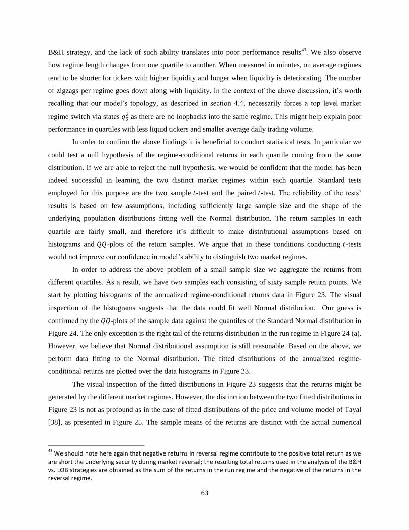
63

B&H strategy, and the lack of such ability translates into poor performance results43

. We also observe

how regime length changes from one quartile to another. When measured in minutes, on average regimes

tend to be shorter for tickers with higher liquidity and longer when liquidity is deteriorating. The number

of zigzags per regime goes down along with liquidity. In the context of the above discussion, it’s worth

recalling that our model’s topology, as described in section 4.4, necessarily forces a top level market

regime switch via states as there are no loopbacks into the same regime. This might help explain poor

performance in quartiles with less liquid tickers and smaller average daily trading volume.

In order to confirm the above findings it is beneficial to conduct statistical tests. In particular we

could test a null hypothesis of the regime-conditional returns in each quartile coming from the same

distribution. If we are able to reject the null hypothesis, we would be confident that the model has been

indeed successful in learning the two distinct market regimes within each quartile. Standard tests

employed for this purpose are the two sample -test and the paired -test. The reliability of the tests’

results is based on few assumptions, including sufficiently large sample size and the shape of the

underlying population distributions fitting well the Normal distribution. The return samples in each

quartile are fairly small, and therefore it’s difficult to make distributional assumptions based on

histograms and -plots of the return samples. We argue that in these conditions conducting -tests

would not improve our confidence in model’s ability to distinguish two market regimes.

In order to address the above problem of a small sample size we aggregate the returns from

different quartiles. As a result, we have two samples each consisting of sixty sample return points. We

start by plotting histograms of the annualized regime-conditional returns data in Figure 23. The visual

inspection of the histograms suggests that the data could fit well Normal distribution. Our guess is

confirmed by the -plots of the sample data against the quantiles of the Standard Normal distribution in

Figure 24. The only exception is the right tail of the returns distribution in the run regime in Figure 24 (a).

However, we believe that Normal distributional assumption is still reasonable. Based on the above, we

perform data fitting to the Normal distribution. The fitted distributions of the annualized regime-

conditional returns are plotted over the data histograms in Figure 23.

The visual inspection of the fitted distributions in Figure 23 suggests that the returns might be

generated by the different market regimes. However, the distinction between the two fitted distributions in

Figure 23 is not as profound as in the case of fitted distributions of the price and volume model of Tayal

[38], as presented in Figure 25. The sample means of the returns are distinct with the actual numerical

43

We should note here again that negative returns in reversal regime contribute to the positive total return as we are short the underlying security during market reversal; the resulting total returns used in the analysis of the B&H vs. LOB strategies are obtained as the sum of the returns in the run regime and the negative of the returns in the reversal regime.

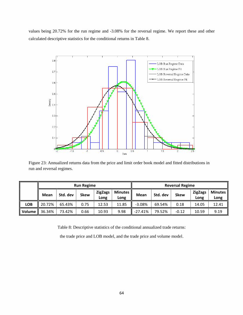
64

values being 20.72% for the run regime and -3.08% for the reversal regime. We report these and other

calculated descriptive statistics for the conditional returns in Table 8.

Figure 23: Annualized returns data from the price and limit order book model and fitted distributions in

run and reversal regimes.

Run Regime Reversal Regime

Mean Std. dev Skew ZigZags

Long Minutes

Long Mean Std. dev Skew

ZigZags Long

Minutes Long

LOB 20.72% 65.43% 0.75 12.53 11.85 -3.08% 69.54% 0.18 14.05 12.41

Volume 36.34% 73.42% 0.66 10.93 9.98 -27.41% 79.52% -0.12 10.59 9.19

Table 8: Descriptive statistics of the conditional annualized trade returns:

the trade price and LOB model, and the trade price and volume model.

65

(a)

(b)

Figure 24: (a) The -plot of the annualized returns in the run regime vs. quantiles of the Standard

Normal distribution; (b) the -plot of the annualized returns in the reversal regime vs. quantiles of the

Standard Normal distribution.

66

Figure 25: The annualized returns data from the price and volume model and the fitted distributions in the

run and reversal regimes.

In order to establish statistical significance of the difference between the two regimes we shall

employ the two-sample location -test, more commonly known as the Student’s -test44

. The initial

condition of the equal sample size is automatically satisfied as we have return statistics for each ticker in

both regimes. As already discussed, the validity of the test is based on several assumptions. The first

assumption is regarding the normality of the distributions from which the samples are drawn; as

mentioned earlier we believe this assumption is satisfied based on the -plots in Figure 24. The second

assumption for the test is related to the variances of the distributions from which the samples are drawn.

They are required to be the same. Although a formal statistical test can be performed to test for variance

equality, we believe that this assumption is satisfied, as we have sufficiently large samples and the

samples’ standard deviations are reasonably close, 65.43% for the run and 69.54% for the reversal

regimes45

.

44

There are multiple tests that could be conducted to establish statistical significance of results. Tayal [38] is using a one-sample t-test for each of the regimes in order to establish positivity of returns in the bullish regime and negativity of returns in the bearish regime; we would argue that separate tests might not be necessary. As long as the sample returns can be attributed to distributions with different means and there is a clear evidence against hypothesis in the two-sample t-test, the trading strategy would be to go “long” over bullish regimes, and “short” over bearish ones, regardless of whether returns are positive or negative. 45

Daly et al [7] suggest using a factor of three as a rule of thumb for variance equality verification. In our case the factor is slightly over one.

67

Our test is set up as the following:

The appropriate test statistic is

where and are the sample means and,

are the sizes of the respective

samples; and

is the pooled estimator for the common variance, which is

constructed using the sample variances and

. The test is conducted on the annualized returns in the

different market regimes as identified by the price and LOB model; the same test is conducted on the

annualized returns produced by the price and volume model for reference purposes. A 5% confidence

level is used in both cases. Test results are presented in Table 9.

Price and LOB Price and Volume

Not rejected Rejected

p-value 0.0602 0.0000

Confidence Interval

[-0.0104, 0.4863] [0.3509, 0.9242]

t-statistic 1.8981 4.4083

Table 9: The results of a two-sample t-test conducted at 5% significance level on annualized returns data

from price and LOB and price and volume models.

68

Price and LOB Price and Volume

Not rejected Rejected

p-value 0.0793 0.003

Confidence Interval

[-0.0287, 0.5046] [0.3048, 0.9703]

t-statistic 1.7870 3.8402

Table 10: The results of a paired -test conducted at 5% significance level on annualized returns data from

price and LOB and price and volume models.

The results of the test suggest that returns generated in the different market regimes by the price

and LOB model come from the same distribution; effectively, this means that the price and LOB model

has failed to distinguish the hidden regimes in a statistically significant way46

. On the other hand, the test

results of the returns generated by the price and volume model confirm earlier findings by Tayal [38] –

the distinct market regimes have been successfully identified by that model.

In order to improve our confidence in the results of the two-sample -test, we conduct a paired

two sample -test. This test has a greater statistical power than the unpaired test, and comes naturally in

our study, as each annualized return sample point in the run regime has a counterpart in the reversal

regime per ticker. The test setup is as following

and the appropriate test statistic is

where is the meanof the paired differences; is zero; is the sample variance of the differences in

the annualized returns; is the number of pairs; . The test results are presented in Table 10;

they confirm the findings of the two-sample -test.

46

One fact that speaks in favour of the price and LOB model is that the -test was marginally close to rejection of the null hypothesis with the -value being 0.0602 (the cutoff point for the 5% significance level is 0.05).

69

Conclusions

This study is motivated by the contradiction between the Efficient Market Hypothesis, widely accepted in

the academic literature, and the stunning performance consistently demonstrated by some asset

management firms. Our view is that if the price development process is not a random walk as the EMH

suggests, then one should be able to identify regimes in the market when either a bullish or a bearish

sentiment prevails. We further argue that despite the longer term trends, temporary changes in the price

direction due to local volatility exist.

Keeping all of the above in mind, we develop a suitable model. A Hierarchical Hidden Markov

Model of Tayal [38] is adapted for the purpose of this study. After conducting a thorough literature

research, we decide to study the properties of the Limit Order Book in search of the reliable information

for the generation of a trading signal. As a result, the order book imbalance is chosen as a representative

measure of the LOB’s state for the trend-support purposes. We use a time series of the price trend

supported by the order book imbalance as the observation feature for the model.

A comprehensive data set of transactions from the Toronto Stock Exchange is obtained. The data

is validated and cleaned. We build the Limit Order Book analyzer tool which is used to generate the

feature vectors for the sixty largest companies by the market capitalization during the studied time period.

We have twenty-two days of market data.

We use a five day rolling window to learn the model’s parameters. The resulting learned model is

used for the inference purposes with the sole goal of predicting the future hidden market states out of the

sample. The model produces a string of the predicted hidden states which are used to generate two sets of

70

annualized returns from a simple trading strategy. Based on these set of annualized returns, we study two

problems of interest.

First, we compare the total returns to the benchmark returns. We choose a simple daily buy and

hold trading strategy as our benchmark: a security is bought at the start of the trading, and sold with the

closing bell; both transactions happen at the prevailing market prices and yield daily returns. Second, we

establish whether our model is successful in learning two distinct market regimes. For this purpose we

compare the returns in the run regime and the reversal regime. We study the above problems in the

context of liquidity. We assess how liquidity of the underlying ticker affects the predictive ability of our

model and the profitability of the trading strategy. We divide our sample of annualized returns into four

groups based on the average daily trading volume of the underlying ticker.

Our analysis reveals that the trading strategy based on the price and LOB model performs well in

quartiles with high liquidity of the underlying tickers: the model has an edge and beats the simple daily

buy and hold strategy. The same conclusion is made for the model’s ability to distinguish the run and

reversal market regimes: we observe consistently higher returns in the run regime and lower returns

during the reversals for the two most liquid quartiles. Our model fails at both tasks in the illiquid

quartiles.

In order to establish statistical significance of our observations regarding the model’s ability to

distinguish the run and reversal market regimes we conduct two statistical tests. Due to the sample size

limitations the tests are performed on the aggregated samples of annualized returns. First, a two-sample -

test is conducted on the sample returns obtained in the different regimes. If the null hypothesis of the test

were rejected, we could argue that returns come from different distributions, and therefore our model is

able to identify the bullish and bearish market regimes. The two return samples used are sufficiently large,

and approximately normally distributed; variance of two samples is comparable. All of the above gives us

confidence in the test results. Unfortunately, at the 5% significance level we are unable to reject the

hypothesis about the samples being drawn from the same distribution. In order to confirm the results we

have conducted a paired -test; we are able to conduct the paired test as each ticker in the index has two

mean return estimates associated with it, one per regime. The results of this test are similar to those of the

first one.

The overall conclusion that we make is that the LOB model is capable of performing well and is

able to distinguish the run and reversal market regimes in high liquidity environments. It is most likely

that the model can be further developed, both in the feature selection and topology in order to improve the

71

overall performance. In this regard, the results of Tayal [38] that are validated in our tests serve as a great

inspiration for future research.

The topology of the model used in the current study is derived based on our subjective

understanding of the underlying phenomenon. It is however possible to algorithmically produce an HMM

by means of structural learning. A simple approach of learning all possible structures might be non-

tractable due to the number of structures exponentially growing with the number of nodes, and even

undesirable due to the issues with over-fitting. A score-based method of learning structure [16] applied to

a set of candidates could yield an improved topology.

The EM algorithm used in our study for the parameter estimation is that of a classic Baum-Welch

form proposed by Baum et al [2]. It is used to compute the maximum likelihood estimates without

additional weighting on the sample input data. Some previous studies ([15], [42]) used Exponentially

Weighted EM (EWEM) algorithm, in which recent observations are given more significant weight for

parameter estimation purposes. It remains unclear whether such a modification would be beneficial in the

framework of our model; however Idvall et al [15] show that EWEM did not significantly improve their

results.

Another possible direction for the future research is modification of the feature vector. In the

current study we have discretized the observation space, which consists of 18 simple events. We strongly

believe that such representation is, on one hand, sufficient to make a realistic model, and, on the other

hand, parsimonious enough not to drag the learning process into the realm of parameter estimation

difficulties and over-fitting. However, there are other possible configurations described in the literature.

Idvall et al [15], who studied foreign exchange high frequency data, suggest a model with a continuous

observation space - they used Gaussian Mixture Model for this purpose. Zhang [42] uses continuous

observation probability distribution function for the training stage, and switches to discrete distribution

function for prediction. However, there are several pitfalls related to the modeling of continuous

observations that one should be aware of. An assumption about distribution has to be made. The most

typical choice is a Gaussian Mixture Model, which can be easy to work with, but it does not necessarily

describe phenomena with the desired level of accuracy. Parameter estimation is another potential

difficulty.

Based on the results of the price and volume model of Tayal [38], the feature vector could be

modified to include the price as well as both volume and order book information. We intend to further

research the interaction of the volume and order book information as preliminary results on the combined

model show no significant improvement over the stand-alone models.

72

References

1. Austin, M., Bates, G., Dempster, M.A.H., Leemans, V., Williams S.N. Adaptive Systems for

foreign exchange trading. Quantitative Finance, Volume 4 (August 2004), C37-C45.

2. Baum, L., Petrie, T., Soules, G., Weiss N. A Maximization Technique Occurring in the Statistical

Analysis of Probabilistic Functions of Markov Chains. The Annals of Mathematical Statistics,

Vol. 41, No. 1 (Feb., 1970), pp. 164-171

3. http://www.bloomberg.com/apps/news?pid=nw&pname=mm_0108_story1.html

4. Cao, C., Hansch , O., Wang, X. Order Placement Strategies in a Pure Limit Order Book Market,

Journal of Financial Research, Vol. XXXI, 2008, 113-140

5. Chen Z., Forsyth, P.A. Implications of a regime switching model on natural gas storage valuation

and optimal operation. Quantitative Finance, 10:159-176, 2009.

6. Cont, R., Stoikov, S., Talreja, R. A stochastic model for order book dynamics. Operations

Research, Vol. 58, No. 3, May-June 2010, pp. 217-224

7. Daly, F., Hand, D.J., Jones, M.C., Lunn, A.D., McConway, K.J. Elements of Statistics. The Open

University, Prentice Hall, 1995.

8. Dempster, A.P., Laird, N.M., Rubin, D.B. Maximum Likelihood from Incomplete Data via the

EM Algorithm. Journal of the Royal Statistical Society. Series B (Methodological) 39 (1): 1–38,

1977.

9. http://en.wikipedia.org/wiki/Dark_liquidity

10. http://en.wikipedia.org/wiki/Markov_property

11. Fama, E. Efficient Capital Markets: A Review of Theory and Empirical Work. Journal of Finance

25 (2): 383–417.

12. Feng, Y., Yu, R. Stone, P. Two Stock-Trading Agents: Market Making and Technical Analysis.

Proc of AMECV Workshop, Springer LNAI, pp. 18-36, 2004.

13. Fine, S., Singer, Y. The Hierarchical Hidden Markov Model: Analysis and Applications. Machine

Learning, pages 41–62, 1998.

73

14. Granger, C.W. J., Morgenstern, O. Spectral Analysis of New York Stock Market Prices. Kyklos

16 (1): 1–27.

15. Idvall, P., Jonsson, C. Algorithmic Trading - Hidden Markov Models on Foreign Exchange Data.

Master’s Thesis. Linkoping, Sweden, 2008.

16. Jensen, F.V., Nielsen, T.D. Bayesian Networks and Decision Graphs. Springer, 2007.

17. Juang, B.J. Maximum likelihood estimation for mixture multivariate stochastic observations of

Markov chains. AT&T Technical Journal, 64(6): 1235-1249, 1985.

18. Juang, B.H., Levinson, S.E., Sondhi, M.M. Maximum likelihood estimation for multivariate

mixture observations of Markov chains. IEEE Transactions on Information Theory 32(2): 307-

1986.

19. Juang, B.H., Rabiner, L. Mixture autoregressive Markov hidden models for speech signals. IEEE

Transactions on Acoustics, Speech and Signal Processing. 33 (6): 1404-1413, 1985.

20. Kakade, S. M., Kearns, M., Mansour, Y., Ortiz, L.E. Competitive Algorithms for VWAP and

Limit Order Trading. EC '04 Proceedings of the 5th ACM Conference on Electronic Commerce,

2004.

21. Kearns, M., Ortiz, L. The Penn-Lehman automated trading project. IEEE Intelligent Systems, vol.

18, no. 6, pp. 22-31, Nov./Dec. 2003.

22. Liporace, L.A. Maximum likelihood estimation for multivariate observations of Markov sources.

IEEE Transactions on Information Theory, 28 (5): 729-734, 1982.

23. Lo, A., Mamaysky, H., Wang, J. Foundations of Technical Analysis: Computational Algorithms,

Statistical Inference, and Empirical Implementation. The Journal of Finance. Vol. LV, No. 4,

August 2004.

24. McCulloch, R.E., Tsay, R.S. Nonlinearity in High-Frequency Financial Data and Hierarchical

Models. Studies in Nonlinear Dynamics & Econometrics, Volume 5, Issue 1, 2001.

25. Montgomery, A.L., Zarnowitz, V., Tsay, R.S., Tiao, G.C. Forecasting the U.S. Unemployment

Rate, Journal of the American Statistical Association, 93: 478-493, 1998.

26. Murphy, K.P. Dynamic Bayesian Networks: Representation, Inference and Learning. Ph.D.

Thesis, University of California, Berkley, 2002.

27. Ord, Tim. The secret science of price and volume, Wiley 2008.

28. Poritz, A. Linear predictive Markov models and the speech signal. IEEE International Conference

on Acoustics, Speech, and Signal Processing: 1291-1294.

29. Rabiner, L.R. A tutorial on Markov models and selected applications in Speech Recognition.

Proceedings of the IEEE, 77 (2) : 257-286, 1989.

30. Rice, J. Mathematical Statistics and Data Analysis (Second ed.), Duxbury Press, 1995.

74

31. Saad, E.; Prokhorov, D.; and Wunsch, D. Comparative Study of Stock Trend Prediction Using

Time Delay, Recurrent and Probabilistic Neural Networks. IEEE Transactions on Neural

Networks 9 (6): 1456–1470.

32. Samuelson, P. Proof That Properly Anticipated Prices Fluctuate Randomly. Industrial

Management Review 6: 41–49, 1965.

33. Saunders, D. Robust Estimation and Portfolio Optimization. University of Waterloo, 2009

34. http://www.sec.gov/answers/orderbd.htm

35. Silaghi, G. C., Robu, V. An Agent Strategy for Automated Stock Market Trading Combining

Price and Order Book Information. Congress on Computational Intelligence Methods and

Applications, 2005 ICSC.

36. Slanina, F. Mean-field approximation for a limit order driven market. Phys. Rev., 64:056136,

2001.

37. Soros, G. The Alchemy of Finance. Simon & Schuster, 1988.

38. Tayal, A. Regime Switching and Technical Trading with Dynamic Bayesian Networks in High-

Frequency Stock Markets. Master’s Thesis, University of Waterloo, Waterloo, Ontario. 2009

39. http://www.tmx.com/en/trading/products_services/iceberg_orders.html

40. Trader Workstation User’s Guide. Interactive Brokers, 2009

41. Tsay, R.S. “Analysis of Financial Time Series”, Wiley & Sons, 2010.

42. Zhang, Y. Prediction of Financial Time Series with Hidden Markov Models. Master’s Thesis.

SFU, 2004

43. Ziemba, R; Ziemba W. Scenarios for Risk Management and Global Investment Strategies. The

Wiley Finance Series, 2008.

44. Zovko, I.I., Farmer, J.D. The power of patience: A behavioral regularity in limit order placement.

Quantitative Finance, 2(5):387–392, 2002.