Hierarchical GeneralizedLinear Models

in Practice

Roger Payne

VSN International, 5 The Waterhouse,Waterhouse Street, Hemel Hempstead, UKand Rothamsted Research, Harpenden, UK

email: Roger.Payne@vsni.co.uk

RSS Statistical Computing Section, 3rd April 2008

HGLMs – introduction

• Hierarchical generalized linear models• extend generalized linear models to >1 source of error

• include generalized linear mixed models as a special case• but the additional random terms are not constrained to follow a

Normal distribution, nor to have an identity link

• allow for modelling of the dispersion of the error terms• extending quasi-likelihood methods of Nelder & Pregibon (1987)

• have an efficient fitting algorithm• no numerical integration is required

• are explained in the book Generalized Linear Models with Random Effects: Unified Analysis via H-likelihood by Lee, Nelder & Pawitan (2006)

• examples available in GenStat for Windows 9th Edition onwards

• Hierarchical generalized nonlinear models• include nonlinear parameters in the HGLM fixed model

• in GenStat for Windows 10th Edition

..

HGLMs – definition

• expected value E(y) = μ

link η = g(μ)

distribution – Normal, Binomial, Poisson or Gamma (from exponential family)

• but linear predictor η = X β + ∑i Zi νi

now contains additional vectors of random effects νi with Normal, beta, gamma or inverse gamma distributions and with their own link functions

• Normal-identity gives a GLMM but HGLM algorithms use much improved Laplace approximations in their use of adjusted profile likelihood

• inference by h-likelihood

..

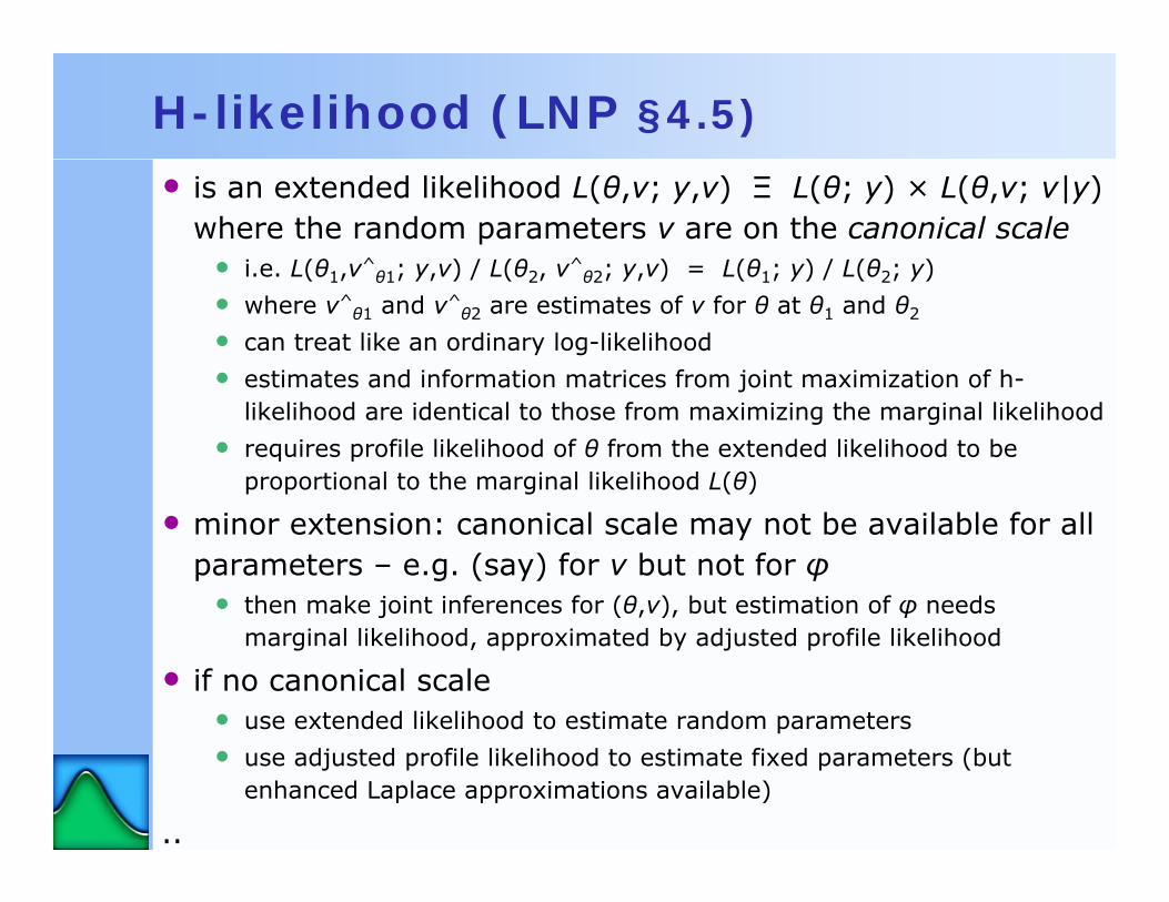
H-likelihood (LNP §4.5)

• is an extended likelihood L(θ,ν; y,ν) Ξ L(θ; y) × L(θ,ν; ν|y)where the random parameters v are on the canonical scale

• i.e. L(θ1,ν^θ1; y,ν) / L(θ2, ν^

θ2; y,ν) = L(θ1; y) / L(θ2; y)

• where ν^θ1 and ν^

θ2 are estimates of v for θ at θ1 and θ2

• can treat like an ordinary log-likelihood

• estimates and information matrices from joint maximization of h-likelihood are identical to those from maximizing the marginal likelihood

• requires profile likelihood of θ from the extended likelihood to be proportional to the marginal likelihood L(θ)

• minor extension: canonical scale may not be available for all parameters – e.g. (say) for v but not for φ

• then make joint inferences for (θ,v), but estimation of φ needs marginal likelihood, approximated by adjusted profile likelihood

• if no canonical scale• use extended likelihood to estimate random parameters

• use adjusted profile likelihood to estimate fixed parameters (but enhanced Laplace approximations available)

..

E.g. Normal-Normal HGLM• y = X β + Z ν + ε

• ε follows multivariate Normal(0,Σ), ν follows multivariate Normal(0,D)

• Σ and D parameterized by variance-component parameters τ=(σ2,σv2)

• so (LNP Example 6.1) we have linear predictor• η = g(μ) = X β + Z ν

• where g() is the identity function, and u=v

• and GLMs• y|u follows a GLM distribution with

• E(y|u) = μ

• var(y|u) = φV(μ) where φ=σ2, V(μ)=1

• u is distributed as Normal(0, λ), with λ=σv2

• constraint is E(u)=0

• extended likelihood (LNP §5.4) is• log L(θ,ν; y,ν) = log f(y,ν) = log f(y|ν) + log f(ν)

= ½log|2πΣ| – ½(y–Xβ–Zν)tΣ–1(y–Xβ–Zν) – ½log|2πD| – νtD–1ν

..

E.g. Normal-Normal HGLM• extended likelihood (LNP §5.4)

• log L(θ,ν; y,ν) = log f(y,ν) = log f(y|ν) + log f(ν)

= ½log|2πΣ| – ½(y–Xβ–Zν)tΣ–1(y–Xβ–Zν) – ½log|2πD| – νtD–1ν

• note: τ = (σ2,σv2) appears only in Σ and D

• Fisher information• I(v^) = ZtΣ–1Z + D–1

• depends on τ but not on β

• so scale v is canonical for β (but not for τ, which must be estimated by a marginal likelihood)

• i.e. the extended likelihood is an h-likelihood• joint estimation is possible for β and v

• but dispersion parameters τ estimated by adjusted profile likelihood

..

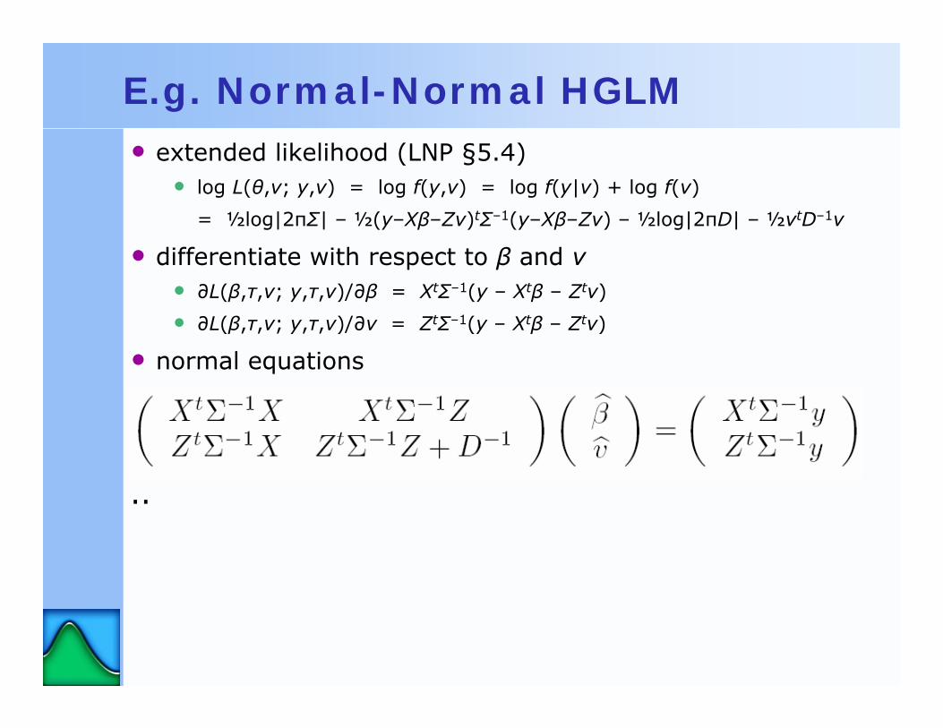
E.g. Normal-Normal HGLM• extended likelihood (LNP §5.4)

• log L(θ,ν; y,ν) = log f(y,ν) = log f(y|ν) + log f(ν)

= ½log|2πΣ| – ½(y–Xβ–Zν)tΣ–1(y–Xβ–Zν) – ½log|2πD| – ½νtD–1ν

• differentiate with respect to β and v• ∂L(β,τ,ν; y,τ,ν)/∂β = XtΣ–1(y – Xtβ – Ztν)

• ∂L(β,τ,ν; y,τ,ν)/∂v = ZtΣ–1(y – Xtβ – Ztν)

• normal equations

..

Augmented mean model• normal equations

• same equations are given by an augmented mean model

• ΨM Ξ E(u) = 0

• write as ya = Tδ + ε*

• normal equations are (TtΣa–1T)–1 δ^ = TtΣa

–1y (as above)

• can fit as an ordinary weighted regression

• see LNP §5.3.5

..

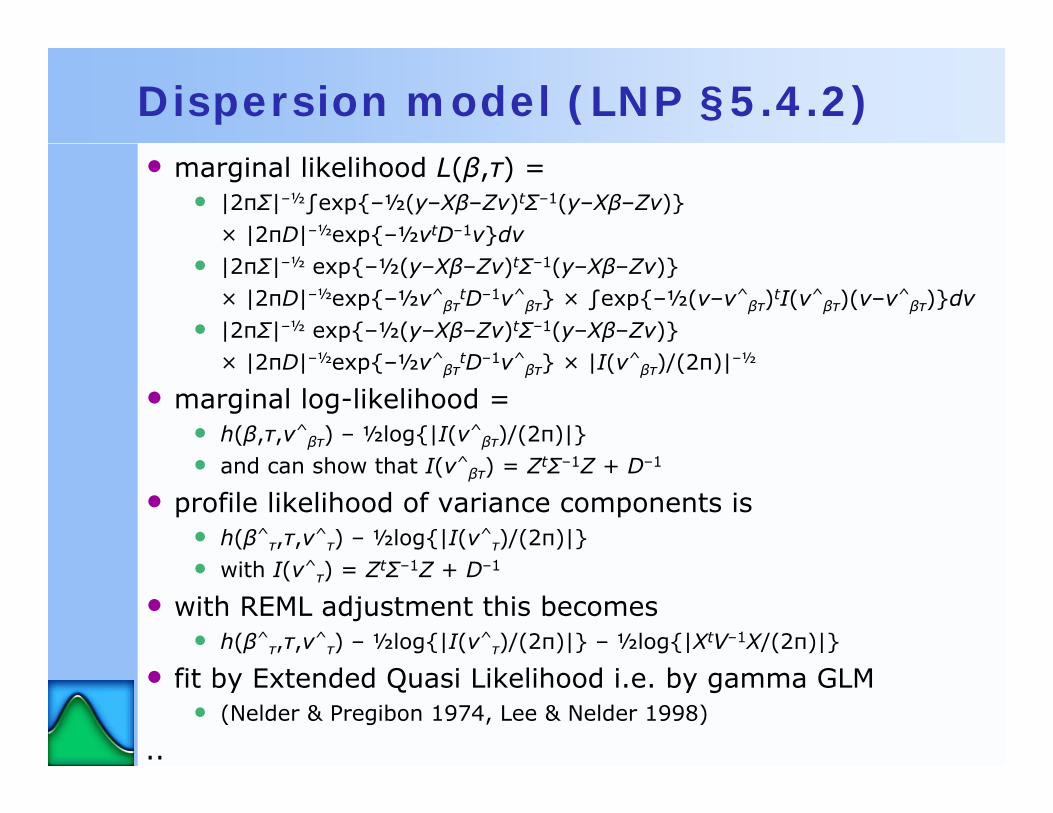
Dispersion model (LNP §5.4.2)• marginal likelihood L(β,τ) =

• |2πΣ|–½∫exp{–½(y–Xβ–Zν)tΣ–1(y–Xβ–Zν)}× |2πD|–½exp{–½νtD–1ν}dν

• |2πΣ|–½ exp{–½(y–Xβ–Zν)tΣ–1(y–Xβ–Zν)}× |2πD|–½exp{–½ν^

βτtD–1ν^

βτ} × ∫exp{–½(ν–ν^βτ)tI(ν^

βτ)(ν–ν^βτ)}dν

• |2πΣ|–½ exp{–½(y–Xβ–Zν)tΣ–1(y–Xβ–Zν)}× |2πD|–½exp{–½ν^

βτtD–1ν^

βτ} × |I(ν^βτ)/(2π)|–½

• marginal log-likelihood =• h(β,τ,ν^

βτ) – ½log{|I(ν^βτ)/(2π)|}

• and can show that I(ν^βτ) = ZtΣ–1Z + D–1

• profile likelihood of variance components is• h(β^

τ,τ,ν^τ) – ½log{|I(ν^

τ)/(2π)|}• with I(ν^

τ) = ZtΣ–1Z + D–1

• with REML adjustment this becomes• h(β^

τ,τ,ν^τ) – ½log{|I(ν^

τ)/(2π)|} – ½log{|XtV–1X/(2π)|}

• fit by Extended Quasi Likelihood i.e. by gamma GLM• (Nelder & Pregibon 1974, Lee & Nelder 1998)

..

Fitting algorithm

• interconnected Normal and Gamma GLMs (§5.4.4)

HGLMs in GenStat

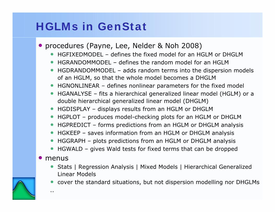
• procedures (Payne, Lee, Nelder & Noh 2008)• HGFIXEDMODEL – defines the fixed model for an HGLM or DHGLM• HGRANDOMMODEL – defines the random model for an HGLM• HGDRANDOMMODEL – adds random terms into the dispersion models

of an HGLM, so that the whole model becomes a DHGLM• HGNONLINEAR – defines nonlinear parameters for the fixed model• HGANALYSE – fits a hierarchical generalized linear model (HGLM) or a

double hierarchical generalized linear model (DHGLM)• HGDISPLAY – displays results from an HGLM or DHGLM• HGPLOT – produces model-checking plots for an HGLM or DHGLM• HGPREDICT – forms predictions from an HGLM or DHGLM analysis• HGKEEP – saves information from an HGLM or DHGLM analysis• HGGRAPH – plots predictions from an HGLM or DHGLM analysis• HGWALD – gives Wald tests for fixed terms that can be dropped

• menus• Stats | Regression Analysis | Mixed Models | Hierarchical Generalized

Linear Models• cover the standard situations, but not dispersion modelling nor DHGLMs..

GenStat HGLM examples

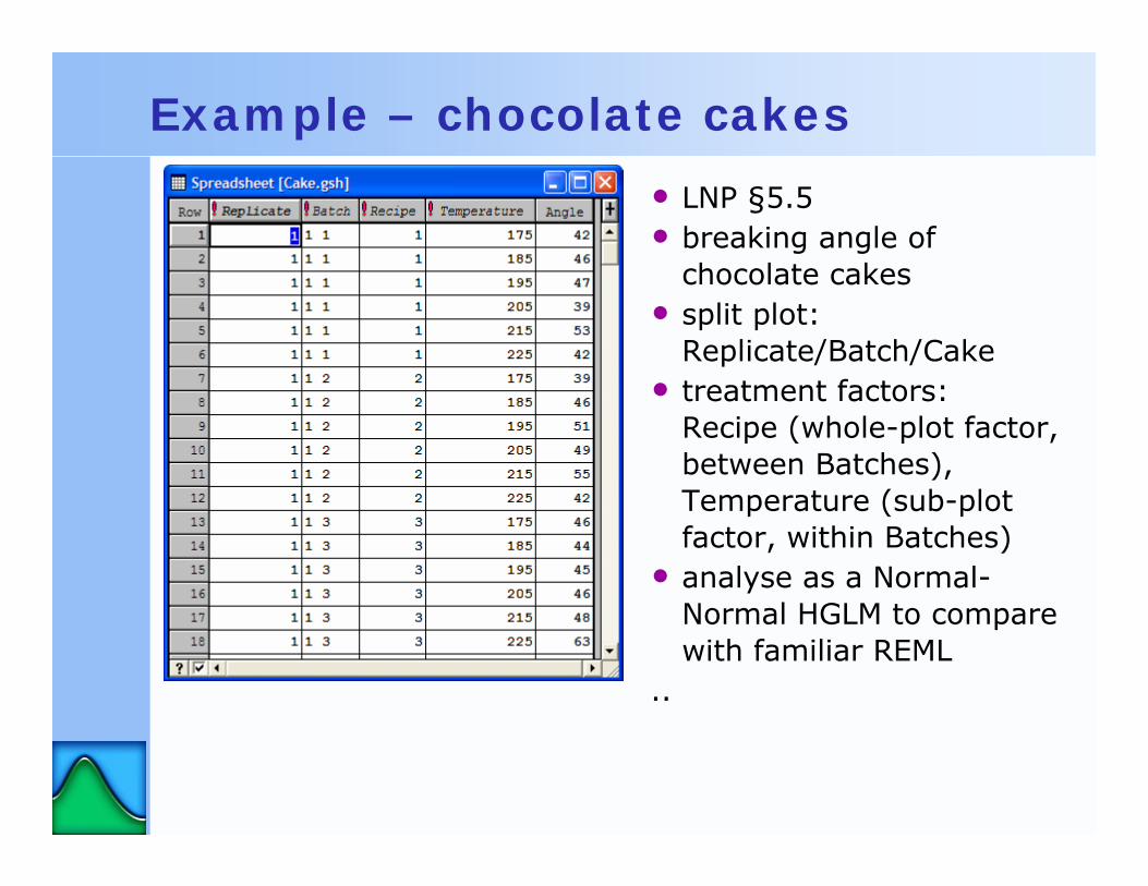
Example – chocolate cakes

• LNP §5.5• breaking angle of

chocolate cakes• split plot:

Replicate/Batch/Cake• treatment factors:

Recipe (whole-plot factor, between Batches), Temperature (sub-plot factor, within Batches)

• analyse as a Normal-Normal HGLM to compare with familiar REML

..

HGLM menu – for cakes

• find menu in Mixed models section of Regression Analysis on Stats menu

Output: Normal-Normal HGLM

mean model

dispersion model here just fits variance components

estimates of parameters in the mean model

..

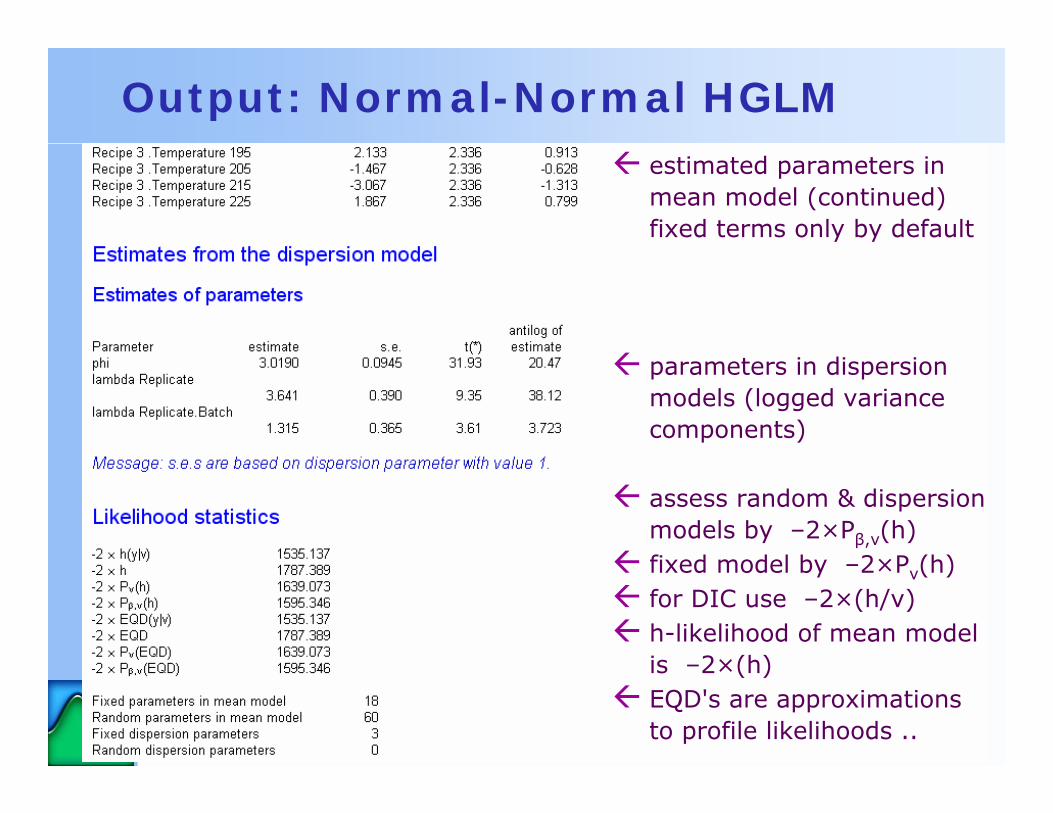
Output: Normal-Normal HGLMestimated parameters in mean model (continued) fixed terms only by default

parameters in dispersion models (logged variance components)

assess random & dispersion models by –2×Pβ,v(h)fixed model by –2×Pv(h)for DIC use –2×(h/v)h-likelihood of mean model is –2×(h)EQD's are approximations to profile likelihoods ..

Further output and model checking

• click on Further Output button in HGLM menu

• click on Model Checking button in HGLM Further Outputmenu to obtain HGLM Model Checking menu

..

Residual plots for cakes

Residual plots for batches

Residual plots for replicates

Residual plots for dispersion model

Compare to REML

Assess fixed model using –2 pν(h)

Assess fixed model using –2 pν(h)

Conjugate HGLMs• random parameters are on the canonical scale

• the contribution of the random parameters to the extended likelihood (Ξ the h-likelihood) has the same form as the likelihood of the base GLM

• so it can easily be fitted together with the base GLM in the augmented mean model (same variance function, same iterative reweighting scheme etc...)

• examples• Normal – Normal most obvious

• Poisson – Gamma most useful?

• Binomial – Beta next most useful?

• Gamma – Inverse Gamma

• algorithmically and intuitively appealing

..

Conjugate HGLM e.g. Poisson-Gamma • Poisson-gamma HGLM (LNP Ex. 6.2 & 6.3): linear predictor

•η = log(μ) = X β + Z ν

•where v = log(u)

• Poisson-gamma HGLM: distributions•y|u follows a Poisson distribution with E(y|u) = μ

• log-likelihood is ∑{ y log(μ) – μ }

•u has a Gamma distribution

• log-likelihood is ∑{(ψM log(u) – u – log(λ)/λ – logΓ(1/λ)}

• ψM = E(u) = 1

• this is the conjugate distribution for the Poisson (so this is a conjugate HGLM)

• note: gamma distribution for random effects has VM(u) = u and log canonical link, but standard gamma GLM has V(μ) = μ2 and reciprocal canonical link

• kernel of h-loglikelihood (LNP §6.3) is•∑{ y log(μ) – μ } + ∑{(ψM log(u) – u – log(λ)/λ – logΓ(1/λ)}

•v is canonical for β (but not λ)

•estimate λ by profile lhd (c.f. variance components in normal-normal)

..

Non-conjugate HGLMs• random parameters no longer on the canonical scale

• use extended likelihood to estimate random parameters

• use adjusted profile likelihood to estimate fixed parameters

• but enhanced Laplace approximations available (Noh & Lee 06)

• augmented mean model now has a different GLM for the base GLM from the augmented units

• examples

• Poisson – Normal Poisson GLMM

• Binomial – Normal Binomial GLMM

• Gamma – Normal Gamma GLMM

• algorithmically more difficult, but can still be fitted within the GLM framework

..

HGLMs

• examples of HGLMs (LNP Table 6.2)

Birds in Tasmania• HGLM

• base GLM – Poisson distribution, Log link

• random terms – Gamma distribution, Log link

• i.e. Poisson-Gamma conjugate HGLM

• random terms• site (Site)

• treatment locations within site (SiteTreat)

• sample plots within treatment locations (Plot)

• fixed terms• connected by habitat strips (Treatment)

• vegetation type (Vegetation)

• time of day (AM_vs_PM)

• data set used by Steve Candy, Forestry Tasmania, at the Workshop Extensions of Generalized Linear Models(Nelder, Payne & Candy) before the Australasian Genstat Conference, Surfers Paradise, 30 January 2001

..

Vegetation * Treatment * AM_vs_PM

mean model

dispersion model

likelihood statistics

d.f.

Wald tests

•no evidence of a 3-factor interaction

..

Omit Vegetation.Treatment.AM_vs_PM

Wald tests and Change

• change deviance 2.60 on 2 d.f. for omitting Vegetation.Treatment.AM_vs_PM (c.f. Wald 2.58)

• next omit Vegetation.Treatment

..

Omit Vegetation.Treatment

Wald tests and Change

• change deviance 4.42 on 2 d.f. for omitting Vegetation.Treatment (c.f. Wald 4.49)

• next omit Vegetation.AM_PM

..

Omit Vegetation.AM_PM

Wald tests and Change

• change deviance 4.97 on 2 d.f. for omitting Vegetation.AM_PM (c.f. Wald 5.00)

• now study results

..

Predicted means: treatment x time of day

Hierarchical generalized nonlinear models

• expected value E(y) = μ

link η = g(μ)

distribution – Normal, Binomial, Poisson or Gamma (from exponential family)

linear predictor η = X β + ∑i Zi γi

random effects γi with either beta, Normal, gamma or inverse gamma distributions, and their own link functions

• nonlinear parameters in fixed terms in the linear predictor

• X β = ∑ xi βi

• but now some xi's are nonlinear functions of explanatory variables and parameters that are to be estimated

• extension of generalized nonlinear models of Lane (1996)

• constraint – available only for conjugate HGLM's

..

Implementation – interlinked GLMs• fit nonlinear parameters by maximizing h-likelihood

of augmented mean model

• Hooded Parrot (Psephotus dissimilis)

• grass parrot in Northern Territory of Australia

• nests in termite mounds• nests also inhabited by

moth larvae that feed on nestling waste

Acknowledgement: S CooneyAustralian National University, Canberrahttp://www.anu.edu.au/BoZo/stuart/HPP.htm

Growth of Hooded Parrot nestlings

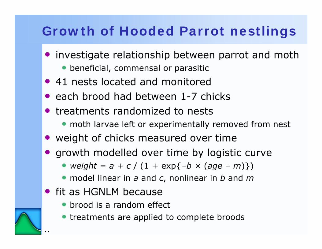
• investigate relationship between parrot and moth• beneficial, commensal or parasitic

• 41 nests located and monitored• each brood had between 1-7 chicks• treatments randomized to nests

• moth larvae left or experimentally removed from nest

• weight of chicks measured over time• growth modelled over time by logistic curve

• weight = a + c / (1 + exp{–b × (age – m)})• model linear in a and c, nonlinear in b and m

• fit as HGNLM because• brood is a random effect• treatments are applied to complete broods

..

Growth of Hooded Parrot nestlings

Initial values from logistic curve

HGNLM, common A, B, C and M

HGNLM, common A, B, C and M

HGNLM, common B, C and M

HGNLM, common B, C and M

HGNLM, common B and M

HGNLM, common B and M

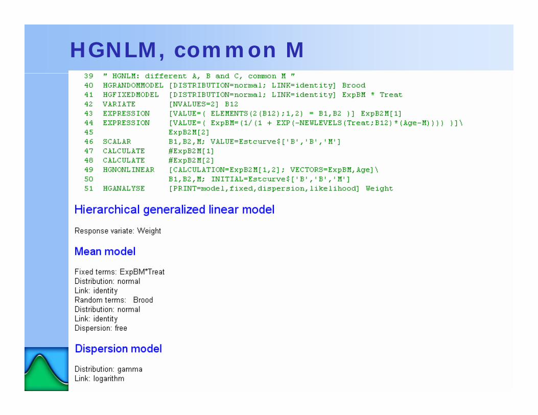
HGNLM, common M

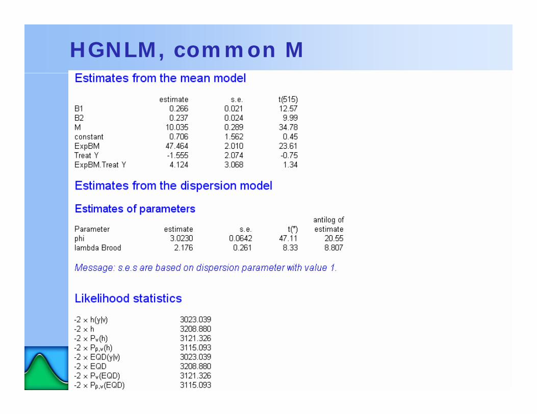
HGNLM, common M

HGNLM, different A, B, C and M

HGNLM, different A, B, C and M

Likelihood statistics

•no evidence of any treatment effects

..

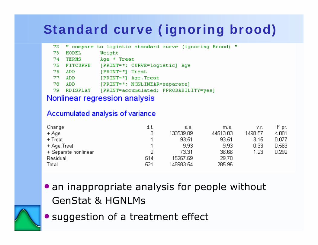
Standard curve (ignoring brood)

•an inappropriate analysis for people without GenStat & HGNLMs

• suggestion of a treatment effect

GNLM with Brood as a fixed term

•an alternative inappropriate analysis

• significant (but misleading) treatment effects

Conclusions

• the HGLM menus & procedures provide very useful extensions to the standard Generalized linear Models

• represent the current state of the ongoing research by Lee, Nelder et al. on extensions to generalized linear models

• GenStat is providing a flexible and convenient framework for the collaboration – to try out, and then distribute, our ideas

• the methodology is described in the book• Lee, Y., Nelder, J.A. & Pawitan, Y. (2006). Generalized Linear Models

with Random Effects: Unified Analysis via H-likelihood. CRC Press.

• there are many extensions (+ corrections) since then• including HGNLMs, in GenStat for Windows 10th Edition

• Wald tests and plots of predicted means to come in the 11th Edition

• for further information, see vsni.co.uk or email roger.payne@vsni.co.uk

..