Hierarchical Forecasting · Hierarchical Forecasting approaches rather than single level approaches...

ISSN 1440-771X

Department of Econometrics and Business Statistics

http://business.monash.edu/econometrics-and-business-statistics/research/publications

February 2019

Working Paper 02/19

Hierarchical Forecasting

George Athanasopoulos, Puwasala Gamakumara, Anastasios Panagiotelis, Rob J Hyndman and

Mohamed Affan




George AthanasopoulosDepartment of Econometrics and Business Statistics,Monash University,VIC 3800, Australia.Email: [email protected]

Puwasala GamakumaraDepartment of Econometrics and Business Statistics,Monash University,VIC 3800, Australia.Email: [email protected]

Anastasios PanagiotelisDepartment of Econometrics and Business Statistics,Monash University,VIC 3800, Australia.Email: [email protected]

Rob J HyndmanDepartment of Econometrics and Business Statistics,Monash University,VIC 3800, Australia.Email: [email protected]

Mohamed AffanEmail: [email protected]

14 February 2019

JEL classification: ??


Abstract

Accurate forecasts of macroeconomic variables are crucial inputs into the decisions of economic

agents and policy makers. Exploiting inherent aggregation structures of such variables, we

apply forecast reconciliation methods to generate forecasts that are coherent with the aggre-

gation constraints. We generate both point and probabilistic forecasts for the first time in the

macroeconomic setting. Using Australian GDP we show that forecast reconciliation not only

returns coherent forecasts but also improves the overall forecast accuracy in both point and

probabilistic frameworks.

1 Introduction

Accurate forecasting of key macroeconomic variables such as Gross Domestic Product (GDP),

inflation, and industrial production, has been at the forefront of economic research over many

decades. Early approaches involved univariate models or at best low dimensional multivariate

systems. The era of big data has led to the use of regularization and shrinkage methods

such as dynamic factor models, Lasso, LARS, and Bayesian VARs, in an effort to exploit the

plethora of potentially useful predictors now available. These predictors commonly also include

the components of the variables of interest. For instance, GDP is formed as an aggregate

of consumption, government expenditure, investment and net exports, with each of these

components also formed as aggregates of other economic variables. While the macroeconomic

forecasting literature regularly uses such sub-indices as predictors, it does so in ways that

fail to exploit accounting identities that describe known deterministic relationships between

macroeconomic variables.

In this paper we take a different approach. Over the past decade there has been a growing

literature on forecasting collections of time series that follow aggregation constraints, known

as hierarchical time series. Initially the aim of this literature was to ensure that forecasts

adhered to aggregation constraints thus ensuring aligned decision making. However in many

empirical settings the forecast reconciliation methods designed to deal with this problem have

also been shown to improve forecast accuracy. Examples include forecasting accidents and

emergency admissions (Athanasopoulos et al., 2017), mortality rates (Shang and Hyndman,

2017), prison populations (Athanasopoulos, Steel, and Weatherburn, 2019), retail sales (Villegas

and Pedregal, 2018), solar energy (Yang et al., 2017; Yagli, Yang, and Srinivasan, 2019), tourism

demand (Athanasopoulos, Ahmed, and Hyndman, 2009; Hyndman et al., 2011; Wickramasuriya,

2


Athanasopoulos, and Hyndman, 2018), and wind power generation (Zhang and Dong, 2019).

Both aligned decision making and forecast accuracy are key concerns for economic agents and

policy makers. To the best of our knowledge the only application of forecast reconciliation

methods to macroeconomics focuses on point forecasting for inflation (Capistrán, Constandse,

and Ramos-Francia, 2010; Weiss, 2018). In this paper we illustrate the application of state-of-the-

art forecast reconciliation methods to macroeconomic forecasting in point as well as probabilistic

frameworks.

The remainder of the paper is set out as follows. Section 2 introduces the concept of hierarchical

time series, i.e. collections of time series with known linear constraints, with a particular

emphasis on macroeconomic examples. Section 3 describes state-of-the-art forecast reconciliation

techniques for point forecasts, while Section 4 describes the more recent extension of these

techniques to probabilistic forecasting. Section 5 describes the data used in our empirical case

study, namely Australian GDP data, represented using two alternative hierarchical structures.

Section 6 provides details on the setup of our empirical study including criteria used for the

evaluation of both point and probabilistic forecasts. Section 7 presents results and Section 8

concludes providing future avenues for research that are of particular relevance to the empirical

macroeconomist.

2 Hierarchical time series

To simplify the introduction of the notation we use the simple two-level hierarchical structure

shown in Figure 1. Let yTot,t denote the value observed at time t for the most aggregate (Total)

series corresponding to level 0 of the hierarchy. Below level 0, denote as yi,t the value of the

series corresponding to node i, observed at time t. For example, yA,t denotes the tth observation

of the series corresponding to node A at level 1, yAB,t denotes the tth observation of the series

corresponding to node AB at level 2, and so on.

Total

A

AA AB

B

BA BB BC

Figure 1: A simple two-level hierarchical structure.

Let yt = (yTot,t, yA,t, yB,t, yAA,t, yAB,t, yBA,t, yBB,t, yBC,t)′ denote a vector containing observations

across all series of the hierarchy at time t. Similarly denote as bt = (yAA,t, yAB,t, yBA,t, yBB,t, yBC,t)′

Athanasopoulos, Gamakumara, Panagiotelis, Hyndman, & Affan: February 14, 2019 3


a vector containing observations only for the bottom-level series. In general, yt ∈ Rn and

bt ∈ Rm where n denotes the number of total series in the structure, m the number of series at

the bottom level, and n > m always. In the simple example of Figure 1, n = 8 and m = 5.

Aggregation constraints dictate that yTot = yA,t + yB,t = yAA,t + yAB,t + yBA,t + yBB,t +

yBC,t, yA,t = yAA,t + yAB,t and yB = yBA,t + yBB,t + yBC,t. Hence we can write

yt = Sbt,

where

S =

1 1 1 1 1

1 1 0 0 0

0 0 1 1 1

I5

is an n × m matrix referred to as the summing matrix and Im is an m-dimensional identity

matrix. S reflects the linear aggregation constraints and in particular how the bottom-level series

aggregate to levels above. Thus, columns of S span the linear subspace of Rn for which the

aggregation constraints hold. We refer to this as the coherent subspace and denote it by s. Notice

that pre-multiplying a vector in Rm by S will result in an n-dimensional vector that lies in s.

Property 2.1 A hierarchical time series has observations that are coherent, i.e., yt ∈ s for all t. We use

the term coherent to describe not just yt but any vector in s.

Structures similar to the one shown in Figure 1 can be found in macroeconomics. For instance,

in Section 5 we consider two alternative hierarchical structures for the case of GDP and its

components. However, while this motivating example involves aggregation constraints, the

mathematical framework we use can be applied for any general linear constraints, examples

of which are ubiquitous in macroeconomics. For instance, the trade balance is computed as

exports minus imports, while the consumer price index is computed as a weighted average of

sub-indices, which are in turn weighted averages of sub-sub-indices, and so on. These structures

can also be captured by an appropriately designed S matrix.

An important alternative aggregation structure, also commonly found in macroeconomics, is

one for which the most aggregate series is disaggregated by attributes of interest that are crossed,

as distinct to nested which is the case for hierarchical time series. For example, industrial

production may be disaggregated along the lines of geography or sector or both. We refer to

this as a grouped structure. Figure 2 shows a simple example of such a structure. The Total



series disaggregates into yA,t and yB,t, but also into yX,t and yY,t, at level 1, and then into the

bottom-level series, bt = (yAX, yAY, yBX, yBY)′. Hence, in contrast to hierarchical structures,

grouped time series do not naturally disaggregate in a unique manner.

AX AY A

BX BY B

X Y Total

Figure 2: A simple two-level grouped structure.

An important implementation of aggregation structures are temporal hierarchies introduced by

Athanasopoulos et al. (2017). In this case the aggregation structure spans the time dimension

and dictates how higher frequency data (e.g., monthly) are aggregated to lower frequencies (e.g.

quarterly, annual). There is a vast literature that studies the effects of temporal aggregation,

going back to the seminal work of Zellner and Montmarquette (1971), Amemiya and Wu (1972),

Tiao (1972), and Brewer (1973) and others, including Hotta (1993), Hotta and Cardoso Neto

(1993), Marcellino (1999), and Silvestrini et al. (2008). The main aim of this work is to find the

single best level of aggregation for modelling and forecasting time series. In this literature, the

analyses, results (whether theoretical or empirical) and inferences, are extremely heterogeneous,

making it very challenging to reach a consensus or to draw firm conclusions. For example,

Rossana and Seater (1995) who study the effect of aggregation on several key macroeconomic

variables state:

“Quarterly data do not seem to suffer badly from temporal aggregation distortion,

nor are they subject to the construction problems affecting monthly data. They

therefore may be the optimal data for econometric analysis.”

A similar conclusion is reached by Nijman and Palm (1990). Silvestrini et al. (2008) consider fore-

casting French cash state deficit and provide empirical evidence of forecast accuracy gains from

forecasting with the aggregate model rather than aggregating forecasts from the disaggregate

model.

The vast majority of this literature concentrates on a single level of temporal aggregation

(although there are some notable exceptions such as Andrawis, Atiya, and El-Shishiny, 2011;

Kourentzes, Petropoulos, and Trapero, 2014). Athanasopoulos et al. (2017) show that considering

multiple levels of aggregation via temporal hierarchies and implementing forecast reconciliation



approaches rather than single level approaches results in substantial gains in forecast accuracy

across all levels of temporal aggregation.

3 Point forecasting

A requirement when forecasting hierarchical time series is that the forecasts adhere to the same

aggregation constraints as the observed data; i.e., they are coherent.

Definition 3.1 A set of h-step-ahead forecasts yT+h|T, stacked in the same order as yt and generated

using information up to and including time T, are said to be coherent if yT+h|T ∈ s.

Hence, coherent forecasts of lower level series aggregate to their corresponding upper level

series and vice versa.

Let us consider the smallest possible hierarchy with two bottom-level series, depicted in Figure 3,

where yTot = yA + yB. While base forecasts could lie anywhere in R3, the realisations and

coherent forecasts lie in a two dimensional subspace s ⊂ R3.

3.1 Single-level approaches

A common theme across all traditional approaches for forecasting hierarchical time series is that

a single-level of aggregation is first selected and forecasts for that level are generated. These are

then linearly combined to generate a set of coherent forecasts in the rest of the structure.

3.1.1 Bottom-up

In the bottom-up approach, forecasts for the most disaggregate level are first generated. These

are then aggregated to obtain forecasts for all other series of the hierarchy (Dunn, Williams,

and Dechaine, 1976). In general, this consists of first generating bT+h|T ∈ Rm, a set of h-step-

ahead forecasts for the bottom-level series. For the simple hierarchical structure of Figure 1,

bT+h|T = (yAA,T+h|T, yAB,T+h|T, yBA,T+h|T, yBB,T+h|T, yBC,T+h|T), where yi,T+h|T is the h-step-ahead

forecast of the series corresponding to node i. A set of coherent forecasts for the whole hierarchy

is then given by

yBUT+h|T = SbT+h|T.

Generating bottom-up forecasts has the advantage of no information being lost due to aggrega-

tion. However, bottom-level data can potentially be highly volatile or very noisy and therefore

challenging to forecast.



3.1.2 Top-down

In contrast, top-down approaches involve first generating forecasts for the most aggregate level

and then disaggregating these down the hierarchy. In general, coherent forecasts generated

from top-down approaches are given by

yTDT+h|T = SpyTot,T+h|T,

0.0 0.2 0.4 0.6 0.8 1.0

0.0

0.5

1.0

1.5

2.0

0.0

0.2

0.4

0.6

0.8

1.0

yA

y B

y Tot s1

s2

s

Figure 3: Representation of a coherent subspace in a three dimensional hierarchy where yTot = yA + yB.The coherent subspace is depicted as a gray two dimensional plane labelled s. Note that thecolumns of~s1 = (1, 1, 0)′ and~s2 = (1, 0, 1)′ form a basis for s. The red points lying on s canbe either realisations or coherent forecasts.



where p = (p1, . . . , pm)′ is an m-dimensional vector consisting of a set of proportions that

disaggregate the top-level forecast yTot,T+h|T to forecasts for the bottom-level series; hence

pyTot,T+h|T = bT+h|T. These are then aggregated up by the summing matrix S.

Traditionally, proportions have been calculated based on the observed historical data. Gross

and Sohl (1990) present and evaluate twenty-one alternative approaches. The most convenient

attribute of these approaches is their simplicity. Generating a set of coherent forecasts involves

modelling and generating forecasts only for the most aggregate top-level series. In general,

such top-down approaches seem to produce quite reliable forecasts for the aggregate levels

and they are useful with low count data. However, a significant disadvantage is the loss of

information due to aggregation. A limitation of such top-down approaches is that characteristics

of lower level series cannot be captured. To overcome this, Athanasopoulos, Ahmed, and

Hyndman (2009) introduced a new top-down approach which disaggregates the top-level

based on proportions of forecasts rather than the historical data and showed that this method

outperforms the conventional top-down approaches. However, a limitation of all top-down

approaches is that they introduce bias to the forecasts even when the top-level forecast itself is

unbiased. We discuss this in detail in Section 3.2.

3.1.3 Middle-out

A compromise between bottom-up and top-down approaches is the middle-out approach. It

entails first forecasting the series of a selected middle-level. For series above the middle-level,

coherent forecasts are generated using the bottom-up approach by aggregating the middle-level

forecasts. For series below the middle level, coherent forecasts are generated using a top-down

approach by disaggregating the middle-level forecasts. Since the middle-out approach involves

generating top-down forecasts, it also introduces bias to the forecasts.

3.2 Point forecast reconciliation

All approaches discussed so far are limited to only using information from a single-level

of aggregation. Furthermore, these ignore any correlations across levels of a hierarchy. An

alternative framework that overcomes these limitations is one that involves forecast reconciliation.

In a first step. forecasts for all the series across all levels of the hierarchy are computed, ignoring

any aggregation constraints. We refer to these as base forecasts and denote them by yT+h|T. In

general, base forecasts will not be coherent, unless a very simple method has been used to

compute them such as for naïve forecasts. In this case, forecasts are simply equal to a previous

realisation of the data and they inherit the property of coherence.



The second step is an adjustment that reconciles base forecasts so that they become coherent. In

general, this is achieved by mapping the base forecasts yT+h|T onto the coherent subspace s via

a matrix SG, resulting in a set of coherent forecasts yT+h|T. Specifically,

yT+h|T = SGyT+h|T, (1)

where G is an m× n matrix that maps yT+h|T to Rm, producing new forecasts for the bottom

level, which are in turn mapped to the coherent subspace by the summing matrix S. We restrict

our attention to projections on s in which case SGS = S. This ensures that unbiasedness is

preserved, i.e., for a set of unbiased base forecasts reconciled forecasts will also be unbiased.

Note that all single-level approaches discussed so far can also be represented by (1) using

appropriately designed G matrices, however not all of these will be projections. For example

for the bottom-up approach, G =(

0(m×n−m) Im

)in which case SGS = S. For any top-down

approach G =(

p 0(m×n−1)

), for which SGS 6= S.

3.2.1 Optimal MinT reconciliation

Wickramasuriya, Athanasopoulos, and Hyndman (2018) build a unifying framework for much

of the previous literature on forecast reconciliation. We present here a detailed outline of this

approach and in turn relate it to previous significant contributions in forecast reconciliation.

Assume that yT+h|T is a set of unbiased base forecasts, i.e., E1:T(yT+h|T) = E1:T[yT+h | y1, . . . , yT],

the true mean with the expectation taken over the observed sample up to time T. Let

eT+h|T = yT+h|T − yT+h|T (2)

denote a set of base forecast errors with Var(eT+h|T) = Wh, and

eT+h|T = yT+h|T − yT+h|T

denote a set of coherent forecast errors. Lemma 1 in Wickramasuriya, Athanasopoulos, and

Hyndman (2018) shows that for any matrix G such that SGS = S, Var(eT+h|T) = SGWhS′G′.

Furthermore Theorem 1 shows that

G = (S′W−1h S)−1S′W−1

h



is the unique solution that minimises the trace of SGWhS′G′ subject to SGS = S. MinT is

optimal in the sense that given a set of unbiased base forecasts, it returns a set of best linear

unbiased reconciled forecasts, using as G the unique solution that minimises the trace (hence

MinT) of the variance of the forecast error of the reconciled forecasts.

A significant advantage of the MinT reconciliation solution is that it is the first to incorporate

the full correlation structure of the hierarchy via Wh. However, estimating Wh is challenging,

especially for h > 1. Wickramasuriya, Athanasopoulos, and Hyndman (2018) present possible

alternative estimators for Wh and show that these lead to different G matrices. We summarise

these below.

• Set Wh = kh In for all h, where kh > 0 is a proportionality constant. This simple assump-

tion returns G = (S′S)−1S′ so that the base forecasts are orthogonally projected onto the

coherent subspace s minimising the Euclidean distance between yT+h|T and yT+h|T. Hynd-

man et al. (2011) come to same solution, however from the perspective of the following

regression model

yT+h|T = SβT+h|T + εT+h|T,

where βT+h|T = E[bT+h | b1, . . . , bT] is the unknown conditional mean of the bottom-level

series and εT+h|T is the coherence or reconciliation error with mean zero and variance

V . The OLS solution leads to the same projection matrix S(S′S)−1S′, and due to this

interpretation we continue to refer to this reconciliation method as OLS. A disadvantage

of the OLS solution is that the homoscedastic diagonal entries do not account for the scale

differences between the levels of the hierarchy due to aggregation. Furthermore, OLS does

not account for the correlations across series.

• Set Wh = khdiag(W1) for all h (kh > 0), where

W1 =1T

T

∑T=1

et e′t

is the unbiased sample estimator of the in-sample one-step-ahead base forecast errors

as defined in (2). Hence this estimator scales the base forecasts using the variance of

the in-sample residuals and is therefore described and referred to as a weighted least

squares (WLS) estimator applying variance scaling. A similar estimator was proposed by

Hyndman, Lee, and Wang (2016).

An alternative WLS estimator is proposed by Athanasopoulos et al. (2017) in the context

of temporal hierarchies. Here Wh is proportional to diag(S1) where 1 is a unit column



vector of dimension n. Hence the weights are proportional to the number of bottom-level

variables required to form an aggregate. For example, in the hierarchy of Figure 1, the

weights corresponding to the Total, series A and series B are proportional to 5, 2 and 3

respectively. This weighting scheme depends only on the aggregation structure and is

referred to as structural scaling. Its advantage over OLS is that it assumes equivariant

forecast errors only at the bottom level of the structure and not across all levels. It is

particularly useful in cases where forecast errors are not available; for example, in cases

where the base forecasts are generated by judgemental forecasting.

• Set Wh = khW1 for all h (kh > 0) to be proportional to the unrestricted sample covariance

estimator for h = 1. Although this is relatively simple to obtain and provides a good

solution for small hierarchies, it does not provide reliable results as m grows compared to

T. This is referred to this as the MinT(Sample) estimator.

• Set Wh = khW D1 for all h (kh > 0), where W D

1 = λDdiag(W1) + (1− λD)W1 is a shrinkage

estimator with diagonal target and shrinkage intensity parameter

λD =∑i 6=j Var(rij)

∑i 6=j r2ij

,

where rij is the (i, j)th element of R1, the one-step-ahead sample correlation matrix as

proposed by Schäfer and Strimmer (2005). Hence, off-diagonal elements of W1 are shrunk

towards zero while diagonal elements (variances) remain unchanged. This is referred to

as the MinT(Shrink) estimator.

4 Hierarchical probabilistic forecasting

A limitation of point forecasts is that they provide no indication of uncertainty around the

forecast. A richer description of forecast uncertainty can be obtained by providing a probabilistic

forecast, also commonly referred to as a density forecast. For a review of probabilistic forecasts,

and scoring rules for evaluating such forecasts, see (Gneiting and Katzfuss, 2014). In recent years,

the use of probabilistic forecasts and their evaluation via scoring rules has become pervasive

in macroeconomic forecasting, some notable (but non-exhaustive) examples are Geweke and

Amisano (2010), Billio et al. (2013), Carriero, Clark, and Marcellino (2015) and Clark and

Ravazzolo (2015).

The literature on hierarchical probabilistic forecasting is still an emerging area of interest. To the

best of our knowledge the first attempt to even define coherence in the setting of probabilistic



forecasting is provided by Taieb, Taylor, and Hyndman (2017) who define a coherent forecast

in terms of a convolution. An equivalent definition due to Gamakumara et al. (2018) defines a

coherent probabilistic forecast as a probability measure on the coherent subspace s. Gamakumara

et al. (2018) also generalise the concept of forecast reconciliation to the probabilistic setting.

Definition 4.1 Let A be a subset1 of s and let B be all points in Rn that are mapped onto A after

premultiplication by SG. Letting ν be a base probabilistic forecast for the full hierarchy, the coherent

measure ν reconciles ν if ν(A) = ν(B) for all A.

In practice this definition leads to two approaches. For some parametric distributions, for

instance the multivariate normal, a reconciled probabilistic forecast can be derived analyti-

cally. However, in macroeconomic forecasting, non-standard distributions such as bimodal

distributions are often required to take different policy regimes into account. In such cases a

non-parametric approach based on bootstrapping in-sample errors proposed Gamakumara et al.

(2018) can be used. These scenarios are now covered in detail.

4.1 Probabilistic forecast reconciliation in the Gaussian framework

In the case where the base forecasts are probabilistic forecasts characterised by elliptical dis-

tributions, Gamakumara et al. (2018) show that reconciled probabilistic forecasts will also be

elliptical. This is particularly straightforward for the Gaussian distribution which is completely

characterised by two moments. Letting the base probabilistic forecasts be N (yT+h|T, ΣT+h|T),

then the reconciled probabilistic forecasts will be N (yT+h|T, ΣT+h|T), where

yT+h|T = SGyT+h|T

and ΣT+h|T = SGΣT+h|TG′S′.

There are several options for obtaining the base probabilistic forecasts and in particular the

variance covariance matrix Σ. One option is to fit multivariate models either level by level or for

the hierarchy as a whole leading respectively to a Σ that is block diagonal or dense. Another

option is to fit univariate models for each individual series in which case Σ is a diagonal matrix.

A third option that we employ here is to obtain Σ using in-sample forecast errors, in a similar

vein to how W1 is estimated in the MinT method. Here the same shrinkage estimator described

in Section 3.2 is used. The reconciled probabilistic forecast will ultimately depend on the choice

of G; the same choices of G matrices used in Section 3 can be used.1Strictly speaking A is a Borel set



4.2 Probabilistic forecast reconciliation in the non-parametric framework

In many applications, including macroeconomic forecasting, it may not be reasonable to assume

Gaussian predictive distributions. Therefore, non-parametric approaches have been widely used

for probabilistic forecasts in different disciplines. For example, ensemble forecasting in weather

applications (Gneiting, 2005; Gneiting and Katzfuss, 2014; Gneiting et al., 2008), and bootstrap

based approaches (Manzan and Zerom, 2008; Vilar and Vilar, 2013). In macroeconomics, Cogley,

Morozov, and Sargent (2005) discuss the importance of allowing for skewness in density forecasts

and more recently Smith and Vahey (2016) discuss this issue in detail.

Due to these concerns, we employ the bootstrap method proposed by Gamakumara et al. (2018)

that does not make parametric assumptions about the predictive distribution. An important

result exploited by this method is that applying point forecast reconciliation to the draws from

an incoherent base predictive distribution, results in a sample from the reconciled predictive

distribution. We summarise this process below:

1. Fit univariate models to each series in the hierarchy over a training set from t = 1, . . . , T.

2. For each series compute h-step-ahead point forecasts, for h = 1, . . . , H. Collect these into

an n× H matrix Y := (yT+1|T, . . . , yT+H|T), where yT+h|T is an n-vector of h-step-ahead

point forecasts for all series in the hierarchy.

3. Compute one-step-ahead in-sample forecast errors. Collect these into an n× T matrix

E = (e1, e2, . . . , eT), where the n-vector et = yt − yt|t−1. Here, yt|t−1 is a vector of forecasts

made for time t using information up to and including time t− 1. These are called in-

sample forecasts since while they depend only on past values, information from the entire

training sample is used to estimate the parameters for the models on which the forecasts

are based.

4. Block bootstrap from E; that is choose H consecutive columns of E at random, repeating

this process B times. Denote the n× H matrix obtained at iteration b as Eb for b = 1, . . . , B.

5. For all b, compute Υb := Y + Eb. Each row of Υb is a sample path of h forecasts for a

single series. Each column of Υb is a realisation from the joint predictive distribution at a

particular horizon.

6. For each b = 1, . . . , B, select the hth column of Υb and stack these to form an n× B matrix

ΥT+h|T.



7. For a given G matrix and for each h = 1, . . . , H, compute ΥT+h|T = SGΥT+h|T. Each

column of ΥT+h|T is a realisation from the joint h-step-ahead reconciled predictive distribu-

tion.

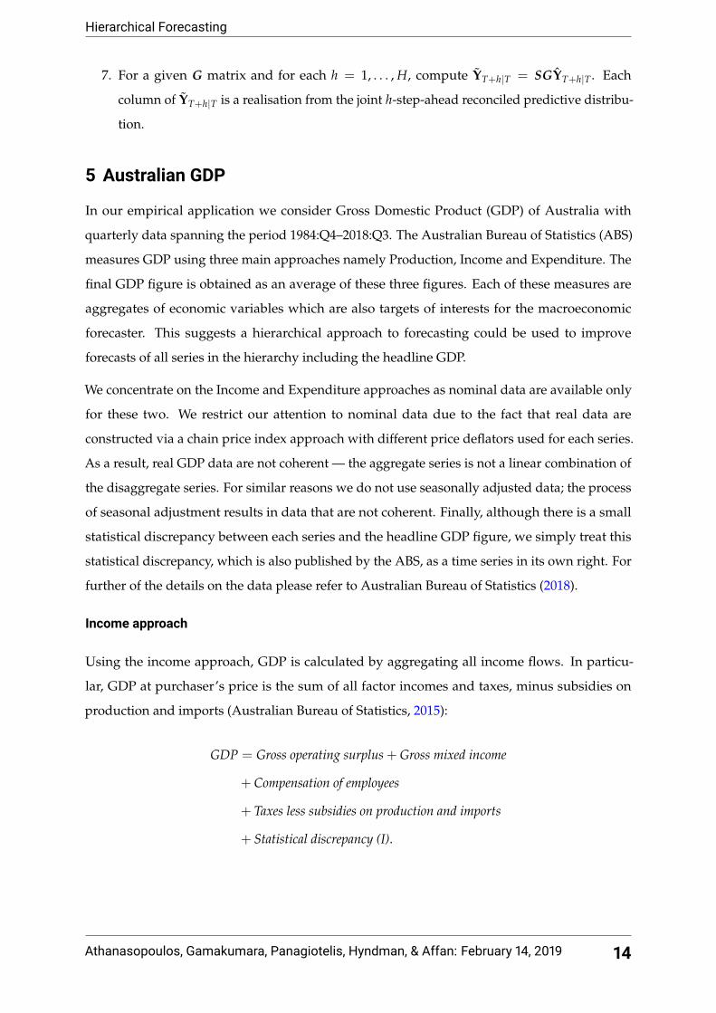
5 Australian GDP

In our empirical application we consider Gross Domestic Product (GDP) of Australia with

quarterly data spanning the period 1984:Q4–2018:Q3. The Australian Bureau of Statistics (ABS)

measures GDP using three main approaches namely Production, Income and Expenditure. The

final GDP figure is obtained as an average of these three figures. Each of these measures are

aggregates of economic variables which are also targets of interests for the macroeconomic

forecaster. This suggests a hierarchical approach to forecasting could be used to improve

forecasts of all series in the hierarchy including the headline GDP.

We concentrate on the Income and Expenditure approaches as nominal data are available only

for these two. We restrict our attention to nominal data due to the fact that real data are

constructed via a chain price index approach with different price deflators used for each series.

As a result, real GDP data are not coherent — the aggregate series is not a linear combination of

the disaggregate series. For similar reasons we do not use seasonally adjusted data; the process

of seasonal adjustment results in data that are not coherent. Finally, although there is a small

statistical discrepancy between each series and the headline GDP figure, we simply treat this

statistical discrepancy, which is also published by the ABS, as a time series in its own right. For

further of the details on the data please refer to Australian Bureau of Statistics (2018).

Income approach

Using the income approach, GDP is calculated by aggregating all income flows. In particu-

lar, GDP at purchaser’s price is the sum of all factor incomes and taxes, minus subsidies on

production and imports (Australian Bureau of Statistics, 2015):

GDP = Gross operating surplus + Gross mixed income

+ Compensation of employees

+ Taxes less subsidies on production and imports

+ Statistical discrepancy (I).



Figure 4 shows the full hierarchical structure capturing all components aggregated to form GDP

using the income approach. The hierarchy has two levels of aggregation below the top-level,

with a total of n = 16 series across the whole structure and m = 10 series at the bottom level.

Figure 4: Hierarchical structure of the income approach for GDP. The pink cell contains GDP the mostaggregate series. The blue cells contain intermediate-level series and the yellow cells correspondto the most disaggregate bottom-level series.

Expenditure approach

In the expenditure approach, GDP is calculated as the aggregation of final consumption ex-

penditure, gross fixed capital formation (GFCF), changes in inventories of finished goods,

work-in-progress and raw materials and the value of exports less imports of the goods and

services (Australian Bureau of Statistics, 2015). The underline equation is:

GDP = Final consumption expenditure + Gross fixed capital formation

+ Changes in inventories + Trade balance + Statistical discrepancy (E).

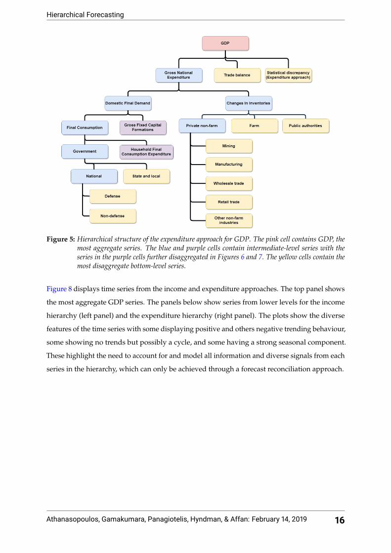
Figures 5, 6 and 7 show the full hierarchical structure capturing all components aggregated to

form GDP using the expenditure approach. The hierarchy has three levels of aggregation below

the top-level, with a total of n = 80 series across the whole structure and m = 53 series at the

bottom level. Descriptions of each series in these hierarchies along with the series ID assigned

by the ABS are given in the Tables 1, 2, 3 and 4 in the Appendix.



Figure 5: Hierarchical structure of the expenditure approach for GDP. The pink cell contains GDP, themost aggregate series. The blue and purple cells contain intermediate-level series with theseries in the purple cells further disaggregated in Figures 6 and 7. The yellow cells contain themost disaggregate bottom-level series.

Figure 8 displays time series from the income and expenditure approaches. The top panel shows

the most aggregate GDP series. The panels below show series from lower levels for the income

hierarchy (left panel) and the expenditure hierarchy (right panel). The plots show the diverse

features of the time series with some displaying positive and others negative trending behaviour,

some showing no trends but possibly a cycle, and some having a strong seasonal component.

These highlight the need to account for and model all information and diverse signals from each

series in the hierarchy, which can only be achieved through a forecast reconciliation approach.



Figure 6: Hierarchical structure for Gross Fixed Capital Formations under the expenditure approach forGDP, continued from Figure 5. Blue cells contain intermediate-level series and the yellow cellscorrespond to the most disaggregate bottom-level series.



Figure 7: Hierarchical structure for Household Final Consumption Expenditure under the expenditureapproach for GDP, continued from Figure 5. Blue cells contain intermediate-level series andthe yellow cells correspond to the most disaggregate bottom-level series.



100

200

300

400

1990 2000 2010

Time

$ bi

llion

s

GDP

TfiG

osCopN

fnT

fiGosC

opNfnP

ubS

di

1990 2000 2010

25

50

75

2

3

4

5

−4

−2

0

2

4

6

Time

$ bi

llion

s

Income

GneC

iiG

neDfdG

fcPvtP

biNdm

Sha

GneC

iiPba

1990 2000 2010

−3

0

3

6

−2

−1

0

−2

0

2

Time

$ bi

llion

s

Expenditure

Figure 8: Time plots for series from different levels of income and expenditure hierarchies.



6 Empirical application methodology

We now demonstrate the potential for reconciliation methods to improve forecast accuracy

for Australian GDP. We consider forecasts from h = 1 quarter ahead up to h = 4 quarters

ahead using an expanding window. First, the training sample is set from 1984:Q4 to 1994:Q3

and forecasts are produced for 1994:Q4 to 1995:Q3. Then the training window is expanded

by one quarter at a time, i.e. from 1984:Q4 to 2017:Q4 with the final forecasts produced for

the last available observation in 2018:Q1. This leads to 94 1-step-ahead, 93 2-steps-ahead, 92

3-steps-ahead and 91 4-steps-ahead forecasts available for evaluation.

6.1 Models

The first task in forecast reconciliation is to obtain base forecasts for all series in the hierarchy.

In the case of the income approach, this necessitates forecasting n = 16 separate time series

while in the case of the expenditure approach, forecasts for n = 80 separate time series must

be obtained. Given the diversity in these time series discussed in Section 5, we focus on an

approach that is fast but also flexible. We consider simple univariate ARIMA models, where

model order is selected via a combination of unit root testing and the AIC using an algorithm

developed by Hyndman and Khandakar (2008) and implemented in the auto.arima() function

in Hyndman et al. (2019). A similar approach was also undertaken using the ETS framework to

produce base forecasts (Hyndman et al., 2008). This had minimal impact on our conclusions with

respect to forecast reconciliation methods, and in most cases ARIMA forecasts were found to be

more accurate than ETS forecasts. Consequently for brevity, we have excluded presenting the

results for ETS models. However, these are available from github 2 and are discussed in detail in

Gamakumara, 2019. We note that a number of more complicated approaches could have been

used to obtain base forecasts including multivariate models such as vector autoregressions, and

models and methods that handle a large number of predictors such as factor models or least

angle regression. However, Panagiotelis et al. (2019) show that univariate ARIMA models are

highly competitive for forecasting Australian GDP even compared to these methods, and in any

case our primary motivation is to demonstrate the potential of forecast reconciliation.

The hierarchical forecasting approaches we consider are bottom-up, OLS, WLS with variance

scaling and the MinT(Shrink) approach. The MinT(Sample) approach was also used but due

to the size of the hierarchy, forecasts reconciled via this approach were less stable. Finally, all

forecasts (both base and coherent) are compared to a seasonal naïve benchmark (Hyndman and

Athanasopoulos, 2018); i.e. the forecast for GDP (or one of its components) is the realised GDP

2The relevant github repository is PuwasalaG/Hierarchical-Book-Chapter


https://github.com/PuwasalaG/Hierarchical-Book-Chapter


in the same quarter of the previous year. The naïve forecasts are by construction coherent and

therefore do not need to be reconciled.

6.2 Evaluation

For evaluating point forecasts we consider two metrics, the Mean Squared Error (MSE) and

the Mean Absolute Scaled Error (MASE) calculated over the expanding window. The absolute

scaled error is defined as

qT+h =|eT+h|T|

(T − 4)−1 ∑Tt=5 |yt − yt−4|

,

where et+h is the difference between any forecast and the realisation3, and 4 is used due to the

quarterly nature of the data. An advantage of using MASE is that it is a scale independent

measure. This is particularly relevant for hierarchical time series, since aggregate series by

their very nature are on a larger scale than disaggregate series. Consequently, scale dependent

metrics may unfairly favour methods that perform well for the aggregate series but poorly for

disaggregate series. For more details on different point forecast accuracy measures, refer to

Chapter 3 of Hyndman and Athanasopoulos (2018).

Forecast accuracy of probabilistic forecasts can be evaluated using scoring rules (Gneiting and

Katzfuss, 2014). Let F be a probabilistic forecast and let y ∼ F where a breve is again used

to denote that either base forecasts or coherent forecasts can be evaluated. The accuracy of

multivariate probabilistic forecasts will be measured by the energy score given by

eS(FT+h|T, yT+h) = EF‖yT+h − yT+h‖α − 12

EF‖yT+h − y∗T+h‖α ,

where yT+h is the realisation at time T + h, and α ∈ (0, 2]. We set α = 1, noting that other values

of α give similar results. The expectations can be evaluated numerically as long as a sample from

F is available, which is the case for all methods we employ. An advantage of using energy scores

is that in the univariate case it simplifies to the commonly used cumulative rank probability

score (CRPS) given by

CRPS(Fi, yi,T+h) = EFi|yi,T+h − yi,T+h| −

12

EFi|yi,T+h − y∗i,T+h|,

where the subscript i is used to denote that CRPS measures forecast accuracy for a single variable

in the hierarchy.

3Breve is used instead of a hat or tilde to denote that this can be the error for either a base or reconciled forecast.



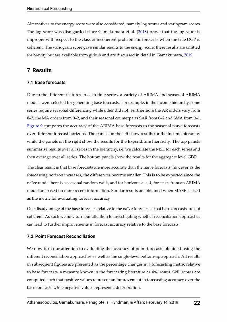
Alternatives to the energy score were also considered, namely log scores and variogram scores.

The log score was disregarded since Gamakumara et al. (2018) prove that the log score is

improper with respect to the class of incoherent probabilistic forecasts when the true DGP is

coherent. The variogram score gave similar results to the energy score; these results are omitted

for brevity but are available from github and are discussed in detail in Gamakumara, 2019

7 Results

7.1 Base forecasts

Due to the different features in each time series, a variety of ARIMA and seasonal ARIMA

models were selected for generating base forecasts. For example, in the income hierarchy, some

series require seasonal differencing while other did not. Furthermore the AR orders vary from

0–3, the MA orders from 0–2, and their seasonal counterparts SAR from 0–2 and SMA from 0–1.

Figure 9 compares the accuracy of the ARIMA base forecasts to the seasonal naïve forecasts

over different forecast horizons. The panels on the left show results for the Income hierarchy

while the panels on the right show the results for the Expenditure hierarchy. The top panels

summarise results over all series in the hierarchy, i.e. we calculate the MSE for each series and

then average over all series. The bottom panels show the results for the aggregate level GDP.

The clear result is that base forecasts are more accurate than the naïve forecasts, however as the

forecasting horizon increases, the differences become smaller. This is to be expected since the

naïve model here is a seasonal random walk, and for horizons h < 4, forecasts from an ARIMA

model are based on more recent information. Similar results are obtained when MASE is used

as the metric for evaluating forecast accuracy.

One disadvantage of the base forecasts relative to the naïve forecasts is that base forecasts are not

coherent. As such we now turn our attention to investigating whether reconciliation approaches

can lead to further improvements in forecast accuracy relative to the base forecasts.

7.2 Point Forecast Reconciliation

We now turn our attention to evaluating the accuracy of point forecasts obtained using the

different reconciliation approaches as well as the single-level bottom-up approach. All results

in subsequent figures are presented as the percentage changes in a forecasting metric relative

to base forecasts, a measure known in the forecasting literature as skill scores. Skill scores are

computed such that positive values represent an improvement in forecasting accuracy over the

base forecasts while negative values represent a deterioration.



4.0e+06

8.0e+06

1.2e+07

1.6e+07

1 2 3 4

h

MS

E

All levels

2e+07

4e+07

6e+07

8e+07

1 2 3 4

h

MS

E

Top level

Income

1e+06

2e+06

3e+06

4e+06

1 2 3 4

h

MS

E

All levels

2e+07

4e+07

6e+07

8e+07

1 2 3 4

h

MS

E

Top level

Expenditure

Method Base Naive

Figure 9: Mean squared errors for naïve and ARIMA base forecasts. Top panels refer to results sum-marised over all series while bottom panels refer to results for the top-level GDP series. Leftpanels refer to the income hierarchy and right panels to the expenditure hierarchy.

Figures 10 and 11 show skill scores using MSE and MASE respectively. The top row of each figure

shows skill scores based on averages over all series. We conclude that reconciliation methods

generally improve forecast accuracy relative to base forecasts regardless of the hierarchy used,

the forecasting horizon, the forecast error measure or the reconciliation method employed. We do

however note that while all reconciliation methods improve forecast performance, MinT(Shrink)

is the best forecasting method in most cases.

To further investigate the results we break down the skill scores by different levels of each

hierarchy. The second row of Figures 10 and 11 shows the skill scores for a single series, namely

GDP which represents the top-level of both hierarchies. The third row shows results for all

series excluding those of the bottom level, while the final row shows results for the bottom-level

series only. Here, we see two general features. The first is that OLS reconciliation performs

poorly on the bottom-level series, and the second is that bottom-up performs relatively poorly

on aggregate series. The two features are particularly exacerbated for the larger expenditure

hierarchy. These results are consistent with other findings in the forecast reconciliation literature

(see for instance Athanasopoulos et al., 2017; Wickramasuriya, Athanasopoulos, and Hyndman,

2018)



0

3

6

9

1 2 3 4

h

All levels

−10

−5

0

5

10

1 2 3 4

h

Top level

0

5

10

1 2 3 4

h

Aggregate levels

−5.0

−2.5

0.0

2.5

5.0

1 2 3 4

h

Bottom level

Income

−20

−10

0

1 2 3 4

h

All levels

−40

−30

−20

−10

0

10

1 2 3 4

h

Top level

−30

−20

−10

0

10

1 2 3 4

h

Aggregate levels

−2.5

0.0

2.5

5.0

7.5

1 2 3 4

h

Bottom level

Expenditure

Method MinT(Shrink) WLS OLS Bottom−up

Ski

ll sc

ore

(MS

E)

%

Figure 10: Skill scores for point forecasts from alternative methods (with reference to base forecasts)using MSE. The left panels refer to the income hierarchy while the right panels refer to theexpenditure hierarchy. The first row refers to results summarised over all series, the secondrow to top-level GDP series, the third row to aggregate levels, and the last row to the bottomlevel.



−10

−5

0

1 2 3 4

h

All levels

−10

−5

0

1 2 3 4

h

Top level

0.0

2.5

5.0

1 2 3 4

h

Aggregate levels

−25

−20

−15

−10

−5

0

1 2 3 4

h

Bottom level

Income

−8

−4

0

1 2 3 4

h

All levels

−15

−10

−5

0

5

1 2 3 4

h

Top level

0

2

4

1 2 3 4

h

Aggregate levels

−15

−10

−5

0

1 2 3 4

h

Bottom level

Expenditure


Ski

ll sc

ore

(MA

SE

) %

Figure 11: Skill scores for point forecasts from different reconciliation methods (with reference to baseforecasts) using MASE. The left two panels refer to the income hierarchy and the right twopanels to the expenditure hierarchy. The first row refers to results summarised over all series,the second row to top-level GDP series, the third row to aggregate levels, and the last row tothe bottom level.



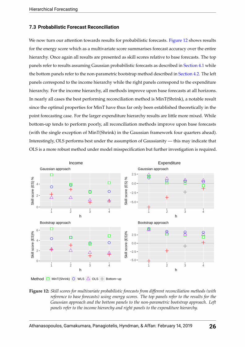
7.3 Probabilistic Forecast Reconciliation

We now turn our attention towards results for probabilistic forecasts. Figure 12 shows results

for the energy score which as a multivariate score summarises forecast accuracy over the entire

hierarchy. Once again all results are presented as skill scores relative to base forecasts. The top

panels refer to results assuming Gaussian probabilistic forecasts as described in Section 4.1 while

the bottom panels refer to the non-parametric bootstrap method described in Section 4.2. The left

panels correspond to the income hierarchy while the right panels correspond to the expenditure

hierarchy. For the income hierarchy, all methods improve upon base forecasts at all horizons.

In nearly all cases the best performing reconciliation method is MinT(Shrink), a notable result

since the optimal properties for MinT have thus far only been established theoretically in the

point forecasting case. For the larger expenditure hierarchy results are little more mixed. While

bottom-up tends to perform poorly, all reconciliation methods improve upon base forecasts

(with the single exception of MinT(Shrink) in the Gaussian framework four quarters ahead).

Interestingly, OLS performs best under the assumption of Gaussianity — this may indicate that

OLS is a more robust method under model misspecification but further investigation is required.

0

2

4

1 2 3 4

h

Ski

ll sc

ore

(ES

) %

Gaussian approach

0

2

4

6

1 2 3 4

h

Ski

ll sc

ore

(ES

)%

Bootstrap approach

Income

−5.0

−2.5

0.0

2.5

1 2 3 4

h

Ski

ll sc

ore

(ES

) %

Gaussian approach

−5.0

−2.5

0.0

2.5

1 2 3 4

h

Ski

ll sc

ore

(ES

)%

Bootstrap approach

Expenditure


Figure 12: Skill scores for multivariate probabilistic forecasts from different reconciliation methods (withreference to base forecasts) using energy scores. The top panels refer to the results for theGaussian approach and the bottom panels to the non-parametric bootstrap approach. Leftpanels refer to the income hierarchy and right panels to the expenditure hierarchy.



−7.5

−5.0

−2.5

0.0

2.5

1 2 3 4

h

Ski

ll sc

ore

(CR

PS

) %

Gaussian approach

−6

−3

0

3

1 2 3 4

h

Ski

ll sc

ore

(CR

PS

)%

Bootstrap approach

Income

−15

−10

−5

0

1 2 3 4

h

Ski

ll sc

ore

(CR

PS

) %

Gaussian approach

−15

−10

−5

0

5

1 2 3 4

h

Ski

ll sc

ore

(CR

PS

) %

Bootstrap approach

Expenditure


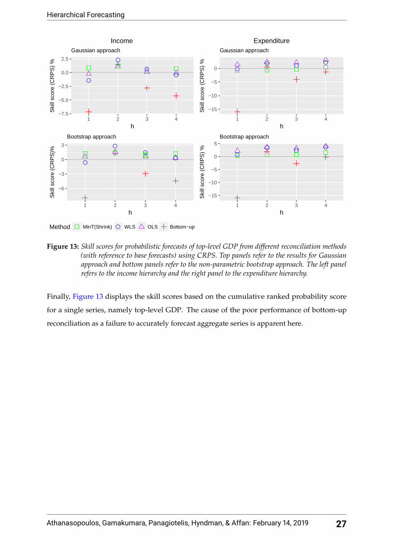
Figure 13: Skill scores for probabilistic forecasts of top-level GDP from different reconciliation methods(with reference to base forecasts) using CRPS. Top panels refer to the results for Gaussianapproach and bottom panels refer to the non-parametric bootstrap approach. The left panelrefers to the income hierarchy and the right panel to the expenditure hierarchy.

Finally, Figure 13 displays the skill scores based on the cumulative ranked probability score

for a single series, namely top-level GDP. The cause of the poor performance of bottom-up

reconciliation as a failure to accurately forecast aggregate series is apparent here.



8 Conclusions

In the macroeconomic setting, we have demonstrated the potential for forecast reconciliation

methods to not only provide coherent forecasts, but to also improve overall forecast accuracy.

This result holds for both point forecasts and probabilistic forecasts, for the two different

hierarchies we consider and over different forecasting horizons. Even where the objective is to

only forecast a single series, for instance top-level GDP, the application of forecast reconciliation

methods improves forecast accuracy.

By comparing results from different forecast reconciliation techniques we draw a number of

conclusions. Despite its simplicity, the single-level bottom-up approach can perform poorly at

more aggregated levels of the hierarchy. Meanwhile, when forecast accuracy at the bottom level

is evaluated, OLS tends to break down in some instances. Overall, the WLS and MinT(Shrink)

methods (and particularly the latter) tend to yield the highest improvements in forecast accuracy.

Similar results can be found in both simulations and the empirical studies of Athanasopoulos

et al. (2017) and Wickramasuriya, Athanasopoulos, and Hyndman (2018).

There are a number of open avenues for research in the literature on forecast reconciliation, some

of which are particularly relevant to macroeconomic applications. First there is scope to consider

more complex aggregation structures, for instance in addition to the hierarchies we have already

considered, data on GDP and GDP components disaggregated along geographical lines are also

available. This leads to a grouped aggregation structure. Also, given the substantial literature

on the optimal frequency at which to analyse macroeconomic data, a study on forecasting GDP

or other variables as a temporal hierarchy may be of interest. In this paper we have only shown

that reconciliation methods can be used to improve forecast accuracy when univariate ARIMA

models are used to produce base forecasts. It will be interesting to evaluate whether such results

hold when a multivariate approach, e.g. a Bayesian VAR or dynamic factor model, is used

to generate base forecasts, or whether the gains from forecast reconciliation would be more

modest. Finally, a current limitation of the forecast reconciliation literature is that it only applies

to collections of time series that adhere to linear constraints. In macroeconomics there are many

examples of data that adhere to non-linear constraints, for instance real GDP is a complicated

but deterministic function of GDP components and price deflators. The extension of forecast

reconciliation methods to non-linear constraints potentially holds great promise for continued

improvement in macroeconomic forecasting.



References

Amemiya, T and Wu, RY (1972). The Effect of Aggregation on Prediction in the Autoregressive

model. Journal of the American Statistical Association 67(339), 628–632. arXiv: 0026.

Andrawis, RR, Atiya, AF, and El-Shishiny, H (2011). Combination of long term and short term

forecasts, with application to tourism demand forecasting. International Journal of Forecasting

27(3), 870–886.

Athanasopoulos, G, Ahmed, RA, and Hyndman, RJ (2009). Hierarchical forecasts for Australian

domestic tourism. International Journal of Forecasting 25(1), 146–166.

Athanasopoulos, G, Steel, T, and Weatherburn, D (2019). “Forecasting prison numbers: A

grouped time series approach”.

Athanasopoulos, G, Hyndman, RJ, Kourentzes, N, and Petropoulos, F (2017). Forecasting with

Temporal Hierarchies. European Journal of Operational Research 262, 60–74.

Australian Bureau of Statistics (2015). Australian System of National Accounts: Concepts, Sources

and Methods. Cat 5216.0.

Australian Bureau of Statistics (2018). Australian National Accounts: National Income, Expenditure

and Product. Cat 5206.0.

Billio, M, Casarin, R, Ravazzolo, F, and Van Dijk, HK (2013). Time-varying combinations of

predictive densities using nonlinear filtering. Journal of Econometrics 177(2), 213–232.

Brewer, K (1973). Some consequences of temporal aggregation and systematic sampling for

ARMA and ARMAX models. Journal of Econometrics 1(2), 133–154.

Capistrán, C, Constandse, C, and Ramos-Francia, M (2010). Multi-horizon inflation forecasts

using disaggregated data. Economic Modelling 27(3), 666–677.

Carriero, A, Clark, TE, and Marcellino, M (2015). Realtime nowcasting with a Bayesian mixed

frequency model with stochastic volatility. Journal of the Royal Statistical Society: Series A

(Statistics in Society) 178(4), 837–862.

Clark, TE and Ravazzolo, F (2015). Macroeconomic forecasting performance under alternative

specifications of time-varying volatility. Journal of Applied Econometrics 30(4), 551–575.

Cogley, T, Morozov, S, and Sargent, TJ (2005). Bayesian fan charts for UK inflation: Forecasting

and sources of uncertainty in an evolving monetary system. Journal of Economic Dynamics and

Control 29(11), 1893–1925.

Dunn, DM, Williams, WH, and Dechaine, TL (1976). Aggregate Versus Subaggregate Models in

Local Area Forecasting. Journal of American Statistical Association 71(353), 68–71.

Gamakumara, P (2019). “Probabilistic Forecasts in Hierarchical Time Series”. PhD thesis. Monash

University.


https://arxiv.org/abs/0026


Gamakumara, P, Panagiotelis, A, Athanasopoulos, G, and Hyndman, RJ (2018). Probabilisitic

Forecasts in Hierarchical Time Series. Working paper 11/18. Monash University Econometrics &

Business Statistics.

Geweke, J and Amisano, G (2010). Comparing and evaluating Bayesian predictive distributions

of asset returns. International Journal of Forecasting 26(2), 216–230.

Gneiting, T (2005). Weather Forecasting with Ensemble Methods. Science 310(5746), 248–249.

Gneiting, T and Katzfuss, M (2014). Probabilistic Forecasting. Annual Review of Statistics and Its

Application 1, 125–151.

Gneiting, T, Stanberry, LI, Grimit, EP, Held, L, and Johnson, NA (2008). Assessing probabilistic

forecasts of multivariate quantities, with an application to ensemble predictions of surface

winds. Test 17(2), 211–235.

Gross, CW and Sohl, JE (1990). Disaggregation methods to expedite product line forecasting.

Journal of Forecasting 9(3), 233–254.

Hotta, LK and Cardoso Neto, J (1993). The effect of aggregation on prediction in autoregressive

integrated moving-average models. Journal of Time Series Analysis 14(3), 261–269.

Hotta, LK (1993). The effect of additive outliers on the estimates from aggregated and disaggre-

gated ARIMA models. International Journal of Forecasting 9(1), 85–93.

Hyndman, RJ and Athanasopoulos, G (2018). Forecasting: Principles and Practice. OTexts. https:

//OTexts.com/fpp2.

Hyndman, RJ and Khandakar, Y (2008). Automatic time series forecasting: the forecast package

for R. Journal of Statistical Software 26(3), 1–22.

Hyndman, RJ, Lee, AJ, and Wang, E (2016). Fast computation of reconciled forecasts for hierar-

chical and grouped time series. Computational Statistics and Data Analysis 97, 16–32.

Hyndman, RJ, Koehler, AB, Ord, JK, and Snyder, RD (2008). Forecasting with exponential smoothing:

the state space approach. Berlin: Springer-Verlag.

Hyndman, RJ, Ahmed, RA, Athanasopoulos, G, and Shang, HL (2011). Optimal combination

forecasts for hierarchical time series. Computational Statistics and Data Analysis 55(9), 2579–2589.

Hyndman, RJ, Athanasopoulos, G, Bergmeir, C, Caceres, G, Chhay, L, O’Hara-Wild, M, Petropou-

los, F, Razbash, S, Wang, E, Yasmeen, F, R Core Team, Ihaka, R, Reid, D, Shaub, D, Tang, Y,

and Zhou, Z (2019). forecast: Forecasting Functions for Time Series and Linear Models. Version 8.5.

https://CRAN.R-project.org/package=forecast.

Kourentzes, N, Petropoulos, F, and Trapero, JR (2014). Improving forecasting by estimating time

series structural components across multiple frequencies. International Journal of Forecasting

30(2), 291–302.


https://OTexts.com/fpp2

https://OTexts.com/fpp2

https://CRAN.R-project.org/package=forecast


Manzan, S and Zerom, D (2008). A bootstrap-based non-parametric forecast density. International

Journal of Forecasting 24(3), 535–550.

Marcellino, M (1999). Some Consequences of Temporal Aggregation in Empirical Analysis.

Journal of Business & Economic Statistics 17(1), 129–136.

Nijman, TE and Palm, FC (1990). Disaggregate Sampling in Predictive Models. Journal of Business

& Economic Statistics 8(4), 405–415.

Panagiotelis, A, Athanasopoulos, G, Hyndman, RJ, Jiang, B, and Vahid, F (2019). Macroeconomic

forecasting for Australia using a large number of predictors. Interantional Journal of Forecasting

(forthcoming).

Rossana, R and Seater, J (1995). Temporal aggregation and economic times series. Journal of

Business & Economic Statistics 13(4), 441–451.

Schäfer, J and Strimmer, K (2005). A Shrinkage Approach to Large-Scale Covariance Matrix

Estimation and Implications for Functional Genomics. Statistical Applications in Genetics and

Molecular Biology 4(1), 1–30.

Shang, HL and Hyndman, RJ (2017). Grouped Functional Time Series Forecasting: An Appli-

cation to Age-Specific Mortality Rates. Journal of Computational and Graphical Statistics 26(2),

330–343. arXiv: 1609.04222.

Silvestrini, A, Salto, M, Moulin, L, and Veredas, D (2008). Monitoring and forecasting annual

public deficit every month: the case of France. Empirical Economics 34(3), 493–524. arXiv: 0016.

Smith, MS and Vahey, SP (2016). Asymmetric forecast densities for us macroeconomic variables

from a gaussian copula model of cross-sectional and serial dependence. Journal of Business &

Economic Statistics 34(3), 416–434.

Taieb, SB, Taylor, JW, and Hyndman, RJ (2017). Hierarchical Probabilistic Forecasting of Electric-

ity Demand with Smart Meter Data, 1–30.

Tiao, GC (1972). Asymptotic behaviour of temporal aggregates of time series. Biometrika 59(3),

525–531. arXiv: 0027.

Vilar, JA and Vilar, JA (2013). Time series clustering based on nonparametric multidimensional

forecast densities. Electronic Journal of Statistics 7(1), 1019–1046.

Villegas, MA and Pedregal, DJ (2018). Supply chain decision support systems based on a novel

hierarchical forecasting approach. Decision Support Systems 114, 29–36.

Weiss, C (2018). “Essays in Hierarchical Time Series Forecasting and Forecast Combination”.

PhD thesis. University of Cambridge.

Wickramasuriya, SL, Athanasopoulos, G, and Hyndman, RJ (2018). Optimal forecast recon-

ciliation for hierarchical and grouped time series through trace minimization. Journal of the

American Statistical Association 1459, 1–45.


https://arxiv.org/abs/1609.04222




Yagli, GM, Yang, D, and Srinivasan, D (2019). Reconciling solar forecasts: Sequential reconcilia-

tion. Solar Energy 179, 391–397.

Yang, D, Quan, H, Disfani, VR, and Liu, L (2017). Reconciling solar forecasts: Geographical

hierarchy. Solar Energy 146, 276–286.

Zellner, A and Montmarquette, C (1971). A Study of Some Aspects of Temporal Aggregation

Problems in Econometric Analyses. The Review of Economics and Statistics 53(4), 335–342.

Zhang, Y and Dong, J (2019). Least Squares-based Optimal Reconciliation Method for Hierarchi-

cal Forecasts of Wind Power Generation. IEEE Transactions on Power Systems (forthcoming).



Appendix

Table 1: Variables, Series IDs and their descriptions for the Income approach

Variable Series ID Description

Gdpi A2302467A GDP(I)Sdi A2302413V Statistical discrepancy (I)Tsi A2302412T Taxes less subsidies (I)TfiCoeWns A2302399K Compensation of employees; Wages and salariesTfiCoeEsc A2302400J Compensation of employees; Employers’ social contributions

TfiCoe A2302401K Compensation of employeesTfiGosCopNfnPvt A2323369L Private non-financial corporations; Gross operating surplusTfiGosCopNfnPub A2302403R Public non-financial corporations; Gross operating surplusTfiGosCopNfn A2302404T Non-financial corporations; Gross operating surplusTfiGosCopFin A2302405V Financial corporations; Gross operating surplus

TfiGosCop A2302406W Total corporations; Gross operating surplusTfiGosGvt A2298711F General government; Gross operating surplusTfiGosDwl A2302408A Dwellings owned by persons; Gross operating surplusTfiGos A2302409C All sectors; Gross operating surplusTfiGmi A2302410L Gross mixed incomeTfi A2302411R Total factor income



Table 2: Variables, Series IDs and their descriptions for Expenditure Approach


Gdpe A2302467A GDP(E)Sde A2302566J Statistical Discrepancy(E)Exp A2302564C Exports of goods and servicesImp A2302565F Imports of goods and servicesGne A2302563A Gross national exp.

GneDfdFceGvtNatDef A2302523J Gen. gov. - National; Final consumption exp. - DefenceGneDfdFceGvtNatNdf A2302524K Gen. gov. - National; Final consumption exp. - Non-defenceGneDfdFceGvtNat A2302525L Gen. gov. - National; Final consumption exp.GneDfdFceGvtSnl A2302526R Gen. gov. - State and local; Final consumption exp,GneDfdFceGvt A2302527T Gen. gov.; Final consumption exp.

GneDfdFce A2302529W All sectors; Final consumption exp.GneDfdGfcPvtTdwNnu A2302543T Pvt.; Gross fixed capital formation (GFCF)GneDfdGfcPvtTdwAna A2302544V Pvt.; GFCF - Dwellings - Alterations and additionsGneDfdGfcPvtTdw A2302545W Pvt.; GFCF - Dwellings - TotalGneDfdGfcPvtOtc A2302546X Pvt.; GFCF - Ownership transfer costs

GneDfdGfcPvtPbiNdcNbd A2302533L Pvt. GFCF - Non-dwelling construction - New buildingGneDfdGfcPvtPbiNdcNec A2302534R Pvt.; GFCF - Non-dwelling construction -

New engineering constructionGneDfdGfcPvtPbiNdcSha A2302535T Pvt.; GFCF - Non-dwelling construction -

Net purchase of second hand assets

GneDfdGfcPvtPbiNdc A2302536V Pvt.; GFCF - Non-dwelling construction - TotalGneDfdGfcPvtPbiNdmNew A2302530F Pvt.; GFCF - Machinery and equipment - NewGneDfdGfcPvtPbiNdmSha A2302531J Pvt.; GFCF - Machinery and equipment -

Net purchase of second hand assetsGneDfdGfcPvtPbiNdm A2302532K Pvt.; GFCF - Machinery and equipment - Total

GneDfdGfcPvtPbiCbr A2716219R Pvt.; GFCF - Cultivated biological resourcesGneDfdGfcPvtPbiIprRnd A2716221A Pvt.; GFCF - Intellectual property products -

Research and developmentGneDfdGfcPvtPbiIprMnp A2302539A Pvt.; GFCF - Intellectual property products -

Mineral and petroleum exploration

GneDfdGfcPvtPbiIprCom A2302538X Pvt.; GFCF - Intellectual property products - Computer softwareGneDfdGfcPvtPbiIprArt A2302540K Pvt.; GFCF - Intellectual property products - Artistic originalsGneDfdGfcPvtPbiIpr A2716220X Pvt.; GFCF - Intellectual property products TotalGneDfdGfcPvtPbi A2302542R Pvt.; GFCF - Total private business investmentGneDfdGfcPvt A2302547A Pvt.; GFCF

GneDfdGfcPubPcpCmw A2302548C Plc. corporations - Commonwealth; GFCFGneDfdGfcPubPcpSnl A2302549F Plc. corporations - State and local; GFCFGneDfdGfcPubPcp A2302550R Plc. corporations; GFCF TotalGneDfdGfcPubGvtNatDef A2302551T Gen. gov. - National; GFCF - DefenceGneDfdGfcPubGvtNatNdf A2302552V Gen. gov. - National ; GFCF - Non-defence

GneDfdGfcPubGvtNat A2302553W Gen. gov. - National ; GFCF TotalGneDfdGfcPubGvtSnl A2302554X Gen. gov. - State and local; GFCFGneDfdGfcPubGvt A2302555A Gen. gov.; GFCFGneDfdGfcPub A2302556C Plc.; GFCFGneDfdGfc A2302557F All sectors; GFCF



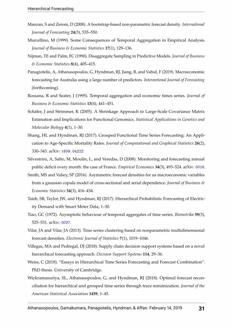
Table 3: Variables, Series IDs and their descriptions for Changes in Inventories - Expenditure Approach


GneCii A2302562X Changes in InventoriesGneCiiPfm A2302560V FarmGneCiiPba A2302561W Public authoritiesGneCiiPnf A2302559K Private; Non-farm TotalGneCiiPnfMin A83722619L Private; Mining (B)

GneCiiPnfMan A3348511X Private; Manufacturing (C)GneCiiPnfWht A3348512A Private; Wholesale trade (F)GneCiiPnfRet A3348513C Private; Retail trade (G)GneCiiPnfOnf A2302273C Private; Non-farm; Other non-farm industries

Table 4: Variables, Series IDs and their descriptions for Household Final Consumption - ExpenditureApproach


GneDfdHfc A2302254W Household Final Consumption ExpenditureGneDfdFceHfcFud A2302237V FoodGneDfdFceHfcAbt A3605816F Alcoholic beverages and tobaccoGneDfdFceHfcAbtCig A2302238W Cigarettes and tobaccoGneDfdFceHfcAbtAlc A2302239X Alcoholic beverages

GneDfdFceHfcCnf A2302240J Clothing and footwearGneDfdFceHfcHwe A3605680F Housing, water, electricity, gas and other fuelsGneDfdFceHfcHweRnt A3605681J Actual and imputed rent for housingGneDfdFceHfcHweWsc A3605682K Water and sewerage chargesGneDfdFceHfcHweEgf A2302242L Electricity, gas and other fuel

GneDfdFceHfcFhe A2302243R Furnishings and household equipmentGneDfdFceHfcFheFnt A3605683L Furniture, floor coverings and household goodsGneDfdFceHfcFheApp A3605684R Household appliancesGneDfdFceHfcFheTls A3605685T Household toolsGneDfdFceHfcHlt A2302244T Health

GneDfdFceHfcHltMed A3605686V Medicines, medical aids and therapeutic appliancesGneDfdFceHfcHltHsv A3605687W Total health servicesGneDfdFceHfcTpt A3605688X TransportGneDfdFceHfcTptPvh A2302245V Purchase of vehiclesGneDfdFceHfcTptOvh A2302246W Operation of vehicles

GneDfdFceHfcTptTsv A2302247X Transport servicesGneDfdFceHfcCom A2302248A CommunicationsGneDfdFceHfcRnc A2302249C Recreation and cultureGneDfdFceHfcEdc A2302250L Education servicesGneDfdFceHfcHcr A2302251R Hotels, cafes and restaurants

GneDfdFceHfcHcrCsv A3605694V Catering servicesGneDfdFceHfcHcrAsv A3605695W Accommodation servicesGneDfdFceHfcMis A3605696X Miscellaneous goods and servicesGneDfdFceHfcMisOgd A3605697A Other goodsGneDfdFceHfcMisIfs A2302252T Insurance and other financial servicesGneDfdFceHfcMisOsv A3606485T Other services


Hierarchical Forecasting · Hierarchical Forecasting approaches rather than single level approaches...

Documents

Transcript of Hierarchical Forecasting · Hierarchical Forecasting approaches rather than single level approaches...