Hidden Markov Models -- Introduction

Introduction

All prior models of speech are nonparametric and non--statistical.

Hence estimates of Variables are uniformed by the relative deviations of models

Hidden Markov Models – An attempt to reproduce the statistical fluctuation in

speech across a small utterance – An attempt which has a training theory which is

well motivated

This Lecture

What is a Hidden Markov Model What are the various types of estimation

procedures used How does one optimize the performance of a hidden Markov Model. How can the model be extended to more general cases of models.

Agenda

Markov Chains -- How to estimate probabilities Hidden Markov Models

– definition – how to identify – how to choose parameters – how to optimize parameters to produce the best

models Types of Hidden Markov Models

Agenda II

Next Lecture Different Type of Hidden Markov Models. – Distinct implimentation details.

Overview Techniques of Choosing Hidden Markov

Models and estimating parameters Related to Dynamic Programming already done. Quantities Recursively defined Key Difference

– Can estimate true probabilities and effectively variances and weight estimates

– Estimation Time Surprisingly fast.

Vocabulary Hidden Markov Model

– Much more below, but a doubly stochastic model, the underlying states are Markov, the output states are produced by a random process.

Alpha Terminal, Beta Terminal – Alpha terminal, the probability of the initial portion

of a state sequence given it ends in a particular state. – Beta terminal, the probability that a terminal

sequence starts in state s

Vocabulary II Maximum Likelihood Estimation

– Choosing parameters of the set so that the probability of the observation sequence is Maximized

– The classical principle for statistical inference, others benchmarked against MLE

Sufficient Statistics. – Functions of the input data which bear on the parametric

form of the distribution.

– If you know the sufficient statistics you know everything that the data can provide about the unknown parameters

Vocabulary III

Jensen’s Inequality

– For convex functions and any probability distribution

E(f(x))>f(E(x)) I.e. E(X*X)>=E(x)*E(x)

– For concave functions E(log(x))<=logE(x)

Hidden Markov Models Introduction to the basic properties of

discrete Markov Chains, their relationship to Hidden Markov Models

Definition of a Hidden Markov Model Their use in discrete word recognition Techniques to Evaluate and Train Discrete

Hidden Markov Models

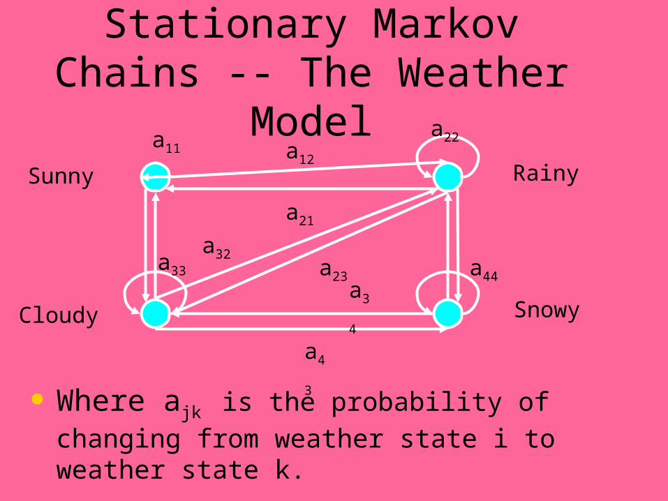
Stationary Markov Chains -- The Weather Model

Where ajk is the probability of changing from

weather state i to weather state k.

Sunny

Cloudy

Rainy

Snowy

a12

a22

a33 a44

a11

a21

a32a23

a34

a43

Facts About the Weather Model As drawn the model is recurrent, I.e. any state

can connect to any other, this structure is an assumption of the model Transition probabilities are “directly observable” in the sense that one can average numbers of transitions of an observed type from a given observed state For Example, one can calculate the average number of times that it rains in the next epoch given its cloudy now.

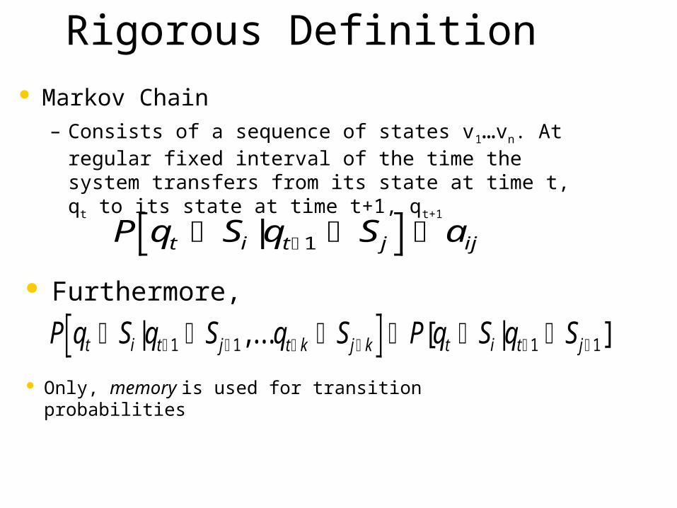
Rigorous Definition Markov Chain

– Consists of a sequence of states v1…vn. At regular fixed interval of the time the system transfers from its state at time t, qt to its state at time t+1, qt+1

P q S q S at i t j ij | 1

Furthermore,

P q S q S q S P q S q St i t j t k j k t i t j | ,... [ | ]1 1 1 1

Only, memory is used for transition probabilities

Hidden Markov ModelHidden Markov ModelVs Markov ChainVs Markov Chain

Markov chains have entirely observable states. However a “Hidden Markov Model” is a model of a Markov Source which admits an element each time slot depending upon the state. The states are not directly observed

For instance...

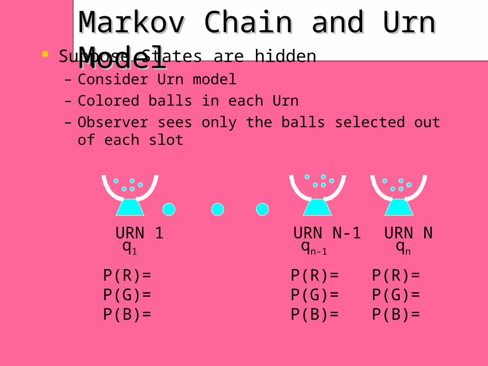
Markov Chain and Urn ModelMarkov Chain and Urn Model Suppose States are hidden

– Consider Urn model

– Colored balls in each Urn

– Observer sees only the balls selected out of each slot

q1 qn-1 qn

URN N-1 URN 1 URN N

P(R)= P(G)= P(B)=

P(R)= P(G)= P(B)=

P(R)= P(G)= P(B)=

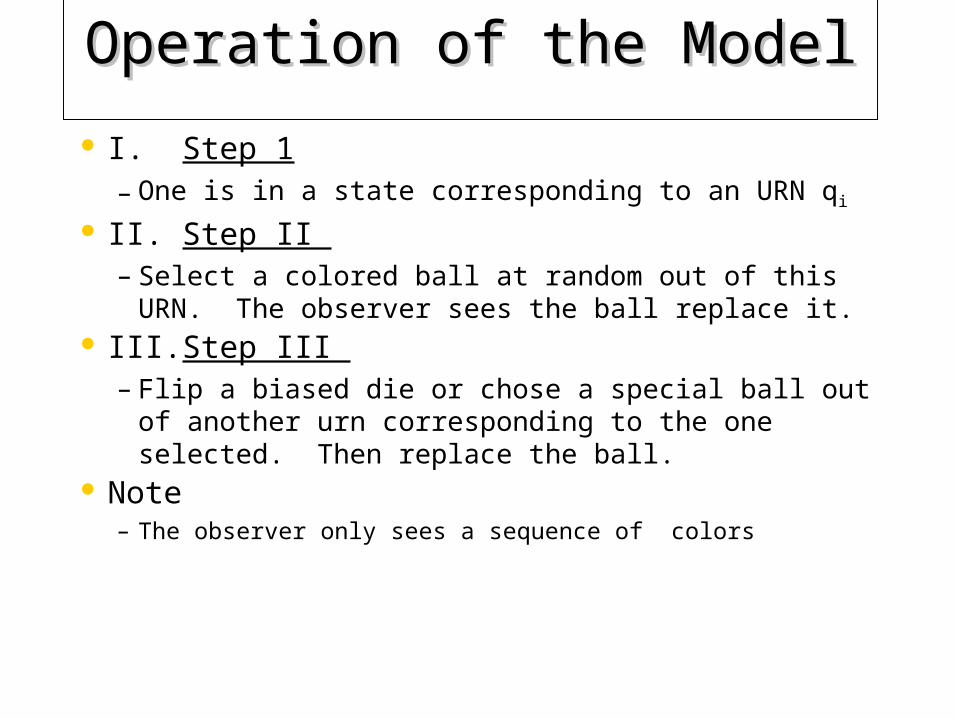
Operation of the ModelOperation of the Model

I. Step 1 – One is in a state corresponding to an URN qi

II. Step II – Select a colored ball at random out of this URN. The

observer sees the ball replace it. III.Step III

– Flip a biased die or chose a special ball out of another urn corresponding to the one selected. Then replace the ball.

Note – The observer only sees a sequence of colors

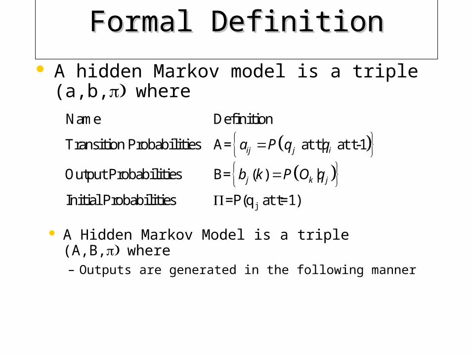
Formal DefinitionFormal Definition

A hidden Markov model is a triple (a,b,where

j

Name Definition

Transition Probabilities A= at t| at t-1

Output Probabilities B= ( ) |

Initial Probabilities =P(q at t=1)

ij j i

j k j

a P q q

b k P O q

A Hidden Markov Model is a triple (A,B,where – Outputs are generated in the following manner

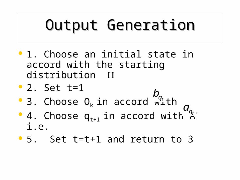
Output GenerationOutput Generation

1. Choose an initial state in accord with the starting distribution

2. Set t=1 3. Choose Ok in accord with 4. Choose qt+1 in accord with A i.e. 5. Set t=t+1 and return to 3

bqt

aqt .

Problems Using Hidden Problems Using Hidden Markov ModelsMarkov Models

Its hard a priori to say what is the best structure for a HMM for a given problem. – Empirically, many models of a given complexity often

produce a similar fit, hence its hard to identify models. It’s possible now, due to Amari, to say whether or

not two models are stochastically equivalent. I.E. Generate same proabilities, – Metric on HMM’s. – (Usually probability 0).

Criticism Leveled Against Criticism Leveled Against HMM’s: Somewhat BogusHMM’s: Somewhat Bogus

For a hidden Markov model – The past history is reflected only in the last state that

the sequence is in. Therefore prior history cannot be influencing result. Speech because of coarticulation is dependent upon prior history. /pinz/ /pits/

There can be no backward effects. – There can be no effects of “future” utterances on

present, I.e. backwards assimilation, – grey chips, Vs grey ship., great chip

Answers to CriticismAnswers to Criticism

First Objection. – Markov model by itself cannot handle this

elementary. However, distortion coefficients delta coefficients effectively convey framed information about locally prior parts of the utterance.

Second Objection – Shows that speech has to be locally buffered and

conclusion about a phoneme cannot be made without a limited lookahead like people due. Can easily construct a Markov model to do this

No ideal method to determineNo ideal method to determine Best Model for Phone, Word Sentence. However,

– In fact, they are the only existing statistical models of speech recognition.

– Can be use to self--validate as well as recognize, validate significance

SummarySummary

Cannot Directly identify HMM structure, however, can still use model and assume the speech source obeys the given structure.

BUT – If cannot choose suitable parameters for the

model it turns out to be useless. – This problem has been solved

HistoryHistory Technique originated by Leonard Baum.

– Baum (1966), Author, wrote 3 or 4 papers, math journals.

– Probably most important innovation in mathematical statistics, at time.

Took about 10 years for Fred Jelinek and baker to pick up for speech.

Now used all over the place, popularized by A.P. Dempster and Rubin at Harvard.

PreconditionsPreconditions

For speech recognition application suppose that frames are Vector Quantized codewords representing the speech signal See later Hidden Markov models can do their own quantization. However, this case treated first for simplicity.

Three Basic Prerequisites for Three Basic Prerequisites for Hidden Markov Model UseHidden Markov Model Use

Problem I – Given an observation sequence, O1,…OT and

how does one compute the probability P(O|

Problem II – Given the observation sequence O1,…OT how

can one find a state sequence which is optimal in some sense

Problem IIIProblem III Given a training sequence how do we train

the model O=O1…OT to maximize P(O|– Hidden Markov models are a form of maximal

likelihood estimation. In principal one can use them to do statistical tests of hypotheses, in particular tests values of certain parameters …

– Maximal Likelihood estimation is a method which is know to be asymptotically optimal for estimating the parameters. Implicitly minimizing the probability of error sequences.

–

Solutions to the Three Hidden Solutions to the Three Hidden Markov ProblemsMarkov Problems

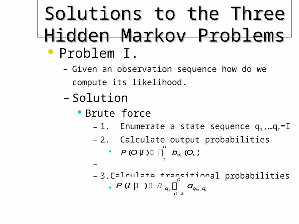
Problem I. – Given an observation sequence how do we compute its likelihood. – Solution

Brute force – 1. Enumerate a state sequence q1,…qt=I

– 2. Calculate output probabilities

•

–

– 3.Calculate transitional probabilities

• .

P O I b Oq i

n

i( | ) ( )

1

P I aq q qi

n

i i( | )

1 12

Problem I, Brute Force Problem I, Brute Force ContinuedContinued

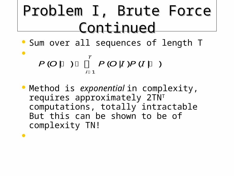
Sum over all sequences of length T

Method is exponential in complexity, requires approximately 2TNT computations, totally intractable But this can be shown to be of complexity TN!

P O P O I P Ii

T

( | ) ( | ) ( | )

1

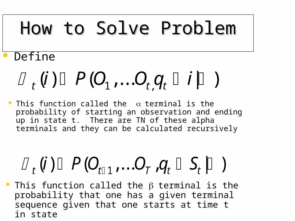
How to Solve ProblemHow to Solve Problem Define

t t ti P O O q i( ) ( ,... | ), 1 This function called the terminal is the probability of

starting an observation and ending up in state t. There are TN of these alpha terminals and they can be calculated recursively

t t T t ti P O O q S( ) ( ,... , | ) 1 This function called the terminal is the

probability that one has a given terminal sequence given that one starts at time t in state

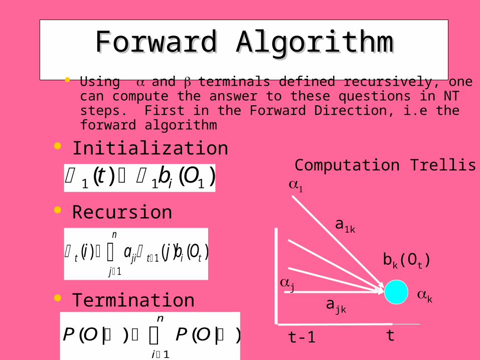
Forward AlgorithmForward Algorithm Using and terminals defined recursively, one can

compute the answer to these questions in NT steps. First in the Forward Direction, i.e the forward algorithm

Initialization

Recursion

1 1 1( ) ( )t b Oi

t ji tj

n

i ti a j b O( ) ( ) ( ) 1

1

Termination

P O P Oi

n

( | ) ( | )

1

t-1 t

j k

a1k

ajk

Computation Trellis

bk(Ot)

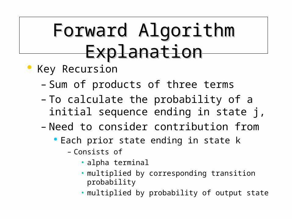
Forward Algorithm Forward Algorithm ExplanationExplanation

Key Recursion – Sum of products of three terms – To calculate the probability of a initial

sequence ending in state j, – Need to consider contribution from

Each prior state ending in state k – Consists of

• alpha terminal

• multiplied by corresponding transition probability

• multiplied by probability of output state

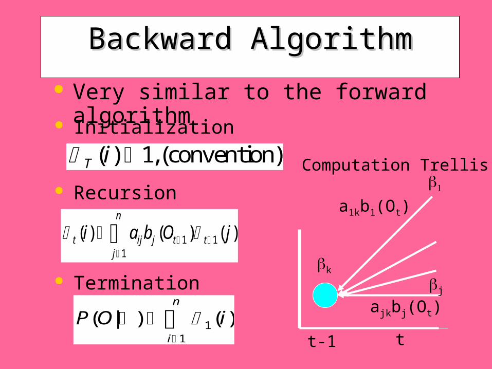
Backward AlgorithmBackward Algorithm

Very similar to the forward algorithm Initialization

Recursion

T i( ) ,( 1 convention)

t ij j t tj

n

i a b O j( ) ( ) ( ) 1 1

1

Termination

P O ii

n

( | ) ( ) 1

1 t-1 t

j

k

a1kb1(Ot)

ajkbj(Ot)

Computation Trellis

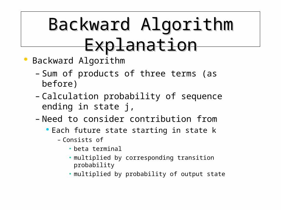
Backward Algorithm Backward Algorithm ExplanationExplanation

Backward Algorithm – Sum of products of three terms (as before) – Calculation probability of sequence ending in

state j, – Need to consider contribution from

Each future state starting in state k – Consists of

• beta terminal

• multiplied by corresponding transition probability

• multiplied by probability of output state

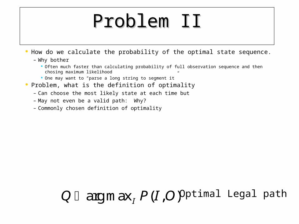
Problem IIProblem II

How do we calculate the probability of the optimal state sequence. – Why bother

Often much faster than calculating probability of full observation sequence and then chosing maximum likelihood

One may want to “parse a long string to segment it”

Problem, what is the definition of optimality – Can choose the most likely state at each time but – May not even be a valid path: Why? – Commonly chosen definition of optimality

Q P I OI arg max ( , ) Optimal Legal path

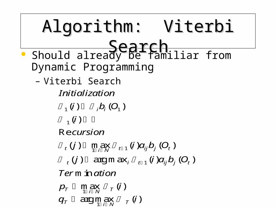
Algorithm: Viterbi SearchAlgorithm: Viterbi Search

Should already be familiar from Dynamic Programming – Viterbi Search

Initialization

i b O

i

cursion

j i a b O

j i a b O

Ter ation

p i

q i

i i

t i N t ij j t

t i t ij j t

T i N T

T i N T

1 1

1

1 1

1

1

1

( ) ( )

( )

Re

( ) max ( ) ( )

( ) arg max ( ) ( )

min

max ( )

arg max ( )

Viterbi SearchViterbi Search Principle Same as dynamic programming principle

discussed two lectures ago.

Frequent UseFrequent Use

Multitude of paths through full model.

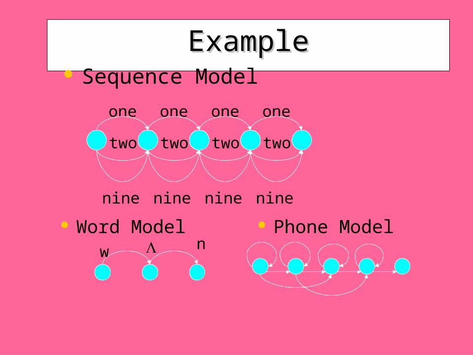
ExampleExample Sequence Model

one

two

nine

one

two

nine

one

two

nine

one

two

nine

Word Modelw n

Phone Model

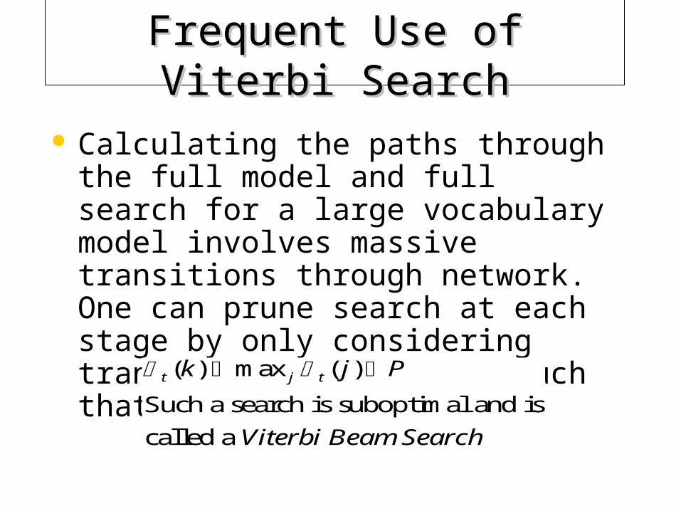
Frequent Use of Viterbi Frequent Use of Viterbi SearchSearch

Calculating the paths through the full model and full search for a large vocabulary model involves massive transitions through network. One can prune search at each stage by only considering transitions from states such that

t j tk j P( ) max ( )

Such a search is suboptimal and is

called a Viterbi Beam Search

Problem IIIProblem III

How do we train model given multiple observation sequences – No known way analytically to find formula

which maximizes the probability of an observation sequence. There is an iterative procedure (Baum--Welsh) update, or EM algorithm which always increases P(O|until maximim is achieved

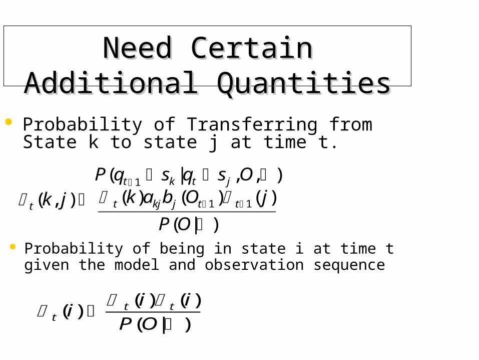
Need Certain Additional Need Certain Additional QuantitiesQuantities

Probability of Transferring from State k to state j at time t.

t

t k t j

t kj j t tk j

P q s q s Ok a b O j

P O

( , )

( | , , )( ) ( ) ( )

( | )

1

1 1

t

t tii i

P O( )

( ) ( )

( | )

Probability of being in state i at time t given the model and observation sequence

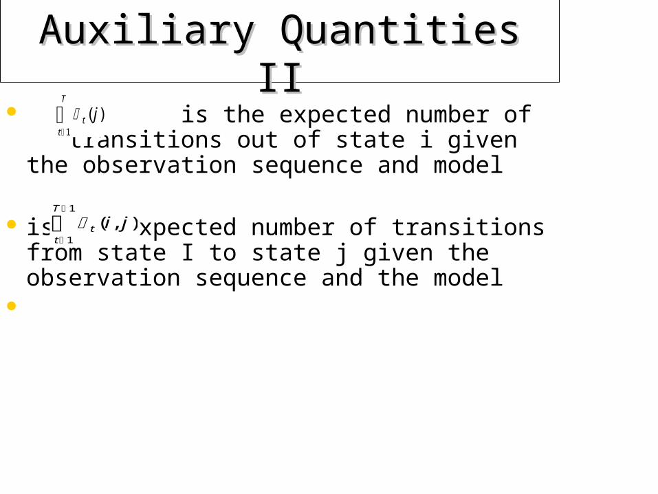
Auxiliary Quantities IIAuxiliary Quantities II

is the expected number of transitions out of state i given the observation sequence and model

is the expected number of transitions from state I to state j given the observation sequence and the model

tt

T

j( )

1

tt

T

i j( , )

1

1

Baum Welch reupdate: EM Baum Welch reupdate: EM algorithmalgorithm

Start with estimates for (A,B,)

Reestimate the parameters by calculating their most likely value. This amounts to in this case replacing the parameters by their expected value.

Given the observations estimate the sufficient statistics of the model, which are

t t t, ,

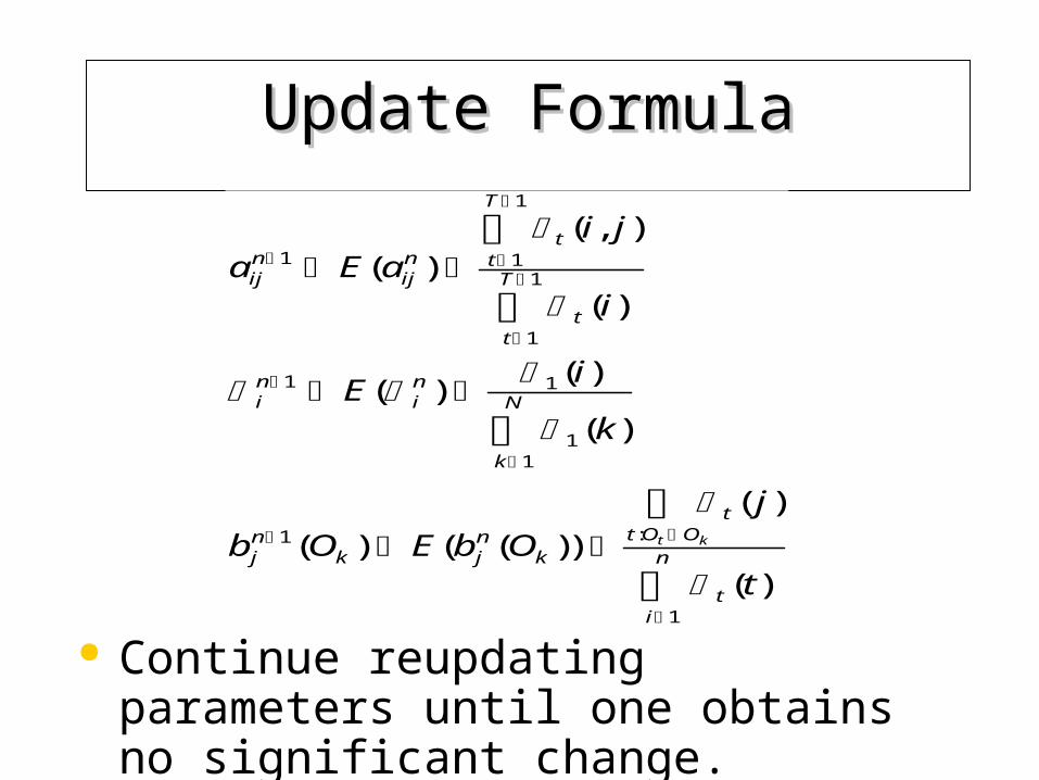
Update FormulaUpdate Formula

Continue reupdating parameters until one obtains no significant change.

a E ai j

i

Ei

k

b O E b O

j

t

ijn

ijn

tt

T

tt

T

in

in

k

N

jn

k jn

k

tt O O

ti

nt k

1 1

1

1

1

1 1

11

1

1

( )( , )

( )

( )( )

( )

( ) ( ( ))

( )

( )

:

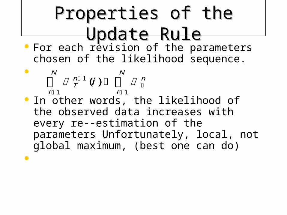
Properties of the Update RuleProperties of the Update Rule

For each revision of the parameters chosen of the likelihood sequence.

In other words, the likelihood of the observed data increases with every re--estimation of the parameters Unfortunately, local, not global maximum, (best one can do)

Tn n

i

N

i

N

i

1

11

( )

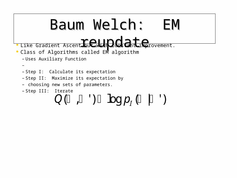
Baum Welch: EM reupdateBaum Welch: EM reupdate Like Gradient Ascent but with constant improvement. Class of Algorithms called EM algorithm

– Uses Auxiliary Function – – Step I: Calculate its expectation – Step II: Maximize its expectation by – choosing new sets of parameters. – Step III: Iterate

Q pI( , ' ) log ( | ' )

EM interpretationEM interpretation

Auxiliary Function is Log probability of an observation sequence for a set of transitions Its natural to believe that if we maximize the expectation of the log probability then the by changing parameters the the overall log probability, likelihood will increase.

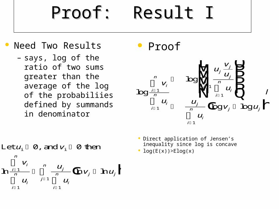
Proof: Result IProof: Result I

Need Two Results – says, log of the ratio of

two sums greater than the average of the log of the probabiliies defined by summands in denominator

Let and then

ln

i iu v

v

u

u

uv u

ii

n

ii

nj

ii

nj

n

j j

0 0

1

1 1

1

,

ln lnc h

Proof

logv

u

uv

u

u

u

uv u

li

i

n

ii

n

jj

j

ii

nj

n

j

ii

n j j

L

N

MMMM

O

Q

PPPP

1

1

1

1

1

log

log logc h

Direct application of Jensen’s inequality since log is concave

log(E(x))>Elog(x)

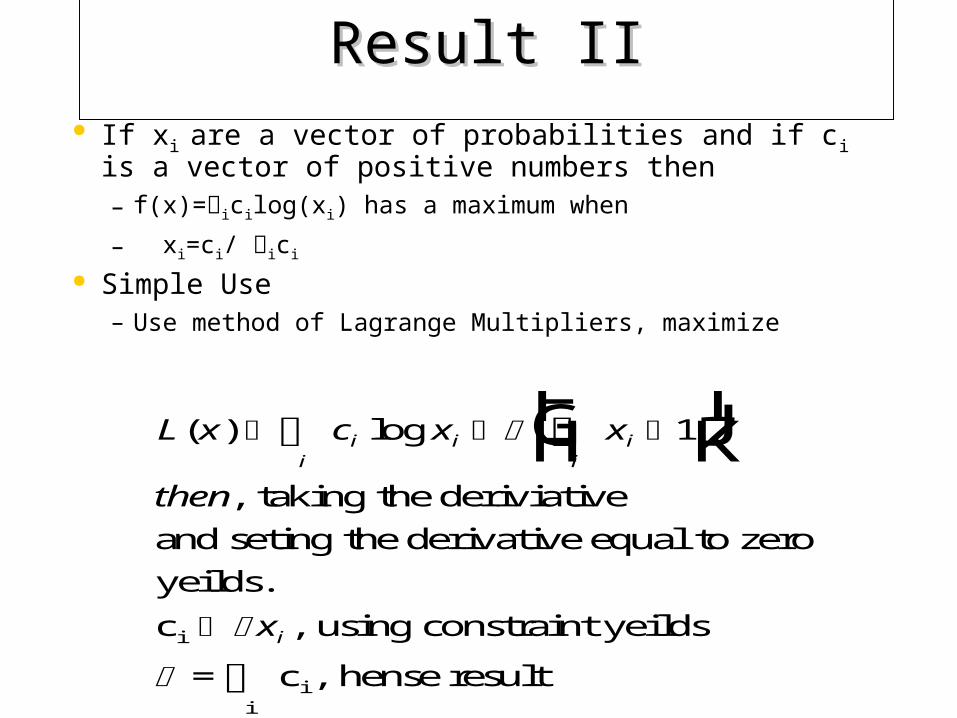
Result IIResult II If xi are a vector of probabilities and if ci is a vector of positive

numbers then – f(x)=icilog(xi) has a maximum when

– xi=ci/ ici

Simple Use – Use method of Lagrange Multipliers, maximize

L x c x x

then

x

i i iii

i

( ) log

,

,

,

FHG

IKJ

1

taking the deriviative

and seting the derivative equal to zero

yeilds.

c using constraint yeilds

= c hense result

i

ii

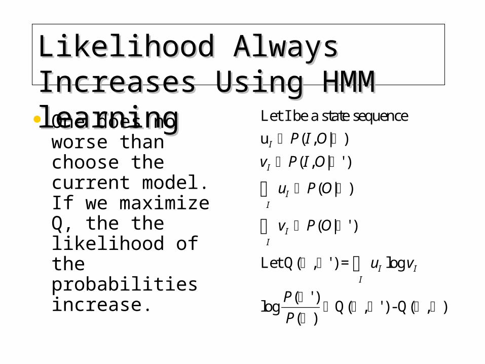
Likelihood Always Increases Likelihood Always Increases Using HMM learningUsing HMM learning

One does no worse than choose the current model. If we maximize Q, the the likelihood of the probabilities increase.

Let I be a state sequence

u

Let Q( , ' ) =

Q( , ' ) - Q( , )

I

I

II

II

I II

P I O

v P I O

u P O

v P O

u v

P

P

( , | )

( , | ' )

( | )

( | ' )

log

log( ' )

( )

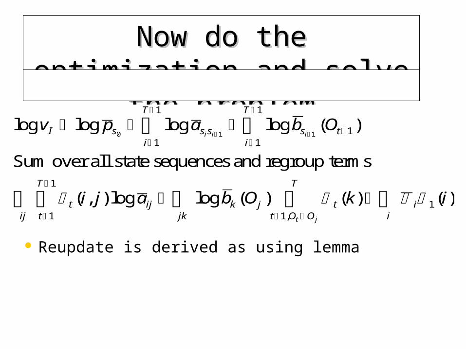
Now do the optimization and Now do the optimization and solve the problemsolve the problem

log log log log ( )

( , ) log log ( ) ( ) ( ),

v p a b O

i j a b O k i

I s s s s ti

T

i

T

t ijt

T

ijk

jkj t i

it O O

T

i i i

t j

0 1 1 11

1

1

1

1

1

11

Sum over all state sequences and regroup terms

Reupdate is derived as using lemma

Properties of Reupdate RuleProperties of Reupdate RuleStructure of the model is preserved. For parameters which sum to one. n+1=f(P), Therefore if a parameter starts out zero in will stay as zero. If parameters start out as 1 and represent probabilities they stay as sure event.

Generalizations of Hidden Generalizations of Hidden Markov Models: Very Flexible Markov Models: Very Flexible

Explicitly modeling state duration: Next lecture Continuous state density hidden Markov models. Very general models can be done next lecture Other variants of EM algorithm: --backprop, next lecture Continuous time densiites: next time I teach!

Tied StatesTied States

Its quite possible to force states to have the same transition probabilities. All events which mention the same state are pooled. If events updating probabilities on two nodes are pooled and they start out equal, they will end up equal

Null Transitions: Original IBM Null Transitions: Original IBM ModelModel

IBM Hidden Markov – For clarity in presentation models presented

where observations are associated with states. – However, models might very well be

constructed where outputs are associated with transitions.

– In this case, its useful to have models where null transitions exist. I.e. Jumps from a state to another produces no output.

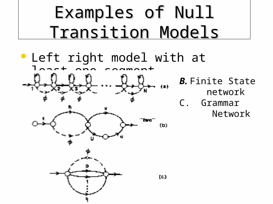
Examples of Null Transition Examples of Null Transition ModelsModels

Left right model with at least one segment

B. Finite State network C. Grammar Network

Speech ModelSpeech Model

Speech Model is Usually not fully recurrent. – Use one or another variant of left to right model

Lack of full recurrence for model. No problem structure is preserved.

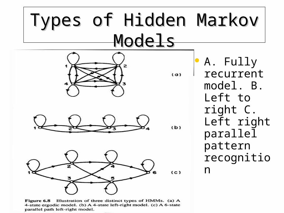
Types of Hidden Markov Types of Hidden Markov ModelsModels

A. Fully recurrent model. B. Left to right C. Left right parallel pattern recognition

Summary: Intro to HMM’sSummary: Intro to HMM’s

Presented Markov chains Defined Hidden Markov Models

– showed that difficult to estimate parameters Discussed basic method of estimating

parameters and segmenting speech

Summary II:Summary II:

Showed how Baum Welch reupdate leads to ever increasing likelihood – Better than classical gradient ascent.

Different types of Markov Models – tied states – null transitions

Not Covered IINot Covered II

Continuous time Hidden Markov Models Continuous State Hidden Markov Models Additional Material

Additional MaterialAdditional Material

Not much theoretical despite much use use. Eliot et. al. Lipster and Shiraev …. Blizzard of Applied material.