Hidden Markov Models & EMData-Intensive Information Processing Applications ― Session #8

Nitin MadnaniUniversity of Maryland

Tuesday, March 30, 2010

This work is licensed under a Creative Commons Attribution-Noncommercial-Share Alike 3.0 United StatesSee http://creativecommons.org/licenses/by-nc-sa/3.0/us/ for details

Source: Wikipedia (Japanese rock garden)

Today’s Agenda Need to cover lots of background material

Introduction to Statistical Models Hidden Markov Models Part of Speech Tagging Applying HMMs to POS tagging Expectation-Maximization (EM) Algorithm

Now on to the Map Reduce stuff Training HMMs using MapReduce

• Supervised training of HMMs• Rough conceptual sketch of unsupervised training using EM

Introduction to statistical models Until the 1990s, text processing relied on rule-based

systems

Advantages More predictable Easy to understand Easy to identify errors and fix them

Disadvantages Extremely labor-intensive to create Not robust to out of domain input No partial output or analysis when failure occurs

Introduction to statistical models A better strategy is to use data-driven methods

Basic idea: learn from a large corpus of examples of what we wish to model (Training Data)

Advantages More robust to the complexities of real-world input Creating training data is usually cheaper than creating rules

• Even easier today thanks to Amazon Mechanical Turk• Data may already exist for independent reasons

Disadvantages Systems often behave differently compared to expectations Hard to understand the reasons for errors or debug errors

Introduction to statistical models Learning from training data usually means estimating the

parameters of the statistical model

Estimation usually carried out via machine learning

Two kinds of machine learning algorithms

Supervised learning Training data consists of the inputs and respective outputs (labels) Labels are usually created via expert annotation (expensive) Difficult to annotate when predicting more complex outputs

Unsupervised learning Training data just consists of inputs. No labels. One example of such an algorithm: Expectation Maximization

Hidden Markov Models (HMMs)

A very useful and popular statistical model

Finite State Machines What do we need to specify an FSM formally ?

Finite number of states Transitions Input alphabet Start state Final state(s)

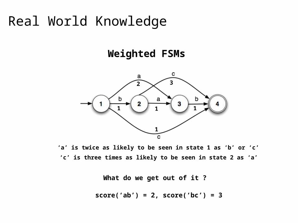
Real World Knowledge

‘a’ is twice as likely to be seen in state 1 as ‘b’ or ‘c’

‘c’ is three times as likely to be seen in state 2 as ‘a’

Weighted FSMs

2

1

1

1

3

1

What do we get out of it ?

score(‘ab’) = 2, score(‘bc’) = 3

Real World Knowledge

‘a’ is twice as likely to be seen in state 1 as ‘b’ or ‘c’

‘c’ is three times as likely to be seen in state 2 as ‘a’

Probabilistic FSMs

What do we get out of it ?

P(‘ab’) = 0.50 * 1.00 = 0.5, P(‘bc’) = 0.25 * 0.75 = 0.1875

0.5

0.25

0.25

0.25

0.75

1.0

Markov Chains

This not a valid prob. FSM! No start states

Use prior probabilities

Note that prob. of being in any state ONLY depends on previous state ,i.e., the (1st order) Markov assumption

This extension of a prob.FSM is called a Markov Chain or an Observed Markov Model

Each state corresponds to an observable physical event

0.5

0.2 0.3

Are states always observable?

1, 2, 3, 4, 5, 6Day:

Bu, Be, S, Be, S, Bu

Bu: Bull Market Be: Bear Market S : Static Market

Here’s what you actually observe:

1, 2, 3, 4, 5, 6Day: ↑: Market is up ↓: Market is down ↔: Market hasn’t changed↑ ↓ ↔ ↑ ↓ ↔

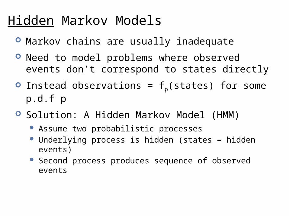
Hidden Markov Models Markov chains are usually inadequate

Need to model problems where observed events don’t correspond to states directly

Instead observations = fp(states) for some p.d.f p

Solution: A Hidden Markov Model (HMM) Assume two probabilistic processes Underlying process is hidden (states = hidden events) Second process produces sequence of observed events

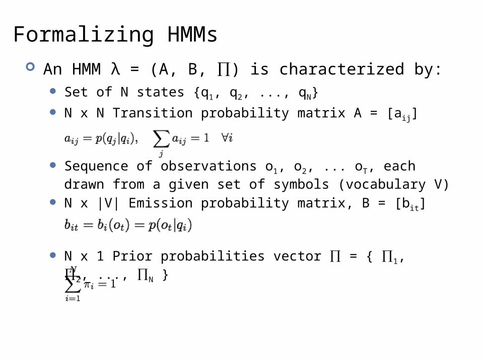
Formalizing HMMs An HMM λ = (A, B, ∏) is characterized by:

Set of N states {q1, q2, ..., qN}

N x N Transition probability matrix A = [aij]

Sequence of observations o1, o2, ... oT, each drawn from a given set of symbols (vocabulary V)

N x |V| Emission probability matrix, B = [bit]

N x 1 Prior probabilities vector ∏ = { ∏1, ∏2, ..., ∏N }

Things to know about HMMs The (first-order) Markov assumption holds

The probability of an output symbol depends only on the state generating it

The number of states (N) does not have to equal the number of observations (T)

Stock Market HMM

States ✓Transitions ✓

Valid ✓

Vocabulary ✓

Emissions ✓Valid ✓

∏1=0.5 ∏2=0.2 ∏3=0.3

Priors ✓Valid ✓

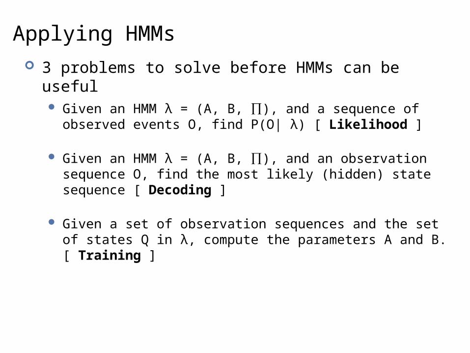
Applying HMMs 3 problems to solve before HMMs can be useful

Given an HMM λ = (A, B, ∏), and a sequence of observed events O, find P(O| λ) [ Likelihood ]

Given an HMM λ = (A, B, ∏), and an observation sequence O, find the most likely (hidden) state sequence [ Decoding ]

Given a set of observation sequences and the set of states Q in λ, compute the parameters A and B. [ Training ]

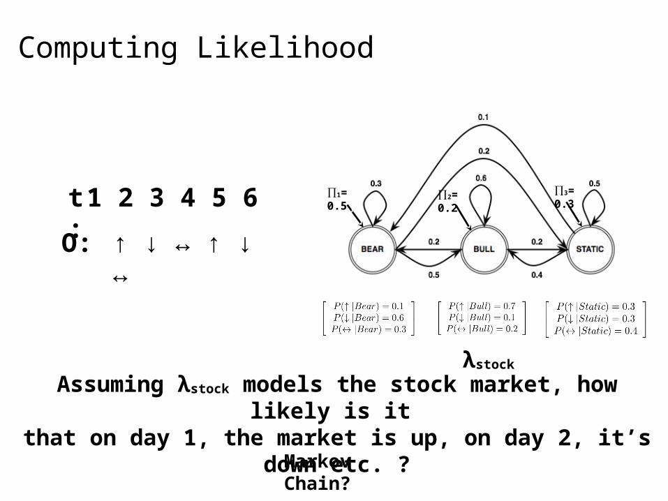
Computing Likelihood

1 2 3 4 5 6

↑ ↓ ↔ ↑ ↓ ↔

t:

O:

Assuming λstock models the stock market, how likely is it that on day 1, the market is up, on day 2, it’s down etc. ?

∏1=0.5

∏2=0.2

∏3=0.3

Markov Chain?

λstock

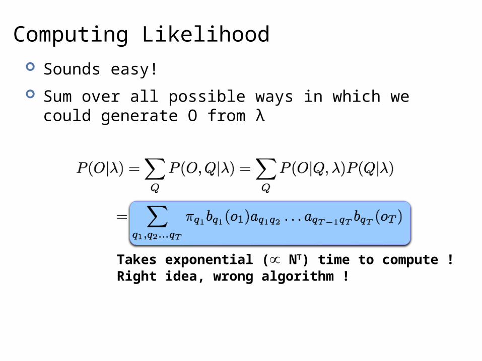
Computing Likelihood Sounds easy!

Sum over all possible ways in which we could generate O from λ

Takes exponential (∝ NT) time to compute !Right idea, wrong algorithm !

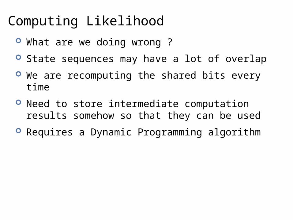
Computing Likelihood What are we doing wrong ?

State sequences may have a lot of overlap

We are recomputing the shared bits every time

Need to store intermediate computation results somehow so that they can be used

Requires a Dynamic Programming algorithm

20

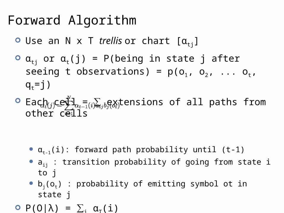
Forward Algorithm Use an N x T trellis or chart [αtj]

αtj or αt(j) = P(being in state j after seeing t observations) = p(o1, o2, ... ot, qt=j)

Each cell = ∑ extensions of all paths from other cells

αt-1(i): forward path probability until (t-1)

aij : transition probability of going from state i to j

bj(ot) : probability of emitting symbol ot in state j

P(O|λ) = ∑i αT(i)

Polynomial time ( N∝ 2T)

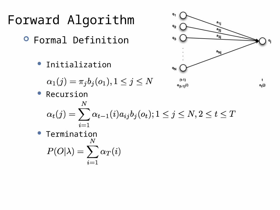
Forward Algorithm Formal Definition

Initialization

Recursion

Termination

22

23

Forward Algorithm

Bear

Bull

Static

stat

es

time

↑ ↓ ↑t=1 t=2 t=3

↑ ↓ ↑O =

find P(O|λstock)

24

Forward Algorithm (Initialization)

Bear

Bull

Static

stat

es

time

↑ ↓ ↑t=1 t=2 t=3

α1(Bu)0.2*0.7=0.14

0.5*0.1=0.05

0.3*0.3=0.09

25

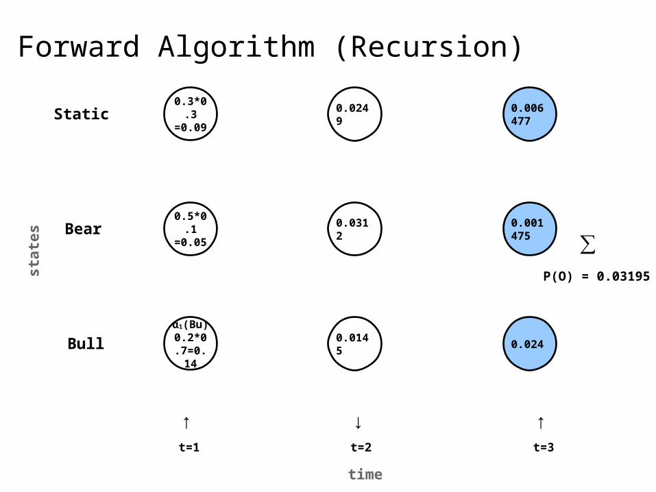
Forward Algorithm (Recursion)

Bear

Bull

Static

stat

es

time

↑ ↓ ↑t=1 t=2 t=3

α1(Bu)0.2*0.7=0.14

0.5*0.1=0.05

0.3*0.3=0.09

0.0145

α1(Bu) * aBuBu * bBu(↓)0.14 * 0.6 * 0.1=0.0084

0.05 * 0.5 * 0.1 =0.0025

0.09 * 0.4 * 0.1 =0.0036

∑

.... and so on

26

Forward Algorithm (Recursion)

Bear

Bull

Static

stat

es

time

↑ ↓ ↑t=1 t=2 t=3

α1(Bu)0.2*0.7=0.14

0.5*0.1=0.05

0.3*0.3=0.09

0.0145

0.0312

0.0249

0.024

0.001475

0.006477

27

Forward Algorithm (Recursion)

Bear

Bull

Static

stat

es

time

↑ ↓ ↑t=1 t=2 t=3

α1(Bu)0.2*0.7=0.14

0.5*0.1=0.05

0.3*0.3=0.09

0.0145

0.0312

0.0249

0.024

0.001475

0.006477

∑P(O) = 0.03195

Decoding

1 2 3 4 5 6

↑ ↓ ↔ ↑ ↓ ↔

t:

O:

Given λstock as our model and O as our observations, what are the most likely states the market went through to produce O ?

∏1=0.5

∏2=0.2

∏3=0.3

λstock

Decoding “Decoding” because states are hidden

There’s a simple way to do it For each possible hidden state sequence, compute P(O) using

“forward algorithm” Pick the one that gives the highest P(O)

Will this give the right answer ?

Is it practical ?

29

Viterbi Algorithm Another dynamic programming algorithm

Same idea as the forward algorithm Store intermediate computation results in a trellis Build new cells from existing cells

Efficient (polynomial vs. exponential)

30

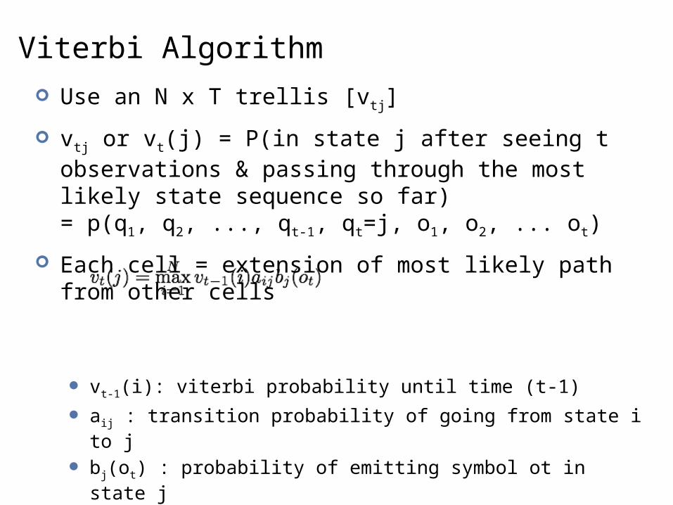
Viterbi Algorithm Use an N x T trellis [vtj]

vtj or vt(j) = P(in state j after seeing t observations & passing through the most likely state sequence so far) = p(q1, q2, ..., qt-1, qt=j, o1, o2, ... ot)

Each cell = extension of most likely path from other cells

vt-1(i): viterbi probability until time (t-1)

aij : transition probability of going from state i to j

bj(ot) : probability of emitting symbol ot in state j

P = maxi vT(i)

31

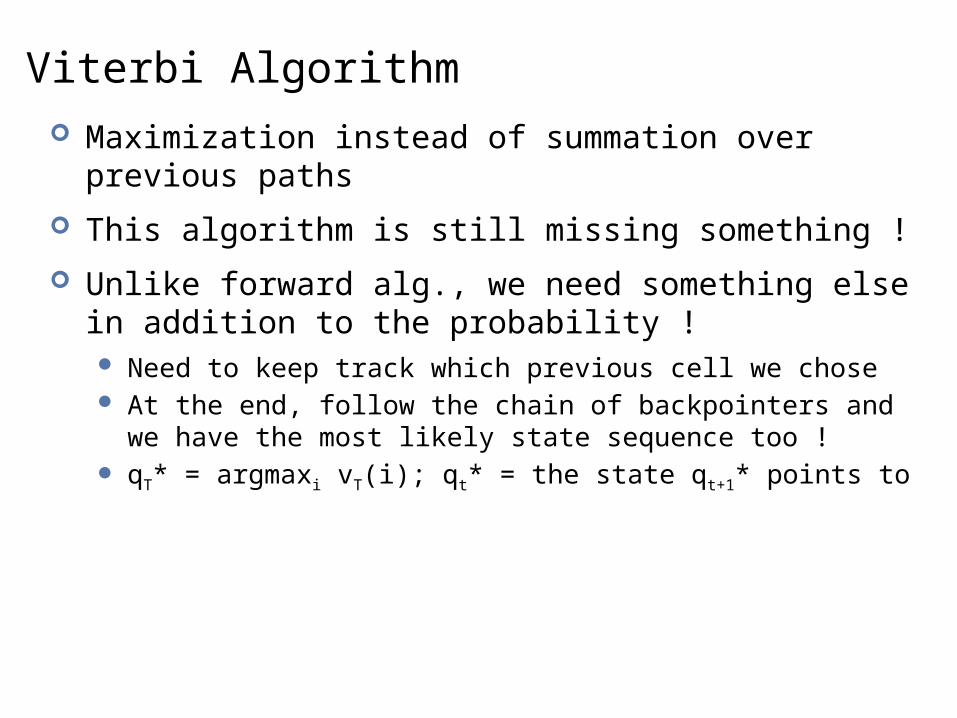
Viterbi Algorithm Maximization instead of summation over previous paths

This algorithm is still missing something !

Unlike forward alg., we need something else in addition to the probability ! Need to keep track which previous cell we chose At the end, follow the chain of backpointers and we have the most

likely state sequence too ! qT* = argmaxi vT(i); qt* = the state qt+1* points to

32

Viterbi Algorithm

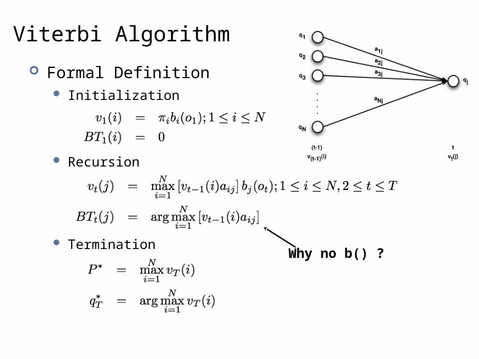
Formal Definition Initialization

Recursion

TerminationWhy no b() ?

34

Viterbi Algorithm

Bear

Bull

Static

stat

es

time

↑ ↓ ↑t=1 t=2 t=3

↑ ↓ ↑O =

find most likely given state sequence

35

Viterbi Algorithm (Initialization)

Bear

Bull

Static

stat

es

time

↑ ↓ ↑t=1 t=2 t=3

v1(Bu)0.2*0.7=0.14

0.5*0.1=0.05

0.3*0.3=0.09

36

Viterbi Algorithm (Recursion)

Bear

Bull

Static

stat

es

time

↑ ↓ ↑t=1 t=2 t=3

v1(Bu)0.2*0.7=0.14

0.5*0.1=0.05

0.3*0.3=0.09

0.0084

v1(Bu) * aBuBu * bBu(↓)0.14 * 0.6 * 0.1=0.0084

0.05 * 0.5 * 0.1 =0.0025

0.09 * 0.4 * 0.1 =0.0036

max

37

Viterbi Algorithm (Recursion)

Bear

Bull

Static

stat

es

time

↑ ↓ ↑t=1 t=2 t=3

v1(Bu)0.2*0.7=0.14

0.5*0.1=0.05

0.3*0.3=0.09

0.0084

.... and so on

38

Viterbi Algorithm (Recursion)

Bear

Bull

Static

stat

es

time

↑ ↓ ↑t=1 t=2 t=3

α1(Bu)0.2*0.7=0.14

0.5*0.1=0.05

0.3*0.3=0.09

0.0084

0.0168

0.0135

0.00588

0.000504

0.00202

39

Viterbi Algorithm (Termination)

Bear

Bull

Static

stat

es

time

↑ ↓ ↑t=1 t=2 t=3

v1(Bu)0.2*0.7=0.14

0.5*0.1=0.05

0.3*0.3=0.09

0.0084

0.0168

0.0135

0.00588

0.000504

0.00202

40

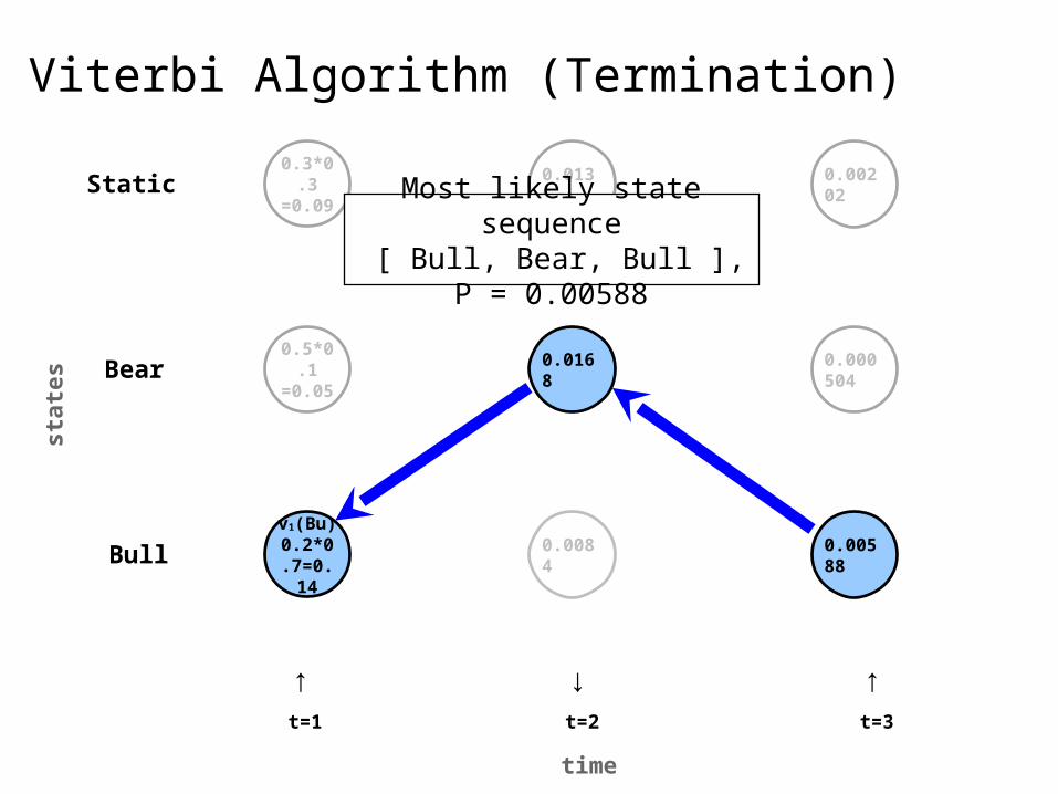
Viterbi Algorithm (Termination)

Bear

Bull

Static

stat

es

time

↑ ↓ ↑t=1 t=2 t=3

v1(Bu)0.2*0.7=0.14

0.5*0.1=0.05

0.3*0.3=0.09

0.0084

0.0168

0.0135

0.00588

0.000504

0.00202

Most likely state sequence [ Bull, Bear, Bull ], P = 0.00588

Why are HMMs useful? Models of data that is ordered sequentially

Recall sequence of market up/down/static observations

Other more useful sequences Words in a sentence Base pairs in a gene Letters in a word

Have been used for almost everything Automatic speech recognition Stock market forecasting (you thought I was joking?!) Aligning words in a bilingual parallel text Tagging words with parts of speech

Md. Rafiul Hassan and Baikunth Nath. Stock Market Forecasting Using Hidden Markov Models: A New Approach.Proceedings of the International Conference on Intelligent Systems Design and Applications.

Part of Speech Tagging

Part of Speech (POS) Tagging Parts of speech are well recognized linguistic entities

The Art of Grammar circa 100 B.C. Written to allow post-Classical Greek speakers to understand

Odyssey and other classical poets 8 classes of words

[Noun, Verb, Pronoun, Article, Adverb, Conjunction, Participle, Preposition]

Remarkably enduring list

Occur in almost every language

Defined primarily in terms of syntactic and morphological criteria (affixes)

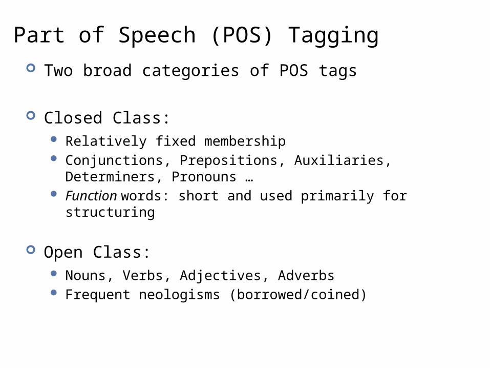
Part of Speech (POS) Tagging Two broad categories of POS tags

Closed Class: Relatively fixed membership Conjunctions, Prepositions, Auxiliaries, Determiners, Pronouns … Function words: short and used primarily for structuring

Open Class: Nouns, Verbs, Adjectives, Adverbs Frequent neologisms (borrowed/coined)

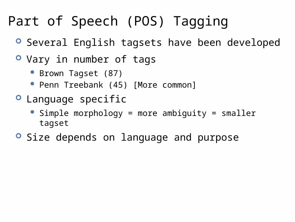
Part of Speech (POS) Tagging Several English tagsets have been developed

Vary in number of tags Brown Tagset (87) Penn Treebank (45) [More common]

Language specific Simple morphology = more ambiguity = smaller tagset

Size depends on language and purpose

Part of Speech (POS) Tagging

POS Tagging: The process of assigning “one” POS or other lexical class marker to each word in a corpus

Why do POS tagging? Corpus-based Linguistic Analysis & Lexicography

Information Retrieval & Question Answering

Automatic Speech Synthesis

Word Sense Disambiguation

Shallow Syntactic Parsing

Machine Translation

Why is POS tagging hard? Not really a lexical problem

Sequence labeling problem

Treating it as lexical problem runs us smack into the wall of ambiguity

I thought that you ... (that: conjunction)That day was nice (that: determiner)You can go that far (that: adverb)

HMMs & POS Tagging

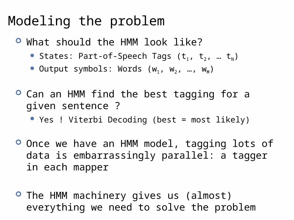
Modeling the problem What should the HMM look like?

States: Part-of-Speech Tags (t1, t2, … tN)

Output symbols: Words (w1, w2, …, wM)

Can an HMM find the best tagging for a given sentence ? Yes ! Viterbi Decoding (best = most likely)

Once we have an HMM model, tagging lots of data is embarrassingly parallel: a tagger in each mapper

The HMM machinery gives us (almost) everything we need to solve the problem

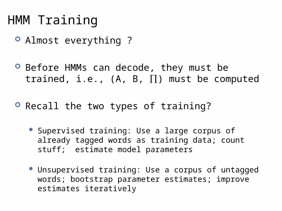
HMM Training Almost everything ?

Before HMMs can decode, they must be trained, i.e., (A, B, ∏) must be computed

Recall the two types of training?

Supervised training: Use a large corpus of already tagged words as training data; count stuff; estimate model parameters

Unsupervised training: Use a corpus of untagged words; bootstrap parameter estimates; improve estimates iteratively

Supervised Training We have training data, i.e., thousands of sentences with

their words already tagged

Given this data, we already have the set of states and symbols

Next, compute Maximum Likelihood Estimates (MLEs) for the various parameters

Those estimates of the parameters that maximize the likelihood that the training data was actually generated by our model

52

Supervised Training Transition Probabilities

Any P(ti | ti-1) = C(ti-1ti)/Σt’C(ti-1t’) from the training data For P(NN|VB), count how many times a noun follows a verb and

divide by the the number of times anything else follows a verb

Emission Probabilities Any P(wi | ti) = C(wi,ti)/Σw’C(w’, ti) from the training data For P(bank|NN), count how many times the word bank was seen

tagged as a noun and divide by the number of times anything was seen tagged as a noun

Priors The prior probability of any state (tag) For ∏noun, count the number of times a noun occurs and divide by

the total number of words in the corpus

53

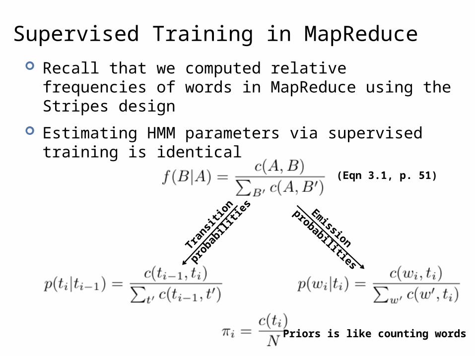
Supervised Training in MapReduce Recall that we computed relative frequencies of words in

MapReduce using the Stripes design

Estimating HMM parameters via supervised training is identical

(Eqn 3.1, p. 51)

Tran

sitio

n

pro

babili

ties Em

ission

probabilities

Priors is like counting words

Unsupervised Training No labeled/tagged training data

No way to compute MLEs directly

Make an initial guess for parameter values

Use this guess to get a better estimate

Iteratively improve the estimate until some convergence criterion is met

EXPECTATION MAXIMIZATION (EM)

Expectation Maximization A fundamental tool for unsupervised machine learning

techniques

Forms basis of state-of-the-art systems in MT, Parsing, WSD, Speech Recognition and more

Seminal paper (with a very instructive title)Maximum Likelihood from Incomplete Data via the EM algorithm, JRSS, Dempster et al., 1977

56

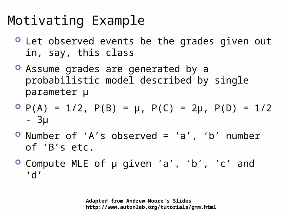
Motivating Example Let observed events be the grades given out in, say, this

class

Assume grades are generated by a probabilistic model described by single parameter μ

P(A) = 1/2, P(B) = μ, P(C) = 2μ, P(D) = 1/2 - 3μ

Number of ‘A’s observed = ‘a’, ‘b’ number of ‘B’s etc.

Compute MLE of μ given ‘a’, ‘b’, ‘c’ and ‘d’

Adapted from Andrew Moore’s Slideshttp://www.autonlab.org/tutorials/gmm.html

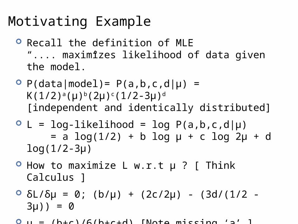
Motivating Example Recall the definition of MLE

“.... maximizes likelihood of data given the model.”

P(data|model)= P(a,b,c,d|μ) = K(1/2)a(μ)b(2μ)c(1/2-3μ)d

[independent and identically distributed]

L = log-likelihood = log P(a,b,c,d|μ) = a log(1/2) + b log μ + c log 2μ + d log(1/2-3μ)

How to maximize L w.r.t μ ? [ Think Calculus ]

δL/δμ = 0; (b/μ) + (2c/2μ) - (3d/(1/2 - 3μ)) = 0

μ = (b+c)/6(b+c+d) [Note missing ‘a’ ]

We got our answer without EM. Boring !

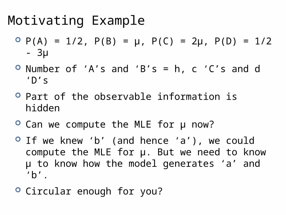
Motivating Example P(A) = 1/2, P(B) = μ, P(C) = 2μ, P(D) = 1/2 - 3μ

Number of ‘A’s and ‘B’s = h, c ‘C’s and d ‘D’s

Part of the observable information is hidden

Can we compute the MLE for μ now?

If we knew ‘b’ (and hence ‘a’), we could compute the MLE for μ. But we need to know μ to know how the model generates ‘a’ and ‘b’.

Circular enough for you?

The EM Algorithm Start with an initial guess for μ (μ0)

t = 1; Repeat bt = μ(t-1)h/(1/2 + μ(t-1))

[E-step: Compute expected value of b given μ ]

μt = (bt + c)/6(bt + c + d) [M-step: Compute MLE of μ given b ]

t = t + 1

Until some convergence criterion is met

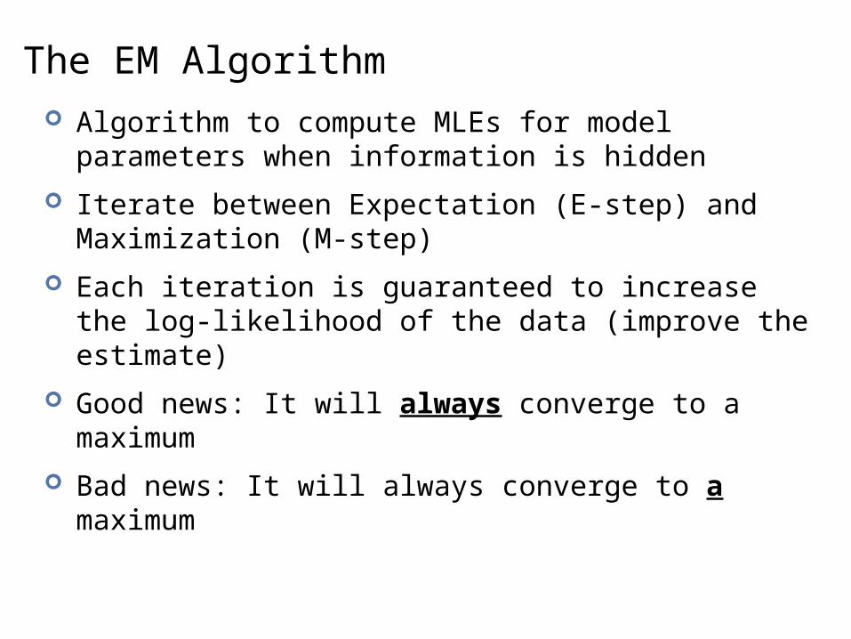
The EM Algorithm Algorithm to compute MLEs for model parameters when

information is hidden

Iterate between Expectation (E-step) and Maximization (M-step)

Each iteration is guaranteed to increase the log-likelihood of the data (improve the estimate)

Good news: It will always converge to a maximum

Bad news: It will always converge to a maximum

61

Applying EM to HMMs Just the intuition; No gory details

Hidden information (the state sequence)

Model Parameters: A, B & ∏

Introduce two new observation statistics: Number of transitions from qi to qj (ξ)

Number of times in state qi (γ)

The EM algorithm should now apply perfectly

62

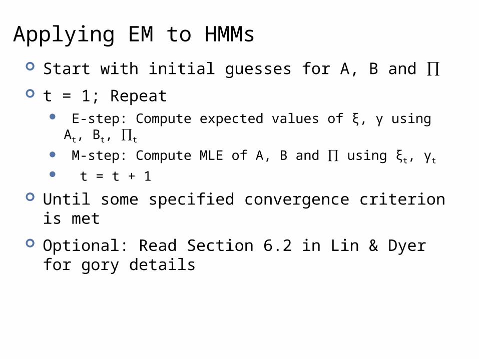
Applying EM to HMMs Start with initial guesses for A, B and ∏

t = 1; Repeat E-step: Compute expected values of ξ, γ using At, Bt, ∏t

M-step: Compute MLE of A, B and ∏ using ξt, γt

t = t + 1

Until some specified convergence criterion is met

Optional: Read Section 6.2 in Lin & Dyer for gory details

63

Baum-Welch Algorithm

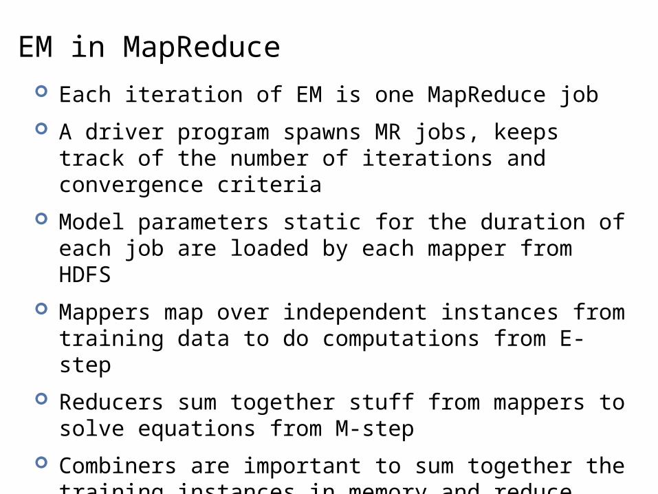
EM in MapReduce Each iteration of EM is one MapReduce job

A driver program spawns MR jobs, keeps track of the number of iterations and convergence criteria

Model parameters static for the duration of each job are loaded by each mapper from HDFS

Mappers map over independent instances from training data to do computations from E-step

Reducers sum together stuff from mappers to solve equations from M-step

Combiners are important to sum together the training instances in memory and reduce disk I/O

Source: Wikipedia (Japanese rock garden)

Questions?