1

HFEL: Joint Edge Association and Resource Allocation

for Cost-Efficient Hierarchical Federated Edge Learning

Siqi Luo, Xu Chen, Qiong Wu, Zhi Zhou, and Shuai Yu

School of Data and Computer Science, Sun Yat-sen University, Guangzhou, China

Abstract

Federated Learning (FL) has been proposed as an appealing approach to handle data privacy issue

of mobile devices compared to conventional machine learning at the remote cloud with raw user

data uploading. By leveraging edge servers as intermediaries to perform partial model aggregation

in proximity and relieve core network transmission overhead, it enables great potentials in low-latency

and energy-efficient FL. Hence we introduce a novel Hierarchical Federated Edge Learning (HFEL)

framework in which model aggregation is partially migrated to edge servers from the cloud. We further

formulate a joint computation and communication resource allocation and edge association problem for

device users under HFEL framework to achieve global cost minimization. To solve the problem, we

propose an efficient resource scheduling algorithm in the HFEL framework. It can be decomposed into

two subproblems: resource allocation given a scheduled set of devices for each edge server and edge

association of device users across all the edge servers. With the optimal policy of the convex resource

allocation subproblem for a set of devices under a single edge server, an efficient edge association

strategy can be achieved through iterative global cost reduction adjustment process, which is shown

to converge to a stable system point. Extensive performance evaluations demonstrate that our HFEL

framework outperforms the proposed benchmarks in global cost saving and achieves better training

performance compared to conventional federated learning.

Index Terms

Resource scheduling, hierarchical federated edge learning, cost efficiency.

I. INTRODUCTION

As mobile and internet of things (IoT) devices have emerged in large numbers and are gener-

ating a massive amount of data [1], Machine Learning (ML) has been witnessed to go through

a high-speed development due to big data and improving computing capacity, which prompted

arX

iv:2

002.

1134

3v2

[cs

.DC

] 6

Jun

202

0

2

the development of Artificial Intelligence (AI) to revolutionize our life [2]. The conventional ML

framework focuses on central data processing, which requires widely distributed mobile devices

to upload their local data to a remote cloud for global model training [3]. However, the cloud

server is hard to exploit such a multitude of data from massive user devices as it easily suffers

external attack and data leakage risk. Given the above threats to data privacy, many device users

are reluctant to upload their private raw data to the cloud server [4]–[6].

To tackle the data security issue in centralized training, a decentralized ML named Federated

Learning (FL) is widely envisioned as an appealing approach [7]. It enables mobile devices

collaboratively build a shared model while preserving privacy sensitive data locally from external

direct access. In the prevalent FL algorithm such as Federated Averaging (FedAvg), each mobile

device trains a model locally with its own dataset and then transmits the model parameters

to the cloud for a global aggregation [8]. With the great potential to facilitate large-scale data

collection, FL realizes model training in a distributive fashion.

Unfortunately, FL suffers from a bottleneck of communication and energy overhead before

reaching a satisfactory model accuracy due to long transmission latency in wide area network

(WAN) [9]. With devices’ limited computing and communication capacities, plethora of model

transmission rounds occur which degrades learning performance under training time budget. And

plenty of energy overhead is required for numerous computation and communication iterations

which is challenging to low battery devices. In addition, as many ML models are of large size,

directly communicating with the cloud over WAN by a massive number of device users could

worsen the congestion in backbone network, leading to significant WAN communication latency.

To mitigate such issues, we leverage the power of Mobile Edge Computing (MEC), which is

regarded as a promising distributed computing paradigm in 5G era for supporting many emerging

intelligent applications such as video streaming, smart city and augmented reality [10]. MEC

allows delay-sensitive and computation-intensive tasks to be offloaded from distributed mobile

devices to edge servers in proximity, which offers real-time response and high energy efficiency

[11]–[13]. Along this line, we propose a novel Hierarchical Federated Edge Learning (HFEL)

framework, in which edge servers usually fixedly deployed with base stations as intermediaries

between mobile devices and the cloud, can perform edge aggregations of local models which are

transmitted from devices in proximity. When each of them achieves a given learning accuracy,

updated models at the edge are transmitted to the cloud for global aggregation. Intuitively, HFEL

can help to reduce significant communication overhead over the WAN transmissions between

3

device users and the cloud via edge model aggregations. Moreover, through the coordination by

the edge servers in proximity, more efficient communication and computation resource allocation

among device users can be achieved. It can enable effective training time and energy overhead

reduction.

Nevertheless, to realize the great benefits of HFEL, we still face the following challenges:

1) how to solve a joint computation and communication resource allocation for each device to

achieve training acceleration and energy saving? The training time to converge to a predefined

accuracy level is one of the most important performance metrics of FL. While energy mini-

mization of battery-constrained devices is the main concern in MEC [13]. Both training time

and energy minimization depend on mobile devices’ computation capacities and communication

resource allocation from edge servers. As the resources of an edge server and its associated

devices are generally limited, such optimization is non-trivial to achieve. 2) How to associate

a proper set of device users to an edge server for efficient edge model aggregation? As in

Fig. 1, densely distributed mobile devices are generally able to communicate with multiple edge

servers. From the perspective of an edge server, it is better to communicate with as many mobile

devices as possible for edge model aggregation to improve learning accuracy. While more devices

choose to communicate with the same edge server, the less communication resource that each

device would get, which brings about longer communication delay. As a result, computation and

communication resource allocation for the devices and their edge association issues should be

carefully addressed to accomplish cost-efficient learning performance in HFEL.

As a thrust for the grand challenges above, in this paper we formulate a joint computation

and communication resource allocation and edge server association problem for global learning

cost minimization in HFEL. Unfortunately, such optimization problem is hard to solve. Hence

we decompose the original optimization problem into two subproblems: 1) resource allocation

problem and 2) edge association problem, and accordingly put forward an efficient integrated

scheduling algorithm for HFEL. For resource allocation, given a set of devices which are

scheduled to upload local models to the same edge server, we can solve an optimal policy,

i.e., the amount of contributed computation capacity of each device and bandwidth resource

that each device is allocated to from the edge server. Moreover, for edge association, we can

work out a feasible set of devices (i.e., a training group) for each edge server through cost

reducing iterations based on the optimal policy of resource allocation within the training group.

The iterations of edge association process finally converge to a stable system point, where each

4

Edge m

odel

uploa

ding

Global model

downloading

Edge aggregation

Cloud aggregation

Cloud 

Edge

Device

Local model

Edge model

Global model

Loca

l mod

elup

load

ing

Edge model

downloading

Local modeltraining

Fig. 1: Hierarchical Federated Edge Learning (HFEL) framework.

edge server owns a stable set of model training devices to achieve global cost efficiency and no

edge server will change its training group formation.

In a nutshell, our work makes the key contributions as follows:

• We propose a hierarchical federated edge learning (HFEL) framework which enables great

potentials in low latency and energy-efficient federated learning and formulate a holistic

joint computation and communication resource allocation and edge association model for

global learning cost minimization.

• We decompose the challenging global cost minimization problem into two subproblems:

resource allocation and edge association, and accordingly devise an efficient HFEL resource

scheduling algorithm. With the optimal policy of the convex resource allocation subproblem

given a training group of a single edge server, a feasible edge association strategy can

be solved for each edge server through cost reducing iterations which are guaranteed to

converge to a stable system point.

• Extensive numerical experiments demonstrate that our HFEL resource scheduling algorithm

is capable of achieving superior performance gain in global cost saving over comparing

5

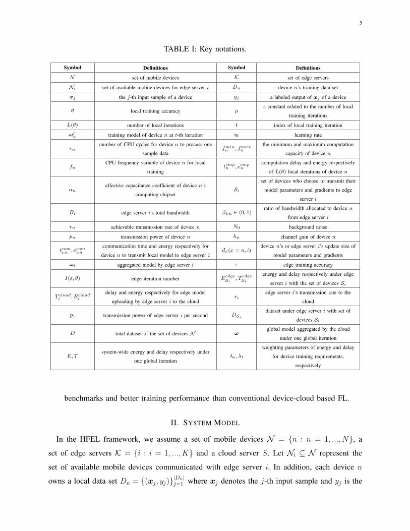
TABLE I: Key notations.

Symbol Definitions Symbol Definitions

N set of mobile devices K set of edge servers

Ni set of available mobile devices for edge server i Dn device n’s training data set

xj the j-th input sample of a device yj a labeled output of xj of a device

θ local training accuracy µa constant related to the number of local

training iterations

L(θ) number of local iterations t index of local training iteration

ωtn training model of device n at t-th iteration ηt learning rate

cnnumber of CPU cycles for device n to process one

sample datafminn , fmax

n

the minimum and maximum computation

capacity of device n

fnCPU frequency variable of device n for local

trainingtcmpn , ecmp

ncomputation delay and energy respectively

of L(θ) local iterations of device n

αneffective capacitance coefficient of device n’s

computing chipsetSi

set of devices who choose to transmit their

model parameters and gradients to edge

server i

Bi edge server i’s total bandwidth βi:n ∈ (0, 1]ratio of bandwidth allocated to device n

from edge server i

rn achievable transmission rate of device n N0 background noise

pn transmission power of device n hn channel gain of device n

tcomi:n , ecomi:n

communication time and energy respectively for

device n to transmit local model to edge server idx(x = n, i)

device n’s or edge server i’s update size of

model parameters and gradients

ωi aggregated model by edge server i ε edge training accuracy

I(ε, θ) edge iteration number EedgeSi , T edge

Sienergy and delay respectively under edge

server i with the set of devices Si

T cloudi , Ecloud

i

delay and energy respectively for edge model

uploading by edge server i to the cloudri

edge server i’s transmission rate to the

cloud

pi transmission power of edge server i per second DSidataset under edge server i with set of

devices Si

D total dataset of the set of devices N ωglobal model aggregated by the cloud

under one global iteration

E, Tsystem-wide energy and delay respectively under

one global iterationλe, λt

weighting parameters of energy and delay

for device training requirements,

respectively

benchmarks and better training performance than conventional device-cloud based FL.

II. SYSTEM MODEL

In the HFEL framework, we assume a set of mobile devices N = {n : n = 1, ..., N}, a

set of edge servers K = {i : i = 1, ..., K} and a cloud server S. Let Ni ⊆ N represent the

set of available mobile devices communicated with edge server i. In addition, each device n

owns a local data set Dn = {(xj, yj)}|Dn|j=1 where xj denotes the j-th input sample and yj is the

6

corresponding labeled output of xj for n’s federated learning task. The key notations used in

this paper are summarized in Table I.

A. Learning process in HFEL

We consider our HFEL architecture as Fig. 1, in which one training model goes through

model aggregation in edge layer and cloud layer. Therefore, the shared model parameters by

mobile devices in a global iteration involve edge aggregation and cloud aggregation. To quantify

training overhead in the HFEL framework, we formulate energy and delay overheads in edge

aggregation and cloud aggregation within one global iteration. Note that in most FL scenarios,

mobile devices participate in collaborative learning when they are in static conditions such as

in the battery-charging state. Hence we assume that in the HFEL architecture, devices remain

stable in the learning process, during which their geographical locations keep almost unchanged.

1) Edge Aggregation: At this stage, it includes three steps: local model computation, local

model transmission and edge model aggregation. That is, local models are first trained by mobile

devices and then transmitted to their associated edge servers for edge aggregation, which can

be elaborated as the following steps.

Step 1. Local model computation. At this step for a device n, it needs to solve the

machine learning model parameter ω which characterizes each output value yj with loss function

fn(xj, yj,ω). The loss function on the data set of device n is defined as

Fn(ω) =1

|Dn|

|Dn|∑j=1

fn(xj, yj,ω). (1)

To achieve a local accuracy θ ∈ (0, 1) which is common to all the devices for a same model,

device n needs to run a number of local iterations formulated as L(θ) = µ log (1/θ) for a wide

range of iterative algorithms [14]. Constant µ depends on the data size and the machine learning

task. At t-th local iteration, each device n’s task is to figure out its local update as

ωtn = ωtn − η∇Fn(ωt−1n ), (2)

until ||∇Fn(ωtn)|| ≤ θ||∇Fn(ωt−1n )|| and η is the predefined learning rate [15].

Accordingly, the formulation of computation delay and energy overheads incurred by device

n can be given in the following. Let cn be the number of CPU cycles for device n to process one

sample data. Considering that each sample (xj, yj) has the same size, the total number of CPU

cycles to run one local iteration is cn|Dn|. We denote the allocated CPU frequency of device n

7

for computation by fn with fn ∈ [fminn , fmaxn ]. Thus the total delay of L(θ) local iterations of n

can be formulated as

tcmpn = L(θ)cn|Dn|fn

, (3)

and the energy cost of the total L(θ) local iterations incurred by device n can be given as [16]

ecmpn = L(θ)αn2f 2ncn|Dn|, (4)

where αn/2 represents the effective capacitance coefficient of device n’s computing chipset.

Step 2. Local model transmission. After finishing L(θ) local iterations, each device n

will transmit its local model parameters ωtn to a selected edge server i, which incurs wireless

transmission delay and energy. Then for an edge server i, we characterize the set of devices who

choose to transmit their model parameters to i as Si ⊆ Ni.

In this work, we consider an orthogonal frequency-division multiple access (OFDMA) protocol

for devices in which edge server i provides a total bandwidth Bi. Define βi:n as the bandwidth

allocation ratio for device n such that i’s resulting allocated bandwidth is βi:nBi. Let rn denote

the achievable transmission rate of device n which is defined as

rn = βi:nBi ln (1 +hnpnN0

), (5)

where N0 is the background noise, pn is the transmission power, and hn is the channel gain of

device n (which is referred to [17]). Let tcomi:n denote the communication time for device n to

transmit ωtn to edge server i and dn denote the data size of model parameters ωtn. Thus tcomi:n can

be characterized by

tcomi:n = dn/rn. (6)

Given the communication time and transmission power of n, the energy cost of n to transmit

dn is

ecomi:n = tcomi:n pn =dnpn

βi:nBi ln (1 + hnpnN0

). (7)

Step 3. Edge model aggregation. At this step, each edge server i receives the updated model

parameters from its connected devices Si and then averages them as

ωi =

∑n∈Si |Dn|ωtn|DSi|

, (8)

where DSi = ∪n∈SiDn is aggregated data set under edge server i.

8

After that, edge server i broadcasts ωi to its devices in Si for the next round of local model

computation (i.e. step 1). In other words, step 1 to step 3 of edge aggregation will iterate until

edge server i reaches an edge accuracy ε which is the same for all the edge servers. We can

observe that each edge server i won’t access the local data Dn of each device n, thus preserving

personal data privacy. In order to achieve the required model accuracy, for a general convex

machine learning task, the number of edge iterations is shown to be [18]

I(ε, θ) =δ(log (1/ε))

1− θ, (9)

where δ is some constant that depends on the learning task. Note that our analysis framework

can also be applied when the relation between the convergence iterations and model accuracy is

known in non-convex learning tasks.

Since an edge server typically has strong computing capability and stable energy supply, the

edge model aggregation time and energy cost for broadcasting the aggregated model parameter

ωi is not considered in our optimization model. Since the time and energy cost for a device

receiving edge aggregated model parameter ωi is small compared to uploading local model

parameters, and keeps almost constant during each iteration, we also ignore this part in our

model. Thus, after I(ε, θ) edge iterations, the total energy cost of edge server i’s training group

Si is given by

EedgeSi =

∑n∈Si

I(ε, θ)(ecomi:n + ecmpn ). (10)

Similarly, the delay including computation and communication for edge server i to achieve an

edge accuracy ε can be derived as

T edgeSi = I(ε, θ) maxn∈Si{tcomi:n + tcmpn }. (11)

From (11), we notice that the bottleneck of the computation delay is affected by the last device

who finishes all the local iterations, while the communication delay bottleneck is determined by

the device who spends the longest time in model transmission after local training.

2) Cloud Aggregation: At this stage, we have two steps: edge model uploading and cloud

model aggregation. That is, each edge server i ∈ K uploads ωi to the cloud for global aggregation

after I(ε, θ) times edge aggregation.

Step 1. Edge model uploading. Let ri denote the edge server i’s transmission rate to the

remote cloud for edge model uploading, pi the transmission power per sec and di the edge server

9

i’s model parameter size. We then derive the delay and energy for edge model uploading by

edge server i respectively as

T cloudi =diri, (12)

Ecloudi = piT

cloudi . (13)

Step 2. Cloud model aggregation. At this final step, the remote cloud receives the updated

models from all the edge servers and aggregates them as:

ω =

∑i∈K |DSi |ωi|D|

, (14)

where D = ∪i∈KDSi .

As a result, neglecting the aggregation time at cloud which is much smaller than that on the

mobile devices, we can obtain the system-wide energy and delay under one global iteration as

E =∑i∈K

(Ecloudi + Eedge

Si ), (15)

T = maxi∈K{T cloudi + T edgeSi }. (16)

For a more clear description, we provide one global aggregation iteration procedure of HFEL in

Algorithm 1. Such global aggregation procedure can be repeated by pushing the global model

parameter ω to all the devices via the edge servers, until the stopping condition (e.g., the model

accuracy or total training time) is satisfied.

B. Problem Formulation

Given the system model above, we now consider the system-wide performance optimization

with respect to energy and delay minimization within one global iteration. Let λe, λt ∈ [0, 1]

represent the importance weighting indicators of energy and delay for the training objectives,

respectively. Then the HEFL optimization problem is formulated as follows:

min λeE + λtT, (17)

subject to,∑n∈Si

βi:n ≤ 1,∀i ∈ K, (17a)

0 < βi:n ≤ 1,∀n ∈ Si,∀i ∈ K, (17b)

fminn ≤ fn ≤ fmaxn ,∀n ∈ N , (17c)

10

Algorithm 1 HFEL under one global iteration

Input: Initial models of all the devices {ω0n∈N} with local iteration t = 0, local accuracy θ,

edge accuracy ε;

Output: Global model ω;

1:

2: Edge aggregation:

3: for t = 1, 2, ..., I(ε, θ)L(θ) do

4: for each device n = 1, ..., N in parallel do

5: n solves local problem (2) and derives ωtn. (Local model computation)

6: end for

7: All the devices transmit their updated ωtn to edge server i. (Local model transmission)

8:

9: if t % L(θ) = 0 then

10: for each edge server i = 1, ..., K in parallel do

11: i calculates (8) after receiving {ωtn : n ∈ Si}, and obtains ωi. (Edge model

aggregation)

12: i broadcasts ωi to Si such that ωtn = ωi,∀n ∈ Si.

13: end for

14: end if

15: end for

16:

17: Cloud aggregation:

18: After receiving {ωi∈K}, the cloud solves problem (14) and derives the global model ω.

Si ⊆ Ni,∀i ∈ K, (17d)

∪i∈K Si = N , (17e)

Si ∩ Sk = ∅, ∀i, k ∈ K and i 6= k, (17f)

where (17a) and (17c) respectively represent the uplink communication resource constraints and

computation capacity constraints, (17d) and (17e) ensure all the devices in the system participate

in the model training, and (17f) requires that each device is allowed to associate with one edge

11

Initial resourcescheduling

Each device nperforms permitted

transferringadjustment

Solve optimalresource allocaitonunder single edge

serverEach pair of device n,m performs permitted

exchangingadjustment

if any device has permitted 

adjustment?

Yes

No

Finish

Updated edge association

Improved resource allocation

Edge association

Resource allocation

Fig. 2: Basic procedure of HFEL scheduling policy.

server for model parameter uploading and aggregation for sake of cost saving.

Unfortunately, this optimization problem is hard to solve due to the large combinatorial search

space of the edge association decision constraints (17d)-(17f) and their coupling with computation

and communication resource allocation in the objective function. This implies that for large inputs

it is impractical to obtain the global optimal solution in a real-time manner. Thus, efficient

approximating algorithm with low-complexity is highly desirable and this motivates the HFEL

scheduling algorithm design in the following.

C. Overview of HFEL Scheduling Scheme

Since the optimization problem (17) is hard to solve directly, a common and intuitive solution

is to design a feasible and computation efficient approach to approximately minimize the system

cost. Here we adopt the divide-and-conquer principle and decompose the HFEL scheduling

algorithm design issue into two key subproblems: resource allocation within a single edge server

and edge association across multiple edge servers.

As shown in Fig. 2, the basic procedures of our scheme are elaborated as follows:

12

• We first carry out an initial edge association strategy (e.g., each device connects to its

closest edge server). Given the initial edge association strategy, we then solve the optimal

resource allocation for the devices within each edge sever (which is given in Section III

later on).

• Then we define that for each device, it has two possible adjustments to perform to improve

edge association scheme: transferring or exchanging (which will be formally defined in

Section IV later on). These adjustments are permitted to carry out if they can improve the

system-wide performance without damaging any edge server’s utility.

• When a device performs a permitted adjustment, it incurs a change of systematic edge

association strategy. Thus we will work out the optimal resource allocation for each edge

server with updated edge association.

• All the devices iteratively perform possible adjustments until there exists no permitted

adjustment, i.e., no change of systematic edge association strategy.

As shown in the following sections, the resource allocation subproblem can be efficiently

solved in practice using convex optimization solvers, and the edge association process can

converge to a stable point within a limited number of iterations. Hence the resource scheduling

algorithm for HFEL can converge in a fast manner and is amendable for practical implementation.

III. OPTIMAL RESOURCE ALLOCATION WITHIN SINGLE EDGE SERVER

In this section, we concentrate on the optimal overhead minimization within a single edge

server, i.e., considering joint computation and communication resource allocation subproblem

under edge server i given scheduled training group of devices Si.To simplify the notations, we first introduce the following terms:

An =λeI(ε, θ)dnpn

Bi ln (1 + hnpnN0

),

Bn =λeI(ε, θ)L(θ)αn2cn|Dn|,

W =λtI(ε, θ),

Dn =dn

Bi ln (1 + hnpnN0

),

En =L(θ)cn|Dn|,

where An, Bn, Dn, En and W are constants related to device n’s parameters and system setting.

Then through refining and simplifying the aforementioned formulation (17) in a single edge server

13

scenario, we can derive a subproblem formulation of edge server i’s overhead minimization under

one global iteration as follows:

min Ci =λeEedgeSi (fn, βi:n) + λtT

edgeSi (fn, βi:n) (18)

=∑n∈Si

(Anβi:n

+Bnf2n) +W max

n∈Si{Dn

βi:n+Enfn},

subject to,

0 <∑n∈Si

βi:n ≤ 1, (18a)

fminn ≤ fn ≤ fmaxn ,∀n ∈ Si, (18b)

0 < βi:n ≤ 1,∀n ∈ Si. (18c)

For the optimization problem (18), we can show it is a convex optimization problem as stated

in the following.

Theorem 1: The resource allocation subproblem (18) is convex.

Proof. The subformulas of Ci consist of three parts: 1) An

βi:n, 2) Bnf

2n and 3) maxn∈Si{ Dn

βi:n+ En

fn},

each of which is intuitively convex in its domain and all constraints get affine such that problem

(18) is convex. �

By exploiting the Karush-Kuhn-Tucker (KKT) conditions of problem (18), we can obtain the

following structural result.

Theorem 2: The optimal solutions to device n’s bandwidth and computation capacity alloca-

tions β∗i:n and f ∗n under edge server i of (18) satisfy

β∗i:n =(An + 2Bnf∗3n

EnDn)

13∑

n∈Si(An + 2Bnf∗3n

EnDn)

13

. (19)

Proof. First to make (18) better tractable, let t = maxn∈Si{ Dn

βi:n+ En

fn} and t ≥ Dn

βi:n+ En

fn,∀n ∈ Si.

Then problem (18) can be further transformed to

min Ci =∑n∈Si

(Anβi:n

+Bnf2n) +Wt, (20)

subject to,∑n∈Si

βi:n ≤ 1, (20a)

fminn ≤ fn ≤ fmaxn ,∀n ∈ Si, (20b)

14

Algorithm 2 Resource Allocation Algorithm

Input: Initial {fn : n ∈ Si} by random setting;

Output: Optimal resource allocation policy under edge server i as {β∗i:n : n ∈ Si} and {f ∗n :

n ∈ Si}.

1: Replace βi:n with equation (19) in problem (18), which then is transformed to an equivalent

convex optimization problem (32) with respective to variables {fn : n ∈ Si}.

2: Utilize convex optimization solvers (e.g., CVX and IPOPT) to solve (32) and obtain

optimal computation capacity allocation {f ∗n : n ∈ Si}.

3: Given {f ∗n : n ∈ Si}, optimal bandwidth allocation {β∗i:n : n ∈ Si} can be derived based

on (19).

0 < βi:n ≤ 1,∀n ∈ Si, (20c)

Dn

βi:n+Enfn≤ t,∀n ∈ Si. (20d)

Given Si,∀i ∈ K, problem (20) is convex such that it can be solved by the Lagrange multiplier

method. The partial Lagrange formula can be expressed as

Li =∑n∈Si

(Anβi:n

+Bnf2n) +Wt+ φ(

∑n∈Si

βi:n − 1) +∑n∈Si

τn(Dn

βi:n+Enfn− t),

where φ and τn are the Lagrange multipliers related to constraints (20a) and (20d). Applying

KKT conditions, we can derive the necessary and sufficient conditions in the following.

∂L

∂βi:n= φβi:n −

An + τnDn

β2i:n

= 0,∀n ∈ Si, (21)

∂L

∂fn= 2Bnfn −

τnEnf 2n

= 0, ∀n ∈ Si, (22)

∂L

∂t= W −

∑n∈Si

τn = 0,∀n ∈ Si, (23)

φ(∑n∈Si

βi:n − 1) = 0, φ ≥ 0, (24)

τn(Dn

βi:n+Enfn− t) = 0, τn ≥ 0,∀n ∈ Si, (25)

fminn ≤ fn ≤ fmaxn , 0 < βi:n ≤ 1,∀n ∈ Si. (26)

From (21) and (22), we can derive the relations below:

φ =An + τnDn

β3i:n

> 0, (27)

15

βi:n = (An + τnDn

φ)13 , (28)

τn =2Bnf

3n

En, (29)

based on which, another relation expression can be obtained combining (24) as follows.∑n∈Si

(An + τnDn)13 = φ

13 =

(An + τnDn)13

βi:n. (30)

Hence, we can easily work out

βi:n =(An + τnDn)

13∑

n∈Si (An + τnDn)13

. (31)

Finally, replacing τn with (29) in expression (31), the optimal bandwidth ratio β∗i:n can be easily

figured out as (19). �

Given the conclusions in Theorem 1 and 2, we are able to efficiently solve the resource

allocation problem (18) with Algorithm 2. Likewise, by replacing βi:n with (19), we can transform

problem (18) to an equivalent convex optimization problem as

min∑n∈Si

(An

∑n∈Si (An + 2Bnf3n

EnDn)

13

(An + 2Bnf3nEn

Dn)13

+Bnf2n)+

W maxn∈Si{Dn

∑n∈Si (An + 2Bnf3n

EnDn)

13

(An + 2Bnf3nEn

Dn)13

+Enfn}, (32)

subject to,

fminn ≤ fn ≤ fmaxn ,∀n ∈ Si. (33)

Since the original problem (18) is convex and βi:n is convex with respect to fn, the transformed

problem (32) above is also convex, which can be solved by some convex optimization solvers

(e.g., CVX and IPOPT) to obtain optimal solution {f ∗n : n ∈ Si}. After that, optimal solution

{β∗i:n : n ∈ Si} can be derived based on (19) given {f ∗n : n ∈ Si}. Note that by such problem

transformation, we can greatly reduce the size of decision variables in the original problem (18)

which can help to significantly reduce the solution computing time in practice.

IV. EDGE ASSOCIATION FOR MULTIPLE EDGE SERVERS

We then consider the edge association subproblem for multiple edge servers. Given the optimal

resource allocation of scheduled devices under a single edge server, the key idea of solving

16

systematic overhead minimization is to efficiently allocate a bunch of devices to each edge

server for edge model aggregation. In the following, we will design an efficient edge association

for all the edge servers, in order to iteratively improve the overall system performance.

First we introduce some critical concepts and definitions about edge association by each edge

server in the following.

Definition 1: In our system, a local training group Si is termed as a subset of Ni, in

which devices choose to upload their local models to edge server i for edge aggregation.

Correspondingly, the utility of Si can be derived as v(Si) = −Ci(f ∗,β∗i ) which takes a minus

sign over the minimum cost of solving resource allocation subproblem for edge server i.

Definition 2: An edge association strategy DS = {Si : i ∈ K} is defined as the set of local

training groups of all the edge servers, where Si = {n : n ∈ Ni}, such that the system-wide

utility given scheduled DS can be denoted as v(DS) =∑K

i=1 v(Si).

For the whole system, which kind of edge association strategy it prefers depends on v(DS).

To compare different edge association strategies, we define a preference order based on v(DS)

which reflects preferences of all the edge servers for different local training group formations.

Definition 3: Given two different edge association strategies DS1 and DS2, we define a

preference order as DS1 B DS2 if and only if v(DS1) > v(DS2). It indicates that edge

association strategy DS1 is preferred over DS2 to gain lower overhead by all the edge servers.

Next, we can solve the overhead minimization problem by constantly adjusting edge associ-

ation strategy DS, i.e., each edge server’s training group formation, to gain lower overhead in

accordance with preference order B. The edge association adjusting will result in termination

with a stable DS∗ where no edge server i in the system will deviate its local training group

from S∗i ∈ DS∗.

Obviously the adjustment of edge association strategy DS basically results from the change

of each edge server’s local training group formation. In our system, it is permitted to perform

some edge association adjustments with utility improvement based on B defined as follows.

Definition 4: A device transferring adjustment by n means that device n ∈ Si with |Si| > 2

retreats its current training group Si and joins another training group S−i. Causing a change from

DS1 to DS2, the device transferring adjustment is permitted if and only if DS2 B DS1.

Definition 5: A device exchanging adjustment between edge servers i and j means that

device n ∈ Si and m ∈ Sj are switched to each other’s local training group. Causing a change

from DS1 to DS2, the device exchanging adjustment is permitted if and only if DS2 B DS1.

17

Based on the wireless communication between devices and edge servers, each device reports

all its detailed information (including computing and communication parameters) to its available

edge servers. Then each edge server i will calculate its own utility v(Si), communicate with the

other edge servers through cellular links and manage the edge association adjustments.

With the iteration of every permitted adjustment which brings a systematic overhead decrease

by ∆ = v(DS2)− v(DS1), the edge association adjustment process will terminate to be stable

where no edge server will deviate from the current edge association strategy.

Definition 6: An edge association strategy DS∗ is at a stable system point if no edge server

i will change S∗i ∈ DS∗ to obtain lower global training overhead with S∗−i ∈ DS∗ unchanged.

That is, at a stable system point DS∗, no edge server i will deviate its local training group

formation from S∗i ∈ DS∗ to achieve lower global FL overhead given optimal resource allocation

within S∗i .

Next, we devise an edge association algorithm to achieve cost efficiency in HFEL for all

the edge servers and seek feasible computation and communication resource allocation for their

training groups. Note that in our scenario, each edge server has perfect knowledge of the channel

gains and computation capacities of its local training group which can be obtained by feedback.

They also can connect with each other through cellular links. Thus, our decentralized edge

association process is implemented by all the edge servers, which consists of two steps: initialized

allocation and edge association as described in Algorithm 3.

In the first stage, initialization allocation procedure is as follows.

• First for each edge server i ∈ K, local training group Si is randomly formed.

• Then given Si, edge server i solves resource allocation subproblem, i.e., obtaining f ∗n and

β∗i:n,∀n ∈ Si and deriving v(Si).

• After the initial edge associations of all the edge servers complete, an initial edge association

strategy DS = {Si, ...,SK} can be achieved.

In the second stage, edge servers execute edge association by conducting permitted edge

association adjustments in an iterative way until no local training group will be changed. At

each iteration, edge servers involved will calculate their own utilities. Specially, a historical

group set hi is maintained for each edge server i to record the group composition it has formed

before with the corresponding utility value so that repeated calculations can be avoided.

Take device transferring adjustment for example. During an iteration, an edge server i firstly

contends to conduct device transferring adjustment. That is, edge server i transfers its device n

18

Algorithm 3 Edge Association AlgorithmInput: Set of devices N , tasks T and sensing data K;

Output: Stable system point DS∗.

1: for i = 1 to K do

2: edge server i randomly forms Si.

3: i solves optimal resource allocation and derives an initial v(Si) within Si.

4: end for

5: An initial edge association strategy is obtained as DS.

6:

7: repeat

8: for n = 1 to N do

9: each pair of edge server i and j with i 6= j perform device transferring adjustment

by transferring device n (n ∈ Si and n ∈ Nj) from Si to Sj if permitted. Then hi and hj

are accordingly updated.

10: end for

11: randomly pick device n ∈ Si and m ∈ Sj where i 6= j, perform device exchanging

adjustment if permitted. Then hi, hj and DS are accordingly updated.

12: until no edge association adjustment is permitted by any device n ∈ N .

13:

14: Obtain the optimal edge association DS∗ with each Si ∈ DS∗ achieving f ∗n and β∗i:n, n ∈ Si.

from Si to another edge server j’s training group Sj . And we define S ′i = Si\n and S ′j = Sj∪{n}.

This leads to a change of edge association strategy from DS1 to DS2. Secondly, note that each

edge server i maintains a historical set hi to record the group composition it has formed before

with the corresponding utility value. It enables edge server i and j to reckon their utility changes

as ∆i = v(S ′i) − v(Si) and ∆j = v(S ′j) − v(Sj), which can also reflect the system-wide utility

improvement ∆ = ∆i + ∆j = v(DS2) − v(DS1). Finally, edge server i and j can decide to

conduct this device transferring adjustment when ∆ > 0.

After the edge association algorithm converges, all the involved mobile devices will execute

local training with the optimal resource allocation strategy f ∗n and β∗i:n that are broadcast from

the edge server.

19

Extensive performance evaluation in Section V shows that the proposed edge association

algorithm can converge in a fast manner, with an almost linear convergence speed.

V. PERFORMANCE EVALUATION

In this section, we carry out simulations to evaluate: 1) the global cost saving performance of

the proposed resource scheduling algorithm and 2) HFEL performance in terms of test accuracy,

training accuracy and training loss. From the perspective of devices’ and edge servers’ availabil-

ity, all the devices and edge servers are distributed randomly within an entire 500M × 500M

area.

TABLE II: Simulation settings.

Parameter Value

Maximum Bandwidth of Edge Servers 10 MHz

Device Transmission Power 200 mW

Device CPU Freq. [1, 10] GHz

Device CPU Power 600 mW

Processing Density of Learning Tasks [30, 100] cycle/bit

Background Noise 10−8 W

Device Training Size [5, 10] MB

Updated Model Size 25000 nats

Capacitance Coefficient 2× 10−28

Learning rate 0.0001

A. Performance gain in cost reduction

Typical parameters of devices and edge servers are provided in Table II with image classifi-

cation learning tasks on a dataset MNIST [20]. To characterize mobile device heterogeneity for

MNIST dataset, we have each device maintain only two labels over the total of 10 labels and

their sample sizes are different based on the law power in [21]. Furthermore, each device trains

with full batch size. Under varying device number from 15 to 60 and edge server number from

5 to 25, we compare our algorithm to the following schemes to present the performance gain in

cost reduction with local training accuracy θ = 0.9 and edge training accuracy ε = 0.9:

• Random edge association: each edge server i selects the set of mobile devices Si in a random

way and then solves the optimal resource allocation for Si. That is, it only optimizes resource

allocation subproblem given a set of devices.

20

• Greedy edge association: each device can select the connected edge server sequentially

based on the geographical distance to each edge server in an ascending order. After that, each

edge server i solves the optimal resource allocation with Si. It also only optimizes resource

allocation subproblem without edge association similar to random resource allocation.

• Computation optimization: in this scheme, resource allocation subproblem for each Si, i ∈ K

solves optimal computation capacity f ∗n∈Si given evenly distribution of bandwidth ratio.

• Communication optimization: in this scheme, resource allocation subproblem for each Si, i ∈

K solves optimal bandwidth ratio allocation β∗i:n with random computation capacity decision

fn∈Si ∈ [fminn , fmaxn ].

• Uniform resource allocation: in this scheme, we leverage the same edge association strategy

as our proposed algorithm. While in the resource allocation subproblem, the bandwidth of

each edge server i is evenly distributed to mobile devices in Si and the computation capacity

of n ∈ Si is randomly determined between fminn and fmaxn . That is, edge association

subproblem is solved without resource allocation optimization.

• Proportional resource allocation: for all the edge servers, we as well adopt edge association

strategy to improve {Si : i ∈ K}. While in the resource allocation subproblem, the

bandwidth of each edge server i is distributed to each n ∈ Si reversely proportional

to the distance li,n such that communication bottle can be mitigated. Similarly, random

computation capacity decision of n is fn∈Si ∈ [fminn , fmaxn ]. Similar to uniform resource

allocation, only edge association subproblem is solved.

As presented in Fig. 3 to Fig. 8 in which uniform resource allocation is regarded as benchmark,

our HFEL algorithm achieves the lowest global energy ratio, learning delay ratio and global cost

ratio compared to the proposed schemes.

First we explore the impact of different device numbers on the performance gain in cost

reduction by fixing edge server number as 5 in Fig. 3 to Fig. 5. Under the weights of energy

and delay as λe = 0 and λt = 1 in Fig. 3, HFEL algorithm accomplishes a satisfying learning

delay ratio as 63.3%, 46.2%, 43.3%, 56.0% and 44.4% compared to uniform resource allocation

as device number grows. Similarly in Fig. 4 with energy and delay weights as λe = 1 and λt = 0,

our HFEL scheme achieves global energy cost ratio as 30% at most compared to uniform resource

allocation and 5.0% compared to computation optimization scheme. As described in Fig. 5 in

which weights of time and energy are randomly assigned, i.e., λe, λt ∈ [0, 1] and λe + λt = 1, it

shows that HFEL algorithm still outperforms the other six schemes. Compared to computation

21

15 20 30 45 60Device number

0

25

50

75

100

125

150

175

200

Lear

ning

del

ay ra

tio (%

)HFEL resource schedulingComputation optimizationGreedy edge associationRandom edge associationCommunication optimizationProportional resource allcationUniform resource allocation

Fig. 3: Learning delay ratio

under growing device number.

15 20 30 45 60Device number

0

25

50

75

100

125

150

175

Glob

al e

nerg

y co

st ra

tio (%

)

HFEL resource schedulingComputation optimizationGreedy edge associationRandom edge associationCommunication optimizationProportional resource allcationUniform resource allocation

Fig. 4: Global energy ratio

under growing device number.

15 20 30 45 60Device number

0

25

50

75

100

125

150

175

Glob

al c

ost r

atio

(%)

HFEL resource schedulingComputation optimizationGreedy edge associationRandom edge associationCommunication optimizationProportional resource allcationUniform resource allocation

Fig. 5: Global cost ratio under

growing device number.

5 10 15 20 25Server number

0

25

50

75

100

125

150

175

200

Lear

ning

del

ay ra

tio (%

)

HFEL resource schedulingComputation optimizationGreedy edge associationRandom edge associationCommunication optimizationProportional resource allcationUniform resource allocation

Fig. 6: Learning delay ratio

under growing server number.

5 10 15 20 25Server number

0

25

50

75

100

125

150

175

200

Glob

al e

nerg

y co

st ra

tio (%

)

HFEL resource schedulingComputation optimizationGreedy edge associationRandom edge associationCommunication optimizationProportional resource allcationUniform resource allocation

Fig. 7: Global energy ratio

under growing server number.

5 10 15 20 25Server number

0

25

50

75

100

125

150

175

200

Glob

al c

ost r

atio

(%)

HFEL resource schedulingComputation optimizationGreedy edge associationRandom edge associationCommunication optimizationProportional resource allcationUniform resource allocation

Fig. 8: Global cost ratio under

growing server number.

optimization, greedy device allocation, random device allocation, communication optimization,

proportional resource allocation and uniform resource allocation schemes, our algorithm is more

efficient and fulfills up to 10%, 14.0%, 20.0%, 51.2%, 61.5% and 57.7% performance gain in

global cost reduction, respectively.

Then with device number fixed as 60, Fig. 6 to Fig. 8 exhibit that our HFEL algorithm

still has better performance gain than the other comparing schemes. For example, compared to

uniform resource allocation scheme, the HFEL scheme obtains the highest learning delay ratio

as 51.6% in Fig. 6 and the highest global energy cost ratio as 50.0% in Fig. 7. Meanwhile, Fig.

8 presents that our HFEL algorithm can achieve up to 5.0%, 25.0%, 24.0%, 28.0% and 40.3%

global cost reduction ratio over computation optimization, greedy device allocation, random

device allocation, communication optimization and proportional resource allocation schemes,

respectively.

It is interesting to find that the performance gain of our HFEL scheme compared to the

benchmark in global energy ratios as Fig. 4 and Fig. 7 is better than that in learning delay

22

20 30 40 50 60Device number

30

40

50

60

70

80

90

100

110Co

st re

ducin

g ite

ratio

n nu

mbe

r

Fig. 9: Cost reducing iteration number under

growing devices.

5 10 15 20 25Edge server number

120

140

160

180

200

Cost

redu

cing

itera

tion

num

ber

Fig. 10: Cost reducing iteration number under

growing servers.

ratios shown in Fig. 3 and Fig. 6. That is because in the objective function, the numerical value

of energy cost is much larger than the value of learning delay, which implies that the energy

weight plays a leading role in global cost reduction. Note that greedy device allocation and

random device allocation schemes only optimize resource allocation subproblem without edge

association. While proportional resource allocation and uniform resource allocation strategies

solve edge association without resource allocation optimization. It can be figured out that the

performance gain of resource allocation optimization in global cost reduction greatly dominates

that of edge association solution.

Further, we show the average iteration number of our algorithm in Fig. 9 with growing number

of devices from 15 to 60, and the average iteration number of our algorithm in Fig. 10 with the

number of edge servers ranging from 5 to 25. The results show that the convergence speed of the

proposed edge association strategy is fast and grows (almost) linearly as the numbers of mobile

device and edge server increase, which reflects the computation efficiency of edge association

algorithm.

B. Performance gain in training loss and accuracy

In this subsection setting, the performance of HFEL is validated on dataset MNIST [20] and

FEMNIST [22] (an extended MNIST dataset with 62 labels which is partitioned based on the

device of the digit or character) compared to the classic FedAvg algorithm [8]. In addition

23

0 200 400 600 800 1000Number of Global Iterations

0.80

0.82

0.84

0.86

0.88

0.90

0.92

0.94

Test

Acc

urac

y

fedhfelfedavg

(a) Test accuracy.0 200 400 600 800 1000

Number of Global Iterations0.750

0.775

0.800

0.825

0.850

0.875

0.900

0.925

0.950

Trai

ning

Acc

urac

y

fedhfelfedavg

(b) Training accuracy.

0 200 400 600 800 1000Number of Global Iterations

0.3

0.4

0.5

0.6

0.7

0.8

0.9

1.0

Trai

ning

Los

s

fedhfelfedavg

(c) Training loss.

Fig. 11: Training results under MNIST.

0 200 400 600 800 1000Number of Global Iterations

0.0

0.1

0.2

0.3

0.4

0.5

0.6

Test

Acc

urac

y

fedhfelfedavg

(a) Test accuracy.0 200 400 600 800 1000

Number of Global Iterations

0.0

0.1

0.2

0.3

0.4

0.5

0.6

Trai

ning

Acc

urac

y

fedhfelfedavg

(b) Training accuracy.

0 200 400 600 800 1000Number of Global Iterations

2.2

2.3

2.4

2.5

2.6

2.7

2.8

2.9

3.0

Trai

ning

Los

s

fedhfelfedavg

(c) Training loss.

Fig. 12: Training results under FEMNIST.

to different numbers of labels in devices for training on MNIST and FEMNIST dataset, the

number of samples of each device varies in different datasets. Specifically, for MNIST and

FEMNIST dataset, the number of data samples are in the ranges of [15,4492] and [184,334]

in each device [15], respectively. Moreover, each device trains with full batch size on both

MNIST and FEMNIST to perform image classification tasks, which utilize logistic regression

with cross-entropy loss function.

We perform training experiments to show the advantages of HFEL scheme over FedAvg,

a traditional device-cloud FL architecture not involving edge servers or resource allocation

optimization [8]. We consider 5 edge servers and 30 devices participating in the training process

for experiment. All the datasets are split with 75% for training and 25% for testing in a random

way. In the training process, 1000 global iterations are executed during each of which all the

devices go through the same number of local iterations in both HFEL and FedAvg schemes.

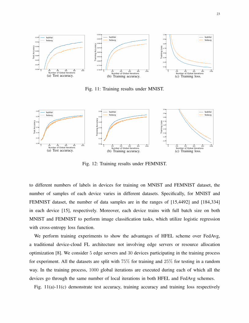
Fig. 11(a)-11(c) demonstrate test accuracy, training accuracy and training loss respectively

24

on MNIST dataset as global iteration grows. As is shown, our HFEL algorithm has higher

test accuracy and training accuracy than FedAvg both by around 5%. And HFEL has lower

training loss than FedAvg by around 3%. That is for the fact that based on the same number

of local iterations during one global iteration, devices in HFEL additionally undergo several

rounds of model aggregation in edge servers such that they benefit from model updates at the

edge. However for the devices in FedAvg, they only train with local datasets without receiving

information from external network for learning improvement during a global iteration.

Fig. 12(a)-12(c) present the training performance on dataset FEMNIST. Compared to FedAvg,

the increments in terms of test accuracy and training accuracy of HFEL under FEMNIST are

up to 4.4% and 4.0% respectively. While the reduction of training loss of HFEL compared with

FedAvg under FEMNIST is around 4.1%. Because of larger number of data samples in each

device and less number of labels to learn for MNIST than FEMNIST, HFEL reveals a higher

accuracy and lower training loss on MNIST than FEMNIST dataset in Fig. 11 and Fig. 12.

Hence it can be assumed that due to the characteristics naturally capturing device heterogeneity,

FEMNIST dataset generated by partitioning data based on MNIST would generally obtain a

worse learning performance than MNIST.

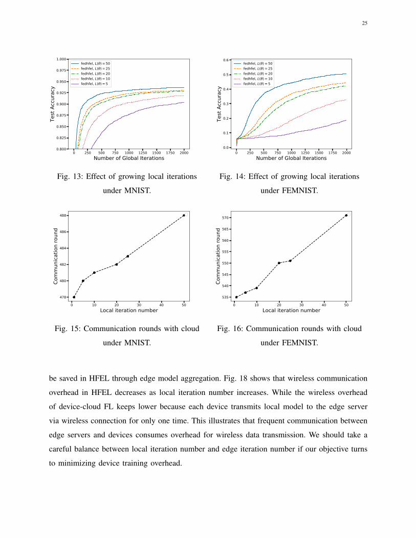
The effect of different local iteration numbers L(θ) = [5, 10, 20, 25, 50] on convergence speed

is exhibited in Fig. 13 and 14 through 2000 global iterations. As we can see, with the same

number of edge iterations as 5 and an increase of local iteration number from 5 to 50, the

convergence speed shows an obvious acceleration both in MNIST and FEMNIST datasets, which

implies the growth of L(θ) has a positive impact on convergence time.

Then we conduct experiments considering a fixed product of L(θ) and I(ε, θ) as 100 and the

values of L(θ) growing from 1 to 50. Fig. 15 and 16 show that a decreasing number of local

iterations and increasing number of edge iterations lead to a reduction of communication rounds

with the cloud to reach the accuracy of 0.9 for MNIST dataset and 0.55 for FEMNIST dataset,

respectively. Hence, properly increasing edge iteration rounds can help to reduce propagation

delay and improve convergence speed in HFEL.

Fig. 17 reveals a great advantage of WAN communication efficiency of HFEL over tradi-

tional device-cloud FL. Without edge aggregation, there are N devices’ local model parameters

transmitted through WAN to the remote cloud in device-cloud FL. While in HFEL, after edge

aggregation, K (generally K << N ) edge servers’ edge models, each of which is of similar size

to a local model, are transmitted to the cloud. Considerable WAN transmission overheads can

25

0 250 500 750 1000 1250 1500 1750 2000Number of Global Iterations

0.800

0.825

0.850

0.875

0.900

0.925

0.950

0.975

1.000Te

st A

ccur

acy

fedhfel, L( ) = 50fedhfel, L( ) = 25fedhfel, L( ) = 20fedhfel, L( ) = 10fedhfel, L( ) = 5

Fig. 13: Effect of growing local iterations

under MNIST.

0 250 500 750 1000 1250 1500 1750 2000Number of Global Iterations

0.0

0.1

0.2

0.3

0.4

0.5

0.6

Test

Acc

urac

y

fedhfel, L( ) = 50fedhfel, L( ) = 25fedhfel, L( ) = 20fedhfel, L( ) = 10fedhfel, L( ) = 5

Fig. 14: Effect of growing local iterations

under FEMNIST.

0 10 20 30 40 50Local iteration number

478

480

482

484

486

488

Com

mun

icatio

n ro

und

Fig. 15: Communication rounds with cloud

under MNIST.

0 10 20 30 40 50Local iteration number

535

540

545

550

555

560

565

570Co

mm

unica

tion

roun

d

Fig. 16: Communication rounds with cloud

under FEMNIST.

be saved in HFEL through edge model aggregation. Fig. 18 shows that wireless communication

overhead in HFEL decreases as local iteration number increases. While the wireless overhead

of device-cloud FL keeps lower because each device transmits local model to the edge server

via wireless connection for only one time. This illustrates that frequent communication between

edge servers and devices consumes overhead for wireless data transmission. We should take a

careful balance between local iteration number and edge iteration number if our objective turns

to minimizing device training overhead.

26

5 10 20 25 50Local iteration number

0.00

0.01

0.02

0.03

0.04

0.05W

AN d

elay

(s)

Device_cloud WAN delayHFEL WAN delay

Fig. 17: WAN communication overhead.

5 10 20 25 50Local iteration number

0

1

2

3

4

5

6

7

8

9

Wire

less

com

mun

icatio

n ov

erhe

ad Device_cloud wireless overheadHFEL wireless overhead

Fig. 18: Wireless communication overhead.

VI. RELATED WORK

To date, federated learning (FL) has been envisioned as a promising approach to guarantee

personal data security compared to conventional centralized training at the cloud. It only requires

local models trained by mobile devices with local datasets to be aggregated by the cloud such

that the global model can be updated iteratively until the training process converges.

Nevertheless, faced with long propagation delay in wide-area network (WAN), FL suffers

from a bottleneck of communication overhead due to thousands of communication rounds

required between mobile devices and the cloud. Hence a majority of studies have focused on

reducing communication cost in FL [23]–[26]. Authors in [23] proposed structured and sketched

local updates to reduce the model size transmitted from mobile devices to the cloud. While

authors in [24] introduced lossy compression and federated dropout to reduce cloud-to-device

communication cost, extending the work in [23]. [25] figured out a communication-mitigated

federated learning (CMFL) algorithm in which devices only upload local updates with high

relevance scores to the cloud. Further, considering that communication overhead often dominates

computation overhead [8], authors in [26] increased computation on each device during a local

training round by modifying the classic federated averaging algorithm in [8] as LoAdaBoost

FedAvg. While in our work, thanks to the emergence of mobile edge computing (MEC) which

migrates computing tasks from the network core to the network edge, we propose a hierarchical

Federated Edge Learning (HFEL) framework. In HFEL, mobile devices first upload local models

to proximate edge servers for partial model aggregation which can offer faster response rate and

27

relieve core network congestion.

Similarly, some existing literature also proposed hierarchical federated learning in MEC such

as [27] which presented a faster convergence speed than the FedAvg algorithm. Although a

basic architecture about hierarchical federated learning has been built in [27], the heterogeneity

of mobile device involved in FL is not considered. When large-scale devices with different

dataset qualities, computation capacities and battery states participate in FL, resource allocation

needs to be optimized to achieve cost efficient training.

There have been several existing research on the resource allocation optimization of mobile de-

vices for different efficiency maximization objectives in edge-assisted FL [15], [17], [28]–[32]. Yu

et al. worked on federated learning based proactive content caching (FPCC) [28]. While Nishio

et al. proposed an FL protocal called FedCS to maximize the participating number of devices

with a predefined deadline based on their wireless channel states and computing capacities [29].

Further, the authors extended their study of FedCS to [30] in which data distribution differences

are considered and solved by constructing independent identically distributed (IID) dataset. In

[31], the authors aimed at accelerating training process via optimizing batchsize selection and

communication resource allocation in a federated edge learning (FEEL) framework. [32] explored

energy-efficient radio resource management in FL and proposed energy-efficient strategies for

bandwidth allocation and edge association. Dinh et al. worked on a resource allocation problem

that captures the trade-off between convergence time and energy cost in FL [15]. While in

[17], local accuracy, transmit power, data rate and devices’ computing capacities were jointly

optimized for FL training time minimization.

In our HFEL framework, we target at solving computation and bandwidth resource allocation

of each device for training cost minimization in terms of energy and delay. Furthermore, edge

association is optimized for each edge server under the scenario where more than one edge

server is involved in HFEL and each device is able to communicate with multiple edge servers.

While the literature [15], [17], [31], [32] take only one edge server into account for resource

allocation. Along a different line, we work on training cost minimization in terms of energy and

delay by considering 1) joint computation and bandwidth resource allocation for each device

and 2) edge association for each edge server.

28

VII. CONCLUSION

Federated Learning (FL) has been proposed as an appealing approach to handle data security

issue of mobile devices compared to conventional machine learning at the remote cloud with raw

data. To enable great potentials in low-latency and energy-efficient FL, we introduce hierarchical

Federated Edge Learning (HFEL) framework in which model aggregation is partially migrated

to edge servers from the cloud. Furthermore, a joint computation and communication resource

scheduling model under HFEL framework is formulated to achieve global cost minimization.

Yet proving the minimization problem owns extremely high time complexity, we devise an

efficient resource scheduling algorithm which can be decomposed into two subproblems: resource

allocation given a scheduled set of devices for each edge server and edge association for all the

edge servers. Through cost reducing iterations of solving resource allocation and edge association,

our proposed HFEL algorithm terminates to a stable system point where it fulfills substantial

performance gain in cost reduction compared with the benchmarks.

Eventually, compared to conventional federated learning without edge servers as intermediaries

[8], the HFEL framework accomplishes higher global and test accuracies and lower training loss

as our simulation results show.

REFERENCES

[1] Z. Zhou, X. Chen, E. Li, L. Zeng, K. Luo, and J. Zhang, “Edge intelligence: Paving the last mile of artificial intelligence

with edge computing,” Proceedings of the IEEE, vol. 107, no. 8, pp. 1738–1762, Aug 2019.

[2] I. Goodfellow, Y. Bengio, and A. Courville, Deep learning. MIT press, 2016, http://www.deeplearningbook.org.

[3] P. Li, J. Li, Z. Huang, T. Li, C.-Z. Gao, S.-M. Yiu, and K. Chen, “Multi-key privacy-preserving deep learning in cloud

computing,” Future Generation Computer Systems, vol. 74, pp. 76 – 85, 2017.

[4] B. Custers, A. M. Sears, F. Dechesne, I. Georgieva, T. Tani, and S. van der Hof, EU Personal Data Protection in Policy

and Practice. Springer, 2019.

[5] B. M. Gaff, H. E. Sussman, and J. Geetter, “Privacy and big data,” Computer, vol. 47, no. 6, pp. 7–9, June 2014.

[6] A. Anonymous, “Consumer data privacy in a networked world: A framework for protecting privacy and promoting

innovation in the global digital economy,” Journal of Privacy and Confidentiality, vol. 4, no. 2, Mar. 2013. [Online].

Available: https://journalprivacyconfidentiality.org/index.php/jpc/article/view/623

[7] J. Konecny, H. B. McMahan, D. Ramage, and P. Richtárik, “Federated optimization: Distributed machine learning for

on-device intelligence,” arXiv preprint arXiv:1610.02527, 2016.

[8] H. Brendan McMahan, E. Moore, D. Ramage, S. Hampson, and B. Agüera y Arcas, “Communication-Efficient Learning

of Deep Networks from Decentralized Data,” Artificial Intelligence and Statistics, pp. 1273–1282, Apr 2017.

[9] M. Sviridenko, “A note on maximizing a submodular set function subject to a knapsack constraint,” Operations Research

Letters, vol. 32, no. 1, pp. 41–43, 2004.

29

[10] W. Shi, J. Cao, Q. Zhang, Y. Li, and L. Xu, “Edge computing: Vision and challenges,” IEEE Internet of Things Journal,

vol. 3, no. 5, pp. 637–646, Oct 2016.

[11] X. Chen, L. Jiao, W. Li, and X. Fu, “Efficient multi-user computation offloading for mobile-edge cloud computing,”

IEEE/ACM Transactions on Networking, vol. 24, no. 5, pp. 2795–2808, 2015.

[12] E. Li, L. Zeng, Z. Zhou, and X. Chen, “Edge ai: On-demand accelerating deep neural network inference via edge

computing,” IEEE Transactions on Wireless Communications, vol. 19, no. 1, pp. 447–457, Jan 2020.

[13] C. You, K. Huang, H. Chae, and B. Kim, “Energy-efficient resource allocation for mobile-edge computation offloading,”

IEEE Transactions on Wireless Communications, vol. 16, no. 3, pp. 1397–1411, March 2017.

[14] J. Konecny, Z. Qu, and P. Richtárik, “Semi-stochastic coordinate descent,” Optimization Methods and Software, vol. 32,

no. 5, pp. 993–1005, 2017.

[15] C. Dinh, N. H. Tran, M. N. Nguyen, C. S. Hong, W. Bao, A. Zomaya, and V. Gramoli, “Federated learning over wireless

networks: Convergence analysis and resource allocation,” arXiv preprint arXiv:1910.13067, 2019.

[16] T. D. Burd and R. W. Brodersen, “Processor design for portable systems,” Journal of Vlsi Signal Processing Systems for

Signal Image & Video Technology, vol. 13, no. 2-3, pp. 203–221, 1996.

[17] T. T. Vu, D. T. Ngo, N. H. Tran, H. Q. Ngo, M. N. Dao, and R. H. Middleton, “Cell-free massive mimo for wireless

federated learning,” arXiv preprint arXiv:1909.12567, 2019.

[18] C. Ma, J. Konecny, M. Jaggi, V. Smith, M. I. Jordan, P. Richtárik, and M. Takác, “Distributed optimization with arbitrary

local solvers,” Optimization Methods and Software, vol. 32, no. 4, pp. 813–848, 2017.

[19] “Stirling number of the second kind,” http://mathworld.wolfram.com/StirlingNumberoftheSecondKind.html.

[20] Y. Lecun, L. Bottou, Y. Bengio, and P. Haffner, “Gradient-based learning applied to document recognition,” Proceedings

of the IEEE, vol. 86, pp. 2278 – 2324, 12 1998.

[21] T. Li, A. K. Sahu, M. Zaheer, M. Sanjabi, A. Talwalkar, and V. Smith, “Federated optimization in heterogeneous networks,”

arXiv preprint arXiv:1812.06127, 2018.

[22] S. Caldas, P. Wu, T. Li, J. Konecny, H. B. McMahan, V. Smith, and A. Talwalkar, “Leaf: A benchmark for federated

settings,” arXiv preprint arXiv:1812.01097, 2018.

[23] J. Konecny, H. B. McMahan, F. X. Yu, P. Richtárik, A. T. Suresh, and D. Bacon, “Federated learning: Strategies for

improving communication efficiency,” arXiv preprint arXiv:1610.05492, 2016.

[24] S. Caldas, J. Konecny, H. B. McMahan, and A. Talwalkar, “Expanding the reach of federated learning by reducing client

resource requirements,” arXiv preprint arXiv:1812.07210, 2018.

[25] L. WANG, W. WANG, and B. LI, “Cmfl: Mitigating communication overhead for federated learning,” in 2019 IEEE 39th

International Conference on Distributed Computing Systems (ICDCS), July 2019, pp. 954–964.

[26] L. Huang, Y. Yin, Z. Fu, S. Zhang, H. Deng, and D. Liu, “Loadaboost: Loss-based adaboost federated machine learning

on medical data,” arXiv preprint arXiv:1811.12629, 2018.

[27] L. Liu, J. Zhang, S. Song, and K. B. Letaief, “Edge-assisted hierarchical federated learning with non-iid data,” arXiv

preprint arXiv:1905.06641, 2019.

[28] Z. Yu, J. Hu, G. Min, H. Lu, Z. Zhao, H. Wang, and N. Georgalas, “Federated learning based proactive content caching

in edge computing,” in 2018 IEEE Global Communications Conference (GLOBECOM), Dec 2018, pp. 1–6.

[29] T. Nishio and R. Yonetani, “Client selection for federated learning with heterogeneous resources in mobile edge,” in ICC

2019 - 2019 IEEE International Conference on Communications (ICC), May 2019, pp. 1–7.

[30] N. Yoshida, T. Nishio, M. Morikura, K. Yamamoto, and R. Yonetani, “Hybrid-fl for wireless networks: Cooperative learning

mechanism using non-iid data,” arXiv preprint arXiv:1905.07210, 2019.

30

[31] J. Ren, G. Yu, and G. Ding, “Accelerating dnn training in wireless federated edge learning system,” arXiv preprint

arXiv:1905.09712, 2019.

[32] Q. Zeng, Y. Du, K. K. Leung, and K. Huang, “Energy-efficient radio resource allocation for federated edge learning,”

arXiv preprint arXiv:1907.06040, 2019.