Heteroskedasticity Autocorrelation Robust Inference in

Time Series Regressions with Missing Data

Seung-Hwa Rho Timothy J. Vogelsang*

Louisiana State University† Michigan State University‡

May 19, 2017

Abstract

In this paper we investigate the properties of heteroskedasticity and autocorrelation robust (HAR)test statistics in time series regression settings when observations are missing. We primarily focus onthe non-random missing process case where we treat the missing locations to be fixed as T → ∞ bymapping the missing and observed cutoff dates into points on [0, 1] based on the proportion of timeperiods in the sample that occur up to those cutoff dates. We consider two models, the amplitudemodulated series (Parzen (1963)) regression model, which amounts to plugging in zeros for missingobservations, and the equal space regression model, which simply ignores the missing observations.When the amplitude modulated series regression model is used, the fixed-b limits of the HAR teststatistics depend on the locations of missing observations but are otherwise pivotal. When the equalspace regression model is used, the fixed-b limits of the HAR test statistics have the standard fixed-blimits as in Kiefer and Vogelsang (2005). We discuss methods for obtaining fixed-b critical values witha focus on bootstrap methods and find the naive i.i.d. bootstrap with missing dates fixed to be aneffective and practical way to obtain the fixed-b critical values.

Keywords: Missing data; Unequally spaced; Irregularly observed; Serial correlation robust

*We are grateful for helpful suggestions and comments from the anonymous referees and seminar participants at ColumbiaUniversity and the Joint Montreal Econometrics Seminar.

†Department of Economics, srho@lsu.edu‡Department of Economics, tvj@msu.edu

1

1 INTRODUCTION

It is not unusual to encounter a time series data set with missing observations but in a relatively simple

context of time series regression, there appears to be a sparsity of work related to missing data issues.

Most of the times series literature on missing data focuses on the estimation of dynamic models where

the goal is to forecast missing observations and little appears to be known about the impact of missing

data on heteroskedasticity and autocorrelation robust (HAR) tests in regression settings. This paper

attempts to fill this void by analyzing the impact of missing data on HAR tests based on nonparametric

kernel estimators of long run variances (HAR variance estimators).

We consider the case where the missing process is exogenous to the underlying latent process and

the estimators are identified by the observed data. Hence we are not proposing a new estimator. Our

focus rather lies on the impact of missing data on the long run variance estimator and further deriving

a reference distribution for HAR inference which captures the impact of missing observations. We con-

sider two models, the amplitude modulated (AM) series and equal space (ES) regression models. The

ES regression model, which is formally considered in Datta and Du (2012), simply ignores the missing

observations and treats the observations as if they are equally spaced in time. The AM regression model,

first proposed by Parzen (1963), characterizes the missing observations as being driven by a 0-1 binary

missing process. In terms of a regression model this amounts to plugging in zeros for missing observa-

tions. The literature following Parzen (1963) mainly focused on investigating the impact of missing data

on the consistent estimation of spectral density functions of the underlying latent series. See, for exam-

ple, Scheinok (1965), Bloomfield (1970), Neave (1970), and Dunsmuir and Robinson (1981).1 While HAR

inference makes use of spectral estimation methods, with the exception of Datta and Du (2012), there

appears to be no attempt in the literature to link this earlier literature on spectral density estimation to

regression inference with missing data.

The AM approach appears to be intuitively more sensible than the ES approach because the time dis-

tances between observations become skewed for many pairs of time periods for the ES approach while

the time distances are preserved for the AM approach. This would seem particularly relevant for testing

based on HAR variance estimators (e.g.,Newey and West (1987), Andrews (1991)) given that those esti-

1Scheinok (1965) and Bloomfield (1970) consider estimating a spectral density function of the observed process (withmissing data) with independent Bernoulli and dependent Bernoulli missing processes respectively. Neave (1970) estimatesa spectral density function with initially scarce data. Later work by Dunsmuir and Robinson (1981) investigated consistentestimation of the spectral density of the underlying latent process.

2

mators employ quadratic forms with weights that depend on the time distances of pairs of observations.

One might reasonably conjecture (and we also conjectured) that the ES approach would be problem-

atic. In practice the AM approach is prominent, but the ES approach is still used. For example, in the

statistical package Stata, the command newey with the ’force’ option computes Newey-West standard

errors using the AM approach whereas the command newey2 with the ’force’ option or the command

hacreg computes Newey-West standard errors based on the ES approach. Surprisingly, we find that the

ES approach can be justified theoretically with the fixed-b asymptotic framework and works better than

one might expect.

Our work is most closely related to Datta and Du (2012) who also analyze the AM and ES approaches

in time series regressions with missing data. Their results provide a good foundation for the traditional

small bandwidth asymptotic theory on HAR tests which appeals to consistency of the HAR variance es-

timators. Our results, on the other hand, are based on fixed-b asymptotic framework as in Kiefer and

Vogelsang (2005). The fixed-b results that we obtain can be viewed as useful refinements to the tradi-

tional theory because it is now well established that fixed-b theory provides improved approximations

by capturing much of the impact of kernel and bandwidth choices on finite sample distributions of HAR

tests (see e.g., Jansson (2002), Sun et al. (2008), Goncalves and Vogelsang (2011)). In addition, we show

that it is possible to capture the impact of missing data on HAR robust tests via the asymptotic reference

distribution. This is done by mapping the missing locations into points on [0, 1] as fixed proportions of

the total time span. This mapping is conceptually the same as mapping a given number of break dates

to corresponding break points in a model with structural change and obtaining asymptotic results hold-

ing the break points fixed as T → ∞. Having critical values that depend on the missing dates improves

the reliability of finite sample inference.

The following are the main theoretical findings in the paper. (1) When the missing process is non-

random, the fixed-b limits of the HAR Wald statistics computed from the AM approach depend on the

locations of missing observations in addition to the kernel function and the bandwidth used but are

otherwise pivotal. (2) When the missing data are simply ignored (ES approach), we find that the fixed-b

limits of the HAR Wald statistics are the standard fixed-b distribution as in Kiefer and Vogelsang (2005).

(3) We also investigate methods for obtaining fixed-b critical values with a focus on bootstrap methods.

We show that the results of Goncalves and Vogelsang (2011) extend to both the AM and ES approaches.

The naive i.i.d. bootstrap is a particularly good option for obtaining valid fixed-b critical values especially

if the dates of the missing observations are taken as given when generating bootstrap samples.

3

It is important to draw similarities and differences between the results in this paper and recent work

by Bester et al. (2016) who obtained fixed-b results in spatial settings. In spatial settings the sample

region can have varied shapes and the shape can affect the sampling distribution of HAR tests. Bester

et al. (2016) show that the shape of the sampling region is captured by fixed-b theory. This is similar

to our result where the fixed-b limit depends on the dates (locations) of missing data when the missing

process is non-random. One might wonder whether the results of Bester et al. (2016) can be directly

applied to missing data in time series settings because Bester et al. (2016) obtain results using random

field theory and a time series process is a one-dimensional random field. The answer is no because

Bester et al. (2016) restrict attention to two-dimensional sampling regions with quadrant-wise mono-

tonic boundaries which rules out holes in the sampling region. Missing observations generate holes in

the sampling region and therefore the results in Bester et al. (2016) do not directly apply.

The rest of the paper is organized as follows. Section 2 defines the models, estimators, and relevant

test statistics. Section 3 develops fixed-b asymptotic results for the estimators and the test statistics

defined in Section 2. Section 4 discusses simulation of the asymptotic critical values with a focus on

bootstrap methods. Finite sample performance is examined in Section 5 by Monte Carlo simulations.

Attention is focused on the relative performance of simulated asymptotic critical values compared with

bootstrap critical values and the relative performance of the AM approach compared with the ES ap-

proach. Practical recommendations are given. Section 6 concludes. Formal proofs for the fixed-b results

are given in Appendices A-B for the AM and ES approaches respectively.

2 MODELS AND TEST STATISTICS

2.1 Models

Suppose that a researcher is interested in the regression model

y∗t = x∗′

t β + u∗t , (t = 1, 2, . . . , T) , (1)

where y∗t (scalar) and x∗t (k× 1 vector) are latent variables that are not fully observed in the missing data

case. Suppose that the k× 1 vector of parameters, β, is identified by the moment condition

E(m (w∗t ; β)) = 0, (2)

4

where w∗′t = (y∗t , x∗′

t ) and

m (w∗t ; β) = x∗t (y∗t − x∗

′t β) = x∗t u∗t .

Let at be a missing process where

at =

1 when all g elements in w∗t are observed at time t

0 otherwise.

If we assume that the mechanism generating the missing data does not generate an endogeneity prob-

lem, then the moment condition (2) above implies

E(atm (w∗t ; β)) = E(

atx∗t (y∗t − x∗

′t β)

)= E (atx∗t u∗t ) = 0, (3)

which puts zero weight on time period t whenever at least one element of w∗t is not observed.2 We

maintain assumption (3) throughout the paper so that we can focus on the impact of missing data on

HAR inference in settings where β is identified by the observed data.

We consider two regression models, the AM and ES regression models, which are naturally related to

(3). The AM regression model, proposed by Parzen (1963),3 is given by

yt = x′tβ + ut, (t = 1, 2, . . . , T) , (4)

where yt = aty∗t , xt = atx∗t , and ut = atu∗t . The ordinary least squares (OLS) moment condition,

E(xt(yt − x′tβ)) = 0, is easily seen to be the same as (3) using the fact that a2t = at. Practically speaking,

zeros are plugged in for y∗t and x∗t for any time period that has a missing observation in y∗t and/or any

element of x∗t . Because the zeros act as place holders for missing observations, the true time distances

between observations are preserved. At a conceptual level this would appear important when using

HAR variance estimators to obtain robust standard errors.

The ES regression model is obtained by ignoring time periods with missing data and re-indexing the

2As pointed out by the referees, applying the missing process to the moment condition rather than the regression modelitself allows xt to contain lags of yt. However, we do not explicitly consider dynamic models in this paper because eitherdynamic completeness holds in which case the HAR variance estimator would not be required or dynamic completeness failsin which case (3) does not hold and β is not identified.

3Parzen (1963) adopted the label, amplitude modulated series, because the original time series are amplitude modulatedby the missing process at.

5

observed time periods.4 The observed time series processes for the ES regression model are yESτ =

y∗t , xESτ = x∗t ; τ = ∑t

s=1 asTESτ=1, where TES = ∑T

t=1 at is the number of time periods with no missing data

(see Figure 1 below). This leads to the ES regression model

yESτ = xES′

τ β + uESτ , (τ = 1, 2, . . . , TES) . (5)

Similar to the AM regression model, the OLS moment condition for (5) is equivalent to (3) with the

missing time periods ignored and observed time periods reindexed. Because the ES approach changes

the time index, time distances between observations become skewed for many pairs of time periods

when computing an HAR variance estimator. For example, in Figure 1, wES5 and wES

6 , which are 5 time

periods apart, are treated as if they are a single time period away.

data←−−−−−−−−−−−→v v v v v f f f f v v v fwES

1

missing←−−−−−−−−→

wES5

data←−−−−→

wES6 = w∗10 6 = ∑10

t=1 at

. . .data←−−−−−−−→f v v v v

wESTES−3 wES

TES

Figure 1: Equal Space Regression Model

In fact, in terms of estimating β, there is no difference between the AM and ES regression models. Let

β be obtained by the sample analog to (3):

1T

T

∑t=1

atx∗t (y∗t − x∗

′t β) = 0.

Because ∑ atx∗t (y∗t − x∗

′t β) = 0 can be equivalently written as

T

∑t=1

atx∗t (y∗t − x∗

′t β) =

T

∑t=1

xt(yt − x′t β) =TES

∑τ=1

xESτ (yES

τ − xES′τ β) = 0,

it follows that β is the OLS estimator in both the AM and ES regression models.5

4The label ‘equal space’ was adopted by Datta and Du (2012) because the observations in the ES regression are adjacent toeach other after reindexing time.

5The equivalence between the AM and ES approaches for parameter estimation could extend to models with more generalmoment conditions that are exactly identified. However, in the case of over-identified models, this equivalence will not holdin general. For example it will break down if the weighting matrix used for generalized method of moments (GMM) estimatoris based on a nonparametric kernel covariance matrix estimator because the reindexing of time in the ES approach wouldmake the covariance matrix estimators in the AM and ES approaches different. Using the fixed smoothing theory for GMMdeveloped by Sun (2014a), it should be possible to extend the results we obtain here to a more general GMM setting, but suchan extension is nontrivial and is beyond the current scope of this paper.

6

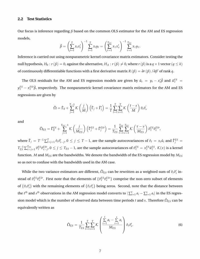
2.2 Test Statistics

Our focus is inference regarding β based on the common OLS estimator for the AM and ES regression

models,

β =

(T

∑t=1

xtx′t

)−1 T

∑t=1

xtyt =

(TES

∑τ=1

xτx′τ

)−1 TES

∑τ=1

xτyτ.

Inference is carried out using nonparametric kernel covariance matrix estimators. Consider testing the

null hypothesis, H0 : r (β) = 0, against the alternative, HA : r (β) 6= 0, where r (β) is a q× 1 vector (q ≤ k)

of continuously differentiable functions with a first derivative matrix R (β) = ∂r (β) /∂β′ of rank q.

The OLS residuals for the AM and ES regression models are given by ut = yt − x′t β and uESτ =

yESτ − xES′

τ β, respectively. The nonparametric kernel covariance matrix estimators for the AM and ES

regressions are given by

Ω = Γ0 +T−1

∑j=1K(

jM

)(Γj + Γ′j

)=

1T

T

∑t=1

T

∑s=1K(

t− sM

)vtv

′s

and

ΩES = ΓES0 +

TES−1

∑j=1K(

jMES

)(ΓES

j + ΓES′j

)=

1TES

TES

∑τ=1

TES

∑ν=1K(

τ − ν

MES

)vES

τ vES′ν ,

where Γj = T−1 ∑Tt=j+1 vtv′t−j, 0 ≤ j ≤ T − 1, are the sample autocovariances of vt = xtut and ΓES

j =

T−1ES ∑TES

τ=j+1 vESτ vES′

τ−j, 0 ≤ j ≤ TES − 1, are the sample autocovariances of vESτ = xES

τ uESτ . K(x) is a kernel

function. M and MES are the bandwidths. We denote the bandwidth of the ES regression model by MES

so as not to confuse with the bandwidth used in the AM case.

While the two variance estimators are different, ΩES can be rewritten as a weighted sum of vtv′s in-

stead of vESτ vES′

ν . First note that the elements of vESτ vES′

ν comprise the non-zero subset of elements

of vtv′s with the remaining elements of vtv′s being zeros. Second, note that the distance between

the tth and sth observations in the AM regression model converts to |∑ti=1 ai − ∑s

i=1 ai| in the ES regres-

sion model which is the number of observed data between time periods t and s. Therefore ΩES can be

equivalently written as

ΩES =1

TES

T

∑t=1

T

∑s=1K

t

∑i=1

ai −s∑

i=1ai

MES

vtv′s. (6)

7

Using the OLS estimator and the robust variance estimators, the HAR Wald statistics are defined as

WT = Tr(

β)′ [

R(

β)

Q−1ΩQ−1R(

β)′]−1

r(

β)

and (7)

WEST = TESr

(β)′ [

R(

β)

Q−1ES ΩESQ−1

ES R(

β)′]−1

r(

β)

for the AM and ES regressions respectively, where Q = T−1 ∑Tt=1 xtx′t and QES = T−1

ES ∑TESτ=1 xES

τ xES′τ . For

the single restriction (q = 1) case, the corresponding t-statistics are

tT =

√Tr(

β)√

R(

β)

Q−1ΩQ−1R(

β)′ and tES

T =

√TESr

(β)√

R(

β)

Q−1ES ΩESQ−1

ES R(

β)′ . (8)

To better compare WEST with WT, rewrite WES

T using QES = (T/TES) Q as

WEST = Tr

(β)′ [

R(

β)

Q−1(

TES

TΩES

)Q−1R

(β)′]−1

r(

β)

. (9)

It immediately follows that WEST in (9) has the exact same form as WT in (7) with (TES/T) ΩES used in place

of Ω. Furthermore, using (6), WEST becomes

WEST = Tr

(β)′ [

R(

β)

Q−1ΩKQ−1R(

β)′]−1

r(

β)

,

where ΩK ≡1T

T

∑t=1

T

∑s=1K

t

∑i=1

ai −s∑

i=1ai

MES

vtv′s.

Hence, in terms of the test statistics, choosing between the AM approach and the ES approach boils

down to a choice of kernel function betweenK ((t− s)/M) and K(t, s, MES) ≡ K ((∑ti=1 ai −∑s

i=1 ai)/MES) when

computing the HAR variance estimator. Suppose the same kernel and bandwidth are used for the AM

and ES approaches with M = MES. Then

∣∣∣∣ t∑

i=1ai −

s∑

i=1ai

∣∣∣∣MES

≤ |t− s|M

,

in which case it follows that less down-weighting on vtv′s is used in the ES approach because the ES

regression model ignores the gaps created by the missing observations. The bottom line is that, for a

given kernel and bandwidth, the ES Wald statistic has an equivalent AM Wald statistic where the HAR

variance estimator is based on a weighting scheme that is a transformed version of the ES weighting

8

scheme.

3 ASSUMPTIONS AND ASYMPTOTIC THEORY

In this section, we derive the asymptotic behavior of the OLS estimator, the HAR variance estimators,

and the Wald statistics defined in Section 2. Our primary focus is on obtaining fixed-b asymptotic re-

sults. Throughout, the symbol “⇒” denotes weak convergence of a sequence of stochastic processes to

a limiting stochastic process andWq(r) denotes a q× 1 vector of independent standard Wiener process.

Following Sun (2014b) we make the following assumption on the kernel function.

AssumptionK. The kernel functionK(x) : R→ [0, 1] is symmetric, piecewise smooth withK(0) = 1 and∫ ∞0 K(x)xdx < ∞.

AssumptionK imposes mild conditions on the kernel function and most of the kernel functions used

in practice - including Bartlett, Parzen, and QS kernels - satisfy this assumption. With Assumption K,

Kb(r, s) ≡ Kb(r− s) = K((r− s)/b) defined on [0, 1]× [0, 1] for every given b is symmetric and integrable

in L2([0, 1]× [0, 1]) and we can expand Kb(r, s) as Kb(r, s) = ∑∞n=1 νn fn(r) fn(s). Here νn is an eigenvalue

of the kernel and fn(s) is the corresponding eigenfunction so that νn fn(s) =∫ 1

0 Kb(r, s) fn(r)dr. See Sun

(2014b) for details.

3.1 Random Missing Process

In this section, we briefly discuss the random missing process case. We only sketch some results given

that our main interest is the non-random missing process case. Suppose at is a random process

such that (3) holds. A sufficient condition for (3) is that at is independent from the latent processes

(u∗t , x∗′t )′. The weaker condition such as E(u∗t |at, x∗t ) = 0 with E(u∗t |x∗t ) = 0 is also sufficient.

When the missing process is random, the asymptotic theory is driven by the observed AM series.

Suppose the observed AM series satisfies the following for r ∈ [0, 1]: (a) T−1 ∑[rT]t=1 xtx′t ⇒ rQ, uniformly

in r with Q full rank, and (b) T−1/2 ∑[rT]t=1 vt ⇒ ΛWk (r) where Λ is the matrix square root of the long run

variance matrix of vt. Then the HAR variance estimator and Wald statistics of the AM series have the

usual fixed-b asymptotic limits as obtained by Kiefer and Vogelsang (2005). These conditions would be

9

satisfied if the latent and missing processes are jointly weakly dependent with proper moment condi-

tions. A set of primitive conditions on missing and latent processes that are sufficient for these high

level assumptions are lengthy but standard. Interested readers can refer the Supplemental Appendix

available on our website.6

For the ES approach, suppose the ES regression model satisfies the following for r ∈ [0, 1]: (a) T−1ES ∑[rTES]

τ=1 xτx′τ ⇒

rQES, uniformly in r with QES full rank, and (b) T−1/2ES ∑[rTES]

τ=1 vESτ ⇒ ΛESWk(r) where ΛES is the matrix

square root of the long run variance matrix of vESτ . Then the HAR variance estimator and Wald test

statistics of the ES regression model have the usual fixed-b asymptotic limits as in Kiefer and Vogelsang

(2005). Because the ES processes have less dependence than the latent processes, it is reasonable to

conjecture that ES processes will satisfy conditions (a) and (b) above whenever the latent processes sat-

isfies conditions analogous to (a) and (b). This is trivially true when the latent processes are white noise

processes. In other words, if the latent processes satisfy conditions required for fixed-b theory then the

asymptotic fixed-b distribution for the ES approach would be identical to the usual fixed-b distribution.

Hence, from a fixed-b perspective, the random missing process case is rather trivial when the miss-

ing processes are weakly dependent and satisfy the key assumptions for obtaining a fixed-b limit. The

theory is more interesting when at is viewed as a non-random process.

3.2 Non-random missing process

In this section, we analyze the asymptotic behavior of the OLS estimator and the HAR test statistics de-

fined in Section 2 under the assumption that the missing process is non-random. The theory developed

in this section is used to obtain an asymptotic reference distribution for the HAR test statistics that de-

pends on the locations of the missing data in a given sample. We begin by describing the timing of the

missing observations for an arbitrary data set.

Definition 1. [Timing of the missing observations] We characterize an arbitrary data set with missing

observations as follows. From t = 1 to t = T1 we observe data, from t = T1 + 1 to t = T2 data are missing,

from t = T2 + 1 to t = T3 we observe data and so forth. Let the number of missing clusters be C. For

simplicity, we assume that data are observed at t = 1 and t = T.7 Thus, in general, from t = T2n−1 + 1 to

6http://msu.edu/∼ tjv/working.html7This assumption is only for notational simplicity. The results of this paper go through without this assumption.

10

t = T2n data are missing whereas from t = T2n + 1 to t = T2n+1 data are observed, n = 1, . . . , C (see Figure

2). For notational purposes, let T0 = 0 and T2C+1 = T.

data←−−−−−−−−−−−→v v v v v f f f f v v v f

t = 1

missing←−−−−−−−→

t = T1

data←−−−−→

t = T2 t = T3

. . .data

←−−−−−−−→f v v v vt = T2C t = T

Figure 2: Timing of the data with missing observations

When the missing process is non-random, missing locations are non-random, and hence the finite

sample behavior of the estimators and statistics will depend on the locations of missing observations.

To capture this dependence on missing locations in the asymptotic theory, we map the missing and

observed cutoff dates into points on [0, 1] based on the proportion of time periods in the sample that

occur up to a particular cutoff date, Ti, by defining λi = Ti/T for i = 0, 1, . . . , 2C + 1. By definition,

T0 = 0 and T2C+1 = T and it follows that λ0 = 0 and λ2C+1 = 1.

Once a researcher obtains the data, the number of missing clusters and the locations of the missing

observations are known. Since these locations are defined within the obtained sample with time span

T, they are fully characterized by the set of ratios λ1, . . . , λ2C which we denote as λi. In order to

obtain useful asymptotic results that capture the locations of the cutoff dates, we treat λi and C fixed

as T → ∞, which is stated below.

Assumption fixed-λ. Let the missing and observed cutoff dates be Ti and C be the number of missing

clusters as defined in Definition 1. When the missing process is non-random, we let

λi ≡Ti

T, i = 0, 1, . . . , 2C + 1,

and C < ∞ be fixed as T → ∞.

Intuitively, we are preserving the relative finite sample locations of the missing clusters when obtain-

ing our asymptotic results. It is important to keep in mind that this asymptotic nesting is only used to

obtain reference distributions for generating critical values for test statistics and is not meant to be a

description of the way the data is gathered or generated. Following the suggestion of a referee, we label

this asymptotic nesting the ‘fixed-λ device’.8

8Conceptually, the fixed-λ device is the same as mapping a given number of break dates to corresponding breakpoints in amodel with structural change and obtaining asymptotic results holding the breakpoints fixed as T → ∞.

11

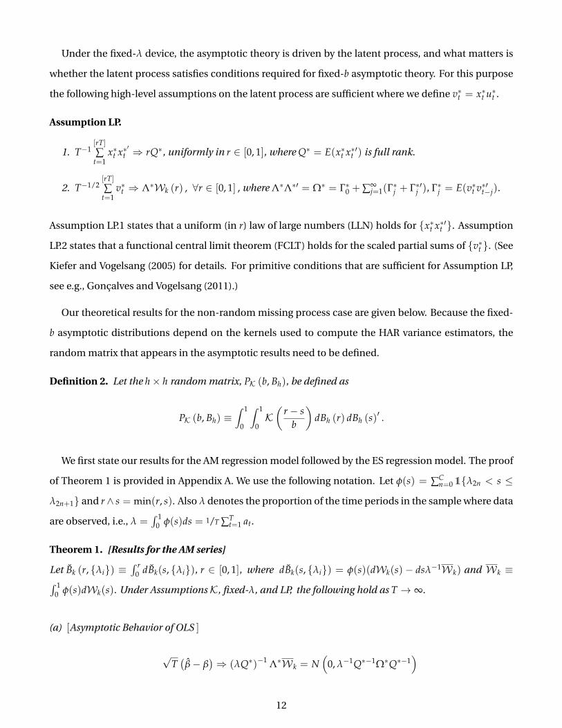
Under the fixed-λ device, the asymptotic theory is driven by the latent process, and what matters is

whether the latent process satisfies conditions required for fixed-b asymptotic theory. For this purpose

the following high-level assumptions on the latent process are sufficient where we define v∗t = x∗t u∗t .

Assumption LP.

1. T−1[rT]∑

t=1x∗t x∗

′t ⇒ rQ∗, uniformly in r ∈ [0, 1], where Q∗ = E(x∗t x∗′t ) is full rank.

2. T−1/2[rT]∑

t=1v∗t ⇒ Λ∗Wk (r) , ∀r ∈ [0, 1] , where Λ∗Λ∗′ = Ω∗ = Γ∗0 + ∑∞

j=1(Γ∗j + Γ∗′j ), Γ∗j = E(v∗t v∗′t−j).

Assumption LP.1 states that a uniform (in r) law of large numbers (LLN) holds for x∗t x∗′t . Assumption

LP.2 states that a functional central limit theorem (FCLT) holds for the scaled partial sums of v∗t . (See

Kiefer and Vogelsang (2005) for details. For primitive conditions that are sufficient for Assumption LP,

see e.g., Goncalves and Vogelsang (2011).)

Our theoretical results for the non-random missing process case are given below. Because the fixed-

b asymptotic distributions depend on the kernels used to compute the HAR variance estimators, the

random matrix that appears in the asymptotic results need to be defined.

Definition 2. Let the h× h random matrix, PK (b, Bh), be defined as

PK (b, Bh) ≡∫ 1

0

∫ 1

0K(

r− sb

)dBh (r) dBh (s)

′ .

We first state our results for the AM regression model followed by the ES regression model. The proof

of Theorem 1 is provided in Appendix A. We use the following notation. Let φ(s) = ∑Cn=0 1λ2n < s ≤

λ2n+1 and r∧ s = min(r, s). Also λ denotes the proportion of the time periods in the sample where data

are observed, i.e., λ =∫ 1

0 φ(s)ds = 1/T ∑Tt=1 at.

Theorem 1. [Results for the AM series]

Let Bk (r, λi) ≡∫ r

0 dBk(s, λi), r ∈ [0, 1], where dBk(s, λi) = φ(s)(dWk(s)− dsλ−1W k) and W k ≡∫ 10 φ(s)dWk(s). Under AssumptionsK, fixed-λ, and LP, the following hold as T → ∞.

(a) [Asymptotic Behavior of OLS ]

√T(

β− β)⇒ (λQ∗)−1 Λ∗W k = N

(0, λ−1Q∗−1Ω∗Q∗−1

)

12

(b) [Fixed-b asymptotic limit of the HAR variance estimator ] Assume M = bT where b ∈ (0, 1] is fixed.

Then,

Ω⇒ Λ∗PK(b, Bk (λi)

)Λ∗′,

where PK(·) is given by Definition 2.

(c) [Fixed-b asymptotic distribution of WT ] Under H0 and M = bT where b ∈ (0, 1] is fixed,

WT ⇒W′q[PK(b, Bq (λi)

)]−1W q,

and when q = 1,

tT ⇒W1√

PK(b, B1(λi)

) .

According to Theorem 1(a) the asymptotic variance of the OLS estimator depends on Ω∗, the long run

variance of the latent process, even though WT is constructed using the AM series long run variance

estimator Ω. This poses no problems for inference because the fixed-b limit of Ω is proportional to Ω∗

through Λ∗ and Λ∗′ and Ω∗ cancels from the limiting distributions of the test statistics. Theorem 1(b)

shows that the fixed-b limit of Ω depends on PK (·) which takes the same form as in the usual fixed-b

limits in models with no missing data (Kiefer and Vogelsang (2005)). This is not surprising since test

statistics based on the AM series preserve the true time distances between observations and the kernel

weights stay the same even if there are missing observations. The key difference between the fixed-b

limit of Ω in Theorem 1(b) compared to that without missing observations is the form of Bk(r, λi), the

asymptotic limit of the partial sum T−1/2 ∑[rT]t=1 vt. When there are missing observations, Bk (r, λi) de-

pends on the locations of the missing observations via the fixed-λ device and is not a Brownian bridge.9

Hence the critical values generated by the reference distributions given by Theorem 1(c) depend on the

locations of the missing data and are different from the standard fixed-b critical values.10

Next, we state our result for the ES regression model. The proof for Theorem 2 is given in Appendix B.

Theorem 2. [Results for the ES regression model]

Define the k × 1 stochastic process...W k(r) = λ−1/2

∫ (rλ+∑2nk=1(−1)kλk)

0 φ(u)dWk(u) for n ∈ 0, . . . , C such

9This is shown formally in Appendix A.10Similar to Kiefer and Vogelsang (2005), Bk (r, λi) is independent ofW k. See Appendix A.

13

that rλ + ∑2nk=1(−1)kλk ∈ (λ2n, λ2n+1] and let

...W k(r) =

...W k(r)− r

...W k(1), r ∈ [0, 1]. Under Assumptions

K, fixed-λ, and LP, the following hold as T → ∞.

(a) [Asymptotic Behavior of OLS ]

√TES

(β− β

)⇒ Q∗−1Λ∗

...W k(1) = N

(0, Q∗−1Ω∗Q∗−1

)

(b) [Fixed-b asymptotic limit of ΩES ] Let MES = bTES where b ∈ (0, 1] is fixed. Then,

ΩES ⇒ Λ∗PK(

b,...W k

)Λ∗′,

where PK(·) is defined via Definition 2.

(c) [Fixed-b asymptotic distribution of WEST ] Let MES = bTES where b ∈ (0, 1] is fixed. Under H0,

WEST ⇒

...W q(1)′

[PK(

b,...W q

)]−1 ...W q(1),

and when q = 1,

tEST ⇒

...W1(1)√

PK(

b,...W1

) .

The asymptotic result for the OLS estimator given by Theorem 2(a) is identical to the result in The-

orem 1(a) because the AM and ES regression models have the same OLS estimator. Here λ−1 is gone

because the normalizing factor is√

TES instead of√

T. What is not obvious is that the asymptotic distri-

butions in Theorem 2(b) and (c) are in fact equivalent to the standard fixed-b asymptotic distributions

as in Kiefer and Vogelsang (2005) with b = MES/TES. Thus, we obtain the surprising result that when the

missing process is non-random, the HAR Wald test of the ES regression model has the usual fixed-b limit

that does not depend on the missing locations. This result holds because it can be shown that...W k(r) is

a vector of standard Wiener process (see Appendix B).

We can provide some intuition as to why the HAR statistics have the usual fixed-b limits in the ES

regression even though the ES approach contaminates the timing of the dates where data is observed.

Suppose the latent processes are i.i.d.. When the missing dates are ignored and dropped, we are left

14

with a regression model with TES observations and no serial correlation in the data. Therefore, WEST , the

usual HAR Wald statistic computed with TES observations, has the usual fixed-b limit as in Kiefer and

Vogelsang (2005) with b = MES/TES. Because fixed-b limits of HAR statistics naturally extend from the

i.i.d. case to cases with dependence due to the proportionality of the numerator and denominator to

the long run variance, the results obtained in Theorem 2(b) and (c) are less surprising given that they

trivially hold in the i.i.d. case.

4 BOOTSTRAP CRITICAL VALUES

In Section 3, we showed that when the missing process is non-random and the AM regression is used,

the HAR Wald statistic has a fixed-b asymptotic distribution that depends on the missing locations

through λi (‘λ,fixed-b’ distribution henceforth). We also showed that when the ES regression model

is used, the HAR Wald test statistic has the usual fixed-b asymptotic distribution. Both the usual fixed-b

and ‘λ,fixed-b’ distributions are non-standard but it is relatively straightforward to obtain the critical

values by directly simulating from the asymptotic distributions because they are functions of Brown-

ian motions.11 A potentially more user-friendly method, especially for the ‘λ,fixed-b’ distribution, is to

obtain critical values using the bootstrap.

In the fixed-b literature, Goncalves and Vogelsang (2011) showed that the naive moving block boot-

strap has the same limiting distribution as the fixed-b asymptotic distribution under suitable regularity

conditions. Their result hinges on the idea that if the bootstrap samples satisfy the LLN and FCLT that

are required for fixed-b theory to go through with the probability measure induced by the bootstrap

resampling conditional on a realization of the original time series (denoted as p• henceforth), then be-

cause the fixed-b asymptotic distribution depends on the kernel function and b = M/T but is otherwise

pivotal, the bootstrap statistic will have the same limiting distribution as the original test statistic. The

regularity conditions are those such that bootstrap samples satisfy the LLN and FCLT in the bootstrap

world.

In the presence of missing observations, the HAR Wald statistics have fixed-b asymptotic distribu-

tions which depend on the kernel function, b, and, for the case of the ‘λ,fixed-b’ distribution, λi, but

11For the usual fixed-b distribution, Vogelsang (2012) has developed a numerical method for the easy computation of stan-dard fixed-b critical values and p-values for any significance level when the Bartlett kernel is used. Kiefer and Vogelsang (2005)provide critical value functions for popular significance levels for a set of kernels.

15

are otherwise pivotal. Hence it is expected that similar results as in Goncalves and Vogelsang (2011)

would go through if the bootstrap samples for the AM series and the ES regression models satisfy As-

sumptions fixed-λ and LP under the probability measure p•. Assumption fixed-λ treats the locations of

missing data as fixed within the sample, so we need a bootstrap resampling scheme that preserves the

missing locations. This means that the moving block bootstrap with block length greater than one is

not practical because blocks will shuffle the locations of the missing data upon resampling. Instead, the

i.i.d. bootstrap is appropriate where bootstrap samples are created by first resampling with replacement

from the observed data and creating a bootstrap sample with the same missing locations as the original

data.

Define ωt = (yt, x′t)′, t = 1, . . . , T, that collects the dependent and independent variables of the AM

series. Among those T observations define the subset of only the observed data, which we denote ωt =

(yt, x′t)′, t = 1, . . . , T, T = ∑T

t=1 at. Using block length l = 1, resample T observations with replacement

from ωt and obtain a bootstrap sample for the ES regression model, which we denote as ω•t = (y•t , x•′

t )′,

t = 1, . . . , T. Using ω•t , construct the bootstrap sample for the AM series denoted as ω•t = (y•t , x•′t )′,

t = 1, . . . , T, by filling in the observed locations with resampled data ω•t and the missing locations with

zeros. This way we construct an i.i.d. bootstrap sample with missing locations that match those in the

observed data. The naive bootstrap test statistic for the AM regression, W•T, is computed with ω•t as

W•T = T(r(β•)− r(β)

)′[R(β•)Q•−1Ω•Q•−1R(β•)′]−1 (r(β•)− r(β)

), (10)

and the naive bootstrap test statistic for the ES regression model, WES•T , is computed with ω•t as

WES•T = T

(r(β•)− r(β)

)′[R(β•)Q•−1

ES Ω•ESQ•−1ES R(β•)′]−1 (r(β•)− r(β)

), (11)

where β• is the OLS estimator from the regression of y•t on x•t , Q• = 1/T ∑Tt=1 x•t x•′t , Q•ES = 1/T ∑T

τ=1 x•τ x•′τ ,

Ω• = 1/T ∑Tt=1 ∑T

t=1K ((t− s)/M) v•t v•′s where v•t = x•t (y•t − x•′t β•), and Ω•ES = 1/T ∑T

τ=1 ∑Tν=1K((τ − ν)/MES)v•τv•′ν

where v•τ = x•τ(y•τ − x•′τ β•). Note that bootstrap statistics use the same formula as WT and WEST , which is

why this approach is called the naive bootstrap.

Because we resample from observed time periods only, this resampling can be thought of as resam-

pling from the latent process ω∗t ≡ (y∗t , x∗′t )′. We do not know the value of ω∗t when at = 0 and thus

we are resampling from T observations not the full number of time periods T. However, because the

resampling is based on i.i.d. draws, this bootstrap sample has essentially the same properties as an i.i.d.

16

bootstrap sample of the fully observed latent process. We could take another T − T independent draws

from ωt and fill in the missing locations of ω•t . Call this “filled-in” bootstrap sample ω∗•t . Then by con-

struction ω•t = atω∗•t where ω∗•t can be viewed as a bootstrap sample from the latent process given the

i.i.d. resampling. If the bootstrap sample, ω∗•t , satisfies

(a) T−1[rT]

∑t=1

x∗•t x∗•′tp•⇒ rQ∗• and

(b) T−1/2[rT]

∑t=1

v∗•tp•⇒ Λ∗•Wk(r) (12)

for some Q∗• and Λ∗•, Assumption LP is satisfied for the bootstrap samples with the probability measure

p•. This implies that WES•T has the usual fixed-b asymptotic distribution with the probability measure

p• according to Theorem 2 (c), and by Theorem 1 (c),

W•Tp•⇒W•′q PK(b, Bq(λ•i ))W

•q ,

withW•q =∫ 1

0 ∑C•n=0 1

λ•2n < s ≤ λ•2n+1

dWq(s) where λ•m2C•+1

m=0 are the missing locations in the boot-

strap sample and C• is the number of missing clusters in the bootstrap sample. Because the missing

locations of the bootstrap samples are configured to be identical to the missing locations of the data, it

follows that λ•j = λj and C• = C. Therefore,

W•Tp•⇒W ′qPK(b, Bq(λi))W q,

which is the same ‘λ,fixed-b’ limit as in Theorem 1(c).

These asymptotic equivalences are mainly due to the fact that the limiting distributions in Theorems

1(c) and 2(c) are pivotal with respect to Λ∗ and Q∗ so that W•T and WES•T have asymptotic distributions

equivalent to those of WT and WEST respectively even though Λ∗• and Q∗• are potentially different from

Λ∗ and Q∗. Hence conditions (a) and (b) in (12) are crucial for the asymptotic equivalence of the naive

i.i.d. bootstrap and fixed-b asymptotic distribution for both the AM series and the ES regression mod-

els. For primitive conditions that are sufficient for conditions (a) and (b) in (12), see Goncalves and

Vogelsang (2011). Here the results of Goncalves and Vogelsang (2011) directly apply as long as the block

length is one because these assumptions are made about the latent process which has nothing to do

17

with the missing process. We do note restate the conditions here.12

Finally, we briefly consider the bootstrap critical values for the random missing process case. When

the missing process is random, the HAR Wald statistics for both the AM series and ES regression models

have the usual fixed-b asymptotic distribution as sketched in Section 3.1. If (12) is satisfied for the ES

regression model, and (a) T−1 ∑[rT]t=1 x•t x•′t

p•⇒ rQ• and (b) T−1/2 ∑[rT]t=1 v•t

p•⇒ Λ•Wk(r) are satisfied for the

AM regression model, then the moving block bootstrap would have the same limiting distribution as

the usual fixed-b distribution. Hence the bootstrap critical values can be obtained by computing the

bootstrap test statistics as in (10) and (11) with resamples from from the observed AM series and ES

regression models respectively. This in fact is identical to how one would normally proceed either with

the AM regression model or the ES regression model as if no observations are missing. Because the

missing locations are not treated fixed for the random missing process case, the locations of missing

observations need not be preserved for the AM series bootstrap samples and also the block length need

not be one for both the AM series and ES regression models. The primitive conditions are lengthy but

standard. Interested readers can refer to Supplemental Appendix which is available on our website.

5 FINITE SAMPLE PERFORMANCE

In this section we use Monte Carlo simulations to evaluate the finite sample performance of the asymp-

totic approximations of the HAR Wald tests for the AM series and ES regression models. Our main focus

is on the non-random missing process case, but we also provide some results for the random missing

process cases.

12Goncalves and Vogelsang (2011) showed that the naive moving block bootstrap has the same limiting distribution as thefixed-b asymptotic distribution under regularity conditions which include that the block length l = o(

√T). Therefore, the

results of Goncalves and Vogelsang (2011) indicate that the conditions (a) and (b) in (12) are satisfied with i.i.d. bootstrapmethod.

18

5.1 Data Generating Process (DGP)

We consider a simple linear regression model for the latent processes given by,

y∗t = α + βx∗t + u∗t ,

x∗t = ρx∗t−1 +√

1− ρ2εx∗t ,

u∗t = ρu∗t−1 +√

1− ρ2εu∗t ,

εx∗t ∼ i.i.d.N (0, 1) , εu∗

t ∼ i.i.d.N (0, 1) ,

εx∗t independent of εu∗

t ,

u∗1 = 0, x∗1 = 0,

with t = 1, 2, ..., T so that T is the time span. We set α = β = 0 and ρ ∈ 0, 0.3, 0.6, 0.9. For the random

missing process case, we model at as a Bernoulli(p) process, i.e. P(at = 1) = p, with p ∈ 0.3, 0.7.

Hence Bernoulli(0.7) implies that 30% of the data are missing. We provide results for the time spans

T ∈ 50, 100. For the non-random missing process case, we consider cases where data are missing in

two clusters (C = 2) configured to match the durations of World War I (from 1914 to 1918) and World

War II (from 1939 to 1945). We generate data both yearly and quarterly where the time span in years

is from 1911 to 1946. For yearly data, this means that 12 observations are missing out of T = 36 time

periods. For quarterly data, 48 observations are missing out of T = 144 time periods. Therefore, the

missing process is configured as a[rT] = 0 when r ∈ (λ1, λ2] ∪ (λ3, λ4] and a[rT] = 1 otherwise, with

λ1 = 1/12, λ2 = 2/9, λ3 = 7/9, and λ4 = 35/36 for both yearly and quarterly data. See Figure 3 for the

yearly data case. For practical comparisons between quarterly and yearly data, we generate yearly data

by first generating quarterly data and taking every fourth observation. Hence, using ρ at the quarterly

frequency implies that the correlation between yearly observations is ρ4.

v v v f f f f f v v. . .

1911

T1 =3

1914 1918

T2 =8

Missing←−−−−−−−−−→

1919 v1938

T3 =28

f1939

Missing←−−−−−−−−−−−−−−−−→f f f f f f1945

T4 =35

v1946

Figure 3: Missing due to World War I and World War II : Yearly data

19

With the latent and the missing processes generated above we construct the AM regression model

yt = aty∗t = αat + βxt + ut, xt = atx∗t , ut = atu∗t (t = 1, . . . , T),

and the ES regression model

yESτ = α + βxES

τ + uESτ (τ = 1, . . . , TES), TES =

T

∑t=1

at.

5.2 Test statistics and Critical Values

We consider testing the null hypothesis, β = 0, against the alternative, β 6= 0. Let yES = ∑TESτ=1 yES

τ /TES

and xES = ∑TESτ=1 xES

τ /TES. Define yt = yt − yESat, xt = xt − xESat, yESτ = yES

τ − yES, and xESτ = xES

τ − xES.

Following (8) in Section 2, the HAR t-statistics for β are

tT =β√

T(

∑Tt=1 x2

t

)−2Ω

and tEST =

β√TES

(∑TES

τ=1 xESτ

2)−2

ΩES

,

where

β =

(T

∑t=1

x2t

)−1 T

∑t=1

xtyt =

(TES

∑τ=1

xESτ

2)−1 TES

∑τ=1

xESτ yES

τ ,

Ω =1T

T

∑i=1

T

∑j=1K(|i− j|

M

)vivj, vt = xt

(yt − βxt

), and

ΩES =1

TES

TES

∑i=1

TES

∑j=1K(|i− j|MES

)vES

i vESj , vES

τ = xESτ (yES

τ − βxESτ ).

For the World War missing case, we use bandwidth sample size ratios b ∈ 1/12, 2/12, . . . , 11/12, 1 which

corresponds to bandwidths M ∈ 3, 6, 9, . . . , 36 and MES ∈ 2, 4, 6, . . . , 24 for the yearly data and

M ∈ 12, 24, 36, . . . , 144 and MES ∈ 8, 16, 24, . . . , 96 for the quarterly data. For the Bernoulli miss-

ing case, we use b ∈ 0.02, 0.1, 0.2, . . . , 0.9, 1 giving M ∈ 1, 5, 10, . . . , 45, 50 for T = 50 and M ∈

2, 10, 20, . . . , 90, 100 for T = 100. For the ES regression model we use MES = [bTES]. Because TES

changes from one iteration to another, MES changes from one iteration to another given the same b. We

use the Bartlett and quadratic spectral (QS) kernels.

We provide results using simulated asymptotic critical values and bootstrap critical values. The la-

bels AM: fixed-b and ES:fixed-b denote the usual fixed-b asymptotic critical values whereas AM:λ,fixed-b

20

denotes asymptotic critical values based on the reference distribution given by Theorem 1. The AM re-

gression bootstrap critical values are labeled as AM: λ,bootstrap for the i.i.d. bootstrap that preserves the

locations of missing data and AM: bootstrap for the i.i.d. bootstrap that resamples from the AM series

that have zeros in the missing locations. For the ES regression, i.i.d. bootstrap critical values are labeled

ES: bootstrap. In all cases, 999 bootstrap resamples are used.

5.3 Finite Sample Results

Using 10, 000 replications, we compute empirical null rejection probabilities and power. The nominal

level is 0.05 in all cases. Here we mainly report results for the Bartlett kernel. The results for the QS

kernel are very similar and available on our website. We consider the non-random missing process case

first. Figures 4-5 show empirical rejection probabilities for the World War missing processes. When the

AM approach is used, the first thing to notice is that the AM:λ,fixed-b critical values give more accurate

inference than the AM: fixed-b critical values regardless of the serial correlation and the time span. Fig-

ures 4-5 show that AM: λ,fixed-b rejection rates are always closer to 0.05 than AM: fixed-b rejection rates.

Similar patterns hold for the bootstrap critical values: AM: λ,bootstrap rejection rates are always closer

to 0.05 than AM: bootstrap rejection rates. These results are as expected given that the missing process

is non-random and both the AM:λ,fixed-b and AM: λ,bootstrap critical values capture the locations of

the missing observations.

These simulation results also suggest that the bootstrap is able to correct some of the size distor-

tions present when using the AM: λ,fixed-b asymptotic critical values. When T = 36 (Figure 4), AM:

λ,bootstrap rejection rates are closer to 0.05 than AM: λ,fixed-b rejection rates. Similarly, AM: bootstrap

rejection rates are closer to 0.05 than AM: fixed-b rejection rates. This improvement shrinks when the

time span increases to T = 144 (Figure 5). There is an intuitive explanation for why the bootstrap is

performing better than the asymptotic critical values when T is small. While the regressor and regres-

sion error are Gaussian, the product, xtut, is not Gaussian and has a product normal distribution. It is

the distribution of xtut that matters for the accuracy of the FCLT when T is small. The product normal

distribution has a density that is very different from a Gaussian density and the bootstrap is picking this

up to some extent. As T increases and the FCLT becomes more accurate, we see smaller differences

between the use of bootstrap critical values and asymptotic critical values.

As suggested by Theorem 2, the ES regression approach works well when the missing process is non-

21

random.13 For example, consider the yearly data case with the Bartlett kernel (Figure 4). When ρ = 0, 0.3,

there are only very mild over-rejection problems. Some over-rejection problems appear with ρ = 0.6.

When ρ = 0.9, the over-rejection problem becomes severe but this over-rejection tendency when the

data is highly correlated is something that is routinely found even when no observations are missing.

Given that the effective sample size is only 24 for the World War missing process with T = 36, the ES

regression model works surprisingly well. In fact the performance of the ES regression model with the

ES: bootstrap critical values is similar to the AM approach with the AM: λ,bootstrap critical values, which

has the least size distortion for the AM regression.

Because the ES regression approach with the ES: bootstrap critical values and the AM approach with

the AM: λ,bootstrap critical values work similarly well under the null, a researcher might consider choos-

ing between the two approaches based on power performance. Figure 6 shows the power of these two

approaches (not size adjusted) for both the Bartlett and QS kernels. The latent processes are generated

at the quarterly frequency with ρ = 0.6. We report the power performance for b = 0.17, 0.5, 0.75, 0.83.

We see the general tendencies that, as b increases, power tends to decrease and that the Bartlett kernel

has better power than the QS kernel. However when comparing the AM approach with the ES approach,

there is little difference in power performance. Therefore, the two approaches have similar performance

in terms of both size and power.

Next, we consider the random missing process case. Figures 7-9 show empirical rejection proba-

bilities for the Bernoulli missing processes. In this case, the HAR t-statistics for both the AM and ES

approaches follow the usual fixed-b limit. Thus, AM: fixed-b, AM: bootstrap, and ES: bootstrap critical

values are relevant. Similar to the previous findings in the non-random missing process case, the boot-

strap critical values perform better than the asymptotic critical values. When T = 50 and p = 0.3 (Figure

7), AM: bootstrap rejection rates are closer to 0.05 than AM: fixed-b rejection rates. The differences be-

tween these two rejection rates are larger when ρ is higher. However, the ES regression model does not

work as well as in the non-random missing process case. When T = 50 and 70% of the observations

are missing, over rejection problems for the ES regression approach are severe (Figure 7). Thus, AM:

bootstrap rejection rates show the least size distortion in these DGPs. As the time span, T, increases,

AM: fixed-b, AM: bootstrap, and ES: bootstrap rejection rates converge (Figure 9).

13For the ES regression model, the differences between ES:fixed-b rejection rates and ES: bootstrap rejection rates are smallin general. Hence only the ES: bootstrap rejection rates are reported.

22

Interestingly, simulation results for the random missing process case suggest that using bootstrap

critical values that treat the missing locations as fixed performs no worse than the bootstrap that cor-

rectly treats the missing locations as random. There exists negligible difference between AM: bootstrap

rejection rates and AM: λ,bootstrap rejection rates when T = 50 and 70% of the data are missing (Figure

7). These differences go away if either the sample size increases or the proportion of missing observa-

tions decreases. Hence it appears that even if the missing process is random, there is little harm in using

bootstrap critical values that treat the missing locations as given. This finding can be explained using

the following thought experiment. Suppose we take the limiting distributions in 1(c) and ask what hap-

pens to these fixed-λ limiting random variable as the number of missing clusters grows (C → ∞) and

each missing cluster shrinks (λ2n − λ2n−1 → 0) such that the proportion of observed data in any closed

interval of [0, 1] remains a constant (as is the case for the Bernoulli missing process). In Appendix A we

show that the fixed-λ limiting random variable becomes the usual fixed-b distribution.

In summary, the simulation results suggest the AM approach with the AM: λ,bootstrap critical values

as a generally reliable approach for inference in regression models with missing data because (1) the

AM: λ,bootstrap critical values work particularly well whether the missing process is random or non-

random and (2) while the ES approach can work well for the non-random missing process case it still

does not dominate the AM approach either in terms of size distortions or power.

6 CONCLUSION

In this paper we analyze the properties of the HAR test statistics in time series regression with missing

observations using the fixed-b asymptotic framework. We consider two models, the AM series and ES

regression models, which use observed data without imputing missing observations. With regard to

hypothesis testing, the difference between the two models lies on the kernel weighting when computing

the HAR variance estimator. Our main interest lies on the non-random missing process case where we

hold the number of missing clusters and missing locations fixed. For the AM approach, this provides

us a useful reference distribution that depends on the locations of the missing data. In case of the

ES approach, the reference distribution becomes the usual fixed-b limit that does not depend on the

missing dates. Simulations suggest that the naive i.i.d. bootstrap critical values with missing locations

fixed in the bootstrap resampling to be the most reliable approach in finite samples as it works well

regardless of the missing locations being random or non-random.

23

Figure 4: World War (yearly), Bartlett, T=36, 5%

24

Figure 5: World War (quarterly), Bartlett, T=144, 5%

25

Figure 6: Power, World War (Quarterly), T=144, 5%

26

Figure 7: Random Bernoulli, Bartlett, T=50, p=0.3 (70% missing) 5%

27

Figure 8: Random Bernoulli, Bartlett, T=50, p=0.7 (30% missing) 5%

28

Figure 9: Random Bernoulli, Bartlett, T=100, p=0.7 (30% missing) 5%

29

Appendix A: Proofs for AM Statistics with Non-Random Missing Process

This section contains proofs for Theorem 1. Notation in this section are defined in Sections 2 and 3. This section

is organized as follows. First two lemmas establish the limits of scaled partial sums of the AM series, T−1 ∑[rT]t=1 xtx′t

and T−1/2 ∑[rT]t=1 vt. These two lemmas then lead to the asymptotic result for the OLS estimator (Theorem 1 (a)).

Then we derive the limit of the partial sum, T−1/2S[rT] = T−1/2 ∑[rT]t=1 vt in Lemma A3 which allows us to obtain the

asymptotic limit of the HAR variance estimator of the AM series, Ω (Theorem 1 (b)). Finally using Theorem 1 (a)and 1 (b), we establish the limit of the HAR Wald test (Theorem 1 (c)).

Lemma A1. Under Assumptions fixed-λ and LP, for all r ∈ [0, 1],

1T

[rT]

∑t=1

xtx′t ⇒∫ r

0φ(s)dsQ∗.

Proof: Recall that data are observed at t = [rT] whenever r ∈ (λ2n, λ2n+1], n = 0, . . . , C (see Definition 1). Hence,we can write

at =C

∑n=0

1 λ2nT < t ≤ λ2n+1T = φ

(tT

). (A.1)

Then,

1T

[rT]

∑t=1

xtx′t =1T

[rT]

∑t=1

atx∗t x∗′t =1T

[rT]

∑t=1

φ

(tT

)x∗t x∗′t ⇒

∫ r

0φ(s)dsQ∗

The weak convergence follows from Assumption LP.1.

Lemma A2. Under Assumptions fixed-λ and LP, for all r ∈ [0, 1],

T−1/2[rT]

∑t=1

vt ⇒ Λ∗∫ r

0φ(s)dWk(s).

Proof:

T−1/2[rT]

∑t=1

vt = T−1/2[rT]

∑t=1

atv∗t = T−1/2[rT]

∑t=1

φ

(tT

)v∗t ⇒ Λ∗

∫ r

0φ(s)dWk(s)

The second equality comes from (A.1) and the weak convergence immediately follows from Assumption LP.2.Note that

∫ r0 φ(s)dWk(s) is not a Wiener process because for r, s ∈ [0, 1],

E(∫ r

0φ(u)dWk(u)

∫ s

0φ(v)dWk(v)′

)=∫ r∧s

0φ(u)2duIk =

∫ r∧s

0φ(u)duIk 6= (r ∧ s)Ik, (A.2)

which depends on λi through φ(u). Here, φ(u)2= φ(u) since φ(u) is an indicator function.

Proof of Theorem 1(a): Using Lemmas A1 and A2, it follows that

√T(

β− β)=

(1T

T

∑t=1

xtx′t

)−1

T−1/2T

∑t=1

vt ⇒ Q∗−1Λ∗∫ 1

0 φ(s)dWk(s)∫ 10 φ(s)ds

≡ Q∗−1Λ∗W kλ

.

30

Lemma A3. Let T−1/2S[rT] = T−1/2 ∑[rT]t=1 vt. Then, under Assumptions fixed-λ and LP, as T → ∞,

T−1/2S[rT] ⇒ Λ∗∫ r

0dBk(s, λi) ≡ Λ∗ Bk(r, λi), r ∈ [0, 1],

where dBk (s, λi) = φ(s)

(dWk(s)− ds

∫ 10 φ(s)dWk(s)∫ 1

0 φ(s)ds

), s ∈ [0, 1].

Proof: For r ∈ [0, 1], we can write

T−1/2[rT]

∑t=1

vt = T−1/2[rT]

∑t=1

vt −1T

[rT]

∑t=1

xtx′t√

T(

β− β)

⇒ Λ∗∫ r

0

(φ(s)dWk(s)− φ(s)ds

∫ 10 φ(u)dWk(u)∫ 1

0 φ(u)du

)

where the weak convergence is straightforward from Lemmas A1-A3.

Proof of Theorem 1(b): Define Kb(x) ≡ K( x

b)

and Kb(x, y) = Kb (x− y). With Assumption K, Kb(x, y) can berepresented as

Kb(x, y) =∞

∑j=1

νj f j(x) f j(y), (A.3)

where νj is a sequence of eigenvalues and f j(t) is an orthonormal sequence of eigenfunctions correspondingto eigenvalues νj, because the series on the right side converges in L2([0, 1]× [0, 1]) to Kb(x, y). See Sun (2014b)for details.

Using (A.3), we can write

Ω =1T

T

∑t=1

T

∑τ=1

Kb

(tT

,τ

T

)vtv′τ

=1T

T

∑t=1

T

∑τ=1

∞

∑j=1

νj f j

(tT

)f j

( τ

T

)vtv′τ

⇒ Λ∗∫ 1

0

∫ 1

0

∞

∑j=1

νj f j (r) f j (s) dBk(r, λi)dBk(s, λi)′Λ∗′

= Λ∗∫ 1

0

∫ 1

0Kb(r, s)dBk(r, λi)dBk(s, λi)′Λ∗′

= Λ∗PK(b, Bk (λi)

)Λ∗′.

The weak convergence follows from Lemma A3.

Proof of Theorem 1(c): Applying the delta method and using Theorem 1(a), it is straightforward to show that

√Tr(β)⇒ R (β0) (λQ∗)−1 Λ∗W k,

where R(β0) = ∂r(β)/∂β′|β=β0 . Note that the limit is q linear combinations of k independent Wiener processes.Because Wiener processes are Gaussian, linear combinations of Wiener processes are also Gaussian. Thus, we canrewrite the q linear combinations of k independent Wiener processes as q linear combinations of q independentWiener processes. Define the q× q matrix ∆∗ such that

∆∗∆∗′ = R (β0) (λQ∗)−1 Ω∗ (λQ∗)−1 R (β0)′ .

An equivalent representation for R (β0) (λQ∗)−1 Λ∗W k is given by

R (β0) (λQ∗)−1 Λ∗W k ≡ ∆∗W q. (A.4)

31

Similarly,

R (β0) (λQ∗)−1 Λ∗Wk(r) ≡ ∆∗Wq(r). (A.5)

We can write

WT =√

Tr(β)′

R(β)

(T−1

T

∑t=1

xtx′t

)−1

Ω

(T−1

T

∑t=1

xtx′t

)−1

R(β)′

−1√

Tr(β)

⇒[

R(β0) (λQ∗)−1 Λ∗W k

]′×[

R (β0) (λQ∗)−1 Λ∗PK(b, Bk (λi)

)Λ∗′ (λQ∗)−1 R (β0)

′]−1 [

R(β0) (λQ∗)−1 Λ∗W k

]=(∆∗W q

)′ [∆∗PK

(b, Bq (λi)

)∆∗′]−1 ∆∗W q

=W ′qPK(b, Bq (λi)

)−1W q.

The weak convergence follows from Lemma A1 and Theorem 1(a)- 1(b). The second equality follows from (A.4)and (A.5). The third equality is straightforward because ∆∗ is invertible and cancels completing the proof. For thesingle restriction case (q = 1), it follows that

tT ⇒W1√

PK(b, B1 (λi)

) .

Here, W k is independent of PK(b, Bk (λi)

)because

E[W k Bk (r, λi)′

]= E

[∫ 1

0φ(u)dWk(u)

∫ r

0

(φ(v)dWk(v)′ − φ(v)dv

∫ 10 φ(s)dWk(s)′∫ 1

0 φ(s)ds

)]

=∫ r

0φ(ν)dνIk −

∫ r

0φ(ν)dν

∫ 10 φ(s)2dsIk∫ 1

0 φ(s)ds= 0k×k

and both Bk (r, λi) andW k are Gaussian.

Suppose we now take the limiting distributions in Theorem 1(c) and ask what happens to these fixed-λ limitingrandom variables as the number of missing clusters grows (C → ∞) and each missing cluster shrinks (λ2n −λ2n−1 → 0) such that the proportion of observed data in any closed interval of [0, 1] remains a constant η = ∑ at/T

(as is the case for the Bernoulli missing process). It follows that∫ r∧s

0 φ(u)du→ (r ∧ s) η as C → ∞ and we have

E(∫ r

0φ(u)dWk(u)

∫ s

0φ(v)dWk(v)′

)=∫ r∧s

0φ(u)duIk → (r ∧ s) η Ik,

which in turn implies that∫ r

0 φ(u)dWk(u)/√

η is now a k× 1 standard Wiener process. Similarly,∫ r

0φ(u)duQ∗ → rηQ∗ ∵ Lemma A1

as C → ∞. The dependence on η scales out of the test statistics and the standard fixed-b random variables areobtained.

32

Appendix B. Proofs for ES Statistic with Non-Random Missing Process

Appendix B contains proofs for Theorem 2. First two lemmas show that T−1/2ES ∑

[rTES ]t=1 xES

t uESt ⇒ Λ∗

...W k(r) where

...W k(r) is a k× 1 standard Wiener process and T−1

ES ∑[rTES ]τ=1 xES

τ xES′τ ⇒ rQ∗ when the missing process is non-random,

i.e.,λi are treated fixed. Then by the usual fixed-b arguments as in Kiefer and Vogelsang (2005), Theorem 2follows. Notation in this section are defined in Sections 2 and 3. Throughout this section we assume that MES =bTES where b ∈ (0, 1] is fixed. We define the summation be zero whenever the starting value is larger than the finalvalue. For example, for a sequence ak, we have ∑0

k=1 ak = 0.

Lemma B1. Under Assumptions fixed-λ and LP, for r ∈ [0, 1],

T−1/2ES

[rTES ]

∑τ=1

xESτ uES

τ ⇒ Λ∗...W k(r),

where...W k(r) = λ−1/2

∫ (rλ+∑2nk=1(−1)kλk)

0 φ(u)dWk(u) is a standard k× 1 Wiener process.

Proof: Let τ = [rTES] be the time index for the ES regression model. Then there is a corresponding time index

t = [sT] for the AM series such that τ = [rTES] ≡ ∑[sT]i=1 ai. Because we are matching the ES regression model to

the AM series, t = [sT] should be a time period where the data is observed. By definition this implies that s ∈(λ2n, λ2n+1], for some n = 0, . . . , C and it follows that ∑

[sT]i=1 ai = [sT]−∑2n

k=1(−1)kλkT. Combining this expression

with [rTES] = ∑[sT]i=1 ai, we have [sT] = [rTES] + ∑2n

k=1(−1)kλkT = [rλT] + ∑2nk=1(−1)kλkT. Hence for every r, there

exists s ∈ (λ2n, λ2n+1] such that

[sT] =

[(rλ +

2n

∑k=1

(−1)kλk

)T

](B.1)

for some n = 0, . . . , C. Hence for r ∈ [0, 1], ∃s ∈ (λ2n, λ2n+1], such that

1√TES

[rTES ]

∑τ=1

vESτ =

1√λT

[sT]

∑t=1

vt

⇒ λ−1/2Λ∗∫ (rλ+

2n∑

k=1(−1)kλk

)0

φ(u)dWk(u) ∵ Lemma A2 and (B.1)

≡ Λ∗...Wk(r).

Next, we show that...Wk(r) is a standard Wiener process. Suppose l ≤ r and m ≤ n. Then,

E( ...Wk(r)

...Wk(l)′

)= E

(λ−1

∫ (rλ+∑2nk=1(−1)kλk)

0φ(u)dWk(u)

∫ (lλ+∑2mk=1(−1)kλk)

0φ(v)dWk(v)′

)

= λ−1∫ (lλ+∑2m

k=1(−1)kλk)

0φ(v)dvIk

= λ−1

((lλ +

2m

∑k=1

(−1)kλk

)− λ2m + λ2m−1 − λ2m−2 + · · ·+ λ1

)Ik = l Ik

The second equality follows from lλ + ∑2mk=1(−1)kλk ≤ rλ + ∑2n

k=1(−1)kλk. By definition, lλ + ∑2mk=1(−1)kλk ∈

(λ2m, λ2m+1] and the third equality follows immediately. By the same reasoning, when r < l, E( ...Wk(r)

...Wk(l)′

)=

rIk. Hence, for r, l ∈ [0, 1],

E( ...Wk(r)

...Wk(l)′

)= (r ∧ l) Ik.

33

Since...Wk(u) is a zero-mean Gaussian process with cov

( ...Wk(r),

...Wk(u)

)= (r ∧ u) Ik, it is a standard Wiener pro-

cess.

Alternatively,...Wk(u) being a standard Wiener process can be shown through the time-changed Brownian mo-

tion. Let α(t) =∫ t

0 λ−1φ(u)2du and B(t) =∫ t

0 λ−1/2φ(u)dWk(u). Then B(t) is a Gaussian process with indepen-dent increments where var (B(t)−B(s)) = (α(t)− α(s)) Ik, t > s. HenceB(t) is a time-changed Brownian motion

with a time index α(t): B(t) d=Wk (α(t)).

Note that

...W k(r) = B

(rλ +

2n

∑k=1

(−1)kλk

)d=Wk

(α

(rλ +

2n

∑k=1

(−1)kλk

)).

In addition, since φ(s) is an indicator function, α(t) =∫ t

0 λ−1φ(u)2du =∫ t

0 λ−1φ(u)du. It follows that

α

((rλ +

2n

∑k=1

(−1)kλk

))=∫ (rλ+

2n∑

k=1(−1)kλk

)0

λ−1φ(u)du = λ−1rλ = r.

Therefore,...W k(r) =Wk(r) and

...W k(r) is a standard Brownian motion.

Lemma B2. Under Assumptions fixed-λ and LP, for r ∈ [0, 1],

1TES

[rTES ]

∑τ=1

xESτ xES′

τ ⇒ rQ∗.

Proof: Recall from (B.1) that for each time index of the ES regression model τ = [rTES], there is a correspondingtime index t = [sT] of the AM series such that s ∈ (λ2n, λ2n+1] and s = rλ + ∑2n

k=1(−1)kλk. Hence we can write

1TES

[rTES ]

∑τ=1

xESτ xES′

τ =1

λT

[sT]

∑t=1

xtx′t

⇒ λ−1∫ s

0φ(u)duQ∗ ∵ Lemma A1

= λ−1 (s− λ2n + λ2n−1 − . . . + λ1) Q∗ ∵ s ∈ (λ2n, λ2n+1]

= λ−1

((rλ +

2n

∑k=1

(−1)kλk

)− λ2n + λ2n−1 − . . . + λ1

)Q∗

= rQ∗.

Proof of Theorem 2(b) and (c): We proved that T−1/2ES ∑

[rTES ]τ=1 vES

τ ⇒ Λ∗...W k(r) where

...W k(r) is a standard Wiener

process in Lemma B1 and T−1ES ∑

[rTES ]τ=1 xES

τ xES′τ ⇒ rQ∗ in Lemma B2. Hence

T−1/2ES

[rTES ]

∑τ=1

vESτ = T−1/2

ES

[rTES ]

∑τ=1

vESτ −

1TES

[rTES ]

∑τ=1

xESτ xES′

τ

√TES

(β− β

)⇒ Λ∗

...W k(r)− rQ∗Λ∗Q∗−1 ...

W k(1)

= Λ∗( ...W k(r)− r

...W k(1)

)≡ Λ∗

...W k(r),

where...W k(r) is a Brownian bridge. Hence Theorem 2(b) and 2(c) follow from the usual fixed-b arguments (see

Kiefer and Vogelsang (2005)).

34

References

Andrews, D. W. (1991). Heteroskedasticity and autocorrelation consistent covariance matrix estimation. Econo-

metrica, 59:817–858.

Bester, C. A., Conley, T. G., Hansen, C. B., and Vogelsang, T. J. (2016). Fixed-b asymptotics for spatially dependent

robust nonparametric covariance matrix estimators. Econometric Theory, 32:154–186.

Bloomfield, P. (1970). Spectral analysis with randomly missing observations. Journal of the Royal Statistical Soci-

ety, 32:369–380.

Datta, D. D. and Du, W. (2012). Nonparametric HAC estimation for time series data with missing observations.

Working Paper.

Dunsmuir, W. and Robinson, P. (1981). Asymptotic theory for time series containing missing and amplitude mod-

ulated observations. The Indian Journal of Statistics, 43:260–281.

Goncalves, S. and Vogelsang, T. J. (2011). Block bootstrap HAC robust tests: the sophistication of the naive boot-

strap. Econometric Theory, 27:745–791.

Jansson, M. (2002). Consistent covariance matrix estimation for linear processes. Econometric Theory, 18:1449–

1459.

Kiefer, N. M. and Vogelsang, T. J. (2005). A new asymptotic theory for heteroskedasticity-autocorrelation robust

tests. Econometric Theory, 21:1130–1164.

Neave, H. R. (1970). Spectral analysis of a stationary time series using initially scarce data. Biometrika, 57:111–122.

Newey, W. K. and West, K. D. (1987). A simple, positive semi-definite, heteroskedasticity and autocorrelation

consistent covariance matrix. Econometrica, 55:703–708.

Parzen, E. (1963). On spectral analysis with missing observations and amplitude modulation. The Indian Journal

of Statistics, 25.

Scheinok, P. A. (1965). Spectral analysis with randomly missed observations: The binomial case. The Annals of

Mathematical Statistics, 36(3):971–977.

Sun, Y. (2014a). Fixed-smoothing asymptotics in a two-step generalized method of moments framework. Econo-

metrica, 82(6):2327–2370.

35

Sun, Y. (2014b). Lets fix it: Fixed-b asymptotics versus small-b asymptotics in heteroskedasticity and autocorre-

lation robust inference. Journal of Econometrics, 178:659–677.

Sun, Y., Phillips, P. C. B., and Jin, S. (2008). Optimal bandwidth selection in heteroskedasticity-autocorrelation

robust testing. Econometrica, 76:175–194.

Vogelsang, T. J. (2012). Heteroskedasticity, autocorrelation, and spatial correlation robust inference in linear panel

models with fixed-effects. Journal of Econometrics, 166:303–319.

36