Heterogeneous Bank Loan Responses to Monetary … Bank Loan Responses to Monetary Policy and Bank...

Federal Reserve Bank of Dallas Globalization and Monetary Policy Institute

Working Paper No. 149 http://www.dallasfed.org/assets/documents/institute/wpapers/2013/0149.pdf

Heterogeneous Bank Loan Responses to Monetary Policy and Bank

Capital Shocks: A VAR Analysis Based on Japanese Disaggregated Data*

Naohisa Hirakata Yoshihiko Hogen Bank of Japan Bank of Japan

Nao Sudo Kozo Ueda Bank of Japan Waseda University

June 2013

Abstract In this paper, we study bank loan responses to monetary policy and bank capital shocks using Japan’s disaggregated data sorted by borrower firms’ size and industry. Employing a block recursive VAR, we demonstrate that bank loan responses exhibit large sectoral heterogeneity. Among a broad range of indicators about borrower firms’ characteristics, the heterogeneity is tightly linked to borrower firms’ liability conditions. Firms with a lower capital ratio tend to experience larger drops in bank loans following a contractionary monetary policy shock and/or a negative bank capital shock. In addition, we find that firms’ substitution motive from alternative financial measures also explains the heterogeneity, while the firms’ inventory motive that is stressed in the empirical literature for U.S. banks does not. Our results indicate the importance of considering a compositional shift of bank loans across borrower firms in implementing accommodative monetary policy and capital injection policy. JEL codes: E40, G20

* Naohisa Hirakata, Director, Bank of Japan, 2-1-1 Nihonbashi-Hongokucho, Chuo-ku, Tokyo, Japan. [email protected] Yoshihiko Hogen, Bank of Japan, 2-1-1 Nihonbashi-Hongokucho, Chuo-ku, Tokyo, Japan. [email protected]. Nao Sudo, Director, Bank of Japan, 2-1-1 Nihonbashi-Hongokucho, Chuo-ku, Tokyo, Japan. [email protected]. Kozo Ueda, School of Political Science and Economics, Waseda University, 1-6-1 Nishiwaseda Shinjuku-ku, Tokyo, 169-8050, Japan. [email protected]. The authors would like to thank Yoshiaki Ogura, Arito Ono, Iichiro Uesugi, Tsutomu Watanabe, Wako Watanabe, seminar participants at RIETI, and the Bank of Japan for their useful comments. The views in this paper are those of the authors and do not necessarily reflect the views of the Bank of Japan, the Federal Reserve Bank of Dallas or the Federal Reserve System.

2

1. Introduction Since the outbreak of the financial crisis in 2007, a growing number of policy debates

have focused on how to recover banks’ lending activities. In particular, governments in

developed countries have conducted an unprecedented amount of monetary easing and

capital injection into the banks. These policy initiatives were primarily aimed at

restoring the functioning of the financial system and recovering banks’ lending activities,

thereby mitigating the adverse feedback loop of the crisis.

In this paper, we study how monetary policy and bank capital influence the size and

portfolio of bank loans on a disaggregated level. To this end, we use Japan’s bank loan

disaggregated series sorted by borrower firms’ size and industry. We estimate the

responses of bank loan portfolios to monetary policy shocks and bank capital shocks.

We then investigate the heterogeneity of bank loan responses across borrower firms and

its determinants by looking at a broad range of indicators about borrower firms’

characteristics.

In analyzing bank loan behaviors, in contrast to the widely used approach targeting

the aggregate bank loan series, we chose to use disaggregated bank loan series for two

reasons. First, some existing studies report a substantial compositional change in

aggregate bank loans after the macroeconomic shocks (Haan, Sumner, and Yamashiro

[2007, 2009]; Mora and Logan [2010]). As Den Haan, Sumner, and Yamashiro (2007)

point out, when disaggregated components of bank loans react differently to a shock,

particularly when they are offsetting each other, it is no longer relevant to focus on the

aggregate bank loan series. Second, by comparing the responses of disaggregated bank

loans with different borrower firms’ characteristics, it is possible to identify a factor that

is crucial in determining size of bank loans after the shocks.

To this end, we employ a block recursive VAR following Davis and Haltiwanger

(2001) and Lee and Ni (2002). We first identify the monetary policy shock and bank

capital shock using macroeconomic variables; second, we estimate the responses of

bank loans to the shocks for different types of borrower firms. We then conduct

cross-sectional analysis by examining the statistical linkage between the size of bank

loan responses and borrower firms’ characteristics.

Our findings are as follows. First, the monetary policy shock and the bank capital

shock yield highly heterogeneous responses of bank loans across sectors. Adverse

macro shocks, that is, a contractionary monetary policy shock and a negative bank

capital shock, tend to decrease bank loans at the aggregate level and those to

non-manufacturing industries, while they tend to increase bank loans to large

manufacturing industries.

3

Second, the sensitivity of bank loan responses to shocks depends on borrower firms’

liability conditions, in particular, the ratio of capital to assets. In response to adverse

macro shocks, firms with a lower ratio experience a more severe drop in bank loans.

Firms’ substitution motive between bank loans and alternative financial measures such

as corporate bond issuance also explains a portion of heterogeneity in the response of

bank loans to a bank capital shock. By contrast, it is revealed that inventory-related

variables that are stressed in existing studies about U.S. banks are not linked with the

bank loan responses. Third, though firms’ liability conditions are significantly related to

bank loan responses, a portion of heterogeneity accounted for by these borrower firms’

liability conditions is limited, implying that not only borrower firms’ conditions (loan

demand side) but also banks’ conditions (loan supply side) may be key to determining

bank loan portfolios.

Our results also indicate the importance of considering a compositional shift of bank

loans in implementing monetary policy and capital injection policy. Facing Japan’s lost

decades in the 1990s and 2000s, accommodative monetary policy and capital injection

policy were repeatedly implemented. Our results imply that those policies shifted banks’

funds from large manufacturing firms to other firms.

The remainder of the paper is organized as follows: Section 2 reviews literature.

Section 3 describes our empirical methodology, and Section 4 explains data. Section 5

reports empirical results, and Section 6 discusses the results. Section 7 concludes.

2. Literature Review

Several studies have already revealed that economic responses to monetary policy

differ across firms’ sizes and industries. For example, Gertler and Gilchrist (1994)

analyze economic responses such as sales and bank loans to a monetary policy shock

for small and large manufacturing firms. They find that small firms account for a

disproportionate share of the manufacturing decline in response to monetary policy

tightening. The closest research to ours is that by Den Haan, Sumner, and Yamashiro

(2007, 2009), who analyze the responses of disaggregated bank loans for different types

of borrowers to a monetary policy shock in U.S. and Canadian economies. They report

that monetary tightening decreases real estate and consumer loans, while it increases

commercial and industrial loans.1

1 See also Gertler and Gilchrist (1993); Kashyap, Stein, and Wilcox (1993); Kashyap, Lamont, and Stein (1994); Morgan (1994); Carlino and Defina (1998); and Covas and Den Haan (2007) for earlier related literature. For example, Carlino and Defina (1998) examine heterogeneous effects of monetary policy across regions in the United States.

4

Another strand of related literature concerns a consequence of a bank capital shock.2

In particular, regarding its heterogeneous impacts, Hancock, Liang, and Wilcox (1995)

estimate a panel VAR model using U.S. banks’ data and report that the effects of a bank

capital shock on large banks’ portfolios are different from those on small banks’

portfolios. They also report that bank loan components, commercial and industrial loans,

single-family real estate loans, and commercial real estate loans all respond positively to

a positive shock to the banks’ capital. Mora and Logan (2010) show that, based on the

U.K. data, the negative bank capital shock leads to a decrease in bank loans to

non-financial firms and an increase in bank loans to households.

Our paper highlights broader sectoral differences compared with the existing studies

by using Japan’s data. We use the bank loan series that are disaggregated both by

borrower firms’ size and industry and examine detailed compositional changes in the

bank loan portfolio in response to both monetary policy and bank capital shocks.

From a theoretical perspective, Bernanke, Gertler, and Gilchrist (1999) formally

discuss the source of sectoral heterogeneity in bank loan responses using the seminal

financial accelerator model. They extend their financial accelerator model by

incorporating two heterogeneous firms and demonstrate that firms facing higher

external finance costs adjust their investment more in response to the same-sized

monetary policy shock. Gertler and Gilchrist (1994) put the emphasis on the

accessibility to capital markets. They argue that small firms rely heavily on bank loans

because of the lack of means to directly finance their projects, such as issuance of equity

or corporate bonds. Those studies are to some degree consistent with the current paper,

as they emphasize the importance of borrower firms’ financial conditions in explaining

bank loan dynamics.

In contrast to Bernanke, Gertler, and Gilchrist (1999), who consider only the credit

constraint of non-financial firms and abstract from the bank capital, our study also sheds

light on the role of bank capital in banks’ loan activity. Along this line, our analysis

relates to theoretical studies such as Bernanke and Blinder (1988), Goodfriend and

McCallum (2007), Van den Heuvel (2008), and Hirakata, Sudo, and Ueda (2009). These

studies underscore the importance of banks’ financial conditions in determining bank

loans from various perspectives. In particular, Hirakata, Sudo, and Ueda (2009)

incorporate credit constraints of both banks and non-financial firms into an otherwise

standard DSGE model and discuss the role of bank capital shocks in explaining U.S.

2 See also Peek and Rosengren (1997, 2000), where the authors use a novel identification strategy and show that a negative shock to Japanese banks’ capital decreases their bank loans to firms operating in the United States. Hirakata, Sudo, and Ueda (2010, 2011) estimate a DSGE model for the U.S. and Japanese economies to examine the macroeconomic impacts of shocks to bank capital.

5

business cycles.

A question to which an answer has not been agreed upon in the literature is why

sectoral heterogeneity in bank loan responses is so large that, for instance, a

contractionary monetary policy shock or a negative bank capital shock increases bank

loans to some sectors and reduces bank loans to other sectors. An explanation given by

Bernanke and Gertler (1995) is related to borrower firms’ inventory motive. They argue

that in response to to monetary tightening, firms’ inventories increase, which in turn

increases demand for loans by more than a reduction in a portion of bank loan supply

that serves for the firm’s production. Den Haan, Sumner, and Yamashiro (2007, 2009),

however, cast doubt upon that explanation by controlling the behavior of inventories

and give another explanation by emphasizing not borrower firms’ decisions but banks’

loan portfolio decisions due to the banks’ characteristics. However, they admit that the

formal theoretical background to explain portfolio changes from the banks’ side does

not exist. Through the disaggregated level analysis, we aim to provide a clue to

understanding the determinants of heterogeneity observed in bank loan responses.

Finally, regarding the Japanese economy, from a macroeconomic empirical

perspective, our paper is related to those of Bayoumi (2001) and Miyao (2002), among

many others, who employ VAR to analyze the effects of monetary policy on the

aggregate economy. From a financial and microeconomic perspective, our study is in

line with the literature that explores the allocation of bank credits, such as Sekine,

Kobayashi, and Saita (2003); Peek and Rosengren (2005); and Caballero, Hoshi, and

Kashyap (2008).

3. Empirical Methodology Our empirical methodology follows the method developed by Davis and Haltiwanger

(2001) and Lee and Ni (2002). The VAR model consists of two separate blocks: a

macroeconomic block and a sectoral block.

Mathematically, our block recursive VAR model has the following form:

ttt uXLBAXA += )(00 ,

or

+

=

t

t

t

t

t

t

u

u

X

X

LBLB

LBA

X

XA

2

1

2

1

2221

110

2

10 )()(

0)(.

tX1 is an 1N dimensional column vector of macroeconomic variables, and tX 2 is an

2N dimensional column vector of disaggregated variables for a specific sector. )(LB

is a block recursive matrix of polynomials of the lag operator L . 0A is assumed to be

6

a lower triangular matrix, so that the reduced-form residuals can be decomposed into

structural shocks, tu .

The above equations imply that macroeconomic variables do influence sectoral

variables,3 but sectoral variables do not influence macroeconomic variables. Parameters

in the two blocks are estimated block recursively. That is, macroeconomic parameters

are estimated only from the macroeconomic data, while sectoral parameters are

estimated using macroeconomic data as well as disaggregated data. Identified monetary

policy shocks and bank capital shocks are thus identical for all sectors.

For the sectoral block in the equation above, for illustrative purposes, we arbitrarily

select a set of variables in one sector that differs from other sectors in terms of industry

and size. For each sectoral block, we construct and estimate the above VAR model

independently from each other. As Davis and Haltiwanger (2001) argue, this

specification does not prejudge the issue of whether structural macro shocks influence

each sector’s variables through allocative or aggregate channels.4

Our macroeconomic variables contain six variables: real aggregate bank capital, real

gross domestic product (GDP), the consumer price index (CPI), real aggregate bank

loans, the call rate, and the real stock price.5 Detailed data descriptions are provided in

the next section.

Macroeconomic shocks are identified by recursive restriction. Motivated by Sims

(1992), Miyao (2002), and Sims and Zha (2006), we use the real stock price as an

information variable to identify monetary policy shocks.6 The real stock price is

assumed to be the most endogenous, as in Sims and Zha (2006), considering that the

real stock price is determined in the financial market, taking account of all available

information in the economy. That is, the real stock price responds to all

contemporaneous shocks. Regarding a monetary policy shock, we closely follow Sims

(1992) and Den Haan, Sumner, and Yamashiro (2007, 2009) except for one thing.

3 Recently, Gabaix (2011) and Acemoglu et al. (2012) argue that idiosyncratic shocks can account for an important part of aggregate fluctuations. 4 Foerster, Sarte, and Watson (2011) identify sectoral shocks and an aggregate shock, explicitly taking into account a sectoral linkage of production across sectors by constructing a multi-sector general equilibrium model using an input-output matrix.

5 Den Haan, Sumner, and Yamashiro (2007, 2009) use an index for real economic activity, the CPI, aggregate bank loans, and the policy rate, together with disaggregated bank loans. In our paper, we use disaggregated bank loans in the following sectoral block estimation. 6 Sims (1992) includes data for exchange rates and commodity prices so as to properly identify macroeconomic shocks. In our case, including those market prices in the estimation does not significantly change the results. Our specification that includes the stock price is in line with Miyao (2002), who points out the importance of the stock price in considering Japan’s monetary policy transmission mechanism.

7

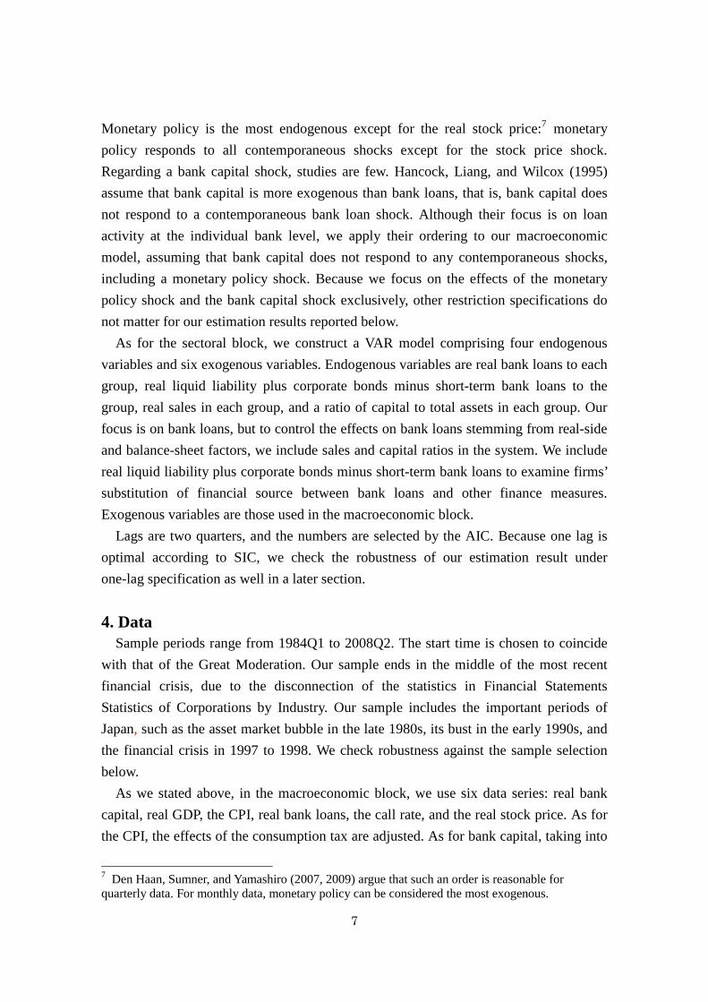
Monetary policy is the most endogenous except for the real stock price:7 monetary

policy responds to all contemporaneous shocks except for the stock price shock.

Regarding a bank capital shock, studies are few. Hancock, Liang, and Wilcox (1995)

assume that bank capital is more exogenous than bank loans, that is, bank capital does

not respond to a contemporaneous bank loan shock. Although their focus is on loan

activity at the individual bank level, we apply their ordering to our macroeconomic

model, assuming that bank capital does not respond to any contemporaneous shocks,

including a monetary policy shock. Because we focus on the effects of the monetary

policy shock and the bank capital shock exclusively, other restriction specifications do

not matter for our estimation results reported below.

As for the sectoral block, we construct a VAR model comprising four endogenous

variables and six exogenous variables. Endogenous variables are real bank loans to each

group, real liquid liability plus corporate bonds minus short-term bank loans to the

group, real sales in each group, and a ratio of capital to total assets in each group. Our

focus is on bank loans, but to control the effects on bank loans stemming from real-side

and balance-sheet factors, we include sales and capital ratios in the system. We include

real liquid liability plus corporate bonds minus short-term bank loans to examine firms’

substitution of financial source between bank loans and other finance measures.

Exogenous variables are those used in the macroeconomic block.

Lags are two quarters, and the numbers are selected by the AIC. Because one lag is

optimal according to SIC, we check the robustness of our estimation result under

one-lag specification as well in a later section.

4. Data

Sample periods range from 1984Q1 to 2008Q2. The start time is chosen to coincide

with that of the Great Moderation. Our sample ends in the middle of the most recent

financial crisis, due to the disconnection of the statistics in Financial Statements

Statistics of Corporations by Industry. Our sample includes the important periods of

Japan, such as the asset market bubble in the late 1980s, its bust in the early 1990s, and

the financial crisis in 1997 to 1998. We check robustness against the sample selection

below.

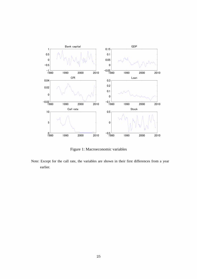
As we stated above, in the macroeconomic block, we use six data series: real bank

capital, real GDP, the CPI, real bank loans, the call rate, and the real stock price. As for

the CPI, the effects of the consumption tax are adjusted. As for bank capital, taking into

7 Den Haan, Sumner, and Yamashiro (2007, 2009) argue that such an order is reasonable for quarterly data. For monthly data, monetary policy can be considered the most exogenous.

8

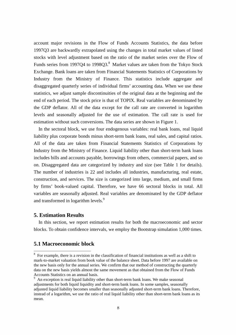
account major revisions in the Flow of Funds Accounts Statistics, the data before

1997Q3 are backwardly extrapolated using the changes in total market values of listed

stocks with level adjustment based on the ratio of the market series over the Flow of

Funds series from 1997Q4 to 1998Q3.8 Market values are taken from the Tokyo Stock

Exchange. Bank loans are taken from Financial Statements Statistics of Corporations by

Industry from the Ministry of Finance. This statistics include aggregate and

disaggregated quarterly series of individual firms’ accounting data. When we use these

statistics, we adjust sample discontinuities of the original data at the beginning and the

end of each period. The stock price is that of TOPIX. Real variables are denominated by

the GDP deflator. All of the data except for the call rate are converted in logarithm

levels and seasonally adjusted for the use of estimation. The call rate is used for

estimation without such conversions. The data series are shown in Figure 1.

In the sectoral block, we use four endogenous variables: real bank loans, real liquid

liability plus corporate bonds minus short-term bank loans, real sales, and capital ratios.

All of the data are taken from Financial Statements Statistics of Corporations by

Industry from the Ministry of Finance. Liquid liability other than short-term bank loans

includes bills and accounts payable, borrowings from others, commercial papers, and so

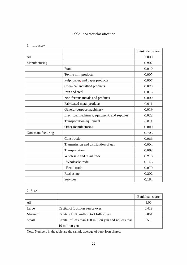
on. Disaggregated data are categorized by industry and size (see Table 1 for details).

The number of industries is 22 and includes all industries, manufacturing, real estate,

construction, and services. The size is categorized into large, medium, and small firms

by firms’ book-valued capital. Therefore, we have 66 sectoral blocks in total. All

variables are seasonally adjusted. Real variables are denominated by the GDP deflator

and transformed in logarithm levels.9

5. Estimation Results In this section, we report estimation results for both the macroeconomic and sector

blocks. To obtain confidence intervals, we employ the Bootstrap simulation 1,000 times.

5.1 Macroeconomic block 8 For example, there is a revision in the classification of financial institutions as well as a shift to mark-to-market valuation from book value of the balance sheet. Data before 1997 are available on the new basis only for the annual series. We confirm that our method of constructing the quarterly data on the new basis yields almost the same movement as that obtained from the Flow of Funds Accounts Statistics on an annual basis. 9 An exception is real liquid liability other than short-term bank loans. We make seasonal adjustments for both liquid liquidity and short-term bank loans. In some samples, seasonally adjusted liquid liability becomes smaller than seasonally adjusted short-term bank loans. Therefore, instead of a logarithm, we use the ratio of real liquid liability other than short-term bank loans as its mean.

9

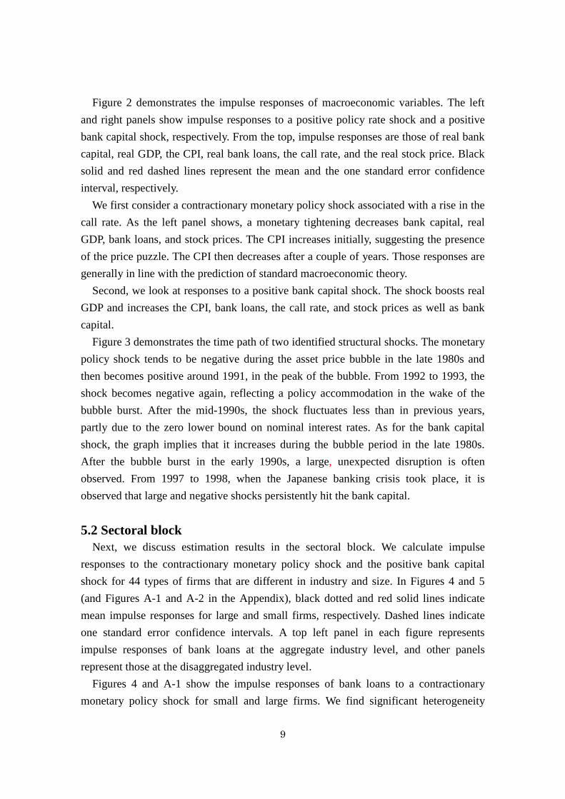
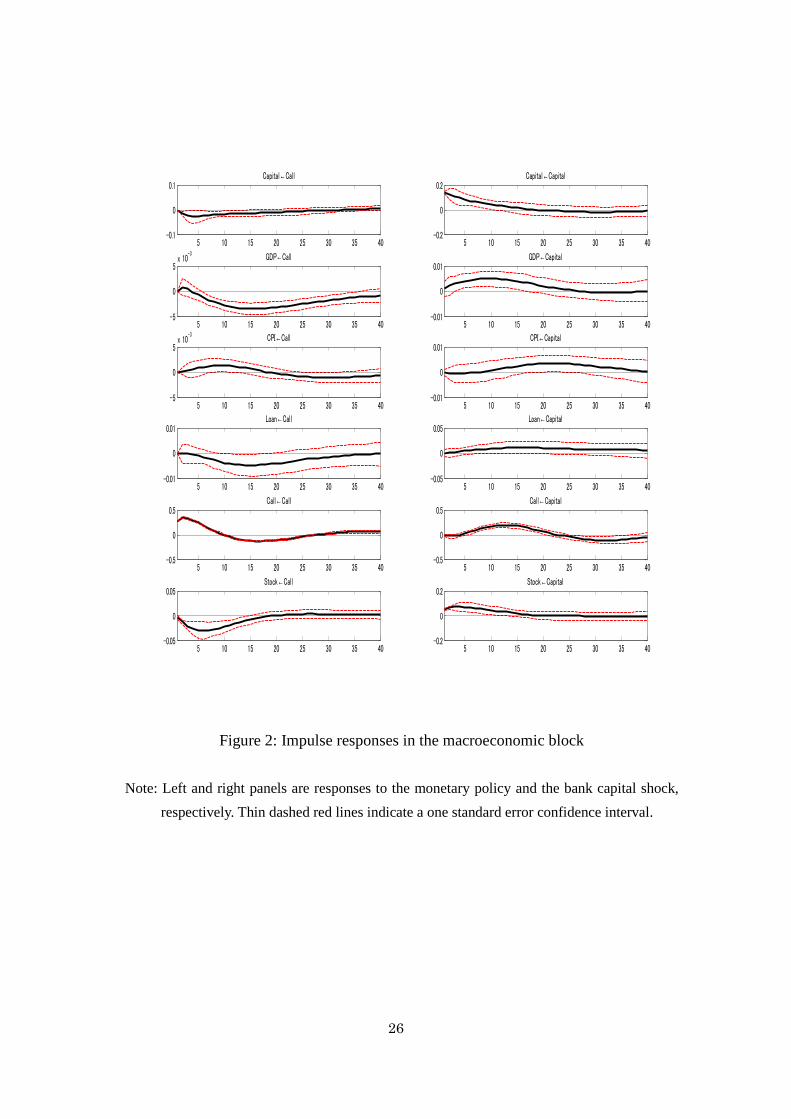
Figure 2 demonstrates the impulse responses of macroeconomic variables. The left

and right panels show impulse responses to a positive policy rate shock and a positive

bank capital shock, respectively. From the top, impulse responses are those of real bank

capital, real GDP, the CPI, real bank loans, the call rate, and the real stock price. Black

solid and red dashed lines represent the mean and the one standard error confidence

interval, respectively.

We first consider a contractionary monetary policy shock associated with a rise in the

call rate. As the left panel shows, a monetary tightening decreases bank capital, real

GDP, bank loans, and stock prices. The CPI increases initially, suggesting the presence

of the price puzzle. The CPI then decreases after a couple of years. Those responses are

generally in line with the prediction of standard macroeconomic theory.

Second, we look at responses to a positive bank capital shock. The shock boosts real

GDP and increases the CPI, bank loans, the call rate, and stock prices as well as bank

capital.

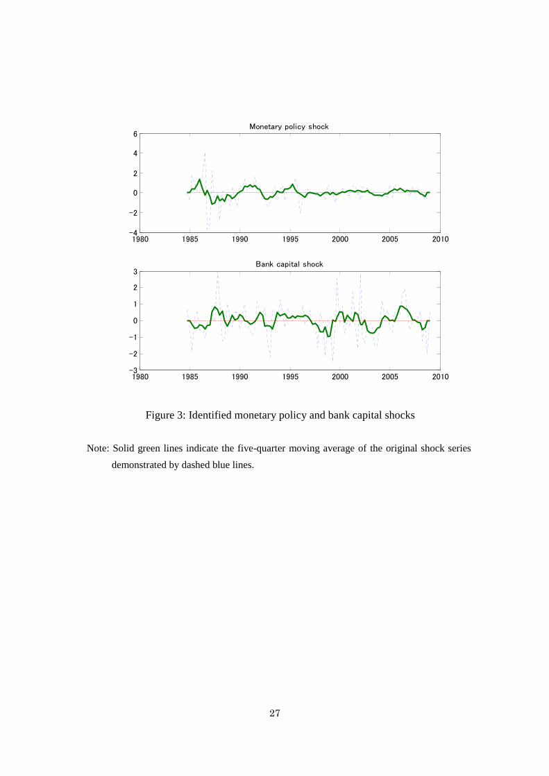
Figure 3 demonstrates the time path of two identified structural shocks. The monetary

policy shock tends to be negative during the asset price bubble in the late 1980s and

then becomes positive around 1991, in the peak of the bubble. From 1992 to 1993, the

shock becomes negative again, reflecting a policy accommodation in the wake of the

bubble burst. After the mid-1990s, the shock fluctuates less than in previous years,

partly due to the zero lower bound on nominal interest rates. As for the bank capital

shock, the graph implies that it increases during the bubble period in the late 1980s.

After the bubble burst in the early 1990s, a large, unexpected disruption is often

observed. From 1997 to 1998, when the Japanese banking crisis took place, it is

observed that large and negative shocks persistently hit the bank capital.

5.2 Sectoral block Next, we discuss estimation results in the sectoral block. We calculate impulse

responses to the contractionary monetary policy shock and the positive bank capital

shock for 44 types of firms that are different in industry and size. In Figures 4 and 5

(and Figures A-1 and A-2 in the Appendix), black dotted and red solid lines indicate

mean impulse responses for large and small firms, respectively. Dashed lines indicate

one standard error confidence intervals. A top left panel in each figure represents

impulse responses of bank loans at the aggregate industry level, and other panels

represent those at the disaggregated industry level.

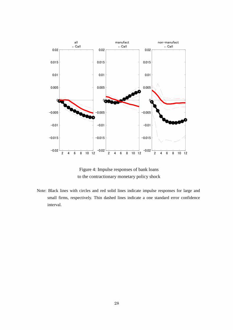
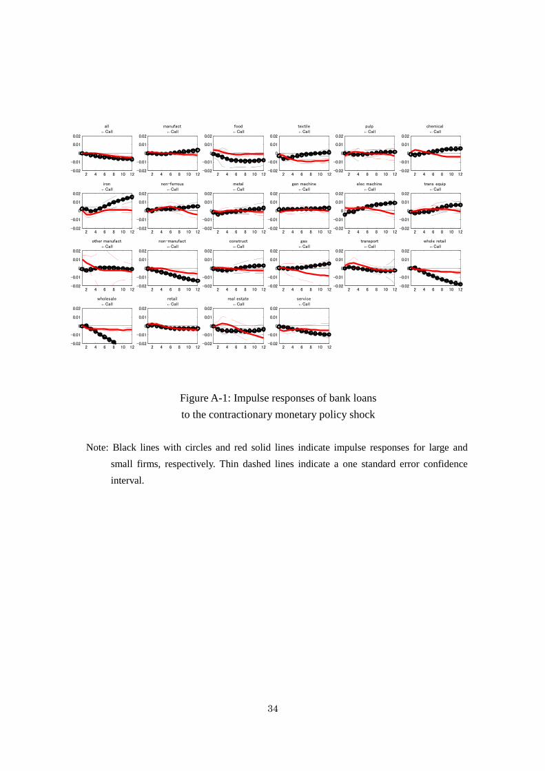
Figures 4 and A-1 show the impulse responses of bank loans to a contractionary

monetary policy shock for small and large firms. We find significant heterogeneity

10

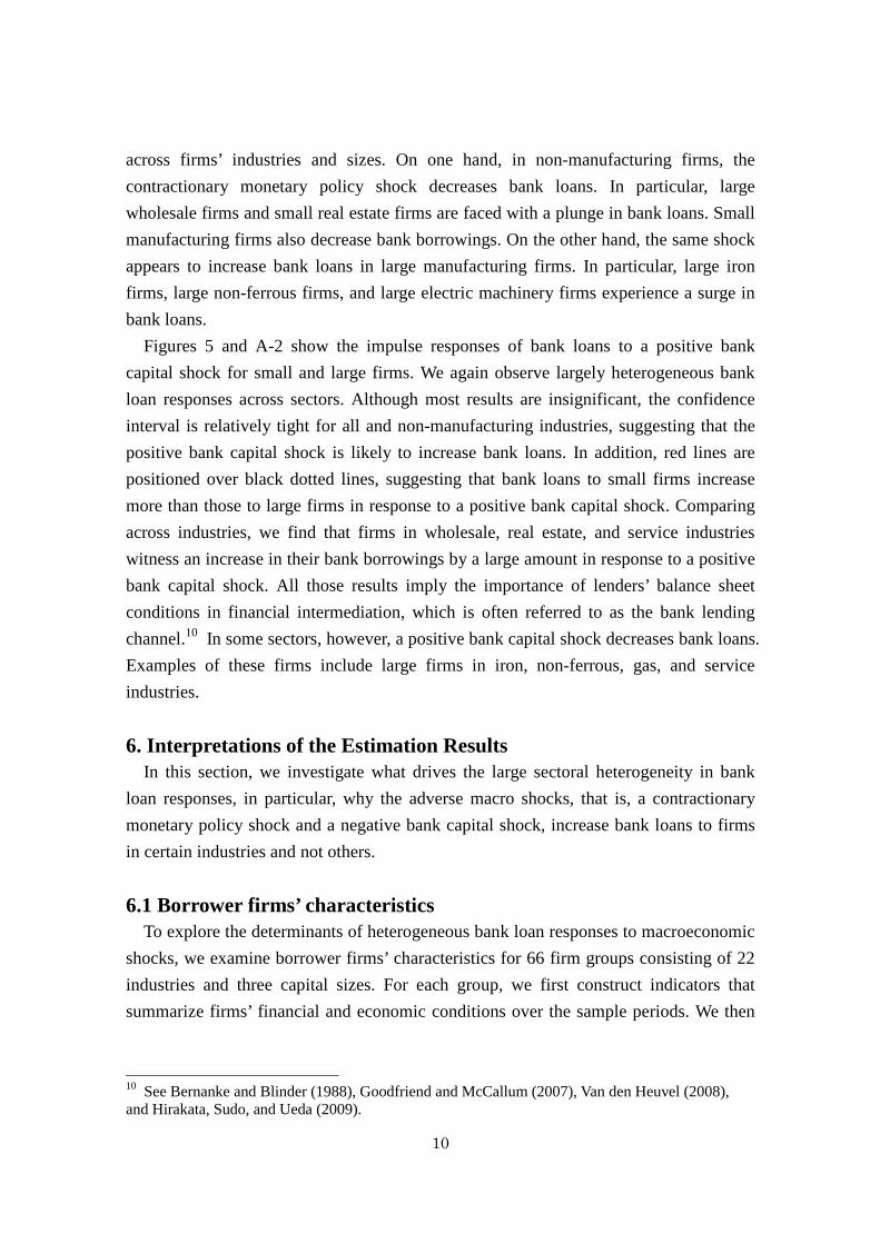
across firms’ industries and sizes. On one hand, in non-manufacturing firms, the

contractionary monetary policy shock decreases bank loans. In particular, large

wholesale firms and small real estate firms are faced with a plunge in bank loans. Small

manufacturing firms also decrease bank borrowings. On the other hand, the same shock

appears to increase bank loans in large manufacturing firms. In particular, large iron

firms, large non-ferrous firms, and large electric machinery firms experience a surge in

bank loans.

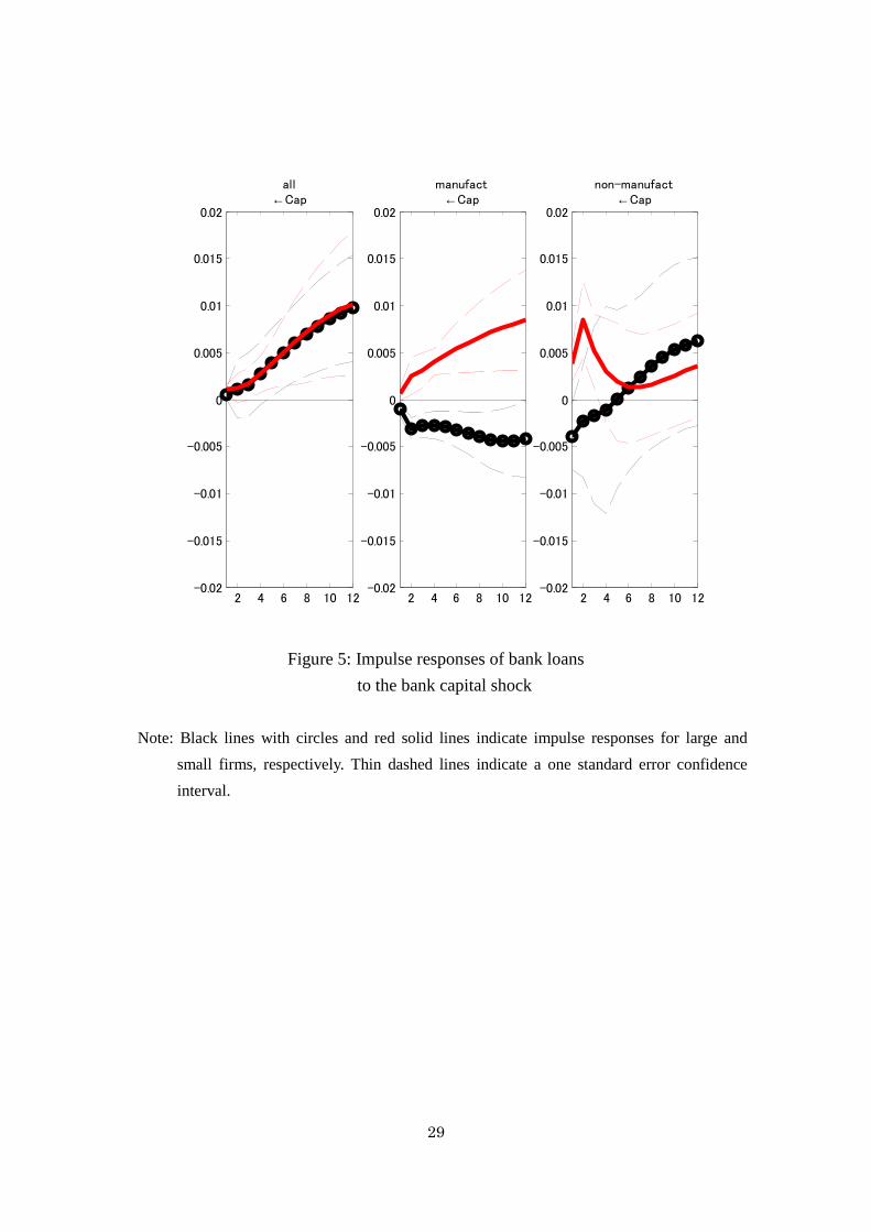
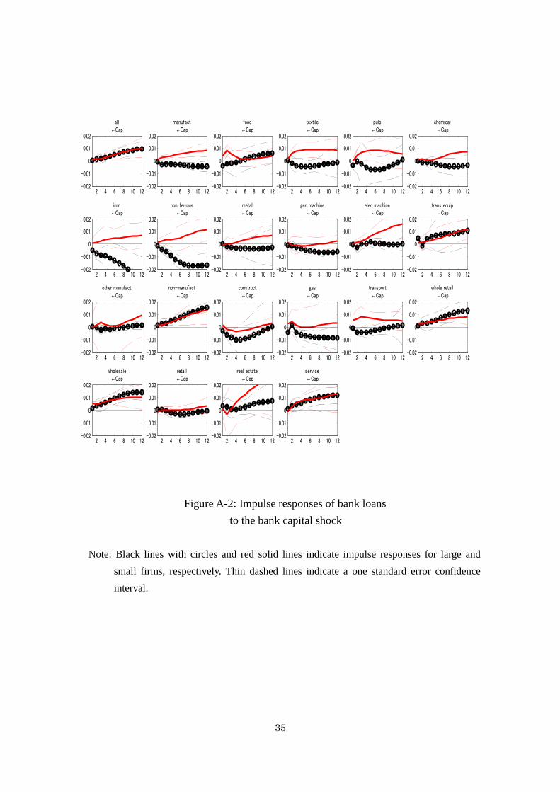
Figures 5 and A-2 show the impulse responses of bank loans to a positive bank

capital shock for small and large firms. We again observe largely heterogeneous bank

loan responses across sectors. Although most results are insignificant, the confidence

interval is relatively tight for all and non-manufacturing industries, suggesting that the

positive bank capital shock is likely to increase bank loans. In addition, red lines are

positioned over black dotted lines, suggesting that bank loans to small firms increase

more than those to large firms in response to a positive bank capital shock. Comparing

across industries, we find that firms in wholesale, real estate, and service industries

witness an increase in their bank borrowings by a large amount in response to a positive

bank capital shock. All those results imply the importance of lenders’ balance sheet

conditions in financial intermediation, which is often referred to as the bank lending

channel.10 In some sectors, however, a positive bank capital shock decreases bank loans.

Examples of these firms include large firms in iron, non-ferrous, gas, and service

industries.

6. Interpretations of the Estimation Results In this section, we investigate what drives the large sectoral heterogeneity in bank

loan responses, in particular, why the adverse macro shocks, that is, a contractionary

monetary policy shock and a negative bank capital shock, increase bank loans to firms

in certain industries and not others.

6.1 Borrower firms’ characteristics To explore the determinants of heterogeneous bank loan responses to macroeconomic

shocks, we examine borrower firms’ characteristics for 66 firm groups consisting of 22

industries and three capital sizes. For each group, we first construct indicators that

summarize firms’ financial and economic conditions over the sample periods. We then

10 See Bernanke and Blinder (1988), Goodfriend and McCallum (2007), Van den Heuvel (2008), and Hirakata, Sudo, and Ueda (2009).

11

examine how those indicators are correlated with the degree of bank loan responses.11

We divide indicators into four categories, each of which bears a different aspect of

economic conditions. The indicators in the first category contain information about

borrower firms’ liability side: the ratio of capital to assets, the ratio of bank borrowings

to assets, and the ratio of corporate bonds to assets.12 As we discussed above, the

importance of borrower firms’ liability conditions is underscored by Gertler and

Gilchrist (1994) and Bernanke, Gertler, and Gilchrist (1999). Gertler and Gilchrist

(1994), in particular, emphasize the importance of accessibility to capital markets. We

employ the indicators as a proxy for such firms’ accessibility to the market. If the

argument in Gertler and Gilchrist (1994) holds true, the ratio of corporate bonds to

assets matters for bank loan responses to the two shocks.

The indicators in the second category are related to the maturity of borrower firms’

finances: the ratio of long-term bank borrowings to assets, the ratio of short-term bank

borrowings to assets, the ratio of cash and deposit holdings to assets, and the ratio of

liquid assets to liquid liabilities. By making use of the second category, we deepen the

analysis regarding the first category and examine whether borrower firms’ liquidity

matters for bank loan responses.

The indicators in the third category capture borrower firms’ flow side: the interest

coverage ratio and the growth rate of sales.13 The interest coverage ratio reflects not

only borrower firms’ profitability but also their liability conditions, and the growth rate

of sales reflects the degree of firms’ economic activity.

The indicators in the final category are related to firms’ inventories: a correlation

between inventory growth and sales growth and the ratio of the standard deviation of

inventory growth to the standard deviation of sales growth. Bernanke and Gertler (1995),

stressing the relationship between inventories and bank loans, argue that in response to

an adverse shock, firms try to finance costs associated with accumulated inventory by

increasing their demand for bank loans if a credit constraint is not stringent; such a

channel accounts for the positive response of bank loans to an adverse shock. To

examine whether a similar mechanism is present in our data series, we include the

aforementioned two variables in our analysis. Suppose that the firms that increase their

demand for bank loans after an adverse shock are likely to increase their inventories in

response to a drop in sales brought about by the shock and that the adjustments to

11 As Rajan and Zingales (1998) point out, a technological difference makes some industries heavily dependent on external finance and other industries not. 12 Other liability variables include trade credits (bills and accounts payable). 13 The interest coverage ratio is defined as the ratio of the sum of operating income and interest income to interest expenses.

12

inventory are quicker than those to sales; then a correlation between inventory growth

and sales growth should be negative, and a ratio of the standard deviation of inventory

growth to the standard deviation of sales growth should be high for that group of firms.

As a correlation between inventory growth and sales growth becomes more negative or

the ratio of the standard deviation of inventory growth relative to that of sales growth

becomes higher, bank loans increase more in response to the contractionary shock and

less in response to the expansionary shock.

To explore the determinants of heterogeneous bank loan responses, we examine how

strongly those indicators regarding borrower firms’ characteristics are correlated with

bank loan responses. Admittedly, these borrower firms’ characteristics may be

endogenously related to how the bank loans respond to economic shocks, and this

analytical approach does not necessarily pin down the causality from borrower firms’

characteristics to bank loan responses. This analysis, however, illustrates the relative

significance of each economic aspect in determining the bank loans.

6.2 Correlations between borrower firms’ characteristics and bank loan responses

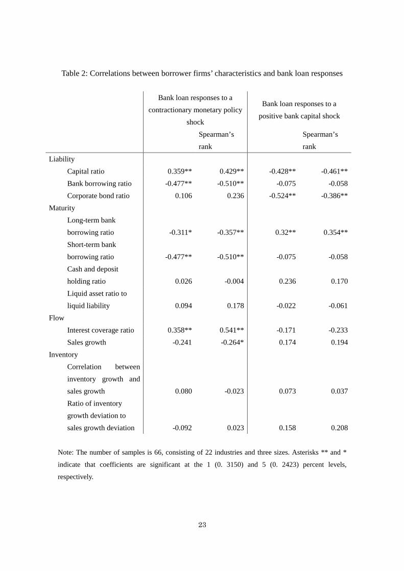
Table 2 provides correlations between the aforementioned firms’ characteristics and

bank loan responses. We choose the cumulative impulse responses (CIRs) of bank loans

up to 12 quarters after shocks as the summary statistics of the bank responses.14 In the

table, the first two and the last two columns indicate correlations regarding responses to

the monetary policy shock and the bank capital shock, respectively. We report two kinds

of correlation: the ordinary correlation and Spearman’s rank correlation, since

Spearman’s rank correlation is robust to outliers. Considering that Figures 4 and 5 have

wide confidence intervals, we mainly focus on the results based on Spearman’s rank

correlation.

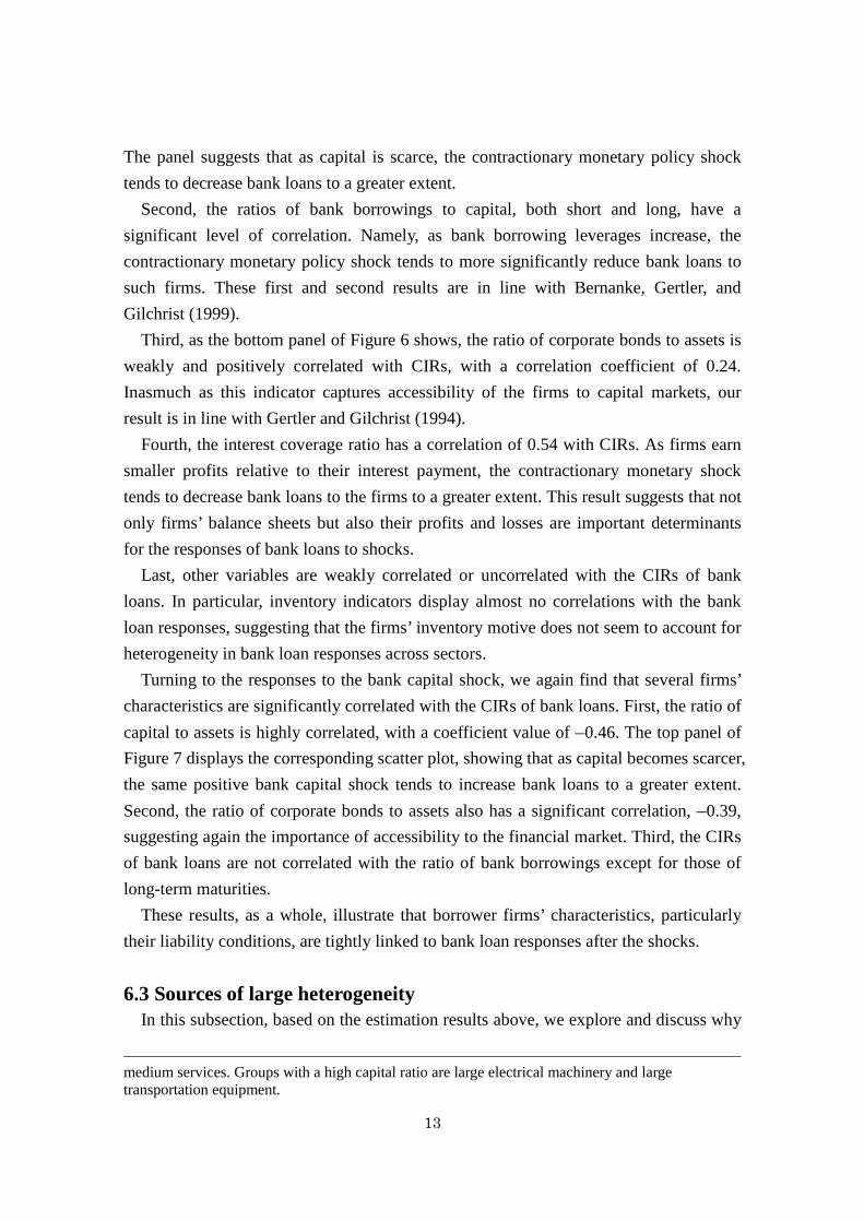
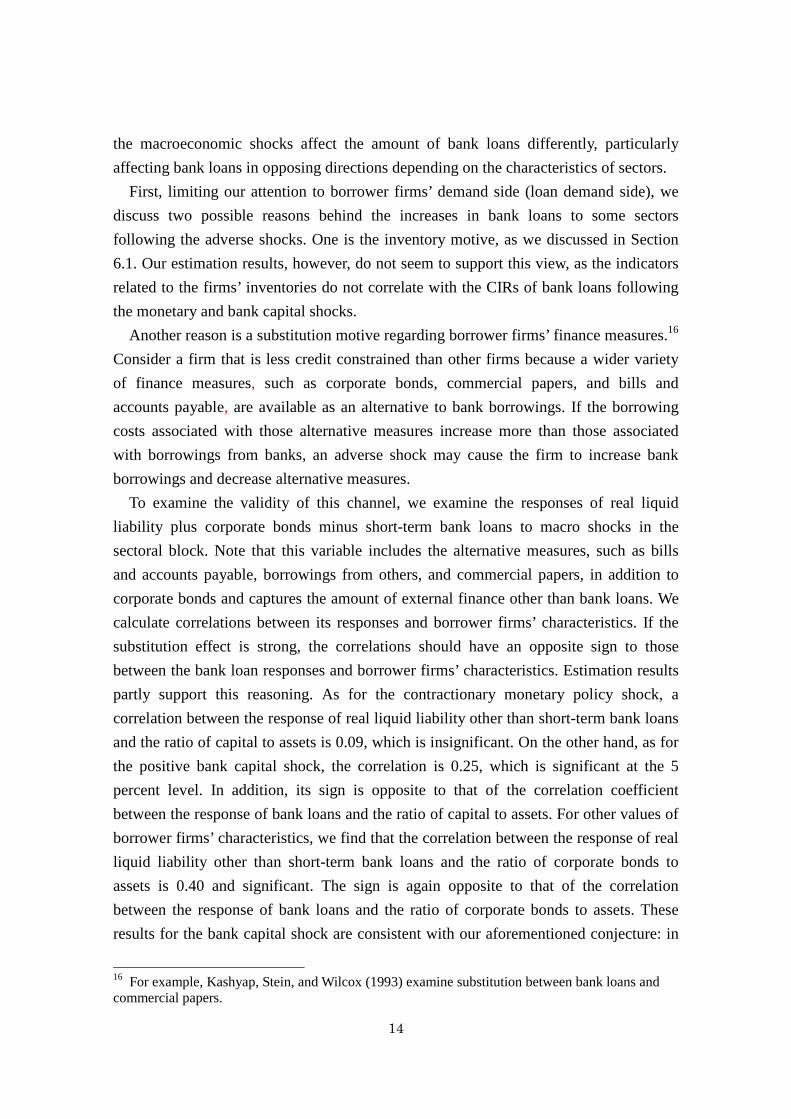
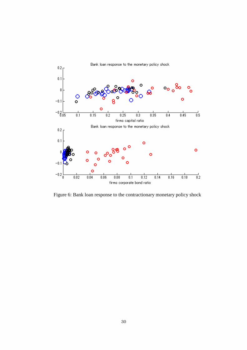
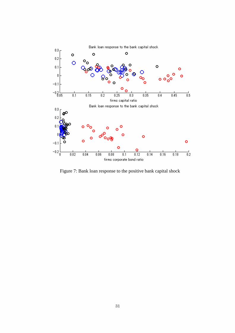
For illustrative purposes, we also plot CIRs and the indicators discussed above in

Figures 6 and 7. A vertical axis indicates the degree of bank loan responses. A horizontal

axis in the top and bottom panels indicates the ratio of capital to assets and the ratio of

corporate bonds to assets, respectively. A large blue circle indicates small firms, and red

and black circles indicate large and medium firms, respectively.

As for the monetary policy shock, we find that several firms’ characteristics are

significantly correlated with the degree of bank loan responses. First, the ratio of capital

to assets has a correlation of 0.43. The top panel of Figure 6 shows its scatter plot.15

14 Changes in the time horizon of 12 quarters do not significantly affect our results. 15 Groups with a low capital ratio are small and medium real estate, medium retail trade, and

13

The panel suggests that as capital is scarce, the contractionary monetary policy shock

tends to decrease bank loans to a greater extent.

Second, the ratios of bank borrowings to capital, both short and long, have a

significant level of correlation. Namely, as bank borrowing leverages increase, the

contractionary monetary policy shock tends to more significantly reduce bank loans to

such firms. These first and second results are in line with Bernanke, Gertler, and

Gilchrist (1999).

Third, as the bottom panel of Figure 6 shows, the ratio of corporate bonds to assets is

weakly and positively correlated with CIRs, with a correlation coefficient of 0.24.

Inasmuch as this indicator captures accessibility of the firms to capital markets, our

result is in line with Gertler and Gilchrist (1994).

Fourth, the interest coverage ratio has a correlation of 0.54 with CIRs. As firms earn

smaller profits relative to their interest payment, the contractionary monetary shock

tends to decrease bank loans to the firms to a greater extent. This result suggests that not

only firms’ balance sheets but also their profits and losses are important determinants

for the responses of bank loans to shocks.

Last, other variables are weakly correlated or uncorrelated with the CIRs of bank

loans. In particular, inventory indicators display almost no correlations with the bank

loan responses, suggesting that the firms’ inventory motive does not seem to account for

heterogeneity in bank loan responses across sectors.

Turning to the responses to the bank capital shock, we again find that several firms’

characteristics are significantly correlated with the CIRs of bank loans. First, the ratio of

capital to assets is highly correlated, with a coefficient value of –0.46. The top panel of

Figure 7 displays the corresponding scatter plot, showing that as capital becomes scarcer,

the same positive bank capital shock tends to increase bank loans to a greater extent.

Second, the ratio of corporate bonds to assets also has a significant correlation, –0.39,

suggesting again the importance of accessibility to the financial market. Third, the CIRs

of bank loans are not correlated with the ratio of bank borrowings except for those of

long-term maturities.

These results, as a whole, illustrate that borrower firms’ characteristics, particularly

their liability conditions, are tightly linked to bank loan responses after the shocks.

6.3 Sources of large heterogeneity In this subsection, based on the estimation results above, we explore and discuss why

medium services. Groups with a high capital ratio are large electrical machinery and large transportation equipment.

14

the macroeconomic shocks affect the amount of bank loans differently, particularly

affecting bank loans in opposing directions depending on the characteristics of sectors.

First, limiting our attention to borrower firms’ demand side (loan demand side), we

discuss two possible reasons behind the increases in bank loans to some sectors

following the adverse shocks. One is the inventory motive, as we discussed in Section

6.1. Our estimation results, however, do not seem to support this view, as the indicators

related to the firms’ inventories do not correlate with the CIRs of bank loans following

the monetary and bank capital shocks.

Another reason is a substitution motive regarding borrower firms’ finance measures.16

Consider a firm that is less credit constrained than other firms because a wider variety

of finance measures, such as corporate bonds, commercial papers, and bills and

accounts payable, are available as an alternative to bank borrowings. If the borrowing

costs associated with those alternative measures increase more than those associated

with borrowings from banks, an adverse shock may cause the firm to increase bank

borrowings and decrease alternative measures.

To examine the validity of this channel, we examine the responses of real liquid

liability plus corporate bonds minus short-term bank loans to macro shocks in the

sectoral block. Note that this variable includes the alternative measures, such as bills

and accounts payable, borrowings from others, and commercial papers, in addition to

corporate bonds and captures the amount of external finance other than bank loans. We

calculate correlations between its responses and borrower firms’ characteristics. If the

substitution effect is strong, the correlations should have an opposite sign to those

between the bank loan responses and borrower firms’ characteristics. Estimation results

partly support this reasoning. As for the contractionary monetary policy shock, a

correlation between the response of real liquid liability other than short-term bank loans

and the ratio of capital to assets is 0.09, which is insignificant. On the other hand, as for

the positive bank capital shock, the correlation is 0.25, which is significant at the 5

percent level. In addition, its sign is opposite to that of the correlation coefficient

between the response of bank loans and the ratio of capital to assets. For other values of

borrower firms’ characteristics, we find that the correlation between the response of real

liquid liability other than short-term bank loans and the ratio of corporate bonds to

assets is 0.40 and significant. The sign is again opposite to that of the correlation

between the response of bank loans and the ratio of corporate bonds to assets. These

results for the bank capital shock are consistent with our aforementioned conjecture: in

16 For example, Kashyap, Stein, and Wilcox (1993) examine substitution between bank loans and commercial papers.

15

the wake of a shock, bank borrowings and alternative measures of finance are close

substitutes.

In summary, among borrowers’ demand side (loan demand side) factors, the firms’

substitution motive between bank loans and alternative financial measures explains a

portion of sectoral heterogeneity in the response of bank loans to a bank capital shock at

a statistically significant level. The motive, however, does not seem to provide a full

explanation for the heterogeneity, because the heterogeneous responses across sectors to

a monetary policy shock are not explained by this factor.

Therefore, it is possible to argue that large heterogeneity of bank loan responses,

particularly those to a monetary policy shock, may be attributed to a loan supply side,

such as banks’ maturity conditions, profitability conditions, and balance sheet

conditions. As Den Haan, Sumner, and Yamashiro (2007, 2009) discuss, the changes in

banks’ maturity misalignment or balance sheet conditions following macroeconomic

shocks may affect their loan portfolio decisions, leading to changes in bank loans across

sectors. Along this line, Aoki and Sudo (2012) investigate the banks’ portfolio decisions

and show that banks under the value at risk constraint choose to hold less risky assets

whenever their balance sheets are deteriorating.

6.4 Sample periods: the effects of (de)regulation and zero lower bound Japan’s financial markets and financial system experienced drastic changes in the late

1980s and early 1990s.17 Two changes are worth noting. First, the BIS agreement in

1988 required banks to hold a sound amount of bank capital. Combined with the asset

market bubble and its burst around 1990, the bank capital requirement started to play an

important role in banks’ loan behaviors from the early 1990s. Second, corporate bond

issuance became available as a finance tool in the late 1980s and early 1990s. In the late

1970s, the bond issue criteria were so stringent that only two companies (Toyota Auto

and Matsushita Electric) were qualified to issue corporate bonds. Stringent regulation of

corporate bond issuance was relaxed gradually.

Those changes in economic environments around the bank loans suggest that bank

loan responses to shocks may differ greatly before and after the 1980s. We conjecture

that bank capital shocks mattered less. Accessibility to capital markets, captured by the

ratio of corporate bonds to assets, also mattered less.

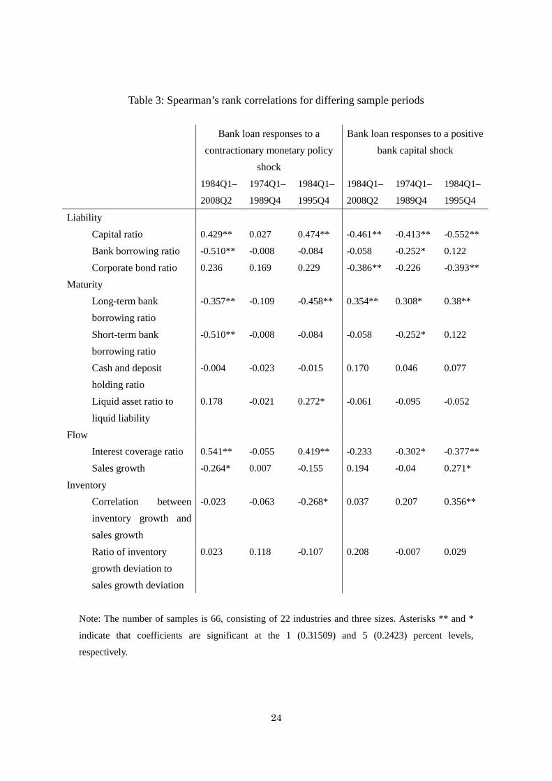
Table 2 reports correlations, showing some validity of our conjectures. In the former

period of 1974Q1 to 1989Q4, the corporate bond ratio is uncorrelated with the degree of

bank loan responses, although the capital ratio still is correlated with the degree of bank

17 See Hoshi and Kashyap (1999) for detail.

16

loan responses.18

Another important issue associated with sample length is the presence of the zero

lower bound of nominal interest rates. As Figure 1 shows, the short-term nominal

interest rate reached almost zero in 1995 and has stayed at that level thereafter. The

non-linearity stemming from the zero lower bound poses a serious challenge to

accurately estimating the monetary policy shock. To check the robustness of our result

from this viewpoint, we therefore estimate the model using the sample period up until

1995Q4. Table 2 shows that our results are not significantly changed from the baseline

result.

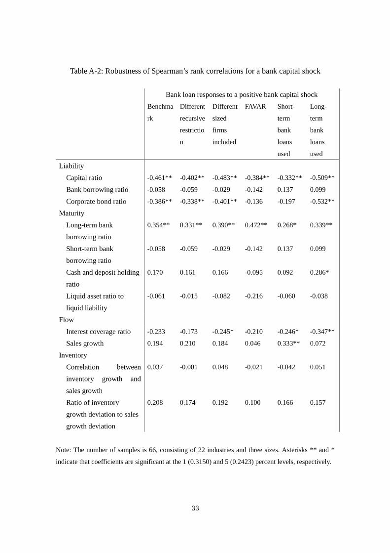
6.5 Robustness

We check the robustness of our results by conducting several model modifications.

Among our results, we focus on correlations between the degree of bank loan responses

and liability conditions. Tables A-1 and A-2 are the summary of the following

robustness check. They report Spearman’s rank correlations for a monetary policy shock

and a bank capital shock, respectively.

First, we impose different recursive restrictions in identifying the two

macroeconomic shocks. We replace our baseline ordering of shocks with the recursive

restriction proposed by Bayoumi (2001). In this setting, the call rate does not respond to

a contemporaneous shock to either the real bank capital or real bank loan. Furthermore,

considering that our real bank capital series contains contemporaneous information on

the financial market price as it is constructed in such a way as to reflect the

contemporaneous movement of banks’ stock prices, we assume that the real bank capital

is the most endogenous next to the real stock price. As the second column of Tables A-1

and A-2 shows, the obtained correlations under this setting hardly change from the

baseline.

Second, we examine whether incorporating linkages across sectors affects the

estimation results. Note that in the benchmark estimation, a sectoral block consists of

only one sector with the same industry and of the same firm size. We here add the real

sales of the same industry but different firm size to each sectoral block, considering that

linkages among the same industry but across different firm sizes are stronger than those

across industries. The third column of Tables A-1 and A-2 shows the robustness of the

previous results.

Third, to check the robustness against the number of lags, we estimate the model with

18 No correlation implies two possibilities: either macro shocks do not influence bank loans, or the degree of bank loan responses is independent of borrower firms’ characteristics.

17

lags of one quarter. Although we do not report it in the table, the obtained correlations

hardly change.

Fourth, to check the robustness against the number of variables and the way to extract

the monetary policy shock and the bank capital shock, we use a Factor-Augmented VAR

approach (FAVAR) as in Bernanke et al. (2005) and Favero et al. (2005). By making use

of the macroeconomic factor, we reduce the number of variables in the macroeconomic

block (X1t) from six to three: real aggregate bank capital, a macroeconomic factor, and

the call rate. The macroeconomic factor is the first principal component extracted from

a set of economic variables (Mt) for which the detail is given in the Appendix, and the

whole FAVAR is specified as follows:

ttt eXLM +Ω= 1)( ,

ttt uXLAX 111 )( += .

Identification assumptions and lag orders for the macroeconomic block and the sectoral

block are the same as in the baseline model.

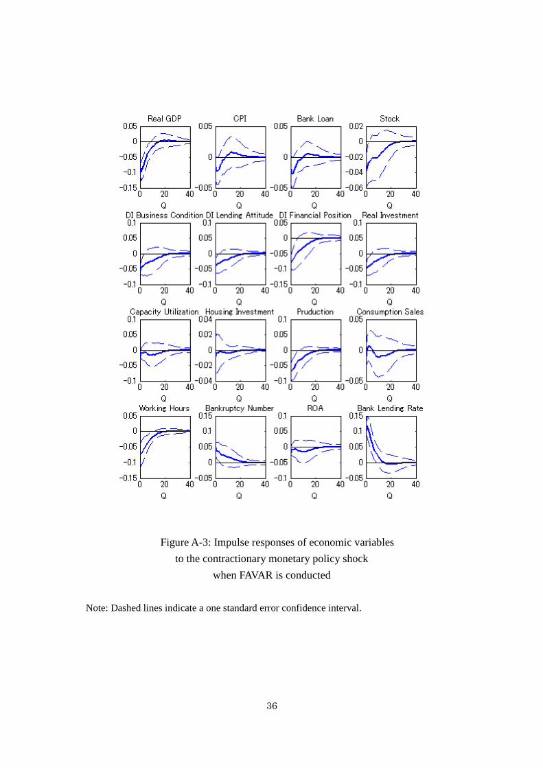
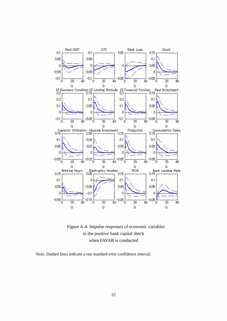
Results are reported in Figures A-3 and A-4 and Tables A-1 and A-2. First, Figures

A-3 and A-4 show the responses of selected macroeconomic variables to the

contractionary monetary policy shock and the positive bank capital shock, respectively.

The general pattern of macroeconomic response that is obtained under the baseline

model is maintained and further enriched by the responses of other variables—such as

production, investment, and unemployment—that are not included in the baseline model.

The fourth column of Tables A-1 and A-2 reports correlations between the degree of

bank loan responses and liability conditions. Our bottom-line results are intact:

borrower firms’ liability conditions are tightly linked to the bank loan responses.

However, we find some differences from the baseline model and the FAVAR model. For

the monetary policy shock, the capital ratio and the interest coverage ratio of borrower

firms are uncorrelated with the degree of bank loan responses. For the bank capital

shock, the corporate bond ratio is uncorrelated with the degree of bank loans.

Finally, we distinguish long-term bank loans from short-term bank loans. In the

benchmark model, we have used total bank loans. We replace them by either short-term

or long-term bank loans and estimate the model in the same way otherwise. The fifth

and last columns of Tables A-1 and A-2 reveal that the responses of long-term bank

loans are more highly correlated with the borrower firms’ characteristics than those of

short-term bank loans.

7. Conclusion

In this paper, we investigated the determinants of bank loan responses to shocks to

18

monetary policy and bank capital based on borrower firms’ data at a disaggregated level.

Using the bank loan series disaggregated by the borrower firms’ size and industry, we

first estimated the bank loan responses by the block recursive VAR proposed by Davis

and Haltiwanger (2001). The bank loan responses display a substantial heterogeneity

across sectors. Next, to see the determinants of the heterogeneity, we constructed

several indicators of borrower firms’ characteristics, including those associated with

their balance sheet conditions and inventories, and examined the statistical relationship

between the bank loan responses and those indicators. We found that borrower firms’

characteristics, particularly their liability conditions, are tightly linked to the bank loan

responses and that inventory-related variables that are stressed in the existing studies are

not linked with the bank loan responses. In addition, we found that a portion of

heterogeneity accounted for by the borrower firms’ liability condition is limited. In

particular, our results do not answer a question regarding why the macroeconomic

shocks change bank loans in opposing directions across sectors.

In this respect, deeper analyses on banks’ portfolio decisions are called for from both

empirical and theoretical perspectives. From an empirical viewpoint, analyses based on

the bank loan series disaggregated by bank types, such as city bank, regional bank, and

regional bank II, in Japan that differ in terms of size, maturity arrangements, and

regulatory capital requirements, would be a promising avenue because it may

disentangle the determinants of bank loan portfolios associated with the lender banks’

side from those associated with the borrower firms’ side. Along this line, Hancock et al.

(1995), using the U.S. data, report that the size of the bank matters in regard to how the

bank loan changes after the bank capital shock. From a theoretical viewpoint, a model

that at least incorporates both credit-constrained firms and credit-constrained banks is

needed.

Our results have policy implications, particularly in regard to those undertaken during

Japan’s lost decade. In that era, the Bank of Japan continued its accommodative

monetary policy, and the Japanese government injected capital to banks to strengthen

the banks’ balance sheets. According to the bank loan responses to monetary policy

shocks and bank capital shocks obtained in the current analysis, the outcomes of these

policies may have been increases in bank loans to non-manufacturing firms such as

construction and real estate industries, substituting out the loans from manufacturing

firms. A possible consequence of such shift in bank loans may be the misallocation of

bank credits through ever-greening or zombie-lending, as discussed by Sekine,

Kobayashi, and Saita (2003); Peek and Rosengren (2005); and Caballero, Hoshi, and

Kashyap (2008). The analysis of that channel, however, is left for the future research.

19

ReferencesReferencesReferencesReferences

Acemoglu, Daron, Vasco M. Carvalho, Asuman Ozdaglar, and Alireza Tahbaz-Salehi

(2012) “The Network Origins of Aggregate Fluctuations,” Econometrica, 80(5),

1977–2016.

Aoki, Kosuke, and Nao Sudo (2012) “Asset Portfolio Choice of Banks and Inflation

Dynamics,” Bank of Japan Working Paper Series, 12-E-5.

Bayoumi, Tamim (2001) “The Morning After: Explaining the Slowdown in Japanese

Growth in the 1990s,” Journal of International Economics, 53, 241–259.

Bernanke, Ben S., and Alan Blinder (1988) “Credit, Money and Aggregate Demand,”

American Economic Review, 78, 435–439.

Bernanke, Ben S., and Mark Gertler (1995) “Inside the Black Box: the Credit Channel

of Monetary Policy Transmission,” Journal of Economic Perspectives, 9, 27–48.

Bernanke, Ben S., Mark Gertler, and Simon Gilchrist (1999) “The Financial Accelerator

in a Quantitative Business Cycle Framework,” in Handbook of Macroeconomics, J.

B. Taylor and M. Woodford (eds.), Vol. 1, chapter 21, pp. 1341–1393.

Bernanke, Ben S., J. Boivin, and P. Eliasz (2005) “Measuring the Effects of Monetary

Policy: A Factor-Augmented Vector Autoregressive (FAVAR) Approach,” Quarterly

Journal of Economics, 120(1), 387–422.

Caballero, Ricardo J., Takeo Hoshi, and Anil K. Kashyap (2008) “Zombie Lending and

Depressed Restructuring in Japan,” American Economic Review, 98(5), 1943–1977.

Carlino, Gerald, and Robert Defina (1998) “The Differential Regional Effects of

Monetary Policy,” Review of Economics and Statistics, 80(4), 572–587.

Covas, Francisco, and Wouter J. Den Haan (2007) “Cyclical Behavior of Debt and

Equity Using a Panel of Canadian Firms,” Bank of Canada Working Paper, 2007-44.

Davis, S. J., and J. Haltiwanger (2001) “Sectoral Job Creation and Destruction

Responses to Oil Price Changes,” Journal of Monetary Economics, 48(3), 465–512.

Den Haan, Wouter J., Steven W. Sumner, and Guy M. Yamashiro (2007) “Bank Loan

Portfolios and the Monetary Transmission Mechanism,” Journal of Monetary

Economics, 54, 904–924.

Den Haan, Wouter J., Steven W. Sumner, and Guy M. Yamashiro (2009) “Bank Loan

Portfolios and the Canadian Monetary Transmission Mechanism,” Canadian

Journal of Economics, 42(3), 1150–1175.

Favero, Carlo A., M. Marcellino, and F. Neglia (2005) “Principal Components at Work:

The Empirical Analysis of Monetary Policy with Large Data Sets,” Journal of

Applied Econometrics, 20, 603–620.

20

Foerster, Andrew, Pierre-Daniel G. Sarte, and Mark W. Watson (2011) “Sectoral versus

Aggregate Shocks: A Structural Factor Analysis of Industrial Production,” Journal

of Political Economy, 19(1), 1–38.

Gabaix, Xavier (2011) “The Granular Origins of Aggregate Fluctuations,”

Econometrica, 79, 733–772.

Gertler, Mark, and Simon Gilchrist (1993) “The Role of Credit Market Imperfections in

the Monetary Transmission Mechanism: Arguments and Evidence,” Scandinavian

Journal of Economics, 95, 43–64.

Gertler, Mark, and Simon Gilchrist (1994) “Monetary Policy, Business Cycles, and the

Behavior of Small Manufacturing Firms,” Quarterly Journal of Economics, 109(2),

309–340.

Goodfriend, Marvin, and Bennett T. McCallum (2007) “Banking and Interest Rates in

Monetary Policy Analysis: A Quantitative Exploration,” Journal of Monetary

Economics, 54(5), 1480–1507.

Hancock, Diana, Andrew J. Laing, and James A. Wilcox (1995) “Bank Capital Shocks:

Dynamic Effects on Securities, Loans, and Capital,” Journal of Banking and

Finance, 19, 661–677.

Hirakata, Naohisa, Nao Sudo, and Kozo Ueda (2009) “Chained Credit Contracts and

Financial Accelerators,” IMES Discussion Paper 2009-E-30, Institute for Monetary

and Economic Studies, Bank of Japan.

Hirakata, Naohisa, Nao Sudo, and Kozo Ueda (2010) “Japan’s Banking Crisis and Lost

Decades,” mimeo.

Hirakata, Naohisa, Nao Sudo, and Kozo Ueda (2011) “Do Banking Shocks Matter for

the U.S. Economy?” Journal of Economic Dynamics and Control, 35(12),

2042–2063.

Hoshi, Takeo, and Anil K. Kashyap (1999) “The Japanese Banking Crisis: Where Did It

Come From and How Will It End?” NBER Macroeconomics Annual, 14, 129–212.

Kashyap, Anil K., Jeremy C. Stein, and David W. Wilcox (1993) “Monetary Policy and

Credit Conditions: Composition of External Finance,” American Economic Review,

83(1), 78–98.

Kashyap, Anil K., Owen A. Lamont, and Jeremy C. Stein (1994) “Credit Conditions and

the Cyclical Behavior of Inventories,” Quarterly Journal of Economics, 109(3),

565–592.

Kilian, L. (1998) “Small-Sample Confidence Intervals for Impulse Response

Functions,” Review of Economics and Statistics, 80(2), 218–230.

Lee, K., and S. Ni (2002) “On the Dynamic Effects of Oil Price Shocks: A Study Using

21

Industry Level Data,” Journal of Monetary Economics, 49(4), 823–852.

Miyao, Ryuzo (2002) “The Effects of Monetary Policy in Japan,” Journal of Money,

Credit and Banking, 34(2), 376–392.

Mora, N., and Andrew Logan (2010) “Shocks to Bank Capital: Evidence from UK

Banks at Home and Away,” Bank of England Working Paper No. 387.

Morgan, Donald P. (1994) “The Credit Effects of Monetary Policy: Evidence Using

Loan Commitments,” Journal of Money, Credit and Banking, 30(1), 102–118.

Peek, Joe, and Eric S. Rosengren (1997) “The International Transmission of Financial

Shocks: Case of Japan,” American Economic Review, 87(4), 625–638.

Peek, Joe, and Eric S. Rosengren (2000) “Collateral Damage: Effects of the Japanese

Bank Crisis on Real Activity in the United States,” American Economic Review,

90(1), 30–45.

Peek, Joe, and Eric S. Rosengren (2005) “Unnatural Selection: Perverse Incentives and

the Misallocation of Credit in Japan,” American Economic Review, 95(4),

1144–1166.

Rajan, Raghuram G., and Luigi Zingales (1998) “Financial Dependence and Growth,”

American Economic Review, 88(3), 559–586.

Sekine, Toshitaka, Keiichiro Kobayashi, and Yumi Saita (2003) “Forbearance Lending:

The Case of Japanese Firms,” Monetary and Economic Studies, 21(2), 69–92.

Sims, Christopher A. (1992) “Interpreting the Macroeconomic Time Series Facts: The

Effects of Monetary Policy,” European Economic Review, 36, 975–1011.

Sims, Christopher A., and Tao Zha (2006) “Does Monetary Policy Generate

Recessions?” Macroeconomic Dynamics, 10, 231–272.

Van den Heuvel, Skander J. (2008) “The Welfare Cost of Bank Capital Requirements,”

Journal of Monetary Economics, 55(2), 298–320.

22

Table 1: Sector classification

1. Industry

Bank loan share

All 1.000

Manufacturing 0.207

Food 0.019

Textile mill products 0.005

Pulp, paper, and paper products 0.007

Chemical and allied products 0.023

Iron and steel 0.015

Non-ferrous metals and products 0.009

Fabricated metal products 0.011

General-purpose machinery 0.019

Electrical machinery, equipment, and supplies 0.022

Transportation equipment 0.011

Other manufacturing 0.020

Non-manufacturing 0.796

Construction 0.066

Transmission and distribution of gas 0.004

Transportation 0.062

Wholesale and retail trade 0.216

Wholesale trade 0.146

Retail trade 0.070

Real estate 0.202

Services 0.164

2. Size

Bank loan share

All 1.00

Large Capital of 1 billion yen or over 0.422

Medium Capital of 100 million to 1 billion yen 0.064

Small Capital of less than 100 million yen and no less than

10 million yen

0.513

Note: Numbers in the table are the sample average of bank loan shares.

23

Table 2: Correlations between borrower firms’ characteristics and bank loan responses

Bank loan responses to a

contractionary monetary policy

shock


positive bank capital shock

Spearman’s

rank

Spearman’s

rank

Liability

Capital ratio 0.359** 0.429** -0.428** -0.461**

Bank borrowing ratio -0.477** -0.510** -0.075 -0.058

Corporate bond ratio 0.106 0.236 -0.524** -0.386**

Maturity

Long-term bank

borrowing ratio -0.311* -0.357** 0.32** 0.354**

Short-term bank

borrowing ratio -0.477** -0.510** -0.075 -0.058

Cash and deposit

holding ratio 0.026 -0.004 0.236 0.170

Liquid asset ratio to

liquid liability 0.094 0.178 -0.022 -0.061

Flow

Interest coverage ratio 0.358** 0.541** -0.171 -0.233

Sales growth -0.241 -0.264* 0.174 0.194

Inventory

Correlation between

inventory growth and

sales growth 0.080 -0.023 0.073 0.037

Ratio of inventory

growth deviation to

sales growth deviation -0.092 0.023 0.158 0.208

Note: The number of samples is 66, consisting of 22 industries and three sizes. Asterisks ** and *

indicate that coefficients are significant at the 1 (0. 3150) and 5 (0. 2423) percent levels,

respectively.

24

Table 3: Spearman’s rank correlations for differing sample periods


contractionary monetary policy

shock

Bank loan responses to a positive

bank capital shock

1984Q1–

2008Q2

1974Q1–

1989Q4

1984Q1–

1995Q4

1984Q1–

2008Q2

1974Q1–

1989Q4

1984Q1–

1995Q4

Liability

Capital ratio 0.429** 0.027 0.474** -0.461** -0.413** -0.552**

Bank borrowing ratio -0.510** -0.008 -0.084 -0.058 -0.252* 0.122

Corporate bond ratio 0.236 0.169 0.229 -0.386** -0.226 -0.393**

Maturity

Long-term bank

borrowing ratio

-0.357** -0.109 -0.458** 0.354** 0.308* 0.38**

Short-term bank

borrowing ratio

-0.510** -0.008 -0.084 -0.058 -0.252* 0.122

Cash and deposit

holding ratio

-0.004 -0.023 -0.015 0.170 0.046 0.077


liquid liability

0.178 -0.021 0.272* -0.061 -0.095 -0.052

Flow

Interest coverage ratio 0.541** -0.055 0.419** -0.233 -0.302* -0.377**

Sales growth -0.264* 0.007 -0.155 0.194 -0.04 0.271*

Inventory

Correlation between


sales growth

-0.023 -0.063 -0.268* 0.037 0.207 0.356**

Ratio of inventory

growth deviation to

sales growth deviation

0.023 0.118 -0.107 0.208 -0.007 0.029


indicate that coefficients are significant at the 1 (0.31509) and 5 (0.2423) percent levels,

respectively.

25

1980 1990 2000 2010

-1

-0.5

0

0.5

1

Bank capital

1980 1990 2000 2010

-0.05

0

0.05

0.1

0.15

GDP

1980 1990 2000 2010

-0.02

0

0.02

0.04

CPI

1980 1990 2000 2010

-0.1

0

0.1

0.2

0.3

Loan

1980 1990 2000 2010

0

5

10

Call rate

1980 1990 2000 2010

-0.5

0

0.5

Stock

Figure 1: Macroeconomic variables

Note: Except for the call rate, the variables are shown in their first differences from a year

earlier.

26

Figure 2: Impulse responses in the macroeconomic block

Note: Left and right panels are responses to the monetary policy and the bank capital shock,

respectively. Thin dashed red lines indicate a one standard error confidence interval.

5 10 15 20 25 30 35 40

-0.1

0

0.1

Capital←Call

5 10 15 20 25 30 35 40

-0.2

0

0.2

Capital←Capital

5 10 15 20 25 30 35 40

-5

0

5

x 10

-3

GDP←Call

5 10 15 20 25 30 35 40

-0.01

0

0.01

GDP←Capital

5 10 15 20 25 30 35 40

-5

0

5

x 10

-3

CPI←Call

5 10 15 20 25 30 35 40

-0.01

0

0.01

CPI←Capital

5 10 15 20 25 30 35 40

-0.01

0

0.01

Loan←Call

5 10 15 20 25 30 35 40

-0.05

0

0.05

Loan←Capital

5 10 15 20 25 30 35 40

-0.5

0

0.5

Call←Call

5 10 15 20 25 30 35 40

-0.5

0

0.5

Call←Capital

5 10 15 20 25 30 35 40

-0.05

0

0.05

Stock←Call

5 10 15 20 25 30 35 40

-0.2

0

0.2

Stock←Capital

27

1980 1985 1990 1995 2000 2005 2010

-4

-2

0

2

4

6

Monetary policy shock

1980 1985 1990 1995 2000 2005 2010

-3

-2

-1

0

1

2

3

Bank capital shock

Figure 3: Identified monetary policy and bank capital shocks

Note: Solid green lines indicate the five-quarter moving average of the original shock series

demonstrated by dashed blue lines.

28

2 4 6 8 10 12

-0.02

-0.015

-0.01

-0.005

0

0.005

0.01

0.015

0.02

all

←Call

2 4 6 8 10 12

-0.02

-0.015

-0.01

-0.005

0

0.005

0.01

0.015

0.02

manufact

←Call

2 4 6 8 10 12

-0.02

-0.015

-0.01

-0.005

0

0.005

0.01

0.015

0.02

non-manufact

←Call

Figure 4: Impulse responses of bank loans

to the contractionary monetary policy shock

Note: Black lines with circles and red solid lines indicate impulse responses for large and

small firms, respectively. Thin dashed lines indicate a one standard error confidence

interval.

29

2 4 6 8 10 12

-0.02

-0.015

-0.01

-0.005

0

0.005

0.01

0.015

0.02

all

←Cap

2 4 6 8 10 12

-0.02

-0.015

-0.01

-0.005

0

0.005

0.01

0.015

0.02

manufact

←Cap

2 4 6 8 10 12

-0.02

-0.015

-0.01

-0.005

0

0.005

0.01

0.015

0.02

non-manufact

←Cap

Figure 5: Impulse responses of bank loans

to the bank capital shock



interval.

30

Figure 6: Bank loan response to the contractionary monetary policy shock

31

Figure 7: Bank loan response to the positive bank capital shock

32

Table A-1: Robustness of Spearman’s rank correlations for a monetary policy shock

Bank loan responses to a contractionary monetary policy shock

Benchma

rk

Different

recursive

restrictio

n

Different

sized

firms

included

FAVAR Short-

term

bank

loans

used

Long-

term

bank

loans

used

Liability

Capital ratio 0.429** 0.341** 0.489** -0.037 0.287* 0.550**

Bank borrowing ratio -0.510** -0.571** -0.446** -0.381** -0.171 -0.380**

Corporate bond ratio 0.236 0.165 0.237 -0.209 0.056 0.353**

Maturity

Long-term bank

borrowing ratio

-0.357** -0.294* -0.375** 0.025 -0.417** -0.331**

Short-term bank

borrowing ratio

-0.510** -0.571** -0.446** -0.381** -0.171 -0.380**

Cash and deposit holding

ratio

-0.004 -0.017 0.051 0.051 0.212 -0.073


liquid liability

0.178 0.127 0.244* -0.060 0.296* 0.214

Flow

Interest coverage ratio 0.541** 0.525** 0.529** 0.136 0.200 0.563**

Sales growth -0.264* -0.247* -0.353** -0.181 -0.251* -0.099

Inventory

Correlation between


sales growth

-0.023 0.000 -0.014 0.160 -0.043 0.059

Ratio of inventory

growth deviation to sales

growth deviation

0.023 0.084 -0.015 0.000 -0.170 -0.032


indicate that coefficients are significant at the 1 (0.31359) and 5 (0.24203) percent levels,

respectively.

33

Table A-2: Robustness of Spearman’s rank correlations for a bank capital shock

Bank loan responses to a positive bank capital shock

Benchma

rk

Different

recursive

restrictio

n

Different

sized

firms

included

FAVAR Short-

term

bank

loans

used

Long-

term

bank

loans

used

Liability

Capital ratio -0.461** -0.402** -0.483** -0.384** -0.332** -0.509**

Bank borrowing ratio -0.058 -0.059 -0.029 -0.142 0.137 0.099

Corporate bond ratio -0.386** -0.338** -0.401** -0.136 -0.197 -0.532**

Maturity

Long-term bank

borrowing ratio

0.354** 0.331** 0.390** 0.472** 0.268* 0.339**

Short-term bank

borrowing ratio

-0.058 -0.059 -0.029 -0.142 0.137 0.099

Cash and deposit holding

ratio

0.170 0.161 0.166 -0.095 0.092 0.286*


liquid liability

-0.061 -0.015 -0.082 -0.216 -0.060 -0.038

Flow

Interest coverage ratio -0.233 -0.173 -0.245* -0.210 -0.246* -0.347**

Sales growth 0.194 0.210 0.184 0.046 0.333** 0.072

Inventory

Correlation between


sales growth

0.037 -0.001 0.048 -0.021 -0.042 0.051

Ratio of inventory

growth deviation to sales

growth deviation

0.208 0.174 0.192 0.100 0.166 0.157


indicate that coefficients are significant at the 1 (0.3150) and 5 (0.2423) percent levels, respectively.

34

Figure A-1: Impulse responses of bank loans




interval.

2 4 6 8 10 12

-0.02

-0.01

0

0.01

0.02

all

←Call

2 4 6 8 10 12

-0.02

-0.01

0

0.01

0.02

manufact

←Call

2 4 6 8 10 12

-0.02

-0.01

0

0.01

0.02

food

←Call

2 4 6 8 10 12

-0.02

-0.01

0

0.01

0.02

textile

←Call

2 4 6 8 10 12

-0.02

-0.01

0

0.01

0.02

pulp

←Call

2 4 6 8 10 12

-0.02

-0.01

0

0.01

0.02

chemical

←Call

2 4 6 8 10 12

-0.02

-0.01

0

0.01

0.02

iron

←Call

2 4 6 8 10 12

-0.02

-0.01

0

0.01

0.02

non-ferrous

←Call

2 4 6 8 10 12

-0.02

-0.01

0

0.01

0.02

metal

←Call

2 4 6 8 10 12

-0.02

-0.01

0

0.01

0.02

gen machine

←Call

2 4 6 8 10 12

-0.02

-0.01

0

0.01

0.02

elec machine

←Call

2 4 6 8 10 12

-0.02

-0.01

0

0.01

0.02

trans equip

←Call

2 4 6 8 10 12

-0.02

-0.01

0

0.01

0.02

other manufact

←Call

2 4 6 8 10 12

-0.02

-0.01

0

0.01

0.02

non-manufact

←Call

2 4 6 8 10 12

-0.02

-0.01

0

0.01

0.02

construct

←Call

2 4 6 8 10 12

-0.02

-0.01

0

0.01

0.02

gas

←Call

2 4 6 8 10 12

-0.02

-0.01

0

0.01

0.02

transport

←Call

2 4 6 8 10 12

-0.02

-0.01

0

0.01

0.02

whole retail

←Call

2 4 6 8 10 12

-0.02

-0.01

0

0.01

0.02

wholesale

←Call

2 4 6 8 10 12

-0.02

-0.01

0

0.01

0.02

retail

←Call

2 4 6 8 10 12

-0.02

-0.01

0

0.01

0.02

real estate

←Call

2 4 6 8 10 12

-0.02

-0.01

0

0.01

0.02

service

←Call

35

Figure A-2: Impulse responses of bank loans

to the bank capital shock



interval.

2 4 6 8 10 12

-0.02

-0.01

0

0.01

0.02

all

←Cap

2 4 6 8 10 12

-0.02

-0.01

0

0.01

0.02

manufact

←Cap

2 4 6 8 10 12

-0.02

-0.01

0

0.01

0.02

food

←Cap

2 4 6 8 10 12

-0.02

-0.01

0

0.01

0.02

textile

←Cap

2 4 6 8 10 12

-0.02

-0.01

0

0.01

0.02

pulp

←Cap

2 4 6 8 10 12

-0.02

-0.01

0

0.01

0.02

chemical

←Cap

2 4 6 8 10 12

-0.02

-0.01

0

0.01

0.02

iron

←Cap

2 4 6 8 10 12

-0.02

-0.01

0

0.01

0.02

non-ferrous

←Cap

2 4 6 8 10 12

-0.02

-0.01

0

0.01

0.02

metal

←Cap

2 4 6 8 10 12

-0.02

-0.01

0

0.01

0.02

gen machine

←Cap

2 4 6 8 10 12

-0.02

-0.01

0

0.01

0.02

elec machine

←Cap

2 4 6 8 10 12

-0.02

-0.01

0

0.01

0.02

trans equip

←Cap

2 4 6 8 10 12

-0.02

-0.01

0

0.01

0.02

other manufact

←Cap

2 4 6 8 10 12

-0.02

-0.01

0

0.01

0.02

non-manufact

←Cap

2 4 6 8 10 12

-0.02

-0.01

0

0.01

0.02

construct

←Cap

2 4 6 8 10 12

-0.02

-0.01

0

0.01

0.02

gas

←Cap

2 4 6 8 10 12

-0.02

-0.01

0

0.01

0.02

transport

←Cap

2 4 6 8 10 12

-0.02

-0.01

0

0.01

0.02

whole retail

←Cap

2 4 6 8 10 12

-0.02

-0.01

0

0.01

0.02

wholesale

←Cap

2 4 6 8 10 12

-0.02

-0.01

0

0.01

0.02

retail

←Cap

2 4 6 8 10 12

-0.02

-0.01

0

0.01

0.02

real estate

←Cap

2 4 6 8 10 12

-0.02

-0.01

0

0.01

0.02

service

←Cap

36

Figure A-3: Impulse responses of economic variables


when FAVAR is conducted

Note: Dashed lines indicate a one standard error confidence interval.

37

Figure A-4: Impulse responses of economic variables

to the positive bank capital shock

when FAVAR is conducted

Note: Dashed lines indicate a one standard error confidence interval.

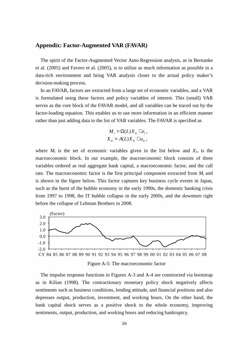
38

Appendix: Factor-Augmented VAR (FAVAR)

The spirit of the Factor-Augmented Vector Auto-Regression analysis, as in Bernanke

et al. (2005) and Favero et al. (2005), is to utilize as much information as possible in a

data-rich environment and bring VAR analysis closer to the actual policy maker’s

decision-making process.

In an FAVAR, factors are extracted from a large set of economic variables, and a VAR

is formulated using these factors and policy variables of interest. This (small) VAR

serves as the core block of the FAVAR model, and all variables can be traced out by the

factor-loading equation. This enables us to use more information in an efficient manner

rather than just adding data to the list of VAR variables. The FAVAR is specified as

ttt eXLM +Ω= 1)( ,

ttt uXLAX 111 )( += ,

where Mt is the set of economic variables given in the list below and X1t is the

macroeconomic block. In our example, the macroeconomic block consists of three

variables ordered as real aggregate bank capital, a macroeconomic factor, and the call

rate. The macroeconomic factor is the first principal component extracted from Mt and

is shown in the figure below. This factor captures key business cycle events in Japan,

such as the burst of the bubble economy in the early 1990s, the domestic banking crisis

from 1997 to 1998, the IT bubble collapse in the early 2000s, and the downturn right

before the collapse of Lehman Brothers in 2008.

-2.0

-1.0

0.0

1.0

2.0

3.0

84 85 86 87 88 89 90 91 92 93 94 95 96 97 98 99 00 01 02 03 04 05 06 07 08

(Factor)

CY

Figure A-5: The macroeconomic factor

The impulse response functions in Figures A-3 and A-4 are constructed via bootstrap

as in Kilian (1998). The contractionary monetary policy shock negatively affects

sentiments such as business conditions, lending attitude, and financial positions and also

depresses output, production, investment, and working hours. On the other hand, the

bank capital shock serves as a positive shock to the whole economy, improving

sentiments, output, production, and working hours and reducing bankruptcy.

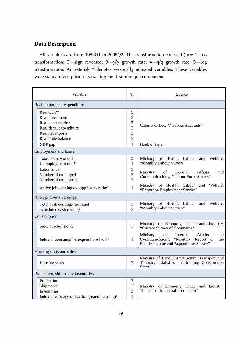
39

Data Description

All variables are from 1984Q1 to 2008Q2. The transformation codes (T.) are 1—no

transformation; 2—sign reversed; 3—y/y growth rate; 4—q/q growth rate; 5—log

transformation. An asterisk * denotes seasonally adjusted variables. These variables

were standardized prior to extracting the first principle component.

Variable T. Source

Real output, real expenditures

Real GDP* Real investment Real consumption Real fiscal expenditure Real net exports Real trade balance

5 3 3 3 3 3

Cabinet Office, “National Accounts”

GDP gap 1 Bank of Japan

Employment and hours

Total hours worked Unemployment rate*

3 1

Ministry of Health, Labour and Welfare, “Monthly Labour Survey”

Labor force Number of employed Number of employees

3 3 3

Ministry of Internal Affairs and Communications, “Labour Force Survey”

Active job openings-to-applicants ratio* 1 Ministry of Health, Labour and Welfare, “Report on Employment Service”

Average hourly earnings

Total cash earnings (nominal) Scheduled cash earnings

3 3

Ministry of Health, Labour and Welfare, “Monthly Labour Survey”

Consumption

Sales at retail stores 3

Ministry of Economy, Trade and Industry, “Current Survey of Commerce”

Index of consumption expenditure level* 1 Ministry of Internal Affairs and Communications, “Monthly Report on the Family Income and Expenditure Survey”

Housing starts and sales

Housing starts 3

Ministry of Land, Infrastructure, Transport and Tourism, “Statistics on Building Construction Starts”

Production, shipments, inventories

Production Shipments Inventories Index of capacity utilization (manufacturing)*

3 3 3 1

Ministry of Economy, Trade and Industry, “Indices of Industrial Production”

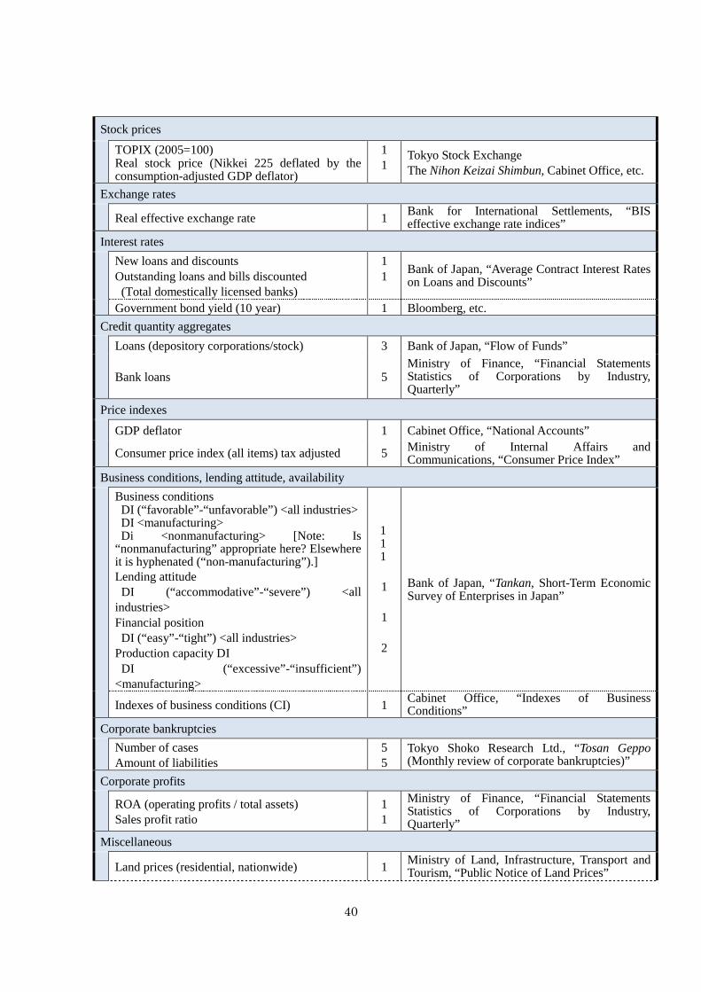
40

Stock prices

TOPIX (2005=100) Real stock price (Nikkei 225 deflated by the consumption-adjusted GDP deflator)

1 1

Tokyo Stock Exchange The Nihon Keizai Shimbun, Cabinet Office, etc.

Exchange rates

Real effective exchange rate 1 Bank for International Settlements, “BIS effective exchange rate indices”

Interest rates

New loans and discounts Outstanding loans and bills discounted (Total domestically licensed banks)

1 1

Bank of Japan, “Average Contract Interest Rates on Loans and Discounts”

Government bond yield (10 year) 1 Bloomberg, etc.

Credit quantity aggregates

Loans (depository corporations/stock) 3 Bank of Japan, “Flow of Funds”

Bank loans 5 Ministry of Finance, “Financial Statements Statistics of Corporations by Industry, Quarterly”

Price indexes

GDP deflator 1 Cabinet Office, “National Accounts”

Consumer price index (all items) tax adjusted 5 Ministry of Internal Affairs and Communications, “Consumer Price Index”

Business conditions, lending attitude, availability

Business conditions DI (“favorable”-“unfavorable”) <all industries> DI <manufacturing> Di <nonmanufacturing> [Note: Is

“nonmanufacturing” appropriate here? Elsewhere it is hyphenated (“non-manufacturing”).] Lending attitude DI (“accommodative”-“severe”) <all

industries> Financial position DI (“easy”-“tight”) <all industries>

Production capacity DI DI (“excessive”-“insufficient”)

<manufacturing>

1 1 1 1 1 2

Bank of Japan, “Tankan, Short-Term Economic Survey of Enterprises in Japan”

Indexes of business conditions (CI) 1 Cabinet Office, “Indexes of Business Conditions”

Corporate bankruptcies

Number of cases Amount of liabilities

5 5

Tokyo Shoko Research Ltd., “Tosan Geppo (Monthly review of corporate bankruptcies)”

Corporate profits

ROA (operating profits / total assets) Sales profit ratio

1 1

Ministry of Finance, “Financial Statements Statistics of Corporations by Industry, Quarterly”

Miscellaneous

Land prices (residential, nationwide) 1 Ministry of Land, Infrastructure, Transport and Tourism, “Public Notice of Land Prices”

41

Oil prices (WTI, Dubai) 1 Bloomberg Real GDP (U.S.) Consumer price index (U.S., all items)

4 3

BEA BLS

Heterogeneous Bank Loan Responses to Monetary … Bank Loan Responses to Monetary Policy and Bank...

Documents

Transcript of Heterogeneous Bank Loan Responses to Monetary … Bank Loan Responses to Monetary Policy and Bank...