Herded Gibbs Sampling

Luke BornnHarvard University

bornn@stat.harvard.edu

Yutian ChenUC Irvine

yutian.chen@uci.edu

Nando de FreitasUBC

nando@cs.ubc.ca

Mareija EskelinUBC

mareija@cs.ubc.ca

Jing FangFacebook

jingf@cs.ubc.ca

Max WellingUniversity of Amsterdamwelling@ics.uci.edu

Abstract

The Gibbs sampler is one of the most popular algorithms for inference in statisticalmodels. In this paper, we introduce a herding variant of this algorithm, calledherded Gibbs, that is entirely deterministic. We prove that herded Gibbs has anO(1/T ) convergence rate for models with independent variables and for fullyconnected probabilistic graphical models. Herded Gibbs is shown to outperformGibbs in the tasks of image denoising with MRFs and named entity recognitionwith CRFs. However, the convergence for herded Gibbs for sparsely connectedprobabilistic graphical models is still an open problem.

1 Introduction

Over the last 60 years, we have witnessed great progress in the design of randomized samplingalgorithms; see for example [16, 9, 3, 22] and the references therein. In contrast, the design of deter-ministic algorithms for “sampling” from distributions is still in its inception [8, 13, 7, 20]. There are,however, many important reasons for pursuing this line of attack on the problem. From a theoreti-cal perspective, this is a well defined mathematical challenge whose solution might have importantconsequences. It also brings us closer to reconciling the fact that we typically use pseudo-randomnumber generators to run Monte Carlo algorithms on classical, Von Neumann architecture, comput-ers. Moreover, the theory for some of the recently proposed deterministic sampling algorithms hastaught us that they can achieve O(1/T ) convergence rates [8, 13], which are much faster than thestandard Monte Carlo rates of O(1/

√T ) for computing ergodic averages. From a practical perspec-

tive, the design of deterministic sampling algorithms creates an opportunity for researchers to applya great body of knowledge on optimization to the problem of sampling; see for example [4] for anearly example of this.

The domain of application of currently existing deterministic sampling algorithms is still very nar-row. Importantly, there do not exist deterministic tools for sampling from unnormalized multivariateprobability distributions. This is very limiting because the problem of sampling from unnormalizeddistributions is at the heart of the field of Bayesian inference and the probabilistic programmingapproach to artificial intelligence [17, 6, 18, 11]. At the same time, despite great progress in MonteCarlo simulation, the celebrated Gibbs sampler continues to be one of the most widely-used algo-rithms. For, example it is the inference engine behind popular statistics packages [17], several toolsfor text analysis [21], and Boltzmann machines [2, 12]. The popularity of Gibbs stems from itssimplicity of implementation and the fact that it is a very generic algorithm.

Without any doubt, it would be remarkable if we could design generic deterministic Gibbs sam-plers with fast (theoretical and empirical) rates of convergence. In this paper, we take steps toward

Authors are listed in alphabetical order.

1

arX

iv:1

301.

4168

v2 [

cs.L

G]

16

Mar

201

3

achieving this goal by capitalizing on a recent idea for deterministic simulation known as herding.Herding [24, 23, 10] is a deterministic procedure for generating samples x ∈ X ⊆ Rn, such that theempirical moments µ of the data are matched. The herding procedure, at iteration t, is as follows:

x(t) = argmaxx∈X

〈w(t−1),φ(x)〉

w(t) = w(t−1) + µ− φ(x(t)), (1)

where φ : X → H is a feature map (statistic) from X to a Hilbert spaceH with inner product 〈·, ·〉,w ∈ H is the vector of parameters, and µ ∈ H is the moment vector (expected value of φ overthe data) that we want to match. If we choose normalized features by making ‖φ(x)‖ constant forall x, then the update to generate samples x(t) for t = 1, 2, . . . , T in Equation 1 is equivalent tominimizing the objective

J(x1, . . . ,xT ) =

∥∥∥∥∥µ− 1

T

T∑t=1

φ(x(t))

∥∥∥∥∥2

, (2)

where T may have no prior known value and ‖ · ‖ =√〈·, ·〉 is the naturally defined norm based

upon the inner product of the spaceH [8, 4].

Herding can be used to produce samples from normalized probability distributions. This is doneas follows. Let µ denote a discrete, normalized probability distribution, with µi ∈ [0, 1] and∑ni=1 µi = 1. A natural feature in this case is the vector φ(x) that has all entries equal to zero,

except for the entry at the position indicated by x. For instance, if x = 2 and n = 5, we haveφ(x) = (0, 1, 0, 0, 0)T . Hence, µ = T−1

∑Tt=1 φ(x

(t)) is an empirical estimate of the distribution.In this case, one step of the herding algorithm involves finding the largest component of the weightvector (i? = argmaxi∈{1,2,...,n}w

(t−1)i ), setting x(t) = i?, fixing the i?-entry of φ(x(t)) to one

and all other entries to zero, and updating the weight vector: w(t) = w(t−1) + (µ− φ(x(t))). Theoutput is a set of samples {x(1), . . . , x(T )} for which the empirical estimate µ converges on thetarget distribution µ as O(1/T ).

The herding method, as described thus far, only applies to normalized distributions or to problemswhere the objective is not to guarantee that the samples come from the right target, but to ensure thatsome moments are matched. An interpretation of herding in terms of Bayesian quadrature has beenput forward recently by [14].

In this paper, we will show that it is possible to use herding to generate samples from more complexunnormalized probability distributions. In particular, we introduce a deterministic variant of thepopular Gibbs sampling algorithm, which we refer to as herded Gibbs. While Gibbs relies on draw-ing samples from the full-conditionals at random, herded Gibbs generates the samples by matchingthe full-conditionals. That is, one simply applies herding to all the full-conditional distributions.

The experiments will demonstrate that the new algorithm outperforms Gibbs sampling and meanfield methods in the domain of sampling from sparsely connected probabilistic graphical models,such as grid-lattice Markov random fields (MRFs) for image denoising and conditional randomfields (CRFs) for natural language processing.

We advance the theory by proving that the deterministic Gibbs algorithm converges for distributionsof independent variables and fully-connected probabilistic graphical models. However, a proof es-tablishing suitable conditions that ensure convergence of herded Gibbs sampling for sparsely con-nected probabilistic graphical models is still unavailable.

2 Herded Gibbs Sampling

For a graph of discrete nodes G = (V,E), where the set of nodes are the random variables V ={Xi}Ni=1, Xi ∈ X , let π denote the target distribution defined on G.

Gibbs sampling is one of the most popular methods to draw samples from π. Gibbs alternates (eithersystematically or randomly) the sampling of each variable Xi given XN (i) = xN (i), where i is theindex of the node, and N (i) denotes the neighbors of node i. That is, Gibbs generates each samplefrom its full-conditional distribution p(Xi|xN (i)).

2

Algorithm 1 Herded Gibbs Sampling.

Input: T .Step 1: Set t = 0. Initialize X(0) in the support of π and w(0)

i,xN(i)in (π(Xi = 1|xN (i)) −

1, π(Xi = 1|xN (i))).for t = 1→ T do

Step 2: Pick a node i according to some policy. Denote w = w(t−1)i,x

(t−1)

N(i)

.

Step 3: If w > 0, set x(t)i = 1, otherwise set x(t)i = 0.Step 4: Update weight w(t)

i,x(t)

N(i)

= w(t−1)i,x

(t−1)

N(i)

+ π(Xi = 1|x(t−1)N (i) )− x

(t)i

Step 5: Keep the values of all the other nodes x(t)j = x(t−1)j ,∀j 6= i and all the other weights

w(t)j,xN(j)

= w(t−1)j,xN(j)

,∀j 6= i or xN (j) 6= x(t−1)N (i) .

end forOutput: x(1), . . . ,x(T )

Herded Gibbs replaces the sampling from full-conditionals with herding at the level of the full-conditionals. That is, it alternates a process of matching the full-conditional distributions p(Xi =xi|XN (i)). To do this, herded Gibbs defines a set of auxiliary weights {wi,xN(i)

} for any value ofXi = xi and XN (i) = xN (i). For ease of presentation, we assume the domain of Xi is binary,X = {0, 1}, and we use one weight for every i and assignment to the neighbors xN (i). HerdedGibbs can be trivially generalized to the multivariate setting by employing weight vectors in R|X |instead of scalars.

If the binary variableXi has four binary neighbors XN (i), we must maintain 24 = 16 weight vectors.Only the weight vector corresponding to the current instantiation of the neighbors is updated, asillustrated in Algorithm 1. The memory complexity of herded Gibbs is exponential in the maximumnode degree. Note the algorithm is a deterministic Markov process with state (X,W).

The initialization in step 1 guarantees that X(t) always remains in the support of π. For a deter-ministic scan policy in step 2, we take the value of variables x(tN), t ∈ N as a sample sequence.Throughout the paper all experiments employ a fixed variable traversal for sample generation. Wecall one such traversal of the variables a sweep.

3 Analysis

As herded Gibbs sampling is a deterministic algorithm, there is no stationary probability distributionof states. Instead, we examine the average of the sample states over time and hypothesize that itconverges to the joint distribution, our target distribution, π. To make the treatment precise, we needthe following definition:

Definition 1. For a graph of discrete nodes G = (V,E), where the set of nodes V = {Xi}Ni=1,Xi ∈ X , P (τ)

T is the empirical estimate of the joint distribution obtained by averaging over Tsamples acquired from G. P (τ)

T is derived from T samples, collected at the end of every sweep overN variables, starting from the τ th sweep:

P(τ)T (X = x) =

1

T

τ+T−1∑k=τ

I(X(kN) = x) (3)

Our goal is to prove that the limiting average sample distribution over time converges to the targetdistribution π. Specifically, we want to show the following:

limT→∞

P(τ)T (x) = π(x),∀τ ≥ 0 (4)

If this holds, we also want to know what the convergence rate is.

3

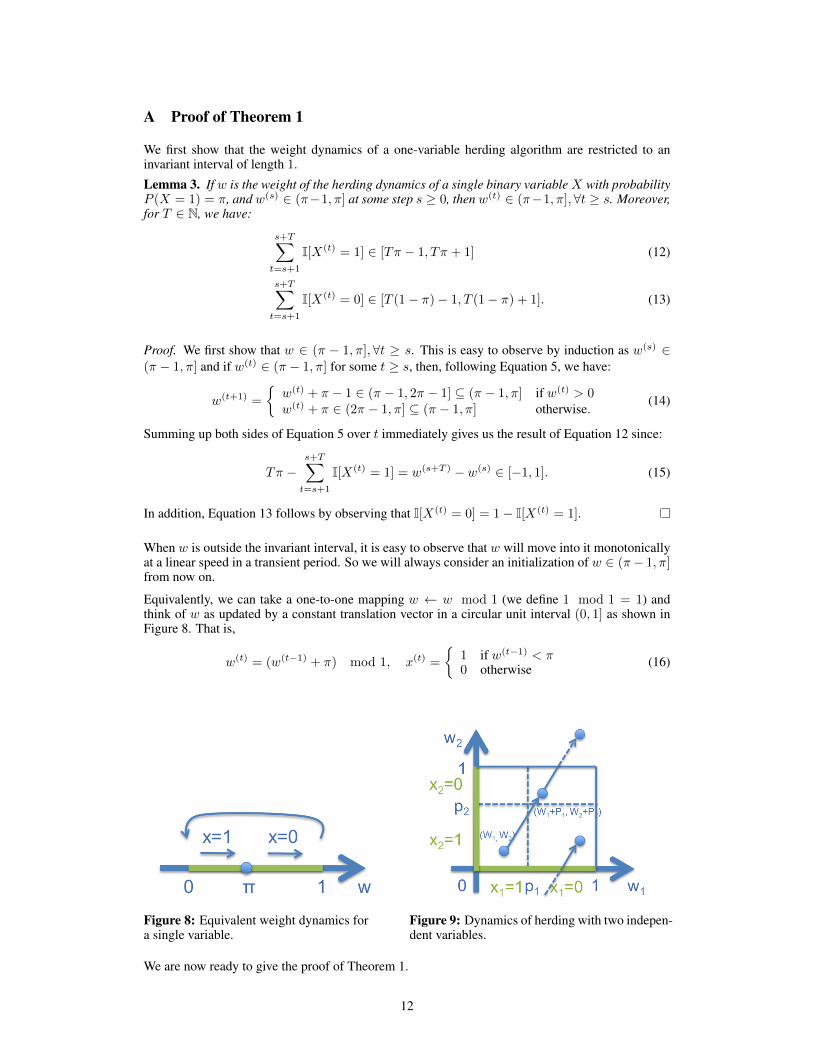
We begin the theoretical analysis with a graph of one binary variable. For this graph, there is onlyone weight w. Denote π(X = 1) as π for notational simplicity. The sequence of X is determinedby the dynamics of w (shown in Figure 1):

w(t) = w(t−1) + π − I(w(t−1) > 0), X(t) =

{1 if w(t−1) > 00 otherwise (5)

Lemma 3 in the appendix shows that (π − 1, π] is the invariant interval of the dynamics, and thestate X = 1 is visited at a frequency close to π with an error:

|P (τ)T (X = 1)− π| ≤ 1

T(6)

This is known as the fast moment matching property in [24, 23, 10]. We will show in the next twotheorems that the fast moment matching property also holds for two special types of graphs, withproofs provided in the appendix.

Figure 1: Herding dynamics for a single variable.

In an empty graph, all the variables are independent of each other and herded Gibbs reduces torunning N one-variable chains in parallel. Denote the marginal distribution πi := π(Xi = 1).

Examples of failing convergence in the presence of rational ratios between the πis were observed in[4]. There the need for further theoretical research on this matter was pointed out. The followingtheorem provides formal conditions for convergence in the restricted domain of empty graphs.Theorem 1. For an empty graph, when herded Gibbs has a fixed scanning order, and{1, π1, . . . , πN} are rationally independent, the empirical distribution P (τ)

T converges to the tar-get distribution π as T →∞ for any τ ≥ 0.

A set of n real numbers, x1, x2, . . . , xn, is said to be rationally independent if for any set of rationalnumbers, a1, a2, . . . , an, we have

∑ni=1 aixi = 0⇔ ai = 0,∀1 ≤ i ≤ n. The proof of Theorem 1

consists of first formulating the dynamics of the weight vector as a constant translation mapping ina circular unit cube, and then proving that the weights are uniformly distributed by making use ofKronecker-Weyl’s theorem [25].

For fully-connected (complete) graphs, convergence is guaranteed even with rational ratios. In fact,herded Gibbs converges to the target joint distribution at a rate of O(1/T ) with a O(log(T )) burn-inperiod. This statement is formalized in Theorem 2.Theorem 2. For a fully-connected graph, when herded Gibbs has a fixed scanning order and aDobrushin coefficient of the corresponding Gibbs sampler η < 1, there exist constants l > 0, andB > 0 such that

dv(P(τ)T − π) ≤ λ

T,∀T ≥ T ∗, τ > τ∗(T ) (7)

where λ = 2N(1+η)l(1−η) , T ∗ = 2B

l , τ∗(T ) = log 21+η

((1−η)lT

4N

), and dv(δπ) := 1

2 ||δπ||1.

The constants l and B are defined in Equation 31 for Proposition 4 in the appendix. If we ignore theburn-in period and start collecting samples simply from the beginning, we achieve a convergence rateof O( log(T )

T ) as stated in Corollary 10 in the appendix. The constant l in the convergence rate has anexponential term, with N in the exponent. An exponentially large constant seems to be unavoidablefor any sampling algorithm when considering the convergence to a joint distribution with 2N states.As for the marginal distributions, it is obvious that the convergence rate of herded Gibbs is also

4

O(1/T ) because marginal probabilities are linear functions of the joint distribution. However, inpractice, we observe very rapid convergence results for the marginals, so stronger theoretical resultsabout the convergence of the marginal distributions seem plausible.

The proof proceeds by first bounding the discrepancy between the chain of empirical estimates ofthe joint obtained by averaging over T herded Gibbs samples, {P (s)

T }, s ≥ τ , and a Gibbs chaininitialized at P (τ)

T . After one iteration, this discrepancy is bounded above by O(1/T ).

The Gibbs chain has geometric convergence to π and the distance between the Gibbs and herdedGibbs chains is bounded by O(1/T ). The geometric convergence rate to π dominates the discrep-ancy of herded Gibbs and thus we infer that P (τ)

T converges to π geometrically. To round-off theproof, we must find a limiting value for τ . The proof concludes with an O(log(T )) burn-in for τ .

However, for a generic graph we have no mathematical guarantees on the convergence rate of herdedGibbs. In fact, one can easily construct synthetic examples for which herded Gibbs does not seemto converge to the true marginals and joint distribution. For the examples covered by our theoremsand for examples with real data, herded Gibbs demonstrates good behaviour. The exact conditionsunder which herded Gibbs converges for sparsely connected graphs are still unknown.

4 Experiments

4.1 Simple Complete Graph

We begin with an illustration of how herded Gibbs substantially outperforms Gibbs on a simplecomplete graph. In particular, we consider a fully-connected model of two variables, X1 and X2,as shown in Figure 2; the joint distribution of these variables is shown in Table 1. Figure 3 showsthe marginal distribution P (X1 = 1) approximated by both Gibbs and herded Gibbs for differentε. As ε decreases, both approaches require more iterations to converge, but herded Gibbs clearlyoutperforms Gibbs. The figure also shows that Herding does indeed exhibit a linear convergencerate.

X1 X2

Figure 2: Two-variable model.

X1 = 0 X1 = 1 P(X2)X2 = 0 1/4− ε ε 1/4X2 = 1 ε 3/4− ε 3/4P(X1) 1/4 3/4 1

Table 1: Joint distribution of the two-variable model.

4.2 MRF for Image Denoising

Next, we consider the standard setting of a grid-lattice MRF for image denoising. Let us assumethat we have a binary image corrupted by noise, and that we want to infer the original clean image.Let Xi ∈ {−1,+1} denote the unknown true value of pixel i, and yi the observed, noise-corruptedvalue of this pixel. We take advantage of the fact that neighboring pixels are likely to have the samelabel by defining an MRF with an Ising prior. That is, we specify a rectangular 2D lattice with thefollowing pair-wise clique potentials:

ψij(xi, xj) =

(eJij e−Jij

e−Jij eJij

)(8)

and joint distribution:

p(x|J) = 1

Z(J)

∏i∼j

ψij(xi, xj) =1

Z(J)exp

1

2

∑i∼j

Jijxixj

, (9)

where i ∼ j is used to indicate that nodes i and j are connected. The known parameters Jij establishthe coupling strength between nodes i and j. Note that the matrix J is symmetric. If all the Jij > 0,then neighboring pixels are likely to be in the same state.

5

(a) Approximate marginals obtained via Gibbs (blue) and herded Gibbs (red).

(b) Log-log plot of marginal approximation errors obtained via Gibbs (blue) and herded Gibbs (red).

(c) Inverse of marginal approximation errors obtained via Gibbs (blue) and herded Gibbs (red).

Figure 3: (a) Approximating a marginal distribution with Gibbs (blue) and herded Gibbs (red) for anMRF of two variables, constructed so as to make the move from state (0, 0) to (1, 1) progressivelymore difficult as ε decreases. The four columns, from left to right, are for ε = 0.1, ε = 0.01,ε = 0.001 and ε = 0.0001. Table 1 provides the joint distribution for these variables. The errorbars for Gibbs correspond to one standard deviation. Rows (b) and (c) illustrate that the empiricalconvergence rate of herded Gibbs matches the expected theoretical rate. In the plots of rows (b)and (c), the upper-bound in the error of herded Gibbs was used to remove the oscillations so as toillustrate the behaviour of the algorithm more clearly.

The MRF model combines the Ising prior with a likelihood model as follows:

p(x,y) = p(x)p(y|x) =

1

Z

∏i∼j

ψij(xi, xj)

.[∏i

p(yi|xi)

](10)

The potentials ψij encourage label smoothness. The likelihood terms p(yi|xi) are conditionallyindependent (e.g. Gaussians with known variance σ2 and mean µ centered at each value of xi,denoted µxi ). In more precise terms,

p(x,y|J,µ, σ) = 1

Z(J,µ, σ)exp

1

2

∑i∼j

Jijxixj −1

2σ2

∑i

(yi − µxi)2 . (11)

6

Figure 4: Original image (left) and its corrupted version (right), with noise parameter σ = 4.

Figure 5: Reconstruction errors for the image denoising task. The results are averaged across10 corrupted images with Gaussian noise N (0, 16). The error bars correspond to one standarddeviation. Mean field requires the specification of the damping factor D.

When the coupling parameters Jij are identical, say Jij = J , we have∑ij Jijf(xi, xj) =

J∑ij f(xi, xj). Hence, different neighbor configurations result in the same value of

J∑ij f(xi, xj). If we store the conditionals for configurations with the same sum together, we

only need to store as many conditionals as different possible values that the sum could take. Thisenables us to develop a shared version of herded Gibbs that is more memory efficient where we onlymaintain and update weights for distinct states of the Markov blanket of each variable.

In this exemplary image denoising experiment, noisy versions of the binary image, seen in Figure 4(left), were created through the addition of Gaussian noise, with varying σ. Figure 4 (right) shows acorrupted image with σ = 4. The L2 reconstruction errors as a function of the number of iterations,for this example, are shown in Figure 5. The plot compares the herded Gibbs method against Gibbsand two versions of mean field with different damping factors [19]. The results demonstrate that theherded Gibbs techiques are among the best methods for solving this task.

A comparison for different values σ is presented in Table 2. As expected mean field does well in thelow-noise scenario, but the performance of the shared version of herded Gibbs as the noise increasesis significantly better.

7

Table 2: Errors of image denoising example after 30 iterations (all measurements have been scaledby ×10−3). We use an Ising prior with Jij = 1 and four Gaussian noise models with differentσ’s. For each σ, we generated 10 corrupted images by adding Gaussian noise. The final resultsshown here are averages and standard deviations (in parentheses) across the 10 corrupted images. Ddenotes the damping factor in mean field.

PPPPPPMethodσ 2 4 6 8

Herded Gibbs 21.58(0.26) 32.07(0.98) 47.52(1.64) 67.93(2.78)Herded Gibbs - shared 22.24(0.29) 31.40(0.59) 42.62(1.98) 58.49(2.86)Gibbs 21.63(0.28) 37.20(1.23) 63.78(2.41) 90.27(3.48)Mean field (D=0.5) 15.52(0.30) 41.76(0.71) 76.24(1.65) 104.08(1.93)Mean field (D=1) 17.67(0.40) 32.04(0.76) 51.19(1.44) 74.74(2.21)

Other

’

Person

Zed

Other

s

Other

.

Other

’

Person

Zed

Other

s

Other

dead

Other

.

Other

dead

Other

baby

Figure 6: Typical skip-chain CRF model for named entity recognition.

4.3 CRF for Named Entity Recognition

Named Entity Recognition (NER) involves the identification of entities, such as people and loca-tions, within a text sample. A conditional random fied (CRF) for NER models the relationshipbetween entity labels and sentences with a conditional probability distribution: P (Y |X, θ), whereX is a sentence, Y is a labeling, and θ is a vector of coupling parameters. The parameters, θ, are fea-ture weights and model relationships between variables Yi and Xj or Yi and Yj . A chain CRF onlyemploys relationships between adjacent variables, whereas a skip-chain CRF can employ relation-ships between variables where subscripts i and j differ dramatically. Skip-chain CRFs are importantin language tasks, such as NER and semantic role labeling, because they allow us to model longdependencies in a stream of words, see Figure 6.

Once the parameters have been learned, the CRF can be used for inference; a labeling for somesentence X is found by maximizing the above probability. Inference for CRF models in the NERdomain is typically carried out with the Viterbi algorithm. However, if we want to accommodate longterm dependencies, thus resulting in the so called skip-chain CRFs, Viterbi becomes prohibitivelyexpensive. To surmount this problem, the Stanford named entity recognizer [15] makes use ofannealed Gibbs sampling.

To demonstrate herded Gibbs on a practical application of great interest in text mining, we modifythe standard inference procedure of the Stanford named entity recognizer by replacing the annealedGibbs sampler with the herded Gibbs sampler. The herded Gibbs sampler in not annealed. To findthe maximum a posteriori sequence Y , we simply choose the sample with highest joint discreteprobability. In order to be able to compare against Viterbi, we have purposely chosen to use single-chain CRFs. We remind the reader, however, that the herded Gibbs algorithm could be used in caseswhere Viterbi inference is not possible.

We used the pre-trained 3-class CRF model in the Stanford NER package [15]. This model is alinear chain CRF with pre-defined features and pre-trained feature weights, θ. For the test set, weused the corpus for the NIST 1999 IE-ER Evaluation. Performance is measured in per-entity F1(F1 = 2 · precision·recall

precision+recall

). For all the methods, except Viterbi, we show F1 scores after 100, 400 and

800 iterations in Table 3. For Gibbs, the results shown are the averages and standard deviationsover 5 random runs. We used a linear annealing schedule for Gibbs. As the results illustrate,

8

”Pumpkin” (Tim Roth) and ”Honey Bunny” (Amanda Plummer) are having breakfast in adiner. They decide to rob it after realizing they could make money off the customers aswell as the business, as they did during their previous heist. Moments after they initiatethe hold-up, the scene breaks off and the title credits roll. As Jules Winnfield (Samuel L.Jackson) drives, Vincent Vega (John Travolta) talks about his experiences in Europe, fromwhere he has just returned: the hash bars in Amsterdam, the French McDonald’s and its”Royale with Cheese”.

Figure 7: Results for the application of the NER CRF to a random Wikipedia sample [1]. Entitiesare automatically classified as Person, Location and Organization.

herded Gibbs attains the same accuracy as Viterbi and it is faster than annealed Gibbs. UnlikeViterbi, herded Gibbs can be easily applied to skip-chain CRFs. After only 400 iterations (90.5seconds), herded Gibbs already achieves an F1 score of 84.75, while Gibbs, even after 800 iterations(115.9 seconds) only achieves an F1 score of 84.61. The experiment thus clearly demonstrates that(i) herded Gibbs does no worse than the optimal solution, Viterbi, and (ii) herded Gibbs yieldsmore accurate results for the same amount of computation. Figure 7 provides a representative NERexample of the performance of Gibbs, herded Gibbs and Viterbi (all methods produced the sameannotation for this short example).

Table 3: Gibbs, herded Gibbs and Viterbi for the NER task. The average computational time eachapproach took to do inference for the entire test set is listed (in square brackets). After only 400iterations (90.48 seconds), herded Gibbs already achieves an F1 score of 84.75, while Gibbs, evenafter 800 iterations (115.92 seconds) only achieves an F1 score of 84.61. For the same computation,herded Gibbs is more accurate than Gibbs.

``````````MethodIterations 100 400 800

Annealed Gibbs 84.36(0.16) [55.73s] 84.51(0.10) [83.49s] 84.61(0.05) [115.92s]Herded Gibbs 84.70 [59.08s] 84.75 [90.48s] 84.81 [132.00s]Viterbi 84.81[46.74s]

5 Conclusions and Future Work

In this paper, we introduced herded Gibbs, a deterministic variant of the popular Gibbs sampling al-gorithm. While Gibbs relies on drawing samples from the full-conditionals at random, herded Gibbsgenerates the samples by matching the full-conditionals. Importantly, the herded Gibbs algorithm isvery close to the Gibbs algorithm and hence retains its simplicity of implementation.

The synthetic, denoising and named entity recognition experiments provided evidence that herdedGibbs outperforms Gibbs sampling. However, as discussed, herded Gibbs requires storage of theconditional distributions for all instantiations of the neighbors in the worst case. This storage re-quirement indicates that it is more suitable for sparse probabilistic graphical models, such as theCRFs used in information extraction. At the other extreme, the paper advanced the theory of de-terministic sampling by showing that herded Gibbs converges with rate O(1/T ) for models withindependent variables and fully-connected models. Thus, there is gap between theory and practicethat needs to be narrowed. We do not anticipate that this will be an easy task, but it is certainly a keydirection for future work.

We should mention that it is also possible to design parallel versions of herded Gibbs in a Jacobifashion. We have indeed studied this and found that these are less efficient than the Gauss-Seidelversion of herded Gibbs discussed in this paper. However, if many cores are available, we stronglyrecommend the Jacobi (asynchronous) implementation as it will likely outperform the Gauss-Seidel(synchronous) implementation.

9

The design of efficient herding algorithms for densely connected probabilistic graphical modelsremains an important area for future research. Such algorithms, in conjunction with Rao Black-wellization, would enable us to attack many statistical inference tasks, including Bayesian variableselection and Dirichlet processes.

There are also interesting connections with other algorithms to explore. If, for a fully connectedgraphical model, we build a new graph where every state is a node and directed connections existbetween nodes that can be reached with a single herded Gibbs update, then herded Gibbs becomesequivalent to the Rotor-Router model of Alex Holroyd and Jim Propp1 [13]. This deterministic ana-logue of a random walk has provably superior concentration rates for quantities such as normalizedhitting frequencies, hitting times and occupation frequencies. In line with our own convergenceresults, it is shown that discrepancies in these quantities decrease as O(1/T ) instead of the usualO(1/

√T ). We expect that many of the results from this literature apply to herded Gibbs as well.

The connection with the work of Art Owen and colleagues, see for example [7], also needs tobe explored further. Their work uses completely uniformly distributed (CUD) sequences to driveMarkov chain Monte Carlo schemes. It is not clear, following discussions with Art Owen, that CUDsequences can be constructed in a greedy way as in herding.

References

[1] Pulp fiction - wikipedia, the free encyclopedia @ONLINE, June 2012.

[2] D. H. Ackley, G. Hinton, and T.. Sejnowski. A learning algorithm for Boltzmann machines.Cognitive Science, 9:147–169, 1985.

[3] C. Andrieu, N. de Freitas, A. Doucet, and M. I. Jordan. An Introduction to MCMC for MachineLearning. Machine Learning, 50(1):5–43, 2003.

[4] F. Bach, S. Lacoste-Julien, and G. Obozinski. On the equivalence between herding and condi-tional gradient algorithms. In International Conference on Machine Learning, 2012.

[5] P. Bremaud. Markov chains: Gibbs fields, Monte Carlo simulation, and queues, volume 31.Springer, 1999.

[6] P. Carbonetto, J. Kisynski, N. de Freitas, and D. Poole. Nonparametric Bayesian logic. InUncertainty in Artificial Intelligence, pages 85–93, 2005.

[7] S. Chen, J. Dick, and A. B. Owen. Consistency of Markov chain quasi-Monte Carlo on con-tinuous state spaces. Annals of Statistics, 39(2):673–701, 2011.

[8] Y. Chen, M. Welling, and A.J. Smola. Supersamples from kernel-herding. In Uncertainty inArtificial Intelligence, pages 109–116, 2010.

[9] A. Doucet, N. de Freitas, and N. Gordon. Sequential Monte Carlo Methods in Practice. Statis-tics for Engineering and Information Science. Springer, 2001.

[10] A. Gelfand, Y. Chen, L. van der Maaten, and M. Welling. On herding and the perceptroncycling theorem. In Advances in Neural Information Processing Systems, pages 694–702,2010.

[11] N. D. Goodman, V. K. Mansinghka, D. M. Roy, K. Bonawitz, and J. B. Tenenbaum. Church:a language for generative models. Uncertainty in Artificial Intelligence, 2008.

[12] G.E. Hinton and R.R. Salakhutdinov. Reducing the dimensionality of data with neural net-works. Science, 313(5786):504–507, 2006.

[13] Alexander E Holroyd and James Propp. Rotor walks and Markov chains. Algorithmic Proba-bility and Combinatorics, 520:105–126, 2010.

[14] F. Huszar and D. Duvenaud. Optimally-weighted herding is Bayesian quadrature. Arxivpreprint arXiv:1204.1664, 2012.

[15] T. Grenager J. R. Finkel and C. Manning. Incorporating non-local information into informa-tion extraction systems by Gibbs sampling. In Proceedings of the 43rd Annual Meeting onAssociation for Computational Linguistics, ACL ’05, pages 363–370, Stroudsburg, PA, USA,2005. Association for Computational Linguistics.

1We thank Art Owen for pointing out this connection.

10

[16] J. S. Liu. Monte Carlo strategies in scientific computing. Springer, 2001.[17] D. J. Lunn, A. Thomas, N. Best, and D. Spiegelhalter. WinBUGS a Bayesian modelling frame-

work: Concepts, structure, and extensibility. Statistics and Computing, 10(4):325–337, 2000.[18] B. Milch and S. Russell. General-purpose MCMC inference over relational structures. In

Uncertainty in Artificial Intelligence, pages 349–358, 2006.[19] K. P. Murphy. Machine Learning: a Probabilistic Perspective. MIT Press, 2012.[20] I. Murray and L. T. Elliott. Driving Markov chain Monte Carlo with a dependent random

stream. Technical Report arXiv:1204.3187, 2012.[21] I. Porteous, D. Newman, A. Ihler, A. Asuncion, P. Smyth, and M. Welling. Fast collapsed

Gibbs sampling for latent Dirichlet allocation. In ACM SIGKDD international conference onKnowledge discovery and data mining, pages 569–577, 2008.

[22] C. P. Robert and G. Casella. Monte Carlo Statistical Methods. Springer, 2nd edition, 2004.[23] M. Welling. Herding dynamic weights for partially observed random field models. In Uncer-

tainty in Artificial Intelligence, pages 599–606, 2009.[24] M. Welling. Herding dynamical weights to learn. In International Conference on Machine

Learning, pages 1121–1128, 2009.[25] Hermann Weyl. Uber die gleichverteilung von zahlen mod. eins. Mathematische Annalen,

77:313–352, 1916.

11

A Proof of Theorem 1

We first show that the weight dynamics of a one-variable herding algorithm are restricted to aninvariant interval of length 1.

Lemma 3. If w is the weight of the herding dynamics of a single binary variable X with probabilityP (X = 1) = π, and w(s) ∈ (π−1, π] at some step s ≥ 0, then w(t) ∈ (π−1, π],∀t ≥ s. Moreover,for T ∈ N, we have:

s+T∑t=s+1

I[X(t) = 1] ∈ [Tπ − 1, Tπ + 1] (12)

s+T∑t=s+1

I[X(t) = 0] ∈ [T (1− π)− 1, T (1− π) + 1]. (13)

Proof. We first show that w ∈ (π − 1, π],∀t ≥ s. This is easy to observe by induction as w(s) ∈(π − 1, π] and if w(t) ∈ (π − 1, π] for some t ≥ s, then, following Equation 5, we have:

w(t+1) =

{w(t) + π − 1 ∈ (π − 1, 2π − 1] ⊆ (π − 1, π] if w(t) > 0w(t) + π ∈ (2π − 1, π] ⊆ (π − 1, π] otherwise.

(14)

Summing up both sides of Equation 5 over t immediately gives us the result of Equation 12 since:

Tπ −s+T∑t=s+1

I[X(t) = 1] = w(s+T ) − w(s) ∈ [−1, 1]. (15)

In addition, Equation 13 follows by observing that I[X(t) = 0] = 1− I[X(t) = 1].

When w is outside the invariant interval, it is easy to observe that w will move into it monotonicallyat a linear speed in a transient period. So we will always consider an initialization of w ∈ (π− 1, π]from now on.

Equivalently, we can take a one-to-one mapping w ← w mod 1 (we define 1 mod 1 = 1) andthink of w as updated by a constant translation vector in a circular unit interval (0, 1] as shown inFigure 8. That is,

w(t) = (w(t−1) + π) mod 1, x(t) =

{1 if w(t−1) < π0 otherwise (16)

Figure 8: Equivalent weight dynamics fora single variable.

Figure 9: Dynamics of herding with two indepen-dent variables.

We are now ready to give the proof of Theorem 1.

12

Proof of Theorem 1. For an empty graph of N independent vertices, the dynamics of the weightvector w are equivalent to a constant translation mapping in an N -dimensional circular unit space(0, 1], as shown in Figure 9:

w(t) = (w(t−1) + π) mod 1

= (w(0) + tπ) mod 1, x(t)i =

{1 if w(t−1)

i < πi0 otherwise

,∀1 ≤ i ≤ N (17)

The Kronecker-Weyl theorem [25] states that the sequence w(t) = tπ mod 1, t ∈ Z+ is equidis-tributed (or uniformly distributed) on (0, 1] if and only if (1, π1, . . . , πN ) is rationally indepen-dent. Since we can define a one-to-one volume preserving transformation between w(t) and w(t)

as (w(t) + w(0)) mod 1 = w(t), the sequence of weights {w(t)} is also uniformly distributed in(0, 1]N .

Define the mapping from a state value xi to an interval of wi as

Ai(x) =

{(0, πi] if x = 1(πi, 1] if x = 0

(18)

and let |Ai| be its measure. We obtain the limiting distribution of the joint state as

limT→∞

P(τ)T (X = x) = lim

T→∞

1

T

T∑t=1

I

[w(t−1) ∈

N∏i=1

Ai(xi)

]

=

N∏i=1

|Ai(xi)|

=

N∏i=1

π(Xi = xi)

= π(X = x) (19)

13

B Proof of Theorem 2

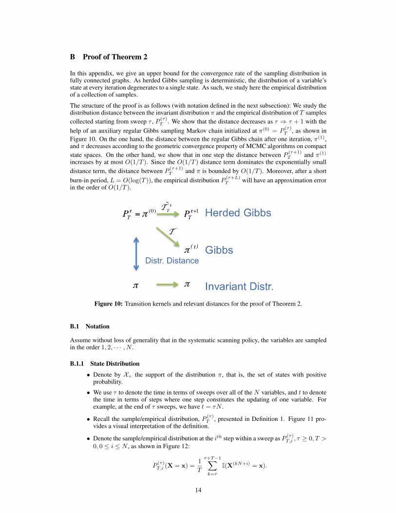
In this appendix, we give an upper bound for the convergence rate of the sampling distribution infully connected graphs. As herded Gibbs sampling is deterministic, the distribution of a variable’sstate at every iteration degenerates to a single state. As such, we study here the empirical distributionof a collection of samples.

The structure of the proof is as follows (with notation defined in the next subsection): We study thedistribution distance between the invariant distribution π and the empirical distribution of T samplescollected starting from sweep τ , P (τ)

T . We show that the distance decreases as τ ⇒ τ + 1 with thehelp of an auxiliary regular Gibbs sampling Markov chain initialized at π(0) = P

(τ)T , as shown in

Figure 10. On the one hand, the distance between the regular Gibbs chain after one iteration, π(1),and π decreases according to the geometric convergence property of MCMC algorithms on compactstate spaces. On the other hand, we show that in one step the distance between P (τ+1)

T and π(1)

increases by at most O(1/T ). Since the O(1/T ) distance term dominates the exponentially smalldistance term, the distance between P (τ+1)

T and π is bounded by O(1/T ). Moreover, after a shortburn-in period, L = O(log(T )), the empirical distribution P (τ+L)

T will have an approximation errorin the order of O(1/T ).

Figure 10: Transition kernels and relevant distances for the proof of Theorem 2.

B.1 Notation

Assume without loss of generality that in the systematic scanning policy, the variables are sampledin the order 1, 2, · · · , N .

B.1.1 State Distribution

• Denote by X+ the support of the distribution π, that is, the set of states with positiveprobability.

• We use τ to denote the time in terms of sweeps over all of the N variables, and t to denotethe time in terms of steps where one step constitutes the updating of one variable. Forexample, at the end of τ sweeps, we have t = τN .

• Recall the sample/empirical distribution, P (τ)T , presented in Definition 1. Figure 11 pro-

vides a visual interpretation of the definition.

• Denote the sample/empirical distribution at the ith step within a sweep as P (τ)T,i , τ ≥ 0, T >

0, 0 ≤ i ≤ N , as shown in Figure 12:

P(τ)T,i (X = x) =

1

T

τ+T−1∑k=τ

I(X(kN+i) = x).

14

Figure 11: Distribution over time at the end of every sweep.

This is the distribution of T samples collected at the ith step of every sweep, starting fromthe τ th sweep. Clearly, P (τ)

T = P(τ)T,0 = P

(τ−1)T,N .

Figure 12: Distribution over time within a sweep.

• Denote the distribution of a regular Gibbs sampling Markov chain afterL sweeps of updatesover the N variables with π(L), L ≥ 0.

For a given time τ , we construct a Gibbs Markov chain with initial distribution π0 = P(τ)T

and the same scanning order of herded Gibbs, as shown in Figure 10.

B.1.2 Transition Kernel

• Denote the transition kernel of regular Gibbs for the step of updating a variable Xi with Ti,and for a whole sweep with T .By definition, π0T = π1. The transition kernel for a single step can be represented as a2N × 2N matrix:

Ti(x,y) ={

0 if x−i 6= y−iπ(Xi = yi|x−i) otherwise , 1 ≤ i ≤ N,x,y ∈ {0, 1}N (20)

where x is the current state vector of N variables, y is the state of the next step, and x−idenotes all the components of x excluding the ith component. If π(x−i) = 0, the condi-tional probability is undefined and we set it with an arbitrary distribution. Consequently, Tcan also be represented as:

T = T1T2 · · · TN .• Denote the Dobrushin ergodic coefficient [5] of the regular Gibbs kernel with η ∈ [0, 1].

When η < 1, the regular Gibbs sampler has a geometric rate of convergence of

dv(π(1) − π) = dv(T π(0) − π) ≤ ηdv(π(0) − π),∀π(0). (21)

A common sufficient condition for η < 1 is that π(X) is strictly positive.

• Consider the sequence of sample distributions P (τ)T , τ = 0, 1, · · · in Figures 11 and 12. We

define the transition kernel of herded Gibbs for the step of updating variable Xi with T (τ)T,i ,

and for a whole sweep with T (τ)T .

Unlike regular Gibbs, the transition kernel is not homogeneous. It depends on both thetime τ and the sample size T . Nevertheless, we can still represent the single step transition

15

kernel as a matrix:

T (τ)T,i (x,y) =

{0 if x−i 6= y−i

P(τ)T,i (Xi = yi|x−i) if x−i = y−i

, 1 ≤ i ≤ N,x,y ∈ {0, 1}N ,

(22)where P (τ)

T,i (Xi = yi|x−i) is defined as:

P(τ)T,i (Xi = yi|x−i) =

Nnum

Nden

Nnum = TP(τ)T,i (X−i = x−i, Xi = yi) =

τ+T−1∑k=τ

I(X(kN+i)−i = x−i, X

(kN+i)i = yi)

Nden = TP(τ)T,i−1(X−i = x−i) =

τ+T−1∑k=τ

I(X(kN+i−1)−i = x−i), (23)

where Nnum is the number of occurrences of a joint state, and Nden is the number of oc-currences of a conditioning state in the previous step. When π(x−i) = 0, we know thatNden = 0 with a proper initialization of herded Gibbs, and we simply set T (τ)

T,i = Ti forthese entries. It is not hard to verify the following identity by expanding every term withits definition

P(τ)T,i = P

(τ)T,i−1T

(τ)T,i

and consequently,P

(τ+1)T = P

(τ)T T

(τ)T

withT (τ)T = T (τ)

T,1 T(τ)T,2 · · · T

(τ)T,N .

B.2 Linear Visiting Rate

We prove in this section that every joint state in the support of the target distribution is visited, atleast, at a linear rate. This result will be used to measure the distance between the Gibbs and herdedGibbs transition kernels.Proposition 4. If a graph is fully connected, herded Gibbs sampling scans variables in a fixed order,and the corresponding Gibbs sampling Markov chain is irreducible, then for any state x ∈ X+ andany index i ∈ [1, N ], the state is visited at least at a linear rate. Specifically,

∃l > 0, B > 0, s.t.,∀i ∈ [1, N ],x ∈ X+, T ∈ N, s ∈ Ns+T−1∑k=s

I[X(t=Nk+i) = x

]≥ lT −B (24)

Denote the minimum nonzero conditional probability as

πmin = min1≤i≤N,π(xi|x−i)>0

π(xi|x−i).

The following lemma, which is needed to prove Proposition 4, gives an inequality between thenumber of visits of two sets of states in consecutive steps.Lemma 5. For any integer i ∈ [1, N ] and two sets of states X,Y ⊆ X+ with a mapping F : X→ Ythat satisfies the following condition:

∀x ∈ X,F(x)−i = x−i, ∪x∈XF (x) = Y, (25)

we have that, for any s ≥ 0 and T > 0, the number of times Y is visited in the set of stepsCi = {t = kN + i : s ≤ k ≤ k + T − 1} is lower bounded by a function of the number of times Xis visited in the previous steps Ci−1 = {t = kN + i− 1 : s ≤ k ≤ k + T − 1} as:∑

t∈Ci

I[X(t) ∈ Y

]≥ πmin

∑t∈Ci−1

I[X(t) ∈ X

]− |Y| (26)

16

Proof. As a complement to Condition 25, we can define F−1 as the inverse mapping from Y tosubsets of X so that for any y ∈ Y, x ∈ F−1(y), we have x−i = y−i, and ∪y∈YF−1(y) = X.

Consider any state y ∈ Y, when y is visited in Ci, the weight wi,y−i is active. Let us denotethe set of all the steps in [sN + 1, s(N + T ) + N ] when wi,y−i is active by Ci(y−i), that is,Ci(y−i) = {t : t ∈ Ci,X(t)

−i = y−i}. Applying Lemma 3 we get

∑t∈Ci

I[X(t) = y

]≥ π(yi|y−i)|Ci(y−i)| − 1 ≥ πmin|Ci(y−i)| − 1. (27)

Since the variables X−i are not changed at steps in Ci, we have

|Ci(y−i)| =∑

t∈Ci−1

I[X

(t)−i = y−i

]≥

∑t∈Ci−1

I[X(t) ∈ F−1(y)

]. (28)

Combining the fact that ∪y∈YF−1(y) = X and summing up both sides of Equation 27 over Yproves the lemma:

∑t∈Ci

I[X(t) ∈ Y

]≥∑y∈Y

πmin

∑t∈Ci−1

I[X(t) ∈ F−1(y)

]− 1

≥ πmin

∑t∈Ci−1

I[X(t) ∈ X

]−|Y|.

(29)

Remark 6. A fully connected graph is a necessary condition for the application of Lemma 3 in theproof. If a graph is not fully connected (N(i) 6= −i), a weight wi,yN(i)

may be shared by multiplefull conditioning states. In this case Ci(y−i) is no longer a consecutive sequence of times when theweight is updated, and Lemma 3 does not apply here.

Now let us prove Proposition 4 by iteratively applying Lemma 5.

Proof of Proposition 4. Because the corresponding Gibbs sampler is irreducible and any Gibbs sam-pler is aperiodic, there exists a constant t∗ > 0 such that for any state y ∈ X+, and any step in asweep, i, we can find a path of length t∗ for any state x ∈ X+ with a positive transition probability,Path(x) = (x = x(0),x(1), . . . ,x(t∗) = y), to connect from x to y, where each step of the pathfollows the Gibbs updating scheme. For a strictly positive distribution, the minimum value of t∗ isN .

Denote τ∗ = dt∗/Ne and the jth element of the path Path(x) as Path(x, j). We can define t∗ +1subsets Sj ⊆ X+, 0 ≤ j ≤ t∗ as the union of all the jth states in the path from any state in X+:

Sj = ∪x∈X+Path(x, j)

By definition of these paths, we know S0 = X+ and St∗ = {y}, and there exits an integer i(j) and amapping Fj : Sj−1 → Sj ,∀j that satisfy the condition in Lemma 5 (i(j) is the index of the variableto be updated, and the mapping is defined by the transition path). Also notice that any state in Sjcan be different from y by at most min{N, t∗ − j} variables, and therefore |Sj | ≤ 2min{N,t∗−j}.

17

Let us apply Lemma 5 recursively from j = t∗ to 1 as

s+T−1∑k=s

I[X(t=Nk+i) = y

]≥

s+T−1∑k=s+τ∗

I[X(t=Nk+i) = y

]

=

s+T−1∑k=s+τ∗

I[X(t=Nk+i) ∈ St∗

]

≥ πmin

s+T−1∑k=s+τ∗

I[X(t=Nk+i−1) ∈ St∗−1

]− |St∗ |

≥ · · ·

≥ πt∗

min

s+T−1∑k=s+τ∗

I[X(t=Nk+i−t∗) ∈ S0 = X+

]−t∗−1∑j=0

πjmin|St∗−j |

≥ πt∗

min(T − τ∗)−t∗−1∑j=0

πjmin2min{N,j}. (30)

The proof is concluded by choosing the constants

l = πt∗

min, B = τ∗πt∗

min +

t∗−1∑j=0

πjmin2min{N,j}. (31)

B.3 Herded Gibbs’s Transition Kernel T (τ)T is an Approximation to T

The following proposition shows that T (τ)T is an approximation to the regular Gibbs sampler’s tran-

sition kernel T with an error of O(1/T ).

Proposition 7. For a fully connected graph, if the herded Gibbs has a fixed scanning order and thecorresponding Gibbs sampling Markov chain is irreducible, then for any τ ≥ 0, T ≥ T ∗ := 2B

lwhere l and B are the constants in Proposition 4, the following inequality holds:

‖T (τ)T − T ‖∞ ≤

4N

lT(32)

Proof. When x 6∈ X+, we have the equality T (τ)T,i (x,y) = Ti(x,y) by definition. When x ∈ X+

but y 6∈ X+, then Nden = 0 (see the notation of T (τ)T for definition of Nden) as y will never be

visited and thus T (τ)T,i (x,y) = 0 = Ti(x,y) also holds. Let us consider the entries in T (τ)

T,i (x,y)with x,y ∈ X+ in the following.

Because X−i is not updated at ith step of every sweep, we can replace i−1 in the definition of Ndenby i and get

Nden =

τ+T−1∑k=τ

I(X(kN+i)−i = x−i).

Notice that the set of times {t = kN+i : τ ≤ k ≤ τ+T −1,Xt−i = x−i)}, whose size isNden, is a

consecutive set of times when wi,x−i is updated. By Lemma 3, we obtain a bound for the numerator

Nnum ∈ [Ndenπ(Xi = yi|x−i)− 1, Ndenπ(Xi = yi|x−i) + 1]⇔

|P (τ)T,i (Xi = yi|x−i)− π(Xi = yi|x−i)| = |

Nnum

Nden− π(Xi = yi|x−i)| ≤

1

Nden. (33)

Also by Proposition 4, we know every state in X+ is visited at a linear rate, there hence existconstants l > 0 and B > 0, such that the number of occurrence of any conditioning state x−i, Nden,

18

is bounded by

Nden ≥τ+T−1∑k=τ

I(X(kN+i) = x) ≥ lT −B ≥ l

2T, ∀T ≥ 2B

l. (34)

Combining equations (33) and (34), we obtain

|P (τ)T,i (Xi = yi|x−i)− π(Xi = yi|x−i)| ≤

2

lT, ∀T ≥ 2B

l. (35)

Since the matrix T (τ)T,i and Ti differ only at those elements where x−i = y−i, we can bound the L1

induced norm of the transposed matrix of their difference by

‖(T (τ)T,i − Ti)

T ‖1 = maxx

∑y

|T (τ)T,i (x,y)− Ti(x,y)|

= maxx

∑yi

|P (τ)T,i (Xi = yi|x−i)− π(Xi = yi|x−i)|

≤ 4

lT, ∀T ≥ 2B

l(36)

Observing that both T (τ)T and T are multiplications of N component transition matrices, and the

transition matrices, T (τ)T and Ti, have a unit L1 induced norm as:

‖(T (τ)T,i )

T ‖1 = maxx

∑y

|T (τ)T,i (x,y)| = max

x

∑y

P(τ)T,i (Xi = yi|x−i) = 1 (37)

‖(Ti)T ‖1 = maxx

∑y

|Ti(x,y)| = maxx

∑y

P (Xi = yi|x−i) = 1 (38)

we can further bound the L1 norm of the difference, (T (τ)T − T )T . Let P ∈ RN be any vector with

nonzero norm. Using the triangular inequality, the difference of the resulting vectors after applyingT (τ)T and T is bounded by

‖P (T (τ)T − T )‖1 =‖P T (τ)

T,1 . . . T(τ)T,N − PT . . . TN‖1

≤‖P T (τ)T,1 T

(τ)T,2 . . . T

(τ)T,N − PT1T

(τ)T,2 . . . T

(τ)T,N‖1+

‖PT1T (τ)T,2 T

(τ)T,3 . . . T

(τ)T,N − PT1T2T

(τ)T,3 . . . T

(τ)T,N‖1+

. . .

‖PT1 . . . TN−1T (τ)T,N − PT1 . . . TN−1TN‖1 (39)

where the i’th term is

‖PT1 . . . Ti−1(T (τ)T,i − Ti)T

(τ)T,i+1 . . . T

(τ)T,N‖1 ≤ ‖PT1 . . . Ti−1(T

(τ)T,i − Ti)‖1 (Unit L1 norm, Eqn. 37)

≤ ‖PT1 . . . Ti−1‖14

lT(Eqn. 36)

≤ ‖P‖14

lT(Unit L1 norm, Eqn. 38)

(40)

Consequently, we get the L1 induced norm of (T (τ)T − T )T as

‖(T (τ)T − T )T ‖ = max

P

‖P (T (τ)T − T )‖1‖P‖1

≤ 4N

lT, ∀T ≥ 2B

l, (41)

19

B.4 Proof of Theorem 2

When we initialize the herded Gibbs and regular Gibbs with the same distribution (see Figure 10),since the transition kernel of herded Gibbs is an approximation to regular Gibbs and the distributionof regular Gibbs converges to the invariant distribution, we expect that herded Gibbs also approachesthe invariant distribution.

Proof of Theorem 2. Construct an auxiliary regular Gibbs sampling Markov chain initialized withπ(0)(X) = P

(τ)T (X) and the same scanning order as herded Gibbs. As η < 1, the Gibbs Markov

chain has uniform geometric convergence rate as shown in Equation (21).

Also, the Gibbs Markov chain must be irreducible due to η < 1 and therefore Proposition 7 applieshere. We can bound the distance between the distributions of herded Gibbs after one sweep of allvariables, P (τ+1)

T , and the distribution after one sweep of regular Gibbs sampling, π(1) by

dv(P(τ+1)T − π(1)) = dv(π

(0)(T (τ)T − T )) = 1

2‖π(0)(T (τ)

T − T )‖1

≤ 2N

lT‖π(0)‖1 =

2N

lT, ∀T ≥ T ∗, τ ≥ 0. (42)

Now we study the change of discrepancy between P (τ)T and π as a function as τ .

Applying the triangle inequality of dv:

dv(P(τ+1)T − π) = dv(P

(τ+1)T − π(1) + π(1) − π) ≤ dv(P (τ+1)

T − π(1)) + dv(π(1) − π)

≤ 2N

lT+ ηdv(P

(τ)T − π), ∀T ≥ T ∗, τ ≥ 0. (43)

The last inequality follows Equations (21) and (42). When the sample distribution is outside aneighborhood of π, Bε1(π), with ε1 = 4N

(1−η)lT , i.e.

dv(P(τ)T − π) ≥ 4N

(1− η)lT, (44)

we get a geometric convergence rate toward the invariant distribution by combining the two equa-tions above:

dv(P(τ+1)T − π) ≤ 1− η

2dv(P

(τ)T − π) + ηdv(P

(τ)T − π) = 1 + η

2dv(P

(τ)T − π). (45)

So starting from τ = 0, we have a burn-in period for herded Gibbs to enter Bε1(π) in a finite numberof rounds. Denote the first time it enters the neighborhood by τ ′. According to the geometricconvergence rate in Equations 45 and dv(P

(0)T − π) ≤ 1

τ ′ ≤

⌈log 1+η

2(

ε1

dv(P(0)T − π)

)

⌉≤⌈log 1+η

2(ε1)

⌉= dτ∗(T )e. (46)

After that burn-in period, the herded Gibbs sampler will stay within a smaller neighborhood, Bε2(π),with ε2 = 1+η

1−η2NlT , i.e.

dv(P(τ)T − π) ≤ 1 + η

1− η2N

lT, ∀τ > τ ′. (47)

This is proved by induction:

1. Equation (47) holds at τ = τ ′ + 1. This is because P (τ ′)T ∈ Bε1(π) and following Eqn. 43

we get

dv(P(τ ′+1)T − π) ≤ 2N

lT+ ηε1 = ε2 (48)

2. For any τ ≥ τ ′ + 2, assume P (τ−1)T ∈ Bε2(π). Since ε2 < ε1, P (τ−1)

T is also in the ballBε1(π). We can apply the same computation as when τ = τ ′ + 1 to prove dv(P

(τ)T − π) ≤

ε2. So inequality (47) is always satisfied by induction.

20

Consequently, Theorem 2 is proved when combining (47) with the inequality τ ′ ≤ dτ∗(T )e inEquation( 46).

Remark 8. Similarly to the regular Gibbs sampler, the herded Gibbs sampler also has a burn-inperiod with geometric convergence rate. After that, the distribution discrepancy is in the order ofO(1/T ), which is faster than the regular Gibbs sampler. Notice that the length of the burn-in perioddepends on T , specifically as a function of log(T ).

Remark 9. Irrationality is not required to prove the convergence on a fully-connected graph.

Corollary 10. When the conditions of Theorem 2 hold, and we start collecting samples at the endof every sweep from the beginning, the error of the sample distribution is bounded by:

dv(P(τ=0)T − π) ≤ λ+ τ∗(T )

T= O(

log(T )

T), ∀T ≥ T ∗ + τ∗(T ∗) (49)

Proof. Since τ∗(T ) is a monotonically increasing function of T , for any T ≥ T ∗ + τ∗(T ∗), we canfind a number t so that

T = t+ τ∗(t), t ≥ T ∗.Partition the sample sequence S0,T = {X(kN) : 0 ≤ k < T} into two parts: the burn-in periodS0,τ∗(t) and the stable period Sτ∗(t),T . The discrepancy in the burn-in period is bounded by 1 andaccording to Theorem 2, the discrepancy in the stable period is bounded by

dv(P (St,T )− π) ≤λ

t.

Hence, the discrepancy of the whole set S0,T is bounded by

dv(P (S0,T )− π) = dv

(τ∗(t)

TP (S0,τ∗(t)) +

t

TP (Sτ∗(t),T )− π

)≤ dv

(τ∗(t)

T(P (S0,τ∗(t))− π

)+ dv

(t

T(P (Sτ∗(t),T )− π

)≤ τ∗(t)

Tdv(P (S0,τ∗(t))− π) +

t

Tdv(P (Sτ∗(t),T )− π)

≤ τ∗(t)

T· 1 + t

T

λ

t≤ τ∗(T ) + λ

T. (50)

21