Henry Farber
37
46 [Journal of Political Economy, 2005, vol. 113, no. 1] 2005 by The University of Chicago. All rights reserved. 0022-3808/2005/11301-0005$10.00 Is Tomorrow Another Day? The Labor Supply of New York City Cabdrivers Henry S. Farber Princeton University The labor supply of taxi drivers is consistent with the existence of intertemporal substitution. My analysis of the stopping behavior of New York City cabdrivers shows that daily income effects are small and that the decision to stop work at a particular point on a given day is primarily related to cumulative daily hours to that point. This is in contrast to the analysis of Camerer et al., who find that the daily wage elasticity of labor supply of New York City cabdrivers is substantially negative, implying large daily income effects. This difference in find- ings is due to important differences in empirical methods and to problems with the conception and measurement of the daily wage rate used by Camerer et al. I. Introduction There is a very large literature in economics estimating the wage elas- ticity of labor supply. This literature has been surveyed exhaustively (Killingsworth and Heckman 1986; Pencavel 1986; Blundell and Ma- Curdy 1999), and a reasonable summary of the findings is that labor supply elasticities for men are very small and often not significantly different from zero whereas labor supply elasticities for women are some- what larger (though considerably less than one). One criticism of this literature is that the standard neoclassical model assumes that workers are free to set their hours in response to changes in the wage or, al- I thank Orley Ashenfelter, David Autor, Avinash Dixit, Danny Kahneman, AlanKrueger, Robert Solow, and participants in numerous workshops for helpful comments and dis- cussion. Susan Merino, Gregory Evans, Julia Stahl, and Hannah Pierce provided able research assistance. This paper was written while I was a visiting scholar at the Russell Sage Foundation.
-
Upload
saurav-dutt -
Category
Documents
-
view
27 -
download
0
description
Labour Supply of New York Cab drivers
Transcript of Henry Farber
46
[Journal of Political Economy, 2005, vol. 113, no. 1]� 2005 by The University of Chicago. All rights reserved. 0022-3808/2005/11301-0005$10.00
Is Tomorrow Another Day? The Labor Supply ofNew York City Cabdrivers
Henry S. FarberPrinceton University
The labor supply of taxi drivers is consistent with the existence ofintertemporal substitution. My analysis of the stopping behavior ofNew York City cabdrivers shows that daily income effects are small andthat the decision to stop work at a particular point on a given day isprimarily related to cumulative daily hours to that point. This is incontrast to the analysis of Camerer et al., who find that the daily wageelasticity of labor supply of New York City cabdrivers is substantiallynegative, implying large daily income effects. This difference in find-ings is due to important differences in empirical methods and toproblems with the conception and measurement of the daily wagerate used by Camerer et al.
I. Introduction
There is a very large literature in economics estimating the wage elas-ticity of labor supply. This literature has been surveyed exhaustively(Killingsworth and Heckman 1986; Pencavel 1986; Blundell and Ma-Curdy 1999), and a reasonable summary of the findings is that laborsupply elasticities for men are very small and often not significantlydifferent from zero whereas labor supply elasticities for women are some-what larger (though considerably less than one). One criticism of thisliterature is that the standard neoclassical model assumes that workersare free to set their hours in response to changes in the wage or, al-
I thank Orley Ashenfelter, David Autor, Avinash Dixit, Danny Kahneman, Alan Krueger,Robert Solow, and participants in numerous workshops for helpful comments and dis-cussion. Susan Merino, Gregory Evans, Julia Stahl, and Hannah Pierce provided ableresearch assistance. This paper was written while I was a visiting scholar at the Russell SageFoundation.

new york city cabdrivers 47
ternatively, can select a job with the optimal wage-hours combinationfrom a dense joint distribution of jobs. Evidence that neither of theseis a credible assumption is that the distribution of hours is quite lumpy,with a substantial fraction of workers reporting usual weekly hours ofprecisely 40.1
There is an emerging literature on labor supply that is not subject tothis criticism because it investigates labor supply responses in settingsin which workers are free to set their hours of work. By and large, thisliterature finds substantial positive labor supply elasticities and evidenceconsistent with the standard neoclassical labor supply model. In thisstudy, I contribute to this emerging literature by providing a new analysisof the labor supply of New York City taxi drivers. My analysis shows thatdaily income effects are small, as one would expect in a standard in-tertemporal labor supply model, and that the decision to stop work ata particular point on a given day is primarily related to cumulative dailyhours to that point.
My findings are in direct contrast to those of Camerer et al. (1997),who also study the labor supply of New York City cabdrivers. They findthat the daily wage elasticity of labor supply of New York City cabdriversis substantially negative, implying large daily income effects that couldbe interpreted as target earnings behavior. This difference in findingsis due to important differences in empirical methods and to problemswith the conception and measurement of a daily wage rate used byCamerer et al.
A. Hours Constraints in the Traditional Labor Supply Literature
There is a substantial literature demonstrating that workers appear notto be free to set hours and providing some estimates of the importanceof this restriction on estimation of the hours distribution. Some of thiswork uses information, available in some surveys, regarding workers’preferred hours of work relative to actual work hours. Kahn and Lang(1991) and Dickens and Lundberg (1993) report that 35–40 percentof workers would prefer to work more hours at their current wage rate,with a smaller fraction preferring to work shorter hours. Ham (1982)estimates separate labor supply functions for constrained and uncon-strained workers and finds that they differ substantially. Altonji andPaxson (1988) use data on hours of work in longitudinal data to dem-onstrate that the temporal variation in workers’ annual hours is larger
1 This is based on tabulation of the 2002 merged outgoing rotation group files fromthe Current Population Survey. It is the case that over 50 percent of workers report 40hours as their usual weekly work hours. While some of this heaping at 40 hours may bedue to the natural tendency of respondents to round off, it is clear that there is substantialbunching of hours.

48 journal of political economy
for workers who change jobs than for those who remain on the samejob. Dickens and Lundberg (1993) estimate a model of labor supply inwhich workers choose among a finite set of alternative jobs with fixedwage-hours combinations. They find that this model fits the observedhours distribution quite well.
B. The Emerging Literature on Labor Supply in Settings with FlexibleHours
In this subsection, I critically review four recent studies that analyzelabor supply responses in settings in which workers are free to set theirhours of work. Two of the studies conclude that workers are targetearners with negative elasticities of labor supply, and two find that work-ers have a substantial positive intertemporal labor supply elasticity.
1. Stadium Vendors: Oettinger (1999)
Oettinger (1999) investigates the days of work of stadium vendors atbaseball games. The stadium vendors that Oettinger studies are hiredin the sense that they are approved to sell at games. The vendors arefree to work or not work at any particular game without notice to theiremployer, and they receive a fixed commission rate on sales. Their hoursare fixed for any game for which they show up to work to the extentthat they are not supposed to leave early. The interesting labor supplymargin in this case is the number of days particular vendors choose towork. Oettinger carefully models the factors that make certain gamesmore lucrative for vendors (e.g., larger crowds due to factors such asquality of opponent and day of the week). His analysis accounts for thenoncooperative multivendor participation problem that, in equilibrium,has more vendors show up to work games with larger expected atten-dance. Oettinger concludes that there is a substantial positive intertem-poral labor supply elasticity implicit in the daily participation decisionsof the vendors he studies.
2. Bicycle Messengers: Fehr and Goette (2002)
Fehr and Goette (2002) investigate the hours per day and days permonth of bicycle messengers in Zurich through implementation andanalysis of a very interesting experiment. Bicycle messengers employedby the company studied by Fehr and Goette receive a fixed compen-sation per message delivered and are free to set their own hours. Theexperiment consisted of dividing the company’s messengers into twogroups (A and B). Group A received a significantly enhanced fee permessage for one month, after which the fee declined to normal. Group
new york city cabdrivers 49
B received the enhanced fee in the second month. Their results areclear. Monthly labor supply of the group with the enhanced fee in-creased significantly relative to that of the group with the normal feeduring the same month. The conclusion of Fehr and Goette is thatthere is a large positive intertemporal elasticity of labor supply.
The increase in labor supply took the form of an increase in thenumber of days worked during the month that was partially offset by adecrease in labor supply on any particular day. Fehr and Goette arguethat the decline in the daily labor supply is inconsistent with the standardneoclassical model, and they argue that the decline is due to a com-bination of (1) messengers being loss-averse relative to a fixed dailybenchmark or target and (2) a lower likelihood of failing to reach thedaily benchmark in the high-fee regime.
It may be that workers have benchmark earnings levels that they wouldlike to meet, but I disagree with the assertion that the reduction in dailyhours is inconsistent with the standard neoclassical model. It may bethat, in the high-fee month in which drivers want to supply substantiallymore labor, it is efficient for the messengers to work more days butwork fewer hours each day.
3. Taxi Drivers: Camerer et al. (1997) and Chou (2000)
Camerer et al. (1997) investigate the daily hours of work of New YorkCity taxi drivers. These drivers lease their cabs for a prespecified period(day, week, or month) for a fixed fee, are responsible for fuel and somemaintenance, and keep 100 percent of their fare income after payingfixed costs. They are free to drive as much or as little as they want duringthe lease period. This leasing arrangement is close to the incentivetheorist’s first-best solution to the firm-worker principal-agent problemof selling the firm to the worker.
The core of their analysis consists of computing a daily wage rate asthe ratio of daily income to daily hours. They then regress the logarithmof daily hours on the logarithm of this wage rate and find a significantand substantial negative elasticity of labor supply. They conclude thatthis is consistent with a target earnings model, in which drivers stopworking after reaching their target daily income. They argue furtherthat this is inconsistent with a standard neoclassical model of laborsupply.
Chou (2000) carries out an analysis of the labor supply of taxi driversin Singapore that closely follows that of Camerer et al. As in the earlierpaper, he finds a significant negative relationship between log hoursworked and the log wage rate calculated as the ratio of daily income todaily hours. Chou concludes that drivers appear to set targets over ashort horizon.

50 journal of political economy
I am puzzled by these findings for both economic and econometricreasons. Economically, target earning implies that, on days in which itis easy to make money (pick low-hanging fruit, so to speak), the driversquit early, whereas on days in which fares are scarce, drivers work longerhours. If workers can substitute labor for leisure intertemporally acrossdays, then they should work more on days with higher wage rates relativeto other days. This implies very strong effects of daily income on dailylabor supply, so strong as to overwhelm any substitution effect. A findingthat daily income, which is a small fraction of income over reasonablelonger periods (monthly, annual), has such a strong effect on daily laborsupply demands careful scrutiny.2
A second source of concern is the assumption that there is a wagerate characterizing a day that a driver uses parametrically to determinehis hours of work. Camerer et al. state that the wages of taxi drivers are“relatively constant within a day” (1997, 408), and they report evidenceshowing substantial positive autocorrelations in the hourly wage avail-able within a given day. In contrast, I do not find significant autocor-relations of the hourly wage within a shift. Fare opportunities vary dra-matically and unpredictably over the course of a day. In my analysis, Ipresent evidence that within-day variation swamps between-day variationin accounting for hourly wage variation. In this context, characterizinga day by the average income per hour earned that day clearly makeslittle sense.
An important econometric concern, one that is recognized by theauthors, is that they are regressing hours on a wage measure that iscomputed using the reciprocal of hours. This leads to a “division bias”in which, if there is any misspecification or measurement error, therewill be a negative bias on the coefficient of the wage. Both Camerer etal. and Chou address this concern through the use of an instrumentalvariable estimation in which the instrument is the average daily wageof other workers on the same calendar date. However, if there are cal-endar date effects on the wage that are also correlated with labor supplyconditional on the wage, this instrument will be ineffective in purgingthe estimated labor supply elasticity of bias.
I propose an alternative approach to estimating taxi drivers’ workhours that is not subject to the same criticisms. I estimate a model ofthe decision to stop work or continue driving at the conclusion of eachfare. Estimates based on this approach, using new data on New YorkCity taxi drivers, show that the primary determinant of the decision tostop work is cumulative hours worked on that day. There are no sub-
2 Indeed, the literature on intertemporal substitution in labor supply as it relates tomacroeconomics typically assumes no income effects of shocks to annual income on laborsupply (the so-called l-constant assumption). See, e.g., MaCurdy (1981) and Pencavel(1986).
new york city cabdrivers 51
stantial income effects, and the labor supply behavior of the cabdriversis consistent with the standard neoclassical model.
Camerer et al. graciously made their TRIP data available to me, andmy reanalysis of their data using my framework verifies my finding thatcumulative hours worked are the primary determinant of the decisionto stop work. Additionally, I have applied their approach to my newdata, and I am able to reproduce their estimate of a negative laborsupply elasticity. Taken together, the pair of findings reported in thisparagraph strongly imply that the difference in our results is due to thedifferent econometric and conceptual frameworks rather than to dif-ferences in data.
II. Conversations with Cabdrivers
While they were not conducted in a systematic fashion, I have hadinformal conversations with cabdrivers in New York City and elsewherewhen traveling for the past few years. The information I have gained isnot meant as evidence to test competing models. However, it does pro-vide some information on what cabdrivers are thinking about in decid-ing on their labor supply. I worked hard to avoid asking leading ques-tions regarding their decision making.
I began by asking drivers about their contracting arrangements, andin most cases they leased their cabs, sometimes on a daily basis butusually on a weekly basis. I then probed how much the drivers worked,with most responding that they worked eight to 11 hours in a shift forsix days per week. When I asked how drivers decided when it was timeto stop for the shift, most said that they got tired after some period oftime and stopped. Several elaborated by saying that they would stop iffares seemed scarce or if they got a fare that took them near the garage,often in Queens. Some said they were constrained by the need to getthe taxi back to the garage at shift end or, in the case of longer-termleases, to a set meeting place to turn the cab over to another driver withwhom they were sharing the car.
I then asked if they had an income target that they needed to meetbefore they quit. With two exceptions (out of about 25 drivers inter-viewed), the drivers denied having a target, and many reiterated thatthey quit when tired. I would then ask what would happen if it were aparticularly good day or a particularly bad day. The answer was generallythat you never know what will happen tomorrow, so why worry muchabout a single day?
Interestingly, the two drivers who said they had a target both ownedtheir cabs. These drivers clearly explained to me what their target wasand how it was derived on the basis of their expenses. I then probedby asking (1) how many hours it generally took to reach the target, (2)

52 journal of political economy
what happened if he got to that point and was short of the target, and(3) what happened if he reached the target substantially earlier thanthe usual hours? One driver answered that (1) it usually took 10–11hours, (2) he would stop if he was short at that point because he wastired, and (3) he would continue to drive after reaching the targetbecause he “might as well.” This driver did not, in fact, appear to be atarget earner. The other driver responded that (1) it usually took eightto nine hours, (2) he would continue driving to reach the target, and(3) he would stop when the target was reached early and spend moretime with his family. This single driver did, in fact, appear to be a targetearner.
My impression from these interviews taken together is that drivers donot consciously behave as though they are target earners. The reasoningthey articulate is consistent with a standard neoclassical model with smalldaily income effects. Effectively, saying that you stop when you are tiredis equivalent to saying that you quit because the marginal utility of leisureincreased to the point at which it was optimal to stop. Of course, theremay be a difference between how drivers say they are behaving and howthey actually behave. For that reason, I turn to the systematic theoreticaland empirical analysis.
III. A Model of Taxi Driver Daily Labor Supply
The standard employment arrangement of New York City cabdrivers isthat the driver leases the cab for a fixed period, usually a 12-hour shift,a week, or a month. The driver pays a fixed fee for the cab plus fueland certain maintenance costs, and he keeps 100 percent of the fareincome plus tips. The driver is free to work as few or as many hours ashe wishes within a 12-hour shift. Thus the driver internalizes the costsand benefits of working in a way that is largely consistent with an econ-omist’s first-best solution to the agency problem. In a manner of speak-ing, the employer has “sold the firm to the worker.”
A fully optimizing model of taxi driver daily labor supply is based onthe solution of a dynamic programming problem in which a driver ata given point in his shift (economically, geographically, and temporally)compares his utility if he stops working with his expected utility fromcontinuing to work. While I do not formulate and solve this model, Ido sketch its main components.
Consider a simple intertemporal utility function for a cabdriver withutility derived each day from consumption of goods and leisure. Letthis utility function be additively separable in utility between periods
new york city cabdrivers 53
and in goods and leisure within a day. On this basis, the utility of adriver on day t is
U p a(x ) � b(l ), (1)t t t
where is daily goods consumption and is daily leisure consumption.x lt t
The intertemporal utility function, defined over some undefined set ofT periods, is
T
�tU p (1 � r) [a(x ) � b(l )], (2)� t ttp0
where r is the rate of time preference, and and have positivea(7) b(7)first derivatives and negative second derivatives. The lifetime budgetconstraint is
T T
�t �tY � (1 � r) y(1 � l ) p (1 � r) x , (3)� �0 t t ttp0 tp0
where the price of consumption goods is normalized to one, r is thediscount rate, represents initial wealth, represents work hoursY 1 � l0 t
(the complement of leisure time), and represents daily earningsy(7)t
generated as a function of work time ( ). The first derivative of1 � l yt t
is assumed to be positive.The Lagrangian expression for constrained maximization of this util-
ity function is
T T
�t �tV p (1 � r) [a(x ) � b(l )] � lY � (1 � r) [y(1 � l ) � x ] , (4)� �t t 0 t t t{ }tp0 tp0
where l is interpreted as the marginal utility of lifetime wealth. Thisexpression is maximized with respect to and , and the first-orderx lt t
conditions are
�V ′ tp a (x ) � lv p 0, (5)t�xt
�V ′ t ′p b (l ) � lv y (1 � l ) p 0, (6)t t t�l t
and
T�V
�tp Y � (1 � r) [y(1 � l ) � x ] p 0, (7)�0 t t t�l tp0
54 journal of political economy
where . Solving equations (5) and (6) for yieldstv p (1 � r)/(1 � r) lv
the result that
′b (l )t′y (1 � l ) p . (8)t t ′a (x )t
A. Income Effects and the Shape of the Labor Supply Function
Equation (8) implies that hours are selected so that the marginal wagefrom working an additional increment of time is equal to the marginalrate of substitution of leisure for goods within a single period. If taxidrivers were hourly employees earning a fixed wage rate, then ′y (1 �t
, which I call the marginal wage, would equal the fixed wage rate,l )tand equation (8) would imply the standard labor supply result that hoursare selected to equate the fixed wage rate and the marginal rate ofsubstitution of leisure for goods.
The labor supply function implicit in the solution of this problemdepends centrally on the marginal utility of wealth (l) and the relativediscount factor (v). The marginal utility of wealth is a function of initialwealth, presumably minimal for taxi drivers, and the general level ofearnings opportunities (the scale of ) over the relevant time horizon.yt
If the relevant time horizon is short, then short-run fluctuations inearnings opportunities will have strong effects on l, and income effectson labor supply could be important. If the relevant time horizon islonger, then short-run fluctuations in earnings opportunities will nothave strong effects on l, and income effects on labor supply are notlikely to be important.
The time horizon is crucially determined by the relative discountfactor, v. If the rate of time preference is much larger than the marketinterest rate (v is large), then the individual is impatient relative to themarket. In this case, the relevant time horizon is short and measurabledaily income effects on labor supply are possible. In contrast, if v issmaller, implying that the rate of time preference is not substantiallylarger than the market interest rate, then individuals will smooth theirconsumption of goods and leisure over time, and there will not be largedaily income effects on labor supply.
Given that taxi drivers, like virtually all workers, make consumptioncommitments that span many days (e.g., apartment rental), it seemsclear that they are able and desire to smooth consumption across days.In terms of the model, taxi drivers have small values of v at the dailylevel. The clear prediction is that daily hours worked by taxi drivers arepositively related to transitory variation in the marginal wage. Dailyincome effects are inconsequential.
new york city cabdrivers 55
A more permanent shift in earnings opportunities, such as the onethat likely occurred in New York after September 11, 2001, and thatoccurs regularly in recessions, can have important income effects.3 It iscertainly possible in this case that the labor supply schedule could bebackward-bending in response to these long-run changes where thereis not the possibility of a high wage tomorrow.
The prediction of the intertemporal model with regard to transitorychanges in the marginal wage stands in stark contrast to the predictionof daily target earnings behavior. Daily target earnings behavior impliesthat income effects dominate substitution effects so that the elasticityof hours with respect to changes in the marginal wage rate is minusone. In the context of the intertemporal labor supply model, this is anextreme case of a large value of v coupled with (1) a marginal utilityof goods consumption that is very large until some target level of goodsconsumption and low thereafter and (2) very low marginal disutility ofleisure until the target is reached.
B. Modeling Daily Hours of Work
Modeling the number of hours worked on a particular day is madedifficult by the fact that the marginal wage function is likely not mono-tonic in hours worked. In other words, the second derivative of cany(7)change sign. In fact, this is quite likely as the demand for taxicabs variesduring the day. Thus it would not necessarily be optimal for drivers toquit on the basis of time-specific lulls in traffic during the day. Thisimplies that there can be multiple local maxima that satisfy the second-order conditions, and the driver is assumed to be aware of this andselect the global maximum from among them.
One approach to modeling hours worked is to consider the problemto be consistent with a survival time (hazard) model. The end of eachfare is a decision point for the driver. The driver can continue to workor can end the shift. The theory outlined here has several sharp pre-dictions for this modeling approach.
1. The likelihood of quitting for the day is positively related to thenumber of hours already worked. This is due to the monotonicallyincreasing marginal utility of leisure with hours worked.
3 Das Gupta (2002) documents the substantial negative effect that the events of 9/11had on taxi driver income in New York City. She also provides some evidence that hoursworked per shift increased slightly.
56 journal of political economy
2. The likelihood of quitting for the day conditional on the numberof hours worked so far should not be substantially related to incomealready earned during the day. This is due to the intertemporalnature of daily labor supply and the resulting small daily incomeeffect.
3. The likelihood of quitting for the day conditional on the numberof hours worked so far should be negatively related to further earn-ings opportunities on that day. This includes within-day variation inthe marginal wage as well as day-specific transitory earnings effects.
All three of these predictions are inconsistent with the predictions of atarget earnings model, where a worker is expected to quit when incomeon that day reaches the target level. The target model predicts that (1)the likelihood of quitting for the day is not substantially related to thenumber of hours already worked, (2) the likelihood of quitting for theday is centrally determined by income already earned during the day,and (3) the likelihood of quitting for the day conditional on the numberof hours worked so far on that day should be positively related to day-specific earnings opportunities as the daily income target is likely to bereached after fewer hours.
IV. Empirical Models of Taxi Driver Labor Supply
A. The Discrete-Choice Stopping Model
As I noted in the previous section, I estimate a model of taxi driverdaily labor supply as a survival time model in which quitting can occurat discrete points in time corresponding to the ends of fares. Withoutderiving the full dynamic solution to the optimal stopping problem, Ican derive a reasonable approximate solution that I can implementempirically as a simple discrete-choice problem. At any point t duringthe shift, a driver can calculate the forward-looking expected optimalstopping point, t*. The optimal stopping point may be a function ofmany factors including hours worked so far on the shift and expectationsabout future earnings possibilities. If daily income effects are important,the optimal stopping point may also be a function of income earnedso far on the shift. A driver will stop at t if so that .t ≥ t* t � t* ≥ 0
A reduced-form representation of isR(t) p t � t*
R (t) p g h � g y � X b � m � e , (9)idc 1 t 2 t idc i idct
where i indexes the particular driver, d indexes the date, and c indexeshour of the day. The quantity measures hours worked on the shifth t
at t, measures income earned on the shift at t, and X measures otheryt
factors affecting the determination of the optimal stopping time andthe comparison with t. Elements of the vector include measures ofX idc
new york city cabdrivers 57
weather and sets of fixed effects for hour of the day, day of the week,and location within New York City. These measures are included tocapture variation in earnings opportunities from continuing to drive.The quantity e is a random component with a standard normal distri-bution. The individual stops driving at t if , and this impliesR (t) ≥ 0idc
a standard probit specification based on the latent variable defined inequation (9).
The three clear predictions of the theory outlined above hold for thisprobit model: (1) The probability of quitting will be positively relatedto hours worked ( ), (2) the probability of quitting will be unrelatedg 1 01
to income earned ( ) unless daily income effects are important,g p 02
and (3) the probability of quitting will be negatively related to furtherearnings opportunities as captured here by the day-of-week effects, hour-of-day effects, and other factors.
B. Camerer et al.’s Target Earnings Model
Camerer et al. use the prediction of the target earnings model, thatdaily hours worked will be negatively related to hourly earnings oppor-tunities for that day, as a test of the model. They measure hourly earningsopportunities as a fixed daily wage rate computed as total fare incomedivided by hours worked. They then estimate a regression, with oneobservation for each shift, of the form
ln H p h 7 ln W � X b � e , (10)it it it it
where represents the hours worked by driver i on day t,H W pit it
, is the total fare income of driver i on day t, and are otherY /H Y Xit it it it
factors affecting labor supply. The parameter h is meant to representthe elasticity of labor supply, and Camerer et al.’s estimates of h arestrongly negative.
An important conceptual problem with this model is that it relies onthere being significant exogenous transitory day-to-day variation in theaverage wage. This is the variation that drives the estimate of h in equa-tion (10). However, as I demonstrate below, there is not significanttransitory interday variation in the average wage. Nor is there significantautocorrelation in the hourly wage on a particular day. Thus it is hardto see a source of legitimate variation in the average hourly wage thatwould drive the estimate of the labor supply elasticity.
There is also an important econometric problem with this approachthat is recognized by Camerer et al. There is an inherent division biasthat can lead to a negative bias in the estimate of h. This bias arisesbecause the wage rate is computed using the dependent variable in thedenominator. If the model is not perfectly specified or if there is anymeasurement error, the estimate of h will be biased downward. They
58 journal of political economy
address this problem directly through the use of an instrumental vari-ables estimator. The instrument they use is the wage computed for otherdrivers on the same calendar date, and they find similar, though some-what weaker, results with their instrumental variables approach. Onepotential problem with this approach is that there might be day-specificfactors that affect both the wage and hours conditional on the wage ofall drivers to some degree. To the extent that this is the case, theirinstrument will not purge their estimates of h of their inherent negativebias. Another potential problem with this instrumental variables ap-proach is that calendar dates on which there is only one driver in thesample cannot be used in the analysis.
I present ordinary least squares (OLS) estimates of models like equa-tion (10). However, my data do not have sufficient numbers of driverson any particular date to replicate Camerer et al.’s instrumental variablesanalysis.
V. Data and Preliminary Statistics
The data necessary to carry out my analysis are available on “trip sheets”that drivers fill out during each shift. Each trip sheet lists the driver’sname, hack number, and date, along with details on each trip. Theinformation for each trip includes the start time, start location, endtime, end location, and fare. In order to obtain a sample of trip sheets,in the summer of 2000 my research assistants created a list of taxi leasingcompanies from the current edition of the New York City Yellow Pages.After contacting more than 70 leasing companies, one was found thatwas still in business and was willing to provide trip sheets. We were sent244 trip sheets for 13 drivers covering various dates over the periodfrom June 1999 through May 2000. We contacted the leasing companyagain in the summer of 2001, and we were sent an additional 349 tripsheets for 10 drivers covering various dates over the period from June2000 through May 2001. Two of the drivers appear in both groups, sothat I have a total of 593 trip sheets for 21 drivers over the period fromJune 1999 through May 2001. A few of these trip sheets refer to commondates for the same driver so that I have data on 584 shifts. The driversin my sample lease their cabs weekly for a fee of $575. Each driver paysfor his own fuel and keeps all of his fare income and tips.
An unfortunate consequence of receiving the trip sheets in an un-systematic fashion is that I have no information on the number of shiftsworked. If a trip sheet is not available for a specific driver on a givenday, I cannot determine if that driver did not work on that day or if thetrip sheet was simply not provided. This prevents me from examiningin any conclusive way interday relationships in labor supply.
Completeness of the trip sheets is a concern. Unfortunately, I do not

new york city cabdrivers 59
have the shift summary printed by the meter after each shift, which liststhe total number of trips, in order to verify the completeness of thetrip sheets. As a result I cannot do the kind of careful ex post checkingthat Camerer et al. were able to perform by comparing the trip sheetsto the daily summary printed by the meter. However, for several reasons,it is likely that the trip sheets are relatively complete. First, there is noparticular disincentive for drivers to avoid listing trips on their tripsheets. The trip sheets are not used for tax or other financial purposes.More important, there are financial incentives working in favor of acomplete listing of trips. In my informal interviews, I have asked driversin New York about their trip sheet practices, and most told me that theyare careful about filling out the sheets, some because of fines levied asa result of incomplete trip sheets. Apparently, taxicabs are stopped byNew York City police officers or by Taxi and Limousine Commissioninspectors, either randomly or for cause.4 When stopped, drivers areasked for their trip sheet and a printout of the meter summary to thatpoint. The driver can be fined a substantial amount for each fare thatis a shortfall between the number of fares listed on the meter summaryand the number of fares listed on the trip sheet. Additionally, from timeto time, police request trip sheets as part of the investigation of a crime.In the end, there is no way to ensure that the trip sheets are complete,and I proceed under the assumption that they are.
I performed several regularity checks to ensure that the trip sheetsare internally consistent, and where they are not, I cleaned the datausing a set of reasonable rules. These rules are outlined in detail inAppendix A.
I coded the starting and ending locations on the trip sheets into 11categories. These are Downtown Manhattan (below Fourteenth Street),Midtown Manhattan (Fourteenth Street to Fifty-ninth Street), UptownManhattan (above Fifty-ninth Street), the Bronx, Queens, Brooklyn,Staten Island, Kennedy Airport, LaGuardia Airport, Newark Airport, andother. Almost all trips (92 percent) started and ended in Manhattan.
I additionally collected data from the National Atmospheric and Oce-anic Administration on temperature and rainfall in New York City. Icollected daily average, minimum, and maximum temperatures and to-tal daily rainfall and snowfall in Central Park. I also collected data onhourly rainfall at LaGuardia Airport.
A. Shift-Level Summary Statistics
There are a total of 13,464 trips listed for the 584 shifts on the 593 tripsheets for the 21 drivers in the cleaned sample. Appendix table B1
4 Das Gupta (2002, 23) notes that “the rules governing drivers have become moreelaborate and punitive” and that tickets are “zealously issued.”

60 journal of political economy
contains average statistics by shift for each driver. I have data on anaverage of 27.8 shifts per driver. I have more than 30 shifts for ninedrivers and more than 20 shifts for 11 drivers. Hours worked per dayis defined as the sum of driving time (the sum over trips of the timebetween the trip start time and the trip end time) and waiting time (thesum over trips of the time between the end of the last trip and the startof the current trip). Waiting time is substantial, accounting for 33 per-cent of working time, on average. Break time averages about 52 minutesper shift.
There is substantial variation across drivers in average hours workedper day, with means ranging from 3.89 to 10.82. Still, the majority ofthe variation in daily work hours is within-driver variation across days.The standard deviation of daily work hours is 2.50. The from a2Rregression of daily hours on a set of driver fixed effects is 0.181 with aresidual root mean squared error (RMSE) of 2.30. Figure 1a containsa histogram of hours worked for the 584 shifts. The distribution is single-peaked, with the mode at eight hours.
There is also substantial variation across drivers in total fare incomeper day, with means ranging from $97.10 to $228.26.5 Not surprisingly,daily income covaries strongly with daily hours with a simple correlationof 0.91. As with hours, the majority of the variation in daily income iswithin-driver variation across days. The standard deviation of daily in-come is $59.57. The from a regression of daily income on a set of2Rdriver fixed effects is 0.169 with a residual RMSE of $55.27. A laborsupply model in which drivers had fixed but potentially different targetswould imply that more of the variation in income would be accountedfor by driver fixed effects. Figure 1b contains a kernel density estimateof daily income.6
Column 8 of Appendix table B1 contains the daily average for eachdriver of his hourly wage rate (total income divided by working hours).These averages show less interdriver variation, ranging from a low of$21.12 to a high of $26.57. The standard deviation of the daily wagerate is $4.48. Most of this is within-driver variation since the from a2Rregression of the daily wage on a set of driver fixed effects is 0.089 witha residual RMSE of $4.35. Figure 1c contains a kernel density estimateof the shift average hourly wage.
B. Trip-Level Summary Statistics
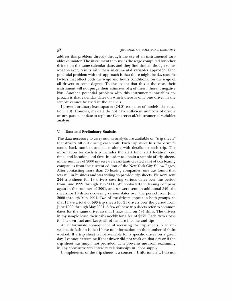
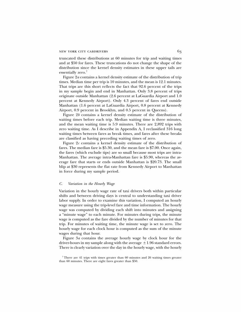
Figure 2 contains kernel density estimates of the distributions of triptimes, waiting times, and fares for the 13,464 trips in my sample. I have
5 Income per day is the sum of fares. Tip income is not measured or accounted for.6 All kernel density estimates in this study use the Epanechnikov kernel. The bandwidths
are listed in the figures.

Fig. 1.—Distributions of hours, income, and average wage by shift: a, hours worked ina shift; b, shift income; c, shift average hourly wage.
Fig. 2.—Kernel density estimates of a, trip times, b, waiting times, and c, fares
new york city cabdrivers 63
truncated these distributions at 60 minutes for trip and waiting timesand at $50 for fares. These truncations do not change the shape of thedistribution since the kernel density estimates in these upper tails areessentially zero.7
Figure 2a contains a kernel density estimate of the distribution of triptimes. Median time per trip is 10 minutes, and the mean is 12.1 minutes.That trips are this short reflects the fact that 92.6 percent of the tripsin my sample begin and end in Manhattan. Only 3.8 percent of tripsoriginate outside Manhattan (2.6 percent at LaGuardia Airport and 1.0percent at Kennedy Airport). Only 4.3 percent of fares end outsideManhattan (1.6 percent at LaGuardia Airport, 0.8 percent at KennedyAirport, 0.9 percent in Brooklyn, and 0.5 percent in Queens).
Figure 2b contains a kernel density estimate of the distribution ofwaiting times before each trip. Median waiting time is three minutes,and the mean waiting time is 5.9 minutes. There are 2,892 trips withzero waiting time. As I describe in Appendix A, I reclassified 316 longwaiting times between fares as break times, and fares after these breaksare classified as having preceding waiting times of zero.
Figure 2c contains a kernel density estimate of the distribution offares. The median fare is $5.30, and the mean fare is $7.00. Once again,the fares (which exclude tips) are so small because most trips are intra-Manhattan. The average intra-Manhattan fare is $5.90, whereas the av-erage fare that starts or ends outside Manhattan is $20.73. The smallblip at $30 represents the flat rate from Kennedy Airport to Manhattanin force during my sample period.
C. Variation in the Hourly Wage
Variation in the hourly wage rate of taxi drivers both within particularshifts and between driving days is central to understanding taxi driverlabor supply. In order to examine this variation, I computed an hourlywage measure using the trip-level fare and time information. The hourlywage was computed by dividing each shift into minutes and assigninga “minute wage” to each minute. For minutes during trips, the minutewage is computed as the fare divided by the number of minutes for thattrip. For minutes of waiting time, the minute wage is set to zero. Thehourly wage for each clock hour is computed as the sum of the minutewages during that hour.
Figure 3a contains the average hourly wage by clock hour for thedriver-hours in my sample along with the average �1.96 standard errors.There is clearly variation over the day in the hourly wage, with the hourly
7 There are 41 trips with times greater than 60 minutes and 26 waiting times greaterthan 60 minutes. There are eight fares greater than $50.

64 journal of political economy
Fig. 3.—Hourly wage, by clock hour: a, hourly wage; b, number of shifts and wage
wage rising from noon through midnight and falling between midnightand noon, with a temporary peak during the morning rush hour. Thevariation around the average wage for the early morning hours is rel-atively large because of the smaller number of driver-hours in my sampleduring that part of the day.
Figure 3b overlays the plot of the average hourly wage by clock hourwith a plot of the number of driver-hours in my sample by clock hour.While it is not the case that I have a random selection of cabs on thestreets of Manhattan at any point during the day, my trip sheets doprovide some evidence on variation over the day in the number of cabson the street. The minimum is at 6:00 a.m., after which the number ofdriver-hours increases through 1:00 p.m. The number of driver-hoursdrops sharply at 4:00 p.m. and 5:00 p.m., likely reflecting the changeof shifts, before increasing to the daily maximum at 7:00 p.m. Subse-quently, the number of driver-hours drops consistently through 6:00a.m.
It is interesting that the hourly wage is much less variable over theday than the supply of driver-hours. The number of driver-hours rangesfrom one at 6:00 a.m. to 249 at 7:00 p.m., whereas the average wagevaries from $18.75 at noon to $25.47 at 11:00 p.m.8 This pattern is
8 The wage is even higher at $26.30 at 5:00 a.m., but this is based on only two driver-hours.

new york city cabdrivers 65
TABLE 1Analysis of Variance of Hourly Wage
Variable (1) (2) (3) (4) (5) (6) (7) (8)
Driver identification x x x x xHour of day x x x x xDay of week x x x x xHour of day # day
of week x x x x xWeather x x xDate x x xDate # driver
identification xDegrees of freedom
used 0 20 141 161 165 315 470 7012R .00 .05 .15 .17 .17 .15 .28 .35
RMSE 6.67 6.51 6.31 6.25 6.24 6.49 6.17 6.12
Note.—The statistics in the table are based on linear regressions with dummy variables included for the indicatedcategories in each column. The sample used 3,025 hours for which all 60 minutes are either part of a trip or waitingtime between trips. Hours that include a break are excluded. The weather variables include hourly rainfall, daily snowfall,an indicator for minimum temperature below 30 degrees, and an indicator for maximum temperature greater than orequal to 80 degrees.
consistent with the number of drivers adjusting to daily fluctuations inthe pattern of demand.9 The lower wage at midday may reflect shortlunch breaks not recorded as such by drivers.
Table 1 contains the analysis of variance results from a series of re-gressions of the hourly wage on a sequence of sets of variables. Column1 refers to a regression with only a constant. The RMSE of this regression(the standard deviation of the wage) is 6.67. Controlling for driver fixedeffects (col. 2) accounts for only 5 percent of the variation in the hourlywage, and the RMSE is reduced slightly to 6.51. Controlling for the hourof the day, the day of the week, and their interaction (col. 3) accountsfor 15 percent of the variation in the hourly wage, and controlling driverfixed effects along with the hour of the day, the day of the week, andtheir interaction (col. 4) accounts for 17 percent of the hourly wagevariation.
I controlled additionally for the weather (four variables: [1] hourlyrainfall, [2] daily snowfall, [3] daily low temperature less than 30 degreesFahrenheit, and [4] daily high temperature greater than or equal to 80degrees Fahrenheit) in column 5. These variables do not improve the
substantially, but the hourly wage is significantly related to the2Rweather measures ( ). Specifically, the hourly wage is $1.04 lowerp p .033
9 Oettinger (1999) models the labor supply (participation) decisions of stadium vendorsacross days as a function of predictable fluctuations in demand. His model takes intoaccount the facts that other vendors are making similar decisions and that these decisionsaffect own income. Oettinger’s data include the labor supply of all vendors. The analogousparticipation data for New York City taxi drivers would include the labor supply of alldrivers. I do not have access to such data.
66 journal of political economy
TABLE 2Autocorrelations of Hourly Wage
Period (1) (2) Observations
0 1.0 1.0 3,0251 .0687* �.0369 2,2322 .0984 .0241 1,6523 .0625* �.0072 1,3124 .0261 �.0351 1,0345 .0644 .0079 7856 .1354* .1297* 5397 �.0082 �.0290 334
Note.—Col. 1 contains autocorrelations of hourly wages indexed by hour on shift. Col.2 contains autocorrelations of residuals of hourly wages indexed by hour on shift. Theresiduals are calculated from a regression of the hourly wage on a set of driver fixed effectsand a set of hour-of-day fixed effects.
* Significantly different from zero at the .05 level.
on hot days ( ), $0.49 lower on cold days ( ), and, sur-p p .007 p p .158prisingly, $0.94 lower for each 0.1 inch of hourly rain ( ).p p .103
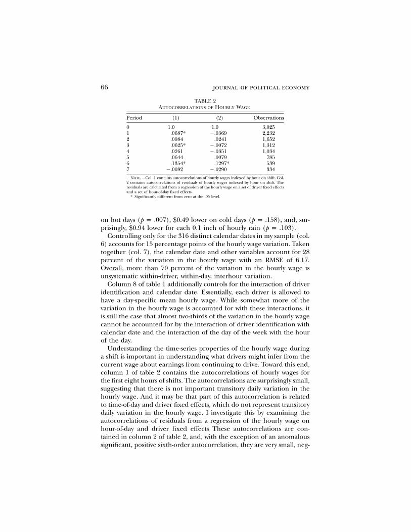
Controlling only for the 316 distinct calendar dates in my sample (col.6) accounts for 15 percentage points of the hourly wage variation. Takentogether (col. 7), the calendar date and other variables account for 28percent of the variation in the hourly wage with an RMSE of 6.17.Overall, more than 70 percent of the variation in the hourly wage isunsystematic within-driver, within-day, interhour variation.
Column 8 of table 1 additionally controls for the interaction of driveridentification and calendar date. Essentially, each driver is allowed tohave a day-specific mean hourly wage. While somewhat more of thevariation in the hourly wage is accounted for with these interactions, itis still the case that almost two-thirds of the variation in the hourly wagecannot be accounted for by the interaction of driver identification withcalendar date and the interaction of the day of the week with the hourof the day.
Understanding the time-series properties of the hourly wage duringa shift is important in understanding what drivers might infer from thecurrent wage about earnings from continuing to drive. Toward this end,column 1 of table 2 contains the autocorrelations of hourly wages forthe first eight hours of shifts. The autocorrelations are surprisingly small,suggesting that there is not important transitory daily variation in thehourly wage. And it may be that part of this autocorrelation is relatedto time-of-day and driver fixed effects, which do not represent transitorydaily variation in the hourly wage. I investigate this by examining theautocorrelations of residuals from a regression of the hourly wage onhour-of-day and driver fixed effects These autocorrelations are con-tained in column 2 of table 2, and, with the exception of an anomaloussignificant, positive sixth-order autocorrelation, they are very small, neg-
new york city cabdrivers 67
TABLE 3Labor Supply Function Estimates: OLS Regression of Log Hours
Variable (1) (2) (3)
Constant 4.012(.349)
3.924(.379)
3.778(.381)
Log(wage) �.688(.111)
�.685(.114)
�.637(.115)
Day shift … .011(.040)
.134(.062)
Minimum temperature! 30
… .126(.053)
.024(.058)
Maximum temperature≥ 80
… .041(.055)
.055(.064)
Rainfall … �.022(.073)
�.054(.071)
Snowfall … �.096(.036)
�.093(.035)
Driver effects no no yesDay-of-week effects no yes yes
2R .063 .098 .198
Note.—The sample includes 584 shifts for 21 drivers. The dependent variable is log hours worked(driving time plus time between fares excluding declared breaks and breaks between fares one houror longer). The mean of the dependent variable is 1.84. Standard errors are in parentheses.
ative, and not significantly different from zero. This suggests little orno role for transitory daily shocks to the hourly wage.
While there is significant day-to-day variation in the hourly wage, theresults in tables 1 and 2 suggest that most variation in the wage appearsto be nonforecastable within-day variation. On this basis, predictinghours of work with a model that assumes a fixed hourly wage rate duringthe day does not seem appropriate.
VI. Estimation of the Labor Supply Models
I begin the presentation of estimates of labor supply models by esti-mating the labor supply model used by Camerer et al. (1997) and byChou (2000) and formulated in equation (10). I then implement theprobit model of the probability of stopping based on the latent variabledefined in equation (9).
A. Estimation of the Log Hours Function
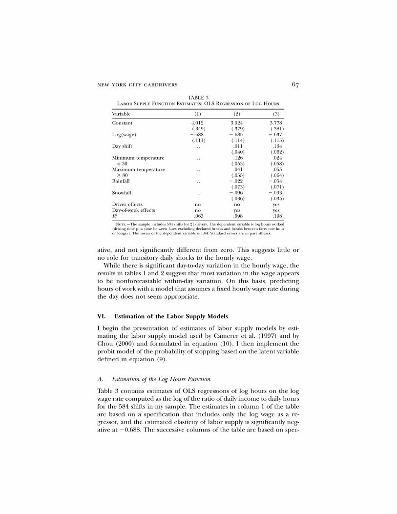
Table 3 contains estimates of OLS regressions of log hours on the logwage rate computed as the log of the ratio of daily income to daily hoursfor the 584 shifts in my sample. The estimates in column 1 of the tableare based on a specification that includes only the log wage as a re-gressor, and the estimated elasticity of labor supply is significantly neg-ative at �0.688. The successive columns of the table are based on spec-

68 journal of political economy
ifications that include additional regressors. The specification in column2 includes controls for shift, day of the week, and four measures of thedaily weather. The estimated wage elasticity is virtually unchanged inthis specification. The results indicate no difference in hours workedbetween the day shift and the night shift. The estimates of the coeffi-cients of the weather measures suggest that shifts are longer on colddays and shorter on snowy days. Rainfall is not statistically significantlyrelated to shift length. The estimates in column 3 additionally controlfor driver fixed effects. There are significant differences across driversin hours worked ( ), but accounting for these differences doesp ! .0005not have a substantial effect on the estimated negative wage elasticity.Interestingly, when driver fixed effects are accounted for, the day shiftindicator is significantly negative, suggesting that, when a specific drivermoves from the night shift to the day shift, hours increase by about 13percent and vice versa. Finally, controlling for the weather along withdriver fixed effects in column 4 suggests that, while hours are unrelatedto temperature extremes or rainfall, drivers do work fewer hours whenit has snowed.
The key consistent finding is that there appears to be a substantialnegative elasticity of labor supply, as is found by Camerer et al.10 How-ever, there is strong potential for negative bias in the estimated elasticitybecause the wage is computed mechanically using the inverse of hoursworked. Additionally, since the wage is not constant over the workingday and is not highly autocorrelated hour to hour, it is not likely thatthe wage measured this way can be considered parametric to the laborsupply decision. Thus I do not consider estimates of a labor supplyelasticity derived using this daily regression approach to be reliable,even if a convincing instrument for the wage were available.
B. Estimation of the Probit Optimal Stopping Model
The probability that a driver ends his shift increases sharply as hoursand income accumulate. Panel A of table 4 contains the simple empiricalhazard of a driver stopping after a trip ending in a given time intervalsince the start of the shift. The likelihood that a driver will stop increasesfrom 0.5 percent in the first two hours to 15 percent in hour 8 and toover 25 percent by hour 12. Note that since there are multiple tripsending in any given hour, the probability that a driver stops in a givenhour is considerably larger than the single-trip hazards listed in thetable. Panel B of table 4 contains the simple empirical hazard of a driver
10 The similarity of our findings is important because it implies that any differences inresults that I find using other empirical models are due to differences in analytic approachrather than to differences in the data used.

new york city cabdrivers 69
TABLE 4Empirical Hazard of Stopping by Hours and
by Income
A B
Hour Hazard Income ($) Hazard
≤ 2 .0050 ! 25 .00163–5 .0244 25–49 .00786 .0517 50–74 .01497 .0992 75–99 .02288 .1467 100–124 .03389 .1147 125–149 .059610 .1609 150–174 .111111 .2450 175–199 .1477≥ 12 .2636 200–224 .1283
≥ 225 .1977
Note.—Based on the sample of 13,461 trips in 584 shifts for 21drivers. These figures are the probability of stopping after a trip inthe designated hour of the shift or with total income in the indi-cated range conditional on not having stopped earlier.
stopping after a trip ending with shift income in the given interval. Thelikelihood that a driver will stop increases from 0.16 percent when thedriver has earned less than $25 to 11 percent when the driver has earned$150–$174. Analogously to the case of hours, there are likely to bemultiple trips ending in any of these intervals so that the probabilitythat a driver stops with income in any particular interval is considerablylarger than the single-trip hazards listed in the table.
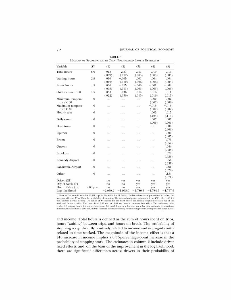
In Section IV, I outlined a probit model of the probability that a driverstops after a given trip as a function of hours worked to that point,income earned to that point, current location, weather, and fixed effectsfor driver, calendar date, hour of the day, and day of the week. Thelatent variable defined in equation (9) forms the basis for estimationof this model. Table 5 contains estimates of this model in which incomeand hours are constrained to enter linearly.11 The normalized probitestimate is , where is the standard normal density. Givenb̂ 7 f(X *b) f(7)that the probability that a shift will end early in the shift is very smalland there are more trips early than late, evaluating the density at themean for this normalization could be misleading.12 As a result, I selectedreasonable values for the key variables. I evaluate the marginal effectof a variable on the probability of quitting after eight total hours (5.5trip hours, 2.5 waiting hours, 0.5 break hour) on a dry day with moderatetemperatures in midtown Manhattan at 2:00 p.m.
The estimates in column 1 of table 5 contain only the hours measures
11 This constraint is relaxed in table 6.12 The probit specification naturally accounts for this nonlinearity since the marginal
effect of any given variable on the probability of quitting is smaller in the tails of thedistribution.
70 journal of political economy
TABLE 5Hazard of Stopping after Trip: Normalized Probit Estimates
Variable X* (1) (2) (3) (4) (5)
Total hours 8.0 .013(.009)
.037(.012)
.011(.005)
.010(.005)
.010(.005)
Waiting hours 2.5 .010(.010)
�.005(.012)
.001(.006)
.004(.006)
.004(.005)
Break hours .5 .006(.008)
�.015(.011)
�.003(.005)
�.001(.005)
�.002(.005)
Shift income�100 1.5 .053(.022)
.036(.030)
.014(.015)
.016(.016)
.011(.015)
Minimum tempera-ture ! 30
.0 … … … .002(.007)
.002(.006)
Maximum tempera-ture ≥ 80
.0 … … … �.016(.007)
�.016(.007)
Hourly rain .0 … … … .005(.124)
.015(.113)
Daily snow .0 … … … .007(.006)
.007(.005)
Downtown .0 … … … … .000(.006)
Uptown .0 … … … … .000(.005)
Bronx .0 … … … … .075(.057)
Queens .0 … … … … .044(.038)
Brooklyn .0 … … … … .078(.036)
Kennedy Airport .0 … … … … .056(.031)
LaGuardia Airport .0 … … … … .061(.029)
Other .0 … … … … .134(.071)
Driver (21) no yes yes yes yesDay of week (7) no no yes yes yesHour of day (19) 2:00 p.m. no no yes yes yesLog likelihood �2,039.2 �1,965.0 �1,789.5 �1,784.7 �1,767.6
Note.—The sample includes 13,461 trips in 584 shifts for 21 drivers. Probit estimates are normalized to reflect themarginal effect at of X on the probability of stopping. The normalized probit estimate is , where f(7) isˆX* b 7 f(X*b)the standard normal density. The values of chosen for the fixed effects are equally weighted for each day of theX*week and for each driver. The hours from 5:00 a.m. to 10:00 a.m. have a common fixed effect. The evaluation pointis after 5.5 driving hours, 2.5 waiting hours, and 0.5 break hour in a dry hour on a day with moderate temperaturesin midtown Manhattan at 2:00 p.m. Robust standard errors accounting for clustering by shift are reported in parentheses.
and income. Total hours is defined as the sum of hours spent on trips,hours “waiting” between trips, and hours on break. The probability ofstopping is significantly positively related to income and not significantlyrelated to time worked. The magnitude of the income effect is that a$10 increase in income implies a 0.53-percentage-point increase in theprobability of stopping work. The estimates in column 2 include driverfixed effects, and, on the basis of the improvement in the log likelihood,there are significant differences across drivers in their probability of

new york city cabdrivers 71
quitting. Interestingly, after one accounts for interdriver differences, theprobability of quitting is not significantly related to income but is sig-nificantly related to total hours. A one-hour increase in total time isassociated with a 3.7-percentage-point increase in the probability of quit-ting. Given that the probability of stopping for trips ending in the eighthhour is 0.14, this is a substantial effect. In neither column 1 nor column2 do waiting hours or break hours have a significantly different effecton the probability of stopping work than hours on trips.
The estimates in column 3 additionally control for hour of day andday of week. The marginal effect of hours on the probability of stoppingis much lower in this specification, with a one-hour increase in totaltime increasing the probability of quitting by 1.1 percentage points.This is not surprising, given the fact that shift start and end times tendto be concentrated in a relatively narrow range of clock hours. Themagnitude and statistical significance of the marginal effect of incomeon the probability of stopping is reduced further by the additional con-trol variables.
The estimates in column 4 add the weather measures. The only sta-tistically significant finding is that the probability of stopping work is1.6 percentage points lower on hot days. Perhaps surprisingly, givenanecdotal reports of the difficulty of finding taxis in rainy weather, thereis no relationship between hourly rainfall and the probability of stop-ping. This would suggest that reported difficulty in finding a taxi inrainy weather is due to increased demand.13
Finally, the estimates in column 5 include controls for geographiclocation at the end of the trip. The omitted location is midtown Man-hattan (between Fourteenth Street and Fifty-ninth Street). The generalpattern is clear. Drivers are substantially more likely to stop workingafter a fare that takes them outside Manhattan. For example, drivershave a 6.1-percentage-point higher probability of stopping work after afare to LaGuardia Airport, located in Queens. The reason may be thatdrivers are closer to home in the outlying boroughs. Controlling forlocation has an insubstantial effect on the coefficients of the key hoursand income measures.
A potential problem with the estimates in table 5 is that hours andincome are constrained to affect the underlying latent variable linearly.While the probit function introduces a particular form of nonlinearitythat reduced the marginal effects in the tails of the distribution, the
13 The results reported in the discussion of table 1 suggest that the hourly wage is lowerin rainy weather. This is not consistent with an increase in demand. One possible expla-nation might be that demand does increase when it is raining, but there is also a rain-induced slowdown in traffic that increases trip times for a given distance traveled andfare. Simple tabulation of the trip-level data shows that dollars earned per minute with afare in the cab is statistically significantly lower by about $0.04 when it is raining.
72 journal of political economy
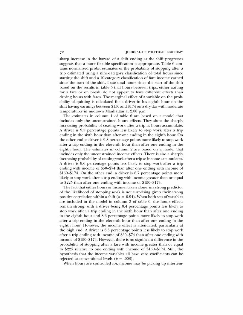
sharp increase in the hazard of a shift ending as the shift progressessuggests that a more flexible specification is appropriate. Table 6 con-tains normalized probit estimates of the probability of stopping after atrip estimated using a nine-category classification of total hours sincestarting the shift and a 10-category classification of fare income earnedsince the start of the shift. I use total hours since the start of the shiftbased on the results in table 5 that hours between trips, either waitingfor a fare or on break, do not appear to have different effects thandriving hours with fares. The marginal effect of a variable on the prob-ability of quitting is calculated for a driver in his eighth hour on theshift having earnings between $150 and $174 on a dry day with moderatetemperatures in midtown Manhattan at 2:00 p.m.
The estimates in column 1 of table 6 are based on a model thatincludes only the unconstrained hours effects. They show the sharplyincreasing probability of ceasing work after a trip as hours accumulate.A driver is 9.5 percentage points less likely to stop work after a tripending in the sixth hour than after one ending in the eighth hour. Onthe other end, a driver is 9.8 percentage points more likely to stop workafter a trip ending in the eleventh hour than after one ending in theeighth hour. The estimates in column 2 are based on a model thatincludes only the unconstrained income effects. There is also a sharplyincreasing probability of ceasing work after a trip as income accumulates.A driver is 9.6 percentage points less likely to stop work after a tripending with income of $50–$74 than after one ending with income of$150–$174. On the other end, a driver is 8.7 percentage points morelikely to stop work after a trip ending with income greater than or equalto $225 than after one ending with income of $150–$174.
The fact that either hours or income, taken alone, is a strong predictorof the likelihood of stopping work is not surprising given their strongpositive correlation within a shift ( ). When both sets of variablesr p 0.94are included in the model in column 3 of table 6, the hours effectsremain strong, with a driver being 8.4 percentage points less likely tostop work after a trip ending in the sixth hour than after one endingin the eighth hour and 8.6 percentage points more likely to stop workafter a trip ending in the eleventh hour than after one ending in theeighth hour. However, the income effect is attenuated, particularly atthe high end. A driver is 6.3 percentage points less likely to stop workafter a trip ending with income of $50–$74 than after one ending withincome of $150–$174. However, there is no significant difference in theprobability of stopping after a fare with income greater than or equalto $225 relative to one ending with income of $150–$174. Still, thehypothesis that the income variables all have zero coefficients can berejected at conventional levels ( ).p p .008
When hours are controlled for, income may be picking up intertem-

TABLE 6Hazard of Stopping after Trip: Normalized Probit Estimates
Variable (1) (2) (3) (4)
Hour:≤ 2 �.142
(.014)… �.137
(.017)�.042(.012)
3–5 �.122(.014)
… �.108(.017)
�.028(.010)
6 �.095(.015)
… �.084(.018)
�.026(.009)
7 �.048(.016)
… �.041(.018)
�.012(.008)
9 �.032(.021)
… �.034(.022)
�.006(.010)
10 .014(.025)
… .011(.033)
.031(.020)
11 .098(.038)
… .086(.051)
.085(.036)
≥ 12 .117(.063)
… .109(.075)
.119(.060)
Income ($):! 5 … �.109
(.010)�.121(.022)
�.036(.014)
25–49 … �.103(.010)
�.067(.027)
.005(.022)
50–74 … �.096(.010)
�.063(.021)
�.002(.014)
75–99 … �.088(.010)
�.065(.020)
�.010(.011)
100–124 … �.077(.011)
�.053(.018)
�.009(.009)
125–149 … �.052(.011)
�.035(.017)
�.007(.008)
175–199 … .037(.018)
.014(.021)
.011(.010)
200–224 … .017(.020)
�.022(.025)
.006(.013)
≥ 225 … .087(.019)
.009(.032)
.015(.018)
Driver (21) no no no yesDay of week (7) no no no yesHour of day (19) no no no yesLocation (9) no no no yesWeather (4) no no no yesp-value:
Hours p 0 .000 … .000 .000Income p 0 … .000 .008 .281
Log likelihood �2,028.9 �2,058.7 �2,016.5 �1,753.1
Note.—The sample includes 13,461 trips in 584 shifts for 21 drivers. Probit estimates are normalized to reflect themarginal effect at of X on the probability of stopping. The normalized probit estimate is , where f(7) isˆX* b 7 f(X*b)the standard normal density. The values of chosen for the fixed effects are equally weighted for each day of theX*week and driver. The hours from 5:00 a.m. to 10:00 a.m. have a common fixed effect. The evaluation point is at eighttotal hours with income of $150–$174 in a dry hour on a day with moderate temperatures in midtown Manhattan at2:00 p.m. Robust standard errors accounting for clustering by shift are reported in parentheses.
74 journal of political economy
poral and interdriver differences in the value of continuing to drive. Inorder to address this possibility, the estimates in column 4 of table 6are derived from a model that includes additional controls for driver,day of the week, hour of the day, weather, and geographic location. AsI showed in table 5, these variables are all important determinants ofthe probability of stopping. Interestingly, hours worked remains an im-portant factor in the stopping decision, but the pattern is changedsomewhat. The differences are much smaller early in the shift, with onlya 2.5-percentage-point reduction in the likelihood of stopping in thesixth hour relative to the eighth hour. However, the differences late inthe shift are unchanged, with an 8.5-percentage-point increase in thelikelihood of stopping in the eleventh hour relative to the eighth hour.
Income is no longer a factor. Only the coefficient on income lessthan or equal to $25 is significantly different from zero, and its mag-nitude suggests only a 3.6-percentage-point reduction relative to the$150–$174 category. All other estimates on the income categories aresmaller along with not being significantly different from zero. The hy-pothesis that all the income coefficients are zero cannot be rejected atconventional levels ( ).p p .28
The clear conclusion from this analysis is that hours of work is acentral determinant of the stopping decision but daily income is notrelated to the stopping decision. Thus there are not important dailyincome effects, and the evidence is not consistent with target earningsbehavior by taxi drivers.
C. Labor Supply Models for Specific Drivers
A restriction implicit in the analysis of the previous section is that driversare assumed to follow a common behavioral model aside from an in-tercept shift in the underlying function determining the probability ofstopping after a trip. This could be misleading, particularly if somedrivers are target earners and other are not or if drivers are targetearners but have heterogeneous targets. In order to investigate the im-portance of driver heterogeneity, I estimate separate stopping modelsfor the six drivers for whom I have more than 40 trip sheets.
This analysis is complicated by the fact that drivers are fairly consistentacross days in their starting times, and while their ending times showmore variation as a result of the labor supply decision, individual driversdo not tend to “cover the clock.” Shifts for particular drivers tend toend in a fairly narrow time window. As a result, it is not feasible tocontrol for clock hour in the analysis. This is a problem because clockhour is an important component of drivers’ calculations of the value ofcontinuing to work. The inability to control directly for clock hourmakes difficult the interpretation of estimates of the effect of cumulative
new york city cabdrivers 75
TABLE 7Driver-Specific Hazard of Stopping after Trip: Normalized Probit Estimates
Variable
Driver
4 10 16 18 20 21
Hours .073(.060)
.056(.047)
.043(.015)
.010(.007)
.195(.045)
.198(.030)
Income�100 .178(.167)
.039(.059)
.064(.041)
.048(.020)
�.160(.123)
�.002(.150)
Number of shifts 40 45 70 72 46 46Number of trips 884 912 1,754 2,023 1,125 882Log likelihood �124.1 �116.0 �221.1 �260.6 �123.4 �116.9
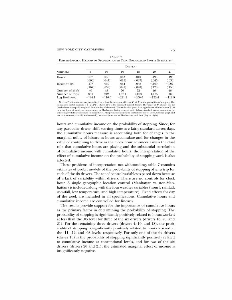
Note.—Probit estimates are normalized to reflect the marginal effect at of X on the probability of stopping. TheX*normalized probit estimate is , where f(7) is the standard normal density. The values of chosen for theb̂ 7 f(X*b) X*fixed effects are equally weighted for each day of the week. The evaluation point is at eight hours with income of $150in a dry hour of moderate temperature in Manhattan during a night shift. Robust standard errors accounting forclustering by shift are reported in parentheses. All specifications include controls for day of week, weather (high andlow temperatures, rainfall, and snowfall), location (in or out of Manhattan), and shift (day or night).
hours and cumulative income on the probability of stopping. Since, forany particular driver, shift starting times are fairly standard across days,the cumulative hours measure is accounting both for changes in themarginal utility of leisure as hours accumulate and for changes in thevalue of continuing to drive as the clock hour advances. Given the dualrole that cumulative hours are playing and the substantial correlationof cumulative income with cumulative hours, the interpretation of theeffect of cumulative income on the probability of stopping work is alsoaffected.
These problems of interpretation not withstanding, table 7 containsestimates of probit models of the probability of stopping after a trip foreach of the six drivers. The set of control variables is pared down becauseof a lack of variability within drivers. There are no controls for clockhour. A single geographic location control (Manhattan vs. non-Man-hattan) is included along with the four weather variables (hourly rainfall,snowfall, low temperature, and high temperature). Fixed effects for dayof the week are included in all specifications. Cumulative hours andcumulative income are controlled for linearly.
The results provide support for the importance of cumulative hoursas the primary factor in determining the probability of stopping. Theprobability of stopping is significantly positively related to hours workedat less than the .05 level for three of the six drivers (drivers 16, 20, and21). For the remaining three drivers (drivers 4, 10, and 18), the prob-ability of stopping is significantly positively related to hours worked atthe .11, .12, and .08 levels, respectively. For only one of the six drivers(driver 18) is the probability of stopping significantly positively relatedto cumulative income at conventional levels, and for two of the sixdrivers (drivers 20 and 21), the estimated marginal effect of income isinsignificantly negative.

76 journal of political economy
Overall, the stopping rules for these six individual drivers are consis-tent with the neoclassical model of labor supply and are not consistentwith the target earnings model.
D. Reanalysis of the Camerer et al. TRIP Data
Given the sharp contrast between my conclusion that cabdriver worktime on a given day is consistent with a neoclassical intertemporal laborsupply model and inconsistent with a target earnings model and theopposite conclusion of Camerer et al., it is important to understand thebasis of the difference. Clearly, the statistical and conceptual modelsused are very different, and these differences in approach likely accountfor the difference in findings. However, the samples of trip sheets usedalso differ, and it is possible that the difference in data could accountfor the difference in results.
I have already applied the Camerer et al. regression approach to mydata by estimating log hours regressions by OLS (table 3), and the resultsshow the same significantly negative labor supply elasticity found in theearlier study. The remaining question is whether, when applying mystatistical model to the Camerer et al. data, I find results consistent withthe estimates reported in tables 5 and 6.
Camerer et al. supplied me with their TRIP data, a sample of 70 tripsheets for 13 drivers that can be used to estimate my probit stoppingmodel. They report substantial first- and second-order autocorrelationsof the hourly wage of approximately 0.5, which is evidence consistentwith there being significant daily fluctuations in the hourly wage. Thisstands in sharp contrast to my calculation of the first- and second-orderautocorrelations of the hourly wage in my data of 0.07 and 0.10, re-spectively (table 2), which are not consistent with there being significantdaily fluctuations in the hourly wage. I recalculated the hourly wage inthe TRIP data using the same method I describe in Section V.C, and Icomputed the autocorrelations. My calculations yield autocorrelationsthat differ substantially from those presented by Camerer et al. for thesame data. I find first- and second-order autocorrelations of the hourlywage of 0.17 and 0.22, respectively.14 While these autocorrelations aresomewhat larger than those found in my data, they are not nearly aslarge as those reported by Camerer et al., and they do not providesupport for important daily fluctuations in the hourly wage.
Next, I estimate the probit stopping model using the Camerer et al.TRIP data. Of the eight drivers in the TRIP sample, five are observedfor only a single shift. Since I include driver fixed effects in the speci-
14 As in my data, autocorrelations of hourly wage residuals from the Camerer et al. dataare insignificantly negative.

new york city cabdrivers 77
TABLE 8Hazard of Stopping after Trip: Camerer et al. TRIP Data: Sixth or Later Hour
Normalized Probit Estimates
VariableAll(1)
!MedianExperience
(2)
≥MedianExperience
(3)
LowExperience
(4)
MediumExperience
(5)
HighExperience
(6)
Total hours .101(.030)
.003(.004)
.102(.044)
.001(.004)
.307(.112)
.098(.049)
Shift income�100 .055(.119)
.016(.018)
�.136(.101)
.063(.122)
�.515(.342)
�.027(.116)
Driver fixed effects yes yes yes yes yes yesNumber of drivers 8 3 5 1 4 3Number of shifts 65 26 39 10 33 22Number of trips 554 239 315 60 319 175Log likelihood �144.2 �55.7 �83.4 �20.0 �70.9 �40.6
Note.—Probit estimates in the bottom rows are normalized to reflect the marginal effect at (eight hours of workX*and $125 in earnings) of a change in X on the probability of stopping. The normalized probit estimate is ,b̂ 7 f(X*b)where f(7) is the standard normal density. The reported standard errors (in parentheses) are computed by applyingthe delta method to robust standard errors of b that account for clustering by driver/shift.
fication, I drop these five drivers from my reanalysis. With only 65 shiftsfor eight drivers, there is not substantial variation in shift starting time.All shifts started between 1:00 p.m. and 8:00 p.m., and 56 of the 65shifts started between 4:00 p.m. and 7:00 p.m. This makes it difficult toidentify hours worked on a shift separately from clock hour. None ofthe 65 trips ended until more than six hours had been worked. As aresult of these factors, I estimate the stopping model including only the554 trips that began after working six hours, and I measure hours andincome linearly without any control for hour of the day or day of theweek. In addition to the linear measures of hours worked and shiftincome, the model includes only driver fixed effects.
Column 1 of table 8 contains normalized probit estimates of thestopping model using the Camerer et al. TRIP data. There is a significantpositive relationship between the probability of stopping after a trip andcumulative hours. The point estimate suggests that each additional hourof work increases the likelihood of stopping after a trip by 10 percentagepoints. There is no significant relationship between cumulative shiftincome and the probability of stopping. This pattern of evidence isconsistent with estimates of the stopping model based on my data andwith a standard neoclassical intertemporal labor supply model. Theredo not appear to be strong income effects in the TRIP data.
The role of experience in the Camerer et al. TRIP data.—Camerer et al.suggest that their finding of a negative wage elasticity of labor supplymight be the result of income targeting by less experienced drivers, withmore experienced drivers behaving in a manner consistent with theneoclassical model. They investigate this by breaking their sample byexperience level using the hack license number assigned consecutivelyby the New York City Taxi and Limousine Commission. They break the
78 journal of political economy
sample at the median hack number, ranging in their sample from 50,893to 610,069, with higher numbers indicating less experience. When Ca-merer et al. reestimate their OLS model separately for the high- andlow-experience samples, they find a significant negative labor supplyelasticity (�0.841) for the low-experience group and a positive laborsupply elasticity for the high-experience group (0.613).
I reestimated the probit model using the TRIP data separately foreach of the two experience groups defined by Camerer et al. The resultsof this estimation are in columns 2 and 3 of table 8. They show norelationship between the probability of stopping and shift income foreither experience group. Interestingly, there is a significant relationshipbetween hours worked and the probability of stopping for the moreexperienced group but not for the less experienced group. This suggeststhat there might be some experience-related learning about optimallabor supply behavior.
Using the median hack number to break the sample may not yield asharp distinction in experience given that there is not a sharp break inthe sample at the median (450,079). Fully nine of the 13 drivers havehack numbers in the 400,000 range. There are three more experienceddrivers with hack numbers less than 400,000 (50,893, 96,013, and318,867) and one less experienced driver with a hack number of610,069. All five of the drivers with single shifts in the sample have hacknumbers in the 400,000 range. The eight drivers with multiple shiftscan be more naturally divided into three groups: (1) low experience(≥ 500,000), (2) medium experience (400,000–499,999), and (3) highexperience (! 400,000).
I reestimated the probit model using the TRIP data separately foreach of these three experience groups. The results of this estimationare in columns 4–6 of table 8. The results are interesting. There is asignificant positive relationship between hours worked and the proba-bility of stopping after a trip for both the medium- and high-experiencegroups. There are negative and insignificant estimates of the relation-ship between cumulative income and the probability of stopping forboth of these groups of drivers. For the least experienced driver (alonein the low-experience group), there is no significant relationship ofeither hours or income with the probability of stopping.
The overall pattern of evidence by experience level suggests indirectlythat Camerer et al.’s experience result is due to the single very lowexperienced driver (hack number of 610,069, more than 130,000 higherthan the next more experienced driver). On the basis of a single driver,I am reluctant to conclude that taxi drivers learn from experience tobehave optimally whereas less experienced drivers are more likely to betarget earners.
new york city cabdrivers 79
VII. Final Remarks: Tomorrow Is Another Day
The results of the probit stopping models I estimate, whether appliedto my taxi data or to the Camerer et al. TRIP data, show consistentlythat the probability of stopping daily work after a particular trip isstrongly related to hours worked to that point and not significantlyrelated to cumulative income earned. This pattern is consistent with aconventional neoclassical intertemporal labor supply model with weakor nonexistent income effects due to transitory changes to the marginaldaily wage. There is no evidence either for important income effects orfor target earnings behavior. These findings are in sharp contrast to thefinding of negative daily wage elasticities of labor supply reported byCamerer et al. (1997).
While I estimated a model of labor supply, I did not estimate a wageelasticity of labor supply. In order to estimate such an elasticity, therewould need to be an exogenous permanent or transitory shift in thegeneral level of earnings opportunities. Some natural experiment (suchas Oettinger [1999]) or randomized experiment (such as Fehr andGoette [2002]) that yielded changes to daily earnings opportunitieswould provide the right sort of variation.
A complete analysis of the labor supply response to changes in earn-ings opportunities needs to examine both daily hours responses andresponses in the number of days worked (the participation margin).Owing to data limitations, I cannot investigate the daily labor supply oftaxi drivers on the participation margin, and my analysis is restricted tothe daily hours margin.15 Despite this limitation, the fact that I find noevidence of a daily income effect on hours worked leads me to concludethat the labor supply behavior of taxi drivers can be characterized by aconventional neoclassical intertemporal labor supply model.
Appendix A
Procedures for Cleaning Data
I perform several regularity checks to ensure that the trip sheets are internallyconsistent, and where they are not, I clean the data using a set of reasonablerules. I outline that process here. The main consistency checks are that (1) tripsmust start no earlier than the end of the previous trip and (2) trips must startbefore they end (have a positive duration). I also develop a set of rules to imputestarting or ending times for trips where such times are missing and fares wherefares are missing. For the most part, the trips on my trip sheets satisfy theserules and have nonmissing time and fare data. In the small number of cases in
15 Oettinger (1999) examines labor supply response on the participation margin in asetting in which daily hours are fixed. Fehr and Goette (2002) examine labor supplyresponse on both margins.
80 journal of political economy
which these rules are not satisfied or time or fare data are missing (about 1percent of trips), I use the following procedures.
1. I impute new trip times for 38 trips of zero duration. I start by computingthe length of time between the end of the previous trip and the start ofthe next trip. Clearly, the time of the “current” trip is no greater than thisavailable gap. I compute a predicted trip length based on a regression oftrip length on the fare and its square ( ). In almost all cases, this2R p 0.68predicted trip length is less than the available gap. I then center the pre-dicted trip length in the available gap and compute the implied adjustedstart and end times for the trip. In the handful of cases in which thepredicted trip length is longer than the gap (never by more than a fewminutes), I set the trip length equal to the available gap and compute theadjusted start and end times for the trip accordingly.
2. I impute new trip times for 52 cases in which one or both of the startingand ending times are missing. Most of these times are imputed using thesame predicted trip length defined above as a function of the fare. If thestart time is missing, it is computed as the end time minus the predictedtrip length. Analogously, if the end time is missing, it is computed as thestart time plus the predicted trip length. Where both times are missing,they are computed as defined above for trips of zero duration. There area handful of cases in which one or the other of the times is missing andthe fare is missing. In these cases, I predict trip length using a completeinteraction of starting and ending locations of the trip ( ).2R p 0.44
3. I adjust times where they are out of sequence. There are 83 cases in whicha trip apparently started before the previous trip ended. The mean overlapwas 2.7 minutes, and the maximum overlap was nine minutes. I adjust thesetimes by reducing the end time of the previous trip by one-half of theoverlap and increasing the start time of the current trip by one-half of theoverlap.
4. I impute fares for 45 cases in which the fare is missing. I impute fares inthese cases using predicted values from a regression of fare on trip lengthand a complete set of interactions of starting and ending locations( ). In the seven cases in which location is missing, I predict on2R p 0.83the basis of a model using only trip length ( ).2R p 0.64
5. I classify as breaks (nonwork time during the day) certain long waiting timesbetween fares. I classify as breaks (1) 195 periods of at least 30 minutesbetween a fare that ended in Manhattan and a fare that started in Man-hattan, (2) 112 periods of at least 60 minutes between fares that eitherstarted or ended outside Manhattan but did not end at either LaGuardiaor Kennedy Airport, and (3) nine periods of at least 120 minutes that endedat LaGuardia or Kennedy Airport.
6. I impute starting locations to 144 trips and ending locations to 223 tripswith missing or illegible locations. Where the starting location is missing,I assume that the starting location is the same as the ending location ofthe previous trip. Where the ending location is missing, I assume that theending location is the same as the starting location of the next trip. In casesin which the necessary information for imputation by these rules is notavailable, I examined the individual trip sheets and made an imputation-based on the “nearest” available locations, the size of the fares, and elapsedtime of the trip. Since over 96 percent of trips start in Manhattan and over95 percent of trips end in Manhattan, almost all the allocated locations arein Manhattan.
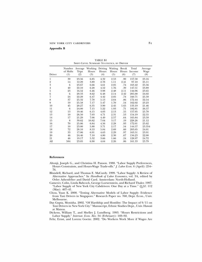
new york city cabdrivers 81
Appendix B
TABLE B1Shift-Level Summary Statistics, by Driver
Driver
Numberof Shifts
(1)
AverageTrips(2)
WorkingHours
(3)
DrivingHours
(4)
WaitingHours
(5)
BreakHours
(6)
TotalIncome
(7)
AverageWage(8)
1 39 23.56 6.85 4.32 2.53 .90 157.58 23.162 14 12.29 3.89 2.78 1.11 2.41 97.10 25.113 6 23.67 6.66 4.61 2.05 .74 163.42 25.564 40 22.10 6.28 4.52 1.76 .39 147.51 23.895 23 16.52 6.46 3.98 2.48 2.11 144.96 23.656 6 29.33 8.62 6.48 2.14 2.42 205.00 24.027 24 22.29 6.47 4.42 2.05 .74 160.71 25.598 37 25.32 7.78 5.13 2.64 .86 172.44 22.549 19 25.58 7.17 5.47 1.70 .54 162.02 23.2310 45 20.27 6.35 3.90 2.45 1.65 133.19 21.4611 6 24.00 7.15 5.22 1.93 .71 182.81 26.5712 13 19.46 6.15 4.03 2.13 .55 157.95 25.7813 10 26.50 7.03 4.71 2.31 .53 154.19 22.5514 17 21.29 7.06 4.49 2.57 .64 165.84 23.5915 8 39.62 10.82 7.64 3.17 .19 228.26 21.1216 70 25.06 6.84 4.56 2.28 .93 172.01 25.6217 10 23.00 5.88 3.71 2.17 .54 144.57 23.35418 72 28.10 8.53 5.84 2.69 .60 203.05 24.0119 33 17.06 6.91 4.63 2.29 .97 163.51 23.9120 46 24.46 7.10 4.80 2.30 .67 156.23 22.0021 46 19.17 5.32 3.66 1.66 .24 128.97 24.72All 584 23.05 6.90 4.64 2.26 .86 161.33 23.79
References
Altonji, Joseph G., and Christina H. Paxson. 1988. “Labor Supply Preferences,Hours Constraints, and Hours-Wage Trade-offs.” J. Labor Econ. 6 (April): 254–76.
Blundell, Richard, and Thomas E. MaCurdy. 1999. “Labor Supply: A Review ofAlternative Approaches.” In Handbook of Labor Economics, vol. 3A, edited byOrley Ashenfelter and David Card. Amsterdam: North-Holland.
Camerer, Colin, Linda Babcock, George Loewenstein, and Richard Thaler. 1997.“Labor Supply of New York City Cabdrivers: One Day at a Time.” Q.J.E. 112(May): 407–41.
Chou, Yuan K. 2000. “Testing Alternative Models of Labor Supply: Evidencefrom Taxi Drivers in Singapore.” Research Paper no. 768, Dept. Econ., Univ.Melbourne.
Das Gupta, Monisha. 2002. “Of Hardship and Hostility: The Impact of 9/11 onTaxi Drivers in New York City.” Manuscript, Ethnic Studies Dept., Univ. Hawaiiat Manoa.
Dickens, William T., and Shelley J. Lundberg. 1993. “Hours Restrictions andLabor Supply.” Internat. Econ. Rev. 34 (February): 169–92.
Fehr, Ernst, and Lorenz Goette. 2002. “Do Workers Work More if Wages Are

82 journal of political economy
High? Evidence from a Randomized Field Experiment.” Working Paper no.125, Inst. Empirical Res. Econ., Univ. Zurich.
Ham, John C. 1982. “Estimation of a Labour Supply Model with Censoring Dueto Unemployment and Underemployment.” Rev. Econ. Studies 49 (July): 335–54.
Kahn, Shulamit, and Kevin Lang. 1991. “The Effect of Hours Constraints onLabor Supply Estimates.” Rev. Econ. and Statis. 73 (November): 605–11.
Killingsworth, Mark R., and James J. Heckman. 1986. “Female Labor Supply: ASurvey.” In Handbook of Labor Economics, vol. 1, edited by Orley Ashenfelterand Richard Layard. Amsterdam: North-Holland.
MaCurdy, Thomas E. 1981. “An Empirical Model of Labor Supply in a Life-CycleSetting.” J.P.E. 89 (December): 1059–85.
Oettinger, Gerald S. 1999. “An Empirical Analysis of the Daily Labor Supply ofStadium Vendors.” J.P.E. 107 (April): 360–92.
Pencavel, John H. 1986. “Labor Supply of Men: A Survey.” In Handbook of LaborEconomics, vol. 1, edited by Orley Ashenfelter and Richard Layard. Amsterdam:North-Holland.