PHYSICAL REVIEW B 84, 184427 (2011)

Supersolid phase and magnetization plateaus observed in the anisotropic spin-32 Heisenberg model

on bipartite lattices

Judit Romhanyi,1,2 Frank Pollmann,3 and Karlo Penc1

1Research Institute for Solid State Physics and Optics, H-1525 Budapest, P.O.B. 49, Hungary2Department of Physics, Budapest University of Technology and Economics, H-1111 Budapest, Budafoki ut 8, Hungary

3Max-Planck-Institut fur Physik komplexer Systeme, D-01187 Dresden, Germany(Received 19 September 2011; published 17 November 2011)

We study the spin-3/2 Heisenberg model including easy-plane and exchange anisotropies in one and twodimensions. In the Ising limit, when the off-diagonal exchange interaction J is zero, the phase diagram in magneticfield is characterized by magnetization plateaus that are either translationally invariant or have a two-sublatticeorder, with phase boundaries that are macroscopically degenerate. Using a site-factorized variational wavefunction and perturbational expansion around the Ising limit, we find that superfluid and supersolid phasesemerge between the plateaus for small finite values of J . The variational approach is complemented by a densitymatrix renormalization group study of a one-dimensional chain and exact diagonalization calculations on smallclusters of a square lattice. The studied model may serve as a minimal model for the layered Ba2CoGe2O7

material compound, and we believe that the vicinity of the uniform 1/3 plateau in the model parameter space canbe observed as an anomaly in the measured magnetization curve.

DOI: 10.1103/PhysRevB.84.184427 PACS number(s): 75.10.Kt, 75.30.Gw, 67.80.kb

I. INTRODUCTION AND THE MODEL

Finding systems—both theoretically and experimentally—that exhibit novel quantum phases, among them supersolidstates, played an important role in the study of stronglycorrelated systems in the last fifty years. Superfluid (as wellas superconducting) phases and quantum crystals can becharacterized by off-diagonal long-range order1 and diagonallong-range order, respectively. This classification allows us tothink about supersolid phases as states in which both diagonaland off-diagonal long range order coexist. Supersolid phaseswere first observed in the context of strongly interacting bosonsof 4He that can simultaneously Bose condense and order incrystalline solid.2–4 Experimental evidence5–8 of the existenceof such phase was found after almost half a century, revivingthe theoretical interest in supersolid states and indicating thattheoretical interpretation might be more difficult than the firstideas.9–12

Apparently various bosonic lattice models provide a betterunderstanding of supersolid phases. Quantum Monte Carlo(QMC) simulations for a hard-core bosonic Hubbard modelon a square lattice with nearest-neighbor and next-nearest-neighbor interactions suggested that the “checkerboard” super-solid phase is thermodynamically unstable; however, throughcontinuous phase transition from the superfluid state, a stable“striped” supersolid emerges.13 Similar QMC simulations of asoft-core boson model on a square lattice indicated a supersolidphase that is stable against phase separation.14,15

Matsuda and Tsuneto, and Liu and Fisher showed that thebosonic picture of the supersolid state can be mapped onto amodel of magnetic supersolid where the magnetic order breaksspin rotational symmetry and translational invariance at thesame time.16,17 Such magnetic analogs of the supersolid statewere observed in a triangular lattice via QMC simulations18–20

where frustration and order-by-disorder mechanism plays animportant role in the emergence of the supersolid phase. Clas-sical Monte Carlo simulation on a triangular lattice supportedby mean-field calculation and Landau theory suggested that

strong anisotropy can stabilize supersolid phases.21 Amongquasi-two-dimensional systems, bilayer dimer models22–25

and orthogonal dimer models26 were also found to exhibitsupersolid states that are stabilized by strong frustrationand/or anisotropy. Supersolid states have also been reportedin the spin-1 Heisenberg chain with strong exchange anduniaxial single-ion anisotropies.27–30 Furthermore a supersolidphase was found in three-dimensional spin and hard-coreBose-Hubbard models as well.31

In this paper we investigate spin-3/2 (quantum) antifer-romagnetic models on a square lattice and on a chain withboth easy-plane and exchange anisotropies described by thefollowing Hamiltonian:

H = J∑〈i,j〉

(Sx

i Sxj + S

y

i Sy

j

) + Jz

∑〈i,j〉

Szi S

zj

+�∑

i

(Sz

i

)2 + h∑

i

Szi , (1)

where 〈i,j 〉 indicates nearest-neighbor sites. Our model isinspired by the quasi-two-dimensional Ba2CoGe2O7, wherethe magnetic spin-3/2 Co2+ ions form layers of stronglyanisotropic square lattices.32–35

The paper is structured as follows: In Sec. II we discussthe phase diagram in the Ising limit and the instabilities of theplateaus using perturbation theory. In the following section(Sec. III) we map out the phase diagram using a variationalapproximation in different cases and determine the stabilityof the plateaus and of the supersolid phases. To check thereliability of the variational method, we calculate the phasediagram for the spin-1 model and compare it to the knownresults in the literature. In Sec. IV a one-dimensional chain isstudied using a variant of the density matrix renormalizationgroup method and evidence for the existence of an intermediatesupersolid phase is presented. In Sec. V we show results of anexact diagonalization study on a square lattice. We concludewith Sec. VI.

184427-11098-0121/2011/84(18)/184427(14) ©2011 American Physical Society

JUDIT ROMHANYI, FRANK POLLMANN, AND KARLO PENC PHYSICAL REVIEW B 84, 184427 (2011)

TABLE I. Summary of ground states in the Ising limit. Therelevant order parameters in the Ising limit are the magnetizationmz = 1

2 (SzA + Sz

B ) and the staggered magnetization mstz = 1

2 |SzA −

SzB |. We denote the fully and partially polarized antiferromagnetic

states by A3 and A1, the fully and partially polarized ferromagneticphases by F3 and F1, and finally the plateau states by P 2 and P 1corresponding to the 2/3 and 1/3 plateaus, respectively. Althoughthe partially polarized ferromagnetic state F1 is a plateau withm/msat = 1/3, we (prefer to) call it the ferromagnetic state and referto the plateaus as states that exhibit both finite mz and mst

z . ζ is thecoordination number of the (bipartite) lattice.

|SzASz

B〉 E0/N mz mstz mz/msat Notation

|↓↑〉 14 � − 1

8 ζJz 0 1/2 0 A1

|⇓⇑〉 94 � − 9

8 ζJz 0 3/2 0 A3

|↑↑〉 14 � + 1

8 ζJz − 12 h 1/2 0 1/3 F1

|↓⇑〉 54 � − 3

8 ζJz − 12 h 1/2 1 1/3 P 1

|↑⇑〉 54 � + 3

8 ζJz − h 1 1/2 2/3 P 2

|⇑⇑〉 94 � + 9

8 ζJz − 32 h 3/2 0 1 F3

II. THE ISING LIMIT AND PERTURBATIONALEXPANSIONS AROUND IT

A. The Ising limit

The existence of the gapped phase in our model is due to theanisotropic terms, so turning off the Sx

i Sxj + S

y

i Sy

j off-diagonalHeisenberg term, what remains are the plateaus. For brevity,we call this J → 0 limit the Ising limit. Since the lattice isbipartite and we have nearest-neighbor interactions only, thespins are not frustrated and all the ground states in the plateausare either uniform or two-sublattice ordered. The ground-statewave functions and their properties are listed in Table I, and thephase diagram as a function of magnetic field and single-ionanisotropy is outlined in Fig. 1.

Two uniform phases appear in finite magnetic field: the fullysaturated state with Sz = +3/2 on each site and the m/msat =1/3 plateau state with Sz = +1/2 on the sites. We denote thesestates as F3 and F1, respectively. The two-sublattice statesinclude the two antiferromagnetic Ising-like states A3 and A1with staggered magnetization |Sz

A − SzB | = 3 and |Sz

A − SzB | =

1 and vanishing uniform magnetization. In addition we findtwo other plateaus, P 1 and P 2, with magnetization that is 1/3and 2/3 of the saturation magnetization, respectively.

The phase boundaries between different phases are estab-lished by comparing the ground-state energies. A first-orderphase transition occurs between the A1 and A3 phases at � =ζJz/2, when the lowest lying energy levels cross. (ζ stands forthe coordination number.) The ground-state degeneracy (4) atthe phase boundary is just the sum of the degeneracy of thephases it separates (2 + 2). Since the other states are separatedby a gap, we expect that the level crossing will persist even forfinite values of J . The phase transition between the phases P 1and F1 is of a similar kind.

The phase boundaries between two-sublattice A3 and P 1states is more interesting: The ground state at the phaseboundary is macroscopically degenerate, and goes as 2 × 2N/2.This degeneracy is understood in the following way: As wecross the boundary by increasing the field, the Sz = +3/2

2

5/2

0

1/2

1

3/2

5/41/4

WN N

WN

W

× N/2

2 2×N/2

2 2

43

0 1/2 3/4 1Λ/ζ

zζ J

z

zJ

h / F1

F3P2

P1

A3

A1

FIG. 1. (Color online) Phase diagram in the Ising limit as afunction of the anisotropy and magnetic field. The spin configurationson the A and B sublattices are shown, as well as the degeneracies ofthe ground-state manifolds on the phase boundaries (the dashed line isa first-order phase boundary). Long arrows represent the Sz = ±3/2spin states, while the short ones the Sz = ±1/2 spin states. Thecoordination number ζ = 2 for the chain and ζ = 4 for the square.F1 and F3 are uniform phases, while the others break the translationalinvariance and are twofold degenerate.

spins on the B sublattice do not change, while the Sz = −3/2spins become Sz = −1/2 on the A sublattice. At the boundary,the energy of having a −3/2 or −1/2 is equal, and thus theycreate the 2N/2 fold degenerate manifold (N/2 is the numberof sublattice sites). The additional factor of 2 comes from thechoice of the sublattice (A or B). Turning on J , this degeneracywill immediately be lifted (we may think of a pseudospin-1/2Heisenberg-like effective model to describe this problem), anda gapless phase appears. The same scenario holds for thephase boundary between the phases P 1 and P 2. These phaseboundaries are shown by the thick red line in Fig. 1.

Lastly, we examine the phase boundary between theuniform and two-sublattice states. These phase boundaries areshown by thick blue lines in Fig. 1 and have a ground-statedegeneracy WN . Let us concentrate on the boundary that sepa-rates P 2 and F3. The allowed nearest-neighbor configurationsare (+3/2,+3/2), (+3/2,+1/2), and (+1/2,+3/2), while the(+1/2,+1/2) is not allowed. In the one-dimensional chain thisrule gives a degeneracy WN = FN−1 + FN+1, where FN is theN th Fibonacci number (W2 = 3, W4 = 7, W6 = 18, W8 = 47,and so on).36 In the case of square lattice, we cannot give anexplicit formula for WN ; numerically we find W8 = 31 forthe 8-site cluster with D4 symmetry and W10 = 68 for the10-site cluster with C4 symmetry (the degeneracy depends onthe shape of the cluster).

Starting from this phase diagram, we study the effect of theoff-diagonal exchange J below, using perturbation theory.

B. Mapping to an effective X X Z model

Sufficiently far from the � = 0 and h = 0 points, wherewe are essentially dealing with two types of spins only (|⇑〉

184427-2

SUPERSOLID PHASE AND MAGNETIZATION PLATEAUS . . . PHYSICAL REVIEW B 84, 184427 (2011)

and |↑〉), the F3-P2-F1 phase transitions can be mapped to aneffective spin-1/2 XXZ model:

Heff = J∑i,j

(σx

i σ xj + σ

y

i σy

j + �σ zi σ z

j

) − h∑

i

σ zi , (2)

where the σαi are the spin-1/2 operators on site i that act

on the Hilbert space made of the |↑〉 and |↓〉 effective spins.Selecting the mapping |⇑〉,|↑〉 → |↑〉,|↓〉 and comparing thematrix elements between the S = 3/2 Hamiltonian (1) and theeffective Hamiltonian (2), we obtain the following parametersfor the mapping:

� = Jz

3J, (3)

J = 3J, (4)

h = h − 2� − ζJz. (5)

The mapping is valid in leading order of the off-diagonalexchange. In this case, the P 2 phase corresponds to the Isingphase of the effective model, and the F3 and F1 phases to thesaturated phases of effective Hamiltonian. Analogously, themapping |↑〉,|↓〉 → |↑〉,|↓〉 leads to

� = Jz

4J, (6)

J = 4J, (7)

h = h, (8)

effective interaction terms, and the phases A1 and F1correspond to the Ising and the saturated phases of the effectivemodel, respectively.

The effective XXZ model is in a gapped Ising phase for � >

1. Thus it becomes clear from our mapping that the phase P 2disappears once J � Jz/3 and the phase A1 when J � Jz/4,with the phase F1 surviving.

The XXZ model has been extensively studied in theliterature, and numerical methods find no trace of supersolidson bipartite lattices. Instead, the zero-magnetization gappedphase of the XXZ model (P 2 in the mapping) is separated bya first-order transition from the gapless superfluid phase.37,38

The phase separation can be prevented, e.g., by longer rangediagonal exchanges.13 Likewise, the supersolid phase canalso be stabilized by introducing second-neighbor correlatedhoppings (in the language of the equivalent hard-core bosonproblem), where the hopping on the second neighbor dependson the occupancy of the site along the hopping path.14,25 Suchterms may arise in higher orders of perturbations theory, buteven then the existence of the supersolids is a question of verydelicate balance between different terms.

The physics of the transitions between P 2 and P 1, and P 1and A3 cannot be mapped to an XXZ model in simple terms.In that case we shall distinguish sites that can be occupiedwith spins in three different states. Since one of the states (⇑)occupies one of the sublattices, and the two other states sharethe the other sublattice, the mechanism (see, e.g., Ref. 23) thatleads to phase separation is suppressed and the formation ofthe supersolid is much more natural.

C. Estimating the first-order phase transitions

From the Ising phase diagram we learned that the boundarybetween A1 and A3 is of first order, corresponding to level-crossing in the energy spectrum that is otherwise gapped. Wemay assume that for not too big values of J this holds as well,so that we can estimate the corrections to the phase boundaryby comparing the ground-state energies that are expanded inpowers of J . The lowest order corrections appear in the secondorder:

EA1

N= �

4− ζJz

8− 2ζJ 2

(ζ − 1)Jz

− 9ζJ 2

32� − 8(ζ + 1)Jz

, (9)

EA3

N= 9�

4− 9ζJz

8− 9ζJ 2

(24ζ − 8)Jz − 32�. (10)

Comparing these energies, we get that the first-order phasetransition between A1 and A3 in the square lattice happenswhen

� = 2Jz − 4J 2

3Jz

+ O(J 4) (11)

for small J . In the case of the one-dimensional chain we get

� = Jz − 2J 2

Jz

+ O(J 4). (12)

Similarly, from the second-order corrections given in theAppendix, Eqs. (A4) and (A3), the boundary between thephases P1 and F1 is

� = 2Jz − 2J 2

Jz

+ O(J 4) (13)

for a square lattice and

� = Jz − 3J 2

Jz

+ O(J 4) (14)

for a chain.

D. Field-induced instability of uniform phases

The field-induced instability of Ising phases can be thoughtof as a softening of magnetic excitations. The simplestmagnetic excitations correspond to lowering or raising thespins on a site that becomes delocalized due to the off-diagonalJ term. These excitations are gapped in the Ising (plateau)phases, and the value of the gap changes with magnetic fieldand interaction parameters. When the energy gap vanishes,it means that these excitations can be created in arbitrarynumber and an off-diagonal long-range order develops. Forsmall values of J we can use perturbation expansion to get thedispersion of these excitations.

In the case of a uniform order the spins on the two sublatticesare equal, and the perturbational expansion of the excitationenergy is simple. Let us pick an example, e.g., the instabilityof the fully polarized phase F3 toward the plateau P 2. InF3 the ground state is

∏j |⇑j 〉. A spin excitation in this case

corresponds to lowering the ⇑ spin to a ↑ on a given site, witha diagonal energy cost

�E = h − 2� − 32 ζJz. (15)

184427-3

JUDIT ROMHANYI, FRANK POLLMANN, AND KARLO PENC PHYSICAL REVIEW B 84, 184427 (2011)

TABLE II. Summary of instabilities of uniform phases.

�E Hopping hc

AmplitudesF3 → P 2 h − 2� − 6Jz 3J/2 2� + 6Jz + 6J

F1 → P 2 2Jz − h + 2� 6J 2� + 2Jz − 6J

F1 → A1 −2Jz + h 2J 2Jz + 8J

The off-diagonal terms move the excitations onto the neigh-boring sites, as shown in Fig. 3(a), with a

〈↑i⇑j |H|⇑i↑j 〉 = 3J

2(16)

hopping amplitude, leading to the following dispersion:

ωk = h − 2� + 32 ζ (Jγk − Jz). (17)

Here

γk = 1

ζ

∑δ

exp(ik · δ), (18)

where the summation is over the vectors δ pointing toward theζ nearest neighbors. The quantity γk takes its minimal value−1 at k = (π, . . .), and its maximal value 1 at k = (0, . . .).For the one-dimensional chain (ζ = 2)

γk = cos kx, (19)

and

γk = 12 (cos kx + cos ky) (20)

for the square lattice (ζ = 4). In the F3 phase this excitationis gapped with a minimum at k = (π, . . .), and lowering themagnetic field the gap closes when

hsat = 32ζ (Jz + J ) + 2�. (21)

Instabilities of this kind are summarized in Eqs. (A7)–(A9);the corresponding critical fields are shown in Table II and areplotted in Fig. 2(a) for J/Jz = 0.2. We shall mention that theseresults are not independent from the mapping we discussed inthe previous subsection.

We note that in the case of the F3 phase Eqs. (17) and (21)are exact, while for F1 higher order terms in J/Jz appear inthe dispersion.

E. Dispersion of spin excitations in translational symmetrybreaking states on the square lattice

The instability (softening) of the excitations in thetwo-sublattice gapped phases (A1, A3, P 1, and P 2) thatbreak the translational symmetry occur in the second orderof exchange coupling J . Namely, the on-site excitationson the two sublattices have different energy, and dependingon the energy difference we shall apply a different scheme forthe degenerate perturbation calculation. As an example, wediscuss the lower instability of the 2/3-plateau P 2 phase.

The wave function in the Ising limit of the P 2 phase isgiven by

|P 2〉 =∏j∈A

∏j ′∈B

|↑j 〉|⇑j ′ 〉. (22)

1/2

2

1

0

3/2

5/2

0 5/4 1 3/4 1/2 1/4

/ J

zz

h

Λ/ζ zJ

ζ

4

0 1 2 3 4 5

10

8

6

2

0

hJ/

Λ/Jz

zz

SFP2

SS

P1

A3

SS

SF

A1

F1

A3

F3P2

J=0.2 Jz

A1

F1

F3

P1

(b)

(a)

FIG. 2. (Color online) (a) Instabilities (thick lines) of the gappedphases in the square lattice as obtained from the perturbation theoryfor J/Jz = 0.2. We also show the J = 0 phase boundaries of Fig. 1with thin lines for comparison. (b) Variational phase diagram as afunction of �/ζJ and hz/ζJ for large exchange anisotropy J/Jz =0.2 and a bipartite lattice with ζ neighbors. Dashed lines stand forfirst-order, while solid lines denote second-order phase transitions.The solid dot ending the first-order transition represent a tricriticalpoint.

Applying the S−i operator on the A and the B sublattices, we

get ∣∣�Ai

⟩ = |↓i〉∏j∈A

j �=i

∏j ′∈B

|↑j 〉|⇑j ′ 〉, (23)

∣∣�Bi

⟩ = |↑i〉∏j∈A

∏j ′∈B

j ′ �=i

|↑j 〉|⇑j ′ 〉, (24)

with diagonal excitation energies

�EA = h − 6Jz, (25)

�EB = h − 2� − 2Jz, (26)

184427-4

SUPERSOLID PHASE AND MAGNETIZATION PLATEAUS . . . PHYSICAL REVIEW B 84, 184427 (2011)

Ay

δxB

BA A

A

BA

δB

(b)(a)

A

A

A

A

A

A

A

A

AB B

B

B

FIG. 3. (Color online) (a) Schematic figure for the first-orderhopping process that occurs during the instability of uniformphases F1 and F3, where the dispersion is ∝4γk. (b) Schematicrepresentation of the second-neighbor correlated hopping that givesthe dispersion ∝16γ 2

k . There are 8 neighboring places where themagnon can hop through a virtual state on the B site.

respectively. The two energies are identical when � = 2Jz—this is actually the phase boundary between the P1 and F1

phase in the Ising phase diagram, Fig. 1.First we discuss the case when the energy difference

is larger than J : When �EB − �EA = 4Jz − 2� J , theground-state manifold is given by the |�A

i 〉 states. Since〈�B

i |H|�Ai ′ 〉 = √

3J for neighboring i and i ′ sites and〈�A

i |H|�Ai ′ 〉 = 0, the |↓〉 excitation acquires dispersion in a

second-order process in J , where the |↑〉 excitations on the Bsublattice can be viewed as a virtual state [see Fig. 3(b)]. Thisleads to

ωP 2→P 1(k) = h − 6Jz − 3J 2

4Jz − 2�16γ 2

k + ω(2)P 2→P 1, (27)

where the ω(2)P 2→P 1 denotes additional second-order contribu-

tions in J that are independent of k—the full form of thedispersion is given in Eq. (A15). In other words, the gap closesquadratically for small values of J . A similar calculation canbe done for the �EA − �EB = 2� − 4Jz J case, whenthe ground-state manifold is given by the |�B

i 〉 states, andwe similarly get a dispersion, Eq. (A14) in the Appendix,where the hopping amplitude is quadratic in J (we note thatan additional virtual state assists the hopping).

When the two excitation have equal energy at � = 2Jz,the perturbation theory outlined above obviously fails [thehopping amplitudes in both Eqs. (A14) and (A15) diverge].In that case we shall include both |�A

i 〉 and |�Bi 〉 states into

the ground-state manifold. Actually, we can do it also whenthe energies are not equal, and to get the dispersion of thespin excitations, we need to diagonalize the following 2 × 2problem in k space:

H′P 2 =

(h − 6Jz 4

√3Jγk

4√

3Jγk h − 2Jz − 2�

), (28)

where we neglected second-order contributions. The 2 × 2matrix is easily diagonalized, leading to the

ωk = h − 4Jz − � ±√

(� − 2Jz)2 + 48J 2γ 2k (29)

dispersion. We notice that for � = 2Jz the dispersion becomeslinear in J , while for J � |� − Jz| expanding the square rootwe get

ωk = h − 4Jz − � ± (� − 2Jz) ± 24J 2γ 2k

� − 2Jz

. (30)

In other words, we obtain the result of the second-orderperturbation theory, Eq. (27). To be consistent, we shall takeinto account all the second-order processes that contribute tothe dispersion. This can be done systematically, and the fullexpression is given in Eq. (A19). The critical field at which thegap vanishes can then be determined without difficulty, andthe instabilities of this type, given by Eqs. (A17), (A18), and(A19), are shown in Fig. 2(a) for J/Jz = 0.2.

III. VARIATIONAL PHASE DIAGRAM

In this section we construct the phase diagram variationally,assuming either uniform or two-sublattice ordering. We searchfor the ground state in the following site-factorized variationalform:

|〉 =∏i∈A

∏j∈B

|ψA〉i |ψB〉j , (31)

where

|ψA〉 ∝ u0|⇑〉 + eiξ1u1|↑〉 + eiξ2u2|↓〉 + eiξ2u3|⇓〉,(32)

and a similar expression for |ψB〉. In the general case, thereare 6 independent variational parameters for |ψA〉 and another6 for |ψB〉 that are determined by minimizing the ground-stateenergy

E = 〈|H|〉〈|〉 . (33)

Recalling that the Hamiltonian is O(2) symmetric and com-mutes with the Sz = ∑

i Szi operator, the state rotated by

ϕ around the z axis and given by the exp(−ϕSz)|〉 wavefunction has the same energy as the state described by |〉.We can therefore reduce the number of independent parametersfor sites A from 6 to 5, so in total we have reduced the numberof independent parameters from 12 to 11. It appears, however,that all the phases we have found are coplanar, and after asuitable rotation the amplitudes in the wave function can allbe chosen to be real.

The site-factorized variational wave function (31) is ac-tually indifferent to the connectivity of the lattice; the onlyinformation about the lattice that enters the expression of theenergy is the number of the neighbors ζ . For concreteness,we look at the case of the square lattice; however the resultscan be easily generalized to any bipartite lattice by replacingJ → ζJ/4 and Jz → ζJz/4 in equations and phase diagramsshown below.

Before proceeding to discussion of the phase diagrams, letus mention briefly that for the gapped phases the variationalwave function is of the same form as it is in the Ising limit, whenwe neglected the off-diagonal terms. Similarly, the expressionsfor the ground-state energy are also identical, since to geta contribution from the off-diagonal Sx

i Sxj + S

y

i Sy

j term, weneed to tilt the spins out of the z axis. Furthermore, the

184427-5

JUDIT ROMHANYI, FRANK POLLMANN, AND KARLO PENC PHYSICAL REVIEW B 84, 184427 (2011)

boundary of the gapped phases, assuming a continuous phasetransition, can be determined by studying the stability of thegapped variational wave function |0〉: The 0 eigenvalue ofthe ∂2E/∂uα∂uβ indicates a second-order phases transition,where uα and uβ are coefficients of a wave functions that isorthogonal to |0〉.

A. Phase diagram in zero magnetic field

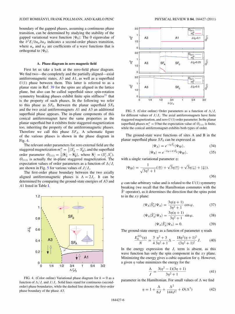
First let us take a look at the zero-field phase diagram.We find two—the completely and the partially aligned—axialantiferromagnetic states, A3 and A1, as well as a superfluidU (1) phase between them. This latter is referred to as aplanar state in Ref. 39 for the spins are aligned in the latticeplane, but also can be called superfluid since spin-rotationsymmetry breaking phases exhibit finite spin stiffness21 thatis the property of such phases. In the following we referto this phase as SF0. Between the planar superfluid SF0

and the two axial antiferromagnets A1 and A3 an additionalsuperfluid phase appears. The in-plane components of thisconical antiferromagnet have the same properties as theplanar superfluid but it exhibits finite staggered magnetizationtoo, inheriting the property of the antiferromagnetic phases.Therefore we call this phase SFA. A schematic figureof the various phases is shown in the phase diagram inFig. 4.

The relevant order parameters for zero external field are thestaggered magnetization mst

z = 12 |Sz

A − SzB |, and the superfluid

order parameter OU (1) = 12 |S⊥

A − S⊥B |, where S⊥

j = (Sxj ,S

y

j ).OU (1) is actually the in-plane staggered magnetization. Theexpectation values of order parameters as a function of �/Jz

are shown in Fig. 5 for various values of J/Jz.The first-order phase boundary between the two axially

aligned antiferromagnetic phases is � = 2Jz. It can bedetermined by comparing the ground-state energies of A3 andA1 listed in Table I.

0

A1

A3SF

SF

A

3/25/413/41/21/40

1.2

1

0.8

0.6

0.4

0.2

0

J/J z

Λ/ζJz

FIG. 4. (Color online) Variational phase diagram for h = 0 as afunction of �/Jz and J/Jz. Solid lines stand for continuous (second-order) phase boundaries, while the dashed line denotes the first-orderphase boundary of the phase A3.

mst z

OU

(1)

Λ/ζJ z

0

1/2

1

3/2

0 1/4 1/2 3/4 1 5/4 3/2

J/Jz=0.5

mst z

OU

(1)

0

1/2

1

3/2

J/Jz=0.25

mst z

OU

(1)

0

1/2

1

3/2

J/Jz=0.1

A3

A3

A3

SF

SF SF

A1

A 0

0

st

OU(1)

mstz

zmU(1)O

zstm

U(1)O

FIG. 5. (Color online) Order parameters as a function of �/Jz

for different values of J/Jz. The axial antiferromagnets have finitestaggered magnetization, and zero U (1) order parameter. In the planarsuperfluid phases mst

z = 0 but the expectation value of OU (1) is finite,while the conical antiferromagnet exhibits both types of order.

The ground-state wave functions of sites A and B in theplanar superfluid phase SF0 can be expressed as

|A〉 = e−iϕSzA |SF〉, (34)

|B〉 = e−i(ϕ+π)SzB |SF〉, (35)

with a single variational parameter η:

|SF〉 = 1√3η2 + 1

(|⇑〉 +√

3η|↑〉 +√

3η|↓〉 + |⇓〉).

(36)

ϕ can take arbitrary value and is related to the U (1) symmetrybreaking (we recall that the Hamiltonian commutes with theSz operator), as it determines the direction that the spins pointto in the xy plane:

〈A|SxA|A〉 = 3η(η + 1)

3η2 + 1cos ϕ, (37)

〈A|Sy

A|A〉 = 3η(η + 1)

3η2 + 1sin ϕ, (38)

〈A|SzA|A〉 = 0. (39)

The ground-state energy as a function of parameter η reads

ESF00 (η)

N= 3

4

η2 + 3

3η2 + 1� − 18η2(η + 1)2

(3η2 + 1)2J. (40)

In the energy expression the Jz term is absent, as thiswave function has only the spin component in the xy plane.Minimizing the energy gives a cubic equation for η. However,a given η value minimizes the energy for the

�

J= 3(η2 − 1)(3η + 1)

3η2 + 1(41)

parameter in the Hamiltonian. For small values of � we find

η = 1 + �

6J+ �2

144J 2+ O(�3) (42)

184427-6

SUPERSOLID PHASE AND MAGNETIZATION PLATEAUS . . . PHYSICAL REVIEW B 84, 184427 (2011)

and the ground-state energy can be approximated as

ESF00 = −9

2J + 3

4� − �2

16J+ O(�3), (43)

which gives the phase boundary with the antiferromagneticphase A3,

J = Jz − �

3− �2

72Jz

+ O(�3), (44)

as seen in Fig. 4.For � = 0, when the anisotropy is absent, η = 1 and

Eq. (36) is just a spin coherent state of the spin-3/2 Neelstate of the SU(2) symmetric Heisenberg model rotated intothe xy plane. For � > 0 the Sz = ±3/2 components in thewave function are suppressed. In the � → +∞ limit theη = �/3 + O(1) and we are left with a wave function withSz = ±1/2 spin components only. Out of these two states wecan mix a spin pointing to arbitrary direction; however thelength of the spin is not constant—it is the largest when lyingin the xy plane (the length is then 1 as opposed to 1/2 whenpointing in the z direction, a consequence that they are stillS = 3/2 spin). For this reason the antiferromagnetic exchangeterm gains the most energy with the planar spins, as in Eq. (36).When the exchange interaction becomes anisotropic, and theSz

i Szj term becomes strong, this energy can compensate the

directional length dependence of the spin and can choose aspin configuration with a finite z and xy component. Thishappens in the conical superfluid phase, denoted by SFA inFig. 4.

The phase boundary of the conical superfluid phase (SFA)toward the planar phase (SF0) and fully polarized AFM phase(A3) is a complicated expression. It is shown in Fig. 4.Starting from phase A1 at a given � value, a second-orderphase transition occurs to the superfluid phase SFA. Whenthe exchange coupling J is large enough, in-plane spincomponents appear continuously as we reach into SFA. Theground state can be expressed as follows:

|A〉 ∝ e−iϕSzA (|⇑〉 + u|↑〉 + v|↓〉 + w|⇓〉), (45)

|B〉 ∝ e−i(ϕ+π)SzB (w|⇑〉 + v|↑〉 + u|↓〉 + |⇓〉), (46)

with real u, v, and w variational parameters.The instability of the partially aligned AFM phase A1

against canting gives the phase boundary

J = Jz(Jz − �)

Jz − 4�(47)

between A1 and SFA.The same model for one dimension has been treated by

mean-field calculations in Ref. 39 for quantum spin 1/2, 1,

and 3/2. The phase diagram for the case S = 3/2 is similarto our findings; however the conical superfluid phase SFA ismissing due to a more restricted variational wave function theyused.

B. Heisenberg exchange with on-site anisotropy

In the following we discuss the phase diagram as thefunction of magnetic field and single-ion anisotropy when theexchange between two neighboring sites is SU(2) symmetric(i.e., the J = Jz Heisenberg model with on-site anisotropy).

h z

Λ/ζ

/ζJ

Jz

z

0

2

4

6

8

10

0 1 2 3 4 5

F1

SFF

F3

zJ=J

FIG. 6. (Color online) Phase diagram as a function of �/J andhz/J (Jz = J ).

The phase diagram outlined in Fig. 6 was calculated by thevariational method introduced above.

On the hz = 0 line the ground state is the planar superfluidphase (SF0) introduced previously. As the magnetic fieldbecomes finite, the spins cant out of the plane continuously, andthe superfluid ground state SFF exhibits finite magnetizationmz alongside the finite staggered in-plane order parameterOU (1) (Fig. 7). A schematic figure of the conical SFF isshown in Fig. 6 and the ground-state wave function can becharacterized as

|A〉 ∝ e−iϕSzA (|⇑〉 + u|↑〉 + v|↓〉 + w|⇓〉), (48)

|B〉 ∝ e−i(ϕ+π)SzB (|⇑〉 + u|↑〉 + v|↓〉 + w|⇓〉), (49)

where u, v, and w are all real numbers.The ground-state energies of the axial ferromagnetic phases

and the fully polarized ferromagnetic state are given in Table I.Analytical expression for the ground-state energy of SFF

is beyond our reach; however, the phase boundary with theneighboring F3 phase can be given by calculating the criticalfield for the polarized phase. This is exactly the same asthe instability approximation for F3 in the case of the Isinglimit, and is given by the same Eq. (21). Above the saturationfield the fully polarized ferromagnetic phase is stabilized. Forlarge enough values of � the spins become shorter and thepartially polarized plateau phase F1 emerges. Calculating theinstability of F1, the phase boundary turns out be

h = J + 2Jz + � ±√

J 2 − 14J� + �2. (50)

As expected, from the mapping to the effective XXZ model(Sec. II B), we found no evidence for gapped phases that breakthe translational symmetry.

C. The effect of exchange anisotropy and the emergence of thesupersolid phase

Finally let us examine the collective effect of exchange andsingle-ion anisotropies as well as the magnetic field. In theprevious subsection we learned that only the ferroaligned spins

184427-7

JUDIT ROMHANYI, FRANK POLLMANN, AND KARLO PENC PHYSICAL REVIEW B 84, 184427 (2011)

mz

OU

(1)

hz/ζJz

0

1/2

1

1/3

0 2 4 6 8 10

Λ/ζJz=9/2

mz

OU

(1)

0

1/2

1

1/3Λ/ζJz=3

mz

OU

(1)

0

1/2

1

1/3Λ/ζJz=3/2

mz

OU

(1)

mz

0

OU(1)

1/2

1

1/3Λ/ζJz=0

F

SFF

SF

SFF

F3

F3

F3

F

F1

SFF

SF

FIG. 7. (Color online) Order parameters as a function of magneticfield for different values of � parameter. The fully and partiallypolarized ferromagnets F3 and F1 exhibit finite magnetization mz,while in the conical ferromagnetic phase SFF the expectation valuesof both mz and OU (1) are finite.

in F1 and F3 are present as gapped phases for the case of theHeisenberg exchange (Jz = J ), with a superfluid phase (cantedantiferromagnet) in between them. As the value of J/Jz is low-ered, islands of plateaus and antiferromagnetic phases emergein the sea of the superfluid phase. We choose a relatively largeanisotropy J/Jz = 0.2, as in that case we learned from theperturbational expressions that the 2-fold degenerate gappedphases might be stable, as shown in Fig. 2(a). Indeed, thevariational phase diagram, shown in Fig. 2(b), displays all thephases we were looking for: The superfluid phase takes placearound the axial ferromagnets, while between the plateausand axial antiferromagnetic phases—i.e., the gapped phasesthat exhibit staggered diagonal magnetic order—a very robustsupersolid phase arises.

The extension of the supersolid around the phases A1 andP 2 is the broadest at their tips, when � is not too large. As weincrease �, the supersolid region decreases, and eventuallyvanishes for � → +∞. Since in this limit the mapping tothe XXZ model becomes exact (Sec. II B), our finding is alsoconsistent with numerical works on the XXZ model on thesquare lattice that do not seem to find the supersolid.13,37,38

The variational calculation finds all the phase boundariesto be of second order, except a single first-order one around� ≈ 2Jz [shown in dashed line in Fig. 2(b)] that is inheritedfrom the J = 0 phase diagram, Fig. 1.

The expression of the phase boundaries of the axial ferro-magnetic phases are the same as in the Heisenberg limit [seeEqs. (21) and (50)]. We determined the phase boundaries ofthe plateaus and axial antiferromagnetic states by calculatingspin wave instability. We found that the boundary for the 2/3plateau can be given as

� = h

2− � ±

√(� − 3Jz)2 − 9J 2, (51)

with � = 2Jz + 6J 2

h/2−3Jz. Similar calculations give

h =√

2(J 2

z − J 2) + 2(Jz − �)2 − 2�,

(52)� =

√[J 2 − �(� − 2Jz)]2 + 32J 2�(2� − Jz)

for the phase boundary of the partially polarized axialantiferromagnetic phase A1,

� = � − h

2±

√(� − 3Jz)2 − 9J 2 , (53)

with � = 2Jz + h2 + 6J 2

h/2−3Jz, for the phase boundary of P 1

plateau, and

� = 3Jz −√

h2

4+ 9J 2 (54)

for the boundary of the axial antiferromagnetic phase A3.When J = 0 Eq. (53) and (54) give back the h = 6Jz − 2�

phase boundary that separates A3 and P 1 in the Isinglimit. The ground-state energies and phase boundaries forthe superfluid and supersolid phases can only be obtainednumerically. The ground-state wave function for the superfluidwith ferromagnetic mz is given by Eq. (49), and for thesupersolid by

|A〉 ∝ e−iϕSzA (|⇑〉 + u|↑〉 + v|↓〉 + w|⇓〉), (55)

|B〉 ∝ e−i(ϕ+π)SzB (|⇑〉 + u′|↑〉 + v′|↓〉 + w′|⇓〉), (56)

where u, u′, v, v′, w, and w′ are all real. Figure 8 shows theevolution of the order parameters which can be used to findout the nature of the phases as we increase the magnetic fieldfor a few selected values of �/Jz.

D. S = 1 phase diagram

At this stage, it is useful to compare the predictions of thevariational approach to a better studied problem. Supersolidphases have been found in a spin-1 anisotropic Heisenbergantiferromagnet in Ref. 23, so we constructed the variationalphase diagram for this model as well. The Hamiltonian isidentical to Eq. (1), but now with S = 1 spin operators.The phase diagrams, for vanishing J and J = 0.2Jz, areshown in Fig. 9. In the Ising limit, Fig. 9(a), we find twouniform phases (denoted as 00 and 11, using the values ofthe Sz components) and two phases breaking the translationalsymmetry: the 11 with zero magnetization and the 10 one-halfmagnetization plateau. The XXZ-like physics can be identifiedfor the transition between the 11, 10, and 00 phases, where thesupersolidity is a fragile phase. The region between the 10 and11 is of a different nature, and we expect the supersolid to berobust in this part of the phase diagram. And that is exactlythe region where Ref. 23 found supersolidity. Furthermore, thenature of the phase transitions is also in qualitative agreement,inasmuch as the order of the phase transitions is concerned.Specifically, we recover the first-order transition between theupper boundary of the 10 phase and the superfluid. It is alsouseful to compare Fig. 9(b) to the phase diagram of theone-dimensional chain obtained by DMRG:29 The extent ofthe gapped phases is reduced in the chain, and the supersolidsurvived only in a small region close to the 11 phase.

184427-8

SUPERSOLID PHASE AND MAGNETIZATION PLATEAUS . . . PHYSICAL REVIEW B 84, 184427 (2011)

mst z

OU

(1)

hz ζ/ Jz

0

1/2

1

1/3

0 0.5 1 1.5 2 2.5

mz

mxy

0

1/2

mst z

OU

(1)

0

1/2

1

1/3

mz

mxy

0

1/2

1

1/3

Λ/ζ

Λ/ζ

J

Jz

z

=3/8

=9/8

mst z

OU

(1)

OU(1)

mstz

0

1/2

1

1/3

mz

mxy

mzmxy

0

1/2

1

1/3 Λ/Jz=0

P2

SS SF

A1

SS

SF F1 SF

SSA3

F3SF

P1

A3

SS

FIG. 8. (Color online) Expectation value of order parametersper site as a function of h/Jz for different values of �/Jz. Inthe axial antiferromagnetic phases A1 and A3 only the staggeredmagnetization has finite expectation value. For � = 0 there isa first-order phase transition from the completely polarized A3phase to the superfluid phase. All the other field-induced transitionsare second-order transitions. The superfluid phase exhibits finitemagnetization mz and finite staggered in-plane magnetization OU (1).The ferromagnetically ordered phases F3 and F1 are characterizedby finite magnetization mz, while the plateaus (P 1 and P 2) have anadditional finite staggered magnetization mst

z . In the supersolid phaseall four order parameters have finite expectation values.

The calculation of the phase diagram is quitestraightforward—assuming two-sublattice order, the varia-tional wave function is given by Eq. (31), now with

|ψA〉 ∝ u1|1〉 + eiξ0u0|0〉 + eiξ1u1|1〉 (57)

and a similar expression for |ψB〉. We are now dealing with8 independent variational parameters altogether, which canbe reduced to 7 by using the U (1) symmetry of the model.Similarly to the spin-3/2 case, we get solutions where allthe amplitudes can be chosen to be real numbers for theHamiltonian we look at.

The saturation field is given by hsat = � + ζJz + ζJ , andfrom the stability analysis of the 11, 00, and 10 gapped phaseswe get the following equations for their phase boundaries:

h2 = (ζJz − � − ζJ )(ζJz − � + ζJ ), (58)

h2 = �(� − 2ζJ ), (59)

(h − �)(ζJz + � − h)(h − ζJz + �) = 2ζ 2J 2�, (60)

respectively.

(a)

(b)

hz

/J

Λ/

z

Jz

zh J

ζ

ζ / z

1/2

1

1 3/4

3/2

0 1/4 1/2

3/2

1

0

0

1/2

3

NW2 2 N/2×

NW

11

SF

SS SF

00

11

11

11

10

00

10

FIG. 9. (Color online) The phase diagram of the anisotropic S =1 model in the (a) Ising limit for a bipartite lattice with coordinationnumber ζ and (b) for the square lattice (ζ = 4) when J = 0.2Jz,obtained from the variational calculation.

IV. SUPERSOLID IN THE ONE-DIMENSIONAL MODEL

In this section we complement the variational study usinga variant of the density matrix renormalization group40

(DMRG) method on the anisotropic S = 3/2 spin chain. Aquantum Monte Carlo study has shown that a supersolid phasecan realized in the anisotropic S = 1 spin chain,27 a resultconfirmed by DMRG calculations in Refs. 28–30. Thereforeit is plausible that a supersolid state is also present in theanisotropic spin-3/2 chain.

We map out the phase diagram for the chain and search forsignatures of supersolid phases. The DMRG method we usedoptimizes variationally a wave function based on a matrix-product state41 (MPS) ansatz for an infinite chain. Algorithmsusing this approach are efficient in one-dimensional systemsbecause they exploit the fact that the ground-state wavefunctions are only slightly entangled. For mapping out thephase diagram, we used comparably small matrix dimensions

184427-9

JUDIT ROMHANYI, FRANK POLLMANN, AND KARLO PENC PHYSICAL REVIEW B 84, 184427 (2011)

FIG. 10. (Color online) Zero-field phase diagram for the infinitechain as a function of �/Jz and J/Jz, as obtained from DMRG cal-culation with χ = 25. Panel (a) shows the staggered magnetization.Panel (b) shows the half-chain entanglement entropy, i.e., the vonNeumann entropy of the reduced density matrix for a bipartition ofthe chain into two half chains.

of χ = 50, while for estimating the central charge we usedmatrices up to χ = 200.

The zero magnetic field phase diagram is shown in Fig. 10.We can clearly identify the gapped A3 and A1 uniaxial phaseswith finite value of the staggered magnetization mst

z and smallentanglement entropy, and a gapless phase with algebraiccorrelations (Luttinger liquid). The extension of the A1 phaseis limited to J/Jz � 0.25 values, following the estimate basedon the mapping to the XXZ model in Sec. II B.

Figure 11 shows the phase diagram in the present finitemagnetic field. Again, the gapped phases can be identifiedusing the uniform and staggered magnetization (mz andmst

z ), and the small entanglement entropy. The extension ofthe gapped phases essentially follows the variational phasediagram [see Fig. 2(b)]. However, the supersolid phase is morefragile in the one-dimensional case due to strong quantumfluctuations. Consequently, the gapless phase in the phasediagram is predominantly a simple Luttinger liquid (LL) withalgebraically decaying correlations and characterized by theinteger central charge that measures the number of gaplessmodes. We calculated the central charge of the gapless phasesusing the method outlined in Ref. 42 for a few selected points inthe phase diagram. Within numerical accuracy we find c = 1,as shown in Fig. 12. This is in accordance with our expectationoriginating from the mapping to the effective XXZ model, thatthe gapless phases between the F3 and P 2, P 2 and F1, andF1 and A1 are all Luttinger liquids.

We have searched for a supersolid phase in the vicinityof the gapped phases that break the translational invariance.We made a scan by varying the field for a fixed value of�/Jz and J/Jz; the results are plotted in Fig. 13. For thesimulations, we added a tiny magnetic field of order 10−4

along the x axis to break the U(1) symmetry around the z axis.A finite value of the diagonal (staggered magnetization mst

z )and off-diagonal (magnetization along the x axis, mx) orderparameter indicates the presence of the supersolid. It appearsthat the supersolid is stable in a small region only, between theA3 and P 1 gapped phase, with a continuous phase transitions.

FIG. 11. (Color online) Phase diagram as a function of �/Jz andh/Jz for (a)–(c) J/Jz = 0.1 and (d)–(f) J/Jz = 0.2. We show theuniform and the staggered magnetization along the z axes, wherethe plateau phases can be identified. The large increase of theentanglement entropy indicates gapless phases. The phase diagram isobtained from DMRG calculation with χ = 25.

Both the magnetization and the staggered magnetization in thesupersolid show a square-root-like behavior at the lower andupper critical fields, like the magnetization in the XXZ modeldoes; see for example Ref. 43. This is due to the density ofthe states of the spinons, and is already observed in the XY

model, when it is mapped to free fermions. Recall that thedensity of states of free fermions has a van Hove singularity atthe band edges, and this shows up as a square root singularityin the magnetization curve of the XY (and XXZ) model. InFig. 14 we straighten out this singularity. This singularity isalso inherited for the staggered magnetization at the criticalfields. The central charge in the supersolid is also c = 1 (the

S

ln ξ

J/Jz=0.2

h=5,Λ=1h=3,Λ=1h=4,Λ=1.5h=0.5,Λ=1.5h=1.95,Λ=0.5 0.6

0.7

0.8

0.9

1

1.1

1.2

3 3.5 4 4.5 5 5.5

FIG. 12. (Color online) Estimate of the central charge from theentanglement entropy for four different points in the LL phase and onepoint in the supersolid phase (the h/Jz = 1.95, �/Jz = 0.5 point).The solid lines are fits based on the S = c

6 ln ξ + const. formula, withc set to 1. In all these points the gapless phases are characterized byc = 1 central charge.

184427-10

SUPERSOLID PHASE AND MAGNETIZATION PLATEAUS . . . PHYSICAL REVIEW B 84, 184427 (2011)m

st z

mx

hz/Jz

(b)

mstz

mx

2

2.5

3

1.7 1.8 1.9 2 2.1 2.2 0

0.1

0.2

0.3

0.4

0.5

mz

mst x

(a)

A3 SS P1

mzmst

x

0

0.5

1

0

0.2

0.4

0.6

0.8

FIG. 13. (Color online) The magnetic field dependence of theorder parameters as a function of the magnetic field for J/Jz = 0.2and �/Jz = 0.5. The curves are the result of DMRG calculations withχ = 40 and with a small field hx/Jz = 10−4. In (a), the nonvanishingoff-diagonal order parameter mst

x shows the extension of the gaplessphases. The finite value of the mst

z and mx indicate a robust supersolidphase, as seen in (b).

lowest line in Fig. 12; here we set the hx = 0, as otherwise afinite hx induces a gap in the spectrum).

From variational calculations, we expect a continuous phasetransition into the supersolid also at the upper edge of the P1

phase. Numerically, however, we find a first-order transitioninto the LL phase.

V. EXACT DIAGONALIZATION STUDIES

To get further insight into the problem in higher dimensions,we have numerically diagonalized small (8- and 10-site)clusters of spin S = 3/2 arranged on the square lattice withperiodic boundary condition and searched for the signature ofdifferent phases in the energy spectrum. The two-sublatticestates break translation symmetry, so we expect two degen-erate ground states with momentum k = (0,0) and (π,π ) inthe thermodynamic limit. In the gapped phases, these twolevels are well separated from the other states, while inthe supersolid, where both translational symmetry and U(1)symmetry breaking occurs, we expect two copies of theAnderson towers in the spectrum that is the signature of the

(mz)

2

hz/Jz

(a) 0

0.05

0.1

0.15

1.86 1.88 1.9

(1-m

z)2

hz/Jz

(b) 0

0.05

0.1

0.15

1.96 1.98 2 2.02

FIG. 14. (Color online) The magnetization has a square rootsingularity at (a) lower hc,1/Jz = 1.8579, and (b) upper hc,2/Jz =2.0195 critical field. The solid lines show the m2

z ≈ 2.68(h −hc,1)/Jz + 16.9(h − hc,1)2/J 2

z and (1 − mz)2 ≈ 1.27(hc,2 − h)/Jz +13.2(hc,2 − h)2/J 2

z fits to the magnetization curves.

2

0

−2

−4E/J

z

−6

−8

−10 2

0

−2

−4

−6

E/J

z

−8

−10 1.5 1.6 1.7 1.8 1.9 2 2.1 2.2 2.3

(a)

(b)

z

J = 0.2 JS = 1

S = 0z

z

z

(0,0)J = 0.2 J

(π,π)(3π/5,π/5)

(2π/5,4π/5)

(2π/5,4π/5)(3π/5,π/5)

(π,π)(0,0)

(π,π)

(0,0)

z/JΛ

FIG. 15. (Color online) The first few lowest lying energy levelsof a 10-site cluster for (a) Sz = 0 and (b) Sz = 1 as a function of�/Jz. We set J = 0.2Jz. The inset shows the available k points inthe Brillouin zone.

U (1) symmetry breaking.44,45 Unfortunately, the large spinmakes the finite-size scaling difficult, and without a finite-sizescaling we cannot be sure about the exact nature of the groundstate. Nevertheless, even our small cluster gives importantsupport for the variational phase diagram.

In Fig. 15 we show the energy spectrum for the C4

symmetric 10-site cluster and J = 0.2Jz around � = 2Jz,where we expect the first-order transition from the phase A3into the supersolid to happen. In zero field the ground statehas Sz = 0, and in Fig. 15(b) we see that the energy-levelcurvatures of lowest lying states in the k = (0,0) and (π,π )sector are essentially indistinguishable for � � 1.88Jz andwell separated from the higher levels. This indicates thepresence of a gapped, two-sublattice state that we can associate

FIG. 16. (Color online) The gap � = E(π,π ) − E(0,0) as a functionof �/Jz and h/Jz for the 10-site cluster. The solid curves separatethe different Sz sectors.

184427-11

JUDIT ROMHANYI, FRANK POLLMANN, AND KARLO PENC PHYSICAL REVIEW B 84, 184427 (2011)

mz

hz/hsat

MFED0

0.5

1

1.5

0 0.2 0.4 0.6 0.8 1

Λ/Jz=4.5

(c)

mz

MFED0

0.5

1

1.5

Λ/Jz=1.5

(b)

mz

MFED0

0.5

1

1.5

Λ/Jz=0

(a)

FIG. 17. (Color online) Magnetization as a function of magneticfield, as obtained from variational calculation and exact diagonaliza-tion. Here J = 0.2Jz, and �/Jz =0, 1.5, and 4.5. hsat is the saturationfield [Eq. (21)].

with the A3 phase. The sharp level anticrossing at � ≈ 1.88Jz

indicates a first-order transition. In the Sz = 1 sector we ob-serve the spin excitations with a narrow bandwidth and a k ↔(π,π ) − k symmetry, following Eq. (A16) as calculated fromthe perturbation theory in Sec. II E. For � � 1.88Jz, the k =(0,0) and (π,π ) levels are also close, and the these two levelsare equally close and reversed in order for Sz = 1 in Fig. 15(a),an indication for the U(1) symmetry breaking, possibly withtranslational symmetry breaking (the supersolid phase).

In Fig. 16 the energy gap between the k = (0,0) and (π,π )ground states in the different Sz sectors is shown as a functionof �/Jz and magnetic field, as this may serve as an indicatorof the translational symmetry breaking. We can identify thegapped phases (except for A1) and their extension is evenquantitatively in good agreement with the variational phasediagram, shown in Fig. 2(b). The consistency between thevariational and exact diagonalization result is also supportedin Fig. 17, where we compare the magnetization calculated bythese two methods.

VI. CONCLUSIONS

In this paper we studied the effect of exchange and easy-plane anisotropies on the formation of magnetization plateausand supersolids in spin-3/2 system on (unfrustrated) bipartitelattices, with the aim to extend the results of earlier studies onthe stability of supersolids in anisotropic spin-1 model on thesquare lattice23 and spin-1/2 bilayer systems22,24,25 to largervalues of spins.

In the Ising limit (J = 0) we find both uniform andtranslational symmetry breaking magnetic phases with gappedexcitation spectrum with zero finite magnetization (magneti-zation plateaus). We discussed the macroscopic degeneracyof the ground state at the phase boundaries and showed thatwhen the off-diagonal exchange interaction J becomes finite

this degeneracy is lifted and new gapless phases emerge. Allthe plateaus continuously evolve from the Ising limit, and thedegeneracy of the boundaries in the Ising limit gives a hint onthe order of the phase transition and on the nature of the gaplessstate. Not surprisingly, our variational calculation shows thatthe supersolid phases are concentrated around the plateaus thatbreak the translational symmetry. In particular, the tendencytoward supersolidity is greatly enhanced when the degeneracyof the boundary is 2 × 2N/2 (due to the choice of two stateson the sites of one of the sublattices, while the sites of theother sublattice are occupied with a third type of states), asin this case the diagonal translational order is preformed, andthe off-diagonal order is easily established on the sublatticeoccupied with the two states. In addition, for large anisotropieswe have confirmed the stability of the plateau states usingperturbation theory, and found a good agreement between thetwo approaches regarding the extension of the gapped phases.

In zero field we plotted the variational phase diagram as afunction of the on-site and exchange anisotropies. Aside fromthe axial antiferromagnetic phases and planar superfluid phase,we find a biconical superfluid which simultaneously exhibitsthe diagonal and off-diagonal staggered characteristics of theformer phases.

In the J = Jz Heisenberg limit, when the exchange inter-action is SU(2) invariant [but we keep the on-site anisotropy� that breaks the SU(2) symmetry], the plateau and supersolidphases disappear and only the uniform phases and thesuperfluid phase between them are present.

The variational phase diagrams for zero and finite magneticfield were compared to DMRG calculations carried out inone dimension. We have found convincing evidence for asupersolid state that is realized in a region between twogapped phases that break the translational symmetry. For atwo-dimensional square lattice, we performed exact diagonal-ization on small clusters for J/Jz = 0.2 and identified thecharacteristics of various phases from the energy spectrum.The extension of the gapped phases based on these calculationsproved to be in good qualitative and quantitative agreementwith the variational findings.

Our study was initially inspired by the Ba2CoGe2O7 layeredmaterial, where Ref. 35 estimates �/Jz ≈ 8 and J ≈ Jz. Whilethese anisotropies are not strong enough to stabilize a magne-tization plateau, an anomaly occurs around m/msat = 1/3 inthe magnetization curve. This is also observed experimentally:The magnetization curve changes its slope at h ≈ 9 T, as seenin Fig. 3(b) in Ref. 34.

ACKNOWLEDGMENTS

We are pleased to acknowledge stimulating discussionswith S. Bordacs, I. Kezsmarki, L. Seabra, and P. Sindzingre.We are also grateful to H. Murakawa for sharing his magne-tization measurements with us. This work was supported byHungarian OTKA Grant Nos. K73455 and NN76727, and theguest program of MPI Physik Komplexer Systeme in Dresden.

APPENDIX: PERTURBATION EXPANSION

Here we are presenting the results of the Rayleigh-Scrodinger perturbation theory applied to states and excitationsin the J → 0 limit.

184427-12

SUPERSOLID PHASE AND MAGNETIZATION PLATEAUS . . . PHYSICAL REVIEW B 84, 184427 (2011)

1. Second-order corrections in J to the ground-state energy

The second-order corrections to the energy (per site) of thedifferent phases are as follows:

ε(2)A1 = −8J 2

3Jz

− 9J 2

2(4� − 5Jz), (A1)

ε(2)A3 = − 9J 2

2(11Jz − 4�), (A2)

ε(2)F1 = − 12J 2

2� − Jz

, (A3)

ε(2)P 1 = − 6J 2

7Jz − 2�, (A4)

ε(2)P 2 = −3J 2

2Jz

, (A5)

ε(2)F3 = 0. (A6)

2. First-order degenerate perturbation theory for excitationspectrum of the uniform F1 and F2 phases

ωF1→P 2 = −h + 2Jz + 2� + 6Jγk, (A7)

ωF1→A1 = h − 2Jz + 8Jγk, (A8)

ωF3→P 2 = h − 6Jz − 2� + 6Jγk, (A9)

where γk is defined in Eq. (18).

3. Second-order degenerate perturbation theory for excitationspectrum of the staggered phases

ωP 1→A3 = h + 2� − 6Jz − 36J 2

8Jz − 2�

− 9J 2

4(8Jz − 4�)16γ 2

k + 48J 2

7Jz − 2�, (A10)

ωP 1→P 2 = −h + 6Jz − 3J 2

2Jz

+ 48J 2

7Jz − 2�

− 3J 2

6Jz − 2�

(16γ 2

k + 8), (A11)

ωA1→F1 = −h + 2Jz − 27J 2

4� − 4Jz

− 12J 2

2� − 2Jz

+64J 2

3Jz

+ 36J 2

4� − 5Jz

− 2J 2

Jz

(16γ 2

k + 8)

− 3J 2

2� − 4Jz

16γ 2k , (A12)

ωP 2→F3 = −h + 6Jz + 2� − 9J 2

8Jz

(16γ 2

k + 8) + 12

J 2

Jz

,

(A13)

ωP 2→F1 = h − 2Jz − 2� − 12J 2

2Jz + 2�− 9J 2

8Jz

16γ 2k

− 3J 2

2� − 4Jz

16γ 2k + 3J 2

Jz

, (A14)

ωP 2→P 1 = h − 6Jz + 21J 2

4Jz

− 3J 2

4Jz − 2�16γ 2

k , (A15)

ωA3→P 1 = −h + 6Jz − 2� − 12J 2

10Jz − 2�+ 36J 2

11Jz − 4�

− 9J 2

8(5Jz − 2�)

(16γ 2

k + 8). (A16)

In the case for which we include the excitations on bothsublattices, the S−

i excitations from the A1 in the k spaceare eigenvalues of the

HA1 =(

2Jz − h − 2J 2

Jz

(16γ 2

k + 8) − 27J 2

4�−4Jz− 12J 2

2�−2Jz4√

3Jγk

4√

3Jγk 2� − 2Jz − h − 12J 2

Jz− 9J 2

4(4�−6Jz)

(16γ 2

k + 8))

− 8ε(2)A1 (A17)

matrix. If we expand for J up to second order, this will give Eq. (A12), the corrections to the dispersion directly to the F1 phase.Similarly, for the P1 phase

HP 1 =(

2� + h − 6Jz − 36J 2

8Jz−2�6Jγk

6Jγk 2Jz + h − 2� − 8J 2

3Jz− 3J 2

6Jz−2�

(16γ 2

k + 8))

− 8ε(2)P 1, (A18)

and for the P2 phase

HP 2 =(

−6Jz + h − 27J 2

4Jz4√

3Jγk

4√

3Jγk −2Jz + h − 2� − 12J 2

2Jz+2�− 9J 2

8Jz

(16γ 2

k + 8))

− 8ε(2)P 2. (A19)

1C. N. Yang, Rev. Mod. Phys. 34, 694 (1962).2G. V. Chester, Phys. Rev. A 2, 256 (1970).3A. J. Leggett, Phys. Rev. Lett. 25, 1543 (1970).

4A. F. Andreev and I. M. Lifshitz, Sov. Phys. Usp. 13, 670 (1971).5E. Kim and M. H. W. Chan, Nature (London) 427, 225 (2004).6A. S. C. Rittner and J. D. Reppy, Phys. Rev. Lett. 97, 165301 (2006).

184427-13

JUDIT ROMHANYI, FRANK POLLMANN, AND KARLO PENC PHYSICAL REVIEW B 84, 184427 (2011)

7M. Kondo, S. Takada, Y. Shibayama, and K. Shirahama, J. LowTemp. Phys. 148, 695 (2007).

8Y. Aoki, J. C. Graves, and H. Kojima, Phys. Rev. Lett. 99, 015301(2007).

9T. Leggett, Science 305, 1921 (2004).10P. W. Anderson, Nature Phys. 3, 160 (2007).11P. W. Anderson, Phys. Rev. Lett. 100, 215301 (2008).12P. W. Anderson, Science 324, 631 (2009).13G. G. Batrouni and R. T. Scalettar, Phys. Rev. Lett. 84, 1599 (2000).14P. Sengupta, L. P. Pryadko, F. Alet, M. Troyer, and G. Schmid, Phys.

Rev. Lett. 94, 207202 (2005).15K. Yamamoto, S. Todo, and S. Miyashita, Phys. Rev. B 79, 094503

(2009).16H. Matsuda and T. Tsuneto, Prog. Theor. Phys. Suppl. 46, 411

(1970).17K.-S. Liu and M. E. Fisher, J. Low Temp. Phys. 10, 655 (1973).18S. Wessel and M. Troyer, Phys. Rev. Lett. 95, 127205 (2005).19R. G. Melko, A. Paramekanti, A. A. Burkov, A. Vishwanath, D. N.

Sheng, and L. Balents, Phys. Rev. Lett. 95, 127207 (2005).20D. Heidarian and K. Damle, Phys. Rev. Lett. 95, 127206 (2005).21L. Seabra and N. Shannon, Phys. Rev. B 83, 134412 (2011).22K.-K. Ng and T. K. Lee, Phys. Rev. Lett. 97, 127204 (2006).23P. Sengupta and C. D. Batista, Phys. Rev. Lett. 98, 227201 (2007).24N. Laflorencie and F. Mila, Phys. Rev. Lett. 99, 027202 (2007).25J.-D. Picon, A. F. Albuquerque, K. P. Schmidt, N. Laflorencie,

M. Troyer, and F. Mila, Phys. Rev. B 78, 184418 (2008).26K. P. Schmidt, J. Dorier, A. M. Lauchli, and F. Mila, Phys. Rev.

Lett. 100, 090401 (2008).27P. Sengupta and C. D. Batista, Phys. Rev. Lett. 99, 217205 (2007).

28D. Peters, I. P. McCulloch, and W. Selke, Phys. Rev. B 79, 132406(2009).

29D. Peters, I. P. McCulloch, and W. Selke, J. Phys. Conf. Ser. 200,022046 (2010).

30D. Rossini, V. Giovannetti, and R. Fazio, Phys. Rev. B 83, 140411(2011).

31H. T. Ueda and K. Totsuka, Phys. Rev. B 81, 054442 (2010).32A. Zheludev, T. Sato, T. Masuda, K. Uchinokura, G. Shirane, and

B. Roessli, Phys. Rev. B 68, 024428 (2003).33H. T. Yi, Y. J. Choi, S. Lee, and S.-W. Cheong, Appl. Phys. Lett.

92, 212904 (2008).34H. Murakawa, Y. Onose, S. Miyahara, N. Furukawa, and Y. Tokura,

Phys. Rev. Lett. 105, 137202 (2010).35S. Miyahara and N. Furukawa, J. Phys. Soc. Jpn. 80, 073708 (2011).36A. Feiguin, S. Trebst, A. W. W. Ludwig, M. Troyer, A. Kitaev,

Z. Wang, and M. H. Freedman, Phys. Rev. Lett. 98, 160409 (2007).37M. Kohno and M. Takahashi, Phys. Rev. B 56, 3212 (1997).38S. Yunoki, Phys. Rev. B 65, 092402 (2002).39J. Solyom and T. A. L. Ziman, Phys. Rev. B 30, 3980 (1984).40S. R. White, Phys. Rev. Lett. 69, 2863 (1992).41S. Ostlund and S. Rommer, Phys. Rev. Lett. 75, 3537 (1995).42F. Pollmann, S. Mukerjee, A. M. Turner, and J. E. Moore, Phys.

Rev. Lett. 102, 255701 (2009).43M. Klanjsek, H. Mayaffre, C. Berthier, M. Horvatic, B. Chiari,

O. Piovesana, P. Bouillot, C. Kollath, E. Orignac, R. Citro, andT. Giamarchi, Phys. Rev. Lett. 101, 137207 (2008).

44P. W. Anderson, Phys. Rev. 86, 694 (1952).45B. Bernu, C. Lhuillier, and L. Pierre, Phys. Rev. Lett. 69, 2590

(1992).

184427-14