Heincke RV Cruise Report HE-301 Oceanographic and …epic.awi.de/37139/1/HE301.pdf · Oceanographic...
106
Alfred Wegener Institute for Polar Research Jacobs University Bremen Heincke RV Cruise Report HE-301 Oceanographic and Marine Geophysical Excursion, Bremerhaven - Helgoland Leg 1: 13.04.2009 - 15.04.2009 All cruise participants here 11.09.2009 Chief Scientists: Prof. J. Bijma, Prof. V. Unnithan & Prof. L. Thomsen
Transcript of Heincke RV Cruise Report HE-301 Oceanographic and …epic.awi.de/37139/1/HE301.pdf · Oceanographic...

Alfred Wegener Institute for Polar Research Jacobs University Bremen
Heincke RV
Cruise Report HE-301
Oceanographic and Marine Geophysical Excursion,
Bremerhaven - Helgoland
Leg 1: 13.04.2009 - 15.04.2009
All cruise participants here
11.09.2009
Chief Scientists: Prof. J. Bijma, Prof. V. Unnithan &
Prof. L. Thomsen

Report compiled by Vikram Unnithan ([email protected])
This is an educational excursion and forms part of the regular cirriculum atJacobs University Bremen. Students from the ESSRES PhD Research Schoolwill join in Legs I & II. Use of data and results needs the explicit permission of
the chief scientist and contributing students.Printed at Jacobs University Bremen,

Contents 11.09.2009
Contents
Heincke Cruise Report, 2009 i

11.09.2009 List of Figures
List of Figures
ii Heincke Cruise Report, 2009

List of Tables 11.09.2009
List of Tables
Heincke Cruise Report, 2009 iii
11.09.2009 List of Tables
Cruise Participants
2.1 Shipboard Scientific Party
iv Heincke Cruise Report, 2009

List of Tables 11.09.2009
Name Affiliation Contact Details
Vikram Unnithan Jacobs University [email protected] Bijma Jacobs University /
Albert Benthien AWIFlorian Neu Jacobs university [email protected] RichterUlrike RichterGert RohardSara GadebergIshan Basyal Jacobs University [email protected] Fischer Jacobs University [email protected] Gmez Betanzos Jacobs University [email protected] Iliev Jacobs University [email protected] Jain Jacobs University [email protected] Joshi Jacobs University [email protected] Merschel Jacobs University [email protected] Ovanesov Jacobs University [email protected] Pabortsava Jacobs University [email protected] Parks Jacobs University [email protected] Bora AWI [email protected] Hoffmann AWI [email protected] Ihrig AWI [email protected] Kersten AWI [email protected] Nehring AWI [email protected] Lindeque AWI [email protected] Pfeiffer AWI [email protected] Ridder AWI [email protected] SchwegmannAxinja Stark AWI [email protected] Tong AWI [email protected] Wiebe AWI [email protected] Wieters AWI [email protected] Blum ESSReS [email protected] Sadeghi ESSReS [email protected] Owonibi ESSReS [email protected] Hilboll ESSReS [email protected] Juba ESSReS [email protected] Stepanek POLMARJain Ren POLMAR
Table 0.1:
Heincke Cruise Report, 2009 v

11.09.2009 List of Tables
2.2. Crew List RV HEINCKE
Name Function
Robert Voss KaptainNils Tonnies 1st officerRemo Franke 2nd officerJurgen Szymanski Chief EngineerAbu Hackman ElectricianHorst Habecker CookDirk Gatjen BoatswainGunther Lewin BoatswainJose marujo ABBernhard Pruchnow SMKurt Siefert ABBruno Amaral AB
Table 0.2:
vi Heincke Cruise Report, 2009

11.09.2009
1 Objectives
by Jelle Bijma & Vikram Unnithan
1.1 Education
1.2 Scientific Research
Heincke Cruise Report, 2009 vii

11.09.2009
2 Cruise Narrative
by Maitri Fischer
Important - All times are UTC time (Local time -2h).
Day1 - April, 13th 2009
Heincke Cruise Report, 2009 1

11.09.2009 2 Cruise Narrative
Time Event Location (Degrees) Equipment
5:00 Echosounder turned on Bremerhafen PortPre 8:00 Arrival of all participants. Ja-
cobs students, AWI students,ERASMUS students and in-structors. Loading of equipt-ment and food stuff.
Bremerhafen Port
8:00 the RV Heincke left port,heading for first destination
Bremerhafen Port
9:00 Jacobs Undergraduate stu-dent tasks handed out atrandom.
12:47 Arrive at Way pt. 1. Beginingof line (BoL) for Multibeam.
lon=7.758, lat= 53.998 Multibeam
13:12 Arrive at way pt2. End of line(EoL) for Multibeam.
lon =7.758, lat=54.048 Multibeam
13:17 BoL for the multibeam. lon =7.758, lat=54.048 Multibeam13:40 Arrive at way pt 3. EoL for
the multibeam.lon =7.757, lat=53.997 Multibeam
13:57 Deployment of CTD Way pt 3 CTD14:20 Deployment of Micro Sedi-
ment CorerWay pt 3 Micro Sedi-
ment Corer14:25 leave to way pt 4 Way pt. 315:04 BoL for the multibeam. lon =7.783, lat=54.042 Multibeam15:08 Begining of magnetics read-
ing. Milen Iliev, Vikram Un-nithan and a driver on asmall rubber boat towed themagnetometer.
lon= 7.782, lat=54.04 Magnetometer
15:11 The sidescan was deployedand BoL for the sidescan.
lon= 7.013, lat= 54.001 Sidescansonar
16:34 EoL for the multibeam. lon =8.064, lat=54.068 Multibeam16:51 EoL for the Sidescan lon= 8.002, lat= 54.001 Sidescan
Sonar16:52 Way pt 5 reached and EoL for
magnetics measurement.lon=8.115, lat=54.073 Magnetometer
17:11 BoL for Multibeam. lon=8.084, lat=54.070 Multibeam18: 55 EoL for Multibeam, and
RV Heincke docked in Hel-goland.
lon=7.894, lat=54.173 Multibeam
Table 2.1: Day 1, 13.April.2009
2 Heincke Cruise Report, 2009

11.09.2009
Day2 - April, 14th 2009
Heincke Cruise Report, 2009 3

11.09.2009 2 Cruise Narrative
Time Event Location (Degrees) Equipment
5:00 Echosounder turned on Helgoland port Echosounder6:05 RV Heincked left port Hel-
goland heading to Way pt 1.6:11 BoL for the Multibeam (just
some small runs befor thefirst way pt is reached)
lon=7.898 lat=54.176 Multibeam
6:29 Sidescan was started (BoL) lon= 7.015, lat=54.002 Sidescan6:27 EoL for Multibeam and BoL
for Multibeam Profile 9.lon=7.893, lat=54.141 Multibeam
6:33 Way point 1 was reached.Stop of Multibeam profile 9(EoL). BoL for new Multi-beam, profile 10.
lon= 8.065, lat=54.267 Multibeam
6:49 Arrive at Way pt 2. Endof Sidescan line (EoL) andmultibeam, and BoL forMultibeam (profile 11).
lon=7.014 , lat=54.003 Sidescan,Multibeam
7:04 Arrive at Way pt 3. CTDdeployed and EoL for Multi-beam.
lon=7.836 , lat=54.154 CTD, Multi-beam
7:20 Deployment of PlanktonMultinet.
Way pt 3 PlanktonMultinet
7:33 Arrive at Way pt 4. BoL forMultibeam, profile 13. BoLfor Sidescan (line 3).
lon=7.014 , lat=54.002 Multibeam,Sidescan
8:17 EoL for Sidescan (line 3) andEoL for Multibeam
lon=7.739◦ , lat=54.151◦ Sidescan
8:18 BoL for Sidescan (line 4) lon=7.012 , lat=54.003 Sidescan8:22 Arrive at Way pt 5. BoL for
Multibeam (profile 14)lon=7.738 , lat=54.150 Multibeam
8:34 Arrive at way pt 6. EoL forsidescan and Multibeam.
lon=7.7390 , lat=54.132 Sidescan,Multibeam
09:46 EoL for Multibeam (line 15)and BoL for Multibeam line16.
lon= 7.739, lat=54.132 Multibeam
09:47 BoL number 2 of magnetics. lon= 7.737, lat=54.132 Magnetometer10:57 EoL 2 of magnetics and
Multibeam.lon= 7.957, lat=54.133 Magnetometer,
Multibeam11:15 Arrive at Way pt 9. BoL for
multibeam.lon=7.964, lat= 54.131 Multibeam
12:52 Arrive at Way pt 10. EoL forMultibeam (line 17) and EoLfor Sidescan.
lon= 7.961, lat=54.245 Multibeam
Table 2.2: Day 2, 14.April.20094 Heincke Cruise Report, 2009

11.09.2009
12:53 BoL for Sidescan and BoL forMultibeam
lon= 7.961 lat= 54.245 Sidescanand multi-beam
12:59 EoL for sidescan and BoL forsidescan. EoL for Multibeam,and BoL for multibeam line19.
lon= 7.963, lat=54.245 Multibeam,Sidescan
13:34 EoL for sidescan and multi-beam.
lon= 895, lat=54.245 multibeam,Sidescan
13:35 Arrive at way pt 10. Be-gining of grid manover formultibeam and sidescan. Re-fer to Profile number 20 -25 from Multibeam measure-ments table and line 12-22for Sidescan in the sidescanmeasurements table.
lon=7.876, lat= 54.247 Multibeam,Sidescan
14:40 End of Grid manover formultibeam and sidescan.
lon=7.885, lat=54.258 Multibeam,Sidescan
14:40 BoL for multibeam (profile26)
lon=7.885, lat=54.258 Multibeam
15:03 EoL for multibeam lon=7.820, lat= 54.248 Multibeam15:04 BoL for multibeam (profile
27)lon=7.818, lat=54.247 Multibeam
15:10 EoL for multibeam lon=7.800, lat= 54.258 Multibeam15:11 BoL for multibeam (profile
28)lon=7.799, lat= 54.245 Multibeam
15:15 Deployment of CTD lon=7.798, lat=54.245 CTD15:25 Sediment boxcore deployed lon=7.798, lat=54.245 Boxcore16:05 EoL for multibeam profile 28 lon=7.898, lat=554.171 Multibeam16:15 RV Heincke Docked in Hel-
goland.Port Helgoland
Table 2.3: Continuation of table 2.2
Heincke Cruise Report, 2009 5
11.09.2009 2 Cruise Narrative
Main Equiptment on Board
• CTD
• sediment boxcore
• sediment microcore
• plankton multinet
• magnetometer
• sidescan sonar
• multibeam
• navigation hardware
• Simrad Echo-sounder
• Fisheries Echo-sounder
Some Pictures of the Equipment
Figure 2.1: Boxcore
6 Heincke Cruise Report, 2009
11.09.2009
Figure 2.2: CTD
Figure 2.3: Side Scan Sonar
Figure 2.4: Magnetometer
Heincke Cruise Report, 2009 7

11.09.2009 2 Cruise Narrative
Figure 2.5: Plankton Multinet
Figure 2.6: Sediment Micro-core
8 Heincke Cruise Report, 2009

11.09.2009
3 Navigation
3.0.1 DESCRIPTION OF INSTRUMENTS
As the navigation team on board, we were mostly involved with keeping a recordof the path of the vessel during the cruise. The Differential Global PositioningSystem (DGPS) was the main navigation system used on the Heinke researchvessel. In this section we analyse the theory of GPS, DGPS and GarMin.
• Global Positioning System (GPS)GPS is a global navigation satellite system. It uses a constellation of be-tween 24 and 32 medium Earth orbit satellites that transmit precise ra-diowave signals, which allow GPS receivers to determine the current lo-cation, time, and the velocity of a certain body on Earth. GPS is widelyused for navigation, map-making, land surveying, commerse, scientificuse, tracking, surveillance, etc. The work of a GPS device is based onreceiver that calculates its position by precisely timing the signals sent bythe GPS satellites high above the Earth. Each satellite continually trans-mits messages containing the time the message was sent, precise orbitalinformation, and the general system health and rough orbits of all GPSsatellites. The receiver measures the transmit time of each message andcomputes the distance to each satellites to determine the receiver’s loca-tion. The position is displayed, perhabs with a moving map display orlattitude and longitude; elevation information may be included (for exam-ple, on the OLEX operating system, if was possible to switch on and offthe elevation indicator). Many GPS units also show derived informationsuch as direction and speed, calculated from position changes.([?]). Onboard the Heincke, we used one GPS terminal that transfered informationof position and time to different softwares.This enabled the precise track-ing of the ship at every point of time.
• Differential Global Positioning System (DGPS)DGPS is an enhancement to GPS that uses a network of fixed, groundbased reference stations to broadcast the difference between the positionsindicated by the satellite systems and the known fixed positions. DGPSis used on ships, as was used on the Heincke. Its operation is based
Heincke Cruise Report, 2009 9

11.09.2009 3 Navigation
on a reference station that calculates differential corrections for its ownlocation and time. Users may be up to 200 nautical miles from the station,however, some of the compensated errors vary with space: specifically,satellite ephemeris errors and those introduced by ionospheric distortions.For this reason, the accuracy of the DGPS decreases with distance fromthe reference station.([?])
• GarMinGarMin is named after inventors Gary Burnell and Min Kao. Garmin isanother GPS hand-held device that is used, for instance, when Magne-tometry measurements are conducted. All current GarMin devices candisplay the current location on a map. The maps are vector based andstored in the buit in memory or loaded additional flash media. The buitin, so called ’basemap’, displays all country boarders and major cities. Onthe Heincke, GarMin was used on the dinghy send out for Magnetometry.This enabled us to get the precise position of the magnetometer as thedinghy trailed behind the vessel by about 200m. ([?])
————
3.0.2 METHODS OF DATA COLLECTION
As discussed in the previous section, data was obtained on the Heincke thoughDGPS. This data is received on softwares in the form of NMEA strings sent tothe data aquisition systems on board. In this section, we discuss the methodsof data collection by the DGPS.
• National Marine Electronic Association Strings (NMEA Strings)NMEA is a combined electrical and data specification for communicationbetween marine electronic devices. GPS receiver communication is de-fined within this specification. Most computer programs that provide realtime position information understand and expect data to be in NMEA for-mat.This data includes the complete PVT (position, velocity, time) solutioncomputed by the GPS receiver. The idea of NMEA is to send a line of datacalled sentence ot string that is totally self contained and independentfrom other sentences (strings). There are standard strings for each de-vice category and there is also the ability to define proprietary sentencesfrom use by individual company. All of the standard sentences have twolwtter prefix that defines the device that uses that sentence type.For GPSreceivers the prefix is GP, which followed by a three letter sequence thatdefines the sentence content.([?]) There are many sentences in the NMEAstandard for all kinds of devices that may be used in the Marine environ-ment. Some of the ones that have applicability to GPS receivers are listed
10 Heincke Cruise Report, 2009

11.09.2009
below as an example:([?])
GGA: time position, and fix data type.
GLL: lattiude, longitude, UTC time of position fix and status.
GSA: GPS receiver operating mode, satellites used in the position sulution, andDOP values.
GSV: The number of GPS satellites in view satellite, ID numbers, elevation,azimuth, and SNR values.
MSS: Signal-to-noise ratio, signal strength, frequency, and bit rate from aradio-beacon receicer.
RMC: Time, date, position, course and speed data.
VTG: Course and speed information relative to the ground.
ZDA PPS timing message (synchronized to PPS).
• Data Aquisition and Distribution (DATADIS)DATADIS was the data acquisition system on board the Heincke. It isa software designed for continuous recording of nautical, meteorological,survey, fishery and ship’s data and their digital and/or graphical process-ing, recording and storage. Data is strored as a daily file for at least 4weeks in addition on the SYSTEM-PS and can be used by the SYSTEM-PSand via Ethernet LAN (e.g. Challenger was used on board the Heincketo store and acquire data by all sceintists on board. The same server isnow accessible with the detailed records of all experiments conducted andnavigation data.) by any USER-PC for longterm graphic displays and in-dividual Voyage Recorder. All display, print and storage formats can becreated or changed by the client without any programming knowledge,using ’Drag and Drop’ method.([?])
————————————
3.0.3 DATA PROCESSING TECHNIQUES
As describes above, data is obtained onto the system in the form of NMEAstrings from the GPS or to the data acquisition system of Heincke DATADIS.The processing of data for the Navigation team involves making the data read-able by different softwares. The necessary coloumns of data, such as the co-ordinates, windstrength etc from the NMEA strings, for example, are separatedinto different files such that they can be used differently by different software
Heincke Cruise Report, 2009 11

11.09.2009 3 Navigation
such as ArcGIS or GMT. The processed data is then used on board on theOLEX system to keep a continuous track of the vessel’s movements. At anypoint of time, the ships velocity, water depth, direction, windspeed etc can bedetermined with this data.
The Navigation team focusses mostly on the navigation coordinates, i.e latitudeand longitude data but keeps a record of all other data obtained on thr GPSsince it is required by the scientists conducting the other experiments. Coor-dinates are obtained on the GPS in the digree- minute format and need to befirst converted into the readable decimal-degree format. This is done using thecomand ”awk” in the UNIX terminal. For example, the command-
awk ’{print int($1/100)+(($1-100*int($1/100))/60),int($2/100)+(($2-100*int100))/60)}’ file1.tex > file2.tex
will convert the necessary coloumns into the decimal-degree format and trans-fer the data from file1 to file2. This processed data can now, for example, beused by us in plotting the events on the cruise on a map. The experimentsconducted on board are broadly divided into two categories- point experiments,conducted while the vessel was stationery and track experiments, conductedalong a certain curise track. For each kind of experiment, the navigation teamskeep a record of the coordinates of the location of the vessel at the begin andthe end of the experiment and the exact time the experiment was conducted at.The following section has the required detailed plots, plotted on GMT.
12 Heincke Cruise Report, 2009

11.09.2009
3.0.4 RESULTS AND ANALYSIS
Using the techniques described above we created detailed plots and maps of allthe scientific experiments conducted on Heincke. With each experiment, detailssuch as the time, coordinates, depth, windstrength and speed were recordedby the DGPS. The navigation softwares on board were constantly updated bythe received data as the ship moved. The following maps were made usingGMT (Generic Mapping Tools: a software for the plotting and manipulation ofcartesian data sets) and ArcGIS (An ESRI developed Geographic InformationSystem). Different plots were created for different measurements to ensure theclarity of activities conducted on board. The caption on each map describes themethod being recorded. In the section after that, we discuss the shortcomingsof GPS and the possible errors in the data plotted.
Heincke Cruise Report, 2009 13
11.09.2009 3 Navigation
Figure 3.1: General Map of the Heinke cruise, 13-15 April 2009. The mapshows the route taken from Bremerhaven in North-West Germanyto the island of Helgoland. Bathymetry data is included in the back-groud since this data was used in addition to maps of the seafloorto determine the Way Points in the route of the cruise. Regionswith varying bathymetry were chosen and the vessel was made tomove over regions where known shipwrecks were lying. Often dur-ing the cruise, the course of the vessel had to be altered to suit theexperiments being conducted.
14 Heincke Cruise Report, 2009

11.09.2009
Figure 3.2: CTD measurements were made when the vessel was stationery. TheCTD was released into the water at three points during the cruiseto make conductivity, depth and temperature measurements. Thepoints and times of the CTD are located on this map.
Heincke Cruise Report, 2009 15

11.09.2009 3 Navigation
Figure 3.3: Multibeam measurements were made on board for certain sectionson the cruise track. These sections are marked on the map withthe start and end time for each section being indicated. The choiceof the cruise course reflects the locations of known shipwrecks andother bathymetric variances.
16 Heincke Cruise Report, 2009

11.09.2009
Figure 3.4: Side-scan measurements were made by the sidescan instrumentthat was released into the water and towed behind the ship at acertain distance. Care needed to be taken that a certain speedon the ship was maintained such that the sidescane does not trailalong the seabed. Also, notice the loops made on the path of thevessel before the end of the measurements. This is done on purposeso as to prevent the tangling of the sidescan instrument wires whilethe ship changed direction (and to prevent interference with theMagnetometry recordings) and to maintain the speed of the vessel.
Heincke Cruise Report, 2009 17

11.09.2009 3 Navigation
We note a few significant points from the data plotted above, such that theaccuracy of the cruise track may not be entirely correct sometimes, since manymeasuments are plotted to be at a slight distance from the determined cruisetrack. Also, the vessel’s GPS records different coordinates of location during thetime when the vessel is assumed to be stationery. This error could be resultof the movement of the vessel by the waves in the ocean, but at certain points,the error is significantly large such that corrections in the recorded coordinatesneeded to be made before plotting the maps. Though the coordinates providea reliable output when represented on the map, it is important to discuss theerror sources of GPS, as done in the proceeding section.
3.0.5 DISCUSSION OF LOGGED DATA AND CONCLUSIONS
From the Results and Analysis section we notice that the data measured bythe DGPS on board the Heincke is very precise, but has errors arising due toits inaccuracy at certain places. The coordinates recorded were good indicatorsof the vessels location on the map but the errors are more easily noticeablewhen different coordinate points were recorded during the time the vessel wasassumed to be stationery. Also, some of the recorded coordinates for the exper-iments were completely off the cruise track and had to be corrected manually toset them to the right locations. In this section we analyse the reasons for theseerrors and assess whether the final data obtained is reliable for the navigationteam or not.
Some of the possible errors of GPS include selective availability which meansthat, first, civil GPS receivers position determination is less accurate and fluc-tuates about 50 meters error. This problem however is slightly rectified becauseHeincke uses DGPS, but the errors in the locations are still noticible. Also, toindicate correct satellite geometry certain DOP values in the NMEA sentance
$GPGSA
have to be larger than 5. NMEA strings without accurate DOP values amplifyother inaccuracies in the coordinate data received. Atmosphere effects causereduction in the speed of propagation of radiowaves received from the satellitesin the troposphere and ionosphere. The velocities are slower in these regions.Civil receivers are usuallz not capable of correcting these unforeseen runtimechanges which are also sometimes caused by strong solar winds.
Other common inaccuracies include rounding errors and calculation errors ofthe receiver up to approximately 1m. Relativistic effects require GPS navigationto be accurate to 20-30 nanoseconds. Therefore, fast moving satellites andreceivers have to be adjusted accordingly. Having discussed these general error
18 Heincke Cruise Report, 2009
11.09.2009
sources, we notice other errors in the readings that might arise due to fact thatthe GPS receiver of the ship marks its potision at the exact center of the ship.Some experiments were carried out off the deck of the ship at a slight distance,thus causing errors in recorded coordinates ([?]).
Despite these errors, we notice that the results we obtained are very reliable.Some of us were actually fascinated by how accurate and precise all the read-ings were and the amount of data carried in each NMEA string. The resultscan be successfully reused for future excursions and by the students of 2011,Jacobs University during their Data Analysis classes on the Heincke Excursion2009.
Heincke Cruise Report, 2009 19

11.09.2009 3 Navigation
Figure 3.5: The other instruments used on board were the Minicorer (MIC),Multiple Net (MN) and Small Grab Box(SBG), all indicated on thismap. The Messfahrt points show the points where the dinghy leftthe vessel for the Magnetometry measurements. The coordinates ofthe dinghy were recorded separately by the people on the dinghyusing GarMin as described before.
20 Heincke Cruise Report, 2009

Bibliography 11.09.2009
Bibliography
[1] http://www.en.wikipedia.org/wiki/Global_Positioning_System,Global Positioning System
[2] http://www.en.wikipedia.org/wiki/Differential_GPS, DifferentialGlobal Positioning System
[3] http://www.en.wikipedia.org/wiki/Garmin, GarMin
[4] http://www.gpsinformation.org/dale/nmea.htmnmea, NMEA Data
[5] http://www.sparkfun.com/datasheets/GPS/NMEA%20Reference%20Manual1.pdf,NMEA Reference Manual
[6] http://www.maritech-engineering.de/html/datadis_engl.html,Maritech Engineering, DATADIS
[7] http://www.kowoma.de/en/gps/errors.htm, GPS explained: ErrorSources
Heincke Cruise Report, 2009 21

11.09.2009 4 Multibeam
4 Multibeam
by Amy Parks, Charitra Jain, Gila Merschel
4.1 Aims
4.1.1 Instrument used, general principals of multibeam
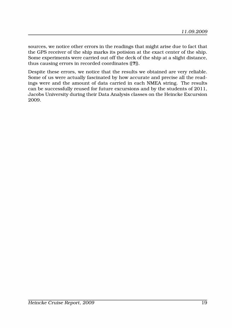
The ATLAS FANSWEEP 20/100 is a wide swath 100 kHz multi-beam echosounderdesigned for survey of coastal areas to depths of 600 m. It has a dual headtransducer that provides swath coverage of 6 times the water depth for bathymetryand up to 12 times the water depth for side scan imagery. It combines the ad-vantages of beamforming and interferometric phase measurement techniquesto the benefit of a large coverage together with high accurate depth measure-ments.
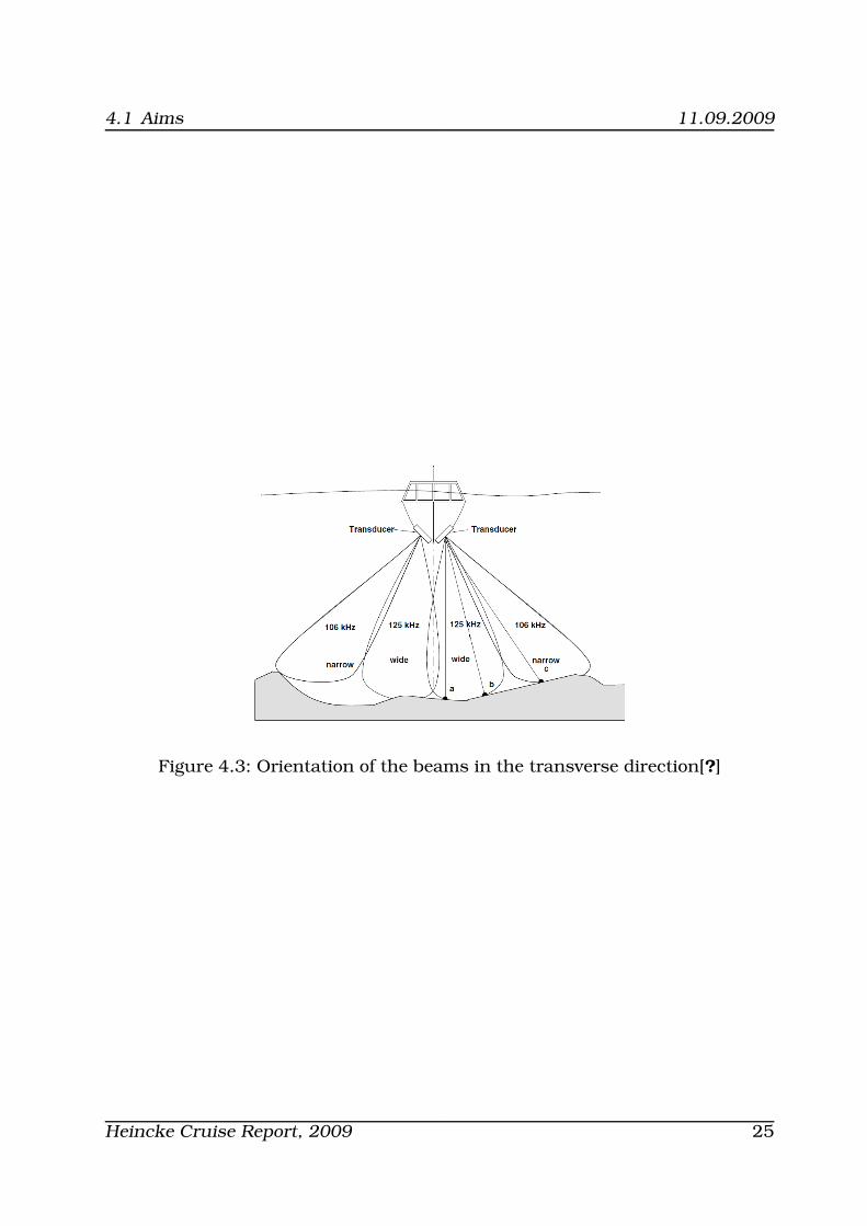
TRANSDUCER CONFIGURATION A pair of identical hydroacoustic transduc-ers is installed in the hull of the ship in V-shape. Each transducer consistsof 26 rows of elements arranged in two transmission sections and 10 recep-tion sections. Each section provides an inner beam (wide beam) and an outerbeam (narrow beam). Generally, all four beams are active but under extremelynoisy conditions (air bubbles or mud in the water column) the outer beamsare switched off in order to reduce the amount of erroneous echoes with highamplitudes.
Due to the specific form and arrangement of the beams, sound is directed fromeither side of the ship into the entire half-space from almost the horizontal tothe vertical. In all 4 beams, very short transmission pulses with the appropriatefrequency are transmitted at the same time. If, for example, it is assumed thatthe water bottom is flat and horizontal, the transmission pulses with the higherfrequency hit the bottom first (a). Parts of the bottom lying further away in thetransverse direction are reached later by the transmission pulse (b). The lower-frequency transmission pulses cover that part of the bottom that lies furtheraway in the transverse direction (c).
22 Heincke Cruise Report, 2009
4.1 Aims 11.09.2009
Figure 4.1: Setup of the instrument[?]
Heincke Cruise Report, 2009 23

11.09.2009 4 Multibeam
Figure 4.2: Flow diagram of the instrument[?]
24 Heincke Cruise Report, 2009
4.1 Aims 11.09.2009
Figure 4.3: Orientation of the beams in the transverse direction[?]
Heincke Cruise Report, 2009 25
11.09.2009 4 Multibeam
4.1.2 Measurement process
Each part of the water bottom that receives sound from the transmission pulsesends back an echo of greater or lesser strength. An echo of this kind arrives atthe reception staves at different times, depending on the direction of incidenceof the sound.
From the sound travelling time from the transducer to the bottom element andback, the slanting range between the bottom element and the transducer canbe calculated by means of the mean sound velocity, and finally the depth andthe lateral distance can be calculated from the slanting range and the anglerelative to the vertical. A necessary prerequisite here is that the sound velocityin the water at the location of the transducer must be known exactly, whichmeans that the temperature, salinity and pH have to be determined in advance.
26 Heincke Cruise Report, 2009

4.1 Aims 11.09.2009
Figure 4.4: Measurement process[?]
Heincke Cruise Report, 2009 27

11.09.2009 4 Multibeam
4.1.3 Accuracy of the instrument
• Measurement of Sound VelocityC-Probe determines the sound velocity directly by the measurement ofsound travelling time (the ”sing-around” method). If mud is depositedon the reflector of the sound travelling track, the track acts as if it hasbecome shorter and the sound velocity value determined can be too highby a considerable amount. Therefore, for data collection, the probe mustbe cleaned before use.
• Roll Angle Measurement with a Motion SensorThe longitudinal axis of the motion sensor should be arranged exactly per-pendicular to the transducer beams. Because the dynamic measurement-error of the motion sensor is less than 0.05 ◦, the angle error of the motionsensor should therefore be less than 0.3 ◦. If there is a trim error (angleerror), then when a ship is pitching, its pitch value acts to some extent asa roll error. If, on the other hand, the roll axis of the motion sensor is notexactly perpendicular to the transducer beams, which point in a directiontransverse to the sailing direction, the pitching motion has an effect in theroll axis of the motion sensor, and causes a roll measurement error.
Rollerror = arcsin[cos (E) ∗ sin (roll) − sin (E) ∗ sin(pitch)] − roll (4.1)
roll = true roll angle of the transducerE = angle error of the motion sensor roll axis compared to the true rollanglepitch = true pitch angle
• Measurement of the Course AngleIn the case of a multi-beam sweeping echosounder, the compass has thetask of presenting a bottom detail, e.g. an obstacle, at the correct positionin the coordinate system used. A compass installation error or a compasserror in general, affects the coordinate offset of an underwater object inthe sailing direction according to the following formula:
Coordinateoffset = distanceoftheobject ∗ sin (compasserror) (4.2)
The offset perpendicular to the sailing direction can be ignored.
28 Heincke Cruise Report, 2009

4.1 Aims 11.09.2009
4.1.4 Inclination of the Transducer’s Radiating Face Relative to the
Horizontal (100 kHz)
If the specified maximum depth is utilized: 50 ◦
In all other cases: 53 ◦
50 ◦ angles of installation have the effect that the area vertically under the shipalso produces strong echo levels. The coverage depends on the water bottom,and is often limited to just less than 6-fold, but in the case of mainly largemeasurement depths this leads to wide survey swaths for each track. In thecase of sea surveying, where the roll errors of the motion sensor reach the orderof magnitude of the FANSWEEP 20 measurement accuracy, larger coverageshave a reduced accuracy.
4.1.5 Effects of different installation positions of system
components
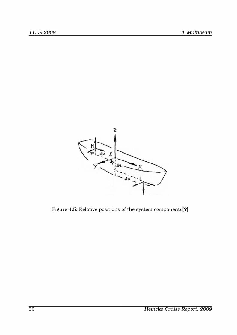
As the ship movement is related to the ship’s center of gravity, all resultingmovement, e.g. of the echosounder, need to be calculated. For this the posi-tions of the echosounder and the motion sensor in relation to the ship’s centerof gravity needs to be known. More than this the axes of sensors should bealigned to the ship’s co-ordinate system. The further away the motion sensoris installed from the echosounder, the more precisely the offset values have tobe determined, because the size of the error has a linear, distance dependanteffect.
The GPS unit is installed at a height of 17 m at the top of the research vessel.Motion Reference Unit is kept in the dry lab. Transducers are installed in thehull of the ship.
Heincke Cruise Report, 2009 29
11.09.2009 4 Multibeam
Figure 4.5: Relative positions of the system components[?]
30 Heincke Cruise Report, 2009

4.1 Aims 11.09.2009
4.1.6 Ship Movements
• HeaveHeave is a vertical translation along the z-axis. A varying coverage isalways the result of heave. Uncompensated heave produces a constantdepth error for the swath in the amount of the heave value.
• PitchPitch is the result of a rotation of the ship around the transverse axis(y-axis). Uncompensated pitch produces an error in depth and position.
Heincke Cruise Report, 2009 31

11.09.2009 4 Multibeam
Figure 4.6: Heave[?]
Figure 4.7: Pitch[?]
32 Heincke Cruise Report, 2009

4.1 Aims 11.09.2009
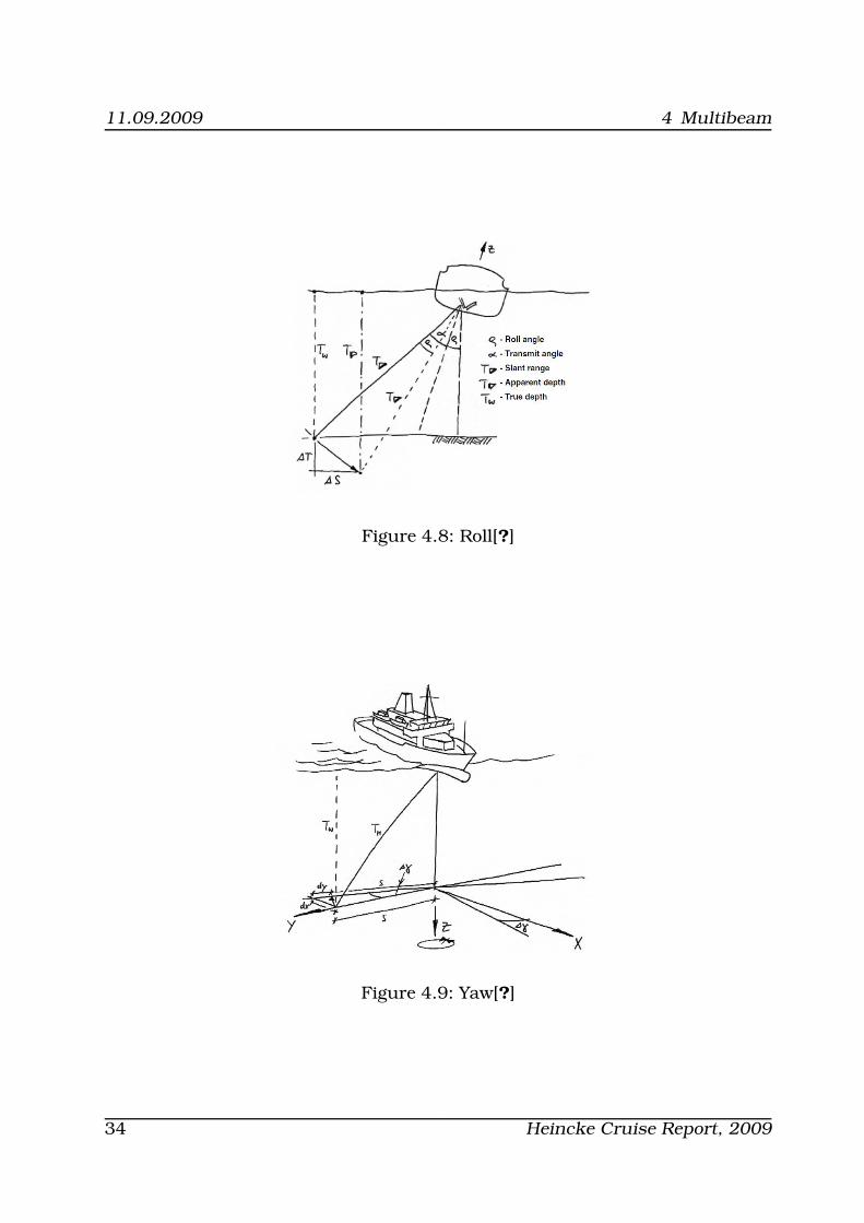
• RollRoll is the result of a rotation of the ship along the longitudinal axis (x-axis). Uncompensated roll produces an error in depth and position.
• YawYaw is rotation of the ship around the vertical axis (z-axis). Uncompen-sated yaw produces an error of the depth position.
Heincke Cruise Report, 2009 33
11.09.2009 4 Multibeam
Figure 4.8: Roll[?]
Figure 4.9: Yaw[?]
34 Heincke Cruise Report, 2009

4.1 Aims 11.09.2009
4.1.7 Coverage
The coverage is reduced, when the reflectivity decreases and the absorptionincreases. The pingrate decreases with increase in depths and coverages, be-cause the traveltimes of sound on the outer beams increases.
4.1.8 Sound Velocity
A wrong sound velocity produces depth error and dislocation of the positions. Ifthe setup value is less than the true sound velocity, then the depth calculated istoo small and if it is greater than the true sound velocity, the depth calculatedis too big.
4.1.9 Multibeam echosounder v/s Side scan sonar
Side scan sonar concentrates on the shadows being cast by its beam behindthe objects on the sea floor, while Multibeam Echosounder (MBES) focuses onthe resultant bathymetry for object detection. The low grazing angle of the sidescan sonar beam over the sea floor makes it good for object detection. ThoughMBES gives us high-resolution bathymetry, still post processing of the data isrequired to visualize results. The advantages of MBES over side scan sonar arethat the multibeam data is precisely georeferenced and the survey speeds arehigh.[?]
4.1.10 Method of data collection
As discussed in more depth in the next section, several variables affect thequality of the multibeam data including tides, salinity and pressure. Therefore,information for these variables needs to be collected so that it can be correctedfor in post-processing.
Also, information on tides are needed to correctly interpret the aquired data.As the data was taken near the German island Helgoland, the tides recordedon Helgoland are taken as a reference to correct for the tidal offsets in height.The values for salinity and pressure were acquired by a CTD conducted on thecruise.
The Motion reference unit used on this cruise was the TSS DMS 2i. It correctsfor roll, pitch, heave, and yaw which were explained in section ??. It startedworking effectively at 10:05 UTC time on Day 1.
Heincke Cruise Report, 2009 35

11.0
9.2
009
4M
ultib
eam
Profile Start End AverageNo. Date Time[UTC] Lon Lat[degrees] Date Time[UTC] Lon Lat[degrees] Speed[knots] Filename
1a 4.13.09 08:14:19 8.5779 53.5301 4.13.09 11:09:25 8.0923 53.8302 7.77 Helg1 00F1090413...sda
2b 4.13.09 11:09:43 8.0912 53.8435 4.13.09 12:50:03 7.7577 53.9974 9.78 Helg2 00F1090413...sda
3c 4.13.09 12:50:17 7.7577 53.9979 4.13.09 13:12:45 7.7571 54.0481 8.12 Helg3 00F1090413...sda
4 4.13.09 13:17:43 7.7590 54.0478 4.13.09 13:40:54 7.7578 53.9974 7.71 Helg4 00F1090413...sda
5 4.13.09 13:59:36 7.7563 53.9986 4.13.09 14:50:54 7.7804 54.0414 3.66 Helg5 00F1090413...sda
6 4.13.09 15:04:51 7.7825 54.0423 4.13.09 16:34:49 8.0646 54.0683 6.75 Helg6 00F1090413...sda
7 4.13.09 17:11:42 8.0844 54.0704 4.13.09 18:55:40 7.8943 54.1739 8.17 Helg3 00F1090413...sda
8 4.14.09 06:11:23 7.8985 54.1716 4.14.09 06:27:00 7.8938 54.1412 7.07 Helg8 00F1090414...sda
9 4.14.09 06:27:14 7.8936 54.1412 4.14.09 06:31:01 7.8938 54.1429 4.86 Helg9 00F10904140627.sda
10 4.14.09 06:33:06 7.8811 54.1442 4.14.09 06:49:13 7.8447 54.1528 5.12 Helg10 00F1090414...sda
11 4.14.09 06:49:26 7.8443 54.1530 4.14.09 07:18:20 7.8367 54.1540 1.13 Helg11 00F1090414...sda
12 4.14.09 07:33:44 7.8494 54.1519 4.14.09 07:39:09 7.8351 54.1505 2.88 Helg11 00F10904140733.sda
13 4.14.09 07:39:16 7.8349 54.1505 4.14.09 08:16:44 7.7392 54.1506 5.42 Helg13 00F1090414...sda
14 4.14.09 08:22:40 7.7387 54.1502 4.14.09 08:34:28 7.7390 54.1322 5.37 Helg14 00F1090414...sda
15d 4.14.09 08:34:34 7.7390 54.1321 4.14.09 09:46:11 7.7394 54.1323 4.56 Helg15 00F1090414...sda
16 4.14.09 09:46:21 7.7397 54.1323 4.14.09 09:56:20 7.7676 54.1319 5.95 Helg16 00F1090414...sda
17 4.14.09 11:15:54 7.9642 54.1318 4.14.09 12:52:49 7.9613 54.2450 5.34 Helg17 00F1090414...sda
18e 4.14.09 12:53:06 7.9612 54.2454 4.14.09 12:59:33 7.9632 54.2449 4.65 Helg18 00F10904141253.sda
19 4.14.09 12:59:44 7.9628 54.2448 4.14.09 13:34:50 7.8952 54.2453 5.15 Helg19 00F1090414...sda
20 4.14.09 13:35:49 7.8765 54.2467 4.14.09 13:37:06 7.8772 54.2487 5.78 Helg20 00F1090414...sda
21 4.14.09 13:54:55 7.8778 54.2633 4.14.09 13:56:47 7.8780 54.2661 5.45 Helg21 00F10904141354.sda
22 4.14.09 13:59:31 7.8801 54.2652 4.14.09 14:08:47 7.8797 54.2615 6.03 Helg21 00F10904141358.sda
23 4.14.09 14:11:38 7.8820 54.2505 4.14.09 14:20:41 7.8820 54.2653 5.93 Helg23 00F10904141411.sda
24 4.14.09 14:23:37 7.8841 54.2654 4.14.09 14:32:54 7.8838 54.2507 5.77 Helg24 00F10904141423.sda
25 4.14.09 14:35:40 7.8865 54.2506 4.14.09 14:40:09 7.8848 54.2579 5.91 Helg25 00F10904141435.sda
26 4.14.09 14:40:31 7.8847 54.2585 4.14.09 15:03:35 7.8204 54.2480 6.40 Helg26 00F1090414...sda
27 4.14.09 15:04:19 7.8182 54.2477 4.14.09 15:10:51 7.8007 54.2450 5.87 Helg27 00F10904141504.sda
28 4.14.09 15:11:22 7.7998 54.2449 4.14.09 16:05:54 7.8980 54.1714 7.21 Helg28 00F1090414...sda
aThere is a data gap from 09:04:01 to 10:05:56 due to resetting of the GYRO to correct the heading.bThere is a data gap from 12:24:37 to 12:46:29 as a result of the SURF data storage capacity being exceeded.cProfiles 3 and 4 were the calibration run.dNot a line but a big loop.eNot a line but a loop.
36
Hein
cke
Cru
ise
Report,
2009

4.2 Data Processing techniques 11.09.2009
4.2 Data Processing techniques
To view the data recorded with the multibeam as an image, the data has to beprocessed. Processing is subdivided into pre- and post processing steps.
The first step of processing is pre-processing. Pre-processing transforms theraw data into .sda files. This is done on the computer devoted to the multi-beam system and then the preprocessed data is transferred to challenger. Onecreated .sda file comprises data collected by the multibeam over a period of 10minutes. .sda files belong to the class of SURF files. SURF data files are 3Dscanner files. The reason why SURF files are convenient to use in this case isthe fact that they are open source and can be read by the program MBsystems,which is used for post processing and visualizing the data.
After the pre-processing, the data can already be visualized. Nevertheless itstill has to be corrected for measurement error sources, which is called postprocessing. Post processing and visualization is done using software calledMBsystems. MBsystems is an open source software package, which was de-veloped for the processing and display of bathymetry and backscatter imagerydata derived from multibeam, interferometry, and sidescan sonars.
The first thing the data should be corrected for is tides. As measurements aretaken over a period of time, sea level height will vary due to the tides. Thishas to be corrected for to find the true depth at every point of measurement.Ideally, one has a tide timetable for every spot on the track, which one cansubtract from the measurements taken. As this is not possible, because nosuch data is available, the data of the nearest location for which the tides areknown is used. As the data during this cruise was taken around Helgoland,the tidal heights measured on Helgoland were used for correcting for tides. Theprogram xtides was chosen to correct for tidal variations.
Another correction has to be made for the varying salinity and pressure con-ditions in the water column as they influence the velocity profile of the signal.Salinity and pressure conditions are usually unknown throughout the track.In this case, the salinity and pressure profile measured by a CTD during thecruise are taken and considered to be representative for all the area investi-gated.
Heincke Cruise Report, 2009 37

11.09.2009 4 Multibeam
Figure 4.10: Example of the recorded tides which are used by the programxtides to correct for tidal offsets.
38 Heincke Cruise Report, 2009

4.2 Data Processing techniques 11.09.2009
Figure 4.11: Calibration run going northward
Heincke Cruise Report, 2009 39

11.09.2009 4 Multibeam
Figure 4.12: Calibration run going southward
40 Heincke Cruise Report, 2009

4.2 Data Processing techniques 11.09.2009
As it is impossible to install the two transducers at a 50 angle by hand, onehas to account for little offsets in the setup as well. This is done by calibratingthe system. A calibration run is done by passing over a calibration area twice,but from different directions. The two images produced by the calibration runshould give exactly the same result for the seafloor topography. As it can beseen in Figure ?? and Figure ??, this is not the case for these measurements,meaning that the transducers are not at a perfect angle. This can be correctedfor by overlaying the results for the calibration run using the command MBcopyto figure out the offset-angle of the transducers. This angle correction can thenbe applied to all the data collected using the command MBedit.
In addition, the data has to be corrected for line drop outs, navigational errorsand in this case the GYRO, which was not working in the beginning.
Heincke Cruise Report, 2009 41

11.09.2009 4 Multibeam
4.2.1 Results and analysis
By looking at first images, one notices that not only large scale features, butalso small scale features such as shipwrecks are resolved very well on themultibeam image. In general, it appears that the seafloor is inclined, becausethe data has not been corrected for the angular offset of the two transducersyet.
42 Heincke Cruise Report, 2009

4.2 Data Processing techniques 11.09.2009
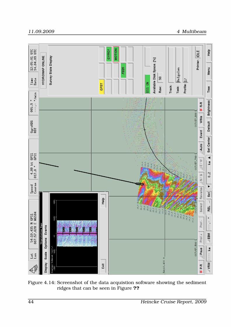
Figure 4.13: Sediment ridges in the north-west
Heincke Cruise Report, 2009 43
11.09.2009 4 Multibeam
Figure 4.14: Screenshot of the data acquistion software showing the sedimentridges that can be seen in Figure ??
44 Heincke Cruise Report, 2009

4.2 Data Processing techniques 11.09.2009
Figure 4.15: Shipwreck in the south-west at 54◦09′50”N7◦57′45”E
Heincke Cruise Report, 2009 45

11.09.2009 4 Multibeam
Figure 4.16: Screenshot of the data acquistion software showing the shipwreckthat can be seen in Figure ??
46 Heincke Cruise Report, 2009
4.3 Discussion and Conclusions 11.09.2009
4.3 Discussion and Conclusions
The data acquired seems to be of good resolution as even shipwrecks and sed-iment ridges can be seen clearly. It still needs to be corrected for height dif-ferences caused by tides and the angular offset of the transducers. Otherwisethere seems to be no major error source as the multibeam system was set upcorrectly and all the instruments were delivering good results, except for thegyro in the beginning. This might be a little difficult to correct for. Never-theless, the gyro was broken before the main area of interest was reached, soquality losses in that part of the data acquisition do not have severe conse-quences for the data. Also, there are two major data gaps in the beginning; onedue to the resetting of the GPS to make the gyro work, the other one because allthe data space on the hard disk was full and it had to be transferred to anothercomputer. But those two gaps occurred before the main area of interest wasreached and did not affect the calibration run. The data has to be correctedfor tides, the angular offset of the transducers, line drop outs and navigationalerrors. After the processing has been completed, the data should be comparedto already existing data. By doing so, one can look for major differences be-tween the data set which would hint at a major error source which has notbeen accounted for.
All in all, one can conclude that the system worked well, except for some minordifficulties in the beginning. The data acquired is of good quality as it resolveseven small scale features very well. Nevertheless, some processing work stillhas to be done on the dataset before it can be used for further research.
Heincke Cruise Report, 2009 47
11.09.2009 5 Sidescan Sonar
5 Sidescan Sonar
by Marta Gomez Betanzos
5.1 Aims
5.1.1 Instrument used, general principals of Side Scan Sonar
What is Side Scan Sonar
The basics of the Side scan sonar are the same as those of a normal sonar(sound, navigation, ranging). In this case, the side scan sonar is used to pro-duce an image of the seafloor topography as well as objects on the seafloor,like boulders, shipwrecks, sunken objects, sediment ripples, fish and morewhile being towed from behind, at a fair distance from the propeller, or, prefer-ably, at the side of the vessel a few meters (minimum 1 meter) above the seafloor surface. It is important that the Side Scan does not get too close to theseafloor, or else there is a risk of the tow fish hitting the ground and breakingoff. None-the-less, the closer to the seafloor and the slower the vessel is movingthe stronger the signal received and therefore the resolution of the scans. Sidescan sonar is also referred to as side-looking sonar or side-imaging sonar. Itcan scan hundreds of meters of seafloor on both sides of the tow fish withinreal time while producing a near-photographic quality image of the seabed. Itis referred to as ”side” scan since it emits sound waves to the sea floor at anangle rather than straight down. (See figures 1 and 2, or a and b respectively)
Side Scan sonar has many uses other than research and science purposes,namely -commercial, military, leisure,detection of mines and fisheries, lost ar-chaeological treasures and ship or plane wrecks among others.
48 Heincke Cruise Report, 2009

5.1 Aims 11.09.2009
Getting started
First thing one needs to do is to make sure everything is connected properly,with the exception of the Side Scan which should not be plugged in until it isactually being deployed. The items to be connected should be such that thepower supply (for both the control box and the console), GPS cable, and SideScan (later) are connected to the Side Scan surface interface SeaHub (the onereceiving the raw data); the surface interface SeaHub is then connected to theconsole (toughbook) which then interprets the data transmited by the surfaceinterface SeaHub box. (See figure 3) After this has been done we secure the towfish with the security hatch and safety pins so that they are fixed in place. Thetow fish is now ready to be put into the water and start recording. It might benecessary to install SeaNet Pro into the toughbook to be able to receive, recordand intrepret the data.
Heincke Cruise Report, 2009 49
11.09.2009 5 Sidescan Sonar
How does it work?
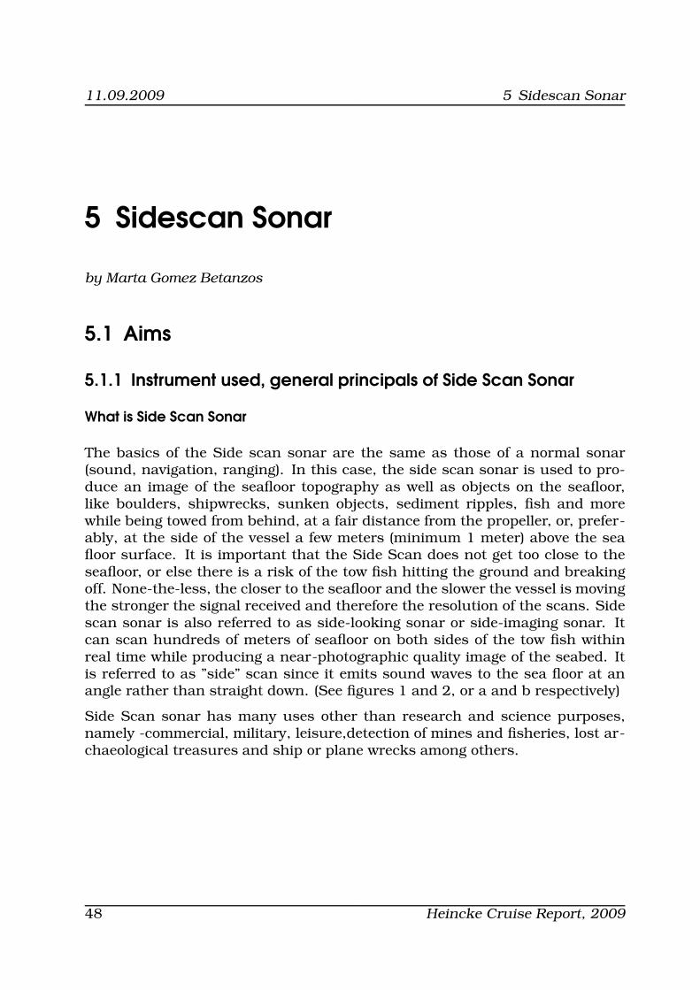
Side Scan Sonar consists of a sensor head(s), a control and a display soft-ware. The head transmits both high and low frequency so that high frequencieswill map the seafloor surface and specific structures and low frequencies sub-bottom imagery (depending on the type of sonar used, it is not always a given).As said above, Side scan sonar sends out a fan-shaped acoustic pulse whichis perpendicular to the direction of movement. The signal travels through thewater until it hits the seafloor or a solid structure(outcrop). The signal is thenbounced off and recorded by the tow fish along with the travel time, amplitudeand strength. These values are then sent to the console for further interpre-tation. In general terms, the console will use the values to produce a longcontinuous image of the mapped seabed (stored as .v4log files) as well as a realtime grey-scale image of the seafloor. The stronger signals will be shown aswhite areas, while the weakest, or zero, signals as shown as black; the restare scaled accordingly. (See figure 2) Strength of signal is defined by the slopeand the structure or material of the seafloor; so that stronger signals will be re-ceived when the seafloor slopes towards the tow fish and is made of bare rock.In contrast, weak signals will happen when the seafloor is covered with mud orsand and slopes away from the tow fish emitters. Furthermore, the image willalso show the shadows of the structures similarly to that of a flashlight shin-ing on the structure. (See figure 2) This is usually referred to as the acoustic
shadow of the object being mapped. (See Figure 4)
50 Heincke Cruise Report, 2009

5.1 Aims 11.09.2009
Working with the console. The toughbook
The most basic buttons when working with the toughbook are those that dealwith the image resolution of the raw data received from the Sonar. (See figure5). Starting from the left we have the setup menu which is self-explanatory,but will also be explained in more detail below. The on/off/pause button whichstarts, stops or pauses the data recording and image production (interpretationof data by the console); then the channel gain for both the left and right sideof the Sonar which set the Sonar receive gain and display contrast, so howsensitive the sonar receptor are to the receiving signal and the scale (in dB)or level of saturation. Sonar channel gain is usually set to 40% although itdepends entirely on the water conditions and on the type of sediment of theseafloor. Sonar display contrast also vary depending on the water conditions,though mostly on the speed of the vessel; such that one must pay attentionthat the dB indicators on either side are always larger than the red (left) andyellow (right) markers to avoid oversaturation of white. Next are the range,which defines the area of seafloor the Sonar beam covers/scans, the resolutionand the Frequency display. The resolution varies from low (Lo) to high (Hi) evenultra (Ult) if one wants a very detailed scan image of the seafloor, otherwise Med(medium) or Hi are the typical settings. As for the Frequency, the typical valueis 325Hz, and it defines the strength of the outward signal.
Heincke Cruise Report, 2009 51

11.09.2009 5 Sidescan Sonar
Some main features of the setup buttom mentioned above are the Cursor, Po-sition and Setup options. The cursor option tab brings out a box showing therange, data and time of a specific point on the Side Scan waterfall image. Theposition option tab sets the layback distance in meters between the tow fishand the vessel. Finally the setup option tab allows you to define several pa-rameters like the intensity sampling of Sonar data, painting the leading edgeof strong targets to emphasize sub-bottom layers, the units of display or thenumber of range ’bins’ sampled to the screen resolution. The range ’bins’ arethe sampled intervals; so every how many pulses the data is recorded, or inother words how often the recieved signals are sampled.
Interpreting Side Scan data iamges
So we know that only echoes of objects that reflect sound are recorded by theSide Scan sonar transducer. Burnished or smoothe surfaces and finer sedi-ments may not show too well on the echo image in a way that they may wipeout data from smaller structures nearby. In this way, clay and silts will bejust barely visible (low backscatter) as opposed to metals, boulders, gravel orrecently extruded volcanic rock which will give a high backscatter. Further-more, if the side scan is being towed too fast the signals will not be receivedas nicely as when towed at slower speeds. Other than that, data from texture,structure and size of the objects is very nicely recorded and reproduced by theconsole. Knowing the strength of the receiving signal, one can examine thecomposition of the seafloor and any other structures or object. A sketch of atypical Side Scan sonar scanline would be as shown in figures 6 and 7,or a andb respectively.
Interpreting Side Scan sonar data is something that comes with experience andpractice, and while reflections of small objects are harder to interpret, man-made structures like platforms or rock walls are easier to interpret due to theirregular patterns.
The bottom line of using and interpreting Side Scan Sonar data is that you haveto approach it as if looking at the world through a shiny black plastic with aflashlight’s torch beam as the only source of light. Regarding the maintenance,it is important to wash the instrument (cable and tow fish) with fresh waterafter each deployment, making sure that it is rinsed properly of all (or most of)the salt water. Furthermore, the instrument, namely the tow fish, should notbe exposed to extreme conditions.
52 Heincke Cruise Report, 2009

5.1 Aims 11.09.2009
Advantages and Limitations to Side Scan Sonar
Side Scan Sonar is a very useful tool for mapping the seafloor, especially inturbid waters, since structures, sediment types such as mud, sand, ripples,outcrops, boulders, canyons, buried objects, and even fish can be detected.Dense objects like rocks, coarse sand and metal will be reflected best by givingoff a stronger signal; soft features like mud, sand, silt produce weaker signalssince they actually absorb the sonar energy. However, regardless of it quali-ties Side Scan Sonar also has some limitations, -namely those related to thedepth, strength of signal, data collection and interpretation, and resolution ofthe image produced based on the conditions of speed and distance to seafloor.
Heincke Cruise Report, 2009 53

11.09.2009 5 Sidescan Sonar
5.1.2 Method of data collection (list of line and line numbers
collected)
54 Heincke Cruise Report, 2009

5.1 Aims 11.09.2009
Figure 5.1: Table with the results obtained for April 14th showing start date,time and Latitude (Lat.) and Longitude (Long.) End date, time andLatitude (lat.) and Longitude, and file(s) corresponding to each line.Each line was done with the tow fish at 28 marks distance (withtwo marks having a distance of 1 meter)from the side of the vessel.Start time and end time were taking from the Console UTM; realtime is 2 hours more of that shown on the table.
Heincke Cruise Report, 2009 55

11.09.2009 5 Sidescan Sonar
5.2 Data Processing Techniques
In our case the data was collected by using a Tritech SeaKing Towfish SideScan Sonar System (toughbook console, interface surface SeaHub box, SideScan and corresponding cables (side scan, power supply, GPS)). For the mostpart the general conditions were:
- Left gain and display contrast: 44-53% (namely 44%, 50% and 53%) and47dB
- Right gain and display contrast: 41 - 67% (namely 41%, 47%, 63%) and47dB
- Range 100 m or 200 m
- Resolution: Ult
- Frequency: 325 Hz
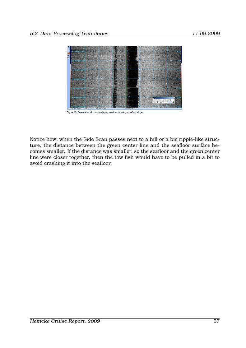
The parameters, -namely the left and right channel gain and display contrast-, had to be changed according to the vessel’s speed, so that there were notany areas of white oversaturation or to avoid horizontal lines cutting acrossthe data and giving ”bad” data. Furthermore, the tow fish had to be pulledup sometimes to avoid it getting too close to the seafloor. During the stops forCTD, sediment samples, or when the small boat was launched and the vesselwas stopped, the Tow fish had to be pulled in beforehand so that it did not getcaught in the propeller or hit the seafloor. All data were collected on the 14thApril, with the exception of the practice line (line No. 0) which was done on April13th. Lines were named by the captain of the vessel according to the trajectorydefined by the Navigation group. Due to the extremely large size of the datafiles, the lines had to be stopped and restarted every so often to avoid havinghuge unreadable files. The data was saved as .4vlog files and then convertedto .XTF, .TIF (.GEOTIFF), and if possible to .KML (for Google Earth viewing).Looking at the display window data on the seafloor, sediments and outcropstructures where recorded to the sides leaving a blind band of data which wasthe area directly underneath the Side Scan. This area is really important tohave under more or less constant surveillance, since it will tell you how closethe tow fish is to the seafloor, and therefore warn you in case you have to pullit in a bit. Basically, what happens is that if the middle of the Side Scan path(a.k.a the vessel’s trajectory line) and the first line of receiving signals comeclose together then the tow fish is practically on the seafloor and needs to bepulled in urgently. Take for example the following screenshot (see figure 13):
56 Heincke Cruise Report, 2009
5.2 Data Processing Techniques 11.09.2009
Notice how, when the Side Scan passes next to a hill or a big ripple-like struc-ture, the distance between the green center line and the seafloor surface be-comes smaller. If the distance was smaller, so the seafloor and the green centerline were closer together, then the tow fish would have to be pulled in a bit toavoid crashing it into the seafloor.
Heincke Cruise Report, 2009 57
11.09.2009 5 Sidescan Sonar
5.2.1 Results and Analysis
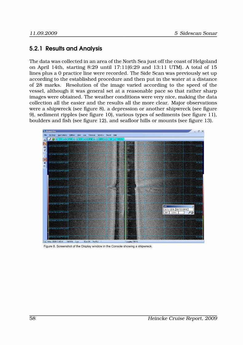
The data was collected in an area of the North Sea just off the coast of Helgolandon April 14th, starting 8:29 until 17:11(6:29 and 13:11 UTM). A total of 15lines plus a 0 practice line were recorded. The Side Scan was previously set upaccording to the established procedure and then put in the water at a distanceof 28 marks. Resolution of the image varied according to the speed of thevessel, although it was general set at a reasonable pace so that rather sharpimages were obtained. The weather conditions were very nice, making the datacollection all the easier and the results all the more clear. Major observationswere a shipwreck (see figure 8), a depression or another shipwreck (see figure9), sediment ripples (see figure 10), various types of sediments (see figure 11),boulders and fish (see figure 12), and seafloor hills or mounts (see figure 13).
58 Heincke Cruise Report, 2009

5.2 Data Processing Techniques 11.09.2009
Figures 8 and 9 show what is definitely a shipwreck in figure 8 and what mightbe a shipwreck, a sunken object or a depression in figure 9. Observe howin figure 8 the bow and stern of the sunken ship are clearly distinguishable.Furthermore, the trace of the trajectory it followed at the time of sinking is alsoobserved in the surrounding dent on the seafloor sediments. The middle partof the ship is within the Sonar’s ”blind spot”, so that no data, and thereforeimage, was obtained.The same more or less applies for the structure in figure 9, although in thiscase it is less obvious what it is. The problem here was that the console frozeand this was the only data that was recorded. None-the-less, we can see theacoustic shadow of what looks to be obviously some sunken object, whether itbe a ship or something else, or a depression in the seafloor surface.
Heincke Cruise Report, 2009 59

11.09.2009 5 Sidescan Sonar
Figure 10 shows very nice sediment ripples on both sides of the Side ScanSonar. Notice the lighter areas corresponding to the stronger signals bouncingoff the top of the ripples and off the slope facing the Side Scan. The darkerbands correspond to the backside of the sediment ripple where the frequencysignals either do not reach or simply bounce off in directions opposite to theSonar’s receptors. It is also shown that there is a slight elevation of the seafloorsince the Side Scan blind spot is temporarily narrowed down.
60 Heincke Cruise Report, 2009

5.2 Data Processing Techniques 11.09.2009
In figure 11, very clear sediment types are visible. Considering that lighterareas correspond to stronger signal reception and that strong signals are typ-ical of harder sediments, like rocks, coarse sand, metals, boulders, gravel orrecently extruded volcanic rock; then we can assume that it has to be one ofthose; although it is most likely coarse sand, rocks and boulders (which weactually saw (see figure 12)) or gravel for the lighter colored patches and mudor silt for the darker patches.
Heincke Cruise Report, 2009 61
11.09.2009 5 Sidescan Sonar
As mentioned above, one of the sediment structures of the area has to becomposed of boulders, since otherwise a weaker signal would be received andshown accordingly on the image.Proof that boulders are part of the sedimentsin the area covered is shown in figure 12, where we see lighter spots with thecorresponding acoustic shadows which correspond to boulders on the seafloor.These lighter areas show higher surfaces which stand out from the seafloorsurface as outcrops. Furthermore, the acoustic shadow only serves to giveeven more proof that there is an outcrop or some sort of structure standing outfrom the surrounding smooth seafloor surface. Also in figure 12, we can seesome fish swimming within the Side Scan’s ”blind spot”. Still using some ofthe old technology present in the traditional depth sounders, side scan sonarscan still receive signals coming from directly below the tow fish. Fish, as anyother object will reflect and send signal back to the sonar’s receptors. The factthat there is a so-called ”blind spot” right under the sonar means only that thesignal received will not be as accurate as those bouncing back from object lo-cated to the sides of the sonar’s path. Initially the Side scan sonar was also sedto receive signals from directly below it, but with the development of the sonartechnology the traditional single-beam depth-sounder was replaced by the sidescan sonar, which ”speciallized” in listening to the echoes recieved from eitherside of the tow fish and not so much on what is directly beneith it. In time, thedevelopment of the multi-beam made this distinction less meaningful. Regard-less of, side scan sonars also pick up on what is present in the water column,so any small grey-ish areas are all the small particles and organisms(such asfish or plankton) found in the water column.
Finally, figure 13 shows some clear seafloor hills that tend towards the SideScan’s trajectory, implying that we are probably cruising right on top of them;which is also why only half of the hill is visible. Here too the slope that tendstowards the direction of the Side Scan (so facing it) is shown as lighter coloredwhereas the acoustic shadow where no data is received is shown as dark areas.One could also argue that, due to the obvious symmetry between the four largerpeaks, the so-called hills could be either an agglomeration of sea mounds ortwo rows of individual sea mounds running almost parallel to each other. Butthat sounds like too much coincidence. It could also be that the tow fish wentover what would be a ridge, or sediment waves. Looking at the image (figure13) one can distinguish some darker areas which are slightly more elevated andwhich lead to the so-called hills. Due to the symmetry in the bumps it seemsmore probable that they are parts of a ridge.Also in the screenshot are traces or marks of different sediment types.
Some examples of survey lines that were able to be converted to .TIF (or .GEO-TIFF) via the program Seanet Dumplog are:
62 Heincke Cruise Report, 2009

5.2 Data Processing Techniques 11.09.2009
Figure 2 shows what a typical survey line looks like. No major features areobserved, but it is still a very nice survey line to have as an example. Somehills and ups and downs of the seafloor are visible.
On the left-hand side of this survey line (figure 3) we can see the seafloor hills,mounds or larger ripples explained before for the screenshot for figure 13.Black lines tend to represent missing or bad data. However, the appearance
Heincke Cruise Report, 2009 63

11.09.2009 5 Sidescan Sonar
Figure 5.2: Side Scan Sonar survey line data file (.v4log) as an image file (.GEO-TIFF).
Figure 5.3: Side Scan GEOTIFF image showing some seafloor hill-like struc-tures to the left-hand end of the image.
of major sections of bad data were rare and only on counted occasions.
Survey line Tue 14 Apr 12 59.TIF (file surveyline 10 43.eps) apperas to be toolarge to be worked with in latex; none-the-less it has been uploaded with therest of the data files in the challenger folder. The .GEOTIFF image shows whatin figure 11 were described as different sediment types along the line goingfrom 429068.327E, 5998787.195N to 4322395.91E, 5998798.946N. They ap-pear as lighter colored areas (light green-yellowish areas) showing that thereis a change of the receiving signal strength, which in turn implies a change inseafloor composition.
64 Heincke Cruise Report, 2009

5.3 Discussion of some of the features observed 11.09.2009
5.3 Discussion of some of the features observed
Some of the most interesting features observed in the course of the day were thevery obvious shipwreck, the sunken object which was said to be another ship-wreck although less obvious, the sediment ripples and types, and the seafloorhills. Some boulders and fish were also observed, but not too clearly. Regardingthe first shipwreck (see figure 8) one could see a clear image of the bow, sternand dent on the seafloor of the ship. Judging from the dent on the sediment wecan theorize how the ship sunk, or on the bottom water current; the directionin which the ship is given by where the bow if pointng as well as by the changein depth of the dent on the seafloor. Furthermore the same grey-scale imageon the Side Scan console was obtained with the multibeam, although in thiscase the different heights showed up as different color layer instead of the greyscale that accompanies the signal strength of the Side Scan Sonar. The samewas observed for the second so-said shipwreck, although one would be moreinclined to say that is it simply some sunken object which due to punctualmalfunctioning of the console was just barely observed (see figure 9). In thiscase the deeper areas surrounding the object are clearly visible; matter-of-fact,since there is a darker area enclosed between two lighter areas one would betempted to say that it is rather some sort of depression in the seafloor, be it bythe impact of some heavy object or due to biological or geological process; al-thugh once more this is only another hypothesis for the observed data. As withthe previous case, the multibeam also registered it as a colored image showingheights via a color scale instead of in a grey scale. Still on the seafloor surface,we also saw some hills or mounds on the inner rim of the Side Scan Sonaracoustic signal fan. This implies that, as said above, the Side Scan cruisedright on top of them, thus only capturing half of the hilly structures. We knowthat they are hills or mounds since surface height increases, making the SideScan acoustic fan temporarily larger due to proximity to the seafloor. Also ifone looks at the data (see figure 13) it is obvious that there is some sort ofoutcrop rising above the seafloor surface. Another hypothesis is that the ob-served hilly structures are really the ends of a small like ridge on the seafloor,some sort of larger sediment ripple-like structure. This is also possible, sinceif we take a close look at the figure, we see that the same structures show onboth sides of the Side Scan at more or less same latitude, as if parallel to eachother; suggesting the start and end points of a ripple-like structure like thoseobserved in figure 10, although these are smaller more abundant ripples mostprobably formed by seafloor waves due to movement of water masses near theseafloor.
Moving into the sediment,just slightly below the seafloor surface, we see thatthe Side Scan actually picked up on different types of sediment compositions.This is very clear in figure 11, where different grey-scales define the strength of
Heincke Cruise Report, 2009 65
11.09.2009 5 Sidescan Sonar
the signal and therefore the hardness or softness of the sediment scanned. Inthe case of figure 11, we see lighter patches which most probably correspondto harder more reflective sediments such as gravel, rock, or coarse sand. Onthe lower part of the image and in between some of the lighter patches, we seedarker areas which correspond to soft sediments; such that the signals wereabsorbed by the sediment instead of completely reflected. This then suggestsome type of clay/mud, silt or fine grained sand. It was said that some bouldersand fish were observed, but as explained above they were not very clear. Theboulders where seen as small lighter shaded areas with their correspondingacoustic shadow, and the fish were seen as isolated signal reception within theSide Scan path.
66 Heincke Cruise Report, 2009
5.4 Conclusion 11.09.2009
5.4 Conclusion
The Side Scan Sonar was created in the 1950’s for military purposed by Ger-man scientist, Dr. Julius Hagemann. It is also sometimes referred to as Side-looking Sonar or Side-imaging Sonar due to the fact that it only scans theareas to the side of the tow fish and not those directly below it. It has sev-eral frequency, range and resolution parameters as well as gain and displaycontrast values which can be modified according to the water conditions, thespeed of the vessel and the aim of the scan; such that fast scans will use lowerresolution, larger range areas, and possibly faster frequency signals to obtainthe best possible image from a quick and broader glance at the seafloor sur-face. The opposite will hold for more detailed scans of the seafloor surface.The general principal behind the side scan is that it sends out regular acoustic(frequency) signals which will bounce back, in a stronger or weaker manner,and be recorded by the Sonar receptors. The data, containing strength, timeelapsed and amplitude of the signal, will then be sent to the surface interfaceand interpreted by the console, which will produce a grey-scaled image of theseafloor surface as the Side Scan is towed along. The survey line is also savedand can then be converted to image files so that they can also be viewed onprograms such as Google Earth, in a way similar to how imaged from the GPSare plotted to produce a constantly update view of the world. The lab coursewas carried out from the 13th April to the 15th April off the coast of Helgoland,although data was only collected on April 14th. A trial run (line No. 0) was doneon April 13th as practice and system check up for the next day. This surveyline was actually run for a long time, which let me know that they should bestopped every so often and restarted to avoid huge data files. None-the-less,during that first run nothing much was observed, and it was not until the nextday that some more interesting findings such as a shipwreck, sediment ripples,hills/mounds/big ripples or ridges on the seafloor (from my perspective, andupon further inspection of the images, they are more like big ripples than in-dividual hills), different sediment types as well as some boulders and fish wereseen. A second sunken object was spotted, although the console temporarilyfroze and not too much was recorded for the area. It did however appear to besome sort of object, although I am more inclined to say that it looks more like adepression or a dent in the seafloor surface, since a clear lighter colored rim isvisible around a darker shaded middle area. Some Very nice sediment rippleswere also observed.
Limitations to the Side Scan are namely the speed of the vessel, the water con-ditions such as turbidity; sediment composition, since soft sediments will ab-sorb the signals and limit the amount of signals, and therefore data, recorded;and depth of the Side Scan with regard to the depth of the seafloor; the closerto the seafloor the better the image resolution and data collection, however the
Heincke Cruise Report, 2009 67
11.09.2009 5 Sidescan Sonar
risk of the tow fish hitting an outcrop or the seafloor itself is too big to make itworthwhile, since the instrument would be lost. But not only the tow fish, thewhole setup can give problems; as happened with us when the console frozeand had to be rebooted. Data can also be lost if the tow fish passes over acable or pipe that runs through the seafloor, in which case a horizontal line willcross the whole data and ruin the scan-lines in that latitude. None-the-lessthere are also many advantages to the Side Scan Sonar, namely- it’s impressiveaccuracy for mapping the seabed, seafloor structures and outcrops, sedimenttypes, and sunken objects. It is most useful when working in turbid waters,where visibility is very limited.
68 Heincke Cruise Report, 2009
5.5 References 11.09.2009
5.5 References
5.5.1 Text references
NOAA. Office of Coast Survey, ”Side Scan Sonar.” Learn About Hydrography.2009. United States Office of Coast Survey. 26 May 2009. http://www.nauticalcharts.noaa.NOAA. Coastal Services Center, ”Side Scan Sonar.” Benthic Habitat Mapping.2009. United States Office of Coast Survey. 26 May 2009. http://www.csc.noaa.gov/benthicStarfish. The seabed is your playground. ”WHAT IS SIDE SCAN SONAR?’.”Starfish. Seabed Imaging Systems. 2009. Tritech International Limited. 26May 2009. http://www.starfishsonar.com/technology/sidescan-sonar.html.Tritech International Ltd, ’Tritech SeaKing Towfish Side Scan Sonar System.”Tritech Side Scan Sonar Systems”. 2009. 26 May 2009. http://www.tritech.co.uk/produWoods Hole Oceanographic Institution, ”Side-Scan Sonar Images.” Voyage toPuna Ridge. 1998. Woods Hole Oceanographic Institution. 26 May 2009.http://www.punaridge.org/doc/factoids/Default.html.
5.5.2 Image references
Figures 1 and 2 were taken from Woods Hole Oceanography Institution Voyageto Puna Ridge.Figure 3 was made by me.Figure 4 was taken from Woods Hole Oceanography Institution Voyage to PunaRidge, although I did some editing on it.Figure 5 was taken from page 16 of issue 1 of the Tritech International LtdSeaKing Side Scan Sonar System manual.Figures 7-13 are screenshots taken from the Side Scan Console.Survey line images were taken from the Challenger folder where all the dataand files pertaining to the Heincke excursion are uploaded.
Heincke Cruise Report, 2009 69

11.09.2009 6 Marine Magnetics
6 Marine Magnetics
by Milen Iliev and Kin Ovanesov
6.1 Aim
The aim of this experiment was to use a ship-towed SeaSpy magnetometer tocreate a magnetic field profile of the area directly south of the island of Hel-goland, encompassing the waters between 7◦ and 8.2◦ E, along the 54th northparallel. Two separate lines were measured in the course of two days, eachroughly parallel to 54◦ N, during the time of the day, when the geomagneticfield was relatively stable. Data was gathered at a measurement rate of 1 Hz,and was processed by having observatory values of the geomagnetic field sub-tracted from it. A plot for each line was created, and major anomalies wereidentified and discussed.
6.2 Theory
Magnetic Field
Magnetic fields are produced by electric currents, which can be macroscopiccurrents in wires, or microscopic currents associated with electrons in atomicorbits. The magnetic field B is defined in terms of force on moving charge inthe Lorentz force law. The interaction of magnetic field with charge leads tomany practical applications. Magnetic field sources are essentially dipolar innature, having a north and south magnetic pole. The SI unit for magnetic fieldis the Tesla, which can be seen from the magnetic part of the Lorentz forcelaw Fmagnetic = qvB to be composed of N ·s
C·m. A smaller magnetic field unit is the
Gauss (1 Tesla = 10,000 Gauss).
Both the electric field and magnetic field can be defined from the Lorentz forcelaw:
F = qe︸︷︷︸
electrical force
+ qv ×B︸ ︷︷ ︸
magnetic force
(6.1)
70 Heincke Cruise Report, 2009

6.2 Theory 11.09.2009
Magnetic Field Strength (H) The magnetic fields generated by currents andcalculated from Ampere’s Law or the Biot-Savart Law are characterized bythe magnetic field B measured in Tesla. But when the generated fields passthrough magnetic materials which themselves contribute internal magneticfields, ambiguities can arise about what part of the field comes from the ex-ternal currents and what comes from the material itself. It has been commonpractice to define another magnetic field quantity, usually called the ”magneticfield strength” designated by H. It can be defined by the relationship
H =B0
µ0
=B
µ0
− M (6.2)
It unambiguously designates the driving magnetic influence from external cur-rents in a material, independent of the material’s magnetic response. The rela-tionship for B can be written in the equivalent form
B = µo(H + M)
H and M will have the same units, Am
. To further distinguish B from H, B
is sometimes called the magnetic flux density or the magnetic induction. Thequantity M in these relationships is called the magnetization of the material.[?]
Magnetic Properties of Solids
Materials may be classified by their response to externally applied magneticfields as diamagnetic, paramagnetic, or ferromagnetic. These magnetic re-sponses differ greatly in strength. Diamagnetism is a property of all materialsand opposes applied magnetic fields, but is very weak. Paramagnetism, whenpresent, is stronger than diamagnetism and produces magnetization in the di-rection of the applied field, and proportional to the applied field. Ferromagneticeffects are very large, producing magnetizations sometimes orders of magni-tude greater than the applied field and as such are much larger than eitherdiamagnetic or paramagnetic effects.
The magnetization of a material is expressed in terms of density of net mag-netic dipole moments µ in the material. We define a vector quantity called themagnetization M by
M =µtotal
V(6.3)
Another commonly used form for the relationship between B and H is
B = µ0H (6.4)
whereµ = µm = Kmµ0
Heincke Cruise Report, 2009 71

11.09.2009 6 Marine Magnetics
µ0 being the magnetic permeability of space and Km the relative permeability ofthe material. If the material does not respond to the external magnetic field byproducing any magnetization, then Km = 1. Another commonly used magneticquantity is the magnetic susceptibility which specifies how much the relativepermeability differs from one.
Magnetic susceptibility χm = Km − 1
For paramagnetic and diamagnetic materials the relative permeability is veryclose to 1 and the magnetic susceptibility very close to zero. For ferromagneticmaterials, these quantities may be very large.
The unit for the magnetic field strength H can be derived from its relationshipto the magnetic field B, B = µH. Since the unit of magnetic permeability µ isNA2 , and then the unit for the magnetic field strength is:
TN/A2
=N
AmNA2
=A
m
An older unit for magnetic field strength is the oersted: 1A/m = 0.01257oersted.[?]
6.2.1 The Earth’s Magnetic Field
When describing the magnetic field strength of the earth, it is more common touse units of nanoteslas (nT), where one nanotesla is 1 billionth of a tesla. Theaverage strength of the Earth’s magnetic field is about 50,000 nT.
Magnetic Equator - The location around the surface of the Earth where theEarth’s magnetic field has an inclination of zero (the magnetic field vector F ishorizontal). This location does not correspond to the Earth’s rotational equator.
Magnetic Poles - The locations on the surface of the Earth where the Earth’smagnetic field has an inclination of either plus or minus 90 degrees (the mag-netic field vector F is vertical). These locations do not correspond to the Earth’snorth and south poles.
As observed on the surface of the earth, the magnetic field can be broken intothree separate components.
Main Field
This is the largest component of the magnetic field and is believed to be causedby electrical currents in the Earth’s fluid outer core (dynamo). For exploration
72 Heincke Cruise Report, 2009
6.2 Theory 11.09.2009
work, this field acts as the inducing magnetic field. Circulation in core changeswith time: secular variations.
External Magnetic Field
This is a relatively small portion of the observed magnetic field that is gener-ated from magnetic sources external to the earth. This field is believed to beproduced by interactions of the Earth’s ionosphere with the solar wind. Hence,temporal variations associated with the external magnetic field are correlatedto solar activity. Changes with time: diurnal variations.
Crustal Field
This is the portion of the magnetic field associated with the magnetism ofcrustal rocks. This portion of the field contains both magnetism caused byinduction from the Earth’s main magnetic field and from remanent magnetiza-tion, which is the magnetic field element, that was ’locked’ in the rock when itlithified or crystalized..
The magnetic field varies with time.
Secular Variations - These are long-term (changes in the field that occur overyears) variations in the main magnetic field that are caused by fluid motion inthe Earth’s Outer Core. Because these variations occur slowly with respect tothe time of completion of a typical exploration magnetic survey, these variationswill not complicate data reduction efforts.
Diurnal Variations - These are variations in the magnetic field that occur overthe course of a day and are related to variations in the Earth’s external mag-netic field. This variation can be on the order of 20 to 30 nT per day and shouldbe accounted for when conducting exploration magnetic surveys.
Magnetic Storms - Occasionally, magnetic activity in the ionosphere will abruptlyincrease. The occurrence of such storms correlates with enhanced sunspot ac-tivity. The magnetic field observed during such times is highly irregular andunpredictable, having amplitudes as large as 1000 nT. Exploration magneticsurveys should not be conducted during magnetic storms.
Magnetics and Geology
The induced field relates to the existence of rocks of high or low magnetic sus-ceptibility near the instrument. If measurements are taken near rocks of highmagnetic susceptibility, magnetic field of higher strength will be measured. Thestrength of the field will decrease if the measurements will be taken at a greaterdistance from rocks of high magnetic susceptibility.
[?]
Heincke Cruise Report, 2009 73

11.09.2009 6 Marine Magnetics
6.3 Instruments: The Magnetometer
The magnetometer which was used (SeaSPY) is a Total Field magnetometers,i.e. it measures only the magnitude of the magnetic field vector, independent ofits direction with respect to the sensor. In comparison Vector magnetometershave the ability to measure the component of ambient field that is projectedalong one dimension in space. In order to calculate the total field, three sep-arate vector magnetometer sensors must be oriented at right angles to eachother, and their outputs geometrically added by a single processor. There aresome practical limitations to how precisely and how rigidly the three sensorscan be fixed together at exactly right angles. This is the reason, why the total-field precision of even the best flux-gate magnetometers is limited to an orderof magnitude less than a SeaSPY magnetometer. Also the output of all vector-field sensors will experience drift with the time and with temperature. Vectormagnetometers require periodic calibration with an accurate reference such asa proton-spin magnetometer. Proton-spin magnetometers never require cali-bration.These are the reasons, why total-field magnetometers are inherentlysuperior to vector magnetometers when the task is detection of ferromagneticanomalies within the Earth’s magnetosphere.
A standard proton-spin magnetometer sensor begins with a small volume ofproton-rich fluid such as methanol. Polarization of the protons in the fluid iscaused through induction of a large temporary artificial magnetic field aroundthe liquid. Once the proton population has been polarized, the proton spinaxes are stimulated to precess around the ambient magnetic field vector. Thisprocess is known as deflection. The alternating magnetic field generated byproton precession may be detected by a coil, and its frequency measured bythe magnetomeric electronics. This frequency is directly proportional to themagnitude of the ambient field vector.
The difference between proton and Overhauser magnetometers is most appar-ent in the way that the proton populations are biased. The Overhauser effect isa phenomenon that uses electron-proton coupling to achieve proton polariza-tion. SeaSPY Overhauser magnetometer sensors can produce clear and strongproton precession signals using only 1-2W of power. In contrast, standardproton sensors cannot produce signals that approach the same order of mag-nitude. SeaSPY’s resolution is 0.001nT and it is highly sensitive and accurate(0.1nT) in comparison to the proton magnetometers. [?]
74 Heincke Cruise Report, 2009

6.4 Data Collection 11.09.2009
6.4 Data Collection
Data was collected in two runs, on two consecutive days. The towfish was towedby its cable from a small boat at a distance of around 70 m. The boat itselffollowed the Heincke at a variable distance of 80 to 120m, so that magneticinterference from the ship’s hull is minimized. Figure ?? describes the physicalsetup of the equipment.
Figure 6.1: Physical setup of the magnetometer measurements.
The system for powering the magnetometer and recording the data was housedin a briefcase, which contained a DC battery power unit, an AC converter, aTouhgbook laptop, and a GPS receiver. The towfish, the laptop and the GPSreceiver all received their power from the converter. Data was passed from theGPS receiver and the towfish to the laptop. Figure ?? illustrates the setup ofthe system.
The properties of the lines are summarized in the tables below (Tables ?? and??):
Line 1:
Filename:Line 1.xls
Date Time (UTC) Latitude (◦N) Longitutde (◦E)
Start April 13, 2009 15:08:06 54.042347 7.782093
End April 13, 2009 16:52:04 54.073143 8.115106
Table 6.1: Table, summarizing relevant data for Line 1.
Line 2:
Filename:Line 2.xls
Date Time (UTC) Latitude (◦N) Longitutde (◦E)
Start April 14, 2009 09:47:20 54.13202 7.737297
End April 14, 2009 10:57:58 54.13267 7.957056
Table 6.2: Table, summarizing relevant data for Line 2.
Heincke Cruise Report, 2009 75
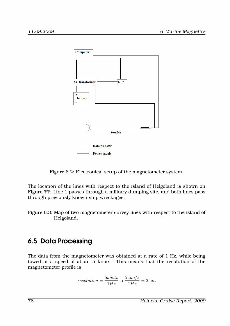
11.09.2009 6 Marine Magnetics
Figure 6.2: Electronical setup of the magnetometer system.
The location of the lines with respect to the island of Helgoland is shown onFigure ??. Line 1 passes through a military dumping site, and both lines passthrough previously known ship wreckages.
Figure 6.3: Map of two magnetometer survey lines with respect to the island ofHelgoland.
6.5 Data Processing
The data from the magnetometer was obtained at a rate of 1 Hz, while beingtowed at a speed of about 5 knots. This means that the resolution of themagnetometer profile is
resolution =5knots
1Hz≈
2.5m/s
1Hz= 2.5m
76 Heincke Cruise Report, 2009

6.5 Data Processing 11.09.2009
Data supplied by the magnetometer had a time stamp and a total magneticfield value. The system then obtained the proper longitude and latitude foreach measurement from the GPS receiver system. Thus, the files have theformat of a Spreadsheet with columns for date and time, longitude, latitude,and total magnetic field strength.
It should be noted, however, that by this stage the data has not been cor-rected for influences from the Earth magnetic field. In order to separate reallocal anomalies from global magnetic field changes, recordings for the Interna-tional Geomagnetic Reference Field (IGRF) for the two days, during which themeasurements were taken were obtained. The Braunschweig observatory Mag-netsrode [?] was chosen because of the ease of access to its data, as well as forits geographical position - roughly on the same longitude and a few degrees oflatitude to the south of the two lines.
To correct for the geomagnetic field influence, observatory values for the IGRFshould be subtracted from the measured values. The remainder emphasizesthe local anomalies and variations in the magnetic field, free from interferencefrom the global magnetic field.
Ideally the observatory data would be taken every whole second, just as the tow-fish measurements are, which would then enable us to match the times fromthe towfish measurements with the times from the observatory and then sub-tract the result second by second. Unfortunately, the IGRF data measurementsfrom Magnetsrode occasionally skip a second or two, during which secondsthere are no measurements. This makes it impossible to match second-longmeasurements to each other, and an alternative method had to be found.
Fortunately, both lines were measured when the Earth magnetic field was inthe stable phase of its diurnal cycle. (See Figures ?? and ??). Even thoughthere is a slight slope in the curve, the difference between the end values is inthe range of 1-5 nT, which is negligible. Furthermore, the magnetic observatorydata shows no significant spikes, therefore assuring us that any spikes in ourmeasurements are not due to the Earth magnetic field.
The approach used to process the data was quite simple. The average value ofthe observatory readings was taken for the period, when the magnetometer wasactive, and then this average value was subtracted from each measurement inthe recorded data set. This produced a plot with the same slope, but differentmangitude of the y-axis.
Heincke Cruise Report, 2009 77

11.09.2009 6 Marine Magnetics
Figure 6.4: Braunschweig observatory data for first day, boxed is the time ofmeasurement of Line 1. [?]
78 Heincke Cruise Report, 2009

6.5 Data Processing 11.09.2009
Figure 6.5: Braunschweig observatory data for seconds day, boxed is the timeof measurement of Line 2., [?]
Heincke Cruise Report, 2009 79

11.09.2009 6 Marine Magnetics
Figure 6.6: Empirical data with subtracted IGRF for Line 1. Red arrows indi-cated major anomalies.
6.6 Results and Analysis
Once the data was processed and the values from the Braunschweig observa-tory reading were subtracted, the data could be plotted. The plots are includedbelow, with the x-axis showing the number of measurements, which also meansthe seconds elapsed since the start of the line, since all measurements aretaken at a rate of 1 Hz. The y-axis is the strength of the local field minus thestrength of the global magnetic field. Units are, as usual, nT. Anomalies areidentified with a red arrow. The plots for the two lines are presented in Figures?? and ??. It also important to note that the number of measurements in Line1 is larger, so the apparent slope is less steep than that of Line 2.
As can be clearly seen, there are numerous anomalies on the plots for both
80 Heincke Cruise Report, 2009

6.6 Results and Analysis 11.09.2009
Figure 6.7: Empirical data with subtracted IGRF for Line 2. Red arrows indi-cated major anomalies.
Heincke Cruise Report, 2009 81

11.09.2009 6 Marine Magnetics
lines. There are roughly two types of anomalies. One type is the sharp spike,that is most easily seen around measurement 2000 for Line 2. This usuallyresults from a large metal object on the bottom, which in most cases is a ship-wreck. This is actually the case for the 2000-measurement spike of Line 2and some of the 3000-5000 measurement spikes of Line 1. The other type ofanomaly is the gradual syncline or anticline that spans hundreds of measure-ments. This is most easily seen in the plot for Line 2. These anomalies canresult from a number of things, such as the changing sand and clay contentof the bottom sediment. Interestingly enough, going over the military munitiondumping site did not produce any discernible anomaly in the plot. Perhapsa more sensitive magnetometer is needed, or the boat simply passed over fewmunitions in the zone.
It is also interesting to note that the magnetic field strength for the first linewas larger on average by 30 nT. The lines passed over different areas, with adifferent type of bottom sediment within the Helgolander Bucht. Line 1 passedover an area, which has a very high silt and clay content (above 50%). Line 2passed over more sandy sediment with clay content between 5 and 20 %. [?]
Both Lines also passed over a fault line, but the fault anomaly could not beidentified.
6.7 Discussion and Conclusions
There are several directions for further analysis of the data. One would beto try to find the anomalies that correspond to passing over a fault, and thencompare the mangetometer profile with known maps of the region. Anotherdirection of further analysis will be to obtain data from an observatory thattakes measurement every second, without missing any. In this way, the IGRFcan be subtracted on a second by second basis and thus arrive at a moreaccurate plot, since the current plots have an error of about 1 or 2 nT. This,of course, would not be a big improvement, but is a procedural improvementthat can make a difference in other cases, where more sensitive measurementsare required. If the slope is to be measured, this is important. Sources of errorcurrently include the presence of the large metal body of the boat. Even thoughit is always stayed at least 150m away from the towfish, it produces an effect onthe measurements. Fortunately, this effect is constant and does not affect thepresence of magnetic anomalies. A slower speed of the boat would give betterresolution, however the current resolution is good enough for most uses. Theonly thing it would have trouble detecting would be unexploded ordnance onthe bottom of the sea, but in general the SeaSPY magnetometer is not meantto do that, since it is a surface-towed magnetometer. If smaller objects and
82 Heincke Cruise Report, 2009

6.7 Discussion and Conclusions 11.09.2009
higher sensitivity is needed, a near-bottom should be used, if available. Otherproducts by Marine Magnetics are advertised for the search of small metalobjects, like SeaQuest. In general it can be concluded that the methods usedfor creating these two magnetometry profiles were scientifically sound, withoutintroducing major flaws into the data set. Directions for improvement are toreanalyze the data more carefully, but as a whole, the profiling was successful- major anomalies were identified and correlated to the plot, for example, shipwrecks and differing sediment content. Because of its high precision, the dataset still holds potential for deeper analysis. Also, the area around Helgoland isinteresting from a geological and oceanographical point of view, and as of now,few magnetic profiles have been created. Further magnetic exploration couldyield new and valuable information about the region.
Heincke Cruise Report, 2009 83

11.09.2009 Bibliography
Bibliography
[Earth’s Magnetic Field] http://hyperphysics.phy-astr.gsu.edu/hbase/magnetic/mag(Information on Earth’s Magnetic Field)
[MarineMagnetics Website] http://marinemagnetics.com/ (Information on
and specifications of the MarineMagnetics Explorer magnetometer)
[SeaSPY Tech Guide] http://www.marinemagnetics.com/pdf/SeaSPY_Tech_Guide.pdfformation on Proton-Spin magnetometers and the Overhauser Effect)
[Magnetstrode Datenarchiv] http://www.igep.tu-bs.de/institut/einrichtungen/magne(Magentsrode Datenarchiv)
[HyperPhysics] http://hyperphysics.phy-astr.gsu.edu/hbase/emcon.html#emcon (perPhysics: Electricity and Magnetism (2005))
[Unnithan, V.] http://www.faculty.jacobs-university.de/vunnithan/courses/sprinithan, V., Lectures Magnetics [PowerPoint slides])
[Helgoland Sediment Map] (Figge, K. Nordsee Sedimentverteiligung in der
Deutschen Bucht. )
84 Heincke Cruise Report, 2009
11.09.2009
7 Echosounder
by Ishan Basyal
7.1 Introduction
An echo sounder is a device that sends sound waves to the bottom of the oceanfloor and then, processes the echo received to build a structure of the targetarea. The research ship Heincke had two echo sounders. One was the SimradK60 and the other one was the fisheries echo sounder.
Echo sounders are similar to SONAR in a sense that both use sound wavesto produce an image of the seafloor topography and of other miscellaneousobjects such as boulders, shipwrecks, fish, sediment ripples and so on. Toget a better picture of the sea-floor, the vessel containing the echo-soundershould be moving very slowly as the signal received is stronger thus leading toa higher resolution. An echo-sounder is pretty effective in scanning the benthiczone as well as for locating fish populations as it can scan a large area in a fewmilliseconds of real time.
One of the interesting aspects about echo-sounder is that it has other purposesapart from research uses, in areas like fishing, looking for archaeological sites,sunken ships and so on.
7.2 Instruments on Board
The Heincke research vessel is equipped with one navigation echo sounder,two fisheries echo souders, a net monitoring system and a sediment echosounder. However, for our purposes two instruments on board were used: theside scan echo sounder and in built navigation echo sounder. The side scanecho-sounder was towed behind the ship and the navigation echo sounder wasinbuilt to the ship. The side scan echo-sounder is used to locate the fish pop-ulations and is used mainly for fishing purposes.
Heincke Cruise Report, 2009 85

11.09.2009 7 Echosounder
7.3 Data collection
In the Heincke, the two echo-sounders were already connected and only theinterface had to be used. The echo-sounders could be turned on and off fromthe interface itself, however they were running when the ships system were on.Therefore, there was no special way to turn them on and use them apart fromrunning the interface to get the desired data. The interface has an internal pro-cessing of the data received to useful data and the profile of the data achievedwas in a 2D plane, however the main screen could be divided into four partsthat record the data at various frequencies. If the exact depth and the topologyof an area isn’t known in advance, it’s better to use a range of frequencies, ashigh frequencies are good in mapping shallow areas whereas, low frequenciesare good in mapping deep areas.
The data collected is presented in the Appendix section as it’s too long to bepresented here. ??
7.4 Visualization
An echo-sounder consists of an emitter and a recorder which is connected toan interface, that interprets the data to give a 2D image of the ocean floor.An echo-sounder transmits sound signals at both low and high frequencies,as different frequencies have different resolutions and a different image of theocean floor can be obtained.
The signal travels through water until it strikes a hard object that can be any-thing from a fish, ship wreck or the ocean floor. After striking any object thesignal is reflected back, this reflected signal is then picked up by the receiverin the echo-sounder and used to produce an image of the ocean bottom. Somepart of the transmitted wave also penetrates the ground and the same image isrelayed thus giving rise to multiples that occur at exactly the same distance asthe depth between the ship and the first reflection. Multiples are the result ofsubsequent reflections of the initial energy.
In general the console uses the data acquired to produce a continuous image ofthe ocean floor and contrasting colors are used to show the varying intensitiesof the reflected wave. The effect of contrasts in analyzing the signals will beexplained below with the pictures. The stronger signals occur when the wavestrikes really hard solid objects and the signal is poor when the sediment israther loose i.e. mud or sand slopes.
An echo-sounder has two consoles to acquire data. One console is just for the
86 Heincke Cruise Report, 2009

7.4 Visualization 11.09.2009
imaging part whereas the other one is used to get the depth measurements ofthe sea-floor. The depth measurement is needed as to vary and adjust the emit-ting frequencies accordingly. As mentioned above, shallower depths requirehigh frequency to get a better map whereas, deep waters are better imaged inlow frequency.
The first console had an option of selecting the echo-sounders and manag-ing the setting for it, as there were two echo-sounders on board, initially theSimrad—- was taken and then the boats echo sounder was selected. The con-sole also had an option to adjust which measurements to take and in whichsystem e.g. metric or FPS or any other. In our case the SI units were takento comply with the European standards. Then, the starting and end time wereentered in UTC, and when the program (console) was run, the depth measure-ments for the given time interval was automatically saved in a file.
The second console was for controlling the frequency of the echo-sounder andalso for imaging. The second console had a start/pause button and it was syn-chronized with the first console. The console could be manipulated to get thedifferent frequencies from the echo-sounder and in our case it was manipu-lated to give four frequencies. The images from the four different frequencieswere made to appear together on the screen. When the processing is startedin the console, the information about the water environment, the sound speed,the total number of targets taken into account and all can be read in the righthand side of the output image. This will be illustrated in the following sections.
Heincke Cruise Report, 2009 87

11.09.2009 7 Echosounder
7.5 Results and Analysis
Figure 7.1: A normal over-view of the visualizing console
88 Heincke Cruise Report, 2009

7.5 Results and Analysis 11.09.2009
Figure 7.2: An image of the ocean floor from the first day, with some topograph-ical change in the depth of the sea bed as the Heincke was nearingHelgoland
Heincke Cruise Report, 2009 89

11.09.2009 7 Echosounder
Figure 7.3: An image of the ocean floor from the second day, with some pro-truding structure on the bottom, which was later determined to bea ship wreck after the analysis from sonar and multibeam readings.
90 Heincke Cruise Report, 2009
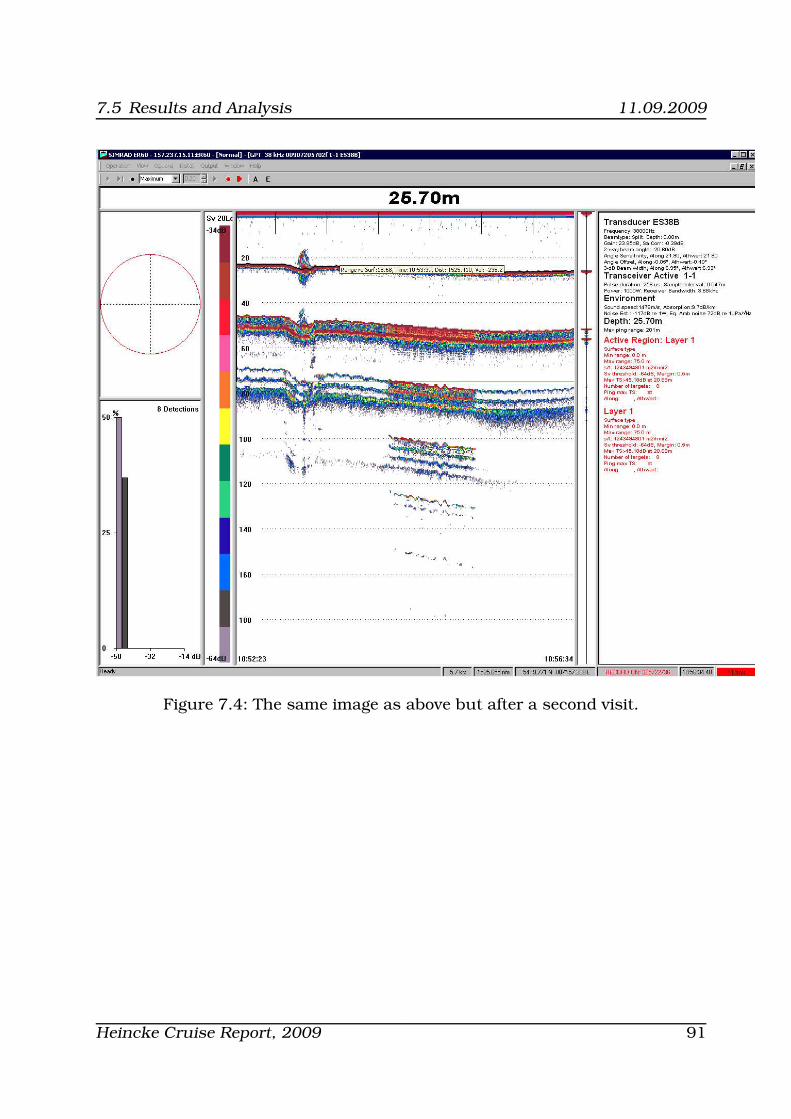
7.5 Results and Analysis 11.09.2009
Figure 7.4: The same image as above but after a second visit.
Heincke Cruise Report, 2009 91

11.09.2009 7 Echosounder
Figure 7.5: An image of the seabed showing the small underwater hillocks.
7.6 Discussion and Conclusion
The data obtained were very good as a range of frequencies were used to mapthe ocean floor. The higher frequencies have lower penetration power and areused to map shallower areas. Whereas, the lower frequencies are used to mapthe deeper areas. As, in our case a whole array of frequencies, namely 38 Khz,70 Khz, 120 KHz and 200 KHz were used and then, the best diagram regardingthe different areas were taken. So, in our case as the area was very shallow,the average depth was around 20 meters, so the best image were obtained fromthe highest frequency i.e. 200 KHz.
92 Heincke Cruise Report, 2009
7.6 Discussion and Conclusion 11.09.2009
Then, the various structures were observed on the ocean floor. After analyzingthe structures and comparing the results from the multibeam, sonar, and othersources, few ship wrecks were found. The ship wrecks make the same sortof depression as drop stones and can hence be identified, but some of thestructures could be some dropstones as well.
If a seismic energy is reflected more than once, then it’s known as a multiple.The interface depth and separation determine the additional reflections thatare time dependent. The time lag depends upon the depth of the water i.e. it’sshorter for shallow water and long time lags for deeper waters. The sea bottommultiples as in our case, can be interpreted as deeper reflections, that travelat lower velocitites compared to a true reflection from that depth. And, as canbe seen from the images provided above, it can be seen that the multiples asequal intervals, thus can be easily recognized.
Heincke Cruise Report, 2009 93

11.09.2009 8 General Discussion, Synthesis and Conclusions
8 General Discussion, Synthesis andConclusions
by Jelle Bijma & Vikram Unnithan
94 Heincke Cruise Report, 2009

11.09.2009
9 Future Work and Collaborations
by Jelle Bijma & Vikram Unnithan
Heincke Cruise Report, 2009 95

11.09.2009 10 References
10 References
Example Bibliography
96 Heincke Cruise Report, 2009

Bibliography 11.09.2009
Bibliography
[ref1] http://hyperphysics.phy-astr.gsu.edu/hbase/magnetic/magearth.html(Information on Earth’s Magnetic Field)
[ref2] http://marinemagnetics.com/ (Information on and specifications of the
MarineMagnetics Explorer magnetometer)
[ref3] http://www.marinemagnetics.com/pdf/SeaSPY_Tech_Guide.pdf (In-
formation on Proton-Spin magnetometers and the Overhauser Effect)
Heincke Cruise Report, 2009 97