Hedging Effectiveness of Energy Exchange Traded Funds
58
i Hedging Effectiveness of Energy Exchange Traded Funds Yan Gao A Thesis In The John Molson School of Business Presented in Partial Fulfillment of the Requirements for the Degree of Master of Science in Administration (Finance Option) at Concordia University Montreal, Quebec, Canada May 2012 © Yan Gao, 2012
Transcript of Hedging Effectiveness of Energy Exchange Traded Funds

i
Hedging Effectiveness of Energy Exchange Traded Funds
Yan Gao
A Thesis
In
The John Molson School of Business
Presented in Partial Fulfillment of the Requirements
for the Degree of Master of Science in Administration (Finance Option) at
Concordia University
Montreal, Quebec, Canada
May 2012
© Yan Gao, 2012

ii
CONCORDIA UNIVERSITY
School of Graduate Studies
This is to certify that the thesis prepared
By: Yan Gao
Entitled: Hedging Effectiveness of Energy Exchange Traded Funds
and submitted in partial fulfillment of the requirements for the degree of
Master of Science in Administration (Finance Option)
complies with the regulations of the University and meets the accepted standards with respect to
originality and quality.
Signed by the final examining committee:
Chair
Dr. Rahul Ravi Examiner
Dr. Ravi Mateti Examiner
Dr. Latha Shanker Supervisor
Approved by
Chair of Department or Graduate Program Director
Dr. Harjeet S. Bhabra
Dean of Faculty
Dr. Harjeet S. Bhabra
Date
May 29, 2012

iii
ABSTRACT
Hedging Effectiveness of Energy Exchange Traded Funds
Yan Gao
This thesis examines the hedging effectiveness of energy Exchange Traded Funds (ETFs).
ETFs provide small investors the opportunity to hedge against the risk of price changes in
commodities such as crude oil, instead of using commodity futures contracts to hedge,
which require a high initial margin. In this thesis, I address the hedging effectiveness of
energy ETFs in hedging against fluctuations in the price of crude oil. I apply various
models of hedging such as the minimum variance hedge ratio model (MVHR) in which
the measure of risk is the variance of the change in the value of the hedged portfolio, and
other models in which the measure of risk is the value at risk (VaR), the conditional value
at risk (CVaR) and modified value at risk (MVaR) of the hedged portfolio. I investigate
the hedging effectiveness of energy ETFs in both in-sample and out-of-sample periods.
My results indicate that energy ETFs are effective in reducing the risks associated with
fluctuation in the price of crude oil.

iv
ACKNOWLEDGEMENTS
I would like to express my deep appreciation to the following individuals:
-My supervisor Dr. Latha Shanker, who supervised and guided me from the very
beginning to the end of my thesis. Without her help and encouragement, I would never be
able to finish this thesis.
-My committee members, Dr. Rahul Ravi and Dr. Ravi Mateti, whose suggestions
helped me to improve my thesis.
-My dear parents and my dear friends, without their constant support and
encouragement, I would not finish this thesis very rapidly.

v
TABLE OF CONTENTS
Chapter I. Introduction ........................................................................................................................ Page 1
Chapter II. Literature Review ............................................................................................................... Page 6
Chapter III. Data ................................................................................................................................. Page 11
Chapter IV. Methodology ................................................................................................................... Page 20
Chapter V. Empirical Results .............................................................................................................. Page 33
Chapter VI. Conclusion and Discussion .............................................................................................. Page 45
References ......................................................................................................................................... Page 48

vi
LIST OF TABLES
Table 1: Descriptive of each ETF ...................................................................................................... Page 14
Table 2: Descriptive Statistics of returns on ETFs and crude oil ...................................................... Page 19
Table 3: In-sample comparison of Hedging Effectiveness based on OLS regression ....................... Page 33
Table 4: Comparison of hedging effectiveness based on the OLS regression for the different
categories of ETFs: in-sample period ................................................................................................ Page 34
Table 5: Out-of-sample comparison of Hedging Effectiveness using OLS regression ..................... Page 34
Table 6: Comparison of hedging effectiveness based on the OLS regression for the different
categories of ETFs: out-of-sample period .......................................................................................... Page 35
Table 7: In-sample comparison of Hedging Effectiveness based on GARCH .................................. Page 36
Table 8: Comparison of hedging effectiveness based on the GARCH model for the different
categories of ETFs: in-sample period ................................................................................................ Page 37
Table 9: Out-of-sample comparison of Hedging Effectiveness based on GARCH ........................... Page 37
Table 10: Comparison of hedging effectiveness based on the MVHR model for the different
categories of ETFs: out-of-sample period .......................................................................................... Page 38
Table 11: In-sample comparison of Hedging Effectiveness based on VaR ....................................... Page 38
Table 12: Comparison of hedging effectiveness based on the VaR model for the different
categories of ETFs: in-sample period ................................................................................................ Page 39
Table 13: Out-of-sample comparison of Hedging Effectiveness based on VaR................................ Page 40
Table 14: Comparison of hedging effectiveness based on the VaR model for the different
categories of ETFs: out-of-sample period .......................................................................................... Page 40
Table 15: In-sample comparison of Hedging Effectiveness based on CVaR .................................... Page 41
Table 16: Comparison of hedging effectiveness based on the CVaR model for the different
categories of ETFs: in-sample period ................................................................................................ Page 41
Table 17: Out-of-sample comparison of Hedging Effectiveness based on CVaR ............................. Page 42
Table 18: Comparison of hedging effectiveness based on the CVaR model for the different
categories of ETFs: out-of-sample period .......................................................................................... Page 42
Table 19: In-sample comparison of Hedging Effectiveness based on MVaR ................................... Page 43
Table 20: Comparison of hedging effectiveness based on the MVaR model for the different
categories of ETFs: in-sample period ................................................................................................ Page 44
Table 21: Out-of-sample comparison of Hedging Effectiveness based on MVaR ............................ Page 44
Table 22: Comparison of hedging effectiveness based on the MVaR model for the different
categories of ETFs: out-of-sample period .......................................................................................... Page 45

vii
LIST OF FIGURES
Figure 1: Daily price of Crude Oil from January 2005 to May 2012 .................................................. Page 2
Figure 2: Daily price of Crude Oil from January 2011 to May 2012 .................................................. Page 3
1
Chapter I. Introduction
Exchange-traded funds (ETF) are new investment vehicles that can be traded on stock
exchanges. Since they are traded like stocks, ETFs can be bought or sold at intraday
prices not necessarily at end-of-day prices as with mutual funds. According to the
descriptions of their investment strategies, ETFs hold a pool of assets such as stocks,
bonds and commodities, etc., the return on which is expected to be as close as possible to
a specific benchmark, as for example, the S&P 500 stock index.
In comparison to mutual funds, ETFs not only are cost-effective because of lower
management fees and brokerage costs but also provide investors with exposure to a broad
range of assets such as commodities and emerging market equities, both of which are
either prohibitively expensive or inaccessible. Commodity ETFs account for 10% of total
ETF assets in 2011 and have become one of the most important tools to obtain exposure
to commodity prices (Kosev and Williams, 2011). The advantage offered by commodity
ETFs is that investors can obtain exposures to commodity prices without being required
to buy and store the physical commodities.
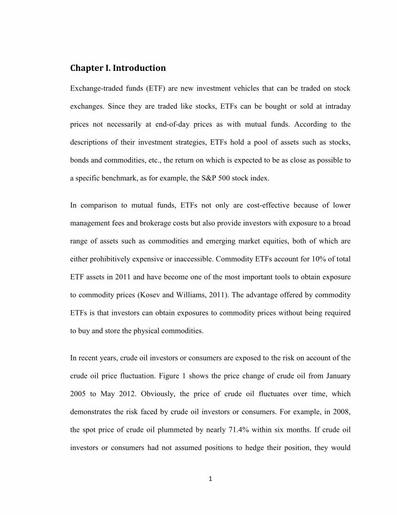
In recent years, crude oil investors or consumers are exposed to the risk on account of the
crude oil price fluctuation. Figure 1 shows the price change of crude oil from January
2005 to May 2012. Obviously, the price of crude oil fluctuates over time, which
demonstrates the risk faced by crude oil investors or consumers. For example, in 2008,
the spot price of crude oil plummeted by nearly 71.4% within six months. If crude oil
investors or consumers had not assumed positions to hedge their position, they would

2
have probably incurred huge losses. Figure 2 shows that in the recent period extending,
from January 2011 to May 2012, the price of crude oil has been volatile, fluctuating
around $ 100 per barrel. Therefore, it is necessary to hedge against crude oil price
fluctuation.
Figure 1: Daily price of Crude Oil from January 2005 to May 2012
Source: Bloomberg
$0.00
$20.00
$40.00
$60.00
$80.00
$100.00
$120.00
$140.00
$160.00
USD
per
bar
rel o
f cr
ud
e o
il
Crude Oil Price ( 2005.1- 2012.5)
Crude oil price
Date
3
Figure 2: Daily price of Crude Oil from January 2011 to May 2012
Source: Bloomberg
Historically, hedging with the use of financial instruments has been restricted to the use
of derivatives (i.e., futures, options and forwards contracts) whose pricing mechanics are
based on a complex mathematical formula. The Black and Scholes option pricing model,
which is generally used by sophisticated investors, involves complexities which may
make it difficult for small investors to use in hedging. Moreover, derivatives such as
forwards contracts are not accessible to small or individual investors since only large
institutions or companies are able to make the agreements with each other. Forwards
contracts are traded over the counter and they have to be held to maturity. In addition,
high initial margin required by futures contracts and the short time to delivery also limit
small investors from using conventional derivatives to hedge. With the advent of ETFs,
$0.00
$20.00
$40.00
$60.00
$80.00
$100.00
$120.00
20
11
-1-3
20
11
-2-3
20
11
-3-3
20
11
-4-3
20
11
-5-3
20
11
-6-3
20
11
-7-3
20
11
-8-3
20
11
-9-3
20
11
-10
-3
20
11
-11
-3
20
11
-12
-3
20
12
-1-3
20
12
-2-3
20
12
-3-3
20
12
-4-3
20
12
-5-3
USD
per
bar
rel o
f cr
ud
eo
il
Crude Oil Price ( 2011.1-2012.5)
Crude Oil Price
Date
4
however, a broad range of investor groups is able to access hedging tools since ETFs are
listed and traded as securities on stock exchanges. Commodity ETFs help farmers or
producers to hedge the price risk associated with the sale of their products and the buyers
to fix the price of their targeted products. Moreover, portfolio managers are able to adjust
hedge ratios in a short term such as every week if they use ETFs to hedge.
Recently, hedging against price fluctuation of commodities such as crude oil using
commodity ETFs is becoming more and more popular primarily due to the higher
liquidity of ETFs compared to futures contracts. Moreover, commodity ETFs allow
investors to take positions with lower entrance fees and lower holding or management
fees. In addition, commodity ETFs require a much smaller initial investment margin than
futures contracts do. For example, one crude oil futures contract on 1000 barrels of oil
requires an initial margin of around $9000 while the price of one share of US OIL ETF is
currently around $50. The lower minimum initial investment benefits small investors who
are not able to hedge with derivatives on account of the large initial investment margin
required by traditional commodity futures. Those investors can just link their future
returns to commodity prices through specific ETFs to hedge against price fluctuation of
commodities, purchasing and selling hedging components in small increments.
Although ETFs provide a convenient method for both large and small investors to hedge
against commodity price fluctuations, few studies have explored the hedging
effectiveness of commodity ETFs. Most of the previous research studies the performance
measures of ETF or the comparison of performance measures between ETF and mutual
funds. For example, Aber, Li and Can (2009) compare the tracking error of their sample
5
ETFs to that of the corresponding index mutual funds between 2000 and 2006. The
objective of this thesis is to bridge this gap. However, its scope is limited to focusing on
energy ETFs. I use data from all energy ETFs listed on US stock exchanges and London
stock exchanges with the requirement that these ETFs initiated trading before 2008.
First, the Minimum Variance Hedge Ratio (MVHR) model is applied to estimate the
optimal hedge ratios using in-sample data. Under the MVHR model, the measure of risk
is the variance of the hedged portfolio. In earlier applications of the MVHR model, the
variance of changes in the spot price of crude oil and the changes in the price of the
hedging instrument were assumed to be constant. This assumption of constant variance is
relaxed by applying a Generalized Autoregressive Conditional Heteroscedasticity
(GARCH) approach to estimate the conditional variance of the changes in the spot price
of crude oil as well as the hedging instrument and thus the optimal hedge ratio. Note that
the MVHR model focuses on the variance of the changes in the value of the hedged
portfolio as a measure of risk. In contrast, the value at risk (VaR) of a portfolio is the
maximum loss that could be expected to occur over a particular horizon with a given
confidence level. The conditional value at risk (CVaR) is the expected loss on the
portfolio, given that the loss exceeds VaR. While it is usual to assume that the changes in
the value of the portfolio follows a normal distribution in estimating VaR and CVaR,
modified value at risk (MVaR) takes into account the skewness and kurtosis of the
probability density function of the changes in the value of the portfolio. Using VaR,
CVaR and MVaR of the changes in the value of the hedged portfolio of crude oil and the
energy ETF in turn as the measure of risk, I estimate optimal hedge ratios and hedging
effectiveness by minimizing VaR, CVaR and MVaR respectively. Under the MVHR

6
model, the hedging effectiveness measure is the proportionate reduction in risk achieved
by using the hedging instrument. Similarly, I use the proportionate reduction in the VaR,
CVaR and MVaR respectively, to measure hedging effectiveness with these three
measures of risk.
This thesis is structured as follows; Chapter II presents a literature review. Chapter III
and IV describe the data and methodology, respectively. Chapter V interprets the
empirical results and Chapter VI summarizes the conclusions.
Chapter II. Literature Review
Physical Versus Synthetic ETFs and Commodity ETFs
ETFs are stock-featured funds which can be traded on stock exchanges. Basically, ETFs
can be classified into physical ETFs and synthetic ETFs. Physical ETFs’ asset allocation
is related to the components of their underlying benchmark. For example, an equity-based
ETF can hold all or part of the stocks of one underlying equity index for replicating the
benchmark. The merits of a physical replication strategy include greater transparency of
the ETF’s asset holdings and more certainty of entitlement for investors once the ETFs
are liquidated (Kosev and Williams, 2011). Synthetic ETFs refer to those ETFs which
hold derivatives such as futures, forwards and options in their portfolio. Moreover,
synthetic ETFs have lower costs as they do not need to rebalance their portfolio each time
their index is changed or reweighted. Like futures, commodity ETFs do not require the
investors to buy and store the physical commodities. The return of synthetic ETFs
consists of three parts: the change in the price of the futures contract on the commodity,
the rollover yield and the interest earned on collateral. The rollover yield refers to the

7
yield obtained by rolling over the front month futures into the next month. Interest on
collateral is produced from the cash value of the initial investment.
Most commodity ETFs in Europe are built as Exchange Traded Commodities (ETC)
(Kosev and Williams, 2011). The ETC market was initiated in 2003 with the first gold
product, Gold Bullion Securities. By 2007, the number of ETC products over the world
increased from 10 to over 80 (Biekowski, 2007). Generally speaking, ETCs are set up to
track the performance of a single commodity or to track the performance of underlying
commodity indices (i.e. energy index, agricultural products index), so they function like
ETFs. The single commodity ETC follows the spot price of one commodity whereas
index-tracking ETCs follow the performance of an underlying commodity index (London
Stock Exchange, 2009). ETCs have low correlation to equities and bonds, leading to
reduced risks without reducing returns (London Stock Exchange, 2009). Despite different
regulation and disclosure requirements, both ETFs and ETCs are listed and traded in
similar ways so that I consider ETCs in my sample as well.
Most of the previous research, however, studies the performance measures of ETF or the
comparison of performance measures between ETFs and mutual funds. Kostovetsky
(2003) claims the main differences between ETFs and index mutual funds are the
management fees, transaction fees, and taxation efficiency. Aber, Li and Can (2009)
compare the tracking error of a sample ETF to that of the index mutual funds which have
the same index as the ETF has between 2000 and 2006. They find that both ETF and the
index mutual funds correlate their corresponding indices to almost the same extent.
Rompotis (2009a) examines the performance of ETFs and index mutual funds, both of
8
which are sponsored by the same fund manager such as Vanguard, in order to examine
the interfamily competition. He finds that ETFs and index mutual funds have similar
returns, volatility and low tracking errors. Besides, they both underperform their
benchmark because of expenses and fees.
Models of Hedging
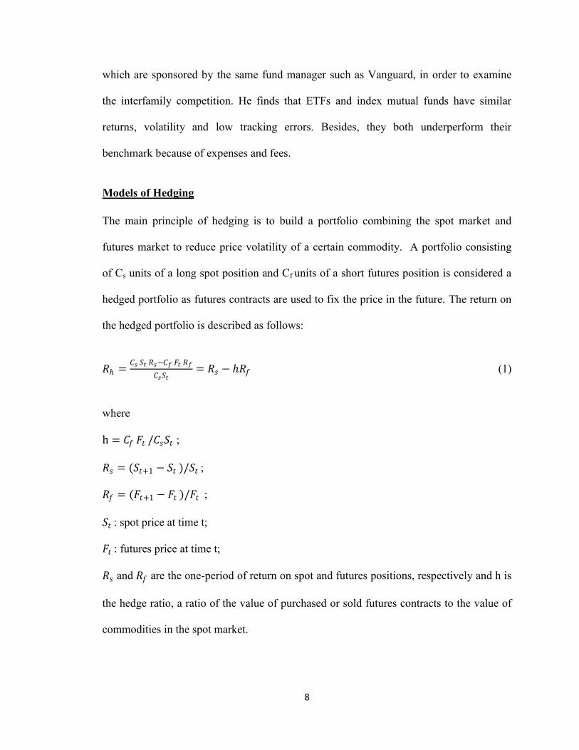
The main principle of hedging is to build a portfolio combining the spot market and
futures market to reduce price volatility of a certain commodity. A portfolio consisting
of Cs units of a long spot position and Cf units of a short futures position is considered a
hedged portfolio as futures contracts are used to fix the price in the future. The return on
the hedged portfolio is described as follows:
𝑅 =𝐶𝑠 𝑆𝑡 𝑅𝑠−𝐶𝑓 𝐹𝑡 𝑅𝑓
𝐶𝑠𝑆𝑡= 𝑅𝑠 − 𝑅𝑓 (1)
where
h = 𝐶𝑓 𝐹𝑡 /𝐶𝑠𝑆𝑡 ;
𝑅𝑠 = (𝑆𝑡+1 − 𝑆𝑡 )/𝑆𝑡 ;
𝑅𝑓 = (𝐹𝑡+1 − 𝐹𝑡 )/𝐹𝑡 ;
𝑆𝑡 : spot price at time t;
𝐹𝑡 : futures price at time t;
𝑅𝑠 and 𝑅𝑓 are the one-period of return on spot and futures positions, respectively and h is
the hedge ratio, a ratio of the value of purchased or sold futures contracts to the value of
commodities in the spot market.
9
The earliest model which applied portfolio theory to estimate the optimal hedge ratio is
the minimum variance hedge ratio (MVHR) (Ederington, 1979; Johnson, 1960; Myers,
Thompson, 1989) model. The MVHR model is easy to understand and apply in practice.
It, however, ignores the expected return of the hedged portfolio and therefore it is not
consistent with the mean-variance framework unless investors focus only on risk or
unless the price of the hedging instrument (energy ETFs price in our case) strictly follows
a martingale process (Chen, et al., 2003). In earlier applications of the MVHR model, the
hedge ratio is a static one, which means that the hedge ratio would not be revised during
the hedging period. However, new information or news that arrives in the market may
affect hedging strategies. Accordingly, the optimal hedge ratio should change over time.
ARCH and GARCH models, which are based on conditional distributions, are used to
estimate dynamic time-varying hedge ratios. Baillie and Myers (1991) use daily data to
examine six different commodities, beef, coffee, corn, cotton, gold and soybeans over
two futures contract periods and find that a dynamic hedging strategy outperforms the
static hedging strategy. Park and Switzer (1995) examine three stock index futures
contracts in North America, comparing hedging performances of both stationary models
based on Ordinary Least Squares (OLS) regression, OLS with cointegration and dynamic
models such as bivariate GARCH. They conclude that the dynamic hedging strategy
improves hedging performance over that of the traditional static hedging strategies.
Cao, Harris and Shen (2010) point out that MVHR is appropriate with respect to risk
reduction only when investors have quadratic utility or when returns are elliptically
distributed. When the above two assumption is not satisfied, variance is not the optimal
measure of risk since it ignores the skewness and kurtosis of the return distribution.

10
Accordingly, new measures of risk emerge. Some studies have revealed that portfolio
managers care about losses more than gains. Bawa (1975) proposes lower partial
moments to measure downside risks. Thereafter, a number of models that measure
downside risk have been proposed. For example, Lien et al. (2001) and Lien & Tse (2000)
find the optimum hedge ratio by minimizing the hedged portfolio’s generalized
semivariance (GSV), which also considers stochastic dominance. These authors find that
traditional mean variance hedging strategies are not efficient if portfolio managers only
care about downside risk.
The Value at Risk approach was first introduced by J. P. Morgan in the 1990s and
adopted by the Basle Committee to determine the minimum regulatory capital of banks
(Alexander, Baptista, 2006). VaR now has been widely used as a risk management tool
by many financial institutions. Referring to the definition of VaR (Jorion, 2000), Hung,
Chiu and Lee(2006) provide an alternative hedging method by using a zero- VaR
approach to measure downside risks of the hedged portfolio and they also derive a zero-
VaR hedge ratio. After deriving the hedge ratio based on zero-VaR approach, they
compare the zero-VaR hedge ratio to the MVHR hedge ratio. They conclude that as the
risk-aversion level of investors increases, the zero-VaR hedge ratio converges to the
MVHR, while if investors only care about downside risk, the zero-VaR hedge ratio may
be completely different from the MVHR. In that case, the hedging strategy that
minimizes the variance of the hedged portfolio becomes inappropriate. Cao, Harris and
Shen (2010) derive the minimum-VaR and minimum-CVaR hedge ratios by using a
semi-parametric method based on the Cornish-Fisher expansion. The new approach is
applied to four equity index positions associated with equity index futures. They find that

11
the semi-parametric method of estimating the minimum-VaR and minimum-CVaR is
superior to the minimum variance approach and results in greater reduction in VaR and
CVaR. Favre and Galeano (2002) modify the VaR approach, take into account the
skewness and kurtosis of the return distribution and propose a new approach called the
Modified Value at Risk (MVaR) approach to calculate the optimal hedge ratio by
minimizing the MVaR at a given confidence level. The advantage of the MVaR
approach over the VaR approach is that it is not based on any distribution assumption,
therefore non-normal distribution of portfolio returns will not affect the hedging
performance. They find that compared to the benefits of using the risk measures of VaR
and the variance, the benefits of using the risk measure of MVaR would be higher if the
portfolio has negative skewness or a positive kurtosis.
Chapter III. Data
Daily closing prices of ETFs and crude oil are obtained from Bloomberg. The daily total
returns for each ETF are calculated as the percentage change in daily closing prices. The
sample period covers the period from the date of inception of each ETF to January 11,
2012. For example, ProShares Ultra Oil & Gas Fund (DIG) started trading in 2007 while
PowerShares Dynamic Oil & Gas Service Portfolio Fund (PXJ) commenced trading in
2006. I pool all of the energy ETFs together to construct the panel data. In order to have a
long enough period time of data, only those ETFs that started trading at least from 2008
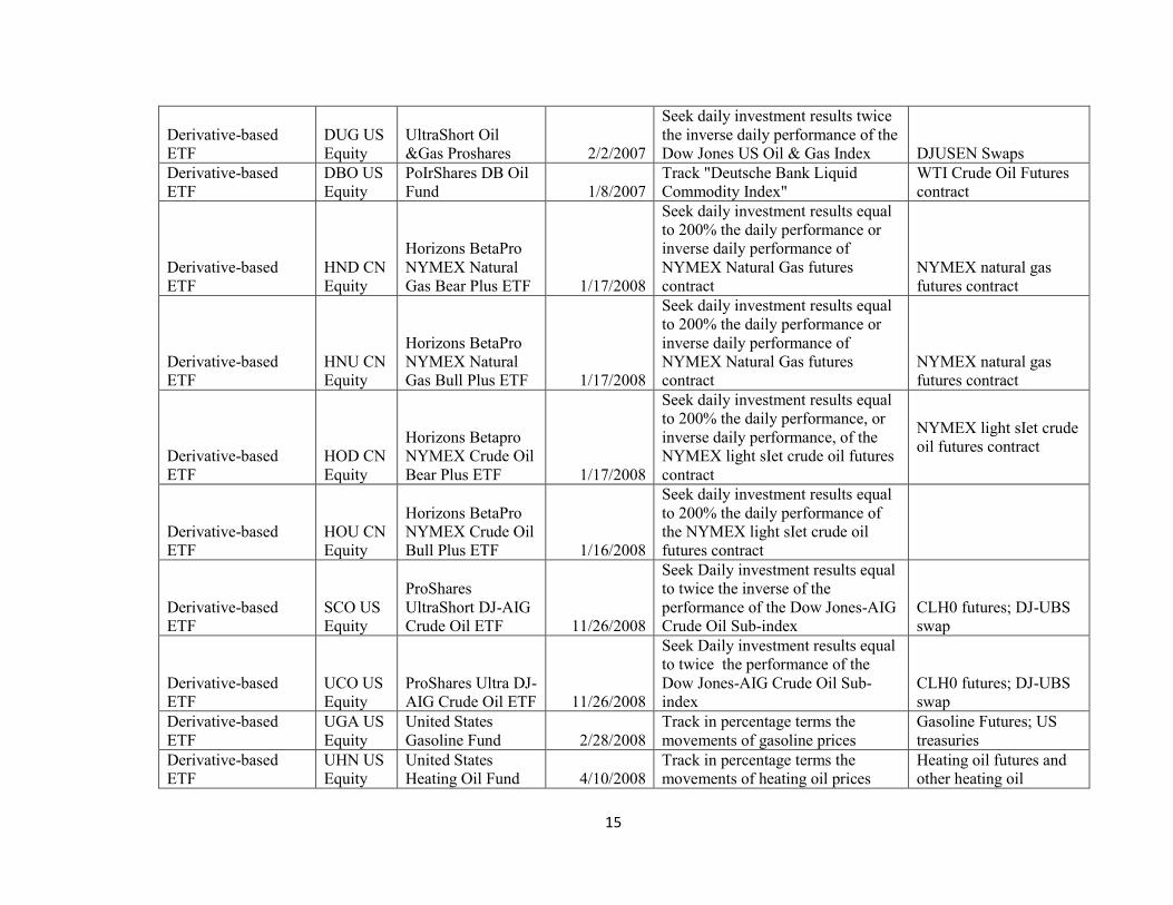
are selected. Table 1 shows the list of the ETFs used in this study along with information
on their inception date, their investment strategies and their main holdings. Based on the
ETFs’ investment strategy and top holdings, I categorize these ETFs into four categories.

12
The first category, Stock-based ETFs, includes energy index ETFs, which attempt to
track, before fees and expenses, the daily performance of some energy indices such as
Dow Jones US Oil and Gas index. Basically, the portfolios of ETFs in this category
mainly consist of energy corporations’ stocks. The second category, Derivative-based
ETFs, includes synthetic ETFs, the asset allocation of which includes crude oil or natural
gas futures contracts or swaps. The percentage change in price of these ETFs is intended
to reflect the percentage changes in the price of crude oil, heating oil or other energy
commodity which is tracked by the changes in the price of the futures contract. The third
category, Derivative-based ETCs, includes ETCs that hold futures contracts or forwards
just as Derivative-based ETFs do. However, these ETCs are traded on the London Stock
Exchange. I consider these ETCs separately since differences in the rules and regulations
that govern ETFs in the U.S. and the U.K. may affect their hedging performance. The
fourth category, Single-commodity ETFs, consists of ETFs on a single commodity such
as crude oil or natural gas. Stock-based ETFs contain 8 ETFs, Derivative-based ETFs
contain 13 ETFs, Derivative-based ETCs contain 8 ETCs and Single-commodity ETFs
contain 19 ETFs. Finally, the daily return on an equal weighted portfolio of the 48 ETFs
included in the study is also calculated for the sample period.
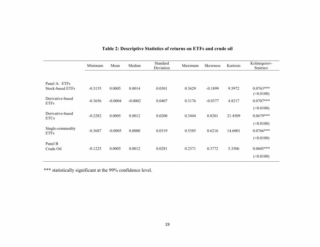
Table 2 provides descriptive statistics of the returns on the 48 ETFs as well as returns on
crude oil. These statistics include the minimum, the maximum, and the first four
moments of the return distribution (mean, standard deviation, skewness and kurtosis).
Table 2 shows that the mean returns of these four categories of energy ETFs are lower
than the mean return of the spot price of crude oil. Except for Derivative-based ETCs,
whose portfolios include futures and swaps etc., the standard deviation of the returns of
13
the other ETF categories is higher than the standard deviation of returns on crude oil.
Derivative-based ETCs have the highest mean return and the lowest standard deviation,
which suggests that the Derivative-based ETCs have the lowest risks. The positive
median and skewness of Derivative-based ETCs reveals that the probability of positive
return is higher than for the other three categories.
As it is shown in Table 2, the skewness and kurtosis of both energy ETFs and spot crude
oil are significantly different from 0 and 3, respectively. The Kolmogorov-Smirnov test is
applied to test for normality of the returns on the ETFs and on crude oil. The p-values of
the Kolmogorov-Smirnov statistics of the four categories and of crude oil are all below
0.01, which suggests that the assumption of normally distributed returns is rejected at the
99% confidence level. These deviations from normally distributed returns imply that the
Modified VaR model should be a more appropriate specification.

14
Table 1: Descriptive of each ETF
Type Ticker Name
Inception
Date Strategies Top Holdings
Stock-based ETF
DIG US
Equity
ProShares Ultra Oil
and Gas 2/2/2007
Seek daily investment results twice
the daily performance of the Dow
Jones US Oil & Gas Index
Exxon Mobil; Chevron;
ConocoPhillips
Stock-based ETF
ENY US
Equity
Claymore/SWM
Canadian Energy
Income Index ETF 7/5/2007
Track the Sustainable Canadian
Energy Income Index
Canadian Oil Sands
Trust, Baytex Energy
Trust; Suncor Energy
Inc.
Stock-based ETF
FCG US
Equity
First Trust ISE-
Revere Natual Gas
Index Fund 5/16/2007
Track "ISE-Revere Natural Gas
IndexTM"
PetroQuest Energy, Inc.;
Pioneer Natural
Resources Company;
Forest Oil Corporation
Stock-based ETF
IEO US
Equity
Ishares Dow Jones
U.S. Oil & Gas
Exploration &
Production Index
Fund 5/8/2006
Track "Dow Jones US Select Oil
Exploration & Production Index"
Occidental Peroleum
Corp; Apache Corp;
Anadarko Petroleum
Corp
Stock-based ETF
IEZ US
Equity
Ishares Dow Jones
U.S. Oil Equipment
Index 5/8/2006
Track"Dow Jones US Select Oil
Equipment & Service Index"
Schlumberger LTD;
Halliburton Co; National
OilIll Varco Inc
Stock-based ETF
PXJ US
Equity
PoIrshares
Dynamic Oil&Gas
Service Portfolio
ETF 10/27/2005
Track" Oil & Gas Services
Intellidex index"
Halliburton Co.;
National OilIll Varco
Inc.; Schlumberger Ltd.
Stock-based ETF
XES US
Equity
SPDR S&P Oil &
Gas Equipment &
Services 6/23/2006
Track"S&P Oil & Gas Equipment
& Services Select Industry Index"
Schlumberger Ltd. ;
Halliburton Co; National
OilIll Varco Inc.
Stock-based ETF
XOP US
Equity
SPDR S&P Oil &
Gas Exploration &
Production ETF 6/23/2006
Track"S&P Oil & Gas Exploration
& Production Select Industry Index"
Exxon Mobil Corp;
Chevron Corp New;
Conocophillips
Derivative-based
ETF
DDG US
Equity
First Trust ISE-
Revere Natual Gas
Index Fund 6/19/2008
Seek daily investment results
inverse of the daily performance of
the Dow Jones US Oil & Gas Index DJUSEN Swaps
15
Derivative-based
ETF
DUG US
Equity
UltraShort Oil
&Gas Proshares 2/2/2007
Seek daily investment results twice
the inverse daily performance of the
Dow Jones US Oil & Gas Index DJUSEN Swaps
Derivative-based
ETF
DBO US
Equity
PoIrShares DB Oil
Fund 1/8/2007
Track "Deutsche Bank Liquid
Commodity Index"
WTI Crude Oil Futures
contract
Derivative-based
ETF
HND CN
Equity
Horizons BetaPro
NYMEX Natural
Gas Bear Plus ETF 1/17/2008
Seek daily investment results equal
to 200% the daily performance or
inverse daily performance of
NYMEX Natural Gas futures
contract
NYMEX natural gas
futures contract
Derivative-based
ETF
HNU CN
Equity
Horizons BetaPro
NYMEX Natural
Gas Bull Plus ETF 1/17/2008
Seek daily investment results equal
to 200% the daily performance or
inverse daily performance of
NYMEX Natural Gas futures
contract
NYMEX natural gas
futures contract
Derivative-based
ETF
HOD CN
Equity
Horizons Betapro
NYMEX Crude Oil
Bear Plus ETF 1/17/2008
Seek daily investment results equal
to 200% the daily performance, or
inverse daily performance, of the
NYMEX light sIet crude oil futures
contract
NYMEX light sIet crude
oil futures contract
Derivative-based
ETF
HOU CN
Equity
Horizons BetaPro
NYMEX Crude Oil
Bull Plus ETF 1/16/2008
Seek daily investment results equal
to 200% the daily performance of
the NYMEX light sIet crude oil
futures contract
Derivative-based
ETF
SCO US
Equity
ProShares
UltraShort DJ-AIG
Crude Oil ETF 11/26/2008
Seek Daily investment results equal
to twice the inverse of the
performance of the Dow Jones-AIG
Crude Oil Sub-index
CLH0 futures; DJ-UBS
swap
Derivative-based
ETF
UCO US
Equity
ProShares Ultra DJ-
AIG Crude Oil ETF 11/26/2008
Seek Daily investment results equal
to twice the performance of the
Dow Jones-AIG Crude Oil Sub-
index
CLH0 futures; DJ-UBS
swap
Derivative-based
ETF
UGA US
Equity
United States
Gasoline Fund 2/28/2008
Track in percentage terms the
movements of gasoline prices
Gasoline Futures; US
treasuries
Derivative-based
ETF
UHN US
Equity
United States
Heating Oil Fund 4/10/2008
Track in percentage terms the
movements of heating oil prices
Heating oil futures and
other heating oil

16
interests; US treasuries
Derivative-based
ETF
UNG US
Equity
United States
Natural Gas Fund 4/19/2007
Track in percentage terms the
movements of natural gas prices
Derivative-based
ETF
USO US
Equity
United States Oil
Fund 4/11/2006
Track the movements of light, sIet
crude oil
oil futures and other oil
interests; US treasuries
Derivative-based
ETC
OILB LN
Equity
ETFS Brent Oil
ETF 7/29/2005
Track ICE futures brent contracts
with an average maturity of one
month ETFS brent 1 month
Derivative-based
ETC
OILW
LN
Equity ETFS WTI Oil ETF 5/12/2006
Track NYMEX WTI oil contracts
with an average maturity of two
month ETFS brent 2 months
Derivative-based
ETC
OSB1
LN
Equity
ETFS Brent 1yr
ETF 8/16/2007
Track December ICE Futures Brent
oil contracts with an average
maturity of one year ETS Brent 1 year
Derivative-based
ETC
OSB2
LN
Equity
ETFS Brent 2yr
ETF 8/15/2007
Track December ICE Futures Brent
oil contracts with an average
maturity of two years ETS Brent 2 year
Derivative-based
ETC
OSB3
LN
Equity
ETFS Brent 3yr
ETF 8/17/2007
Track December ICE Futures Brent
oil contracts with an average
maturity of three years ETS Brent 3 year
Derivative-based
ETC
OSW1
LN
Equity ETFS WTI 1yr ETF 8/16/2007
Track NYMEX WTI oil contracts
with an average maturity of one
year ETFS WTI 1 year
Derivative-based
ETC
OSW2
LN
Equity ETFS WTI 2yr ETF 8/16/2007
Track NYMEX WTI oil contracts
with an average maturity of two
years ETFS WTI 2 year2
Derivative-based
ETC
OSW3
LN
Equity ETFS WTI 3yr ETF 8/16/2007
Track NYMEX WTI oil contracts
with an average maturity of three
years ETFS WTI 3 year3
Single-commodity
ETF
AIGO
LN
Equity
ETFS Petroleum
ETF 9/29/2006
Track the DJ-AIG Petroleum Sub-
Index
Crude oil(WTI);
Unleaded Gasoline;
Heating Oil
Single-commodity
ETF
CRUD
LN
Equity
ETFS Crude Oil
ETF 9/29/2006
Track the DJ-AIG Crude Oil Sub-
Index Crude oil(WTI)

17
Single-commodity
ETF
FPET LN
Equity
ETFS Forward
Petroleum ETF 10/12/2007
Track the DJ-UBS Petroleum Sub-
index
Crude oil(WTI);
Unleaded Gasoline;
Heating Oil
Single-commodity
ETF
HEAF
LN
Equity
ETFS Forward
Heating Oil ETF 11/30/2007
Track the DJ-UBS Heating Oil Sub-
index Heating oil
Single-commodity
ETF
HEAT
LN
Equity
ETFS Heating Oil
ETF 9/29/2006
Track the DJ-UBS Heating Oil Sub-
index Heating oil
Single-commodity
ETF
LGAS
LN
Equity
ETFS Leveraged
Gasoline ETF 3/12/2008
Seek daily investment results twice
the daily performance of the DJ-
UBS Gasoline Sub-index Unleaded Gasoline
Single-commodity
ETF
LHEA
PZ
Equity
ETFS Leveraged
Heating Oil ETF 9/23/2008
Seek daily investment results twice
the daily performance of the DJ-
UBS Heating Oil Sub-index Heating Oil
Single-commodity
ETF
LNGA
LN
Equity
ETFS Leveraged
Natural Gas ETF 3/12/2008
Seek daily investment results twice
the daily performance of the DJ-
UBS Natural Gas Sub-index Natural Gas
Single-commodity
ETF
LOIL LN
Equity
ETFS Leveraged
Crude Oil ETF 3/12/2008
Seek daily investment results twice
the daily performance of the DJ-
UBS Crude Oil Sub-index Crude Oil (WTI)
Single-commodity
ETF
LPET LN
Equity
ETFS Leveraged
Petroleum ETF 3/12/2008
Seek daily investment results twice
the daily performance of the DJ-
UBS Petroleum Sub-index
Crude oil(WTI);
Unleaded Gasoline;
Heating Oil
Single-commodity
ETF
NGAF
LN
Equity
ETFS Forward
Natual Gas ETF 11/30/2007
Track the DJ-AIG Natural Gas sub-
index Natural Gas
Single-commodity
ETF
NGAS
LN
Equity
ETFS Natural Gas
ETF 9/29/2006
Track the DJ-AIG Natural Gas sub-
index Natural Gas
Single-commodity
ETF
NGSP
LN
Equity
ETFS Natural Gas
Sterling ETF 10/30/2007
Track the DJ-AIG Natural Gas sub-
index Natural Gas
Single-commodity
ETF
SGAS
LN
Equity
ETFS Short
Gasoline ETF 2/25/2008
Seek daily investment results
inverse the daily performance of the
DJ-UBS Gasoline Sub-index Unleaded Gasoline

18
Single-commodity
ETF
SHEA
LN
Equity
ETFS Short
Heating Oil ETF 2/25/2008
Seek daily investment results
inverse the daily performance of the
DJ-UBS Heating Oil Sub-index Heating Oil
Single-commodity
ETF
SNGA
LN
Equity
ETFS Short Natural
Gas ETF 2/25/2008
Seek daily investment results
inverse the daily performance of the
DJ-UBS Natural Gas Sub-index Natural Gas
Single-commodity
ETF
SOIL LN
Equity
ETFS Short Crude
Oil ETF 2/25/2008
Seek daily investment results
inverse the daily performance of the
DJ-UBS Crude Oil Sub-index Crude Oil(WTI)
Single-commodity
ETF
SPET LN
Equity
ETFS Short
Petroleum ETF 2/25/2008
Seek daily investment results
inverse the daily performance of the
DJ-UBS Petroleum Sub-index
Crude oil(WTI);
Unleaded Gasoline;
Heating Oil
Single-commodity
ETF
UGAS
LN
Equity
ETFS Gasoline
ETF 9/29/2006
Track the DJ-UBS Unleaded
Gasoline Sub-index Unleaded Gasoline
19
Table 2: Descriptive Statistics of returns on ETFs and crude oil
Minimum Mean Median
Standard
Deviation Maximum Skewness Kurtosis
Kolmogorov-
Smirnov
Panel A: ETFs
Stock-based ETFs -0.3155 0.0005 0.0014 0.0301 0.3629 -0.1899 9.5972 0.0763***
(<0.0100)
Derivative-based
ETFs -0.3656 -0.0004 -0.0002 0.0407 0.3176 -0.0377 4.8217 0.0707***
(<0.0100)
Derivative-based
ETCs -0.2282 0.0005 0.0012 0.0200 0.3444 0.8201 21.4509 0.0679***
(<0.0100)
Single-commodity
ETFs -0.3687 -0.0005 0.0000 0.0319 0.5385 0.6216 14.6001 0.0766***
(<0.0100)
Panel B
Crude Oil -0.1225 0.0005 0.0012 0.0281 0.2371 0.3772 5.3506 0.0605***
(<0.0100)
*** statistically significant at the 99% confidence level.

20
Chapter IV. Methodology
I describe previous research in which spot price fluctuations were hedged using futures
contracts. I apply this research to determine the hedging effectiveness of energy ETFs in
hedging crude oil fluctuations. In this application, the energy ETF is the hedging
instrument and takes the place of the futures contract in previous research. Accordingly,
in this application of these models, the change in the futures price is replaced by the
change in the price of the ETFs which are used to hedge.
Minimum Variance Hedge Ratio Model
Ederington (1978) derives the MVHR by minimizing the portfolio’s risk, which is
proxied by the variance of the portfolio’s returns. The objective function is described as
follows:
𝑀𝑖𝑛𝑖𝑚𝑖𝑧𝑒 𝑉𝑎𝑟 𝑉 = 𝑣𝑎𝑟(∆𝑆 − ∆𝐹)
= σ∆s2 + 2σ∆f
2 − 2hσ∆s,∆f (2)
with respect to h
where
∆ 𝑆: change in the spot price;
∆ 𝐹: change in the futures price;
σ∆s2 : variance of the change in the spot price;
σ∆f2 : variance in the change in the futures price;
σ∆s,∆f: covariance between the change in the spot price and the change in the futures price;
h: hedge ratio, which is the number of units of futures for each unit of the spot
commodity.
21
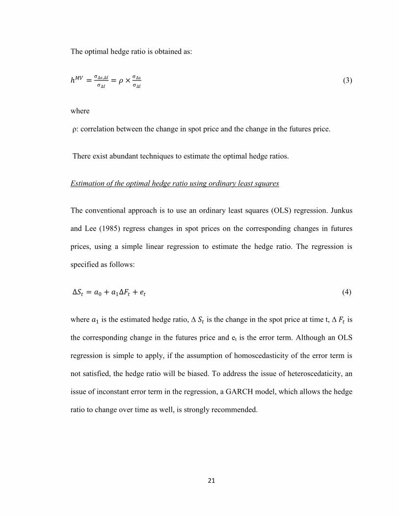
The optimal hedge ratio is obtained as:
𝑀𝑉 =σ∆s ,∆f
σ∆f= 𝜌 ×
σ∆s
σ∆f (3)
where
ρ: correlation between the change in spot price and the change in the futures price.
There exist abundant techniques to estimate the optimal hedge ratios.
Estimation of the optimal hedge ratio using ordinary least squares
The conventional approach is to use an ordinary least squares (OLS) regression. Junkus
and Lee (1985) regress changes in spot prices on the corresponding changes in futures
prices, using a simple linear regression to estimate the hedge ratio. The regression is
specified as follows:
∆𝑆𝑡 = 𝑎0 + 𝑎1∆𝐹𝑡 + 𝑒𝑡 (4)
where 𝑎1 is the estimated hedge ratio, ∆ 𝑆𝑡 is the change in the spot price at time t, ∆ 𝐹𝑡 is
the corresponding change in the futures price and et is the error term. Although an OLS
regression is simple to apply, if the assumption of homoscedasticity of the error term is
not satisfied, the hedge ratio will be biased. To address the issue of heteroscedaticity, an
issue of inconstant error term in the regression, a GARCH model, which allows the hedge
ratio to change over time as well, is strongly recommended.
22
Estimation of the optimal hedge ratio using GARCH
As new information arrives in the market, the variance of spot and futures prices could
change. Therefore, hedge ratios would change over time.
The GARCH model mainly includes five equations. The first two equations capture the
conditional means of the distribution of spot price changes and futures price changes. The
other three equations account for time-varying variances of spot price changes, variances
of futures price changes and the covariance between spot and futures price changes.
Bollerslev (1986) first proposed the GARCH(1,1) model, which was applied by Baillie
and Bollerslev(1990) to estimate the joint distribution of spot and futures prices for six
commodities, beef, coffee, corn, cotton, gold and soybeans.
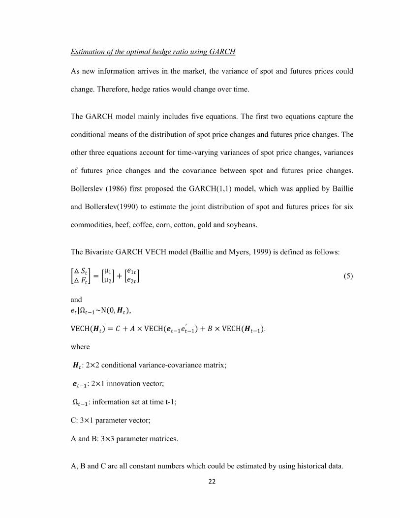
The Bivariate GARCH VECH model (Baillie and Myers, 1999) is defined as follows:
𝑆𝑡
𝐹𝑡 =
µ1
µ2 +
𝑒1𝑡
𝑒2𝑡 (5)
and
𝑒𝑡|Ω𝑡−1~N(0, 𝑯𝑡),
VECH(𝑯𝑡) = 𝐶 + 𝐴 × VECH(𝒆𝑡−1𝑒𝑡−1′ ) + 𝐵 × VECH(𝑯𝑡−1).
where
𝑯𝑡 : 2×2 conditional variance-covariance matrix;
𝒆𝑡−1: 2×1 innovation vector;
Ω𝑡−1: information set at time t-1;
C: 3×1 parameter vector;
A and B: 3×3 parameter matrices.
A, B and C are all constant numbers which could be estimated by using historical data.
23
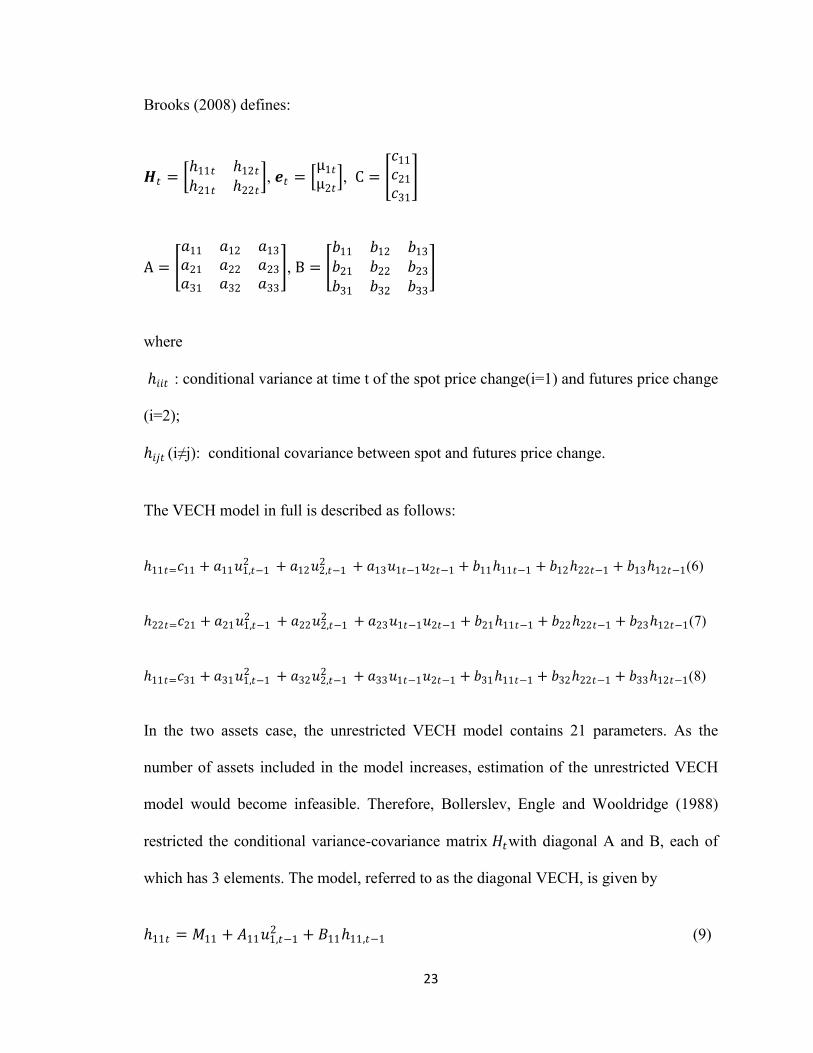
Brooks (2008) defines:
𝑯𝑡 = 11𝑡 12𝑡
21𝑡 22𝑡 , 𝒆𝑡 =
µ1𝑡
µ2𝑡 , C =
𝑐11
𝑐21
𝑐31
A =
𝑎11 𝑎12 𝑎13
𝑎21 𝑎22 𝑎23
𝑎31 𝑎32 𝑎33
, B =
𝑏11 𝑏12 𝑏13
𝑏21 𝑏22 𝑏23
𝑏31 𝑏32 𝑏33
where
𝑖𝑖𝑡 : conditional variance at time t of the spot price change(i=1) and futures price change
(i=2);
𝑖𝑗𝑡 (i≠j): conditional covariance between spot and futures price change.
The VECH model in full is described as follows:
11𝑡=𝑐11 + 𝑎11𝑢1,𝑡−1 2 + 𝑎12𝑢2,𝑡−1
2 + 𝑎13𝑢1𝑡−1𝑢2𝑡−1 + 𝑏1111𝑡−1 + 𝑏1222𝑡−1 + 𝑏1312𝑡−1(6)
22𝑡=𝑐21 + 𝑎21𝑢1,𝑡−1 2 + 𝑎22𝑢2,𝑡−1
2 + 𝑎23𝑢1𝑡−1𝑢2𝑡−1 + 𝑏2111𝑡−1 + 𝑏2222𝑡−1 + 𝑏2312𝑡−1(7)
11𝑡=𝑐31 + 𝑎31𝑢1,𝑡−1 2 + 𝑎32𝑢2,𝑡−1
2 + 𝑎33𝑢1𝑡−1𝑢2𝑡−1 + 𝑏3111𝑡−1 + 𝑏3222𝑡−1 + 𝑏3312𝑡−1(8)
In the two assets case, the unrestricted VECH model contains 21 parameters. As the
number of assets included in the model increases, estimation of the unrestricted VECH
model would become infeasible. Therefore, Bollerslev, Engle and Wooldridge (1988)
restricted the conditional variance-covariance matrix 𝐻𝑡with diagonal A and B, each of
which has 3 elements. The model, referred to as the diagonal VECH, is given by
11𝑡 = 𝑀11 + 𝐴11𝑢1,𝑡−12 + 𝐵1111,𝑡−1 (9)
24
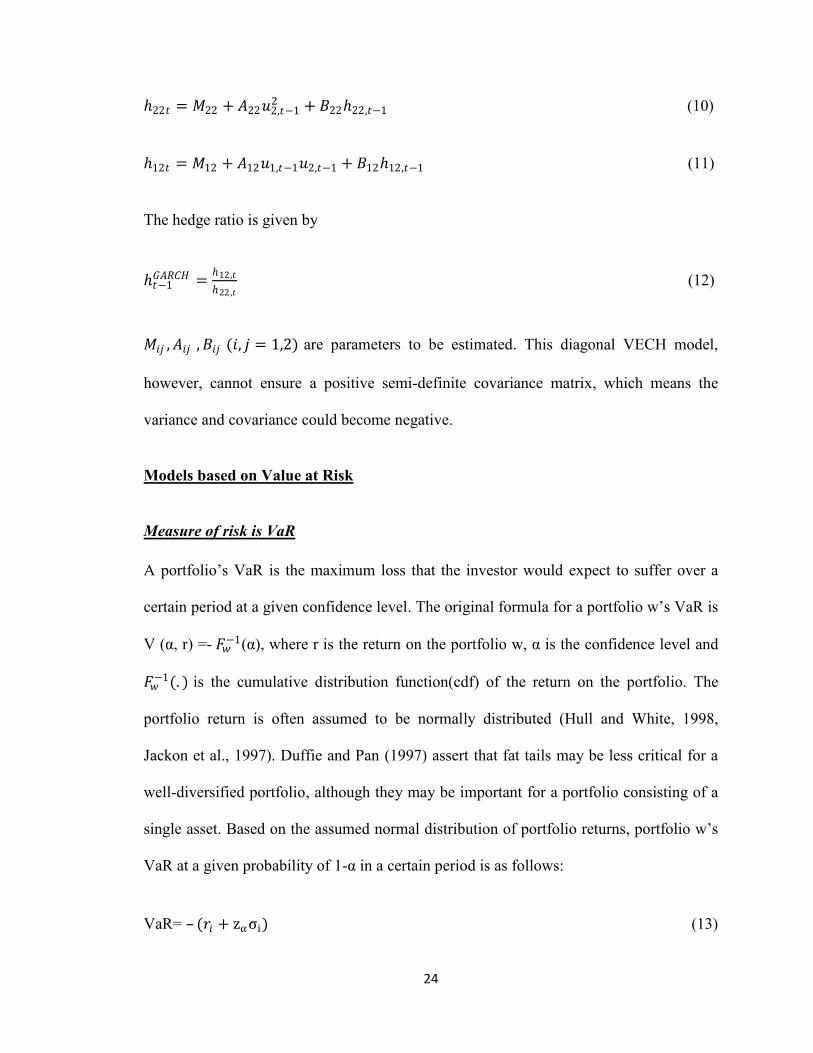
22𝑡 = 𝑀22 + 𝐴22𝑢2,𝑡−12 + 𝐵2222,𝑡−1 (10)
12𝑡 = 𝑀12 + 𝐴12𝑢1,𝑡−1𝑢2,𝑡−1 + 𝐵1212,𝑡−1 (11)
The hedge ratio is given by
𝑡−1𝐺𝐴𝑅𝐶𝐻 =
12,𝑡
22,𝑡 (12)
𝑀𝑖𝑗 , 𝐴𝑖𝑗 , 𝐵𝑖𝑗 (𝑖, 𝑗 = 1,2) are parameters to be estimated. This diagonal VECH model,
however, cannot ensure a positive semi-definite covariance matrix, which means the
variance and covariance could become negative.
Models based on Value at Risk
Measure of risk is VaR
A portfolio’s VaR is the maximum loss that the investor would expect to suffer over a
certain period at a given confidence level. The original formula for a portfolio w’s VaR is
V (α, r) =- 𝐹𝑤−1(α), where r is the return on the portfolio w, α is the confidence level and
𝐹𝑤−1(. ) is the cumulative distribution function(cdf) of the return on the portfolio. The
portfolio return is often assumed to be normally distributed (Hull and White, 1998,
Jackon et al., 1997). Duffie and Pan (1997) assert that fat tails may be less critical for a
well-diversified portfolio, although they may be important for a portfolio consisting of a
single asset. Based on the assumed normal distribution of portfolio returns, portfolio w’s
VaR at a given probability of 1-α in a certain period is as follows:
VaR= – (𝑟𝑖 + zασi) (13)

25
where
zα : αth percentile of the standard normal distribution;
𝑟𝑖 : return of the portfolio;
σi: standard deviation of the portfolio return.
α is the confidence level, which can be considered as the risk aversion parameter. For
example, if the portfolio managers prefer to take more risks, a lower confidence level can
be chosen. On the other hand, a higher confidence level can be used if the portfolio
managers are more risk averse.
I need to minimize VaR to find the optimal hedge ratios. Therefore, the objective
function is represented as follows:
Minimize 𝑉𝑎𝑅(𝑟) = −( E(𝑟) + zασh) (14)
with respect to h
where E(𝑟)=E(𝑟𝑜𝑖𝑙 ) − hE(𝑟𝐸𝑇𝐹)
𝑉𝑎𝑅 𝑟 : Value at Risk of the hedged portfolio;
E(𝑟): expected return of the hedged portfolio;
E(𝑟𝑜𝑖𝑙 ): expected return of crude oil;
E(𝑟𝐸𝑇𝐹): expected return of the ETF;
σh : standard deviation of the return on the hedged portfolio;
h: hedge ratio.
zα : αth percentile of the standard normal distribution.
26
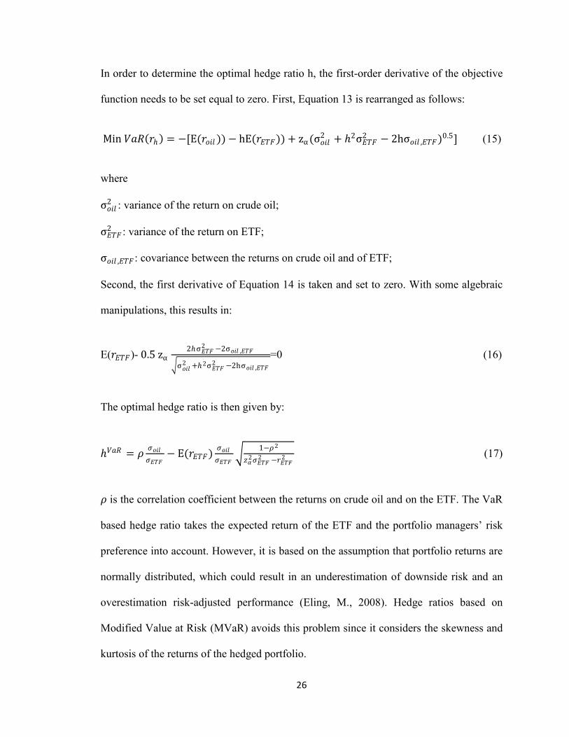
In order to determine the optimal hedge ratio h, the first-order derivative of the objective
function needs to be set equal to zero. First, Equation 13 is rearranged as follows:
Min 𝑉𝑎𝑅 𝑟 = −[E(𝑟𝑜𝑖𝑙 )) − hE(𝑟𝐸𝑇𝐹)) + zα(σ𝑜𝑖𝑙2 + 2σ𝐸𝑇𝐹
2 − 2hσ𝑜𝑖𝑙 ,𝐸𝑇𝐹)0.5] (15)
where
σ𝑜𝑖𝑙2 : variance of the return on crude oil;
σ𝐸𝑇𝐹2 : variance of the return on ETF;
σ𝑜𝑖𝑙 ,𝐸𝑇𝐹 : covariance between the returns on crude oil and of ETF;
Second, the first derivative of Equation 14 is taken and set to zero. With some algebraic
manipulations, this results in:
E(𝑟𝐸𝑇𝐹)- 0.5 zα 2σ𝐸𝑇𝐹
2 −2σ𝑜𝑖𝑙 ,𝐸𝑇𝐹
σ𝑜𝑖𝑙2 +2σ𝐸𝑇𝐹
2 −2hσ𝑜𝑖𝑙 ,𝐸𝑇𝐹
=0 (16)
The optimal hedge ratio is then given by:
𝑉𝑎𝑅 = 𝜌𝜍𝑜𝑖𝑙
𝜍𝐸𝑇𝐹− E(𝑟𝐸𝑇𝐹)
𝜍𝑜𝑖𝑙
𝜍𝐸𝑇𝐹
1−𝜌2
𝑧𝛼2𝜍𝐸𝑇𝐹
2 −𝑟𝐸𝑇𝐹2 (17)
𝜌 is the correlation coefficient between the returns on crude oil and on the ETF. The VaR
based hedge ratio takes the expected return of the ETF and the portfolio managers’ risk
preference into account. However, it is based on the assumption that portfolio returns are
normally distributed, which could result in an underestimation of downside risk and an
overestimation risk-adjusted performance (Eling, M., 2008). Hedge ratios based on
Modified Value at Risk (MVaR) avoids this problem since it considers the skewness and
kurtosis of the returns of the hedged portfolio.

27
Measure of risk is CVaR
A shortcoming of VaR is that it does not consider losses in excess of VaR, which could
occur. Besides, VaR is not a coherent measure of risk unless the return of portfolio
follows a normal distribution (Rockafellar and Uryasev, 2000). In general, a risk measure
is considered as a coherent risk measure if it satisfies the properties of normalized,
monotonicity, sub-additivity, positive homogeneity and translation invariance
(Rockafellar and Uryasev, 2000). For example, the property of normalized means that
investors will not face any risk if they hold no assets. The property of sub-additivity
refers that the risk of holding a portfolio including two assets could not be greater than
the risk of holding only one asset because of risk diversification. However, VaR of a
combination of two portfolios could be greater than the sum of the VaRs of each
individual portfolio. Therefore, VaR is not a coherent measure of risk. Compared with
VaR, Conditional Value at Risk is considered as a better measure of risk as Pflug (2000)
has shown that CVaR is coherent. The CVaR is defined as the expected loss over a given
time period at a given confidence level given that the loss exceeds VaR.
Min CVaR = E(−𝑟𝑖𝑡−𝑟𝑖𝑡 ≤ −𝑉𝑎𝑅𝑖) (Agarwal and Naik, 2004) (18)
where
𝑟𝑖𝑡 : return of the hedged portfolio at time t;
VaR : value at risk of the return of the hedged portfolio.
Chi, Zhao and Yang(2009) simplify Equation (18) as follows:
CVaR(h)=−
1
2𝜋𝑒
−(∅−1(𝛼))2
2
α𝜍 − 𝐸(𝑟)
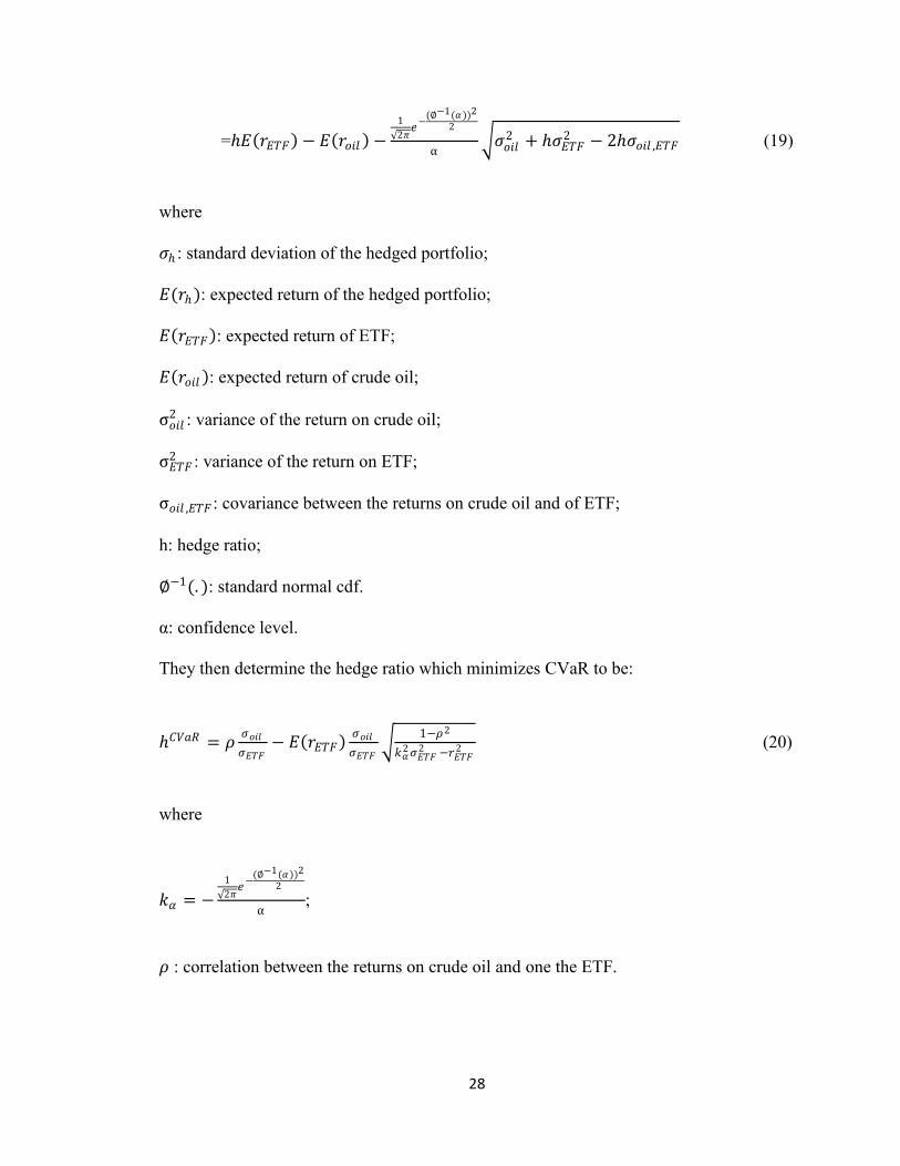
28
=𝐸 𝑟𝐸𝑇𝐹 − 𝐸 𝑟𝑜𝑖𝑙 −
1
2𝜋𝑒
−(∅−1(𝛼))2
2
α 𝜍𝑜𝑖𝑙
2 + 𝜍𝐸𝑇𝐹2 − 2𝜍𝑜𝑖𝑙 ,𝐸𝑇𝐹 (19)
where
𝜍 : standard deviation of the hedged portfolio;
𝐸(𝑟): expected return of the hedged portfolio;
𝐸 𝑟𝐸𝑇𝐹 : expected return of ETF;
𝐸 𝑟𝑜𝑖𝑙 : expected return of crude oil;
σ𝑜𝑖𝑙2 : variance of the return on crude oil;
σ𝐸𝑇𝐹2 : variance of the return on ETF;
σ𝑜𝑖𝑙 ,𝐸𝑇𝐹 : covariance between the returns on crude oil and of ETF;
h: hedge ratio;
∅−1(. ): standard normal cdf.
α: confidence level.
They then determine the hedge ratio which minimizes CVaR to be:
𝐶𝑉𝑎𝑅 = 𝜌𝜍𝑜𝑖𝑙
𝜍𝐸𝑇𝐹− 𝐸 𝑟𝐸𝑇𝐹
𝜍𝑜𝑖𝑙
𝜍𝐸𝑇𝐹
1−𝜌2
𝑘𝛼2𝜍𝐸𝑇𝐹
2 −𝑟𝐸𝑇𝐹2 (20)
where
𝑘𝛼 = −
1
2𝜋𝑒
−(∅−1(𝛼))2
2
α;
𝜌 : correlation between the returns on crude oil and one the ETF.

29
Measure of risk is MVaR
As traditional VaR only considers the first two moments (mean and standard deviation)
of a distribution, the risk estimated by VaR model may be biased if the distribution has a
fat tail. Favre and Galeano (2002) propose a method called Modified Value at Risk
(MVaR) to measure the risk of a portfolio with non-normally distributed returns.
Modified Value at Risk (MVaR) takes into account the skewness and kurtosis of the
return on the portfolio as well as the expected return and standard deviation of return on
the portfolio. Gregoriou and Gueyie (2003) claim that MVaR is a better measure to
investigate extremely negative returns and non-normally distributed returns of portfolios
because MVaR considers skewness and kurtosis of a distribution. Using MVaR as a
measure of risk, the objective function becomes:
Min MVaR = −E 𝑟 + σh zα + 𝑧α
2−1 𝑆𝑖
6+
𝑧α3−3zα 𝐸𝑖
24−
2𝑧α3−5zα 𝑆𝑖
2
36 (21)
with respect to h
where
E(𝑟) = E(𝑟𝑜𝑖𝑙 ) − h𝐸 𝑟𝐸𝑇𝐹
σ2 = σ𝑜𝑖𝑙
2 + 2σ𝐸𝑇𝐹2 − 2hσ𝑜𝑖𝑙 ,𝐸𝑇𝐹
E 𝑟 : expected return of the hedged portfolio;
E(𝑟𝑜𝑖𝑙 ): expected return of crude oil;
zα : αth percentile of the standard normal distribution;
σoil : standard deviation of the return on crude oil;
σETF : standard deviation of the return on the ETF;
σ𝑜𝑖𝑙 ,𝐸𝑇𝐹 : covariance between the returns on crude oil and on the ETF;

30
𝑆𝑖 : skewness of the return on the hedged portfolio;
𝐸𝑖 : kurtosis of the return on the hedged portfolio;
The optimal hedge ratio which minimizes MVaR is given by:
𝑀𝑉𝑎𝑅 = 𝜌𝜍𝑜𝑖𝑙
𝜍𝐸𝑇𝐹− E(r𝐸𝑇𝐹
α )𝜍𝑜𝑖𝑙
𝜍𝐸𝑇𝐹 1−𝜌2
zα+ 𝑧α2−1 ∗𝑆𝑖
6+ 𝑧α3−3zα ∗
𝐸𝑖
24− 2𝑧α
3−5zα ∗𝑆𝑖
2
36
2
𝜍𝐸𝑇𝐹2 −𝑟𝐸𝑇𝐹
2
(22)
where
𝜌 : correlation between the returns on crude oil and on the ETF.
Hedging Effectiveness Measures
Ederington (1979) defines the hedging effectiveness of a futures contract as:
HEvariance = 1 −Variance hedged
Variance unhedged (23)
where
Variancehedged=variance of the change in value of the optimal hedged portfolio;
Varianceunhedged=variance of the change in value of the unhedged portfolio.
This hedging effectiveness measure has been extensively applied in the literature to
evaluate hedging effectiveness (Floros and Vougas, 2008, 1991; Chen and Ford, 2010).
The advantage of Ederington’s measure is that it is simple to apply and interpret. There
are, however, some disadvantages of this measurement. First, since it is based on the
mean-variance approach to portfolio selection, it does not distinguish between upside and
downside risks. Second, it is based on the implicit assumption that the hedged portfolio
return is normally distributed, which may not always be the case.

31
Therefore, I use three other comparable measures to estimate the hedging effectiveness,
the proportionate reduction in the VaR, CVaR and MVaR of the hedged portfolio. The
corresponding hedging effectiveness measures are as follows:
HEVaR =VaR unhedged −VaR hedged
VaR unhedged (24)
where
VaRunhedged : VaR of the return on unhedged crude oil;
VaRhedged : VaR of the return on hedged portfolio obtained by minimizing the VaR.
HECVaR =CVaR unhedged −CVaR hedged
CVaR unhedged (25)
where
CVaRunhedged : CVaR of the return on unhedged crude oil;
CVaRhedged : CVaR of the return on hedged portfolio obtained by minimizing the CVaR.
HEMVaR =MVaR unhedged −MVaR hedged
MVaR unhedged (26)
where
MVaRunhedged : MVaR of the return on unhedged crude oil;
MVaRhedged : MVaR of the return on hedged portfolio obtained by minimizing the MVaR.
I break the dataset into two periods, the in-sample period and the out-of-sample period.
The in-sample period is from the inception date of each ETF to December 31, 2009 and
the out-of-sample period is from January 1, 2010 to January 11, 2012. For the OLS
regression, the daily change in the crude oil prices is regressed on the change in the ETF
price as in Equation (4) to estimate optimal hedge ratios under the MVHR model first by
using in-sample data. The hedge ratios are derived from the slope coefficients in Equation
32
(4) and hedging effectiveness is estimated as the R-square of the regressions. Second, the
estimated hedge ratios are applied to out-of-sample data to calculate the out-of-sample
hedging effectiveness of each ETF (Equation 23). For the GARCH approach, the time-
varying hedge ratio is estimated by using the in-sample data. After obtaining the
estimated parameters of Equation (10) and Equation (11), I calculate the hedge ratio as it
is shown in Equation (12) for each day and then calculate the in-sample hedging
effectiveness. The estimated parameters from the in-sample period are applied to out-of-
sample data to compute the conditional variance and covariance, hedge ratio and out-of-
sample hedging effectiveness.
In applying the hedging models based on VaR, CVaR and MVaR, first, I use the in-
sample data to estimate the optimal hedge ratios which minimize VaR, CVaR and MVaR,
respectively. A confidence level of 95% is selected to reflect portfolio managers’ risk
preference. The optimal hedge ratio for each ETF is then used in equation (14), (18) and
(21) to calculate the VaR, CVaR and MVaR of the hedged portfolio, respectively.
Equations (24), (25) and (26) are applied to calculate hedging effectiveness, respectively
for both periods.
However, the significance of differences in hedging effectiveness among these four
categories of ETFs remains uncertain. Therefore, a t-test is conducted to examine whether
the hedging effectiveness of each category is significantly different from those of the
others. At a significance level of 0.1%, the critical value is 2.326. Therefore, if the t-
statistics is less than 2.326, the null hypothesis of no difference between the hedging
effectiveness of the categories will be rejected.
33
Chapter V. Empirical Results
Results of the MVHR model
Results based on OLS
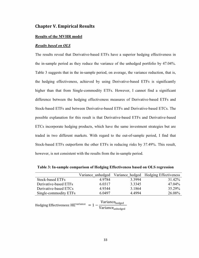
The results reveal that Derivative-based ETFs have a superior hedging effectiveness in
the in-sample period as they reduce the variance of the unhedged portfolio by 47.04%.
Table 3 suggests that in the in-sample period, on average, the variance reduction, that is,
the hedging effectiveness, achieved by using Derivative-based ETFs is significantly
higher than that from Single-commodity ETFs. However, I cannot find a significant
difference between the hedging effectiveness measures of Derivative-based ETFs and
Stock-based ETFs and between Derivative-based ETFs and Derivative-based ETCs. The
possible explanation for this result is that Derivative-based ETFs and Derivative-based
ETCs incorporate hedging products, which have the same investment strategies but are
traded in two different markets. With regard to the out-of-sample period, I find that
Stock-based ETFs outperform the other ETFs in reducing risks by 37.49%. This result,
however, is not consistent with the results from the in-sample period.
Table 3: In-sample comparison of Hedging Effectiveness based on OLS regression
Variance_unhedged Variance_hedged Hedging Effectiveness
Stock-based ETFs 4.9784 3.3994 31.42%
Derivative-based ETFs 6.0317 3.3345 47.04%
Derivative-based ETCs 4.9344 3.1864 35.29%
Single-commodity ETFs 6.0497 4.4994 26.08%
Hedging Effectiveness: HEvariance = 1 −Variancehedged
Varianceunhedged

34
Table 4: Comparison of hedging effectiveness based on the OLS regression for the
different categories of ETFs: in-sample period
OLS
T statistic
Derivative-
based ETFs
Derivative-based
ETCs
Single commodity
ETFs
Stock-based ETFs -1.56 -1.12 1.05
(0.1361) (0.2817) (0.3059)
Derivative-based
ETFs
1.15 2.81***
(0.2654) (0.0086)
Derivative-based
ETCs
1.72*
(0.0984)
***indicates significance at the 99% confidence level;
** indicates significance at the 95% confidence level;
*indicates significance at the 99% confidence level.
Table 5: Out-of-sample comparison of Hedging Effectiveness using OLS regression
Variance_unhedge
d
Variance_hedge
d
Hedging
Effectiveness
Stock-based ETFs 3.0351 1.8974 37.49%
Derivative-based ETFs 3.0451 1.9882 34.74%
Derivative-based ETCs 3.0670 1.9461 36.55%
Single-commodity
ETFs 3.0551 2.3523 23.01%
Hedging Effectiveness: 𝐻𝐸𝑣𝑎𝑟𝑖𝑎𝑛𝑐𝑒 = 1 −𝑉𝑎𝑟𝑖𝑎𝑛𝑐𝑒𝑒𝑑𝑔𝑒𝑑
𝑉𝑎𝑟𝑖𝑎𝑛𝑐𝑒𝑢𝑛𝑒𝑑𝑔𝑒𝑑
35
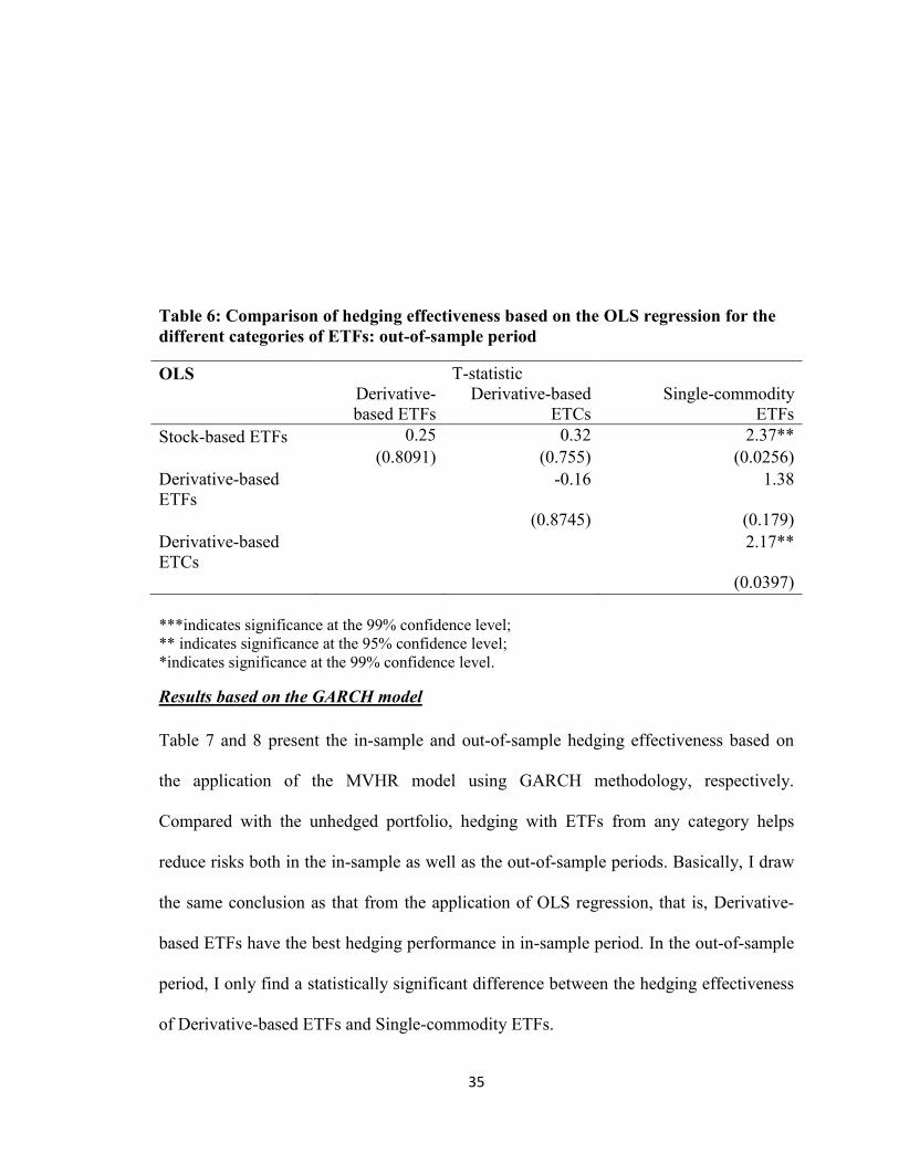
Table 6: Comparison of hedging effectiveness based on the OLS regression for the
different categories of ETFs: out-of-sample period
OLS
T-statistic
Derivative-
based ETFs
Derivative-based
ETCs
Single-commodity
ETFs
Stock-based ETFs 0.25 0.32 2.37**
(0.8091) (0.755) (0.0256)
Derivative-based
ETFs
-0.16 1.38
(0.8745) (0.179)
Derivative-based
ETCs
2.17**
(0.0397)
***indicates significance at the 99% confidence level;
** indicates significance at the 95% confidence level;
*indicates significance at the 99% confidence level.
Results based on the GARCH model
Table 7 and 8 present the in-sample and out-of-sample hedging effectiveness based on
the application of the MVHR model using GARCH methodology, respectively.
Compared with the unhedged portfolio, hedging with ETFs from any category helps
reduce risks both in the in-sample as well as the out-of-sample periods. Basically, I draw
the same conclusion as that from the application of OLS regression, that is, Derivative-
based ETFs have the best hedging performance in in-sample period. In the out-of-sample
period, I only find a statistically significant difference between the hedging effectiveness
of Derivative-based ETFs and Single-commodity ETFs.

36
I examine whether application of the GARCH model is superior to application of OLS
since the GARCH model allows variation in the variances and covariances over time.
Comparing Table 3 with Table 7 and Table 5 with Table 9, I note that the measures of
hedging effectiveness which result from application of the GARCH methodology are
higher than those which result from application of OLS regression. For example, on using
the GARCH model, Derivative-based ETFs lower the variance of the unhedged portfolio
by 55.07% and 56.27% in the in-sample period and the out-of-sample period,
respectively. On applying the OLS regression, 47.04% and 34.74% of the variance of the
unhedged portfolio has been reduced in the in-sample period and out-of-sample period,
respectively. The results indicate that a hedging strategy based on application of the
bivariate GARCH model is superior to hedging based on application of OLS regression.
However, the disadvantage of application of the GARCH methodology is that frequent
rebalancing of the portfolio could result in high transaction costs.
Table 7: In-sample comparison of Hedging Effectiveness based on GARCH
Variance_unhedge
d
Variance_hedge
d
Hedging
Effectiveness
Stock-based ETFs 4.9784 3.3861 31.66%
Derivative-based ETFs 6.0317 2.8101 55.07%
Derivative-based ETCs 4.9344 3.1137 36.86%
Single-commodity
ETFs 6.0497 4.1789 30.87%
Hedging Effectiveness: HEvariance = 1 −Variancehedged
Varianceunhedged

37
Table 8: Comparison of hedging effectiveness based on the GARCH model for the
different categories of ETFs: in-sample period
GARCH
T-statistic
Derivative-
based ETFs
Derivative-based
ETCs
Single-commodity
ETFs
Stock-based ETFs -2.47** -2.45** 0.15
(0.0232) (0.0281) (0.885)
Derivative-based
ETFs
1.91* 3.31***
(0.071) (0.0025)
Derivative-based
ETCs
1.1
(0.2831)
***indicates significance at the 99% confidence level;
** indicates significance at the 95% confidence level;
*indicates significance at the 99% confidence level.
Table 9: Out-of-sample comparison of Hedging Effectiveness based on GARCH
Variance_unhedge
d
Variance_hedge
d
Hedging
Effectiveness
Stock-based ETFs 3.0351 1.8531 38.94%
Derivative-based ETFs 3.0437 1.3320 56.27%
Derivative-based ETCs 3.0670 1.9101 37.73%
Single-commodity
ETFs 3.0551 2.0690 32.29%
Variance Reduction: HEvariance = 1 −Variancehedged
Varianceunhedged

38
Table 10: Comparison of hedging effectiveness based on the MVHR model for the
different categories of ETFs: out-of-sample period
GARCH
T-statistic
Derivative-
based ETFs
Derivative-based
ETCs
Single commodity based
ETFs
Stock-based ETFs -1.34 0.49 0.9
(0.1947) (0.6345) (0.3758)
Derivative-based
ETFs
1.44 2.41**
(0.1661) (0.0222)
Derivative-based
ETCs
0.74
(0.4669)
***indicates significance at the 99% confidence level;
** indicates significance at the 95% confidence level;
*indicates significance at the 99% confidence level.
Results based on minimizing VaR
Table 11: In-sample comparison of Hedging Effectiveness based on VaR
VaR_unhedged VaR_hedged Hedging Effectiveness
Stock-based ETFs 0.0611 0.0511 16.31%
Derivative-based ETFs 0.0716 0.0475 33.55%
Derivative-based ETCs 0.0603 0.0511 15.24%
Single commodity ETFs 0.0691 0.0587 15.13%
Hedging Effectiveness: HEVaR =VaRunhedged − VaRhedged
VaRunhedged
From Table 11, I note that in the in-sample period, hedging based on minimizing VaR is
effective in reducing the VaR of the portfolio consisting of crude oil and energy ETFs for
all four categories of ETFs. Derivative-based ETFs outperforms the other three groups
with an in-sample hedging effectiveness of 33.55%, while Stock-based ETFs, Derivative-
based ETCs and Single-commodity ETFs just have a hedging effectiveness of around
15%. Stock-based ETFs rank second in hedging effectiveness as this group has an in-
39
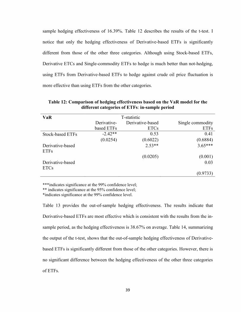
sample hedging effectiveness of 16.39%. Table 12 describes the results of the t-test. I
notice that only the hedging effectiveness of Derivative-based ETFs is significantly
different from those of the other three categories. Although using Stock-based ETFs,
Derivative ETCs and Single-commodity ETFs to hedge is much better than not-hedging,
using ETFs from Derivative-based ETFs to hedge against crude oil price fluctuation is
more effective than using ETFs from the other categories.
Table 12: Comparison of hedging effectiveness based on the VaR model for the
different categories of ETFs: in-sample period
VaR
T-statistic
Derivative-
based ETFs
Derivative-based
ETCs
Single commodity
ETFs
Stock-based ETFs -2.42** 0.53 0.41
(0.0254) (0.6022) (0.6884)
Derivative-based
ETFs
2.53** 3.65***
(0.0205) (0.001)
Derivative-based
ETCs
0.03
(0.9733)
***indicates significance at the 99% confidence level;
** indicates significance at the 95% confidence level;
*indicates significance at the 99% confidence level.
Table 13 provides the out-of-sample hedging effectiveness. The results indicate that
Derivative-based ETFs are most effective which is consistent with the results from the in-
sample period, as the hedging effectiveness is 38.67% on average. Table 14, summarizing
the output of the t-test, shows that the out-of-sample hedging effectiveness of Derivative-
based ETFs is significantly different from those of the other categories. However, there is
no significant difference between the hedging effectiveness of the other three categories
of ETFs.

40
Table 13: Out-of-sample comparison of Hedging Effectiveness based on VaR
VaR_unhedged VaR_hedged Hedging Effectiveness
Stock-based ETFs 0.0383 0.0300 21.50%
Derivative-based ETFs 0.0383 0.0235 38.67%
Derivative-based ETCs 0.0383 0.0304 20.63%
Single commodity based ETFs 0.0383 0.0310 18.99%
Hedging Effectiveness: HEVaR =VaR unhedged −VaR hedged
VaR unhedged
Table 14: Comparison of hedging effectiveness based on the VaR model for the
different categories of ETFs: out-of-sample period
VaR
T-statistic
Derivative-based
ETFs
Derivative-based
ETCs
Single commodity
ETFs
Stock-based ETFs -1.69 0.38 0.55
(0.1074) (0.7075) (0.589)
Derivative-based
ETFs
1.76* 2.67**
(0.0952) (0.0122)
Derivative-based
ETCs
0.34
(0.7338)
***indicates significance at the 99% confidence level;
** indicates significance at the 95% confidence level;
*indicates significance at the 99% confidence level.
Results based on minimizing CVaR
From Table 15, we note that the hedging based on CVaR is effective in reducing the
CVaR of the portfolio incorporating crude oil and energy ETFs for all four categories.
Derivative-based ETFs outperform the other three groups with a hedging effectiveness of
29.45% while hedging using Stock-based ETFs, Derivative ETCs and Single-commodity
ETFs just has a hedging effectiveness around 16%. Derivative-based ETCs are ranked
second in hedging effectiveness as they reduce the VaR of the portfolio by 17.18%. From

41
Table 16, which presents the results of the t-test, I note that only the hedging
effectiveness of Stock-based ETFs is significantly different from that of ETFs in the other
three categories. Thus, using Derivative-based ETFs to hedge against crude oil price
fluctuation is more effective than using ETFs from the remaining categories and the
hedging performance of Stock-based ETFs, Derivative-based ETCs and Single-
commodity ETFs are almost the same. Admittedly, using Stock-based ETFs, Derivative-
based ETCs and Single-commodity ETFs to hedge is much better than not-hedging as the
VaR of the hedged portfolio has been decreased by 16% on average.
Table 15: In-sample comparison of Hedging Effectiveness based on CVaR
CVaR_unhedged CVaR_hedged Hedging Effectiveness
Stock-based ETFs 0.0821 0.0682 16.96%
Derivative-based ETFs 0.0907 0.0639 29.45%
Derivative-based ETCs 0.0816 0.0677 17.18%
Single commodity ETFs 0.0880 0.0744 15.54%
Hedging Effectiveness: HECVaR =CVaR unhedged −CVaR hedged
CVaR unhedged
Table 16: Comparison of hedging effectiveness based on the CVaR model for the
different categories of ETFs: in-sample period
CVaR
T-statistic
Derivative-
based ETFs
Derivative-based
ETCs
Single commodity
ETFs
Stock-based ETFs -2.02* -0.05 0.5
(0.0572) (0.963) (0.6231)
Derivative-based
ETFs
1.73* 3.1**
(0.0991) (0.0042)
Derivative-based
ETCs
0.41
(0.6868)
***indicates significance at 0.01 level;
** indicates significance at 0.05 level;
*indicates significance at 0.1 level.
42
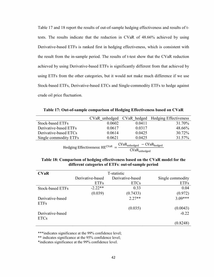
Table 17 and 18 report the results of out-of-sample hedging effectiveness and results of t-
tests. The results indicate that the reduction in CVaR of 48.66% achieved by using
Derivative-based ETFs is ranked first in hedging effectiveness, which is consistent with
the result from the in-sample period. The results of t-test show that the CVaR reduction
achieved by using Derivative-based ETFs is significantly different from that achieved by
using ETFs from the other categories, but it would not make much difference if we use
Stock-based ETFs, Derivative-based ETCs and Single-commodity ETFs to hedge against
crude oil price fluctuation.
Table 17: Out-of-sample comparison of Hedging Effectiveness based on CVaR
CVaR_unhedged CVaR_hedged Hedging Effectiveness
Stock-based ETFs 0.0602 0.0411 31.70%
Derivative-based ETFs 0.0617 0.0317 48.66%
Derivative-based ETCs 0.0614 0.0425 30.72%
Single commodity ETFs 0.0621 0.0425 31.57%
Hedging Effectiveness: HECVaR =CVaRunhedged − CVaRhedged
CVaRunhedged
Table 18: Comparison of hedging effectiveness based on the CVaR model for the
different categories of ETFs: out-of-sample period
CVaR
T-statistic
Derivative-based
ETFs
Derivative-based
ETCs
Single commodity
ETFs
Stock-based ETFs -2.22** 0.33 0.04
(0.039) (0.7433) (0.972)
Derivative-based
ETFs
2.27** 3.09***
(0.035) (0.0043)
Derivative-based
ETCs
-0.22
(0.8248)
***indicates significance at the 99% confidence level;
** indicates significance at the 95% confidence level;
*indicates significance at the 99% confidence level.

43
Results based on minimizing MVaR
From Table 19, we can see that hedging based on MVaR is effective in reducing the
MVaR of the portfolio of crude oil and energy ETFs for all four categories in the in-
sample period. Stock-based ETFs outperform ETFs from the other three categories with a
hedging effectiveness of 47.54%, while hedging by using Stock-based ETFs, Derivative-
based ETCs and Single-commodity ETFs just has a hedging effectiveness of around 16%.
From Table 20, I note that only the hedging effectiveness of Derivative-based ETFs is
significantly different from those of the other three categories of ETFs, which means that
using Derivative-based ETFs to hedge against crude oil price fluctuation is more effective
than using other ETFs from the rest categories; on the other hand, the hedging
performance of Stock-based ETFs, Derivative-based ETCs and Single-commodity ETFs
is almost the same.
Table 19: In-sample comparison of Hedging Effectiveness based on MVaR
MVaR_unhedged MVaR_hedged Hedging Effectiveness
Stock-based ETFs 0.0621 0.0496 20.06%
Derivative-based ETFs 0.0688 0.0324 47.54%
Derivative-based ETCs 0.0648 0.0547 15.63%
Single commodity ETFs 0.0702 0.0584 16.78%
Hedging Effectiveness: HEMVaR =MVaRunhedged − MVaRhedged
MVaRunhedged

44
Table 20: Comparison of hedging effectiveness based on the MVaR model for the
different categories of ETFs: in-sample period
MVaR
T-statistic
Derivative-based
ETFs
Derivative-based
ETCs
Single commodity
ETFs
Stock-based ETFs -2.4** 1.46 1
(0.0268) (0.1663) (0.326)
Derivative-based
ETFs
2.74** 3.99***
(0.013) (0.0004)
Derivative-based
ETCs
-0.31
(0.7592)
***indicates significance at the 99% confidence level;
** indicates significance at the 95% confidence level;
*indicates significance at the 99% confidence level.
Table 21 and 22 show the results of out-of-sample hedging effectiveness and the results
of the t-tests. As Table 20 indicates, the reduction in MVaR is more effective when using
Derivative-based ETFs with reduction of MVaR of the hedged portfolio by 31.79%,
which is consistent with the result from the in-sample period. The results of the t-tests
show that the hedging effectiveness of Derivative-based ETFs is significantly different
from those of the other categories, but it would not make much difference if we use
Stock-based ETFs, Derivative-based ETCs and Single-commodity ETFs to hedge against
crude oil price fluctuation.
Table 21: Out-of-sample comparison of Hedging Effectiveness based on MVaR
MVaR_unhedged MVaR_hedged Hedging Effectiveness
Stock-based ETFs 419 0.0327 21.98%
Derivative-based ETFs 0.0420 0.0239 43.00%
Derivative-based ETCs 0.0420 0.0314 25.39%
Single commodity ETFs 0.0419 0.0323 22.94%
Hedging Effectiveness: HEMVaR =MVaR unhedged −MVaR hedged
MVaR unhedged

45
Table 22: Comparison of hedging effectiveness based on the MVaR model for the
different categories of ETFs: out-of-sample period
MVaR
T-statistic
Derivative-based
ETFs
Derivative-based
ETCs
Single commodity
ETFs
Stock-based ETFs -2.11 -0.79 -0.22
(0.0481) (0.4432) (0.8312)
Derivative-based
ETFs
1.68 2.77
(0.1095) (0.0095)
Derivative-based
ETCs
0.47
(0.6438)
***indicates significance at the 99% confidence level;
** indicates significance at the 95% confidence level;
*indicates significance at the 99% confidence level.
Chapter VI. Conclusion and Discussion
This thesis investigates the hedging effectiveness of energy ETFs. I use 48 energy ETFs
listed in US, Canada and London markets to examine whether they are effective in
reducing the risk of crude oil price fluctuation. I categorize these ETFs into four
categories based on their investment strategy and their top holdings (Table 1). I study the
performance of the ETFs in the overall period starting from the inception date of each
ETF till January 11, 2012. The overall period is split into the in-sample period and the
out-of-sample period. The in-sample period covers the period from the inception date of
each ETF till December 31, 2010 and is used to estimate optimal hedge ratios and in-
sample hedging effectiveness. The out-of-sample period covers the period from January 1,
2011 till January 11, 2012 and is used to apply the optimal hedge ratios and calculate out-
of-sample hedging effectiveness. The hedge ratios and measures of hedging effectiveness
46
are based on: 1) the minimum variance hedge ratio (MVHR) model, which is applied by
using two methods to estimate the optimal hedge ratios, an OLS regression and GARCH
methodology; 2) models based on minimizing measures of risk based on value at risk
(VaR), which are in turn, VaR, CVaR and MVaR.
The in-sample hedging effectiveness measures estimated by the five methods indicate
that Derivative-based ETFs, which are traded in the US market and invest in derivatives
such as futures and swaps, have the best hedging performance while there are no
significant differences between the hedging performance of Stock-based ETFs,
Derivative-based ETCs and Single-commodity ETFs. The poor performance of these
ETFs could be due to several reasons. First, futures contracts are an effective way to
hedge against oil price fluctuation but futures contracts are not accessible to small
investors. Derivative-based ETFs may have some features of futures contracts since their
asset allocation contains futures. The reason that Derivative-based ETFs outperform
Derivative-based ETCs is probably due to differences in the regulation between the U.S.
and U.K. markets. Since Stock-based ETFs just invest in the stocks of energy
corporations, the price of these ETFs may not just be affected by crude oil prices but by
other factors such as the company’s own performance, which could affect the hedging
effectiveness.
In the out-of-sample period, results from application of the VaR, CVaR and MVaR as
measures of risk are consistent with those from the in-sample period. Hedging by
Derivative-based ETFs is the most effective hedging instrument. Compared with the
conventional hedging method OLS, hedging using a GARCH model, which takes into
47
account time-varying variance, helps to reduce more risks. However, the downside of the
bivariate GARCH model is the higher transaction cost caused by frequent rebalancing of
the hedged portfolio.
In summary, energy ETFs, especially ones with investment in futures contracts, provide
an effective way for small investors to hedge against crude oil price fluctuation. While,
this thesis is limited to using energy ETFs to hedge against crude oil price fluctuation, in
future research, the examination of hedging effectiveness can be extended to ETFs from
other sectors such as real estate to hedge against the corresponding commodity price
fluctuation. Also the hedging effectiveness of ETFs listed in different markets can be
examined. Another extension could combine time-varying variances and covariances
with the VaR or CVaR approach as recommended by Cao, Harris and Shen (2008).

48
References
Aber, J. W., Li, D., and Can, L. (2009), Price Volatility and Tracking Ability of ETFs. Journal of Asset
Management, 10, 4: 210-221.
Ackermann, C., R. McEnally, and Ravenscraft, D. (1999), The Performance of Hedge Funds: Risk, Return,
and Incentives. Journal of Finance, 54, 3: 833–874.
Alexander, G., Baptista, A. (2006), Does the Basle Capital Accord Reduce Bank Fragility? An Assessment
of the Value-at-Risk Approach. Journal of Monetary Economics, 53, 7: 1631-1660.
Baillie, R. T., Myers, R. J. (1991), Bivariate GARCH Estimation of the Optimal Commodity Futures Hedge.
Journal of Applied Econometrics, 6, 2: 109–124.
Bawa, V.S. (1975), Optimal Rules for Ordering Uncertain Prospects, Journal of Financial Economics, 2, 1:
95-121.
Bienkowski, Nik. (2007), Exchange Traded Commodities Led by Gold: ETFs Opened the World of
Commodities to Investors. The London Bullion Market Association, 48: 6-8.
Bollerslev, T. (1996), Generalized Autoregressive Conditional Heteroskedasticity, Journal of Econometrics,
31, 3: 307-327.
Brooks, C., Chong, J. (2001), The Cross-currency Hedging Performance of Implied Versus Statistical
Forecasting Models. Journal of Futures Markets, 21, 11: 1043-1069.
Brooks, C., (2008), Introductory Econometrics for Finance. Cambridge University Press, Second Edition,
432-444.
Brooks, C., Henry, O. T., Persand, G. (2002), The effects of Asymmetries on Optimal Hedge Ratios.
Journal of Business, 75, 2: 333-352.
49
Cao, Z., Harris, R. and Shen, J., (2010), Hedging and Value at Risk: A Semi-Parametric Approach. Journal
of Futures Markets, 30, 8: 780-799.
Chi, G.T., Zhao, G.J., Yang, Z.Y., (2009), Futures Optimal Hedge Ratio Model Based on CVaR and Its
Application. Journal of Systems & Management, 18, 1: 27-33.
Dowd, K. (2000), Adjusting for Risk: An Improved Sharpe Ratio. International Review of Economics &
Finance, 9, 3: 209–222.
Duffie, D., and Pan, J., (1997), An overview of value at risk, Journal of Derivatives, 4, 3: 7-49.
Ederington, L. H. (1979), The Hedging Performance of the New Futures Markets. Journal of Finance, 34, 1:
157–170.
Eling, M. (2008), Does the Measure Matter in the Mutual Fund Industry? Financial Analysts Journal, 64, 3:
54-66.
Favre, L., Galeano, J. (2002), Mean-modified Value-at-Risk Optimization with Hedge Funds. Journal of
Alternative investments, 5, 2: 21-31.
Floros, C., Vougas, D. V. (2008), Hedging Effectiveness in Greek Stock Index Futures Market, working
paper.
Gregoriou, G.N., and J.P. Gueyie (2003), Risk-Adjusted Performance of Funds of Hedge Funds Using a
Modified Sharpe Ratio. Journal of wealth Management, 6, 3: 77–83.
Hull, J. C., and White, A. (1998), Value-at-Risk When Daily Changes in Market Variables are not
Normally Distributed, Journal of Derivatives, 5, 3 : 9-19.
Jackson, P., Maude, D. J. and Perraudin, W. (1997), Bank Capital and Value at Risk. Journal of Derivatives,
4: 73-89.
50
Johnson, L. L. (1960), The Theory of Hedging and Speculation in Commodity Futures. Review of
Economic Studies, 27, 3: 139–151.
Jorion, P. (2000), Value at Risk: the New Benchmark for Controlling Market Risk. Irvin Professional Pub.
Junkus, J. C. and Lee, C. F. (1985), Use of Three Index Futures in Hedging Decisions. Journal of Futures
Markets, 5, 2: 201–222.
Kosev, M., Williams, T. (2011), Exchange Traded Funds. Reserve Bank of Australia Bulletin, March
Quarter: 51-60.
Kostovetsky, L. (2003). Index Mutual Funds and Exchange-traded Funds: A Comparison of two Methods
of Passive investment. The Journal of Portfolio Management, 29, 4: 80-94.
Lien, D., & Tse, Y. K. (1998), Hedging Time-varying Downside Risk. Journal of Futures Markets, 18, 6:
705–722.
Lien, D., & Tse, Y. K. (2000), Hedging Downside Risk with Futures Contracts. Applied Financial
Economics, 10, 2: 163–170.
Myers, R. J., and Thompson, S. R. (1989), Generalized Optimal Hedge Ratio Estimation. American Journal
of Agricultural Economics, 71, 4: 858–868.
Park, T. H., Switzer, L. (1995), Time-varying Distribution and the Optimal Hedge Ratios for Stock Index
Futures. Applied Financial Economics, 15, 1: 131-137.
Pflug, G. Ch. (2000), Some Remarks on the Value-at-risk and the Conditional Value-at-Risk. Probabilitic
Constrained Optimization: Methodology and Applications.
Redefining the Commodities Marketplace, Exchange Traded Commodities. (2009), London Stock
Exchange.
51
Rockafellar, R. T., Uryasev, S. (2000), Optimization of Conditional Value-at-risk. Journal of Risk, 2, 3: 21-
41.
Rompotis, G. G. (2009a). Interfamily Competition on Index Tracking: The Case of the Vanguard ETFs and
Index Funds. Journal of Asset Management, 10, 4: 263- 278.