Hector user manual version 1 - Welcome to SEGALsegal.ubi.pt/hector/manual_1.6.pdf · Hector is...

Hector user manual

version 1.6

Machiel Bos and Rui Fernandes

October 19, 2016

Contents

1 Introduction 2

1.1 How to cite Hector . . . . . . . . . . . . . . . . . . . . . . . . . . . . 31.2 Main features . . . . . . . . . . . . . . . . . . . . . . . . . . . . . . . 3

2 Installation 4

3 Hector conventions 4

4 Tutorial 5

4.1 Example 1: Synthetic GPS time series with spikes and offsets . . . . . . 54.1.1 Removal of outliers . . . . . . . . . . . . . . . . . . . . . . . . 64.1.2 Estimation of the linear trend . . . . . . . . . . . . . . . . . . . 74.1.3 Plotting the power spectral density . . . . . . . . . . . . . . . . 12

4.2 Example 2: The monthly PSMSL tide gauge data at Cascais . . . . . . 144.3 Example 3: Creating synthetic coloured noise . . . . . . . . . . . . . . 154.4 Example 4: Estimating amplitude of post-seismic relaxation . . . . . . . 174.5 Example 5: Including extra geophysical signals for multivariate analysis 174.6 Example 6: Estimating multilinear trends . . . . . . . . . . . . . . . . . 17

5 Model specification 18

5.1 Post-seismic deformation . . . . . . . . . . . . . . . . . . . . . . . . . 185.2 Multi-trend . . . . . . . . . . . . . . . . . . . . . . . . . . . . . . . . . 19

6 Acceptable data format 19

6.1 mom-format . . . . . . . . . . . . . . . . . . . . . . . . . . . . . . . . 206.2 enu-format . . . . . . . . . . . . . . . . . . . . . . . . . . . . . . . . . 206.3 neu-format . . . . . . . . . . . . . . . . . . . . . . . . . . . . . . . . . 206.4 rlrdata-format . . . . . . . . . . . . . . . . . . . . . . . . . . . . . . . 20

7 Implemented Noise Models 20

7.1 White noise . . . . . . . . . . . . . . . . . . . . . . . . . . . . . . . . 217.2 Power-law noise . . . . . . . . . . . . . . . . . . . . . . . . . . . . . . 217.3 Power-law approximated . . . . . . . . . . . . . . . . . . . . . . . . . . 21

1

Hector user manual Section 1

7.4 ARFIMA and ARMA . . . . . . . . . . . . . . . . . . . . . . . . . . . 227.5 Generalized Gauss Markov noise model . . . . . . . . . . . . . . . . . . 227.6 Flicker noise and Random Walk noise . . . . . . . . . . . . . . . . . . 23

8 The Akaike and Baysian Information Criteria 23

9 Quick reference for the control-files 24

9.1 removeoutliers.ctl . . . . . . . . . . . . . . . . . . . . . . . . . . . . . 249.2 estimatetrend.ctl . . . . . . . . . . . . . . . . . . . . . . . . . . . . . . 249.3 estimatespectrum.ctl . . . . . . . . . . . . . . . . . . . . . . . . . . . 259.4 modelspectrum.ctl . . . . . . . . . . . . . . . . . . . . . . . . . . . . . 269.5 simulatenoise.ctl . . . . . . . . . . . . . . . . . . . . . . . . . . . . . . 26

10 Advanced Features 27

10.1 Offsets . . . . . . . . . . . . . . . . . . . . . . . . . . . . . . . . . . . 27

11 License and Copyright 27

A History of changes made in the various versions of Hector 29

A.1 Version 1.1 . . . . . . . . . . . . . . . . . . . . . . . . . . . . . . . . . 29A.2 Version 1.2 . . . . . . . . . . . . . . . . . . . . . . . . . . . . . . . . . 29A.3 Version 1.3 . . . . . . . . . . . . . . . . . . . . . . . . . . . . . . . . . 30A.4 Version 1.4 . . . . . . . . . . . . . . . . . . . . . . . . . . . . . . . . . 30A.5 Version 1.5 . . . . . . . . . . . . . . . . . . . . . . . . . . . . . . . . . 30A.6 Version 1.5.1 . . . . . . . . . . . . . . . . . . . . . . . . . . . . . . . . 31A.7 Version 1.5.2 . . . . . . . . . . . . . . . . . . . . . . . . . . . . . . . . 31A.8 Version 1.6 . . . . . . . . . . . . . . . . . . . . . . . . . . . . . . . . . 31

1 Introduction

Hector is a software package that can be used to estimate a trend in time series withtemporal corelated noise. Trend estimation is a common task in geophysical researchwhere one is interested in phenomena such as the increase in temperature, sea level orGNSS derived station position over time. The trend can be linear or a higher degreepolynomial and in addition one can estimate periodic signals, offsets and post-seismicdeformation. Together they represent the model that is fitted to the observations.

It is well known that in most geophysical time series the noise is correlated in time(Agnew, 1992; Beran, 1992) and this has a significant influence on the accuracy by whichthe model parameters can be estimated. Therefore, the use of a computer program suchas Hector is advisable.

Hector assumes that the user knows what type of temporal correlated noise existsin the observations and estimates both the model parameters and the parameters of thechosen noise model using the Maximum Likelihood Estimation (MLE) method. Since formost observations the choice of noise model can be found from literature or by lookingat the power spectral density, this is sufficient in most cases.

of 31


Instead of using Hector, one can also use the CATS software of Williams (2008). Infact, Hector was written from scratch in C++ with the objective to have a faster CATS.The reason is Hector is faster is that it accepts only stationary noise, with constant noiseproperties, and this allows the use of fast matrices operations.

Another alternative is the program est_noise of Langbein (2010). Recent versionsinclude the approach of Bos et al. (2013) to deal with missing data but with a differentway to construct the covariance matrix.

This manual starts in section 2 by explaining how to install Hector on your computerand in section 3 a general description of Hector is given. In section 4 a tutorial on usingHector is presented using two examples of analysing synthetic GPS data with offsets andoutliers and a real GPS data set. This is followed by section 5 where the models thatcan be fitted to the observations are described. Sections 6 and 7 explain the acceptabledata formats and implemented noise models respectively. Finally, a quick reference ofthe parameters in the control-files are presented in 9.

1.1 How to cite Hector

If you find the Hector program useful, please cite it in your work as:

Bos, M. S., Fernandes, R. M. S., Williams, S. D. P., and Bastos, L. (2013).Fast Error Analysis of Continuous GNSS Observations with Missing Data.J.

Geod., Vol. 87(4), 351–360, doi:10.1007/s00190-012-0605-0.

1.2 Main features

The main features of Hector are:

1. Correctly deals with missing data. No interpolation or zero padding of the datanor an approximation of the covariance matrix is required (as long the noise is, orhas been made, stationary).

2. Allows yearly, half-yearly and other periodic signals to be included in the estimationprocess of the linear trend.

3. Allows the option to estimate offsets at given time epochs.

4. Allows to estimate multiple linear trends.

5. Allows to estimate a higher polynomial trend.

6. Allows to estimate post-seismic relaxation using an exponential or logarithmicmodel for given relaxation times.

7. Includes power-law noise, ARFIMA, generalized Gauss-Markov and white noisemodels. Any combination of these models can be made.

8. Comes with programs to remove outliers, to make power spectral density plots andto create files with synthetic coloured noise.

of 31


Table 1: List of programs provided by the Hector software package.Name Description

estimatetrend Main program to estimate a linear trend.estimatespectrum Program to estimate the power spectral density from the

data or residuals using the Welch periodogram method.modelspectrum Given a noise model and values of the noise parame-

ters, this program computed the associated power spec-tral density for given frequency range.

removeoutliers Program to find offsets and to remove outliers from thedata.

simulatenoise Program to files with synthetic coloured noise.date2mjd Small program to convert calender date into Modified

Julian Date.mjd2date The inverse of date2mjd.

2 Installation

The Hector software package is intended to be run on computers with Unix-like operatingsystems. For the previous versions of Hector special debian binary packages were createdbut these were, as far as we know, never used. Also the compilation of the source codewas troublesome for most users because the library names keep on changing and theyare slightly different on the various Linux distributions. For that reason, for the currentversion we only provide the static binaries.

The static binaries (32 & 64 bit) can be obtained from the website: http://segal.ubi.pt/hector.It is advisable to put the binaries in the directory /usr/local/bin. If the binaries are putin another directory, then make sure it’s added to the PATH variable in your shell envi-ronment. The list of programs provides is given in Table 1.

To run the examples that are described in this manual, and which can be downloadedfrom the website, one also need the Tcl scripting language and the gnuplot plottingprogram. Unfortunately, Tcl is largely unknown by the geodetic community and withthe future in mind, some ruby scripts/programs have been added to the distribution.On an Ubuntu machine one can these programs by typing:

sudo apt-get install pgplot tcl ruby-full

3 Hector conventions

Hector consists out of a set of simple programs that help you through the steps of timeseries analysis: removal of outliers, estimation of a trend, estimating the power spectraldensity and modelling of the estimated power spectral density. In addition, programsexist to find offsets in the data and synthetic time series with coloured noise can becreated.

Each program comes with its own control-file where parameter values needed bythe program are given. For example, the program removeoutliers has a control-file

of 31


called removeoutlier.ctl. All programs follow the same naming scheme for theircontrol-files.

This control-file is a simple ASCII text file containing on each row a keyword followedby its value or a list of values. Some keywords are optional and if they are not specified,then the default value will be used. A list of all possible keywords for each control-file isgiven in section 9.

Following the nomenclature of Bevis and Brown (2014), Hector estimates stationtrajectory models. These models can include a trend, seasonal signals, offsets and post-seismic deformation. See section 5 for more details. In Hector you can specify the typeof trend, which seasonal and other periodic signals in the control-file. In addition youcan specify in the control-file if you want to estimate offsets, breaks and/or post-seismicdeformation. These are a kind of global model parameters that you normally apply toall your time series. On the other hand, the time of an offset, break or post-seismicdeformation differs from station to station and are a kind of local model parameters. InHector this information is normally written in the header of the time series.

4 Tutorial

The source code and examples are provides in a separate tar-ball which you can downloadfrom the Hector website and put in any directory you like.

By going step by step through the analysis of some example data sets the workingof Hector will be explained. First, we look at some synthetic GPS data.

4.1 Example 1: Synthetic GPS time series with spikes and offsets

In the directory ex1 a data file called TEST.enu is stored which represents some fic-tional GPS position data set. The file extension ‘enu’ stands for East-North-Up andthese three components are stored in the 2nd, 3rd and 4th column respectively. Thefirst column contains the Modified Julian Date (MJD) which is convenient format tomake plots. You can use the programs date2mjd and date2mjd to convert betweenyear/month/day/hour/minute/second and MJD values. These data are stored in a sim-ple ASCII text file and can be inspected by any normal text editor. When doing so, onewill detect some additional header lines:

# sampling period 1.0

# offset 50284.0 0

# offset 50334.0 0

# offset 50334.0 1

# offset 50784.0 0

# offset 51034.0 0

The first line just tells the program that the sampling period of the data is daily (T=1day). Furthermore, there are offsets at the MJD epochs 50284, 50334, 50784 and 51034.The last 0 indicates that these only occur in the East component (0=East, 1=North,2=Up). If an offset occurs in more than one component, the header line for the offsetis repeated such as is the case for MJD=50334. Hector cannot find the time of offset,these have to be provided by the user.

of 31


-60

-40

-20

0

20

40

60

80

100

120

140

1996 1996.5 1997 1997.5 1998 1998.5 1999

’TEST.enu’ using (($1-51544)/365.25+2000):2

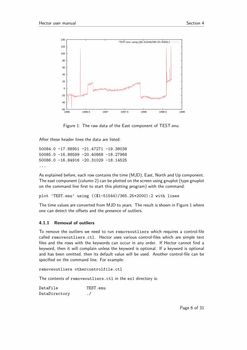
Figure 1: The raw data of the East component of TEST.enu.

After these header lines the data are listed:

50084.0 -17.88951 -21.47271 -19.38038

50085.0 -16.88599 -20.40868 -18.27968

50086.0 -16.84916 -20.31029 -18.14525

...

As explained before, each row contains the time (MJD), East, North and Up component.The east component (column 2) can be plotted on the screen using gnuplot (type gnuploton the command line first to start this plotting program) with the command:

plot ’TEST.enu’ using (($1-51544)/365.25+2000):2 with lines

The time values are converted from MJD to years. The result is shown in Figure 1 whereone can detect the offsets and the presence of outliers.

4.1.1 Removal of outliers

To remove the outliers we need to run removeoutliers which requires a control-filecalled removeoutliers.ctl. Hector uses various control-files which are simple textfiles and the rows with the keywords can occur in any order. If Hector cannot find akeyword, then it will complain unless the keyword is optional. If a keyword is optionaland has been omitted, then its default value will be used. Another control-file can bespecified on the command line. For example:

removeoutliers othercontrolfile.ctl

The contents of removeoutliers.ctl in the ex1 directory is:

DataFile TEST.enu

DataDirectory ./

of 31


OutputFile TEST_pre.mom

component East

interpolate no

seasonalsignal yes

halfseasonalsignal no

estimateoffsets yes

IQ_factor 3.0

PhysicalUnit mm

ScaleFactor 1.0

The first line gives the name of the DataFile with the raw data which is TEST.enuin our case. The second line gives the directory where this file can be found and thethird live contains the required name of the file with the preprocessed data (outliersremoved): TEST_pre.mom. The output will always be in mom-format which stands forMJD, Observations, Model. The last column is optional and since removeoutliers

only replaces the raw observations with the preprocessed observations, no third columnwill be added. See section 6 for more details on the acceptable data format.

removeoutliers fits a linear trend to the raw data using ordinary least-squares andafterwards subtracts this linear trend from the observations to create residuals. Theseresiduals are ordered by size and the interquartile range is computed (this is the valueof the residual at 75% of the sorted array minus the value of the residual at 25% of thesorted array). Any residual with a value less than 3 times this interquartile range belowor above the median is considered to be an outlier (Langbein and Bock, 2004). Thisfactor of 3 is set by the keyword IQ_factor and can be changed by the user.

In this control-file one must also give the physical unit of the data. This informationis not essential but reminds the user to think about the unit of the data and if somescaling is required. Such scaling is set by the keyword ’ScaleFactor’ which is 1.0 in thiscase. This keyword is optional and if omitted then a default value of 1.0 will be assumed.

The linear trend is estimated assuming a white noise model and, as can be seenfrom the removeoutliers.ctl file, a seasonal (i.e. yearly) signal is also included inthe estimation process. Offsets are also estimated. On the other hand, no half-seasonalsignal is estimated nor any other periodic signal and the missing data are not interpolated.The keyword ’periodicsignals’ is optional and can be omitted.

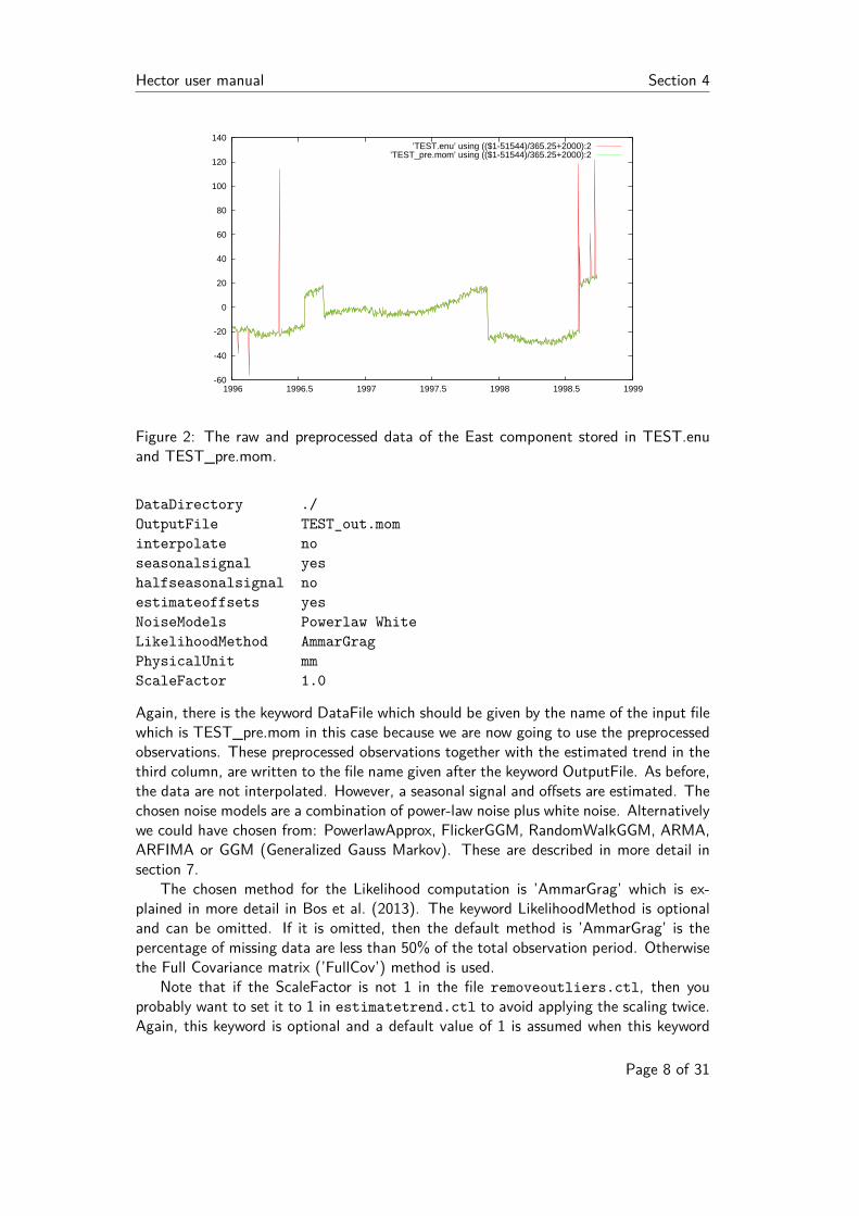
The results of removeoutliers, stored in TEST_pre.mom, are shown in Figure 2which have been generated with gnuplot using the command:

plot ’TEST.enu’ using (($1-51544)/365.25+2000):2 with lines,\

’TEST_pre.mom’ using (($1-51544)/365.25+2000):2 with lines

4.1.2 Estimation of the linear trend

Now that the outliers have been removed, we can estimate the linear trend. The pa-rameters that control this analysis are by default given in the file estimatetrend.ctl.As before, another name for the control-file can be specified on the command line. Thecontents of estimatetrend.ctl is:

DataFile TEST_pre.mom

of 31


-60

-40

-20

0

20

40

60

80

100

120

140

1996 1996.5 1997 1997.5 1998 1998.5 1999

’TEST.enu’ using (($1-51544)/365.25+2000):2’TEST_pre.mom’ using (($1-51544)/365.25+2000):2

Figure 2: The raw and preprocessed data of the East component stored in TEST.enuand TEST_pre.mom.

DataDirectory ./

OutputFile TEST_out.mom

interpolate no

seasonalsignal yes

halfseasonalsignal no

estimateoffsets yes

NoiseModels Powerlaw White

LikelihoodMethod AmmarGrag

PhysicalUnit mm

ScaleFactor 1.0

Again, there is the keyword DataFile which should be given by the name of the input filewhich is TEST_pre.mom in this case because we are now going to use the preprocessedobservations. These preprocessed observations together with the estimated trend in thethird column, are written to the file name given after the keyword OutputFile. As before,the data are not interpolated. However, a seasonal signal and offsets are estimated. Thechosen noise models are a combination of power-law noise plus white noise. Alternativelywe could have chosen from: PowerlawApprox, FlickerGGM, RandomWalkGGM, ARMA,ARFIMA or GGM (Generalized Gauss Markov). These are described in more detail insection 7.

The chosen method for the Likelihood computation is ’AmmarGrag’ which is ex-plained in more detail in Bos et al. (2013). The keyword LikelihoodMethod is optionaland can be omitted. If it is omitted, then the default method is ’AmmarGrag’ is thepercentage of missing data are less than 50% of the total observation period. Otherwisethe Full Covariance matrix (’FullCov’) method is used.

Note that if the ScaleFactor is not 1 in the file removeoutliers.ctl, then youprobably want to set it to 1 in estimatetrend.ctl to avoid applying the scaling twice.Again, this keyword is optional and a default value of 1 is assumed when this keyword

of 31


is not provided. The information of the offsets can be given in another file by using thekeyword ’OffsetFile’ and specifying the ’component’ keyword, see section 10.

The program estimatetrend shows the following on the screen:

************************************

estimatetrend, version 1.6

************************************

0) PowerlawApprox

1) White

generator type: mt19937

seed = 0

first value = 3016400821

Data format: MJD, Observations, Model

Filename : ./TEST_pre.mom

Number of observations: 1000

Percentage of gaps : 10.7

----------------

AmmarGrag

----------------

No Polynomial degree set, using offset + linear trend

Not using prior information on offset size

Number of CPU’s used (threads) = 4

1 0.55000 0.55000 f()= 1738.477356 size=0.265

...

35 0.42454 0.41335 f()= 1724.688587 size=0.000

converged to minimum at

36 0.42455 0.41337 f()= 1724.688587 size=0.000

Likelihood value

--------------------

min log(L)=-1724.689

k =8 + 2 + 1 = 11

AIC =3471.377

BIC =3524.118

PowerlawApprox:

fraction = 0.42455

sigma = 3.55346 /yr^0.20669

d = 0.4134 +/- 0.1041

kappa = -0.8267 +/- 0.2082

White:

fraction = 0.57545

sigma = 1.22192 mm

of 31


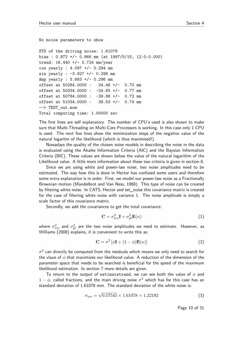
No noise parameters to show

STD of the driving noise: 1.61078

bias : 0.872 +/- 0.966 mm (at 1997/5/15, 12:0:0.000)

trend: 16.440 +/- 0.724 mm/year

cos yearly : 4.097 +/- 0.294 mm

sin yearly : -3.927 +/- 0.298 mm

Amp yearly : 5.683 +/- 0.296 mm

offset at 50284.0000 : 24.46 +/- 0.70 mm

offset at 50334.0000 : -24.65 +/- 0.77 mm

offset at 50784.0000 : -39.86 +/- 0.72 mm

offset at 51034.0000 : 38.53 +/- 0.74 mm

--> TEST_out.mom

Total computing time: 1.00000 sec

The first lines are self explanatory. The number of CPU’s used is also shown to makesure that Multi-Threading on Multi-Core Processors is working. In this case only 1 CPUis used. The next few lines show the minimization steps of the negative value of thenatural logaritm of the likelihood (which is thus maximised!).

Nowadays the quality of the chosen noise models in describing the noise in the datais evaluated using the Akaike Information Criteria (AIC) and the Baysian InformationCriteria (BIC). These values are shown below the value of the natural logarithm of theLikelihood value. A little more information about these two criteria is given in section 8.

Since we are using white and power-law noise, two noise amplitudes need to beestimated. The way how this is done in Hector has confused some users and thereforesome extra explanation is in order. First, we model our power-law noise as a FractionallyBrownian motion (Mandelbrot and Van Ness, 1968). This type of noise can be createdby filtering white noise. In CATS, Hector and est_noise this covariance matrix is createdfor the case of filtering white noise with variance 1. The noise amplitude is simply ascale factor of this covariance matrix.

Secondly, we add the covariances to get the total covariance:

C = σ2wnI + σ2

plE(κ) (1)

where σ2wn and σ2

pl are the two noise amplitudes we need to estimate. However, asWilliams (2008) explains, it is convenient to write this as:

C = σ2 [φI + (1 − φ)E(κ)] (2)

σ2 can directly be computed from the residuals which means we only need to search forthe vlaue of φ that maximizes our likelihood value. A reduction of the dimension of theparameter space that needs to be searched is beneficial for the speed of the maximumlikelihood estimation. In section 7 more details are given.

To return to the output of estimatetrend, we can see both the value of φ and1 − φ, called fractions, and the main driving noise σ2 which has for this case has anstandard deviation of 1.61078 mm. The standard deviation of the white noise is:

σwn =√

0.57545 × 1.61078 = 1.22192 (3)

of 31


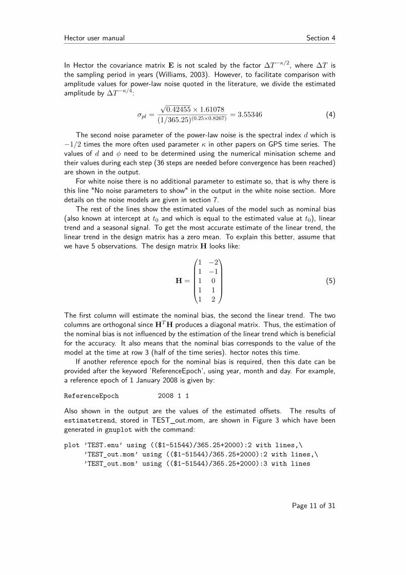
In Hector the covariance matrix E is not scaled by the factor ∆T −κ/2, where ∆T isthe sampling period in years (Williams, 2003). However, to facilitate comparison withamplitude values for power-law noise quoted in the literature, we divide the estimatedamplitude by ∆T −κ/4:

σpl =

√0.42455 × 1.61078

(1/365.25)(0.25×0.8267)= 3.55346 (4)

The second noise parameter of the power-law noise is the spectral index d which is−1/2 times the more often used parameter κ in other papers on GPS time series. Thevalues of d and φ need to be determined using the numerical minisation scheme andtheir values during each step (36 steps are needed before convergence has been reached)are shown in the output.

For white noise there is no additional parameter to estimate so, that is why there isthis line "No noise parameters to show" in the output in the white noise section. Moredetails on the noise models are given in section 7.

The rest of the lines show the estimated values of the model such as nominal bias(also known at intercept at t0 and which is equal to the estimated value at t0), lineartrend and a seasonal signal. To get the most accurate estimate of the linear trend, thelinear trend in the design matrix has a zero mean. To explain this better, assume thatwe have 5 observations. The design matrix H looks like:

H =

1 −21 −11 01 11 2

(5)

The first column will estimate the nominal bias, the second the linear trend. The twocolumns are orthogonal since HT H produces a diagonal matrix. Thus, the estimation ofthe nominal bias is not influenced by the estimation of the linear trend which is beneficialfor the accuracy. It also means that the nominal bias corresponds to the value of themodel at the time at row 3 (half of the time series). hector notes this time.

If another reference epoch for the nominal bias is required, then this date can beprovided after the keyword ’ReferenceEpoch’, using year, month and day. For example,a reference epoch of 1 January 2008 is given by:

ReferenceEpoch 2008 1 1

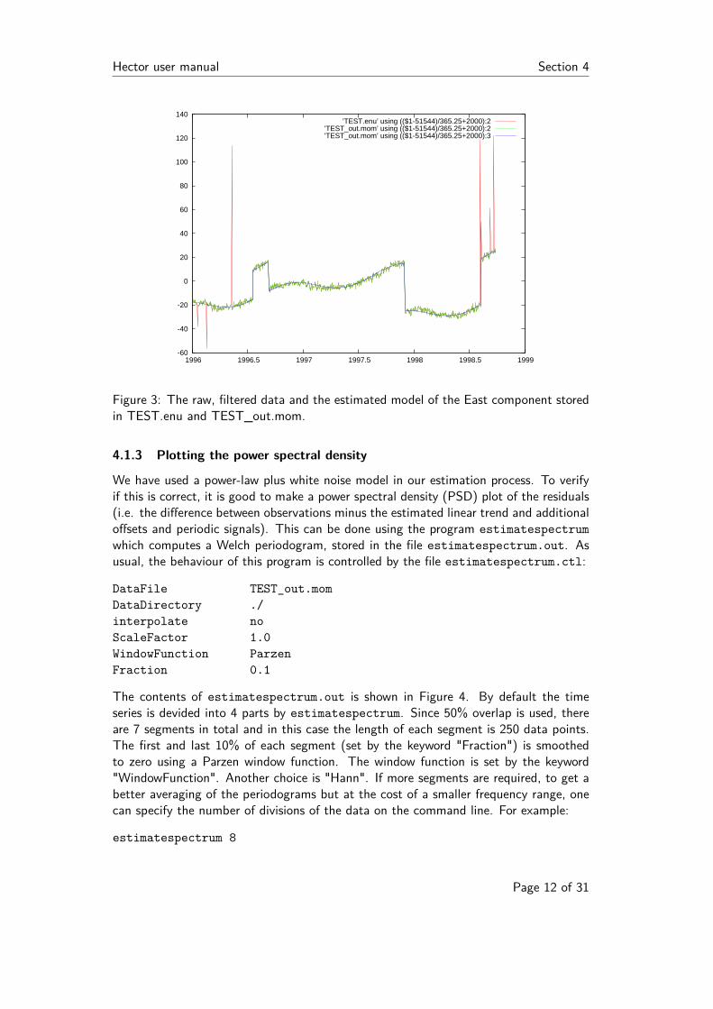
Also shown in the output are the values of the estimated offsets. The results ofestimatetrend, stored in TEST_out.mom, are shown in Figure 3 which have beengenerated in gnuplot with the command:

plot ’TEST.enu’ using (($1-51544)/365.25+2000):2 with lines,\

’TEST_out.mom’ using (($1-51544)/365.25+2000):2 with lines,\

’TEST_out.mom’ using (($1-51544)/365.25+2000):3 with lines

of 31


-60

-40

-20

0

20

40

60

80

100

120

140

1996 1996.5 1997 1997.5 1998 1998.5 1999

’TEST.enu’ using (($1-51544)/365.25+2000):2’TEST_out.mom’ using (($1-51544)/365.25+2000):2’TEST_out.mom’ using (($1-51544)/365.25+2000):3

Figure 3: The raw, filtered data and the estimated model of the East component storedin TEST.enu and TEST_out.mom.

4.1.3 Plotting the power spectral density

We have used a power-law plus white noise model in our estimation process. To verifyif this is correct, it is good to make a power spectral density (PSD) plot of the residuals(i.e. the difference between observations minus the estimated linear trend and additionaloffsets and periodic signals). This can be done using the program estimatespectrum

which computes a Welch periodogram, stored in the file estimatespectrum.out. Asusual, the behaviour of this program is controlled by the file estimatespectrum.ctl:

DataFile TEST_out.mom

DataDirectory ./

interpolate no

ScaleFactor 1.0

WindowFunction Parzen

Fraction 0.1

The contents of estimatespectrum.out is shown in Figure 4. By default the timeseries is devided into 4 parts by estimatespectrum. Since 50% overlap is used, thereare 7 segments in total and in this case the length of each segment is 250 data points.The first and last 10% of each segment (set by the keyword "Fraction") is smoothedto zero using a Parzen window function. The window function is set by the keyword"WindowFunction". Another choice is "Hann". If more segments are required, to get abetter averaging of the periodograms but at the cost of a smaller frequency range, onecan specify the number of divisions of the data on the command line. For example:

estimatespectrum 8

of 31


which will divided the time series into 8 pieces, creating 15 segments due to the 50%overlap used. The area underneath the (one-sided) power spectral density plot shouldbe equal to the variance of the time series (Buttkus, 2000). This area underneath thePSD plot has been computed by simply assuming that each point represents a bar ofwidth 1/∆t and adding them all up. Next, it is important to note the begin and endvalue of the frequency range.

************************************

estimatespectrum, version 1.6

************************************

Data format: MJD, Observations, Model

Filename : ./TEST_out.mom

Number of observations: 1000

Percentage of gaps : 10.7

window function : Parzen

window function fraction: 0.1

Number of data points n : 1000

Number of data used N : 1000

Number of segments K : 7

Length of segments L : 250

U : 0.9722

dt: 8.64e+04

scale for G to get Amplitude (mm): 0.3043

Total variance in signal (time domain): 3.313

Total variance in signal (spectrum) : 2.972

freq0: 4.6296e-08

freq1: 5.7870e-06

--> estimatespectrum.out

The PSD of our estimated noise model can be computed using the program modelspectrum

which has the control-file modelspectrum.ctl and which saves its output by defaultin modelspectrum.out. Normally one makes a PSD after estimating the trend so thisshould not be an inconvenience. The user must manually enter the requested values forthe noise parameters and provide the begin and end value of the frequency range. Forour example, the input looks like:

************************************

modelspectrum, version 1.6

************************************

Enter the standard deviation of the driving noise: 1.61078

Enter the sampling period in hours: 24

0) Powerlaw

1) White

generator type: mt19937

seed = 0

first value = 3606108063

of 31


10-3

10-2

10-1

100

100 101 102

Pow

er (

mm

2 /cpy

)

Frequency (cpy)

observedmodel

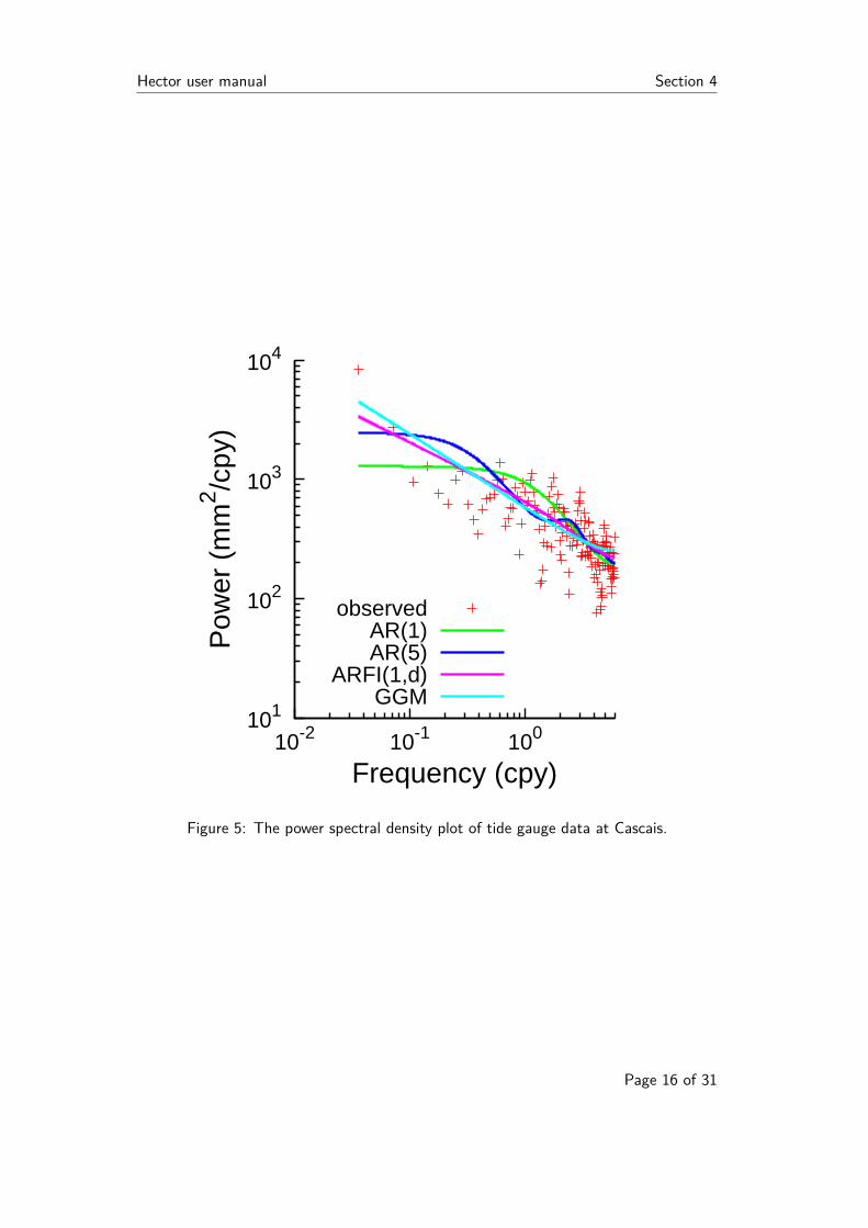
Figure 4: The PSD of the residuals and used noise model.

Enter fraction for model Powerlaw: 0.42455

Enter fraction for model White: 0.57545

Powerlaw:

Enter value of fractional difference d:0.4134

White:

1) Linear or 2) logarithmic scaling of frequency?: 2

Enter freq0 and freq1: 4.6296e-08 5.7870e-06

freq0 : 4.6296e-08

freq1 : 5.787e-06

--> modelspectrum.out

The contents of estimatespectrum.out and modelspectrum.out are plotted in Fig-ure 4.

4.2 Example 2: The monthly PSMSL tide gauge data at Cascais

In the directory ex2 we have stored the monthly tide gauge data of Cascais, downloadedfrom PSMSL (http://www.psmsl.org/data/obtaining/stations/52.php). Thistime series has no outliers so we can directly estimate the linear trend. The control-fileestimatetrend.ctl is:

DataFile 52.rlrdata

DataDirectory ./

of 31


OutputFile 52_out.mom

DegreePolynomial 1

interpolate no

seasonalsignal yes

halfseasonalsignal yes

estimateoffsets no

NoiseModels ARMA

PhysicalUnit mm

AR_p 1

MA_q 0

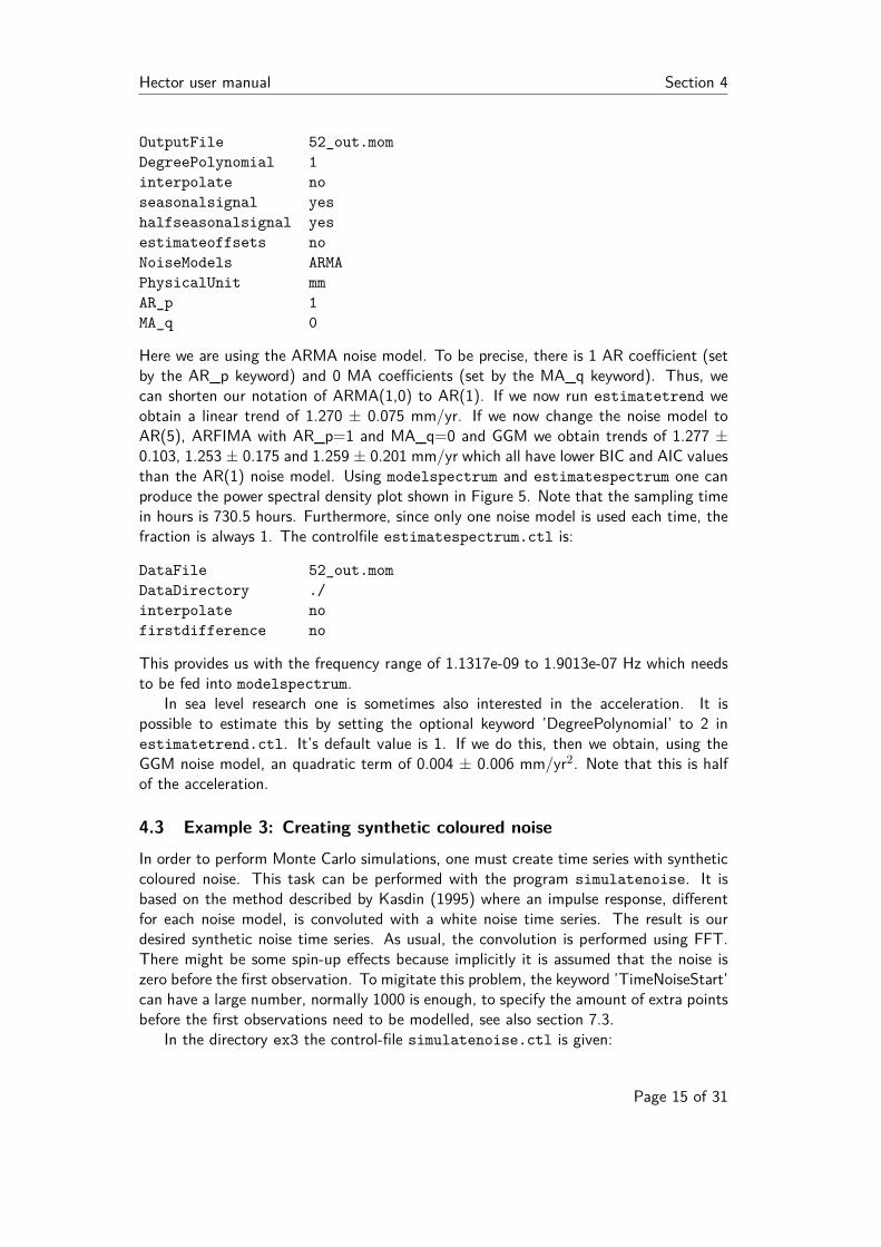
Here we are using the ARMA noise model. To be precise, there is 1 AR coefficient (setby the AR_p keyword) and 0 MA coefficients (set by the MA_q keyword). Thus, wecan shorten our notation of ARMA(1,0) to AR(1). If we now run estimatetrend weobtain a linear trend of 1.270 ± 0.075 mm/yr. If we now change the noise model toAR(5), ARFIMA with AR_p=1 and MA_q=0 and GGM we obtain trends of 1.277 ±0.103, 1.253 ± 0.175 and 1.259 ± 0.201 mm/yr which all have lower BIC and AIC valuesthan the AR(1) noise model. Using modelspectrum and estimatespectrum one canproduce the power spectral density plot shown in Figure 5. Note that the sampling timein hours is 730.5 hours. Furthermore, since only one noise model is used each time, thefraction is always 1. The controlfile estimatespectrum.ctl is:

DataFile 52_out.mom

DataDirectory ./

interpolate no

firstdifference no

This provides us with the frequency range of 1.1317e-09 to 1.9013e-07 Hz which needsto be fed into modelspectrum.

In sea level research one is sometimes also interested in the acceleration. It ispossible to estimate this by setting the optional keyword ’DegreePolynomial’ to 2 inestimatetrend.ctl. It’s default value is 1. If we do this, then we obtain, using theGGM noise model, an quadratic term of 0.004 ± 0.006 mm/yr2. Note that this is halfof the acceleration.

4.3 Example 3: Creating synthetic coloured noise

In order to perform Monte Carlo simulations, one must create time series with syntheticcoloured noise. This task can be performed with the program simulatenoise. It isbased on the method described by Kasdin (1995) where an impulse response, differentfor each noise model, is convoluted with a white noise time series. The result is ourdesired synthetic noise time series. As usual, the convolution is performed using FFT.There might be some spin-up effects because implicitly it is assumed that the noise iszero before the first observation. To migitate this problem, the keyword ’TimeNoiseStart’can have a large number, normally 1000 is enough, to specify the amount of extra pointsbefore the first observations need to be modelled, see also section 7.3.

In the directory ex3 the control-file simulatenoise.ctl is given:

of 31


101

102

103

104

10-2 10-1 100

Pow

er (

mm

2 /cpy

)

Frequency (cpy)

observedAR(1)AR(5)

ARFI(1,d)GGM

Figure 5: The power spectral density plot of tide gauge data at Cascais.

of 31


SimulationDir ./

SimulationLabel test_base

NumberOfSimulations 10

NumberOfPoints 5000

SamplingPeriod 1

TimeNoiseStart 1000

NoiseModels Flicker White

PhysicalUnit mm

Some of these keywords are new. For example, ’SimulationDir’ specifies in which di-rectory the created files should be stored. The keyword ’SimulationLabel’ specifies thebase name of those files. The next keyword tells hector how many simulation runs arerequired. The filenames will in this case be: test_base0.mom, test_base1.mom, . . .,test_base9.mom.

The keyword ’NumberOfPoints’ specifies the number of points in the the time seriesand the keyord ’TimeNoiseStart’ was already discussed above.

When simulatenoise is run, it will ask the user to manually enter the parametervalues of the chosen noise model. In this case it will ask the values of φ and d.

4.4 Example 4: Estimating amplitude of post-seismic relaxation

Nowadays one also would like to model the post-seismic part of the station motion afteran earthquake. We allow both an exponential and logarithmic model, see subsection5.1. In directory ex4 a simple example is given.

4.5 Example 5: Including extra geophysical signals for multivariate anal-

ysis

Suppose one has the temperature of the GNSS pillar and want to see if this corre-lates with the variations of the vertical position of the GNSS station. To includethis additional geophysical signal in the time series analysis, one has to set the labelestimatemultivariate to yes in estimatetrend.ctl. In addition one must give thename of the file with the geophysical signal after the keyword MultiVariateFile, alsoin estimatetrend.ctl. This multivariate has time, in modified Julian Date, in thefirst column. Note that these should be exactly the same as the MJD values in theobservation file. Columns 2 to N should contain the geophysical signals one want toinclude. In the output the estimated scale factors are shown. In ex5 a simple exampleis given.

4.6 Example 6: Estimating multilinear trends

In some cases, it seems as if the linear trend is different before and after an earthquake.To model that, you have to set the keyword estimatemultitrend in estimatetrend.ctl.In directory ex6 a simple example is given.

of 31


5 Model specification

We assume that the observations are the sum of a deterministic model and stochasticnoise. This deterministic model is (Bevis and Brown, 2014):

x =nP∑

i=0

pi(t − tR)i +nJ∑

i=1

bjH(t − tj)

+nF∑

i=1

si sin(ωit) + ci cos(ωit)

+nT∑

i=1

ei(1 − exp(−(t − ti)/Ti))+

+nL∑

k=1

ak log(1 + (t − tk)/Tk))

(6)

where pi are the coefficients of a nP degree polynomial. By default nP = 1: a lineartrend. Following convention, we give the rate in unit per year, where a year is defined as365.25 days. Note that acceleration is normally defined to be twice the quadratic term.

H(t) is the Heaviside step function and used to model offsets with amplitudes bj .An annual and semiannual signal are commonly included in the model and therefore

have their own keywords ’seasonal’ and ’halfseasonal’. In the equation their angularvelocities are represented by ωi Other periodic signals need to be entered using thekeyword ’PeriodicSignals’, followed by a list of their periods in days.

It is often desired to speak about the amplitude of the annual and semi-annualperiod. To facilitate this, Hector shows also this parameter. It has been computedby first assuming a mean uncertainty for si and ci which we call σ. In this case theamplitude follows a Rice distribution with a mean of σ

√

π/2 L1/2(−ν2/(2σ2)) where

ν =√

c2i + s2

i and L1/2(x) = 1F1(−1/2, 1, x).

5.1 Post-seismic deformation

Since version 1.6 one can also include post-seismic deformation in the model by extendingthe header of the data file by adding lines that contain the time when the relaxationstarts (in MJD) and the relaxation period in days. An example is:

# log 51994.0 10.0

# log 55044.0 10.0

# exp 53544.0 100.0

One can use an exponential or logarithmic function, see Eq. 6. To estimate thesepost-seismic relaxations, one must set the keyword ’estimatepostseismic’ to yes in esti-matetrend.ctl. Note that one cannot chose between East, North or Up component. Itis applied to all if a file with more than one component is used.

of 31


5.2 Multi-trend

So far we have assumed that there is only one linear trend in the time series. However, ithas become clear that some GNSS time series show a different linear trend after a majorearthquake. To estimate different linear trends in a single time series, one can replacethe polynomial trend with the following:

p0 +M∑

k=1

p1k(ti − bk)(H(ti − bk) − H(ti − bk+1)) (7)

where p1k is now the linear trend value for each segment k. We assume that there are Msegments and the first epoch of each segment k is denoted by bk. H(t) is the Heavisidestep function.

Since the velocites are now not the same over the whole time series, the concept ofa "reference epoch" loses its utility because one can no longer define the realisation ofa reference frame as a set of positions and a single set of velocities. The concept oftrajectory models of Bevis and Brown (2014) becomes more convenient.

Another implication is that the size of the estimated offsets become dependend onthe size of the linear trend. Hector corrects for this when showing the values on thescreen. And, using propagation of errors, the uncertainty in the trend value at the endof segment k is added to the uncertainty of the estimated offset between segment k andk + 1.

The time of a break in the linear trend is given in the header of the time series.Assuming that the two earthquake mentioned in the previous example were accompaniedby a change in linear trend in the north and east component, then this is indicated by:

# break 51994.0 0

# break 51994.0 1

The indication of the component is not required if a file with only one component isused.

To estimate multi-trends, one must set the keyword ’estimatemultitrend’ to yes inestimatetrend.ctl.

6 Acceptable data format

Hector can accept various data formats which are described in this section. All of theare plain ASCII files and the time should always be increasing and the time step shouldbe constant. The data format is specified by the extension of the filename. For example,the file name TEST.enu has the extension ’enu’.

For the mom and enu-format, the sampling period in days can be specified in theheader as follows:

# sampling period 1.0

If this information is missing, then hector tries to estimate the sampling period from thefirst few observations. The sampling periods it can detect automatically are: 0.5 hour,1 hour, 1 day and 7 days. Note that this sampling period must always be given in days!

of 31


6.1 mom-format

This format expects 2 or 3 columns. The first column contains the time in MJD, thesecond the Observations. The third column is optional and should contain the estimatedModel. Missing data are allowed.

6.2 enu-format

This format is similar to the mom-format but has four columns. The first columncontains the time in MJD, the second to the fourth column contain the East, North andUp component. Missing data are allowed.

6.3 neu-format

This format is used by SOPAC (http://sopac.ucsd.edu/) and accepted by the CATSsoftware. The first column contains the time as year-fractions and columns two to fourcontain the North, East and Up component in metres. Missing data are allowed. The unitof these files is normally metres and it is convenient to convert these to millimetres usingthe keyword ScaleFactor in removeoutliers.ctl. The year-fractions are convertedinside Hector to MJD using the formula:

MJD = floor(365.25 ∗ (T − 1970) + 40587 + 0.1) − 0.5 (8)

This implies that only sampling periods which are an integer multiple of 1 day areacceptable. Hector can read the slightly different offset headers which are of the form,see the CATS manual (Williams, 2008):

# offset 2003.45479 7

Note however that if an external file with offset information is used, then the expectedformat is of the form day-month-year NaN NaN NaN. where the last three parametersstand for East, North and Up. NaN indicates that an offset needs to be estimated. Anormal number such as 0, tells the program not offset needs to be estimated for thatcomponent.

6.4 rlrdata-format

Hector can read PSMSL’s monthly data format, see http://www.psmsl.org/. Tocreate an evenly spaced data set inside Hector, each month is assumed to take exactly30.4375 days, equal to 730.5 hours.

7 Implemented Noise Models

Hector can use various types of noise models and in addition, accepts various combi-nations of them with power-law plus white noise being the most popular for GPS timeseries. Williams (2008) wrote the covariance matrix C of this particular combination as:

C = σ2(

cos2 φ I + sin2 φ E(d))

(9)

of 31

http://sopac.ucsd.edu/

http://www.psmsl.org/


where I is the unit matrix (equal to the covariance matrix for unit white noise) and E

the covariance matrix for power-law noise which depends on the spectral index d. Thedistribution of the magnitudes of both noise models is controlled by the parameter φ.The total variance of the noise is set by σ2 (This is called the ’driving’ noise in theoutput). This has been generalized to:

C = σ2 (φ1E1 + (1 − φ1)φ2E2 + (1 − φ1)(1 − φ2)φ3E3 + . . .

(1 − φ1)(1 − φ2) . . . φN EN+1) (10)

for N +1 noise models. All φ-parameters vary between 0 and 1. As was noted in section1, only stationary noise is accepted. This creates a Toeplitz covariance matrix and onlythe first column of the covariance matrix needs to be stored. This column vector will bedenoted by γ.

7.1 White noise

For white noise the covariance matrix is just the unit matrix The first column of thecovariance matrix C, with σ = 1, is:

γi = 1 for i = 0 (11)

= 0 i 6= 0 (12)

Its one-sided power spectrum density is:

S(f) = 21

fs(13)

where fs is the sampling frequency in Hz. If you integrate this from zero frequency tothe Nyquist frequency, you get the variance that is observed in the time series, as itshould be.

7.2 Power-law noise

For power-law noise the first column of the covariance matrix is:

γi =Γ(d + i)Γ(1 − 2d)

Γ(d)Γ(1 + i − d)Γ(1 − d)(14)

Its one-sided power spectrum density, with σ = 1, is:

S(f) = 21

fs

1

(2 sin(πf/fs))2d(15)

7.3 Power-law approximated

Bos et al. (2013) introduced a Toeplitz approximation for power-law noise which can bechosen using the label "PowerlawApprox" after the keyword Noisemodels. In addition,one must specify the number of days before the start of the observation when the noiseis assumed to have started after the keyword "TimeNoiseStart". A value of 1000 is agood first guess. Note that nowadays we prefer to use the Generalized Gauss Markovnoise model with φ close to 1. This also approximates power-law noise and works betterfor spectral indices smaller than -1.

of 31


7.4 ARFIMA and ARMA

The definition of the ARFIMA noise model is Sowell (1992):

Φ(L)(1 − L)dzt = Θ(L)ǫt (16)

L is the backshift operator (Lxi = xi−1), zt is the residual at time t (observation minusmodelled signal) and ǫ is a white noise signal. In other words, Eq. (16) says that theresiduals in the observations can be produced by applying some transformations on awhite noise process. The operators Φ and Θ are defined as, see Hosking (1981):

Φ(L) = 1 − φ1L − φ2L2 − . . . − φpLp (17)

Θ(L) = 1 + θ1L + θ2L2 + . . . + θqLq (18)

This definition is implemented in Hector but note that the definition of the signs beforethe φ coefficients in Φ are positive in Sowell (1992). To complicate matters further, thecoefficients of Θ are negative in the formula’s of Zinde-Wash (1988).

The value of the integers p and q are set by the keywords AR_p and MA_q respec-tively in estimatetrend.ctl. It is advised to use values for p smaller than 5 to ensurethat the MLE procedure always start with coefficients values for φ1, . . . , φp of Φ(L) thatproduce stationary noise. If p and q are zero, then one obtains again a pure power-lawnoise process. We have implemented the method of Doornik and Ooms (2003) to com-pute the first column of the covariance matrix. For the special case when d = 0, we usethe equations of Zinde-Wash (1988) and can be selected by using the name ’ARMA’after the keyword Noisemodels. For sea level research the first order auto-regressive noisemodel is a popular choice: ARMA(1,0). For pure ARMA noise models faster MaximumLikelihood Methods exist, see for example Brockwell and Davis (2002), but Hector willgive the same result. To specify AR(1) in ’estimatetrend.ctl’ one must write:

NoiseModels ARMA

AR_p 1

MA_q 0

7.5 Generalized Gauss Markov noise model

Langbein (2004) took the first order Gauss Markov noise model depending on the pa-rameter φ and modified with an additional parameter, d, to create power-law noise witha slope of 2d in the power density spectrum which flattens to white noise at the verylow and very high frequencies. The analytical expression for the autocovariance vector(with σ = 1) for this noise model is:

γi =Γ(d + i)(1 − φ)i

Γ(d)Γ(1 + i)2F1(d, d + i; 1 + i; (1 − φ)2) (19)

This noise model can be used using the name ’GGM’ after the keyword Noisemodels inestimatetrend.ctl. Bos et al. (2014) provide some additional formula’s.

The 1 − φ parameter can be held fixed a priori by adding to the control-file:

GGM_1mphi XXXX

where XXXX is the value you want to give this parameter. 6.881e-06 is normally smallenough. If it is small enough, then GGM approximates a pure power-law model.

of 31


7.6 Flicker noise and Random Walk noise

Flicker noise and Random walk noise are simply two types of power-law noise where thespectral index d has the fixed value of 0.5 and 1.0 respectively. However, as was notedin the introduction, Hector can only deal with stationary noise because that results inToeplitz covariance matrices that allow fast inversion techniques. As will be explained ina future publication, this can be achieved by using the Generalized Gauss Markov noisemodel with a small value for the 1 − φ parameter. For example:

NoiseModels FlickerGGM

GGM_1mphi 6.881e-06

8 The Akaike and Baysian Information Criteria

Hector allows the estimation of linear trend or a higher order polynomial, seasonal andother periodic signals and a variety of noise models which can be combined. To chose thebest model one can make use of the Akaike or Baysian Information Criteria (Akaike, 1974;Schwarz, 1978). Both use the log-likelihood as their starting point but add penalties foradding parameters in order to avoid overfitting.

The definition of the log-likelihood is:

ln(L) = −1

2

[

N ln(2π) + ln det(C) + rT C−1r]

(20)

where N is the actual number of observations (gaps do not count). The covariancematrix C is decomposed as:

C = σ2C̄ (21)

where C̄ is the sum of various noise models and σ the standard deviation of the ’driving’white noise process as was explained in section 7. σ is estimated from the residuals:

σ =

√

rT C̄−1r

N(22)

Using this relation and the fact that det cA = cN det A, the following formulation forthe likelihood is implemented:

ln(L) = −1

2

[

N ln(2π) + ln det(C̄) + 2N ln(σ) + N]

(23)

The number of parameters k is the sum of parameters in the Design matrix H andthe noise models and the variance of the driving white noise process. For example,for estimating a linear trend using power-law + white noise models 5 parameters areinvolved: nomial bias, linear trend, distribution of variances between power-law andwhite noise, spectral index of the power-law and the variance of the driving white noiseprocess (k = 2 + 2 + 1 = 5).

The Akaike Information Criterion (AIC) and Baysian Information Criterion (BIC) aredefined as:

AIC = 2k + 2 ln(L) (24)

BIC = k ln(N) + 2 ln(L) (25)

of 31


The preferred model is the one with the minimum AIC/BIC value. Note that these arerelative measures between various choices, not absolute criteria.

9 Quick reference for the control-files

9.1 removeoutliers.ctl

This file is read by removeoutliers.

Keyword Value(s)

DataFile name of file with observationsDataDirectory directory where file with observations is storedOffsetFile name of file with offset information (optional)OutputFile name of file with observations and estimated model in

.mom formatcomponent only required for the .enu and .neu format or when an

OffsetFile is being used. Select East, North or Upinterpolate yes|noDegreePolynomial degree of polynomial: 0-6, (optional, default=1)estimatemultitrend yes|no (optional, default=no. If yes, then DegreePoly-

nomail keyword is ignored. Only linear trends are esti-mated)

estimatepostseismic yes|no (optional, default=no)seasonalsignal yes|nohalfseasonalsignal yes|noperiodicsignals a sequence of numbers reprenting the period in days (op-

tional)estimateoffsets yes|noScaleFactor a number to scale the observations (optional, default=1)PhysicalUnit the physical unit of the observationsIQ_factor the number used to scale the interquartile range

9.2 estimatetrend.ctl

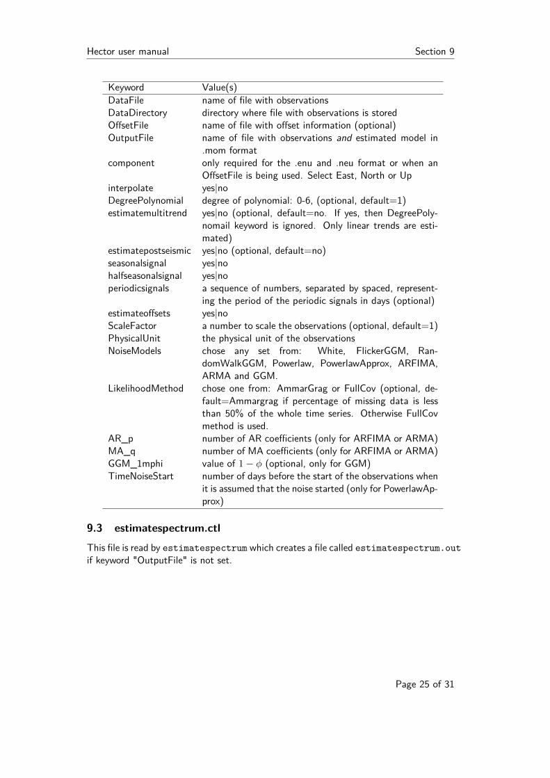
This file is read by estimatetrend and by modelspectrum although the latter onlyreads the keyword NoiseModels and, if necessary, the keywords AR_p, MA_q andTimeNoiseStart. The program modelspectrum creates a file called modelspectrum.out.

of 31


Keyword Value(s)

DataFile name of file with observationsDataDirectory directory where file with observations is storedOffsetFile name of file with offset information (optional)OutputFile name of file with observations and estimated model in

.mom formatcomponent only required for the .enu and .neu format or when an

OffsetFile is being used. Select East, North or Upinterpolate yes|noDegreePolynomial degree of polynomial: 0-6, (optional, default=1)estimatemultitrend yes|no (optional, default=no. If yes, then DegreePoly-

nomail keyword is ignored. Only linear trends are esti-mated)

estimatepostseismic yes|no (optional, default=no)seasonalsignal yes|nohalfseasonalsignal yes|noperiodicsignals a sequence of numbers, separated by spaced, represent-

ing the period of the periodic signals in days (optional)estimateoffsets yes|noScaleFactor a number to scale the observations (optional, default=1)PhysicalUnit the physical unit of the observationsNoiseModels chose any set from: White, FlickerGGM, Ran-

domWalkGGM, Powerlaw, PowerlawApprox, ARFIMA,ARMA and GGM.

LikelihoodMethod chose one from: AmmarGrag or FullCov (optional, de-fault=Ammargrag if percentage of missing data is lessthan 50% of the whole time series. Otherwise FullCovmethod is used.

AR_p number of AR coefficients (only for ARFIMA or ARMA)MA_q number of MA coefficients (only for ARFIMA or ARMA)GGM_1mphi value of 1 − φ (optional, only for GGM)TimeNoiseStart number of days before the start of the observations when

it is assumed that the noise started (only for PowerlawAp-prox)

9.3 estimatespectrum.ctl

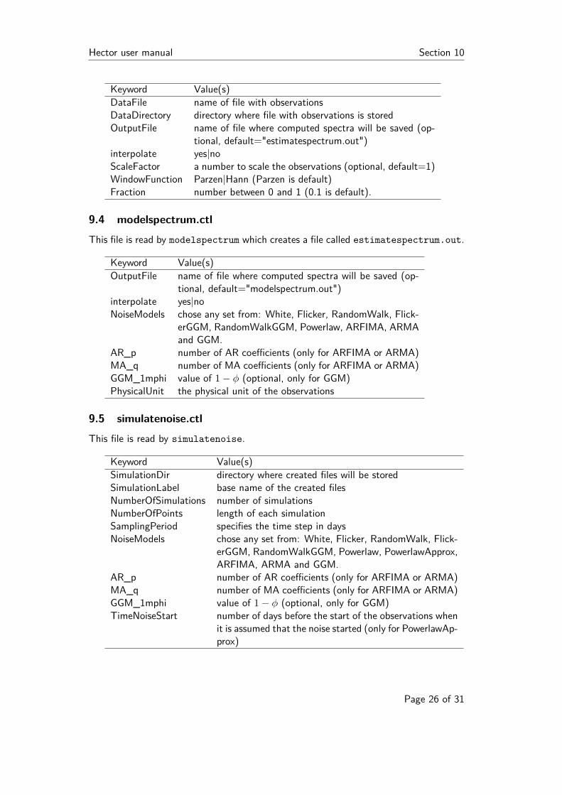
This file is read by estimatespectrum which creates a file called estimatespectrum.out

if keyword "OutputFile" is not set.

of 31


Keyword Value(s)

DataFile name of file with observationsDataDirectory directory where file with observations is storedOutputFile name of file where computed spectra will be saved (op-

tional, default="estimatespectrum.out")interpolate yes|noScaleFactor a number to scale the observations (optional, default=1)WindowFunction Parzen|Hann (Parzen is default)Fraction number between 0 and 1 (0.1 is default).

9.4 modelspectrum.ctl

This file is read by modelspectrum which creates a file called estimatespectrum.out.

Keyword Value(s)

OutputFile name of file where computed spectra will be saved (op-tional, default="modelspectrum.out")

interpolate yes|noNoiseModels chose any set from: White, Flicker, RandomWalk, Flick-

erGGM, RandomWalkGGM, Powerlaw, ARFIMA, ARMAand GGM.

AR_p number of AR coefficients (only for ARFIMA or ARMA)MA_q number of MA coefficients (only for ARFIMA or ARMA)GGM_1mphi value of 1 − φ (optional, only for GGM)PhysicalUnit the physical unit of the observations

9.5 simulatenoise.ctl

This file is read by simulatenoise.

Keyword Value(s)

SimulationDir directory where created files will be storedSimulationLabel base name of the created filesNumberOfSimulations number of simulationsNumberOfPoints length of each simulationSamplingPeriod specifies the time step in daysNoiseModels chose any set from: White, Flicker, RandomWalk, Flick-

erGGM, RandomWalkGGM, Powerlaw, PowerlawApprox,ARFIMA, ARMA and GGM.

AR_p number of AR coefficients (only for ARFIMA or ARMA)MA_q number of MA coefficients (only for ARFIMA or ARMA)GGM_1mphi value of 1 − φ (optional, only for GGM)TimeNoiseStart number of days before the start of the observations when

it is assumed that the noise started (only for PowerlawAp-prox)

of 31


10 Advanced Features

10.1 Offsets

The information about the time of an offset can also be provided in an another fileinstead of in the header of the file with the observations. In this case one must specifythe keyword ’OffsetFile’ and its name in the control-file. One must also not forget tospecify the component in the control-file. Since most people prefer simple day-month-year format, the format for the offsets in the external file is a bit different. Using theoffset data shown before, we have:

20- 7-1996 NaN 0 0

8- 9-1996 NaN NaN 0

2-12-1997 NaN 0 0

9- 8-1998 NaN 0 0

This external file with time of offsets can be used with removeoutliers andestimatetrend.

11 License and Copyright

Hector is Copyright © 2012-1016 Machiel Bos, Rui Fernandes and Luísa Bastos.Hector is free software; you can redistribute it and/or modify it under the terms of

the GNU General Public License as published by the Free Software Foundation; eitherversion 2 of the License, or (at your option) any later version.

This program is distributed in the hope that it will be useful, but WITHOUT ANYWARRANTY; without even the implied warranty of MERCHANTABILITY or FITNESSFOR A PARTICULAR PURPOSE. See the GNU General Public License for more details.

You should have received a copy of the GNU General Public License along with thisprogram; if not, write to the Free Software Foundation, Inc., 51 Franklin Street, FifthFloor, Boston, MA 02110-1301 USA You can also find the GPL on the GNU web site.

References

Agnew, D. C. (1992). The time-domain behaviour of power-law noises. Geophys. Res.

Letters, 19(4):333–336.

Akaike, H. (1974). A new look at the statistical model identification. IEEE Transactions

on Automatic Control, 19(6):716–723.

Beran, J. (1992). Statistical methods for data with long-range dependence. Statistical

Science, 7(4):404–416.

Bevis, M. and Brown, A. (2014). Trajectory models and reference frames for crustalmotion geodesy. Journal of Geodesy, 88:283–311.

Bos, M. S., Fernandes, R. M. S., Williams, S. D. P., and Bastos, L. (2013). Fast ErrorAnalysis of Continuous GNSS Observations with Missing Data. J. Geod., 87(4):351–360.

of 31

Hector user manual Section A

Bos, M. S., Williams, S. D. P., Araújo, I. B., and Bastos, L. (2014). The effect of tem-poral correlated noise on the sea level rate and acceleration uncertainty. Geophysical

Journal International, 196:1423–1430.

Brockwell, P. and Davis, R. A. (2002). Introduction to Time Series and Forecasting.Springer-Verlag, New York, second edition edition.

Buttkus, B. (2000). Spectral Analysis and Filter Theory in Applied Geophysics. Springer-Verlag Berlin Heidelberg.

Doornik, J. A. and Ooms, M. (2003). Computational Aspects of Maximum LikelihoodEstimation of Autoregressive Fractionally Integrated Moving Average Models. Com-

putational Statistics and Data Analysis, 42:333–348.

Hosking, J. R. M. (1981). Fractional differencing. Biometrika, 68:165–176.

Kasdin, N. J. (1995). Discrete simulation of colored noise and stochastic processes and1/fα power-law noise generation. Proc. IEEE, 83(5):802–827.

Langbein, J. (2004). Noise in two-color electronic distance meter measurements revisited.J. Geophys. Res., 109(B04406).

Langbein, J. (2010). Computer algorithm for analyzing and processing borehole strain-meter data. Computers & Geosciences, 36(5):611–619.

Langbein, J. and Bock, Y. (2004). High-rate real-time GPS network at Parkfield: Utilityfor detecting fault slip and seismic displacements. Geophys. Res. Letters, 31:15.

Mandelbrot, B. B. and Van Ness, J. W. (1968). Fractional Brownian motions, fractionalnoises and applications. SIAM-REVIEW, 10(4):422–437.

Schwarz, G. (1978). Estimating the Dimension of a Model. The Annals of Statistics,6(2):461–464.

Sowell, F. (1992). Maximum likelihood estimation of stationary univariate fractionallyintegrated time series models. J. Econom., 53:165–188.

Williams, S. D. P. (2003). The effect of coloured noise on the uncertainties of ratesfrom geodetic time series. J. Geod., 76(9-10):483–494.

Williams, S. D. P. (2008). CATS : GPS coordinate time series analysis software. GPS

Solutions, 12(2):147–153.

Zinde-Wash, V. (1988). Some Exact Formulae for Autoregressive Moving Average Pro-cesses. Econometric Theory, 4(3):384–402.

of 31


A History of changes made in the various versions of

Hector

A.1 Version 1.1

1. The programs estimatetrend, removeoutliers, estimatespectrum and modelspectrum

now accept the name of the control-file on the command line. For example:

estimatetrend mycontrol.ctl

2. The date of the nominal bias of the whole time series can now be set in estimate-trend.ctl using the keyword ’ReferenceEpoch’. Furthermore, in the output this dateis now shown in "day/month/year hour" format instead of Modified Julian Date.If this keyword is not provided, then the default behaviour is to define the Refer-enceEpoch as the midpoint between the start and end time of the observations.

3. The ability to leave out a keyword also made it possible to define other defaultparameters. Now it is no longer necessary to provide the ScaleFactor keyword ifthis is not different from 1 and the LikelihoodMethod keyword is optinal. If it ismissing, then the AmmarGrag method will be used when the amount of missingdata is less than 50% of the whole time series. Otherwise the FullCov method isused.

4. The ARFIMA model had two bugs, one due to a sign error and one due to accessingarrays outside their range, which have been resolved.

5. The keyword ’MinimizingMethod’ has been removed because the Nelder-MeadSimplex method is the only method available.

6. The header information about the sampling period and the time of offsets can nowbe given in a separate file using the keyword ’OffsetFile’.

7. It is now also possible to estimate a quadratic polynomial by setting the keyword’QuadraticTerm’ to yes.

8. The program simulatenoise was added.

9. Implemented the dd-mm-year NaN NaN NaN offset format for external files.

A.2 Version 1.2

1. simulatenoise has now correct power.

2. The ARMA and ARFIMA noise model now also accept first-difference (removedfrom version 1.5 onwards).

3. All programs now except ridiculously long names.

of 31


A.3 Version 1.3

1. Removed a bug which caused Hector to crash on some computers. The reasonwas that Nnumbers was not set to zero explicitly.

2. The parser of the control-files had trouble when there was a space after the lastlabel. For example "NoiseModels PowerlawApprox White " where there is a spacebehind the last word. This has now hopefully been corrected in Control.cpp

3. Using the Generalized Gauss Markov noise model did not converge in rare situationsbut they did occur. Now the maximum value of φ has been lowered from 0.9999to 0.999. (has been solved in version 1.6 and now the limit is closer to 0.999999)

4. The binaries are now stored in /usr/local/bin instead of /usr/bin which wehope is more following the Linux standard.

A.4 Version 1.4

1. Better command line parsing for estimatespectrum.

2. Added "# sampling period 1.0" in .enu file created by convert_sol_files.tcl.

3. Removed root-message in ARFIMA.cpp.

4. Removed trailing spaced bug in Control.cpp (again).

5. Improved C++ correctness (fp.getline(..)!=NULL) in Observations.cpp

A.5 Version 1.5

1. Removed the option to apply first difference to data. This option was never usedand it makes the source code unnecessary complicated.

2. Added Hann window to estimatespectrum. You can now chose between theHann and Parzen window function and select the percentage of data to which thiswindow will be applied at both ends of the segment.

3. Implemented a Taylor expansion of the Hypergeometric function in GenGauss-Markov.cpp and now φ can be closer to 1: 0.9999. This helps to simulate purepower-law noise.

4. Changed the output of estimatetrend by elminating parameters d, driving noiseand fractions. The noise amplitudes now follow CATS.

5. The Plate Boundary Observatory changed their time series file format. We find iteasier to write a little script to convert the new format to my mom-format thanto update the Observations.cpp class.

6. Removed subsection "Some additional tests" since it was not read or createdconfusion for those who did.

of 31


A.6 Version 1.5.1

1. Removed a small bug in the class Minimizer.cpp that left the first parameter 0.001larger than the optimal value (residual of computing Fisher information matrix).It had a large effect if "Random Walk" was the first chosen noise model.

2. Added to the manual that you can set the 1 − φ value a priori in the control-file.

A.7 Version 1.5.2

1. Still problem of having spaces in list of items in Control.cpp which now hopefullyhas been solved.

A.8 Version 1.6

1. Introduced logarithmic and exponential post-seismic relaxation in Designmatrix.

2. Generalised linear and quadratic trend to N degree polynomial. To keep mainte-nance simple, I removed the ’QuadraticTerm’ keyword.

3. Number of allowed periodical signals in the estimation process has been increasedfrom 20 to 40.

4. One can select to estimate multi linear trends instead of a singly polynomial.

5. estimatespectrum and modelspectrum now allow the keyword "OutputFile" toredirect their output to another file. Note that now the default control-file formodelspectrum is modelspectrum.ctl to be consistent.

6. Removed memory leaks.

7. Added multivariate analysis option.

8. Added multi-trend option.

9. Added polynomial option.

10. Added post-seismic model option.

of 31

Hector user manual version 1 - Welcome to SEGALsegal.ubi.pt/hector/manual_1.6.pdf · Hector is...

Documents

Transcript of Hector user manual version 1 - Welcome to SEGALsegal.ubi.pt/hector/manual_1.6.pdf · Hector is...