HEC Montréal Analysis of Inventory Levels of Canadian ...party logistics, information technology,...

1

HEC Montréal

Analysis of Inventory Levels of Canadian Companies

By

Nitin Ravishankar (11193393)

M.Sc. Administration

Global Supply Chain Management

Thesis submitted in Partial Fulfilment of the

Requirements for the Degree of

Master of Science (M.Sc.)

December 2016

© Nitin Ravishankar, 2016

3

Résumé

La philosophie du juste-à-temps et de la fabrication sans gaspillage a mené les entreprises à la

poursuite des politiques pour minimiser les stocks. En même temps, la variété croissante des

produits, des niveaux de service à la clientèle plus élevés et l’incertitude de la demandes

requièrent beaucoup de stocks. En général, les études qui examinent les entreprises

manufacturières aux États-Unis révèlent une diminution du niveau des stocks, mais celles qui

enquêtent sur les entreprises américaines du secteur de gros et de détail montrent soit des

résultats contradictoires, soit aucune tendance. En plus, les recherches faites sur les entreprises

hors de l’économie américaine montrent une baisse marginale pour les entreprises situées dans

les grandes économies et aucun impact précis pour les entreprises situées dans des plus petites

économies. L'objectif de ce mémoire est d'analyser l’évolution des niveaux de stocks des

entreprises canadiennes. Aucune recherche de ce genre n'a été trouvée dans notre revue de la

littérature. Les résultats d’une analyse des séries chronologiques sur les données de 420

entreprises cotées en bourse au Canada indiquent que les niveaux de stocks mesurés par le taux

rotation des stocks des entreprises canadiennes cotées en bourse ont diminué pour la période de

1987 à 2016. Cette diminution a été trouvée dans le stock net ainsi que dans toutes les trois

catégories de stocks - matières premières, travaux en cours, et stocks des produits finis. Les

modèles utilisés dans cette étude expliquent entre 70,23% et 78,07% des variations des variables

dépendantes. En plus, la corrélation du niveau de stock net avec la marge brute, la taille de

l'entreprise, l'investissement dans les immobilisations et la croissance des ventes sont également

examinés. Seule la marge brute montre une corrélation positive avec les niveaux de stocks

relatifs, tandis que la croissance des ventes et la taille de l'entreprise montrent une corrélation

négative avec les niveaux de stocks relatifs. Nous ne trouvons pas de relation statistiquement

4

significative entre l'investissement dans les immobilisations et les niveaux de stocks des

entreprises canadiennes.

5

Abstract

The just-in-time (JIT) and lean philosophy led companies to pursue policies to minimize

inventory. However, increasing product variety, higher customer service levels and demand

uncertainty require larger inventories. We hence observe two opposing tendencies. Utilizing

relative inventory level measures, previous studies investigating manufacturing sector firms in

the U.S. show some level of decline in inventories but those investigating the U.S. wholesale and

retail sector firms either give conflicting results or show no trend. In addition, research carried

out for firms in non-U.S. economies show a marginal decline for firms in larger economies and

no clear cut impact for those in smaller economies. The aim of this thesis is to analyze inventory

levels specifically in Canadian companies. No such research has been found in our literature

review. Performing a time series analysis on the data of 420 publicly listed firms in Canada, the

results indicate that the relative inventory levels of the publicly listed Canadian firms measured

in terms of inventory turnover have been declining for the period from 1987 to 2016. The decline

has been found for net inventory as well as for the work-in-progress inventories. The models

used in the current study explain about 70.23% to 78.07% of the variation in the dependent

variables. In addition, the correlation of the net inventory with the gross margin, firm size,

investment in fixed assets and growth in sales are also examined. Among these factors, gross

margin shows a positive correlation with the relative inventory levels while sales growth and

firm size show a negative correlation with relative inventory levels. No statistically significant

relation was found between investment in fixed assets and inventory levels of the Canadian

companies.

6

Acknowledgement

I would like to thank my supervisors at HEC Montreal, Dr. Claudia Rebolledo and Dr. Raf Jans

for their constant guidance and inputs right from the beginning. It would not have been possible

to accomplish the research without their support and counsel. I want to thank Dr. Jean-François

Plante for providing useful insights and clarifications for statistical inferences.

I would also like to thank the librarians working in the Myriam et J.-Robert Ouimet Library at

HEC Montreal for helping me initially while searching for the databases of the public Canadian

companies.

7

Content

Résumé ............................................................................................................................................ 2

Abstract ........................................................................................................................................... 5

Acknowledgement .......................................................................................................................... 6

List of Tables & Figures ............................................................................................................... 10

List of Acronyms .......................................................................................................................... 11

1 Introduction ................................................................................................................................ 12

2 Literature review ........................................................................................................................ 15

2.1 Five major studies – U.S. .................................................................................................... 17

2.2 Factors impacting inventory trends – U.S. .......................................................................... 22

2.2.1 Firm size ....................................................................................................................... 27

2.2.2 Globalization ................................................................................................................ 28

2.2.3 JIT & lean systems ....................................................................................................... 30

2.2.4 Industry ......................................................................................................................... 32

2.2.5 IT investments .............................................................................................................. 34

2.2.6 Competition, profit margin & industry concentration .................................................. 35

2.2.7 Unique response variable – Fixed weight Inventory to sales ratio ............................... 36

2.2.8 Inventory trend and financial impact ............................................................................ 37

2.2.9 Discussion ..................................................................................................................... 38

2.3 Non-U.S. studies and discussion ......................................................................................... 39

8

2.3.1 Non-U.S. studies .............................................................................................................. 40

2.3.2 Discussion & Conclusion ................................................................................................ 42

3 Research Objective and hypotheses ........................................................................................... 44

3.1 Research Objective .............................................................................................................. 44

3.2 Hypotheses .......................................................................................................................... 44

4 Methodology .............................................................................................................................. 48

4.1 Database and variables ........................................................................................................ 48

4.1.1 Database........................................................................................................................ 48

4.1.2 Selection criteria and firm characteristics .................................................................... 48

4.1.3 Variables ....................................................................................................................... 52

4.1.4 Variable characteristics ................................................................................................. 55

4.2 Model description and diagnostic tests for model selection ............................................... 58

4.2.1 Model description ......................................................................................................... 59

4.2.2 Models specification ..................................................................................................... 59

4.2.3 Model selection............................................................................................................. 62

5 Results ........................................................................................................................................ 67

5.1 Results for net inventory ..................................................................................................... 67

5.2 Results for Inventory categories .......................................................................................... 70

5.3 Discussion ........................................................................................................................... 71

5.4 Sector-level analysis ............................................................................................................ 75

9

6 Conclusion ................................................................................................................................. 84

Bibliography ................................................................................................................................. 87

Appendix ....................................................................................................................................... 93

10

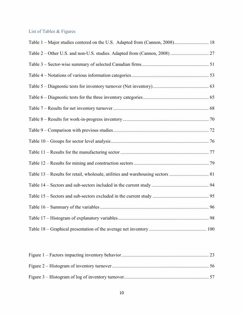
List of Tables & Figures

Table 1 – Major studies centered on the U.S. Adapted from (Cannon, 2008) ............................. 18

Table 2 – Other U.S. and non-U.S. studies. Adapted from (Cannon, 2008) ................................ 27

Table 3 – Sector-wise summary of selected Canadian firms ........................................................ 51

Table 4 – Notations of various information categories ................................................................. 53

Table 5 – Diagnostic tests for inventory turnover (Net inventory) ............................................... 63

Table 6 – Diagnostic tests for the three inventory categories ....................................................... 65

Table 7 – Results for net inventory turnover ................................................................................ 68

Table 8 – Results for work-in-progress inventory ........................................................................ 70

Table 9 – Comparison with previous studies ................................................................................ 72

Table 10 – Groups for sector level analysis .................................................................................. 76

Table 11 – Results for the manufacturing sector .......................................................................... 77

Table 12 – Results for mining and construction sectors ............................................................... 79

Table 13 – Results for retail, wholesale, utilities and warehousing sectors ................................. 81

Table 14 – Sectors and sub-sectors included in the current study ................................................ 94

Table 15 – Sectors and sub-sectors excluded in the current study ............................................... 95

Table 16 – Summary of the variables ........................................................................................... 96

Table 17 – Histogram of explanatory variables ............................................................................ 98

Table 18 – Graphical presentation of the average net inventory ................................................ 100

Figure 1 – Factors impacting inventory behavior ......................................................................... 23

Figure 2 – Histogram of inventory turnover ................................................................................. 56

Figure 3 – Histogram of log of inventory turnover ....................................................................... 57

11

List of Acronyms

TI – Inventory turnover for Net inventory

TIRM – Inventory turnover for Raw Materials

TIWIP – Inventory turnover for Work-in-progress

TIFG – Inventory turnover for Finished goods

CaIn – Capital intensity

SG – Sales Growth

Trevenue – Total revenue

IS – Inventory to sales ratio

OEM – Original Equipment Manufacturers

CM – Contract Manufacturers

JIT – Just-in-Time

PMI – Purchasing Managers Index

IA – Inventory to asset ratio

WRDS – Wharton Research Data Services

WIP – work-in-progress

12

1 Introduction

Inventory management is critical for managing firm’s assets in goods based industrial

sectors. Inventory holding costs represent about one third of the total of logistics costs (Johnston,

2014). Inventory costs represent the out-of-pocket costs for physically storing the product and

the lost investment opportunities due to the capital tied up in them (Cannon, 2008). Excess of

stock is seen as a cover up of various underlying operational problems (Cannon, 2008). So, the

conventional thinking suggests that it is pertinent to have inventories as minimum as possible to

free up capital, reduce costs or resolve operational difficulties.

The advent of Japanese companies in 1960-70s in the North American market had a huge

impact on the mindset of the companies with regards to inventory. The just-in-time and lean

philosophies were seen as a precursor of the decision to cut down the inventory levels. Western

companies were more oriented towards mass production in order to decrease the production and

the labor costs by achieving economies of scale. This strategy worked well in the time of

economic boom (Shingo, 1989). However, in the time of recession, this strategy appeared to

backfire and eat into the company’s capital in the form of excess inventory (Shingo and Dillon,

1989). At the same time, the Japanese companies, especially Toyota, still made profits in

difficult times (Shingo and Dillon, 1989). This made their western counterparts to take notice of

their strategy of lean and just-in-time which advocated the elimination of waste in terms of

inventory as well as unproductive work.

The western companies, impressed by this new philosophy of lean systems, started

adopting the principles of waste elimination. This led the companies to cut down on their

13

inventories. They tried to imitate the Toyota system of kanban and jidoka to emulate the success

of these companies. Some succeeded to a certain extent while others struggled with changing

their strategy (Thompson, 1997). However, one thing was clear – the companies were convinced

to reduce their inventories levels as much as possible. Along with just-in-time, trends like third-

party logistics, information technology, outsourcing and subcontracting have also encouraged

companies to undertake inventory reduction (Chen et al., 2007). However, there are also factors

such as higher customer service levels, an increase in the variety of product offerings and

uncertainty of demands that tend to push the companies towards higher inventory levels (Chen et

al., 2007).

Consequently, the question that arises is what happened to the inventory levels of

companies. Did they decline or increase with time or was there no trend at all? Numerous

academic studies have been done till date trying to answer the above question. A big majority of

the research is based on U.S. firms. Many of the studies centered on the U.S. manufacturing

sector do show a decline but there are some which state otherwise. Other sectors like wholesale

and retail show mixed results across studies. There are few papers examining firms other than

those in the U.S. Among these, the general trend is that the firms in larger economies tend to

show some decline in inventories. However, no such research has been found in the literature

which primarily focuses on Canadian companies. The purpose of this thesis is to perform an

empirical analysis of the inventory level of the companies in Canada over time. The investigation

takes place in two parts. First, the data on the net inventory level of publicly listed Canadian

firms are analyzed to determine whether there is an increasing or decreasing trend or no trend at

all. Also, along with net inventory, different types of inventory namely – raw materials, work-in-

progress and finished goods, are also examined for inventory time trends. In addition to the

14

above, this research also analyzes the impact of firm size, growth in sales, gross margin and

investment in fixed assets on net inventory for publicly listed Canadian companies.

The structure of the thesis is as follows. In the next section, various academic papers

related to the examination of inventory trends are discussed. It is followed by the third section

covering the proposition of hypotheses for the current study. The fourth section of methodology

comprises two sub-sections. The first sub-section provides a brief description of the database and

the definition of the variables. The second sub-section deals with the model specification and a

precise summary of the various models of time series panel data used for running the statistical

tests. The discussion of the results is presented in section five. The last section consists of the

conclusions, limitations and a brief note on possible future research.

15

2 Literature review

Inventory can be defined differently depending upon the field of study (Waller et al.,

2014). For financial accounting purposes, inventory is considered to be a part of the current

assets as it represents a tangible property that can be transformed into revenue (Waller et al.,

2014). From a supply chain perspective, inventory is seen as essential to balance demand and

supply (Waller et al., 2014). In short, inventory represents goods or stocks produced or held with

the purpose to sell or for maintenance.1

As per Waller et al. (2014), inventories can be classified based on the purpose of the

stock, based on the production stages and other criteria. The classification based on the

production stages is used in this thesis. As per this classification, there are three categories of

inventories: raw materials, work-in-progress and finished goods. Raw materials are the

inventories that have been stocked for utilization in the production process and do not have a

parent material (Waller et al., 2014). They are used as the initial inputs for the production

process, e.g. minerals, grains, etc.2 Work-in-progress inventories are those that are processed into

the final product (Waller et al., 2014). Any item in the inventory that is derived from a parent

raw material and is not in the final form or output of the production process can be considered as

work-in-progress inventory. 3

1 http://dictionary.cambridge.org/dictionary/english/inventory 2 http://www.referenceforbusiness.com/management/Int-Loc/Inventory-Types.html

3 http://www.referenceforbusiness.com/management/Int-Loc/Inventory-Types.html

16

Goods obtained at the end of the production or assembly and ready to be sold to the

customers are called finished goods (Waller et al., 2014). Net inventory can be described as a

summation of goods procured externally, goods produced internally as well as materials and

supplies purchased for manufacturing.4 Some authors also use the term total inventory for net

inventory. As per Rajagopalan et al. (2001), it is generally considered inappropriate to use

inventory in the terms of monetary value alone to examine inventory behavior over time. They

further state that the output of an industry varies over time and inventory varies with the output

of that industry. Hence, a decline in output could lead to a decline in inventory thus not giving a

clear picture of the inventory trends. Therefore, most studies reviewed in the succeeding part of

the literature review use some form of relative measures of inventory. However, few studies do

use absolute inventory levels. Jain et al. (2014) use average quarterly inventories and Amihud et

al. (1989) utilize average annual inventories as their dependent variable. Robb et al. (2012) also

use the year-end inventories of the firms as their dependent variable.

The relative inventory measures used in the studies analyzed as a part of the literature

review are inventory turnover, inventory ratios, inventory days, inventory to asset ratio, and

inventory to sales ratio. Inventory turnover (TI) is defined as the ratio of the cost of goods sold to

the total or net inventory measured in monetary value (Gaur et al., 2005). Some studies like

Rajagopalan et al. (2001), Cheng et al. (2012) and Boute et al. (2003) employ inventory ratios as

their dependent variable. Inventory ratio is defined as the ratio of the inventory to the value of

shipments (Rajagopalan et al., 2001). Inventory to sales ratio (IS) is defined as the ratio of the

total or net inventory to annual sales (Shah et al., 2007). Few studies like Mishra et al. (2013) 4 HEC online library – Osiris user guide https://proxy2.hec.ca:3090/version-2016628/Search.QuickSearch.serv?_CID=1&context=35TZCN8NR6T9HQ1

17

and Lieberman et al. (1999) use the inverse of inventory to sales ratio as their dependent

variable. The third measure, inventory days is defined as the product of the net inventory and

number of days in a year divided by the cost of goods sold (Chen et al., 2005). Inventory to

assets ratio is defined as the total or net inventory to total assets in a year (Chen et al., 2005). The

total assets in the above ratio could be substituted with fixed or current assets or capital

investment which all form subsets of the inventory to assets ratio (Blazenko et al., 2003).

Numerous academic research has been carried out to ascertain whether inventories have

actually decreased or not. The two main approaches taken by various researchers is either to

analyze the aggregate sector level behavior or to perform the same by utilizing firm level data. In

the first sub-section, the five major studies on this topic are analyzed in detail. Then, in the

second sub-section, studies inspecting the factors impacting inventory trends are reviewed. All

the papers covered in the two sub-sections are centered on the U.S. economy or U.S. firms. In the

third sub-section, studies examining the inventory trends of companies in non-U.S. economies,

including China, Germany, etc., are taken into consideration.

2.1 Five major studies – U.S.

The five most cited studies concerning the topic of this thesis are listed in Table 1. In this

table, we indicate the authors in the first column, the data source in the second column, time-

period of the respective study in the third column, dependent variable and sector in the last two

columns of the table. Many of the later studies take the work of these authors as a reference to

build their methodology and utilize several of the variables used in these studies.

18

Authors Data Timeline Dependent

Variable

Sector

Rajagopalan and

Malhotra (2001)

U.S. Census

Bureau – 20

sectors

1961 – 1994 Inventory Ratios Manufacturing

Gaur et al. (2005)

Financial reports

- 311 publicly

listed firms

1987 – 2000 Inventory

turnover

U.S. retail

Swamidass (2007) S&P Compustat

– 1200 firms

1981 – 1998 Total inventory

to sales

U.S

manufacturing

Chen et al. (2005)

WRDS

Compustat –

7433 firms

1981 – 2000 Inventory days,

Inventory to

asset ratios

U.S -

manufacturing

Chen et al. (2007) WRDS

Compustat –

1662 firms

1981 – 2004 Inventory days,

Inventory to

asset ratios

U.S – retail &

wholesale

Table 1 – Major studies centered on the U.S. Adapted from (Cannon, 2008)

Rajagopalan and Malhotra (2001) investigate 20 industries in the manufacturing sector

using data from the U.S. Census Bureau for the period 1961-1994. Making use of inventory

ratios and data for all the three types of inventory, i.e. raw materials, work-in-progress and

finished goods, they find that the total inventory measured in terms of inventory ratios declined

with time with a greater decrease in the pre-1980 period compared to post-1980. They also

conclude that among the various types of inventories, the raw materials and work-in-progress

inventory ratios showed a decline in the majority of the industries. However, the finished goods

19

inventory ratios did not show a specific trend due to mixed results. Work-in-progress showed the

sharpest decline among all the classifications of inventory. Similar results were found by Chen et

al. (2005) who use firm level data of public listed U.S. companies in the manufacturing sector

from WRDS (Wharton Research Data Services) compustat. They use inventory days which is

defined as the average number of days for the inventory to turn over and is computed through the

product of inventory and the number of days in a year divided by the cost of goods sold (Chen et

al. 2005). Using the interest rates, GDP growth, inflation rate and Purchasing Managers Index

(PMI) as explanatory variables, the results showed a decline in inventory days for total inventory

across the study period. Also, a larger decline was observed in work-in-progress inventory days

and a smaller but significant decline in raw materials inventory days. No trend was observed for

finished goods inventory. To counter check their results, Chen et al. (2005) perform the same

tests using inventory to asset ratio as a proxy for inventory. The decline in inventory to asset

ratio was found to be more drastic than for inventory days.

Relating raw materials inventory with interactions with suppliers, work-in-progress

inventory with internal operations and finished goods inventory with customer interaction, Chen

et al. (2005) suggest that the manufacturers have improved upon their efficiency in terms of

internal operations and communication and working with their suppliers. However, they attribute

the lack of decline in finished goods inventories to increasing product varieties and higher levels

of customer service expectations. These factors could have nullified the impact of JIT on

finished goods inventories.

Overall, work-in-progress inventories have shown the maximum improvement for the

majority of the firms included in their study. Using the same set of variables, Chen et al. (2007)

perform a similar analysis on 1662 publicly listed firms in the retail and wholesale sector of the

20

U.S. for the period from 1981 to 2004. The only difference here is that the authors only consider

total inventory for their test. The inventory days for the wholesale sector companies declined

from 73 days in 1981 to 49 days by 2004. This results in an average of 3% decline per year. The

retail sector companies had inventory days of 72.6 days in 2004; a mere 12-days decline from

1981.(Chen et al., 2007)

On detailed observation of the test results of Chen et al. (2007), it was found that the

inventory days increased in the initial years and remained unchanged until 1995. The decline

begins to appear post-1995. However, the overall period is trendless for the retail sector firms.

Similar results were observed for tests having inventory to asset ratios as the dependent variable.

Among the 21 sub-sectors in wholesale, except for two, all the sub-sectors show a decline in

inventory measured in terms of inventory to assets ratio, whereas most of the 14 sub-sectors in

retail did not show any decline. Chen et al. (2007) attribute the lack of decline in the retail sector

to the reasoning that the firms were more concerned with higher service levels and larger product

varieties.

Gaur et al. (2005) undertake another in-depth analysis of the U.S. retail sector. They

utilize inventory turnover as a proxy for inventory along with capital intensity, sales surprise and

gross margin as explanatory variables. The inventory turnover (TI) is defined as the ratio of the

cost of goods sold to the total inventory in monetary value (Gaur et al., 2005). Capital intensity is

described as a measure of investments in warehouses, IT, logistics and inventory management

systems and sales surprise is defined as a measure of the degree of difference between the actual

sales and the forecasts (Gaur et al., 2005). The regression results of Gaur et al. (2005) suggest

that the overall inventory turnover showed a downward trend over time implying that the relative

inventory levels have been increasing for the sample firms as a whole. But nearly 38% of the

21

firms show an increase in inventory turnover implying a decline in their relative inventory levels.

Also, the inventory turnover was negatively correlated with the gross margin and positively

correlated with the sales surprise and capital intensity. Gaur et al. (2005) contend that the overall

worsening of inventory trends may be partly attributed to the increased product varieties, shorter

life cycles of products and longer lead time for products due to global outsourcing.

In order to get a more in-depth view of inventory in manufacturing within the framework

of financial performance, Swamidass (2007) takes a unique approach. He argues that the reason

for the ambiguous results for inventory trends found in the literature, i.e. some studies showing a

decline in inventory and others proving the opposite, is because the firms within a given industry

are treated as a homogenous lot. Thus, he prefers to investigate the inventory behavior of the

firms distinguished by their financial performance. He takes a sample of 1,200 firms from the

S&P Compustat data and divide them into three groups of top performers, middle and bottom

performers on a financial basis. To establish a clear distinction between all the firms, they are

ranked on their financial performance and the average inventory of the top 10% firms are

compared with the middle 10% and the bottom 10% firms.

Performing a time series analysis of inventory to sales ratio against time with no other

control variables, the result of Swamidass (2007) showed no specific overall trend for the entire

data set. However, on taking a closer look at the result at each level, it is found that the top 10%

and middle 10% firms showed a downward trend or improvement in the inventory to sales ratio

whereas the bottom 10% showed an increase or worsening of this ratio. Also, for the period 1981

– 1990, the overall trend is negative but for the period from 1991 – 1998, the top 10% showed no

significant trend. The middle 10% showed a downward trend whereas the bottom 10% firms

showed an increase in the ratio (Swamidass, 2007). In addition to the above, his results suggested

22

that the gap between the top 10% firms and the bottom 10% firms tends to grow with time.

Though the study is interesting, doubt can be cast over the results as no control variables have

been taken into consideration, whereas other studies showed that the control variables can have

an impact. Also, the results obtained by comparing just the top and bottom 10% firms cannot be

generalized for the entire sector or industry. Nevertheless, it gives a different perspective for

looking at the inventory behavior.

Based on the five papers discussed above, it could be concluded that the U.S.

manufacturing sector showed a decline in inventories for both sector-level and firm-level

analysis. All the three papers on the manufacturing sector – Rajagopalan et al. (2001), Chen et al.

(2005) and Swamidass (2007) more or less agree with some sort of decline in inventories. This

decline is more profound in the period prior to 1990. Rajagopalan et al. (2001) performing a

sector level analysis and Chen et al. (2005) performing a firm level study, both indicate a decline

in raw materials and work-in-progress inventories and no trend for finished goods inventory.

Also, the work-in-progress category showed the highest improvement among all the categories

of inventory. The wholesale sector too has shown a substantial decline in Chen et al. (2007) but

the retail sector is trendless or showing signs of worsening of inventories in Chen et al. (2007)

and Gaur et al. (2005) respectively.

2.2 Factors impacting inventory trends

The above five papers focused on the inventory trend across time as the main subject of

analysis. However, many academicians prefer to focus their analysis on one specific aspect of

business like – globalization, investments in IT, implementation of JIT and lean systems and

many others and study their impact on the inventories. Below is a generic diagram (Figure 1) of

various factors impacting the firm inventory levels.

23

Figure 1 – Factors impacting inventory behavior. Adapted from De Leeuw et al. (2011)

Moving further, the seven factors mentioned in the Figure 1 and their impact on

inventories are analyzed in the studies listed in the Table 2 to get more insights on inventory

trends. The discussion of the literature in this section is organized around these seven factors.

Each of them will be discussed in a separate subsection. Table 2 contains a mix of studies from

U.S. and non-U.S. economies. In this table, we indicate the authors in the first column, the data

source in the second column, time- period of the respective study in the third column, dependent

variable and sector in the last two columns of the table.

Authors Data Timeline Dependent

Variable

Sector

Johnston (2014) S&P Compustat

– 126 firms


turnover,

Inventory to

Retail – U.S.

24

asset ratio

Cannon (2008) S & P Compustat

– 244 firms


turnover

Manufacturing –

U.S.

Cheng et al. (2012) U.S. Census

Bureau – 165

sectors

2003 – 2008 Inventory ratios Manufacturing –

U.S.

Blazenko et al.

(2003)

U.S. – publicly

listed firms; S&P

Compustat

1976 – 1995 Inventory to

invested capital

ratio

Across industry –

U.S.

Demeter and

Matyusz (2011)

IMSS 4 –

International

Manufacturing

strategy survey.

711 firms

February 2005

to march 2006

Inventory days Manufacturing –

23 countries

Demeter (2003)

IMSS 2 –

International

Manufacturing

strategy survey.

444 firms


turnover

Manufacturing –

23 countries

Huson and Nanda

(1995)

Questionnaire &

S&P Compustat

– 55 firms


turnover

Manufacturing –

U.S.

Vergin (1998) Fortune 500

(Compact

disclosure guide)

– 427 firms –


turnover

95%

manufacturing,

rest retail, mining

etc.

25

Han et al. (2008) Sector level –

U.S. Census

Bureau

2002 – 2005 Inventory days U.S.

manufacturing

Jain et al. (2014) U.S. Compustat

& U.S. customs

–

177 firms


investment

U.S. – retail &

Wholesale firms

Lieberman et al.

(1999)

Suppliers & part

manufacturers –

Surveys

1993 Sales/ average

inventory

U.S. & Canada

automobile

sector

Kros et al. (2006)

Research Insight

Database – 316

firms


turnover

Automobile,

electronics and

aeronautics –

U.S.

Amihud and

Mendelson (1989)

S&P Compustat

Database – 1,601

firms

1968 – 1986 Average

inventory and

inventory

variance

U.S.

Manufacturing

Irvine (2003) Sector level –

U.S. Dept. of

Commerce

Bureau of

Economic

analysis


sales ratio

U.S. –

Manufacturing,

retail, wholesale

De Leeuw et al.

(2011)

Interviews &

Surveys –

Inventory days U.S. -

Automobiles

26

dealers &

management –

119 interviews

Mishra et al.

(2013)

S&P Compustat,

CSRP – Centre

for Research in

Security Price,

Information

Week journal.

197 firms

2000 – 2009 Sales to

Inventory ratio

U.S. –

Manufacturing,

Retail, Mining,

wholesale,

Transportation,

construction etc.

Shah et al. (2007) Sector level data

– BEA from

Dept. of

Commerce

(U.S.)


sales ratio

U.S. –

Manufacturing,

retail, Wholesale

Dehning et al.

(2007)

S&P CompuStat

– 123 firms


turnover

U.S.

manufacturing

Boute et al. (2003)

National Bank of

Belgium – 15

sectors of

manufacturing

1979 – 2000 Inventory ratios Manufacturing,

Retail, wholesale

- Belgium

Shan et al. (2013) Wind financial

database – 1286

firms

2002 – 2009 Inventory/

operating cost

9 industries -

China

Robb et al. (2012)

ISI emerging

market database

1990 – 2008 Inventory to cost

of cost sold

Manufacturing -

China

27

– 294,914 firms

Kolias et al. (2011)

Financial reports

– 566 firms


turnover

Retail-Greece

Obermaier (2012) Sector level –

German Central

Bank

1971 – 2005 Inventory / sales Manufacturing,

Wholesale &

Retail - Germany

Lieberman et al.

(1999)

Financial reports

– 52 automobile

firms

1965 – 1991 Inventory/ sales Automobile

sector - Japan

Table 2 – Other U.S. and non-U.S. studies. Adapted from (Cannon, 2008)

2.2.1 Firm size

Johnston (2014) utilizes a similar set of variables as Gaur et al. (2005) along with the

firm size and net margin as additional explanatory variables. The results of Johnston (2014)

showed that the inventory turnover increased on average by 0.28% annually ignoring firm size.

However, by taking firm size into account, the inventory turnover showed a decrease from 1982

to 1994, implying an increase in the relative inventories and then a small increase in TI from

1998 to 2001 pointing towards a decline in the relative inventories. There is no long-term trend

for the selected retail firms. This result is in line with Chen et al. (2007) who find a decline only

around 1995. In contrast, Gaur et al. (2005) conclude an overall worsening of the inventory

levels with no exception in any of the years under study. However, Johnston’s results for

Inventory to assets ratio (IA) showed a continuous decline over the whole period of 30 years. He

28

prefers TI over IA as the impact on IA could be biased due the fact that IA could be improved by

decreasing the investments in inventories but increasing assets in the form of retail outlets,

distribution centers and transport equipments. Vergin (1998) takes a sample of 427 companies

from the list of the Fortune 500 companies and found that the inventory turnover improved for

eight consecutive years before a drop in 1995. Inventory turnover for firms making industrial

products increased, whereas it decreased for firms engaged in consumer goods. The results of

Cannon (2008) also showed a decline in the relative inventory level for a sample of 244

manufacturing firms with inventory turnover (IT) as the dependent variable and capital intensity,

firms’ employee base as proxy for the firm size and time as independent variables.

Thus, as seen above it can be noted that the firm size does have a significant impact on

the inventory. However, the results are somewhat contradictory and confusing. Johnston (2014)

points towards a worsening of the inventory trend in retail, whereas Vergin (1998), which

includes a sample of top performers across sectors and Cannon (2008) show signs of

improvement. First, it could be that the dependent variable for inventory or even the variables

used to estimate the firm size could be impacted by the choice of other explanatory variables

considered in these studies and behave differently under the influence of a different set of

independent variables.

2.2.2 Globalization

Some academicians argue that many of the original equipment manufacturers (OEMs)

source part or most of their products from contract manufacturers (CMs) which could result in a

redirection rather than a reduction of inventories (Han, Dresner & Windle, 2008). The OEMs

29

could be just pushing the entire excess inventories on their suppliers and contractors. Also,

contracting leads to longer lead times in turn resulting in larger safety stocks. Cheng et al. (2012)

favor sector-level data rather than individual firm-level data given that in most cases both OEMs

and contract manufacturers are in the same sector.

As per Cheng et al. (2012), outsourcing can have two opposite impacts. Globalization can

lead to cheaper raw materials and lower production costs. However, an increase in the distance

generally results in longer lead times and a higher risk due to natural calamities necessitating

higher safety stocks. Their analysis shows that outsourcing leads to a reduction of raw materials

and finished goods inventories but not for work-in-progress inventory. They conclude that

contract manufacturers can pool production across many OEMs, thus achieving economies of

scale by inventory pooling which in turn helps in reducing safety stock. Han et al. (2008) try to

find out the impact of globalization on inventory in the form of import and export ratios for

individual sectors. The import ratio is defined as the ratio of imported raw materials to the total

purchases per sector (Han et al., 2008). The export ratio is defined as the ratio of the exported

finished goods to the total sales within the sector (Han et al., 2008).

The results of Han et al. (2008) show that the inventory costs are positively correlated

with the import and export ratio. An increase of 10% in imports leads to an increase of 2.16 days

of inventory. Similarly, increasing exports by 10% results in augmenting the inventory days by

2.05 days. While Han et al. (2008) concentrate on the impact of global operations in terms of

imports and exports on inventory, Jain et al. (2014) investigate the impact of global sourcing in

terms of imports and supplier diversification on inventory. They deduce a positive relationship

between global sourcing and inventory investment and a negative relationship between supplier

dispersion and inventory investment. A 10% increase in global sourcing would lead to an 8.8%

30

higher investment in inventories for the sample firms despite reduced costs of inventory.

However, a larger dispersion of the supplier base reduces the dependency and uncertainty for the

firms resulting in lower inventory investments.

Cheng et al. (2012) and Jain et al. (2014) support that contract manufacturing and higher

supplier diversification cause reduction in inventories. However, Han et al. (2008) contradict it

by showing that a higher level of globalization results in higher inventory investments.

2.2.3 JIT & lean systems

There is another set of academicians who make a comparison between lean and non-lean

companies or take a sample of self-proclaimed JIT firms to show the impact of the principle of

waste elimination on inventories. Demeter and Matyusz (2011) use the 4th edition of the IMSS

(International Manufacturing Strategy Survey) to compare between 171 lean and 84 non-lean

companies from across 23 countries, including 25 from Canada. The findings of Demeter and

Matyusz (2011) suggest that lean companies showed significantly smaller inventory days across

various types of inventory compared to non-lean ones. However, within lean firms too, there was

a significant difference in the impact on inventories based on the production systems and order

type. The choices of production system, i.e., whether modular or dedicated lines, impacted work-

in-progress inventory the most. The higher the ratio of dedicated lines, the lower is the work-in-

progress inventory. Secondly, the order policy has a profound impact on the inventory of raw

materials and finished goods. Demeter et al. (2011) show that make-to-order had a strong

positive correlation to raw materials inventory while assemble-to-order is negatively associated

with it. On the other hand, make-to-stock results in higher inventory days for finished goods

inventory.

31

Demeter, using the same strategy as above, divides a list of 444 companies from IMSS –

2 survey into firms with and without manufacturing strategy and finds no significant correlation

between inventory turnover and manufacturing strategy (Demeter, 2003). Thus, a conflicting

result is obtained from two surveys. IMSS-4 was compiled in a more recent period and is

considered to have more authentic data compared to IMSS-2 as the latter was conducted at the

initial stages. So there are chances of recording inappropriate responses in earlier version. Also,

for IMSS-4, Demeter does filter out a large number of small and medium-sized companies and

includes only large scale firms for analysis. Demeter argues that the reason to exclude small and

medium firms is that most of them do not have the resources or capital to invest in lean

production for effective inventory management.

Huson and Nanda (1995) take a sample of 55 U.S. manufacturing firms based on

newspaper articles related to JIT implementation and mailed them a questionnaire to obtain the

details including commencement date of JIT implementation. They obtain the information on

inventories, number of employees, unit margins and earnings per sales from the financial

statements of these firms published in S&P Compustat. The results suggested an average

increase of 24% in the inventory turnover in the period after the JIT implementation. Also, there

was a decrease in employee per sales dollar of approximately 34% by the end of the study period

pointing towards improved labor productivity. The findings of Fullerton et al. (2001) indicate

that firms had a substantial reduction in inventory levels post implementation of JIT. A greater

reduction was found in work-in-progress and raw material inventory while there was

substantially less decline in finished goods inventory. This is in line with the findings of

Rajagopalan et al. (2001) and Chen et al. (2005). Almost all the papers focusing on JIT

implementation like Fullerton et al. (2001), Huson et al. (1995) and Demeter et al. (2011)

32

unanimously agree that the implementation of just-in-time principles does lead to a decline in

inventory levels.

2.2.4 Industry

Some researchers prefer to select a particular industry/s like automobile or aeronautics

where the impact of JIT (just-in-time) is considered to be profound instead of the whole

manufacturing sector for their analysis. Based on the survey of tier-1 suppliers to assemblers in

the U.S. and Canada automobile industry, Lieberman et al. (1999) find a negative correlation for

work force training and customer communication with inventory levels. Plants which had their

workforce trained in a formalized improvement process had almost half the level of inventory

compared to those plants where there was no emphasis on process improvement at the

production lines. Another significant outcome was that the plants which had closer and more

frequent communication with customers had lower inventories than those who did not

(Lieberman et al., 1999).

There was no significant difference in the inventory levels of Japanese-owned plants and

plants owned by the U.S.-based automobile companies. In fact, the regression results of

Lieberman et al. (1999) showed that the Japanese plants had higher inventories in terms of

finished goods and work-in-progress compared to the average inventory of their U.S. and

Canadian counterparts. The authors suggest that the Japanese firms may have decided to have

larger inventories to adapt to the conditions in North America with lower real estate prices and

longer transport distances compared to Japan.

Kros et al. (2006) focus on the inventory of the supplier firms in the automobile,

aeronautics and electronics industry. Their analysis showed that for the electronics industry, the

33

inventory ratios for raw materials and work-in-progress improved over the period but the

finished goods and total inventory ratios worsened. For aeronautics, there was not much change

in any of the inventory ratios. Surprisingly, the suppliers in the automobile industry as well did

not show any significant changes in the inventory ratios. Kros et al. (2006) also make a

comparison between Original Equipment Manufacturers (OEM) and their suppliers for all the

three industries. They do not find any similarities in terms of trends in the inventory ratios of

OEMs and their suppliers for all the three industries. The reason as per Kros et al. (2006) could

be that the inventories were not eliminated but rather moved upstream from OEMs to their

suppliers. Another point to be noted is that this study was done in the latter part of the 1990s,

long after the concept of JIT was widely accepted. It might be a possible explanation that these

firms and their suppliers, especially in the automobile segment, may have implemented JIT long

ago and by the time of the commencement of this study the elimination of excess inventory had

already reached saturation. Hence, no trend is seen in the inventory ratios here.

De Leeuw et al. (2011) on the other hand, focus on the inventories downstream at the

dealers and retailers side belonging to the U.S. automobile industry. The reason for this is that

the decision making is more localized in the industries highly dependent on dealers, retailers and

distributors. Their focus was mainly on dealers of passenger vehicles in five major regions of the

U.S. The authors find a negative correlation between the sales objective of dealers and the sales

through fulfillment of customer orders directly from the factory. Also, the inventory days at the

firm level is negatively correlated to the outlets’ sales objective. The main logic behind this as

per De Leeuw et al. (2011) is that more sales require more inventories and conversely more

inventory would lead to a higher amount of sales. No statistical connection was found between

the firm level inventory and the dealers’ level inventory. The reason based on the interviews was

34

that the firms allocated quantities and models through a well-negotiated process in which the

dealers had to take a large number of cars of the models that did not sell well to get larger stocks

of the popular or bestseller models. Hence, the firms use their power to get rid of the inventory in

their factory by restricting the allocation of high demand models to dealers. This, coupled with

the customer unwillingness to wait for orders pushes the dealers to stock up large piles of

inventory in order to be able to sell from their own stock (De Leeuw et al., 2011).

Comparing the results of the supplier side and retailer or dealer side inventories from the

above studies, it could be noted that De Leeuw et al. (2011) and Kros et al. (2006) show that the

suppliers and dealers or retailers in the automobile sector have been faced with a deterioration of

their inventory trends, whereas Lieberman et al. (1999) show a marked improvement in the

inventory of manufacturers and only tier-1 suppliers who focus on the employee productivity and

strong customer communication in the automobile industry. This disproves the notion that

retailers, suppliers and manufacturers are a homogenous lot and confirms that the retailers and

suppliers do not show the same inventory trends as the manufacturers. This may also point to the

fact that manufacturers try to push the inventory downstream and the dealers try to sell it off at

discount prices to clear them.

2.2.5 IT investments

A few researchers try to analyze the impact of IT investments on inventory levels (e.g.

Shah et al. (2007), Mishra et al. (2013) and Dehning et al. (2007)). Analyzing sector level data

for the U.S., Shah et al. (2007) show that an increase in IT investments has a negative correlation

with the inventory levels for the manufacturing and the retail sectors but has no impact on the

inventory levels of the wholesale sector. On the whole, the manufacturing sector showed a

35

continuous decline, whereas the inventory levels showed a growth in the retail and the wholesale

sector. Mishra et al. (2013), on the other hand, arrive at the same conclusion utilizing firm level

data for the U.S. They too affirm the positive impact of investment in Information Technologies

on inventory performance.

Shah et al. (2007) also state that IT investments have a positive impact on the financial

performance indirectly mediated by an improvement in inventory levels but no direct correlation.

In contrast, Mishra et al. (2013) show a direct impact of IT on financial performance of firms and

a partial impact mediated by inventory performance. Dehning et al. (2007) also find the positive

impact of IT-based supply chain management systems on the inventory level of manufacturing

firms. All the three papers agree on a negative correlation between information technology and

the relative inventories.

2.2.6 Competition, profit margin & industry concentration

Blazenko and Vandezande (2003) state that the characteristics of firms’ demand and

marketing environment play a crucial role in determining inventory levels. Their findings

suggest that higher profit margins have a positive impact and industry concentration has a

negative impact on inventory levels. Higher profit margins induce firms to have larger

inventories to avoid stock outs. Higher competition implies lower market power and hence less

industry concentration. In presence of competition, firms prefer to have larger inventories to

avoid stock outs as its impact on the revenue over the long term is greater due to customers’

switching to other alternatives.

Amihud and Mendelson (1989) tried to ascertain the impact of the market power of firms

on their inventory. They find a positive relationship between market power and inventories of the

36

firm. In case of higher market power, the firms tend to have larger inventories to absorb the

shocks from demand and supply fluctuations. This is in contrast to the findings of Blazenko et al.

(2003) who state that lower industry concentration leads to larger inventories.

2.2.7 Unique response variable – Fixed weight Inventory to sales ratio

Some academicians like Irvine use a more unconventional method of defining their

response variable for the inventory. Irvine (2003) argues that many of the previous studies do not

reflect the reality of the inventory because of the measures they use. He suggests using fixed

weight inventory to sales ratios (FWIS) instead of aggregate inventory to sales ratio (AIS). The

main difference in the above two measures is that in the fixed weight IS, ratio an aggregation

weight is associated with each sub-sector’s inventory in proportion to its sales. In the aggregate

IS, the inventories of all the sub-sectors are added and taken into consideration with the

summation of sales across all the sub-sectors.

The aggregate inventory to sales ratio of the U.S. Department of Commerce Bureau of

Economic Analysis (BEA) shows that the IS ratio for the retail and the wholesale sectors is

trending upwards whereas for the manufacturing sector it showed no trend. But using the fixed

weight IS ratio, Irvine (2003) concludes that all the three sectors showed a downward trend in

the relative inventory levels measured in terms of fixed weight IS. The most significant finding

of this research is that most of the downward trend in all the three sectors is in the sub-sectors

selling durable goods, whereas those selling non-durable goods show an upward trend. Overall,

the sales mix has drifted towards durable goods across sub-sectors resulting in an overall

downward trend.

37

Fitting time trends into the fixed weight aggregate IS ratio, Irvine (2005) tries to find the

exact year of the break in the inventory sales ratio trends. The decrease in the inventory to sales

ratio for the total manufacturing sector started in 1983, for wholesale in 1985 and for retail in

1990.

2.2.8 Inventory trend and financial impact

There are also several empirical studies which focus on inventory behavior and financial

performance. Chen et al. (2005) find that the inventory level did not have an immediate impact

on the financial performance of the firms but had a long-term impact, i.e. in the long run, firms

with abnormally high inventory levels had very poor long-term stock returns. Companies with a

medium level of inventory had the best returns whereas companies with the least inventory level

had ordinary returns. This was true for the firms in the U.S. manufacturing and wholesale sector

but the U.S. retail sector showed no clear relation between the financial performance and

inventory levels (Chen et al., 2005). Huson and Nanda (1995) demonstrate that a JIT adoption

has a positive correlation with inventory as well as financial performance and the earning per

shares also improved.

Shah et al. (2007) and Dehning et al. (2007) agree that inventory levels mediate the

positive impact of IT investment upon the financial performance of the firms. Mishra et al.

(2013) find a direct positive impact of inventory and IT investments on financial performance.

However, Cannon (2008) did not to find any correlation between inventory and financial

performance. He finds the correlation to be positive for some firm and negative for others; but

overall, there was no impact. Fullerton et al. (2003) indicate that the firms with JIT

implementation have better financial rewards and improvement in the financial performance. A

38

detailed analysis on the financial impact of inventory performance will not be discussed here as

it is not a part of the research question of this thesis.

2.2.9 Discussion

Based on the above literature review, it could be noted that firm size, level of IT

investments, supplier and dealer relationship, globalization, competition, ordering type etc. have

a significant impact on inventories. But whether the inventories declined or increased is difficult

to say. Conflicting results are obtained on inventory trends under the influence of firm size while

comparing the studies of Johnston (2014) Vergin (1998) and Cannon (2008). Also, when it

comes to suppliers, Cheng et al. (2012) and Jain et al. (2014) show a decline in inventories due to

supplier diversification and contract manufacturing but Kros et al. (2006) show no improvement

in inventories of suppliers and Han et al. (2008) point towards a deterioration of inventories for

manufacturers having global operations. In contrast, Lieberman et al. (1999) show an

improvement in inventories of Tier 1 suppliers of the U.S. automobile industry. De Leeuw et al.

(2011) point towards a deterioration of the inventory trends at the retailers’ side of the supply

chain. Blazenko et al. (2003) suggest that firms with a lower industry concentration and market

power tend to have larger inventories whereas Amihud et al. (1989) indicate that firms with

larger market power maintain larger stocks.

However, there is some consensus among the studies concentrated in studying the

impact of JIT and IT investments on inventory behavior. All the studies, Demeter et al. (2011)

Huson et al. (1995) and Fullerton et al. (2001), agree that a JIT implementation results in lower

inventories. Similarly, the results of Shah & Shin (2007), Mishra et al. (2013) and Dehning et al.

39

(2007) all concur or acknowledge the negative correlation between IT and IT-based investments

with the inventory behavior.

When it comes to the sector level analysis, many of the studies focusing on the U.S.

manufacturers show a decline in their inventories. However, the results are conflicting for the

U.S. wholesale sector. Chen et al. (2007) and Irvine (2003) find an improvement in the

wholesale sector whereas Shah et al. (2007) point to a deterioration of the inventory trend for the

same. For the U.S. retail sector, none of the papers studied so far except one, show any

improvement in these inventory levels. Chen et al. (2007) and Johnston (2014) point towards no

significant change in inventories of retail firms. Shah et al. (2007) and Gaur et al. (2005) find an

increase in inventories of the U.S. retail firms. Only Irvine (2003) points towards a decline in

them. Additionally, better customer communication and work force training tend to help

companies in streamlining their inventory management (Lieberman et al., 1999).

Overall, it is difficult to say what happened or is happening to the inventories. All the

above studies suggest or indicate mixed or conflicting results on comparison and it is difficult to

make exact conclusions about the inventory trends based on them.

2.3 Non-U.S. studies and discussion

Until now, most of the analyses have been performed using data from U.S. firms or U.S.

sectors. It is difficult to conclude a single result from the reviewed studies except that at an

aggregate level, the manufacturing sector of the U.S. did show a decline in inventories at least

until the 1980s. However, the other question is whether the results of the U.S.-based studies can

be generalized to firms in other countries. To ascertain how the inventories in other economies

40

behave, studies pertaining to significant economies outside North America like China, Germany

and others are analyzed in the further part of the literature review.

2.3.1 Non-U.S. studies

Boute et al. (2003) replicate the work of Rajagopalan et al. (2001) for Belgian firms in

the manufacturing, retail and wholesale industry with time and sector growth as explanatory

variables. The raw material inventory ratios showed significant decrease for eight sub-sectors,

work-in-progress inventory ratios declined in six sub-sectors but finished goods inventory ratios

showed a decrease for only in four sub-sectors. Thus, overall the authors conclude that there is a

decrease in inventory levels of manufacturing firms, but it is statistically smaller compared to

U.S. manufacturing firms. Further, Boute et al. (2003) analyze the finished goods inventory ratio

for the wholesale and retail companies of Belgium. They observe a significant decrease in the

finished goods inventory level for retail firms but no significant decrease for firms in the

wholesale sector for Belgium. This contrasts with Chen et al. (2005) who find a decrease in the

inventories of U.S. wholesale firms but no trend for U.S. retail firms.

Shan et al. (2013) examine firms listed on the Chinese stock market and find a

statistically significant negative relationship between inventory and time. The relative inventory

levels measured in terms of inventory turnover dropped at a rate of about 1.5 % on average

annually. On the other hand, Robb et al. (2012) analyzing Chinese manufacturing firms also

conclude a decrease in the inventories across firms belonging to most sub-sectors in

manufacturing except those in the tobacco industry. They also examine the link between

inventories and the GDP per capita at a regional level within China and suggest a U-shaped

41

correlation. This signifies that Chinese regions or provinces with larger and lower GDP per

capita had higher inventories.

Kolias et al. (2011) replicate the methodology used by Gaur et al. (2005) for Greek retail

firms. They observe a decline in inventory turnover of about 3.4 % in a year signifying a

deterioration of inventory levels in retail firms. Also, inventory turnover was negatively

correlated to gross margins and positively correlated to sales surprise and capital intensity.

Dividing the Greek retail sector into two, i.e. regions with increasing sales and regions

with decreasing sales, Kolias et al. (2011) find that regions with declining sales showed larger

changes in the same direction in inventory turnover compared to firms in regions with increasing

sales. The reason they conclude for this behavior is that decreasing sales impact cash flows

negatively which in turn render firms unable to take advantage of quantity discounts and results

into increasing the operating costs which leads to a decline of the inventory turnover.

Utilizing inventory to sales ratio (IS) for the manufacturing, retail and wholesale sectors

for Germany, Obermaier (2012) finds a decrease in the IS ratio for raw materials and finished

goods while the IS ratio increased for work-in-progress inventory. This is in contrast to

Rajagopalan et al. (2001) where raw materials and work-in-progress inventory declined for U.S.

firms and also for Belgian firms in Boute et al. (2003). The overall total inventory declined for

all the sectors. Among the sectors, the manufacturing sector showed a larger decline during the

pre-1988 period whereas during the post 1988, the wholesale and retail sectors showed the

greatest decline in their respective total inventories in the sample of firms from Germany

(Obermaier, 2012).

42

Generally, the work-in-progress inventory is believed to be impacted most by the JIT

implementation but here we find a contrasting result (Obermaier, 2012). He attributes the reason

for this to the possible shift from a make-to-stock to a make-to-order approach among the

German firms or to the higher bargaining power of upstream companies compared to the rest in a

supply chain. In contrast to Obermaier (2012), Lieberman et al. (1999) show a decline in work-

in-progress inventory of 52 Japanese automobiles companies and their suppliers. The main aim is

to examine the impact of a JIT implementation in terms of work-in-progress inventory and labor

productivity. Lieberman et al. (1999) explain that inventory presence on the shop floor prevents

the discovery of problems on the shop floor. Reduction in work-in-progress inventory exposes

defects in the manufacturing process which induces the managers to eliminate the source of

process disruption. The results of Lieberman et al. (1999) show that most of the companies cut

their WIP/sales ratio by more than 50% from the late 1960s to the early 1980s. On the whole,

between 1970 and 1980, labor productivity grew on average by 9% annually. They also find a

negative correlation between labor productivity and IS ratio. A reduction of about 10% in IS

ratio resulted in approximately 1% improvement in labor productivity.

2.3.2 Discussion & Conclusion

Overall, except for Greece, results from all the other non-U.S. economies tend to show a

decline in total or at least in one of the inventory types. The decline for the firms in Belgium is

small, whereas the decline for China, the U.S., Japan and Germany is relatively large. The couple

of cross-country studies (Demeter, 2003) and (Demeter & Matyusz, 2011), do not give a clear

picture on the trends. From the above, it can be stated that the declining trend is seen in larger

economies whereas the trend is not that prominent in small ones. However, the duration of the

study is also something that cannot be ignored. For Greece, the study period is quite recent and

43

very small compared to the study period for the other economies. Maybe if the data was obtained

for an earlier period and for a larger duration, the results might have been different.

A decline in work-in-progress inventories is observed in studies concerning U.S., Belgian

and Japanese firms in Rajagopalan et al. (2001), Boute et al. (2003) and Lieberman et al. (1999)

while German firms show an increase in them (Obermaier (2012)). Only German firms show a

marked decline in finished goods inventory (Obermaier (2012)), whereas there is no trend or a

deterioration of finished goods inventory levels for the firms in other countries (Rajagopalan et

al., (2001); Boute et al., (2003); Lieberman et al., (1999)). The raw material inventory shows a

decline across Belgian, U.S. and German firms in their respective studies. So far, the results are

far from pointing to any particular direction when comparing sectors and inventory categories

across countries. Overall, one thing seems more certain that in general, manufacturing firms have

shown some decline in most studies for the U.S. and outside the U.S. as well.

Demeter et al. (2011) and Demeter (2003) are the only studies that take into consideration

a few firms from Canada. But their results are quite generic in nature and nothing can be deduced

in particular for Canada. Also, the number of firms is not sufficient to be representative of the

Canadian economy. Thus, after all the deliberation on the behavior of inventories across the

academic papers, it is still difficult to say with certainty what happened to the inventories.

Moreover, no paper specific to Canada has been found in the literature. The purpose of this thesis

is to try to fill this gap and to conduct a study that analyzes the inventory trends of Canadian

companies.

44

3 Research Objective and hypotheses

3.1 Research Objective

The objective of this thesis is to examine the evolution of net inventories as well as

various inventory categories for publicly listed Canadian firms. The inventory behavior is

examined over a period of 30 years from 1987 to 2016 to ascertain whether there is a decline or

growth in the inventory levels and compare the results with the studies discussed in the literature

review. Also, an attempt has been made to find a correlation between net inventory and various

firm level factors like company size, gross margin, investment in fixed assets and sales growth,

and to study their impact on the net inventory of the Canadian firms. Based on the analysis done

in the literature review, a detailed discussion of the hypotheses for the current study is provided

in the next sub-section.

3.2 Hypotheses

In this sub-section, five hypotheses will be proposed for this research. As discussed

previously in the introduction, the inventory is seen as lost investment opportunities due to the

capital tied up in them. Also, excess inventory is seen as a cover up of various operational

problems (Cannon, 2008). This coupled with the advent of Japanese firms in the 1970s, the

popularization of the just-in-time and lean philosophies in North America during the 1980s

would have led the domestic companies in Canada and the U.S. to try to minimize their

inventories as much as possible (Huson and Nanda, 1995). Additionally, various innovations in

the field of information technology like MRP, quick response, ERP, etc., would further augment

the effort to reduce inventories in order to achieve optimum operational efficiency (Rajagopalan

and Malhotra, 2001). Based on the above observations, the two parts of the first hypothesis for

45

net inventory and the three inventory classifications namely – raw materials, work-in-progress

and finished goods are stated as below.

Hypothesis 1-a:

Inventory turnover for net inventory of the Canadian companies is positively correlated

with time.

Hypothesis 1-b:

Similarly, inventory turnover for the raw materials, finished goods and work-in-progress

inventory of the Canadian companies is positively correlated with time.

A positive correlation between inventory turnover and time indicates that the ratios are

increasing with time implying relative inventories are showing a declining trend with time. This

is because inventory is inversely proportional to the inventory turnover. Here, a point to be noted

is that the inventory categories – raw materials, finished goods and work-in-progress inventory

are examined only for the time trends. The subsequent hypotheses with respect to the other

explanatory variables are examined for net inventory only.

Based on the surveys conducted among the retail firms in their study, Gaur et al. (2005)

suggest that the managers have to make a trade-off between gross margin and inventory turns.

Further, they infer that goods with a higher margin have lower turns compared to the low-margin

goods. Additionally, they explain a negative correlation between gross margin and inventory

turnover directly through the factors such as product service level and indirectly through product

price, product variety and its life cycle length. Shan et al. (2013) also suggest a positive relation

46

between gross margin and inventory on the premise of the stochastic inventory models. Based on

the above, the second hypothesis is as below:

Hypothesis 2:

Inventory turnover for net inventory of the Canadian companies is negatively correlated

with gross margin.

Capital intensity is defined as investments in fixed assets of a firm (Gaur et al., 2005).

Gaur et al. (2005) suggest that investment in fixed assets like warehouses, IT systems, etc., could

lead to a reduction of lead times and safety stocks for the retailers. Also, they further state that

the investment in fixed assets provides retailers more flexibility in dealing with uncertainty

related to shipment of inventories across the stores. A decline in inventory in turn results in

higher inventory turns. This leads to the third hypothesis.

Hypothesis 3:


with capital intensity.

Rumyantsev & Netessine (2007) state that the larger the firm, the better will be its ability

to pool demand from various assets like stores and warehouses resulting in lower inventory. In

short, a larger size of the firm helps it in achieving economies of scale in handling inventory.

They base their argument on the insights from stochastic models. Johnston (2014) agrees with

the above and proposes a hypothesis along similar lines of Rumyantsev et al. (2007). Shan et al.

(2013) also prove the negative correlation between firm size and inventories. Based on the above

research studies, the proposition for the fourth hypothesis is as below.

47

Hypothesis 4:


with firm size.

In their analysis, Rumyantsev et al. (2007) find a negative correlation of inventory with

sales growth for U.S. firms. Shan et al. (2013) also find a significant negative relation between

the two variables for Chinese firms. Here, the purpose of the current study is to examine the

relation between inventory and sales growth for the Canadian firms. The fifth hypothesis is as

below.

Hypothesis 5:


with sales growth.

A point to be noted here is that in case of raw materials, finished goods and work-in-

progress inventory, the focus is to investigate their respective time trends for the Canadian

companies. Their individual correlation with each of the explanatory variables will not be studied

in the current study. The reason is that the published studies analyzing these variables do so only

for net or total inventory. But none of them specifically investigates the correlation of these

variables with the three inventory categories. The purpose of the current study is to replicate the

methodology of some of the previous studies partly or completely as far as possible for the

Canadian firms rather than propose a new proposition based on theoretical models and test them.

48

4 Methodology

4.1 Database and variables

4.1.1 Database

The database for this research is obtained from the Osiris database. It consists of 53,060

listed companies from over 130 countries around the world as of July 2016. The Osiris database

is sourced from the following information providers – World’Vest Base, Reuters/Multex, Edgar

Online, Fitch Ratings Bank Data, Fitch Ratings Insurance Company, Korea information service

and Bureau van Dijk. The employees of these organizations and data analysts appointed by them

are fully trained in the task of data collections with a well-defined set of procedures and

numerous automated and manual error checks are in place to get the most accurate data. Also,

independent audits of listed firms and verification and authentication of the provided data are

done on a timely basis to ensure the accuracy of data. All the data are rigorously checked before

being submitted to Osiris.5

4.1.2 Selection criteria and firm characteristics

For the research purpose, the annual balance sheet and income statement data of a total of

2,523 publicly listed Canadian companies were accessed from the Osiris database from 1987 to

2016. The companies were selected based on the two-digit NAICS 2012 industry classification.

These 2,523 Canadian firms belong to ten sectors of the NAICS 2012 classification. These ten

5 HEC online library – Osiris user guide https://proxy2.hec.ca:3090/version-2016628/Search.QuickSearch.serv?_CID=1&context=35TZCN8NR6T9HQ1

49

sectors are – agriculture, forestry, fishing and hunting; construction; manufacturing; mining,

quarrying, oil and gas exploration; retail trade; transportation and warehousing; health care and

social assistance; accommodation and food services; utilities; wholesale.

Only those sectors where inventory plays a key role in the operations of firms were

selected. Sectors where inventory was insignificant like finance and insurance; real estate;

information; administrative, support and waste management; educational services; public

administration and arts; management of companies and enterprises; professional, scientific, and

technical services; entertainment and recreation were excluded. The complete list of sub-sectors

within each of the sectors included and excluded in the current study is provided in the Table 14

and Table 15 of the appendix. From the annual balance sheet and income statement data,

information with regards to net inventory, inventory related to raw materials, work-in-progress

and finished goods, total sales, revenues, cost of goods sold, gross margin, total assets and total

net fixed assets were extracted. The gross margin is expressed in percentage and all the other

information categories are expressed in thousand Canadian dollars. The above information

categories are also available on a quarterly basis, but the quarterly data is not available beyond

2008. Hence, the annual data of the firms was utilized for the empirical analysis.

Many of the firms had several missing values for many variables under the study and for

several years across the selected timeline of 30 years (1987 – 2016). To overcome the problem of

missing values, a second criterion for the selection of companies was applied based on Gaur et

al. (2005). They selected only the firms that had at least five years of continuous data for their

variables within the time duration of 14 years (1987 – 2000). On a similar basis, it was decided

that only those companies which had at least 10 years of continuous data for net inventory during

the studied period from 1987 to 2016, were taken into consideration. Firstly, since net inventory

50

data is used in defining the dependent variable, it is utilized as a criterion for the selection of

companies for testing. Without the inventory data, the rest of the information about the

individual companies is of little use. Secondly, since the studied period for this thesis is about 30

years, which is almost double the length compared to the one chosen by Gaur et al. (2005), it was

decided to have a longer period of 10 consecutive years for the selection criterion. This was done

in order to discard the companies that have too few observations to perform a time series

analysis.

After deleting the companies based on the above criterion, a total of 420 firms were left

for the purpose of analysis. Table 3 provides the information about the total number of firms in

each sector and their share of the total selected firms.

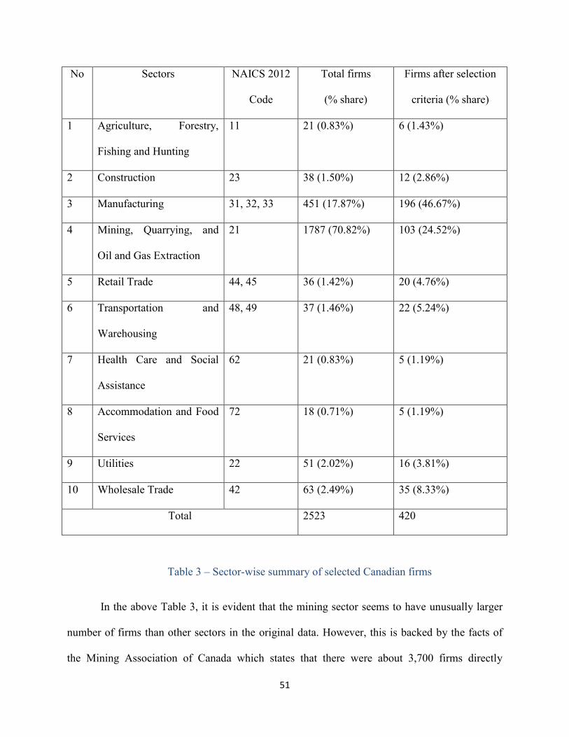
51

No Sectors NAICS 2012

Code

Total firms

(% share)

Firms after selection

criteria (% share)

1 Agriculture, Forestry,

Fishing and Hunting

11 21 (0.83%) 6 (1.43%)

2 Construction 23 38 (1.50%) 12 (2.86%)

3 Manufacturing 31, 32, 33 451 (17.87%) 196 (46.67%)

4 Mining, Quarrying, and

Oil and Gas Extraction

21 1787 (70.82%) 103 (24.52%)

5 Retail Trade 44, 45 36 (1.42%) 20 (4.76%)

6 Transportation and

Warehousing

48, 49 37 (1.46%) 22 (5.24%)

7 Health Care and Social

Assistance

62 21 (0.83%) 5 (1.19%)

8 Accommodation and Food

Services

72 18 (0.71%) 5 (1.19%)

9 Utilities 22 51 (2.02%) 16 (3.81%)

10 Wholesale Trade 42 63 (2.49%) 35 (8.33%)

Total 2523 420

Table 3 – Sector-wise summary of selected Canadian firms

In the above Table 3, it is evident that the mining sector seems to have unusually larger

number of firms than other sectors in the original data. However, this is backed by the facts of

the Mining Association of Canada which states that there were about 3,700 firms directly

52

involved or supporting mining operations in Canada as of 2014.6 However, the total share of

mining firms selected for the study is much lower compared with their share in the total firms.

This is due to the fact that a big majority of the mining firms do not have the required data in

their balance sheets and income statements. On the other hand, sectors like manufacturing,

wholesale, retail and warehousing have required data for around half of the total firms available

in each of these sectors. Hence, their share of firms selected for the study is higher. Due to the

lack of availability of required data in certain sectors, we recognize that this might lead to a non-

selection bias in our analysis. This is a limitation of the current study.

4.1.3 Variables

The various information categories stated in the previous sub-section are given notations

as shown in the Table 4.

Sr. No Information category Notation

1 Net stated inventory NI

2 Raw materials inventory RM

3 Finished goods inventory FG

4 Work-in-progress inventory WIP

5 Cost of goods sold COGS

6 Total net fixed assets TNFA

7 Total assets TA

8 Sales Sales

9 Gross margin GrossMargin

6 http://mining.ca/resources/mining-facts

53

10 Total revenues Trevenue

11 Companies ID

12 Study period (1987 – 2016) Year

Table 4 – Notations of various information categories

Here, each Canadian company whose data is utilized in the regression is given a unique

identification number denoted by ID. The above notations are used to describe our dependent

variables and explanatory variables. ID is the panel variable. The panel variable here represents

the entities under study which in this case are Canadian firms (Torres-Reyna, 2007).

Inventory turnover as defined by Gaur et al. (2005) was chosen to be the dependent

variable for the purpose of testing. For net stated inventory, inventory turnover is denoted by TI

and is defined as follows:

TI = COGS / NI; (Cost of goods sold / Net inventory)

Similarly, for the various sub-classification of the inventories, the inventory turnover

variable is defined as stated below.

For the raw materials inventory,

TIRM = COGS / RM; (Cost of goods sold / Raw materials inventory).

For the finished goods inventory,

TIFG = COGS / FG; (Cost of goods sold / Finished goods inventory).

For the work-in-progress inventory,

54

TIWIP = COGS / WIP; (Cost of goods sold / work-in-progress inventory).

Apart from the dependent variables, five explanatory variables are used. They are year,

capital intensity, gross margin, sales growth and firm size. Year is the time variable representing

the study period of 30 years from 1987 to 2016. The information on the gross margin is obtained

directly from the balance sheet and income statement of the firms. The gross margin in the Osiris

database is defined as the ratio of the gross profit and the operating revenue multiplied by 100.7

The total revenue is used as a proxy for the firm size. An alternative for the size of the company

would be the number of employees, but this specific value was missing for most of the

companies in the study. Shan et al. (2013) use operating income or sales as a proxy for the

company size. Johnston (2014) uses sales as a measure for the size of a firm. Here, it was

preferred to use the total revenue instead of sales as sales denotes earnings from selling of goods

and services to the customers, whereas revenue includes interests, royalties, fees, donations along

with earnings from goods and services.8

Capital intensity is defined as below:

CaIn = TNFA / TA; (total net fixed assets / total assets).

Gaur et al. (2005) define capital intensity as the ratio of gross fixed assets to the sum of

inventory and gross fixed assets. They also state that instead of gross fixed assets, net fixed

assets and total assets could be utilized for defining the capital intensity. The information on

gross fixed assets for the firms could not be obtained from the balance sheets data of the firms

7 HEC online library – Osiris user guide https://proxy2.hec.ca:3090/version-2016628/Search.QuickSearch.serv?_CID=1&context=35TZCN8NR6T9HQ1

8 http://www.investopedia.com/ask/answers/122214/what-difference-between-revenue-and-sales.asp

55

taken from the Osiris database. Hence, the second alternative, i.e., the ratio of net fixed assets

and total assets was chosen as both these data for the firms are available both from their

respective balance sheet and income statements.

The sales growth is defined as follows:

SG = (Sales(t) – Sales(t-1)) / Sales t.

The above definition is based on the one used by Shan et al. (2013). Here, sales growth

(SG) is the ratio of sales difference between the current and previous year to the sales of the

current year. Shan et al. (2013) define sales growth using the cost of goods sold since they were

using sales as a proxy for company size. Here, it was preferred to use sales instead of the cost of

goods sold as the sales is not used as proxy for any of the variables or for defining any of them

independently in the current study. Detailed information about the mean value and other

descriptive statistics for all the variables is provided in Table 16 of the Appendix.

4.1.4 Variable characteristics

The distribution of variables can have an impact on the outcome of the regression tests.

Sometimes, if the distribution of observations is non-linear or asymmetrical, then the regression

models may not give significant results. Also, an asymmetrical distribution of data can impact

the heteroscedasticity tests in the panel data (Alejo et al., (2015); Montes-Rojas et al., (2011)).

This could result in improper interpretation of the bias in error terms (Torres-Reyna, 2007).

Hence, it is imperative to check for the characteristics of the variables in the dataset.

56

Figure 2 – Histogram of inventory turnover

The histogram graph in Figure 2 provides the distribution of the observations for the

dependent variable inventory turnover (TI). As per the graph, it can be noted that the data for TI

are skewed. About 50 observations were omitted from the above graph. These 50 observations

out of the total of 6,682 observations for TI were quite far off from the mean, making it difficult

to produce a graph with all the observations included. Note that they are still included in the data

set for panel data regressions. Additionally, no statistical tests are conducted to detect outliers.

This is a limitation of the current study. The log transformation of TI is given in Figure 3.

0

100

200

300

400

500

600

700

800

900

0 50 100 150 200 250

TI

57

Figure 3 – Histogram of log of inventory turnover

Based on the above, it can be observed that the natural log transformation helps in

normalizing the data distribution for TI. The natural logarithmic transformations may help in

fitting the skewed variables into the model by normalizing them (Benoit, 2011). Gaur et al.

(2005) also state that log transformation of the variables can improve prediction accuracy of the

models.

The histogram graphs (Appendix: Table 17) for the explanatory variables gross margin,

capital intensity, Trevenue and sales growth show that the distributions of these variables are

mostly skewed or non-linear. This characteristic of the data is normal given the long study period

of 30 years and the heterogeneous mixture of the firms across the ten different sectors. However,

unlike TI, a log transformation of the four explanatory variables did not bring about any

significant normalization of the data distribution for them. The histograms of the log

transformations of the explanatory variables is provided in Table 17 of the Appendix. Thus, the

0

200

400

600

800

1000

1200

1400

1600

0 5 10 15 20 25 30 35

Natural log of TI

58

log transformation was effective in normalizing only the dependent variable TI. Hence, it was

decided to take the natural log for inventory turnover alone whereas the explanatory variables are

used in unlogged form for the testing purpose.

4.2 Model description and diagnostic tests for model selection

There are various mathematical models available for performing time series analysis.

Rajagopalan et al. (2001) use simple linear regression to study the changes in the inventory over

time. Gaur et al. (2005) specify a log linear model with firm specific fixed effects. Chen et al.

(2005) estimate inventory time trends by performing a panel data analysis using time series

random effect, mixed effect and fixed effect models and also by formulating a log linear equation

for each of these models. Shan et al. (2013) propose three models using logarithmic values of

dependent and explanatory variables. The first model in Shan et al. (2013) is a linear regression

model while the second and third models are fixed effect models.

Johnston (2014) and Kolias et al. (2011), both utilize log linear equations with fixed

effect models to investigate trends over time for the inventory and its correlation with the other

explanatory variables. Obermaier (2012) applies linear regression models to evaluate the overall

time trend coefficients for the total inventory and all the three inventory types. Huson & Nanda

(1995) employ three stage least square regression to perform time series analysis for inventory

trends. The first part of this sub-section describes the model equation and the time series models

utilized for the current study. The second part of the sub-section provides a detailed description

of the panel data models used for data analysis. The last sub-section deals with various

diagnostic tests for the model selection.

59

4.2.1 Model description

Based on the discussion in Section 4.1, the dependent variable inventory turnover is

measured using natural logarithm in all the models of the current thesis. The following linear

model is defined based on Torres-Reyna (2007) for the testing purpose.

TI (firm i, year t) = a + B1 Yeart + B2 GrossMargin (i, t) + B3 CaIn (i, t) + B4 SG (i, t) + B5 Trevenue (i, t) +

E1 (1)

Here, i represents the companies and t represents the years studied. a is the intercept and

E1 is the error term. B1, B2, B3, B4 and B5 are the coefficients of the respective variables Year (t),

GrossMargin, CaIn, SG and Trevenue in the equation. The above equation takes the form as

stated below for all the three categories of inventories.

TIRM (firm i, year t) = x + C1 Yeart + E12 (2)

TIWIP (firm i, year t) = y + C2 Yeart + E13 (3)

TIFG (firm i, year t) = z + C3 Yeart + E14 (4)

Here, x, y and z are the intercepts and E12, E13 and E14 are error terms for each of the

inventory categories. C1, C2 and C3 are the coefficients for the variable Year in the equations for

each of the inventory categories.

4.2.2 Models specification

For the purpose of the study, it was decided to conduct a statistical analysis using the

software STATA. The dataset for the current research topic is panel data where effort is being

made to observe specific behavior of the entities – Canadian firms across time in terms of years.

60

There are various models proposed for analyzing panel data and it was decided to utilize four

models namely – time series fixed effect model, least square dummy model, mixed effect models

and time series random effect model.

Before using the STATA command for panel data, STATA has to be set to handle panel

data by defining ID as the panel variable and Year as the time variable (Torres-Reyna, 2007).

Then regression tests were run for all the four models. For net inventory, all the regression

models were run for the time variable Year and all other the explanatory variables. For the

inventory categories, regression tests were run only for Year for each category in all the four

models.

The fixed effect model explores the relationship between the dependent and explanatory

variables across time. The main assumption of the fixed effect model is that the variation among

the companies is not significant or has negligible influence on the outcome of the variables

(Torres-Reyna, 2007). To control for this, it is assumed that the intercepts and error terms are co-

related with the predictor variables. In other words, fixed effect models are designed to study the

outcomes of the dependent variable due to changes within the company (Torres-Reyna, 2007).

The least square dummy model provides an alternative way to observe the fixed effects of the

companies apart from the fixed effect model. Here, the impact of variations across the firms is

controlled by creating a dummy variable for each individual firm to give the pure impact of

explanatory variables on the dependent variable. (Torres-Reyna, 2007)

The third model utilized for the regression is a mixed effect model. This model contains

the impacts of both fixed effect and random effect models. The coefficients and their estimates

for the mixed effect model are similar to the fixed effect model. The random effects are not

61

directly obtained in the mixed models, but are compiled in the form of variances and covariance.

(StataCorp, 2013)

The random effects model is based on the assumption that unlike in fixed effect models,

the variations across the companies is supposed to be random and uncorrelated with the

dependent and the explanatory variables as well. Hence, the error term and intercepts are not

correlated with the predictor variables (Torres-Reyna, 2007). If there is a reason to believe that

the difference across the firms is having some sort of impact on the variables, then it is

conducive to have random effects model (Torres-Reyna, 2007). In short, unlike fixed effects

where the impact on the dependent variable within the individual company is observed, in a

random effect model the impact on the dependent variable from the variation across all the

selected companies and even time invariant factors are observed. (Torres-Reyna, 2007)

Equation (1) gets slightly modified for random effects model as below:

TI (firm i, year t) = a + B1 Yeart + B2 GrossMargin (i, t) + B3 CaIn (i, t) + B4 SG (i, t) + B5 Trevenue (i, t) +

E2 + E3 (5)

Here, the only difference is in the error terms. E2 denotes the between entities error and E3

denotes the within entity error terms (Torres-Reyna, 2007).

On similar basis, Equations (2), (3) and (4) are modified as below for random effects

model.

TIRM (firm i, year t) = x + C1 Yeart + E21 + E31 (6)

TIWIP (firm i, year t) = y + C2 Yeart + E22 + E32 (7)

TIFG (firm i, year t) = z + C3 Yeart + E23 + E33 (8)

62

E21, E22 and E23 are between entities error terms and E31, E32 and E33 are within entity

error terms for their respective equations.

4.2.3 Model selection

For the purpose of the selection of models, the Hausman test and testparm command

were run for the fixed effect models. In addition, the Breusch-Pagan Lagrange multiplier test was

run to ascertain whether there are significant differences across the companies to use random

effect model. Finally, tests were also performed to check for heteroscedasticity and serial

correlation as well. (Torres-Reyna, 2007)

Table 5 presents the results of these various tests done for the inventory turnover defined

for the net inventory of the firms in the dataset.

63

Test Null hypothesis TI

Hausman Test H0 – random effect is

better

Prob>chi2 = 0.0000

Testparm command H0 – Years dummies are

equal to zero

Prob > F = 0.0000

Breusch-Pagan Lagrange

multiplier Test

H0 – No significant

differences across

companies

Prob > chibar2 = 0.0000

Modified Wald test H0 – no heteroscedasticity Prob>chi2 = 0.0000

Lagrange multiplier test for

Serial Correlation

H0 – no first order

correlation

Prob > F = 0.0000

Table 5 – Diagnostic tests for inventory turnover (Net inventory)

The Hausman test is conducted to determine whether the errors terms are correlated with

the regressors (Torres-Reyna, 2007). The p-value of the test for Inventory turnover (TI) is 0.0000

which is below the 5% threshold. This indicates that the error terms and the regressors are co-

related. Hence, it is better to use a fixed effect model. Further, using another diagnostic test

called testparm command, the result shows that the p-value for TI is about 0.0000 which is

significant. This rejects the null hypothesis that the year dummies are all equal to zero. This also

indicates that a fixed effects model can be used for TI (Torres-Reyna, 2007).

The Breusch-Pagan Lagrange multiplier test is used to determine the presence of panel

effects, i.e. the existence of significant variation among the companies (Torres-Reyna, 2007).

64

The p-value for TI is equivalent to zero implying that the across firms’ variations are significant.

Hence, a random effect model can be used. The modified Wald test is used to ascertain the

presence of heteroscedasticity, which means the variance terms are not constant (Torres-Reyna,

2007). The presence of heteroscedasticity can lead to a bias in the error terms (Williams, 2015).

From Table 5, the presence of heteroscedasticity can be concluded for the tests involving TI as

dependent variable. The ‘robust’ option in STATA can be used to control for the impact of

heteroscedasticity in the regressions (Torres-Reyna, 2007).

The Lagrange multiplier test for serial correlation checks for serial correlation in the

panel data as its presence can cause error terms to be smaller than actual and increase the value

of R-squared (Torres-Reyna, 2007). The robust option in STATA can be used to control the

impact of serial correlation in the models.9 Here, the test for inventory turnover for net inventory

and other predictor variables shows a p-value of less than 5%, indicating an absence of serial

correlation among the variables in the dataset.

On similar lines, Table 6 summarizes the results of the above tests for the inventory

turnover defined for all the three classifications of inventory.

9 http://www.ats.ucla.edu/stat/stata/webbooks/reg/chapter4/statareg4.htm

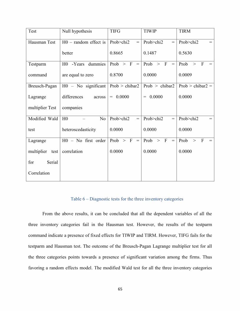
65

Test Null hypothesis TIFG TIWIP TIRM

Hausman Test H0 – random effect is

better

Prob>chi2 =

0.8665

Prob>chi2 =

0.1487

Prob>chi2 =

0.5630

Testparm

command

H0 -Years dummies

are equal to zero

Prob > F =

0.8700

Prob > F =

0.0000

Prob > F =

0.0009

Breusch-Pagan

Lagrange

multiplier Test

H0 – No significant

differences across

companies

Prob > chibar2

= 0.0000

Prob > chibar2

= 0.0000

Prob > chibar2 =

0.0000

Modified Wald

test

H0 – No

heteroscedasticity

Prob>chi2 =

0.0000

Prob>chi2 =

0.0000

Prob>chi2 =

0.0000

Lagrange

multiplier test

for Serial

Correlation

H0 – No first order

correlation

Prob > F =

0.0000

Prob > F =

0.0000

Prob > F =

0.0000

Table 6 – Diagnostic tests for the three inventory categories

From the above results, it can be concluded that all the dependent variables of all the

three inventory categories fail in the Hausman test. However, the results of the testparm

command indicate a presence of fixed effects for TIWIP and TIRM. However, TIFG fails for the

testparm and Hausman test. The outcome of the Breusch-Pagan Lagrange multiplier test for all

the three categories points towards a presence of significant variation among the firms. Thus

favoring a random effects model. The modified Wald test for all the three inventory categories

66

confirms the presence of heteroscedasticity. Finally, the Lagrange multiplier test confirms a lack

of serial correlation for raw materials, finished goods and work-in-progress inventories.

The Hausman test rejects fixed effect models but the testparm command suggests fixed

effect for most of the dependent variables. The Breusch-Pagan Lagrange multiplier also test

supports random effect for all the dependent variables. The selection of models could be a tricky

question and a very subjective issue as per Chen et al. (2005). Therefore, it was preferred to run

regressions for all the models and compare their results for net inventory and the other three

inventory categories.

The results of all the four models for TI, TIFG, TIRM and TIWIP are presented in

the next section. A point to be noted here is that by default, STATA ignores the missing values

and computes the regression tests from the available observations.10

10 http://www.ats.ucla.edu/stat/stata/modules/missing.html

67

5 Results

5.1 Results for net inventory

Table 7 provides the results for the tests run for inventory turnover (TI) of net inventory

for all the four models. The Global F-test of all the four models is less than 0.00001. Hence, all

the models are statistically significant. The R-squared for the fixed effect and least square

dummy models is 0.7649. Hence, these models explain about 76.5% of the variability in the

response variable due to the explanatory variables. The multi-level models, like the mixed effect

model and the random effect model have a hierarchical grouping of the entities which results in

the residuals at each hierarchical level to have a different variance (Gelman el al., 2006). This

implies that each hierarchical level having its own R-squared (Gelman el al., 2006). Hence, the

R-squared for multi-level models is generally not used for evaluating these models (Nakagawa et

al., 2013). Chen et al. (2005) employed fixed effect, mixed effect and random effect models for

their data analysis and do not mention or utilize the R-squared value in case of the mixed effect

and random effect models. Hence, following Chen et al. (2005) in the current study as well, the

R-squared value is utilized for fixed effect model and least square dummy model only.

68

(TI) Inventory turnover – Net inventory

Terms Fixed Effect Random Effect LSDM Mixed effect

Global F – test 0.0000 0.0000 0.0000 0.0000

R-squared 0.7649 0.7649

Year 0.0042787 **

(0.003)

.0037091 **

(0.009)

0.0042787 **

(0.003)

0.0037707 **

(0.008)

GrossMargin -0.0150924 **

(0.000)

-.0149517 **

(0.000)

-0.0150924 **

(0.000)

-0.014966 **

(0.000)

Trevenue

(Firm size)

0.000000003

(0.184)

0.000000004 *

(0.069)

0.000000003

(0.184)

0.000000004 *

(0.076)

CaIn

(Capital

intensity)

-0.0963592

(0.162)

0.0854591

(0.190)

-0.0963592

(0.162)

0.0652729

(0.322)

SGs

(Sales Growth)

0.0687902 **

(0.000)

0.068422 **

(0.000)

0.0687902 **

(0.000)

0.0684661**

(0.000)

**Significant at 5%; *Significant at 10%

Table 7 – Results for net inventory turnover

From Table 7, it is clear that the variables Year, GrossMargin and SG are statistically

significant for all the models. The variable Trevenue is statistically significant for the random

effect and mixed effect models. The coefficient of the variable Year is significant at 5% for all

the four models. The correlation between Year and inventory turnover (TI) for net inventory is

positive and significant. This proves the first part of the Hypothesis 1. Based on the fixed effect

and least square dummy model, it can be said that for every increase of one year in the variable

69

Year, the value of Inventory turnover increases by 0.43%. The mixed effect model states that for

every unit increase in Year, the value of TI increases by 0.38%. Finally, as per the results of the

random effect model, it can be said that the average effect of Year on TI is about 0.37% increase

when Year changes across the companies.

The variable GrossMargin is also significant at 5% for all the models. GrossMargin is

negatively correlated with inventory turnover in all the models. This supports Hypothesis 2 of

the study. Based on the results of the fixed effect model and least square dummy model, it can be

said that for every unit increase in gross margin, the TI decreases by 1.5%. The mixed effect

model indicates that for a unit increase in gross margin, the corresponding decline in IT is 1.4%.

Finally, the results of the random effect model indicate that the average effect of gross margin on

TI is about 1.4% decrease when the gross margin changes across the companies and time.

The variable SG (sales growth) is also statistically significant at 5% for all the models.

SG is positively correlated with inventory turnover in all the models. This supports Hypothesis 5

of the study. All the four models point towards an increase of about 7% in the value of TI for

every unit increase in SG. The variable Trevenue is significant at 10% for random effect and

mixed effect models only. Trevenue is positively correlated with TI supporting Hypothesis 4 of

the current study. However, the impact of Trevenue though positive is negligible on TI. Both,

random effect and mixed effect models suggest that every unit increase in Trevenue leads to an

increase of less than 0.0001% in the value of TI. The coefficients of capital intensity (CaIn) is

not statistically significant in any of the models. Therefore, nothing can be said about the

correlation between TI and CaIn.

70

5.2 Results for Inventory categories

The tests were run for all the three types of inventory categories with statistically

significant results only for work-in-progress inventory. None of the four models were significant

for finished goods and raw materials inventory. Hence, no conclusion can be drawn about the

correlation of their respective inventory turnovers and Year. The results for the time trend of the

work-in-progress inventory is provided in Table 8.

Work in progress – Inventory turnover (TIWIP)

Terms Fixed Effect Random

Effect

LSDM Mixed effect

Global F – test 0.0000 0.0000 0.0000 0.0000

R-squared 0.7023 0.7023

Year 0.0332327 **

(0.000)

0.0324303 **

(0.000)

0.0332327 **

(0.000)

.0324012 **

(0.000)

**Significant at 5%

Table 8 – Results for work-in-progress inventory

Here, all the models are globally significant as indicated by their respective Global F-test

value. The inventory turnover (TIWIP) for work-in-progress inventory is positively correlated

with time proving the second part of Hypothesis 1. The fixed effect model and least square

dummy model explain about 70.23% of the variability in TIWIP due to Year. This is comparable

to the R-squared of the fixed effects and least square dummy models for the net inventory. As

71

per the results of these models for TIWIP, an increase of one year in Year leads to an increase of

3.3% in the value of TIWIP. The mixed effect model suggests an increase of about 3.2% in

TIWIP for every unit increase in Year. The random effect model also points towards an average

impact of Year on TIWIP to be about an increase of 3.2% when Year changes across the

companies.

5.3 Discussion

Based on the above results, it can be concluded that the inventory turnover for net

inventory and work-in-progress inventory has been increasing with time across companies. Since

inventory is inversely proportional to the inventory turnover, the results indicate that the relative

inventory levels for the net inventory and work-in-progress inventory of the Canadian companies

measured in terms of inventory turnover, have been declining over the period from 1987 to 2016.

This answers the main question of this thesis – what was happening to the inventory trends

among the Canadian firms?

This is in line with the findings of Rajagopalan et al. (2001), Boute et al. (2003),

Obermaier (2012), Shan et al. (2013) and Vergin (1998) who all point towards a decline in the

inventory levels for the firms in the countries of their respective study. Table 9 presents a

comparison of the results of some of the published studies with their R-squared and inventory

trends.

72

Paper Study Period R squared Number of firms Time trend -

inventory

Gaur et al. (2005) 1987 – 2000 62.8% - 66.7% 311 Increase

Chen et al. (2005) 1981 – 2000 80% – 86% 7433 Decline

Shan et al. (2013) 2002 – 2009 42.9% – 76.7% 1286 Decline

Johnston (2014) 1982 – 2012 20.14% - 33.89% 126 No long-term

trend

Dehning et al.

(2007)

1994 – 2000 13.5 – 17.3% 123 Decline

Huson and Nanda

(1995)

1980 – 1990 18.44% 55 Decline

Obermaier (2012) 1971 – 2005 67.46% Sector level data Decline

Vs

Current study 1987 – 2016 76.49% 420 Decline

Table 9 – Comparison with previous studies

From the above Table 9, it can be deduced that the R-squared of the current study is equal

or greater than the R-squared of most of the published articles mentioned in the table. Only Chen

et al. (2005) have an R-squared slightly greater than the current study. This shows that the

results of the current study explain a good amount of the variation in the inventories comparable

to most of the other studies. Also, Chen et al. (2005), Obermaier (2012), Shan et al. (2003),

Huson and Nanda (1995) and Dehning et al. (2007) all point towards a decline in total net

inventory as measured by inventory turnover or inventory days or inventory to sales ratios,

73

which is in sync with the results found in the current analysis. Only Gaur et al. (2005) and

Johnston (2014) indicate a deterioration or no trend in inventory levels.

On comparing the total number of firms considered in the studies mentioned in Table 9,

only Chen et al. (2005) and Shan et al. (2003) have a higher number of firms compared to the

current study. One reason is that Chen et al. (2005) and Shan et al. (2003) studied the firms in the

U.S. and China, which are comparatively bigger economies than Canada. In addition to this,

initially in the current study there were 2,523 publicly listed Canadian firms. But only 420 firms

were found to have the required information about net inventory necessary for performing the

time series analysis. Most of the Canadian firms did not report the total net inventory in their

respectively balance sheet and income statement. Even with these limitations, the current study

still has more firms than more than half of the papers investigated in the literature review section.

Hence, based on a good R-squared value of about 76.49% and with 420 firms from across 10

sectors it could be stated that the study is a good representation of the Canadian firms and the

results are significant. This gives a good idea about their inventory trend.

Moving further, in terms of inventory categories, the results point towards a decline in the

work-in-progress inventory for the Canadian companies. No statistically significant results could

be obtained for the raw materials and finished goods inventory of the Canadian firms.

Rajagopalan et al. (2001), Boute et al. (2003), Fullerton et al. (2001) and Chen et al. (2005)

found a decline in work-in-progress and raw materials inventory and no trend in finished goods

inventory. Obermaier (2012) and Cheng et al. (2012) point towards a decline in raw materials

and finished goods inventory. Obermaier (2012) finds an increase in work in progress inventory

whereas Cheng et al. (2012) finds no trend at all for the same.

74

Apart from time trends for the inventory, the current study also finds a negative

correlation between gross margin and inventory turnover (TI) of the net inventory. This supports

that managers do have a trade-off to make between gross margin and inventory turns. A higher

gross margin of the products is associated with lower inventory turns compared to the products

with a lower gross margin (Gaur et al., 2005). This is in line with the results of Gaur et al.

(2005), Shan et al. (2003), Johnston (2014) and Kolias et al. (2011). All of them confirm a

negative correlation between the inventory turnover and the gross margin of a product.

Further, the results of the current analysis of this thesis point towards a negative

correlation between sales growth and relative inventory levels measured in terms of inventory

turnover. Shan et al. (2003) and Rumyantsev et al. (2007) also confirm a negative correlation

between inventory and sales growth. The results of the current study also support a positive

correlation between firm size and inventory turnover. This indicates that with an increase in size

of firms, the inventory levels decline. Larger size of the firms helps in lowering the inventory

through economies of scale. Johnston (2014), Shan et al. (2003) and Rumyantsev et al. (2007)

also find a positive correlation between TI and firm size. However, the impact of the firm size,

though significant, causes a negligible difference in the value of TI for the Canadian firms.

Finally, capital intensity shows a negative correlation with TI in the fixed effect and least square

dummy models, but a positive correlation in the random effect and mixed effect models.

However, since the correlation is not statistically significant in any of the models, nothing can be

confirmed about its correlation with TI. Gaur et al. (2005), Kolias et al. (2011) and Shan et al.

(2003) find a positive correlation between capital intensity and TI, whereas Johnston (2014)

finds a negative correlation between them. Thus, overall the current study finds a confirmation

for Hypotheses 1 2 4 and 5 but no confirmation for the Hypothesis 3.

75

5.4 Sector-level analysis

In this sub-section, a brief discussion on the sector-level analysis for the selected

Canadian firms is provided. The 420 firms selected for the current study belong to the ten sectors

as mentioned in Section 4.1.1. Of these ten sectors, only the manufacturing and mining sectors

have a sufficient number of firms to perform an individual sector level regression. Other sectors

have too few firms, so it would not be feasible to perform panel data analysis for them

separately. Hence, it was decided to assemble the firms of these 10 sectors into three groups.

Using the three-sector theory by Fisher, all the ten sectors can be differentiated into primary,

secondary and tertiary sectors (Schettkat et al., 2003). Companies in the primary sector are

related to the extraction of raw materials which includes agriculture and mining sectors. The

secondary sector includes manufacturing. The companies in the tertiary sector are those related

to services. This group includes retail, warehousing, wholesale, utilities, health care, construction

and food and accommodation sectors. Among them, only the manufacturing and mining sectors

had a sufficient number of firms to allow an individual analysis. Hence, these two sectors were

put in two separate individual groups. The retail, warehousing, wholesale and utilities sectors are

more similar in characteristics compared to the rest. As a result, these four sectors are put

together. The construction sector somewhat closely relates to mining compared to the other

sectors. Consequently, the construction sector is grouped together with the mining sector. The

first group contains only the firms of the manufacturing sector. The second group consists of

companies belonging to the mining and construction sectors. The third group consisted of the

firms from the retail, wholesale, utilities, transportation and warehousing sectors put together.

Three sectors (agriculture and forestry; food and accommodation services; health care

and social assistance) were excluded from the sector level analysis as these sectors had fewer

76

than 10 firms in each of them. Due to such a low number of companies in each of these sectors, it

was not feasible to run regression tests on them individually or in a group put together. Also, it

was not possible to put them in any of the above three groups as the characteristics of these

sectors are considerably different from the latter. The sectoral mix of the groups with the total

number of the firms in each of them is given in Table 10.

Group Number Sectors Total firms

Group 1 Manufacturing 196

Group 2 Mining, Quarrying, Oil and

Gas Extraction;

Construction

115

Group 3 Retail Trade; Transportation

and Warehousing; Utilities;

Wholesale

93

Table 10 – Groups for sector level analysis

The graphical representation of average net inventory against time for the three groups

and the whole dataset together is given in the Table 18 in the Appendix. One limitation of these

graphs is that the earlier years have more missing values compared to the latter. This may impact

the average net inventory values, in-turn impacting the graphical presentation of the inventory

trends in the respective graphical charts. The regression results for the manufacturing sector are

77

provided in the Table 11. The results of the manufacturing sector are similar to the results of the

tests performed for all the sectors together in a single model in the previous sub-section.

Manufacturing sector – inventory turnover (TI)


Global F – test 0.0000 0.0000 0.0000 0.0000

R-squared 0.7522 0.7522

Year 0.0123691 **

(0.000)

0.0119299 **

(0.000)

0.0123691 **

(0.000)

0.0119526 **

(0.000)

GrossMargin -0.009824**

(0.000)

-0.0099926 **

(0.000)

-0.009824 **

(0.000)

-0.0099837 **

(0.000)

Trevenue

(Firm size)

-0.000000003

(0.320)

-0.000000002

(0.589)

-0.000000003

(0.320)

-0.000000002

(0.572)

CaIn

(Capital

intensity)

-.0133046

(0.870)

0.0651182

(0.409)

-.0133046

(0.870)

0 .0611246

(0.438)

SG

(Sales Growth)

0.1816715 **

(0.000)

0.1845235 **

(0.000)

0.1816715 **

(0.000)

0.1843763 **

(0.000)

**Significant at 5%

Table 11 – Results for the manufacturing sector

The results of the Global F-tests indicate that all the four models are significant. The

fixed effect model and the least square dummy models explain about 75.22% of the variability in

inventory turnover due to the explanatory variables. Here, Year has a positive correlation with

78

the inventory turnover, which is significant at 5% for all the models. This supports the first

hypothesis for the public manufacturing companies in Canada. All the four models indicate that

an increase of one year in the Year variable leads to an increase of 1.2% in the value of inventory

turnover for manufacturing firms in Canada. This is a bigger increase compared to the increase

for the complete sample. The GrossMargin is negatively correlated to the inventory turnover and

its coefficient is significant at 5% for all the models. This supports the second hypothesis in case

of the manufacturing firms. As per the results of the fixed effect model and the least square

dummy model, every unit increase in gross margin leads to a decrease of 0.9% in the value of

inventory turnover. The mixed effect and random effect models indicate that the inventory

turnover declines by 1% with a unit increase in gross margin. Further, sales growth (SG) is

positively correlated with inventory turnover in all the models. The fixed effect and least square

dummy models point towards an increase of 19% in the value of TI for a unit increase in SG.

The random effect and mixed effect models indicate about 20% increase in the value of TI with

every unit increase in SG. The results for the correlation between firm size and capital intensity

with inventory turnover is not statistically significant in any of the four models. Thus, overall the

results support the Hypotheses 1 2 and 5 in case of the manufacturing companies.

Table 12 provides the results of the panel data regression for the second group of firms

belonging to the mining and construction sectors.

79

Mining and Construction sectors (Group 2) – inventory turnover (TI)


Global F – test 0.0000 0.0000 0.0000 0.0000

R-squared 0.7644 0.7644

Year 0.0041168

(0.301)

0.0027587

(0.481)

0.0041168

(0.301)

0.0028249

(0.469)


(0.000)

-0.0155032 **

(0.000)

-0.0151329**

(0.000)

-0.0154844 **

(0.000)

Trevenue

(Firm size)

-0.000000002

(0.795)

0.000000005

(0.994)

-0.000000002

(0.795)

-0.000000004

(0.995)

CaIn

(Capital

intensity)

-0.4575172 **

(0.010)

-0.3998421 **

(0.019)

-0.4575172 **

(0.010)

-0.4025894 **

(0.018)

SG

(Sales Growth)

0.0561453 **

(0.000)

0.0551928 **

(0.000)

0.0561453 **

(0.000)

0.0552406 **

(0.000)

**Significant at 5%

Table 12 – Results for mining and construction sectors

The results of the time series regression for Group 2 set of firms belonging to the mining

and construction sectors, show that all the four models are statistically significant. The

coefficients of the variables GrossMargin, sales growth (SG) and capital intensity (CaIn) are

significant. All the models indicate that a unit increase in gross margin would result in 1.5%

decrease in TI. Similarly, the results of the four models show an increase of about 5.7% in TI

80

with a unit increase in SG. For capital intensity, all the models point towards a negative

correlation between TI and CaIn. This is the opposite of the Hypothesis 3, thus disproving it for

the mining and construction sectors. We do not have a clear explanation for this. One possible

reason could be that investments in more warehouses lead to a decentralization of the stock

which requires a higher level of safety stocks. The fixed effect and least square dummy models

point towards a decrease of about 58% in TI for every unit increase in CaIn. Similarly, mixed

effect and random effect models point towards a decline of 49% in the value of TI. The

coefficients of Year and Trevenue are not significant for this group. Overall, the results of Group

2 support Hypotheses 2 and 5, reject Hypothesis 3, while no conclusion can be drawn for

Hypotheses 1 and 4.

Table 13 provides the results for the Group 3 firms belonging to retail, wholesale, utilities

and warehousing and transportation sectors.

81

Retail, Wholesale, Warehousing and Utilities (Group 3) – inventory turnover (TI)


Global F – test 0.0000 0.0000 0.0000 0.0000

R-squared 0.7807 0.7807

Year -0.0048112 *

(0.056)

-0.0050919 **

(0.042)

-0.0048112 *

(0.056)

-0.0050473 **

(0.042)


(0.000)

-0.0221317 **

(0.000)

-0.0228157**

(0.000)

-0.0223323 **

(0.000)

Trevenue

(Firm size)

0.000000013 **

(0.000)

0.000000013 **

(0.000)

0.000000013 **

(0.000)

0.000000013 **

(0.000)

CaIn

(Capital

intensity)

0.049342

(0.756)

0.5405501**

(0.000)

0.049342

(0.756)

0.3786761 **

(0.011)

SG

(Sales Growth)

0.1106174 **

(0.008)

0.1216847**

(0.004)

0.1106174 **

(0.008)

0.1180169 **

(0.004)

**Significant at 5%; *Significant at 10%

Table 13 – Results for retail, wholesale, utilities and warehousing sectors

For Group 3, all the models are significant globally. The variable Year is significant at a

5% level for the mixed effect and random effect models, and significant at 10% level for the

fixed effect and least square dummy models. The variables GrossMargin, Trevenue and SG are

significant at 5% level for all the models. The variable CaIn is significant only in the mixed

effect and random effect models. Here, Year is negatively correlated with TI disapproving the

Hypothesis 1 for Group 3 firms. The fixed effect and least square dummy models indicate a

82

decrease of about 0.48% in TI for every unit increase in Year. The random effect and mixed

effect models point towards a decrease of about 0.5% in TI for unit increase in Year. This shows

that the relative inventory levels measured in terms of TI have been increasing for the firms

belonging to the sectors in Group 3. This is in contrast with the results for the manufacturing

sector and the main results for all the firms in a single model.

The GrossMargin is negatively correlated with TI supporting the Hypothesis 2. All the

models point towards a decline of about 2.2 to 2.3% in the value of TI for every unit increase in

GrossMargin. The variable Trevenue is positively correlated with TI, supporting the Hypothesis

4 for the Group 3 firms. However, the impact of Trevenue on TI is almost negligible in all the

four models. SG is positively correlated with TI for Group 3 firms in all the models supporting

the Hypothesis 5. The results of the four models indicate an increase of about 11.6 to 12.9% in

TI for every unit increase in SG.

Finally, capital intensity (CaIn) is positively correlated to TI in the random effect and

mixed effect models supporting Hypothesis 3 of the current study. The coefficients of CaIn in the

fixed effect and least square dummy models is not statistically significant. The random effect

models states that the average increase in TI is about 71% for every unit increase in CaIn. The

mixed effect model points towards an increase of 46% in TI for a unit increase in CaIn. Overall,

the results for the Group 3 consisting of firms from retail, wholesale, warehousing and utilities

sectors support the Hypotheses 2 3 4 and 5 and disapprove Hypothesis 1.

Comparing the results of all the three groups, it can be said that the relative inventories of

manufacturing sector firms have been declining, whereas the relative inventories of the firms in

retail, wholesale, utilities and warehousing have been increasing over the current study period.

83

No conclusion could be drawn for the mining sector firms. Thus, manufacturing firms support

Hypothesis 1, while Group 3 firms disapprove it. All the three groups agree on a negative

correlation between gross margin and TI supporting Hypothesis 2. Similarly, all the three groups

concur on a positive correlation between SG and TI, supporting Hypothesis 5.

Group 3 firms support the Hypothesis 4, stating a positive correlation between the firm

size and TI. This is also in line with the main results of section 4.1. Finally, for capital intensity

group 2 firms show a negative correlation with TI, rejecting Hypothesis 3; whereas firms in

group 3 indicate a positive correlation between CaIn and TI, supporting Hypothesis 3. The

manufacturing firms in Group 1 show no significant results for the firm size and capital intensity.

The above results show that the relative inventories, measured in terms of the inventory

turnover, have been showing a declining trend for the firms in the Canadian manufacturing

sector. This is in consonance with the findings of Rajagopalan et al. (2001), Chen et al. (2005),

Obermaier (2012), Robb et al. (2012), Boute et al. (2003), Shah et al. (2007), Huson and Nanda

(1995) and Mishra et al. (2013). All these authors confirm a decline in the relative inventory

levels for the manufacturing sectors or manufacturing firms in their respective studies. In

contrast to the above, the firms belonging to retail and wholesale sectors in Group 3 point

towards an increasing trend in their relative inventory levels measured in terms of inventory

turnover. Chen et al. (2007) and Irvine (2003) point towards an improvement in the relative

inventory levels for the wholesale sector whereas Shah et al. (2007) indicates a deterioration of

the same. Irvine (2003) and Boute et al. (2003) point towards a decline in the relative inventory

levels for the retail sector, but Shah et al. (2007), Gaur et al. (2005), Johnston (2014), Kolias et

al. (2011) conclude a deterioration or no trend in the relative inventory levels for the retail sector.

84

6 Conclusion

This thesis primarily investigated the time trends for the relative inventory levels in terms

of inventory turnover of the net inventory and the three inventory categories, namely raw

material, work-in-progress and finished goods inventory, for 420 publicly listed Canadian firms

for the period from 1987 to 2016. Additionally, correlations of the gross margin, capital

intensity, sales growth and firm size with net inventory were also analyzed. Based on the

reported results, it can be concluded that the relative inventory levels of the publicly listed

Canadian firms have been declining from 1987 to 2016. The decline has been found for net

inventory as well as for work-in-progress inventory. The results help to clarify the question of

what happened to inventory trends in the case of Canadian firms. There was a lack of

investigation of Canadian firms in particular; in almost all of the academic studies concerning the

inventory trends. Performing a time series analysis, the current study indicates a declining trend

for Canadian firms. Apart from inventory trends, a significant positive correlation is found

between the inventory and the gross margin of the products. Also, the correlation between the

firm size and sales growth with inventory is found to be negative. However, no statistically

significant results are found for capital intensity.

Additionally, at the sector level analysis, the results confirm a decline in the inventory

trends for Canadian firms belonging to the manufacturing sector, but an increase in the inventory

levels for Canadian firms belonging to retail, wholesale, warehousing and utilities sectors. No

significant result is found for the inventory levels of the firms belonging to mining and

construction sectors. The results of all the sectors confirm a positive correlation between the

gross margin and the inventory and a negative correlation between sales growth and the

85

inventory. Only firms from the retail, wholesale, warehousing and utilities sectors show a

negative correlation between the firm size and the inventory. For capital intensity, the mining

and construction sectors show a positive correlation, whereas retail, wholesale, warehousing and

utilities sectors show a negative correlation with the inventory.

The biggest limitation of this study is the limited amount of data. A large number of the

Canadian firms did not provide inventory data in their respective balance sheets and income

statements. Out of the total 2,523 Canadian firms from ten industries, only 420 firms had

declared enough inventory to allow panel data analysis. Another 300 firms did have inventory

data but had too many missing values for many of the years of the studied period (1987–2016).

Despite this limitation, the current study provides statistically significant results answering the

research question. Another limitation was that the majority of the Canadian firms in our sample

either belonged to manufacturing or mining sectors. Thus, this could result in bias as a larger

share of manufacturing and mining industries could impact the outcome of the firms in other

industries. Moreover, due to the smaller number of firms in sectors other than manufacturing and

mining, it was not feasible to conduct an individual sector level analysis. In addition to the

above, it could be interesting if the data about inventory for Canadian firms could be obtained for

the period prior to 1987. Lastly, the current research could be further improved by performing

firm level analysis by introducing dummy variables for representing the sectors in the current

model.

This study provides a base for further analysis of inventory trends for Canadian

companies. A time series analysis can be performed along similar lines to the current study on a

dataset containing more Canadian firms obtained from another data source other than the Osiris

database and having much more complete information. It would be interesting to compare both

86

the results. Another approach could be to perform an aggregate sector level analysis instead of

firm level for the Canadian economy to understand inventory trends. Future researchers could

also correlate the inventory performance with the financial performance of Canadian firms. In

addition to that, researchers could try to analyze the impact of various factors like supplier co-

ordination, information technology, globalization etc., on inventory trends not taken into

consideration in the current study due to a lack of information. Lastly, it could be interesting to

find more firms with required data in the sectors other than the manufacturing sector and analyze

their inventory behavior and compare them. This investigation could further be extended to the

sub-sector level within a sector provided adequate data is available for such an analysis.

87

Bibliography

Books:

Shingo, S., & Dillon, A. P. (1989). "The Principles of the Toyota Production System" in A study

of the Toyota production system: From an Industrial Engineering Viewpoint. CRC Press, p.67-

95

Thompson, James D. "Rationality in Organizations" in Organizations in action, McGraw Hill,

1997, p. 14-24

Waller, M. A., & Esper, T. L. (2014). The Definitive Guide to Inventory Management: Principles

and Strategies for the Efficient Flow of Inventory Across the Supply Chain. Pearson Education,

p. 1-27

Published Articles:

Alejo, J., Galvao, A., Montes-Rojas, G., & Sosa Escudero, W. (2015). Tests for normality in

linear panel data models. Documentos de Trabajo del CEDLAS.

http://sedici.unlp.edu.ar/handle/10915/51201

Amihud, Y., & Medenelson, H. (1989). Inventory behaviour and market power: an empirical

investigation. International Journal of Industrial Organization, 7(2), 269-280.

Benoit, K. (2011). Linear regression models with logarithmic transformations. London School of

Economics, London, 1-8. http://www.kenbenoit.net/courses/ME104/logmodels2.pdf

Blazenko, G. W., & Vandezande, K. (2003). Corporate holding of finished goods inventories.

88

Journal of Economics and Business, 55(3), 255–266.

Boute, R., Lambrecht, M., & Lambrechts, O. (2003). Did inventories decrease in the Belgian

manufacturing sector between 1979 and 2000? DTEW Research Report 0352, 1–15.

Cannon, A. R. (2008). Inventory improvement and financial performance. International Journal

of Production Economics, 115(2), 581–593.

Chen, H., Frank, M. Z., & Wu, O. Q. (2005). What Actually Happened to the Inventories of

American Companies Between 1981 and 2000? Management Science, 51(7), 1015–1031.

Chen, H., Frank, M. Z., & Wu, O. Q. (2007). U.S. Retail and Wholesale Inventory Performance

from 1981 to 2004. Manufacturing & Service Operations Management, 9(4), 430–456.

Cheng, L. C. V., Cantor, D. E., Dresner, M., & Grimm, C. M. (2012). The impact of contract

manufacturing on inventory performance: An examination of U.S. manufacturing industries.

Decision Sciences, 43(5), 889–928.

de Leeuw, S., Holweg, M., & Williams, G. (2011). The impact of decentralised control on

firm‐level inventory: evidence from the automotive industry. International Journal of

Physical Distribution & Logistics Management, 41(5), 435–456.

Dehning, B., Richardson, V. J., & Zmud, R. W. (2007). The financial performance effects of IT-

based supply chain management systems in manufacturing firms. Journal of Operations

Management, 25(4), 806–824.

Demeter, K. (2003). Manufacturing Strategy and competitiveness. International Journal of

Production Economics, 81-82, 205–213.

89

Demeter, K., & Matyusz, Z. (2011). The impact of lean practices on inventory turnover.

International Journal of Production Economics, 133(1), 154–163.

Fullerton, R. R., Fullerton, R. R., Mcwatters, C. S., & Mcwatters, C. S. (2001). The production

performance benefits from JIT implementation. Journal of Operations Management, 19,

81–96.

Gaur, V., Fisher, M. L., & Raman, A. (2005). An Econometric Analysis of Inventory Turnover

Performance in Retail Services. Management Science, 51(2), 181–194.

Gelman, A., & Pardoe, I. (2006). Bayesian Measures of Explained Variance and Pooling in

Multilevel (Hierarchical) Models. Technometrics, 48(2), 241–251.

Han, C., Dresner, M., & Windle, R. J. (2008). Impact of global sourcing and exports on US

manufacturing inventories. International Journal of Physical Distribution and Logistics

Management, 38(6), 475–494.

Huson, M., & Nanda, D. (1995). The impact of just-in-time manufacturing on firm performance

in the US. Journal of Operations Management, 12(3–4), 297–310.

Irvine, F. O. (2003). Long term trends in US inventory to sales ratios. International Journal of

Production Economics, 81–82, 27–39.

Irvine, F. O. (2005). Trend breaks in US inventory to sales ratios. International Journal of

Production Economics, 93, 13–23.

Jain, N., Girotra, K., & Netessine, S. (2014). Managing global sourcing: Inventory performance.

Management Science, 60(5), 1202–1222.

90

Johnston, A. (2014). Trends in retail inventory performance: 1982 – 2012. Operations

Management Research, 7(3–4), 86–98.

Kolias, G. D., Dimelis, S. P., & Filios, V. P. (2011). An empirical analysis of inventory turnover

behaviour in Greek retail sector: 2000-2005. International Journal of Production

Economics, 133(1), 143–153.

Kros, J. F., Falasca, M., & Nadler, S. S. (2006). Impact of just-in-time inventory systems on

OEM suppliers. Industrial Management & Data Systems, 106(2), 224–241.

Lieberman, M. B., & Demeester, L. (1999). Inventory Reduction and Productivity Growth:

Linkages in the Japanese Automotive Industry. Management Science, 45(4), 466–485.

Lieberman, M. B., Helper, S., & Demeester, L. (1999). The empirical determinants of inventory

levels in high-volume manufacturing. Production and Operations Management, 8, 44–55.

Mishra, S., Modi, S. B., & Animesh, A. (2013). The relationship between information

technology capability, inventory efficiency, and shareholder wealth: A firm-level empirical

analysis. Journal of Operations Management, 31(6), 298–312.

Montes-Rojas, G., & Sosa-Escudero, W. (2011). Robust tests for heteroskedasticity in the one-

way error components model. Journal of Econometrics, 160(2), 300-310.

Nakagawa, S., & Schielzeth, H. (2013). A general and simple method for obtaining R2 from

generalized linear mixed‐effects models. Methods in Ecology and Evolution, 4(2), 133-142.

Obermaier, R. (2012). German inventory to sales ratios 1971-2005 - An empirical analysis of

business practice. International Journal of Production Economics, 135(2), 964–976.

91

Torres-Reyna, O. (2007). Panel data analysis fixed and random effects using Stata (v. 4.2). Data

& Statistical Services, Princeton University.

https://www.princeton.edu/~otorres/Panel101.pdf

Rajagopalan, S., & Malhotra, A. (2001). Have U . S . Manufacturing Inventories Really

Decreased? An Empirical Study. Manufacturing & Service Operations Management, 3(1),

14–24.

Robb, D. J., Liu, F., Lai, R., & Ren, Z. J. (2012). Inventory in mainland China: Historical,

industry, and geographic perspectives. International Journal of Production Economics,

135(1), 440–450.

Rumyantsev, S., & Netessine, S. (2007). What Can Be Learned from Classical Inventory

Models? A Cross-Industry Exploratory Investigation. Manufacturing & Service Operations

Management, 9(4), 409–429.

Schettkat, R., & Yocarini, L. (2003). The shift to services: a review of the literature. Retrived

from http://ftp.iza.org/dp964.pdf

Shah, R., & Shin, H. (2007). Relationships among information technology, inventory, and

profitability: An investigation of level invariance using sector level data. Journal of

Operations Management, 25(4), 768–784.

Shan, J., & Zhu, K. (2013). Inventory management in China: An empirical study. Production

and Operations Management, 22(2), 302–313.

StataCorp. (2013). Stata Multilevel mixed-effects reference manual.

Swamidass, P. M. (2007). The effect of TPS on US manufacturing during 1981 – 1998 :

92

inventory increased or decreased as a function of plant performance. International Journal

of Production Research, 45(16), 3763–3778.

Vergin, R. (1998). An examination of inventory turnover in the Fortune 500 industrial

companies. Production and Inventory Management Journal, 39(1), 51–56.

Williams, R. (2015). Heteroscedasticity. University of Notre Dame, 1–16.

https://www3.nd.edu/~rwilliam/stats2/l25.pdf

Links:

HEC online library – Osiris user guide

https://proxy2.hec.ca:3090/version-2016628/Search.QuickSearch.serv?_CID=1&context=

35TZCN8NR6T9HQ1

http://www.investopedia.com/ask/answers/122214/what-difference-between-revenue-and-

sales.asp

http://dictionary.cambridge.org/dictionary/english/inventory

http://www.referenceforbusiness.com/management/Int-Loc/Inventory-Types.html

http://www.ats.ucla.edu/stat/stata/modules/missing.html

http://www.ats.ucla.edu/stat/stata/webbooks/reg/chapter4/statareg4.htm

http://mining.ca/resources/mining-facts

93

Appendix

Sectors selected for the current study No Sector Sub-sectors 1 Agriculture, Forestry,

Fishing and Hunting

Crop production; Animal production and aquaculture; Forestry and logging; Fishing, hunting and trapping; Support activities for agriculture and forestry.

2 Construction Construction of buildings; Heavy and civil engineering construction; Specialty trade contractors.

3 Manufacturing Food manufacturing; Beverage and tobacco product manufacturing; Textile mills; Textile product mills; Apparel manufacturing; Leather and allied product manufacturing; Wood product manufacturing; Paper manufacturing; Printing and related support services; petroleum and coal products manufacturing; Chemical manufacturing; Plastics and rubber products manufacturing; Nonmetallic mineral product manufacturing; primary metal manufacturing; Fabricated metal product manufacturing; Machinery manufacturing; Computer and electronic product manufacturing; Electrical equipment, appliance and component manufacturing; Transportation equipment manufacturing; Furniture and related product manufacturing; Miscellaneous manufacturing.

4 Mining, Quarrying, Oil and Gas exploration

Oil and gas extraction; Mining (except oil and gas); Support activities for mining.

5 Retail Trade Motor vehicle and parts dealers; Furniture and Home Furnishings Stores; Electronics and Appliance Stores; Building Material and Garden Equipment and Supplies Dealers; Food and Beverage Stores; Health and Personal Care Stores; Gasoline Stations; Clothing and Clothing Accessories Stores; Sporting Goods, Hobby, Musical Instrument, and Book Stores; General Merchandise Stores; Miscellaneous Store Retailers; Nonstore Retailers.

6 Transportation and Warehousing

Air Transportation; Rail Transportation; Water Transportation; Truck Transportation; Transit and Ground Passenger Transportation; Pipeline Transportation; Scenic and Sightseeing Transportation;

94

Support Activities for Transportation; Postal Service; Couriers and Messengers; Warehousing and Storage.

7 Health Care and Social Assistance

Ambulatory Health Care Services; Hospitals; Nursing and Residential Care Facilities; Social Assistance.

8 Accommodation and Food Services

Accommodation; Food Services and Drinking Places.

9 Utilities Utilities.

10 Wholesale Trade Merchant Wholesalers, Durable Goods; Merchant Wholesalers, Nondurable Goods; Wholesale Electronic Markets and Agents and Brokers.

Table 14 – Sectors and sub-sectors included in the current study

95

Sectors excluded from the current study No Sector Sub-sectors 1 Information Publishing Industries (except Internet); Motion Picture

and Sound Recording Industries; Broadcasting (except Internet); Telecommunications; Data Processing, Hosting, and Related Services; Other Information Services.

2 Finance and Insurance Monetary Authorities-Central Bank; Credit Intermediation and Related Activities; Securities, Commodity Contracts, and Other Financial Investments and Related Activities; Insurance Carriers and Related Activities; Funds, Trusts, and Other Financial Vehicles.

3 Real Estate and Rental and Leasing

Real Estate; Rental and Leasing Services; Lessors of Nonfinancial Intangible Assets (except Copyrighted Works).

4 Professional, Scientific, and Technical Services

Professional, Scientific, and Technical Services.

5 Management of Companies and Enterprises

Management of Companies and Enterprises.

6 Administrative and Support and Waste Management and Remediation Services

Administrative and Support Services; Waste Management and Remediation Services.

7 Educational Services

Educational Services.

8 Arts, Entertainment, and Recreation

Performing Arts, Spectator Sports, and Related Industries; Museums, Historical Sites, and Similar Institutions; Amusement, Gambling, and Recreation Industries.

9 Public Administration Executive, Legislative, and Other General Government Support; Justice, Public Order, and Safety Activities; Administration of Human Resource Programs; Administration of Environmental Quality Programs; Administration of Housing Programs, Urban Planning, and Community Development; Administration of Economic Programs; Space Research and Technology; National Security and International Affairs.

Table 15 – Sectors and sub-sectors excluded in the current study

96

No Variables No. Of

observations

Mean Standard

deviation

Skewness Kurtosis

1 Inventory

turnover

6,682 23.78 326.76 38.43 1,681.03

2 Gross Margin 6,872 35.64 22.92 0.28 3.90

3 Trevenue 7,292 1,993,521 5,424,094 4.64 27.51

4 Sales growth

(SG)

6,723 -0.90 4.03 -43.12 2,093.39

5 Capital

intensity (CaIn)

7,422 0.58 0.24 -0.42 2.23

Table 16 – Summary of the variables

97

Variables Unlogged histogram Natural log histogram Trevenue

Gross Margin

Sales growth (SG)

Capital

0

500

1000

1500

2000

2500

0 5 10 15 20

Trevenue

0

100

200

300

400

500

600

0 10 20 30 40

log of Trevenue

0

50

100

150

200

0 50 100 150 200 250

GrossMargin

0

500

1000

1500

2000

0 5 10 15 20

log of GrossMargin

0

1000

2000

3000

4000

5000

0 50 100 150 200 250

Sales Growth

0

200

400

600

800

1000

0 5 10 15 20 25

log of Sales Growth

98

Intensity (CaIn)

Table 17 – Histogram of explanatory variables

0

200

400

600

800

1000

1200

1400

0 5 10 15

Capital Intensity

0

200

400

600

800

0 5 10 15 20

log of Capital Intensity

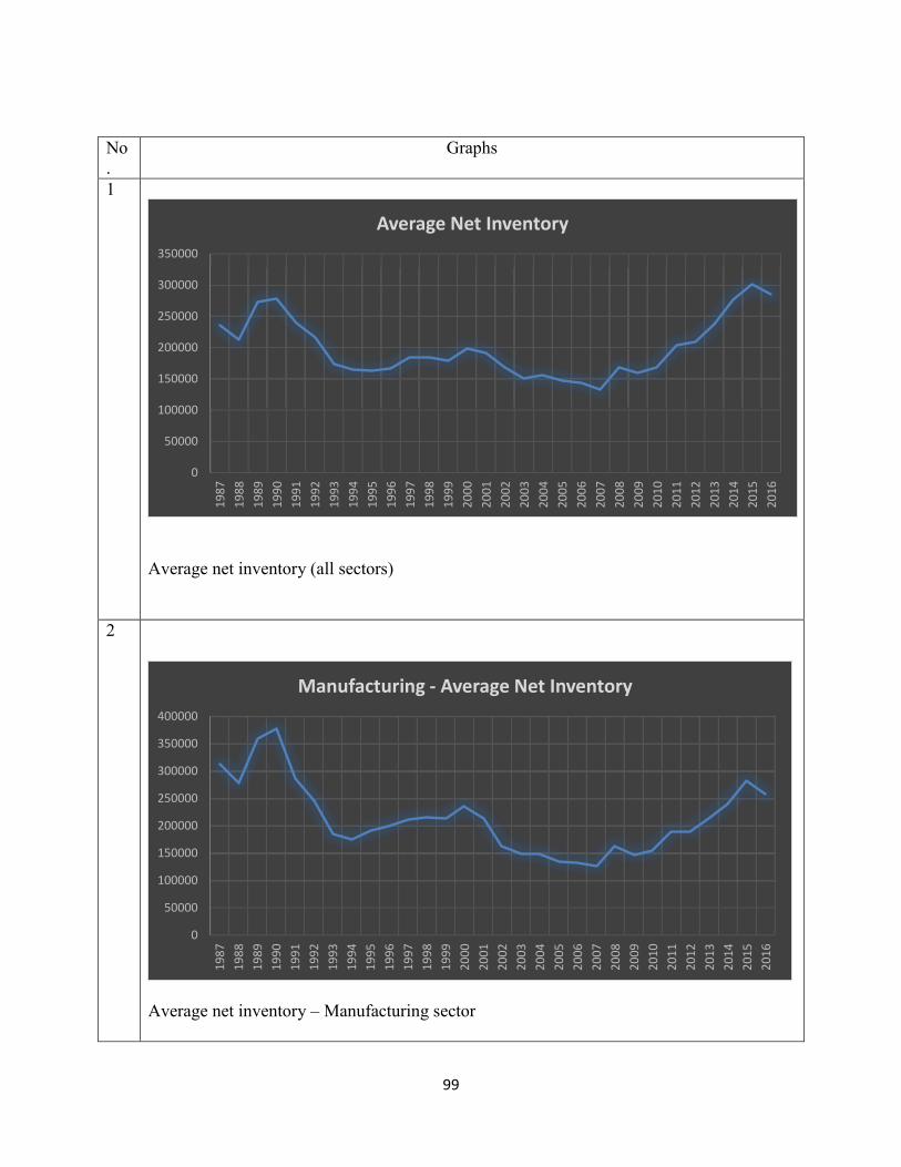
99

0

50000

100000

150000

200000

250000

300000

350000

19

87

19

88

19

89

19

90

19

91

19

92

19

93

19

94

19

95

19

96

19

97

19

98

19

99

20

00

20

01

20

02

20

03

20

04

20

05

20

06

20

07

20

08

20

09

20

10

20

11

20

12

20

13

20

14

20

15

20

16

Average Net Inventory

0

50000

100000

150000

200000

250000

300000

350000

400000

19

87

19

88

19

89

19

90

19

91

19

92

19

93

19

94

19

95

19

96

19

97

19

98

19

99

20

00

20

01

20

02

20

03

20

04

20

05

20

06

20

07

20

08

20

09

20

10

20

11

20

12

20

13

20

14

20

15

20

16

Manufacturing - Average Net Inventory

100

0

50000

100000

150000

200000

250000

19

87

19

88

19

89

19

90

19

91

19

92

19

93

19

94

19

95

19

96

19

97

19

98

19

99

20

00

20

01

20

02

20

03

20

04

20

05

20

06

20

07

20

08

20

09

20

10

20

11

20

12

20

13

20

14

20

15

20

16

Mining & Construction - Average Net Inventory

0

100000

200000

300000

400000

500000

600000

19

87

19

88

19

89

19

90

19

91

19

92

19

93

19

94

19

95

19

96

19

97

19

98

19

99

20

00

20

01

20

02

20

03

20

04

20

05

20

06

20

07

20

08

20

09

20

10

20

11

20

12

20

13

20

14

20

15

20

16

Retail, Wholesale, Wareshousing & Utilities - Average Net Inventory

101

STATA outputs for net inventory

Fixed effect model

Random Effect model

102

Least square dummy model

Mixed effect model

103

STATA outputs for work-in-progress inventory

Fixed effect model

Random Effect model


104

Mixed effect model

Stata outputs for manufacturing sector

Fixed effect model

105

Random effect model


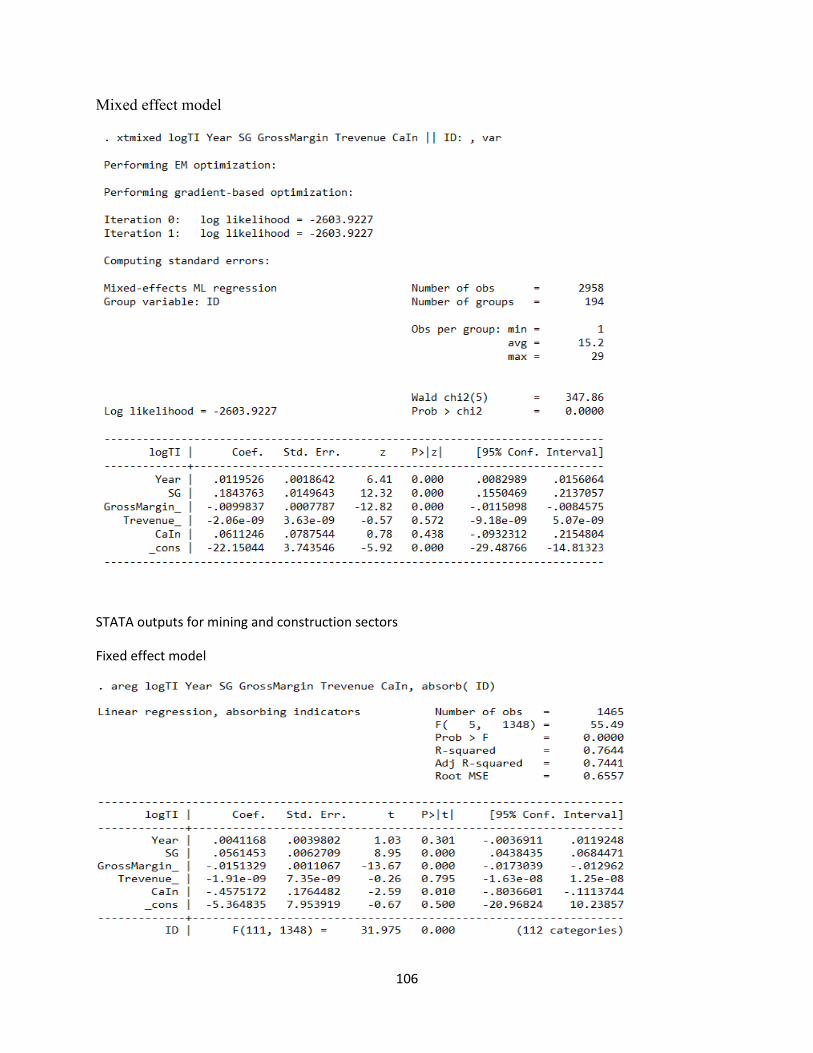
106

Mixed effect model

STATA outputs for mining and construction sectors

Fixed effect model

107

Random effect model


108

Mixed effect model

STATA outputs for retail, wholesale, utilities and warehousing sectors

Fixed effect model

109

Random Effect Model

Least Square Dummy Model

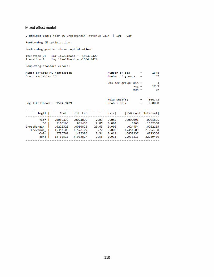
110

Mixed effect model

HEC Montréal Analysis of Inventory Levels of Canadian ...party logistics, information technology,...

Documents

Transcript of HEC Montréal Analysis of Inventory Levels of Canadian ...party logistics, information technology,...