
Heavy Truck Cooper ative Adaptive Cruise Control:...
138
Page 1 of 138 Heavy Truck Cooperative Adaptive Cruise Control: Evaluation, Testing, and Stakeholder Engagement for Near Term Deployment: Phase Two Final Report April 4 th , 2017 Auburn University American Transportation Research Institute Meritor WABCO Peloton Technology Peterbilt Trucks
Transcript of Heavy Truck Cooper ative Adaptive Cruise Control:...

Page 1 of 138
Heavy Truck Cooperative Adaptive Cruise Control: Evaluation, Testing, and Stakeholder Engagement for Near Term Deployment: Phase Two Final Report
April 4th, 2017
Auburn University American Transportation Research Institute Meritor WABCO Peloton Technology Peterbilt Trucks

Page 2 of 138
Technical Report Documentation Page 1. Report No. FHWA-
2. Government Accession No.
3. Recipient’s Catalog No.
4. Title and Subtitle Heavy Truck Cooperative Adaptive Cruise Control: Evaluation, Testing, and Stakeholder Engagement for Near Term Deployment: Phase Two Final Report
5. Report Date April 4th, 2017
6. Performing Organization Code
7. Author(s) Auburn: Dr. David Bevly (GAVLAB), Dr. Chase Murray (ISE-MW), Dr. Alvin Lim (CSSE), Dr. Rod Turochy (ISE), Dr. Richard Sesek (OSE), Scott Smith (GAVLAB), Luke Humphreys (ARG) Grant Apperson (GAVLAB), Jonathan Woodruff (ISE-MW), Song Gao (CSSE), Mikhail Gordon (ISE), Nicholas Smith (OSE), Shraddha Praharaj, Dr. Joshua Batterson (ARG), Richard Bishop (Bishop Consulting) ATRI: Daniel Murray Meritor WABCO: Alan Korn Peloton Technology: Dr. Josh Switkes, Stephen Boyd Peterbilt Trucks: Bill Kahn
8. Performing Organization Report No.
9. Performing Organization Name And Address Auburn University Department of Mechanical Engineering 1418 Wiggins Hall Auburn University, AL 36849-5341
10. Work Unit No. (TRAIS)
11. Contract or Grant No.
12. Sponsoring Agency Name and Address Federal Highway Administration 1200 New Jersey Ave, SE Washington, DC 20590
13. Type of Report and Period Covered Task Report, December 2014 – August 2016 14. Sponsoring Agency Code
15. Supplementary Notes Contracting Officer's Technical Representative: Kevin Dopart
16. Abstract Under the FHWA Exploratory Advanced Research project “Heavy Truck Cooperative Adaptive Cruise Control: Evaluation, Testing, and Stakeholder Engagement for Near Term Deployment” this document provides a summary of Phase Two results for evaluating the commercial feasibility of Driver Assistive Truck Platooning (DATP).
DATP is a form of Cooperative Adaptive Cruise Control for heavy trucks (two-truck platoons). DATP takes advantage of increasing maturity of vehicle-to-vehicle (V2V) communications, plus widespread deployment of DSRC-based V2V connectivity expected over the next decade, to improve freight efficiency, fleet efficiency, safety, and highway mobility, plus reduce emissions. Notably, truck fleets can proceed with implementing DATP regardless of the regulatory timeline for DSRC.
Phase Two consisted of further investigations into topics explored in Phase One. Included in the analysis is a testing program of the DATP prototype (including detailed SAE Type II Fuel Economy testing), wireless communications optimization, traffic modeling to understand the impact on roadways at various levels of market penetration, and analysis of methods to find DATP linking partners, as well as aerodynamic simulations to understand the drag performance evident on the vehicles. In particular, the report includes a detailed analysis of the fuel economy testing data.
17. Key Words
18. Distribution Statement
19. Security Classif. (of this report)
20. Security Classif. (of this page)
21. No. of Pages
22. Price
Form DOT F 1700.7 (8-72) Reproduction of completed page authorized

Page 3 of 138
I.Contents
I. Contents ................................................................................................................................................................................ 3
II. Executive Summary ............................................................................................................................................................. 5
A.ReviewofPhaseOneActivities..................................................................................................................................6B.PhaseTwo:KeyFindings..............................................................................................................................................71. DATPBusinessCaseAnalysis..........................................................................................................................72. DATPInter-vehicleAerodynamicsModeling.............................................................................................73. TestTrackEvaluationofSystemFuelEconomy........................................................................................94. AnalysisofWirelessCommunicationsCharacteristicsWithArticulatedTractor-Trailers....105. DATPPlatoonFormationStrategiesEvaluation....................................................................................116. TrafficFlowandMobilityImpacts..............................................................................................................11
C.ConclusionandRecommendations.......................................................................................................................12III. Introduction ...................................................................................................................................................................... 14
D.Partners............................................................................................................................................................................151. AmericanTransportationResearchInstitute(ATRI)..........................................................................152. PelotonTechnology.........................................................................................................................................153. PeterbiltTrucks................................................................................................................................................154. MeritorWABCO.................................................................................................................................................155. AuburnUniversity............................................................................................................................................16
IV. User and Business Case Evaluation ................................................................................................................................. 17
A.Introduction....................................................................................................................................................................17B.Process..............................................................................................................................................................................17C.Discussion........................................................................................................................................................................18D.SummaryandObservations.....................................................................................................................................23
V. Vehicle Preparations and Systems Testing ........................................................................................................................ 25
A.InstallationofPelotonDATPSystem...................................................................................................................25B.Closed-CourseFuelEconomyTestingofDATPSystem...............................................................................291. LateralOffsetAnalysis....................................................................................................................................312. ControllerDither..............................................................................................................................................323. EngineTemperature........................................................................................................................................344. GeneralResultsandConclusions................................................................................................................35
VI. V2V Wireless Communications ....................................................................................................................................... 36
A.DSRCRadioPerformanceTest................................................................................................................................361. BackgroundonReal-worldDSRCRadios.................................................................................................362. DSRCTestingPlan............................................................................................................................................363. DesignandImplementationoftheTestProgram.................................................................................374. StaticTestingResults......................................................................................................................................395. DynamicTestsfromNCATTrack................................................................................................................46

Page 4 of 138
B.InterframeCompressionTransmissionLayer.................................................................................................531. ProblemAnalysis–AnExtremeCaseStudy.............................................................................................532. DesignoftheAlgorithm..................................................................................................................................543. ImplementationandExperimentalSetup................................................................................................564. FirstGlance.........................................................................................................................................................585. AdaptiveICTL.....................................................................................................................................................586. Conclusion...........................................................................................................................................................62
VII. DATP Inter-Vehicle Aerodynamics Research ................................................................................................................ 63
A.Two–VehicleModeling.............................................................................................................................................63B.MultipleGeometries....................................................................................................................................................65C.Three-VehiclePlatoons..............................................................................................................................................67D.Lateraloffset...................................................................................................................................................................68E.Conclusion........................................................................................................................................................................72
VIII. Finding Linking Partners: Analysis and Methods ......................................................................................................... 73
F.Introduction.....................................................................................................................................................................731. ReviewofPhaseOneFindings......................................................................................................................752. SensitivityAnalysis..........................................................................................................................................78
G.PhaseTwoAnalysisSummaryResults................................................................................................................87IX. Potential Traffic Flow and Mobility Impacts ................................................................................................................... 98
A.Methodology...................................................................................................................................................................98B.Results.............................................................................................................................................................................100
X. Conclusion and Recommendations .................................................................................................................................. 108
XI. Appendix A .................................................................................................................................................................... 110
Figure 93: Average Error of Measured Following Distance v. Following Distance ........................................................... 121Figure 101: Fuel rate for the set of runs v. following distance for the lead truck ................................................................ 124
Figure 118: Dewpoint v. Following Distance ...................................................................................................................... 129
Figure 119: Heat Index v. Following Distance .................................................................................................................... 129Figure 120: Humidity v. Following Distance ...................................................................................................................... 130
XII. References ..................................................................................................................................................................... 138

Page 5 of 138
II. Executive Summary
The FHWA Exploratory Advanced Research project “Heavy Truck Cooperative Adaptive Cruise Control: Evaluation, Testing, and Stakeholder Engagement for Near Term Deployment,” led by Auburn University, is performing research and evaluation to assess the commercial viability of truck platooning in long and regional haul operations. Joining Auburn University on the team are partners Peloton Technology, Peterbilt Trucks, Meritor WABCO, and the American Transportation Research Institute (ATRI) (a research organization within the American Trucking Associations Federation). The lead organization within Auburn is the GPS and Vehicle Dynamics Laboratory (GAVLAB).
For the particular form of Cooperative Adaptive Cruise Control (CACC) addressed here, the term “Driver Assistive Truck Platooning” (DATP) has been developed to support stakeholder engagement with the trucking industry. In DATP, two or more trucks are exchanging data, with one truck leading and the other truck(s) closely following the leader. The technology basis includes radar (for longitudinal sensing), DSRC-based V2V communications (for low latency exchange of vehicle performance parameters between vehicles), satellite positioning (sufficient to discriminate in-lane communications from out-of-lane communications), actuation (for vehicle longitudinal control), and human-machine interfaces (with distinct modes for leading or following). As an SAE Level 1 Automated system, only longitudinal control is automated; the driver remains fully responsible for steering and has the ability to override system brake or throttle commands at any time1.
DATP builds on Adaptive Cruise Control (ACC), which has been available to the trucking industry for several years. Approximately 100,000 ACC-equipped Class 8 trucks are on the road now in the United States. DATP has significant positive fuel savings potential for heavy truck operations beyond what ACC can deliver alone. DATP could also increase safety by extending the functionality of forward collision mitigation systems (CMS), and may provide fleet users with extra incentives for CMS adoption due to prospective safety and fuel savings.
Long haul trucking represents more than 10% of US oil use, with fuel representing 41% of fleet operating expense2,3. Previous testing has shown that due to aerodynamic drafting effects, DATP has the potential to significantly reduce fuel use: on the order of 4% for the lead truck and 10% for the following truck4.
In terms of safety, the radar-based system provides an additional level of situational awareness to the driver whether DATP is activated or not. The most common highway accident for heavy trucks is frontal collisions. A DATP system can actively mitigate these types of accidents without relying on driver reaction time. This provides faster, more reliable, and more accurate reactions to upcoming hazards by the following truck than is available from a driver or current systems.
Notably, truck fleets can proceed with implementing DATP in the near term regardless of the regulatory timeline for DSRC.
This research focuses on investigating business factors of DATP operations and the extent of potential reductions in fuel consumption, as well as safety and other impacts. Our starting hypothesis was that “DATP technology is near market-ready for industrial use and will provide value in specific roadway and operating conditions for heavy truck fleet operations.” Throughout both phases of the project, this research has attempted to address this hypothesis and resolve issues related to near-term deployment.
This document provides a summary of the Phase Two results towards this goal. It attempts to address industry needs for the system, as well as anticipating the needs of other highway travelers in regards to traffic flow and safety. Phase Two built upon Phase One results and consisted of the following elements:
a. Business case investigations: performing interviews with key fleet executives to assess their views of factors critical to commercial feasibility.
b. System testing: equipping the Peterbilt tractors with a Peloton prototype DATP system plus data acquisition equipment, followed by performance testing at the test track in the areas of wireless communications, vehicle control, positioning, and safety.
c. Wireless communications: on-track testing to stress the DSRC system, which was evaluated for packet loss, message delay, channel congestion, and other performance indices. Algorithms and protocols were designed that may improve scalability of DSRC.
d. Aerodynamics modeling: developing models with greater detail to support more in-depth evaluations. This included platoons of more than two vehicles. These models were integrated with vehicle models.

Page 6 of 138
e. Platoon formation: further modeling with regard to assessing platoon formation included extending the analysis of ATRI-provided truck data for additional highway corridors, and incorporating differences in fuel economy benefits depending on platoon position.
f. Traffic impacts evaluation: modeling a 5.3-mile segment of Interstate 85 in Alabama through a small urban area that includes three interchanges during the peak hour of truck traffic (rather than the peak hour of total traffic, which was modeled in Phase One). Also, DATP effects for a freeway section without interchanges, as well as an isolated of a freeway interchange, were investigated.
In summary, the objective of this research was to perform the necessary technical work, evaluation, and industry engagement to identify the key questions that must be answered prior to market introduction of heavy truck DATP, and to begin to answer those questions. Based on fuel economy improvements observed in testing, a strong business case exists for introducing this technology within the trucking industry.
During Phases One and Two, the research team identified these key questions and converted them into a concept of operations and high level system requirements which can serve as a guide to system developers. At a technical level, research results from the items noted above have broadened the body of knowledge in these areas.
A. Review of Phase One Activities Phase One work included development of a DATP Concept of Operations (ConOps) document and a DATP Requirements document. The ConOps addresses operational needs, user-oriented operations, the system approach, the operational environment, the support environment, and operational scenarios. The Systems Requirements document provides high-level system requirements and is organized into the major sections of Driver Role, On-Board System, and Inter-vehicle Communications.
Highlights of Phase One research findings are:
• Business case analyses concluded that large, for-hire, over-the-road (OTR) truckload (TL) and less-than-truckload (LTL) line-haul fleets and private fleets are best positioned as early adopters of DATP, due to their financial resources and operational aspects including density of freight movement on specific road corridors (freight lanes) density and trip length. While other sectors and fleet sizes are potential target markets, the larger OTR fleets have the opportunity to resolve key challenges and lower adoption prices through economies of scale.
• A preliminary survey of respondents with no experience with DATP at this early stage found that 54% of fleet managers viewed DATP systems as having a very positive, somewhat positive, or no impact on driver retention. Among fleet manager respondents, 39% felt that drivers are very likely, likely, or moderately likely to use a DATP system. 62% felt that drivers are unlikely or not likely at all to use the system. (Note the results of Focus Groups in this Phase Two report which provide more positive opinions based on better informed fleet managers.)
• Aerodynamics simulations indicated that the following vehicle appears to experience large amounts of drag reduction, even at longer following distances (greater than 100 feet). At closer distances these savings are beneficially compounded by lead-vehicle drag reduction. The inter-vehicle distances required for leader fuel savings did not appear to be below the margin of safety for the DATP system to be operated.
• Using ATRI data of actual truck movements on a section of highway, platoon formation modeling results showed platoon formation of 30-45% in one dataset, with those trucks remaining platooned for between 55-75% of the 300-mile road segment.
• Traffic modeling results showed that DATP caused no delays to the overall traffic stream compared to existing conditions.

Page 7 of 138
B. Phase Two: Key Findings
1. DATP Business Case Analysis
Based on findings in Phase One, and given that several major fleets have been extensively evaluating DATP for their operations, the ATRI team conducted a series of interviews with executives of eight major (primarily long-haul) trucking fleets at the ATA Management Conference and Exhibition in late 2015. These discussions provided insight into fleet processes in considering and evaluating new technology. Highlights are provided here.
One interviewee noted that “the holy grail is to create efficiencies” and DATP supports operational efficiency. One large fleet representative noted that, with economies of scale such that hundreds of millions of gallons of fuel would be saved, the fuel benefit alone is sufficient motivation to adopt DATP.
Key priorities for fleet adoption were noted as low cost, co-existence with the Collision Avoidance Systems, and the system being available as a retrofit. In particular, the cost of the system is expected to be very important to smaller fleets and Owner-Operators.
There was general agreement that platooning fits with line haul truckload operations and dispatching. A fleet working predictable routes would find dispatching to facilitate platoons feasible, if it would mean holding trucks for around 15 minutes to pair them up.
Respondents felt that initially platooning would likely be implemented “within-fleet.” In terms of platooning with trucks from other fleets, it was noted that trust, assurance, and inter-operability must be clearly established. One fleet was very open to platooning with a major competitor running in the same freight lanes with them, to enhance the likelihood of finding platooning partners and gaining the benefits.
How might platooning be introduced to drivers to gain their acceptance? There were no significant concerns here; the group broadly agreed that the process would be similar to that used successfully with introduction of ACC, Collision Mitigation Braking Systems, and similar technologies, involving trialing the technology with an initial set of drivers who then serve as trainers and ambassadors of the technology to other drivers.
The participants raised issues and concerns, such as the importance of integrating crash avoidance systems with platooning, uncertainty about the feasibility of simultaneous braking by both trucks with many variables, the need for full system backup in case of a failure, and the importance of public acceptance, especially with regard to passing platoons. All of these items were addressed in the High Level Requirements document generated within Phase I of this project. Specifically, the Requirements document addressed the factors of appropriate highway type, vehicle factors (weights, on-board components, configurations), role of crash avoidance (collision mitigation systems as core to a platooning system), setting inter-vehicle gaps based on a range of safety parameters plus a safety buffer (including assessment of braking ability), redundant subsystems, and aspects relating to public acceptance (particularly in terms of focusing first generation platooning on exclusively two-truck platoons).
2. DATP Inter-vehicle Aerodynamics Modeling
A high fidelity aerodynamic model of a two-truck leader-follower platooning configuration was developed in Phase One. The primary purpose of the model is to determine the decrease in aerodynamic drag coefficient that is achieved through platooning and develop a correlation between leader-follower separation distance and the relative drag reduction. The drag-separation model set the stage for estimating vehicle fuel savings.
In Phase Two, the fuel efficiency improvement of a prototype DATP system was evaluated using a Computational Fluid Dynamics (CFD) model. Vehicle configuration, speed, and separation distance were considered. The objectives of the CFD analysis were to optimize the target following distance and to determine the overall drag reduction of the platoon. The computational studies were correlated with results from the fuel consumption testing noted below. Results suggest that the fuel economy of vehicles significantly improves at diminishing following distances. Effects of operating at longer following distances, as well as the effect of lateral offset, were also analyzed.

Page 8 of 138
Analysis from the fuel economy tests resulted in the conclusion that an additional negative aerodynamic effect might be present at close distances, affecting the performance of the rear truck. A similar contradictory rear truck trend was seen in the National Renewable Energy Laboratory (NREL) fuel economy testing in Texas (Lammert, 2014). The results from both fuel economy tests show a reversed trend for close separation distances. Whereas the CFD studies previously conducted predicted that the fuel savings would only get better as the separation distance decreased, NREL and Auburn’s fuel economy tests concluded that there may be an additional effect that would lessen the fuel savings of the following truck at distances less than 50 ft.
The team examined CFD studies previously conducted and identified lateral offset as a potential culprit for degraded performance at close distances. With this in mind, the aerodynamics modeling group conducted a study of the aerodynamic drag at different separation distances with some lateral offset. The results are shown in Figure 1.
Also shown on the plot above is the previously predicted percent drag reduction, which generally has a direct correlation to fuel economy gains. It is interesting to note that, for the lead truck, the lateral offset does not appear to affect the drag reduction performance greatly. However, the following truck sees an extremely large degradation in the drag reduction performance, even reversing the trend for separation distances below 40 ft. Compared to the original predicted trend, the offset data closely correlates to the fuel savings trend demonstrated by NREL.
The conclusions from these CFD analyses can be summarized as follows:
• In two-truck platooning, the lead truck allows the combined fuel economy trend to continue to increase at closer spacings.
• Since the lead truck receives small benefits near 50 feet, and larger benefit at extremely close spacings, it more than makes up for the reduced drag reduction experienced by the following truck at close spacings when the trucks have an offset of 2 ft.
• For optimal two-truck platoon combined fuel economy performance the platoon trucks should be spaced as close as is safely feasible.
• For multiple geometries in larger platoons, it is generally most favorable from an aerodynamics perspective to place the least aerodynamic truck in the following truck position.
• The CFD analyses identified lateral offset as a potential culprit for the lesser performance of the following truck in a platoon at close spacings compared to slightly larger spacings. The team developed the hypothesis that improving lateral control could potentially be an effective means for increasing the performance of the platoon.
Figure 1: Percent Drag Reduction at 65 mph, 65000 lbs, 2ft. offset (CFD model)
0
5
10
15
20
25
30
35
40
45
50
0 10 20 30 40 50 60 70 80 90 100
Perc
ent D
rag
Redu
ctio
n
Separation Distance (ft.)
FollowTruckCentered
FollowTruckOffset
LeadTruckOffset
LeadTruckCentered

Page 9 of 138
This work closely couples with the results of closed track testing seeking to further understand these effects, as described in detail in the next section.
3. Test Track Evaluation of System Fuel Economy
In order to advance past work on measurements of aerodynamic efficiency improvements resulting from truck platooning and to correlate with CFD modeling of platooning done within the project, fuel consumption tests were conducted which conformed to the (1986) Joint TMC/SAE Fuel Consumption Test Procedure - Type II, J1321.
The Auburn GAVLAB team installed a prototype version of Peloton’s Driver Assistive Truck Platooning system onto the project tractors and validated their proper operation on the NCAT track. The vehicles and standard 53 feet trailers were then taken to the Transportation Research Center (TRC) in Ohio in August 2015 for controlled fuel economy testing.
Testing was performed at following distances of 30ft, 40ft, 50ft, 75ft, and 150ft. These distances were chosen to correlate with the predicted trend between vehicle separation and drag reduction. Tests were conducted utilizing late model Peterbilt 579 tractors with full aerodynamic packages and Smartway compliant 53 foot trailers loaded to a total weight of 65,000 lbs, operating at 65 mph. Results from the testing were used to isolate the aerodynamic effects resulting from platooning, providing a basis for comparison with CFD modeling. The results from the test are presented in Figure 2.
The peak team (two-trucks) fuel savings was 6.96% at 30 ft, while the peak following truck fuel savings was found to be 10.24% at a following distance of 50 ft. Typical commercial operations of DATP systems are expected to have minimum allowable following distances to be in the range of 50-75 ft due to driver comfort and public acceptance. Longer following distances of around 75 ft could be utilized during adverse traffic or weather conditions and still yield fuel savings of 10.11% for the following truck and 5.59% average for the team.
The results from TRC testing showed a significant decrease in fuel consumption during DATP operations. Despite this, the following truck’s drag reduction trend experienced local maxima at a separation distance of 50 ft, in contrast to CFD
Figure 2: Percent Fuel Saved from TRC Type II Fuel Economy Testing

Page 10 of 138
modeling results suggesting that the following truck’s trend should be monotonic 5–7. Several explanations were explored in-depth during this phase of work to explain the following truck’s trend.
In two-truck platooning, the front truck allows the combined, or team, fuel economy trend to continue to increase at closer spacings. Since the lead truck receives a 2% benefit near 50 feet, and a larger benefit at closer following distances, it more than makes up for the decline in following truck fuel savings at those distances. It can be concluded then that for optimal two-truck platoon fuel economy performance, the platooning trucks should be spaced as close as is safely feasible.
In conclusion, the fuel economy testing yielded data that suggests that the DATP system provides a significant net improvement in fuel savings. However, some characteristics of the fuel savings observed indicate that further investigations are needed to understand the trend of fuel savings for the following truck at close distances. Lateral offset is a potential culprit for this non-monotonic trend, and thus improving lateral control could potentially be an effective means for increasing the performance of the platoon. Further research and testing is needed to confirm this new hypothesis.
4. Analysis of Wireless Communications Characteristics With Articulated Tractor-Trailers
The Auburn wireless communications research team addressed
• issues of inter-vehicle truck communications based on antenna configurations, both with and without trailers, and on straight and curved sections at the Auburn track
• approaches to addressing communications channel congestion
i. Antenna Performance
There are many parameters that can affect wireless communication. Different parameter settings result in different performance for different hardware and use cases. To understand how DSRC would perform in different situations and to find optimal parameter settings for those situations, a range of values for the following parameters were implemented in the tests: channel, data rate, message rate, message size, and antenna configuration.
The Auburn NCAT track is oval-shaped, with straight and curved sections. The curves are of a smaller radius than is typically found on interstate highways. Based on experimental results from track testing, the research team concluded the following about DSRC inter-vehicle communications performance for tractor trailers pairs, at least regarding the effects of the curvature and specific setting of the NCAT track:
1. Being blocked by the truck trailer affects the outside antennas’ performance significantly, especially when the message size is large.
2. Performance from either left or driver side antennas depends on the effects of reflections from the terrain or other nearby vehicles in adjacent lanes
3. Larger messages worsen the delivery ratio (a factor not specific to DSRC). 4. Higher data rates normally result in lower delivery ratio (a factor not specific to DSRC)
ii. Evaluation of a Communications Congestion Mitigation Algorithm for a Very Dense Communications Environment
In many cases for 802.11 communication, channel congestion is a key issue that affects performance, and needs to be relieved through various techniques. Previous reports have shown that, by utilizing both antennas and choosing lower data rates, DSRC networking performance is very reliable, approaching 100% packet delivery ratio. However, when looking at scalability aspects of the system, and aiming to solve issues for the future, it is useful to analyze extreme conditions. While not relevant to near-term deployment, a scenario was devised for a dense communications environment in a highway setting when a high percentage of vehicles are equipped, likely to occur after 2030.
The Auburn wireless communications research team designed an Interframe Compression Transmission Layer (ICTL) algorithm as a way to reduce bandwidth consumption in DSRC applications. The ICTL algorithm was implemented and tested on an emulator. Behaviors of ICTL under different scenarios and configurations were studied. Guided by the findings, an even lower bandwidth consuming algorithm, adaptive ICTL, was designed.

Page 11 of 138
By using adaptive ICTL, bandwidth consumption of the inter-vehicle data trace used in this study is reduced by over 50% in size. Consequently, in congested networking environment, adaptive ICTL delivers the highest application delivery ratio (ADR) in all tested transmission strategies. Thus, Adaptive ICTL helps postpone the point when congestion control algorithms have to be activated, which has the potential to indirectly improve the service reliability of DSRC networking in vehicular environments.
The degree of relevance of these results to DATP operations depends strongly on the commercial implementation approach. Based on industry discussions regarding channel congestion in near-term commercial DATP systems, the operational parameters of platooning can be adjusted due to many conditions, including weather, traffic density, etc. Any performance degradation in the communications channel, due to congestion and other factors, could be detected by a platooning system before it reaches a critical stage such that the inter-vehicle gap could be widened or the platoon dissolved until conditions improve. Decisions to approve a new platoon or dissolve an existing platoon are made at a much lower frequency than is required by Basic Safety Messages (BSMs). Unlike active safety systems relying on Vehicle to Infrastructure communications (V2X), platooning systems are not required to be “always on” and thus can be expected to adapt to degradation of the channel.
5. DATP Platoon Formation Strategies Evaluation
Case studies were performed in Phase One to determine the impacts of platoon formation on several key metrics, including the number of platoons that may be formed, the maximum size of any platoon formed, and the total time lost as a result of trucks slowing down to form a platoon. Auburn University was provided data from ATRI which described individual truck locations recorded over an eight-day period along a 300-mile section of Interstate 94 in North Dakota. In the analysis, all trucks in the datasets were assumed to be platoon eligible.
Phase Two analysis added constraints on maximum allowable delay plus impacts of varying truck braking ability. This allowed an analysis of three operating scenarios for platoon formation (trucks with poor braking may not trail, trucks with poor braking must trail with a larger following distance, or the platoon may be re-ordered according to braking ability). The research found that allowing platoon re-ordering (merge/weave behaviors) according to braking ability leads to more platoons and more trucks joining platoons. Conversely, preventing trucks with poor braking ability from trailing in a platoon leads to about 7 percent fewer platoons formed, and about 5 percent fewer trucks joining platoons. Median fuel savings for trucks in platoons was in the 6-7 percent range, across all braking ability combinations and operating policies. Allowing trucks to re-sequence according to braking ability (as discussed in the Phase One report) led to about a 4 percent increase in maximum fuel savings.
6. Traffic Flow and Mobility Impacts
In Phase One, a traffic micro-simulation model was developed using the CORSIM software. A 5.3-mile segment of Interstate 85 in Alabama through a small urban area that includes three interchanges was modeled during the peak hour of total traffic (approximately 1600 vehicles per hour per lane). The parameters of headway, market penetration of DATP, and traffic volume were varied. A baseline case using current traffic volumes and headway of 1.5 seconds was developed. In the model, headways of 1.25, 1.0, 0.75, and 0.5 seconds were used, and DATP market penetration levels of 20, 40, 60, 80, and 100 percent were used. The analysis further incorporated traffic volumes at the current level plus 15 percent and 30 percent increases. Travel time benefit (reduction) and average speed were the metrics.
Phase Two modeled this same freeway section during the peak hour of truck traffic, in which trucks comprise 23% of the total traffic (rather than the peak hour of total traffic, which was modeled in Phase One), and a freeway section without interchanges, isolation of a freeway interchange. Preliminary results for the freeway segment modeled during the heaviest hour of truck traffic indicate that as market penetration of DATP increases, small increases in average speed of traffic, and therefore reductions in travel time, should be expected. A similar trend occurs as headways are reduced but the effect is less pronounced. For the isolated interchange scenario, trends are less clear, as would be expected when looking at such a short segment of roadway and when volumes are not so close to capacity that substantial reductions in speed due to traffic demand

Page 12 of 138
alone would not be observed. The third scenario involves a 7.5-mile freeway segment without interchanges; the results are similar to the isolated interchange case.
C. Conclusion and Recommendations Within this project, technical and engineering evaluations have significantly extended understanding of key factors relevant to DATP. Wireless communications investigations deepened our understanding of DSRC performance in trucking environments. Detailed investigations of platoon formation strategies have produced and quantified several options for the industry to consider regarding finding DATP linking partners, while traffic modeling has shown DATP operation to create no disruptions to overall traffic flow. Fuel economy testing yielded data that suggests that the DATP system provides a significant net improvement in fuel savings, while some results indicate that further research is needed to understand the trend of fuel savings for the following truck at close distances.
Of primary importance to the aim of the overall project, business case analyses have shown that DATP operations are highly likely to be feasible for a substantial portion of trucking operations, and that key fleets clearly see this value. Concerns held about specifics of DATP operation are natural for a new technology; this project has defined key requirements that need to be fulfilled for fleets to have confidence to adopt these systems. In Phase One, we concluded that large, for-hire, over-the-road (OTR) truckload (TL) and less-than-truckload (LTL) line-haul fleets and private fleets are best positioned as early adopters of DATP, due to their financial resources and operational aspects including freight lane density and trip length. While other sectors and fleet sizes are potential target markets, the larger OTR fleets have the opportunity to resolve key challenges and lower adoption prices through economies of scale. These conclusions are consistent with the views of trucking industry executives interviewed in Phase Two, who provided insight into near-term commercial evaluation and deployment of DATP. Potential customers will prioritize safety assurance, examining issues of system interoperability, integration with collision mitigation systems, and cooperative braking dynamics. Through development and application of “real-world” operational scenarios for target platooning markets, further research and early deployment of DATP should aim to validate the roadway types, driving conditions, truck networks and actual commercial DATP systems that will enable early adopters to recognize a return on investment. Even in the near term, realistic scenarios are likely to evolve rapidly as DATP functionality expands, for example, to integrate with lower speed applications such as freight signal priority on arterial roads.
The fuel economy testing yielded data that suggests that the DATP system provides a significant net improvement in fuel savings. However, some characteristics of the fuel savings observed indicate that further investigations are needed to understand the trend of fuel savings for the following truck at close distances (in the 30 foot range). Lateral offset is a potential culprit for this trend, and thus improving lateral control could potentially be an effective means for increasing the performance of the platoon. Furthermore, the data set analyzed for fuel economy investigations was highly limited, given the many variables that will arise in real-world deployment, such as vehicle weight, speed, trailer type, and tractor type. Further research and testing is needed to confirm new hypotheses and broaden the data set.
In two truck platooning, the lead truck allows the fuel economy trend to continue to increase at closer spacings. Since the lead truck receives a 2% benefit near 50 feet, and a larger benefit at closer following distances, it more than makes up for the decline in following truck fuel savings at close distances. It can be concluded then that for optimal two truck platoon fuel economy performance, the platooning trucks should be spaced as close as is safely feasible.
While key research questions have been identified, it is important to return to the question of near term deployment, i.e. commercial feasibility. Based on team expertise plus engagement with the trucking industry, first generation DATP systems are expected to run with inter-vehicle spacings of 50-75 feet. Based on fuel economy improvements observed in testing, a strong business case exists for introducing this technology. In general, the extensive track testing helped support the overall hypothesis that DATP technology is near market ready.
Driver Assistive Truck Platooning offers the potential to lead to new levels of freight/fleet efficiency and improved mobility for all highway travelers, while substantially reducing trucking-based emissions from long-haul trucking and enhancing the V2X communications environment.
The research team offers the following recommendations for future research:

Page 13 of 138
● Additional detailed track testing is needed to understand the aerodynamics or other control system impacts of DATP at close following distances. Further investigation of offset would require measurement of the positions of both tractors and trailers within a platoon.
● It is important to explore the difference between trucks and trailers that have different aerodynamic profiles relative to the conditions they produce in their wake, in real-world platooning tests. Further dedicated testing could include land vehicle coastdown testing (SAE J1263 [10]) to correlate to CFD drag reduction numbers, heavy-duty vehicle cooling tests (SAE J1393 [11]) to further characterize engine compartment conditions, or further joint TMC/SAE J1321 Type 2 fuel consumption tests at various vehicle weights, configurations, and longitudinal or lateral offsets. In all cases, some modifications to the test procedures must be made to accommodate two-vehicle tests with a lead and following truck held at a constant following distance.
● It would be useful to evaluate technical and societal parameters of further applications likely to emerge from the deployment of DATP equipped trucks when not platooning, such as signal priority on arterials with heavy freight traffic.
● It is important that findings from this project be clearly and accurately presented to the trucking industry and government stakeholders going forward, given the current media environment in which even low automation systems such as DATP tend to be inaccurately labeled with terms such as “driverless.”

Page 14 of 138
III.Introduction
This Phase Two report has been prepared for the FHWA Exploratory Advanced Research project “Heavy Truck Cooperative Adaptive Cruise Control: Evaluation, Testing, and Stakeholder Engagement for Near Term Deployment.”
The project has performed research and evaluation to assess the commercial viability of truck platooning in long and regional haul operations. The project was led by Auburn University, with partners Peloton Technology, Peterbilt Trucks, Meritor WABCO, and the American Transportation Research Institute (ATRI) (a research organization within the American Trucking Associations Federation). The lead organization within Auburn was the GPS and Vehicle Dynamics Laboratory (GAVLAB).
For the particular form of Cooperative Adaptive Cruise Control (CACC) addressed here, the term “Driver Assistive Truck Platooning” (DATP) has been developed to support stakeholder engagement with the trucking industry. In DATP, two or more trucks are exchanging data, with one or more trucks closely following the leader. The technology basis includes radar (for longitudinal sensing), DSRC-based V2V communications (for low latency exchange of vehicle performance parameters between vehicles), satellite positioning (sufficient to discriminate in-lane communications from out-of-lane communications), actuation (for vehicle longitudinal control), and human-machine interfaces (with distinct modes for leading or following). As an SAE Level 1 autonomous system, only longitudinal control is automated; the driver remains fully responsible for steering and has the ability to override system brake or throttle commands at any time.
DATP builds on Adaptive Cruise Control (ACC), which has been available to the trucking industry for several years (over 100,000 ACC-equipped Class 8 trucks are on the road now in the U.S.). DATP has significant positive fuel savings potential for heavy truck operations beyond what ACC can deliver alone. DATP could also increase safety by extending the functionality of forward collision mitigation systems (CMS), and may provide fleet users with extra incentives for CMS adoption due to prospective safety and fuel savings.
Long haul trucking alone represents more than 10% of US oil use, with fuel representing 41% of fleet operating expenses. Regarding fuel economy, previous testing has shown that due to aerodynamic drafting effects, DATP has the potential to significantly reduce fuel use: on the order of 4% for the lead truck and 10% for the following truck.
In terms of safety, the radar-based system provides an additional level of situational awareness to the driver whether DATP is activated or not. The most common highway accident for heavy trucks is frontal collisions. A DATP system can actively mitigate these types of accidents without relying on driver reaction time. This provides faster, more reliable, and more accurate reactions to upcoming hazards by the following truck than is available from a driver or current systems.
Notably, truck fleets can proceed with implementing DATP in the near term regardless of the regulatory timeline for DSRC.
This document provides a summary of the Phase Two results. It attempts to address industry needs for the system, as well as anticipating the needs of other highway travelers in regards to traffic flow and safety. Phase Two consisted of the following elements:
a. Business case investigations: performing interviews with key fleet executives to assess their views of factors critical to commercial feasibility, plus engagement with trucking industry stakeholders for ongoing feedback.
b. System testing: equipping the Peterbilt tractors with a Peloton prototype DATP system plus data acquisition equipment, followed by performance testing at the test track in the areas of wireless communications, vehicle control, positioning, and safety. On-road testing for fuel economy evaluations was planned, arranged, and conducted.
c. Wireless communications: on-track testing to stress the DSRC system, which was evaluated for packet loss, message delay, channel congestion, and other performance indices. Algorithms and protocols were designed that may improve scalability of DSRC.
d. Aerodynamics modeling: developing models with greater detail to support more in-depth evaluations. This included platoons of more than two vehicles. These models were integrated with vehicle models.
e. Platoon formation: modeling to assess platoon formation included extending the analysis of ATRI-provided truck data for additional highway corridors, and incorporating differences in fuel economy benefits depending on platoon position.

Page 15 of 138
f. Traffic impacts evaluation: modeling a 5.3-mile segment of Interstate 85 in Alabama through a small urban area that includes three interchanges during the peak hour of truck traffic (rather than the peak hour of total traffic, which was modeled in Phase One). Also, DATP effects for a freeway section without interchanges, as well as an isolated of a freeway interchange, were investigated.
The research team appreciates the valuable perspectives and commentary provided by the Automated Driving and Platooning Task Force of the Technology and Maintenance Council within the American Trucking Association.
This research focused on investigating business factors of DATP operations and the extent of potential reductions in fuel consumption, as well as safety and other impacts, to identify the key questions that must be answered prior to market introduction of heavy truck DATP. These questions must address industry needs as well as the needs of other highway travelers relating to traffic flow and safety. Our starting hypothesis was that “DATP technology is near market-ready for industrial use and will provide value in specific roadway and operating conditions for heavy truck fleet operations.” Throughout both phases of the project, this research has attempted to address and resolve this hypothesis.
D. Partners
1. American Transportation Research Institute (ATRI)
ATRI maintains one of the world’s largest databases of real-time and near-real time truck GPS data. The Freight Performance Measures (FPM) program is partially sponsored by the FHWA to provide average travel times, speeds and reliability measures on the Interstate system. Beyond these activities, ATRI has successfully developed processes and algorithms for monitoring and managing truck travel throughout North America. The FPM database includes more than 500,000 large trucks that operate throughout North America. The data has been used by MPOs, State DOTs and the United States DOT to support multiple freight transportation objectives. ATRI has supplier the FPM data in support of this project. In this project, ATRI took the lead in all business case analyses, including overall industry analysis, conduct of focus groups, plus providing real-world data of trucking operations to support other analyses.
2. Peloton Technology
Peloton is an automated vehicle technology company that combines vehicle-to-vehicle (V2V) communications, active safety systems and driver alertness tools to improve the collision avoidance capabilities and fuel efficiency of Class 8 trucks. The company's DATP system builds on adaptive cruise control and forward collision mitigation systems already in use in the long-haul trucking industry. It connects trucks to other vehicles, infrastructure and the cloud. Based in Mountain View, California, Peloton to date has demonstrated its DATP system on Class 8 trucks in six states, in conjunction with state DOTs, tier one suppliers, and research institutions.
3. Peterbilt Trucks
Peterbilt Trucks is a major manufacturer of heavy trucks and performs advanced engineering, bringing this perspective to the project as well as contributing trucks to the research. Peterbilt engineers also reviewed equipment specific research results and provided comments.
4. Meritor WABCO
Meritor WABCO is a 50/50 Joint Venture between Meritor and WABCO, established in 1990. The company, a leader in the integration of safety and efficiency technology for the commercial vehicle industry in North America, is a major supplier of Anti-Lock Braking, Electronic Stability Control, and Collision Mitigation systems for Class 8 tractors. Specifically, M-W is providing its OnGuard™ Collision Mitigation System (CMS) to form part of the technology foundation for the platooning system. M-W also provides in-depth expertise and experience based on its role as a commercial systems supplier. Meritor WABCO played an active role in creation of the system requirements developed in Phase One. In Phase Two they also reviewed equipment specific research results and provided comments.

Page 16 of 138
5. Auburn University
The primary groups within Auburn on the project are the GPS and Vehicle Dynamics Laboratory (GAVLAB); the Wireless Engineering Research and Education Center within the Computer Sciences and Software Engineering Department (CSSE); the Industrial and Systems Engineering Department (ISE-MW); and the Numerical System Simulation & Aerodynamic Modeling Research Work Group (ARG), and the Highway Research Center within the Civil Engineering Department (CE). The National Center for Asphalt Technology test track provides a vital facility for testing.
iii. GPS and Vehicle Dynamics Laboratory (GAVLAB)
The GAVLAB is composed of mechanical and electrical engineers, and it focuses on the control and navigation of vehicles using GPS in conjunction with other sensors, such as Inertial Navigation System (INS) sensors. The GAVLAB has undertaken several tasks, including developing simulations of the sensory technology using TruckSim, writing algorithms for sensor fusion for robust positioning, estimation of truck properties including mass and engine torque, and live implementation of the system. The GAVLAB is also supported by Bishop Consulting, which provides project management, system engineering and stakeholder liaison.
iv. Wireless Engineering Research and Education Center (CSSE)
The main objectives of the CSSE group are design, implementation, and evaluation of vehicle-to-vehicle (V2V) communication for CACC, in which critical requirements for wireless networks that support for automated truck platooning are satisfied by providing high reliability in the transmission of control information, security against various forms of attacks and high data rates for rapid delivery of large amount of control and driver feedback data.
v. Industrial Systems and Engineering Department (ISE) The ISE-MW group is responsible for analyzing current trucking traffic to identify critical freight corridors in which platooning operations are likely to be viable as a result of CACC. This analysis addresses the feasibility of platoon formation in real world settings, the determination of estimated expected platoon sizes, impacts to delivery schedules, and waiting times for trucks to join a platoon.
vi. Numerical System Simulation & Aerodynamic Modeling Research Work Group (ARG) ARG is responsible for developing an aerodynamic model of the two-truck leader-follower configuration. The primary purpose of the model is to determine the decrease in drag coefficient that is achieved through platooning and develop a correlation between leader-follower separation distance and the absolute drag reduction. The drag-separation model was used to estimate vehicle fuel savings. Graduate student Luke Humphreys is currently heading ARG’s portion of the project.
vii. Civil Engineering—Highway Research Center (HRC) The Highway Research Center (HRC) is composed of Civil Engineers in the specialty of Transportation, and focuses on highway operations such as planning and safety. The HRC is working on traffic simulation using VISSIM, and statistical analysis of data obtained from these simulations. Dr. Rod Turochy and graduate student Shraddha Praharaj worked on the project for the HRC.
viii. National Center for Asphalt Technology (NCAT) NCAT was created in 1986 through an agreement between the National Asphalt Pavement Association (NAPA) Research and Education Foundation and Auburn University. NCAT is a major scientific force in pavement research. The testing program uses a two-mile oval track built to interstate standards. Individual 200 foot sections of the track have asphalt “recipes” unique to testing clients (State DOTs) from the eastern USA. The pavement is stressed by a fleet of five heavily loaded tractor-triple-trailers running 3400 miles per day. This trucking operation has served as a platform for a wide range of truck-based vehicle technology research and served in this role for this project.

Page 17 of 138
IV.User and Business Case Evaluation
A. Introduction In Phase One, we concluded that large, for-hire, over-the-road (OTR) truckload (TL) and less-than-truckload (LTL) line-haul fleets and private fleets are best positioned as early adopters of DATP, due to their financial resources and operational aspects including freight lane density and trip length. Based on these findings, and given that several major fleets have been extensively evaluating DATP for their operations, the ATRI team conducted a series of interviews with executives of eight major trucking fleets at the ATA Management Conference and Exhibition in late 2015. These discussions provided insight into fleet processes in considering and evaluating new technology.
The objectives of the interviews, led by Dan Murray and Ross Froat of ATRI and Richard Bishop of BC, were to:
• Gain insight into fleet processes in considering and deploying new technology • Identify a sampling of opinions on preliminary Key Performance Indicators, possible effect on Total Cost of
Ownership, and possible strengths/weaknesses of platooning value proposition • Outline possible barriers to adoption and related strategies to reach commercial feasibility
B. Process
Each participant joined one of three one-hour discussions. At the beginning of the hour, most participants completed a short trucking technology questionnaire to provide a context for the discussions. The questionnaire assessed general attitudes and familiarity with specific driver assist and safety technologies.
Participants were then given an orientation to the FHWA-Auburn project, plus a description of current DATP system features and operational characteristics and the associated enabling technologies.
Basic details on the fleets represented follow. It is important to note that a number of the fleets represented have types of operations that are not considered a best fit for typical expected types of first generation platooning systems including tanker, hazmat and flatbed operations. However, it was useful to gather the general opinions from these executives.
a. C.H. Robinson Worldwide, Inc., Eden Prairie, MN a. Third Party Logistics (3PL) Provider / Broker, Interstate b. Number of Trucks: 0 c. DOT#: 2226453
b. Con-way Freight, Inc., Ann Arbor, MI a. Carrier & Shipper, For Hire, Interstate, Dry Van, General Freight b. Number of Trucks: 8,803 c. DOT#: 241829
c. Groendyke Transport, Inc., Enid, OK a. Carrier & Broker, For Hire, Interstate, Tankers, Liquids/Gases, Chemicals, Commodities Dry Bulk b. Number of Trucks: 1,001 c. DOT#: 4247
d. Midwest Motor Express, Inc., Bismarck, ND a. Carrier & Broker, For Hire, Interstate, Dry Van, General Freight b. Number of Trucks: 326 c. DOT#: 35207
e. South Shore Transportation Company, Inc., Sandusky, OH a. Carrier, For Hire, Flatbed, Building Materials b. Number of Trucks: 150 c. DOT#: 247350 d. Length of haul typically 200 miles out/back e. Average annual mileage 80-90K per truck
f. United Parcel Service, Inc., Atlanta, GA

Page 18 of 138
a. Carrier, For Hire, Interstate, Dry Van, General Freight b. Number of Trucks: 108,197 c. DOT#: 21800 d. Operations focus on city to city routes, typically 500 miles/day (250 miles out/back)
g. Usher Transport, Inc., Louisville, KY a. Carrier, For Hire, Interstate, Tankers, Liquids/Gases, Chemicals, Commodities Dry Bulk b. Number of Trucks: 255 c. DOT#: 105257
C. Discussion
The following questions were posed and discussed. Comments and a range of opinions from the participants are summarized here.
1. What are some current approaches you use for gaining real-world operational data on technologies?
Some of the fleets are early adopters and perform very robust/sophisticated cost/benefit analyses using real-world pilot tests, including evaluating for reductions of crashes where appropriate. A typical fleet approach noted was for vendors to submit products and approaches to fleets for evaluation, who then will test one or more of the systems. In general, it was felt that larger fleets can jump-start new concepts in the industry, with adoption by smaller fleets coming with time. For instance, one of the fleets chooses to be a late adopter, watching and learning from the experiences of others first.
2. Given your operational footprint and lanes, how feasible would it be for your fleet to implement a platooning system and optimize dispatching to pair up equipped vehicles?
Opinions related to Benefits
• Any carrier would like 10% fuel usage improvement. • While some felt that the system should deliver both safety and fuel economy, it was noted that larger fleets will
benefit from just fuel savings, particularly if both trucks are with the same fleet. • There is concern about costs due to all the other systems that fleets are buying (voluntary and mandated) • Some felt that shippers might be interested in platooning, and expect cost-savings to be passed along to them. • With cheap fuel costs, will the savings offset the price? Is there a fuel price matrix that tells us the break-even? • Does the fuel benefit outweigh the safety risk? If there is a safety benefit, capture it (a major point, repeated
multiple times). Other benefits will likely need to be identified to ensure adoption. • Safety benefit could be valuable, but real-world / objective data would be needed for proof. The safety data will
also need to be customized to specific operations and mileage/ exposure by operational type. • Fuel benefit could be sold as a value added service to receiver. • Is lowering fuel costs enough? One large fleet responded that, with economies of scale, hundreds of millions of
gallons of fuel, fuel benefit alone is sufficient motivation.
Opinions related to Fleet Operations
• Platooning allows fleet to demonstrate operational efficiency to shipper; as one participant put it “the holy grail is to create efficiencies.”
• There was general agreement that platooning fits with line haul truckload operations. • One company is interested in platooning outside the U.S., as well • A fleet working predictable routes would find the dispatching feasible, holding trucks for 15 minutes or so to pair
them up. • Some did not have concerns in terms of finding linking partners. • Initially, larger fleets should get free/discounted systems to motivate adoption.
Page 19 of 138
Opinions related to Smaller Fleets
• Low-cost is very important to smaller fleets and owner-operators. • Small fleets may need more benefits than fuel savings. • Not enough identical business / lanes within a small-to-medium fleet, so partnering would be necessary.
Opinions related to Tanker Operations
• For one tanker fleet, platooning is not very feasible for their operation. They tend to run one truckload at a time. Situations where they run four loads up to Canada, for instance, is an exception, but very rare.
• Another tanker fleet expressed that platooning would not be a fit, as they primarily deliver gasoline in a city. • For tanker operations, concerns were expressed about tanker slosh when system is hard braking. The tank trailer
may have to be baffled, depending on the product. • Platooning would work best with a single customer, for example a large chemical producer which has many
freight lanes and shipments. • Some expressed that the system may not be good for hazmat or petroleum, at least near urban areas. An exception
for petroleum might be long corridors to/in Canada, due to the remoteness and low traffic nature of these roads.
Issues / Concerns / Questions Raised by Participants
Note: A number of the comments and questions offered by the participants reflect the limited time that was available to explain all aspects of the features and operational parameters of planned platooning systems.
In terms of equipment factors, that noted that it is important to keep the crash avoidance aspect with platooning, plus have “full 100% backup.” Safety concerns were foremost; they were unsure about the feasibility of simultaneous braking by both trucks since there are so many unknown variables. In particular they stressed the importance of having full info on vehicle-specific braking distances. How would the system handle differences in braking system types (disc / drum), vehicle weight, and differing Centers of Gravity? How would the system respond in a crash situation that slows the lead truck more than its maximum braking ability? It was suggested that system testing be done on a closed course, including car traffic for realism.
Respondents were also concerned about the complexity of different vehicle weights/ components/ commodities/configurations, since those can change over the course of a single trip.
Additional concerns were voiced re public acceptance, which was seen to possibly be an issue with regard to passing platoons. Related to this, operations on rural two lane roads were not seen as feasible.
Auburn Team Comments on Issues/Concerns
Several of the items raised above are addressed in the High Level Requirements document generated within this project. Specifically, the Requirements document addressed the factors of appropriate highway type, vehicle factors (weights, on-board components, configurations), role of crash avoidance (collision mitigation systems as core to a platooning system), setting inter-vehicle gaps based on a range of safety parameters plus a safety buffer (including assessment of braking ability), redundant subsystems, and aspects relating to public acceptance (particularly in terms of focusing first generation platooning on two-truck platoons).
System response in a situation that slows the lead truck more than its maximum braking ability (i.e. a “brick wall” scenario) would invoke the collision mitigation system to greatly reduce the energy in any crashes occurring in such extreme situations.
3. What issues arise with respect to linking to vehicles from other fleets?
Opinions on Business Issues

Page 20 of 138
• Within a company platooning its own vehicles, the liability and insurance pressures are not as big as they would be if platoons included vehicles from more than one company.
• One company representative noted that their company’s willingness to platoon with another company’s truck would change depending on business relationships. If a major shipping customer asked the company to platoon with a truck from another fleet, they would. That representative also noted that if their company had the same contract for a long period of time (e.g., 20 years), they would not bring a competitor along, as it could potentially affect their competitiveness in retaining that longstanding contract.
• One representative noted their trips are not long enough for platooning, plus their trucks run alone. However, running with others will allow some benefit since the platooning benefit is cumulative (doesn't require long runs). Therefore they would like to see mutual assurance and other factors addressed so as to facilitate between-fleet platooning.
• One fleet was very open to platooning with a major competitor running in the same freight lanes with them.
Opinions related to Mutual Assurance / Trust
• How do fleets gain trust in another operator? Trust, assurance, and inter-operability must be clearly established. • One major LTL fleet noted they would not likely platoon with other companies/drivers due to concerns with
adequate safety. The drivers/trucks would need to have identical training/ technologies/configurations – so they would likely stay “within fleet”. Even then, the driver’s experience and “trust” would need to be high / similar; the two drivers would need to know each other.
• A major TL shipper noted they might consider pairing across companies, but it would require similar training and safety technologies. They had no concern about using drivers within their fleet.
• Optimizing across fleets will be challenging. • Fleets could work within their “family of fleets.” CHR encourages this via business opportunities which are
freight lane specific. A business structure such as this could be put in place, but over time familiarity has to be developed.
4. How do you envision the difference in fuel economy benefits between the lead and following trucks should be handled from a business perspective?
• Several noted that when different companies are working together, there is a strong need to define the approach clearly.
• Several also felt that this issue could be worked out “in the back office” so that benefits could be parsed and distributed fairly.
• The need to create a fair system is especially strong for owner-operators. • It was noted that equipment on the trucks may be key to determine position. For instance, is it necessary to know
if a tractor has automated or manual transmission? • Should the tanker be in front due to consequences of a crash?
5. What methods do you use to evaluate fuel efficiency improvement technologies and how would you apply this to platooning?
• There was broad agreement here. Most would use Engine Control Module (ECM) data and other technology data (possibly from on-board vendor systems) to measure benefits.
• It was questioned whether the accuracy of ECMs today is sufficient to be useful. One commenter noted that ECMs are measurements tuned to a perfect new truck; with use, tire tread, tire diameter, transmission, other factors can lead to a 2-5% change just due to wear factors.
• One commenter felt that ECM data is not “highly accurate” but nevertheless good enough. • Some fleets also use fuel purchase data. • Fuel Economy testing needs to take into account trailer tails; these affect wake.
Page 21 of 138
6. How do you see platooning integrating into your maintenance systems and procedures?
• Maintenance should be similar to maintaining crash mitigation systems. • We would train everyone that could touch the system, but also emphasize to technicians “this is not a complicated
system.” • Use Repair and Return process with vendors, so that only limited repair responsibility stays with the fleet. This is
typical with electronic systems. • Should there be a shorter interval for periodic maintenance? If more frequent maintenance needed, it erodes
benefit. Fleets have been working to extend intervals from 13K to 26K to 60K miles. Instead, add protocols for platooning to standard periodic maintenance.
• Some fleet reps expressed concern about repair and maintenance because the system is so specialized. • May need technician/repair certification (that they are qualified to maintain the system). Who would do that? • Some said they would train techs at each terminal; others said they were likely to use specialized techs at a
regional level rather than at each terminal. • Not concerned about repair and maintenance costs because bigger fleets constantly train their technicians on new
systems. • Would certification from an outside agency be needed for liability purposes? • Road debris and other external impacts might be a big unknown for repair and maintenance. • With all the technology on trucks, not everything works every day. There have to be regular patterns of
inspections.
7. How have your drivers reacted to the introduction of previous safety or efficiency technologies? How do you envision they would react to platooning?
Opinions related to Fleet and Driver Dynamics
• “Computers are better at processing than humans.” • “Driver will not want to stay behind another truck for long time.” • Labor issues are always huge for union carriers; this may require changes to the “Master Contract.” • Teamsters will see platooning as first step to automated vehicles, therefore taking the driver out of truck. They
will want to stop this trend at its earliest phase. • Is closer following an issue? No, but if any other vehicle gets close and appears to be preparing to cut-in, the
system must uncouple. • One fleet rep noted they have found drivers are accepting, generally. They thought they would lose when
implementing the Qualcomm system and did not. • Give system to driver trainers first. Implement a process with lots of meetings, asking feedback from all drivers.
Tell them why we’re doing it. Get buy-in. • Training and accountability is key. For instance, one driver disabled Forward Collision Warning. • Specific to small owner-operator fleets: peer group adoption is key. If their peers are doing it, there’s the
motivation.
Opinions related to Driver Training
• Internally, everything will come down to adequate driver training (for fuel benefits and driver acceptance). What training program exists?
• For platooning, they would use “safety education evaluation drivers,” who then do ride-along to train others. • Start with experienced drivers and driver “trainers”, then expand outward. • Different levels of driver experience could be a problem. • Training simply needs to be done. With Roll Stability Control, with some drivers we didn't tell them it was on the
truck. They reported “my truck’s broke” but that was an indicator they were taking curves inappropriately.

Page 22 of 138
• Mentally will drivers be willing to use the system? • In driving school, drivers are trained to have nobody nearby.
Opinions related to Driver Acceptance
• Driver adoption is always challenging. One fleet starts with smaller driver testing samples, and these drivers become trainers and ambassadors.
• Drivers likely to object to using system when they first hear of it. How would a driver want to be in the second truck, from a safety standpoint? If the setting creates a feeling of more exposure to injury, then it is a big hurdle.
• One fleet noted they would address this issue by asking for volunteers, share why we are considering it, what’s in it for them.
• Another noted they may start with million mile drivers. • One strategy is to involve “the guy with the biggest bark.” Let him express doubts, then experience it, then speak
based on direct experience. • Getting that initial group to share their experiences and tell others is key; let them talk about benefits, risks. Focus
on guys who are respected by their peer group. • There was general agreement that the process for driver acceptance would be similar to that used with introducing
drivers to ACC and CMS. • Would incentives work for drivers? One approach would be to share a portion of the fuel benefit with driver. That
gets even harder with platooning across fleets.
Opinions on Driver Interface for Second Driver
• Second truck having a screen to monitor the road ahead of the first truck creates concern drivers will “screen drive” like kids do with video games. Will they look at screen too much?
• Will the second driver pay adequate attention to driving and the surroundings?
Opinions related to Driver Experience
• Drivers naturally “swap” positions so they might not be bothered about alternating position for fuel benefits. • Some felt drivers would not want to always be in the back. • Concerns were expressed about secondary driver getting tired of following.
8. What role should federal regulators play? State?
Opinions related to Government Role
• Government-provided weather information is critical, particularly with snow, ice, rain, and wind. Weather information has to be more precise, particularly concerning black ice.
• Several felt that the less government involvement, the better. Owner-Operators would never want much government involvement; they always prefer a voluntary system.
• One commenter felt the government doesn’t have a role in carrier-level fuel savings. • Truckers could gain efficiencies with longer trucks. But government takes too long to change rules like this. • One commenter was formerly a trooper with the state police. If he had seen platooning then, he would have pulled
over a pair of trucks closely platooning. Police have to be aware of these systems. • One commenter felt individual highways must be approved for platooning. Industry needs a US DOT-approved
network for platooning. • EPA’s Smartway might assist with voluntary role.

Page 23 of 138
• Subsidies for promoting adoption could be considered. • One commenter felt the Federal government must pass legislation detailing safe following distance. • Others felt States should set a following distance. However this could take two or more years given the pace of
legislative action at the state level. • States seek revenue from tickets, will want to ticket the trucks. This is another reason States have to set a
following distance. • Since government establishes fuel economy rules, concern was expressed platooning could be mandated to get the
fuel benefit.
9. General Discussion
What would it take for your fleet to purchase this system?
• Proof others were using it successfully. • Would have to be low cost, co-existing with the Collision Avoidance Systems and be an add-on. • Also, something more than fuel savings is needed to motivate adoption. • Let us pilot and share data before we put any money in.
Opinions on Insurance Considerations
• Insurance not an issue for bigger fleets because of self-insurance. System has to have proven track record. That helps with the insurer. They define the metrics. Insurers don't need to get their head into the details of platooning.
• If taking on additional liability, fleets may need to get their insurance company to sign off. • Insurance pressure could be large for small fleets; high deductibles might be required.
Opinions regarding Platooning Operations Center Considerations
• Operations Center should have enough carrier/driver data to know who should be first/second driver. • Concept should be better defined in order to assess its value. • A large fleet commented that they would have this capability in-house. • Such a center might be useful for identifying icy conditions and other important weather factors.
Opinions regarding Vehicle Factors
• Vehicle should show brake lights for any deceleration, not just braking. • Consider external lights to indicate that all is well with the vehicle, for the benefit of driver in the other truck, and
other road users. • System must distinguish between vehicles in adjacent lanes in reading V2V information, such as a situation where
one platoon is passing another.
D. Summary and Observations
Of primary importance to the aim of the overall project, business case analyses have shown that DATP operations are highly likely to be feasible for a substantial portion of trucking operations, and that key fleets clearly see this value. Concerns held about specifics of DATP operation are natural for a new technology; this project has defined key requirements that need to be fulfilled for fleets to have confidence to adopt these systems. In Phase One, we concluded that large, for-hire, over-the-road (OTR) truckload (TL) and less-than-truckload (LTL) line-haul fleets and private fleets are best positioned as early adopters of DATP, due to their financial resources and operational aspects including freight lane density and trip length. While other sectors and fleet sizes are potential target markets, the larger OTR fleets have the opportunity to resolve key

Page 24 of 138
challenges and lower adoption prices through economies of scale. These conclusions are consistent with the views of trucking industry executives interviewed in Phase Two, who provided insight into near-term commercial evaluation and deployment of DATP. Potential customers will prioritize safety assurance, examining issues of system interoperability, integration with collision mitigation systems, and cooperative braking dynamics. Through development and application of “real-world” operational scenarios for target platooning markets, further research and early deployment of DATP should aim to validate the roadway types, driving conditions, truck networks and actual commercial DATP systems that will enable early adopters to recognize a return on investment. Even in the near term, realistic scenarios are likely to evolve rapidly as DATP functionality expands, for example, to integrate with lower speed applications such as freight signal priority on arterial roads.

Page 25 of 138
V.Vehicle Preparations and Systems Testing
A. Installation of Peloton DATP System
At the end of Phase One, the GAVLAB had identified several key tasks required to proceed with the project. The first of which was installation of the Peloton platooning system on the two Peterbilt 579’s that were leased to Auburn University for the project. After acquiring trailers from UPS for testing at NCAT, the following describes the installation procedure for a Peloton prototype system.
Some of the key components to the system include:
• Novatel OEMStar GPS Single Frequency Receivers • Tablets for Human-Machine Interface • Video camera for video link • Wi-Fi routers for connecting tablets • Ethernet switches for connecting computers • Peloton ECU and supporting components (RAM, CAN card, etc.) • DSRC radios and antennas w/cabling for sending/receiving platooning messages • Peloton drive-by-wire box for interfacing with CAN network • Power inverter/charger for powering all components during platooning
Once all of the materials were ordered, installation began. One of the first components to be installed on the trucks was the power inverter/charger. The certain inverter/charger used on the Peterbilt trucks was a Schneider Electric Xantrex Freedom HF 1800W with 40Ampere Charger. Figure 3 shows the installation location of the power inverter/battery charger. Also shown in Figure 3 is the battery switch installed to ensure that while the tractor is turned off, the power inverter would not drain the trucks’ batteries.
Once the component’s power supply was installed, the platooning system’s hardware was mounted. Using the wiring diagram supplied by Peloton Technology, several connections were made to the Peloton Drive-By-Wire box to the J1939 CAN system in order to pass the critical platooning messages to and from the tractor’s computer.
Figure 3: Installation of Battery Charger/Power Inverter and Battery Switch

Page 26 of 138
Figure 4 shows the installation location of the J1939 cutoff button and platooning switch. The cutoff button is used to switch off any messages to the system in case of an emergency. The system would no longer communicate to the other truck and platooning would cease. It also cuts off any communication from the computer to the truck’s ECU until the button is switched to the outward position. The platooning switch is the driver’s way of activating the platoon. Once the tractors are in the correct formation on the track or roadway and satisfy all of the requirements for platooning, the driver activates this switch and platooning commences. If the driver ever switches this to the ‘off’ position while platooning, the vehicles disengage from the platoon, returning control to the driver.
In Figure 5, the Peloton Drive-by-Wire Box and Data Collection Unit are shown. The Drive-by-Wire Box is used for communicating between the Data Collection Unit and the J1939 CAN of the tractor. The box also houses the Novatel OEMStar single frequency receiver used for GPS positioning.
A wireless router was also installed. The wireless router provides a means of communication with the computer on the bottom shelf of the cabinet as well as communication with the tablets used for the Human-Machine Interface.
Figure 4: Installation of Platooning Switch and Cutoff Button
Figure 5: Installation of Peloton Drive-by-Wire Box and Data Collection Unit

Page 27 of 138
Shown above in Figure 6 is the installation and location for the Human-Machine Interface tablets that will be used solely for viewing purposes. The tablet in the middle of the windshield shows warnings and information to the driver such as the status of the platoon (i.e. ready to platoon, not ready to platoon, etc.), whether the driver needs to increase speed or distance in order to begin platooning, as well as the following distance in meters to the lead truck. The tablet on the left-hand side of the windshield shows the video feed from the camera on the lead truck. The drivers responded positively to the extra information being relayed by the tablets, including view from the lead truck, along with platoon status. They have no obstruction of view of the road with the location of the tablets and expressed no issue regarding distraction due to their lack of physical interaction with them while driving.
The last, and the most important, piece of equipment to be installed were the DSRC antennas and cabling along with their accompanying radio boxes provided by DENSO. These antennas are shown in Figure 7 while the radio boxes are located underneath the bed in the cab of the tractor (not depicted in the figures). Each truck has two radio boxes and four antennas. The antennas are set up identically on each truck. The antenna towards the front of the vehicle is pointed upward while the rearmost antenna is in the downward position. The DSRC antennas are on either side of the tractor in order to mitigate connectivity loss whilst cornering. When cornering, the antennas on the inside portion of the turn carry a higher strength of signal than those on the outside of the corner. This setup mitigates communication disruption that would normally lose communications throughout the cornering maneuver due to interruption from the trailers. The antennas have been set up at a distance of approximately ten inches from the side of the tractor. This distance is also adjustable due to the configuration of the 80-20 mounts. This adjustability of the antennas provided variability for testing communication losses from the DSRC.
Figure 6: Installation of Tablets for Human-Machine Interface
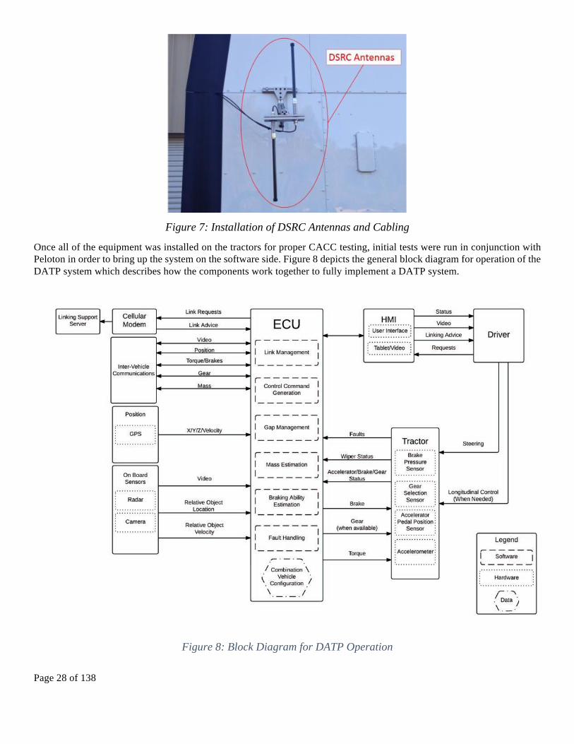
Page 28 of 138
Figure 7: Installation of DSRC Antennas and Cabling
Once all of the equipment was installed on the tractors for proper CACC testing, initial tests were run in conjunction with Peloton in order to bring up the system on the software side. Figure 8 depicts the general block diagram for operation of the DATP system which describes how the components work together to fully implement a DATP system.
Figure 8: Block Diagram for DATP Operation

Page 29 of 138
Having completed the installation, the trucks were then tested at NCAT to ensure that the system was operating safely. Figure 9 shows the two-trucks in normal DATP operation, at a separation distance of 40 feet at the NCAT facility. Several intensive brake tests were executed, and further testing was conducted to improve the control algorithm. This resulted in a high confidence level moving towards a full Type II Fuel economy test.
B.)Closed-Course Fuel Economy Testing of DATP System
After installing the Peloton platooning system onto the two Peterbilt 579’s and extensive testing on the NCAT track, the GAVLAB, along with Peloton Technology, brought the platooning trucks to the Transportation Research Center (TRC) in Ohio in August 2015. The primary goal of the fuel economy testing was to characterize the fuel economy gains that a DATP system would likely generate, evaluated in detail across a variety of factors not examined previously.
An extensive report detailing the results and conclusions is included in Appendix A. A quick summary of the results is presented in this section to provide a general overview:
For fuel economy testing of heavy vehicles, the SAE Type II Fuel Economy test was selected as the industry accepted test to determine the fuel savings obtained from implementation of a DATP system. While the SAE Type II Fuel Economy test may not accurately model a real-world drive cycle, the controlled nature of the test yields far more consistent results. The SAE Type II standard is a very rigorous testing procedure, allowing only a 2% variance within separate runs to ensure a high degree of similarity between runs.
After warming up the trucks and completing several laps on test, the fuel was measured gravimetrically and compared to the baseline tests and control truck. The results from the test are presented in the plot below:
Figure 9: Peterbilt 579 Tractors in Platoon Utilizing Peloton’s Prototype DATP System

Page 30 of 138
All testing was conducted at 65 miles per hour. The fuel economy testing yielded data that suggests that the tested DATP system provides a significant net improvement in fuel savings. The peak team fuel savings 6.96% at 30 ft, while the peak following truck fuel savings was found to be 10.24% at a following distance of 50 ft. Typical commercial operations of DATP systems is expected to have minimum allowable following distances to be in the range of 50-75 ft due to driver comfort and public acceptance. Longer following distances at 75 ft could be utilized during adverse traffic or weatherconditions and still yield fuel savings of 10.11% for the following truck and 5.59% average for the team.
Note that the trend of savings for the following truck is non-monotonic. The fuel savings at a 30 ft following distance are less than the peak savings observed at 50 ft of 10.24%. This declining trend at the closest following distances was also observed during previous testing conducted by NREL. The team consulted closely with NREL researchers in assessing results.
It is also noticeable that the following truck fuel savings does not sharply decrease as following distances increase. The lead truck does not appear to have significant fuel savings at 150 ft. Despite this, even at large following distances, the following truck’s, and therefore the team, fuel savings do appear to be significant.
One aim of this testing was to reduce or eliminate the conditions that were identified as likely contributors to the non-monotonic trend of the following truck observed in the NREL tests. In the NREL tests, parasitic loads from the radiator fan and an unrefined control of torque were identified as potential contributors to the fuel savings decline at closer followingdistances. Prior to the testing at TRC, the control algorithm of the system under test was further developed and both of these factors showed improvement without compromising the ability of the platooning controller to maintain a consistent following distance. Therefore, more investigation was needed to characterize factors that could influence fuel consumption at closer distances. Factors including air intake temperature, environmental factors (e.g., wind speed and wind direction), engine temperature, torque, and torque request rate were analyzed as to their effects on fuel savings.
The results from TRC testing showed a significant decrease in fuel consumption during DATP operations. Despite this, the following truck’s drag reduction trend experienced local maxima at a separation distance of 50 ft, in contrast to CFD modeling results suggesting that the following truck’s trend should be monotonic 5–7.
Some characteristics of the fuel savings observed indicate that further research is needed to classify the non-monotonic trend of fuel savings for the following truck at close distances. After significant data analysis following the on track testing, the team was unable to pinpoint a single cause for the deviation of the test results from the predicted fuel economy
Figure 10: Percent Fuel Saved from TRC Type II Fuel Economy Testing

Page 31 of 138
improvement from the percent drag reduction as indicated by the CFD analysis. Several possible explanations for this behavior are explored in the report presented in Appendix A. Some of the more prominent investigations are summarized below.
1. Lateral Offset Analysis
One of the benefits of using Differential Real-Time-Kinetic (D-RTK) GPS is the ability to gain extremely accurate GPS positioning solutions. Between the trucks, position differences can be accurately determined up to the centimeter range. This should, in theory, be able to provide a highly resolved view of the lateral offset between the vehicles. This is highly relevant to the investigation of the results obtained from the fuel economy testing at TRC, as one of the explanations posited by the Aerodynamic Research Group is that lateral offset negatively impacts the platoon.
Unfortunately, the compressed range message, RangeCMP was corrupted during the logging of the fuel economy test, and a full D-RTK solution was therefore not able to be resolved. Despite this, a less accurate approximation for the lateral offset was conducted; in an attempt to generally characterize what offsets occurred during the testing. The simple Best Position (BestPOS) message was then differenced in order to calculate a lateral offset. Once again, this analysis is considered in much greater depth in the TRC report in Appendix A, with a summary of the results presented below:
The decrease in standard deviation of the lateral offset as the following distance decreases, observed in Figure 10, may indicate that the driver ability to hold on offset is not affected by buffeting. Observe that the mean of the lateral offset is nonzero for all distances and from 75 ft and below the mean lateral offset is very near 0.25 ft for each. This near consistent mean across following distances may indicate that a platoon could be sensitive to even a lateral offset of less than 1 ft at closer distances.
Another important measure is the time spent above a certain threshold where the degradation of the fuel trend is exceedingly high. The plot in Figure 12 shows the amount of time spent above 1 and 2 feet lateral offsets.
Figure 11: Lateral Offset vs. Following Distance during TRC Testing

Page 32 of 138
From this data, it can be concluded that the time spent above severe offsets is relatively low when compared to the amount of time, with the highest severe offset percentage of 2.4% at separations distances less than 100 feet. Additionally, the platoon almost never experienced offsets greater than 2 feet, suggesting that a two-foot lateral offset is justified as a practical maximum. The GAVLAB intends to do a series of follow up testing with correctly logged RangeCMP messages in order to obtain a more accurate characterization of the lateral offset trends during platooning.
2. Controller Dither
Another potential culprit identified for the following truck’s diminishing gains at close separation distances was controller “dither.” During previous testing conducted by NREL, a large amount of variation in throttle control was experienced as the controller aggressively maintained the separation distance. Since then, the control algorithm was improved dramatically. During the testing at TRC, the system exhibited a large decrease in this throttle dither. For confirmation, a detailed analysis of the torque commanded was completed. A short summary of the results are provided below, where the full analysis is presented in Appendix A. Figure 13 shows the average change in torque during the test session versus the following distance.
Figure 12: Time Spent Above Selected Offsets

Page 33 of 138
The general conclusions from the analysis was that while there may be a slight increase in the amount of controller dither as the separation distance diminshed, this increase was neglible, especially when compared to the previous tests. Despite the less aggressive nature of new control algorithm at the close spacings, the error in the longitudinal spacing remained very low. This can be seen in Figure 14.
Figure 13: Average Change in Torque of the Following Truck vs. Following Distance
Figure 14: Average Error of Measured Following Distance vs. Following Distance

Page 34 of 138
From these results, it was concluded that controller dither was not a significant factor to the trend of the fuel savings performance in the following truck. For a further discussion of the average torque and relative speeds of the vehicles, please see Appendix A.
3. Engine Temperature
In previous NREL testing, another possible explanation for the following truck’s diminishing returns at close spacings was presented. During those tests, NREL identified that at close spacings, the engine fan turned on, which was not present at larger following distances or during baseline runs 4. This may be due to the decreased velocity of air in the slipstream of the lead vehicle. This decreased velocity leads to a reduction in convective heat transfer across the engine. This effect may have been exacerbated by the high ambient temperatures or other environmental factors experienced during the testing in Texas. In general, NREL determined that the engine radiator fan turned on when the coolant temperature rose between 7-8% during the testing in Texas.
During the TRC testing, the radiator fan was never engaged while the trucks were at test speed. This was true regardless of following distance, environmental conditions, or if the trucks were completing test or baseline runs. While underhood temperature and flow conditions were not a focus of the TRC testing, some data post processing was conducted in an attempt to identify potential data trends with respect to following distance. Figure 15 shows the average coolant temperature as a function of distance.
Once again, a full examination of the engine temperatures as a function of separation distance are discussed in Appendix A. From the results presented, the engine temperature did not increase as a function of the separation distance, with the following truck having overall lower temperatures than the lead truck. Additionally, the lead and following truck switched positions in the platoon for one of the test distances, and followed the truck’s trend rather than the position’s. This further solidified the argument that the engine coolant temperature was not a large contributing factor to the fuel economy trend as a function of distance.
Figure 15: Mean Engine Coolant Temperatures vs. Following Distance

Page 35 of 138
4. General Results and Conclusions
With regards to the original hypothesis, “DATP technology is near market-ready for industrial use and will provide value in specific roadway and operating conditions for heavy truck fleet operations,” the prototype DATP system demonstrated a high level of sophistication, with the control algorithm being significantly improved to provide better longitudinal control, while utilizing a lower rate of change in the torque demanded. In general, the testing at TRC helped support the overall hypothesis that DATP technology is near market ready.
In two-truck platooning, the lead truck allows the combined fuel economy trend to continue to increase at closer spacings. Since the lead truck receives a 2% benefit near 50 feet, and a larger benefit at closer following distances, it more than makes up for the decline in following truck fuel savings at those distances. It can be concluded then that for optimal two-truck platoon fuel economy performance, the platooning trucks should be spaced as close as is safely feasible. Lateral offset is a potential culprit for following truck’s trend, and thus improving lateral control could potentially be an effective means for increasing the performance of the platoon. Further research and testing is needed to confirm this new hypothesis.

Page 36 of 138
VI.V2V Wireless Communications
A. DSRC Radio Performance Test
Two Denso DSRC radio boxes (WSU-5001) were delivered to the team in the last quarter of phase I. The Software Development Kit (SDK) and documentation for WSU-5001 were sent to the team in January of 2015. These hardware and software are the same ones that are deployed on the two test trucks at NCAT. Thus, it is important to study the reliability, efficiency, and behaviors in different situations of this configuration. The team evaluated the hardware and in this phase, developed a new algorithm to mitigate the bandwidth requirements of the system.
1. Background on Real-world DSRC Radios WSU-5001 is a DSRC communication box. Like other dedicated networking devices, this type of communication boxes performs the best when working solely as communication boxes, and nothing else. Although the box has ports for CAN bus and other peripherals, they are normally used to support Basic Safety Message generation. Since the processing power of the box is limited, not all applications can run smoothly on it. Thus, it provides an option for applications to run on another computer and interface with it through Ethernet when communication is required. This is called Off-board Access. It is contrary to the On-board Access, in which case applications run on the dedicated communication box directly.
There are trade-offs when choosing between Off-board and On-board access. On-board access provides the most complete set of functionalities, with lowest latencies. In contrast, Off-board access is limited by the service daemon running on the communication boxes for what functionalities are accessible, and the Ethernet link adds extra latency. However, Off-board access provides much more flexibility for application environment, such as CPU architecture (e.g. x86/arm/powerpc) and processing power requirements.
The utilized prototype Peloton system uses Denso boxes through Off-board access. That is, an independent computer is used to run various services supporting the platooning system and it communicates with Denso radio boxes through Ethernet. Two Denso boxes are used in the system. One of the boxes is used to pass safety messages. These messages contain information on the truck’s motion states and are crucial to the safety of the platooning application. This box is used primarily with its Wave Short Message Protocol (WSMP) service. The second box is primarily used for video footage that is transmitted from the lead truck to followtruck. IP stack is used on this box.
After some investigation, the team decided to only test the WSMP stack, due to two reasons: 1) the WSMP stack is crucial in the platooning application as well as other safety applications; 2) the team was not able to configure different parameters (e.g. data rate) for IP stack using the commands provided by Denso.
This left two choices: On-board WSMP and Off-board WSMP. Since Off-board WSMP is used by the platooning system for safety messages, it is a reasonable choice for measuring as close to the real using scenario as possible. However, GPS timing available through the Off-board service is not precise enough. It only gives 0.01 second’s precision, while latency on wireless transmission can be lower than 1 millisecond. On-board access, on the other hand, allows the use of the system time on the Denso box, which is synchronized with GPS time automatically. This measurement is then precise enough for measuring wireless latencies. As a result, the best way to evaluate the Denso radio boxes is to run a WSMP stack with On-board access.
2. DSRC Testing Plan There are many parameters that affect wireless communication. Different parameter settings result in different performance for different hardware and use-cases. To understand how DSRC would perform in different situations and to find optimal parameter settings for different situations, the following parameters were examined in the tests:

Page 37 of 138
• Channel: The channel specifies the wireless channel that the test program should use. There are seven 10 MHz channels and two 20 MHz channels defined in DSRC and usable on Denso radio.
• Data Rate: Data Rate specifies how many bits of data the Media Access Control layer and Physical layer can encode into electro-magnetic signals, per second. It does not necessarily mean how much the data applications send out per second, but rather implies the capability of lower layers. Higher data rates mean more data can be sent per unit time, but also results in higher signal-to-noise ratio, causing high packet loss when the receiving device is not in a good position. Thus, choosing the proper data rate is important for ensuring reliability as well as efficiency of the wireless communications. On 10 MHz channels, selectable data rates include 3, 4.5, 6, 9, 12, 18, 24, and 27 Mbps, while on 20 MHz channels, selectable data rates are 6, 9, 12, 18, 24, 36, 48, and 54 Mbps.
• Message Rate: Message Rate specifies how frequently the test program should send a message. High message rates might cause congestion or be limited by radio capability, while low rates sometimes are not sufficient for some applications.
• Message Size: Message Size specifies the size of each message that the test program should send out. • Antenna: Antenna specifies which one of the two antennas to use. When the trucks are positioned in a straight
line, this may not matter. Since the antennas are mounted on the sides of the truck, one of the antennas may get blocked as the truck is turning. It is important to know how well the antenna can perform when the trucks are in different positions. An alternative to always using one of the two antennas is to use both antennas alternately. However, when one of the antennas is blocked, this might cause half of the messages to be lost. A workaround is to send each message twice, so that each message is sent through both antennas. This approach provides reliability through redundancy, but might cause unnecessary wireless congestion. Thus, it is important to study different situations and analyze the best antenna configuration for each situation to limit the congestion when reliability is sufficient in a single-antenna setup.
Different values for each of these parameters were tested for each position configuration. During dynamic testing, position configuration can mean different positions on the test track, such as straight line and cornering. For static testing, position configurations can vary based on the following: separation distance of the trucks, including trailers or not, or whether the trucks are turning or not.
3. Design and Implementation of the Test Program
The test program runs in either TX (transmitting) or RX (receiving) mode. Normally the TX mode runs on the lead truck, while the RX mode runs on the following truck. In TX mode the test program broadcasts messages through the WSMP stack according to specified parameters, and logs a timestamp and the sequence number for each message when it is being sent out. In RX mode, the test program listens on the channel with a specified private system identifier (PSID), and logs a timestamp whenever it receives a message, along with its sequence number. (In RX mode, the Denso radio chooses its receiving antenna automatically and is not configurable.) By comparing the timestamp from TX logs and RX logs for each sequence number the latency of each message can be calculated. This latency would include various software-introduced delay on both devices, including user-space API and kernel-space processing, as well as the wireless propagation time.
To carry out the DSRC testing plan described above a test program was developed to support different parameter settings. Below is the output of help message of the test program, which gives an overview on available flags for setting the parameters:
Usage: ./tester < --tx | --rx > [options]
General Options:
--help : display this help
--log-file <filename> : specify path to log file | default=<STDOUT>
--tx : start as TX
--rx : start as RX
--gps <filename> : specify path to log file for GPS location data.

Page 38 of 138
If this flag is not present, GPS logging is disabled.
--psid <psid> : specify WSM PSID to register | default=80 (0x50)
--channel <channel> : specify channel to send/receive WSMs | default=174
: 10 MHz channels: 172 174 176 178 180 182 184
: 20 MHz channels: 175 181
--antenna <antenna> : specify antenna to send WSMs | default=0
has to be one of 0, 1, or 2
0: alternating (TX) / diversity (RX)
1: always use antenna 1
2: always use antenna 2
TX Specific Options:
--duplicate : send each message twice
--power <power> : specify power to send WSMs | default=20
--priority <priority> : specify priority to send WSMs | default=2
--msg-rate <rate> : specify # of WSMs to send per second | default=0
0 means sending as fast as possible
--msg-size <size> : specify # of bytes of each WSM | default=1399 (max)
--data-rate <rate> : specify MAC data rate (Mbps) for WSMs | default=6 (max)
10MHz CH rates: 3 4.5 6 9 12 18 24 27
20MHz CH rates: 6 9 12 18 24 36 48 54
Among these parameters, most can be configured through Denso provided APIs. For the message rate, a custom algorithm design was required to ensure the processing delay does not interfere with the message rate. The algorithm can be summarized in the following steps:
1. Based on message rate, calculate the expected interval, d0, between adjacent messages. This interval is the duration passed from the moment a message should be sent out, until the moment the next message should be sent. It is calculated by dividing 1 second by the message rate. For example, for 10 Hz message rate, d0 == 0.1 seconds.
2. Initialize the wireless radio service. Store current timestamp to t0. Initialize the message counter, c, to be 1. 3. Calculate expected timestamp, t1, to send the message: t1 = d0 * c + t0. 4. Take current timestamp t2. If t2 > t1, sleep for t2 – t1, and take current timestamp again, store in t2; Otherwise,
simply carry on to step 5. 5. Send the message, and t2 would be the timestamp for the moment when the message is sent. 6. Increase the message counter c, and go back to step 3.
Through this algorithm, the interference on timing from the processing delay is minimized, so that the achieved message rate is as close to the set value as possible (when the set value does not exceed system’s capability). Also, the logged timestamps of each message are as accurate as possible.

Page 39 of 138
4. Static Testing Results
Several static DSRC tests were carried out using the two test trucks at the NCAT facility. Channel 174 was used for all tests. Other parameters were configured iteratively through the following possible values:
•! Antenna: alternate with duplication (0d), alternate (0), passenger side (1), driver side (2)] •! Data Rate (Mbps): 3, 4.5, 6, 12, 27 •! Message Size (bytes): 4, 256, 1399 •! Message Rate (Hz): 1, 50, 100, unlimited (0)
Each configuration, for example: antenna 1 / data rate 3 / message size 1399 / message rate 10, is considered a test case. For each test case, the test program runs for either 30 or 60 seconds based on the message rate setting. A set of tests based on such configurations is called a test suite. In this case, each test suite contains 240 test cases.
The test suite ran for several different static position configurations. Some representative ones are presented in this section.
i.) Close Distance with Building on One Side without Trailers
In this position configuration, the trailers were detached from the tractor. The two truck tractors were placed close to each other, positioned in a straight line. The distance between the antennas on both trucks was 33 feet. A building that was approximately as tall as the trucks was on the left side (driver-side) of the two trucks. The trucks were 2 feet from the building and the building can reflect signals. The weather was sunny at approximately 75 degrees. Figure 16 demonstrates this configuration.
Figure 17 shows the latency measurements for all tested configurations. Each column is an antenna configuration. Each row has one message rate configuration. Different messages are represented with different line and marker styles. X-axes are data rate settings, while Y-axes are message delivery ratio.
Figure 16: Close distance with building configuration diagram

Page 40 of 138
There are several interesting trends shown in the figure:
1.! Even though the trucks were close to each other, the package delivery ratio tends to decrease when data rate increases. These changes seem to happen when above 12 Mbps.
2.! Using the passenger side antenna (Antenna 1) results in better delivery ratio than using driver side antenna (Antenna 2). This might be due to the reflections from the building on the driver side which causes signal collisions.
3.! The alternating with duplication antenna configuration is as good as, or better than, using the passenger side antenna.
ii.) Large Separation Distance in an Open Area without Trailers
In this configuration, the two trucks were positioned in a straight line in an open area where no buildings were close. The trailers were detached from the tractors. Antennas on both trucks were 265 feet from each other. Several other trucks wereon the right side (passenger side) of the trucks but were discrete and without tall trailers that can reflect signals. The weather was sunny at approximately 70 degrees. Figure 18 shows this configuration.
Figure 17: Delivery Ratio (Close Distance with Building on One Side without Trailers)

Page 41 of 138
Figure 19 shows the delivery ratio for this configuration. As shown, in all parameters, the packet delivery ratio was close to 100%. This is true even for high data rates. In general, DSRC performance degrades as the distance between the antennas is increased. Despite this general trend for all DSRC systems, even though the open area tests were conducted at a larger distance than the previous tests the delivery ratio was still higher. This suggests that an open environment is extremely important to the performance of a DSRC system.
Figure 18: Schematic for Open Area Testing
Figure 19: Delivery Ratio (Large Separation Distance in Open Area without Trailers)

Page 42 of 138
iii.) Large Separation Distance on Uphill and Downhill
In this position configuration, the two trucks were still detached from trailers. They were also positioned in a straight line. Antenna separation distance was also 265 feet. The primary difference from the previous case is that the trucks were placed on the right lane of an unused road, where a small hill was between the two trucks. The lead truck was positioned on the downhill portion of the hill, while the following truck was positioned on the uphill portion. This situation causes the two trucks to become angled; hence the antennas are no longer parallel. Due to the mechanism through which wireless propagation works, this situation introduces degradation in wireless performance. The weather was initially cloudy thentransitioned to sunny, with a temperature of approximately 70 degrees. Figure 20 shows this configuration.
Figure 21 shows the delivery ratio for this configuration. Although the configuration was still an open area, the delivery ratio drops significantly at higher data rates, due to the hill that causes the angular change between the antennas. The passenger side (right side) antenna performed slightly better than the driver side (left side) antenna. One possible reason is that the trucks were in the right lane, and thus were closer to trees on the right side of the trucks, which improves performance by providing signal reflection. However, it is not certain if this is consistently true, since the terrain of trees is more complex.
Figure 20: Schematic for Large Separation Hill Testing

Page 43 of 138
iv.) Large Separation Distance with Lead Truck Turning
In this position configuration, both trucks had the trailers attached. They were positioned 200 feet from each other (antenna-to-antenna), located on the left lane of a plain road. Unlike the previous static tests where the trucks were in a straight line, in this configuration the lead truck was turning left (driver side). Since the tractor of the lead truck was angled to the left, the antenna on the passenger side was entirely blocked by the trailer of the lead truck. This is to simulate the situation where trucks are going through a curve and one of the antennas may be blocked. In the static setups, the lead truck is turning somewhat sharper than a truck would normally turn on highway. Figure 22 shows this configuration.
Figure 21: Large Separation Distance with Uphill and Downhill

Page 44 of 138
Figure 23 shows the delivery ratio for this position configuration. Each column represents an antenna configuration. “Antenna 0” means using both antenna alternately; “Antenna 1” is the right-side (passenger side) antenna; “Antenna 2” is the left-side (driver side) antenna.
Figure 22: Schematic for Lead Truck Turning Configuration
Figure 23: Delivery Ratio When Lead Truck Is Turning Left

Page 45 of 138
As shown in the figure, the left-side antenna constantly shows a delivery ratio of or close to 100%, while the right-side antenna starts to fail to deliver a portion of messages when the data rate goes beyond 12 Mbps, and the delivery ratio reaches 0 at 24 Mbps. “Antenna 0” (alternated transmitting) verifies this by showing 50% delivery ratio starting at 24 Mbps.As noted above, the position configuration simulates the situation when the trucks are turning, but these turn angles exceed typical highway driving. Nevertheless, these results reflect the networking reliability when trucks are turning at these specific angles. The inside antenna continues working well throughout the curve, while the outside antenna sees some packet loss. This validates through real-world, device based experiments, that using two antennas on alternate sides is necessary for operating vehicles in environments with sharp turn angles.
The team continues to see high latency values occasionally, but the ultra-high latency situation is very rare. Throughout most of normal operation the latency is within 10 milliseconds. At lower data rates, the latency tends to be high. This is because at lower data rates, it takes more time to encode the same data, which adds to the overall latency. The latency results are shown in Figure 24.
Figure 24: Latencies When Lead Truck Is Turning Left

Page 46 of 138
5. Dynamic Tests from NCAT Track
The team conducted several different dynamic tests. The entire dynamic test suite consists of 162 individual test cases. Each test case has a different combination of parameters:
Data Rate (Mbps): 3, 4.5, 6, 12, 18 24 Message Size (bytes): 50, 256, 1399 Message Rate (Hz): 10, 20, 100 Antenna: inside, outside, alternate
The trucks operate at speeds of 45 – 55 mph on the 1.7 mile long NCAT track. This means that each test case was run for 111 – 136 seconds. To make sure each test case could safely cover the entire track, the team asked the drivers to try to maintain the speed above 47 mph, and set the run-time for each test case to be 135 seconds.
The parameter values were chosen to represent real operating environments:
1. Data rate: starts at 3 Mbps, which is the lowest on 10 MHz channel, and goes up to 24 Mbps, with lower rates covered at finer increments than higher rates. This is because in broadcast scenarios, which is the case for BSMs, higher rates will result in very high packet loss, thus are unlikely to be useful for the platooning application.
2. Message size: 50 bytes is about the size of smallest BSM; 256 bytes is selected as a representative size of the BSMs in a platooning application, including the custom structure tailed in the end; 1399 bytes is the maximum allowable WSM on Denso’s DSRC device.
3. Message Rate: 10 Hz is the rate that platooning BSMs are sent; 20 Hz is the rate of actual WSMs when duplicate is enabled; 100 Hz allows us to observe DSRC reliability when the application is sending much faster.
Unlike static tests, dynamic test results need to be shown in the context of location of trucks. As a result, it is infeasible to show data in an aggregated form as in static tests. The team plotted delivery ratio figures using a scatter plot in context of GPS locations. Therefore, each test case generates one figure. Instead of presenting all 162 figures, only some representative cases are shown.
All figures are scatter plots. Each red point represents one instance of packet loss, and each blue point represents a packet that is successfully delivered. All points’ X-Y values are representative of GPS coordinates corresponding to the location on the track. Since the points are very densely distributed, to make the figure more readable, all red points (packet losses) are added with 6 meters offset on both X-axis and Y-axis.

Page 47 of 138
v.) Group 1: Varied Antenna Configuration
The first group of representative test cases are shown above. The three test cases share the same data rate (lowest at 3 Mbps), message size (largest at 1399 bytes), and message rate (20 Hz). The only difference was the antenna configuration. As one might expect, the outside antennas perform poorly when going through curves. As shown in the figure, the two straight lines are nearly all blue, meaning the majority of messages were delivered, while the two curves are composed of red points representing packet losses. This is most likely because the outside antennas were blocked by the trailer of the lead truck. What is unexpected, but still explainable, is that the inside antennas, while performing very well on curves, have lots of packet loss on the two straight line portions of the track. This may be due to the reflections from the center area of the track, which is heavily wooded. If so, these reflections cause multipath signals, which seemed to be affecting the transmission. On the curves, the reflections occur much less often than in the straight line travel, which signifies that the inside antenna performs well.
Figure 25: Received and unreceived packets during testing around the NCAT facility test track for inside, outside, and alternate configuration of antennas.

Page 48 of 138
vi.) Group 2: Varied Message Size
The second group of representative test cases are shown above. They still used the lowest data rate (3 Mbps), the message rate of 10 Hz, and usage of outside antennas. The varied parameter was the message size of WSMs. As shown in the figure, 50 byte messages at 3 Mbps were mostly delivered even using the outside antennas. Even during the curves, most consecutive messages were still delivered. However, while the message size increases, the packet loss becomes worse and fewer consecutive messages were delivered during curves.
Figure 26: Received and unreceived packets during testing around the NCAT facility test track for 50, 256, and 1399 byte message sizes

Page 49 of 138
vii.) Group 3: Varied Data Rate
Figure 27: Received and unreceived packets during testing around the NCAT facility test track for varied data rates of: 3Hz, 4.5Hz, 6Hz, 12Hz, 18Hz, and 24 Hz

Page 50 of 138
The third group of representative test cases are shown above. These tests use a 256 byte message size, 20 Hz message rate, and outside antennas. The varied parameter is the MAC layer data rate. As shown in the figure, with a 256 byte message size, even at the lowest rate, the packet loss of outside antennas is significant during the curves. The delivery ratio becomes worse when data rates increase. As the data rates are increased to 20 Mbps and higher, messages are often not delivered even on the straights.
While not shown here, it is worth mentioning that the inside antennas showed good performance even at high data rates for a message size of 256 bytes. The inside antennas often still lossed packets on the straight track when compared to on the curves. Delivery ratio for the inside antennas was also worse at the higher data rates, but the overall performance is much better than outside antennas at higher data rates.
viii. Aggregated Results for Dynamic Tests
While the individual plots provide details on how each location of the track affects the results, it does not give a high-level view on how different parameters affect the delivery ratio. Thus, the team further analyzed the results by aggregating the delivery ratio results from different runs. The results are divided into two sub-groups. As shown in Figure 28, white straight lines and red curves form the two groups.
In addition to the aggregated results, a new type of metric is also introduced: pairwise delivery ratio. It is similar to the normal delivery ratio, except that it represents the ratio of the messages delivered from either of a pair of antennas to the total pairs of messages sent. In pairwise delivery ratio, delivery of any one of a pair of duplicate messages indicates successful transmission of both. This metric (the pairwise delivery ratio) is only applicable when the “alternate” antenna configuration is used. Since each message is transmitted twice, success of any of the two transmissions in a pair is sufficient for successful delivery of the message.
Figure 28: Test Track Partition

Page 51 of 138
Figure 29 shows pairwise delivery ratios when the antennas were set to alternating mode. Since the pairwise delivery ratio takes two consecutive transmissions (one from inside antenna and the other from outside antenna) for each message, the
Figure 29: Delivery Ratio From Dynamic Tests: Alternate Antenna

Page 52 of 138
advantages for antennas during curves or straight lines are eliminated. Instead, the pairwise delivery ratio is determined by the best performing antenna at the moment. As shown in the figure, apart from the previously stated phenomenon that higher data rates result in lower delivery ratio, one can also see that delivery ratio is actually better during the curves than thestraight lines by comparing the two columns in the figure. The team believes this is because during curves, the signals ofthe inside antennas were less affected by the lead truck trailer or nearby terrain than that of either antenna on the straight lines.
Taking a closer look at how each of the antennas performs, Figure 30 shows the delivery ratios when both trucks used theside antennas. The general trends found in the figure are consistent with Figure 29. Specifically, for this particular test track configuration,
•! Inside antenna generally performs better at curves than on straight lines, especially with larger message sizes.
•! Outside antenna performs better on straight lines than at curves with larger message sizes at lower data rates.
•! Inside antenna performs better than outside antenna at curves in all cases, as expected.
The outside antenna performed better than the inside antenna on straight lines in a vast majority of the cases, and the difference is much larger at lower data rates.
Figure 30: Delivery ratio from dynamic tests on test track: side antennas

Page 53 of 138
ix. Conclusions
With these results from the experiments at the NCAT track, the Auburn wireless communications research team has concluded the following about DSRC inter-vehicle communications performance for tractor trailers pairs, at least regarding the effects of the curvature in the specific setting of the NCAT track:
• Being blocked by the truck trailer affects the outside antennas’ performance significantly, especially when the message size is large.
• Performance of the left (driver side) antenna depends on the effects of reflections from the terrain or other nearby vehicles.
• Larger messages worsen the delivery ratio (a factor not specific to DSRC). • Higher data rates normally result in lower delivery ratio (a factor not specific to DSRC)
B. Interframe Compression Transmission Layer
One of the important findings from the performance tests was that, by utilizing both antennas alternately and using lower data rates, DSRC communication is generally very reliable and can support platooning applications very well.
Looking beyond, the Auburn wireless communications research team believes that it is also important to think about scalability issues. When DSRC is fully deployed in the future, the DSRC networking will face more pressure from various applications. This presents interesting research topics that the team believes are worth looking into to ensure viability in the future. From this aspect, the team has looked into scalability analysis and possibilities of reducing bandwidth for future vehicular applications.
1. Problem Analysis – An Extreme Case Study
In many cases for 802.11 communication, channel congestion is a key issue that affects performance, and needs to be relieved through various techniques. Previous reports have shown that, by utilizing both antennas and choosing lower data rates, DSRC networking performance is very reliable, approaching 100% packet delivery ratio. However, when looking at scalability aspects of the system, and aiming to solve issues for the future, it is useful to analyze extreme conditions. While not necessarily relevant to near-term deployment, a scenario was devised for a dense communications environment in a highway setting when a high percentage of vehicles are equipped.
Here, a simple analysis of an extremely heavy use case is presented. The following are some assumptions made for the analysis:
• Average following distance: 10 meters. In the previous phase, the aerodynamic analysis predicted that fuel saving is significant when following distance is below 40 feet (about 13.3 meters). Thus, as an extreme example, 10 meter inter-vehicle distance is used.
• Platooning message size: 150 bytes. SAE J2735 defines Basic Safety Message (BSM), which includes various vehicle messages that are helpful to vehicular safety applications. It has approximately 50 bytes of data which are required data elements that appear in every transmission. After the required portion, vendors can attach proprietary data structures. The team assumes 100 bytes for this portion, in order to support applications such as platooning. Including the required portion of BSM, a DSRC message is assumed to be 150 bytes.
• Total lanes: 10. Some busy highways may have 5 lanes per direction at busy segments, especially near an interchange. An example is an area1 near the Atlanta airport in the US, where Interstate 285 has 5 lanes per direction, with other roads or highways nearby. Thus, the team assumes 10 lanes in analysis for heavy-use cases.
1 https://www.google.com/maps/@33.6205067,-84.4576489,1936m/data=!3m1!1e3

Page 54 of 138
• Interference range: 400 meters. Interference range is larger than effective communication range. With DSRC radios designed to reach several hundred meters, 400 meters’ interference range is used here.
• MAC layer data rate: 6 Mbps. Generally speaking, higher data rate results in lower the signal-to-noise ratio under the same environment. Lower signal-to-noise causes higher packet error rate. This affects reliability of transmission. The team has shown that the delivery ratio may drop significantly above 6 Mbps. Safety applications like platooning require high reliability, so it is assumed that the 6 Mbps is selected all the time.
• Platooning message rate: 20 Hz. This assumes dual-antenna configuration and alternate mode. In other words, at 20 Hz, the effective message rate is 10 Hz, or one message sent twice every 100 milliseconds. This results in about 3 meters in distance at a speed of 110 km/h.
Consider a target vehicle on a busy segment of a highway. With 400 meters of interference range, the vehicle is interfered by vehicles within 400 meters’ radius, which means an 800 meters long segment on the highway. Assuming full market penetration and full road utilization, linear vehicle density is 1 vehicle/10 (meters×lane) = 0.1 vehicle/meter/lane. With 10 lanes in total for both directions, there are 800 meters×10 lanes×0.1 vehicle/meter/lane = 800 vehicles within the interference range. At 20 Hz per vehicle, messages are being sent at 800 vehicles × 20 Hz/vehicle = 16,000 Hz within the interference range. Multiplying this by the message size 150 bytes, the total bandwidth usage can be calculated as 16,000 Hz × 150 bytes = 2.4 MBps, or 19.2 Mbps.
In contrast, the MAC layer data rate 6 Mbps, which is much smaller than the requirement in this extreme situation. Furthermore, due to the channel switching strategy defined in IEEE 1609.4, only half of the channel time can be used. Along with MAC layer overheads, such as the contention window and various spacing in CSMA, management frames and control frames. The available bandwidth available for upper layers is further reduced.
Although the analysis is based on an extreme situation, it presents an interesting research topic, which is the DSRC congestion problem. The congestion problem implies that DSRC applications may face technical challenges in extreme situations.
There have been various congestion control algorithms proposed and standardized (such as congestion control in SAE J2945.1) to relieve the congestion, but all sacrifice reduced message frequency and/or transmitting range. The Auburn wireless communications research team believes that, as a defense measure before the congestion control, it is worth looking into reducing bandwidth usage of DSRC applications, aimed at preventing congestion from happening rather than mitigating it after it occurs.
Based on the stakeholder engagement and high-level requirements development in other portions of this project, it should also be noted that the operational parameters of platooning can be adjusted due to many conditions, such as weather and traffic density. Any performance degradation in the communications channel, due to congestion and other factors, could be detected by a platooning system before it reaches a critical stage such that the inter-vehicle gap could be widened or the platoon dissolved until conditions improve. Decisions to approve a new platoon or dissolve an existing platoon are made at a much lower frequency than that which is required by BSMs. Unlike active safety systems relying on V2X, platooning systems are not required to be “always on” and thus can be expected to adapt to degradation of the channel.
2. Design of the Algorithm
In phase I, the team explored possibilities of using differential data to reduce bandwidth usage in vehicular networks. The team did not finish designing this system because j2735 was already compact, and the necessary components for supporting differential data on a field by field basis for each message type were too complex. This led to the conclusion that the implementation and development cost, as well as the cost caused by the increase in the system complexity, would outweigh the benefit.
In this phase, the team revisited the differential concept. A simplified method called Interframe Compression Transmission Layer, or ICTL was devopled. The ICTL is a separate lower layer that operates on differential data and uses an arbitrary data structure in the vehicular network.
Inter-frame compression is a fundamental concept behind many video compression algorithms such as MPEG-2 and H.264. Since consecutive frames in a video are normally very similar, encoding them individually results in low entropy, which is a waste of bandwidth. With inter-frame compression, video codecs encode complete frames (Intra-frames, or I-frames)

Page 55 of 138
infrequently. Between these complete frames, only changing parts are encoded (Predictive-frames or P-frames, and Bidirectional-frames, or B-frames). These frames are packed into Group of Pictures (GOP) structures. A typical GOP structure is IBBPBBP. . .PBBI. Since B-frames and P-frames are much smaller than I-frames, the complete video stream uses much less bandwidth.
Messages in a vehicular network can benefit from inter-frame compression as well. An important attribute of video streams which allows for inter-frame compression is that consecutive frames are very similar, with only slight changes in parts of the frame. This is true for messages in vehicular environments as well. Within a small portion of the road, e.g. 60 meters, or roughly 2 seconds headway at 110 km/h, many dynamic attributes of the vehicle, such as steering, yaw rate, and speed, are mostly the same, as long as the vehicle is not doing a significant maneuver. Even when they change, they typically change gradually, which results in only a small number of flipped bits in binary form.
In traditional DSRC, an application constructs a SAE J2735 message, and directly encapsulates it in a WSM and sends the message through 802.11p using WSMP. With ICTL, the message is either sent as it is, or converted to a smaller byte stream containing changes from a previous complete message before being sent out. ICTL takes care of the compression and decompression, and applications see the same message identical to the original.
To support this, two types of frames are introduced:
• Key Frame (KF). A KF is similar to an I-frame in video compression. It contains the complete message being sent. A KF does not require any extra information to decode.
• Differential Frame (DF). A DF only carries the differences from a previously sent KF. Decoding the original message from a DF requires the KF that it refers to as well.
To separate DF from KF, and to identify each message, ICTL uses a 4-byte header. The following table shows the layout of an ICTL packet
Reserved Frame Type Compression Options Frame ID Payload 4 bits 4 bits 8 bits 16 bits Variable length
Zooming out to a broader scope, a typical message with all headers has a layout shown in following table:
MAC Header (802.11) WSM Header ICTL Header Payload 28 bytes 5-20 bytes 4 bytes Variable length
The Reserved field is held in reserve should a newer version of ICTL be developed. For now it should always be set to 0b0000. Frame Type indicates whether the packet contains a KF (0b0001) or a DF (0b0010). Compression options carries information about compression algorithms applied to the payload. Frame ID is an increasing unsigned integer that wraps at boundaries. It is used to identify frames sent from the same source. For a KF, it is the ID of the actual message. For a DF, it is the ID of the KF that it refers to. Payload is the actual complete message (KF) or differential message (DF). Since the WSM header already has a field for payload length, and ICTL header has a fixed width of 4 bytes, the length of ICTL payload can be easily inferred, thus it does not require an extra length field.
Compressing vehicular messages needs to be lossless. As a result, video compression techniques such as prediction cannot be used. Instead, a simpler approach using Exclusive Or (XOR) is proposed to encode differential messages in a DF.
Given a previously transmitted KF, whose payload is
, where b0i represents one bit (zero based index) of the payload p0, and a new message
a field for payload length, and ICTL header has a fixed width of 4 bytes, the length of ICTL
payload can be easily inferred, thus does not require an extra length field.
Di↵erential Encoding
Compressing vehicular messages needs to be lossless. As a result, video compression
techniques such as prediction cannot be used. Instead, a simpler approach using Exclusive
Or (XOR) is proposed to encode di↵erential messages in a DF.
Given a previously transmitted KF, whose payload is
p0 = b00, b01, b
02, b
03, b
04, b
05, . . . , b
0n�2, b
0n�1 (5.1)
, where b0i represents one bit (zero based index) of the payload p0, and a new message
p1 = b10, b11, b
12, b
13, b
14, b
15, . . . , b
1n�2, b
1n�1 (5.2)
, where b1i represents one bit (zero based index) of the payload p1, then the payload of DF,
or in other words, the di↵erential message d0,1 between p0 and p1, can be produced as
d0,1 = b00 � b10, b01 � b11, b
02 � b12, b
03 � b13, b
04 � b14, b
05 � b15, . . . , b
0n�2 � b1n�2, b
0n�1 � b1n�1 (5.3)
, where � is XOR operator1.
Since the messages that are sent within a short time window have very similar content,
the majority bits in the di↵erential message should be zero. Such message has low entropy,
and can be e�ciently compressed using a general purpose compression algorithm.
1When implementing in a programming language, this can be done by using bitwise XOR operator(normally written as )̂, and computed 8 bits at a time.
29

Page 56 of 138
, where b1i represents one bit (zero based index) of the payload p1, then the payload of DF, or in other words, the differential message d0,1 between p0 and p1, can be produced as
, where ⊕ is XOR operator1.
Since the messages that are sent within a short time window have very similar content, the majority of bits in the differential message should be zero. The message therefore has low entropy, and can be efficiently compressed using a general purpose compression algorithm.
ICTL is performed per application rather than per link. Since WSMP already handles multiplexing through PSID, ICTL uses PSID to separate different types of data. When ICTL receives a request to transmit a message from the upper layer for a given PSID, it first determines whether the message should be transmitted using KF or DF. This depends on a preset scheme that describes how many DFs can be sent between two adjacent KFs. For KF, the message is compressed, and prepended with an ICTL header. The header indicates that it is a KF, and provides the increasing unsigned integer to identify the message. For DF, the differential message is first calculated, then compressed and prepended with the ICTL header. The header indicates that it is a DF, and refers to ID of the KF that the DF is produced from. Normally, it is the most recently sent KF, but it can also be older KFs as well, depending on the networking condition when the KF was sent. If the network condition was bad when the most recently sent KF was transmitted, it may not have been successfully received by many vehicles nearby. In this case, ICTL would choose a previously sent KF to base on. Decoding is basically the reverse operation of encoding. Since the sender may choose to send a differential message based on an older message, a list of recently received KF needs to be maintained.
For analysis and experimental purposes, the concept of ICTL Cycle, and Cycle Length (CL) is introduced here:
• ICTL Cycle is defined as a sequence of ICTL frames, starting with a KF, followed by a number of DFs, given that the last DF, i.e., the end of cycle, is either the last frame of transmission, or followed immediately by a KF, which marks the start of next cycle. In the case of this study where ICTL always pick the most recently transmitted KF as reference frame for DFs, an ICTL Cycle can also be defined as a sequence of messages including exactly one KF and all the DFs that use this KF as reference frame;
• CL is defined as the number of messages included in an ICTL Cycle. For example, in an ICTL strategy that always sends 3 DFs after each KF before sending a new KF, the CL is always 4. CL can be a predefined fixed value, in which case it is a configurable parameter, or it can dynamically change according to an internal model in the ICTL implementation, in which case CL is merely an observed value driven by the ICTL implementation.
3. Implementation and Experimental Setup
The ICTL algorithm was implemented in the Go programming language. This language was chosen due to its balance between safety, development efficiency, and performance. Designed as a system language, Go has well designed support for system software, such as first-class concurrency, well-designed networking APIs and system call interfaces, and cross-compiling tools. These features benefit the development of ICTL, resulting in stability and high performance. Despite these advantages, Go provides less control over the memory management of the applications compared to other system languages such as C/C++. The garbage collection takes care of reclaiming memory no longer used, so a straightforward way to code in Go is to allocate new objects whenever needed, and let the garbage collection handle freeing the memory. This approach works in most cases. For ICTL’s use case, however, packets are generated and consumed at a very high rate, which results in byte buffers of the same size allocated and deallocated frequently. This allocation and deallocation increases the processing burden and is inefficient. In ICTL, a buffer pool is utilized for reusing existing byte buffers, using the free- list data structure. In addition, the buffer pool implements a thread-safe reference counting, similar to std::shared ptr in C++, in order to allow multiple components share the same object, and reuse objects at precisely the time when they are not needed.
ICTL is implemented as a library package that encapsulates the details of encoding and decoding behind a simple interface ictl.Endpoint, which represents an ICTL endpoint for encodings and decodings. An object of ictl.Endpoint can be created using a configuration object that specifies the behaviors of the ICTL algorithm. The endpoint has methods for encoding and decoding messages. Each of such methods accepts a context parameter, which is used to differentiate
a field for payload length, and ICTL header has a fixed width of 4 bytes, the length of ICTL
payload can be easily inferred, thus does not require an extra length field.
Di↵erential Encoding
Compressing vehicular messages needs to be lossless. As a result, video compression
techniques such as prediction cannot be used. Instead, a simpler approach using Exclusive
Or (XOR) is proposed to encode di↵erential messages in a DF.
Given a previously transmitted KF, whose payload is
p0 = b00, b01, b
02, b
03, b
04, b
05, . . . , b
0n�2, b
0n�1 (5.1)
, where b0i represents one bit (zero based index) of the payload p0, and a new message
p1 = b10, b11, b
12, b
13, b
14, b
15, . . . , b
1n�2, b
1n�1 (5.2)
, where b1i represents one bit (zero based index) of the payload p1, then the payload of DF,
or in other words, the di↵erential message d0,1 between p0 and p1, can be produced as
d0,1 = b00 � b10, b01 � b11, b
02 � b12, b
03 � b13, b
04 � b14, b
05 � b15, . . . , b
0n�2 � b1n�2, b
0n�1 � b1n�1 (5.3)
, where � is XOR operator1.
Since the messages that are sent within a short time window have very similar content,
the majority bits in the di↵erential message should be zero. Such message has low entropy,
and can be e�ciently compressed using a general purpose compression algorithm.
1When implementing in a programming language, this can be done by using bitwise XOR operator(normally written as )̂, and computed 8 bits at a time.
29

Page 57 of 138
different streams of data. In the case of DSRC, a combination of MAC address and PSID is a good choice of context. The endpoint allocates one encoder/decoder for each context, and maintains the separation between different data streams.
To test the performance of ICTL, the team developed a wireless networking emulation platform, which replaces the MAC layer and physical layer of IEEE 802.11 networking stack with a real-time CSMA/CA model. The emulator is designed to facilitate running real-world code. Everything above MAC layer assumes a real wireless device, and process real network frames. The concept was to develop research projects that are not only reproducible, but also more directly beneficial to real-world applications.
The team used data traces from platooning tests to study the ICTL algorithm and to improve its performance. To utilize such trace files, a software component was written, called truck-playback, to replay events from one vehicle. The trace files includes many events, such as GPS location, DSRC message transmission and reception, various events from each vehicle’s CAN bus, e.g. radar measurements. For the purpose of studying ICTL, two events are relevant:
• GPS location events, which are needed to update emulated locations of the truck in Squirrel; • DSRC transmission events, which indicate when to send a DSRC message and what particular data should each
DSRC message carry.
truck-playback reads the two types of events from a logged trace file and replays these events in emulation. The GPS location events are converted to gRPC requests, and sent to the emulator to update the current emulated position of the node. The DSRC events drives the truck-playback to send WSMs over DSRC at predefined time points, using traditional method, or encoded with ICTL. The content of a WSM is determined by the event content, which includes values of each data field. Sending exactly the same information as trace files is important because the content of messages and how fast the content changes affect how well ICTL compresses the messages.
Each event from the trace file is tagged with a timestamp. truck-playback synchronizes the timeline so that a time point from wall-clock during emulation is aligned with a time point from trace file’s time when the tests were conducted in the real world. In other words, a fixed offset is set between the playback’s timeline and the trace file’s timeline. When truck-playback replays an event, it first calculates a deadline based on the timeline offset. In most cases, the deadline is after current wall-clock time. A difference is calculated between the two, and truck-playback waits for such time duration by calling sleep() before actually replaying the event. This ensures that the events happen at exactly the same relative times. For example, DSRC messages are sent at the same frequency as the trace file dictates. When many nodes are emulated on the same computer, occasionally, the deadline may have already passed by the time it is calculated. In this case, this particular event is sent immediately (without calling sleep(), but is not able to meet the deadline when replayed. If too many events cannot meet the deadline, the results would not be authentic. As a result, truck-playback logs such incidents to be examined afterwards.
The truck-playback uses the WSMP implementation from Phase I, which uses system call interfaces to pass messages into or read messages from the Logical Link Control (LLC) layer in the kernel. The messages are then handled by the emulator and delivered to other nodes based on the CSMA/CA model.
When truck-playback replays a DSRC transmission event, it logs the replay, including a timestamp, the GPS position of the node when the message is sent, a message counter, and frame size. Similarly, when it receives a message from WSMP, it logs the reception as well, including a timestamp, a message counter, source MAC address, and frame size. With these information, we can study bandwidth and delivery ratio of ICTL, under different parameter scenarios.
A major goal that ICTL tries to achieve by reducing bandwidth consumption is to improve delivery ratio when network utilization is high. As a result, to study and improve ICTL, it is necessary to create congestion in the emulation environment. In the section of problem analysis, 400 vehicles were used in the analysis. However, on a single workstation, it is hard to emulate 400 nodes in real time. The data trace files the team was using utilize a 50 Hz DSRC message rate, which is higher than the 20 Hz in the analysis, which is already closer to triggering congestion. In addition, several methods were used to help trigger congestion with less than 15 emulated nodes.
• 3 Mbps (instead of 6 Mbps) is used as the MAC layer data rate setting in Squirrel’s CSMA/CA model. • Each message is replicated 12 times, in 12 separate WSMs, before being encapsulated and sent as a LLC layer
frame. This increases frame size, in case of original data trace, from 117 bytes to 1250 bytes.

Page 58 of 138
Parts of replicated messages in the second method can also be seen as adding other DSRC messages into the frame. An important example is re-broadcasting messages that are required to deliver message to vehicles outside the transmission range.
4.)First Glance
A simple test was conducted in the emulation platform to demonstrate the effectiveness of ICTL. In Figure 31, three strategies are compared. The “Raw” series shows the demanded bandwidth of the original data trace; “Raw Compressed” shows the demanded bandwidth of the data trace compressed with a traditional compression algorithm 3; and “ICTL CL=3” shows the demanded bandwidth of the data trace compressed using ICTL, with fixed CL 3.
Figure 31: Bandwidth test: Original, Traditional Compression, and ICTL
In this test, the original data trace used a constant bandwidth of 62.5 KB/s. Using a traditional compression method directly over the original data trace used ! 59 KB/s. With ICTL, the demanded bandwidth was always below 40 KB/s, yielding more than 30% bandwidth savings.
5.)Adaptive ICTL
The team has also designed an adaptive ICTL algorithm that achieves more reduction in bandwidth consumption, by dynamically determining whether to send a KF or a DF for each frame.
CL affects bandwidth consumption in a complex way. On the one hand, since DFs are smaller, more DFs should be sent, thus a longer CL is better. On the other hand, a longer CL means that the DFs towards the end of an ICTL Cycle are very different from the KF, increasing the size of the DFs. Looking from a different perspective, CL is merely an observed behavior of ICTL. What should be determined dynamically is actually\ whether ICTL should send a DF i.e., continue within the same ICTL Cycle, or a KF, i.e., start a new ICTL Cycle.
In a hypothetical ideal world where a node knows exactly what it will be transmitting for a sufficiently large amount of time, and there are usable quantum computers that make it viable to exhaust such a large search space, this would be an optimization problem where the goal is to find a globally optimal sequence of CLs for the entire transmission consisting ofall the frames which produce the lowest bandwidth consumption throughout the transmission. However, in the real world, ICTL is not able to predict what will be transmitted, and the node has limited hardware resources available to search for an optimal solution. ICTL can, however, look at locally available information and make the best decision for bandwidth consumption based on a well selected metric.
In the adaptive ICTL algorithm, a metric of average frame size of the ICTL Cycle up to the moment is used. More formally, for each frame being transmitted, the metric "#$#%&' for the nth frame within the ICTL Cycle is defined as:

Page 59 of 138
where ()*+ and (,* are the size of the corresponding frame, and - is the frame number within the ICTL Cycle. - is greater than or equal to 2, because the first frame in an ICTL Cycle is always a KF.
"#$#%&' is the key metric used by ICTL to determine whether a DF should be used for xth frame in the ICTL Cycle. First,ICTL keeps track of the immediately previous calculated metric, "#$#%&'./ . When ICTL transmits a frame x, it first encodes a DF, and inspects its size ()*' , with which "#$#%&' is calculated according to Equation 4.8. If "#$#%&' 0 "#$#%&'./ , it implies thatby sending another DF in this ICTL Cycle, the average frame size within the cycle can be further reduced, so ICTL should send a DF for this frame. In this case, "#$#%&' becomes "#$#%&' , and the DF is sent. Otherwise, a KF is sent, and a new ICTL Cycle is started.
This algorithm minimizes the average frame size within the ICTL Cycle. Although it only utilizes local information, the optimization is a step towards an optimized CL and achieves much lower bandwidth consumption.
Tests were conducted to verify the adaptive ICTL algorithm’s effectiveness. Figure 30 shows bandwidth consumption with adaptive ICTL, and basic ICTL with different fixed CL settings.
Figure 30 shows that adaptive ICTL’s bandwidth consumption was constantly the lowest among all the data series. Furthermore, even the lowest value among fixed CLs was still 5 KB/s, or 15% higher than adaptive ICTL. This verifies that a dynamic decision making process like adaptive ICTL works better than using a fixed CL, yielding much lower bandwidth consumption. Looking at the absolute values, adaptive ICTL’s bandwidth consumption nearly always stays below 30 KB/s. Compared with the original data trace which constantly consumes 62.5 KB/s bandwidth, adaptive ICTL yields more than 50% bandwidth savings.
Reduced bandwidth consumption helps relieve network congestion. As a result, adaptive ICTL also helps to achieve better application delivery ratio (ADR) in congested networks. Figure 33 shows the application delivery ratio of original data trace, traditional compression algorithm, and different ICTL algorithms when there are 10 emulated nodes transmitting. At this point, the network becomes very congested for original data trace as well as basic ICTL algorithm with fixed CLs. However, adaptive ICTL still delivers close to 100% messages.
In this study, ICTL uses a metric of average frame size of the ICTL Cycle up to the
moment. More formally, for each frame being transmitted, the metric µcycle for nth frame
within the ICTL Cycle is defined as Equation 4.8:
µncycle =
SKF +Pn
i=2 SiDF
n(4.8)
, where S is the size of corresponding frame, and i is the frame number within the ICTL
Cycle. i is greater than or equal to 2, because the first frame in an ICTL Cycle is always a
KF.
µxcycle is the key metric used by ICTL to determine whether a DF should be used for
xth frame in the ICTL Cycle. First of all, ICTL keeps track of the immediately previous
calculated metric, µx�1cycle. When ICTL transmits a frame x, it first encodes a DF, and inspects
its size SxDF , with which µ̂x
cycle is calculated according to Equation 4.8. If µ̂xcycle < µx�1
cycle, it
implies that, by sending another DF in this ICTL Cycle, the average frame size within the
cycle can be further reduced, so ICTL should send a DF for this frame. In this case, µ̂xcycle
becomes µxcycle, and the DF is sent. Otherwise, a KF is sent, and a new ICTL Cycle is
started.
Following is a pseudo-code listing for logic to determine whether a DF should be sent,
using Go-like syntax:
type adaptiveCycleLength struct {cycleSentTotalSize intcycleSentCount int
}
func (a *adaptiveCycleLength) sentKF(size int) {a.cycleSentTotalSize = sizea.cycleSentCount = 1
}
func (a *adaptiveCycleLength) sentDF(size int) {a.cycleSentTotalSize += sizea.cycleSentCount ++
}
func (a *adaptiveCycleLength) shouldSendThisDF(size int) bool {return a.cycleSentTotalSize/a.cycleSentCount > size
52
Figure 32: Bandwidth consumption with adaptive ICTL and fixed CLs: 30-minute view

Page 60 of 138
Figure 33: ADR in adaptive ICTL compared other transmission strategies with 10 emulated nodes: 30-minute view and 2-minute zoom-in view
Figure 34 shows the application delivery ratio with 12 emulated nodes. With this many nodes, even adaptive ICTL begins to suffer from congestion. Although, even suffering from congestion, adaptive ICTL still has the best ADR amongst all tested transmission strategies.

Page 61 of 138
Figure 34: ADR from adaptive ICTL compared other transmission strategies with 12 nodes: 30-minute view and 2-minute zoom-in view
Combining results from different settings, Figure 33 aggregates results from emulations with different numbers of nodes into a single plot, showing ADR in different transmission strategies, with different networking utilization levels.
As shown in figure Figure 33, adaptive ICTL has the best ADR among all fixed CL settings, and has significantly high ADR compared to the original data trace or using a traditional compression algorithm when the wireless channel is congested.
Figure 35: ADR in adaptive ICTL compared other transmission strategies with different node configurations aggregated in one plot

Page 62 of 138
In addition, Adaptive ICTL also postpones the point at which congestion happens, thus pusheing back the point when a congestion control algorithm needs to be activated. This helps maintain a high service level for DSRC networking services.
6. Conclusion In this phase, the Auburn wireless communications research team designed an ICTL algorithm as a mechanism to reduce bandwidth consumption in DSRC applications. The ICTL algorithm was implemented and tested on an emulator. Behaviors of ICTL under different scenarios and configurations were studied. Guided by the findings, an even lower bandwidth consuming algorithm, adaptive ICTL, was designed.
By using adaptive ICTL, bandwidth consumption of the inter-vehicle data trace used in this study is reduced by over 50%. Consequently, in future congested networking environments adaptive ICTL could deliver the highest ADR in all tested transmitted strategies. Thus, Adaptive ICTL helps postpone the point when congestion control algorithms have to be activated, which has the potential to indirectly improve the service reliability of DSRC networking in vehicular environments.
To reiterate a key point noted above regarding channel congestion regarding near-term commercial DATP systems, the operational parameters of platooning can be adjusted to respond to many conditions, such as weather and traffic density. Any performance degradation in the communications channel, due to congestion and other factors, could be detected by a platooning system before it reaches a critical stage so that the inter-vehicle gap could be widened or the platoon dissolved until conditions improve. Decisions to approve a new platoon or dissolve an existing platoon are made at a much lower frequency than is required by BSMs. Unlike active safety systems relying on V2X, platooning systems are not required to be “always on” and thus can be expected to adapt to degradation of the channel.

Page 63 of 138
VII. DATP Inter-Vehicle Aerodynamics Research
A. Two – Vehicle Modeling In the previous phase, the Aerodynamics Research Group (ARG) evaluated a two-truck platoon with the goal of finding the optimal separation distance for a DATP system. The mechanism for drag reduction can be demonstrated with a simplified drag model. Keeping only the two most dominant terms in the drag equation for a large vehicle, we are left with the following:
2
Aerodynamic Drag Rolling Resistance
12 D rrD v C A C Nr= +
Where D is the overall drag force, r is the density of air, v is the velocity, DC is the coefficient of drag, A is the reference
area, rrC is the coefficient of rolling resistance, and N is the normal force. While the coefficient of rolling resistance does depend somewhat on the velocity, the dependency is not nearly as strong as the aerodynamic drag’s dependency. Thus, as the speed increase towards highway speeds, the aerodynamic drag dominates the overall drag trend, as the rolling resistance remains comparatively constant. Therefore, an understanding of how the aerodynamic drag behaves generally characterizes the overall drag. From here, a simple thermodynamic analysis directly relates the drag force to the fuel consumption. The work done by any force is defined as:
SW F ds= ò
Where W is the work done, and F represents the force acting on a body. The work done by the drag force must then be overcome to propel the vehicle forward. The energy required to overcome the work done can be shown by applying the First Law of Thermodynamics.
E Q W= -
Where E is the energy developed by the engine, Q is the heat transfer into or out of the system, and W is the work defined previously. For this particular application, the heat transfer into the system is negligible, and thus the work done by the drag force can be directly related to the additional energy required by the engine. Therefore, reduction in the drag force realized on the vehicles translates into a reduction in the energy output required by the engine, and thus fuel required to generate the energy.
After a thorough investigation, it was concluded that as the separation distance diminished, the drag reduction increased. This can be seen in the plot shown below:

Page 64 of 138
The results from this study are fairly intuitive, as we would expect as we collapse the separation distance to one truck, we should receive half the drag on the following truck. These results are similar to those presented by groups such as the PATH project in California and Energy Intelligent Transportation Systems (ITS) from Japan 7,8.
The mechanism for this drag reduction is two-fold. The following truck experiences a large benefit due to the lead truck absorbing most of the unfavorable pressure gradient required to accelerate the stagnant air in front of the trucks. The wake extending behind the lead truck represents an area of low-pressure that the following truck can slip into. This lower pressure on the front surfaces of the following truck directly translates to a reduced drag force on the follow vehicle. For the lead truck, the gains received are less intuitively obvious to observe. It’s primary mechanism for drag reduction lies in breakingup the recirculation zone behind the lead truck. This region of very low pressure can be thought of as attempting to pull the lead truck backwards. When the trucks are sufficiently close enough then, the following truck breaks up this low pressure region, yielding benefits for both trucks.
These mechanisms can be shown in detail in Figure 37 below. Fuel consumption may then be directly related to the reduction in the drag evident on the vehicles. By reducing the amount of force opposed to the trucks motion, the engine needs to consume less power, and thus the fuel consumed is reduced.
Figure 36: Percent Drag Reduction - Two-Truck Platoon
Figure 37: Velocity Profile of Two-Truck Platoon at 10 ft, 36 ft, and 90 ft spacings (Top to Bottom)
0.0%5.0%
10.0%15.0%20.0%25.0%30.0%35.0%40.0%45.0%50.0%
0 10 20 30 40 50 60 70 80 90 100
Perc
ent D
rag
Red
uctio
n
Separation Distance (ft.)Lead Truck Follow Truck

Page 65 of 138
These three velocity profiles demonstrate these mechanisms in action. In the 10 ft spacing, the following truck is well within the extremely low pressure region indicated by the deep blue behind the lead truck, while the entirety of the following truck lies within the lower pressure wake. The second image demonstrates the maximum theoretical distance at which the following truck can be platooned at in order for the lead truck to see performance gains. The final distance shown in the third image presents the idea that even at relatively far platooning distances, the following truck can see relatively high drag reduction. This is well represented in Figure 36 above, where the following truck’s gains seem to plateau at 50 ft separation distance, whereas the lead truck sees negligible gains at around 30-40 ft.
B. Multiple Geometries
In Phase I several follow-on topics were discussed as viable candidates for further investigation. One of high interest was testing several other types of heavy vehicle geometry. During the entirety of Phase I the goal was to develop a meshing and validation scheme for the Peterbilt 579. To that end, models were validated based on an industry standard Ahmed Body 9. This was particularly useful given Pagliarella’s previous work on platooned Ahmed Bodies 10. Having validated the turbulence modeling and meshing scheme, the Peterbilt 579 was modeled to be faithful to the track testing planned during Phase Two. Despite this, however, the 579 represents only one potential geometry of the many various styles that are currently in use. To remedy this shortcoming in the initial simulation plan, three different geometries, listed in Table 1, were considered in Phase Two to analyze some of the drag reduction’s dependency on geometry.
Table 1: Various Geometries tested by ARG
Type of Trailer Typical Feature Peterbilt 579 Modern Tractor with Aerodynamic fairing and features
Peterbilt 379 Traditional tractor without aerodynamic fairing
Mercedes – Benz ACTROS Flat-nose style tractor with vastly different geometry from Peterbilt types.
Baseline testing was then conducted for each of the vehicles to establish a single truck coefficient of drag value for each of the various types of tractors. The results from this baseline testing, broken down by surface contribution are presented in Figure 39 below.
Figure 38: From Left to Right - Peterbilt 579, Peterbilt 379, MBA Geometries

Page 66 of 138
Once the baselines were completed, the following truck was varied in a two-truck platoon to attempt to understand the lead truck’s dependency on the following truck’s geometry. These results are presented in Figure 40 and Figure 41 below:
Figure 39: Surface Contribution to Drag for 3 Different Geometries
Figure 40: Lead vehicle Drag reduction with Following Truck Type Varied
Tractor
Front Face
Front Wheels
Rear Face
0.5271
Rear Wheels
0.5078
0
0.2
0.4
0.6
0.8
1
P579 P379 MBA
Dra
g C
oeff
icie
nt
0.8766
80%
90%
100%
20 40 60 80
Perc
ent S
ingl
e Veh
icle
Dra
g
Separation Distance
P579 P379 MBA

Page 67 of 138
In general, it was found that the best overall platoon performance occurred when the least aerodynamic vehicle was placed in the follow position of the platoon. This can be attributed to the large percentage reduction of the following truck’s coefficient of drag. Additionally, the lead truck’s drag reduction was much less dependent on the following truck’s geometry. In order to maximize the total gains for the platoon, the highest coefficient of drag should realize the maximum percentage reduction, since the lead truck’s gains are more or less indifferent to the geometry type of the follow vehicle.
C. Three-Vehicle Platoons
Additionally, Phase Two research examined platoons larger than two vehicles. In practice, this represents a likely scenario for future platooning operations. In general, as the size of the platoon increases, the CFD computational requirements grow exponentially. This previously made larger platoons prohibitively expensive to simulate. With an expansion of the ARG’s computational resources, three vehicle platoons became possible to simulate, and thus were considered to gain a basic understanding of how additional vehicles would impact the performance of the platoon. It was hypothesized that the interior vehicles would receive the most benefit, as they experience both mechanisms for drag reduction. In an ideal sense, every interior vehicle would receive the same amount of drag reduction, while the lead and final truck would receive slightly less benefit since they receive only one mechanism for drag reduction. A set of simulations was run, with varying uniform separation distances:
Figure 41: Follow Vehicle Drag Reduction with Following Truck Type Varied
40%
60%
80%
100%
20 40 60 80
Perc
ent S
ingl
e Veh
icle
Dra
g
Separation DistanceP579 P379 MBA

Page 68 of 138
As evidenced in Figure 42, the hypothesis that the interior vehicles perform better appears incorrect, as the rearmost vehicle achieved the lowest percentage of single body drag at all but the smallest separation distances. Despite this, the interior vehicle still outperforms that of the follow vehicle in a two-truck platoon. The absolute values for the second and third vehicle are relatively similar, while both outperform the follow vehicle in the two-truck platoon. Since the leading truck’s mechanism of drafting in the two-truck platoon is primarily the breaking up of the low pressure region behind the vehicle, the following truck must be at a small separation distance in order to benefit the lead truck. This seems supported in the three-truck platoon for the interior vehicle as well, since the interior truck outperforms the final truck at close following distances when it receives the benefit of both mechanisms. When the interior truck in the platoon does not fit within this small region of benefit, such as at large uniform separation distances, the final truck performs similarly to the interior truck, approaching the two-truck value as it provides benefit to the lead truck at the expense of its own performance.
D. Lateral offset Throughout the project, the goal of the ARG group has been to model the aerodynamic performance of platooning systems. Focus shifted away from the previously outlined topics in Phase I after the fuel economy results from TRC were analyzed, showing a potentially new aerodynamic trend. The following figure from the Phase Two work, re-shown below, contradicted the previously hypothesized analysis that fuel savings should increase monotonically as headways decrease. A new hypothesis was proposed that lateral offset is a potential culprit for the contradictory trend.
Figure 42: Three Truck Uniform Offset
50%
60%
70%
80%
90%
100%
20 30 40 50 60 70 80
Perc
ent o
f Sin
gle B
ody
Dra
g
Separation Distance [ft]Vehicle 1 Vehicle 2 Vehicle 3Vehicle 1 (Two Vehicle) Vehicle 2 (Two Vehicle)

Page 69 of 138
According to the CFD analysis, the percent fuel saved should increase monotonically as the separation distance diminishes. According to Figure 43 however, the peak fuel performance of the following truck occurs at a separation distance of 50 ft. It is worth noting however, that the overall performance of the platoon still monotonically increases, since the gains of thelead truck overrides the degradation of the following truck’s performance as shown in the following plot:
Figure 43: Percent Fuel Saved - Fuel Economy Test Results
5.271%
2.941%
1.951%1.066%
0.380%
8.648%
9.797% 10.244% 10.106%
8.663%
0%
2%
4%
6%
8%
10%
12%
14%
0 20 40 60 80 100 120 140 160
Fuel
Sav
ings
Separation Distance (ft.)Lead Follow
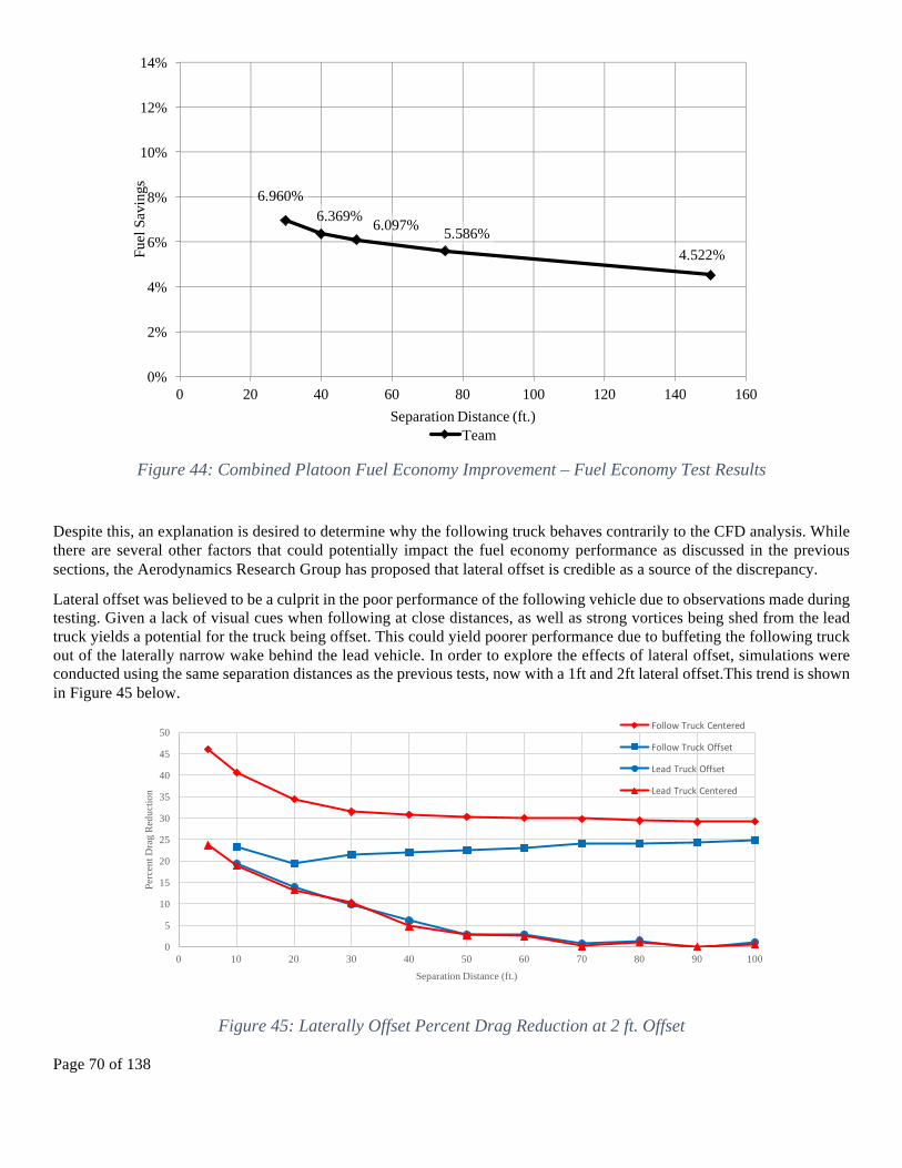
Page 70 of 138
Despite this, an explanation is desired to determine why the following truck behaves contrarily to the CFD analysis. While there are several other factors that could potentially impact the fuel economy performance as discussed in the previous sections, the Aerodynamics Research Group has proposed that lateral offset is credible as a source of the discrepancy.
Lateral offset was believed to be a culprit in the poor performance of the following vehicle due to observations made during testing. Given a lack of visual cues when following at close distances, as well as strong vortices being shed from the lead truck yields a potential for the truck being offset. This could yield poorer performance due to buffeting the following truck out of the laterally narrow wake behind the lead vehicle. In order to explore the effects of lateral offset, simulations were conducted using the same separation distances as the previous tests, now with a 1ft and 2ft lateral offset.This trend is shown in Figure 45 below.
Figure 44: Combined Platoon Fuel Economy Improvement – Fuel Economy Test Results
Figure 45: Laterally Offset Percent Drag Reduction at 2 ft. Offset
6.960%6.369% 6.097% 5.586%
4.522%
0%
2%
4%
6%
8%
10%
12%
14%
0 20 40 60 80 100 120 140 160
Fuel
Sav
ings
Separation Distance (ft.)Team
0
5
10
15
20
25
30
35
40
45
50
0 10 20 30 40 50 60 70 80 90 100
Perc
ent D
rag
Redu
ctio
n
Separation Distance (ft.)
"#$$#%!&'()*!+,-.,',/
"#$$#%!&'()*!0112,.
3,4/!&'()*!0112,.
3,4/!&'()*!+,-.,',/

Page 71 of 138
The percent drag reduction trend, which can be directly linked to the fuel performance trend, is demonstrably closer to that realized by test results from both NREL’s testing 4 and the fuel economy tests from TRC. While not quite the same level of degradation at the close spacings, the wake expands behind the truck in the lateral direction, and thus when the trucks are closely spaced, there is a larger portion of the truck removed from the beneficial slipstream. This makes the impact of the lateral offset more important at close spacings. Additionally, the vortices shed by the lead truck diminish in strength as they propagate, therefore the closer the vehicles to each other, the more likely they are to be buffeted off center. This compounds the issue of lateral offset, which potentially explains the reversal of the following truck’s trend at close following distances. The lead truck, however, receives nearly the exact same benefit even when not laterally offset. This is most likely due to the mechanism for the lead truck’s drag reduction still being highly effective even when partially offset. While being offset, the following truck still manages to break up the low pressure region behind the lead truck, yielding performance gains.
Shown above in the two feet lateral offset case, which represents an operating maximum for the vehicles. Despite this, the platoon sees degradation in the performance at even small lateral offsets. Shown below is the percentage drag increase for an offset of only 8 inches, a much more realistic average offset during operation.
From Figure 46 it can be concluded that lateral offset degrades the drag reduction performance, with close spacings having a much larger degradation then the further spacings. This leads credence to its relevance in the discussion about potential culprits for the unexpected fuel economy trend.
It is still worth nothing however, that the combined platoon still receives optimal benefit at the closest spacings, due to the large gains the lead truck experiences. Therefore, for two-truck platooning, the ideal spacing for the trucks was determined to be as close as is safe for implementation of the system.
Figure 46: Following Truck 8 inch Lateral Offset Percent Loss from Zero Offset Platooning
0.00%
0.50%
1.00%
1.50%
2.00%
2.50%
3.00%
3.50%
4.00%
4.50%
0 10 20 30 40 50 60
Perc
ent L
oss
Separation Distance (ft.)

Page 72 of 138
E. Conclusion In two-truck platooning, the lead truck overrides the unexpected downturn in following truck fuel savings at close following distances. Since the lead truck receives a 2% benefit near 50 feet, and a larger benefit at closer distances, it more than makes up for the loss of the following truck. It can be concluded then that for optimal two-truck platoon fuel economy performance, the platoon trucks should be spaced as close as is safely feasible. Lateral offset is a potential culprit for the lesser performance of the following truck in close following distances and thus improving lateral control could potentially be an effective means for increasing the performance of the platoon. Further research and testing is needed to confirm this hypothesis.
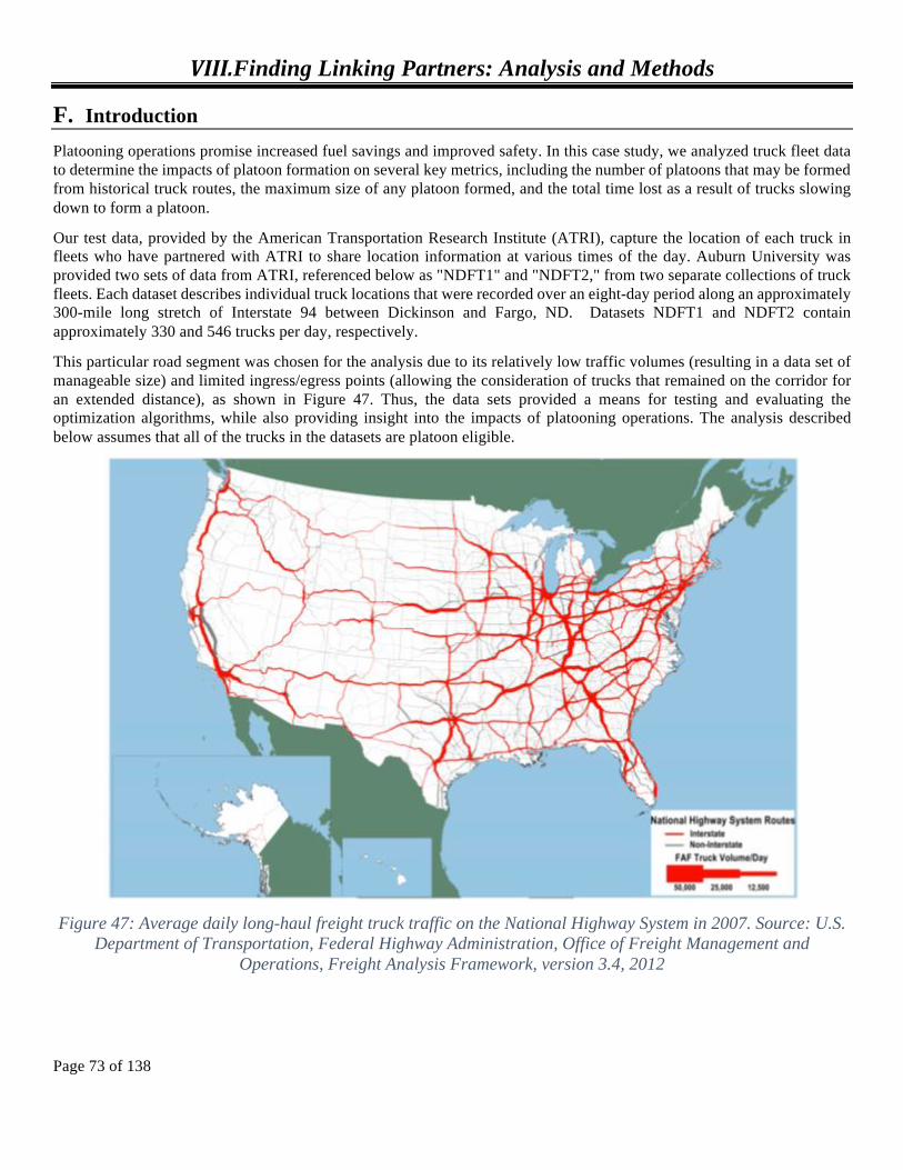
Page 73 of 138
VIII.Finding Linking Partners: Analysis and Methods
F. Introduction Platooning operations promise increased fuel savings and improved safety. In this case study, we analyzed truck fleet data to determine the impacts of platoon formation on several key metrics, including the number of platoons that may be formed from historical truck routes, the maximum size of any platoon formed, and the total time lost as a result of trucks slowing down to form a platoon.
Our test data, provided by the American Transportation Research Institute (ATRI), capture the location of each truck in fleets who have partnered with ATRI to share location information at various times of the day. Auburn University was provided two sets of data from ATRI, referenced below as "NDFT1" and "NDFT2," from two separate collections of truck fleets. Each dataset describes individual truck locations that were recorded over an eight-day period along an approximately 300-mile long stretch of Interstate 94 between Dickinson and Fargo, ND. Datasets NDFT1 and NDFT2 contain approximately 330 and 546 trucks per day, respectively.
This particular road segment was chosen for the analysis due to its relatively low traffic volumes (resulting in a data set of manageable size) and limited ingress/egress points (allowing the consideration of trucks that remained on the corridor for an extended distance), as shown in Figure 47. Thus, the data sets provided a means for testing and evaluating the optimization algorithms, while also providing insight into the impacts of platooning operations. The analysis described below assumes that all of the trucks in the datasets are platoon eligible.
Figure 47: Average daily long-haul freight truck traffic on the National Highway System in 2007. Source: U.S.
Department of Transportation, Federal Highway Administration, Office of Freight Management and Operations, Freight Analysis Framework, version 3.4, 2012

Page 74 of 138
We developed new optimization algorithms that determine which trucks should join to form a platoon, given the starting location of each truck. In particular, our analysis provides preliminary insights into the following metrics:
• Percent of trucks that join a platoon, • Number of platoons formed, • Number of trucks that were time delayed due to platooning operations, • Number of platoon formation operations (number of times vehicles adjusted speed to join a platoon), • Maximum platoon size at any given time, • Total time lost for trucks that platoon, • Distance traveled within platoon by individual trucks, • Percent of total distance traveled within a platoon, and • Total (estimated) fuel savings resulting from platooning.
The newly developed optimization algorithm is initialized with the location of each truck from the test data. The algorithm requires four key parameters. To form a platoon, a candidate lead truck may decelerate to fall back to join a trailing truck. In our analysis, we considered lead truck adjustment speeds of 5 and 10 miles per hour slower than the current speed. Similarly, the trailing truck may accelerate to join upstream trucks, with a trail truck adjustment speed of either zero or five miles per hour faster than the current speed. To limit the number of vehicles in a given platoon, the maximum platoon size parameter was set to two, three, or an unlimited number of trucks. Finally, the expected net fuel savings associated with forming and operating the platoon dictated the decision to couple trucks into platoons. We employed a Percent reduction in fuel cost for a platoon of either 5% or 10%, consistent with the published works of Larson et al. (2013) and Liang (2014)11,12. To improve the tractability of the models in the Phase 1 preliminary analysis, all vehicles in a platoon were assumed to realize the same fuel economy benefits. However, the Phase 2 analysis explicitly considered the differences in fuel economy benefits based on position within the platoon (e.g., the lead truck receives approximately half the fuel savings of a trailing truck).
Letting d1 be the distance from the trailing truck to the location where it meets the lead truck, dp be the distance traveled in platoon, v1 and v2 be the respective trailing truck and lead truck velocities, vp be the velocity of the trucks while in platoon, s be the percent reduction in fuel cost for a platoon, and Δv1 be the trail truck adjustment speed parameter value, we may determine whether trucks can feasibly platoon. For Equation (1), F1 is the fuel cost and ΔF1 is the fuel increased cost, meaning the extra fuel energy incurred from accelerating. Note that ΔF1 would be zero if the truck remains at a constant
speed. The fuel cost, F1, is measured by ( )21 10.5d v 11. Thus, Equation (1) is simply the fuel cost of traveling at the faster
speed (v1 + Δv1) minus the fuel cost of traveling at the normal speed (v1). Extending the idea of fuel cost to Equation (2), we obtain the equation for S, the fuel benefit from platooning. The first term of Equation (2) describes the fuel cost of truck 1 traveling at its normal speed for the distance that the trucks would have been in platoon if speeds were adjusted accordingly for platooning. Similarly, the second term describes the fuel cost of truck 2 traveling at its normal speed for the distance that the trucks would have been in platoon if speeds were adjusted accordingly for platooning. The third term describes the fuel cost of both trucks traveling at a common speed in platoon over the distance that they would platoon with a discount s. Thus, the discounted fuel cost from traveling in platoon is subtracted from the individual truck costs to get the fuel benefit from platooning.
ΔF1 = .5d1((v1 + Δv1)2 – v12) (1)
S = .5v12dp + .5v2
2dp - (2 - s).5vp2dp (2)
If the benefit from platooning is larger than the fuel increased cost, then the platoon should be formed and we may obtain the savings percent earned by calculating one minus the quotient of the expense incurred in the event of platooning over the expense incurred without any platooning or speed adjustments.

Page 75 of 138
1. Review of Phase One Findings
The preliminary analysis conducted in Phase One revealed several interesting observations. First, the percentage of fuel savings is only sensitive to the percentage of fuel reduction parameter and road saturation. This is the most surprising result, as the median savings is approximately 4%-7% regardless of the maximum allowable platoon size and adjustment speeds. It appears that the advantages and disadvantages of the parameters are normalized in the savings output. Second, the lead truck adjustment speed has a significant influence on the number of platoons formed. In particular, an increase in the lead truck adjustment speed (deceleration) results in the formation of additional platoons. However, a large lead truck adjustment speed also corresponds to increased time delays for platooned trucks.
One surprising result is that a trail truck adjustment speed of zero results in a greater number of platoons formed than when the trail truck speeds up by five miles per hour. The reason for this is that the cost of speeding up is a steep enough penalty to restrict platooning opportunities. However, a trail truck adjustment speed of five miles per hour enables longer distances traveled within a platoon by catching up to the platoon faster. A larger trail truck adjustment speed also decreases the time delay associated with platooning.
As the maximum platoon size increases, the number of platoons formed tends to decrease. This tendency is intuitive since large platoons absorb the platooning opportunity that could otherwise be distributed among several platoons of size two or three. Also, the percent of trucks that join a platoon tends to increase as the maximum platoon size increases. This is also intuitive since larger permissible sizes create more platooning opportunities.
Finally, the road saturation has a profound impact on the level of platooning opportunity. compares NDFT1 and NDFT2 by showing how many pairwise truck distances were within five miles, projected at 12:00 pm. on each side of the road. In particular, NDFT2 boasts more trucks with small pairwise distances than NDFT1, which is one reason that the results show more impressive platooning behavior for NDFT2.
One of the core project research questions addresses the relative likelihood that trucks will be able to find platooning partners, given typical distributions of trucks on highways. These findings show that, with this real-world dataset (which does not include all trucks on this highway section), formation of two-truck platoons among platoon-eligible trucks was 3-7% for NDFT1 and 30-45% for NDFT2. The differences depend on the parameters employed by the platoon formation model (e.g., allowable adjustment speeds for leading or trailing trucks). We find that trucks forming two-truck platoons in the NDFT1 dataset traveled within a platoon between 30-60% of the distance of the 300-mile road segment, on average. Trucks joining two-truck platoons in the more densely populated NDFT2 remained within a platoon between 55-75% of the road segment, on average (see Figure 48).

Page 76 of 138
New Findings from Phase 2
While the preliminary Phase 1 analysis revealed some useful general insights, several improvements to the analysis were identified for Phase 2. The particular improvements are described below.
First, a maximum allowable delay of 10-minutes was imposed in Phase 2 to prevent any truck from being excessively delayed as a consequence of joining a platoon. Thus, even if positive fuel savings would result from a truck joining a platoon, this operation was prohibited if it violated the 10-minute delay constraint.
One of the shortcomings of the Phase One analysis is that it ignored the impacts of a truck’s braking ability on the practicality of platoon formation. Thus, Phase Two considered the following three operational scenarios.
Scenario 1: Trucks may never change relative positions, and a trailing truck is not permitted to have worse braking ability than a leader truck in its platoon.
Scenario 2: Trucks may never change relative positions and a trailing truck is permitted to have any braking ability compared to its leader. However, the relative braking ability between the trucks determines the distance maintained between the vehicles when in platoon. The braking-dependent vehicle spacings, motivated by the work of Alam et al. (2014), are as follows13:
• A trail truck with worse braking ability than its leader travels 13 meters behind. • A trail truck with equal braking ability to its leader travels 2 meters behind. • A trail truck with better braking ability to its leader travels 0.5 meters behind.
Figure 48: NDFT2 has much higher road saturation than NDFT1

Page 77 of 138
While the exact gaps used in this analysis differ from the empirical work being conducted on the project’s test vehicles (and in some cases represent extremely aggressive spacing), the aim of this analysis was to capture the impacts of potentially widely-varying gaps on platoon formation strategies (and the corresponding fuel savings).
Scenario 3: Merging and weaving is permitted, which means that the relative truck positions may change over time, as new trucks are added to a platoon. In this scenario, trucks are always ordered from worst-to-best braking ability within each platoon (lead truck to trail truck).
To support this analysis, the braking ability of a given truck was categorized as being good, fair, or poor. Because such information was not available in the provided data sets, probabilities of each braking ability were assumed. A sensitivity analysis to determine the impacts of the assumed probabilities on platoon formation was conducted. The results indicate, surprisingly, that the results are not highly sensitive to the probabilities. Differences in the results due to changes in the probabilities are slight and seem to have no pattern. Three braking ability probability configurations were used in the sensitivity analysis for each of the three scenarios, making for nine total program runs. The three braking ability probability configurations are shown in Table 2.
Table 2: Braking ability probabilities for each configuration.
Braking Ability Good Fair Poor
Configuration 1 0.33 0.33 0.33 Configuration 2 0.05 0.90 0.05 Configuration 3 0.70 0.29 0.01
While Phase 1 considered unlimited platoon sizes, a more realistic maximum size of three was imposed in Phase 2. Furthermore, the lead truck adjust speed in Phase 2 was set to 10 mph, with a trail truck adjust speed of 5 mph (accelerating). Limiting the possible adjustment speeds enabled the team to focus the analysis on the impacts of the three operational scenarios.
Finally, the Phase 2 analysis explicitly considers fuel savings as a function of each truck’s position within the platoon. Thus, a truck’s savings is determined by the air drag ratio (drag reduction) it maintains while in platoon. The air drag ratio values depending on position and inter-vehicle distance are shown in Table 3 13,12. A small air drag ratio indicates large air drag reduction. By contrast, the Phase 1 analysis assumed that each vehicle within a platoon received the same fuel savings benefit.
Table 3: Air Drag Ratios depend on the distance between a truck and the truck directly in front of it (or behind it if it is the lead truck) and its position.
Distance between Trucks 13 Meters 2 Meters 0.5 Meters Lead Truck .98 .9 .85 One Truck Behind Leader .61 .55 .4 Two Trucks Behind Leader .55 .45 .35
It should be noted that the Phase 2 analysis utilized the same datasets employed in Phase 1 (namely, sets NDFT1 and NDFT2). Recall that both sets captured approximately 300 miles of I-94 between Dickenson and Fargo, ND. Between the two datasets, approximately 876 trucks per day were observed over an eight-day period.
The Phase 2 analysis employed the following two assumptions. First, velocity changes are assumed to be instantaneous. Velocity changes occur when a truck begins the coordination phase to merge into a platoon and when the coordination is complete and the trucks resume “normal” velocity. If a truck is not adjusting its velocity due to platooning operations, then

Page 78 of 138
its velocity is assumed to be constant. Next, we assume that a truck, when not platooning, consumes .1275 gallons of fuel per mile12.
2. Sensitivity Analysis
This section shows results that indicate how sensitive the variable braking ability probabilities for good/fair/poor categories are. Nine runs were performed using the three scenarios described above (s1, s2, s3) and the three probability configurations described above (pc1, pc2, pc3). Note that only a single day’s worth of data was chosen for these results (June 2, 2013) instead of the entire eight days of data (June 1 – June 8, 2013).
The general results of the sensitivity analysis indicate that the metrics of interest are not highly sensitive to the changes in brake category probabilities.
Figure 49 shows the total gallons saved across all trucks. While the total gallons saved may seem insignificant, this represents a savings of roughly 6-7% (as will be highlighted in subsequent figures). However, the purpose of this particular analysis was not to quantify actual fuel savings, but rather to assess the impacts of the braking ability scenarios. Thus, for scenarios 1 and 2, the total gallons saved does not seem to be impacted significantly by the probability configuration. For scenario 3, the total gallons saved is higher than the rest for configuration 1 and lower than the rest for configuration 2. The results are not highly sensitive to changes in the braking ability probabilities, except for scenario 3, in which case probability configuration 1 provides the most savings.
Figure 49: Fuel Savings vs. Scenarios

Page 79 of 138
It may seem odd initially that probability configuration 2 is the lowest for scenario 3, given that scenario 3 is the most flexible of all scenarios. However, probability configuration 2 assigns virtually all trucks the same brake ability; hence, most operations in scenario 1 and scenario 2 would accumulate very good savings despite the inability to change relative positions. In other words, scenario 3 no longer poses an advantage to the other scenarios when nearly all the trucks have uniform brake ability. Furthermore, scenario 3 heuristically assigns trail trucks to lead positions in the platoon, thereby causing trucks to accelerate and be placed in a less favorable position for earning savings.
Figure 50 shows the number of platoons formed. For each scenario, the probability configuration does not seem to make a large impact. The largest difference is about 10 platoons, which is given by probability configuration 1 and probability configuration 2 in scenario 2.
Figure 50: Number of Platoons Formed vs. Scenario

Page 80 of 138
Figure 51 shows how many operations were rejected due to the braking ability constraint of scenario 1. Recall that, in scenario 1, a platoon operation will be rejected if a truck catching up has worse brakes than the truck that will be its leader in the platoon. It seems that there is a significant difference in the results when comparing the probability configurations for scenario 1. Configuration 1 rejects about 100 more operations than configuration 2.
Figure 51: Number of Operations Rejected vs. Scenario

Page 81 of 138
Figure 52 shows the percent trucks that joined a platoon out of all the platoon-eligible trucks. Trucks are platoon-eligible if they are on the highway of interest and traveling at highway speed (e.g. not taking a rest break). For each scenario, it appears that the probabilities do not have a large impact on the number of trucks that join/merge. The largest difference occurs for probability configuration 1 and probability configuration 2 in scenario1, which is about 3%.
Figure 52: Percent of Trucks Joining Platoon vs. Scenario

Page 82 of 138
Figure 53 shows the percent distance traveled in platoon compared to the distance traveled on the road for individual trucks. All scenarios and all probability configurations seem to pose the same result for this metric. Hence, it does not appear that these results are sensitive to the probabilities
Figure 53: Percent Distance Traveled in Platoon

Page 83 of 138
Figure 54 shows the time delay incurred for individual trucks due to platooning operations. The median delays range from 4 to 16 seconds. It appears that these results are not sensitive to the brake probabilities. Recall that a maximum delay of 10 minutes was imposed. Negative delays are observed when trucks accelerate to form platoons with trucks that are further ahead on the roadway.
Figure 54: Time Lost due to Platooning

Page 84 of 138
Figure 55 shows the distance traveled in platoon by individual trucks. The median values are nearly the same for all combinations, ranging from 72.1 to 80.4, depending on the scenario and probability configuration. It seems that the results are not sensitive to the brake probabilities.
Figure 55: Distance Traveled by Individual Trucks

Page 85 of 138
Figure 56 shows the time delay per mile traveled for individual trucks. The results seem to not be sensitive to the brake probabilities, as the median values for all combinations tend to be around zero, with a median range from 0.15 to 0.59 seconds. Recall that a new constraint was added in Phase 2 to limit the total delay for any truck to be no more than 10 minutes. Thus, the larger delay rates are due to trucks slowing down to coordinate a platoon operation only to platoon for a relatively short distance.
Figure 56: Time Delay Traveled Per Mile Traveled

Page 86 of 138
Figure 57 shows the percent savings earned by individual trucks that join platoons. The results seem to not be sensitive to the brake probabilities (i.e., when isolating a particular scenario and comparing across probability configurations). Median values tend to be around 6% to 7%. Although it is counter-intuitive that scenario 1 boasts similar savings percentages to the other scenarios, the bar graphs in and do indicate that scenario 2 and scenario 3 tend to encourage more trucks to form platoons, which helps to validate the total gallon savings results. Thus, while scenario 1 leads to fewer platooning trucks, the fuel savings for those trucks that platoon is virtually identical to the savings exhibited under scenario 2.
Figure 57: Savings Earned (Percent)

Page 87 of 138
Figure 58 shows the fuel savings earned by individual trucks that merge into a platoon. These results do not seem to be sensitive to the brake probabilities. The median gallon savings tends to be around 0.75 gallons for each truck that joins a platoon. Since the results show no significant impact on savings for individual trucks that merge into a platoon due to varying scenarios or probability configurations, the importance of the number of trucks that join platoons to the total gallon savings is highlighted. In other words, varying scenarios and probability configurations are significant to the number of trucks that join a platoon (c.f., and ), and not significant to the savings that an individual truck earns, given that the truck has joined a platoon. Furthermore, it has been shown in that scenario 3 enables more trucks to join platoons than the other scenarios.
G. Phase Two Analysis Summary Results
The following figures show performance metrics and how they compare among the three scenarios. The results capture data recorded across all eight days available in the datasets. In this analysis, the probability of a truck having good brakes is assumed to be 0.5, the probability of a truck having fair brakes is assumed to be 0.3, and the probability of a truck having
Figure 58: Savings Earned (Gallons)

Page 88 of 138
poor brakes is assumed to be 0.2. These probabilities are roughly the averages from configurations 1 and 3, as described in Table 2.
The key result is that the total gallon savings is highest for scenario 3, then scenario 2, and it is lowest for scenario 1. In particular, the fuel savings in scenario 3 is roughly 6% higher than scenario 2 and approximately 13% higher than scenario 1.
Figure 59 suggests that enabling vehicles to perform merging into any platoon position (scenario 3) is beneficial. The fact that scenario 2 produces a 10.2% higher savings than scenario 1 indicates that, if merging/weaving is not possible, then at least permitting trucks to platoon at potentially high inter-vehicle distances is beneficial. Scenario 3 boasts a 6.3% reduction in fuel savings over scenario 2 and a 17.2% reduction versus scenario 1. For scenario 1, the average number of operations rejected due to the braking ability constraint was about 33 operations (averaged per day across all trucks). This may be a key reason why scenario 2 out-performed scenario 1.
Figure 59: Total Gallons Saved
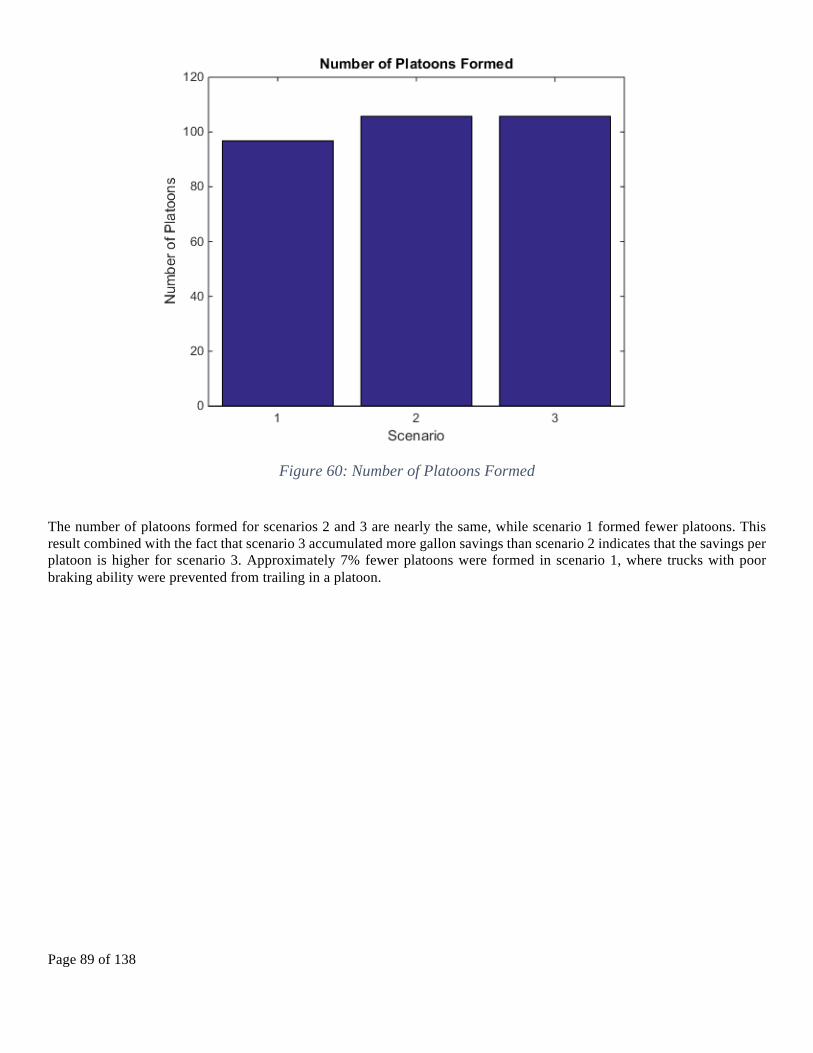
Page 89 of 138
The number of platoons formed for scenarios 2 and 3 are nearly the same, while scenario 1 formed fewer platoons. This result combined with the fact that scenario 3 accumulated more gallon savings than scenario 2 indicates that the savings per platoon is higher for scenario 3. Approximately 7% fewer platoons were formed in scenario 1, where trucks with poor braking ability were prevented from trailing in a platoon.
Figure 60: Number of Platoons Formed

Page 90 of 138
The percent of trucks that joined a platoon is actually highest for scenario 2, not scenario 3 (with scenario 2 besting scenario 3 by roughly 3% and scenario 1 by nearly 12%). Recall that the objective of the optimization algorithm is to maximize the total savings. It has been shown above that scenario 3 generates the largest total gallon savings. Hence, since scenario 3 is the most flexible, it assigned trucks to platoons more efficiently.
Figure 61: Percentage of Trucks that Joined a Platoon

Page 91 of 138
The percent trucks that lost time is highest for scenario 2. This result corresponds with the result that the most trucks joined platoons for scenario 2.
Figure 62: Percent of Trucks that Lost Time

Page 92 of 138
The time lost for individual trucks is virtually the same across all scenarios. The median tends around zero. Some trucks are delayed up to the maximum allowable delay of ten minutes, while some trucks actually gained about eight or nine minutes of time mostly due to trail trucks accelerating during the coordination phase of the platoon operation.
Figure 63: Time Lost Due to Platooning

Page 93 of 138
The distance traveled in platoon by individual trucks is virtually the same across all scenarios. The median distance traveled in platoon is about 75 miles.
Figure 64: Distance Traveled in Platoon
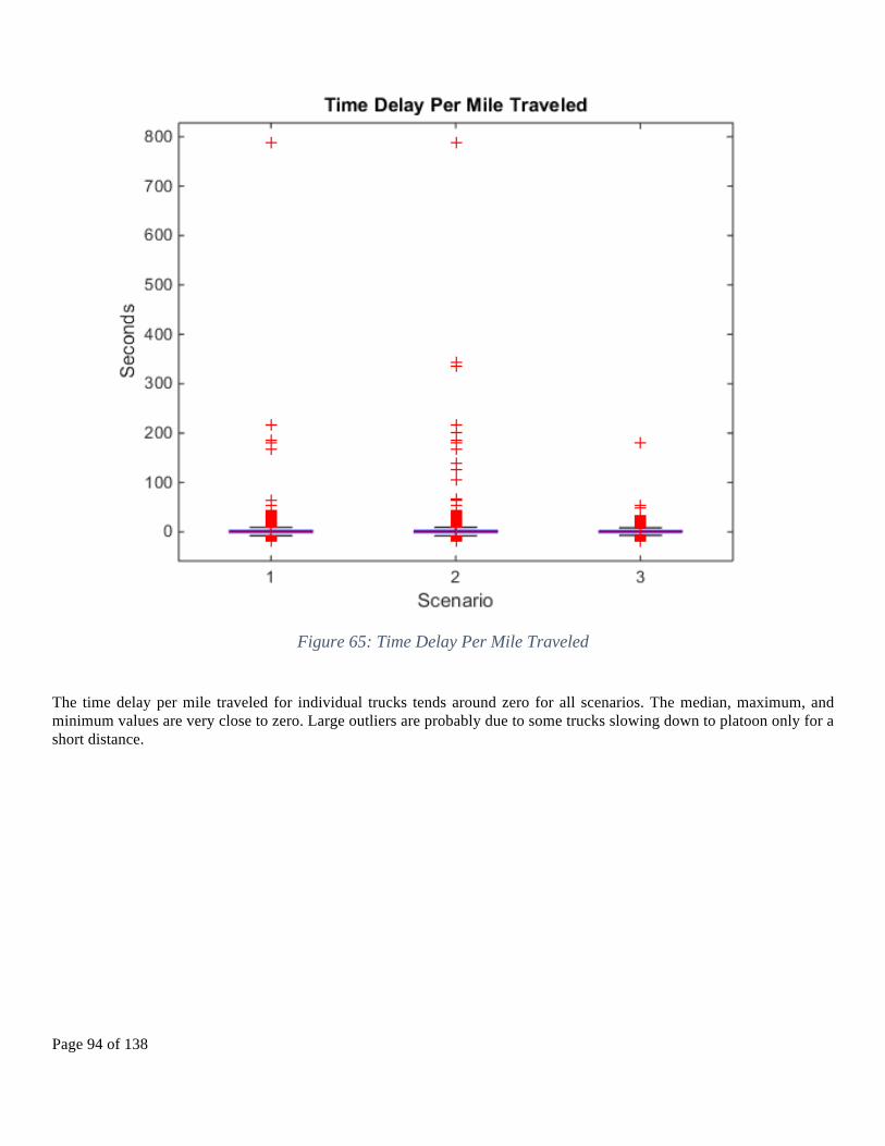
Page 94 of 138
The time delay per mile traveled for individual trucks tends around zero for all scenarios. The median, maximum, and minimum values are very close to zero. Large outliers are probably due to some trucks slowing down to platoon only for a short distance.
Figure 65: Time Delay Per Mile Traveled

Page 95 of 138
This figure describes the distance that individual trucks travel in platoon compared to the distance that the individual trucks travel on the road. These results are virtually the same across all scenarios. The median value tends around 70%.
Figure 66: Percent of Total Distance Traveled While Platooning
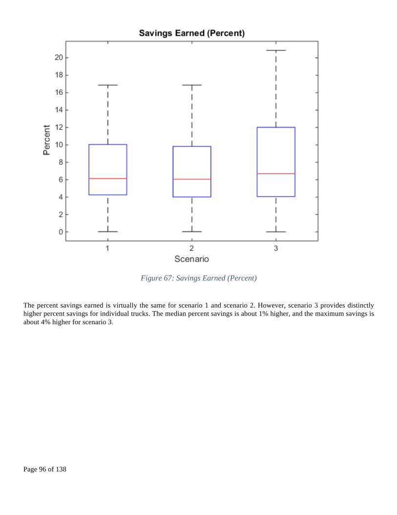
Page 96 of 138
The percent savings earned is virtually the same for scenario 1 and scenario 2. However, scenario 3 provides distinctly higher percent savings for individual trucks. The median percent savings is about 1% higher, and the maximum savings is about 4% higher for scenario 3.
Figure 67: Savings Earned (Percent)

Page 97 of 138
The gallon savings earned for scenario 3 (median of 0.73) is slightly better than the savings for scenario 1 (median of 0.68) and scenario 2 (median of 0.64). It appears that there are more outliers gaining high gallon savings for scenario 3.
Figure 68: Savings Earned (Gallons)

Page 98 of 138
IX.IX.
IX.Potential Traffic Flow and Mobility Impacts
A. Methodology This section of the report describes the traffic analysis tasks undertaken in the second phase of the project. In the first phase, traffic simulation modeling was used to estimate the impacts of DATP on traffic flow during peak hour conditions on a 5.3-mile segment of freeway in a small urban area. In this second phase, the traffic modeling effort was expanded to address a wider range of scenarios. Phase two work includes: modeling the peak hour of truck traffic on the 5.3-mile segment of freeway used in phase one, modeling one of the interchanges on that segment in isolation from the rest of that segment, and modeling an extended rural freeway segment without interchanges. As with the first phase work, for each of the three models described above, a baseline case representing existing conditions was developed, followed by a series of model cases in which market penetration of trucks with DATP capability was varied among 20, 40, 60, 80, and 100% across a series of headways of 1.25, 1.0, 0.75, and 0.5 seconds for the advanced technology vehicles. Finally, models for the range of parameters described above were executed at the current traffic volume and increases of 15% and 30%, to represent potential growth in traffic volume over the long term.
The traffic microscopic simulation software used for the further study of freeway sections is CORSIM. The TSIS Next version of CORSIM is used, since it has a capability to model advanced technology vehicles in the traffic stream, which TSIS 6.3 version cannot accomplish. TSIS Next consists of a text editor, and the model geometry, time periods and other parameters can all be altered to carry out trial runs. CORSIM has a stochastic nature, which is helpful in replicating the non-uniform nature of real traffic conditions. For our study, we have created three new vehicle types in CORSIM: advanced technology single unit truck, semi-trailer with medium load and double bottom trailer. Percentage of different types of trucks used in this study is varied for each model run depending on the market penetration of advanced technology vehicles into the traffic stream. For headway distribution of non-advanced technology vehicles, the default sensitivity factors are used, which are different for 10 driver types, reflecting the nature of drivers in the real traffic. On the other hand, the distribution of time headways for advanced technology vehicles are kept constant for the 10 driver types, but are varied among different cases to see the difference in traffic flow with different headway values. A Pitt-car following constant of 10 feet/second is used. This value is a constant, and is added to the results of a car following sensitivity calculation to determine the car following separation distance. The Pitt-car following constant however, is used only for non-advanced technology vehicles. All the other parameters, such as vehicle acceleration or deceleration characteristics, are maintained at default values set by the software.
The site selected for the first simulation model study is a 5.3-mile segment of a roadway from south of Exit 58 to north of Exit 62 on Interstate 85 in Alabama. This segment has 3 interchanges within the study area. This study considered the simulation of the peak hour of truck traffic in the traffic stream. As the data pertaining to the truck classification in each hour is not provided in the ALDOT traffic data website, this model used the percentage distribution of different types of vehicles in the traffic stream from a weigh-in-motion station’s data for the month of March, 2015. This station is located 25 miles to the south of the study segment. The vehicle type distribution was assumed to not have much difference from the actual traffic in the study section because the area between the study segment and the weigh station consists of farmlands, and does not have a particular destination for trucks. The peak hour truck traffic was calculated, and those percentages were applied to the total number of vehicles in the traffic stream in that hour between Exits 58 and 62.
The second simulation model was that of an isolated interchange. The isolated interchange used for this simulation was Exit 60 of the previous study segment, devoid of any basic freeway segment. The aim of this simulation was to study the effects of platooning, when the truck platoon enters an interchange until it exits it. Exit 60 has partial cloverleaf interchange geometry. The data used for this model is the same as the previous model with the entire freeway segment. From the weigh-in-motion data obtained from the station, the peak hour of truck traffic was found to be the 18th hour of the day. The traffic volume obtained from the ALDOT website is given as AADT. The AADT is converted to hourly count by multiplying it by the K factor (proportion of daily traffic occurring during the peak hour and D factor to give the peak hour volume and traffic volume in the dominant direction, respectively. The K factor used for the first and second models was 0.1 and the
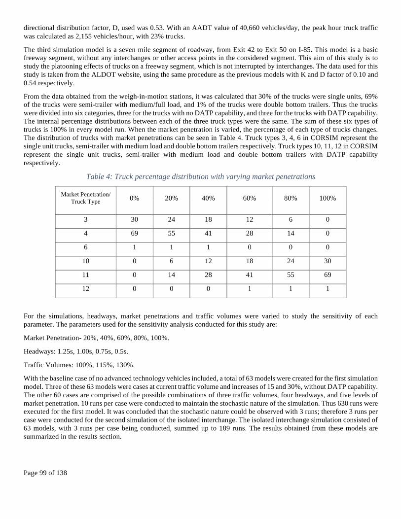
Page 99 of 138
directional distribution factor, D, used was 0.53. With an AADT value of 40,660 vehicles/day, the peak hour truck traffic was calculated as 2,155 vehicles/hour, with 23% trucks.
The third simulation model is a seven mile segment of roadway, from Exit 42 to Exit 50 on I-85. This model is a basic freeway segment, without any interchanges or other access points in the considered segment. This aim of this study is to study the platooning effects of trucks on a freeway segment, which is not interrupted by interchanges. The data used for this study is taken from the ALDOT website, using the same procedure as the previous models with K and D factor of 0.10 and 0.54 respectively.
From the data obtained from the weigh-in-motion stations, it was calculated that 30% of the trucks were single units, 69% of the trucks were semi-trailer with medium/full load, and 1% of the trucks were double bottom trailers. Thus the trucks were divided into six categories, three for the trucks with no DATP capability, and three for the trucks with DATP capability. The internal percentage distributions between each of the three truck types were the same. The sum of these six types of trucks is 100% in every model run. When the market penetration is varied, the percentage of each type of trucks changes. The distribution of trucks with market penetrations can be seen in Table 4. Truck types 3, 4, 6 in CORSIM represent the single unit trucks, semi-trailer with medium load and double bottom trailers respectively. Truck types 10, 11, 12 in CORSIM represent the single unit trucks, semi-trailer with medium load and double bottom trailers with DATP capability respectively.
Table 4: Truck percentage distribution with varying market penetrations
Market Penetration/ Truck Type 0% 20% 40% 60% 80% 100%
3 30 24 18 12 6 0
4 69 55 41 28 14 0
6 1 1 1 0 0 0
10 0 6 12 18 24 30
11 0 14 28 41 55 69
12 0 0 0 1 1 1
For the simulations, headways, market penetrations and traffic volumes were varied to study the sensitivity of each parameter. The parameters used for the sensitivity analysis conducted for this study are:
Market Penetration- 20%, 40%, 60%, 80%, 100%.
Headways: 1.25s, 1.00s, 0.75s, 0.5s.
Traffic Volumes: 100%, 115%, 130%.
With the baseline case of no advanced technology vehicles included, a total of 63 models were created for the first simulation model. Three of these 63 models were cases at current traffic volume and increases of 15 and 30%, without DATP capability. The other 60 cases are comprised of the possible combinations of three traffic volumes, four headways, and five levels of market penetration. 10 runs per case were conducted to maintain the stochastic nature of the simulation. Thus 630 runs were executed for the first model. It was concluded that the stochastic nature could be observed with 3 runs; therefore 3 runs per case were conducted for the second simulation of the isolated interchange. The isolated interchange simulation consisted of 63 models, with 3 runs per case being conducted, summed up to 189 runs. The results obtained from these models are summarized in the results section.

Page 100 of 138
B. Results All the simulations were carried out by changing one factor and keeping others constant, to check the sensitivity of the results to each factor in the model. The numeric results for the first model network, consisting of the entire freeway section between Exit 58 and Exit 62, are shown in Table 5, Table 6, and Table 7. Those three tables show the variation of market penetrations with varying headways for 100%, 115% and 130% of the current traffic volumes respectively. The speeds of the baseline cases are also accounted for in the table. The trends that can be seen in these results are shown in the graphs following the tables.
Table 5: Average Speed Results for Entire Freeway Section at Current Volume
Baseline:68.77 MarketPenetration
Headway 20% 40% 60% 80% 100%
1.25s 68.92 69.03 69.10 69.14 69.20
1s 68.95 69.01 69.11 69.19 69.26
0.75s 68.99 69.03 69.13 69.17 69.24
0.5s 68.95 69.03 69.17 69.21 69.26
Table 6: Average Speed Results for Entire Freeway Section at 115%
Baseline:68.35 MarketPenetration
Headway 20% 40% 60% 80% 100%
1.25s 68.43 68.40 68.53 68.55 68.72
1s 68.44 68.35 68.53 68.57 68.76
0.75s 68.42 68.52 68.66 68.79 68.88
0.5s 68.55 68.55 68.64 68.73 68.92
Table 7: Average Speed Results for Entire Freeway Section at 130%
Baseline:67.16 MarketPenetration
Headway 20% 40% 60% 80% 100%
1.25s 66.89 67.11 67.34 67.37 67.69
1s 67.19 67.23 67.33 67.76 67.96
0.75s 67.19 67.32 67.62 67.78 67.92
0.5s 67.23 67.38 67.54 67.93 68.01
Charts plotting the variation of market penetration and speeds at different headways are shown in Figure 69, Figure 70, and Figure 71. A common trend that can be seen is that, within each market penetration value, as the headways decrease from 1.25 seconds to 0.5 seconds, the speeds increase. This implies that as the vehicles move at a shorter headway, there is a

Page 101 of 138
tendency for speed to increase. This trend is seen at all three different traffic volumes, although it may not be consistently increase in each combination of market penetration and traffic volume.
Figure 69: Average speeds of vehicles at different market penetrations and different headways at 100% traffic volume
Figure 70: Average speeds of vehicles at different market penetrations and different headways at 115% traffic volume
68.50
68.75
69.00
69.25
69.50
20% 40% 60% 80% 100%
Spee
d (m
ph)
Market Penetration
1.25
1.00
0.75
0.50
68.00
68.25
68.50
68.75
69.00
20% 40% 60% 80% 100%
Spee
d (m
ph)
Market Penetration
1.25
1.00
0.75
0.50

Page 102 of 138
While looking at a particular headway for different market penetrations, it can be seen that all the different combinations of headways and traffic volumes showed an increase in mean speed. As an example, the graph showing variation of speeds at different market penetrations for 0.75 seconds headway at 115% of the current traffic volumes is shown in Figure 72.
On viewing the variation of headway over a particular market penetration and traffic volume (in this example, 20% market penetration and 115% traffic volume) in the Figure 73, it can be seen that there is hardly any variation in the speeds, and all
Figure 71:Average speeds of vehicles at different market penetrations and different headways at 130% traffic
volume
Figure 72: Distributions of Speeds at different market penetration for a headway of 0.75 seconds at 115%
traffic volume
66.00
66.25
66.50
66.75
67.00
67.25
67.50
67.75
68.00
68.25
20% 40% 60% 80% 100%
Spee
d (m
ph)
Market Penetration
1.25
1.00
0.75
0.50
68.00
68.25
68.50
68.75
69.00
20% 40% 60% 80% 100%
Spee
d (m
ph)
Market Penetration
0.75s Headway at 115% traffic volume

Page 103 of 138
the variation is within a range of 0.25 mph. This is true for all the cases. Thus it can be said that for any particular market penetration and traffic volume, a change in time headway does not cause a substantial change in the speeds of vehicles.
However, an interesting observation that could be seen in Figure 69, Figure 70, and Figure 71 is that, although the trends are increasing for each headway and market penetration, the overall speeds pertaining to increasing traffic volumes are decreasing. As an example, Figure 74 shows a plot of average speed for 60% market penetration and 1 second headway. Astraffic volumes increase, average speed showed a declining trend. The same is true for all the cases. Thus we can say that at any given market penetration and headway, the speeds show a declining trend in regards to increases in traffic volume.
The second model which was considered was that in which an interchange was isolated from the larger segment. This model was developed to see the changes in traffic parameters like speed and delay associated with platoons in an interchange alone.
Figure 73: Average speeds at different headway distribution for 20% market penetration for 115% traffic volume
Figure 74: Average speeds of vehicles at different traffic volumes for 60% market penetration and 1 second
headway
68.00
68.25
68.50
68.75
69.00
69.25
69.50
1.25s 1s 0.75s 0.5s
Spee
d (m
ph)
Headway
20% Market Penetration
88:AA
8;:AA
89:AA
8F:AA
!""#$ !!%#$ !&"#$
!"##$%&'
"()
*+#,#-.%.+/0012%3456'#

Page 104 of 138
The same parameters were applied and the results were noted, as can be seen in Table 8, Table 9, and Table 10. The baseline cases are also noted for comparison in the tables.
Table 8: Average Speed Results for Isolated Interchange Section at 100%
Baseline:69.24 MarketPenetration
Headway 20% 40% 60% 80% 100%
1.25s 69.19 69.22 69.17 69.15 69.22
1s 69.26 69.15 69.20 69.14 69.23
0.75s 69.26 69.07 69.22 69.34 69.15
0.5s 69.25 69.21 69.30 69.26 69.26
Table 9: Average Speed Results for Isolated Interchange Section at 115%
Baseline:68.34 MarketPenetration
Headway 20% 40% 60% 80% 100%
1.25s 68.39 68.48 68.92 68.20 68.62
1s 68.81 68.75 68.78 68.61 68.25
0.75s 68.40 68.50 68.70 68.72 68.80
0.5s 68.31 68.81 68.53 68.82 68.97
Table 10: Average Speed Results for Isolated Interchange Section at 130%
Baseline:66.94 MarketPenetration
Headway 20% 40% 60% 80% 100%
1.25s 66.19 66.83 67.18 66.27 67.60
1s 67.37 66.75 67.63 67.25 67.34
0.75s 66.40 67.13 66.84 67.72 67.42
0.5s 65.44 66.37 66.34 66.62 66.91
Figure 75, Figure 76, and Figure 77 show the speed variations for time headway and market penetration distributions for 100%, 115%, and 130% of the current traffic volumes, respectively. It can be seen from the graphs that the distribution does not show a particular trend. The speeds for 100% of the current traffic volume hardly show any variations, with all the speeds above 69 mph. It can be seen that 115% traffic volume graph may be showing a few trends, but they are within each time headway. The 130% traffic volume graph shows random variations which do not exhibit any trend. It is suspected that the very short segment being modeled was not long enough for trends to emerge and overcome any random noise in the models.

Page 105 of 138
The third model considered in this phase of the study was that of an extended basic freeway segment in a rural area. This model was simulated to observe the changes in traffic parameters like speed and delay associated with platoons in a freeway segment devoid of any interchanges. The parameters that were altered to study the sensitivity analysis were the same as the previous two models, and the values are noted in Table 11,Table 12, and Table 13 for 100%, 115% and 130% of the traffic volumes, respectively. The baseline case results are noted in the top right corner of every table.
Figure 75: Average speeds at different headway distribution and market penetration for 100% traffic volume
Figure 76: Average speeds at different headway distribution and market penetration for 115% traffic volume
Figure 77: Average speeds at different headway distribution and market penetration for 130% traffic volume
65.00
66.00
67.00
68.00
69.00
70.00
1.25 1 0.75 0.5
Spee
d (m
ph)
Headway (seconds)
20%
40%
60%
80%
100%
65.00
66.00
67.00
68.00
69.00
70.00
1.25 1 0.75 0.5
Spee
d (m
ph)
Headway (seconds)
20%
40%
60%
80%
100%
65.00
66.00
67.00
68.00
69.00
70.00
1.25 1 0.75 0.5
Spee
d (m
ph)
Headway (seconds)
20%
40%
60%
80%
100%
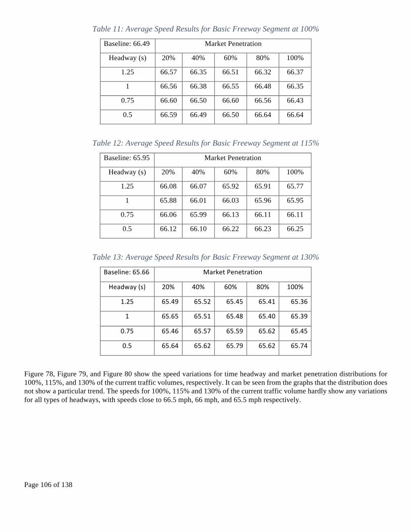
Page 106 of 138
Table 11: Average Speed Results for Basic Freeway Segment at 100%
Baseline: 66.49 Market Penetration
Headway (s) 20% 40% 60% 80% 100%
1.25 66.57 66.35 66.51 66.32 66.37
1 66.56 66.38 66.55 66.48 66.35
0.75 66.60 66.50 66.60 66.56 66.43
0.5 66.59 66.49 66.50 66.64 66.64
Table 12: Average Speed Results for Basic Freeway Segment at 115%
Baseline: 65.95 Market Penetration
Headway (s) 20% 40% 60% 80% 100%
1.25 66.08 66.07 65.92 65.91 65.77
1 65.88 66.01 66.03 65.96 65.95
0.75 66.06 65.99 66.13 66.11 66.11
0.5 66.12 66.10 66.22 66.23 66.25
Table 13: Average Speed Results for Basic Freeway Segment at 130%
Baseline:65.66 MarketPenetration
Headway(s) 20% 40% 60% 80% 100%
1.25 65.49 65.52 65.45 65.41 65.36
1 65.65 65.51 65.48 65.40 65.39
0.75 65.46 65.57 65.59 65.62 65.45
0.5 65.64 65.62 65.79 65.62 65.74
Figure 78, Figure 79, and Figure 80 show the speed variations for time headway and market penetration distributions for 100%, 115%, and 130% of the current traffic volumes, respectively. It can be seen from the graphs that the distribution does not show a particular trend. The speeds for 100%, 115% and 130% of the current traffic volume hardly show any variations for all types of headways, with speeds close to 66.5 mph, 66 mph, and 65.5 mph respectively.

Page 107 of 138
Figure 78: Average speeds at different headway distribution and market penetration for 100% traffic volume
Figure 79: Average speeds at different headway distribution and market penetration for 115% traffic volume
Figure 80: Average speeds at different headway distribution and market penetration for 130% traffic volume
8C:AA
8E:AA
88:AA
8;:AA
89:AA
D:@E D A:;E A:E
'"#$
("#$
)"#$
*"#$
!""#$
8C:AA
8E:AA
88:AA
8;:AA
89:AA
D:@E D A:;E A:E
'"#$
("#$
)"#$
*"#$
!""#$
8C:AA
8E:AA
88:AA
8;:AA
89:AA
D:@E D A:;E A:E
'"#$
("#$
)"#$
*"#$
!""#$

Page 108 of 138
X.Conclusion and Recommendations
Within this project, technical and engineering evaluations have significantly extended understanding of key factors relevant to DATP. Wireless communications investigations deepened our understanding of DSRC performance in trucking environments. Detailed investigations of platoon formation strategies have produced and quantified several options for the industry to consider regarding finding DATP linking partners, while traffic modeling has shown DATP operation to create no disruptions to overall traffic flow. Fuel economy testing yielded data that suggests that the DATP system provides a significant net improvement in fuel savings, while some results indicate that further research is needed to understand the trend of fuel savings for the following truck at close distances.
Of primary importance to the aim of the overall project, business case analyses have shown that DATP operations are highly likely to be feasible for a substantial portion of trucking operations, and that key fleets clearly see this value. Concerns held about specifics of DATP operation are natural for a new technology; this project has defined key requirements that need to be fulfilled for fleets to have confidence to adopt these systems. In Phase One, we concluded that large, for-hire, over-the-road (OTR) truckload (TL) and less-than-truckload (LTL) line-haul fleets and private fleets are best positioned as early adopters of DATP, due to their financial resources and operational aspects including freight lane density and trip length. While other sectors and fleet sizes are potential target markets, the larger OTR fleets have the opportunity to resolve key challenges and lower adoption prices through economies of scale. These conclusions are consistent with the views of trucking industry executives interviewed in Phase Two, who provided insight into near-term commercial evaluation and deployment of DATP. Potential customers will prioritize safety assurance, examining issues of system interoperability, integration with collision mitigation systems, and cooperative braking dynamics. Through development and application of “real-world” operational scenarios for target platooning markets, further research and early deployment of DATP should aim to validate the roadway types, driving conditions, truck networks and actual commercial DATP systems that will enable early adopters to recognize a return on investment. Even in the near term, realistic scenarios are likely to evolve rapidly as DATP functionality expands, for example, to integrate with lower speed applications such as freight signal priority on arterial roads.
The fuel economy testing yielded data that suggests that the DATP system provides a significant net improvement in fuel savings. However, some characteristics of the fuel savings observed indicate that further investigations are needed to understand the trend of fuel savings for the following truck at close distances (in the 30 foot range). Lateral offset is a potential culprit for this trend, and thus improving lateral control could potentially be an effective means for increasing the performance of the platoon. Furthermore, the data set analyzed for fuel economy investigations was highly limited, given the many variables that will arise in real-world deployment, such as vehicle weight, speed, trailer type, and tractor type. Further research and testing is needed to confirm new hypotheses and broaden the data set.
In two truck platooning, the lead truck allows the fuel economy trend to continue to increase at closer spacings. Since the lead truck receives a 2% benefit near 50 feet, and a larger benefit at closer following distances, it more than makes up for the decline in following truck fuel savings at close distances. It can be concluded then that for optimal two truck platoon fuel economy performance, the platooning trucks should be spaced as close as is safely feasible.
While key research questions have been identified, it is important to return to the question of near term deployment, i.e. commercial feasibility. Based on team expertise plus engagement with the trucking industry, first generation DATP systems are expected to run with inter-vehicle spacings of 50-75 feet. Based on fuel economy improvements observed in testing, a strong business case exists for introducing this technology. In general, the extensive track testing helped support the overall hypothesis that DATP technology is near market ready.
Driver Assistive Truck Platooning offers the potential to lead to new levels of freight/fleet efficiency and improved mobility for all highway travelers, while substantially reducing trucking-based emissions from long-haul trucking and enhancing the V2X communications environment.
The research team offers the following recommendations for future research: ● Additional detailed track testing is needed to understand the aerodynamics or other control system impacts of DATP
at close following distances. Further investigation of offset would require measurement of the positions of both tractors and trailers within a platoon.
● It is important to explore the difference between trucks and trailers that have different aerodynamic profiles relative

Page 109 of 138
to the conditions they produce in their wake, in real-world platooning tests. Further dedicated testing could include land vehicle coastdown testing (SAE J1263 [10]) to correlate to CFD drag reduction numbers, heavy-duty vehicle cooling tests (SAE J1393 [11]) to further characterize engine compartment conditions, or further joint TMC/SAE J1321 Type 2 fuel consumption tests at various vehicle weights, configurations, and longitudinal or lateral offsets. In all cases, some modifications to the test procedures must be made to accommodate two-vehicle tests with a lead and following truck held at a constant following distance.
● It would be useful to evaluate technical and societal parameters of further applications likely to emerge from the deployment of DATP equipped trucks when not platooning, such as signal priority on arterials with heavy freight traffic.
● It is important that findings from this project be clearly and accurately presented to the trucking industry and government stakeholders going forward, given the current media environment in which even low automation systems such as DATP tend to be inaccurately labeled with terms such as “driverless.”
Page 110 of 138
XI.Appendix A
XII.
FuelConsumptionforaPlatoonofClass8TractorTrailers
Raymond Schubert, Josh Switkes, John Jacobs - Peloton Technology, Inc. Lowell Brown, Luke Humphreys - Auburn University
Richard Bishop - Bishop Consulting
Abstract
Experimental results of the fuel economy benefits of an automated tractor-trailer platooning system are reported and the trends are analyzed. Data was collected in accordance with the joint TMC/SAE J1321 Fuel Consumption Test Procedure – Type II (1986) at the Transportation Research Center in East Liberty, Ohio.
Introduction
In addition to increased safety, autonomous vehicles also allow for a greater management of fuel resources. This improvement in fuel economy is realized through several strategies from design of the overall system traffic flow down to low-level vehicle controls. In the middle of the spectrum is coordinated adaptive cruise control (CACC), which is also referred to as driver assistive truck platooning (DATP) or platooning, for short.
The platooning strategy takes advantage of multi-body aerodynamic relationships and makes use of the many of the sensors employed for an increasing level of autonomy. These sensors include position and velocity measurements from GPS, as well as range to adjacent vehicles information from radar and dedicated short-range communication (DSRC). Command coordinated vehicle accelerations must also be communicated between vehicles. The vehicle-to-vehicle (V2V) communication requirement is handled by a DSRC system. The sensors and system processing allow for significantly quicker intervention and corrective action in comparison with the response time of a human. Thus, much shorter following distances are safely facilitated by the CACC system compared to those safely used with manual driving.
Measureable fuel benefits of DATP have been revealed in prior research. However, DATP systems are still in developmental stages and recent studies provide fuel savings analysis for only a handful of velocities and following distances. Recent studies within the United States by [1] Browand, [2] Roeth, and [3] Lammert have found similar savings at comparable velocities and following distances. [1] Browand found average following truck fuel savings to be 10% and team fuel savings of 8% at ten meter spacing for tandem operated trucks traveling around 50-55 mph. In [2] Roeth, testing found the following truck savings averaged 10% and lead truck savings 4.5% at 64 mph, 12m following distance only and at about 4200 ft altitude.
A more recent study by [3] Lammert showed improvements to be 9% for the following truck and around a 6% team average for fuel savings at 65 mph and 65,000 lb. This study also explored speeds between 55-70 mph, weights between 65,000 lb and 80,000 lb and following distances of 20 -75 ft. Still, because of various ambient conditions and the state of the development platooning system, results may not reflect a best-case or upper threshold for fuel savings improvement.
Additional studies [4-7] have also been performed on the European cab-over truck design. The results from cab over design research indicate similar fuel improvements as seen in studies using standard truck cab configurations. Platoons containing more than two trucks have also been considered [6, 7] and the experimental data reveals fuel improvements depend on the relative location of the truck in the platoon.
The on-road fuel economy testing present here was a part of a project funded by the Federal Highway

Page 111 of 138
Administration (FHWA) titled Heavy Truck Cooperative Adaptive Cruise Control: Evaluation, Testing, and Stakeholder Engagement for Near Term Deployment. This project is led by Auburn University and includes a project team of Peloton Technology Inc. (Peloton), American Transportation Research Institute (ATRI), Peterbilt Trucks, and Meritor WABCO. Peloton led the Type II fuel economy test effort. Peloton and Auburn University researchers performed the tests with instrumentation and data collection support from the National Renewable Energy Laboratory (NREL).
The need for new fuel economy testing came from two main motivations. First, Peloton’s platooning system that was used for [2] Roeth, and [3] Lammert had undergone further development to address some issues that potentially impact fuel economy. The issues were likely due to strict following distance control and inability to control the powertrain in an integrated way. The trucks used in previous studies had manual transmissions instead of the Automated Manual Transmission (AMT) of these test trucks and what is anticipated as standard for CACC trucks in deployment. Second, the team at Auburn University had performed computational fluid dynamics (CFD) analysis of a two-truck platoon that required real world data for model verification. The experiments were carried out to provide fuel economy analysis for a two-vehicle platoon of semi trucks loaded to 65,000 lb over following distances ranging from 30 to 150 ft.
Background and Methods
Test Design
To build on the knowledge gained by previously completed tests of Peloton’s prototype platooning system, the speed, vehicle weighing and following distance configurations were chosen to overlap with existing data while expanding understanding of greater following distances. The 65 mph and 65,000 lb loading case provided the most data points from [3] Lammert’s study. While safety concerns from the test facility limited the closer following distances, the test was able to expand the testing of following distances to 150 ft.
To adhere to the joint TMC/SAE J1321 Type 2 procedure, at least 3 runs within a 2% measurement error were required at each data point. It was determined that the minimum of 3 runs would be completed during a single test session (within a day) so that the measurement error could be calculated before moving forward to the next following distance test configuration. The order of following distance tests was randomized prior to the start in an attempt to minimize further environmental impacts.
Multiple baseline test sessions were conducted in an attempt to capture the changing environment over the several weeks of testing.
Test Track
The 7.5-mile oval test track at the Transportation Research Center (TRC) in East Liberty, Ohio has four asphalt lanes and banked turns. The turns have a radius of 2,400 ft and parabolic bank that increases in bank angle as a vehicle moves from inner to outer lanes. The fuel economy tests were run in lane one which has an effective bank angle of 10 deg. in the turns. The straight sections run parallel to the NW axis and are two miles in length. The straights are largely flat, however there is a 0.25 % slope down towards the NW direction of the track. Figure 81 represents a satellite image of the TRC facility with North towards the top of the page.
Figure 81: Transportation Research Center Test Facility, largest oval is the 7.5-mile test track (Image http://citr.osu.edu/resources.html)
Vehicle Specifications
Peterbilt Trucks supplied newer model 579 tractors with aerodynamics packages in support of the FHWA project led by Auburn University. Tractors with the aerodynamics package are fast becoming the standard across the transportation industry. The trucks used in this study are compliant with the SmartWay guidelines specified by the Environmental Protection Agency (EPA). As mentioned in [1] it is likely the preliminary rulemaking of the EPA Phase 2 greenhouse gas emissions and fuel efficiency standards will make aerodynamic

Page 112 of 138
improvements standard for new Class 8 trucks. SmartWay compliant trailers were rented and loaded for a combined test weight of 65,000 lb. Refer to Table 17 for exact load values and distributions for each truck. Table 1contains the specifications of the tractors and trailers used for the lead, follow and control vehicle respectively.
Table 14: Specifications for Test Tractors and Trailers
Specification Lead Tractor- Trailer
Follow Tractor-Trailer
Control Tractor-Trailer
Manufacturer Peterbilt Peterbilt Peterbilt
Model 579 579
579
Model Year 2014 2014 2013
Vehicle Mileage at Test End
6,595.9 mi 6,524.7 mi 16,173 mi
Engine Manufacturer
Paccar Cummins Cummins
Engine Model MX-13
ISX15 415 ST2
ISX15 415 ST2
Engine Model Year 2014
2014
2013
Emissions Equipment
DDI, TC, CAC, ECM, EGR-C, OC, SCR-U, PTOX
EGR, PTOX, SCR
EGR, PTOX, SCR
Transmission Eaton Fuller Automated 10-speed
Eaton Fuller Automated 10-speed
Eaton Fuller Automated 10-speed
Retarder/ Regenerative Braking
Engine Brake Engine Brake Engine Brake
Tires (Front Axle) Michelin X Green XZA3
Michelin X Green XZA3
Bridgestone Eco Pia R283
Tires (Driven Axles)
Michelin Energy XDA
Michelin Energy XDA
Bridgestone Eco Pia M710
Trailer Configuration
53 ft Van Trailer with angled side skirts
53 ft Van Trailer with angled side skirts
53 ft Van Trailer with angled side skirts
Trailer Manufacturer
Wabash Wabash Wabash
Trailer Model TRA VAN DVCVHPC
TRA VAN DVCVHPC
TRA VAN DVCVHPC
Trailer Height 13’ 6” 13’ 6” 13’ 6”
Trailer Width 102” 102” 102”
King Pin Set Back 36” 36” 36”
Trailer Axle Longitudinal Position
40’ 40’ 38’
Trailer Side Skirt DuraPlate AeroSkirt
DuraPlate AeroSkirt
DuraPlate AeroSkirt
Tires (Trailer Axles)
Goodyear Fuel Max Tech G316 LHT
Goodyear Fuel Max Tech G316 LHT
Goodyear Fuel Max Tech G316 LHT
Distance from Rear of Trailer Side Skirt to Front of Trailer Wheels
36” 36” 10-12”
A prototype platooning system developed by Peloton Technology Inc. (Peloton) was used during the test. The system is comprised of a radar sensor, GPS receivers, cameras, DSRC radio for vehicle-to-vehicle communication and a small-form CPU. The CPU is also interfaced with the J1939 CAN bus and provides vehicle braking and torque controls while platooning. Both the
lead and follow vehicles are equipped with the hardware described in detail in Table 2. The CPU of the follow vehicle is designated as the primary device and takes authority of the brake and throttle while in DATP mode. Currently, the system does not control lateral position, so the driver must remain responsible for keeping the truck in the lane. The driver also has ability to apply the brakes above and beyond command of the DATP system at any time.
Table 15: Peloton System Specifications Device System Description Radar (lead) Stock Meritor WABCO unit for ACC
Mounted in front bumper Radar (follow) Delphi Electronic Scanning Radar:
Dual beams Short range +/- 45 deg. beam, 60 m range Long range +/- 10 deg. beam, 175 m range 20 Hz update rate Mounted in front bumper
Dedicated Short Range Communications Denso DSRC Radio WSU 1.5 Dual antennas in diversity mode Omni-directional antennae mounted on side of sleeper cab Single 10 MHz channel Single-board computer and 5.9 GHz DSRC radio Supports IEEE 802.11p, P1609.3, P1609.4, P1609.2
Vehicle Communication Bus J1939 CAN interface via interface card in an embedded PC Private CAN network for sensors J1939 for vehicle bus and actuation
ABS/Stability Control (Lead) Meritor WABCO Brakes ESC
ABS/Stability Control (Follow) Bendix Brakes ESC
Figure 82: Lead Tractor and Trailer

Page 113 of 138
Figure 83: Follow Tractor and Trailer
Test Procedures
The joint TMC/SAE J1321 Fuel Consumption Test Procedure – Type II (1986) was referenced for the testing procedure [8]. During phase 1 of the FHWA project, ATRI inquired about the preferred method of testing and found that the Technology and Maintenance Council (TMC) of the American Trucking Associations (ATA) prefer the 1986 version of the SAE procedure. Furthermore, the mileage requirements in the 2012 SAE J1321 for all test trucks was impractical to meet within the project timeline on the trucks that were supplied by Peterbilt trucks. However, the joint TMC/SAE J1321 Type II standard was developed for assessing the fuel economy of a single vehicle. To characterize the fuel economy of a platooning system of multiple vehicles some modifications were made to the procedure and analysis.
The primary modification was that two test-to-control (T/C) ratios were required, because there were two vehicles under test. A T/C ratio for the lead vehicle and second T/C ratio for the follow vehicle were calculated. Additionally, a physical modification was made to the fuel delivery system of the platooning trucks: an electronically-switched solenoid valve was installed to the existing fuel lines to accommodate switching the supply between an auxiliary tank and the standard saddle tanks. This switch allowed the auxiliary tank to be activated precisely so that the only fuel drawn from the auxiliary tank was used during constant velocity platooning. Fuel needed to enter the track and accelerate into the platoon formation was pulled from the standard saddle tanks. The switch also included a status signal that was logged by the Peloton system, which published that signal to the J1939 CAN bus. This method ensures fuel consumed from the auxiliary tank could be attributed only to conditions during platooning.
The control truck had a removable auxiliary fuel tank similar to the ones used on the test trucks added. However, permission was not granted to install an electronically-switched solenoid valve on the fuel line. To accommodate the differences in fuel line set up, the control truck ran a full seven laps on test. Thus, the auxiliary tank for the control truck would be on test beginning with engine ignition in the pit area of the track and ending with engine halt upon return to the pit area. This means that the control truck burned more fuel than the test trucks, but that the difference was consistent between test runs. Since the two test vehicles were similar in setup, it was determined that a single control vehicle was acceptable for both test vehicles.
On the test track, at speed and at designated following distance, both the lead and follow trucks would simultaneously switch to the test tank on each respective truck when the platoon reached the 4.8-mile mark. Radio communication was used to coordinate the switch to the auxiliary test tanks. The lead and follow trucks had required observers on-board to aid the driver in communication and to monitor the platooning system. On the seventh lap, the fuel would be switched off the test tanks and back to the saddle tanks at the same 4.8-mile marker. Thus, the lead and follow trucks were considered on test during 6 platooning laps –for 45 miles. The T/C ratio calculation was not affected (provided the procedure was consistent between runs).
Other steps taken for consistency included settings for the climate control of the truck cab and exhaust restrictions. The air conditioning unit was turned off, the windows were closed and the fan speed was set to 75% of maximum. Previous testing revealed that the diesel particulate filter (DPF) system engages the exhaust regeneration process rather frequently especially if the engine experiences extended periods of idle run time. The DPF regeneration process injects fuel into the exhaust to aid in the removal of particulate build up and therefore invalidates a test run. To prevent this, the DPF regeneration was disengaged during data collection. Additionally, care was taken to limit idling of the engines and the switch was engaged during the 1-hour warm-up period to allow any necessary regeneration cycles to occur.
A full warm-up was performed prior to data collection often at the beginning of each day. The full warm-up procedure incorporated the following:
• All vehicles were driven for approximately an hour at a speed of 60 mph around the 7.5-mile track
• For the lead and follow trucks, the fuel was drawn from the saddle tanks

Page 114 of 138
• The control truck used a designated travel auxiliary tank during warm-ups
• All trucks were spaced at least 500 ft apart • DPF regeneration switches were engaged
After the warm up the trucks would stop at the pit area and prepare for a test run. The travel tank of the control truck would be switched to a new test tank. The lead and follow trucks would install a new test tanks. All test tanks had their starting weight measured and recorded. Idle between warm-up and test runs was limited to less than five minutes. The test run procedure was marked by:
• Three complete test runs at 65 mph for each following distance • For each test run, the lead and follow trucks left the pit area
within a few seconds of each other, with the exception of baseline runs
• Lead and follow trucks accelerated to cruising speed. Once follow truck was in range of the lead truck the platoon system was engaged.
• Three minutes after the lead and follow trucks departed the pit area the control truck would start test. The total run time of the control truck is recorded with a stopwatch.
• On lap one, at the 4.8-mile marker, the lead and follow trucks switched electronically to test tanks and began data collection
• On lap seven, again at the 4.8-mile marker, the lead and follow trucks electronically switched from the test tanks to the saddle tanks and end test data collection
• At the end of lap seven, lead and follow trucks pulled into pit area test tanks were removed. A second set of previously weighed full test tanks were then installed.
• Three minutes later, the control truck pulled into pit area and was off test after a minute idle. The end of test occurred at ignition halt and the test tank was replaced.
• While the control truck test tank was being removed the lead and follow trucks began another run
• After the test tank from the second test tank set was installed the control truck starts ignition and began another test run. The control truck remained three minutes behind lead and follow trucks.
• After all the trucks were on track the first set of test tanks were then weighed and data recorded
The primary measurement of concern was the ratio of the fuel used by the test vehicle, 𝑇, to the fuel used by the control vehicle, 𝐶. As discussed above this fuel economy test requires two T/C ratios. The fuel used by the lead vehicle is denoted 𝑇3 and the fuel used by the follow vehicle is denoted 𝑇*. The T/C ratio for lead and follow are then defined as
𝐿𝑒𝑎𝑑𝑇𝑟𝑢𝑐𝑘𝑇/𝐶𝑅𝑎𝑡𝑖𝑜 = BCD
(1)
𝐹𝑜𝑙𝑙𝑜𝑤𝑇𝑟𝑢𝑐𝑘𝑇/𝐶𝑅𝑎𝑡𝑖𝑜 = BHD
(2)
For a given test run within a set to be valid, it must lie within 2% of the runs in the set. The T/C ratio for runs
were checked as testing progressed. All fuel economy data presented in this paper falls within the 2% bound.
For fuel savings results, the T/C ratios for each vehicle at a designated following distance were compared to the T/C ratio of the baseline runs. Baseline runs were completed with at least 5000 ft following distance between test vehicles. The equations for the fuel savings are as follows:
𝐿𝑒𝑎𝑑𝑇𝑟𝑢𝑐𝑘𝐹𝑢𝑒𝑙𝑆𝑎𝑣𝑖𝑛𝑔𝑠 =MCN.OC
NOCN
(3)
𝐹𝑜𝑙𝑙𝑜𝑤𝑇𝑟𝑢𝑐𝑘𝐹𝑢𝑒𝑙𝑆𝑎𝑣𝑖𝑛𝑔𝑠 =MHN.OH
NOHN
(4)
Ambient Conditions Measurement
The ambient conditions were logged via an electronic weather station in the pit area of the track. The weather station measured the ambient temperature, relative humidity, average wind speed, peak wind speed, wind direction and barometric pressure. A range of conditions was observed during the three-week testing period. Usable test data was defined as having been collected when observed average wind speeds were within 3-10 mph, in accordance to the 1986 SAE Type II procedure. Average temperatures ranged between 62 degrees F and 81 degrees F. Finally, the relative humidity ranged from 39% to 82%.
Fuel Consumption Measurement
A gravimetric approach was used to measure the fuel consumption of the two test vehicles and the control vehicle. An auxiliary tank mount was fastened to the frame rails behind the cab and forward of the rear driven axles. The auxiliary tank was connected to the supply and return lines. As mentioned previously, the lead and follow trucks had an electronically-switched solenoid valve installed to facilitate switching between the saddle tank and auxiliary tank. The control truck did not have this capability, and a 3rd auxiliary “travel tank” was used for warm-up. Figure 4 shows the tank mount on the left and an auxiliary tank fastened to the mount is shown on the right.

Page 115 of 138
Figure 84: Left: Auxiliary tank mount Right: Auxiliary tank secured to mount and connected to fuel supply and return fuel lines
The mass of the test tanks on each truck was recorded prior to each run. Upon completion of a run the mass was again recorded. The difference in mass from the start and end of run represents the weight of fuel consumed during the test. Calibration of the scale was verified frequently with a known mass of 50 kg. Note, that the engine fuel rate as broadcast on J1939 was also recorded but serves only as a verification of the official consumed fuel weights.
Results
Gravimetric Fuel Economy Savings
Figure 85: Observed Fuel Savings versus Following Distance
The peak fuel savings for the following truck was found to be 10.24% at a following distance of 50 ft, and the peak fuel saving for the lead truck was 5.27% at 30 ft. The team fuel savings for was 6.1% at 50 ft. and 6.96% at 30 ft. Figure 5 represents the gravimetric fuel results where the percent fuel savings is plotted versus the respective following. Note that the percent fuel savings is used because it is a more conservative calculation for comparison than the percent fuel improvement and is likely the one more representative of savings during fleet operations. As the figure shows, there is a measureable benefit of the percent of fuel saved at all tested distances. Secondly, notice that as the distance between the two
trucks decreases the combined fuel savings steadily increases. The trend of savings for the following truck is non-monotonic. The fuel savings at a 30 ft following distance are less than the peak savings observed at 50 ft.This declining trend at the closest following distances also was observed during testing at Uvalde with NREL [3].
Last, it is noticeable that the follow truck fuel savings for long following distances does not sharply decrease. The CFD analysis suggests there is a decrease at some as of yet undetermined longer following distance. The fuel savings in Figure 5 indicates/confirms that this drop off occurs at a following distance beyond 150 ft. While the lead truck does not have a statistically significant fuel savings at 150 ft following distance (note the plotted confidence intervals at each point), the following truck -and therefore the team – numbers do appear to be significant.
As mentioned in the introduction, the need for this testing came from two main motivations. First, the Peloton Technology (Peloton) platooning system used in [2] Roeth and [3] Lammert had undergone further development to address some issues that potentially impact fuel economy.
Specifically, in these previous tests the strict gap or following distance control and the lack of integration with powertrain controls led to a harsh throttle control behavior while platooning at constant speeds (it should be noted that no brake commands were given during any of the FE testing at constant speeds). The harsh throttle control led to an increased rate of change in the torque demanded of the engine, which in turn lead to increased NOx emission rates and potentially contributed to the out-of-range engine temperature conditions that caused the engine fan of the following truck to engage at times. The rate of change in demanded torque increased as the following distance decreased – therefore leading to potential reductions in fuel economy savings at close following distances.
Since the time of the NREL test at the Uvalde test track [3], Peloton had made many evolutionary steps to integrate with the powertrain controls systems. Additionally, efforts to smooth out the torque demand were made to address potential NOx increases, as well as to potentially improve fuel economy. While increases in the (engine-out) NOx emissions rate often correspond to fuel economy gains, NREL proposed that the torque rate demands were high enough to produce off-cycle control issues for the engine that would negatively impact both NOx emissions and fuel economy. Additionally, the engagement of the mechanical engine fan during test runs would definitely impact fuel economy negatively.

Page 116 of 138
Observations from drivers and passengers before and during the test runs of the trucks at TRC noted a significant improvement in the control of the engine torque and that the engine fan did not engage at any time during the test. Most significantly, there was no observed change in the engine’s operating behavior at closer following distances when compared to further distances or baseline runs.
The second motivation for the testing was to provide the team at Auburn University with real world data for verification of their two-truck platooning CFD model. In order for the test track data to be used in this manner, we must understand if other factors are impacting results and are not easily modeled.

Page 117 of 138
Comparison to Previous Results
In the tests conducted in Uvalde, TX with NREL [3], a similar trend was identified for a platoon of trucks at 65 mph and 65,000 lb loading (see Figure 6). Those results showed a decline in following truck fuel savings at closer following distances from the values measured at 50 and 75 ft. The main attribute that was identified as a source of this unexpected trend was that the engine fan had turned on for a higher percentage of the test time at closer distances. This engagement of the engine fan leads to parasitic losses and decreases the fuel savings for these data points.
Figure 86: Observed Fuel Savings versus Following Distance from Uvalde, courtesy of NREL [3]
It was also observed that the engine commanded torque was oscillatory in nature and this could have contributed to unnecessary fuel consumption, higher NOx emissions, and possibly higher engine temperatures. Post processing of the platooning system data found that the following distance (gap) control effort was too restrictive – as the first generation DATP system developed by Peloton was designed to show the ability to strictly regulate the desired gap between paired trucks at close following distances.
Since those initial tests, refinements were made to the following distance control algorithm such that the control dynamics are characterized by a less aggressive calibrations and overall smoother control for driver comfort. Peloton’s prototype system also went from an electrically spoofed pedal position sensor signal to an integrated software solution using J1939 protocols through development efforts with engine manufacturers. The DATP system used in tests performed at TRC included these updates to the DATP controller.
Engine Temperature
During testing at TRC, four engine-temperature data channels were logged by the Isaac data loggers provided by NREL. Only two of those channels (engine intercooler temperature and engine oil temperature) were consistently logged for all three trucks. Figure 7 represents the engine coolant temperature versus time for the set of runs at 50 ft following distance while Figure 8 shows the engine oil temperature versus time for the same set of 50 ft following distance runs. These runs were chosen as examples because they show the general trend of temperature ranges that were measured during the test.
Figure 87: Engine Coolant Temperature at a following distance of 50 ft
The engine coolant temperature shows consistency within the individual trucks with no more than 2 degrees C variation during the runs except in the first lap of the control truck, where it appears to have cooled more rapidly between the test runs – even though it was idled and the engine cycled in a fashion similar to the test trucks.
The engine oil temperature displays a periodic signal that is correlated with the vehicle position on the track, likely due to the fact that there is a slight slope to the track in the northwest direction. Notice that the control truck’s engine has not completely warmed up for the first run of this 50 ft spacing set. This unexpected (and unobserved at the time of the testing) cool-down on the control truck occurred on several of the test runs. The rear truck engine is initially a little cool as well for the first run, but this was a less common occurrence.

Page 118 of 138
Figure 88: Engine Oil Temperature at a following distance of 50 ft
After the temperature level off from the initial warm-up, each of the three trucks appears to stabilize in a different temperature zone; the control truck ran hotter than the following truck, and the following truck ran hotter than the lead truck (at least as measured by the trucks’ own internal J1939 data channels). This could be because the follow truck was burning roughly 10% less fuel than the similar Cummins engine in the control truck and that the lead truck is a different engine (PACCAR). It also could have been due to the trucks actually having slight engine differences, or it could have been due to variance in the temperature sensors. It is important to note that all trucks were running well within normal operating temperatures and that the radiator fan never turned on during any of the test runs.
Figure 89: Mean Engine Coolant Temperatures versus Following Distance*
* Note that Following Distance on X-axis does not apply to control truck, which was at constant distance
Figure 9 shows the mean engine coolant temperatures for all three test trucks over the tested following distances. The error bars indicate the standard deviation of engine coolant temperature for the set of test runs at the respective following distance. While there are 5 tested following distances of 30, 40, 50, 75 and 150 ft, we also are including data from the baseline runs at roughly 5000 ft following distance between trucks and ACC runs of about 280 ft. A log scale is used on the X-axis to include all of these test distances (including the baseline runs) on one graph for identification of possible trends that correspond with the fuel savings result curves. Differences shown between baseline test runs and fuel economy test following distances would not statistical significance because of the manner in which this data was collected.
The lead truck for the prescribed following distance test runs retained a stock Adaptive Cruise Control (ACC) system from Meritor WABCO. As a potential baseline to some of the CACC operating conditions that were observed in previous Type 2 fuel economy testing, an attempt was made to capture data from the stock ACC system operating in the Type 2 environment. This would allow us to measure the engine temperatures, torque demand, longitudinal control and emission rates of the ACC for comparison to CACC performance. Upon inspection of the individual runs it was observed that the ACC system might have been disengaged for most of the duration of the first and last runs. Only the second run kept a consistent tracking of the lead vehicle. For these reasons the ACC run was omitted from the fuel economy v. following distance analysis.
The ACC runs did prove valuable for to comparing the ACC environment in several data looks and helps present a secondary baseline in many cases. In Figure 9, the temperature band is seen to follow the truck rather than the position in the platoon – as seen by the swapping of the lead and follow data points at the ACC distance of about 280 feet.
In previous tests at Uvalde [3], NREL had found that engine radiator fan turned on with a coolant temperature rise of between 7% and 8%. While the following truck showed some amount of increase in test runs over the baseline, the rise appears to be less than 1%

Page 119 of 138
Engine Torque
Figure 10 represents the filtered engine torque percent of the rear truck for several following distances. The quasi-periodic nature of the engine torque is due to a slight slope in the test track (as mentioned in the Test Track section). The control truck should cancel out variances in the fuel economy results due to environmental effects, including the slope in terrain. Test runs at a prescribed following distance were completed on different test days, so parameters measured by the J1939 of an individual truck could have an influence on the comparison by following distance. Recall that all runs presented here fell within the weather requirements, and the 2% repeatability factor as specified by the SAE Type II procedure.
Figure 90: Filtered Engine Percent Torque of the following truck
The average percentage engine torque shown in Figure 11 reveals that there is a local torque minima for the following truck for a following distance of approximately 50 ft. This corresponds to the peak of fuel savings for the following truck during the test.
Figure 91: Lead and Follow Truck Engine Torque Averages v. Following Distance
This minima in percent torque is interesting in that it reveals that the torque demanded to hold following distance begins to counter intuitively increase as the following distance approaches zero. This characteristic is contrary to the CFD simulations performed by Auburn for the project funded by the Federal Highway Administration (FHWA) titled Partial Automation for Truck Platooning Heavy Truck Cooperative Adaptive Cruise Control: Evaluation, Testing, and Stakeholder Engagement for Near Term Deployment. The CFD results are shown in Figure 12. The CFD analysis is further discussed in the SAE paper “An Evaluation of the Fuel Economy Benefits of a Driver Assistive Truck Platooning Prototype Using Simulation.” [9]
Figure 92: CFD Study Initial Results [9]
The CFD analysis found that aerodynamic efficiency continually improves as following distance decreases for both lead and following vehicles, which would suggest that the required engine torque should also decrease. Since the empirical test results do not match the CFD analysis, this hints at some unaccounted dynamics in either driver behavior, control behavior, engine conditions, or platoon aerodynamic interaction at close following distances. Note that the variation in engine torque averages across runs at each following distance is fairly tight (see Figure 11).
Engine Torque Rate Control & NOx Emission Rates
During testing of a protoype Peloton platooning system at Uvalde, NREL determined that the rate of change in engine torque commanded by the platooning controller increased as the following distance decreased. This was due to the fact that the control hardware and the control algorythm that was used during the test were developed primarily as a proof of concept of longitudual control on following distance, or “gap setting”. Since those tests in 2014, several developmental generations of the platooning software have addressed the concern of control smoothness and driver comfort. The mechanisms of the control also changed from a mechanical detent on throttle to an integrated software solution on commanded

Page 120 of 138
throttle, similar to production throttle control as used by cruise control or ACC systems.
Because of these changes, Peloton was confident they had addressed the variation in engine torque rate (also referred to as “ dither”) that was identifed as a potential issue for fuel savings, emissions, and excessive engine heat in the post-processing of the Uvalde data.
The calculation of emission rates relies on certain assumptions of the flow rate and environmental factors in order to convert from the J1939 measured PPM emission rate to a g/bhp-hr rate that is used for tailpipe emissions regulations. We will not try to recreate that analysis or provide a substitute. The average change in commanded torque can be found and plotted as a function of the following distance as a confirmation of the perceived improvement in control smoothness. This is done in Figure 13, which compares the mean change over a moving 0.2 sec window (which we will call “mean torque dither”) for the runs at TRC v. the Uvalde runs for the following truck. Also plotted are some following truck baseline runs and “induced dither” runs that were captured during Peloton’s development between the Type II fuel economy tests.
As Figure 13 shows, there remains a slight increase in mean torque dither for a following truck with an adaptive cruise control system (ACC or CACC) over the baseline cruise control runs due to a need to control to a transienttarget with some degree of elasticity. It is also seen that the TRC test runs don’t show a correlation of the rate change in torque increasing significantly as the following distance decreases, and there is particularly no difference in the control behavior at 30 ft and 40 ft when compared to 50 ft and 75 ft. Therefore we no longer believe the control of the throttle during platooning is having an impact on fuel savings, engine temperature increases or emissions.
Figure 93: Average change in torque of the following truck v. Following Distance
NREL supplied Isaac data loggers similar to those used at Uvalde to record the latest testing at TRC. Since the TRC testing, NREL separately analyzed the data for engine torque, average change in torque (or dither), and NOx emission rates. Their analyses are summarized in Figures 14 and 15.
NREL had hypothesized that while the engine speed remained constant, the engine torque command varied rapidly in the 2014 testing and that this resulted in a rapid variation in engine output was causing an increase in NOx. In order to quantify the rate of change in torque, the average change in percent torque measured over a 5 Hz window is reported in Figure 14. Note the thin black bars represent the standard deviation of the respective processed signal. This change in torque request, or mean torque dither, was 1.2 to 2.1 for the trailing vehicle in the 2014 tests, except for the baseline runs for which it was about 0.7. NOx in g/bhp-h was found to increase as the mean torque dither rate increased. In 2015, the mean torque dither rate was slowed to about 0.7 for the trailing vehicle and the NOx increase over baseline was largely eliminated (Figure 15).
Figure 94: Dither rate v. Following Distance for 2014 (Uvalde) and 2015 (TRC) trailing vehicles, courtesy of NREL

Page 121 of 138
The results from 2014 showed an increased in NOx emissions over the baseline in the following vehicle, despite the fact that less work was being done by the following vehicle. In Figure 15, the SCR Inlet data now shows total NOx decreases at all positions in reference to the NOx measured for the baseline runs.
Figure 95: Total NOx at SCR inlet v. Following Distance for 2014 (Uvalde) and 2015 (TRC) trailing vehicles, courtesy of NREL
Longitudinal Controller and Spacing Distance
While the previous experimental results with the Peloton DATP system showed a similar trend at close following distances (less than 50 feet), Peloton made great strides in refining the control and integration of the throttle to address control without compromising longitudinal control to the desired following distance. During the pre-test engineering phase of efforts at TRC the controller update was confirmed to be performing as designed on the test trucks.
To confirm the improvements had their desired impact, the data of following distance was first used to confirm that gap control was good. Figure 16 shows the average longitudinal distance, the following distance, between the test vehicles during the TRC fuel economy tests. For a clearer understanding of the controller performance the error in average following distance is represented in Figure 17. This shows that while the following distance control was refined and smoothed for comfort, this did not compromise the gap control significantly since the Uvalde tests [2].
Figure 96: Average Measured Longitudinal Offset v.Following Distance
Figure 97: Average Error of Measured Following Distance v. Following Distance
The longitudinal following distance for 30 ft following distance in Figure 17 reveals that at times there is slight variation in distance control. However, note that the relative position measurement from GPS receiver is measured/estimated via a raw position measurement andcould vary from roughly 1m down to 20 cm in accuracyat any given moment due to the cancelation of ionospheric and tropospheric errors that both receivers observe. But, over 12 to 24 hour period the average error for a differenced relative position be roughly 0.5 m. This has an impact on the drift in offsets versus time, which could be due to GPS or the trucks actual position. This effect should be reduced somewhat when the offset data for the full set of runs at each following distance are averaged. Specifically, the averaging of the offsets over the roughly 135 minutes of data for each set should bring the baseline GPS error closer to the .5 m expected measurement variance for a baseline calculated by positional differencing.

Page 122 of 138
Figures 18-19 show the longitudinal offset for a 30 ft. and 75 ft following distance respectively. The data has been filtered to only show GPS positions on the straights of the track, since lateral offset is difficult to calculate accurately on turns, even those with very large radiuses. Additionally, the data has been filtered against the quality of receiver position solutions. Specifically, the longitudinal and and lateral position solution standard deviations of the bestpos Novatel message were used as a quality threshold. The cutoff for the data was 1.95 m standard deviation. This value was chosen because it best eliminated positional drifts.
Both Figure 18 and 19 have the same time window that encompasses two laps with four straight sections. However only two of the four straight sections pass the quality threshold for the 75 ft run shown in Figure 19. These figures help show the frequency of the following distance or the following distance error, as measured by GPS over a period of two laps.
Figure 98: Longitudinal Offset for a single run at 30 ft Following Distance
Figure 99: Longitudinal Offset for a single run at 75 ft Following Distance
An examination of the velocity and tracking performance in Figures 20-21 of the speed versus time for 30 ft and 75 ft following distances suggests that the distance control is working well at maintaining a consistent following distance since the variance in velocity is roughly less than 0.1 mph. The mean and standard deviations of the speed for the lead and follow trucks for the set of runs are represented by Figure 22. Here, the low standard deviation observed visually in Figures 20-21 is confirmed in Figure 22.
Figure 100: Speed of Lead and Follow trucks at 30 ft Following Distance
Figure 101: Speed of Lead and Follow trucks at 75 ft Following Distance

Page 123 of 138
Figure 102: Mean Speed of Lead and Follow trucks versus Following Distance
Finally, Figures 23-24 are a sample of the visual tools used to confirm the straights have been removed. Figure 23 is an example from the 30 ft section and shows first that the straight sections were isolated. Figure 24 represents the positional data after the quality of receiver position solution threshold has been applied. A z-axis representing time was also added to the plot in Figure 24 to visually verify all of isolated sections for each lap of a given run. Observe that on what was defined as the back straight a large gap appears. This gap correlates with the location of an overpass.
Figure 103: Position of Lead and Follow trucks at 30 ft Following Distance
Figure 104: Time of Lead and Follow trucks at 30 ft Following Distance
Detailed Analysis of Results
The TRC test results show that the trend of fuel savings for the following truck is non-monotonic with a peak savings observed at 50 ft of 10.24%. This is also contrary to the CFD analysis, which found aerodynamic efficiency to continually improve as following distance decreases for both lead and following vehicles.
As the previous sections have shown, efforts were made to reduce or eliminate the conditions that were identified as likely contributors to this trend after the Uvalde tests [3]. Parasitic loads from the radiator fan and an unrefined control of torque showed improvement without compromising the ability of the platooning controller to maintain a consistent following distance. Therefore, more investigation was needed to characterize factors that could influence fuel consumption at closer distances.
Fuel Rate Confirmation of Fuel Economy
In an effort to verify the gravimetric Type II Fuel savings results, the team looked at the fuel rate available on J1939 for each of the test runs. This was not done to provide a potential substitute to the gravimetric results, but rather to ensure that no significant measurement errors occurred during the Type II procedure. The results of this investigation are plotted in Figure 25 for the lead truck and Figure 26 for the following truck.
Because there is usually small manufacturing variances in the fuel delivery system from truck to truck, the fuel rate as observed by the J1939 bus is not expected to match the fuel rate as measured by the Type II procedure. It is expected that any offset due to manufacturing variances would not change during the course of the test, so a consistent offset would be found regardless of following distance. Further, since the true measure of fuel savings is

Page 124 of 138
comparing a single truck while on test versus itself while on baseline – the fuel rate offset would cancel out in calculations made with the J1939 data.
This effort gave confidence that no significant measurement error occurred during the runs used for the Type II analysis. The joint TMC/SAE J1321 Fuel Consumption Test Procedure – Type II (1986)[8] also sets a repeatability metric of less than 2% run to run for each test, so it is likely that measurement or recording errors would have been caught at the time of testing.
Figure 105: Fuel rate for the set of runs v. following distance for the lead truck
Figure 106: Fuel rate for the set of runs v. following distance for the following truck
Detailed Engine Temperature Analysis
To further investigate engine temperature and environmental differences between the lead and following test trucks, comparisons were made to measurements of the control truck during the test runs. The control truck could help eliminate the influence of environmental factors on engine performance. Note that while temperature analysis and environmental analysis data
figures are plotted with Following Distance on the x-axis, the control truck data is presented for comparison but that the control truck following distance did not change during the course of the test. Therefore, in these cases the more accurate label for the X-axis may be “Test session for the Following Distance” instead of Following Distance. All test sessions for a following distance occurred on separate days.
For each set of following distances the engine oil temperature measurements were combined into a collections of data points for the entire set. The mean and standard deviation are then calculated from this collection of points for each respective set. Unless stated otherwise the averages and standard deviations for the figures presented are calculated from the collection of runs for a given set.
The engine oil temperature averages are shown in the Figure 27 plotted against the respective following distance for the test run. The vertical bars indicate the standard deviation of engine oil temperature for the set of test runs. The 280 ft following distance data correlates to the ACC test runs where a gap of 2.6 – 2.7 seconds was observed and that the test trucks were swapped in order during these runs so that the stock ACC system on the front truck could be used for test.
Figure 27 shows the trucks settling into separate zones that are offset from one another, again with the control truck highest, then the following truck, and lowest the lead truck. Note that temperature measured on the trucks during the ACC run (second longest following distance) fall within the band of the individual truck rather than their position in the platoon. In this one case, the truck with the Paccar MX-13 engine is the following truck.

Page 125 of 138
Figure 107: Mean Engine Oil Temperature v. Following Distance*
For the most part, the average temperature difference between the trucks remains the same. The differences in average temperature are also influenced by the conditions of the individual days in which the test runs were made. So when the lead truck and control truck show lower mean oil temperature for following distances of 30 and 40 feet, this is likely due to environmental factors on those days of test. The control truck should help filter out the day-to-day temperature, humidity and wind changes.
The lead and control truck show a similar pattern of mean oil temperature as they appear to show a decline in temperature at shorter distances. Yet, the following truck does not follow this trend. Figure 28 includes an exponential curve fit of the mean engine oil temperature for each spacing set. Observe that the temperature of the following truck seems to plateau at the closer distances while the lead and control temperatures drop. The ambient temperature was more than 10 degrees F lower on the 30 ft and 40 ft test days compared to temperature on the 50 ft and 75 ft test days. So the decrease in mean oil temperatures for the lead and control truck could be attributed to this environmental difference.
* Note that Following Distance on X-axis does not apply to control truck, which was at constant distance
Figure 108: Mean Engine Oil Temperature v. Following Distance with rational curve fit*
Referencing the front and rear trucks to the control truck should cancel out most of the environmental affects that could influence the engine temperature across the different testing days. Figure 29 represents the non-dimensional form of the engine oil temperature data for the lead and following trucks with the control truck used as the reference (note that the ACC distance data point is not included in the trend lines). It is observed that the temperature ratio of the following truck increases significantly more than the lead truck at the closer following distances. This ratio increase might be an indication that underhood temperature and flow conditions of the following truck are influenced by the following distance.
Figure 109: Mean Engine Oil Temperature divided by the control truck v. Following Distance*
It should be noted that it is believed that the engine oil temperatures observed throughout the Type II fuel economy testing were within the normal operating range
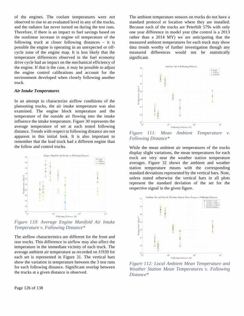
Page 126 of 138
of the engines. The coolant temperatures were not observed to rise to an evaluated level in any of the trucks, and the radiator fan never turned on during the test runs. Therefore, if there is an impact to fuel savings based on the nonlinear increase in engine oil temperature of the following truck at closer following distances – it is possible the engine is operating in an unexpected or off-cycle zone of the engine map. It is less likely that the temperature differences observed in the fuel economy drive cycle had an impact on the mechanical efficiency of the engine. If that is the case, it may be possible to adjust the engine control calibrations and account for the environment developed when closely following another truck.
Air Intake Temperatures
In an attempt to characterize airflow conditions of the platooning trucks, the air intake temperature was also examined. The engine block temperature and the temperature of the outside air flowing into the intake influence the intake temperature. Figure 30 represents the average temperature of set at each tested following distance. Trends with respect to following distance are not apparent in this initial look. It is also important to remember that the lead truck had a different engine than the follow and control trucks.
Figure 110: Average Engine Manifold Air Intake Temperature v. Following Distance*
The airflow characteristics are different for the front and rear trucks. This difference in airflow may also affect the temperature in the immediate vicinity of each truck. The average ambient air temperature as recorded on J1939 for each set is represented in Figure 31. The vertical bars show the variation in temperature between the 3 test runs for each following distance. Significant overlap between the trucks at a given distance is observed.
The ambient temperature sensors on trucks do not have a standard protocol or location where they are installed. Because each of the trucks are Peterbilt 579s with only one year difference in model year (the control is a 2013 rather than a 2014 MY) we are anticipating that the measured ambient temperatures for each truck may show data trends worthy of further investigation though any measured differences would not be statistically significant.
Figure 111: Mean Ambient Temperature v. Following Distance*
While the mean ambient air temperatures of the trucks display slight variations, the mean temperatures for each truck are very near the weather station temperature averages. Figure 32 shows the ambient and weather station temperature means with the corresponding standard deviations represented by the vertical bars. Note, unless stated otherwise the vertical bars in all plots represent the standard deviation of the set for the respective signal in the given figure.
Figure 112: Local Ambient Mean Temperature and Weather Station Mean Temperatures v. Following Distance*

Page 127 of 138
While overlap occurs in the ambient air data, a trend can be found through the use of the control truck. Figure 33 represents the ratio ambient temperature of the front truck to the control truck and the rear truck to the control truck respectively. This shows a trend towards higher local ambient temperature conditions for the following truck than the lead truck. This is likely due to the heat being generated by the lead vehicle – heat generated by engine, exhaust, and friction. In racing terms, this is known as running in “dirty air”. The trend shows that closer following distance produce a greater ambient temperature difference.
Figure 113: Local Ambient Mean Temperature of Lead and Following trucks divided by Control v. Following Distance*
Figure 34 represents the temperature difference of the rear from the front truck directly, with essentially no difference indicated for baseline runs. The front truck may be a better indication of control when investigating environmental factors because it should experience the closest conditions to that of the rear truck. This could be true for weather conditions as well as speed and traffic for tests not conducted on a closed test track at constant speeds. The less than 1 degree C temperature difference shown in Figure 34 is, again, not statistically significant and is likely within the margin of error of the ambient air temperature sensors. Still, the increasing trend at closer following distances is interesting and may be worthy of further investigation with higher accuracy sensors and tests designed to show a potential significant difference.
Figure 114: Difference of the Ambient Temperature of the Following from the Lead truck v. Following Distance
Higher ambient air temperatures around the following truck can influence the efficiency of the engine in a number of ways. This includes: the temperature of the air being ingested at the air filter; the efficiency of the turbo intercooler; the cooling of the engine block; and cooling of the intake manifold. To further investigate trends in some of these factors, the intake manifold and engine oil temperatures are shown in relation to the local ambient air temperature.
Figure 35 and 36 represent the ratios of engine manifold air intake temperatures to the local ambient air temperatures and the ratios of the engine oil temperatures to the local ambient air temperatures respectively. Based on the reference to the ambient air, it does appear that the intake temperature of the following truck has a lower manifold to ambient ratio than the Front and Control trucks. The ratio difference does appear to be present in the baseline and ACC runs, so it is likely due to sensor tolerance or the measurement error on the individual truck (remember that the follow truck becomes` the lead at only the ACC distance). This again points to the need for further testing with separate measurement sensors and test design to access potential differences due to following distances of platooning trucks. The engine oil to ambient ratio appears to be the similar in all three trucks.

Page 128 of 138
Figure 115: Ratio of Engine Intake Manifold to Ambient Air Temperatures v. Following Distance*
Figure 116: Ratio of Engine Oil to Ambient Air Temperatures v. Following Distance*
Environmental Factors
The presented weather data represents the aggregated weather station data. The data has been split up into sections that correlate with the time that individual test runs were executed. The data shown is also grouped together according to the following spacing distance of the test runs. Note that for most signals the weather station collects a windowed average of the logged signals. Non-averaged signals include maximum and minimum signals of the averaged window. For example, the “high temperature signal” is a record of the highest temperature observed during the averaging window for temperature.
The base line run includes five runs for the set. Three of those runs occurred on August 21 and the remaining runs occurred on August 19. Therefore, the baseline may display larger standard deviations in other weather station plots, these runs are represented with a following distance of 5000 ft The next furthest following distance is the ACC run and is at 280 ft.
Figure 37 shows the average and standard deviation of the windowed average temperature during each set of spacing distances. Note that all of the runs at a following distance occurred on separate individual days, with the exception of the baseline runs. It is interesting to note that the days in which the following truck experienced the highest fuel savings, at 50 ft and 75 ft following distance, occurred on the two warmest days. The unexpected downtrend of fuel savings at the closest following distances (30 ft and 40 ft) occurred on two of the coolest days.
Figure 117: Outside Air Temperatures v. Following Distance
Figure 38 represents the average wind speed. Observe that the average for each following distance is below the 12 mph ceiling for SAE fuel economy testing specifications. Also the standard deviation at each distance is well below 12 mph. The large standard deviation of the base line set is due to the set containing data from two different days.
Figure 118: Average Wind Speed v. Following Distance
Figure 39 shows the average peak wind speed during the ten-minute window. Note that average peak wind speed and the corresponding standard deviation suggest that

Page 129 of 138
data was collected below the peak wind speed ceiling of 15 mph.
Figure 119: Peak Wind Speed v. Following Distance
Figure 40 displays the average direction of the wind for the windowed average speed signal. The direction is represented in degrees heading where 0 deg. is North, 90 deg. is East, 180 deg. is South and 270 deg. is West.
Figure 120: Wind direction in the direction of Average Wind Speed v. Following Distance
The wind speed and direction data does not appear to have a strong correlation to the fuel economy results, particularly with respect to the unexpected downward trend at closer following distances. There does not appear to be a significant difference in the wind speeds of the runs at 50 ft and 75 ft compared to the 30 ft and 40 ft runs. The variation of wind direction does appear to be smaller on the days that 50 ft and 75 ft were run, but a platooning system would not seem to have a way to take advantage of this consistent environment. The test runs were completed with multiple laps around an oval track; so all directions of wind were experienced on all test runs.
Additional weather information plotted against the following distance is included in the next set of graphs,
Figures 41 – 44. Here again, no significant correlation to the fuel savings trend to following distance is indicated.
Figure 121: Average Pressure v. Following Distance
Figure 122: Dewpoint v. Following Distance
Figure 123: Heat Index v. Following Distance

Page 130 of 138
Figure 124: Humidity v. Following Distance

Page 131 of 138
Effects of Lateral Offset during Platoon
To better understand the apparent discrepancy between the percent fuel saved and the predicted aerodynamic drag, further CFD studies were undertaken as a part of the study. A more complete discussion of this work is available in the SAE paper “An Evaluation of the Fuel Economy Benefits of a Driver Assistive Truck Platooning Prototype Using Simulation” [9]. Of particular interest was the effect of relative lateral position between the lead and follow vehicles. Figure 45 depicts the percent drag reduction versus following distance for a relative lateral offset of two feet and of no offset. This offset distance was selected as a representative of a practical maximum offset during nominal DATP operation.
Figure 125: Percent Drag Reduction v. FollowingDistance with Lateral Offset
The drag reduction trend for the lateral offset case displays qualitatively similarities to track the measured trends in fuel saved during the TRC tests. Particularly notable is the changed inflection in the rear truck’s trend in conjunction with little observable change in the front truck’s profile. This suggests that the lead truck is affected by lateral offset far less than the following truck, possibly explaining why the rear truck’s inflection point is masked by the ideal case of perfectly centered platooning.
Considering the dynamics of the wake shedding off the front truck can suggest a possible explanation for this trend. With an offset, a portion of the rear truck is exposed to the undisturbed free-stream flow. This creates an asymmetrical pressure distribution on the front of that truck, as evidenced in Figure 46. This is likely due to vortex shedding off of the leading trailer working in tandem with the portion of the following truck exposed to the free-stream flow. As the separation distance decreases, the width of the wake also decreases, since the wake does not have time to dissipate in the longitudinal
direction. Thus, at close following distances, the effect of being offset seems to be exacerbated.
To help identify if lateral offset was a significant factor in the TRC testing, efforts were made to accurately quantify the relative position of the two platooning trucks to one another using available GPS data. Unfortunately, the Novatel rangeCMP message necessary for dynamic real time kinematic (DRTK) algorithm processing for an accurate relative position vector was not logged properly during the TRC testing. GPS data recorded with BESTPOS messages have estimated raw positional difference that could vary from roughly 1m down to 20 cm in accuracy at any given moment. But, over a 12 to 24 hour period the average error in baseline would vary byroughly 0.5m.
Figure 126: Pressure Contour on the Front Surface of the Following Truck with Outline of Lead Truck
To understand the potential impact of a lateral offset as indicated by the CFD modeling to the real-world track testing fuel savings, we must understand the magnitude, frequency, and duration of the lateral offset. While some amount of lateral offset will occur during testing, the percentage of time at an offset that is considered significant would seem to be a factor on the fuel savings.Figure 47 shows the time the test trucks were at an offset of 1 foot or greater and 2 feet or greater, as averaged across the test runs.
Note that the TRC 7.5-mile test track had marked lanes similar to those on the US highway system, with a 12-foot width. The tractor trailers are roughly 8 feet wide, so 2 feet exists on either side of a centered lead truck before the following truck would leave the lane or start crossing over the lane markings.

Page 132 of 138
Figure 127: Time at a 1 ft and 2 ft Lateral Position for Following Truck v. Following Distance
The percentage of time above 1ft and 2ft are represented in Table 3. The total time duration shown in the second column for each set includes only the acceptable GPS data. Recall that acceptable data is the GPS measurement data that meets the quality of position solution criteria discussed in the Longitudinal Controller and Spacing Distance section. Note, that a significant portion of data for the set at 150 ft following distance is excluded due to poor positional solution output from the GPS receiver. Nonetheless, the percent time above the lateral offset of 1 ft decreases as the following distance decreases, suggesting it may be easier for the driver to minimize offset at closer following distances.
Table 16: Percentage Time Above 1ft and 2ft Lateral Offsets
Percent Time Above Lateral Offset
Following Distance (ft)
Total Time (s) [of included data]
1 ft 2 ft
30 2661.5 0.00 % 0.00 %
40 3011.9 1.35 % 0.00 %
50 3781.0 1.12 % 0.00 %
75 2651.0 2.39 % 0.01 %
150 160.3 8.80 % 0.12 %
Another potential source of additional fuel consumption for the following truck may be from increased lateral oscillations by the following truck at close following distances. These lateral oscillations would cause small offsets that may be hard to measure with the available relative GPS data but could cause the following truck to be exposed to the free stream of air at narrow offsets. However, contrary to this hypothesis of increased lateral movements at closer following distances due to buffeting of air from the lead truck, Figure 48 shows that the oscillations become less pronounced as the following
distance decreases. Oscillations at any following distance can be explained by either driver behavior at these distances or by aerodynamic effects that are difficult to model in CFD or see in wind-tunnel analysis. Note that measured GPS differences are between the tractors and do not account for potentially larger oscillations that could occur between the trailers and the tractors, therefore the follow tractor may be further offset from the rear of the lead trailer than can be measured by this data set.
Figure 128: Lateral Positioning of Following Truck v. Following Distance
The decrease observed in Figure 48 in standard deviation of the lateral offset as the following distance decreases may indicate that the driver ability to hold on offset is not affected by buffeting. Observe that the mean of the lateral offset is nonzero for all distances and from 75 ft and below the mean lateral offset is very near 0.25 ft for each. This near consistent mean across following distances the CFD analysis may indicate that a platoon could be sensitive to even a lateral offset of less than 1 ft at closer distances. As Figure 49 shows, there is sensitivity within the CFD model to lateral offset as small as 8-inch at close following distances.
Figure 129: Follow Truck Drag Coefficient v. Following Distance

Page 133 of 138
The ability to maintain a consistent lateral position could be influenced by the driver to see the road in front of them. It could also be that the following truck becomes difficult to consistently control as it aerodynamically enters the high-pressure zone behind the lead vehicle. So, as it breaks up the high-pressure zone and provides the greatest benefit to the lead’s fuel savings, it gets buffered and this may impact the following truck’s lateral control or fuel savings, or both.
Figures 50-51 are presented to provide a visual characterization of the nature of the oscillations. A section of the lateral offset versus time for runs at 30 ft and 75 ft are shown respectively. The figures are complements to the measured following distances shown in Figures 18-19. Recall from the measured following distance section that the quality of solution threshold removes two of the straight sections for the data at 70 ft for this particular run.
Figure 130: Lateral offset for a single run at 30 ft following distance
Figure 131: Lateral offset for a single run at 75 ft following distance
Future Research Concerns
Conditions the following truck experiences during a platoon at close following distances have not been fully characterized. The ambient air temperature and flow may have an impact on the performance of the engine within
the following truck. The ability of the following truck to take advantage of the aerodynamic draft from the lead truck could be limited by these conditions. Further, the difference between trucks and trailers that have different aerodynamic profiles to the conditions they produce in their wake has yet to be explored in real-world platooning tests.
Exploring the relationship between lateral offset and aerodynamic properties of the platoon system may shed some insights into the cause of the fuel savings peak of the following truck. Ongoing CFD analysis suggests that maintaining a lateral offset of zero may be increasingly important as the following distance between trucks is decreased [9]. The size and shape of the envelope of low pressure behind the lead truck may be narrow enough that a small lateral offset puts the following truck into the high-pressure wake of the air volume behind the lead truck. Oscillations within the high pressure zone would increase the aerodynamic drag force acting on the following truck and may be a contributor to the decline in fuel savings at closer following distances. Further investigation of offset would require measurement of the positions of both tractors and trailers within a platoon.
While several factors have been identified in the post processing of the TRC data that may have an impact on the fuel savings at close following distances, and therefore help explain the non-monotonic trend, we are not able to assign values for the level of the influence they individually have. We have not been able to identify one dominant factor that could be addressed, and do not have data to support how these factors can be influenced by different vehicles and different aerodynamic profiles. Future tests of DATP systems should utilize trucks with the same specifications in make, model, model year, engine, transmission, brake system, and aerodynamic packaging to better allow comparison of influencing factors post-test.
CFD analysis indicates that there is roughly a 2% reduction in drag between the 50 ft and 30 ft following distances. The fuel savings for the following truck at 30 ft following distance were found to be 8.65%, which is significantly less than the peak savings observed at 50 ft of 10.24%. Without further dedicated testing, it will not be possible to assign values to indicate the level of influence each factor that negatively impacted the fuel savings potentially had on the platoon tested at TRC or in future platoons. Further dedicated testing could include land vehicle coastdown testing (SAE J1263 [10]) to correlate to CFD drag reduction numbers, heavy-duty vehicle cooling tests (SAE J1393 [11]) to further characterize engine compartment conditions, or further

Page 134 of 138
joint TMC/SAE J1321 Type 2 fuel consumption tests at various vehicle weights, configurations, and longitudinal or lateral offsets. In all cases, some modifications to the test procedures must be made to accommodate two-vehicle tests with a lead and following truck held at a constant following distance.
Conclusions
The fuel economy testing yielded data that suggests that the tested DATP system provides a significant net improvement in fuel savings. The peak team fuel savings 6.96% at 30 ft, while the peak following truck fuel savings was found to be 10.24% at a following distance of 50 ft. Typical commercial operations of DATP systems is expected to have minimum allowable following distances to be in the range of 40-50 ft due to driver comfort and public acceptance. Longer following distances of around 75 ft could be utilized during adverse traffic or weather conditions and still yield fuel savings of 10.11% for the following truck and 5.59% average for the team.
Some characteristics of the fuel savings observed indicate that further research is needed to classify the non-monotonic trend of fuel savings for the following truck at close distances. After significant data analysis following the on track testing, the team was unable to pinpoint a single cause for the deviation of the test results from the predicted fuel economy improvement from the percent drag reduction as indicated by the CFD analysis. Results are consistent with previous track testing results, so the trend can be real but not captured by current CFD modeling.

Page 135 of 138
References
1. Browand, F., McArthur, J., and Radovich, C., “Fuel Saving Achieved in the Field Test of Two Tandem Trucks,” California PATH Research Report UCB-ITS-PRR-2004-20, 2004.
2. Roeth, Michael, “CR England Peloton Technology Platooning Test Nov. 2013,” NACFE research report, December 2013 http://nacfe.org/wp-content/uploads/2013/12/CR-England.pdf
3. Lammert, M. P., Duran, A., Diez, J., Burton K., et al, “Effect of Platooning on Fuel Consumption of Class 8 Vehicles Over a Range of Speeds, Following Distances, and Mass” SAE Int. J. Commercial Vehicle. -7(2) :10, 2014 doi:10.4271/2014-01-2438
4. Alam, al A., Gattami, A., and Johansson, K.H., “An Experimental Study on the Fuel Reduction Potential of Heavy Duty Vehicle Platooning,” 2010 13th International IEEE Annual Conference on Intelligent Transportation Systems, September 19-22, 2010.
5. Bonnet C., Hans F. “Fuel Consumption Reduction in a Platoon: Experimental Results with Two Electronically Coupled Trucks at Close Spacing” SAE Technical Paper 2000-01-3056, 2000, doi: 10.4271/2000-01-3056
6. Tsugawa, S., Kato, S., and Aoki, K., “An Automated Truck Platoon for Energy Saving,” 2011 IEEE/RSJ International Conference on Intelligent Robots and Systems, September 25-30, 2011.
7. SAE International, Ashley, S., “Truck Platoon Demo Reveals 15% Bump in Fuel Economy,” http://articles.sae.org/11937/ May 2013.
8. SAE International Surface Vehicle Recommended Practice, “Joint TMC/SAE Fuel Consumption Test Procedure – Type II,” SAE standard J1321, Rev. Oct. 1986.
9. Humphreys H., Batterson J., Bevly D., Schubert R., “An Evaluation of the Fuel Economy Benefits of a Driver Assistive Truck Platooning Prototype Using Simulation,” SAE Technical Paper 16AE-0231/2016-01-0167
10. SAE International Surface Vehicle Recommended Practice, “Road Load Measurement and Dynamometer Simulation Using Coastdown Techniques,” SAE standard J1263_201003, Rev. March 2010.
11. SAE International Surface Vehicle Recommended Practice, “Heavy Duty Vehicle Cooling Test Code,” SAE standard J1321, Rev. Sept. 2012.
Contact Information
The main authors can be contacted at the following:
Raymond Schubert [email protected]
Lowell Brown [email protected]
Acknowledgments
This work was funded under the Federal Highway Administration Contract DTFH61-13-R-00011. Auburn University is leading this research under a Federal Highway Administration Exploratory Advanced Research project to investigate technical and business aspects of DATP. The project is led by Auburn University and includes partners Peloton Technology, Peterbilt Trucks, Meritor WABCO, and the American Transportation Research Institute. The authors would like to thank Michael Lammert at National Renewable Energy Lab who assisted with data collection and analysis.

Page 136 of 138
Definitions/Abbreviations
ACC AMT ATRI AMOX CACC CAC CAN CFD CPU DATP DDI DPF DRTK DSRC ECM EGR-C EPA ESC FHWA GPS MY NOx NREL OC PPM PTOX SAE SCR SCR-U
Adaptive Cruise Control Automated Manual Transmission American Transportation Research Institute Ammonia Oxidation Catalyst Coordinated Adaptive Cruise Control Charge Air Cooler Controller Area Network Computational Fluid Dynamics Central Processing Unit Driver Assistive Truck Platooning Diesel Direct Injection Diesel Particulate Filter Dynamic Real Time Kinematic Dedicated Short Range Communication Engine Control Module Cooled Engine Gas Recirculation Environmental Protection Agency Electronic Stability Control Federal Highway Administration Global Positioning System Model Year Nitric Oxides National Renewable Energy Laboratory Oxidizing Catalyst Parts per Million Periodic Trap Oxidizer Society of Automotive Engineers Selective catalytic reduction Selective catalytic reduction- Urea
TC TRC TMC WSU V2V
Turbo Charger Transportation Research Center Technology & Maintenance Council Wireless Safety Unit Vehicle-to-vehicle

Page 137 of 138
Table 17. Weigh Ticket August 19, 2015
Lead Truck Follow Truck Control Truck
Scale A 11770 12160 12310
Scale B 14250 14240 13720
Scale C 15190 15090 14110
Scale D 23810 23510 24780
Total 65050 65000 64920
Table 18. Weigh Ticket August 21, 2015 (After test)
Lead Truck Follow Truck Control Truck
Scale A 11780 12080 12300
Scale B 14320 14200 13840
Scale C 14970 15060 13970
Scale D 23850 23500 24740
Total 64920 64850 64850
Time Stamp 11:29:17 11:28:04 11:27:01
Table 19. Weigh Ticket August 21, 2015
Lead Truck Follow Truck Control Truck
Scale A 11780 12080 12300
Scale B 14350 14230 13840
Scale C 14940 15030 13970
Scale D 23850 23500 24740
Total 64920 64840 64850
Time Stamp 11:29:24 11:28:07 11:26:48

Page 138 of 138
XIII.References
1. SAE.J3016TaxonomyandDefinitionsforTermsRelatedtoOn-RoadMotorVehicleAutomatedDrivingSystems.
2. ATAAmericanTruckingTrends2015.(2015).
3. TorreyIV,W.F.(ATRI)&Murray,D.(ATRI).AnAnalysisoftheOperationalCostsofTrucking:A 2014 Update. 36 (2014). Available at: http://www.atri-online.org/wp-content/uploads/2014/09/ATRI-Operational-Costs-of-Trucking-2014-FINAL.pdf.(Accessed:23rdSeptember2015)
4. Lammert,M. P., Duran, A., Diez, J., Burton, K. & Nicholson, A. Effect of Platooning on FuelConsumptionofClass8VehiclesOveraRangeofSpeeds,FollowingDistances,andMass.SAEInt.J.14(2014).doi:10.4271/2014-01-2438.
5. Bonnet,C.&Fritz,H.FuelConsumptionReductionExperiencedbyTwoPromote-ChauffeurTrucksinElectronicTowbarOperation.inProceedingsofthe7thWorldCongressConferenceonIntelligentSystems(2000).
6. Davila,A.SARTREReportonFuelConsumption.1–39(2013).doi:SARTRE_4_003_PU
7. Yoshida,J.,Sugimachi,T.,Fukao,Y.&Suzuki,Y.AutonomousDrivingofaTruckBasedonPathfollowingControl.in10thInt.SymposiumonAdvancedVehicleControl(2010).
8. Nowakowski,C.,Shladover,S.E.&Thompson,D.CooperativeAdaptiveCruiseControl(CACC)ForTruckPlatooning:OperationalConceptAlternatives.(2015).doi:UCB-ITS-PRR-2015-05
9. Ahmed,S.,Ramm,G.&Faltin,G.SomeSalientFeaturesOfTheTime-AveragedGroundVehicleWake.SAETech.Pap.840300,(1984).
10. Pagliarella,R.,Watkins,S.&Tempia,A.AerodynamicPerformanceofVehiclesinPlatoons:TheInfluenceofBacklightAngles.SAETech.Pap.(2007).
11. Larson,J.,Kammer,C.,Liang,K.&Johansson,K.H.CoordinatedRouteOptimizationforHeavyDuty Vehicle Platoons. IEEE Annu. Conf. Intell. Transp. Syst. 1196–1202 (2013).doi:10.1109/ITSC.2013.6728395
12. Liang, K. Y. Coordination and Routing for Fuel EFficient Heavy- Duty Vehicle PlatoonFormation.(2014).
13. Alam, A., Gattami, A., Johansson, K. H. & Tomlin, C. J. Guaratneeing Safety for Heavy DutyVehiclePlatooning:SafeSetComputationsandExperimentalEvaluations.ControlEng.Pract.