Heavy-tailed Representations, Text PolarityClassification & Data Augmentation

Hamid Jalalzai∗LTCI, Telecom Paris

Institut Polytechnique de Parishamid.jalalzai@telecom-paris.fr

Pierre Colombo∗IBM France

LTCI, Telecom ParisInstitut Polytechnique de Paris

pierre.colombo@telecom-paris.fr

Chloe ClavelLTCI, Telecom Paris

Institut Polytechnique de Parischloe.clavel@telecom-paris.fr

Eric GaussierUniv. Grenoble Alpes, CNRS, Grenoble INP, LIG

eric.gaussier@imag.fr

Giovanna VarniLTCI, Telecom Paris

Institut Polytechnique de Parisgiovanna.varni@telecom-paris.fr

Emmanuel VignonIBM France

emmanuel.vignon@fr.ibm.com

Anne SabourinLTCI, Telecom Paris

Institut Polytechnique de Parisanne.sabourin@telecom-paris.fr

Abstract

The dominant approaches to text representation in natural language rely on learn-ing embeddings on massive corpora which have convenient properties such ascompositionality and distance preservation. In this paper, we develop a novelmethod to learn a heavy-tailed embedding with desirable regularity propertiesregarding the distributional tails, which allows to analyze the points far away fromthe distribution bulk using the framework of multivariate extreme value theory. Inparticular, a classifier dedicated to the tails of the proposed embedding is obtainedwhich exhibits a scale invariance property exploited in a novel text generationmethod for label preserving dataset augmentation. Experiments on synthetic andreal text data show the relevance of the proposed framework and confirm that thismethod generates meaningful sentences with controllable attributes, e.g. positiveor negative sentiments.

1 Introduction

Representing the meaning of natural language in a mathematically grounded way is a scientificchallenge that has received increasing attention with the explosion of digital content and text datain the last decade. Relying on the richness of contents, several embeddings have been proposed[44, 45, 19] with demonstrated efficiency for the considered tasks when learnt on massive datasets.

∗Both authors contributed equally

34th Conference on Neural Information Processing Systems (NeurIPS 2020), Vancouver, Canada.

��

t

t

�

Figure 1: Illustration of angular classifier g dedicated to extremes {x, ‖x‖∞ ≥ t} in R2+. The red

and green truncated cones are respectively labeled as +1 and −1 by g.

However, none of these embeddings take into account the fact that word frequency distributionsare heavy tailed [2, 11, 40], so that extremes are naturally present in texts (see also Fig. 6a and6b in the supplementary material). Similarly, [3] shows that, contrary to image taxonomies, theunderlying distributions for words and documents in large scale textual taxonomies are also heavytailed. Exploiting this information, several studies, as [13, 38], were able to improve text miningapplications by accurately modeling the tails of textual elements.In this work, we rely on the framework of multivariate extreme value analysis, based on extreme valuetheory (EVT) which focuses on the distributional tails. EVT is valid under a regularity assumptionwhich amounts to a homogeneity property above large thresholds: the tail behavior of the consideredvariables must be well approximated by a power law, see Section 2 for a rigorous statement. Thetail region (where samples are considered as extreme) of the input variable x ∈ Rd is of the kind{‖x‖ ≥ t}, for a large threshold t. The latter is typically chosen such that a small but non negligibleproportion of the data is considered as extreme, namely 25% in our experiments. A major advantageof this framework in the case of labeled data [30] is that classification on the tail regions may beperformed using the angle Θ(x) = ‖x‖−1x only, see Figure 1. The main idea behind the presentpaper is to take advantage of the scale invariance for two tasks regarding sentiment analysis of textdata: (i) Improved classification of extreme inputs, (ii) Label preserving data augmentation, as themost probable label of an input x is unchanged by multiplying x by λ > 1.EVT in a machine learning framework has received increasing attention in the past few years. Learningtasks considered so far include anomaly detection [48, 49, 12, 23, 53], anomaly clustering [9],unsupervised learning [22], online learning [6, 1], dimension reduction and support identification [24,8, 10, 29]. The present paper builds upon the methodological framework proposed by Jalalzai et al.[30] for classification in extreme regions. The goal of Jalalzai et al. [30] is to improve the performanceof classifiers g(x) issued from Empirical Risk Minimization (ERM) on the tail regions {‖x‖ > t}Indeed, they argue that for very large t, there is no guarantee that g would perform well conditionallyto {‖X‖ > t}, precisely because of the scarcity of such examples in the training set. They thuspropose to train a specific classifier dedicated to extremes leveraging the probabilistic structureof the tails. Jalalzai et al. [30] demonstrate the usefulness of their framework with simulated andsome real world datasets. However, there is no reason to assume that the previously mentioned textembeddings satisfy the required regularity assumptions. The aim of the present work is to extend[30]’s methodology to datasets which do not satisfy their assumptions, in particular to text datasetsembedded by state of the art techniques. This is achieved by the algorithm Learning a Heavy TailedRepresentation (in short LHTR) which learns a transformation mapping the input data X onto arandom vector Z which does satisfy the aforementioned assumptions. The transformation is learnt byan adversarial strategy [26].

In Appendix C we propose an interpretation of the extreme nature of an input in both LHTR andBERT representations. In a word, these sequences are longer and are more difficult to handle (fornext token prediction and classification tasks) than non extreme ones.

Our second contribution is a novel data augmentation mechanism GENELIEX which takes advantageof the scale invariance properties of Z to generate synthetic sequences that keep invariant the attributeof the original sequence. Label preserving data augmentation is an effective solution to the datascarcity problem and is an efficient pre-processing step for moderate dimensional datasets [55, 56].Adapting these methods to NLP problems remains a challenging issue. The problem consists inconstructing a transformation h such that for any sample x with label y(x), the generated sampleh(x) would remain label consistent: y

(h(x)

)= y(x) [46]. The dominant approaches for text data

augmentation rely on word level transformations such as synonym replacement, slot filling, swapdeletion [56] using external resources such as wordnet [42]. Linguistic based approaches can also be

2

combined with vectorial representations provided by language models [32]. However, to the best ofour knowledge, building a vectorial transformation without using any external linguistic resourcesremains an open problem. In this work, as the label y

(h(x)

)is unknown as soon as h(x) does not

belong to the training set, we address this issue by learning both an embedding ϕ and a classifier gsatisfying a relaxed version of the problem above mentioned, namely ∀λ ≥ 1

g(hλ(ϕ(x))

)= g(ϕ(x)

). (1)

For mathematical reasons which will appear clearly in Section 2.2, hλ is chosen as the homothetywith scale factor λ, hλ(x) = λx. In this paper, we work with output vectors issued by BERT [19].BERT and its variants are currently the most widely used language model but we emphasize thatthe proposed methodology could equally be applied using any other representation as input. BERTembedding does not satisfy the regularity properties required by EVT (see the results from statisticaltests performed in Appendix B.5) Besides, there is no reason why a classifier g trained on suchembedding would be scale invariant, i.e. would satisfy for a given sequence u, embedded as x,g(hλ(x)) = g(x) ∀λ ≥ 1. On the classification task, we demonstrate on two datasets of sentimentanalysis that the embedding learnt by LHTR on top of BERT is indeed following a heavy-taileddistribution. Besides, a classifier trained on the embedding learnt by LHTR outperforms the sameclassifier trained on BERT. On the dataset augmentation task, quantitative and qualitative experimentsdemonstrate the ability of GENELIEX to generate new sequences while preserving labels.

The rest of this paper is organized as follows. Section 2 introduces the necessary background inmultivariate extremes. The methodology we propose is detailed at length in Section 3. Illustrativenumerical experiments on both synthetic and real data are gathered in sections 4 and 5. Furthercomments and experimental results are provided in the supplementary material.

2 Background

2.1 Extreme values, heavy tails and regular variation

Extreme value analysis is a branch of statistics whose main focus is on events characterized by anunusually high value of a monitored quantity. A convenient working assumption in EVT is regularvariation. A real-valued random variableX is regularly varying with index α > 0, a property denotedas RV (α), if and only if there exists a function b(t) > 0, with b(t) → ∞ as t → ∞, such that forany fixed x > 0: tP {X/b(t) > x} −−−→

t→∞x−α . In the multivariate case X = (X1, . . . , Xd) ∈ Rd,

it is usually assumed that a preliminary component-wise transformation has been applied so thateach margin Xj is RV (1) with b(t) = t and takes only positive values. X is standard multivariateregularly varying if there exists a positive Radon measure µ on [0, ∞]d\{0}

tP{t−1X ∈ A

}−−−→t→∞

µ(A), (2)

for any Borelian set A ⊂ [0,∞]d which is bounded away from 0 and such that the limit measureµ of the boundary ∂A is zero. For a complete introduction to the theory of Regular Variation, thereader may refer to [47]. The measure µ may be understood as the limit distribution of tail events.In (2), µ is homogeneous of order −1, that is µ(tA) = t−1µ(A), t > 0, A ⊂ [0,∞]d \ {0}. Thisscale invariance is key for our purposes, as detailed in Section 2.2. The main idea behind extremevalue analysis is to learn relevant features of µ using the largest available data.

2.2 Classification in extreme regions

We now recall the classification setup for extremes as introduced in [30]. Let (X,Y ) ∈ Rd+×{−1, 1}be a random pair. Authors of [30] assume standard regular variation for both classes, that istP {X ∈ tA | Y = ±1} → µ±(A), where A is as in (2). Let ‖ · ‖ be any norm on Rd and considerthe risk of a classifier g : Rd+ → {±1} above a radial threshold t,

Lt(g) = P {Y 6= g(X) | ‖X‖ > t} . (3)

The goal is to minimize the asymptotic risk in the extremes L∞(g) = lim supt→∞ Lt(g). Using thescale invariance property of µ, under additional mild regularity assumptions concerning the regressionfunction, namely uniform convergence to the limit at infinity, one can prove the following result

3

(see [30], Theorem 1): there exists a classifier g?∞ depending on the pseudo-angle Θ(x) = ‖x‖−1xonly, that is g?∞(x) = g?∞

(Θ(x)

), which is asymptotically optimal in terms of classification risk,

i.e. L∞(g?∞) = infg measurable L∞(g). Notice that for x ∈ Rd+ \ {0}, the angle Θ(x) belongs tothe positive orthant of the unit sphere, denoted by S in the sequel. As a consequence, the optimalclassifiers on extreme regions are based on indicator functions of truncated cones on the kind{‖x‖ > t,Θ(x) ∈ B}, where B ⊂ S, see Figure 1. We emphasize that the labels provided by such aclassifier remain unchanged when rescaling the samples by a factor λ ≥ 1 (i.e. g(x) = g(Θ(x)) =g(Θ(λx)),∀x ∈ {x, ‖x‖ ≥ t}). The angular structure of the optimal classifier g?∞ is the basis forthe following ERM strategy using the most extreme points of a dataset. Let GS be a class of angularclassifiers defined on the sphere S with finite VC dimension VGS < ∞. By extension, for anyx ∈ Rd+ and g ∈ GS , g(x) = g

(Θ(x)

)∈ {−1, 1}. Given n training data {(Xi, Yi)}ni=1 made of

i.i.d copies of (X,Y ), sorting the training observations by decreasing order of magnitude, let X(i)

(with corresponding sorted label Y(i)) denote the i-th order statistic, i.e. ‖X(1)‖ ≥ . . . ≥ ‖X(n)‖.The empirical risk for the k largest observations Lk(g) = 1

k

∑ki=1 1{Y(i) 6= g(Θ(X(i)))} is an

empirical version of the risk Lt(k)(g) as defined in (3) where t(k) is a (1−k/n)-quantile of the norm,P {‖X‖ > t(k)} = k/n. Selection of k is a bias-variance compromise, see Appendix B for furtherdiscussion. The strategy promoted by [30] is to use gk = argming∈GS Lk(g), for classification in theextreme region {x ∈ Rd+ : ‖x‖ > t(k)}. The following result provides guarantees concerning theexcess risk of gk compared with the Bayes risk above level t = t(k), L?t = infg measurable Lt(g).

Theorem 1 ([30], Theorem 2) If each class satisfies the regular variation assumption (2), under anadditional regularity assumption concerning the regression function η(x) = P {Y = +1 | x} (seeEquation (4) in Appendix B.3), for δ ∈ (0, 1), ∀n ≥ 1, it holds with probability larger than 1− δ that

Lt(k)(gk)− L?t(k) ≤1√k

(√2(1− k/n) log(2/δ) + C

√VGS log(1/δ)

)+

1

k

(5 + 2 log(1/δ) +

√log(1/δ)(C

√VGS +

√2))

+

{infg∈GS

Lt(k)(g)− L?t(k)

},

where C is a universal constant.

In the present work we do not assume that the baseline representation X for text data satisfies theassumptions of Theorem 1. Instead, our goal is is to render the latter theoretical framework applicableby learning a representation which satisfies the regular variation condition given in (2), hereafterreferred as Condition (2) which is the main assumption for Theorem 1 to hold. Our experimentsdemonstrate empirically that enforcing Condition (2) is enough for our purposes, namely improvedclassification and label preserving data augmentation, see Appendix B.3 for further discussion.

3 Heavy-tailed Text Embeddings

3.1 Learning a heavy-tailed representation

We now introduce a novel algorithm Learning a heavy-tailed representation (LHTR) for text data fromhigh dimensional vectors as issued by pre-trained embeddings such as BERT. The idea behind is tomodify the output X of BERT so that classification in the tail regions enjoys the statistical guaranteespresented in Section 2, while classification in the bulk (where many training points are available)can still be performed using standard models. Stated otherwise, LHTR increases the informationcarried by the resulting vector Z = ϕ(X) ∈ Rd′ regarding the label Y in the tail regions of Z inorder to improve the performance of a downstream classifier. In addition LHTR is a building block ofthe data augmentation algorithm GENELIEX detailed in Section 3.2. LHTR proceeds by training anencoding function ϕ in such a way that (i) the marginal distribution q(z) of the code Z be close to auser-specified heavy tailed target distribution p satisfying the regularity condition (2); and (ii) theclassification loss of a multilayer perceptron trained on the code Z be small.

A major difference distinguishing LHTR from existing auto-encoding schemes is that the targetdistribution on the latent space is not chosen as a Gaussian distribution but as a heavy-tailed, regularlyvarying one. A workable example of such a target is provided in our experiments (Section 4). Asthe Bayes classifier (i.e. the optimal one among all possible classifiers) in the extreme region has a

4

potentially different structure from the Bayes classifier on the bulk (recall from Section 2 that theoptimal classifier at infinity depends on the angle Θ(x) only), LHTR trains two different classifiers,gext on the extreme region of the latent space on the one hand, and gbulk on its complementary seton the other hand. Given a high threshold t, the extreme region of the latent space is defined as theset {z : ‖z‖ > t}. In practice, the threshold t is chosen as an empirical quantile of order (1 − κ)(for some small, fixed κ) of the norm of encoded data ‖Zi‖ = ‖ϕ(Xi)‖. The classifier trained byLHTR is thus of the kind g(z) = gext(z)1{‖z‖ > t}+ gbulk(z)1{‖z‖ ≤ t}. If the downstream taskis classification on the whole input space, in the end the bulk classifier gbulk may be replaced withany other classifier g′ trained on the original input data X restricted to the non-extreme samples (i.e.{Xi, ‖ϕ(Xi)‖ ≤ t}). Indeed training gbulk only serves as an intermediate step to learn an adequaterepresentation ϕ.

Remark 1 Recall from Section 2.2 that the optimal classifier in the extreme region as t → ∞depends on the angular component θ(x) only, or in other words, is scale invariant. One can thusreasonably expect the trained classifier gext(z) to enjoy the same property. This scale invarianceis indeed verified in our experiments (see Sections 4 and 5) and is the starting point for our dataaugmentation algorithm in Section 3.2. An alternative strategy would be to train an angular classifier,i.e. to impose scale invariance. However in preliminary experiments (not shown here), the resultingclassifier was less efficient and we decided against this option in view of the scale invariance andbetter performance of the unconstrained classifier.

The goal of LHTR is to minimize the weighted risk

R(ϕ, gext, gbulk) = ρ1P{Y 6= gext(Z), ‖Z‖ ≥ t

}+ ρ2P

{Y 6= gbulk(Z), ‖Z‖ < t

}+ ρ3D(q(z), p(z)),

where Z = ϕ(X), D is the Jensen-Shannon distance between the heavy tailed target distributionp and the code distribution q, and ρ1, ρ2, ρ3 are positive weights. Following common practice inthe adversarial literature, the Jensen-Shannon distance is approached (up to a constant term) by theempirical proxy L(q, p) = supD∈Γ L(q, p,D), with L(q, p,D) = 1

m

∑mi=1 logD(Zi) + log

(1 −

D(Zi)), where Γ is a wide class of discriminant functions valued in [0, 1], and where independent

samples Zi, Zi are respectively sampled from the target distribution and the code distribution q.Further details on adversarial learning are provided in Appendix A.1. The classifiers gext, gbulk

are of the form gext(z) = 21{Cext(z) > 1/2) − 1, gbulk(z) = 21{Cbulk(z) > 1/2) − 1 whereCext, Cbulk are also discriminant functions valued in [0, 1]. Following common practice, we shallrefer to Cext, Cbulk as classifiers as well. In the end, LHTR solves the following min-max probleminfCext,Cbulk,ϕ supD R(ϕ,Cext, Cbulk, D) with

R(ϕ,Cext, Cbulk, D) =ρ1

k

k∑i=1

`(Y(i), Cext(Z(i))) +

ρ2

n− k

n−k∑i=k+1

`(Y(i), Cbulk(Z(i))) + ρ3 L(q, p,D),

where {Z(i) = ϕ(X(i)), i = 1, . . . , n} are the encoded observations with associated labels Y(i) sortedby decreasing magnitude of ‖Z‖ (i.e. ‖Z(1)‖ ≥ · · · ≥ ‖Z(n)‖), k = bκnc is the number of extremesamples among the n encoded observations and `(y, C(x)) = −(y logC(x) + (1 − y) log(1 −C(x)), y ∈ {0, 1} is the negative log-likelihood of the discriminant function C(x) ∈ (0, 1). Asummary of LHTR and an illustration of its workflow are provided in Appendices A.2 and A.3.

3.2 A heavy-tailed representation for dataset augmentation

We now introduce GENELIEX (Generating Label Invariant sequences from Extremes), a data augmen-tation algorithm, which relies on the label invariance property under rescaling of the classifier for theextremes learnt by LHTR. GENELIEX considers input sentences as sequences and follows the seq2seqapproach [52, 16, 7]. It trains a Transformer Decoder [54] Gext on the extreme regions.

For an input sequence U = (u1, . . . , uT ) of length T , represented as XU by BERT with latentcode Z = ϕ(XU ) lying in the extreme regions, GENELIEX produces, through its decoder Gext

M sequences U ′j where j ∈ {1, . . . ,M}. The M decoded sequences correspond to the codes{λjZ, j ∈ {1, . . . ,M}} where λj > 1. To generate sequences, the decoder iteratively takes asinput the previously generated word (the first word being a start symbol), updates its internal state,and returns the next word with the highest probability. This process is repeated until either the

5

decoder generates a stop symbol or the length of the generated sequence reaches the maximumlength (Tmax). To train the decoder Gext : Rd′ →

[1, . . . , |V|

]Tmax where V is the vocabulary onthe extreme regions, GENELIEX requires an additional dataset Dgn = (U1, . . . , Un) (not necessarilylabeled) with associated representation via BERT (XU,1, . . . , XU,n). Learning is carried out byoptimising the classical negative log-likelihood of individual tokens `gen. The latter is defined as`gen

(U,Gext(ϕ(X))

) def=∑Tmax

t=1

∑v∈V 1{ut = v} log

(pv,t), where pv,t is the probability predicted

by Gext that the tth word is equal to v. A detailed description of the training step of GENELIEX isprovided in Algorithm 2 in Appendix A.3, see also Appendix A.2 for an illustrative diagram.

Remark 2 Note that the proposed method only augments data on the extreme regions. A generaldata augmentation algorithm can be obtained by combining this approach with any other algorithmon the original input data X whose latent code Z = ϕ(XU ) does not lie in the extreme regions.

4 Experiments : Classification

In our experiments we work with the infinity norm. The proportion of extreme samples in the trainingstep of LHTR is chosen as κ = 1/4. The threshold t defining the extreme region {‖x‖ > t} in thetest set is t = ‖Z(bκnc)‖ as returned by LHTR. We denote by Ttest and Ttrain respectively the extremetest and train sets thus defined. Classifiers Cbulk, Cext involved in LHTR are Multi Layer Perceptrons(MLP), see Appendix B.6 for a full description of the architectures.Heavy-tailed distribution. The regularly varying target distribution is chosen as a multivariatelogistic distribution with parameter δ = 0.9, refer to Appendix B.4 for details and an illustrationwith various values of δ. This distribution is widely used in the context of extreme values analysis[10, 53, 23] and differ from the classical logistic distribution.

4.1 Toy example: about LHTR

We start with a simple bivariate illustration of the heavy tailed representation learnt by LHTR. Our goalis to provide insight on how the learnt mapping ϕ acts on the input space and how the transformationaffects the definition of extremes (recall that extreme samples are defined as those samples whichnorm exceeds an empirical quantile). Labeled samples are simulated from a Gaussian mixture

2 1 0 1 2X(1)

4

3

2

1

0

1

2

3

X(2)

labeled -1labeled +1

(a)

2 1 0 1 2X(1)

4

3

2

1

0

1

2

3

X(2)

bulk -1bulk +1extreme -1extreme +1

(b)

0 1 2 3 4 5Z(1)

0

1

2

3

4

5

6

7

Z(2)

bulk -1bulk +1extreme -1extreme +1

(c)

2 1 0 1 2X(1)

4

3

2

1

0

1

2

3

X(2)

bulk -1bulk +1extreme -1extreme +1

(d)

Figure 2: Figure 2a: Bivariate samples Xi in the input space. Figure 2b: Xi’s in the input spacewith extremes from each class selected in the input space. Figure 2c: Latent space representationZi = ϕ(Xi). Extremes of each class are selected in the latent space. Figure 2d: Xi’s in the inputspace with extremes from each class selected in the latent space.

distribution with two components of identical weight. The label indicates the component from which

6

1.00 1.02 1.04 1.06 1.08 1.10

0.12

0.13

0.14

0.15

0.16

Clas

sifica

tion

loss

Yelp

1.00 1.02 1.04 1.06 1.08 1.10

0.06

0.08

0.10

0.12

0.14Amazon

LHTRLHTR1NN model

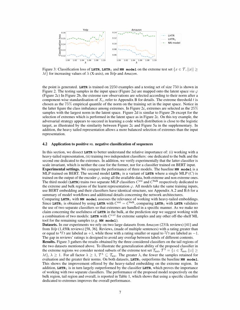
Figure 3: Classification loss of LHTR, LHTR1 and NN model on the extreme test set {x ∈ T , ||x|| ≥λt} for increasing values of λ (X-axis), on Yelp and Amazon.

the point is generated. LHTR is trained on 2250 examples and a testing set of size 750 is shown inFigure 2. The testing samples in the input space (Figure 2a) are mapped onto the latent space via ϕ(Figure 2c) In Figure 2b, the extreme raw observations are selected according to their norm after acomponent-wise standardisation of Xi, refer to Appendix B for details. The extreme threshold t ischosen as the 75% empirical quantile of the norm on the training set in the input space. Notice inthe latter figure the class imbalance among extremes. In Figure 2c, extremes are selected as the 25%samples with the largest norm in the latent space. Figure 2d is similar to Figure 2b except for theselection of extremes which is performed in the latent space as in Figure 2c. On this toy example, theadversarial strategy appears to succeed in learning a code which distribution is close to the logistictarget, as illustrated by the similarity between Figure 2c and Figure 5a in the supplementary. Inaddition, the heavy tailed representation allows a more balanced selection of extremes than the inputrepresentation.

4.2 Application to positive vs. negative classification of sequences

In this section, we dissect LHTR to better understand the relative importance of: (i) working with aheavy-tailed representation, (ii) training two independent classifiers: one dedicated to the bulk and thesecond one dedicated to the extremes. In addition, we verify experimentally that the latter classifier isscale invariant, which is neither the case for the former, nor for a classifier trained on BERT input.Experimental settings. We compare the performance of three models. The baseline NN model is aMLP trained on BERT. The second model LHTR1 is a variant of LHTR where a single MLP (C) istrained on the output of the encoder ϕ, using all the available data, both extreme and non extreme ones.The third model (LHTR) trains two separate MLP classifiers Cext and Cbulk respectively dedicated tothe extreme and bulk regions of the learnt representation ϕ. All models take the same training inputs,use BERT embedding and their classifiers have identical structure, see Appendix A.2 and B.6 for asummary of model workflows and additional details concerning the network architectures.Comparing LHTR1 with NN model assesses the relevance of working with heavy-tailed embeddings.Since LHTR1 is obtained by using LHTR with Cext = Cbulk, comparing LHTR1 with LHTR validatesthe use of two separate classifiers so that extremes are handled in a specific manner. As we make noclaim concerning the usefulness of LHTR in the bulk, at the prediction step we suggest working witha combination of two models: LHTR with Cext for extreme samples and any other off-the-shelf MLtool for the remaining samples (e.g. NN model).Datasets. In our experiments we rely on two large datasets from Amazon (231k reviews) [41] andfrom Yelp (1,450k reviews) [58, 36]. Reviews, (made of multiple sentences) with a rating greater thanor equal to 4/ 5 are labeled as +1, while those with a rating smaller or equal to 2/ 5 are labeled as −1.The gap in reviews’ ratings is designed to avoid any overlap between labels of different contents.Results. Figure 3 gathers the results obtained by the three considered classifiers on the tail regions ofthe two datasets mentioned above. To illustrate the generalization ability of the proposed classifier inthe extreme regions we consider nested subsets of the extreme test set Ttest, T λ = {z ∈ Ttest, ‖z‖ ≥λt}, λ ≥ 1. For all factor λ ≥ 1, T λ ⊆ Ttest. The greater λ, the fewer the samples retained forevaluation and the greater their norms. On both datasets, LHTR1 outperforms the baseline NN model.This shows the improvement offered by the heavy-tailed embedding on the extreme region. Inaddition, LHTR1 is in turn largely outperformed by the classifier LHTR, which proves the importanceof working with two separate classifiers. The performance of the proposed model respectively on thebulk region, tail region and overall, is reported in Table 1, which shows that using a specific classifierdedicated to extremes improves the overall performance.

7

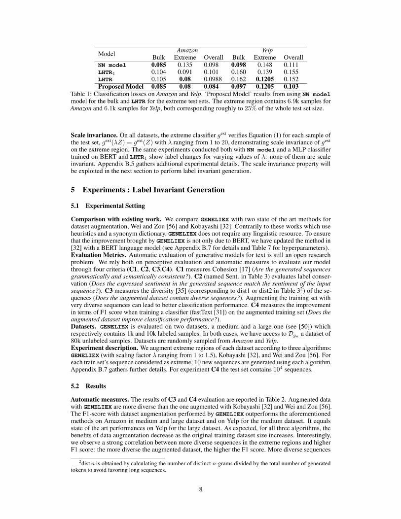
Model Amazon YelpBulk Extreme Overall Bulk Extreme Overall

NN model 0.085 0.135 0.098 0.098 0.148 0.111LHTR1 0.104 0.091 0.101 0.160 0.139 0.155LHTR 0.105 0.08 0.0988 0.162 0.1205 0.152Proposed Model 0.085 0.08 0.084 0.097 0.1205 0.103

Table 1: Classification losses on Amazon and Yelp. ‘Proposed Model’ results from using NN modelmodel for the bulk and LHTR for the extreme test sets. The extreme region contains 6.9k samples forAmazon and 6.1k samples for Yelp, both corresponding roughly to 25% of the whole test set size.

Scale invariance. On all datasets, the extreme classifier gext verifies Equation (1) for each sample ofthe test set, gext(λZ) = gext(Z) with λ ranging from 1 to 20, demonstrating scale invariance of gext

on the extreme region. The same experiments conducted both with NN model and a MLP classifiertrained on BERT and LHTR1 show label changes for varying values of λ: none of them are scaleinvariant. Appendix B.5 gathers additional experimental details. The scale invariance property willbe exploited in the next section to perform label invariant generation.

5 Experiments : Label Invariant Generation

5.1 Experimental Setting

Comparison with existing work. We compare GENELIEX with two state of the art methods fordataset augmentation, Wei and Zou [56] and Kobayashi [32]. Contrarily to these works which useheuristics and a synonym dictionary, GENELIEX does not require any linguistic resource. To ensurethat the improvement brought by GENELIEX is not only due to BERT, we have updated the method in[32] with a BERT language model (see Appendix B.7 for details and Table 7 for hyperparameters).Evaluation Metrics. Automatic evaluation of generative models for text is still an open researchproblem. We rely both on perceptive evaluation and automatic measures to evaluate our modelthrough four criteria (C1, C2, C3,C4). C1 measures Cohesion [17] (Are the generated sequencesgrammatically and semantically consistent?). C2 (named Sent. in Table 3) evaluates label conser-vation (Does the expressed sentiment in the generated sequence match the sentiment of the inputsequence?). C3 measures the diversity [35] (corresponding to dist1 or dist2 in Table 32) of the se-quences (Does the augmented dataset contain diverse sequences?). Augmenting the training set withvery diverse sequences can lead to better classification performance. C4 measures the improvementin terms of F1 score when training a classifier (fastText [31]) on the augmented training set (Does theaugmented dataset improve classification performance?).Datasets. GENELIEX is evaluated on two datasets, a medium and a large one (see [50]) whichrespectively contains 1k and 10k labeled samples. In both cases, we have access to Dgn a dataset of80k unlabeled samples. Datasets are randomly sampled from Amazon and Yelp.Experiment description. We augment extreme regions of each dataset according to three algorithms:GENELIEX (with scaling factor λ ranging from 1 to 1.5), Kobayashi [32], and Wei and Zou [56]. Foreach train set’s sequence considered as extreme, 10 new sequences are generated using each algorithm.Appendix B.7 gathers further details. For experiment C4 the test set contains 104 sequences.

5.2 Results

Automatic measures. The results of C3 and C4 evaluation are reported in Table 2. Augmented datawith GENELIEX are more diverse than the one augmented with Kobayashi [32] and Wei and Zou [56].The F1-score with dataset augmentation performed by GENELIEX outperforms the aforementionedmethods on Amazon in medium and large dataset and on Yelp for the medium dataset. It equalsstate of the art performances on Yelp for the large dataset. As expected, for all three algorithms, thebenefits of data augmentation decrease as the original training dataset size increases. Interestingly,we observe a strong correlation between more diverse sequences in the extreme regions and higherF1 score: the more diverse the augmented dataset, the higher the F1 score. More diverse sequences

2distn is obtained by calculating the number of distinct n-grams divided by the total number of generatedtokens to avoid favoring long sequences.

8

ModelAmazon Yelp

Medium Large Medium LargeF1 dist1/dist2 F1 dist1/dist2 F1 dist1/dist2 F1 dist1/dist2

Raw Data 84.0 X 93.3 X 86.7 X 94.1 XKobayashi [32] 85.0 0.10/0.47 92.9 0.14/0.53 87.0 0.15/0.53 94.0 0.14/0.58Wei and Zou [56] 85.2 0.11/0.50 93.2 0.14/0.54 87.0 0.15/0.52 94.2 0.16/0.59GENELIEX 86.3 0.14/0.52 94.0 0.18/0.58 88.4 0.18/0.62 94.2 0.16/0.60

Table 2: Quantitative Evaluation. Algorithms are compared according to C3 and C4. dist1 and dist2respectively stand for distinct 1 and 2, it measures the diversity of new sequences in terms of unigramsand bigrams. F1 is the F1-score for FastText classifier trained on an augmented labelled training set.

Model Amazon YelpSent. Cohesion Sent. Cohesion

Raw Data 83.6 78.3 80.6 0.71Kobayashi [32] 80.0 84.2 82.9 0.72Wei and Zou [56] 69.0 67.4 80.0 0.60GENELIEX 78.4 73.2 85.7 0.77

Table 3: Qualitative evaluation with three turkers. Sent. stands for sentiment label preservation.The Krippendorff Alpha for Amazon is α = 0.28 on the sentiment classification and α = 0.20 forcohesion. The Krippendorff Alpha for Yelp is α = 0.57 on the sentiment classification and α = 0.48for cohesion.

are thus more likely to lead to better improvement on downstream tasks (e.g. classification).Perceptive Measures. To evaluate C1, C2, three turkers were asked to annotate the cohesion andthe sentiment of 100 generated sequences for each algorithm and for the raw data. F1 scores ofthis evaluation are reported in Table 3. Grammar evaluation confirms the findings of [56] showingthat random swaps and deletions do not always maintain the cohesion of the sequence. In contrast,GENELIEX and Kobayashi [32], using vectorial representations, produce more coherent sequences.Concerning sentiment label preservation, on Yelp, GENELIEX achieves the highest score whichconfirms the observed improvement reported in Table 2. On Amazon, turker annotations with datafrom GENELIEX obtain a lower F1-score than from Kobayashi [32]. This does not correlate withresults in Table 2 and may be explained by a lower Krippendorff Alpha3 on Amazon (α = 0.20) thanon Yelp (α = 0.57).

6 Broader Impact

In this work, we propose a method resulting in heavy-tailed text embeddings. As we make noassumption on the nature of the input data, the suggested method is not limited to textual dataand can be extended to any type of modality (e.g. audio, video, images). A classifier, trained onaforementioned embedding is dilation invariant (see Equation 1) on the extreme region. A dilationinvariant classifier enables better generalization for new samples falling out of the training envelop.For critical application ranging from web content filtering (e.g. spam [27], hate speech detection [18],fake news [43]) to medical case reports to court decisions it is crucial to build classifiers with lowergeneralization error. The scale invariance property can also be exploited to automatically augmenta small dataset on its extreme region. For application where data collection requires a huge effortboth in time and cost (e.g. industrial factory design, classification for rare language [4]), beyondindustrial aspect, active learning problems involving heavy-tailed data may highly benefit from ourdata augmentation approach.

7 Acknowledgement

Anne Sabourin was partly supported by the Chaire Stress testing from Ecole Polytechnique and BNPParibas. Concerning Eric Gaussier, this project partly fits within the MIAI project (ANR-19-P3IA-0003).

3measure of inter-rater reliability in [0, 1]: 0 is perfect disagreement and 1 is perfect agreement.

9

References[1] Mastane Achab, Stephan Clemencon, Aurelien Garivier, Anne Sabourin, and Claire Vernade.

Max k-armed bandit: On the extremehunter algorithm and beyond. In Joint European Confer-ence on Machine Learning and Knowledge Discovery in Databases, pages 389–404. Springer,2017.

[2] R Harald Baayen. Word frequency distributions, volume 18. Springer Science & BusinessMedia, 2002.

[3] Rohit Babbar, Cornelia Metzig, Ioannis Partalas, Eric Gaussier, and Massih-Reza Amini. Onpower law distributions in large-scale taxonomies. ACM SIGKDD Explorations Newsletter, 16(1):47–56, 2014.

[4] M Saiful Bari, Muhammad Tasnim Mohiuddin, and Shafiq Joty. Multimix: A robust dataaugmentation strategy for cross-lingual nlp. arXiv preprint arXiv:2004.13240, 2020.

[5] Yoshua Bengio, Rejean Ducharme, Pascal Vincent, and Christian Jauvin. A neural probabilisticlanguage model. Journal of machine learning research, 3(Feb):1137–1155, 2003.

[6] A. Carpentier and M. Valko. Extreme bandits. In Advances in Neural Information ProcessingSystems 27, pages 1089–1097. Curran Associates, Inc., 2014.

[7] Emile Chapuis, Pierre Colombo, Matteo Manica, Matthieu Labeau, and Chloe Clavel. Hierar-chical pre-training for sequence labelling in spoken dialog. arXiv preprint arXiv:2009.11152,2020.

[8] Mael Chiapino and Anne Sabourin. Feature clustering for extreme events analysis, withapplication to extreme stream-flow data. In International Workshop on New Frontiers in MiningComplex Patterns, pages 132–147. Springer, 2016.

[9] Mael Chiapino, Stephan Clemencon, Vincent Feuillard, and Anne Sabourin. A multivariateextreme value theory approach to anomaly clustering and visualization. Computational Statistics,pages 1–22, 2019.

[10] Mael Chiapino, Anne Sabourin, and Johan Segers. Identifying groups of variables with thepotential of being large simultaneously. Extremes, 22(2):193–222, 2019.

[11] Kenneth W Church and William A Gale. Poisson mixtures. Natural Language Engineering, 1(2):163–190, 1995.

[12] D. A. Clifton, S. Hugueny, and L. Tarassenko. Novelty detection with multivariate extremevalue statistics. J Signal Process Syst., 65:371–389, 2011.

[13] Stephane Clinchant and Eric Gaussier. Information-based models for ad hoc ir. In Proceedingsof the 33rd international ACM SIGIR conference on Research and development in informationretrieval, pages 234–241, 2010.

[14] Stuart G Coles and Jonathan A Tawn. Statistical methods for multivariate extremes: anapplication to structural design. Journal of the Royal Statistical Society: Series C (AppliedStatistics), 43(1):1–31, 1994.

[15] Pierre Colombo, Wojciech Witon, Ashutosh Modi, James Kennedy, and Mubbasir Kapadia.Affect-driven dialog generation. arXiv preprint arXiv:1904.02793, 2019.

[16] Pierre Colombo, Emile Chapuis, Matteo Manica, Emmanuel Vignon, Giovanna Varni, andChloe Clavel. Guiding attention in sequence-to-sequence models for dialogue act prediction.arXiv preprint arXiv:2002.08801, 2020.

[17] Scott Crossley and Danielle McNamara. Cohesion, coherence, and expert evaluations of writingproficiency. In Proceedings of the Annual Meeting of the Cognitive Science Society, volume 32(32), 2010.

10

[18] Thomas Davidson, Dana Warmsley, Michael Macy, and Ingmar Weber. Automated hate speechdetection and the problem of offensive language. In Eleventh international aaai conference onweb and social media, 2017.

[19] Jacob Devlin, Ming-Wei Chang, Kenton Lee, and Kristina Toutanova. Bert: Pre-training ofdeep bidirectional transformers for language understanding. arXiv preprint arXiv:1810.04805,2018.

[20] Tanvi Dinkar, Pierre Colombo, Matthieu Labeau, and Chloe Clavel. The importance of fillersfor text representations of speech transcripts. arXiv preprint arXiv:2009.11340, 2020.

[21] Maziar Moradi Fard, Thibaut Thonet, and Eric Gaussier. Deep k-means: Jointly clustering withk-means and learning representations. arXiv preprint arXiv:1806.10069, 2018.

[22] N. Goix, A. Sabourin, and S. Clemencon. Learning the dependence structure of rare events: anon-asymptotic study. In Conference on Learning Theory, pages 843–860, 2015.

[23] N. Goix, A. Sabourin, and S. Clemencon. Sparse representation of multivariate extremes withapplications to anomaly ranking. In Artificial Intelligence and Statistics, pages 75–83, 2016.

[24] N. Goix, A. Sabourin, and S. Clemencon. Sparse representation of multivariate extremes withapplications to anomaly detection. Journal of Multivariate Analysis, 161:12–31, 2017.

[25] Ian Goodfellow, Jean Pouget-Abadie, Mehdi Mirza, Bing Xu, David Warde-Farley, SherjilOzair, Aaron Courville, and Yoshua Bengio. Generative adversarial nets. In Advances in neuralinformation processing systems, pages 2672–2680, 2014.

[26] Ian Goodfellow, Yoshua Bengio, and Aaron Courville. Deep Learning. MIT Press, 2016.http://www.deeplearningbook.org.

[27] Thiago S Guzella and Walmir M Caminhas. A review of machine learning approaches to spamfiltering. Expert Systems with Applications, 36(7):10206–10222, 2009.

[28] Ari Holtzman, Jan Buys, Maxwell Forbes, and Yejin Choi. The curious case of neural textdegeneration. arXiv preprint arXiv:1904.09751, 2019.

[29] Hamid Jalalzai and Remi Leluc. Informative clusters for multivariate extremes. arXiv preprintarXiv:2008.07365, 2020.

[30] Hamid Jalalzai, Stephan Clemencon, and Anne Sabourin. On binary classification in extremeregions. In Advances in Neural Information Processing Systems, pages 3092–3100, 2018.

[31] Armand Joulin, Edouard Grave, Piotr Bojanowski, and Tomas Mikolov. Bag of tricks forefficient text classification. arXiv preprint arXiv:1607.01759, 2016.

[32] Sosuke Kobayashi. Contextual augmentation: Data augmentation by words with paradigmaticrelations. arXiv preprint arXiv:1805.06201, 2018.

[33] Dimitrios Kotzias, Misha Denil, Nando De Freitas, and Padhraic Smyth. From group toindividual labels using deep features. In Proceedings of the 21th ACM SIGKDD InternationalConference on Knowledge Discovery and Data Mining, pages 597–606. ACM, 2015.

[34] Pierre Laforgue, Stephan Clemencon, and Florence d’Alche Buc. Autoencoding any datathrough kernel autoencoders. arXiv preprint arXiv:1805.11028, 2018.

[35] Jiwei Li, Michel Galley, Chris Brockett, Jianfeng Gao, and Bill Dolan. A diversity-promotingobjective function for neural conversation models. arXiv preprint arXiv:1510.03055, 2015.

[36] Jialu Liu, Jingbo Shang, Chi Wang, Xiang Ren, and Jiawei Han. Mining quality phrases frommassive text corpora. In Proceedings of the 2015 ACM SIGMOD International Conference onManagement of Data, pages 1729–1744. ACM, 2015.

[37] Ilya Loshchilov and Frank Hutter. Decoupled weight decay regularization. arXiv preprintarXiv:1711.05101, 2017.

11

[38] Rasmus E Madsen, David Kauchak, and Charles Elkan. Modeling word burstiness using thedirichlet distribution. In Proceedings of the 22nd international conference on Machine learning,pages 545–552, 2005.

[39] Alireza Makhzani, Jonathon Shlens, Navdeep Jaitly, Ian Goodfellow, and Brendan Frey. Adver-sarial autoencoders. arXiv preprint arXiv:1511.05644, 2015.

[40] Benoit Mandelbrot. An informational theory of the statistical structure of language. Communi-cation theory, 84:486–502, 1953.

[41] Julian McAuley and Jure Leskovec. Hidden factors and hidden topics: understanding ratingdimensions with review text. In Proceedings of the 7th ACM conference on Recommendersystems, pages 165–172. ACM, 2013.

[42] George A Miller. Wordnet: a lexical database for english. Communications of the ACM, 38(11):39–41, 1995.

[43] Veronica Perez-Rosas, Bennett Kleinberg, Alexandra Lefevre, and Rada Mihalcea. Automaticdetection of fake news. arXiv preprint arXiv:1708.07104, 2017.

[44] Matthew E. Peters, Mark Neumann, Mohit Iyyer, Matt Gardner, Christopher Clark, Kenton Lee,and Luke Zettlemoyer. Deep contextualized word representations. In Proc. of NAACL, 2018.

[45] Alec Radford, Karthik Narasimhan, Tim Salimans, and Ilya Sutskever. Improving languageunderstanding by generative pre-training. URL https://s3-us-west-2. amazonaws. com/openai-assets/researchcovers/languageunsupervised/language understanding paper. pdf, 2018.

[46] Alexander J Ratner, Henry Ehrenberg, Zeshan Hussain, Jared Dunnmon, and Christopher Re.Learning to compose domain-specific transformations for data augmentation. In Advances inneural information processing systems, pages 3236–3246, 2017.

[47] Sidney I Resnick. Extreme values, regular variation and point processes. Springer, 2013.

[48] S.J. Roberts. Novelty detection using extreme value statistics. IEE P-VIS IMAGE SIGN, 146:124–129, Jun 1999.

[49] S.J Roberts. Extreme value statistics for novelty detection in biomedical data processing. IEEP-SCI MEAS TECH, 147:363–367, 2000.

[50] Miikka Silfverberg, Adam Wiemerslage, Ling Liu, and Lingshuang Jack Mao. Data augmenta-tion for morphological reinflection. Proceedings of the CoNLL SIGMORPHON 2017 SharedTask: Universal Morphological Reinflection, pages 90–99, 2017.

[51] A. Stephenson. Simulating multivariate extreme value distributions of logistic type. Extremes,6(1):49–59, 2003.

[52] Ilya Sutskever, Oriol Vinyals, and Quoc V Le. Sequence to sequence learning with neuralnetworks. In Advances in neural information processing systems, pages 3104–3112, 2014.

[53] Albert Thomas, Stephan Clemencon, Alexandre Gramfort, and Anne Sabourin. Anomalydetection in extreme regions via empirical mv-sets on the sphere. In AISTATS, pages 1011–1019,2017.

[54] Ashish Vaswani, Noam Shazeer, Niki Parmar, Jakob Uszkoreit, Llion Jones, Aidan N Gomez,Łukasz Kaiser, and Illia Polosukhin. Attention is all you need. In Advances in neural informationprocessing systems, pages 5998–6008, 2017.

[55] Jason Wang and Luis Perez. The effectiveness of data augmentation in image classificationusing deep learning. Convolutional Neural Networks Vis. Recognit, 2017.

[56] Jason Wei and Kai Zou. Eda: Easy data augmentation techniques for boosting performanceon text classification tasks. In Proceedings of the 2019 Conference on Empirical Methods inNatural Language Processing and the 9th International Joint Conference on Natural LanguageProcessing (EMNLP-IJCNLP), pages 6383–6389, 2019.

12

[57] Wojciech Witon, Pierre Colombo, Ashutosh Modi, and Mubbasir Kapadia. Disney at iest 2018:Predicting emotions using an ensemble. In Proceedings of the 9th Workshop on ComputationalApproaches to Subjectivity, Sentiment and Social Media Analysis, pages 248–253, 2018.

[58] Xiao Yu, Xiang Ren, Yizhou Sun, Quanquan Gu, Bradley Sturt, Urvashi Khandelwal, BrandonNorick, and Jiawei Han. Personalized entity recommendation: A heterogeneous informationnetwork approach. In Proceedings of the 7th ACM international conference on Web search anddata mining, pages 283–292. ACM, 2014.

13