arX

iv:h

ep-p

h/01

1029

2v1

23

Oct

200

1

DO-TH 2001/17

hep-ph/0110292

October 2001

Heavy Quark Production in CC and NC DISand

The Structure of Real and Virtual Photonsin NLO QCD

Dissertation

zur Erlangung des Grades eines

Doktors der Naturwissenschaften

der Abteilung Physik

der Universitat Dortmund

vorgelegt von

Ingo Jan Schienbein

Juli 2001

Fur meinen Vater

Granger stood looking back with Montag. “Everyone must leave something behind when he

dies, my grandfather said. A child or a book or a painting or a house or a wall built or a

pair of shoes made. Or a garden planted. Something your hand touched some way so your

soul has somewhere to go when you die, and when people look at that tree or that flower you

planted, you’re there. It doesn’t matter what you do, he said, so long as you change something

from the way it was before you touched it into something that’s like you after you take your

hands away. The difference between the man who just cuts lawns and a real gardener is in the

touching, he said. The lawn–cutter might just as well not have been there at all; the gardener

will be there a life–time.”

Ray Bradbury, Fahrenheit 451

Contents

I Heavy Quark Production in CC and NC DIS 1

1 Introduction and Survey 2

2 Charged Current Leptoproduction of D–Mesons in the Variable Flavor

Scheme 5

2.1 Introduction . . . . . . . . . . . . . . . . . . . . . . . . . . . . . . . . . . . 5

2.2 Gluon–Fusion . . . . . . . . . . . . . . . . . . . . . . . . . . . . . . . . . . 6

2.3 CC Leptoproduction within ACOT . . . . . . . . . . . . . . . . . . . . . . 8

2.4 Numerical Results . . . . . . . . . . . . . . . . . . . . . . . . . . . . . . . . 9

2.5 Summary . . . . . . . . . . . . . . . . . . . . . . . . . . . . . . . . . . . . 10

3 Quark Masses in Deep Inelastic Structure Functions 12

3.1 Introduction . . . . . . . . . . . . . . . . . . . . . . . . . . . . . . . . . . . 12

3.2 Heavy Quark Contributions to ACOT Structure Functions . . . . . . . . . 14

3.2.1 DIS on a Massive Quark at O(α0s) . . . . . . . . . . . . . . . . . . . 14

3.2.2 DIS on a Massive Quark at O(α1s) . . . . . . . . . . . . . . . . . . . 17

3.2.3 Gluon Fusion Contributions at O(α1s) . . . . . . . . . . . . . . . . . 19

3.2.4 ACOT Structure Functions at O(α1s) . . . . . . . . . . . . . . . . . 20

3.3 Results for NC and CC Structure Functions . . . . . . . . . . . . . . . . . 21

3.3.1 NC Structure Functions . . . . . . . . . . . . . . . . . . . . . . . . 21

3.3.2 CC Structure Functions . . . . . . . . . . . . . . . . . . . . . . . . 25

CONTENTS ii

3.4 Conclusions . . . . . . . . . . . . . . . . . . . . . . . . . . . . . . . . . . . 28

4 Charm Fragmentation in Deep Inelastic Scattering 29

4.1 Introduction . . . . . . . . . . . . . . . . . . . . . . . . . . . . . . . . . . . 29

4.2 Semi–Inclusive Heavy Quark Structure Functions . . . . . . . . . . . . . . 31

4.2.1 Scattering on Massive Quarks . . . . . . . . . . . . . . . . . . . . . 31

4.2.2 Gluon Fusion Contributions at O(α1s) . . . . . . . . . . . . . . . . . 34

4.2.3 Subtraction Terms . . . . . . . . . . . . . . . . . . . . . . . . . . . 34

4.2.4 SI Structure Functions at O(α1s) . . . . . . . . . . . . . . . . . . . . 36

4.3 The Charm Fragmentation Function in SI DIS . . . . . . . . . . . . . . . . 37

4.3.1 CC DIS . . . . . . . . . . . . . . . . . . . . . . . . . . . . . . . . . 37

4.3.2 NC DIS . . . . . . . . . . . . . . . . . . . . . . . . . . . . . . . . . 42

4.4 Conclusions . . . . . . . . . . . . . . . . . . . . . . . . . . . . . . . . . . . 45

5 Summary 47

II The Structure of Real and Virtual Photons 49

6 Introduction and Survey 50

7 Photon–Photon Scattering 54

7.1 Kinematics . . . . . . . . . . . . . . . . . . . . . . . . . . . . . . . . . . . 55

7.1.1 The Hadronic Tensor W µ′ν′,µν . . . . . . . . . . . . . . . . . . . . . 57

7.1.2 Derivation of the Cross Section . . . . . . . . . . . . . . . . . . . . 60

7.2 Photon Structure Functions . . . . . . . . . . . . . . . . . . . . . . . . . . 61

7.2.1 Structure Functions for a Spin–Averaged Photon . . . . . . . . . . 62

7.2.2 Longitudinal and Transverse Target Photons . . . . . . . . . . . . . 63

7.3 QED–Factorization . . . . . . . . . . . . . . . . . . . . . . . . . . . . . . . 64

CONTENTS iii

8 The Doubly Virtual Box in LO 71

8.1 Unintegrated Structure Functions . . . . . . . . . . . . . . . . . . . . . . . 72

8.2 Inclusive Structure Functions . . . . . . . . . . . . . . . . . . . . . . . . . 75

8.3 Comparison with Present e+e− Virtual Photon Data . . . . . . . . . . . . 77

9 The Partonic Structure of Real and Virtual Photons: Theoretical

Framework 82

9.1 Introduction . . . . . . . . . . . . . . . . . . . . . . . . . . . . . . . . . . . 82

9.2 Photon Structure Functions in the QCD–Improved Parton Model . . . . . 85

9.2.1 Scheme Choice . . . . . . . . . . . . . . . . . . . . . . . . . . . . . 86

9.2.2 Heavy Flavor Contributions . . . . . . . . . . . . . . . . . . . . . . 87

9.3 Q2–Evolution . . . . . . . . . . . . . . . . . . . . . . . . . . . . . . . . . . 89

9.3.1 Evolution Equations . . . . . . . . . . . . . . . . . . . . . . . . . . 89

9.3.2 Analytic Solutions . . . . . . . . . . . . . . . . . . . . . . . . . . . 92

9.3.3 Numerical Mellin–Inversion . . . . . . . . . . . . . . . . . . . . . . 94

9.3.4 Boundary Conditions for a Deeply Virtual Target Photon . . . . . . 94

9.3.5 Momentum Sum . . . . . . . . . . . . . . . . . . . . . . . . . . . . 98

9.4 Longitudinal Target Photons . . . . . . . . . . . . . . . . . . . . . . . . . . 100

10 Pionic Parton Densities in a Constituent Quark Model 102

11 Radiatively Generated Parton Distributions of Real and Virtual Pho-

tons 109

11.1 Introduction . . . . . . . . . . . . . . . . . . . . . . . . . . . . . . . . . . . 109

11.2 The Parton Content of Real Photons . . . . . . . . . . . . . . . . . . . . . 111

11.2.1 Boundary Conditions . . . . . . . . . . . . . . . . . . . . . . . . . . 111

11.2.2 Quantitative Results . . . . . . . . . . . . . . . . . . . . . . . . . . 113

11.3 The Photon Structure Function at Small–x . . . . . . . . . . . . . . . . . . 118

CONTENTS iv

11.4 The Parton Content of Virtual Photons . . . . . . . . . . . . . . . . . . . . 123

11.4.1 Boundary Conditions . . . . . . . . . . . . . . . . . . . . . . . . . . 123

11.4.2 Quantitative Results . . . . . . . . . . . . . . . . . . . . . . . . . . 125

11.5 Summary and Conclusions . . . . . . . . . . . . . . . . . . . . . . . . . . . 131

12 Has the QCD RG–Improved Parton Content of Virtual Photons been

Observed? 133

12.1 Introduction . . . . . . . . . . . . . . . . . . . . . . . . . . . . . . . . . . . 133

12.2 RG–Improved Parton Model Expectations for the Effective Structure Func-

tion Feff . . . . . . . . . . . . . . . . . . . . . . . . . . . . . . . . . . . . . 134

12.3 Comparison with DIS ep Data and Effective Quark Distributions . . . . . . 137

12.4 Possible Signatures for the QCD Parton Content of Virtual Photons . . . . 140

12.5 Summary and Conclusions . . . . . . . . . . . . . . . . . . . . . . . . . . . 143

13 Summary 144

A Deep Inelastic Scattering on Massive Quarks at O(α1s) 147

A.1 Real Gluon Emission . . . . . . . . . . . . . . . . . . . . . . . . . . . . . . 147

A.2 Vertex Correction . . . . . . . . . . . . . . . . . . . . . . . . . . . . . . . . 149

A.2.1 Results . . . . . . . . . . . . . . . . . . . . . . . . . . . . . . . . . . 149

A.2.2 Calculation . . . . . . . . . . . . . . . . . . . . . . . . . . . . . . . 151

A.3 Real and Virtual Contributions to Structure Functions . . . . . . . . . . . 156

A.4 Comparison with E. Hoffmann and R. Moore, Z. Phys. C20, 71 (1983) . . 158

B Matrix Elements for Real Gluon Emission off Massive Quarks 161

C Limits of the Doubly Virtual Box 163

C.1 General Bjorken Limit: m2, P 2 ≪ Q2 . . . . . . . . . . . . . . . . . . . . . 165

C.2 m2 = 0, P 2 ≪ Q2 . . . . . . . . . . . . . . . . . . . . . . . . . . . . . . . . 165

CONTENTS v

C.3 Real Photon Limit: P 2 = 0 . . . . . . . . . . . . . . . . . . . . . . . . . . . 166

D Parametrizations 168

D.1 Pion Distributions . . . . . . . . . . . . . . . . . . . . . . . . . . . . . . . 168

D.1.1 Parametrization of LO Parton Distributions . . . . . . . . . . . . . 168

D.1.2 Parametrization of NLO(MS) Parton Distributions . . . . . . . . . 170

D.2 Photon Distributions . . . . . . . . . . . . . . . . . . . . . . . . . . . . . . 171

D.2.1 Parametrization of LO ‘pointlike’ Photonic Parton Distributions . . 171

D.2.2 Parametrization of NLO ‘pointlike’ Photonic Parton Distributions . 173

Preface

This thesis has been divided into two parts both being applications of perturbative Quan-

tum Chromo Dynamics (QCD).

The first part ’Heavy Quark Production in CC and NC DIS’ is a continuation of work

presented in [1] and has been done in collaboration with S. Kretzer. Part I is based on

the following publications [2–4]:

• S. Kretzer and I. Schienbein, Charged–current leptoproduction of D mesons in the

variable flavor scheme, Phys. Rev. D56, 1804 (1997) [Chapter 2].

• S. Kretzer and I. Schienbein, Heavy quark initiated contributions to deep inelastic

structure functions, Phys. Rev. D58, 094035 (1998) [Chapter 3].

• S. Kretzer and I. Schienbein, Heavy quark fragmentation in deep inelastic scattering,

Phys. Rev. D59, 054004 (1999) [Chapter 4].

The second part ’The Structure of Real and Virtual Photons’ has emerged from a

collaboration with Prof. M. Gluck and Prof. E. Reya. Part II is based on the following

publications [5–8]:

• M. Gluck, E. Reya, and I. Schienbein, Pionic parton distributions revisited, Eur.

Phys. J. C10, 313 (1999) [Chapter 10].

• M. Gluck, E. Reya, and I. Schienbein, Radiatively generated parton distributions for

real and virtual photons, Phys. Rev. D60, 054019 (1999); (E) D62 019902 (2000)

[Chapter 11].

• M. Gluck, E. Reya, and I. Schienbein, The Photon Structure Function at small–x,

Phys. Rev. D64, 017501 (2001) [Chapter 11].

CONTENTS vii

• M. Gluck, E. Reya, and I. Schienbein, Has the QCD RG–improved parton content

of virtual photons been observed?, Phys. Rev. D63, 074008 (2001) [Chapter 12].

The results of Refs. [5, 6] have also been summarized in [9, 10]. The work in Section 7.3

is completely new and has been done in collaboration with C. Sieg.

Part I

Heavy Quark Production in CC andNC DIS

Chapter 1

Introduction and Survey

Part I of this thesis is devoted to heavy quark production in charged current (CC) and

neutral current (NC) deep inelastic scattering (DIS) where a quark h with mass mh

is viewed as heavy if mh ≫ ΛQCD contrary to the light u, d, s quarks with mu,d,s ≪ΛQCD. Thus, the heavy quark mass provides a hard scale allowing for a perturbative

analysis. In deep inelastic heavy quark production a second hard scale is given by the

virtuality Q2 of the probing boson (photon, Z–boson, W–boson) such that we have to deal

with the theoretically interesting problem of describing a two–hard–scale process within

perturbative QCD (pQCD). In the following, we will prominently deal with charm quarks

being the lightest of the heavy quarks (h = c, b, t) in the standard model.

In addition to these general theoretical arguments, there are several important phe-

nomenological reasons for studying heavy quark production in DIS:

• Charm contributes up to 30% to the total structure function F p2 at small Bjorken–x

as measurements at the ep collider HERA at DESY have shown [11–13]. For this

reason a proper treatment of charm contributions in DIS is essential for a global

analysis of structure function data and a precise extraction of the parton densities

in the proton.

• NC charm production offers the possibility to extract the gluon distribution in the

proton from a measurement of F c2 [14, 15].

• CC charm production is sensitive to the nucleon’s strange sea. The momentum

(z) distributions of D–mesons from the fragmentation of charm quarks produced in

neutrino deep inelastic scattering have been used recently to determine the strange

3

quark distribution of the nucleon s(x,Q2) at leading order (LO) [16] and next–to–

leading order (NLO) [17].

In the past few years considerable effort has been devoted to including heavy quark

effects in DIS. If one could sum the whole perturbation series (keeping the full mass

dependence) one would arrive at unique perturbative QCD predictions. However, at any

finite order in perturbation theory differences arise due to distinct prescriptions (schemes)

[18–25] of how to order terms in the perturbative expansion. These schemes, in turn, enter

global analyses of parton distributions [26–28] and hence feed back on the resulting light

parton distributions [28]. It is therefore necessary to work out the various schemes as

much as possible and to compare them since a most complete possible understanding or

–even better– reduction of the theoretical uncertainties is required to make concise tests

of pQCD predictions against heavy flavor tagged deep inelastic data.

In this thesis we concentrate on the ACOT variable flavor number scheme (VFNS)

[19, 20] which we work out to full order O(α1s). Recently, this scheme has been proven

by Collins [21] to work at all orders of QCD factorization theory. We will perform all

required calculations with general couplings and masses in order to be able to describe

both CC and NC processes in one framework.

The outline of Part I will be as follows:

• In Chapter 2 we present formulae for the momentum (z) distributions of D–mesons

produced in neutrino deep inelastic scattering off strange partons. The expressions

are derived within the variable flavor scheme of Aivazis et al. (ACOT scheme) [20],

which is extended from its fully inclusive formulation to one–hadron inclusive lep-

toproduction. The dependence of the results on the assumed strange quark mass

ms is investigated and the ms → 0 limit is compared to the corresponding MS re-

sults. The importance of O(αs) quark–initiated corrections is demonstrated for the

ms = 0 case.

• In Chapter 3 we perform an explicit calculation of the before missing O(α1s) correc-

tions to deep inelastic scattering amplitudes on massive quarks within the ACOT

scheme using general masses and couplings thereby completing the ACOT formalism

up to full O(αs). After identifying the correct subtraction term the convergence of

these contributions towards the analogous coefficient functions for massless quarks,

4

obtained within the modified minimal subtraction scheme (MS), is demonstrated.

Furthermore, the importance of these contributions to neutral current and charged

current structure functions is investigated for several choices of the mass factoriza-

tion scale µ as well as the relevance of mass corrections.

• In Chapter 4 we turn to an analysis of semi–inclusive production of charm (mo-

mentum (z) distributions of D–mesons) in neutral current and charged current deep

inelastic scattering at full O(α1s). For this purpose we generalize the results of Chap-

ter 3 from its fully inclusive formulation to one–hadron inclusive leptoproduction.

We review the relevant massive formulae and subtraction terms and discuss their

massless limits. We show how the charm fragmentation function can be measured in

CC DIS and we investigate whether the charm production dynamics may be tested

in NC DIS. Furthermore, we also discuss finite initial state quark mass effects in

CC and NC DIS.

• Finally, we summarize our main results in Chapter 5. Some details of the calculation

and lengthy formulae are relegated to the Appendices A and B.

Chapter 2

Charged Current Leptoproduction ofD–Mesons in the Variable FlavorScheme

2.1 Introduction

The momentum (z) distributions of D–mesons from the fragmentation of charm quarks

produced in neutrino deep inelastic scattering (DIS) have been used recently to deter-

mine the strange quark distribution of the nucleon s(x,Q2) at leading order (LO) [16]

and next–to–leading order (NLO) [17]. A proper QCD calculation of this quantity re-

quires the convolution of a perturbative hard scattering charm production cross section

with a nonperturbative c → D fragmentation function Dc(z) leading at O(αs) to the

breaking of factorization in Bjorken–x and z as is well known for light quarks [29, 30].

So far experimental analyses have assumed a factorized cross section even at NLO [17].

This shortcoming has been pointed out in [31] and the hard scattering convolution kernels

needed for a correct NLO analysis have been calculated there in the MS scheme with three

massless flavors (u, d, s) using dimensional regularization. In the experimental NLO anal-

ysis in [17] the variable flavor scheme (VFS) of Aivazis, Collins, Olness and Tung (ACOT)

[20] for heavy flavor leptoproduction has been utilized. In this formalism one considers,

in addition to the quark scattering (QS) process, e.g. W+s → c, the contribution from

the gluon fusion (GF) process W+g → cs with its full ms–dependence. The collinear

logarithm which is already contained in the renormalized s(x,Q2) is subtracted off nu-

merically. The quark–initiated contributions from the subprocess W+s → cg (together

2.2 Gluon–Fusion 6

with virtual corrections) which were included in the complete NLO (MS) analysis in [31]

are usually neglected in the ACOT formalism. The ACOT formalism has been formu-

lated explicitly only for fully inclusive leptoproduction [20]. It is the main purpose here

to fill the gap and provide the expressions needed for a correct calculation of one–hadron

(D–meson) inclusive leptoproduction also in this formalism.

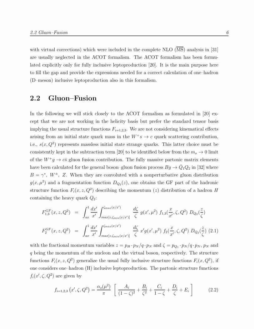
2.2 Gluon–Fusion

In the following we will stick closely to the ACOT formalism as formulated in [20] ex-

cept that we are not working in the helicity basis but prefer the standard tensor basis

implying the usual structure functions Fi=1,2,3. We are not considering kinematical effects

arising from an initial state quark mass in the W+s → c quark scattering contribution,

i.e., s(x,Q2) represents massless initial state strange quarks. This latter choice must be

consistently kept in the subtraction term [20] to be identified below from the ms → 0 limit

of the W+g → cs gluon fusion contribution. The fully massive partonic matrix elements

have been calculated for the general boson–gluon fusion process Bg → Q1Q2 in [32] where

B = γ∗, W±, Z. When they are convoluted with a nonperturbative gluon distribution

g(x, µ2) and a fragmentation function DQ2(z), one obtains the GF part of the hadronic

structure function Fi(x, z, Q2) describing the momentum (z) distribution of a hadron H

containing the heavy quark Q2:

FGF1,3 (x, z, Q2) =

∫ 1

ax

dx′

x′

∫ ζmax(x/x′)

max[z,ζmin(x/x′)]

dζ

ζg(x′, µ2) f1,3(

x

x′ , ζ, Q2) DQ2(

z

ζ)

FGF2 (x, z, Q2) =

∫ 1

ax

dx′

x′

∫ ζmax(x/x′)

max[z,ζmin(x/x′)]

dζ

ζx′g(x′, µ2) f2(

x

x′ , ζ, Q2) DQ2(

z

ζ) (2.1)

with the fractional momentum variables z = pH ·pN/q ·pN and ζ = pQ1 ·pN/q ·pN , pN and

q being the momentum of the nucleon and the virtual boson, respectively. The structure

functions Fi(x, z, Q2) generalize the usual fully inclusive structure functions Fi(x,Q

2), if

one considers one–hadron (H) inclusive leptoproduction. The partonic structure functions

fi(x′, ζ, Q2) are given by

fi=1,2,3

(x′, ζ, Q2

)=

αs(µ2)

π

[Ai

(1− ζ)2+

Bi

ζ2+

Ci

1− ζ+

Di

ζ+ Ei

](2.2)

2.2 Gluon–Fusion 7

with

A1

(x′, Q2

)= q+

x′2

4

m21

Q2

(1 +

∆m2

Q2− q−

q+

2m1m2

Q2

)

C1

(x′, Q2

)=

q+4

[1

2− x′(1− x′)− ∆m2 x′

Q2(1− 2x′) +

(∆m2 x′

Q2

)2

+q−q+

m1m2

Q22x′ (1− x′ − x′ m

21 +m2

2

Q2)

]

E1

(x′, Q2

)=

q+4

( −1 + 2x′ − 2x′2 )

A2

(x′, Q2

)= q+ x′

[x′2 m2

1

Q2

(1

2

(∆m2

Q2

)2

+∆m2 −m2

1

Q2+

1

2

)]

C2

(x′, Q2

)= q+

x′

4

[1− 2x′(1− x′) +

m21

Q2

(1 + 8x′ − 18x′2

)

+m2

2

Q2

(1− 4x′ + 6x′2

)− m4

1 +m42

Q42x′(1− 3x′) +

m21m

22

Q44x′(1− 5x′)

+∆m4 ∆m2

Q62x′2 − q−

q+

2m1m2

Q2

]

E2

(x′, Q2

)= q+ x′

[−1

2+ 3x′(1− x′)

]

A3

(x′, Q2

)= Rq m2

1 x′2 ∆m2 +Q2

Q4

C3

(x′, Q2

)= Rq

[1

2− x′(1− x′)− ∆m2

Q2x′(1− 2x′) +

∆m4

Q4x′2]

E3

(x′, Q2

)= 0

Bi= 1,23

(x′, Q2

)= ±Ai

(x′, Q2

)[m1 ↔ m2]

Di= 1,23

(x′, Q2

)= ±C3

(x′, Q2

)[m1 ↔ m2]

where ∆mn ≡ mn2 −mn

1 , m1,2 being the mass of the heavy quark Q1,2. The kinematical

boundaries of phase space in the convolutions in Eq. (2.1) are

ax =

[1 +

(m1 +m2)2

Q2

]x , ζmin,max(x

′) =1

2

[1 +

∆m2

Q2

x′

1− x′ ± vv

](2.3)

with v2 = 1 − (m1 +m2)2

Q2

x′

1− x′ , v2 = 1 − (m1 −m2)2

Q2

x′

1− x′ . The vector (V )

and axialvector (A) couplings of the γµ(V − Aγ5) quark current enter via q± = V 2 ± A2,

Rq = V A. 1 If the partonic structure functions in Eq. (2.2) are integrated over ζ the well1For the γ∗Z interference term the couplings read: q± = V γV Z ±AγAZ , Rq = 1/2(V γAZ + V ZAγ).

2.3 CC Leptoproduction within ACOT 8

known inclusive structure functions [33–35] for heavy flavor production are recovered:

∫ ζmax(x′)

ζmin(x′)

dζ fi= 1,23(x′, ζ, Q2) = ±fi(x

′, Q2) , (2.4)

where the fi(x′, Q2) can be found in [33].

2.3 CC Leptoproduction within ACOT

In the following we will consider the special case of charged current charm production,

i.e., m1 = ms, m2 = mc (q± = 2, 0; Rq = 1 assuming a vanishing Cabibbo angle). Of

course, all formulae below can be trivially adjusted to the general case of Eqs. (2.1) and

(2.2). The ms → 0 limit of the partonic structure functions in Eq. (2.2) is obtained by

keeping terms up to O(m2s) in the Ai, Ci and in ζmax due to the singularity of the phase

space integration stemming from ζ → 1. One obtains

limms→0

π

αs

fi(x′, ζ, Q2) = ci H

gi (x′

λ, ζ,m2

s, λ)

= ci δ(1− ζ) P (0)qg (

x′

λ) ln

Q2 +m2c

m2s

+O(m0s) (2.5)

where P (0)qg (x′) =

1

2[x′2 + (1 − x′2)], λ = Q2/(Q2 + m2

c), c1 = 1/2, c2 = x′/λ, c3 = 1

and the Hgi are the dimensionally regularized MS (ms = 0) gluonic coefficient functions

obtained in [31]. The ci arise from different normalizations of the fi and the Hgi and are

such that the infrared–safe subtracted [see Sec. 2.4] convolutions in Eq. (2.1) converge

towards the corresponding ones in [31] as ms → 0 if one realizes that x′/λ = ξ′, x/λ =

ξ ≡ x(1 +m2c/Q

2). Taking also the limit mc → 0 in Eq. (2.5) gives –besides the collinear

logarithm already present in Eq. (2.5)– finite expressions which agree with the massless

results of [29, 30].

In the ACOT formalism the GF convolutions in Eq. (2.1) coexist with the Born level

quark scattering contributions FQSi (x, z, Q2) = ki s(ξ, µ

2) Dc(z), ki=1,2,3 = 1, 2ξ, 2. The

overlap between the QS and the GF contributions is removed by introducing a subtraction

term (SUB) [20] which is obtained from the massless limit in Eq. (2.5)

F SUBi = ki

αs(µ2)

2πln

µ2

m2s

[∫ 1

ξ

dx′

x′ g(x′, µ2) P (0)qg

(ξ

x′

)]Dc(z) . (2.6)

2.4 Numerical Results 9

The complete O(αs) structure functions for the z distribution of charmed hadrons (i.e.,

dominantly D–mesons) produced in charged current DIS are then given in the ACOT

formalism [20] by

FACOTi = FQS

i − F SUBi + FGF

i . (2.7)

It is worthwhile noting that general results for polarized partonic structure functions

analogous to the unpolarized ones in Eq. (2.2) have been obtained in [36] allowing for

a formulation of polarized one–hadron inclusive heavy flavor leptoproduction within the

ACOT scheme along the same lines.

2.4 Numerical Results

In Fig. 2.1 we show the structure function FACOT2 at experimentally relevant [16] values

of x and Q2 for several finite choices of ms together with the asymptotic ms → 0 limit.

For Dc we use a Peterson fragmentation function [37]

Dc(z) = N{z[1− z−1 − εc/(1− z)

]2}−1

(2.8)

with εc = 0.06 [38–40] normalized to∫ 1

0dzDc(z) = 1 and we employ the GRV94(HO)

parton distributions [41] with mc = 1.5 GeV. Our choice of the factorization scale is

µ2 = Q2+m2c which ensures that there is no large ln(Q2+m2

c)/µ2 present in the difference

GF-SUB. As can be seen from Fig. 2.1 the effects of a finite strange mass are small and

converge rapidly towards the massless MS limit provided ms . 200 MeV as is usually

assumed [17].

In Fig. 2.2 we show the effects of adding the quark–initiated O(αs) correction from

the process W+s → cg (together with virtual corrections) to the asymptotic (ms → 0)

FACOT2 , employing the CTEQ4(MS) densities [42] with mc = 1.6 GeV. The O(αs) quark

contribution is usually neglected in the ACOT formalism since it is assumed to be effec-

tively suppressed by one order of αs with respect to the gluon fusion contribution due

to s(x, µ2)/g(x, µ2) ≃ O(αs). To check this assumption for the quantity F2(x, z, Q2) we

show, besides the full result, the contributions from the distinct processes (using again

µ2 = Q2 +m2c). The W+g → cs contribution corresponds to GF-SUB in Eq. (2.7). The

quark–initiated O(αs) contribution has been calculated in the MS scheme according to [31]

which is consistent with the asymptotic gluon–initiated correction in the ACOT scheme

2.5 Summary 10

0.16

0.18

0.2

0.22

0.24

0.26

0.28

0.3

0.32

0.34

0.2 0.3 0.4 0.5 0.6 0.7 0.8

x = 0.015

Q2 = 2.4 GeV2

FAC

OT

2

(x,

z,Q

2 )

ms [MeV]

z

0100300500

x = 0.125

Q2 = 17.9 GeV2

FAC

OT

2

(x,

z,Q

2 )

z0.04

0.05

0.06

0.07

0.08

0.09

0.1

0.11

0.12

0.2 0.3 0.4 0.5 0.6 0.7 0.8

Figure 2.1: The structure function FACOT2 (x, z, Q2) as defined in Eq. (2.7) using the

GRV94(HO) parton densities [41] with mc = 1.5 GeV and a Peterson fragmentation function[37] with εc = 0.06. Several finite choices for ms are shown as well as the asymptotic ms → 0limit.

due to Eq. (2.5). It can be seen that the quark–initiated correction is comparable in size

to the gluon–initiated correction around the maximum of F2. Since most of the exper-

imentally measured D–mesons originate from this region the O(αs) quark contributions

should not be neglected in a complete NLO calculation.

2.5 Summary

To summarize we have given formulae which extend the ACOT scheme [20] for the lep-

toproduction of heavy quarks from its fully inclusive formulation to one–hadron inclusive

leptoproduction. We have applied this formulation to D–meson production in charged

current DIS and studied finite ms corrections to the asymptotic ms → 0 limit. The cor-

2.5 Summary 11

-0.4

-0.2

0

0.2

0.4

0.6

0 0.1 0.2 0.3 0.4 0.5 0.6 0.7 0.8 0.9 1

x = 0.015

Q2 = 2.4 GeV2

ms = 0

total

(W+ s → c)

(W+ g → c s– )

(W+ s → c g)

F 2(x,

z,Q

2 )

z

x = 0.125

Q2 = 17.9 GeV2

F 2(x,

z,Q

2 )

z-0.1

-0.05

0

0.05

0.1

0.15

0.2

0.25

0.3

0 0.1 0.2 0.3 0.4 0.5 0.6 0.7 0.8 0.9 1

Figure 2.2: The structure function F2(x, z, Q2) for charged current leptoproduction of D–

mesons at O(αs) for ms = 0 using the CTEQ4(MS) parton distributions [42] and a Petersonfragmentation function [37] with εc = 0.06. The full O(αs) result is shown as well as theindividual contributions from the distinct quark– and gluon–initiated processes.

rections turned out to be small for reasonable choices of ms . 200 MeV and we have

shown that the ms → 0 limit reproduces the dimensionally regularized MS (ms = 0)

gluonic coefficient functions [31]. Furthermore we have investigated the quark–initiated

O(αs) corrections for ms = 0 using the relevant MS fermionic coefficient functions [31].

The latter corrections turned out to be numerically important at experimentally relevant

values of x and Q2 [16] and should be included in a complete NLO calculation of charged

current leptoproduction of D–mesons. In the next chapter, the quark–initiated diagrams

will be calculated up to O(αs) in the ACOT scheme allowing to study finite ms effects

stemming from these contributions as has been done in this chapter for the O(αs) gluon

contributions.

Chapter 3

Quark Masses in Deep InelasticStructure Functions

In this chapter we consider heavy quark contributions to inclusive deep inelastic struc-

ture functions within the ACOT variable flavor number scheme to which we contribute

the calculation of the before missing Bremsstrahlung corrections (incl. virtual graphs)

off initial state massive quarks. The calculation exemplifies factorization with massive

quark–partons as has recently been proven to all orders in perturbation theory by Collins

[21]. After identifying the correct subtraction term the convergence of these contribu-

tions towards the analogous coefficient functions for massless quarks, obtained within

the modified minimal subtraction scheme (MS), is demonstrated. Furthermore, the phe-

nomenological relevance of the contributions to neutral current (NC) and charged current

(CC) structure functions is investigated for several choices of the factorization scale. The

results presented in this chapter are taken from Ref. [3].

3.1 Introduction

Leptoproduction of heavy quarks has become a subject of major interest in QCD phe-

nomenology both for experimental and theoretical reasons. Heavy quark contributions are

an important component of measured neutral current (NC) [11–13] and charged current

(CC) [43] deep inelastic (DI) structure functions at lower values of Bjorken–x, accessible to

present experiments. Charm tagging in NC and CC deep inelastic scattering (DIS) offers

the possibility to pin down the nucleon’s gluon [44] and strange sea [16, 17, 45, 46] density,

respectively, both of which are nearly unconstrained by global fits to inclusive DI data.

3.1 Introduction 13

Theoretically it is challenging to understand the production mechanism of heavy quarks

within perturbative QCD. The cleanest and most predictive method [18] of calculating

heavy quark contributions to structure functions seems to be fixed order perturbation

theory (FOPT) where heavy quarks are produced exclusively by operators built from

light quarks (u,d,s) and gluons (g) and no initial state heavy quark lines show up in any

Feynman diagram. Heavy quarks produced via FOPT are therefore also called ‘extrin-

sic’ since no contractions of heavy quark operators with the nucleon wavefunction are

considered (which in turn would be characteristic for ‘intrinsic’ heavy quarks). Besides

FOPT much effort has been spent on formulating variable flavor number schemes (VFNS)

[19, 20, 22–24] which aim at resumming the quasi–collinear logs [ln(Q2/m2); Q and m be-

ing the virtuality of the mediated gauge boson and the heavy quark mass, respectively]

arising at any order in FOPT. All these schemes have in common that extrinsic FOPT

induces the boundary condition [23, 47]

q(x,Q20 = m2) = 0 +O(α2

s) (3.1)

for an intrinsic heavy quark density, which then undergoes massless renormalization group

(RG) evolution. Apart from their theoretical formulation VFNS have to be well under-

stood phenomenologically for a comparison with FOPT and with heavy quark tagged DI

data. We will concentrate here on the scheme developed by Aivazis, Collins, Olness and

Tung (ACOT) [19–21]. In the ACOT scheme full dependence on the heavy quark mass

is kept in graphs containing heavy quark lines. This gives rise to the above mentioned

quasi–collinear logs as well as to power suppressed terms of O[(m2/Q2)k]. While the latter

give mass corrections to the massless, dimensionally regularized, standard coefficient func-

tions (e.g. in the MS scheme), the former are removed by numerical subtraction since the

collinear region of phase space is already contained in the RG evolution of the heavy quark

density. Up to now explicit expressions in this scheme exist for DIS on a heavy quark at

O(α0s) [19] as well as for the production of heavy quarks via virtual boson gluon fusion

(GF) at O(α1s) [20]. In Section 3.2 we will give expressions which complete the scheme

up to O(α1s) and calculate DIS on a heavy quark at first order in the strong coupling,

i.e. B∗Q1 → Q2g (incl. virtual corrections to B∗Q1 → Q2) with general couplings of the

virtual boson B∗ to the heavy quarks, keeping all dependence on the masses m1,2 of the

quarks Q1,2. It is unclear whether (heavy) quark scattering (QS) and GF at O(α1s) should

be considered on the same level in the perturbation series. Due to its extrinsic prehis-

3.2 Heavy Quark Contributions to ACOT Structure Functions 14

tory QS(1) (bracketed upper indices count powers1 of αs) includes a collinear subgraph of

GF(2), e.g. γ∗c → cg contains the part of γ∗g → ccg, where the gluon splits into an almost

on–shell cc pair. Therefore QS at O(α1s) can be considered on the level of GF at O(α2

s).

On the other hand the standard counting for light quarks is in powers of αs and heavy

quarks should fit in. We therefore suggest that the contributions obtained in Section 3.2

should be included in complete experimental and theoretical NLO–analyses which make

use of the ACOT scheme. Theoretically the inclusion is required for a complete renor-

malization of the heavy quark density at O(α1s). However, we leave an ultimate decision

on that point to numerical relevance and present numerical results in Section 3.3. Not

surprisingly they will depend crucially on the exact process considered (e.g. NC or CC)

and the choice of the factorization scale. Finally, in Section 3.4 we draw our conclusions.

Some technical aspects and lengthy formulae are relegated to the Appendix A.

3.2 Heavy Quark Contributions to ACOT Structure

Functions

In this section we will present all contributions to heavy quark structure functions up

to O(α1s). They are presented analytically in their fully massive form together with the

relevant numerical subtraction terms which are needed to remove the collinear divergences

in the high Q2 limit. Section 3.2.1 and 3.2.3 contain no new results and are only included

for completeness. In Section 3.2.2 we present our results for the massive analogue of the

massless MS coefficient functions Cq,MSi .

3.2.1 DIS on a Massive Quark at O(α0s)

The O(α0s) results for B∗Q1 → Q2, including mass effects, have been obtained in [19]

within a helicity basis for the hadronic and partonic structure functions. For completeness

and in order to define our normalization we repeat these results here within the standard

tensor basis implying the usual structure functions Fi=1,2,3. The helicity basis seems to be

advantageous since in the tensor basis partonic structure functions mix to give hadronic

structure functions in the presence of masses [19]. However, the mixing matrix is diagonal

[19] for the experimental relevant structure functions Fi=1,2,3 and only mixes F4 with F5

1For the reasons given here we refrain in this chapter in most cases from using the standard terminologyof ‘leading’ and ‘next–to–leading’ contributions and count explicit powers of αs.

3.2 Heavy Quark Contributions to ACOT Structure Functions 15

p1, m1 p2, m2

q

(a)

p1, m1

p2, m2

q

(b)

k

p1, m1

p2, m2

q

k

p1, m1 p2, m2

q

(c1)

p1, m1 p2, m2

q

(c2)

p1, m1 p2, m2

q

(c3)

Figure 3.1: Feynman diagrams for the QS(0) (a) and QS(1) [(b), (c)] contributions to ACOTstructure functions in Eqs. (3.3) and (3.9), respectively.

which are both suppressed by two powers of the lepton mass. We neglect target (nucleon)

mass corrections which are important at larger values of Bjorken–x [19] where heavy quark

contributions are of minor importance.

We consider DIS of the virtual Boson B∗ on the quark Q1 with mass m1 producing

the quark Q2 with mass m2. At order O(α0s) this proceeds through the parton model

diagram in Fig. 3.1 (a).

Finite mass corrections to the massless parton model expressions are taken into account

by adopting the Ansatz given in Eq. (17) of [19]

W µν =

∫dξ

ξQ1(ξ, µ

2) ωµν |p+1 =ξP+ . (3.2)

W µν is the usual hadronic tensor and ωµν is its partonic analogue. Here as in the following

3.2 Heavy Quark Contributions to ACOT Structure Functions 16

a hat on partonic quantities refers to unsubtracted amplitudes, i.e. expressions which still

contain mass singularities in the massless limit. p+1 and P+ are the light–cone momentum

components of the incident quark Q1 and the nucleon, respectively. Generally the ‘+’

light–cone component of a vector v is given by v+ ≡ (v0 + v3)/√2.

Contracting the convolution in Eq. (3.2) with the projectors in Appendix A.1 gives

the individual hadronic structure functions Fi=1,2,3. In leading order (LO) the latter are

given by [19]

FQS(0)

1 (x,Q2) =S+Σ++ − 2m1m2S−

2∆Q1(χ,Q

2)

FQS(0)

2 (x,Q2) =S+∆

2Q22x Q1(χ,Q

2)

FQS(0)

3 (x,Q2) = 2R+ Q1(χ,Q2) (3.3)

with

Σ±± = Q2 ±m22 ±m2

1 . (3.4)

In Eq. (3.3) we use the shorthand ∆ ≡ ∆[m21, m

22,−Q2] , where the usual triangle function

is defined by

∆[a, b, c] =√

a2 + b2 + c2 − 2(ab+ bc+ ca) . (3.5)

The vector (V ) and axial vector (A) couplings of the Q2γµ(V − Aγ5)Q1 quark current

enter via the following combinations:

S± = V V ′ ± AA′

R± = (V A′ ± V ′A)/2 (3.6)

where V,A ≡ V ′, A′ in the case of pure B scattering and V,A 6= V ′, A′ in the case of

B,B′ interference (e.g. γ, Z0 interference in the standard model). The scaling variable χ

generalizes the usual Bjorken–x in the presence of parton masses and is given by [19]:

χ =x

2Q2( Σ+−

+ ∆ ) . (3.7)

The mass dependent structure functions in Eq. (3.3) motivate the following definitions

F1 = 2∆S+Σ++−2m1m2S−

F1

F2 = 2Q2

S+∆12x

F2

F3 = 12R+

F3

= Q1(χ,Q2) + O(α1

s) (3.8)

such that Fi − Fj, i, j = 1, 2, 3, will be finite of O(αs) in the limit m1,2 → 0.

3.2 Heavy Quark Contributions to ACOT Structure Functions 17

3.2.2 DIS on a Massive Quark at O(α1s)

At O(α1s) contributions from real gluon emission [Fig. 3.1 (b)] and virtual corrections

[Fig. 3.1 (c)] have to be added to the O(α0s) results of Section 3.2.1. The vertex correction

with general masses and couplings [Fig. 3.1 (c)] does to our knowledge not exist in the

literature and is presented in some detail in Appendix A.2. The final result (virtual+real)

can be cast into the following form:

FQS(0+1)

i=1,2,3 (x,Q2, µ2) ≡ FQS(0)

i (x, µ2) + FQS(1)

i (x,Q2, µ2) (3.9)

= Q1(χ, µ2) +

αs(µ2)

2π

∫ 1

χ

dξ′

ξ′

[Q1

(χ

ξ′, µ2

)Hq

i (ξ′, m1, m2)

]

with ξ′ ≡ χξand

Hqi (ξ

′, m1, m2) = CF

[(Si + Vi) δ(1− ξ′) +

1− ξ′

(1− ξ′)+

s−m22

8sN−1

i fQi (ξ′)

](3.10)

where s = (p1+q)2 and the Si, Vi, Ni and fQi are given in Appendix A.3. The factorization

scale µ2 will be taken equal to the renormalization scale throughout. The ‘+’ distribution

in Eq. (3.10) is a remnant of the cancellation of the soft divergences from the real and

virtual contributions. It is defined as usual:∫ 1

0

dξ′ f(ξ′) [g(ξ′)]+ ≡∫ 1

0

dξ′ [f(ξ′)− f(1)] g(ξ′) . (3.11)

As indicated by the hat on Hqi , the full massive convolution in Eq. (3.9) still contains the

mass singularity arising from quasi–collinear gluon emission from the initial state quark

leg. The latter has to be removed by subtraction in such a way that in the asymptotic

limit Q2 → ∞ the well known massless MS expressions are recovered. The MS limit is

mandatory since all modern parton distributions –and therefore all available heavy quark

densities– are defined in this particular scheme (or in the DIS scheme [48], which can be

straightforwardly derived from MS). The correct subtraction term can be obtained from

the following limit

limm1→0

∫ 1

χ

dξ′

ξ′Q1

(χ

ξ′, µ2

)Hq

i (ξ′, m1, m2) =

∫ 1

x/λ

dξ′

ξ′Q1

(x

λξ′, µ2

){Hq,MS

i (ξ′, µ2, λ)

+ CF

[1 + ξ′2

1− ξ′

(ln

µ2

m21

− 1− 2 ln(1− ξ′)

)]

+

}

+ O(m2

1

Q2

)(3.12)

3.2 Heavy Quark Contributions to ACOT Structure Functions 18

where λ = Q2/(Q2+m22), x/λ = χ|m1=0 and the Hq,MS

i can be found in [49, 50]. Obviously

the MS subtraction term for a ‘heavy quark inside a heavy quark’ is given not only by the

splitting function P(0)qq = CF [(1+ ξ′2)/(1− ξ′)]+ times the collinear log ln(µ2/m2

1) but also

comprises a constant term. Herein we agree with Eq. (3.15) in [51]2, where this was first

pointed out in the framework of perturbative fragmentation functions for heavy quarks.

We therefore define

FSUBq

i (x,Q2, µ2) =αs(µ

2)

2πCF

∫ 1

χ

dξ′

ξ′

[1 + ξ′2

1− ξ′

(ln

µ2

m21

− 1− 2 ln(1− ξ′)

)]

+

Q1

(χ

ξ′, µ2

)

(3.13)

such that

limm1→0

[FQS(1)

i (x,Q2, µ2)− FSUBq

i (x,Q2, µ2)]= FQ

(1)1 ,MS

i (x,Q2, µ2) , (3.14)

where the superscript Q1 on FQ(1)1 ,MS

i refers to that part of the inclusive structure function

Fi which is initiated by the heavy quark Q1, i.e. which is obtained from a convolution

with the heavy quark parton density. Note that the limit in Eq. (3.12) guarantees that

Eq. (3.14) is also fulfilled when m1 = m2 → 0 (e.g. NC leptoproduction of charm) since

limm2→0

Hq,MSi (ξ′, µ2, λ) = Cq,MS

i (ξ′, µ2) +O(m2

2

Q2

)(3.15)

where Cq,MSi are the standard massless coefficient functions in the MS scheme, e.g. in

[30, 48].

Comparison to Existing NC and CC Results

We have performed several cross checks of our results against well known calculations that

exist in the literature [30, 48, 49, 52, 53]. The checks can be partly inferred from the above

paragraph. Nevertheless we present here a systematic list for the reader’s convenience

and to point out discrepancies of our calculation with [53].

In the charged current case V = A = 1 our results in Eq. (3.9) reduce in the limit

m1 → 0 to the corresponding expressions in [52], or in [49, 50] if the scheme dependent

term represented by Eq. (3.13) is taken into account. The latter agrees with Eq. (3.15)

2We also agree with the quark initiated coefficient functions in [52] where quark masses have beenused as regulators.

3.2 Heavy Quark Contributions to ACOT Structure Functions 19

in [51]. For m1,2 → 0 we reproduce the well known MS coefficient functions, e.g., in [30,

48, 54]. The vertex correction in Appendix A.2 is implicitly tested because it contributes

to any of the final results. However, as an independent cross check the well known QED

textbook result can be reproduced for m1 = m2, A = 0.

Initial state parton mass effects in NC DIS at O(α1s) have been first considered in [53]

within the scenario [55] of intrinsic nonperturbative cc pairs stemming from fluctuations of

the nucleon Fock space wavefunction. Although we do not consider such a scenario here

we note that our results could be easily transferred to corresponding applications [56].

The main difference would be an inclusion of kinematical target mass effects which are

important at larger x [19] where a possible nonperturbative charm component is expected

[55] to reside. We list a detailed comparison of our calculation to the one in [53] in

Appendix A.4. Since our calculation does not fully agree with [53] for reasons which we

are completely able to trace back and given the amount of successful independent tests

of our results we regard the disagreement with [53] as a clear evidence that the results in

[53] should be updated by our calculation.

3.2.3 Gluon Fusion Contributions at O(α1s)

The gluon fusion contributions to heavy quark structure functions, depicted in Fig. 3.2,

(B∗g → Q1Q2) are known for a long time [33–35] and have been reinterpreted in [20] within

the helicity basis for structure functions. Here we only briefly recall the corresponding for-

k

p2, m2

q

p1, m1

k

p1, m1

q

p2, m2

Figure 3.2: Feynman diagrams for the production of a massive quark–antiquark pair viaboson–gluon fusion.

mulae in the tensor basis for completeness. The GF component of DI structure functions

3.2 Heavy Quark Contributions to ACOT Structure Functions 20

is given by

FGF1,3 (x,Q2) =

∫ 1

ax

dξ′

ξ′g(ξ′, µ2) f1,3

(x

ξ′, Q2

)

FGF2 (x,Q2) =

∫ 1

ax

dξ′

ξ′ξ′g(ξ′, µ2) f2

(x

ξ′, Q2

)(3.16)

where ax = [1 + (m1 + m2)2/Q2]x and the fi can be found for general masses and cou-

plings in [33]. The corresponding FGFi are obtained from the FGF

i by using the same

normalization factors as in Eq. (3.8). Along the lines of [20] the GF contributions coexist

with the QS contributions which are calculated from the heavy quark density, which is

evolved via the massless RG equations in the MS scheme. As already pointed out in

Section 3.2.2 the quasi–collinear log of the fully massive GF term has to be subtracted

since the corresponding mass singularities are resummed to all orders in the massless RG

evolution. The subtraction term for the GF contribution is given by [20]

FSUBg

i (x,Q2, µ2) =∑

k

αs(µ2)

2πln

µ2

m2k

∫ 1

χ

dξ′

ξ′P (0)qg (ξ′) g

(χ

ξ′, µ2

), (3.17)

where P(0)qg (ξ′) = 1/2 [ξ′2 + (1 − ξ′)2]. Note that Eq. (3.17) as well as Eq. (3.13) are

defined relative to the Fi in Eq. (3.8) and not with respect to the experimental structure

functions Fi. The sum in Eq. (3.17) runs over the indices of the quarks Qk for which

the quasi–collinear logs are resummed by massless evolution of a heavy quark density, i.e.

k = 1, k = 2 or k = 1, 2.

3.2.4 ACOT Structure Functions at O(α1s)

As already mentioned in the introduction to this chapter it is not quite clear how the per-

turbation series should be arranged for massive quarks, i.e. whether the counting is simply

in powers of αs as for light quarks or whether an intrinsic heavy quark density carries an

extra power of αs due to its prehistory as an extrinsic particle produced by pure GF. We

are here interested in the QS(1) component of heavy quark structure functions. Usually

the latter is neglected in the ACOT formalism since it is assumed to be suppressed by

one order of αs with respect to the GF contribution as just explained above. We have,

however, demonstrated in Chapter 2 within MS that this naive expectation is quantita-

tively not supported in the special case of semi–inclusive production of charm (dimuon

events) in CC DIS. We therefore want to investigate the numerical relevance of the QS(1)

3.3 Results for NC and CC Structure Functions 21

contribution to general heavy quark structure functions. In this chapter we present results

for the fully inclusive case, relevant for inclusive analyses and fits to inclusive data. We

postpone experimentally more relevant semi–inclusive (z–dependent) results to Chapter

4. Our results at full O(α1s) will be given by

F(1)i = FQS(0+1)

i + FGFi − F

SUBq

i − FSUBg

i (3.18)

with FQS(0+1)

i , FGFi , F

SUBq

i and FSUBg

i given in Eqs. (3.9), (3.16), (3.13), and (3.17),

respectively. Furthermore, we will also consider a perturbative expression for Fi which is

constructed along the expectations of the original formulation of the ACOT scheme, i.e.

QS(1) is neglected and therefore FSUBq

i need not be introduced

F(0)+GF−SUBg

i = FQS(0)

i + FGFi − F

SUBg

i . (3.19)

3.3 Results for NC and CC Structure Functions

In this section we present results which clarify the numerical relevance of QS(1) contribu-

tions to inclusive heavy quark structure functions in the ACOT scheme. We will restrict

ourselves to NC and CC production of charm since bottom contributions are insignificant

to present DI data. Our canonical parton distributions for the NC case will be CTEQ4M

[42] (Figs. 3.5 and 3.6 below), which include ‘massless heavy partons’ Qk above the scale

Q2 = m2k. Figures 3.3 and 3.4, however, have been obtained from the older GRV92 [57]

distributions. The newer GRV94 [41] parametrizations do not include a resummed charm

density since they are constructed exclusively along FOPT. GRV94 is employed in the CC

case, Section 3.3.2. The radiative strange sea of GRV94 seems to be closest to presently

available CC charm production data [31]. Furthermore, the low input scale of GRV94 al-

lows for a wide range of variation of the factorization scale around the presently relevant

experimental scales, which are lower for CC DIS than for NC DIS. Qualitatively all our

results do not depend on the specific set of parton distributions chosen.

3.3.1 NC Structure Functions

For our qualitative analysis we are only considering photon exchange and we neglect the

Z0. The relevant formulae are all given in Section 3.2 with the following identifications:

Q1,2 → c

3.3 Results for NC and CC Structure Functions 22

x

Q2=10 GeV2

F2: QS(1) - SUBq

M

S

-0.01

-0.008

-0.006

-0.004

-0.002

0

10-4

10-3

10-2

10-1

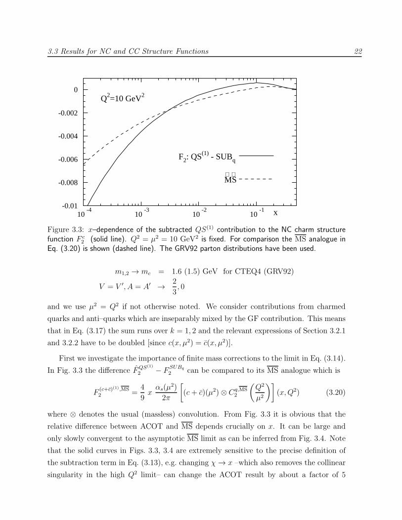
Figure 3.3: x–dependence of the subtracted QS(1) contribution to the NC charm structurefunction F c

2 (solid line). Q2 = µ2 = 10 GeV2 is fixed. For comparison the MS analogue inEq. (3.20) is shown (dashed line). The GRV92 parton distributions have been used.

m1,2 → mc = 1.6 (1.5) GeV for CTEQ4 (GRV92)

V = V ′, A = A′ → 2

3, 0

and we use µ2 = Q2 if not otherwise noted. We consider contributions from charmed

quarks and anti–quarks which are inseparably mixed by the GF contribution. This means

that in Eq. (3.17) the sum runs over k = 1, 2 and the relevant expressions of Section 3.2.1

and 3.2.2 have to be doubled [since c(x, µ2) = c(x, µ2)].

First we investigate the importance of finite mass corrections to the limit in Eq. (3.14).

In Fig. 3.3 the difference FQS(1)

2 − FSUBq

2 can be compared to its MS analogue which is

F(c+c)(1),MS2 =

4

9xαs(µ

2)

2π

[(c+ c)(µ2)⊗ Cq,MS

2

(Q2

µ2

)](x,Q2) (3.20)

where ⊗ denotes the usual (massless) convolution. From Fig. 3.3 it is obvious that the

relative difference between ACOT and MS depends crucially on x. It can be large and

only slowly convergent to the asymptotic MS limit as can be inferred from Fig. 3.4. Note

that the solid curves in Figs. 3.3, 3.4 are extremely sensitive to the precise definition of

the subtraction term in Eq. (3.13), e.g. changing χ → x –which also removes the collinear

singularity in the high Q2 limit– can change the ACOT result by about a factor of 5

3.3 Results for NC and CC Structure Functions 23

Q2 [GeV2]

x = 0.05

F2: QS(1) - SUBq

M

S

-0.1

0

0.1

0.2

0.3

0.4

0.5

x 10-3

10 102

103

Figure 3.4: The same as Fig. 3.3 but varying Q2(= µ2) for fixed x.

around Q2 ∼ 5 GeV2.3 This is an example of the ambiguities in defining a variable flavor

number scheme which have been formulated in a systematic manner in [22].

The relative difference between the subtracted QS(1) contribution calculated along

ACOT and the corresponding MS contribution in Eq. (3.20) appears, however, phe-

nomenologically irrelevant if one considers the significance of these contributions to the

total charm structure function in Fig. 3.5. The complete O(α1s) result (solid line) is shown

over a wide range of Q2 together with its individual contributions from Eq. (3.18). It can

be clearly seen that the full massive QS(1) contribution is almost completely cancelled by

the subtraction term SUBq (Indeed the curves for QS(1) and SUBq are hardly distinguish-

able on the scale of Fig. 3.5). The subtracted quark correction is numerically negligible

and turns out to be indeed suppressed compared to the gluon initiated contribution, which

is also shown in Fig. 3.5. Note, however, that the quark initiated corrections are not unim-

portant because they are intrinsically small. Rather the large massive contribution QS(1)

is perfectly cancelled by the subtraction term SUBq provided that µ2 = Q2 is chosen.

This is not necessarily the case for different choices of µ2 as we will now demonstrate.

In Fig. 3.6 we show the dependence of the complete structure function and its com-

ponents on the arbitrary factorization scale µ2. Apart from the canonical choice µ2 = Q2

3The subtracted gluon contribution GF changes by about a factor of 2 under the same replacement.

3.3 Results for NC and CC Structure Functions 24F 2c (x

,Q2 )

Q2 [GeV2]

x = 0.005

total O(αs1)

O(αs0): QS(0)

O(αs1): GF,QS(1) (unsubtr.)

SUBg,q

SUBg

QS(1)

GF

SUBq

-0.1

0

0.1

0.2

0.3

0.4

10 102

103

Figure 3.5: The complete O(α1s) neutral current structure function F c

2 and all individualcontributions over a wide range of Q2, calculated from the CTEQ4M distributions. Details ofthe distinct contributions are given in the text.

(which was used for all preceding figures) also different scales have been proposed [58, 59]

like the maximum transverse momentum of the outgoing heavy quark which is approx-

imately given by (pmaxT )2 ≃ (1/x − 1) Q2/4. For low values of x, where heavy quark

structure functions are most important, the scale (pmaxT )2 ≫ Q2. The effect of choosing

a µ2 which differs much from Q2 can be easiest understood for the massless coefficient

functions Cq,g,MSi which contain an unresummed ln(Q2/µ2). The latter is of course absent

for µ2 = Q2 but becomes numerically increasingly important, the more µ2 deviates from

Q2. This logarithmic contribution cannot be neglected since it is the unresummed part

of the collinear divergence which is necessary to define the scale dependence of the charm

density. This expectation is confirmed by Fig. 3.6. For larger values of µ2 the subtracted

QS(1) contribution is indeed still suppressed relative to the subtracted GF contribution.

Nevertheless, its contribution to the total structure function becomes numerically signifi-

cant and reaches the ∼ 20 % level around (pmaxT )2. Note that in this regime the involved

formulae of Section 3.2.2 may be safely approximated by the much simpler convolution

in Eq. (3.20) because they are completely dominated by the universal collinear logarithm

and the finite differences ACOT−MS from Figs. 3.3 and 3.4 become immaterial. In prac-

tice it is therefore always legitimate to approximate the ACOT results of Section 3.2.2 by

their MS analogues because both are either numerically insubstantial or logarithmically

3.3 Results for NC and CC Structure Functions 25F 2c (x

,Q2 )

µ2/Q2

∼ p Tmax

x = 0.005

Q2 = 25 GeV2

total O(αs1)

QS(0) + GF - SUBg

GF - SUBg

QS(1) - SUBq

-0.25

-0.2

-0.15

-0.1

-0.05

0

0.05

0.1

0.15

0.2

0.25

10-1

1 10 102

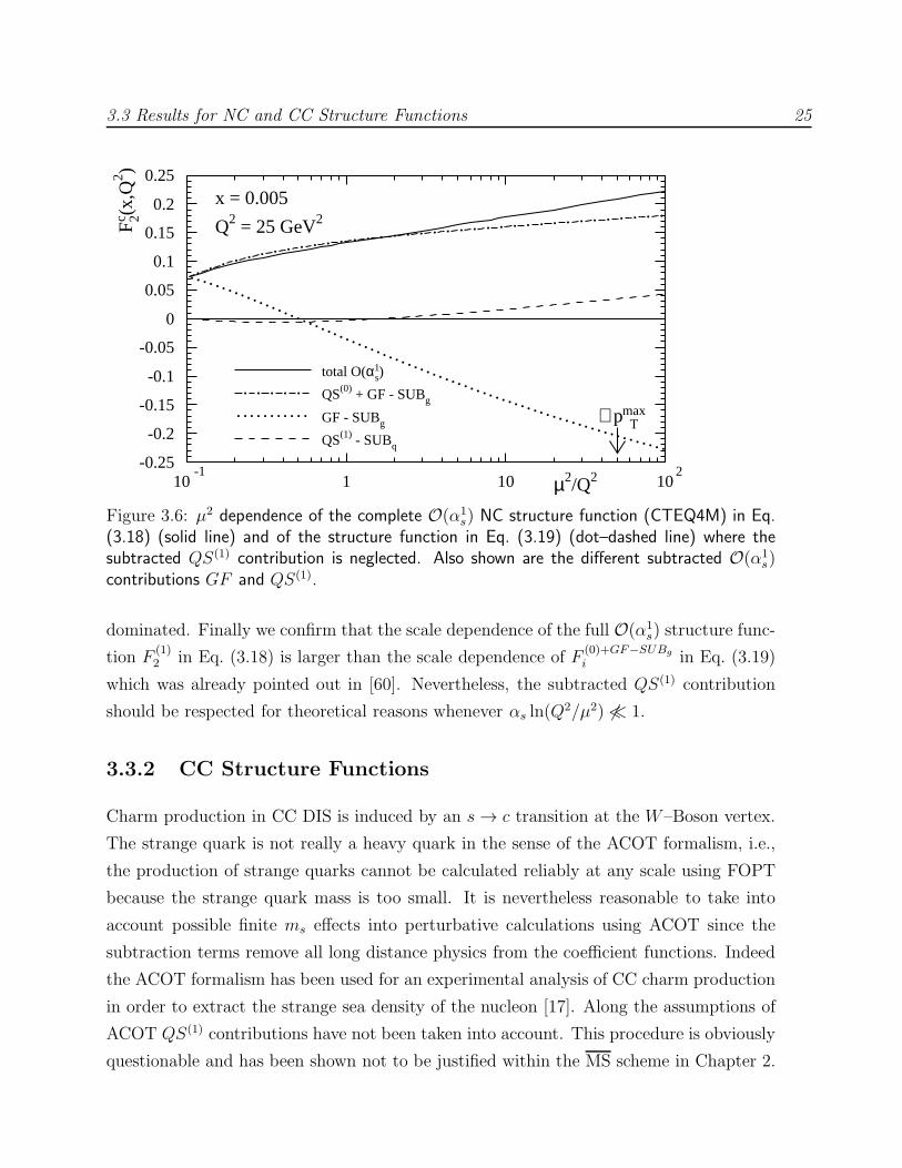
Figure 3.6: µ2 dependence of the complete O(α1s) NC structure function (CTEQ4M) in Eq.

(3.18) (solid line) and of the structure function in Eq. (3.19) (dot–dashed line) where thesubtracted QS(1) contribution is neglected. Also shown are the different subtracted O(α1

s)contributions GF and QS(1).

dominated. Finally we confirm that the scale dependence of the full O(α1s) structure func-

tion F(1)2 in Eq. (3.18) is larger than the scale dependence of F

(0)+GF−SUBg

i in Eq. (3.19)

which was already pointed out in [60]. Nevertheless, the subtracted QS(1) contribution

should be respected for theoretical reasons whenever αs ln(Q2/µ2) 6≪ 1.

3.3.2 CC Structure Functions

Charm production in CC DIS is induced by an s → c transition at the W–Boson vertex.

The strange quark is not really a heavy quark in the sense of the ACOT formalism, i.e.,

the production of strange quarks cannot be calculated reliably at any scale using FOPT

because the strange quark mass is too small. It is nevertheless reasonable to take into

account possible finite ms effects into perturbative calculations using ACOT since the

subtraction terms remove all long distance physics from the coefficient functions. Indeed

the ACOT formalism has been used for an experimental analysis of CC charm production

in order to extract the strange sea density of the nucleon [17]. Along the assumptions of

ACOT QS(1) contributions have not been taken into account. This procedure is obviously

questionable and has been shown not to be justified within the MS scheme in Chapter 2.

3.3 Results for NC and CC Structure Functions 26

With our results in Section 3.2.2 we can investigate the importance of quark initiated

O(α1s) corrections within the ACOT scheme for inclusive CC DIS. As already mentioned

above, results for the experimentally more important case of semi–inclusive (z–dependent)

DIS will be presented in Chapter 4 of this thesis. In the following we only introduce

subtraction terms for collinear divergencies correlated with the strange mass and treat

all logarithms of the charm mass along FOPT. We do so for two reasons, one theoretical

and one experimental: First, at present experimental scales of CC charm production

ln(Q2/m2c) terms can be safely treated along FOPT and no introduction of an a priori

unknown charm density is necessary. Second, the introduction of a subtraction term for

the mass singularity of the charm quark would simultaneously require the inclusion of the

c → s QS–transition at the W–vertex with no spectator–like c–quark as in GF . This

contribution must, however, be absent when experiments tag on charm in the final state.

CC DIS on massive charm quarks without final–state charm tagging has been studied in

[61].

The numerics of this section can be obtained by the formulae of Section 3.2 with the

following identifications:

Q1 → s , Q2 → c

m2 → mc = 1.5 GeV (GRV94)

V = V ′, A = A′ → 1, 1

and the strange mass m1 = ms will be varied in order to show its effect on the structure

function F c2 .

In Fig. 3.7 we show the structure function F c2 and its individual contributions for two

experimental values of x and Q2 [16] under variation of the factorization scale µ2. Like in

the NC case we show the complete O(α1s) result as well as F

(0)+GF−SUBg

2 where QS(1) has

been neglected. The thick curves in Fig. 3.7 (a) have been obtained with a regularizing

strange mass of 10 MeV. They are numerically indistinguishable from the ms = 0 MS

results along the lines of [49]. For the thin curves a larger strange mass of 500 MeV has

been assumed as an upper limit. Finite mass effects can therefore be inferred from the

difference between the thin and the thick curves. Obviously they are very small for all

contributions and can be safely neglected. For the higher Q2 value of Fig. 3.7 (b) they

would be completely invisible, so we only show the ms =10 MeV results (≡MS). Since the

finite mass corrections within the ACOT scheme turn out to be negligible as compared

3.3 Results for NC and CC Structure Functions 27

-0.2

-0.15

-0.1

-0.05

0

0.05

0.1

0.15

0.2

0.25

0.3

10-1

1 10 102

total O(αs1)

QS(0) + GF - SUBg

GF - SUBg

QS(1) - SUBq

x = 0.015Q2 = 2.4 GeV2

µ2/(Q2+mc2)(a)

F 2c (x,Q

2 )

∼ 2p Tmax

µ2/(Q2+mc2)(b)

F 2c (x,Q

2 )

x = 0.125

Q2 = 17.9 GeV2

∼ 2p Tmax

-0.02

0

0.02

0.04

0.06

0.08

0.1

10-1

1 10 102

Figure 3.7: The charm production contribution to the charged current structure functionF2 for a wide range of the factorization scale µ2 using GRV94. The curves are as for theneutral current case in Fig. 3.6. In Fig. 3.7 (a) the thicker curves have been obtained witha (purely regularizing) strange mass of 10 MeV which according to Eq. (3.14) (and to theanalogous limit for the subtracted GF term [20]) numerically reproduces MS. For the thinnercurves a strange mass of 500 MeV has been assumed. In Fig. 3.7 (b) all curves correspondto ms = 10 MeV (≡ MS).

3.4 Conclusions 28

to massless MS it is not surprising that we confirm the findings of Chapter 2 concerning

the importance of quark initiated corrections. They are –in the case of CC production of

charm– not suppressed with respect to gluon initiated corrections for all reasonable values

of the factorization scale. Only for small choices of µ2 ∼ Q2 +m2c can the quark initiated

correction be neglected. In this region of µ2 also gluon initiated corrections are moderate

and Born approximation holds within ∼ 10%. For reasons explained in Section 3.3.1 the

absolute value of both corrections –gluon and quark initiated– become very significant

when large factorization scales like pmaxT are chosen. This can be inferred by looking at

the region indicated by the arrow in Fig. 3.7 which marks the scale µ = 2pmaxT which was

used in [17]. Analyses which use ACOT with a high factorization scale and neglect quark

initiated corrections therefore undershoot the complete O(α1s) result by the difference

between the solid and the dot–dashed curve, which can be easily as large as ∼ 20 %. For

reasons explained in the introduction to this section we have used the radiative strange

sea of GRV94. When larger strange seas like CTEQ4 are used the inclusion of the quark

initiated contributions is even more important.

3.4 Conclusions

In this chapter we have calculated and analyzed DIS on massive quarks atO(α1s) within the

ACOT scheme for heavy quarks. For NC DIS this contribution differs significantly from its

massless MS analogue for µ2 = Q2. Both give, however, a very small contribution to the

total charm structure function such that the large relative difference is phenomenologically

immaterial. At higher values of the factorization scale µ2 ∼ (pmaxT )2 the contributions

become significant and their relative difference vanishes. TheQS(1) contribution of Section

3.2.2 can therefore be safely approximated by its much simpler MS analogue at any scale.

For CC DIS quark initiated corrections should always be taken into account on the same

level as gluon initiated corrections. Due to the smallness of the strange quark mass ACOT

gives results which are almost identical to MS.

Chapter 4

Charm Fragmentation in DeepInelastic Scattering

This chapter generalizes the theoretical considerations of Chapter 3 to the semi–inclusive

deep inelastic production of heavy flavored hadrons. We apply these results to the CC

and NC production of charm where we investigate the universality of charm fragmentation

functions and the charm production dynamics, respectively. The work in this chapter is

based on [4].

4.1 Introduction

In the preceeding chapter we have analyzed heavy quark initiated contributions to fully

inclusive deep inelastic (DI) structure functions. Towards lower values of the Bjorken

variable x, heavy (charm) quarks are produced in about 20% of the neutral current (NC)

[11–13] and charged current (CC) [43] deep inelastic events in lepton–nucleon collisions.

Therefore in this kinematical range, heavy quark events contribute an important compo-

nent to the fully inclusive DI structure functions of the nucleon. However, due to accep-

tance losses this component can usually not be measured directly by inclusively tagging on

charm events and more differential observables have to be considered like ED [16, 17, 45],

pT or η [11–13, 15] distributions, where ED, pT and η are the energy, transverse momen-

tum and pseudorapidity of the charmed hadron produced, i.e. mainly of a D(∗) meson. In

this chapter we consider ED spectra represented by the usual scaling variable z defined

below. Within DIS the charmed hadron energy spectrum is the distribution which is most

sensitive to the charm fragmentation process and may give complementary information

4.1 Introduction 30

to one hadron inclusive e+e− annihilation which is usually chosen to define fragmentation

functions (FFs) [29, 62]. A well understanding of charm fragmentation is essential for any

charm observable, e.g. the normalization of pT and η distributions in photoproduction is

substantially influenced by the hardness of the FF [63, 64]. The z distribution of charm

fragments is directly measured in CC neutrinoproduction [16, 17, 45] and may give insight

into details of the charm production dynamics in NC electroproduction. It has, e.g., been

shown in [11, 12] that the energy spectrum of D(∗)–mesons produced at the ep collider

HERA may be able to discriminate between intrinsic and extrinsic production of charm

quarks.

Intrinsic heavy quark densities may arise due to a nonperturbative component of the

nucleon wave function [55] or due to a perturbative resummation [20, 22–24] of large

quasi–collinear logs [ln(Q2/m2); Q and m being the virtuality of the mediated gauge

boson and the heavy quark mass, respectively] arising at any order in fixed order extrinsic

production (or fixed order perturbation theory: FOPT). Here we will only consider the

latter possibility for inducing an intrinsic charm density c(x,Q2) which is concentrated

at small x and we will ignore nonperturbative components which are expected to be

located at large x [55]. Technically the resummation of large perturbative logs proceeds

through calculating the boundary conditions for a transformation of the factorization

scheme [23, 47, 51], which is switched from nf to nf+1 active, massless flavors, canonically

at Q2 = m2. For fully inclusive DIS the Kinoshita–Lee–Nauenberg theorem confines all

quasi–collinear logs to the initial state such that they may be absorbed into c(x,Q2). For

semi–inclusive DIS (SI DIS) also final state collinearities arise which are resummed in

perturbative fragmentation functions Dci (z, Q

2) (parton i decaying into charm quark c)

along the lines of [51, 63]. The scale dependence of c(x,Q2) and Dci (z, Q

2) is governed by

massless renormalization group (RG) evolution.

Besides this zero mass variable flavor number scheme, where mass effects are only taken

care of by the boundary conditions for c(x,Q2) and Dci (z, Q

2), variable flavor number

schemes have been formulated [20, 22–24], which aim at resumming the quasi–collinear

logs as outlined above while also keeping power suppressed terms of O[(m2/Q2)k] in the

perturbative coefficient functions. Our reference scheme for this type of schemes will be

the one developed by Aivazis, Collins, Olness and Tung (ACOT) [19–21]. In the ACOT

scheme full dependence on the heavy quark mass is kept in graphs containing heavy

quark lines. This gives rise to the above mentioned quasi–collinear logs and to the power

4.2 Semi–Inclusive Heavy Quark Structure Functions 31

suppressed terms. While the latter are regarded as mass corrections to the massless,

dimensionally regularized, standard coefficient functions (e.g. in the MS scheme), the

former are removed numerically by subtraction terms, which are obtained from the small

mass limit of the massive coefficient functions.

The outline of this chapter will be the following: In Section 4.2 we will shortly overview

the relevant formulae for SI DIS for general masses and couplings including quark scat-

tering (QS) and boson gluon fusion (GF) contributions up to O(α1s). We will thereby

present our ACOT based calculation for the QS(1)1 component of SI structure functions.

In Section 4.3 we will analyze the charm fragmentation function in CC and NC DIS. In

Section 4.4 we draw our conclusions and some uncomfortably long formulae are relegated

to Appendix B.

4.2 Semi–Inclusive Heavy Quark Structure Func-

tions

This section presents the relevant formulae for one (heavy flavored) hadron inclusive DIS

structure functions. The contributions from scattering events on massive quarks are given

up to O(α1s) in Section 4.2.1 and GF contributions are briefly recalled in Section 4.2.2.

Section 4.2.3 presents all subtraction terms which render the structure functions infrared

safe and includes a discussion of these terms.

4.2.1 Scattering on Massive Quarks

We consider DIS of the virtual Boson B∗ with momentum q on the quark Q1 with mass

m1 and momentum p1 producing the quark Q2 with mass m2 and momentum p2. The

latter fragments into a heavy quark flavored hadron HQ2, e.g. a |Q2ql〉 meson, ql being any

light quark. Phenomenologically most prominent are of course charm quarks fragmenting

into D(∗)–mesons which are the lightest heavy flavored hadrons.

We will strictly take over the formulae and notations of our inclusive analysis in

Chapter 3 whenever possible and merely extend them for SI DIS considered here. In

particular we take over the definition of the structure functions Fi given in terms of the

usual experimental structure functions Fi in Eq. (3.8).

1Bracketed upper indices count powers of αs.

4.2 Semi–Inclusive Heavy Quark Structure Functions 32

Since we want to investigate the energy spectrum of charm fragments, we introduce

the Lorentz–invariant z ≡ pHQ2· pN/q · pN which reduces to the energy EHQ2

scaled to

its maximal value ν = q0 in the target rest frame. Therefore in contrast to Eq. (A.4) we

do not integrate the tensor ωµν over the full partonic phase space but keep it differential

in the corresponding partonic variable z′ ≡ p2 · p1/q · p1 or the mass corrected variable z

which is defined below. In order to obtain hadronic observables we have to extend the

Ansatz of Eq. (17) in [19] such that it includes a nonperturbative hadronization function

DQ2. In the limit of vanishing masses the massless parton model expressions have to be

recovered. Our Ansatz will be

W µν =

∫dξ

ξ

dζ

ζQ1(ξ, µ

2) DQ2(ζ, [µ2]) ωµν |{p+1 =ξP+;z=ζz} , (4.1)

where µ is the factorization scale, z = z′/z′LO with z′LO = Σ++/Σ+−and v+ ≡ (v0+v3)/

√2

for a general vector v. W µν is the usual hadronic tensor and ωµν is its partonic analogue.

Eq. (4.1) defines the fragmentation function DQ2 to be a multiplicative factor multiplying

inclusive structure functions at LO/Born accuracy, i.e.

FQS(0)

i=1,2,3(x, z, Q2) = FQS(0)

i=1,2,3(x,Q2) DQ2(z, [Q

2]) , (4.2)

where the FQS(0)

i=1,2,3(x,Q2) are defined and given in (3.8). The scale dependence of DQ2 is

bracketed here and in the following because it is optional; a more detailed discussion on

this point will be given at the end of Section 4.2.3. We do not construct our Ansatz in Eq.

(4.1) for the convolution of the fragmentation function along light front components for

the outgoing particles which would only be Lorentz–invariant for boosts along a specified

axis. Since the final state of DIS is spread over the entire solid angle it has no preferred

axis as defined for the initial state by the beam direction of collider experiments. Note

that Eq. (4.1) is in agreement with usual factorized expressions for massless initial state

quanta, as considered, e.g., in Chapter 2, since there m1 = 0 such that z′LO = 1.

Up to O(α1s) the hadronic structure functions for scattering on a heavy quark read

FQS(0+1)

i=1,2,3 (x, z, Q2, µ2) = Q1(χ, µ2) DQ2(z, [µ

2]) +αs(µ

2)

2π

∫ 1

χ

dξ′

ξ′

∫ 1

z

dz

z(4.3)

×[Q1

(χ

ξ′, µ2

)Hq

i (ξ′, z′, µ2) Θq

]DQ2

(zz, [µ2]

),

with [19]

χ =x

2Q2( Σ+−

+ ∆ ) . (4.4)

4.2 Semi–Inclusive Heavy Quark Structure Functions 33

As throughout this thesis we set the renormalization scale equal to the factorization scale

In Eq. (4.3). The kinematical boundaries of the phase space in Eq. (4.3) are introduced

by the theta function cut Θq. In the massless limit Θq → 1. The precise arguments of Θq

are set by the kinematical requirement

z′min < z′ < z′max , (4.5)

with

z′maxmin

=±∆[s, m2

1,−Q2](s−m22) + (Q2 +m2

1 + s)(s+m22)

2s(s−m21 +Q2)

,

where s = (p1 + q)2. Note that Eq. (4.5) also poses an implicit constraint on ξ′ via

z′min < z′max.

The Hqi for nonzero masses are obtained in exactly the same way as outlined for

fully inclusive structure functions in Appendix A if the partonic phase space is not fully

integrated over. They are given by

Hqi (ξ

′, z′) = CF

[(Si + Vi) δ(1− ξ′) δ(1− z)

+1− ξ′

(1− ξ′)+

z′LO8

s1 + Σ+−

∆′ N−1i fQ

i (s1, t1)], (4.6)

where the normalization factors Ni are given in Appendix A.3 and the Mandelstam vari-

ables read

s1(ξ′) ≡ (p1 + q)2 −m2

2

=1− ξ′

2ξ′[(∆− Σ+−

)ξ′ +∆+ Σ+−]

t1(ξ′, z′) ≡ (p1 − p3)

2 −m21

= [s1(ξ′) + Σ+−

](z′ − z′0) ,

where z′0 =s1 + Σ++

s1 + Σ+−

is the would–be pole of the t–channel propagator and we use ∆′ ≡

∆[s, m21,−Q2]. Si and Vi are the soft real and virtual contribution to Hq

i , respectively.

They can be found in Appendix A.3 whereas the fQi (s1, t1) are listed in Appendix B. In

the massless limit the Hqi reduce to the MS coefficient functions in [29, 30] up to some

divergent subtraction terms which we will specify in Section 4.2.3.

4.2 Semi–Inclusive Heavy Quark Structure Functions 34

4.2.2 Gluon Fusion Contributions at O(α1s)

We have already obtained the semi–inclusive coefficient functions for GF production of

massive quarks for general masses and couplings in Chapter 2. They are given by

FGF1,3 (x, z, Q2, µ2) =

∫ 1

ax

dx′

x′

∫ 1

z

dζ

ζg(x′, µ2) f1,3(

x

x′ , ζ, Q2) DQ2(

z

ζ, [µ2]) Θg

FGF2 (x, z, Q2, µ2) =

∫ 1

ax

dx′

x′

∫ 1

z

dζ

ζx′g(x′, µ2) f2(

x

x′ , ζ, Q2) DQ2(

z

ζ, [µ2]) Θg (4.7)

with the fi from Eq. (2.2) and ax = [1 + (m1 +m2)2/Q2]x. The Θg cut guarantees that

ζmin < ζ < ζmax where ζmin,max are given in Eq. (2.3). Similarly to Eq. (4.5) ζmin < ζmax

may also constrain the phase space available for the x′ integration.

4.2.3 Subtraction Terms

It requires three MS subtraction terms to render the double convolutions in Eqs. (4.3),

(4.7) infrared safe:

FSUBq

i (x, z, Q2, µ2) =αs(µ

2)

2πCF

∫ 1

χ

dξ′

ξ′

[1 + ξ′2

1− ξ′

(ln

µ2

m21

− 1− 2 ln(1− ξ′)

)]

+

× Q1

(χ

ξ′, µ2

)DQ2(z, [µ

2]) (4.8)

FSUBg

i (x, z, Q2, µ2) = DQ2(z, [µ2])

αs(µ2)

2πln

µ2

m21

∫ 1

χ

dξ′

ξ′P (0)qg (ξ′) g

(χ

ξ′, µ2

)(4.9)

FSUBD

i (x, z, Q2, µ2) =αs(µ

2)

2πCF

∫ 1

z

dz′

z′

[1 + z′2

1− z′

(ln

µ2

m22

− 1− 2 ln(1− z′)

)]

+

× DQ2

( zz′, µ2)

Q1

(χ, µ2

), (4.10)

where P(0)qg (ξ′) = 1/2 [ξ′2 + (1 − ξ′)2]. Note that SUBg in Eq. (4.9) differs slightly from

Eq. (2.6) in Chapter 2 because we are allowing for a nonzero initial state parton mass m1

here which we did not in Chapter 2.

The subtraction terms define the running of the initial state quark density (SUBq,

SUBg) and the final state fragmentation function (SUBD) in the massless limit. They

4.2 Semi–Inclusive Heavy Quark Structure Functions 35

remove collinear logarithms and scheme defining finite terms from the convolutions in

Eqs. (4.3), (4.7) and they are constructed such that the massless MS results of [29, 30] are

recovered in the limit

limm1,2→0

[FQS(0+1)+GF

i (x, z, Q2, µ2)−FSUBq+SUBg+SUBD

i (x, z, Q2, µ2)]= F (1),MS

i (x, z, Q2) ,

(4.11)

where SUBq and SUBD regularize FQS(0+1)

i whereas SUBg regularizes FGFi . Contrary

to the fully inclusive SUBg term in Eq. (3.17) there is no need to include an additional

∼ ln(µ2/m22) subtraction in Eq. (4.9) because the ζ−1 u–channel singularity of the massless

limit of GF (1) is located at ζ = 0 and is outside the integration volume of Eq. (4.7). If only

initial state subtractions, i.e. SUBq and SUBg, are considered and final state subtractions,

i.e. SUBD, are not performed one reproduces, in the limit m1 → 0 the results in [31, 50]

for producing a heavy quark from a light quark. Note that in this case the fragmentation

functionDQ2 should be taken scale–independent, say of the Peterson form [37]. In the limit

where also the final state quark mass m2 approaches zero and the final state subtraction

term SUBD is subtracted from the results in [31, 50]2 the massless quark results in [29, 30]

are obtained and a running ofDQ2 is induced via a RG resummation of final state collinear

logs as formulated for one hadron inclusive e+e− annihilation in [51, 63].

Apart from removing the long distance physics from the coefficient functions the sub-

traction terms set the boundary conditions for the intrinsic heavy quark density Q1 [47]

and the perturbative part of the heavy quark fragmentation function DQ2 [51]:

Q1(x,Q20) =

αs(Q20)

2πln

Q20

m21

∫ 1

x

dξ

ξP (0)qg (ξ) g

(x

ξ,Q2

0

)(4.12)

DQ2(z, Q20) =

αs(Q20)

2πCF

∫ 1

z

dz′

z′

[1 + z′2

1− z′

(ln

Q20

m22

− 1− 2 ln(1− z′)

)]

+

DQ2

( z

z′

)

(4.13)

where Q0, Q0 are the transition scales at which the factorization scheme is switched

from nf to nf + 1, nf + 2 active flavors, respectively (assuming here for simplicity that

m1 < m2; a generalization to m1 ≥ m2 is straightforward). For general Q0 also the gluon

density and αs undergo a scheme transformation. Canonically Q0 is set equal to the heavy

quark mass m1 which guarantees [47] up to two loops a continuous evolution of αs and

2See Equation (B.11) in [50].

4.2 Semi–Inclusive Heavy Quark Structure Functions 36

the light parton densities across Q0. All available heavy quark densities are generated

using Q0 = m1 and we will therefore follow this choice here although a variation of Q0

might substantially influence the heavy quark results even far above the threshold [18]

as was found in [65]. Note that at three loops a continuous evolution across Q0 can no

longer be achieved, neither for the parton distributions [23] nor for αs [66]. Analogously

to Q0 = m1 we use Q0 = m2 throughout. In Eq. (4.13) we have made the distinction

between the scale dependent FF DQ2(z, Q20) and the scale independent FF DQ2(z) explicit.

Following the terminology in [51, 63] the latter corresponds to the nonperturbative part

of the former and describes the hadronization process at the end of the parton shower

which is described perturbatively by the massless RG evolution. Alternatively, DQ2(z)

corresponds to a scale–independent FF within FOPT where no collinear resummations

are performed. These two points of view may induce a scheme dependence if DQ2(z) is

fitted to data. In principle, the massless evolution equations generate nonzero FFs also

for light partons to decay into heavy flavored hadrons. These light→heavy contributions

are important at LEP energies [63] but can be safely neglected at the scales considered

here3 and we will assume Di 6=Q2(z, µ2) = 0 throughout.

4.2.4 SI Structure Functions at O(α1s)

In the next section we will consider three types of O(α1s) VFNS structure functions. The

first two are constructed at full O(α1s)

FQS(0+1)+GFi − F

SUBq+SUBg+[SUBD]i , (4.14)

where the inclusion or omission of the bracketed SUBD term corresponds to a running

or scale–independent fragmentation function, respectively, as discussed in the previous

section. It is somewhat unclear whether QS(1) contributions (and the corresponding

subtractions) should be considered on the same perturbative level as GF (1), see the in-

troduction to Chapter 3 for a more detailed discussion on that point. In the original

formulation of the ACOT scheme [20] QS(1) contributions are neglected at the level we

are considering here and we therefore do also consider this option via the partial O(α1s)

structure function

FQS(0)+GFi − F

SUBg

i . (4.15)

3We could therefore, in principle, restrict the evolution of the charm FF to the nonsinglet sector.

4.3 The Charm Fragmentation Function in SI DIS 37

For obtaining the numerical results of the next section the general formulae of this section

have to be adjusted by choosing masses and couplings according to the relevant NC and

CC values as in Section 3.3.1 and 3.3.2. For the CC case where Q1 should be identified

with strange quarks the boundary condition in Eq. (4.12) is inadequate since m2s ∼ Λ2

QCD

is below the perturbative regime of QCD. We will have recourse to standard strange seas

from the literature [41, 42] instead.

4.3 The Charm Fragmentation Function in SI DIS

We will investigate the charm fragmentation function in CC and in NC SI DIS. In CC

DIS the charm production mechanism is undebated since charm is dominantly produced

by scattering on light strange quanta. Our reasoning will therefore be that Dc is directly

accessible in CC DIS at relatively low spacelike momentum transfer. An extracted Dc can

then be applied to NC DIS, where it might give insight into the details of the production

dynamics [11]. Also a test of the universality [67] of the charm FF measured in CC DIS

and e+e− annihilation [63] would be an important issue directly related to the factorization

theorems [68] of perturbative QCD (pQCD).

All εc parameters discussed below refer to a Peterson type [37] functional form given

in Eq. (2.8)

4.3.1 CC DIS

In CC DIS at fixed target energies one does not expect to gain much insight into the charm

production process since charm is dominantly produced in scattering events on strange

quarks4 in the nucleon, thereby permitting an experimental determination of the strange

quark content of the nucleon [16, 17, 45, 46]. On the other hand the well understood

production mechanism makes a direct determination of the charm fragmentation function

feasible by measuring the energy spectrum of final state charm fragments. This is obvious

in leading order accuracy where5

dσLO ∝ s(χ)Dc(z) (4.16)

4We assume a vanishing Cabibbo angle. Our results remain, however, unchanged if the CKM sup-pressed d → c background is included.

5We will suppress some obvious scale–dependences in the following formulae and in their discussion.

4.3 The Charm Fragmentation Function in SI DIS 38

is directly proportional to Dc. More precisely, it is not z but the closely related energy of

the c → µν decay muon which can be observed in iron detectors [16, 17, 45]. The smear-

ing effects of the decay complicates the determination of the precise shape of Dc but only

weakly influences an extraction of 〈z〉 [45] which is valuable information if physically mo-

tivated one–parametric Ansatze [37, 69] for Dc are assumed. At NLO the production cross

section is no longer of the simple factorized form of Eq. (4.16) and double convolutions

(symbol ⊗ below) of the form of Eqs. (4.3), (4.7) have to be considered. However, to a

reasonable approximation

dσNLO = ([s⊗ dσs + g ⊗ dσg]⊗Dc) (x, z, Q2)

≡ dσLO K(x, z, Q2)

∝ s(χ) Dc(z) K(x, z, Q2)

≃ s(χ) Dx,Q2[Dc](z) (4.17)

holds also at NLO accuracy within experimental errors and for the limited kinematical

range of present data on neutrinoproduction of charm. In Eq. (4.17) the approximate

multiplicative factor D absorbs the precise K–factor K(x, z, Q2) obtained from a full

NLO QCD calculation. D is not a simple universal fragmentation function but a nontrivial

process–dependent functional which is, however, mainly sensitive on Dc and shows little

sensitivity on the exact parton distributions considered. The occurrence of x,Q2 and z

in Eq. (4.17) as indices and as a functional argument, respectively, reflects the fact that

the dependence on x and Q2 is much weaker than is on z. Eq. (4.17) tells us that s(χ)

fixes the normalization of dσ once K is known. On the other hand K (or D) can be

computed from Dc with little sensitivity on s(χ), such that s(χ) and Dc(z) decouple in

the production dynamics and can be simultaneously extracted. This point can be clearly

inferred from Fig. 4.1 where it is shown that the wide spread of CC charm production

predictions which were obtained in [31] using GRV94 [41] and CTEQ4 [42] strange seas

can be brought into good agreement by a mere change of the normalization given by the

ratio sGRV (χ)/sCTEQ4(χ). The remaining difference is not within present experimental

accuracy which can be inferred from the shaded band representing a parametrization

[31] of CCFR data [16]. High statistics neutrino data therefore offer an ideal scenario

to measure Dc complementary to an extraction from LEP data on e+e− → DX [63,

70, 71]. This has been first noted in [67] where also a successful test of the universality

4.3 The Charm Fragmentation Function in SI DIS 39

-0.15

-0.1

-0.05

0

0.05

0.1

0.15

0.2

0.25

0 0.1 0.2 0.3 0.4 0.5 0.6 0.7 0.8 0.9 1

(a)z

χ s(

χ,z,

Q2 ) ef

f

x = 0.015

Q2 = 2.4 GeV2

NLO (εc =0.06) : GRV 94NLO

CTEQ 4

CTEQ4 * s(χ,Q2)GRV 94/s(χ,Q2)CTEQ4

(b)z

χ s(

χ,z,

Q2 ) ef

f x = 0.125

Q2 = 17.9 GeV2

-0.02

0

0.02

0.04

0.06

0.08

0.1

0 0.1 0.2 0.3 0.4 0.5 0.6 0.7 0.8 0.9 1

Figure 4.1: The charm production cross section obtained in [31] for two x,Q2 points in theCCFR [16] kinematical regime. Up to a constant of normalization which was convenientlychosen in Eq. (4) of [31] seff represents the triple–differential cross section d3σ/dxdydzwhere x and y are standard and z ≡ pD · pN/q · pN . Shown are the predictions usingGRV94 [41] (solid) and CTEQ4 [42] (dashed) partons and a curve (dot–dashed) where thenormalization of the CTEQ4 prediction is changed by multiplying with the ratio of the strangeseas sGRV (χ)/sCTEQ(χ). For all curves a scale–independent Peterson FF with εc = 0.06 hasbeen used.

of the charm FF has been performed. With new data [16, 17, 45]6 at hand and with a

sounder theoretical understanding of neutrinoproduction of charm it would be desirable

to update the analysis in [67]. Nowadays one can in principle examine the possibility

of a uniform renormalization group transformation from spacelike momenta near above

the charm mass (νN → DX) to timelike momenta at the Z0 peak (e+e− → DX). In

[63, 70, 71] charm fragmentation functions extracted from LEP data have been tested

against pT and η distributions measured in photoproduction at HERA. However, we

believe that a comparison to z differential neutrinoproduction data is worthwhile beyond,

6Data from NuTeV [72, 73] are to be expected in the near future; µ± events observed at NOMADawait further analysis [74].

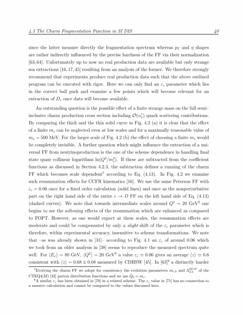
4.3 The Charm Fragmentation Function in SI DIS 40

since the latter measure directly the fragmentation spectrum whereas pT and η shapes

are rather indirectly influenced by the precise hardness of the FF via their normalization

[63, 64]. Unfortunately up to now no real production data are available but only strange

sea extractions [16, 17, 45] resulting from an analysis of the former. We therefore strongly

recommend that experiments produce real production data such that the above outlined

program can be executed with rigor. Here we can only find an εc parameter which lies

in the correct ball park and examine a few points which will become relevant for an

extraction of Dc once data will become available.

An outstanding question is the possible effect of a finite strange mass on the full semi–

inclusive charm production cross section including O(α1s) quark scattering contributions.

By comparing the thick and the thin solid curve in Fig. 4.2 (a) it is clear that the effect

of a finite ms can be neglected even at low scales and for a maximally reasonable value of

ms = 500 MeV. For the larger scale of Fig. 4.2 (b) the effect of choosing a finite ms would

be completely invisible. A further question which might influence the extraction of a uni-

versal FF from neutrinoproduction is the one of the scheme dependence in handling final

state quasi–collinear logarithms ln(Q2/m2c). If these are subtracted from the coefficient

functions as discussed in Section 4.2.3, the subtraction defines a running of the charm

FF which becomes scale dependent7 according to Eq. (4.13). In Fig. 4.2 we examine

such resummation effects for CCFR kinematics [16]. We use the same Peterson FF with

εc = 0.06 once for a fixed order calculation (solid lines) and once as the nonperturbative

part on the right hand side of the entire c → D FF on the left hand side of Eq. (4.13)

(dashed curves). We note that towards intermediate scales around Q2 ∼ 20 GeV2 one

begins to see the softening effects of the resummation which are enhanced as compared

to FOPT. However, as one would expect at these scales, the resummation effects are

moderate and could be compensated by only a slight shift of the εc parameter which is

therefore, within experimental accuracy, insensitive to scheme transformations. We note

that –as was already shown in [31]– according to Fig. 4.1 an εc of around 0.06 which

we took from an older analysis in [38] seems to reproduce the measured spectrum quite

well. For 〈Eν〉 = 80 GeV, 〈Q2〉 = 20 GeV2 a value εc ≃ 0.06 gives an average 〈z〉 ≃ 0.6

consistent with 〈z〉 = 0.68± 0.08 measured by CDHSW [45]. In [63]8 a distinctly harder

7Evolving the charm FF we adopt for consistency the evolution parameters mc,b and ΛQCD4,5 of the

CTEQ4(M) [42] parton distribution functions and we use Q0 = mc.8A similar εc has been obtained in [70] in a related scheme. The εc value in [71] has no connection to

a massive calculation and cannot be compared to the values discussed here.

4.3 The Charm Fragmentation Function in SI DIS 41

-0.15

-0.1

-0.05

0

0.05

0.1

0.15

0.2

0.25

0.1 0.2 0.3 0.4 0.5 0.6 0.7 0.8(a)

z

χ s(

χ,z,

Q2 ) ef

f x = 0.015

Q2 = 2.4 GeV2

mc = 1.6 GeV

NLO (εc =0.06) : fixed order:NLO

thick: ms = 0; thin: ms = 500 MeV

running FF

(b)z

χ s(

χ,z,

Q2 ) ef

f

x = 0.125

Q2 = 17.9 GeV2

CTEQ 4-0.04

-0.02

0

0.02

0.04

0.06

0.08

0.1

0.12

0.1 0.2 0.3 0.4 0.5 0.6 0.7 0.8

Figure 4.2: The same quantity as in Fig. 4.1. All predictions have been obtained for theCTEQ4 parton distributions. The solid curves result from a scale–independent Peterson FFwith εc = 0.06. In (a) the thin solid curve has been obtained using the formulae of Section4.2 and choosing a finite strange quark mass of ms = 500 MeV whereas the thicker curvecorresponds to the asymptotic ms → 0 limit (≡MS). In (b) these two options would becompletely indistinguishable and we only show the MS result. For the dot–dashed curves thefinal state quasi–collinear logarithm has been absorbed into a running of the charm FF. APeterson FF with εc = 0.06 has been used as the nonperturbative part of the input as givenin Eq. (4.13).

value of εc ≃ 0.02 was extracted from LEP data on e+e− → D∗X . If the latter fit is

evolved down to fixed target scales it is –even within the limited experimental accuracy–

incompatible with the CCFR neutrino data represented in Fig. 4.1. From Fig. 4.2 it is

clear that the difference cannot be attributed to a scheme dependence of the εc parameter

which is too small to explain the discrepancy. It would of course be interesting to know

how much the above mentioned smearing effect of the c → µν decay might dilute the dis-

crepancy. In any case, charm fragmentation at LEP has been measured by tagging on D∗s

whereas neutrinoproduction experiments observe mainly Ds through their semileptonic

decay–channel (dimuon events). ARGUS [75] and CLEO [76] data at√s ≃ 10GeV indeed

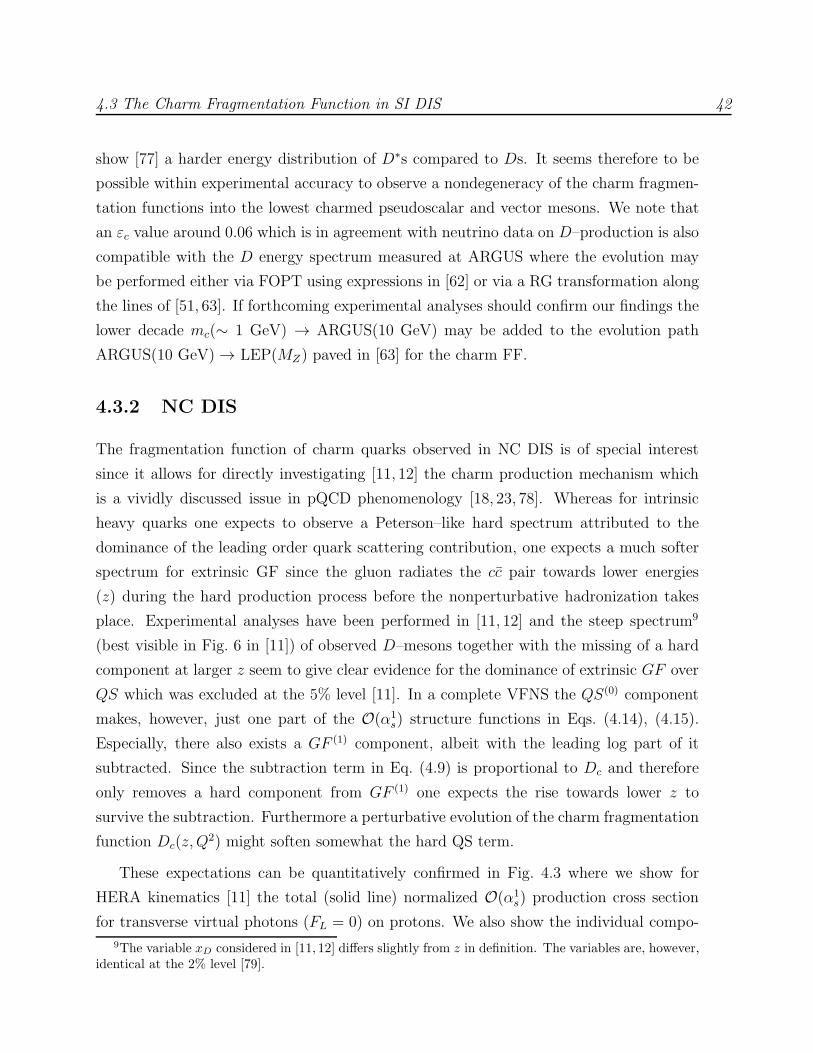
4.3 The Charm Fragmentation Function in SI DIS 42

show [77] a harder energy distribution of D∗s compared to Ds. It seems therefore to be

possible within experimental accuracy to observe a nondegeneracy of the charm fragmen-

tation functions into the lowest charmed pseudoscalar and vector mesons. We note that

an εc value around 0.06 which is in agreement with neutrino data on D–production is also

compatible with the D energy spectrum measured at ARGUS where the evolution may

be performed either via FOPT using expressions in [62] or via a RG transformation along

the lines of [51, 63]. If forthcoming experimental analyses should confirm our findings the

lower decade mc(∼ 1 GeV) → ARGUS(10 GeV) may be added to the evolution path

ARGUS(10 GeV) → LEP(MZ) paved in [63] for the charm FF.

4.3.2 NC DIS

The fragmentation function of charm quarks observed in NC DIS is of special interest

since it allows for directly investigating [11, 12] the charm production mechanism which

is a vividly discussed issue in pQCD phenomenology [18, 23, 78]. Whereas for intrinsic

heavy quarks one expects to observe a Peterson–like hard spectrum attributed to the

dominance of the leading order quark scattering contribution, one expects a much softer

spectrum for extrinsic GF since the gluon radiates the cc pair towards lower energies

(z) during the hard production process before the nonperturbative hadronization takes

place. Experimental analyses have been performed in [11, 12] and the steep spectrum9

(best visible in Fig. 6 in [11]) of observed D–mesons together with the missing of a hard

component at larger z seem to give clear evidence for the dominance of extrinsic GF over

QS which was excluded at the 5% level [11]. In a complete VFNS the QS(0) component

makes, however, just one part of the O(α1s) structure functions in Eqs. (4.14), (4.15).

Especially, there also exists a GF (1) component, albeit with the leading log part of it

subtracted. Since the subtraction term in Eq. (4.9) is proportional to Dc and therefore

only removes a hard component from GF (1) one expects the rise towards lower z to

survive the subtraction. Furthermore a perturbative evolution of the charm fragmentation

function Dc(z, Q2) might soften somewhat the hard QS term.

These expectations can be quantitatively confirmed in Fig. 4.3 where we show for

HERA kinematics [11] the total (solid line) normalized O(α1s) production cross section

for transverse virtual photons (FL = 0) on protons. We also show the individual compo-

9The variable xD considered in [11, 12] differs slightly from z in definition. The variables are, however,identical at the 2% level [79].

4.3 The Charm Fragmentation Function in SI DIS 43σ-1

dσ/

dz

z

total O(αs1)

Born (γ* c → c)(γ* c → c g)(γ* g → c c

– )

-1

-0.5

0

0.5

1

1.5

2

2.5

3

3.5

0 0.1 0.2 0.3 0.4 0.5 0.6 0.7 0.8 0.9 1

Figure 4.3: The normalized charm production cross section dσ/dz (z ≡ pD · pN/q · pN) forHERA kinematics (

√s = 314 GeV). For a comparison with H1 data [11] the cross section

has been integrated over 10 GeV2 < Q2 < 100 GeV2 and 0.01 < y < 0.7. Following theexperimental analysis [11] only contributions from transverse photons (FL = 0) are considered.Shown is the total O(α1

s) result (solid line) and the individual contributions. Details to thecalculation of the total result and the individual contributions are given in the text. The charmmass has been kept finite at the CTEQ4 value of mc = 1.6 GeV everywhere except for thethin dotted curve where the mc → 0 limit has been taken.

nents contributing to it: The processes γ∗g → cc (dot–dashed) and γ∗c → cg (dotted; incl.

virtual corrections) correspond to the GF (1) − SUBg and QS(1) − SUBq − SUBD terms,

respectively, subtracted at µ = Q. They are not physically observable and only sensible

if they are added to the QS(0) Born term (dashed) as in Eqs. (4.14), (4.15). We have per-

turbatively resummed all logarithms of the charm mass via massless evolution equations

starting at the charm mass [Q0 = Q0 = mc] and using the standard boundary conditions

in Eqs. (4.12), (4.13) for εc = 0.06. Finite charm mass effects on the subtracted QS(1)

contribution can be inferred by comparing the thick and the thin dotted curves, where the

mc → 0 limit has been taken for the latter. As has been theoretically anticipated in [21]

the charm mass can be safely set to zero in QS(1) and the involved convolutions in Eq.

(4.1) may be replaced by the massless expressions in [29, 30] which simplifies the numerics

essentially and which we will therefore do for the µ = 2mc curve in Fig. 4.4 below. As

also stressed in [21] it is, however, essential to keep the charm mass finite in the GF (1)

contribution since mc tempers the strength of the z′−1 u–channel propagator singularity.

4.3 The Charm Fragmentation Function in SI DIS 44σ-1

dσ/

dz

z

GF(1) (fixed order)

VFNS (ACOT):

total O(αs1)

QS(0) + GF - SUBg

µ=2mc

µ=Q

0

0.5

1

1.5

2

2.5

3

3.5

0 0.1 0.2 0.3 0.4 0.5 0.6 0.7 0.8 0.9 1

Figure 4.4: A Comparison of the total O(α1s) result (solid lines) to H1 data [11] onD

0 (circles)and D+∗

(triangles; both including charge conjugation) production. Shown are results for twochoices of the factorization/renormalization scale µ. Also shown is the outcome of a fixedorder O(α1

s) GF calculation for comparison (dashed line). The dot–dashed line follows thesuggestion in [20] and neglects quark initiated contributions at O(α1

s), i.e. the differencebetween the solid (µ = Q) and the dot–dashed line is given by the (thick) dotted line in Fig.4.3. For the dot–dashed curve as well as for the fixed order calculation (dashed) only µ = Qis shown since the scale dependence is completely insignificant.

Obviously the O(α1s) result of an ACOT based calculation deviates essentially from the

naive Born term expectation and it seems by no means legitimate to treat GF (1) as a

higher order correction here. Contrary to the corresponding inclusive results in Chapter

3 and to the expectations in [20] also the subtracted QS(1) term is numerically significant

in the semi–inclusive case considered here. In the light of the huge O(α1s) corrections

it seems, however, undecidable as to whether include or omit QS(1) at O(α1s) without

knowing O(α2s) corrections within ACOT.

In Fig. 4.4 the resummed result (VFNS: solid lines) can be compared to unsubtracted

O(α1s)

10 GF (1) (fixed order, dashed line). We show the total O(α1s) VFNS result for

the choices µ = Q, 2mc. The modest scale dependence arises exclusively through the

QS(1) term. For any of the other curves a variation of µ is completely insignificant

and we therefore only show µ = Q. A full VFNS calculation (solid lines) seems hardly

10An O(α2s) NLO calculation [80] within FOPT gives very similar results [79].

4.4 Conclusions 45

distinguishable from fixed order perturbation theory (dashed line) within experimental

accuracy. The two approaches are even closer if one follows the suggestion in [20] and

does not include (dot–dashed line) the subtracted QS(1) term at the level of QS(0) +

GF (1). The data points in the figure correspond to H1 measurements [11] of D0 (circles)

and D∗+ (triangles; both including charge conjugation) spectra. The measurement is

restricted to ηD < 1.5. Extrapolating to the full phase space gives rise to large acceptance

corrections which are, however, quite uniform [79] over the kinematical range considered

and therefore have a minor effect on the normalized spectrum. Since FOPT and ACOT

based calculations are very close it seems improbable that an experimental discrimination

between the two approaches will be possible. The Born term in Fig. 4.3 is far from being

the dominant contribution and an intrinsic c(x,Q2) stemming from the resummation

of perturbative logs can therefore not be excluded. The tendency of the data appears

somewhat softer than any of the calculations and the tendency seems to be confirmed by

preliminary data in a lower z bin [81]. The resummed calculation appears to be too hard

at larger z around 0.6 if the QS(1) component is included. As already mentioned, at the

present stage of the calculations it cannot be decided whether this hints at an intrinsic

problem within VFNS calculations or whether this may be cured by O(α2s) corrections.

4.4 Conclusions

In this chapter we have performed an ACOT [20] based analysis of heavy quark fragmen-

tation in DIS including a calculation of semi–inclusive scattering on massive quarks at

O(α1s) for general masses and couplings. As in the inclusive case of Chapter 3, effects

from finite initial state quark masses can be neglected for practical applications to charm

production in CC and NC DIS. The involved convolutions in Section 4.2.1 can therefore

safely be replaced by their analogues in [29, 30] and in Appendix B of [50]. Neutrinopro-

duction is an ideal environment to extract the charm FF within DIS and a Peterson [37]

type FF with εc ≃ 0.06 seems to lie in the correct ball park, where the sensitivity on

the choice of scheme is small and finite ms effects are irrelevant. The εc value above is

compatible with e+e− data if a nondegeneracy of charm quarks fragmenting into D and

D∗ mesons is allowed for. For NC DIS it seems unlikely that a discrimination between

fixed order and resummed calculations will be possible at HERA. Both approaches give

similar results which show a spectrum that is somewhat harder than the tendency of the

4.4 Conclusions 46

data [11, 12, 81]. The resummed calculation is made worse if the O(α1s) quark scattering

contribution is included at the perturbative level considered here.

Chapter 5

Summary

In the first part of this thesis we have studied deep inelastic production of heavy quarks

in neutral current and charged current processes. For this purpose we have calculated the

relevant partonic subprocesses to order O(α1s) (BGF, QS) for general masses and couplings

taking into account massive initial state quark–partons as needed in the variable flavor

number scheme of ACOT [20]. Our calculation of the vertex correction with general

masses and couplings is, to our best knowledge, new.

The integrated partonic results could be used to formulate and investigate heavy quark

contributions to inclusive deep inelastic structure functions within the ACOT variable

flavor number scheme. By the calculation of the before missing radiative corrections to

scattering amplitudes on massive quark partons (including virtual corrections) the ACOT

scheme could be completed to full order O(α1s). Furthermore, we utilized the unintegrated

partonic structure functions to extend the original ACOT scheme [20] from its inclusive

formulation to (z–differential) one–hadron–inclusive leptoproduction.

With help of these results we demonstrated in the charged current sector that the

effects of a finite strange mass are small and rapidly converge towards MS in the limit

ms → 0. Furthermore, it turned out that the effects of finite initial state masses can

be neglected in all cases, such that the (massive) QS(1) contribution of Section 3.2.2 can

safely be approximated by its much simpler MS analogue at any scale. Nevertheless, it

should be stressed that radiative corrections to quark initiated processes are in general

not negligible and should be included in complete NLO analyses employing heavy quark

parton densities.

Finally, we have performed an ACOT based analysis of heavy quark fragmentation in

48

DIS led by the observation that semi–inclusive CC DIS is well suited to extract the charm

fragmentation function. We reassured that theoretical uncertainties due to scheme choices

and finite ms effects are irrelevant and found out that a Peterson type fragmentation

function with εc ≈ 0.06 seems to lie in the correct ball park. The εc value above is

compatible with e+e− data if a nondegeneracy of charm quarks fragmenting into D and

D∗ mesons is allowed for. In the case of semi–inclusive NC DIS it seems unlikely that a

discrimination between fixed order and resummed calculations will be possible at HERA.

Both approaches gave similar results exhibiting a spectrum that is somewhat harder than

the tendency of the data [11, 12, 81]. The resummed calculation is made worse if the

O(α1s) quark scattering contribution is included at the perturbative level considered here.

Part II

The Structure of Real and VirtualPhotons

Chapter 6

Introduction and Survey

Photon physics is an active field of research as is documented by and in a large number of

reviews [82–91]. Particularly in the past few years there has been much progress due to

the wealth of experimental results from the e+e− collider LEP and the ep collider HERA

[90, 91]. Among the reactions initiated by high energy photons such processes providing

a hard scale are of particular interest since they can be described (at least partly) by

means of perturbative QCD. More precisely, in this thesis we are interested in processes

which can be described within the well known framework of the parton model and in

this case the ’hadronic nature of the photon’ is quantitatively described by the partonic

structure of the photon. The classical way of measuring the photonic parton content is

deep inelastic electron–photon scattering (DISeγ) which is the main source of information.

The DISeγ data on the photon structure function F γ2 (x,Q

2) are mainly sensitive to the

up–quark density uγ(x,Q2) as can be seen from the parton model expression for F γ2 (in

LO), F γ2 ∝ 4uγ + dγ + sγ, whereas the gluon distribution gγ(x,Q2) is only indirectly

constrained at small values of x due to the evolution. Complementary information has

become available in the last years due to ’resolved photon processes’ (e.g. production of

(di–)jets or hadrons with large pT (ET ), heavy quark production, isolated prompt photon

production) in γp and γγ collisions at HERA and LEP, respectively, which are mainly

sensitive to the gluon distribution in the photon. However, the experimental constraints

on the gluon density are still weak, especially at x < 0.1, and one has to resort to model

assumptions about the parton distributions of the photon.

It is the virtue of the phenomenologically successful radiative parton model (GRV

model) [26, 41, 57, 92, 93] to predict the small–x behavior of parton distributions by pure

51

DGLAP–evolution of valence–like input distributions at a low input scale µ2 ≃ 0.3 GeV2.

Recently, the parton distributions of the proton have been revised [26] due to precision

measurements of the proton structure function F p2 at HERA leading to slightly changed

parameters (low input scale, αs) and a less steep small–x increase compared to the previous

GRV94 [41]. In order to test quantitatively (within the GRV approach) if protons, pions

and photons show a similar small–x (i.e. high energy) behavior it is necessary to update

also the parton distributions of pions and photons.

At present e+e− and ep collider experiments the photon beams consist of

bremsstrahlung radiated off the incident lepton beam resulting in a continuous spec-

trum of target photons γ(P 2) where P 2 is the photon’s virtuality. The bremsstrahlung

spectrum is proportional to 1/P 2 such that the bulk of target photons is produced at

P 2 ≃ P 2min ≃ 0. The parton content of such (quasi–)real photons is well established both

experimentally and theoretically and it is quite natural to expect the parton distributions

to decrease smoothly with increasing P 2 and not to vanish immediately. In this sense the

real photon γ ≡ γ(P 2 ≃ 0) is just a ’primus inter pares’ and unified approaches to the

parton content of virtual photons γ(P 2) which comprise the real photon case in the limit

P 2 → 0 are highly desirable. This is also reflected by the fact that measurements of the

real photon structure function F γ2 in single–tag events integrate over the bremsstrahlung

spectrum from P 2min up to a P 2

max which depends on the experimental details. For instance,

at LEP1(LEP2) P 2max is as large as P 2

max ≃ 1.5 GeV2(4.5 GeV2), cf. Section 2.2 in [90].

Allthough the bulk of photons is produced at P 2 ≃ P 2min the amount of ignorance of the

P 2–dependence, mainly in the range P 2 . Λ2, feeds back on the determination of the

structure function F γ2 (parton distributions) of (quasi–)real photons.

It is the central goal of the second part of this thesis to perform LO and NLO

analyses of the parton content of pions and real and virtual photons within the latest

fine–tuned/improved setting of the GRV model [26].

The outline of Part II will be as follows:

• In Chapter 7 we provide the basic kinematical background for studying the structure

of real and virtual photons in two–photon scattering events. Structure functions

for virtual photons are defined in a general (model independent) way which will be

studied in the following chapters either in fixed order perturbation theory (Chapters

8, 12) or within the framework of the QCD–improved parton model (Chapters 9,

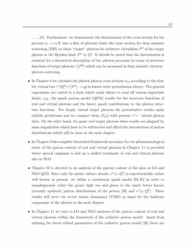
52

. . . , 12). Furthermore, we demonstrate the factorization of the cross section for the

process ee → eeX into a flux of photons times the cross section for deep inelastic

scattering (DIS) on these “target” photons for arbitrary virtualities P 2 of the target

photon in the Bjorken limit P 2 ≪ Q2. It should be noted that the factorization is

essential for a theoretical description of two–photon processes in terms of structure

functions of target photons γ(P 2) which can be measured in deep inelastic electron–

photon scattering.

• In Chapter 8 we calculate the photon photon cross sections σab according to the dou-

bly virtual box γ⋆(Q2)γ⋆(P 2) → qq in lowest order perturbation theory. The general

expressions are casted in a form which easily allows to read off various important

limits, e.g., the quark–parton model (QPM) results for the structure functions of

real and virtual photons and the heavy quark contributions to the photon struc-

ture functions. For deeply virtual target photons the perturbative results make

reliable predictions and we compare them (Feff) with present e+e− virtual photon

data. On the other hand, for quasi–real target photons these results are plagued by

mass singularities which have to be subtracted and afford the introduction of parton

distributions which will be done in the next chapter.

• In Chapter 9 the complete theoretical framework necessary for our phenomenological

study of the parton content of real and virtual photons in Chapter 11 is provided

where special emphasis is laid on a unified treatment of real and virtual photons

also in NLO.

• Chapter 10 is devoted to an analysis of the parton content of the pion in LO and

NLO QCD. Since only the pionic valence density vπ(x,Q2) is experimentally rather

well known at present, we utilize a constituent quark model [94, 95] in order to

unambiguously relate the pionic light sea and gluon to the much better known

(recently updated) parton distributions of the proton [26] and vπ(x,Q2). These

results will serve via vector meson dominance (VMD) as input for the hadronic

component of the photon in the next chapter.

• In Chapter 11 we turn to LO and NLO analyses of the parton content of real and

virtual photons within the framework of the radiative parton model. Apart from

utilizing the latest refined parameters of the radiative parton model [26] there are

53

some novelties as compared to the original GRVγ approach [96]. At first, the bound-

ary conditions for the real photon are based on a coherent superposition of vector

mesons which maximally enhances the up–quark contribution to the photon struc-

ture function F γ2 (x,Q

2) as is favored by the experimental data. As a result no extra

normalization factor for the photonic boundary conditions is needed. Furthermore,

in order to remove model ambiguities of the hadronic light quark sea and gluon

input distributions of the photon (being related to the ones of the pion via VMD),

inherent to the older GRVγ [96] and SaS [97] parametrizations, we employ, as al-

ready mentioned, predictions for the pionic light quark sea and gluon which follow

from constituent quark model constraints. The resulting predictions for the real

photon structure functions F γ2 (x,Q

2) will be compared with all presently (January

1999) available relevant data. Most recently the OPAL collaboration [98] at the

CERN–LEP collider has extended the measurements of the photon structure func-

tion F γ2 (x,Q

2) into the small–x region down to x ≃ 10−3, probing lower values of x

than ever before and we include a comparison with these data as well. Finally, we

construct LO and NLO boundary conditions for the virtual photon which allow for

a smooth transition to the real photon case and perform a careful study of the re-

sulting predictions for the partonic content and the structure function Fγ(P 2)2 (x,Q2)

of virtual photons.

• In Chapter 12 we test our model for the parton content of virtual photons in more

detail and compare these QCD–resummed results with the fixed order box expres-

sions of Chapter 8. It is demonstrated that present e+e− and DIS ep data on the

structure of the virtual photon can be understood entirely in terms of the standard

‘naive’ quark–parton model box approach. Thus the QCD–resummed (renormal-

ization group (RG) improved) parton distributions of virtual photons, in particular

their gluonic component, have not yet been observed. The appropriate kinematical

regions for their future observation are pointed out as well as suitable measurements

which may demonstrate their relevance.

• Finally, in Chapter 13 we summarize our main results and discuss open questions.

• Various limits of the doubly virtual box calculation and parametrizations of our

pionic and photonic parton distributions have been relegated to the Appendices C

and D, respectively.

Chapter 7

Photon–Photon Scattering

In this chapter we provide the basic kinematical background for studying the structure of

real and virtual photons in two–photon scattering events.

In Section 7.1 we give a short introduction into so–called two–photon processes, in-

troduce the usual kinematical variables to describe them and derive the cross section for

such events. The notation follows mainly the report of Budnev et al. [82]. Here we only

present a selection of the topic needed throughout the thesis. Additional information can

be found in [82] and, e.g., in the more recent reviews [85, 90].

Next, in Section 7.2 we define structure functions for virtual photons and relate them

to the photon–photon scattering cross sections. These structure functions will be studied

in the following chapters either in fixed order perturbation theory (Chapters 8, 12) or

within the framework of the QCD–improved parton model (Chapters 9, . . . , 12).

Finally, in Section 7.3 we demonstrate the factorization of the cross section for the

process ee → eeX into a flux of photons and the cross section for deep inelastic scattering

(DIS) on these “target” photons. While the factorization is well known for (quasi–)real

target photons with virtuality P 2 ≈ 0 we deal with the general P 2 6= 0 case in the Bjorken

limit. It should be noted that the factorization is essential for a theoretical description of

two–photon processes in terms of structure functions of the (real or virtual) photon.

7.1 Kinematics 55

7.1 Kinematics

The kinematics of particle production via photon–photon scattering in e+e− collisions

e−(p1)e+(p2) → e−(p′1)e

+(p′2)γ⋆(q)γ⋆(p) → e−(p′1)e

+(p′2)X(pX) (7.1)

is depicted in Fig. 7.1. The momenta of the incoming and outgoing leptons are denoted

p ↑

q ↓}X

p1

p2

p′1

p′2

−q2 = Q2 ≡ Q21

W 2 = (q + p)2

−p2 = P 2 ≡ Q22

Figure 7.1: Two–photon particle production. The solid lines are the incoming and outgoingleptons and the wavy lines are virtual photons which produce a final state X consisting ofhadrons (or leptons).

by pi ≡ (Ei, ~pi) and p′i ≡ (E ′i, ~pi

′) (i = 1, 2) respectively and the momenta of the photons

are given by

q ≡ p1 − p′1 , Q2= −q2 ≡ Q21 ,

p ≡ p2 − p′2 , P 2= −p2 ≡ Q22 .

(7.2)

In general both photons have spacelike momenta and P 2 refers to the photon with smaller

virtuality (P 2 ≤ Q2). X denotes the final state produced in the γ⋆(q) + γ⋆(p) → X

subprocess. For later use, we define the following variables:

ν = p · q , x =Q2

2ν, δ =

P 2

2ν, y1 =

p · qp · p1

, y2 =p · qq · p2

,

W 2 ≡ (p+ q)2 = 2ν(1− x− δ) = Q21− x

x− P 2 . (7.3)

7.1 Kinematics 56

Lµµ′(1)

Lνν′(2)

Wµ′ν′µν

q, µ

p, ν

q, µ′

p, ν ′

p1

p2

p′1

p′2

p1

p2

Figure 7.2: Squared matrix element of the process (7.1). Integration over the phase space ofthe system X is implied as indicated by the vertical cut.

The cross section for the process (7.1) is given by

dσ =1

Fee|M |2dQ(n+2) (7.4)

with the invariant matrix element M , the Møller flux factor of the two incoming leptons

Fee = 4√(p1 · p2)2 −m2

em2e , (7.5)

and the Lorentz–invariant (n + 2)–particle phase space

dQ(n+2)(p1 + p2; p′1, p

′2, k1, . . . , kn) =

d3p′1(2π)32E ′

1

d3p′2(2π)32E ′

2

dQ(n)(q + p; k1, . . . , kn)

=d3p′1

(2π)32E ′1

d3p′2(2π)32E ′

2

(2π)4δ(4) (q + p− pX) dΓ .

(7.6)

Here pX =∑

i ki, i ∈ X is the total momentum and dΓ =∏

id3ki

2k0i (2π)3 , i ∈ X the phase

space volume of the produced system X.

The cross section can be expressed in terms of the amplitudes Mµν of the γ⋆(q) +

γ⋆(p) → X subprocess as follows (see Fig. 7.2):

dσ =d3p′1d

3p′22E ′

12E′2(2π)

6

(4πα)2

Q4P 4

1

FeeLµµ′

(1) Lνν′

(2)Wµ′ν′,µν (7.7)

7.1 Kinematics 57

with

W µ′ν′,µν =1

2

∫M⋆µ′ν′Mµν(2π)4δ(4)(q + p− pX)dΓ . (7.8)

For unpolarized leptons the (leptonic) tensors L(1) and L(2) (see Fig. 7.2) are given by

Lαβ(i) =

1

2Tr[(p/i +me)γ

α(p/′i +me)γβ] . (7.9)

The factor 1/2 is due to a spin average over the incoming leptons. In addition, we

introduce the dimensionless quantities [82]

ραβi =1

Q2i

Lαβ(i) = −

(gαβ − qαi q

βi

q2i

)− (2pi − qi)

α(2pi − qi)β

q2i(7.10)

which have the interpretation of (unnormalized) density matrices for the corresponding

virtual photons.

7.1.1 The Hadronic Tensor W µ′ν′,µν

According to the optical theorem W µ′ν′,µν is the absorptive part of the virtual γγ forward

amplitude shown in Fig. 7.3.

q, µ,m

p, ν, n

q, µ′, m′

p, ν ′, n′

Figure 7.3: The photon–photon forward scattering amplitude T µ′ν′,µν ; m, n, m′, and n′ arehelicity indices. The tensor W µ′ν′,µν defined in (7.8) is the absorptive part of the γγ forwardamplitude: W µ′ν′,µν = 1

πImT µ′ν′,µν .

Taking into account P– and T–invariance (symmetry µ′ν ′ ↔ µν) and gauge invariance,

i.e.

qµWµ′ν′,µν = qµ′W µ′ν′,µν = pνW

µ′ν′,µν = pν′Wµ′ν′,µν = 0 ,

7.1 Kinematics 58

the Lorentz–tensor W µ′ν′,µν can be expanded in terms of a basis of 8 independent tensors

constructed from the vectors q, p and the metric tensor g. The choice of the tensor basis

in which the expansion is carried out is clearly arbitrary and different forms are discussed

in the literature [82, 99, 100]. In the following we will stick to the expansion given in [82]:

W µ′ν′,µν =Rµ′µRν′νWTT +Rµ′µQν2Q

ν′

2 WTL +Qµ′

1 Qµ1R

ν′νWLT +Qµ′

1 Qµ1Q

ν′

2 Qν2WLL

+1

2(Rµ′ν′Rµν +Rµ′νRν′µ −Rµ′µRν′ν)W τ

TT

− (RµνQµ′

1 Qν′

2 +Rν′µQµ′

1 Qν2 +Rµ′ν′Qµ

1Qν2 +Rµ′νQν′

2 Qµ1 )W

τTL

+ (Rµ′ν′Rµν −Rν′µRµ′ν)W aTT

− (RµνQµ′

1 Qν′

2 − Rν′µQµ′

1 Qν2 + Rµ′ν′Qµ

1Qν2 − Rµ′νQν′

2 Qµ1 )W

aTL .

(7.11)

The tensor structures used in (7.11) are connected to the photon polarization vectors, see

App. B and C in [82]:

ǫα0 (q) = iQα1 , ǫα0 (p) = −iQα

2 ,

ǫ⋆α± (q)ǫβ±(q) =1

2

[Rαβ ± i

1

νβεαβρσqρpσ

], ǫ⋆α± (p)ǫβ±(p) = ǫ⋆α∓ (q)ǫβ∓(q) (7.12)

with β2 ≡ 1− 4xδ and

Rαβ = −gαβ +ν(pαqβ + qαpβ)− p2qαqβ − q2pαpβ

ν2β2,

Qα1 =

√−q2

νβ

(pα − ν

q2qα)

, Qα2 =

√−p2

νβ

(qα − ν

p2pα)

. (7.13)

The photon momenta q, p, the unit vectors Q1, Q2, and the symmetric tensor Rαβ satisfy

the following (orthogonality) relations:

q ·Q1 = p ·Q2 = 0 , Q21,2 = 1 ,

qαRαβ = pαRαβ = Qα1,2Rαβ = 0 , RαβR

αβ = 2 , RαβR

βγ = −Rαγ . (7.14)

With help of these relations it is easy to see that the various tensors in front of the

invariant functions Wab in Eq. (7.11) are mutually orthogonal and therefore can be used

to project out the invariant functions. With obvious notation (PWTT

µ′ν′,µνWµ′ν′,µν = WTT

7.1 Kinematics 59

etc.) the projectors read:

PWTT

µ′ν′,µν =1

4Rµ′µRν′ν ,

PWTL

µ′ν′,µν =1

2Rµ′µQν

2Qν′

2 ,

PWLT

µ′ν′,µν =1

2Qµ′

1 Qµ1R

ν′ν ,

PWLL

µ′ν′,µν = Qµ′

1 Qµ1Q

ν′

2 Qν2 ,

PWτTT

µ′ν′,µν =1

4(Rµ′ν′Rµν +Rµ′νRν′µ − Rµ′µRν′ν) ,

PWτTL

µ′ν′,µν =−1

8(RµνQµ′

1 Qν′

2 +Rν′µQµ′

1 Qν2 +Rµ′ν′Qµ

1Qν2 +Rµ′νQν′

2 Qµ1 ) ,

PWaTT

µ′ν′,µν =1

4(Rµ′ν′Rµν − Rν′µRµ′ν) ,

PWaTL

µ′ν′,µν =−1

8(RµνQµ′

1 Qν′

2 − Rν′µQµ′

1 Qν2 +Rµ′ν′Qµ

1Qν2 −Rµ′νQν′

2 Qµ1 ) . (7.15)

The dimensionless invariant functions Wab depend only on the invariants W 2, Q2 and

P 2 and are related to the γγ–helicity amplitudes1 Wm′n′,mn in the γγ–CMS via [82]

WTT =1

2(W++,++ +W+−,+−) , WTL = W+0,+0 ,

WLT = W0+,0+ , WLL = W00,00 ,

W τTT = W++,−− , W τ

TL =1

2(W++,00 +W0+,−0) ,

W aTT =

1

2(W++,++ −W+−,+−) , W a

TL =1

2(W++,00 −W0+,−0) .

(7.16)

The amplitudes W τTT, W

τTL, and W a

TL correspond to transitions with spin flip for each of

the photons (with total helicity conservation). As we will see in the next section only

6 of these amplitudes (WTT, WTL, WLT, WLL, W τTT, W τ

TL) enter the cross section for

unpolarized lepton beams because the tensors in (7.10) are symmetric whereas the tensor

structures multiplying W aTT and W a

TL in (7.11) are anti–symmetric such that these terms

do not contribute when the leptonic and the hadronic tensors are contracted. Only if the

initial leptons are polarized, can the amplitudes W aTT and W a

TL be measured as well [82].

1The photon helicities can adopt the values m′, n′,m, n = +1,−1, 0. Total helicity conservation

for forward γγ–scattering implies m′ − n′ = m − n and due to P– and T–invariance (Wm′n′,mnP=

(−1)m′−n′+m−nW−m′−n′,−m−n = W−m′−n′,−m−n

T= Wmn,m′n′) there exist 8 independent helicity ampli-

tudes. See App. C in Ref. [82] and Ref. [100] for further details.

7.1 Kinematics 60

7.1.2 Derivation of the Cross Section

Using Eqs. (7.9), (7.10) and (7.11) one obtains by a straightforward (but tedious) calcu-

lation

Lµµ′

(1) Lνν′

(2)Wµ′ν′,µν = Q2P 2[4ρ++

1 ρ++2 WTT + 2|ρ+−

1 ρ+−2 |W τ

TT cos 2φ+ 2ρ++1 ρ002 WTL

+ 2ρ001 ρ++2 WLT + ρ001 ρ002 WLL − 8|ρ+0

1 ρ+02 |W τ

TL cos φ] (7.17)

where φ is the angle between the scattering planes of the e− and the e+ in the center–

of–mass system (CMS) of the colliding photons and the ρi’s are elements of the photon

density matrix:

2ρ++1 = 2ρ−−

1 = ραβ1 Rαβ =(2p1 · p− p · q)2(p · q)2 −Q2P 2

+ 1− 4m2

e

Q2,

2ρ++2 = 2ρ−−

2 = ραβ2 Rαβ =(2p2 · q − p · q)2(p · q)2 −Q2P 2

+ 1− 4m2

e

P 2,

ρ001 = ραβ1 Q1αQ1β = 2ρ++1 − 2 + 4

m2e

Q2,

ρ002 = ραβ2 Q2αQ2β = 2ρ++2 − 2 + 4

m2e

P 2,

2|ρ+−1 ρ+−

2 | cos 2φ =C2

Q2P 2− 2(ρ++

1 − 1)(ρ++2 − 1) ,

8|ρ+01 ρ+0

2 | cos φ =4C√Q2P 2

(2p1 · p− p · q) (2p2 · q − p · q)(p · q)2 −Q2P 2

with C = (2p1 − q)α(2p2 − p)βRαβ = −(2p1 − q) · (2p2 − p)

+p · q

(p · q)2 −Q2P 2(2p1 · p− p · q) (2p2 · q − p · q) ,

|ρ+−i | = ρ++

i − 1,

|ρ+0i | =

√(ρ00i + 1) |ρ+−

i |. (7.18)

Note that all these quantities are expressed in terms of the measurable momenta p1, p2

and p′1, p′2 (respectively q, p) only and therefore are entirely known.

With help of Eqs. (7.7) and (7.17) we easily find the fully general final result for the

7.2 Photon Structure Functions 61

ee → eeX cross section [82, 85, 90]:

d6σ(ee → eeX) =d3p′1d

3p′2E ′

1E′2

α2

16π4Q2P 2

Fγγ

Fee

[4ρ++

1 ρ++2 σTT + 2ρ001 ρ++

2 σLT + 2ρ++1 ρ002 σTL

+ ρ001 ρ002 σLL + 2|ρ+−1 ρ+−

2 |τTT cos 2φ− 8|ρ+01 ρ+0

2 |τTL cos φ]

with

Fγγ

Fee=

[(p · q)2 −Q2P 2

(p1 · p2)2 −m2em

2e

]1/2.

(7.19)

Here the cross sections σab (used as a shorthand for σTT, σTL, σLT, σLL, τTT, τTL, τaTT,

τ aTL) are identical to the corresponding structure functions Wab up to a division by the

appropriate flux factor of the two incoming photons2, i.e.

σab =1

2√(p · q)2 −Q2P 2

Wab =1

2νβWab . (7.20)

The cross section in (7.19) considerably simplifies in certain kinematical regions [82,

85, 90]. For instance, if both photons are highly virtual Eq. (7.19) can be evaluated in

the limit Q2, P 2 ≫ m2e [90] in which some relations between the elements of the photon

density matrix exist. Of special interest in this thesis is the case where one of the lepton

scattering angles becomes small leading to a small virtuality P 2 ≈ 0 of the corresponding

photon while the other photon provides a hard scale Q2 & 1 GeV2. In this limit the cross

section factorizes into a product of a flux of quasi–real target photons times the cross

section for deep inelastic electron–photon scattering, see for example [90]. This process is

the classical way of measuring the structure of (quasi–real) photons. The findings in the

latter limit can be generalized to the case of photons with non–zero virtuality P 2 6= 0 as

we will see in Section 7.3. This allows to study the structure of virtual photons in deep

inelastic eγ(P 2) scattering processes in a continuous range of the scale P 2.

7.2 Photon Structure Functions

It is the aim of this section to relate the structure functions of a (virtual) target photon

to the invariant functions Wab. The defining relations are generally valid for arbitrary P 2.

However, they only have a meaningful interpretation as structure functions of a target

2Note that a factor 12 has already been absorbed into the definition of Wµ′ν′,µν in Eq. (7.8).

7.2 Photon Structure Functions 62

photon probed by a deeply virtual photon γ(Q2) in the limit P 2 ≪ Q2. The following

expressions are simplified if one introduces the transverse components of a four–vector xµ

and of gµν

xTµ = xµ −

q · xq2

qµ , gTµν = gµν −1

q2qµqν , (7.21)

where ’transverse’ refers to q: q · xT = 0, qµgTµν = qνgTµν = 0.

7.2.1 Structure Functions for a Spin–Averaged Photon

Usually one introduces structure functions for a spin–averaged target photon. The cor-

responding structure tensor can be obtained by contracting Wµ′ν′,µν given in Eq. (7.11)

with the metric tensor gνν′

. With the help of Eqs. (7.13) and (7.14) one obtains3:

W<γ>µ′µ ≡ −gνν

′

2Wµ′ν′,µν

= Rµ′µ

[WTT − 1

2WTL

]+Q1µ′Q1µ

[WLT − 1

2WLL

]

= −gTµ′µ

[WTT − 1

2WTL

]+ pTµ′pTµ

Q2

ν2β2

[W2T − 1

2W2L

](7.22)

where W2T ≡ WTT +WLT and W2L ≡ WTL +WLL.

Alternatively the spin–averaged tensor can be expressed in standard form in terms of

the structure functions F1 ≡ W1 and F2 ≡ νW2:

1

8π2αW<γ>

µ′µ = −gTµ′µF<γ>1 + pTµ′pTµ

1

νF<γ>2 . (7.23)

Comparing Eqs. (7.22) and (7.23) we find

2xF<γ>1 =

1

8π2α

Q2

ν

[WTT − 1

2WTL

]

F<γ>2 =

1

8π2α

Q2

ν

1

β2

[W2T − 1

2W2L

].

(7.24)

These relations can be re–expressed in terms of the photon–photon cross sections σab =

Wab/(2νβ) (a, b = 2,L,T) [82, 85, 90]

2xF<γ>1 =

Q2

4π2αβ

[σTT − 1

2σTL

]

F<γ>2 =

Q2

4π2α

1

β

[σ2T − 1

2σ2L

].

(7.25)

3Of course the virtual photon has three (+,−, 0) degrees of freedom. The factor 1/2 guarantees theconventional normalization in the real photon limit with only two (+,−) transverse degrees of freedom.

7.2 Photon Structure Functions 63

Finally, FL satisfies the usual relation

F<γ>L = β2F<γ>

2 − 2xF<γ>1 . (7.26)

This can be seen by contracting W<γ>µ′µ with the polarization vectors of longitudinal

probe photons given in Eq. (7.12) thereby employing again the orthogonality relations

in Eq. (7.14)

W<γ>L ≡ ǫ⋆µ

′

0 (q)ǫµ0(q)W<γ>µ′µ = Qµ′

1 Qµ1W

<γ>µ′µ = WLT − 1

2WLL

= 8π2α

[−F<γ>

1 +β2

2xF<γ>2

]

followed by the appropriate normalization:

F<γ>L =

1

8π2α2xW<γ>

L .

7.2.2 Longitudinal and Transverse Target Photons

Since the fluxes of transverse and longitudinal virtual photons will turn out to be different

(see Eq. (7.37) below) it is most convenient to introduce structure functions of transverse

respectively longitudinal target photons (instead of spin–averaged target photons). The

procedure is completely analogous to the one in the previous section using Eqs. (7.12)–

(7.14) and for this reason the description will be brief.

I. Transverse Photons

With the help of Eq. (7.12) we can construct the structure tensor for a transverse photon

target which can can be cast again into different forms

W γTµ′µ ≡ 1

2

[ǫ⋆ν

′

+ (p)ǫν+(p) + ǫ⋆ν′

− (p)ǫν−(p)]Wµ′ν′,µν =

1

2Rν′νWµ′ν′,µν

= Rµ′µWTT +Q1µ′Q1µWLT = −gTµ′µWTT + pTµ′pTµQ2

ν2β2W2T

!= 8π2α

[−gTµ′µF

γT1 + pTµ′pTµ

1

νF γT2

](7.27)

and we can directly read off the structure functions:

2xF γT1 =

1

8π2α

Q2

νWTT =

Q2

4π2αβσTT

F γT2 =

1

8π2α

Q2

ν

1

β2W2T =

Q2

4π2α

1

βσ2T .

(7.28)

7.3 QED–Factorization 64

Repeating the steps in Sec. 7.2.1 to determine F<γ>L , we obtain W γT

L = WLT implying

F γTL =

1

8π2α2xW γT

L = β2F γT2 − 2xF γT

1 . (7.29)

II. Longitudinal Photons

The structure tensor for a longitudinal photon target is given by (using again Eq. (7.12))

W γLµ′µ ≡ ǫ⋆ν

′

0 (p)ǫν0(p)Wµ′ν′,µν = Qν′

2 Qν2Wµ′ν′,µν

= Rµ′µWTL +Q1µ′Q1µWLL = −gTµ′µWTL + pTµ′pTµQ2

ν2β2W2L

!= 8π2α

[−gTµ′µF

γL1 + pTµ′pTµ

1

νF γL2

](7.30)

and we find the following result for a longitudinal target photon:

2xF γL1 =

1

8π2α

Q2

νWTL =

Q2

4π2αβσTL

F γL2 =

1

8π2α

Q2

ν

1

β2W2L =

Q2

4π2α

1

βσ2L .

(7.31)

Finally, we have (as could be expected)

W γLL = WLL ⇒ F γL

L =1

8π2α2xW γL

L = β2F γL2 − 2xF γL

1 . (7.32)

Further inspection of Eqs. (7.22)–(7.32) reveals a relation [“< γ >= γT− 12γL”] between

the spin–averaged, transverse and longitudinal target photons

W<γ>µ′µ = W γT

µ′µ −1

2W γL

µ′µ

F<γ>i = F γT

i − 1

2F γLi (i = 1, 2,L)

(7.33)

which is a consequence of the completeness relation for spacelike photons (cf. [82],

Eq. (B.1)):

ǫ⋆µ+ (p)ǫν+(p) + ǫ⋆µ− (p)ǫν−(p)︸ ︷︷ ︸ − ǫ⋆µ0 (p)ǫν0(p)︸ ︷︷ ︸ = −gµν +pµpν

p2︸ ︷︷ ︸.

2γT − γL = 2 < γ >

(7.34)

7.3 QED–Factorization

It is well known that for P 2 ≈ 0 the general cross section for the process ee → eeγγ → eeX

factorizes into a product of a flux of target photons (radiated off the electron) with the

7.3 QED–Factorization 65

q q

p

Figure 7.4: Factorization of the ee → eeγγ → eeX cross section into a flux of “target”photons radiated off the lower lepton line times the cross section for deep inelastic electron–photon scattering (black part). The cut in the photon line indicates a time order between thetwo subprocesses (photon emission followed by deep inelastic eγ scattering) and implies alsothat these two factors are independent of each other.

deep inelastic electron–photon scattering cross section [85, 90], see Fig. 7.4 for a graphical

representation:

dσ(ee → eeX)

dxdQ2dzdP 2= fγT /e(z, P

2)dσ(eγ → eX)

dxdQ2(P 2 ≈ 0) (7.35)

where z = Eγ/E ≈ y2 is the fraction of the lepton energy carried by the photon (in the

e+e−–CMS). The cross section for deep inelastic electron–photon scattering in Eq. (7.35)

reads

dσ(eγ → eX)

dxdQ2=

4π2αy

xQ2

α

2π

[1 + (1− y)2

y

1

Q2

] [2xF γ

1 +2(1− y)

1 + (1− y)2F γL

]

=2πα2

xQ4

[(1 + (1− y)2)2xF γ

1 + 2(1− y)F γL

] (7.36)

with the usual variable y =p · qp · p1

= y1. Furthermore, fγT /e denotes the flux factor of

transversely (or circularly) polarized photons with virtuality P 2. For use below we also

provide the flux factor fγL/e of longitudinally polarized photons:

fγT /e(z, P2) =

α

2π

[1 + (1− z)2

z

1

P 2− 2m2

ez

P 4

]

fγL/e(z, P2) =

α

2π

[2(1− z)

z

1

P 2

].

(7.37)

The factorization in (7.35) is essential for relating the concept of the structure of a

(real) photon to experimental measurements of two–photon processes. For this reason we

7.3 QED–Factorization 66

want to generalize Eq. (7.35) for photons with virtuality P 2 6= 0 and show that, in the

Bjorken limit, factorization holds for virtual “target” photons as well. For definiteness,

as the Bjorken limit we consider

Q2 ≡ Q21 → ∞ , ν → ∞ , x = Q2/2ν = fixed . (7.38)

Practically, this means P 2 ≡ Q22 ≪ Q2, ν such that δ ≡ P 2/2ν = xP 2/Q2 is a small

quantity which can be neglected.

The starting point is the general cross section in Eq. (7.19). Employing Eqs. (7.28),

(7.29), (7.31), and (7.32) and rearranging the terms inside the square brackets it can be

written as

d6σ =d3p′1d

3p′2E ′

1E′2

α2

16π4Q2P 2

Fγγ

Fee

[4π2α

Q2β

(2ρ++

2 2ρ++1 [2xF γT

1 + εF γTL ]

+ ρ002 2ρ++1 [2xF γL

1 + εF γLL ])+ 2|ρ+−

1 ρ+−2 |τTT cos 2φ− 8|ρ+0

1 ρ+02 |τTL cos φ

]

with ε =ρ0012ρ++

1

.

(7.39)

The general strategy will be to demonstrate that ρ++2 and ρ002 are proportional to the

flux factors of transverse and longitudinal photons, respectively, radiated off an electron

and that the interference terms disappear after having performed an appropriate angular

integration.

In the Bjorken limit it is useful to perform a “light cone decomposition” of the

4–momenta of the two photons [82]:

q = ξ+q p1 + ξ−q p2 + q⊥ p = ξ+p p1 + ξ−p p2 + p⊥

with

p2i = 0, pi · q⊥ = pi · p⊥ = 0, p1 · p2 = S/2

(7.40)

where S is the square of the ee–CMS energy. The momentum fractions ξ+q , ξ−q , ξ

+p and

7.3 QED–Factorization 67

ξ−p and the transverse momenta can be easily calculated:

2p1 · q = Sξ−q = −Q2 ⇒ ξ−q = −Q2/S

2p2 · q = Sξ+q ⇒ ξ+q = 2p2 · q/S (≈ y1)

2p1 · p = Sξ−p ⇒ ξ−p = 2p1 · p/S (≈ y2)

2p2 · p = Sξ+p = −P 2 ⇒ ξ+p = −P 2/S

Q2 = −Sξ+q ξ−q − q2⊥ ⇒ q2⊥ = −Q2(1− ξ+q )

P 2 = −Sξ+p ξ−p − p2⊥ ⇒ p2⊥ = −P 2(1− ξ−p )

q⊥ · p⊥ ≡ −√

q2⊥p2⊥ cosφ = −

√Q2P 2(1− ξ+q )(1− ξ−p ) cos φ .

(7.41)

Here φ is the angle between the scattering planes of the e− and e+ in the e+e−–CMS.

Obviously ξ+p is negligibly small such that we can use4

p = ξ−p p2 + p⊥ . (7.42)

(On the other hand ξ−q cannot be neglected in the Bjorken limit.) In the e+e−–CMS the 4–

momenta of the incoming leptons can be written as p1 = (E, 0, 0, E) and p2 = (E, 0, 0,−E)

where E =√S2

(neglecting terms of the order O(m2e

S)). Since the transverse 4–vector is

given by p⊥ = (0, p⊥x, p⊥y, 0) we can infer from Eq. (7.42) that Eγ = ξ−p E, i.e., in the

e+e−–CMS ξ−p is the energy fraction of the lepton energy transferred to the photon. For a

real (P 2 = 0) photon we recover the familiar relation p = ξ−p p2 between the 4-momenta p

and p2 of the collinearly radiated photon and its (massless) “parent” lepton, respectively.

Before turning to the photon density matrix elements in the Bjorken limit it is helpful

to relate the variable ν ≡ p · q to ξ+q , ξ−p and the transverse momenta:

2ν = Sξ−p ξ+q (1 + ρ) with ρ ≡ 2p⊥ · q⊥

Sξ−p ξ+q

≈ −2√

xδ(1− ξ+q )(1− ξ−p ) cos φ , (7.43)

where ρ ∝√δ is small in the Bjorken limit. Employing Eq. (7.43) we find in addition

y1 ≡ν

p · p1= ξ+q (1 + ρ) , y2 ≡

ν

q · p2= ξ−p (1 + ρ) . (7.44)

Introducing the variables ω1 ≡ q · (p1 + p2)/√S =

√S2(ξ−q + ξ+q ) and ω2 ≡ p · (p1 +

p2)/√S =

√S2(ξ−p + ξ+p ) the phase space can be written as [82] [Eq.(5.15b)] (up to terms

4Of course, in the calculation of quantities which are themselves small of the order P 2 (e.g. p2⊥in the

e+e−–CMS or p22⊥in the γγ–CMS) ξ+p must be taken into account.

7.3 QED–Factorization 68

of the order O(m2e

S))

d3p′1E ′

1

d3p′2E ′

2

=2π

SdQ2dP 2dω1dω2dφ =

π

2dQ2dξ+q dP

2dξ−p dφ

=π

2dQ2dy1dP

2dξ−p dφ(1 +O(ρ))

(7.45)

where the third equality can be understood with the help of Eq. (7.44).

In the Bjorken limit the photon density matrix elements in Eq. (7.18) can be cast in

a very compact form using the symmetric notation Q21 = Q2 and Q2

2 = P 2:

2ρ++i =

2

yiQ2

i

[1 + (1− yi)

2

yi

1

Q2i

− 2m2eyi

Q4i

]+O(δ)

ρ00i =2

yiQ2

i

[2(1− yi)

yi

1

Q2i

]+O(δ)

|ρ+−i | = 1

yiQ2

i

[2(1− yi)

yi

1

Q2i

− 2m2eyi

Q4i

]+O(δ) .

(7.46)

These results have to be expressed by the independent integration variables Q2, y1, P2,

and ξ−p . Furthermore, from here on we identify y1 ≡ y.

Obviously ρ++2 and ρ002 are proportional to the flux factors of transverse respectively

longitudinal photons in Eq. (7.37)

2ρ++2 =

2

ξ−pP 22π

αfγT /e(ξ

−p , P

2) +O(ρ)

ρ002 =2

ξ−pP 22π

αfγL/e(ξ

−p , P

2) +O(ρ)(7.47)

and similarly we can write

2ρ++1 =

2

yQ2

[1 + (1− y)2

y

1

Q2

], ρ001 =

2

yQ2

[2(1− y)

y

1

Q2

]

ε =ρ0012ρ++

1

=2(1− y)

1 + (1− y)2

(7.48)

where we have discarded the mass terms due to Q2 ≫ m2e .

Inserting Eqs. (7.47), (7.46), and (7.45) into Eq. (7.39) one straightforwardly obtains

(using Fγγ

Fee= 2νβ/S = ξ−p yβ)

dσ = dQ2dydP 2dξ−pdφ

2π

{fγT /e(ξ

−p , P

2)dσ(eγT → eX)

dydQ2|S=ξ−p S + [γT → γL]

+O(ρ) + interference-terms

} (7.49)

7.3 QED–Factorization 69

with the cross sections for deep inelastic electron–photon scattering given by [cf.

Eq. (7.36)]

dσ(eγT,L → eX)

dydQ2|S=ξ−p S =

4π2α

Q2

α

2π

[1 + (1− y)2

y

1

Q2

] [2xF

γT,L

1 (x,Q2) + εFγT,L

L (x,Q2)]

(7.50)

where ε can be found in Eq. (7.48). Note that only two of the variables x, y, and Q2 are

independent since they are related via Q2 = Sxy. The terms proportional to ρ vanish

after φ–integration like terms of the order O(δ).

Unfortunately, the interference terms are proportional to cos φ and cos 2φ where φ is

the angle of the electron scattering planes in the γγ–CMS while φ is the angle of the

electron scattering planes in the e+e−–CMS (≡ laboratory system). However, we show

below that

cos φ = cosφ(1 +O(ρ)) . (7.51)

Therefore, we can also get rid of the interference terms (proportional to cos φ ≈ cosφ) by

integrating over φ, leaving a remainder of the order O(√δ). The latter becomes obvious

if we remember that the variable ρ defined in (7.43) is proportional to√δ cosφ such that

terms ρ cosφ occurring for example in Eq. (7.51) are proportional to√δ cos2 φ which do

not vanish by integrating over φ.

Before calculating cos φ let us state the final factorization formula:

dσ(ee → eeX)

dydQ2dξ−p dP2= fγT /e(ξ

−p , P

2)dσ(eγT → eX)

dydQ2|S=ξ−p S +O(δ)

+ fγL/e(ξ−p , P

2)dσ(eγL → eX)

dydQ2|S=ξ−p S +O(δ)

+O(√δ) .

(7.52)

A few comments are in order:

• In the limit P 2 → 0 the contributions from longitudinal target photons have to

vanish since a real photon has only two transverse physical degrees of freedom and

we recover Eq. (7.35).5

5More precisely, assuming that the structure functions of a longitudinal target photon vanish likeP 2/Λ2 where Λ is a typical hadronic scale, say Λ = mρ, we obtain a non–zero result because fγL/e ∝ 1/P 2

which is, however, negligible compared to the contribution from transverse target photons.

7.3 QED–Factorization 70

• The factorized result in Eq. (7.52) is valid up to terms O(√δ) which formally go

to zero in the Bjorken limit. However, for practical purposes it is not clear when

δ = xP 2/Q2 is small enough for Eq. (7.52) to be a good approximation of the

exact cross section in Eq. (7.19). Here, a numerical comparison of the factorization

formula with the exact cross section would be interesting.

To complete our derivation we still have to show that cos φ = cosφ+O(ρ) where cos φ

is given by Eq. (A.4) in [82]

cos φ ≡ −p1⊥ · p2⊥√p12⊥p2

2⊥

with piµ⊥ = −piνR

µν(q, p) (7.53)

and where Rµν(q, p) has been defined in Eq. (7.13). Using the decomposition in Eq. (7.40)

it is straightforward to obtain

p1⊥ · p2⊥ =p⊥ · q⊥ξ−p ξ

+q

p12⊥ = − Q2

ξ+q2 (1− ξ+q ) +O(ρ)

p22⊥ = − P 2

ξ−p2 (1− ξ−p ) +O(ρ) .

(7.54)

Inserting these relations into Eq. (7.53) and comparing with the definition of cos φ in

Eq. (7.41) we find the above stated result

cos φ =−p⊥ · q⊥√

p2⊥q2⊥

+O(ρ) = cosφ+O(ρ) . (7.55)

Chapter 8

The Doubly Virtual Box in LO

In this chapter we calculate the invariant amplitudes Wab (or the cross sections σab) in

lowest order perturbation theory and compare them with present e+e− virtual photon

data. These expressions are usually referred to as box results due to the diagram repre-

senting the tensor W µ′ν′,µν , where the photons are attached to a fermion box, see Fig. 8.1.

Figure 8.1: Box–diagram for γ⋆(q, µ)γ⋆(p, ν) → γ⋆(q, µ′)γ⋆(p, ν ′) .There are 4 possibilitiesto attach the photons to the vertices. (2 for the initial state times 2 for the final state.)

The calculation is a straightforward application of Feynman rules and will only be

shortly outlined here. In order to obtain W µ′ν′,µν according to Eq. (7.8) one has to build

up the amplitudeMµν of the process γ⋆(q, µ)γ⋆(p, ν) → f(k1)f(k2) shown in Fig. 8.2 where

f is either a lepton or a quark of mass m. The kinematics can be described with the help

of the 4–momentum conservation relation q + p = k1 + k2 and the usual Mandelstam

variables

s = (q + p)2 , t = (q − k1)2 = (p− k2)

2 , u = (p− k1)2 = (q − k2)

2 ,

8.1 Unintegrated Structure Functions 72

q, µ

p, ν

k1, m

k2, m

+

q, µ

p, ν

k1, m

k2, m

Figure 8.2: Amplitude Mµν for the process γ⋆(q, µ)γ⋆(p, ν) → f(k1)f(k2) where f is a fermionof mass m.

s1 ≡ 2q · p = s +Q2 + P 2 , t1 ≡ t−m2 , u1 ≡ u−m2 (8.1)

satisfying s1 + t1 + u1 = 0.

The external fermion lines are on–shell, i.e. k21 = k2

2 = m2, whereas the two photons

are virtual (space-like): q2 = −Q2 < 0, p2 = −P 2 < 0. The Dirac traces occurring

in W µ′ν′,µν (due to the closed fermion loop) have been evaluated with the help of the

Mathematica [101] package Tracer [102]. Finally, the individual structure functions Wab

have been projected out using the projection operators given in Eq. (7.15).

8.1 Unintegrated Structure Functions

The general structure of the boson–boson fusion cross section (in lowest order) is given

by1

dWab

dz1= 16π2α2e4qNc

[AWab

(1− z1)2+

BWab

z21+

CWab

1− z1+

DWab

z1+ EWab

](8.2)

where z1 = 1+ t1/s1, Nc = 3 is the number of colors and eq is the quark charge. The QED

case can be obtained from Eq. (8.2) by setting Nceq → 1. Note that z1 is very similar to

the fractional momentum variables used in Part I of this thesis to describe energy spectra

of heavy quarks (mesons):

z1 =k1 · pq · p − p2

2q · p .

1The t−channel amplitude has a propagator 1/t1 and therefore has the form (a + bt1)/t1. Theu−channel is obtained by t1 ↔ u1 = −(s1 + t1) and thus reads (a + bu1)/u1 = (c + dt1)/(s1 + t1).Squaring the amplitudes generates the structure in Eq. (8.2).

8.1 Unintegrated Structure Functions 73

On the other hand, z1 = −u1/s1 (or 1 − z1 = −t1/s1) can be viewed as a natural

dimensionless combination of the Mandelstam variables of the problem. Furthermore, it

is convenient to use the dimensionless variables

x =Q2

s1=

Q2

2ν, δ =

P 2

s1=

P 2

2ν, λ =

4m2

s(8.3)

in order to write the coefficients in a form which is manifestly symmetric under x ↔ δ 2

and which easily allows to read off the important “massless limits” P 2 → 0 or m2 → 0 to

be discussed in Appendix C.

With β =√1− 4xδ the coefficients read:

AWTT=

−1

32πβ5

[2xβ2 − (1− x− δ)(4xδ + λβ2)

][2δβ2 − (1− x− δ)(4xδ + λβ2)

]

CWTT=

−1

16πβ5

[λ2β4(1− x− δ)2 − 2λβ2(1− x− δ)2 − 2

(1− 2x(1− x)− 2δ(1− δ)

− 4xδ(x2 + δ2) + 8x2δ2[1 + (1− x− δ)2

] )]

EWTT=

−1

4πβ5

[1− 2x(1− x)− 2δ(1− δ) + 4xδ(1− 2x)(1− 2δ)

]

AWTL=

δ(1− x− δ)

4πβ5x[2xβ2 − (1− x− δ)(4xδ + λβ2)

]

CWTL=

δ(1− x− δ)

−4πβ5

[λβ2(1 + 2x(−1 + x− δ)

)+ 4x

(− 1 + 2x+ 2δ − 2xδ(1 + x+ δ)

)]

EWTL=

δ(1− x− δ)

πβ5(1− 2x)2

AWLL= −2x2δ2(1− x− δ)2

πβ5

CWLL=

2xδ(1− x− δ)2

πβ5(1 + 2xδ)

EWLL= −8xδ(1− x− δ)2

πβ5

AW τTT

=−1

32πβ5(1− x− δ)2[4xδ + λβ2]2

2Note however that neither WTL nor WLT but only the sum WTL+WLT is invariant under exchangingx and δ.

8.1 Unintegrated Structure Functions 74

CW τTT

=−1

16πβ5

[λ2β4(1− x− δ)2 − 4λβ2(1− x− δ)

(− x− δ + 2xδ(1 + x+ δ)

)

− xδ(1− 2x(1− x)− 2δ(1− δ) + 2xδ(1− 2x− 2δ − x2 − δ2 + 6xδ)

)]

EW τTT

=−1

2πβ5(x+ δ − 4xδ)2

AW τTL

=

√xδ(1− x− δ)

16πβ5(1− 2x)(1− 2δ)(4xδ + λβ2)

CW τTL

=

√xδ(1− x− δ)

4πβ5

[4xδ(−3 + x+ δ) + 2x+ 2δ − λβ2(1− x− δ)

]

EW τTL

=

√xδ(1− x− δ)

2πβ5(1− 4x− 4δ + 12xδ)

AW aTT

=1

16πβ3

[− 2xδβ2 + (1− x− δ)(4xδ + λβ2)

]

CW aTT

= −(1− 2x)(1− 2δ)

8πβ3

EW aTT

=(1− 2x)(1− 2δ)

4πβ3

AW aTL

=

√xδ(1− x− δ)

16πβ3(−4xδ + λβ2)

CW aTL

=

√xδ(1− x− δ)

πβ3xδ

EW aTL

= −√xδ(1− x− δ)

2πβ3

BWab= AWab

, DWab= CWab

. (8.4)

The coefficients ofWLT can be obtained from the corresponding ones ofWTL by exchanging

x ↔ δ: AWLT= AWTL

[x ↔ δ], CWLT= CWTL

[x ↔ δ], and EWLT= EWTL

[x ↔ δ].

It is noteworthy that our results in Eq. (8.2) generalize the z–differential expressions

for the (QED) structure functions F γ2 , F

γL , and F γ

T of real photons given in [103] to the

P 2 6= 0 case.

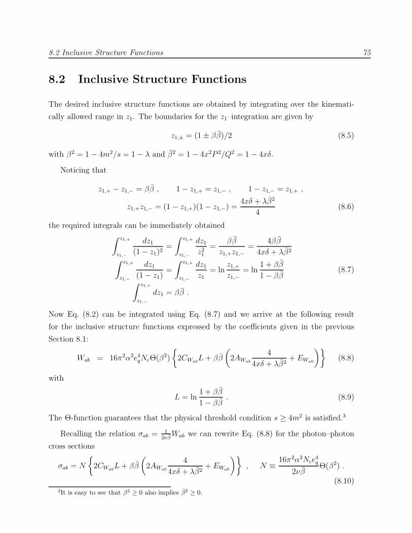
8.2 Inclusive Structure Functions 75

8.2 Inclusive Structure Functions

The desired inclusive structure functions are obtained by integrating over the kinemati-

cally allowed range in z1. The boundaries for the z1–integration are given by

z1,± = (1± ββ)/2 (8.5)

with β2 = 1− 4m2/s = 1− λ and β2 = 1− 4x2P 2/Q2 = 1− 4xδ.

Noticing that

z1,+ − z1,− = ββ , 1− z1,+ = z1,− , 1− z1,− = z1,+ ,

z1,+z1,− = (1− z1,+)(1− z1,−) =4xδ + λβ2

4(8.6)

the required integrals can be immediately obtained∫ z1,+

z1,−

dz1(1− z1)2

=

∫ z1,+

z1,−

dz1z21

=ββ

z1,+z1,−=

4ββ

4xδ + λβ2

∫ z1,+

z1,−

dz1(1− z1)

=

∫ z1,+

z1,−

dz1z1

= lnz1,+z1,−

= ln1 + ββ

1− ββ∫ z1,+

z1,−

dz1 = ββ .

(8.7)

Now Eq. (8.2) can be integrated using Eq. (8.7) and we arrive at the following result

for the inclusive structure functions expressed by the coefficients given in the previous

Section 8.1:

Wab = 16π2α2e4qNcΘ(β2)

{2CWab

L+ ββ

(2AWab

4

4xδ + λβ2+ EWab

)}(8.8)

with

L = ln1 + ββ

1− ββ. (8.9)

The Θ-function guarantees that the physical threshold condition s ≥ 4m2 is satisfied.3

Recalling the relation σab =1

2νβWab we can rewrite Eq. (8.8) for the photon–photon

cross sections

σab = N

{2CWab

L+ ββ

(2AWab

4

4xδ + λβ2+ EWab

)}, N ≡

16π2α2Nce4q

2νβΘ(β2) .

(8.10)3It is easy to see that β2 ≥ 0 also implies β2 ≥ 0.

8.2 Inclusive Structure Functions 76

Inserting the coefficients given in Eq. (8.4) into Eq. (8.10) one obtains the final result for

the doubly virtual box γ⋆(Q2)γ⋆(P 2) → qq in leading order:

σTT =N

4π

1

β5

{[1− 2x(1− x)− 2δ(1− δ)− 4xδ(x2 + δ2) + 8x2δ2

[1 + (1− x− δ)2

]

+ λβ2(1− x− δ)2 − 1

2λ2β4(1− x− δ)2

]L+ ββ

[4x(1− x)− 1

+ 4δ(1− δ)− 8xδ(1− x2 − δ2)− (4xδ + λβ2)(1− x− δ)2 − 4xδβ4

4xδ + λ β2

]}

σLT =N

4π

4

β5(1− x− δ)

{x

[−1

2λ β2

(1− 2δ(1 + x− δ)

)− 2δ

(−1 + 2x+ 2δ

− 2xδ(1 + x+ δ))]

L+ ββ

[x(1− 6δ + 6δ2 + 2xδ) + δβ2 4xδ

4xδ + λ β2

]}

σTL = σLT[x ↔ δ]

σLL =N

4π

16

β5xδ(1− x− δ)2

{(1 + 2xδ)L− 2ββ

6xδ + λβ2

4xδ + λβ2

}

τTT =N

4π

1

β5

{[1

2xδ(1− 2x(1− x)− 2δ(1− δ) + 2xδ(1− 2x− 2δ − x2 − δ2 + 6xδ)

)

− 2λβ2(1− x− δ)(x+ δ − 2xδ(1 + x+ δ)

)− 1

2λ2β4(1− x− δ)2

]L

− ββ

[(1− x− δ)2(4xδ + λβ2) + 2(x+ δ − 4xδ)2

]}

τTL =N

4π

2

β5

√xδ(1− x− δ)

{[2x+ 2δ − 4xδ(3− x− δ)− λβ2(1− x− δ)

]L

+ ββ(1− 3x− 3δ + 8xδ)

}

8.3 Comparison with Present e+e− Virtual Photon Data 77

τ aTT =N

4π

1

β3

{(2x− 1)(1− 2δ)L+ ββ

[ −4xδβ2

4xδ + λβ2+ 3− 4x− 4δ + 4xδ

]}

τ aTL =N

4π

4

β3

√xδ(1− x− δ)

{2xδL− ββ

4xδ

4xδ + λβ2

}(8.11)

This recalculation is in agreement with the results of Ref. [82] (with Nce4q → 1) with

exception of a relative sign between the part containing the logarithm L and the part

proportional to ββ in τ aTL4.

A derivation of various important limits of the doubly virtual box expressions in (8.11)

can be found in App. C.

8.3 Comparison with Present e+e− Virtual Photon

Data

We will now compare our LO–box expressions with present e+e− virtual photon data.

The physically measured effective structure function in the Bjorken limit is [82, 85, 90]

Feff(x; Q2, y1; P

2, y2) =Q2

4π2α

1

β

[σTT + ε(y1)σLT + ε(y2)σTL + ε(y1)ε(y2)σLL

](8.12)

where the kinematical variables have been given in Eqs. (7.2) and (7.1) and where ε(yi)

are the ratios of longitudinal to transverse photon fluxes,

ε(yi) = 2(1− yi)/[1 + (1− yi)2] . (8.13)

Furthermore, the photon–photon cross sections σab = σab(x,Q2, P 2) with a =

(L,T), b = (L,T) have been defined in (7.20). In the following we shall consider the

kinematical region yi ≪ 1 relevant for double–tag experiments [105, 106] performed thus

far where Eq. (8.12) reduces to

Feff(x,Q2, P 2) ≃ Q2

4π2α

1

β

[σTT + σLT + σTL + σLL

]. (8.14)

4This relative sign has also been noted in [104] where in addition the overall sign in τTL is different.Concerning the latter, we agree with the results of [82].

8.3 Comparison with Present e+e− Virtual Photon Data 78

Recalling the general definitions of the structure functions of spin–averaged, transverse

and longitudinal target photons in Sec. 7.2 we can finally write

Feff(x,Q2, P 2) ≃ F

γT(P 2)2 (x,Q2) + F

γL(P2)

2 (x,Q2)

= F<γ(P 2)>2 (x,Q2) +

3

2F

γL(P2)

2 (x,Q2) . (8.15)

So far, our results are entirely general.

We shall furthermore introduce the decomposition

σab = σℓab + σh

ab (8.16)

with σℓ(h)ab denoting the light (heavy) quark q = u, d, s (h = c, b, t) contributions. The

light u, d, s contributions to σℓab are obtained from Eq. (8.11) by setting m ≡ mq =

0 (λ = 0) and summing over q = u, d, s. (Note that the box expressions involving a

real photon, γ∗(Q2) γ (P 2 = 0) → qq, require on the contrary a finite regulator mass

m ≡ mq 6= 0; here one usually chooses mq to be, somewhat inconsistently, a constant,

i.e. Q2–independent effective constituent mass, mq ≃ 0.3 GeV.) For each heavy quark

flavor h = c, b, t the heavy contribution σhab in (8.16) is obtained from Eq. (8.11) with

eq ≡ eh and m ≡ mh. Only charm gives a non–negligible contribution for which we choose

mc = 1.4 GeV throughout.

Finally, it is instructive to recall the asymptotic results of our virtual (P 2 6= 0) box

expressions for the light q = u, d, s quarks derived from (8.11) in the Bjorken limit

P 2/Q2 ≪ 1, see App. C.2:

σℓTT ≃ Nc(Σe

4q)4πα2

Q2x

{[x2 + (1− x)2] ln

Q2

P 2x2+ 4x(1− x)− 2

}

σℓTL ≃ σℓ

LT ≃ Nc(Σe4q)4πα2

Q2x [4x(1− x)]

σℓLL ≃ 0 . (8.17)

We now turn to a comparison of the effective structure function Feff obtained in lowest

order perturbation theory with all presently available e+e− data of PLUTO [106] and the

recent one of LEP–L3 [105]. In addition to the full LO–box calculation of Feff (solid line)

we show the ’asymptotic box’ results (dotted line) where the light quark contributions

have been calculated according to (8.17). As can be seen the ’full’ and the ’asymptotic’

curves are very similar and coincide in Fig. 8.4 over the entire x–range. Furthermore,

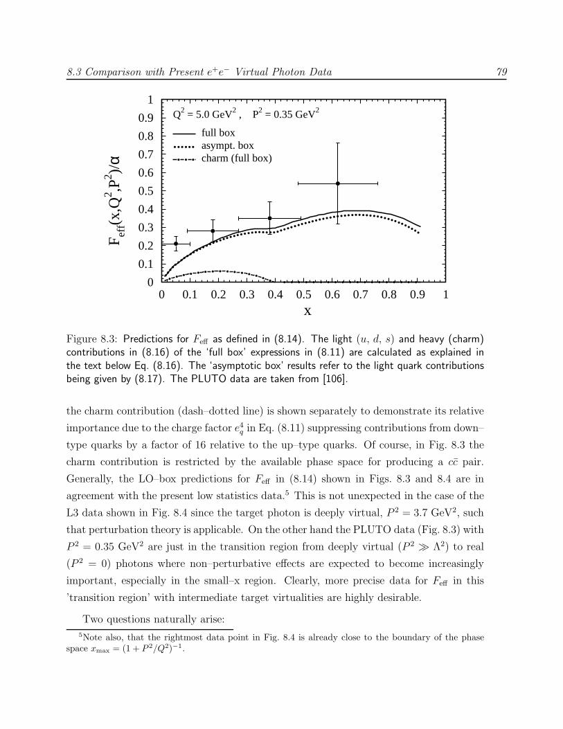
8.3 Comparison with Present e+e− Virtual Photon Data 79

Q2 = 5.0 GeV2 , P2 = 0.35 GeV2F ef

f(x,

Q2 ,P

2 )/α

x

full boxasympt. boxcharm (full box)

0

0.1

0.2

0.3

0.4

0.5

0.6

0.7

0.8

0.9

1

0 0.1 0.2 0.3 0.4 0.5 0.6 0.7 0.8 0.9 1

Figure 8.3: Predictions for Feff as defined in (8.14). The light (u, d, s) and heavy (charm)contributions in (8.16) of the ‘full box’ expressions in (8.11) are calculated as explained inthe text below Eq. (8.16). The ‘asymptotic box’ results refer to the light quark contributionsbeing given by (8.17). The PLUTO data are taken from [106].

the charm contribution (dash–dotted line) is shown separately to demonstrate its relative

importance due to the charge factor e4q in Eq. (8.11) suppressing contributions from down–

type quarks by a factor of 16 relative to the up–type quarks. Of course, in Fig. 8.3 the

charm contribution is restricted by the available phase space for producing a cc pair.

Generally, the LO–box predictions for Feff in (8.14) shown in Figs. 8.3 and 8.4 are in

agreement with the present low statistics data.5 This is not unexpected in the case of the

L3 data shown in Fig. 8.4 since the target photon is deeply virtual, P 2 = 3.7 GeV2, such

that perturbation theory is applicable. On the other hand the PLUTO data (Fig. 8.3) with

P 2 = 0.35 GeV2 are just in the transition region from deeply virtual (P 2 ≫ Λ2) to real

(P 2 = 0) photons where non–perturbative effects are expected to become increasingly

important, especially in the small–x region. Clearly, more precise data for Feff in this

’transition region’ with intermediate target virtualities are highly desirable.

Two questions naturally arise:

5Note also, that the rightmost data point in Fig. 8.4 is already close to the boundary of the phasespace xmax = (1 + P 2/Q2)−1.

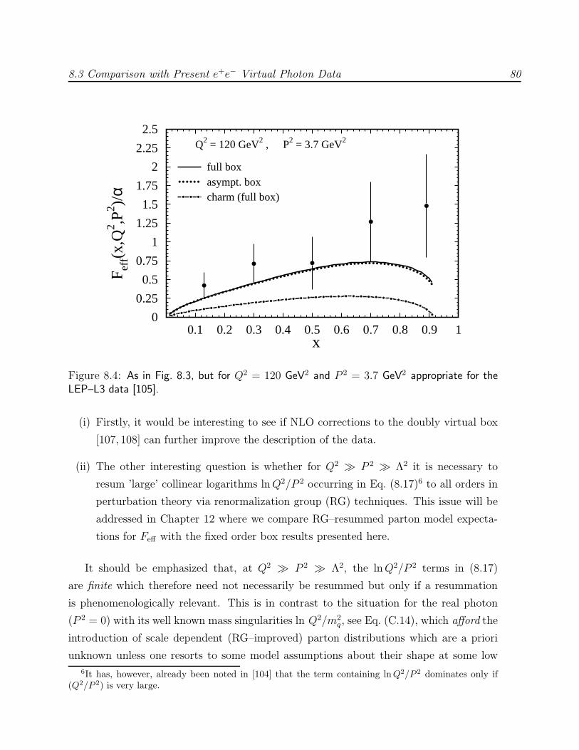
8.3 Comparison with Present e+e− Virtual Photon Data 80

Q2 = 120 GeV2 , P2 = 3.7 GeV2

F eff(

x,Q

2 ,P2 )/

α

x

full boxasympt. boxcharm (full box)

0

0.25

0.5

0.75

1

1.25

1.5

1.75

2

2.25

2.5

0.1 0.2 0.3 0.4 0.5 0.6 0.7 0.8 0.9 1

Figure 8.4: As in Fig. 8.3, but for Q2 = 120 GeV2 and P 2 = 3.7 GeV2 appropriate for theLEP–L3 data [105].

(i) Firstly, it would be interesting to see if NLO corrections to the doubly virtual box

[107, 108] can further improve the description of the data.

(ii) The other interesting question is whether for Q2 ≫ P 2 ≫ Λ2 it is necessary to

resum ’large’ collinear logarithms lnQ2/P 2 occurring in Eq. (8.17)6 to all orders in

perturbation theory via renormalization group (RG) techniques. This issue will be

addressed in Chapter 12 where we compare RG–resummed parton model expecta-

tions for Feff with the fixed order box results presented here.

It should be emphasized that, at Q2 ≫ P 2 ≫ Λ2, the lnQ2/P 2 terms in (8.17)

are finite which therefore need not necessarily be resummed but only if a resummation

is phenomenologically relevant. This is in contrast to the situation for the real photon

(P 2 = 0) with its well known mass singularities ln Q2/m2q , see Eq. (C.14), which afford the

introduction of scale dependent (RG–improved) parton distributions which are a priori

unknown unless one resorts to some model assumptions about their shape at some low

6It has, however, already been noted in [104] that the term containing lnQ2/P 2 dominates only if(Q2/P 2) is very large.

8.3 Comparison with Present e+e− Virtual Photon Data 81

resolution scale (see, e.g., [6] and the recent reviews [89, 90]).

In the next chapter we present the necessary theoretical background for describing

(virtual) photon structure functions within the QCD–improved (RG–improved) parton

model.

Chapter 9

The Partonic Structure of Real andVirtual Photons: TheoreticalFramework

The following chapters are mainly devoted to an analysis of the structure of the (real and

virtual) photon within the framework of the renormalization group (RG) improved parton

model. It is the main purpose here to provide the necessary theoretical background for

these phenomenological studies where special emphasis is laid on a unified treatment of

both real (P 2 = 0) and virtual (P 2 6= 0) photons.

After motivating our unified approach in Sec. 9.1 we turn to a detailed description of

the unpolarized photon structure functions within the QCD improved parton model in

Sec. 9.2. This section provides the complete technical framework for our analysis of the

parton content of real and virtual photons in Chapter 11. In Sec. 9.3 we deal with the

RG–based evolution equations for photonic parton distributions and their solutions. For

completeness, we discuss boundary conditions for a deeply virtual target photon and from

the evolution equations we derive leading and next–to–leading order expressions for the

momentum sum carried by the photon’s quark and gluon densities. Finally, in Sec. 9.4

we briefly discuss how to include contributions from longitudinal target photons.

9.1 Introduction

We have seen in Chapter 7 that the cross section for the process ee → eeX factorizes in the

Bjorken limit into fluxes of transversely (longitudinally) polarized photons and the cross

9.1 Introduction 83

qe(p1)

e(p2)p

Figure 9.1: Deep inelastic electron–photon scattering (cf. Fig. 7.4) in the parton model wherethe target photon is produced by the bremsstrahlung process. According to the factorizationtheorems [68, 109] the eγ cross section factorizes into ’long distance’ (non–perturbative) partondistributions (grey oval) describing the internal structure of the photon and ’short distance’(perturbatively calculable) electron–parton subprocesses (black oval).

sections for deep inelastic scattering on these transverse (longitudinal) target photons.

The deep inelastic scattering cross sections can in turn be expressed in terms of two

independent structure functions, e.g. FγT(P

2)2 (x,Q2) and F

γT(P2)

L (x,Q2) (FγL(P

2)2 (x,Q2),

FγL(P

2)L (x,Q2)).

Furthermore, in Chapter 8 we have obtained these structure functions (or the effective

structure function Feff) according to a perturbative calculation of the doubly virtual box

γ⋆(Q2)γ⋆(P 2) → qq in lowest order perturbation theory. As has been discussed there in

the deeply virtual case P 2 ≫ Λ2 (where Λ is a hadronic scale) perturbation theory is

expected to be reliable and we have compared these fixed order ’box results’ F boxeff with

presently available e+e− data leaving the open question if resummations of the collinear

logarithms lnQ2/P 2 might further improve the situation. On the other hand, for P 2 . Λ2

the perturbatively calculated structure functions (cross sections) are invalidated by non–

perturbative (long–distance) mass singularities which have to be subtracted. This problem

can be consistently solved by turning to a parton model description (see Fig. 9.1): Since

we are considering the Bjorken limit, the structure functions can be described in terms

of photonic parton distributions, quite similar to the hadronic case where factorization

theorems [68, 109] state that the structure functions are given by convolutions of par-

ton distributions with Wilson coefficient functions. The parton distributions contain the

long–distance part of the cross section and therefore can (in general) not be calculated

perturbatively and have to be fixed by experimental information or model assumptions.

On the other hand the coefficient functions involve only short–distance physics and are

9.1 Introduction 84

calculable in perturbation theory. The main value of this approach lies in the fact that

the parton distribution functions (PDFs) are universal, i.e. do not depend on the partic-

ular hard scattering subprocess. Once fixed by experimental information from, e.g., deep

inelastic electron–photon scattering the PDF’s can be used to make predictions for other

processes, for example photo–and electroproduction of jets or heavy quarks.

Due to QED gauge invariance the contributions (structure functions, cross sections)

from longitudinal target photons have to vanish in the real photon limit (P 2 → 0). More

specifically, they are suppressed by a factor P 2 divided by a typical hadronic scale, say

P 2/mρ2 [82], for not too large virtualities P 2 of the target photon. Therefore, we will

mainly focus on the structure functions of transverse target photons. The contributions

from longitudinal photon targets will be considered at the end of this chapter. In the

following we can therefore drop the index T and use instead γ(P 2) to denote transverse

target photons. Our main interest will lie on Fγ(P 2)2 (x,Q2) since up to now the cross

section has been measured only for small values of y where the contribution of FL(∝ y2)

is negligible.

The following parton content can be assigned to a transverse photon target:

qγ(P2)(x,Q2), gγ(P

2)(x,Q2), and Γγ(P 2)(x,Q2) where q and g are the photonic analogues

of the usual quark and gluon parton distributions inside hadrons. In addition the tar-

get photon also contains an elementary photon–parton Γγ(P 2) reflecting the fact that the

photon is a genuinely elementary particle which can directly enter a partonic subprocess.

As usual in a massless parton model approach (justified by the factorization theorems

[68, 109]) the partonic subprocesses are calculated with on–shell partons partly due to the

P 2/Q2 power suppression of effects invoked by the off–shellness of the partons (which is

of the order O(P 2)). While this is quite familiar for the quarks and gluons the latter

rule also refers to the photon–parton Γγ(P 2)(x,Q2) in the target photon, i.e., the ’direct’

subprocesses, e.g., γ⋆(Q2)Γγ(P 2) → qq have to be calculated with P 2 = 0 (cf. rule (ii) in

[6]). Consequently we can use the same (massless) short distance coefficient functions

in our calculations irrespective of P 2. All effects due to a non–zero target virtuality are

entirely taken care of by the P 2–dependence of the parton distributions f γ(P 2) (and by

the Weizsacker–Williams flux factors) which of course have to be given in the same fac-

torization scheme as the coefficient functions in order to obtain a physically meaningful,

i.e. factorization scheme independent, result. By construction a physically smooth behav-

ior in P 2 (including a smooth transition to the real photon case P 2 = 0) of the observable

9.2 Photon Structure Functions in the QCD–Improved Parton Model 85

structure functions can be automatically achieved by demanding a smooth behavior of

the boundary conditions for the parton distributions.

The heavy quark contributions deserve special care due to the additional scale mh

provided by the heavy quark mass. In this case terms P 2/m2h are possibly not negligible

and have to be kept in the heavy quark coefficient functions. We will come back to this

point in Sec. 9.2.2.

9.2 Photon Structure Functions in the QCD–

Improved Parton Model

We shall introduce the decomposition

Fγ(P 2)i (x,Q2) = F

γ(P 2)i,ℓ (x,Q2) + F

γ(P 2)i,h (x,Q2) (9.1)

with Fγ(P 2)i,ℓ (h) denoting contributions with light quarks q = u, d, s (heavy quarks h = c, b, t)

in the final state. In NLO(MS) Fγ(P 2)2,ℓ (x,Q2) and F

γ(P 2)1,ℓ (x,Q2) are given by the following

expressions:

1

xF

γ(P 2)2,ℓ (x,Q2) =

∑

q=u,d,s

e2q

{qγ(P

2)(x,Q2) + q γ(P 2)(x,Q2) +αs(Q

2)

2π

×[Cq,2 ⊗ (q + q)γ(P

2) + 2Cg,2 ⊗ gγ(P2)]+

α

πe2qCγ,2(x)

}(9.2)

Fγ(P 2)1,ℓ (x,Q2) =

1

2

∑

q=u,d,s

e2q

{qγ(P

2)(x,Q2) + q γ(P 2)(x,Q2) +αs(Q

2)

2π

×[Cq,1 ⊗ (q + q)γ(P

2) + 2Cg,1 ⊗ gγ(P2)]+

α

πe2qCγ,1(x)

}(9.3)

where ⊗ denotes the usual convolution integral of two functions f and g defined on the

interval [0, 1]:

(f ⊗ g)(x) =

∫ 1

0

dx1

∫ 1

0

dx2f(x1)g(x2)δ(x− x1x2) =

∫ 1

x

dz

zf(z)g(x/z) . (9.4)

Here q γ(P 2)(x,Q2) = qγ(P2)(x,Q2) and gγ(P

2)(x,Q2) provide the so–called ‘resolved’ con-

tributions of γ(P 2) to Fγ(P 2)i with the MS coefficient functions [30, 48, 54]

Cq,2(x) = Cq,1(x) +4

32x

=4

3

[1 + x2

1− x

(ln

1− x

x− 3

4

)+

1

4(9 + 5x)

]

+

9.2 Photon Structure Functions in the QCD–Improved Parton Model 86

Cg,2(x) = Cg,1(x) +1

24x(1− x)

=1

2

[(x2 + (1− x)2

)ln

1− x

x+ 8x(1− x)− 1

], (9.5)

while Cγ,2,1 in (9.2) provides the ‘direct’ contribution as calculated according to the ‘box’

diagram γ∗(Q2)γ → qq [110]:

Cγ,i(x) =3

(1/2)Cg,i(x) (9.6)

with i = 1, 2. The convolution with the [ ]+ distribution can be evaluated using, for

example, Eq. (A.21) in Ref. [57]:

f+ ⊗ g =

∫ 1

x

dy

yf

(x

y

)[g(y)− x

yg(x)

]− g(x)

∫ x

0

dyf(y) . (9.7)

The coefficient functions Cq,L and Cg,L for the longitudinal structure function Fγ(P 2)L =

Fγ(P 2)2 − 2xF

γ(P 2)1 may be deduced from Eqs. (9.5) and (9.6) and are given by [111]:

Cq,L(x) =4

32x , Cg,L(x) =

1

24x(1− x) , Cγ,L(x) =

3

(1/2)Cg,L(x) . (9.8)

9.2.1 Scheme Choice

In order to avoid the usual instabilities encountered in NLO(MS) in the large–x region due

to the ln(1−x) term in Cγ,2(x) in Eq. (9.6), we follow Ref. [96, 112] and absorb such terms

into the photonic MS quark distributions in Eq. (9.2): this results in the so–called DISγ

factorization scheme which originally has been introduced for real photons by absorbing

the entire ’direct’ Cγ,2 term appearing in Eq. (9.2) into the NLO(MS) quark densities

qγ(P2)(x,Q2) = qγ(P

2)(x,Q2), i.e.

(q + q)γ(P 2)DISγ

= (q + q)γ(P 2)

MS+ e2q

α

πCγ,2(x)

gγ(P 2)DISγ

= gγ(P 2)

MS

(9.9)

with Cγ,2(x) given by Eq. (9.6). How much of the ‘finite’ terms in Eq. (9.6) is absorbed

into the MS distributions in Eq. (9.9), is of course arbitrary and a matter of convention

[113]. Since such different conventions [113, 114] differ by terms of higher order and turn

out to be of minor importance for our quantitative results to be discussed in Chap. 11, we

prefer to stick to the original DISγ scheme [96, 112] as defined in Eq. (9.9). Furthermore,

9.2 Photon Structure Functions in the QCD–Improved Parton Model 87

the redefinition of the parton densities in Eq. (9.9) implies that the NLO(MS) splitting

functions k(1)q,g(x) of the photon into quarks and gluons, appearing in the inhomogeneous

NLO RG evolution equations for f γ(P 2)(x,Q2), have to be transformed according to [96,

112, 115]

k(1)q |DISγ = k(1)

q − e2q P(0)qq ⊗ Cγ,2

k(1)g |DISγ = k(1)

g − 2∑

q

e2q P(0)gq ⊗ Cγ,2

(9.10)

where

k(1)q (x) =

1

23e2q

4

3

{−(1− 2x) ln2 x− (1− 4x) ln x+ 4 ln(1− x)− 9x+ 4

+[x2 + (1− x)2

] [2 ln2 x+ 2 ln2(1− x) + 4 ln x− 4 ln x ln(1− x)

− 4 ln(1− x) + 10− 2

3π2

]}

k(1)g (x) = 3

∑

q

e2q4

3

{−2(1 + x) ln2 x− (6 + 10x) ln x+

4

3x+

20

3x2 + 8x− 16

}(9.11)

with k(1)q referring to each single (anti)quark flavor. The LO splitting functions are given

by P(0)qq = 4

3

(1+x2

1−x

)+and P

(0)gq = 4

3[1 + (1− x)2] /x.

In NLO the expression for Fγ(P 2)2 in the above DISγ factorization scheme is given by

retaining the Cq,2, Cg,2 terms while dropping the destabilizing Cγ,2 term in Eq. (9.2), which

has already been absorbed into the quark densities according to Eq. (9.9). Similarly,

Cq,1 and Cg,1 remain unchanged while Cγ,1 has to be modified according to CDISγγ,1 =

CMSγ,1 − CMS

γ,2 = −12x(1− x).

The LO expression for Fγ(P 2)i (i = 1, 2) are obviously entailed in Eq. (9.2) by simply

dropping all NLO terms proportional to Cq,i, Cg,i as well as Cγ,i.

9.2.2 Heavy Flavor Contributions

The photonic quark distributions discussed thus far and which appear in Eq. (9.2) are

adequate for the f = 3 light u, d, s flavors. Since heavy quarks h = c, b, t will not be

considered as ‘light’ partons in the photon (as in the case of the proton [26] and the pion

[5, 116]), their contributions to Fγ(P 2)i (i = 1, 2, L) have to be calculated in fixed order

9.2 Photon Structure Functions in the QCD–Improved Parton Model 88

q

p

h

h

+ crossed

(a)

q

p

h

h

+ crossed

(b)

Figure 9.2: Direct (a) and resolved (b) contribution of a heavy quark h in deep inelasticeγ(P 2) scattering.

perturbation theory. The heavy quark contribution consist of two parts, a ’direct’ one

and a ’resolved’ one as depicted in Fig. 9.2:

Fγ(P 2)i,h = F

γ(P 2),diri,h + F

γ(P 2),resi,h . (9.12)

The ‘direct’ contribution derives from the box–diagram γ∗(Q2) γ → hh expression, i.e. the

usual Bethe–Heitler cross section [117]

1

xF

γ(P 2),dir2,h (x,Q2) = 3 e4h

α

πθ(β2)

{β

[8x(1− x)− 1− x(1 − x)

4m2h

Q2

]

+

[x2 + (1− x)2 + x(1− 3x)

4m2h

Q2− x2 8m

4h

Q4

]ln

1 + β

1− β

}

2Fγ(P 2),dir1,h (x,Q2) = 3 e4h

α

πθ(β2)

{β

[4x(1− x)− 1− x(1 − x)

4m2h

Q2

]

+

[x2 + (1− x)2 + x(1− x)

4m2h

Q2− x2 8m

4h

Q4

]ln

1 + β

1− β

}(9.13)

where β2 ≡ 1− 4m2h/W

2 = 1− 4m2hx/(1−x)Q2. A similar expression holds for the longi-

tudinal structure function [111] FL ≡ F2−2xF1. The ‘resolved’ heavy quark contribution

to Fγ(P 2)i has to be calculated via γ∗(Q2)g → hh and is given by [111]

Fγ(P 2),res2,h (x,Q2) =

∫ 1

zmin

dz

zzgγ(P

2)(z, µ2F ) f

γ∗(Q2)g→hh2

(xz, Q2

)

Fγ(P 2),res1,h (x,Q2) =

∫ 1

zmin

dz

zgγ(P

2)(z, µ2F ) f

γ∗(Q2)g→hh1

(xz, Q2

)(9.14)

9.3 Q2–Evolution 89

where 1xfγ∗(Q2)g→hh2 (x,Q2) and 2f

γ∗(Q2)g→hh1 (x,Q2) are given by Eq. (9.13) with e4hα →

e2hαs(µ2F )/6, zmin = x(1 + 4m2

h/Q2) and µ2

F ≃ 4m2h [18]1. To ease the calculations we

shall keep these LO expressions in Eqs. (9.13) and (9.14) also in NLO, since the full

NLO expressions for heavy quark production [119] turn out to be a small correction to

the already not too sizeable (at most about 20%) contribution in LO. Notice that such

small corrections are not larger than ambiguities due to different choices for mh and for

the factorization scale µF . For our purposes it is sufficient to include only the charm

contributions which will be calculated using mc = 1.4 GeV.

As already mentioned in the introduction the heavy quark contributions deserve special

care due to the additional scale mh provided by the heavy quark mass. For general

P 2(≪ Q2) terms P 2/m2h are not always power–suppressed and have to be kept in the

heavy quark coefficient functions. The corresponding ’direct’ and ’resolved’ heavy quark

contributions can be found in Eqs. (18) and (19) of Ref. [111].

9.3 Q2–Evolution

9.3.1 Evolution Equations

As motivated in Sec. 9.1 a transverse hadronic photon can be described by its partonic

quark, gluon and photon content denoted by qγ(P 2)i (x,Q2) (i = 1, . . . , f) with q1 = u,

q2 = d, q3 = s and so on2, gγ(P2)(x,Q2), and Γγ(P 2)(x,Q2). The general evolution equations

for these parton densities are given by (suppressing the x– and Q2–dependence)

dqγ(P 2)i

d lnQ2= Pqiγ ⊗ Γγ(P 2) + 2

f∑

k=1

Pqiqk ⊗ qγ(P 2)k + Pqig ⊗ gγ(P

2)

dgγ(P2)

d lnQ2= Pgγ ⊗ Γγ(P 2) + 2

f∑

k=1

Pgqk ⊗ qγ(P 2)k + Pgg ⊗ gγ(P

2) (9.15)

dΓγ(P 2)

d lnQ2= Pγγ ⊗ Γγ(P 2) + 2

f∑

k=1

Pγqk ⊗ qγ(P 2)k + Pγg ⊗ gγ(P

2)

1An alternative choice would be µ2F = Q2 + 4m2

h [118] which satisfies the requirement µ2F ≫ P 2 also

for large P 2.2Note that due to charge conjugation invariance q

γ(P 2)i (x,Q2) = q

γ(P 2)i (x,Q2).

9.3 Q2–Evolution 90

where f denotes the number of active (massless) quark flavors. The evolution kernels Pij

are generalized splitting functions

Pij(x, α, αs) =∑

l,m=0

αlαms

(2π)l+mP(l,m)ij (x), (9.16)

with Pqiqk being the average of the quark–quark and antiquark–quark splitting functions.

Note that terms due to photon radiation from the quark line are taken into account in

Eq. (9.15) as it must be in order to guarantee momentum conservation (see the erratum

to [120]).

Since the electromagnetic coupling constant α ≪ 1 we can safely neglect terms of

order O(α2) in Eq. (9.15)3. Noticing that qγ(P2) and gγ(P

2) are already of order O(α) we

can take l = 0 in all generalized splitting functions in (9.16) which are multiplied by qγ(P2)

or gγ(P2) such that the functions Pij reduce in this case to the conventional QCD splitting

functions Pij(x, αs). On the other hand in Pqiγ, Pgγ and Pγγ the contributions with l = 0

obviously vanish such that the only contribution to order O(α) comes from setting l = 1

in Eq. (9.16) in this case. Furthermore, the terms proportional to Pγqk and Pγg are of

the order O(α2) and can be dropped such that the evolution equation for the photon

distribution decouples and can be solved separately as will be discussed in Sec. 9.3.5.

Here it suffices to know the photon density at order α0 only in order to obtain the quark

and gluon densities in Eq. (9.15) and the structure functions in Eq. (9.2) consistently to

order O(α). At 0th order, however, no splitting is possible and the photon carries its full

momentum with probability one: Γγ(P 2)(x,Q2) = δ(1− x) +O(α).

Therefore, Eq. (9.15) can be reduced to the following inhomogeneous evolution equa-

tions for the quark and gluon content of the photon [120]:

dqiγ(P 2)

d lnQ2= kqi + 2

f∑

k=1

Pqiqk ⊗ qkγ(P 2) + Pqig ⊗ gγ(P

2)

dgγ(P2)

d lnQ2= kg + 2

f∑

k=1

Pgqk ⊗ qkγ(P 2) + Pgg ⊗ gγ(P

2) (9.17)

where we have utilized the standard notation kqi ≡ Pqiγ, kg ≡ Pgγ for the photon–quark

and photon–gluon splitting functions. The splitting functions Pij(x, αs) are presently

known to next–to–leading order in αs and can be found in [112, 121, 122].

3For this reason we can also neglect the running of α(Q2) and use α ≃ 1/137.

9.3 Q2–Evolution 91

The Q2–evolution is most conveniently treated in the Mellin moment space where the

convolutions turn into ordinary products: (a ⊗ b)(x) → (a ⊗ b)n = anbn where the n–th

Mellin moment of a function f(x,Q2) is defined by

fn(Q2) =

∫ 1

0

dx xn−1f(x,Q2) . (9.18)

Hence the evolution of n–moments is governed by a set of ordinary coupled differential

equations which can be solved analytically [112].

In order to decouple the evolution equations as far as possible we introduce flavor

non–singlet (NS) quark combinations:

qγ(P 2)NS,ℓ = 2

[j∑

i=1

qiγ(P 2) − jqj

γ(P 2)

](9.19)

with i, j = 1, . . . , f and the group theoretical index ℓ = j2 − 1. Thus, for three active

flavors (u, d, s) we have two non–vanishing NS combinations qNS,3 = 2(u− d) and qNS,8 =

2(u+ d− 2s). Furthermore, we define a singlet (S) vector which helps to write the singlet

evolution equations and their solutions in a compact matrix form:

~qγ(P 2)S =

(Σγ(P 2)

gγ(P2)

), Σγ(P 2) = 2

f∑

i=1

qiγ(P 2) . (9.20)

We wish to make an expansion of the solutions of the evolution equations and even-

tually of the structure functions in terms of αs. For this reason the evolution equations

will be rewritten as differential equations in αs with help of the renormalization group

equation for the strong coupling constant:

dαs

d lnQ2= − β0

4πα2s(Q

2)− β1

(4π)2α3s(Q

2) +O(α4s) (9.21)

with β0 = 11 − (2/3)f and β1 = 102 − (38/3)f . Expanding the splitting functions

in αs in a form which can be generically written as P = αs

2π(P (0) + αs

2πP (1) + . . . ) and

k = α2π(k(0) + αs

2πk(1) + . . . ), respectively, and neglecting terms of the order O(α2

s) the

inhomogeneous evolution equations can be brought into the following form:

d

dαsqγ(P 2),nNS,ℓ = − α

α2s

2

β0k(0)nℓ − α

αs

1

πβ0

(k(1)nℓ − β1

2β0k(0)nℓ

)

−[1

αs

2

β0P (0)nqq +

1

πβ0

(P

(1)n+ − β1

2β0P (0)nqq

)]qγ(P 2),nNS,ℓ

9.3 Q2–Evolution 92

d

dαs

~qγ(P 2),nS = − α

α2s

2

β0

~k(0)n − α

αs

1

πβ0

(~k(1)n − β1

2β0

~k(0)n

)

−[1

αs

2

β0P (0)n +

1

πβ0

(P (1)n − β1

2β0P (0)n

)]~qγ(P 2),nS . (9.22)

Here ~k(0)n and ~k(1)n denote the LO and NLO photon–to-parton splitting functions in the

singlet sector: ~kn =(knΣ, k

ng

)Twith kn

Σ = 2∑f

i=1 knqiwhile k

(0)nℓ and k

(1)nℓ are the LO and

NLO parts of the non–singlet combination knℓ = 2

[∑ji=1 k

nqi− jkn

qj

]. Furthermore, P (0)n

and P (1)n refer to LO and NLO 2 × 2 matrices of one– and two–loop splitting functions

whereas P(1)n+ and P

(0)nqq occurring in the NS equation are scalar functions. The complete

set of LO and NLO (non–)singlet splitting functions can be found, e.g., in [112, 123].

9.3.2 Analytic Solutions

The general solutions of the inhomogeneous evolution equations (9.22) are formally iden-

tical to the ones of a real photon [112] and can be written, as usual, as a sum of a

(’pointlike’) particular solution qpl of the inhomogeneous problem and a general solution

qhad of the homogeneous (’hadronic’) equations :

q = qpl + qhad , q = qγ(P 2),nNS,ℓ , ~q

γ(P 2),nS , q γ(P 2),n, . . . . (9.23)

The particular solution is not unique and we fix it by the condition qpl(Q20) ≡ 0 at the

reference scale Q20.

The NLO ’pointlike’ (inhomogeneous) flavor–singlet solution is given by [111, 112]

~qγ(P 2),nS,pl (Q2) =

2π

αs(Q2)

(1 +

αs(Q2)

2πUn

)[1− L1+dn

] 1

1 + dn

α

πβ0

~k(0)n

+[1− Ldn

] 1

dn

α

πβ0

(~k(1)n − β1

2β0

~k(0)n − Un~k(0)n

)(9.24)

where dn ≡ −(2/β0)P(0)n, L ≡ αs(Q

2)/αs(Q20) and the 2 × 2 NLO evolution matrix

U is fixed through the commutation relation [Un, P (0)n] = β0

2Un + P (1)n − β1

2β0P (0)n [30,

112, 123]. The NLO ’hadronic’ (homogeneous) solution depending on input distributions

~qγ(P 2),nS,had (Q2

0) = ~qγ(P 2),nS (Q2

0) which will be specified in Chapter 11 is given by [111, 112]

~qγ(P 2),nS,had (Q2) =

[Ldn +

αs(Q2)

2πUnLdn − αs(Q

20)

2πLdnUn

]~qγ(P 2),nS,had (Q2

0) . (9.25)

9.3 Q2–Evolution 93

The LO results are obviously entailed in these expressions by simply dropping all higher or-

der terms (β1, ~k(1)n, U). The non–singlet solutions can be easily obtained from Eqs. (9.24)

and (9.25) by the obvious replacements P (0) → P(0)qq , P (1) → P

(1)+ , ~k → kℓ together with

U → U+,ℓ = − 2β0

(P(1)+ − β1

2β0P(0)qq

)[112, 123].

Note that the solutions (9.24) and (9.25) are valid for a fixed number f of active flavors.

Evoluting beyond an MS ’threshold’, set by the heavy quark masses mc, mb and mt, the

number of active flavors has to be increased by one, i.e., f → f + 1 in the calculation of

αs. The evolution of α(f)s (Q2), corresponding to a number of f active flavors, is obtained

by exactly solving in NLO(MS)

dα(f)s (Q2)

d lnQ2= −β

(f)0

4π

[α(f)s (Q2)

]2 − β(f)1

16π2

[α(f)s (Q2)

]3(9.26)

numerically [26] using α(5)s (M2

Z) = 0.114, rather than using the more conventional approx-

imate solution

α(f)s (Q2)

4π≃ 1

β(f)0 ln(Q2/Λ2)

− β(f)1

(β(f)0 )3

ln ln(Q2/Λ2)

[ln(Q2/Λ2)]2(9.27)

which becomes sufficiently accurate only for Q2 >∼ m2c ≃ 2 GeV2 with [26] Λ

(f=4,5,6)

MS=

257, 173.4, 68.1 MeV, whereas in LO (β1 ≡ 0) Λ(4,5,6)LO = 175, 132, 66.5 MeV. Furthermore,

β(f)0 = 11 − 2f/3 and β

(f)1 = 102 − 38f/3. For matching αs at the MS ‘thresholds’ Q ≡

Qf = mf , i.e. α(f+1)s (m2

f+1) = α(f)s (m2

f+1), we have used [26] mc = 1.4 GeV, mb = 4.5 GeV

and mt = 175 GeV. On the other hand, we fix f = 3 in the splitting functions P(0,1)ij in

Eqs. (9.24) and (9.25) for consistency since we treat the heavy quark sector (c, b, . . . ) by

the perturbatively stable full production cross sections in fixed–order perturbation theory,

i.e. γ∗(Q2)Γγ(P 2) → cc and γ∗(Q2)gγ(P2) → cc, etc., keeping mc 6= 0.

Thus the full solutions can be obtained iteratively by the following procedure written

out in detail in [124]: Between thresholds we can use Eqs. (9.24) and (9.25) for the

corresponding value of f . Crossing a threshold Q2 = m2h we have to replace f by f +1 in

the following expressions occurring in Eqs. (9.24) and (9.25):

α(f)s (Q2 = m2

h) → α(f+1)s (Q2 = m2

h)

d(f)n = −(2/β(f)0 )P (0)n → d(f+1)

n

and the full solution at the threshold evolved with f active flavors so far then serves

as input at the new ’input’ scale Q20 = m2

h which subsequently has to be evolved using

Eqs. (9.24) and (9.25) with f + 1 active flavors.

9.3 Q2–Evolution 94

9.3.3 Numerical Mellin–Inversion

The solutions in x–space are then obtained by numerically inverting the Mellin transfor-

mation in Eq. (9.18) according to

f(x,Q2) =1

2πi

∫

c

dn x−nfn(Q2) (9.28)

where the integration contour c has to enclose all poles in the complex n–plane. This

can be realized, e.g., if the contour ranges from negatively to positively infinite imaginary

values and lies to the right of all singularities of fn. In the case of parton distributions

and structure functions all singularities are located on the real axis and hence we can

parameterize the contour as follows:

c(z) = c0 + eiφz , c0 ∈ R . (9.29)

For such contours the transformation (9.28) can be written as [112]

f(x,Q2) =1

π

∫ ∞

0

dz Im{eiφx−c(z)fn=c(z)(Q2)

}. (9.30)

Employing φ > π2the factor x−z exp(iφ) dampens the integrand for increasing values of z

allowing for a smaller upper limit zmax in the numerical calculation of (9.30) as compared

to the standard integration contour with φ = π2. We choose the following parameters in

all practical applications of Eq. (9.30) [112, 123]4:

φ =3

4π, zmax = 5 +

10

ln(1/x), c0 =

{0.8 for non–singlet inversions

1.8 for singlet inversions

where the difference between non–singlet and singlet inversions is due to the different

singularity structures of the corresponding splitting functions the rightmost pole lying at

n = 0 and n = 1, respectively.

9.3.4 Boundary Conditions for a Deeply Virtual Target Photon

For a deeply virtual target photon γ(P 2) with Λ2 ≪ P 2 ≪ Q2 the photon structure func-

tions are perturbatively calculable according to the doubly virtual box γ⋆(Q2)γ⋆(P 2) → qq

4The upper limit of integration zmax refers to the photon case only. For inversions of pionic partondensities in Chap. 10 we have used zmax(x ≤ 0.001) = 24, zmax(0.001 < x ≤ 0.05) = 40, zmax(0.05 < x ≤0.2) = 56, zmax(0.2 < x ≤ 0.4) = 72, zmax(0.4 < x ≤ 0.7) = 88 and zmax(0.7 < x < 1) = 136.

9.3 Q2–Evolution 95

(and higher order corrections) either within fixed order perturbation theory (FOPT) or

by resumming large collinear logarithms lnQ2/P 2 occurring in the fixed order calculation

with help of renormalization group (RG) techniques to leading order [125] and next–to–

leading order [126, 127] accuracy.

More specifically, in Ref. [126] the framework of the RG–improved operator product

expansion (OPE) has been adopted in order to calculate predictions for the unpolarized

(twist–2) structure functions F<γ(P 2)>2,L (x,Q2) of a spin–averaged target photon. These

(OPE) results can be translated by a one–to–one correspondence into the framework of

the RG–improved parton model (PM) by utilizing ’technical’ boundary conditions given

at the input scale Q2 = P 2 ≫ Λ2 such that the condition

FOPE2 (x, P 2, Q2)

!= F

<γ(P 2)>,PM2 (x,Q2) (9.31)

is fulfilled for Q2 ≫ P 2. The appropriate boundary conditions are given by [111, 126, 127]

f<γ(P 2)>LO (x,Q2 = P 2) = 0 (9.32)

in LO and by

q<γ(P 2)>DISγ

(x,Q2 = P 2) = q<γ(P 2)>DISγ

(x,Q2 = P 2)

= Nce2q

α

2π

{[x2 + (1− x)2

]ln

1

x2+ 6x(1− x)− 2

}

g<γ(P 2)>DISγ

(x,Q2 = P 2) = 0 . (9.33)

in the NLO(DISγ) factorization scheme. It should be noted, that these ’technical’ bound-

ary conditions have no direct physical interpretation at Q2 = P 2 since the virtual target

photon γ(P 2) is not resolved by the scale Q2 = P 2. Furthermore, at Q2 = P 2, the x–

range is kinematically restrained to x ≤ 1/2 due to 0 ≤ x ≤ (1+P 2/Q2)−1. However, the

boundary conditions (9.32) and (9.33) generate the correct parton content at Q2 ≫ P 2

needed to reproduce the purely perturbative results of [126] in the Bjorken limit over the

whole x–range 0 ≤ x . 1.5

It is instructive to derive Eqs. (9.32) and (9.33) from our fixed order calculation of the

doubly virtual box γ⋆(Q2)γ⋆(P 2) → qq in Chapter 8. The universal asymptotic (Q2 ≫ P 2)

5To be precise, Eq. (9.2) supplemented with the boundary conditions in (9.33) reproduces the OPEresult of [126] up to spurious terms of the order O(ααs) which are of next–to–next–to–leading order

(NNLO) in a perturbative expansion of the photon structure function F<γ(P 2)>2 in powers of αs.

9.3 Q2–Evolution 96

leading log (LL) part of the box to the structure function F<γ(P 2)>2,box (x,Q2) in Eq. (C.10)

(or Eq. (C.8)) may be used to define light (anti–)quark distributions in the virtual photon

target

F<γ(P 2)>2,box (x,Q2)|univ = Nc

∑e4q

α

πx[x2 + (1− x)2

]ln

Q2

P 2

≡∑

q=u,d,s

xe2q

[q<γ(P 2)>box (x,Q2) + q

<γ(P 2)>box (x,Q2)

](9.34)

with

q<γ(P 2)>box (x,Q2) = q

<γ(P 2)>box (x,Q2) = Nce

2q

α

2π

[x2 + (1− x)2

]ln

Q2

P 2. (9.35)

Note that these fixed order box expressions do imply to this order a vanishing gluon

component in the virtual photon, g<γ(P 2)>box (x,Q2) = 0.

Higher powers of the finite but asymptotically large logarithm lnQ2/P 2 occurring in

(9.35) may be resummed to all orders in perturbation theory with help of the renormal-

ization group by imposing leading order boundary conditions6

f<γ(P 2)>LO (x,Q2 = P 2) = f

<γ(P 2)>box (x,Q2 = P 2) = 0 , (f = q, g) . (9.36)

In order to derive the NLO input distributions in (9.33) we have to take into account

the full asymptotic box structure function F<γ(P 2)>2,box (x,Q2) in Eq. (C.10) following from

Eq. (8.11) in the limit P 2 ≪ Q2 for the light quarks (m ≡ 0) which can be used to define

scheme–dependent light (anti–)quark distributions in the virtual photon target in NLO

F<γ(P 2)>2,box (x,Q2) ≡ F

<γ>,dir,DISγ2 (x,Q2) + 2

∑e2qx q

<γ(P 2)>box,DISγ

(x,Q2) (9.37)

where the ’direct’ term F<γ>,dir2 (x,Q2) vanishes in the DISγ scheme implying

q<γ(P 2)>box,DISγ

(x,Q2) = q<γ(P 2)>box,DISγ

(x,Q2) = Nce2q

α

2π

{[x2 + (1− x)2

]ln

Q2

P 2

+[x2 + (1− x)2

]ln

1

x2+ 6x(1− x)− 2

}. (9.38)

The fixed order box’ distributions in the DISγ scheme can again be resummed employing

the NLO(DISγ) evolution equations with the input distributions

q<γ(P 2)>DISγ

(x,Q2 = P 2) = q<γ(P 2)>box,DISγ

(x,Q2 = P 2)

= Nce2q

α

2π

{[x2 + (1− x)2

]ln

1

x2+ 6x(1− x)− 2

}

6This is quite similar to the case of heavy quark production studied in Part I of this thesis wherelogarithms lnQ2/m2

h of the heavy quark mass mh may be resummed to all orders using perturbativelycalculable boundary conditions for the heavy quark distribution function in a hadron.

9.3 Q2–Evolution 97

g<γ(P 2)>DISγ

(x,Q2 = P 2) = g<γ(P 2)>box,DISγ

(x,Q2 = P 2) = 0 (9.39)

which coincide with the results in Eq. (9.33).

So far, the discussion has been for a spin–averaged target photon. However, the bound-

ary conditions for a transverse target photon can be obtained for free from FγT(P 2)2,box (x,Q2)

given in Eq. (C.8) by changing 6x(1− x) to 8x(1− x) in (9.39):

qγT(P

2)DISγ

(x,Q2 = P 2) = qγT(P 2)DISγ

(x,Q2 = P 2)

= Nce2q

α

2π

{[x2 + (1− x)2

]ln

1

x2+ 8x(1− x)− 2

}

gγT(P

2)DISγ

(x,Q2 = P 2) = 0 . (9.40)

The corresponding results in the MS scheme can either be obtained by the factorization

scheme transformation in (9.9) or by repeating the above described steps in the MS scheme

with the ’direct’ term

F<γ>,dir,MS2 (x,Q2) = Nc

∑e4q

α

πx

{[x2 + (1− x)2

]ln

1− x

x+ 8x(1− x)− 1

}. (9.41)

Finally, let us stress that the finite collinear logarithm lnQ2/P 2 a priori needs not to

be resummed. This issue has to be decided by phenomenological relevance. In addition,

the predictive power of observables obtained from perturbatively calculated boundary

conditions generally appears to be weakened by the freedom in choosing the input scale

Q20 [65] (at least at low orders in perturbation theory). Albeit Q2

0 = P 2 is a ’natural’

choice for the input scale due to the vanishing of the collinear logarithm lnQ2/P 2 it is

by no means compelling and a different input scale Q20 6= P 2 would result in equally well

justified boundary conditions

qγT(P 2)LO (x,Q2

0) = Nce2q

α

2π

[x2 + (1− x)2

]ln

Q20

P 2

qγT(P 2)DISγ

(x,Q20) = Nce

2q

α

2π

{[x2 + (1− x)2

]ln

Q20

P 2

+[x2 + (1− x)2

]ln

1

x2+ 8x(1− x)− 2

}

gγT(P

2)LO,DISγ

(x,Q20) = 0 (9.42)

as long as lnQ20/P

2 is not large. Writing lnQ2/P 2 = lnQ20/P

2 + lnQ2/Q20 we see in this

case that a part of the collinear logarithm is kept in fixed order (lnQ20/P

2) while the other

part (lnQ2/Q20) is resummed to all orders.

9.3 Q2–Evolution 98

9.3.5 Momentum Sum

Due to energy–momentum conservation the momentum fractions carried by the individual

partons must add up to one7:

∫ 1

0

dx x

[ ∑

f=q,q,g

f γ(P 2)(x,Q2) + Γγ(P 2)(x,Q2)

]= 1 . (9.43)

However, as we have seen before Γγ(P 2)(x,Q2) drops out of the general evolution equations

in (9.15) leaving inhomogeneous evolution equations, see (9.17) and (9.22), for the (re-

solved) partonic content of the photon and their solutions require boundary conditions at

some reference scale (input scale) Q20. A sum rule for the total momentum of the quarks

and gluons in the photon

M2γ(P 2)(Q2) ≡

∑

f=q,q,g

∫ 1

0

dx xf γ(P 2)(x,Q2) (9.44)

would provide useful information for constraining the input distributions. Eqs. (9.43) and

(9.44) can be rewritten in terms of Mellin moments (suppressing the obvious Q2– and

P 2–dependence)

Σn=2 + gn=2 + Γn=2 = 1, M2 ≡ Σn=2 + gn=2 = 1− Γn=2 . (9.45)

To order α the evolution equation for Γγ(P 2) reduces to

dΓγ(P 2)

d lnQ2= Pγγ ⊗ Γγ(P 2) (9.46)

where the photon–photon splitting function Pγγ can be constructed from the second mo-

ments of kΣ ≡ 2∑

kq and kg as follows: Using the evolution equations (9.17) for the quark

and gluon densities and (9.46) for the photon and exploiting in addition the conservation

of the hadronic energy–momentum tensor one can write

0 =d

d lnQ2(Σn=2 + gn=2 + Γn=2) = (kn=2

Σ + kn=2g + Pn=2

γγ )Γn=2 . (9.47)

Furthermore, Pγγ ∝ δ(1 − x) to all orders in αs because in order O(α) only virtual

diagrams contribute to photon–photon splittings while radiation of real photons starts at

order O(α2) and we can write

Pγγ = δ(1− x)Pn=2γγ = −δ(1− x)(kn=2

Σ + kn=2g ) . (9.48)

7This is certainly true for a transversely polarized target photon considered here whereas the longitu-dinal degrees of freedom deserve possibly some attention.

9.3 Q2–Evolution 99

The n–moments of the photon–gluon and photon–quark splitting functions can be found,

e.g., in [112, 123]. The second (n = 2) moments then read

k(0)n=2Σ + k(0)n=2

g = k(0)n=2Σ = 2

∑

q

e2q , k(1)n=2Σ + k(1)n=2

g = 4∑

q

e2q (9.49)

where the latter equation is valid both in the MS and the DISγ scheme as follows from

Eq. (9.10) with P(0)n=2qq + P

(0)n=2gq = 0.

Recalling the expansion k = α2π(k(0)+ αs

2πk(1)+ . . . ) we arrive at the following expression

for the photon–photon splitting function (to order α)8:

Pγγ = −δ(1− x)α

π

∑

q

e2q

[1 +

αs

π+O(α2

s)]. (9.50)

Eq. (9.46) can be solved analytically either in n–moment space or directly in x–space

since the convolution becomes trivial due to the δ(1− x) in (9.50) and one easily finds

Γ(x,Q2) = Γ(x,Q20) exp

(−α

π

∑

q

e2q

(ln

Q2

Q20

+ 4I1

))

= δ(1− x)

[1− α

π

(∑

q

e2q lnQ2

Q20

+ c1(Q20, P

2) + 4∑

q

e2qI1

)]+O(α2) (9.51)

with c1 being a constant (depending onQ20 and P 2) which automatically enters the descrip-

tion due to the boundary condition Γ(x,Q20) = δ(1−x)[1+O(α)] and I1 =

∫ αs(Q2)4π

d lnQ2.

Employing the renormalization group equation for the strong coupling in (9.21) I1 can be

trivially integrated and one obtains

I1 =1

β0

lnαs(Q

20)

αs(Q2)+

1

β0

ln4πβ0 + β1αs(Q

2)

4πβ0 + β1αs(Q20)

. (9.52)

where the first logarithm in (9.52) dominates over the second one which is approximatelyβ1

4πβ0(αs(Q

2)− αs(Q20)) and hence parametrically of NNLO. Note that contributions pro-

portional to αs(Q2)− αs(Q

20) are generated also from terms of the order O(α2

s) in (9.50).

Eq. (9.43) holds order by order in α, so that (9.51) implies for the total momentum

carried by the (resolved) photonic partons in LO–QCD [114]

M2γ(P 2)(Q2) =

α

π

(∑

q

e2q lnQ2

Q20

+ c1(Q20, P

2)

)(9.53)

8Alternatively, Pγγ can be inferred from the Abelian (CA = 0), diagonal (independent of n) part of

Pgg with the appropriate replacement TR ≡ f2 → Nc

∑q e

2q.

9.4 Longitudinal Target Photons 100

and in NLO(DISγ)

M2γ(P 2)(Q2) =

α

π

(∑

q

e2q lnQ2

Q20

+ c1(Q20, P

2) +4

β0

∑

q

e2q lnαs(Q

20)

αs(Q2)

+4

β0

∑

q

e2q ln4πβ0 + β1αs(Q

2)

4πβ0 + β1αs(Q20)

)(9.54)

where the sum∑

q e2q always extends over the ’light’ u, d, and s quarks in the scheme

adopted here (with f = 3 fixed in the splitting functions) whereas β0, β1 and αs depend

on the number of active flavors (and therefore the heavy quark thresholds have to be

taken into account by an iterative procedure as described in Sec. 9.3.2).

The constant c1 is tightly related to the momentum sum of the hadronic input dis-

tributions at Q2 = Q20: M2(Q

2 = Q20)/α = c1/π. While c1 is perturbatively calculable

for large P 2 ≫ Λ2 from the boundary conditions in (9.32), (9.33) or (9.40) this is gener-

ally not the case for P 2 . Λ2, especially not for real P 2 = 0 photons and an important

constraint on the parton densities seems to be missing.

In the past few years some attempts were undertaken [97, 128, 129] to infer c1 from

elsewhere by relating Eq. (9.51) to the hadronic part of the photon vacuum polarization

which in turn can be determined via a dispersion relation from the well measured cross

section σh ≡ σ(e+e− → hadrons). However, it turns out that the usefulness of such an

approach is spoiled by higher–twist contributions present in the experimental quantity

[129]. We will return to this issue when we discuss boundary conditions for the real

photon in Chapter 11.

9.4 Longitudinal Target Photons

Before turning to our analysis of the parton content of pions within a constituent quark

model needed as basic ingredient for our analysis of the parton content of real and trans-

versely polarized virtual photons within the framework of the radiative parton model in

Chapter 11 let us discuss for completeness also the case of longitudinally polarized virtual

target photons. While these contributions vanish like, say, P 2/m2ρ in the real photon limit

due to gauge invariance they yield a finite contribution if P 2 ≫ Λ2 and should be taken

into account in Eq. (7.52).

9.4 Longitudinal Target Photons 101

As already mentioned in Sec. 9.3.4, the structure functions of (transverse or longitu-

dinal) deeply virtual target photons γ(P 2) with Λ2 ≪ P 2 ≪ Q2 are reliably calculable in

fixed order according to the doubly virtual box γ⋆(Q2)γ⋆(P 2) → qq. Nevertheless, it has

been demonstrated recently [130, 131] that a partonic treatment of γL(P2) is phenomeno-

logically useful and relevant. The quark and gluon distribution functions qγL(P2)(x,Q2)

and gγL(P2)(x,Q2) of a longitudinal target photon satisfy homogeneous evolution equations

[132] in line with the expectation that (to order O(α)) there is no (on–shell and there-

fore) transverse photon–parton inside the longitudinal target photon, ΓγL(P2)(x,Q2) = 0.

In any case, the complete theoretical framework for the longitudinal photon target γL is

obtainable from Sec. 9.2 and 9.3 by formally setting ΓγL = 0, i.e by dropping all ’direct’

contributions (kq ⊗ ΓγL = 0,ΓγL ⊗Cγ = 0 etc) and by using the perturbatively calculable

boundary conditions at P 2 ≫ Λ2 [132]

qγL(P2)(x,Q2 = P 2) = qγL(P

2)(x,Q2 = P 2) = Nce2q

α

2π4x(1− x)

gγL(P2)(x,Q2 = P 2) = 0 , (9.55)

which follow directly from the asymptotic box expression in Eq. (C.9).

Chapter 10

Pionic Parton Densities in aConstituent Quark Model

Before specifying our boundary conditions for the parton distributions of real and virtual

photons we derive pionic parton distributions from constituent quark model constraints.

Being, of course, also interesting in their own rights, they will serve in the next chapter as

input for the hadronic component of the photon. The analysis presented in this chapter

is almost identical to Ref. [5].

The parton content of the pion is poorly known at present. The main experimental

source about these distributions is mainly due to data of Drell–Yan dilepton production in

π−–tungsten reactions [133–137], which determine the shape of the pionic valence density

vπ(x,Q2) rather well, and due to measurements of direct photon production in π±p → γX

[133, 138–140] which constrain the pionic gluon distribution gπ(x,Q2) only in the large–x

region [141]. In general, however, present data are not sufficient for fixing gπ uniquely, in

particular the pionic sea density q π(x,Q2) remains entirely unconstrained experimentally.

Therefore in [116] a constituent quark model [142] has been utilized to relate q π and gπ to

the much better known radiatively generated parton distributions f p(x,Q2) of the proton

[41]. Therefore, previously [116] a constituent quark model [142] has been utilized to

relate q π and gπ to the much better known radiatively generated parton distributions

f p(x,Q2) of the proton [41]. These relations arise as follows: describing the constituent

quark structure of the proton p = UUD and the pion, say π+ = UD, by the scale (Q2)

independent distributions Up,π+(x), Dp(x) and D π+

(x), and their universal (i.e. hadron

independent) partonic content by vc(x,Q2), gc(x,Q

2) and qc(x,Q2), the usual parton

103

content of the proton and the pion is then given by

f p(x,Q2) =

∫ 1

x

dy

y[Up(y) +Dp(y)] fc

(x

y,Q2

)(10.1)

fπ(x,Q2) =

∫ 1

x

dy

y

[Uπ+

(y) + D π+

(y)]fc

(x

y,Q2

)(10.2)

where f = v, q, g with vp = upv + dpv, q p = (u p + d p)/2, vπ = uπ+

v + d π+

v , q π =

(u π++ dπ

+)/2 and u π+

= dπ+due to ignoring minor SU(2)flavor breaking effects in the

pion ‘sea’ distributions. Assuming these relations to apply at the low resolution scale

Q2 = µ2 (µ2LO = 0.23 GeV2, µ2

NLO = 0.34 GeV2) of [41] where the strange quark content

was considered to be negligible,

sp(x, µ2) = s p(x, µ2) = sπ(x, µ2) = s π(x, µ2) = 0, (10.3)

one obtains from (10.1) and (10.2) the constituent quark independent relations [116]

vπ(n, µ2)

vp(n, µ2)=

q π(n, µ2)

q p(n, µ2)=

gπ(n, µ2)

gp(n, µ2)(10.4)

where for convenience we have taken the Mellin n–moments of Eqs. (10.1) and (10.2), i.e.

f(n,Q2) ≡∫ 1

0xn−1f(x,Q2)dx. Thus, as soon as vπ(x, µ2) is reasonably well determined

from experiment, our basic relations (10.4) uniquely fix the gluon and sea densities of the

pion in terms of the rather well known parton distributions of the proton:

gπ(n, µ2) =vπ(n, µ2)

vp(n, µ2)gp(n, µ2), q π(n, µ2) =

vπ(n, µ2)

vp(n, µ2)q p(n, µ2). (10.5)

Furthermore, the sum rules [116]

∫ 1

0

vπ(x,Q2)dx = 2 (10.6)

∫ 1

0

xvπ(x,Q2)dx =

∫ 1

0

xvp(x,Q2)dx (10.7)

impose strong constraints on vπ(x, µ2) which are very useful for its almost unambiguous

determination from the πN Drell–Yan data. Notice that Eq. (10.7), together with (10.4),

implies the energy–momentum sum rule for fπ to be manifestly satisfied. In addition,

Eq. (10.7) implies that the valence quarks in the proton and the pion carry similar total

fractional momentum as suggested by independent analyses within the framework of the

radiative parton model [41, 141].

104

The relations in Eq. (10.5) imply that any updating of f p(x, µ2) yields a corresponding

updating of fπ(x, µ2). Recently an updating of f p(x, µ2) within the framework of the

radiative (dynamical) parton model was undertaken [26] utilizing additional improved

data on F p2 (x,Q

2) from HERA [143–148] and a somewhat increased αs(M2Z) = 0.114

resulting in a slight increase in µ2 (µ2LO = 0.26 GeV2, µ2

NLO = 0.40 GeV2). An improved

treatment of the running αs(Q2) at low Q2 was furthermore implemented by solving in

NLO(MS) Eq. (9.26) numerically [26] rather than using the approximate NLO solution

in Eq. (9.27) as done in [41, 116, 141], which is sufficiently accurate only for Q2 >∼ m2c ≃ 2

GeV2 [26]. The LO and NLO evolutions of fπ(n,Q2) to Q2 > µ2 are performed in

Mellin n–moment space, followed by a straightforward numerical Mellin–inversion [92] to

Bjorken–x space as described in Chapter 9. It should be noted that the evolutions are

always performed in the fixed (light) f = 3 flavor factorization scheme [18, 26, 41, 116], i.e.

we refrain from generating radiatively massless ‘heavy’ quark densities hπ(x,Q2) where

h = c, b, etc., in contrast to [141]. Hence heavy quark contributions have to be calculated

in fixed order perturbation theory via, e.g., gπgp → hh, u πup → hh, etc. (Nevertheless,

rough estimates of ‘heavy’ quark effects, valid to within a factor of 2, say, can be easier

obtained with the help of the massless densities cπ(x,Q2) and bπ(x,Q2) given in [141].)

Using all these modified ingredients together with the new updated [26] f p(x, µ2) in

our basic predictions in Eq. (10.5), the present reanalysis of the available Drell–Yan data

[134–136], closely following the procedure described in [116], yields

vπLO(x, µ2LO) = 1.129x−0.496(1− x)0.349(1 + 0.153

√x) (10.8)

vπNLO(x, µ2NLO) = 1.391x−0.447(1− x)0.426 (10.9)

where [26] µ2LO = 0.26 GeV2 and µ2

NLO = 0.40 GeV2. These updated input valence

densities correspond to total momentum fractions

∫ 1

0

x vπLO(x, µ2LO)dx = 0.563 (10.10)

∫ 1

0

x vπNLO(x, µ2NLO)dx = 0.559 (10.11)

as dictated by the valence densities of the proton [26] via Eq. (10.7).

Our new updated input distributions in Eqs. (10.8), (10.9) and (10.5) are rather differ-

ent than the original GRVπ input [141] in Fig. 10.1 which is mainly due to the vanishing

sea input of GRVπ in contrast to the present one in Eq. (10.5). On the other hand, our

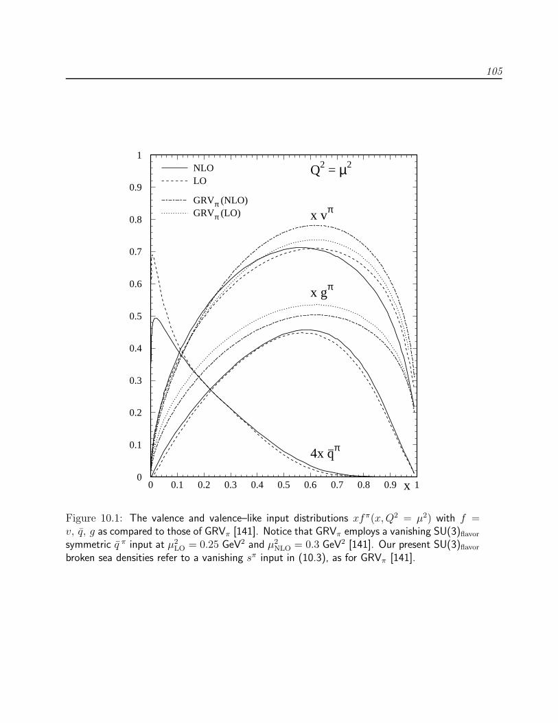
105

NLOLO

GRVπ (NLO)GRVπ (LO)

Q2 = µ2

x

x vπ

x gπ

4x q_π

0

0.1

0.2

0.3

0.4

0.5

0.6

0.7

0.8

0.9

1

0 0.1 0.2 0.3 0.4 0.5 0.6 0.7 0.8 0.9 1

Figure 10.1: The valence and valence–like input distributions xfπ(x,Q2 = µ2) with f =v, q, g as compared to those of GRVπ [141]. Notice that GRVπ employs a vanishing SU(3)flavorsymmetric q π input at µ2

LO = 0.25 GeV2 and µ2NLO = 0.3 GeV2 [141]. Our present SU(3)flavor

broken sea densities refer to a vanishing sπ input in (10.3), as for GRVπ [141].

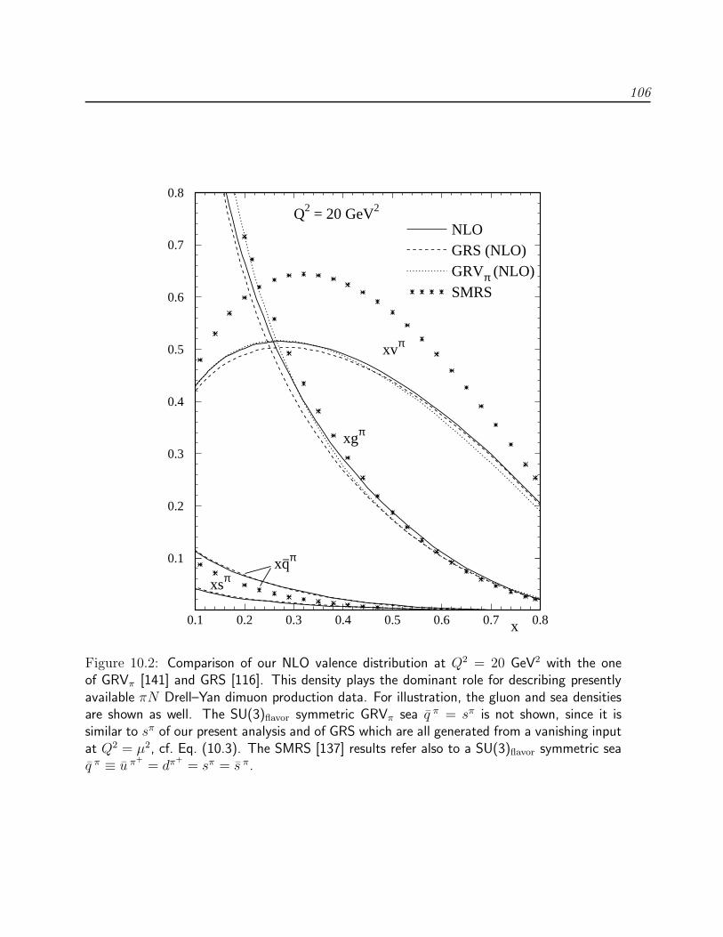
106

Q2 = 20 GeV2

NLOGRS (NLO)GRVπ (NLO)SMRS

x

xvπ

xgπ

xq_π

xsπ

0.1

0.2

0.3

0.4

0.5

0.6

0.7

0.8

0.1 0.2 0.3 0.4 0.5 0.6 0.7 0.8

Figure 10.2: Comparison of our NLO valence distribution at Q2 = 20 GeV2 with the oneof GRVπ [141] and GRS [116]. This density plays the dominant role for describing presentlyavailable πN Drell–Yan dimuon production data. For illustration, the gluon and sea densitiesare shown as well. The SU(3)flavor symmetric GRVπ sea q π = sπ is not shown, since it issimilar to sπ of our present analysis and of GRS which are all generated from a vanishing inputat Q2 = µ2, cf. Eq. (10.3). The SMRS [137] results refer also to a SU(3)flavor symmetric seaq π ≡ u π+

= dπ+= sπ = s π.

107

updated input in Fig. 10.1 is, as expected, rather similar to the one of [116]. In both cases,

however, the valence and gluon distributions become practically indistinguishable from

our present updated ones at scales relevant for present Drell–Yan dimuon and direct–γ

production data, Q2 ≡ M2µ+µ− ≃ 20 GeV2, as illustrated in Fig. 10.2. Therefore our

present updated pionic distributions give an equally good description of all available πN

Drell–Yan data as the ones shown in [116]. Notice that the different gluon distributions

presented in Fig. 10.2 can not be discriminated by present direct–photon production data

[138–140] due to the uncertainty of the theoretically calculated cross section arising from

variations of the chosen factorization scale and from possible intrinsic kT contributions,

cf. for example L. Apanasevich et al. [138–140].

For completeness let us mention that our basic predictions (10.5) for the valence–like

gluon and sea densities at Q2 = µ2, as shown in Fig. 10.1, can be simply parametrized in

Bjorken–x space : in LO at Q2 = µ2LO = 0.26 GeV2

x gπ(x, µ2LO) = 7.326 x1.433(1− 1.919

√x+ 1.524 x)(1− x)1.326

x q π(x, µ2LO) = 0.522 x0.160(1− 3.243

√x+ 5.206 x)(1− x)5.20 , (10.12)

whereas in NLO at Q2 = µ2NLO = 0.40 GeV2 we get

x gπ(x, µ2NLO) = 5.90 x1.270(1− 2.074

√x + 1.824 x)(1− x)1.290

x q π(x, µ2NLO) = 0.417 x0.207(1− 2.466

√x + 3.855 x)(1− x)4.454. (10.13)

Finally, Fig. 10.3 shows our resulting predictions for x gπ(x,Q2) and x q π(x,Q2) as

compared to the former GRVπ results [141]. The GRVπ results for x q π are significantly

steeper and softer for x >∼ 0.01 due to the vanishing SU(3)flavor symmetric (light) sea input

x q π(x, µ2) = 0, in contrast to our present approach [116] based on a more realistic finite

light sea input in Eq. (10.5). The valence–like gluon and sea inputs at Q2 = µ2, which

become (vanishingly) small at x < 10−2, are also shown in Fig. 10.3. This illustrates again

the purely dynamical origin of the small–x structure of gluon and sea quark densities at

Q2 > µ2. Our predictions for sπ = s π, as evolved from the vanishing input in Eq. (10.3),

are not shown in the figure since they practically coincide with q π(x,Q2) of GRVπ shown in

Fig. 10.3 which also results from a vanishing input [141]. Simple analytic parametrizations

of our LO and NLO predictions for fπ(x,Q2) are given in Appendix D.

To conclude let us recall that an improvement of fπ(x,Q2) is particularly important

in view of its central role in the construction of the photon structure function and the

108

x gπ(x,Q2)

x

100 = Q2 (GeV2)

20

5

(x 10)

(x 0.1)

µ2

(0.1 x)

x q_π(x,Q2) NLO

LO

GRVπ (NLO)GRVπ (LO)

100

20

5

(x 10)

(x 0.1)µ2

(x 0.1)

x10

-2

10-1

1

10

10 2

10 3

10-4

10-3

10-2

10-1

110

-3

10-2

10-1

1

10

10 2

10-4

10-3

10-2

10-1

1

Figure 10.3: The small–x predictions of our radiatively generated pionic gluon and sea–quarkdistributions in LO and NLO at various fixed values of Q2 as compared to those of GRVπ

[141]. The valence–like inputs, according to Eq. (10.5) as presented in Fig. 10.1, are shownfor illustration by the lowest curves referring to µ2. The predictions for the strange sea densitysπ = s π are similar to the GRVπ results for q π. The results are multiplied by the numbersindicated in brackets.

photonic parton distributions [96, 97, 112–114, 149]. Furthermore, recent (large rapidity

gap) measurements of leading proton and neutron production in deep inelastic scattering

at HERA [150] allow, under certain (diffractive) model assumptions, to constrain and test

the pion structure functions for the first time at far smaller vales of x (down to about

10−3) than those attained from fixed target πN experiments.

Chapter 11

Radiatively Generated PartonDistributions of Real and VirtualPhotons

Having presented the general theoretical framework in Chapter 9 we now turn to an anal-

ysis of the partonic content of (virtual) photons within the phenomenologically successful

framework of the radiative parton model [26, 41, 57, 92, 93]. This analysis follows Ref. [6].

The results in Sec. 11.3 have been taken from [7].

11.1 Introduction

Modern theoretical QCD studies [96, 112, 113, 149, 151] of the parton distributions of real,

i.e. on–shell, photons f γ(x,Q2), f = q, q, g, agree surprisingly well with measurements

of the (anti–)quark and gluon contents of the resolved real photons as obtained from

e+e− and ep reactions at collider energies (for recent reviews, see [89, 114, 152]). For

clarity let us denote the resolved real target photon with virtuality P 2 ≡ −p2 ≃ 0 by

γ ≡ γ(P 2 ≃ 0) which is probed by the virtual probe photon γ∗(Q2), Q2 ≡ −q2, via the

subprocess γ∗(Q2)γ → X as in e+e− → e+e−X . Here, p denotes the four–momentum of

the photon emitted from, say, an electron in an e+e− or ep collider. In the latter case it is

common to use Q2 instead of P 2 for denoting the photon’s virtuality, but we prefer P 2 for

the subprocess γ(P 2)p → X according to the original notation used in e+e− annihilations.

(Thus the factorization scale in f γ(P 2)(x,Q2) refers now to some properly chosen scale of

the produced hadronic system X , e.g. Q ∼ pjetT in high–pT jet events, etc.).

11.1 Introduction 110

In general one expects [97, 104, 111, 125–127, 153–155] also a virtual photon γ(P 2 6= 0)

to possess a parton content f γ(P 2)(x,Q2). It is a major problem to formulate a consistent

set of boundary conditions which allow for a calculation of f γ(P 2)(x,Q2) also in the next–

to–leading order (NLO) of QCD as well as for a smooth transition to P 2 = 0, i.e. to the

parton distributions of a real photon (see Refs. [97, 111, 156] for a detailed discussion).

Indeed, experimental studies of the transition of the deep inelastic (di–)jet cross section

from the real photon to the virtual photon region at HERA point to the existence of a

nonvanishing, though suppressed, parton content for virtual photons [157–161]. These

measurements have triggered various analyses of the dependence of the ep jet production

cross section on the virtuality of the exchanged photon [162, 163] and experimental tests of

such predictions will elucidate the so far unanswered question as to when a deep inelastic

scattering (DIS) ep process is eventually dominated by the usual ‘direct’ γ∗ ≡ γ(P 2)

induced cross sections, not contaminated by the so far poorly known resolved virtual

photon contributions. More recently, NLO calculations of the (di–)jet rate in ep (and

eγ) scattering, which properly include the contributions of resolved virtual photons, have

become available [164] and the resolved virtual photon contributions have already been

included in a Monte Carlo event generator [165] as well.

It is the main purpose of the present chapter to formulate a consistent set of boundary

conditions, utilizing valence–like input parton distributions at the universal target–mass

independent [41, 57, 93, 96, 112, 141] low resolution scale Q20 = µ2 ≃ 0.3 GeV2, which allow

for a calculation of f γ(P 2)(x,Q2) also in NLO–QCD as well as for a smooth transition to

the parton distributions of a real photon, P 2 = 0. We shall furthermore employ the pionic

parton distributions of Chapter 10, fπ(x,Q2), which are required for describing, via vector

meson dominance (VMD), the hadronic components of the photon. It should be recalled

that the pionic gluon and sea densities, gπ(x,Q2) and q π(x,Q2), have been uniquely

derived from the experimentally rather well known pionic valence density vπ(x,Q2) and

the (recently updated [26] dynamical) parton distributions f(x,Q2) of the proton. Thus

we arrive at essentially parameter–free predictions for f γ(P 2)(x,Q2) which are furthermore

in good agreement with all present measurements of the structure function of real photons,

F γ2 (x,Q

2).

Sec. 11.2 is devoted to an analysis of the parton distributions and structure functions

of real photons and the resulting predictions are compared with recent experiments. In

Sec. 11.3 we compare our unique small–x predictions –characteristic for the radiative

11.2 The Parton Content of Real Photons 111

parton model– with very recent small–x measurements of the photon structure function

F γ2 (x,Q

2) by the LEP–OPAL collaboration. Sec. 11.4 contains the formulation of our

model for the parton distributions of virtual photons, together with some quantitative

predictions for structure functions as well as a comparison with very recent data extracted

from DIS dijet events. Our conclusions are drawn in Sec. 11.5. In App. D we present simple

analytic parametrizations of our LO and NLO predictions for the parton distributions of

real and virtual photons.

11.2 The Parton Content of Real Photons

11.2.1 Boundary Conditions

The pionic parton distributions presented in the previous chapter will now be utilized

to construct LO and NLO input distributions for the real photon via a vector meson

dominance ansatz at the low resolution scale Q20 = µ2 ≃ 0.3 GeV2.

In NLO the nonperturbative hadronic VMD input f γ(x,Q20) refers to the partons in

the DISγ scheme which guarantees the perturbative stability of the resulting F γ2 (x,Q

2)

provided this input is given by the NLO fπ(x,Q20) of Chap. 10, while the corresponding

input in LO is given via VMD by the LO fπ(x,Q20) of Chap. 10. We shall assume that

the input resolution scale Q20 = µ2 ≃ 0.3 GeV2 for the valence–like parton structure is

universal, i.e. independent of the mass of the considered targets p, π, γ, etc. [41, 57, 93,

96, 112, 116, 141].

The hadronic VMD ansatz for f γ(x, µ2) is based on a coherent superposition of vector

mesons [97]

|γ〉µ2, had ≃ e

fρ|ρ〉µ2 +

e

f ω

|ω〉µ2 (11.1)

where the φ–meson contribution is considered to be strongly suppressed at µ2 ≪ m2φ. As

usual, we identify the parton distribution functions in the parton model with matrix ele-

ments of local twist–2 operators within the operator product expansion (OPE) formalism

and we obtain using (11.1)

f γ(µ2) = f γhad(µ

2) = 〈γ|Of |γ〉µ2,had

=e2

f 2ρ

〈ρ|Of |ρ〉µ2 +e2

fρfω(〈ρ|Of |ω〉µ2 + 〈ω|Of |ρ〉µ2) +

e2

f 2ω

〈ω|Of |ω〉µ2

11.2 The Parton Content of Real Photons 112

with f = u, d, s, g. Assuming, within the OPE,

〈ρ|Oq|ρ〉µ2 = 〈ω|Oq|ω〉µ2 = 〈π0|Oq|π0〉µ2 , 〈ρ|Oq|ω〉µ2 = 2 I3q e−iθ〈π0|Oq|π0〉µ2

〈ρ|Og|ρ〉µ2 = 〈ω|Og|ω〉µ2 = 〈π0|Og|π0〉µ2 , 〈ρ|Og|ω〉 = 0

where the last equation holds due to isospin conservation, one obtains

(u+ u)γ(x, µ2) = α(g2ρ + g2ω + 2 gρgω cos θ)(u+ u)π0

(x, µ2)

(d+ d)γ(x, µ2) = α(g2ρ + g2ω − 2 gρgω cos θ)(d+ d)π0

(x, µ2)

(s+ s)γ(x, µ2) = α(g2ρ + g2ω) (s+ s)π0

(x, µ2) = 0

gγ(x, µ2) = α(g2ρ + g2ω) gπ0

(x, µ2). (11.2)

Here Oq,g refer to the leading twist–2 quark and gluon operators and g2V ≡ 4π/f 2V with

g2ρ = 0.50 , g2ω = 0.043 , (11.3)

i.e. f 2ρ/4π = 2.0 and f 2

ω/4π = 23.26, as obtained from a zero–width calculation of the

relevant leptonic widths Γ(V → ℓ+ℓ−) = α2mV g2V /3 presented in [166]. The omission of a

finite–width correction for g2ρ is due to the central role [166] of the precise results in [167]

which do not require such a correction in contrast to the situation for the less precise

resonance analysis at e+e− colliders [85, 168, 169].

For the a priori unknown coherence factor (fit parameter) cos θ in Eq. (11.2) we take

cos θ = 1, i.e. we favor a superposition of u and d quarks which maximally enhances

the contributions of the up–quarks to F γ2 in Eq. (9.1). This favored value for cos θ is

also supported by fitting cos θ in (11.2) to all presently available data on F γ2 (x,Q

2), to

be discussed below, which always resulted in cos θ ≃ 1 in LO as well as NLO. This is

also in agreement with the LO results obtained in Ref. [97]. The LO and NLO input

distributions fπ(x, µ2) of the pion in (11.2) are taken from the analysis in the previous

chapter which correspond to [5, 26] µ2LO = 0.26 GeV2 and µ2

NLO = 0.40 GeV2 in LO and

NLO, respectively. Since by now all free input quantities have been fixed in Eq. (11.2),

we arrive at rather unique parameter–free predictions for f γ(x,Q2) and F γ2 (x,Q

2).

The calculation of f γ(x,Q2) at Q2 > µ2 follows from the well known inhomogeneous

renormalization group (RG) evolution equations in LO and NLO which we solve, as

usual, analytically for the n–th Mellin moment of f γ(x,Q2), followed by a straightforward

Mellin–inversion to Bjorken–x space as described in detail in Chapter 9. The general

11.2 The Parton Content of Real Photons 113

structure of these solutions is

f γ(x,Q2) = f γpl(x,Q

2) + f γhad(x,Q

2) . (11.4)

Here f γpl denotes the perturbative ‘pointlike’ solution which vanishes at Q2 = µ2 and is

driven by the pointlike photon splitting functions k(0,1)q,g (x) appearing in the inhomogeneous

evolution equations, while f γhad depends on the hadronic input f γ(x, µ2) in Eq. (11.2) and

evolves according to the standard homogeneous evolution equations.

The prescription for the VMD ansatz in Eq. (11.2) at the input scale µ2, together with

cos θ = 1 as discussed above, yields a simple expression for the general Q2–dependence of

f γ(x,Q2):

f γ(x,Q2) = f γpl(x,Q

2) + α

[G2

f fπ(x,Q2) + δf

1

2(G2

u −G2d) s

π(x,Q2)

](11.5)

with δu = −1, δd = +1 and δs = δg = 0, and where the index π obviously refers to π0 and

G2u = (gρ + gω)

2 ≃ 0.836

G2d = (gρ − gω)

2 ≃ 0.250

G2s = G2

g = g2ρ + g2ω = 0.543 . (11.6)

Simple analytic LO and NLO(DISγ) parametrizations for the pointlike piece f γpl(x,Q

2)

are given in App. D.2, whereas the ones for fπ(x,Q2) can be found in App. D.1.

11.2.2 Quantitative Results

Having outlined the theoretical basis for our photonic parton distributions, we now turn

to the quantitative results. First we apply our parameter–free predictions for f γ(x,Q2)

to the structure function of real photons which, according to Eq. (9.1), is finally given by

1

xF γ2 (x,Q

2) = 2∑

q=u,d,s

e2q

{qγ(x,Q2) +

αs(Q2)

2π[Cq,2 ⊗ qγ + Cg,2 ⊗ gγ]

}

+1

xF γ2,c(x,Q

2) +1

xF gγ

2,c(x,Q2) (11.7)

where f γ(x,Q2) refers to the DISγ factorization scheme defined in (9.9) and the charm

contributions F γ2,c and F gγ

2,c are given by Eqs. (9.13) and (9.14), respectively.

11.2 The Parton Content of Real Photons 114

0

0.2

0.4

0

0.2

0.4

0

0.2

0.4

0.6

10-3

10-2

10-1

10-3

10-2

10-1

10-3

10-2

10-1

OPAL Q2 (GeV2) = 1.86

F2 γ /α NLO

LOGRVγ (NLO)GRVγ (LO)

L3 set1 1.9L3 set2 1.9

PLUTO 2.4 OPAL 3.76

PLUTO 4.3 L3 set1 5.0

L3 set2 5.0

TOPAZ 5.1 PLUTO 5.3

DELPHIprl 6.5AMY 6.8

OPAL 7.5OPAL2 9.0

ALEPHprl 8.9PLUTO 9.2

DELPHI 12.0DELPHIprl 13.0

x10-3

10-2

10-1

0

0.25

0.5

0.75

1

0

0.5

1

0

0.5

1

1.5

0.5 1 0.5 1 0.5 1

OPAL 14.7OPAL2 14.5

TOPAZ 16 ALEPHprl 19.1DELPHIprl 22.0

TASSO 23JADE 24

OPAL2 30 PLUTO 45 OPAL2 59 AMY 73TOPAZ 80

JADE 100 OPAL 135 ALEPHprl 279 AMY 390

x0.5 1

Figure 11.1: Comparison of our radiatively generated LO and NLO(DISγ) predictions forF γ2 (x,Q

2), based on the valence–like parameter–free VMD input in Eq. (11.2), with the dataof Ref. [170–179]. For our comparison the GRVγ [96, 112] results are shown as well. In bothcases, the charm contribution has been added, in the relevant kinematic region W ≥ 2mc,according to Eqs. (9.13) and (9.14).

11.2 The Parton Content of Real Photons 115

0

0.1

0.2

0.3

0.4

0.5

0

0.1

0.2

0.3

0.4

0

0.2

0.4

0.6

0.8

0 0.2 0.4 0.6 0.8 1

x uγ(x,Q2) /α LO

Q2 = 10 GeV2 Q2 = 10 GeV2x uγ(x,Q2) /α NLO

totalhad

GRVγ

SaS 1DSaS 2D

Q2 = 10 GeV2

x dγ(x,Q2) /α LO

totalhad

GRVγ

AFG

Q2 = 10 GeV2

x dγ(x,Q2) /α NLO

x

Q2 = 10 GeV2

x gγ(x,Q2) /α LO

Q2 = 10 GeV2

x

x gγ(x,Q2) /α NLO

0 0.2 0.4 0.6 0.8 1

Figure 11.2: Comparison of our predicted LO and NLO(DISγ) distributions uγ = u γ , dγ = d γ

and gγ at Q2 = 10 GeV2 with the LO/NLO GRVγ densities [96, 112], the LO SaS 1D and 2D[97] and the NLO AFG [113] distributions. The ‘hadronic’ (pionic) components of our totalLO and NLO results in Eq. (11.4) are displayed by the dashed curves.

11.2 The Parton Content of Real Photons 116

In Fig. 11.1 we compare our LO and NLO predictions with all available1 relevant data

[170–179] for F γ2 of the real photon. Our present new NLO results are rather similar to

the ones of AFG [113], but differ from the previous (GRVγ) predictions [96, 112] which

are steeper in the small–x region, as shown in Fig. 11.1, because the dominant hadronic

(pionic) sea density q π(x,Q2) is steeper since it has been generated purely dynamically

from a vanishing input at Q2 = µ2 [96, 112, 141]. Similarly the SaS 1D [97] expectations,

for example, fall systematically below the data in the small to medium Q2 region around

Q2 ≃ 5 GeV2, partly due to a somewhat different treatment of the hadronic coherent

VMD input as compared to our results in Eqs. (11.2), (11.5), and (11.6).

The relevant LO and NLO photonic parton densities are compared in Fig. 11.2 at Q2 =

10 GeV2. For illustration we also show the purely ‘hadronic’ component (homogeneous

solution) in (11.4) of f γ which demonstrates the dominance of the ‘pointlike’ component

(inhomogeneous solution) in (11.4) for uγ and dγ in the large–x region, x > 0.1 .

In Fig. 11.3 we show our predictions for xuγ(x,Q2) and xgγ(x,Q2). The parton dis-

tributions of the photon behave, in contrast to the ones of a hadron, very differently in

the limits of large and small x. In the former case, the purely perturbative pointlike

part in (11.4) dominates for x >∼ 0.1, especially for the quark distributions. On the other

hand, this uniquely calculable contribution amounts at most to about 20% at very small

x where the hadronic VMD component in (11.4) dominates, giving rise to a very sim-

ilar increase for x → 0 as observed in the proton case. In Fig. 11.3 we also show our

valence–like inputs at Q2 = µ2LO,NLO which become (vanishingly) small at x < 10−2. This

illustrates the purely dynamical origin of the small–x increase at Q2 > µ2. Also note-

worthy is the perturbative LO/NLO stability of uγ(x,Q2) which is almost as good as the

one required for a physical quantity like F γ2 (x,Q

2) in Fig. 11.1. The situation is, as usual

[26, 41, 57, 93, 96, 112], different for gγ(x,Q2). Nevertheless, despite the sizable difference

between the LO and NLO gluon distributions in Fig. 11.3 in the small–x region, the di-

rectly measurable F γ2 and the gluon–dominated heavy quark contribution in Eq. (9.14)

shows a remarkable perturbative stability [26].

Next, we compare in Fig. 11.4 our predictions for xgγ(x,Q2) at Q2 ≡ (pjetT )2 = 75 GeV2

with recent HERA (H1) measurements [180, 181]. Our somewhat flatter results for xgγ

in the small–x region, as compared to the older GRVγ expectations [96, 112], is caused by

the recently favored flatter gluon distribution in the proton [26] which determines gγ via

1January 1999

11.2 The Parton Content of Real Photons 117

x uγ(x,Q2) /α

x

100 = Q2 (GeV2)

20

5

µ2

(x 10)

(x 0.1)

(0.1 x)

NLONLOhad

LO

GRVγ (NLO)

x

x gγ(x,Q2) /α100 = Q2 (GeV2)

(x 10)

20

5

(x 0.1)

µ2

(x 0.1)

10-2

10-1

1

10

10 2

10-4

10-3

10-2

10-1

110

-3

10-2

10-1

1

10

10 2

10 3

10-4

10-3

10-2

10-1

1

Figure 11.3: Detailed small–x (as well as large–x) behavior and predictions of our radiativelygenerated uγ = u γ and gγ distributions in LO and NLO(DISγ) at fixed values of Q2. Thedashed–dotted curves show the hadronic NLO contribution f γ

had to f γ = f γpl + f γ

had in Eq.(11.4). The valence–like inputs at Q2 = µ2

LO,NLO, according to Eq. (11.2), are shown bythe lowest curves referring to µ2. For comparison we show the steeper NLO GRVγ [96, 112]expectations as well. The results have been multiplied by the number indicated in brackets.

gπ [5], cf. Eq. (11.2), at small x.

Finally it is interesting to consider the total momenta carried by the photonic partons,

Mγ2 (Q

2) ≡∑

f=q,q,g

∫ 1

0

x f γ(x,Q2) dx . (11.8)

Inspired by the ideas and suggestions put forward in Refs. [97, 128], it has been conjectured

recently [129] that this leading twist–2 quantity Mγ2 should satisfy, in LO-QCD,

Mγ2 (Q

2) ≃ Πh(Q2) (11.9)

where the well known dispersion relation relates the hadronic part of the photon’s vacuum

polarization

Πh(Q2) =

Q2

4π2α

∫ ∞

4m2π

σh(s)

s+Q2ds (11.10)

11.3 The Photon Structure Function at Small–x 118

x gγ(x,Q2=75 GeV2)/α H1 dijet events

H1 high pT track events

NLOLO

GRVγ (NLO)GRVγ (LO)

SaS1D (LO)

x-1

0

1

2

3

4

5

6

10-2

10-1

1

Figure 11.4: Comparison of our LO and NLO predictions for xgγ at Q2 ≡ 〈(pjetT )2〉 = 75GeV2 with HERA(H1) measurements [180, 181]. The GRVγ and SaS expectations are takenfrom Refs. [96, 112] and [97], respectively.

to σh ≡ σ(e+e− → hadrons). It should be noted that Πh(Q2), being an experimental

quantity, includes, besides the usual twist–2 term, all possible nonperturbative higher–

twist contributions. The ‘consistency’ relation (11.9) is, however, expected to hold already

atQ2 >∼ 2 to 4 GeV2 to within, say, 20 to 30% where the twist–2 component in Πh(Q2) may

become dominant, as possibly indicated by DIS ep processes. Indeed, our LO results imply

Mγ2 (2 GeV2)/α ≃ 0.976 and Mγ

2 (4 GeV2)/α ≃ 1.123 which compares favorably with [182]

Πh(2 GeV2)/α = 0.694± 0.028 and Πh(4 GeV2)/α = 0.894± 0.036, respectively.

11.3 The Photon Structure Function at Small–x

Recently the OPAL collaboration [98] at the CERN–LEP collider has extended the mea-

surements of the photon structure function F γ2 (x,Q

2) into the small–x region down to

x ≃ 10−3, probing lower values of x than ever before. The observed rise of F γ2 towards

low values of x, x < 0.1, is in agreement with general QCD renormalization group im-

proved expectations. It has, however, been noted that the rising small–x data at lower

11.3 The Photon Structure Function at Small–x 119

scales Q2 ≃ 2 − 4 GeV2 lie above the original QCD expectations anticipated almost a

decade ago [96, 97].

In the following we will demonstrate that our updated parameter–freeQCD predictions

for F γ2 (x,Q

2) [6], discussed in Sec. 11.2, are in general also consistent with the OPAL

small–x measurements at all presently accessible values of Q2.

Before presenting our results it is instructive to recapitulate briefly the main differences

between the original GRVγ [96] approach to the photonic parton distributions and our

parameter–free predictions of Sec. 11.2. In the latter approach a coherent superposition of

vector mesons has been employed, which maximally enhances the u–quark contributions

to F γ2 , for determining the hadronic parton input f γ

had(x,Q20) at a GRV–like [26] input

scale Q20 ≡ µ2

LO = 0.26 GeV2 and Q20 ≡ µ2

NLO = 0.40 GeV2 for calculating the (anti)quark

and gluon distributions f γ(x,Q2) of a real photon in leading order (LO) and next–to–

LO (NLO) of QCD. Furthermore, in order to remove the ambiguity of the hadronic

light quark sea and gluon input distributions of the photon (being related to the ones of

the pion, fπ(x,Q20), via vector meson dominance), inherent to the older GRVγ [96] and

SaS [97] parametrizations, predictions [5, 116] for q π(x,Q2) and gπ(x,Q2), cf. Chapter

10, have been used in our present approach which follow from constituent quark model

constraints [94, 95]. These latter constraints allow to express q π and gπ entirely in terms

of the experimentally known pionic valence density and the rather well known quark–

sea and gluon distributions of the nucleon, using most recent updated valence–like input

parton densities of the nucleon. Since more recent DIS small–x measurements at HERA

imply somewhat less steep sea and gluon distributions of the proton [26], the structure

functions of the photon will therefore also rise less steeply in x than the previous GRVγ

[96] ones as was already discussed in the previous section and as will be seen in the figures

shown below. In this way one arrives at truly parameter–free predictions for the structure

functions and parton distributions of the photon.

In Figs. 11.5 and 11.6 we compare our predictions of Section 11.2, denoted by GRSc

[6] and the older GRVγ results [96] with the recent small–x OPAL measurements [98] and,

for completeness, some relevant L3 data [179] are shown as well. Our parameter–free LO

and NLO expectations are confirmed by the small–x OPAL data2 at all (small and large)

experimentally accessible scales Q2. This is in contrast to the GRVγ and SaS results

2Note that the new OPAL data [98] at Q2 = 1.9 and 3.7 GeV2 supersede the older OPAL data shownin Fig. 11.1 at Q2 = 1.86 and 3.76 GeV2, see [98].

11.3 The Photon Structure Function at Small–x 120

which at LO are somewhat below the data at small Q2 in Fig. 11.5 and seem to increase

too strongly at small x in NLO, in particular at larger values of Q2 as shown in Fig.

11.6. The main reason for this latter stronger and steeper x–dependence in LO and NLO

derives from the assumed vanishing (pionic) quark–sea input at Q20 = µ2

LO,NLO for the

anti(quark) distributions of the photon as well as from relating the hadronic gluon input

of the photon directly to its (pionic) valence distribution [96, 141]. This is in contrast to

the more realistic (input) boundary conditions employed here.

Clearly these small–x measurements imply that the photon must contain [98] a dom-

inant hadron–like component at low x, since the simple direct ‘box’ cross section (based

on the subprocess γ∗(Q2)γ → qq ) yields F γ2,box → 0 as x → 0, in contrast to the data

for x < 0.1 in Figs. 11.5 and 11.6. The QCD RG–improved parton distributions of

the photon are thus essential for understanding the data on F γ2 (x,Q

2), with its domi-

nant contributions deriving from qγ(x,Q2) = q γ(x,Q2). It would be also interesting and

important to extend present measurements [89, 90, 180, 181] of the gluon distribution of

the photon, gγ(x,Q2), below the presently measured region 0.1 <∼ x < 1 where similarly

gγ(x < 0.1, Q2) is expected to be also somewhat flatter, see Fig. 11.4, in the small–x

region than previously anticipated [96].

11.3 The Photon Structure Function at Small–x 121

0

0.1

0.2

0.3

0.4

0.5

0.6OPAL (1.9)

L3 set1 (1.9)

L3 set2 (1.9)

Q2=1.9 GeV2

F 2 γ (x,Q

2 ) /α

GRSc (NLO)

GRSc (LO)

GRVγ (NLO)

GRVγ (LO)

SaS 1D

OPAL (3.7)

Q2=3.7 GeV2

x0

0.1

0.2

0.3

0.4

0.5

10-3

10-2

10-1

Figure 11.5: Comparison of our parameter–free predictions from Sec. 11.2 denoted by GRSc[6], the previous GRVγ [96] and SaS [97] results for F γ

2 (x,Q2) with the recent OPAL

(1.9 GeV2) small–x measurements [98] at two fixed lower scales Q2. Some relevant L3data [179] are displayed as well.

11.3 The Photon Structure Function at Small–x 122

0

0.1

0.2

0.3

0.4

0.5

0.6

0.7OPAL (10.7) GRSc (NLO)

GRSc (LO)

GRVγ (NLO)

GRVγ (LO)

SaS 1D

Q2=10.7 GeV2

F 2 γ (x,Q

2 ) /α

OPAL (17.5,17.8)

Q2=17.8 GeV2

x

0

0.2

0.4

0.6

0.8

1

10-3

10-2

10-1

Figure 11.6: As in Fig. 11.5 but at two fixed scales Q2. The recent OPAL small–x data aretaken from Ref. [98].

11.4 The Parton Content of Virtual Photons 123

11.4 The Parton Content of Virtual Photons

Next we turn to the somewhat more speculative concept and models of ‘resolved’ virtual

photons (P 2 6= 0). As motivated in Chap. 9 the dependence on the target virtuality

P 2 will be entirely taken care of by the boundary conditions whereas the partons will

be treated as if they were on–shell. Of course, this is quite familiar for the quarks and

gluons, however, the latter rule also refers to the photon–parton Γγ(P 2)(x,Q2) in the target

photon, i.e., the ’direct’ subprocesses, e.g., γ⋆(Q2)Γγ(P 2) → qq have to be calculated with

P 2 = 0 (cf. rule (ii) in [6]). Thus we can implement the same DISγ factorization scheme

as for real photons in Eq. (9.9), and the structure function Fγ(P 2)2 (x,Q2) of a transverse

virtual target photon becomes formally very similar to Eq. (11.7):

1

xF

γ(P 2)2 (x,Q2) = 2

∑

q=u,d,s

e2q

{qγ(P

2)(x,Q2) +αs(Q

2)

2π

[Cq,2 ⊗ qγ(P

2) + Cg,2 ⊗ gγ(P2)]}

+1

xF γ2,c(x,Q

2) +1

xF gγ(P

2)

2,c (x,Q2) (11.11)

with Cq,2(x), Cg,2(x) given in (9.5). The ‘direct’ heavy (charm) quark contribution is given

by Eq. (9.13) as for real photons and the ‘resolved’ charm contribution F gγ(P2)

2,c is as in

Eq. (9.14) with the gluon distribution gγ(z, µ2F ) → gγ(P

2)(z, µ2F ).

It is physically compelling to expect a smooth behavior of the observable structure

function in Eq. (11.11) with respect to P 2. Especially, in the real photon limit Eq. (11.7)

has to be recovered imposing the condition f γ(P 2)(x,Q2) → f γ(x,Q2) as P 2 → 0 for the

parton distributions. Note that this requirement is automatically satisfied as soon as it

has been implemented at the input scale Q20 since the PDFs are governed by the same

evolution equations which is a consequence of our unified approach.

11.4.1 Boundary Conditions

The above smoothness requirements are fulfilled by the following boundary conditions for

f γ(P 2), cf. Eq. (11.5),

f γ(P 2)(x,Q2 = P 2) = fγ(P 2)had (x, P 2) = η(P 2)f γ

had(x, P2) (11.12)

in LO as well as in NLO. Here P 2 = max (P 2, µ2) as dictated by continuity in P 2 [111] and

η(P 2) = (1+P 2/m2ρ)

−2 is a dipole suppression factor with m2ρ = 0.59 GeV2. The scale P 2

11.4 The Parton Content of Virtual Photons 124

is dictated not only by the above mentioned continuity requirement, but also by the fact

that the hadronic component of f γ(P 2)(x,Q2) is probed at the scale Q2 = P 2 [97, 111, 154]

where the pointlike component vanishes by definition. The boundary condition in Eq.

(11.12) guarantees, as should be evident, a far better perturbative stability as compared

to the situation in [111] where the NLO input differed drastically from its LO counterpart

(cf. Eq. (8) in Ref. [111]).

The evolution to Q2 > P 2 is now analogous to the case of real photons in the previous

section and the general solution for the resulting parton distributions is similar to the one

in Eq. (11.4) and Eq. (11.5),

f γ(P 2)(x,Q2) = fγ(P 2)pl (x,Q2) + f

γ(P 2)had (x,Q2) (11.13)

= fγ(P 2)pl (x,Q2) + η(P 2)α

[G2

f fπ(x,Q2) + δf

1

2(G2

u −G2d) s

π(x,Q2)

]

with δf as in Eq. (11.5) and where fγ(P 2)had refers again to the solution of the homogeneous

RG evolution equations, being driven by the hadronic input in (11.12), which is explicitly

given by Eq. (9.25). Its parametrization is fixed by the available parametrization for

fπ(x,Q2) in App. D.1. The inhomogeneous ‘pointlike’ solution in (11.13) is explicitly

given by Eq. (9.24) where L = αs(Q2)/αs(P

2). A parametrization of fγ(P 2)pl (x,Q2) in LO

is thus easily obtained from the one for the real photon f γpl(x,Q

2) in (11.5) in terms of

ln L−1 = ln [αs(µ2)/αs(Q

2)], where now αs(µ2) has simply to be replaced by αs(P

2) as

described in detail in App. D.2. Furthermore, since our NLO predictions for f γ(P 2)(x,Q2)

turn out to be rather similar to the LO ones, as will be shown below, the simple analytic

LO parametrizations for f γ(P 2)(x,Q2) can be used for NLO calculations as well. This is

certainly sufficiently accurate and reliable in view of additional model ambiguities inherent

in the parton distributions of virtual photons.

It should be emphasized that the RG resummed results in (11.13) are relevant when-

ever P 2 ≪ Q2, typically [111, 162] P 2 ≃ 110

Q2, so as to suppress power–like (possibly

higher twist) terms (P 2/Q2)n which would spoil the dominance of the resummed loga-

rithmic contributions. For P 2 approaching Q2, the e+e− → e+e−X reaction, for example,

should be simply described by the full fixed order box γ⋆(Q2)γ⋆(P 2) → qq keeping all

(P 2/Q2)n terms (cf. Chap. 8). A calculation of the full perturbative O(αs) corrections

to this virtual box [108] will offer the possibility to determine reliably at what values of

P 2 (and possibly x) this O(αs) corrected virtual box becomes the more appropriate and

correct description. Similar remarks hold for a DIS process ep → eX , i.e. γ(P 2) p → X ,

11.4 The Parton Content of Virtual Photons 125

where O(αs) corrections to pointlike virtual γ(P 2)–parton subprocesses have to be ana-

lyzed in detail in order to decide at what P 2 these pointlike expressions become the more

appropriate description and the virtual photonic parton distributions (i.e., resummations)

become irrelevant.

Our unified approach implies that the ‘direct’ photon contribution to any process

whatsoever should always be calculated as if this photon is real apart from the fact that

its flux should be evaluated according to Eq. (7.37) with P 2 6= 0 [155, 162, 163]. This

differs from the somewhat inconsistent procedure adopted by the HERA–H1 collabora-

tion [157–161] where exact e q → e q g and e g → e q q matrix elements were used for

the direct photon contribution to the dijet cross section. As long as P 2 <∼ 110Q2, the

exact treatment of matrix elements, however, should not differ too much [164] from the

more appropriate treatment described above. To conclude let us stress that our unified

approach, as illustrated by the foregoing examples, is not a free option but a necessary

consistency condition for introducing the concept of the resolved parton content of the

virtual photon as an alternative to a non–resummed fixed order perturbative analysis at

P 2 6= 0. This consistency requirement is related to the fact that all the resolved con-

tributions due to f γ(P 2)(x,Q2) are calculated (evoluted) as if these partons are massless

[7 − 11] (i.e. employing photon splitting functions for real photons, etc.) in spite of the

fact that their actual virtuality is given by P 2 6= 0. Thus the direct photon contribution

should obviously be also treated accordingly.

11.4.2 Quantitative Results

Now we turn to our quantitative predictions and we first present in Fig. 11.7 detailed

predictions for Fγ(P 2)2 (x,Q2) for various virtualities P 2 and scales Q2. Since the ‘pointlike’

component in (11.13) is uniquely calculable perturbatively, a detailed measurement of

the x and P 2 dependence at various fixed values of Q2, as shown in Fig. 11.7, would

shed light on the theoretically more speculative and far less understood nonperturbative

‘hadronic’ contribution in Eq. (11.13) and eventually establish the absolute perturbative

predictions. Our LO and NLO predictions in Fig. 11.7 show a remarkable perturbative

stability throughout the whole x–region shown, except perhaps for P 2 ≫ 1 GeV2 where

the perturbatively very stable [5, 116] ‘hadronic’ component in (11.13) becomes strongly

suppressed with respect to the ‘pointlike’ solution which is less stable in the small x region,

x < 10−2, as is evident from the right hand side of Fig. 11.7.

11.4 The Parton Content of Virtual Photons 126

10-3

10-2

10-1

1

P2 = 0

P2 = 0.35 GeV2

(x 0.1)

F 2 γ (P 2 )

(x,Q

2 ) /α

NLO

NLOhad

LO

GRS (NLO)

P2 = 1 GeV2

Q2 = 10 GeV2

x

10-3

10-2

10-1

10-4

10-3

10-2

10-1

1

10-3

10-2

10-1

1

P2 = 0

P2 = 1 GeV2

(x 0.1)

F 2 γ (P 2 )

(x,Q

2 ) /α

NLONLOhad

LO

GRS (NLO)

P2 = 10 GeV2

Q2 = 100 GeV2

x

10-4

10-3

10-2

10-1

10-4

10-3

10-2

10-1

1

Figure 11.7: LO and NLO predictions for the x dependence of the virtual photon structure

function Fγ(P 2)2 at Q2 = 10 and 100 GeV2 and various fixed values of P 2 ≪ Q2, neglecting

any heavy quark contribution. For comparison we also show the NLO Gluck–Reya–Stratmann(GRS) [111] results as well as the predictions for a real (P 2 = 0) photon. Notice that thedotted curve for P 2 = 0 referred to as GRS obviously coincides with the GRVγ result [96, 112].The results have been multiplied by the number indicated in brackets.

The individual LO and NLO parton distributions of the virtual photon at Q2 =

10 GeV2 are shown in Fig. 11.8 where they are compared with the ones of Gluck, Reya

and Stratmann (GRS) [111]. The LO SaS expectations [97] are compared with our LO

predictions in Fig. 11.9.

In Fig. 11.10 we show our predictions for xuγ(P 2)(x,Q2) and xgγ(P2)(x,Q2) with par-

ticular emphasis on the very small x region. For comparison we also show the results for a

real (P 2 = 0) photon. Plotting the ‘hadronic’ component in (11.13) separately in the up-

per two panels of Fig. 11.10 demonstrates that the perturbative ‘pointlike’ component in

(11.13) dominates for x > 10−2. In the lower two panels of Fig. 11.10, at P 2 = 5, 10 GeV2,

the hadronic part is nearly vanishing even at small x [η(P 2(GeV2) = 5, 10) = 0.01, 0.003].

Furthermore the expected perturbative stability of our present LO and NLO predictions

is fulfilled. This is in contrast to the GRS results which are unstable [111] throughout

the whole x–region for P 2 >∼ 1 GeV2, as illustrated in the lower half of Fig. 11.10 at

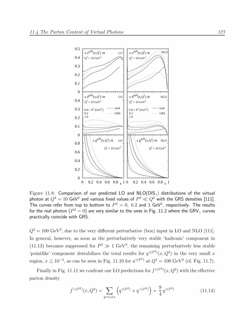
11.4 The Parton Content of Virtual Photons 127

0

0.1

0.2

0.3

0.4

0.5

0

0.1

0.2

0.3

0.4

0

0.2

0.4

0.6

0.8

0 0.2 0.4 0.6 0.8 1

x uγ(P 2)(x,Q2) /α LO

Q2 = 10 GeV2 Q2 = 10 GeV2

x uγ(P 2)(x,Q2) /α NLO

total

GRS

Q2 = 10 GeV2

0.0 = P2 (GeV2)0.21.0

x dγ(P 2)(x,Q2) /α LO

total

GRS

Q2 = 10 GeV2

0.0 = P2 (GeV2)0.21.0

x dγ(P 2)(x,Q2) /α NLO

x

Q2 = 10 GeV2

x gγ(P 2)(x,Q2) /α LO

Q2 = 10 GeV2

x

x gγ(P 2)(x,Q2) /α NLO

0 0.2 0.4 0.6 0.8 1

Figure 11.8: Comparison of our predicted LO and NLO(DISγ) distributions of the virtualphoton at Q2 = 10 GeV2 and various fixed values of P 2 ≪ Q2 with the GRS densities [111].The curves refer from top to bottom to P 2 = 0, 0.2 and 1 GeV2, respectively. The resultsfor the real photon (P 2 = 0) are very similar to the ones in Fig. 11.2 where the GRVγ curvespractically coincide with GRS.

Q2 = 100 GeV2, due to the very different perturbative (box) input in LO and NLO [111].

In general, however, as soon as the perturbatively very stable ‘hadronic’ component in

(11.13) becomes suppressed for P 2 ≫ 1 GeV2, the remaining perturbatively less stable

‘pointlike’ component destabilizes the total results for qγ(P2)(x,Q2) in the very small x

region, x <∼ 10−3, as can be seen in Fig. 11.10 for uγ(P 2) at Q2 = 100 GeV2 (cf. Fig. 11.7).

Finally in Fig. 11.11 we confront our LO predictions for f γ(P 2)(x,Q2) with the effective

parton density

f γ(P 2)(x,Q2) =∑

q=u,d,s

(qγ(P

2) + q γ(P 2))+

9

4gγ(P

2) (11.14)

11.4 The Parton Content of Virtual Photons 128

x uγ(P 2)(x,Q2) /α

Q2 = 10 GeV2

x

P2(GeV2) = 0

0.2

1.0

LOSaS 1DSaS 2D

x gγ(P 2)(x,Q2) /α

x

0 = P2(GeV2)

0.2

1.0

0

0.05

0.1

0.15

0.2

0.25

0.3

0.35

0.4

0.45

0.5

0 0.2 0.4 0.6 0.8 10

0.1

0.2

0.3

0.4

0.5

0.6

0.7

0.8

0.9

1

0 0.2 0.4 0.6 0.8 1

Figure 11.9: Our LO distributions as in Fig. 11.8 compared with the ones of SaS [97].

extracted in LO from DIS dijet data by the HERA–H1 collaboration [157–161] very

recently. The predicted dependence on the photon’s virtuality P 2 at the scale Q2 ≡(pjetT

)2= 85 GeV2 agrees reasonably well with the measurements in the relevant kine-

matic region P 2 ≪ Q2. This is also the case at other scales Q2 ≡(pjetT

)2and fixed values

of x [157–161] not shown in Fig. 11.11. As discussed above, it should be kept in mind,

however, that for larger values of P 2 approaching Q2, which refer to the dashed curves

in Fig. 11.11, the whole concept of RG resummed parton distributions of virtual photons

is not appropriate anymore. Since the resolved contributions of a virtual photon with

virtuality as large as P 2 = 10−15 GeV2 are by a factor of about 10 smaller than the ones

of a real (P 2 = 0) photon, it is reasonable to conclude from Fig. 11.11 that for P 2 >∼ 10

GeV2 the DIS ep → eX process considered is dominated by the usual direct γ∗ ≡ γ(P 2)

exchange cross sections and not ‘contaminated’ anymore by resolved contributions.

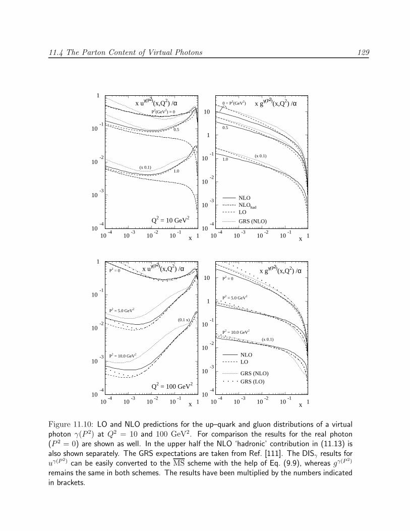
11.4 The Parton Content of Virtual Photons 129

Q2 = 10 GeV2

x

x uγ(P 2)(x,Q2) /αP2(GeV2) = 0

0.5

1.0(x 0.1)

NLONLOhadLO

GRS (NLO)

x

x gγ(P 2)(x,Q2) /α0 = P2(GeV2)

0.5

1.0(x 0.1)

10-4

10-3

10-2

10-1

1

10-4

10-3

10-2

10-1

110

-4

10-3

10-2

10-1

1

10

10-4

10-3

10-2

10-1

1

Q2 = 100 GeV2

x

x uγ(P 2)(x,Q2) /αP2 = 0

P2 = 5.0 GeV2

P2 = 10.0 GeV2

(0.1 x)

NLOLO

GRS (NLO)

GRS (LO)

x

x gγ(P 2)(x,Q2) /α

P2 = 0

P2 = 5.0 GeV2

P2 = 10.0 GeV2

(x 0.1)

10-4

10-3

10-2

10-1

1

10-4

10-3

10-2

10-1

110

-4

10-3

10-2

10-1

1

10

10-4

10-3

10-2

10-1

1

Figure 11.10: LO and NLO predictions for the up–quark and gluon distributions of a virtualphoton γ(P 2) at Q2 = 10 and 100 GeV2. For comparison the results for the real photon(P 2 = 0) are shown as well. In the upper half the NLO ‘hadronic’ contribution in (11.13) isalso shown separately. The GRS expectations are taken from Ref. [111]. The DISγ results foruγ(P 2) can be easily converted to the MS scheme with the help of Eq. (9.9), whereas gγ(P

2)

remains the same in both schemes. The results have been multiplied by the numbers indicatedin brackets.

11.4 The Parton Content of Virtual Photons 130

10-2

10-1

1

0 10 20 30 40 50 60 70 80

x f~ γ(P

2)(x,Q2) /α Q2 = 85 GeV2 , x = 0.425

P2/GeV2

x f~ γ(P

2)(x,Q2) /α Q2 = 85 GeV2 , x = 0.6

P2/GeV2

10-2

10-1

1

0 10 20 30 40 50 60 70 80

Figure 11.11: Predictions for the LO effective parton density xf γ(P 2)(x,Q2), defined in

Eq. (11.14), at the scale Q2 ≡(pjetT

)2= 85 GeV2 and at two fixed values of x. The

H1 data [157–161] have been extracted from DIS ep dijet production. The solid curves re-

fer to our predictions in the theoretically legitimate region P 2 ≪ Q2 ≡(pjetT

)2, whereas the

dashed curves extend into the kinematic region of larger P 2 approaching Q2 where the conceptof parton distributions of virtual photons is not valid anymore (see text).

11.5 Summary and Conclusions 131

11.5 Summary and Conclusions

The main purpose of the present chapter was to formulate a consistent set of boundary

conditions which allow for a perturbatively stable LO and NLO calculation of the photonic

parton distributions f γ(P 2)(x,Q2) as well as for a smooth transition to the parton densities

of a real (P 2 = 0) photon. Employing the pionic distributions fπ(x,Q2) of Chapter 10,

required for describing, via VMD, the nonpointlike hadronic components of a photon, we

arrive at essentially parameter–free predictions for f γ(P 2)(x,Q2) which are furthermore in

good agreement with all present measurements of the structure function F γ2 (x,Q

2) of real

photons γ ≡ γ(P 2 = 0). It should be noted that the experimentally almost unconstrained

pionic gluon and sea distributions, gπ(x,Q2) and q π(x,Q2), have been uniquely derived

from the experimentally rather well known pionic valence density vπ(x,Q2) and the (re-

cently updated [26] dynamical) parton distributions of the proton. We have furthermore

implemented these hadronic components by using a VMD ansatz for a coherent super-

position of vector mesons which maximally enhances the contributions of the up–quarks

to F γ2 as favored by all present data. Since these hadronic contributions are generated

from the valence–like input parton distributions at the universal target–mass independent

low resolution scale Q20 = µ2 ≃ 0.3 GeV2, we arrive, at least for real (P 2 = 0) photons,

at unique small–x predictions for x <∼ 10−2 at Q2 > µ2 which are of purely dynamical

origin, as in the case of hadrons. As has been demonstrated in Sec. 11.3 these small–x

predictions are in perfect agreement with recent small–x measurements of the photon

structure function F γ2 (x,Q

2) [98] at all presently accessible values of Q2. Furthermore,

since our universal input scale µ2 fixes also uniquely the perturbative pointlike part of

the photonic parton distributions, which dominates for x >∼ 0.1, the large–x behavior of

photonic structure functions is unambiguously predicted as well.

Our expectations for the parton content of virtual (P 2 6= 0) photons are clearly more

speculative, depending on how one models the hadronic component (input) of a vir-

tual photon. The latter is usually assumed to be similar to the VMD input for a real

photon, times a dipole suppression factor which derives from an effective vector–meson

P 2–propagator, cf. Eq. (11.12). Whenever a virtual photon is probed at a scale Q2 ≫ P 2,

with its virtuality being entirely taken care of by the (transverse) equivalent photon flux

factor and the boundary conditions for the photonic parton distributions, all cross sec-

tions of partonic subprocesses (resolved and direct) should be calculated as if P 2 = 0. In

11.5 Summary and Conclusions 132

other words, the treatment and expressions for f γ(P 2)(x,Q2) as on–shell transverse partons

obeying the usual RG Q2–evolution equations (with the usual splitting functions of real

photons, etc.) dictate an identification of the relevant sub–cross–sections f γ(P 2)X → X ′

with that of the real photon, σ(f γ(P 2)X → X ′) = σ(f γX → X ′). In particular, the

calculation of Fγ(P 2)2 (x,Q2) requires the same photonic Wilson coefficient Cγ(x) as for

P 2 = 0. This allows to formulate similar boundary conditions in LO and NLO which

give rise to perturbatively stable parton distributions, cross sections (i.e. also structure

functions) of virtual photons γ(P 2) as long as they are probed at scales Q2 ≫ P 2 where

Q2 ≡ 4m2c ,(pjetT

)2, etc., and typically P 2 <∼ 1

10Q2. It should be emphasized that only

in this latter kinematic range P 2 ≪ Q2 is the whole concept of RG resummed parton

distributions of (resolved) virtual photons appropriate and relevant. Parton distributions

of virtual photons extracted recently from DIS ep dijet data are in good agreement with

our (parameter–free) predictions.

Finally, we present simple analytic parametrizations of our predicted LO and

NLO(DISγ) parton distributions of real photons. From these LO parametrizations one

can easily obtain also the ones for a virtual photon which, whithin sufficient accuracy, may

also be used in NLO. Our NLO(DISγ) parametrizations of the parton densities of the real

photon can be easily transformed to the MS scheme according to Eq. (9.9) which might

be relevant for future NLO analyses of resolved photon contributions to hard processes

where most NLO subprocesses have so far been calculated in the MS scheme.

A FORTRAN package containing our most recent parametrizations can be obtained

by electronic mail on request.

Chapter 12

Has the QCD RG–Improved PartonContent of Virtual Photons beenObserved?

It is demonstrated that present e+e− and DIS ep data on the structure of the virtual

photon can be understood entirely in terms of the standard ‘naive’ quark–parton model

box approach. Thus the QCD renormalization group (RG) improved parton distributions

of virtual photons, in particular their gluonic component, have not yet been observed.

The appropriate kinematical regions for their future observation are pointed out as well

as suitable measurements which may demonstrate their relevance. The results presented

in this chapter are taken from [8].

12.1 Introduction

Recent measurements and experimental studies of dijet events in deep inelastic ep [161]

and of double–tagged e+e− [105] reactions have indicated a necessity for assigning a (QCD

resummed) parton content of virtual photons γ(P 2) as suggested and predicted theoreti-

cally [6, 97, 104, 111, 125–127, 153–155]. In particular the DIS dijet production data [161]

appear to imply a sizeable gluon component gγ(P2)(x,Q2) in the derived effective parton

density of the virtual photon, where Q2 refers to the hadronic scale of the process, Q ∼ pjetT ,

or to the virtuality of the probe photon γ∗(Q2) which probes the virtual target photon

γ(P 2) in e+e− → e+e−X . It is the main purpose of this chapter to demonstrate that this

is not the case and that all present data on virtual photons can be explained entirely in

12.2 RG–Improved Parton Model Expectations for the Effective Structure Function Feff 134

terms of the conventional QED doubly virtual box contribution γ⋆(Q2)γ⋆(P 2) → qq in

fixed order perturbation theory –sometimes also referred to as the quark–parton model

(QPM).

This is of course in contrast to the well known case of a real photon γ ≡ γ(P 2 ≡0) whose (anti–)quark and gluon content has been already experimentally established

(for recent reviews see [89, 90]) which result mainly from resummations (inhomogeneous

evolutions) of the pointlike mass singularities proportional to ln Q2/m2q occurring in the

box diagram of γ⋆(Q2)γ → qq for the light q = u, d, s quarks. This is in contrast to

a virtual photon target where γ⋆(Q2)γ⋆(P 2) → qq does not give rise to collinear (mass)

singularities but instead just to finite contributions proportional to ln Q2/P 2 which a

priori need not be resummed to all orders in QCD.

This chapter is organized as follows:

In Sec. 12.2 we compare fixed order box and QCD resummed expectations for the effective

structure function Feff with present e+e− data, while Sec. 12.3 contains a comparison of an

effective leading order parton density for the virtual photon with DIS ep data. Suggestions

of experimental signatures which can probe the QCD parton content, in particular the

gluon content of virtual photons are presented in Sec. 12.4 and our conclusions are finally

drawn in Section 12.5.

12.2 RG–Improved Parton Model Expectations for

the Effective Structure Function Feff

As promised in Chap. 8 we shall now turn to a quantitative study of the various QED–

box and QCD Q2–evoluted structure function expectations for a virtual photon target

and confront them with all presently available e+e− data of PLUTO [106] and the recent

one of LEP–L3 [105]. The ’asymptotic’ and ’full’ box results for Feff have already been

presented in Chap. 8 and details of their calculation can be found there. The QCD

resummed expectations for Feff according to our model in the previous chapter are given

by

Feff(x,Q2, P 2) = F

γ(P 2)2 (x,Q2) (12.1)

since we neglect any effects due to longitudinal target photons in our approach [6].

12.2 RG–Improved Parton Model Expectations for the Effective Structure Function Feff 135

Q2 = 5.0 GeV2 , P2 = 0.35 GeV2

F eff(

x,Q

2 ,P2 )/

α

x

full boxasympt. boxcharm (full box)GRSc (NLO)SaS 1D

F2

0

0.1

0.2

0.3

0.4

0.5

0.6

0.7

0.8

0.9

1

0 0.1 0.2 0.3 0.4 0.5 0.6 0.7 0.8 0.9 1

Figure 12.1: Predictions for Feff as defined in (8.14). The box results are as in Fig. 8.3.The QCD resummed NLO expectations of GRSc [6] for F2 in (12.1) turn out to be similarto the LO ones [6]. Also shown are the LO–resummed results of SaS 1D [97] for F2 andFeff = F2 +

32FLT (see text). The total charm contribution to the latter two QCD results

involves also a ‘resolved’ component Fγ(P 2),res2,h

(x,Q2) according to Eq. (9.14) which turns outto be small as compared to the box contribution shown which dominates in the kinematicregion considered. The PLUTO data are taken from [106].

12.2 RG–Improved Parton Model Expectations for the Effective Structure Function Feff 136

Q2 = 120 GeV2 , P2 = 3.7 GeV2F ef

f(x,

Q2 ,P

2 )/α

x

full boxasympt. boxcharm (full box)GRSc (NLO)SaS 1D

0

0.25

0.5

0.75

1

1.25

1.5

1.75

2

2.25

2.5

0.1 0.2 0.3 0.4 0.5 0.6 0.7 0.8 0.9 1

Figure 12.2: As in Fig. 12.1, but for Q2 = 120 GeV2 and P 2 = 3.7 GeV2 appropriate for theLEP–L3 data [105].

A different approach has been suggested by Schuler and Sjostrand [97]. Apart from

using somewhat different input scales Q0 and parton densities, the perturbatively exactly

calculable box expressions for Λ2 ≪ P 2 ≪ Q2 (cf. App. C.2) are, together with their

LO–QCD Q2–evolutions, extrapolated to the case of real photons P 2 = 0 by employing

some dispersion–integral–like relations. These link perturbative and non–perturbative

contributions and allow a smooth limit P 2 → 0. (Note, however, that the LO Q2–

evolutions are performed by using again the splitting functions of real photons and on–

shell partons.) Since one works here explicitly with virtual (P 2 6= 0) expressions, the

longitudinal contributions of the virtual photon target should be also taken into account

when calculating Feff = F2 +32xFLT with Fab ≡ Q2/(4π2α)(xβ)−1σab (a = (L,T), b =

(L,T)) and where σab is given in Eq. (8.11), as described for example in [111], which is in

contrast to our approach in (12.1).1

1In an alternative approach [130, 132] one may consider the longitudinal component of the virtualphoton target γL(P

2) to possess, like the transverse component, a universal process independent hadroniccontent obtained radiatively via the standard homogeneous (Altarelli–Parisi)Q2–evolution equations withthe boundary conditions for the pointlike component at Q2 = P 2 given in Eq. (9.55). We have checkedthat the predictions for Feff(x,Q

2, P 2) obtained in this approach differ only slightly (typically about 10%or less) from those of the standard fixed order perturbative approach at presently relevant kinematicalregions (P 2 <∼ 1

10Q2, x >∼ 0.05) due to the smallness of F ℓ

TL relative to F ℓTT deriving from σℓ

TL and σℓTT,

respectively, in (8.17).

12.3 Comparison with DIS ep Data and Effective Quark Distributions 137

Despite the limited statistics of present data the box predictions for Feff in (8.14) shown

in Figs. 12.1 and 12.2 appear to be in even better agreement with present measurements

than the QCD resummed expectations of SaS [97] and GRSc [6]. Typical QCD effects

like the increase in the small–x region in Fig. 12.1, being partly caused by the presence of

a finite gluon content gγ(P2)(x,Q2), cannot be delineated with the present poor statistics

data.

These results clearly demonstrate that the naive QPM predictions derived from the

doubly virtual box γ⋆(Q2)γ⋆(P 2) → qq fully reproduce all e+e− data on the structure of

virtual photons γ(P 2). In other words, there is no sign of a QCD resummed parton content

in virtual photons in present data, in particular of a finite gluon content gγ(P2)(x,Q2)

which is absent in the ‘naive’ box (QPM) approach.

Characteristic possible signatures for QCD effects which are caused by the presence

of a finite and dominant gluon component gγ(P2) will be discussed in Sec. 12.4.

12.3 Comparison of Theoretical Expectations with

DIS ep Data and Effective Quark Distributions

of Virtual Photons

In oder to extract the parton densities of virtual photons from DIS ep dijet data, the H1

collaboration [161] has adopted the ‘single effective subprocess approximation’ [183] which

exploits the fact that the dominant contributions to the cross section in LO–QCD comes

from the 2 → 2 parton–parton hard scattering subprocesses that have similar shapes and

thus differ mainly by their associated color factors. Therefore the sum over the partonic

subprocesses can be replaced by a single effective subprocess cross section and effective

parton densities for the virtual photon given by

f γ(P 2)(x,Q2) =∑

q=u, d, s

[qγ(P

2)(x,Q2) + q γ(P 2)(x,Q2)]+

9

4gγ(P

2)(x,Q2) (12.2)

with a similar relation for the proton f p(x,Q2) which is assumed to be known. It should

be emphasized that such an effective procedure does not hold in NLO where all additional

(very different) 2 → 3 subprocesses contribute [164]. This NLO analysis affords therefore

a confrontation with more detailed data on the triple–differential dijet cross section as

compared to presently available data [161] which are not yet sufficient for examining the

12.3 Comparison with DIS ep Data and Effective Quark Distributions 138

10-2

10-1

1

0 10 20 30 40 50 60 70 80

x f~ γ(P

2)(x,Q2) /α Q2 = 85 GeV2 , x = 0.425

η(P2) x f~ γ(x,Q2) /α

H1 dijet data

P2/GeV2

effectiveQCDbox

x f~ γ(P

2)(x,Q2) /α Q2 = 85 GeV2 , x = 0.6

η(P2) x f~ γ(x,Q2) /α

P2/GeV2

10-2

10-1

1

0 10 20 30 40 50 60 70 80

Figure 12.3: Predictions for the effective parton density defined in Eq. (12.2). The ‘box’ results

refer to the universal qγ(P 2)box in (12.3), and the ‘effective’ ones to q

γ(P 2)eff as defined in (12.4)

as derived from the full box expressions (8.11) including all O(P 2/Q2) contributions. TheLO–QCD predictions of GRSc [6] are shown by the solid curves which refer to the predictionsin the theoretically legitimate region P 2 ≪ Q2, whereas the dashed curves extend into thekinematic region of larger P 2 approaching Q2 where the concept of QCD–resummed partondistributions of virtual photons is not valid anymore. (Note that the results for x = 0.6terminate at P 2 ≃ 54 GeV2 due to the kinematic constraint W 2 > 0, with W 2 being definedin (7.1), i.e. x < (1+P 2/Q2)−1.) For illustration we also show the effective LO–QCD partondensity f γ of a real photon γ ≡ γ(P 2 = 0) of GRSc [6] multiplied by the simple ρ–polesuppression factor η(P 2) in (11.12) which clearly underestimates the H1–data [161].

12.3 Comparison with DIS ep Data and Effective Quark Distributions 139

relative contributions of qγ(P2)(x,Q2) and gγ(P

2)(x,Q2). In Fig. 12.3 we compare our

LO RG–resummed predictions for f γ(P 2)(x,Q2) with the naive non–resummed universal

(process independent) box expressions [cf. Sec. 9.3.4]

qγ(P 2)box (x,Q2) = q

γ(P 2)box (x,Q2) = 3e2q

α

2π

[x2 + (1− x)2

]ln

Q2

P 2. (12.3)

Although the fully QCD–resummed results are sizeable and somewhat larger in the small

P 2 region than the universal box expectations, present H1 data [161] at Q2 ≡ (pjetT )2 = 85

GeV2 cannot definitely distinguish between these predictions. It should be furthermore

noted that the QCD gluon contribution gγ(P2)(x,Q2) is suppressed at the large values of

x shown in Fig. 12.3. Therefore present data [161] cannot discriminate between the finite

QCD resummed component gγ(P2)(x,Q2) and the non–resummed g

γ(P 2)box (x,Q2) = 0.

It is obvious that these two results shown in Fig. 12.3 are only appropriate for vir-

tualities P 2 ≪ Q2, typically P 2 = 10 to 20 GeV2 at Q2 = 85 GeV2, since O(P 2/Q2)

contributions are neglected in RG–resummations as well as in the definition (12.3). In or-

der to demonstrate the importance of O(P 2/Q2) power corrections in the large P 2 region

let us define, generalizing the definition (9.34), some effective (anti)quark distributions as

common via

1

xF ℓ2,box(x,Q

2) ≡∑

q=u, d, s

e2q

[qγ(P 2)eff (x,Q2) + q

γ(P 2)eff (x,Q2)

](12.4)

where, of course, qγ(P 2)eff = q

γ(P 2)eff and the full box expression for F ℓ

2,box(x,Q2) can be ob-

tained from the general definition in Eq. (7.25) and the full box results in Eq. (8.11)

utilizing m ≡ mq = 0, i.e. λ = 0 and summing over the light quarks. The full box expres-

sions imply again gγ(P 2)eff (x,Q2) = 0 in contrast to the QCD resummed gluon distribution.

The qγ(P 2)eff introduced in (12.4) is, in contrast to (12.3), of course non–universal. The

‘effective’ results shown in Fig. 12.3 clearly demonstrate the importance of the O(P 2/Q2)

terms at larger values of P 2 <∼ Q2 which are not taken into account by the QCD re-

summations and by the universal box expressions in (12.3) also shown in Fig. 12.3. It is

interesting that the non–universal qγ(P 2)eff defined via F2 in (12.4) describes the H1–data

at large values of P 2 in Fig. 12.3 remarkably well. This may be accidental and it remains

to be seen whether future LO analyses will indicate the general relevance of qγ(P 2)eff (x,Q2)

in the large P 2 region.

As we have seen, present DIS dijet data cannot discriminate between the universal

naive box and QCD–resummed expectations in the theoretically relevant region P 2 ≪ Q2,

12.4 Possible Signatures for the QCD Parton Content of Virtual Photons 140

F 2 c (x,Q

2 ,P2 )/

α

x

Q2 = 100 GeV2 , P2 = 1 GeV2

direct (box)

resolved

0

0.02

0.04

0.06

0.08

0.1

0.12

0.14

10-2

10-1

Figure 12.4: Expected charm contributions to F2. The naive ‘direct (box)’ result refers to(9.13) [or (C.12)] and the LO–QCD ‘resolved’ prediction is given in (9.14) with gγ(P

2)(x, 4m2c)

taken from GRSc [6]. This latter ‘resolved’ contribution is absent in the naive box (QPM)approach.

mainly because these data are insensitive to the gluon content in γ(P 2) generated by

QCD–evolutions which is absent within the naive box approach. Therefore we finally

turn to a brief discussion where such typical QCD effects may be observed and delineated

by future experiments.

12.4 Possible Signatures for the QCD Parton Con-

tent of Virtual Photons

Since e+e− and DIS ep dijet data cannot, at present, delineate the QCD–resummed parton

content of a virtual photon, in particular not its gluon content, we shall now propose and

discuss a few cases where such typical QCD effects may be observed and possibly confirmed

by future experiments.

Charm production in e+e− → e+e− ccX would be a classical possibility to delineate

such effects due to a nonvanishing gγ(P2)(x,Q2). In Fig. 12.4 we compare the usual (fixed

12.4 Possible Signatures for the QCD Parton Content of Virtual Photons 141

x

Q2 = 85 GeV2 , P2 = 1 GeV2

9-4 xgγ(P 2)/α

xΣbox γ(P

2)/α

xΣeff γ(P

2)/α xΣγ(P 2)/α

0

0.1

0.2

0.3

0.4

0.5

0.6

0.7

0.8

0.9

1

0 0.1 0.2 0.3 0.4 0.5 0.6

x

Q2 = 85 GeV2 , P2 = 5 GeV2

9-4 xgγ(P 2)/α

xΣbox γ(P

2)/α

xΣeff γ(P

2)/α

xΣγ(P 2)/α

0

0.1

0.2

0.3

0.4

0.5

0.6

0.7

0.8

0.9

1

0 0.1 0.2 0.3 0.4 0.5 0.6

Figure 12.5: Predictions for the total light quark Σγ(P 2) ≡ 2Σq=u, d, s qγ(P 2) and gluon contri-

butions to the effective parton density in (12.2) at a fixed scale Q2 = 85 GeV2 and two fixed

virtualities P 2 = 1 and 5 GeV2. The naive box results refer to the universal qγ(P 2)box defined in

(12.3) and to qγ(P 2)eff defined in (12.4). The LO–QCD RG–resummed predictions are denoted

by Σγ(P 2) and gγ(P2) according to GRSc [6]. The latter gluon contribution is absent in the

naive box (QPM) approach.

12.4 Possible Signatures for the QCD Parton Content of Virtual Photons 142

order) ‘direct’ box contribution to F c2 with the ‘resolved’ gluon–initiated one as given by

(9.14). The ‘direct’ box contribution entirely dominates in the large–x region, x >∼ 0.05,

accessible by present experiments (cf. Figs. 12.1 and 12.2), whereas the typical QCD–

resummed ‘resolved’ contribution becomes comparable to the ‘direct’ one and eventually

dominates in the small–x region, x < 0.05. Thus a careful measurement of the charm

contribution to F2 at x <∼ 0.05 would shed some light on the QCD parton (gluon) content

of virtual photons, since such a ‘resolved’ contribution in Fig. 12.4 would be absent within

the naive box approach.

The effective parton distribution f γ(P 2)(x,Q2) in (12.2) at not too large values of x

and P 2, as may be extracted in LO from DIS ep dijet data, would be another possibility to

observe QCD–resummation effects due to a nonvanishing gluon component gγ(P2)(x,Q2).

In Fig. 12.5 we show the quark and gluon contributions to f γ(P 2) in (12.2) separately. The

box (anti–)quark contributions, which are similar to the QCD–resummed ones, entirely

dominate over the QCD–resummed gluon contribution in the large–x region, x >∼ 0.4,

accessible to present experiments (cf. Fig. 12.3). Only below x ≃ 0.3 does the QCD gluon

contribution become comparable to the (anti–)quark components and dominates, as usual,

for x <∼ 0.1. It should be remembered that gγ(P 2)box (x,Q2) = 0. Furthermore, the increase of

the RG–resummed qγ(P2)(x,Q2) at small x in Fig. 12.5 is induced by the vector–meson–

dominance–like input for the Q2–evolution of the ‘hadronic’ component of the photon’s

parton distribution [6, 97] and is disregarded in our naive box (QPM) analysis.

Thus a measurement of dijets produced in DIS ep reactions in the not too large x

region, x <∼ 0.3, would probe the QCD parton content of virtual photons, in particular

their gluon content which is absent in the naive QPM box approach. In this region,

and at not too large photon virtualities P 2 <∼ 5 GeV2 shown in Fig. 12.5, the ‘resolved’

gluon–dominated contribution of the virtual photon to high ET jet production at scales

Q ≡ ET ≃ 5 − 10 GeV exceeds by far the ‘direct’ box–like contribution of a pointlike

virtual photon [162]. The production of prompt photons at HERA via a tagged DIS

process ep → eγX may offer additional probes of the gluonic content of virtual photons

[184].

12.5 Summary and Conclusions 143

12.5 Summary and Conclusions

Virtual photons γ(P 2), probed at a large scale Q2 ≫ P 2, may be described either by

fixed order perturbation theory, which in lowest order of QCD yield the quarks and

anti–quarks generated by the universal part of the ‘box’ diagram, or alternatively by

their renormalization group (RG) improved counterparts including particularly the gluon

distribution gγ(P2)(x,Q2).

The results in Sections 12.2 and 12.3 demonstrate that all presently available e+e−

and DIS ep dijet data can be fully accounted for by the standard doubly virtual QED

box diagram and are not yet sensitive to RG resummation effects which are manifest only

in the presently unexplored low–x region of the parton distributions in γ(P 2). In fact,

as shown in Section 12.4, these resummation effects start to dominate only at x < 0.3

and may be observed by future measurements at P 2 = O(1 GeV2) of σ(ep → e jjX)

or σ(e+e− → e+e− ccX) at high energy collisions. These measurements could finally

discriminate between the fixed order and RG–improved parton distributions of the virtual

photon.

Chapter 13

Summary

It was the main theme of Part II of this thesis to analyze the parton content of pions and

real and virtual photons in leading order (LO) and next–to–leading order (NLO) of QCD

within the framework of the recently updated [26] radiative parton model [26, 41, 57, 92,

93].

We started with a detailed consideration of the ee → eeX scattering process being

presently the main source of information on the structure of real and virtual photons. We

defined structure functions for virtual photons in a model independent way and related

them to the photon–photon scattering cross sections. These structure functions can be

measured in deep inelastic electron–photon scattering (DISeγ) and we demonstrated the

factorization of the cross section for the process ee → eeX into a flux of photons (produced

by bremsstrahlung off the incident lepton) times the DISeγ cross section for the general

P 2 6= 0 case in the Bjorken limit P 2 ≪ Q2. However, we found that the neglected terms

are of the order O(√

xP 2/Q2) only and not of the order O(xP 2/Q2) as might have been

naively expected. Clearly, a numerical comparison of the factorization formula with the

exact ee → eeX cross section would be interesting in order to clarify when xP 2/Q2 is

small enough such that the factorization formula is a good approximation.

From these general kinematical considerations we turned to a calculation of the

photon–photon cross sections σab according to the doubly virtual box γ⋆(Q2)γ⋆(P 2) → qq

in lowest order perturbation theory. We utilized these results in order to compute the ef-

fective structure function Feff(x,Q2, P 2) in fixed order perturbation theory (FOPT) which

we compared with all present e+e− virtual photon data [105, 106]. It came out that the

LO–box predictions for Feff are in agreement with the present low statistics data even in

145

the case of the PLUTO data [106] with P 2 = 0.35 GeV2 which is just in the transition

region from deeply virtual (P 2 ≫ Λ2) to real (P 2 ≃ 0) photons where non–perturbative

effects are expected to become increasingly important, especially in the small–x region.

More precise data for Feff in this ’transition region’ with intermediate target virtualities

would be highly desirable in order to observe the onset of such non–perturbative effects.

On the other hand, NLO corrections to the doubly virtual box [108] offer the possibility to

investigate the perturbative stability of the fixed order results and to see if the description

of the data further improves in NLO accuracy.

After presenting the complete theoretical framework we started our phenomenological

studies of radiatively generated parton distributions with an analysis of the parton content

of the pion in LO and NLO QCD. Since only the pionic valence density vπ(x,Q2) is

experimentally rather well known at present, we utilized a constituent quark model [94, 95]

in order to unambiguously relate the pionic light sea q π(x,Q2) and gluon gπ(x,Q2) to the

much better known (recently updated) parton distributions of the proton [26] and the

pionic valence density vπ(x,Q2).

Next we formulated a consistent set of boundary conditions which allowed for a pertur-

batively stable LO and NLO calculation of the photonic parton distributions f γ(P 2)(x,Q2)

as well as for a smooth transition to the parton densities of a real (P 2 = 0) photon. Em-

ploying the above summarized pionic distributions fπ(x,Q2), required for describing –via

vector meson dominance (VMD)– the nonpointlike hadronic components of a photon, we

arrived at essentially parameter–free predictions for f γ(P 2)(x,Q2) which turned out to be

in good agreement with all present measurements of the structure function F γ2 (x,Q

2) of

real photons γ ≡ γ(P 2 = 0). More specifically, we implemented these hadronic com-

ponents by using a VMD ansatz for a coherent superposition of vector mesons which

maximally enhances the contributions of the up–quarks to F γ2 (x,Q

2) as favored by all

present data. Since these hadronic contributions are generated from the valence–like in-

put parton distributions at the universal target–mass independent low resolution scale

Q20 = µ2 ≃ 0.3 GeV2, we arrived, at least for real (P 2 = 0) photons, at unique small–x

predictions for x <∼ 10−2 at Q2 > µ2 which are of purely dynamical origin, as in the case of

hadrons. A comparison with most recent small–x measurements of the photon structure

function F γ2 (x,Q

2) [98] showed that these small–x predictions are in perfect agreement

with the data at all presently accessible values of Q2. The agreement with the data on

F γ2 (x,Q

2) confirms our radiatively generated quark distributions qγ(x,Q2) = qγ(x,Q2)

146

while the gluon is probed only indirectly at small–x due to the evolution. It would be also

interesting and important to extend present measurements [89, 90, 180, 181] of the gluon

distribution of the photon, gγ(x,Q2), below the presently measured region 0.1 <∼ x < 1

where gγ(x < 0.1, Q2) is expected to be somewhat flatter in the small–x region than

previously anticipated [96]. Our expectations for the parton content of virtual (P 2 6= 0)

photons are clearly more speculative, depending on how one models the hadronic com-

ponent (input) of a virtual photon. We assumed the latter to be similar to the VMD

input for a real photon times a dipole suppression factor which derives from an effective

vector–meson P 2–propagator representing somehow the simpliest choice. We formulated

similar boundary conditions in LO and NLO which gave rise to perturbatively stable

parton distributions and cross sections (i.e. also structure functions of virtual photons)

as long as they are probed at scales Q2 ≫ P 2 where Q2 is a hard scale of the process

under consideration. We showed that effective parton distributions of virtual photons ex-

tracted recently from DIS ep dijet data are in good agreement with our (parameter–free)

predictions.

Finally, we turned to more detailed tests of our model for the parton content of virtual

photons and we compared these QCD–resummed expectations with the above summarized

fixed order box expressions. Our results demonstrated that all presently available e+e−

and DIS ep dijet data can be fully accounted for by the standard doubly virtual QED

box diagram and are not yet sensitive to RG resummation effects which are manifest

only in the presently unexplored low–x region of the parton distributions in γ(P 2). It

turned out that these resummation effects start to dominate only at x . 0.3 (the larger

P 2 the smaller x) and may be observed by future measurements at P 2 = O(1 GeV2) of

σ(ep → e jjX) or σ(e+e− → e+e− ccX) at high energy collisions. These measurements

could finally discriminate between the fixed order and RG–improved parton distributions

of the virtual photon.

FORTRAN packages containing simple analytic parametrizations of our most recent

parton distributions of the pion and the (real and virtual) photon are available upon

request by electronic mail from schien@zylon.physik.uni-dortmund.de.

Appendix A

Deep Inelastic Scattering on MassiveQuarks at O(α1s)

A.1 Real Gluon Emission

We define a partonic tensor

ωµν ≡∑

color

∑

spin

〈Q2(p2), g(k)∣∣Q2γ

µ(V − Aγ5)Q1

∣∣Q1(p1)〉 × 〈µ → ν〉∗ (A.1)

which can be decomposed into its different tensor components as usual

ωµν = −ωQ1 gµν + ωQ

2 pµ1pν1 + iωQ

3 ε µναβ pα1 q

β + ωQ4 qµqν + ωQ

5 (qµpν1 + qνpµ1 ) . (A.2)

ωµν can be easily calculated from the general Feynman rules for invariant matrix elements

which are customarily expressed as functions of the Mandelstam variables s ≡ (p1 + q)2

and t ≡ (p1 − k)2 to which we will refer in the following. Projection onto the individual

ωQi=1,2,3 in Eq. (A.2) is performed for nonzero masses and in n = 4 + 2ε dimensions with

the following operators

P µν1 =

−1

2(1 + ε)

{gµν +

[m2

1 qµqν −Q2 pµ1 pν1 − (p1 · q)(qµpν1 + pµ1qν)]

× 4∆−2[m21, s,−Q2]

}

P µν2 = 2

[− gµνQ2 + 4 qµqν

2(1 + ε)(p1 · q)2 −m21Q

2

∆2[m21, s,−Q2]

+ 4(3 + 2ε)Q2 Q2 pµ1pν1 + (p1 · q)(qµpν1 + pµ1q

ν)

∆2[m21, s,−Q2]

] {(1 + ε)∆2[m2

1, s,−Q2]}−1

P µν3 =

−2i

∆2[m21, s,−Q2]

εµνλκ pλ1 qκ (A.3)

A.1 Real Gluon Emission 148

such that Pi · ω = ωQi . The normalization in Eqs. (A.1), (A.2) is such that real gluon

emission contributes FRi to the hadronic structure functions via

FR1 =

1

8π

∫ 1

χ

dξ

ξQ1(ξ)

∫dPS ωQ

1

FR2 =

2x

16π

∫ 1

χ

dξ

ξ

∆2[m21, s,−Q2]

2Q2Q1(ξ)

∫dPS ωQ

2

FR3 =

1

8π

∫ 1

χ

dξ

ξ∆[m2

1, s,−Q2] Q1(ξ)

∫dPS ωQ

3 (A.4)

where [185]

∫dPS =

1

8π

s−m22

s

1

Γ(1 + ε)

[(s−m2

2)2

4πs

]ε ∫ 1

0

[y(1− y)]ε dy (A.5)

is the partonic phase space. In Eq. (A.5) y is related to the partonic center of mass

scattering angle θ∗ and the partonic Mandelstam variable t via

y ≡ 1

2(1 + cos θ∗)

=1

2∆[m21, s,−Q2]

[Q2 +m2

1 + s+∆[m21, s,−Q2] +

2s(t−m21)

s−m22

]. (A.6)

We have chosen dimensional regularization for the soft gluon poles stemming from s → m22

which arise from propagators in the ωi times phase space factors in dPS. In Eq. (A.4) we

use [48]

(s−m22)

2ε−1 ∼(1− χ

ξ

)2ε−1

=1

2εδ(1− χ/ξ) +

1

(1− χ/ξ)++O(ε) (A.7)

which separates hard gluon emission (∼ fQi ) from soft gluon (Si) contributions in Eq.

(3.10). Note that in Eqs. (3.9), (3.10) the integration variable ξ, which is implicitly defined

in Eq. (3.2), has been changed to ξ′ ≡ χ/ξ for an easier handling of the distributions. For

the relation between s and ξ′ see Eq. (A.39) below.

Since all quark masses are kept nonzero, no poles in y (collinear singularities) are

contained in the integration volume. The fQi which occur in Eq. (3.10) and which are

given below in Eq. (A.40) are therefore straightforward integrals of the ωQi

fQi =

(g2s CF

)−1∫ 1

0

dy ωQi (A.8)

A.2 Vertex Correction 149

and the Si in Eqs. (3.10), (A.37) pick up the pole in Eq. (A.7)

Si ∼1

ε

∫ 1

0

dy [y(1− y)]ε[ωQi (s−m2

2)2]∣∣∣

ξ=χ, (A.9)

where the proportionality is given by kinematical and phase space factors which must be

kept up to O(ε).

The normalization of our hadronic structure functions in Eq. (A.4) can be clearly

inferred from the corresponding LO results in Eq. (3.3). Nevertheless, for definiteness we

also give the hadronic differential cross section to which it corresponds

d2σl,l

dxdy=

1

nl

(GB,B′

l )2 (GB,B′

q )2 2MNEl

2π

×[Sl,+ (1− y)F2 + Sl,+ y2xF1 ±Rl,+ 2y(1− y

2)xF3

], (A.10)

where (GB,B′

l,q )2 = [gBl,q2/(Q2 + M2

B) gB′

l,q

2/(Q2 + M2

B′)]1/2 is the effective squared gauge

coupling –including the gauge boson propagator– of the γµ(V − Aγ5) lepton and quark

current, respectively, and nl counts the spin degrees of freedom of the lepton, e.g. nl = 1, 2

for l = ν, e−. The leptonic couplings Sl,+, Rl,+ are defined analogous to the quark couplings

in Eq. (3.6). As noted below Eq. (3.6), B = B′ for non–interference (pure B scattering).

A.2 Vertex Correction

A.2.1 Results

We have calculated the vertex correction in n = 4 + 2ε dimensions at O(α1s) for gen-

eral masses and couplings using the Feynman gauge. The unrenormalized vertex Λµ0

[Fig. 3.1(c.1)] has the structure

Λµ0 = CF

αs

4πΓ(1− ε)

(Q2

4πµ2

)ε{C0,− γµL5 + C+ γµR5

+ C1,− m2 pµ1 L5 + C1,+ m1 pµ1 R5 + Cq,− m2qµ L5 + Cq,+ m1q

µ R5

}(A.11)

with L5 = (V −A γ5), R5 = (V + A γ5). The coefficients read

C0,− =1

ε(−1 − Σ++I1) +

[∆2

2Q2+ Σ++

(1 + ln

(Q2

∆

))]I1

A.2 Vertex Correction 150

+1

2ln

(Q2

m21

)+

1

2ln

(Q2

m22

)+

m22 −m2

1

2Q2ln

(m2

1

m22

)+

Σ++

∆(A.12)

×{1

2ln2

∣∣∣∣∆− Σ+−

2Q2

∣∣∣∣+1

2ln2

∣∣∣∣∆− Σ

−+

2Q2

∣∣∣∣−1

2ln2

∣∣∣∣∆+Σ+−

2Q2

∣∣∣∣−1

2ln2

∣∣∣∣∆+Σ

−+

2Q2

∣∣∣∣

− Li2

(∆− Σ+−

2∆

)− Li2

(∆− Σ

−+

2∆

)+ Li2

(∆+Σ+−

2∆

)+ Li2

(∆+Σ

−+

2∆

)}

C+ = 2m1m2I1

C1,− =−1

Q2

[Σ+−

I1 + ln

(m2

1

m22

)]

C1,+ =−1

Q2

[Σ

−+I1 − ln

(m2

1

m22

)]

Cq,− =1

Q4

[(∆2 − 2m2

1Q2)I1 − 2Q2 + Σ+−

ln

(m2

1

m22

)]

Cq,+ =1

Q4

[(−∆2 + 2m2

2Q2 − Σ

−+Q2)I1 + 2Q2 + (Σ

−+ +Q2) ln

(m2

1

m22

)](A.13)

with

I1 =1

∆ln

[Σ++ +∆

Σ++ −∆

](A.14)

I2 = I1 ln∆− 1

∆(A.15)

×{1

2ln2

∣∣∣∣∆− Σ+−

2Q2

∣∣∣∣+1

2ln2

∣∣∣∣∆− Σ

−+

2Q2

∣∣∣∣−1

2ln2

∣∣∣∣∆+Σ+−

2Q2

∣∣∣∣−1

2ln2

∣∣∣∣∆+Σ

−+

2Q2

∣∣∣∣

− Li2

(∆− Σ+−

2∆

)− Li2

(∆− Σ

−+

2∆

)+ Li2

(∆+Σ+−

2∆

)+ Li2

(∆+Σ

−+

2∆

)}.

The renormalized vertex [Fig. 3.1 (c.1)–(c.3)] is obtained by wave function renormal-

ization:

ΛµR = γµL5(Z1 − 1) + Λµ

0 +O(α2s) (A.16)

where Z1 =√

Z2(p1)Z2(p2). The fermion wave function renormalization constants are

defined on mass shell:

Z2(mi) = 1 + CFαs

4πΓ(1− ε)

(m2

i

4πµ2

)ε1

ε[3− 4ε+O(ε2)] (A.17)

such that

Z1 = 1 + CFαs

4πΓ(1− ε)

(Q2

4πµ2

)ε [3

ε− 3

2ln

(Q2

m21

)− 3

2ln

(Q2

m22

)− 4

]. (A.18)

A.2 Vertex Correction 151

The final result for the renormalized vertex ΛµR reads

ΛµR = CF

αs

4πΓ(1− ε)

(Q2

4πµ2

)ε{CR,−γ

µL5 + C+γµR5

+ C1,− m2 pµ1 L5 + C1,+ m1 pµ1 R5 + Cq,− m2 qµ L5 + Cq,+ m1 qµ R5

}(A.19)

with C+, C1,±, Cq,± as given above and

CR,− =1

ε(2− Σ++I1) +

[∆2

2Q2+ Σ++

(1 + ln

(Q2

∆

))]I1 (A.20)

+m2

2 −m21

2Q2ln

(m2

1

m22

)− ln

(Q2

m21

)− ln

(Q2

m22

)− 4 +

Σ++

∆

×{1

2ln2

∣∣∣∣∆− Σ+−

2Q2

∣∣∣∣ +1

2ln2

∣∣∣∣∆− Σ

−+

2Q2

∣∣∣∣−1

2ln2

∣∣∣∣∆+Σ+−

2Q2

∣∣∣∣−1

2ln2

∣∣∣∣∆+Σ

−+

2Q2

∣∣∣∣

− Li2

(∆− Σ+−

2∆

)− Li2

(∆− Σ

−+

2∆

)+ Li2

(∆+Σ+−

2∆

)+ Li2

(∆+Σ

−+

2∆

)}.

A.2.2 Calculation

Basic ingredient in the calculation of one–loop virtual corrections are one–loop integrals

classified according to the number N of propagator factors in the denominator and the

number P of integration momenta in the numerator. Integrals with N = 1, 2, 3, 4 are

usually called one–, two–, three– and four–point functions (1PF . . . 4PF). For P+4−2N ≥0 these integrals are UV–divergent. In dimensional regularization these divergences are

regulated by evaluating the integrals in general dimensions n 6= 4 and the divergences

become manifest as poles in the limit n → 4.

We define the following one–loop tensor integrals1 (see for example [186, 187]):

TNµ1···µP

(p1, . . . , pN−1, m0, . . . , mN−1) ≡(2πµ)4−n

iπ2

∫dnl

lµ1 · · · lµP

D0D1 · · ·DN−1(A.21)

where all the external momenta pi are defined to be incoming and the denominators

stemming from the propagators in the Feynman diagram are given by

Di = (l + pi)2 −m2

i + iε , with pi ≡i∑

j=1

pj , (i = 0, . . . , N − 1) . (A.22)

1Note that this definition is related to Eq. (4.1) in [186] as follows:

TNµ1···µP

(p1, . . . , pN−1,m0, . . . ,mN−1) = TN,Dennerµ1···µP

(p1, . . . , pN−1,m0, . . . ,mN−1).

A.2 Vertex Correction 152

To achieve a cyclic symmetry we furthermore identify the 0–th with the N–th propagator:

DN ≡ D0, mN ≡ m0 and pN = p0 = 0. Furthermore it is convenient to define

pi0 = pi , pij = pi − pj . (A.23)

The +iε part in the denominators with an infinitesimal ε > 0 is needed to regulate

singularities of the integrand and its specific choice ensures causality. After integration it

determines the correct imaginary parts of the logarithms and dilogarithms. The arbitrary

mass scale µ has been introduced such that the integrals have an integer mass dimension.

Conventionally TN is denoted by the N–th character of the alphabet, i.e. T 1 ≡ A,

T 2 ≡ B, . . . , and the scalar integrals carry an index 0.

The tensor integrals in (A.21) can be related to the scalar integrals A0, B0, C0 and

D0 by a Passarino–Veltman decomposition [188] which will be described in the following.

Due to Lorentz covariance the tensor integrals (A.21) can be decomposed into tensors

constructed from the external momenta pi and the metric tensor gµν . The choice of the

tensor basis is not unique and we will stick to the following form [187, 189]:

Bµ = pµ1B1

Bµν = pµ1pν1B21 + gµνB22

Cµ = pµ1C11 + pµ2C12

Cµν = pµ1pν1C21 + pµ2p

ν2C22 + {p1p2}µνC23 + gµνC24

Cµνρ = pµ1pν1p

ρ1C31 + pµ2p

ν2p

ρ2C32 + {p1p1p2}µνρC33 + {p1p2p2}µνρC34

+ {p1g}µνρC35 + {p2g}µνρC36

Dµ = pµ1D11 + pµ2D12 + pµ3D13

Dµν = pµ1pν1D21 + pµ2p

ν2D22 + pµ3p

ν3D23 + {p1p2}µνD24 + {p1p3}µνD25

+ {p2p3}µνD26 + gµνD27

Dµνρ = pµ1pν1p

ρ1D31 + pµ2p

ν2p

ρ2D32 + pµ3p

ν3p

ρ3D33 + {p1p1p2}µνρD34 + {p1p1p3}µνρD35

+ {p1p2p2}µνρD36 + {p1p3p3}µνρD37 + {p2p2p3}µνρD38 + {p2p3p3}µνρD39

+ {p1p2p3}µνρD310 + {p1g}µνρD311 + {p2g}µνρD312 + {p3g}µνρD313

(A.24)

A.2 Vertex Correction 153

where we have used the shorthand notations

{pipjpk}µνρ ≡∑

σ(i,j,k)

pσ(i)µpσ(j)νpσ(k)ρ

with σ(i, j, k) denoting all different permutations of (i, j, k) and

{pig}µνρ ≡ piµgνρ + piνgµρ + piρgµν .

For example {p1p1p2}µνρ = pµ1pν1p

ρ2+pν1p

ρ1p

µ2 +pρ1p

µ1p

ν2 and {p1g}µνρ = pµ1g

νρ+pν1gρµ+pρ1g

µν.

The scalar coefficients Bj(k), Cjk and Djk(l) can depend on all possible invariants (built

from the leg momenta) and the masses mi.

Using the Lorentz decomposition (A.24) of the tensor integrals all scalar coefficients

can be iteratively reduced to scalar integrals (with equal or less propagator factors) [187,

189], see [186] for a general treatment. With other words, all one–loop tensor integrals can

be expressed in terms of scalar integrals (with equal or less propagator factors). In simple

cases the reduction can be done by hand, however, in general the reduction algorithm has

to be automized on a computer.2

We now present some details of the derivation of the unrenormalized vertex in

Eq. (A.11). In Feynman gauge the vertex correction diagram in [Fig. 3.1(c.1)] is given in

n dimensions by

Λµ0 = CF

αs

4π

(2πµ)4−n

iπ2

∫dnk γρ k/ + p/2 +m2

(k + p2)2 −m22+

γµL5

k2

k/ + p/1 +m1

(k + p1)2 −m21

γρ (A.25)

where L5 = (V −Aγ5), CF = 4/3 and the scale µ has been introduced in order to maintain

the coupling gs dimensionless (see above).

In the following we consider on–shell fermions, i.e. p21 = m21 and p22 = m2

2, and a

spacelike gauge boson with 4–momentum q = p2 − p1, q2 < 0. Furthermore, since Λµ

0

will be eventually sandwiched between external spinors u(p2)Λµ0u(p1) we apply the Dirac

equations u(p2)p/2 = m2u(p2) and p/1u(p1) = m1u(p1) whenever possible which will be

indicated by a ’=’ instead of a ’=’. Utilizing an anti–commuting γ5, {γµ, γ5} = 0 [190],

the numerator (under the integral) in Eq.(A.25) can be written as

Num ={γµ[(n− 6)k2 + 2[(k + p1)

2 −m21] + 2[(k + p2)

2 −m22] + 4p1 · p2

]

+ 2m2γµk/ − 2k/ [2qµ + (n− 2)kµ + 4pµ1 ]

}L5 − 2m1γ

µk/R5 + 4m1kµR5

(A.26)2We are grateful to Dr. I. Bojak for providing us his Mathematica package for the reduction of the

tensor integrals. This package is described in [189].

A.2 Vertex Correction 154

with R5 = (V + Aγ5).

Inserting the numerator into Eq. (A.25) and utilizing the Passarino–Veltman–

decomposition (A.24) of the encountered tensor integrals (and again exploiting the Dirac

equation in order to eliminate p/1 and p/2) there remain only Dirac structures as given in

Eq. (A.11). Comparing the corresponding coefficients we obtain

C0,− =

[Γ(6−n

2)(

Q2

4πµ2

)(n−4)/2]−1 [

(n− 6)B0(q,m1, m2) + 2B0(p1, 0, m1)

+2B0(p1 + q, 0, m2) + 4(m21 + p1 · q)C0

−2m21C11 + 2(m2

1 −m22)C12 − 2(n− 2)C24

]

C+ = 2m1m2C11

C1,− = −4C12 − 2(n− 2)C23

C1,+ = −4C11 + 4C12 − 2(n− 2)(C21 − C23)

Cq,− = −2(n− 2)C22

Cq,+ = −4C11 + 4C12 + 2(n− 2)(C22 − C23) (A.27)

with Cij,0 = Cij,0(p1, q, 0, m1, m2).

As described above the coefficients of the Passarino–Veltman–decomposition can be

expressed in terms of the scalar integrals

D C11 =q · p22

[B0(p2, 0, m2)−B0(q,m1, m2)]−q · p12

[B0(p1, 0, m1)−B0(q,m1, m2)]

D C12 = −p1 · p22

[B0(p2, 0, m2)−B0(q,m1, m2)] +m2

1

2[B0(p1, 0, m1)−B0(q,m1, m2)]

D C21 = A0(m1)p1 · q4m2

1

− A0(m2)p1 · q + q2

4m22

+B0(q,m1, m2)q2 n− 3

2(n− 2)

D C22 = (A0(m1)− A0(m2))p1 · q4q2

+ A0(m2)p1 · q +m2

1

4m22

+B0(q,m1, m2)

(m2

1

2(n− 2)− p1 · q

4+

(m22 −m2

1)p1 · q4q2

)

D C23 = A0(m1)−1

4+ A0(m2)

p1 · q +m21

4m22

−B0(q,m1, m2)p1 · qn− 3

2(n− 2)

C24 = B0(q,m1, m2)1

2(n− 2)

with D = m21q

2 − (p1 · q)2. It is easy to convince oneself that the coefficients C11, . . . , C23

are finite, whereas C24 is UV–divergent. Furthermore, C0(p1, q, 0, m1, m2) is IR–divergent.

A.2 Vertex Correction 155

At this place the problem has reduced to the calculation of the scalar integrals A0, B0

and C0. Introducing Feynman parameters and performing a Wick rotation the N–point

scalar integral can be brought into the following form:

TN0 ≡ TN

0 (p1, . . . , pN−1, m0, . . . , mN−1) =(2πµ)4−n

iπ2

∫dnl

N∏

i=1

1

Di

= (−1)N Γ(N − n/2) (4πµ2)4−n2

∫ 1

0

[dα]N(M2)n/2−N

(A.28)

with

[dα]N = dα1 · . . . · dαN δ

(1−

N∑

i=1

αi

)

M2 = −∑

N≥i>j≥1

αiαjp2ij +

N∑

i=1

αim2i − iε (A.29)

where pij has been introduced in Eq. (A.23).

The calculation of the scalar one–point function A0(m) is trivial:

A0(m) = −m2

(m2

4πµ2

)n−42

Γ(1− n

2

)= m2

(∆UV − ln

m2

µ2+ 1

)+O(n− 4) (A.30)

with the UV–divergence contained in

∆UV =−2

n− 4− γE + ln 4π (A.31)

and γE is Euler’s constant. Note that Eq. (A.30) implies A0(0) = 0. The terms of order

O(n− 4) are only relevant for two– or higher–loop calculations.

The evaluation of the needed two–point functions is still easy

B0(q,m1, m2)|q2<0 = ∆UV + 2− lnm1m2

µ2+

m21 −m2

2

q2ln

m2

m1

+ β

(1− (m1 −m2)

2

q2

)ln

(−1− β

1 + β

) (A.32)

with

β2 =(m1 +m2)

2 − q2

(m1 −m2)2 − q2

and

B0(p, 0, m)|p2=m2 = ∆UV − lnm2

µ2+ 2 . (A.33)

A.3 Real and Virtual Contributions to Structure Functions 156

Finally the required three–point function is given in n = 4+ 2ε dimensions by (M2 =

m21x+m2

2(1− x)− q2x(1− x)− iε)

C0(p1, q, 0, m1, m2)|p21=m21,(p1+q)2=m2

2,q2<0 = (4πµ2)−ε Γ(1− ε)

1

2εI (A.34)

with

I =

∫ 1

0

dx [m21x+m2

2(1− x)− q2x(1− x)]−1+ε . (A.35)

The Feynman parameter integral I is finite at ε = 0 since X ≡ M2 ≡ m21x+m2

2(1− x)−q2x(1 − x) > 0 for x ∈ [0, 1] as long as m2

1 > 0 and m22 > 0. Therefore we can expand I

in ε up to negligible terms of the order O(ε2)

I =

∫ 1

0

dx X−1+ε =

∫ 1

0

dx1 + ε lnX

X +O(ε2) = I1 + εI2 +O(ε2) . (A.36)

The integral I1 =∫ 1

0dx 1

X is elementary and can be found in Eq. (A.14). I2 =∫ 1

0dx lnX

Xcan be calculated by writing X in linear factors and by partial fractioning the denominator.

After some algebra one finds the result given in Eq. (A.15).

A.3 Real and Virtual Contributions to Structure

Functions

The soft real contributions Si to the coefficient functions in Eq. (3.10) are given by

S1 =1

ε(−2 + Σ++I1) + 2 +

Σ++

∆

[∆ I1 + Li2

(2∆

∆− Σ++

)− Li2

(2∆

∆+ Σ++

)]

+ ln∆2

m22Q

2(−2 + Σ++I1)

S2,3 = S1 (A.37)

with I1 given in Appendix A.2 and where χ is given in Eq. (3.7). The virtual contributions

are derived from the renormalized vertex in Eq. (A.19) by using the projectors in Eq. (A.3):

V1 = CR,− +S−Σ++ − 2S+m1m2

S+Σ++ − 2S−m1m2C+

V2 = CR,− +1

2

(m2

1 C1,+ +m22 C1,−

)+

S−S+

[C+ +

m1m2

2(C1,+ + C1,−)

]

V3 = CR,− +R−R+

C+ (A.38)

A.3 Real and Virtual Contributions to Structure Functions 157

where the Cs are given in Appendix A.2. Note that the soft poles (1/ε) of Si, Vi cancel

in the sum Si + Vi in Eq. (3.10) as must be.

The massive matrix elements fQi (ξ′) are most conveniently given as functions of the

Mandelstam variable s1(ξ′) ≡ (p1 + q)2 −m2

2, i.e. fQi (ξ′) ≡ fQ

i [s1(ξ′)] with

s1(ξ′) ≡ s−m2

2 =1− ξ′

2ξ′[(∆− Σ+−

)ξ′ +∆+ Σ+−] . (A.39)

From the real graphs of Fig. 3.1 (b) one obtains

fQ1 (s1) =

8

∆′2

{−∆2(S+Σ++ − 2m1m2S−

)Iξ′ + 2m1m2S−

(1

s1[∆′2 + 4m2

2Σ+−]

+ 2Σ+−− Σ

−+ +Σ++ + s1

2+

s1 +m22

∆′s1

[∆′2 + 2Σ+−

Σ++ +(m2

2 +Q2)s1

]Lξ′

)

+ S+

(−m2

2Σ++

(s1 +m22)s1

(∆2 + 4m22Σ+−

)− 1

4(s1 +m22)

[3Σ2

++Σ

−+ + 4m22(10Σ++Σ+−

− Σ+−Σ

−+ −m21Σ++) + s1[−7Σ++Σ−+ + 18∆2 − 4m2

1(7Q2 − 4m2

2 + 7m21)]

+ 3s21[Σ+−− 2m2

1]− s31

]+

s1 +m22

2∆′

[−2

s1Σ++

(∆2 + 2Σ+−

Σ++

)

+(4m2

1m22 − 7Σ+−

Σ++

)− 4Σ+−

s1 − s21]Lξ′

)}

fQ2 (s1) =

16

∆′4

{− 2∆4S+Iξ′ + 2m1m2S−

(s1 +m2

2

∆′

(∆′2 − 6m2

1Q2)

Lξ′

− ∆′2(s1 + Σ++)

2(s1 +m22)

+(2∆′2 − 3Q2 (s1 + Σ++)

))+ S+

(− 2(∆2 − 6m2

1Q2)(s1 +m2

2)

− 2(m2

1 +m22

)s21 − 9m2

2Σ2+−

+∆2(2Σ++ −m2

2

)+ 2s1

(2∆2 +

(m2

1 − 5m22

)Σ+−

)

+

(∆′2 − 6Q2 (m2

2 + s1))Σ++ (s1 + Σ++)

2(s1 +m22)

− 2∆2

s1

(∆2 + 2(2m2

2 + s1)Σ+−

)

+(s1 +m2

2)

∆′ [−2

s1∆2(∆2 + 2Σ+−

Σ++)− 2s1(∆2 − 6m2

1Q2)

− (∆′2 − 18m21Q

2)Σ++ − 2∆2 (Σ++ + 2Σ+−)] Lξ′

)}

fQ3 (s1) =

16

∆′2

{− 2∆2R+Iξ′ + 2m1m2R−

(1− Σ

−+

s1+

(s1 +m22) (s1 + Σ+−

)

∆′s1Lξ′

)

+ R+

(Σ

−+ − 3Σ+−− 2

s1

(∆2 + 2m2

2Σ+−

)− (s1 − Σ

−+)(s1 + Σ++)

2(s1 +m22)

+s1 +m2

2

∆′s1

[−s21 + 4

(m2

1Σ−+ −∆2)− 3s1Σ+−

]Lξ′

)}(A.40)

A.4 Comparison with E. Hoffmann and R. Moore, Z. Phys. C20, 71 (1983) 158

with

Lξ′ ≡ ln

(Σ++ + s1 −∆′

Σ++ + s1 +∆′

)

and

Iξ′ =

(s1 + 2m2

2

s21+

s1 +m22

∆′s21Σ++ Lξ′

).

∆ is given below Eq. (3.4) and ∆′ ≡ ∆[m21, s,−Q2].

Finally, the normalization factors in Eq. (3.10) are

N1 =S+Σ++ − 2m1m2S−

2∆, N2 =

2S+∆

(∆′)2, N3 =

2R+

∆′ . (A.41)

A.4 Comparison with E. Hoffmann and R. Moore,

Z. Phys. C20, 71 (1983):

Detailed List

HM: Refers to E. Hoffmann and R. Moore, Z. Phys. C20, 71 (1983)

KS: Refers to S. Kretzer and I. Schienbein, Phys. Rev. D58, 094035 (1998), as

documented in this thesis in Chapter 3 and the above Appendices A.1–A.3.

Replacements:

m1,2(KS) → m

V,A(KS) → 1, 0

As in HM: λ ≡ m2/Q2.

The bracketed numbers refer to the equations in the Hoffmann & Moore article and in

this Thesis, respectively.

Vertex Correction

ΛµR = Γµ

(A.19)KS

= (31)HM

}up to a Gordon decomposition

A.4 Comparison with E. Hoffmann and R. Moore, Z. Phys. C20, 71 (1983) 159

Virtual Contributions

αs

2πCF Γ(1− ε)

(Q2

4πµ2

)εV2 δ(1− ξ′) =

√1 + 4λ σ

(2)1V

αs

2πCF Γ(1− ε)

(Q2

4πµ2

)ε(A.38)

KSδ(1− ξ′) =

√1 + 4λ (38)

HM

αs

2πCF (V2 − V1) δ(1− ξ′) = −2

√1 + 4λ σ

(L)1V

αs

2πCF [∆(A.38)]KS δ(1− ξ′) = −2

√1 + 4λ (39)

HM

δ(1− ξ′)

=√1 + 4λ δ(1− z)

Soft Real Contributions

αs

2πCF Γ(1− ε)

(Q2

4πµ2

)ε

S2 δ(1− ξ′) =√1 + 4λ

[σ(2)1B

∣∣∣∼δ(1−z)

+ f(λ)

]δ(1− z)

αs

2πCF Γ(1− ε)

(Q2

4πµ2

)ε

(A.37)KS

δ(1− ξ′) =√1 + 4λ

[(48)

HM

∣∣∼δ(1−z)

+ f(λ)

]δ(1− z)

where the discrepancy f(λ)

f(λ) =αs

2πCF 2 ln(1 + 4λ)

(−1− 1 + 2λ√

1 + 4λln

√1 + 4λ− 1√1 + 4λ+ 1

)→ 0; λ → 0

arises from the different choice of the convolution variables and is exactly cancelled if the

identity

1

(1− z)+=

1

(1− ξ′)+

(1− ξ′

1 − z

)+ ln

√1 + 4λ δ(1− z)

is used in Eq. (48)HM

or in Eq. (3.10)KS.

Hard Real Contributions

αs

2πHq

2

∣∣∣ξ′ 6=1

=1 + 4λz2√1 + 4λ

σ(2)1

∣∣∣z 6=1

αs

2π(3.10)

KS

∣∣ξ′ 6=1

=1 + 4λz2√1 + 4λ

(51)HM

∣∣z 6=1

αs

2πHq

1

∣∣∣ξ′ 6=1

=√1 + 4λ (−2 σ

(L)1 + σ

(2)1 )∣∣∣z 6=1

αs

2π(3.10)

KS

∣∣ξ′ 6=1

=√1 + 4λ

[−2 (52)

HM+ (51)

HM

]∣∣z 6=1

,

where (52)HM

should be multiplied by an obvious factor z.

A.4 Comparison with E. Hoffmann and R. Moore, Z. Phys. C20, 71 (1983) 160

Summary

We (KS) agree with HM up to:

• The sign of the virtual contribution to the longitudinal structure function (which is

irrelevant for F c2 )

• The overall normalization of F c1 . According to the above equations our (KS) nor-

malization differs from HM by a factor√1 + 4λ. This does not really mean a

discrepancy but stems from the choice of normalizing the O(α1s) coefficient function

relative to a Born term contribution of δ(1− z) (HM) or δ(1− ξ′) (KS), correspond-

ing to (37)HM

or (3.8)KS. However, we regard our normalization as preferable since

it corresponds according to (3.2)KS

directly to the notion of c(ξ) carrying a light

cone fraction ξ of the nucleon’s momentum and is therefore directly related to

– the original derivation of the conventionally used intrinsic charm component

in Phys. Rev. D23, 2745 (1981) (Intrinsic heavy–quark states)

– the all–order proof of Hard–scattering factorization with heavy quarks in Phys.

Rev. D58, 094002 (1998)

• The normalization of F c2 , which is –besides the

√1 + 4λ normalization ambiguity–

wrong by a factor (1 + 4λz2)/(1 + 4λ) in HM. The HM expression corresponds

to the partonic structure function multiplying the ∼ pµc pνc2z

2/Q2 partonic tensor.

This normalization is only correct in the massless case and neglects finite mass

terms which arise when contracting with the leptonic tensor and extracting the F c2

structure function as the properly normalized coefficient of the ∼ (1− y) term.

Appendix B

Matrix Elements for Real GluonEmission off Massive Quarks

The projections fQi of the partonic Matrix Element onto the structure functions are most

conveniently given in the Mandelstam variables s1 and t1 which are defined below Eq.

(4.6):

fQ1 (s1, t1) =

8

∆′2

{−∆2(S+Σ++ − 2m1m2S−

)

(m2

2

s21+

m21

t21+

Σ++

s1t1

)

+ 2m1m2S−

(m2

1s1(s1 + 2Σ+−)

t21+

∆′2 + (m22 +Q2)s1 + 2Σ+−

Σ++

t1

+∆′2 − s1(m

21 +Q2 + s1) + 2m2

2Σ+−

s1− t1

(m22 + s1)

s1

)

+ S+

(− m1

2s1Σ+−(s1 + 2Σ++)

t21+

−s31 − 4s21Σ+−+ s1(4m

21m

22 − 7Σ+−

Σ++)

2t1

+2Σ++(−∆2 − 2Σ+−

Σ++)

2t1+

[4m4

1 + 2m21s1 − Σ+−

(m22 + Σ+−

)

− (∆2 + 2m22Σ+−

)Σ++

s1

]− t1

∆′2 − 2(m22 + s1)Σ++

2s1

)}

fQ2 (s1, t1) =

16

∆′4

{− 2∆4S+

(m2

2

s21+

m21

t21+

Σ++

s1t1

)+ 2m1m2S−

((∆′2 − 6m2

1Q2)s1

t1

+[2(∆′2 − 3Q2(s1 + Σ++))

]+ t1

∆′2 − 6Q2(m22 + s1)

s1

)

162

+ S+

(−2m2

1s1[(∆2 − 6m2

1Q2)s1 + 2∆2Σ+−

]

t21+

−2∆2(∆2 + 2Σ+−Σ++)

t1

+−s1[2(∆

2 − 6m21Q

2)s1 + (∆′2 − 18m21Q

2)Σ++ + 2∆2(3Σ++ − 4m21)]

t1

+[− 2(m2

1 +m22)s

21 − 9m2

2Σ2+−

− 2∆2(∆2 + 2m22Σ+−

)

s1+ 2s1[2∆

2

+ (m21 − 5m2

2)Σ+−] + ∆2(2Σ++ −m2

2)]− t1

[∆′2 − 6Q2(m22 + s1)]Σ++

s1

)}

fQ3 (s1, t1) =

16

∆′2

{− 2∆2R+

(m2

2

s21+

m21

t21+

Σ++

s1t1

)+ 2m1m2R−

(s1 + Σ+−

t1+

s1 − Σ−+

s1

)

+ R+

(−2m2

1s1Σ+−

t21+

−s21 − 4(∆2 −m21Σ−+)− 3s1Σ+−

t1

+

[2(m2

1 −m22)−

2(∆2 +m22Σ+−

)

s1

]+ t1

s1 − Σ−+

s1

)}(B.1)

where we conveniently use the shorthands ∆ ≡ ∆[m21, m

22,−Q2] and ∆′ ≡ ∆[m2

1, s,−Q2].

In order to obtain the inclusive results fQi (s1) in Appendix A the fQ

i (s1, t1) have to be

integrated over 0 ≤ y ≤ 1, i.e.

fQi (s1) =

∫ 1

0

dy fQi (s1, t1) , (B.2)

where y is defined via the partonic center of mass scattering angle θ∗ and related to t1

through

y ≡ 1

2(1 + cos θ∗)

t1 =s1

s1 +m22

∆′ (y − y0) , (B.3)

with y0 = [1 + (Σ++ + s1)/∆′]/2 being the would–be collinear pole of the t–channel

propagator.

Appendix C

Limits of the Doubly Virtual Box

Due to the particular choice of variables, the results in Eq. (8.11) are especially well suited

for deriving various important limits wide–spread over the literature which are relevant

for some of the chapters in this thesis:

• Most important for our purposes is the Bjorken limit (Q2 → ∞, ν → ∞, x = const)

in which we can study structure functions of the real and virtual photon as has

already been discussed in Chapter 7.

• Also needed is the real photon P 2 = 0 (δ = 0) case in which the general virtual

box results in (8.11) reduce to the standard box–diagram γ⋆(Q2)γ → qq expressions

for a real photon γ ≡ γ(P 2 = 0). Keeping the full mass dependence in (8.11) we

obtain expressions relevant for the heavy quark contribution to the photon structure

functions.

• Finally, the general light quark mass limit (for arbitrary P 2, Q2) can be easily

obtained from (8.11) by setting m = 0 (λ = 0, β = 1) and needs no separate

discussion.

In the following, our main concern will lie on the Bjorken limit. Practically this limit

means that Q2 is much larger than the other scales m2 and P 2. Beside the general case

m2, P 2 ≪ Q2 which will be studied in Section C.1 additional orderings m2 = 0, P 2 ≪ Q2

(Section C.2) and P 2 = 0, m2 ≪ Q2 (Section C.3) are of interest and the expressions

further simplify under these circumstances. One must be careful in handling these limits

because for some of the box cross sections the result depends on which of the two limits

164

m → 0 and P 2 → 0 is taken first. For example, below we will find the following asymptotic

expressions for σTL derived from (8.11):

0 = limm2→0

limP 2→0

σTL 6= limP 2→0

limm2→0

σTL = Nce4q

4πα2

Q24x2(1− x)

Mathematically, the origin of such a behavior is easily identified. Terms like4xδ

4xδ + λβ2

occurring in (8.11) (not only as the argument of the logarithm) require a careful treatment.

In general they are not negligible even for small m2 and P 2 and, viewed as a function of

m2 and P 2, they are discontinuous at (m2, P 2) = (0, 0). Finally, in Section C.3 we also

derive expressions for the heavy quark contributions to the photon structure functions in

the real photon limit by setting P 2 = 0 (δ = 0) but keeping the full mass dependence in

(8.11).

All results for the photon–photon cross sections will be given for a single quark with

charge eq and mass m. The photon structure functions Fi, (i = 1, 2,L) can be obtained

from these expressions with help of the relations in Section 7.2 which simplify in the

Bjorken limit (P 2 ≪ Q2 ⇒ β ≃ 1):

F γT2 =

Q2

4π2ασ2T , F γT

L =Q2

4π2ασLT

F γL2 =

Q2

4π2ασ2L , F γL

L =Q2

4π2ασLL (C.1)

with σ2T = σTT + σLT, σ2L = σTL + σLL. The commonly utilized expressions for a spin–

averaged target photon are given by

F<γ>i = F γT

i − 12F γLi , (i = 1, 2,L) . (C.2)

Finally, the structure function F1 can be deduced from FL = F2−2xF1. Since the structure

functions are (apart from the normalization factor Q2/4π2α) simple linear combinations

of the photon–photon cross sections they will only be written out in those cases where

they are needed explicitly in the thesis.

C.1 General Bjorken Limit: m2, P 2 ≪ Q2 165

C.1 General Bjorken Limit: m2, P 2 ≪ Q2

In the general Bjorken limit the normalization factor N given in Eq. (8.10) and the

logarithm L from Eq. (8.9) are given by

N = 4πNce4q

4πα2

Q2x (1 +O(δ))

L = ln4

4xδ + λ+O(δ, λ) .

(C.3)

Keeping this in mind and using β = 1 +O(λ), β = 1 +O(δ) the following results can be

easily deduced from Eq. (8.11):

σTT = Nce4q

4πα2

Q2x

{[x2 + (1− x)2

]L+ 4x(1− x)− 1− 4xδ

4xδ + λ+O(δ, λ)

}

σLT = Nce4q

4πα2

Q2x {4x(1− x) +O(δ, λ)}

σTL = Nce4q

4πα2

Q2x

{4x(1− x)

4xδ

4xδ + λ+O(δ, λ)

}

τTT = Nce4q

4πα2

Q2x{−2x2 +O(δ, λ)

}

τ aTT = Nce4q

4πα2

Q2x

{(2x− 1)L+ 3− 4x− 4xδ

4xδ + λ+O(δ, λ)

}. (C.4)

The remaining expressions are suppressed by powers of δ = xP 2/Q2 (see Eq. (8.11)).

At the price of a slightly worse approximation (at larger x) one can further use

4xδ

4xδ + λ=

P 2x(1− x)

P 2x(1− x) +m2+O( P 2

W 2 , λ) ,

L = lnQ2(1− x)

x[P 2x(1− x) +m2]+O( P 2

W 2 , λ) .

(C.5)

For example we can write:

σTT = Nce4q

4πα2

Q2x

{[1− 2x(1− x)

]ln

Q2(1− x)

x[P 2x(1− x) +m2]+ 4x(1− x)− 1

− P 2x(1 − x)

P 2x(1− x) +m2+O( P 2

W 2 , λ)

}. (C.6)

C.2 m2 = 0, P 2 ≪ Q2

In this section we consider the asymptotic virtual (P 2 6= 0) box expressions for light quarks

in the Bjorken limit for which the expressions in Eq. (C.4) further reduce. Noticing that

C.3 Real Photon Limit: P 2 = 0 166

the logarithm L is given by L = ln Q2

P 2x2 we can write in this case (neglecting terms of the

order O(δ)):

σTT ≃ Nce4q

4πα2

Q2x

{[x2 + (1− x)2] ln

Q2

P 2x2+ 4x(1− x)− 2

}

σTL ≃ σLT ≃ Nce4q

4πα2

Q2x [4x(1− x)]

τTT ≃ Nce4q

4πα2

Q2x [−2x2]

τ aTT ≃ Nce4q

4πα2

Q2x

{(2x− 1) ln

Q2

P 2x2+ 2− 4x

}. (C.7)

Summing over q = u, d, s and utilizing Eqs. (C.1) and (C.2) we recover the well known

asymptotic results for the virtual (P 2 6= 0) box structure functions for the light q = u, d, s

quarks in the Bjorken limit P 2/Q2 ≪ 1:

F γT,ℓ2,box(x,Q

2, P 2) ≃ Nc

∑e4q

α

πx

{[x2 + (1− x)2

]ln

Q2

P 2x2+ 8x(1− x)− 2

}(C.8)

F γL,ℓ2,box(x,Q

2, P 2) ≃ Nc

∑e4q

α

πx {4x(1− x)} (C.9)

F<γ>,ℓ2,box (x,Q2, P 2) ≃ Nc

∑e4q

α

πx

{[x2 + (1− x)2

]ln

Q2

P 2x2+ 6x(1− x)− 2

}. (C.10)

C.3 Real Photon Limit: P 2 = 0

For P 2 = 0 the virtual box results in (8.11) reduce to the standard box–diagram

γ⋆(Q2)γ → qq expressions for a real photon γ ≡ γ(P 2 = 0).

The heavy quark contribution becomes, utilizing δ = 0, β = 1 and λ =4m2

hx

Q2(1− x),

σTT = Nce4h

4πα2

Q2x Θ(β2)

{[x2 + (1− x)2 + x(1− x)

4m2h

Q2− x2 8m

4h

Q4

]ln

1 + β

1− β

+ β

[4x(1− x)− 1− x(1− x)

4m2h

Q2

]}

σLT = Nce4h

4πα2

Q2x Θ(β2)

{− x2 8m

2h

Q2ln

1 + β

1− β+ β 4x(1− x)

}

τTT = Nce4h

4πα2

Q2x Θ(β2)

{[−x2 8m

2h

Q2− x2 8m

4h

Q4

]ln

1 + β

1− β− β

[2x2 + x(1− x)

4m2h

Q2

]}

τ aTT = Nce4h

4πα2

Q2x Θ(β2)

{(2x− 1) ln

1 + β

1− β+ β(3− 4x)

}. (C.11)

C.3 Real Photon Limit: P 2 = 0 167

i.e., according to (C.2) (or (C.1))

F γ,h2,box(x,Q

2) = 3 e4hα

πxΘ(β2)

{[x2 + (1− x)2 + x(1− 3x)

4m2h

Q2− x2 8m

4h

Q4

]ln

1 + β

1− β

+β

[8x(1− x)− 1− x(1 − x)

4m2h

Q2

]}

F γ,hL,box(x,Q

2) = 3 e4hα

πxΘ(β2)

{−x2 8m

2h

Q2ln

1 + β

1− β+ β 4x(1− x)

}(C.12)

which are the familiar massive Bethe–Heitler expressions [117] relevant for the heavy

quark contributions to the structure functions of real photons (cf. [6], for example).

In the light quark sector where λ ≪ 1, i.e. m2 ≡ m2q ≪ Q2, the logarithm can be

written as

L = ln1 + β

1− β= ln

Q2(1− x)

m2qx

+O(λ) .

and we obtain from (C.4) or (C.11) the following results (neglecting terms of the order

O(λ)):

σTT ≃ Nce4q

4πα2

Q2x

{[x2 + (1− x)2] ln

Q2(1− x)

m2qx

+ 4x(1− x)− 1

}

σLT ≃ Nce4q

4πα2

Q2x [4x(1− x)]

τTT ≃ Nce4q

4πα2

Q2x [−2x2]

τ aTT ≃ Nce4q

4πα2

Q2x

{(2x− 1) ln

Q2(1− x)

m2qx

+ 3− 4x

}, (C.13)

i.e., according to (C.2) (or (C.1))

F γ,ℓ2,box(x,Q

2) ≃ Nc

∑e4q

α

πx

{[x2 + (1− x)2] ln

Q2(1− x)

m2qx

+ 8x(1− x)− 1

}. (C.14)

Note also that σTL vanishes like σTL ∝ P 2/m2q .

Appendix D

Parametrizations

D.1 Pion Distributions

D.1.1 Parametrization of LO Parton Distributions

Defining [26]

s ≡ lnln[Q2/(0.204GeV)2]

ln[µ2LO/(0.204GeV)2]

(D.1)

to be evaluated for µ2LO = 0.26 GeV2, all our resulting pionic parton distributions can

be expressed by the following simple parametrizations, valid for 0.5 <∼ Q2 <∼ 105 GeV2

(i.e. 0.31 ≤ s <∼ 2.2) and 10−5 <∼ x < 1. For the valence distribution we take

x vπ(x,Q2) = N xa(1 + A√x+Bx)(1 − x)D (D.2)

with

N = 1.212 + 0.498 s+ 0.009 s2

a = 0.517− 0.020 s

A = −0.037− 0.578 s

B = 0.241 + 0.251 s

D = 0.383 + 0.624 s . (D.3)

D.1 Pion Distributions 169

The gluon and light sea–quark distributions are parametrized as

xwπ(x,Q2) =

[xa(A+B

√x+ Cx

)(ln

1

x

)b

+ sα exp

(−E +

√E ′sβ ln

1

x

)](1− x)D.

(D.4)

For w = g

α = 0.504, β = 0.226,

a = 2.251− 1.339√s, b = 0,

A = 2.668− 1.265 s+ 0.156 s2, B = −1.839 + 0.386 s,

C = −1.014 + 0.920 s− 0.101 s2, D = −0.077 + 1.466 s,

E = 1.245 + 1.833 s, E ′ = 0.510 + 3.844 s ,

(D.5)

and for the light sea w = q

α = 1.147, β = 1.241,

a = 0.309− 0.134√s, b = 0.893− 0.264

√s,

A = 0.219− 0.054 s, B = −0.593 + 0.240 s,

C = 1.100− 0.452 s, D = 3.526 + 0.491 s,

E = 4.521 + 1.583 s, E ′ = 3.102 .

(D.6)

The strange sea distribution sπ = s π is parametrized as

xs π(x,Q2) =sα

(ln 1x)a(1 + A

√x+Bx

)(1− x)D exp

(−E +

√E ′sβ ln

1

x

)(D.7)

with

α = 0.823, β = 0.650,

a = 1.036− 0.709 s, A = −1.245 + 0.713 s,

B = 5.580− 1.281 s, D = 2.746− 0.191 s,

E = 5.101 + 1.294 s, E ′ = 4.854− 0.437 s .

(D.8)

D.1 Pion Distributions 170

D.1.2 Parametrization of NLO(MS) Parton Distributions

Defining [26]

s ≡ lnln[Q2/(0.299GeV)2]

ln[µ2NLO/(0.299GeV)2]

(D.9)

to be evaluated for µ2NLO = 0.40 GeV2, our NLO predictions can be parametrized as the

LO ones and are similarly valid for 0.5 <∼ Q2 <∼ 105 GeV2 (i.e. 0.14 <∼ s <∼ 2.38) and

10−5 <∼ x < 1. The valence distribution is given by (D.2) with

N = 1.500 + 0.525 s− 0.050 s2

a = 0.560− 0.034 s

A = −0.357− 0.458 s

B = 0.427 + 0.220 s

D = 0.475 + 0.550 s . (D.10)

The gluon and light sea distributions are parametrized as in (D.4) where for w = g

α = 0.793, β = 1.722,

a = 1.418− 0.215√s, b = 0,

A = 5.392 + 0.553 s− 0.385 s2, B = −11.928 + 1.844 s,

C = 11.548− 4.316 s+ 0.382 s2, D = 1.347 + 1.135 s,

E = 0.104 + 1.980 s, E ′ = 2.375− 0.188 s,

(D.11)

and for the light sea w = q

α = 1.118, β = 0.457,

a = 0.111− 0.326√s, b = −0.978− 0.488

√s,

A = 1.035− 0.295 s, B = −3.008 + 1.165 s,

C = 4.111− 1.575 s, D = 6.192 + 0.705 s,

E = 5.035 + 0.997 s, E ′ = 1.486 + 1.288 s .

(D.12)

The strange sea distribution is parametrized as in (D.7) with

α = 0.908, β = 0.812,

a = −0.567− 0.466 s, A = −2.348 + 1.433 s,

B = 4.403, D = 2.061,

E = 3.796 + 1.618 s, E ′ = 0.309 + 0.355 s .

(D.13)

D.2 Photon Distributions 171

Let us recall that in the light quark sector uπ+

v = d π+

v = u π−

v = dπ−

v , u π+= dπ

+=

uπ−

= d π−

and fπ0= (fπ+

+ fπ−

)/2.

D.2 Photon Distributions

Simple analytic parametrizations in LO and NLO of the ‘ hadronic’ piece of the real and

virtual photonic parton distributions, being proportional to fπ(x,Q2) in Eqs. (11.5) and

(11.13), respectively, are already known according to the parametrizations for fπ(x,Q2)

in Appendix D.1. Therefore we only need to parametrize the remaining ‘pointlike’ com-

ponents in Eqs. (11.5) and (11.13).

D.2.1 Parametrization of LO ‘pointlike’ Photonic Parton Dis-tributions

In LO the Q2 dependence of the ‘pointlike’ f γpl(x,Q

2) term in (11.5) enters, apart from an

overall 1/αs(Q2) factor, merely via the combination L ≡ αs(Q

2)/αs(µ2LO) as is evident, for

example, from Eq. (2.12) in Ref. [112]. Therefore, we prefer to parametrize the quantity

f γpl(x,Q

2) in terms of

s ≡ lnln [Q2/(0.204GeV)2]

ln [µ2LO/(0.204GeV)2]

(D.14)

where [26] µ2LO = 0.26 GeV2, which will later provide us a parametrization also for the

virtual ‘pointlike’ component in (11.13). Our resulting ‘pointlike’ distributions in Eq.

(11.5) can be expressed by the following simple parametrizations, valid for 0.5 <∼ Q2 <∼105 GeV2 (i.e. 0.31 <∼ s <∼ 2.2) and 10−5 <∼ x < 1 :

1

αx f γ

pl(x,Q2) =

9

4πln

Q2

(0.204 GeV)2

[sαxa(A +B

√x+ C xb)

+sα′

exp

(−E +

√E ′sβ ln

1

x

)](1− x)D (D.15)

D.2 Photon Distributions 172

where for f γpl = uγ

pl = uγpl

α = 0.897, α′ = 2.626,

β = 0.413,

a = 2.137− 0.310√s, b = −1.049 + 0.113 s,

A = −0.785 + 0.270√s, B = 0.650− 0.146 s,

C = 0.252− 0.065√s, D = −0.116 + 0.403 s− 0.117 s2,

E = 6.749 + 2.452 s− 0.226 s2, E ′ = 1.994 s− 0.216 s2 ,

(D.16)

for f γpl = dγpl = d γ

pl = sγpl = s γpl

α = 1.084, α′ = 2.811,

β = 0.960,

a = 0.914, b = 3.723− 0.968 s,

A = 0.081− 0.028√s, B = −0.048,

C = 0.094− 0.043√s, D = 0.059 + 0.263 s− 0.085 s2,

E = 6.808 + 2.239 s− 0.108 s2, E ′ = 1.225 + 0.594 s− 0.073 s2 ,

(D.17)

and for f γpl = gγpl

α = 1.262, α′ = 2.024,

β = 0.770,

a = 0.081, b = 0.848,

A = 0.012 + 0.039√s, B = −0.056− 0.044 s,

C = 0.043 + 0.031 s, D = 0.925 + 0.316 s,

E = 3.129 + 2.434 s− 0.115 s2, E ′ = 1.364 + 1.227 s− 0.128 s2 .

(D.18)

With these parametrizations at hand in terms of s in (D.14), the appropriate ones

for the ‘pointlike’ distributions fγ(P 2)pl (x,Q2) of a virtual photon appearing in Eq. (11.13)

are simply given by the same expressions above where in (D.14) µ2LO has to be replaced

by P 2 = max(P 2, µ2LO). As discussed in Sec. 11.4, these parametrizations can, within

sufficient accuracy, also be used for the parton distribution of virtual photons in NLO.

D.2 Photon Distributions 173

D.2.2 Parametrization of NLO ‘pointlike’ Photonic Parton Dis-tributions

In NLO the Q2 dependence of the ‘pointlike’ distributions of real photons in (11.5),

f γpl(x,Q

2), can be easily described in terms of the following ‘effective’ logarithmic ratio

s ≡ lnln [Q2/(0.299GeV)2]

ln [µ2NLO/(0.299GeV)2]

(D.19)

to be evaluated for µ2NLO = 0.40 GeV2. Our NLO(DISγ) predictions can now be

parametrized as the LO ones and are similarly valid for 0.5 <∼ Q2 <∼ 105 GeV2 (i.e. 0.14<∼ s <∼ 2.38) and 10−5 <∼ x < 1. For convenience we include now the NLO αs in the r.h.s.

of (D.15), i.e.

1

αx f γ

pl(x,Q2) =

[sαxa(A+B

√x+ Cxb)

+sα′

exp

(− E +

√E ′sβ ln

1

x

)](1− x)D (D.20)

where for f γpl = uγ

pl = uγpl

α = 1.051, α′ = 2.107,

β = 0.970,

a = 0.412− 0.115√s, b = 4.544− 0.563 s,

A = −0.028√s+ 0.019 s2, B = 0.263 + 0.137 s,

C = 6.726− 3.264√s− 0.166 s2, D = 1.145− 0.131 s2,

E = 4.122 + 3.170 s− 0.598 s2, E ′ = 1.615 s− 0.321 s2 ,

(D.21)

for f γpl = dγpl = d γ

pl = sγpl = s γpl

α = 1.043, α′ = 1.812,

β = 0.457,

a = 0.416− 0.173√s, b = 4.489− 0.827 s,

A = −0.010√s + 0.006 s2, B = 0.064 + 0.020 s,

C = 1.577− 0.916√s, D = 1.122− 0.093 s− 0.100 s2,

E = 5.240 + 1.666 s− 0.234 s2, E ′ = 1.284 s,

(D.22)

D.2 Photon Distributions 174

and for f γpl = gγpl

α = 0.901, α′ = 1.773,

β = 1.666,

a = 0.844− 0.820√s, b = 2.302− 0.474 s,

A = 0.194, B = −0.324 + 0.143 s,

C = 0.330− 0.177 s, D = 0.778 + 0.502 s− 0.154 s2,

E = 2.895 + 1.823 s− 0.441 s2, E ′ = 2.344− 0.584 s .

(D.23)

Bibliography

[1] I. Schienbein, Strahlungskorrekturen und schwere Quarkproduktion in tief–

inelastischen neutralen und geladenen Streuprozessen, Diplomarbeit, Universitat

Dortmund, Germany, 1997.

[2] S. Kretzer and I. Schienbein, Phys. Rev. D56, 1804 (1997).

[3] S. Kretzer and I. Schienbein, Phys. Rev. D58, 094035 (1998).

[4] S. Kretzer and I. Schienbein, Phys. Rev. D59, 054004 (1999).

[5] M. Gluck, E. Reya, and I. Schienbein, Eur. Phys. J. C10, 313 (1999).

[6] M. Gluck, E. Reya, and I. Schienbein, Phys. Rev. D60, 054019 (1999), Erratum:

D62 (2000) 019902.

[7] M. Gluck, E. Reya, and I. Schienbein, Phys. Rev. D64, 017501 (2001).

[8] M. Gluck, E. Reya, and I. Schienbein, Phys. Rev. D63, 074008 (2001).

[9] I. Schienbein, Nucl. Phys. Proc. Suppl. 82, 14 (2000).

[10] I. Schienbein, talk given at 8th International Workshop on Deep Inelastic Scattering

and QCD (DIS 2000), Liverpool, England, 25–30 Apr 2000, hep–ph/0006218.

[11] C. Adloff et al., H1 Collaboration, Z. Phys. C72, 593 (1996).

[12] J. Breitweg et al., ZEUS Collaboration, Phys. Lett. B407, 402 (1997).

[13] J. Breitweg et al., ZEUS Collaboration, Eur. Phys. J. C12, 35 (2000).

[14] A. Vogt, in Proceedings of the Durham Workshop on HERA Physics: Proton, Pho-

ton and Pomeron Structure, 17–23 Sep 1995, Durham, England (1996), pp. 254–258,

hep-ph/9601352.

BIBLIOGRAPHY 176

[15] C. Adloff et al., H1 Collaboration, Nucl. Phys. B545, 21 (1999).

[16] S. A. Rabinowitz et al., CCFR Collaboration, Phys. Rev. Lett. 70, 134 (1993).

[17] A. O. Bazarko et al., CCFR Collaboration, Z. Phys. C65, 189 (1995).

A. O. Bazarko, Determination of the strange quark distribution from a next–to–

leading order QCD analysis of neutrino and anti–neutrino production of charm,

Ph.D. thesis, Columbia University (1994), NEVIS-285.

[18] M. Gluck, E. Reya, and M. Stratmann, Nucl. Phys. B422, 37 (1994).

[19] M. A. G. Aivazis, F. I. Olness, and W.-K. Tung, Phys. Rev. D50, 3085 (1994).

[20] M. A. G. Aivazis, J. C. Collins, F. I. Olness, and W.-K. Tung, Phys. Rev. D50,

3102 (1994).

[21] J. C. Collins, Phys. Rev. D58, 094002 (1998).

[22] R. S. Thorne and R. G. Roberts, Phys. Rev. D57, 6871 (1998).

R. S. Thorne and R. G. Roberts, Phys. Lett. B421, 303 (1998).

[23] M. Buza, Y. Matiounine, J. Smith, and W. L. van Neerven, Eur. Phys. J. C1, 301

(1998).

[24] A. D. Martin, R. G. Roberts, M. G. Ryskin, and W. J. Stirling, Eur. Phys. J. C2,

287 (1998).

[25] M. Kramer, F. I. Olness, and D. E. Soper, Phys. Rev. D62, 096007 (2000).

[26] M. Gluck, E. Reya, and A. Vogt, Eur. Phys. J. C5, 461 (1998).

[27] A. D. Martin, R. G. Roberts, W. J. Stirling, and R. S. Thorne, Eur. Phys. J. C4,

463 (1998).

[28] H. L. Lai et al., CTEQ Collaboration, Eur. Phys. J. C12, 375 (2000).

[29] G. Altarelli, R. K. Ellis, G. Martinelli, and S.-Y. Pi, Nucl. Phys. B160, 301 (1979).

[30] W. Furmanski and R. Petronzio, Z. Phys. C11, 293 (1982).

BIBLIOGRAPHY 177

[31] M. Gluck, S. Kretzer, and E. Reya, Phys. Lett. B398, 381 (1997), Erratum: B405

(1997) 392.

[32] J. P. Leveille and T. Weiler, Nucl. Phys. B147, 147 (1979).

[33] M. Gluck, R. M. Godbole, and E. Reya, Z. Phys. C38, 441 (1988), Erratum: C39

(1988) 590.

[34] G. A. Schuler, Nucl. Phys. B299, 21 (1988).

[35] U. Baur and J. J. van der Bij, Nucl. Phys. B304, 451 (1988).

[36] I. Schienbein, Phys. Rev. D59, 013001 (1999).

[37] C. Peterson, D. Schlatter, I. Schmitt, and P. Zerwas, Phys. Rev. D27, 105 (1983).

[38] J. Chrin, Z. Phys. C36, 163 (1987).

[39] S. Bethke, Z. Phys. C29, 175 (1985).

[40] J. J. Hernandez et al., Phys. Lett. B239, 1 (1990).

[41] M. Gluck, E. Reya, and A. Vogt, Z. Phys. C67, 433 (1995).

[42] H. L. Lai et al., CTEQ Collaboration, Phys. Rev. D55, 1280 (1997).

[43] W. G. Seligman et al., CCFR Collaboration, Phys. Rev. Lett. 79, 1213 (1997).

W. G. Seligman, A next–to–leading order QCD analysis of neutrino–iron structure

functions at the Tevatron, Ph.D. thesis, Columbia University (1997), NEVIS-292.

[44] J. Blumlein, S. Riemersma, and A. Vogt, in Proceedings of the International Work-

shop on Deep Inelastic Scattering and Related Phenomena (DIS 96), Rome, Italy,

15-19 Apr 1996. (1996), pp. 572–576, hep-ph/9607329.

[45] H. Abramowicz et al., CDHSW Collaboration, Z. Phys. C15, 19 (1982).

[46] P. Vilain et al., CHARM II Collaboration, Eur. Phys. J. C11, 19 (1999).

[47] J. C. Collins and W.-K. Tung, Nucl. Phys. B278, 934 (1986).

S. Qian, A New Renormalization Prescription (CWZ Subtraction Scheme) for QCD

and its Application to DIS, Rep. ANL-HEP-PR-84-72, Argonne National Laboratory

(1984).

BIBLIOGRAPHY 178

[48] G. Altarelli, R. K. Ellis, and G. Martinelli, Nucl. Phys. B157, 461 (1979).

[49] M. Gluck, S. Kretzer, and E. Reya, Phys. Lett. B380, 171 (1996), Erratum: B405

(1997) 391.

[50] S. Kretzer, Heavy Quark Production and Fragmentation Processes in Next–to–

Leading Order QCD, Ph.D. thesis, Dortmund University (1999), DO-TH 99/12.

[51] B. Mele and P. Nason, Nucl. Phys. B361, 626 (1991).

[52] J. J. van der Bij and G. J. van Oldenborgh, Z. Phys. C51, 477 (1991).

[53] E. Hoffmann and R. Moore, Z. Phys. C20, 71 (1983).

E. Hoffmann, QCD–Strahlungskorrekturen Hoherer Ordnung und Higher–Twist–

Beitrage zur Tiefinelastischen Lepton–Nukleon–Streuung, Ph.D. thesis, Universitat

Dortmund (1983), (in German).

[54] W. A. Bardeen, A. J. Buras, D. W. Duke, and T. Muta, Phys. Rev. D18, 3998

(1978).

[55] S. J. Brodsky, P. Hoyer, C. Peterson, and N. Sakai, Phys. Lett. B93, 451 (1980).

S. J. Brodsky, C. Peterson, and N. Sakai, Phys. Rev. D23, 2745 (1981).

[56] B. W. Harris, J. Smith, and R. Vogt, Nucl. Phys. B461, 181 (1996).

J. F. Gunion and R. Vogt, UCD-97-14, LBNL-40399, hep-ph/9706252.

[57] M. Gluck, E. Reya, and A. Vogt, Z. Phys. C53, 127 (1992).

[58] M. A. G. Aivazis, F. I. Olness, and W.-K. Tung, Phys. Rev. Lett. 65, 2339 (1990).

[59] J. C. Collins, in Proceedings of the XXVth Rencontre de Moriond: High Energy

Hadronic Interactions, edited by J. Tran Than Van (Editions Frontieres, 1990), p.

123.

[60] C. R. Schmidt, in Proceedings of the 5th International Workshop on Deep Inelastic

Scattering and QCD (DIS 97), Chicago, IL, USA, April 1997, hep-ph/9706496.

[61] U. D‘Alesio, Produzione di charm nella diffusione profondamente anelastica medi-

ata da correnti elettrodeboli: studio teorico e fenomenologico, Ph.D. thesis, Turin

University (1996), (in Italian).

BIBLIOGRAPHY 179

[62] P. Nason and B. R. Webber, Nucl. Phys. B421, 473 (1994).

[63] M. Cacciari and M. Greco, Phys. Rev. D55, 7134 (1997).

[64] J. Breitweg et al., ZEUS Collaboration, Eur. Phys. J. C6, 67 (1999).

[65] S. Kretzer, Phys. Lett. B471, 227 (1999).

[66] K. G. Chetyrkin, B. A. Kniehl, and M. Steinhauser, Phys. Rev. Lett. 79, 2184

(1997).

W. Wetzel, Nucl. Phys. B196, 259 (1982).

W. Bernreuther and W. Wetzel, Nucl. Phys. B197, 228 (1982), Erratum: B513

(1998) 758.

W. Bernreuther, Ann. Phys. 151, 127 (1983).

W. Bernreuther, Z. Phys. C20, 331 (1983).

S. A. Larin, T. van Ritbergen, and J. A. M. Vermaseren, Nucl. Phys. B438, 278

(1995).

[67] K. Kleinknecht and B. Renk, Z. Phys. C17, 325 (1983).

[68] J. C. Collins, D. E. Soper, and G. Sterman, in Perturbative Quantum Chromody-

namics, edited by A. H. Mueller (World Scientific, 1989).

[69] P. D. B. Collins and T. P. Spiller, J. Phys. G11, 1289 (1985).

[70] J. Binnewies, B. A. Kniehl, and G. Kramer, Z. Phys. C76, 677 (1997).

[71] J. Binnewies, B. A. Kniehl, and G. Kramer, Phys. Rev. D58, 014014 (1998).

[72] T. Adams, talk at the ’HQ98’ workshop, Fermilab, Oct. 1998, AIP Conference

Proceedings 459, H. W. K. Cheung and J.N. Butler (eds.).

[73] J. Yu, CCFR / NuTeV Collaboration, talk given at 33rd Rencontres de Moriond:

QCD and High Energy Hadronic Interactions, Les Arcs, France, 21-28 Mar 1998,

hep–ex/9806030.

J. Yu, NuTeV Collaboration, talk given at 6th International Workshop on Deep

Inelastic Scattering and QCD (DIS 98), Brussels, Belgium, 4-8 Apr 1998, hep–

ex/9806032.

BIBLIOGRAPHY 180

[74] K. Zuber, private communication.

[75] H. Albrecht et al., ARGUS Collaboration, Z. Phys. C52, 353 (1991).

[76] D. Bortoletto et al., CLEO Collaboration, Phys. Rev. D37, 1719 (1988), Erratum:

D39 (1989) 1471.

[77] R. M. Barnett et al., Phys. Rev. D54, 1 (1996).

[78] F. I. Olness and S. T. Riemersma, Phys. Rev. D51, 4746 (1995).

H. L. Lai and W.-K. Tung, Z. Phys. C74, 463 (1997).

K. Daum, S. Riemersma, B. W. Harris, E. Laenen, and J. Smith, in Future Physics

at HERA, edited by G. Ingelman, A. De Roeck, and R. Klanner, Proceedings of the

1995/96 Workshop “Future Physics at HERA”, Hamburg, Germany (DESY, 1996),

vol. 1, p. 89.

[79] K. Daum, private communication.

[80] B. W. Harris and J. Smith, Nucl. Phys. B452, 109 (1995).

[81] E. Tzamariudaki, H1 Collaboration, talk given at the 29th International Conference

on High-Energy Physics (ICHEP 98), Vancouver, British Columbia, Canada, 23-29

July 1998.

[82] V. M. Budnev, I. F. Ginzburg, G. V. Meledin, and V. G. Serbo, Phys. Rep. 15, 181

(1975).

[83] T. H. Bauer, R. D. Spital, D. R. Yennie, and F. M. Pipkin, Rev. Mod. Phys. 50,

261 (1978), Erratum: ibid 51 (1979) 407.

[84] H. Kolanoski, Springer Tracts in Mod. Phys. 105, 187 (1984).

[85] C. Berger and W. Wagner, Phys. Rep. 146, 1 (1987).

[86] H. Abramowicz, M. Krawczyk, K. Charchula, A. Levy, and U. Maor, Int. J. Mod.

Phys. A8, 1005 (1993).

[87] M. Drees and R. M. Godbole, Pramana 41, 83 (1993).

M. Drees and R. M. Godbole, J. Phys. G21, 1559 (1995).

BIBLIOGRAPHY 181

[88] S. J. Brodsky and P. M. Zerwas, Nucl. Instrum. Meth. A355, 19 (1995).

[89] M. Erdmann, The Partonic Structure of the Photon, Springer Tracts in Modern

Physics Vol. 138 (Springer–Verlag, Berlin, 1997).

[90] R. Nisius, Phys. Rept. 332, 165 (2000).

[91] M. Krawczyk, A. Zembrzuski, and M. Staszel, Phys. Rept. 345, 265 (2001).

[92] M. Gluck, E. Reya, and A. Vogt, Z. Phys. C48, 471 (1990).

[93] M. Gluck, E. Reya, and A. Vogt, Phys. Lett. B306, 391 (1993).

[94] G. Altarelli, N. Cabibbo, L. Maiani, and R. Petronzio, Nucl. Phys. B69, 531 (1974).

[95] R. C. Hwa, Phys. Rev. D22, 1593 (1980).

[96] M. Gluck, E. Reya, and A. Vogt, Phys. Rev. D46, 1973 (1992).

[97] G. A. Schuler and T. Sjostrand, Z. Phys. C68, 607 (1995).

[98] G. Abbiendi et al., OPAL Collaboration, Eur. Phys. J. C18, 15 (2000).

[99] R. W. Brown and I. J. Muzinich, Phys. Rev. D4, 1496 (1971).

[100] C. E. Carlson and W.-K. Tung, Phys. Rev. D4, 2873 (1971).

[101] S. Wolfram, Mathematica — Ver. 3 or higher, Wolfram Research (1997).

[102] M. Jamin and M. E. Lautenbacher, Comput. Phys. Commun. 74, 265 (1993).

[103] R. Nisius and M. H. Seymour, Phys. Lett. B452, 409 (1999).

[104] G. Rossi, Virtual Photon Structure Functions in Quantum Chromodynamics, Ph.D.

thesis, UC San Diego (1983), UC San Diego report UCSD–10P10-227 (unpublished).

[105] M. Acciarri et al., L3 Collaboration, Phys. Lett. B483, 373 (2000).

[106] C. Berger et al., PLUTO Collaboration, Phys. Lett. B142, 119 (1984).

[107] M. Cacciari, V. D. Duca, S. Frixione, and Z. Trocsanyi, JHEP 02, 029 (2001).

S. Frixione, Nucl. Phys. Proc. Suppl. 96, 109 (2001), hep-ph/0010044.

BIBLIOGRAPHY 182

[108] S. Kretzer and I. Schienbein, work in progress.

[109] J. C. Collins and D. E. Soper, Ann. Rev. Nucl. Part. Sci. 37, 383 (1987).

[110] W. A. Bardeen and A. J. Buras, Phys. Rev. D20, 166 (1979), Erratum: D21 (1980)

2041.

[111] M. Gluck, E. Reya, and M. Stratmann, Phys. Rev. D51, 3220 (1995).

[112] M. Gluck, E. Reya, and A. Vogt, Phys. Rev. D45, 3986 (1992).

[113] P. Aurenche, M. Fontannaz, and J.-P. Guillet, Z. Phys. C64, 621 (1994).

[114] A. Vogt, in Photon ’97 Workshop, Egmond aan Zee, The Netherlands, May 1997,

edited by A. Buijs and F. C. Erne (World Scientific, 1998), p. 3, hep-ph/9709345.

[115] M. Gluck, E. Reya, and A. Vogt, Phys. Rev. D48, 116 (1993).

[116] M. Gluck, E. Reya, and M. Stratmann, Eur. Phys. J. C2, 159 (1998).

[117] E. Witten, Nucl. Phys. B104, 445 (1976).

M. Gluck and E. Reya, Phys. Lett. 83B, 98 (1979).

[118] M. Stratmann, Leading and Next–to–Leading Order QCD Analyses of the Parton

Content of Unpolarized and Polarized Nucleons and Photons, Ph.D. thesis, Univer-

sity of Dortmund (1996), Univ. Dortmund Report No. DO-TH 96/24 (unpublished).

[119] E. Laenen, S. Riemersma, J. Smith, and W. L. van Neerven, Phys. Rev. D49, 5753

(1994).

E. Laenen and S. Riemersma, proceedings of the Photon ’95 Conference, Sheffield,

April 1995, p. 117, hep-ph/9505230.

E. Laenen and S. Riemersma, Phys. Lett. B376, 169 (1996).

[120] R. J. DeWitt, L. M. Jones, J. D. Sullivan, D. E. Willen, and H. W. Wyld Jr., Phys.

Rev. D19, 2046 (1979), Erratum: D20 (1979) 1751.

[121] G. Curci, W. Furmanski, and R. Petronzio, Nucl. Phys. B175, 27 (1980).

W. Furmanski and R. Petronzio, Phys. Lett. B97, 437 (1980).

E. G. Floratos, C. Kounnas, and R. Lacaze, Nucl. Phys. B192, 417 (1981).

BIBLIOGRAPHY 183

[122] M. Fontannaz and E. Pilon, Phys. Rev. D45, 382 (1992).

[123] A. Vogt, The Partonic Structure of Hadrons and Photons, Ph.D. thesis, University

of Dortmund (1992), Univ. Dortmund Report No. DO-TH 92/15 (unpublished).

[124] M. Gluck, E. Reya, and C. Sieg, Eur. Phys. J. C20, 271 (2001).

[125] T. Uematsu and T. F. Walsh, Phys. Lett. B101, 263 (1981).

[126] T. Uematsu and T. F. Walsh, Nucl. Phys. B199, 93 (1982).

[127] G. Rossi, Phys. Rev. D29, 852 (1984).

[128] L. L. Frankfurt and E. G. Gurvich, Momentum Sum Rules in QCD for a Photon

Target, hep-ph/9505406.

L. L. Frankfurt and E. G. Gurvich, Phys. Lett. B386, 379 (1996).

L. L. Frankfurt and E. G. Gurvich, J. Phys. G22, 903 (1996).

G. A. Schuler and T. Sjostrand, Phys. Lett. B376, 193 (1996).

[129] M. Gluck and E. Reya, Phys. Lett. B443, 298 (1998).

[130] J. Chyla and M. Tasevsky, Eur. Phys. J. C16, 471 (2000).

[131] J. Chyla and M. Tasevsky, Eur. Phys. J. C18, 723 (2001).

[132] J. Chyla, Phys. Lett. B488, 289 (2000).

[133] K. Freudenreich, Int. J. Mod. Phys. A5, 3643 (1990).

[134] B. Betev et al., NA10 Collaboration, Z. Phys. C28, 9 (1985).

[135] B. Bordalo et al., NA10 Collaboration, Phys. Lett. B193, 368 (1987).

[136] J. S. Conway et al., E615 Collaboration, Phys. Rev. D39, 92 (1989).

[137] P. J. Sutton, A. D. Martin, W. J. Stirling, and R. G. Roberts, Phys. Rev. D45,

2349 (1992).

[138] C. de Marzo et al., NA24 Collaboration, Phys. Rev. D36, 8 (1987).

[139] M. Bonesini et al., WA70 Collaboration, Z. Phys. C37, 535 (1988).

BIBLIOGRAPHY 184

[140] L. Apanasevich et al., E706 Collaboration, Phys. Rev. Lett. 81, 2642 (1998).

[141] M. Gluck, E. Reya, and A. Vogt, Z. Phys. C53, 651 (1992).

[142] G. Altarelli, S. Petrarca, and F. Rapuano, Phys. Lett. B373, 200 (1996).

[143] S. Aid et al., H1 Collaboration, Nucl. Phys. B470, 3 (1996).

[144] C. Adloff et al., H1 Collaboration, Nucl. Phys. B497, 3 (1997).

[145] C. Adloff et al., H1 Collaboration, Papers 260 and 275, submitted to the Int. Euro-

physics Conf. on HEP, Jerusalem, August 1997.

[146] M. Derrick et al., ZEUS Collaboration, Z. Phys. C69, 607 (1996).

[147] M. Derrick et al., ZEUS Collaboration, Z. Phys. C72, 399 (1996).

[148] M. Derrick et al., ZEUS Collaboration, Papers N–646 and N–647, submitted to the

Int. Europhysics Conf. on HEP, Jerusalem, August 1997.

[149] L. E. Gordon and J. K. Storrow, Z. Phys. C56, 307 (1992).

L. E. Gordon and J. K. Storrow, Nucl. Phys. B489, 405 (1997).

[150] C. Adloff et al., H1 Collaboration, Eur. Phys. J. C6, 587 (1999).

[151] K. Hagiwara, M. Tanaka, I. Watanabe, and T. Izubuchi, Phys. Rev. D51, 3197

(1995).

[152] Recent experimental results can be found in Proceedings of the Photon ’97 Confer-

ence [114].

[153] W. Ibes and T. F. Walsh, Phys. Lett. B251, 450 (1990).

[154] F. M. Borzumati and G. A. Schuler, Z. Phys. C58, 139 (1993).

[155] M. Drees and R. M. Godbole, Phys. Rev. D50, 3124 (1994).

[156] M. Stratmann, talk presented at the Workshop on Photon Interactions and the

Photon Structure, Lund, 1998, University of Durham Report No. DTP/98/80, hep-

ph/9811260.

BIBLIOGRAPHY 185

[157] M. L. Utley, ZEUS Collaboration, in Proceedings of the International Europhysics

Conference on HEP ’95, Brussels, 1995, edited by J. Lemonne et al. (World Scien-

tific, Singapore, 1996), p. 570, hep-ex/9508016.

[158] C. Adloff et al., H1 Collaboration, Phys. Lett. B415, 418 (1997).

[159] C. Adloff et al., H1 Collaboration, Eur. Phys. J. C13, 415 (2000).

[160] C. Adloff et al., H1 Collaboration, Paper 544, submitted to the 29th International

Conference on HEP ICHEP98, Vancouver, 1998.

[161] C. Adloff et al., H1 Collaboration, Eur. Phys. J. C13, 397 (2000).

[162] M. Gluck, E. Reya, and M. Stratmann, Phys. Rev. D54, 5515 (1996).

[163] D. de Florian, C. G. Canal, and R. Sassot, Z. Phys. C75, 265 (1997).

J. Chyla and J. Cvach, in Future Physics at HERA, edited by G. Ingelman, A. De

Roeck, and R. Klanner, Proceedings of the 1995/96 Workshop “Future Physics at

HERA”, Hamburg, Germany (DESY, 1996), vol. 1, p. 545.

[164] M. Klasen, G. Kramer, and B. Potter, Eur. Phys. J. C1, 261 (1998).

G. Kramer and B. Potter, Eur. Phys. J. C5, 665 (1998).

B. Potter, Comput. Phys. Commun. 119, 45 (1999).

[165] H. Jung, Comp. Phys. Commun. 86, 147 (1995).

[166] C. Caso et al., Eur. Phys. J. C3, 1 (1998).

[167] Y. M. Antipov et al., Z. Phys. C42, 185 (1989).

[168] H. Kolanoski and P. Zerwas, in High Energy Electron–Positron Physics, edited by

A. Ali and P. Soding (World Scientific, 1988), pp. 695–784, DESY-87-175.

[169] B. L. Ioffe, V. A. Khoze, and L. N. Lipatov, Hard Processes, (North-holland, Ams-

terdam, 1984).

[170] C. Berger et al., PLUTO Collaboration, Phys. Lett. B142, 111 (1984).

C. Berger et al., PLUTO Collaboration, Nucl. Phys. B281, 365 (1987).

[171] W. Bartel et al., JADE Collaboration, Z. Phys. C24, 231 (1984).

BIBLIOGRAPHY 186

[172] M. Althoff et al., TASSO Collaboration, Z. Phys. C31, 527 (1986).

[173] S. K. Sahu et al., AMY Collaboration, Phys. Lett. B346, 208 (1995).

[174] T. Kojima et al., AMY Collaboration, Phys. Lett. B400, 395 (1997).

[175] K. Muramatsu et al., TOPAZ Collaboration, Phys. Lett. B332, 477 (1994).

[176] K. Ackerstaff et al., OPAL Collaboration, Z. Phys. C74, 33 (1997).

K. Ackerstaff et al., OPAL Collaboration, Phys. Lett. B411, 387 (1997).

K. Ackerstaff et al., OPAL Collaboration, Phys. Lett. B412, 225 (1997).

[177] P. Abreu et al., DELPHI Collaboration, Z. Phys. C69, 223 (1996).

F. Kapusta et al., DELPHI Collaboration, HEP ’97 Conference, Jerusalem, August

1997, contribution 416.

[178] A. Finch et al., ALEPH Collaboration, HEP ’97 Conference, Jerusalem, August

1997, contribution 607.

A. Finch et al., ALEPH Collaboration, in Photon ’97 Workshop, Egmond aan Zee,

The Netherlands, May 1997, edited by A. Buijs and F. C. Erne (World Scientific,

1998).

A. Finch et al., ALEPH Collaboration, ICHEP ’98 Conference, Vancouver, July

1998, Abstract No. 898.

[179] M. Acciarri et al., L3 Collaboration, Phys. Lett. B436, 403 (1998).

[180] T. Ahmed et al., H1 Collaboration, Nucl. Phys. B445, 195 (1995).

[181] C. Adloff et al., H1 Collaboration, Eur. Phys. J. C10, 363 (1999).

[182] H. Burkhardt and B. Pietrzyk, Phys. Lett. B356, 398 (1995).

[183] B. L. Combridge and C. J. Maxwell, Nucl. Phys. B239, 429 (1984).

B. Potter, Eur. Phys. J. direct C5, 1 (1999).

[184] M. Krawczyk and A. Zembrzuski, Nucl. Phys. B (Proc. Suppl.) 82, 167 (2000).

[185] T. Gottschalk, Phys. Rev. D23, 56 (1981).

BIBLIOGRAPHY 187

[186] A. Denner, Fortschr. Phys. 41, 307 (1993).

[187] W. J. P. Beenakker, Electroweak Corrections: Techniques and Applications, Ph.D.

thesis, University of Leiden (1989).

[188] G. Passarino and M. Veltman, Nucl. Phys. B160, 151 (1979).

[189] I. Bojak, NLO QCD Corrections to the Polarized Photo- and Hadroproduction of

Heavy Quarks, Ph.D. thesis, University of Dortmund (2000), hep-ph/0005120.

[190] F. Jegerlehner, Eur. Phys. J. C18, 673 (2001).

Acknowledgements

It is a pleasure to thank Prof. Dr. M. Gluck and Prof. Dr. E. Reya for their instructive

scientific guidance and for a fruitful collaboration. I have benefitted from their continuous

advice on all topics covered in this thesis.

I am by no means less grateful to Dr. Stefan Kretzer for a collaboration on the ACOT

calculations and for being a pleasant office–mate over the 3 1/2 years in which we shared

the same office. Furthermore, I wish to thank Christoph Sieg for an enjoyable collaboration

on issues about the photon tensor and the QED–factorization. I am thankful to the last

two persons and Dr. Werner Vogelsang for critically reading parts of the manuscript.

I would like to express my gratitude to Jens Noritzsch for generously taking over

part of my teaching load in this semester and for help concerning computer and LATEX

questions.

Thanks to Dr. Ingo Bojak for numerous enjoying (physics) discussions and for provid-

ing his Mathematica implementation of the Passarino–Veltman–decomposition.

Finally, my thanks go to all other members of our working group TIV and to TIII and

to our secretary Susanne Laurent for a pleasant working atmosphere.