Paper Offer # : 05CV-3

Heavy-Duty Diesel Vehicle Fuel Consumption Modeling Based on Road Load and Power Train Parameters

R.A.Giannelli, E.K.Nam, K.Helmer NVFEL, U.S. Environmental Protection Agency, Ann Arbor, MI

T.Younglove UCR Statistical Consulting Collaoratory, Riverside, CA

G.Scora, M.Barth Center for Environmental Research and Technology, Riverside, CA

Copyright © 2005 SAE International

ABSTRACT

The EPA is developing a new generation emissions inventory model, MOVES (Motor Vehicle Emissions Simulator). The first version of the model outputs fuel consumption based on available modal data. However, due to the limited heavy-duty vehicle data, MOVES rates need to be supplemented with rates determined with the Physical Emission Rate Estimator (PERE). PERE combines vehicle tractive power together with vehicle powertrain parameters specific to the class of vehicle; the vehicle weight, shape, engine type, and transmission. Analysis of in-use data for heavy-duty diesel tractor-trailer vehicles, city transit diesel buses, and dynamometer non-road diesel engines has enabled a determination of diesel engine efficiency and friction and transmission shift schedules for these engines and vehicles. These model parameters and a comparison of the model results to measured fuel consumption and CO2 emissions are presented.

INTRODUCTION

Vehicle fuel consumption is directly related to the vehicle power consumption which has an implicit time dependence realized in the speed-time trace or cycle under which the vehicle has been driven. However, only until recently with the availability of time-resolved speed, emissions and fuel consumption measurements has this relationship been employed to develop vehicle emissions models1-15 which more accurately estimate emissions from vehicles on any driving cycle. There are two approaches being used. One1-6 uses the correlation between vehicle tractive power or vehicle specific power (VSP) with emissions and the second7-15 more complete approach considers all of the major power consumption components, i.e., vehicle tractive power, engine friction and efficiency and transmission efficiency and shift schedule.

Currently, the US EPA is basing its emissions modeling efforts (MOVES)16 on correlations of emissions with VSP (i.e., tractive power divided by vehicle mass) supplemented with a model (PERE)14,15 based on the second more complete treatment of vehicle power consumption. In this work, the road load, engine and transmission parameters for diesel transit buses and heavy-duty diesel trucks which will be used in PERE are described. The data used to determine the parameters were from on-road heavy-duty diesel truck17-21 (University of Riverside’s CE-CERT) and USEPA sponsored city transit bus22 measurements. Engine efficiency for non-road engines from USEPA sponsored dynamometer based measurements23, 24 have also been determined. Comparison of results for model calculated fuel consumption and CO2 emissions with measured on-road values are given.

MODEL DESCRIPTION

As mentioned earlier, equating vehicle power to vehicle fuel consumption and emissions is central to the workings of the internal combustion engine. All major components of the vehicle which contribute to the consumption of power from fuel ignition to rolling tires have been studied and continue to be studied. However, efforts to include these components in emissions modeling have only been taken in earnest when time-resolved emissions data have become available. This work is based on the more complete treatment of vehicle power consumption which includes engine friction and efficiency, vehicle transmission, and vehicle road load parameters. These parameters are employed in this work to estimate fuel consumption and CO2 emissions from heavy-duty diesel trucks and diesel transit buses. Since this work is mainly concerned with parameter development for heavy-duty trucks and transit buses and because the diesel version of this model has been described in detail in earlier work10, only a schematic

description of the model and its parameters will be given here.

There are four major components of this model, (i) engine friction and efficiency, (ii.) engine maximum torque map, (iii.) vehicle transmission, and (iv.) vehicle road load parameters. All of these components, but the vehicle transmission parameters, can be derived from a relationship for fuel consumption, FR,7-15

where N is engine speed in revolutions per second, Vd is the engine displacement in liters, LHV is the fuel lower heating value in kJ/kg, ηi in the indicated engine efficiency, k is engine friction in kPa, bmep is the brake mean effective pressure in kPa, fmep is the friction mean effective pressure in kPa, P is the sum of the vehicle tractive power and accessory power both in kW.

ROAD LOAD PARAMETERS

Vehicle road load parameters and transmission efficiency, ηt, are contained in the sum of the tractive load, Ptrac, and accessory power, Pacc, term, P,

where the terms in the tractive power equation are defined at the end this document. Tire rolling loss terms, CR0, CR1, and CR2, and aerodynamic loss terms AfCDρair/2 determined in this work are all contained in the expression for tractive power, Ptrac.

ENGINE FRICTION AND EFFICIENCY

Heavy-duty diesel engine friction and efficiency parameters are determined using a Willans curve methodology (e.g., Heywood25) based on the fuel rate equation and the following definition of fuel mean effective pressure, fuel mep7-15. The fuel mean effective pressure (total fuel consumed in units of pressure) can be related to the indicated mean effective which is the sum of the bmep and the engine friction7-15 by

where is the engine friction. Explicitly, the engine friction can be parameterized25,26 in terms of the engine speed, N, and the mean piston speed, Sp

2 ,

In this work the engine friction is only determined as a function of engine speed.

TRANMISSION PARAMETERS

The heavy truck and transit bus transmission modeling is more simply stated as a mapping between time-resolved engine and vehicle speed (shift schedules). The mapping includes ratios of engine speed to vehicle speed for each gear and either a single value of the engine maximum torque (or power) or the engine’s maximum torque (or power) dependence on engine speed. In this work the shift schedules were determined from on-road vehicle speed and engine speed measurements. To allow for downshifting, a maximum engine torque map was developed from a number of manufacturer specified maximum torque maps. It can be scaled according to the vehicle’s rated engine maximum torque (or power). (The maximum engine torque maps allow for a check on engine power in a given gear. If the vehicle power is larger than the maximum power, the gear is lowered.)

DATA

On-road heavy diesel truck17-21 and transit bus22 based measurements, non-road diesel engine dynamometer based measurements23,24, and literature searches were used to determine model parameters. The on-road data was from an EPA study of diesel transit buses22 and a CE-CERT study17-21 of loaded heavy-duty diesel tractor trailers. Table 1. is a short list of the vehicles and engines in each study along with technical specifications regarding vehicle mass, engine size, etc.. More detailed information about the vehicles and engines can be found in the references listed.

In the EPA study22 15 city transit buses were driven without passengers along established Ann Arbor Transit Authority (AATA) bus routes. Pollutant (HC, CO, CO2, and NOx) emissions, vehicle speed, engine speed, fuel consumption, engine load, and other engine parameters were recorded from the vehicle’s electronic control module (ECM), a global positioning system (GPS), and a portable emissions measurement system (PEMS).

( ) ( )θρ

η

sin2

321

20 gaMvv

CACMgCvCvMgP

PPP

airDfRRRtrac

acct

trac

++⎟⎟⎠

⎞⎜⎜⎝

⎛+++=

+=

( )

fmepkPVNkLHV

FR

bmepfmepLHV

VNFR

ii

d

i

d

ηη

η

1,2000

1

)2000/(

=⎟⎠⎞

⎜⎝⎛ +•••=

+••

•=

( )

⎟⎞

⎜⎛

+=

=

i

i

bmep

bmepfmep

imepmepfuel

η

η

2210 pSkNkkk ++=

CE-CERT in-

use heavy trucks17-19

EPA in-use buses20

EPA non-road engines21-22

# of vehicles or engines 12 15 17

model year range 1997 to 2001 1995 to 1996 1988 to1999

mass range (metric tonne) 26.5 to 28.1 12.0 -

odometer (km)

12,800 to 83,865,000

320,300 to 457,000 -

rated torque@rpm

(N-m)

187@1200 to 242@1200 123@1200 23.5@2200 to

366@1400

engine displacement

(liters) 10.8 to 14.6 8.5 0.2 to 34.5

# of gears 9 to13 6 -

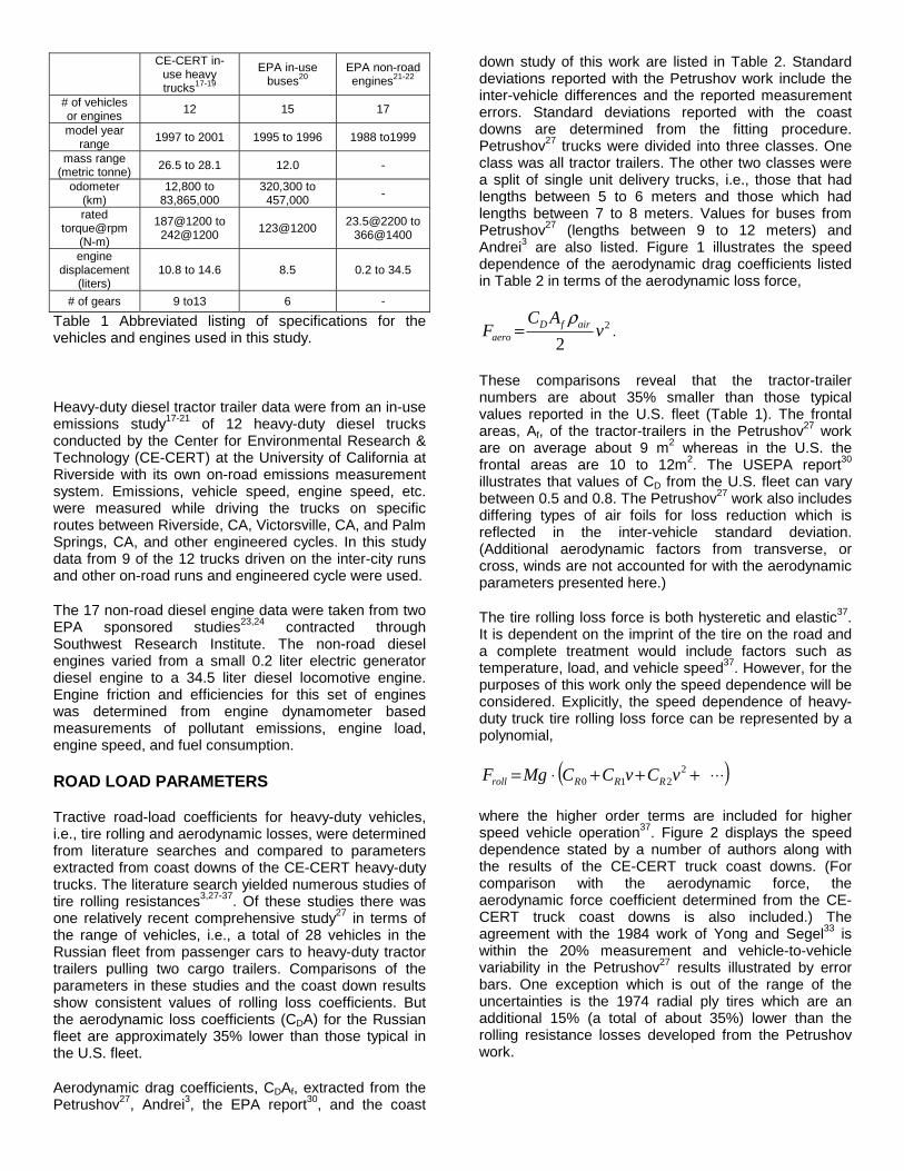
Table 1 Abbreviated listing of specifications for the vehicles and engines used in this study.

Heavy-duty diesel tractor trailer data were from an in-use emissions study17-21 of 12 heavy-duty diesel trucks conducted by the Center for Environmental Research & Technology (CE-CERT) at the University of California at Riverside with its own on-road emissions measurement system. Emissions, vehicle speed, engine speed, etc. were measured while driving the trucks on specific routes between Riverside, CA, Victorsville, CA, and Palm Springs, CA, and other engineered cycles. In this study data from 9 of the 12 trucks driven on the inter-city runs and other on-road runs and engineered cycle were used.

The 17 non-road diesel engine data were taken from two EPA sponsored studies23,24 contracted through Southwest Research Institute. The non-road diesel engines varied from a small 0.2 liter electric generator diesel engine to a 34.5 liter diesel locomotive engine. Engine friction and efficiencies for this set of engines was determined from engine dynamometer based measurements of pollutant emissions, engine load, engine speed, and fuel consumption.

ROAD LOAD PARAMETERS

Tractive road-load coefficients for heavy-duty vehicles, i.e., tire rolling and aerodynamic losses, were determined from literature searches and compared to parameters extracted from coast downs of the CE-CERT heavy-duty trucks. The literature search yielded numerous studies of tire rolling resistances3,27-37. Of these studies there was one relatively recent comprehensive study27 in terms of the range of vehicles, i.e., a total of 28 vehicles in the Russian fleet from passenger cars to heavy-duty tractor trailers pulling two cargo trailers. Comparisons of the parameters in these studies and the coast down results show consistent values of rolling loss coefficients. But the aerodynamic loss coefficients (CDA) for the Russian fleet are approximately 35% lower than those typical in the U.S. fleet.

Aerodynamic drag coefficients, CDAf, extracted from the Petrushov27, Andrei3, the EPA report30, and the coast

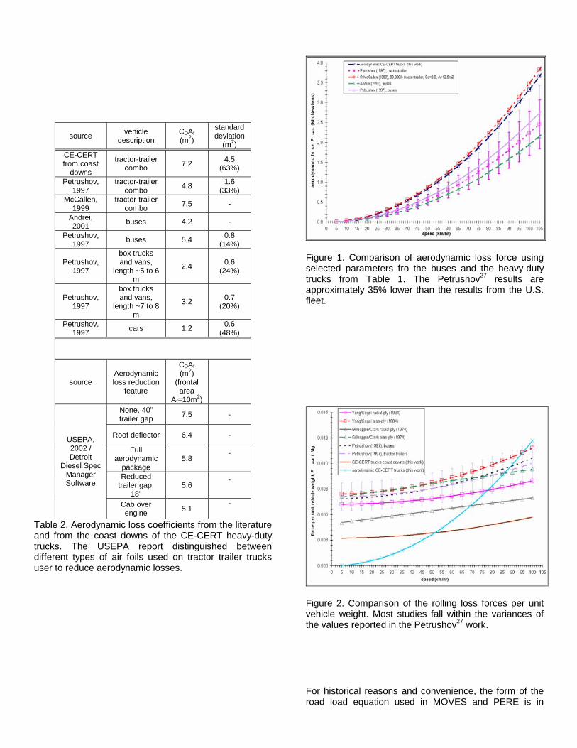
down study of this work are listed in Table 2. Standard deviations reported with the Petrushov work include the inter-vehicle differences and the reported measurement errors. Standard deviations reported with the coast downs are determined from the fitting procedure. Petrushov27 trucks were divided into three classes. One class was all tractor trailers. The other two classes were a split of single unit delivery trucks, i.e., those that had lengths between 5 to 6 meters and those which had lengths between 7 to 8 meters. Values for buses from Petrushov27 (lengths between 9 to 12 meters) and Andrei3 are also listed. Figure 1 illustrates the speed dependence of the aerodynamic drag coefficients listed in Table 2 in terms of the aerodynamic loss force,

2

2v

ACF airfD

aero

ρ= .

These comparisons reveal that the tractor-trailer numbers are about 35% smaller than those typical values reported in the U.S. fleet (Table 1). The frontal areas, Af, of the tractor-trailers in the Petrushov27 work are on average about 9 m2 whereas in the U.S. the frontal areas are 10 to 12m2. The USEPA report30 illustrates that values of CD from the U.S. fleet can vary between 0.5 and 0.8. The Petrushov27 work also includes differing types of air foils for loss reduction which is reflected in the inter-vehicle standard deviation. (Additional aerodynamic factors from transverse, or cross, winds are not accounted for with the aerodynamic parameters presented here.)

The tire rolling loss force is both hysteretic and elastic37. It is dependent on the imprint of the tire on the road and a complete treatment would include factors such as temperature, load, and vehicle speed37. However, for the purposes of this work only the speed dependence will be considered. Explicitly, the speed dependence of heavy-duty truck tire rolling loss force can be represented by a polynomial,

( )⋅⋅⋅+++⋅= 2210 vCvCCMgF RRRroll

where the higher order terms are included for higher speed vehicle operation37. Figure 2 displays the speed dependence stated by a number of authors along with the results of the CE-CERT truck coast downs. (For comparison with the aerodynamic force, the aerodynamic force coefficient determined from the CE-CERT truck coast downs is also included.) The agreement with the 1984 work of Yong and Segel33 is within the 20% measurement and vehicle-to-vehicle variability in the Petrushov27 results illustrated by error bars. One exception which is out of the range of the uncertainties is the 1974 radial ply tires which are an additional 15% (a total of about 35%) lower than the rolling resistance losses developed from the Petrushov work.

source vehicle description

CDAf (m2)

standard deviation

(m2) CE-CERT from coast

downs

tractor-trailer combo 7.2 4.5

(63%)

Petrushov, 1997

tractor-trailer combo 4.8 1.6

(33%) McCallen,

1999 tractor-trailer

combo 7.5 -

Andrei, 2001 buses 4.2 -

Petrushov, 1997 buses 5.4 0.8

(14%)

Petrushov, 1997

box trucks and vans,

length ~5 to 6 m

2.4 0.6 (24%)

Petrushov, 1997

box trucks and vans,

length ~7 to 8 m

3.2 0.7 (20%)

Petrushov, 1997 cars 1.2 0.6

(48%)

source Aerodynamic loss reduction

feature

CDAf (m2)

(frontal area

Af=10m2)

None, 40” trailer gap 7.5 -

Roof deflector 6.4 -

Full aerodynamic

package 5.8

-

Reduced trailer gap,

18” 5.6

-

USEPA, 2002 / Detroit

Diesel Spec Manager Software

Cab over engine 5.1

-

Table 2. Aerodynamic loss coefficients from the literature and from the coast downs of the CE-CERT heavy-duty trucks. The USEPA report distinguished between different types of air foils used on tractor trailer trucks user to reduce aerodynamic losses.

Figure 1. Comparison of aerodynamic loss force using selected parameters fro the buses and the heavy-duty trucks from Table 1. The Petrushov27 results are approximately 35% lower than the results from the U.S. fleet.

Figure 2. Comparison of the rolling loss forces per unit vehicle weight. Most studies fall within the variances of the values reported in the Petrushov27 work.

For historical reasons and convenience, the form of the road load equation used in MOVES and PERE is in

terms of the A, B, and C dynamometer coefficients. Explicitly, the road load force takes the form,

2CvBvAF ++= .

So, assuming for heavy-duty trucks the rolling resistance has a zero and second order dependence on speed, the relationships between the A, B, and C coefficients and the rolling loss and aerodynamic loss coefficients are

MgCAC

C

BMgCA

RairfD

R

2

0

2

.0

+=

==

ρ

where the CR0 and the CR2 are the zero and second order (in speed) rolling resistance force terms.

Dynamometer based emissions testing use empirical A, B, and C tractive road-load parameters which can be related to the rolling resistance and aerodynamic drag coefficients through the speed dependence of the road load equation. Because they are empirically determined they may include additional factors such as axle rotational inertia which can account for approximately 6% of an 18 wheel tractor-trailer’s kinetic energy. (This can be approximated by a simple kinematic analysis of the rotational energy of the truck’s wheels, tires, and axles). Also, additional aerodynamic factors from transverse, or cross, winds are not accounted for with the aerodynamic parameters presented here.

Finally, Table 3 lists the form of the coefficients that are developed from Petrushov as a function of vehicle mass and according to the three heavy-duty truck and the single bus categories described above. The three parameters are listed as the typical road load A, B, and C coefficients. The four different categories are two single unit delivery categories, the tractor-trailer category, and the bus category. The two single unit delivery categories correspond to the two smallest weight categories.

In summary, these tire rolling loss parameters are in reasonable agreement with values from recent literature, but the aerodynamic loss coefficients are lower than what might be expected in the U.S. fleet. The tire rolling losses lie within the variability range of tire rolling losses determined within the last 30 years. The agreement is better for the latter U.S. fleet measurements. The uncertainty in the rolling losses is within 20%. Petrushov25 aerodynamic loss coefficients were found to be lower than the reported values from the U.S. fleet. For example, the values for an 80,000lb tractor-trailers are about 35% lower, with a CD of 0.6 and a frontal area of 12.5 m2 (e.g., McCallen32). The Petrushov27 aerodynamic losses have an uncertainty of about 25% which includes a 5% measurement error along with about a 17% vehicle–to-vehicle variability. MOVES aerodynamic heavy-duty road load coefficients will be updated to

reflect the higher values of aerodynamic losses more typical to the U.S. fleet.

Vehicle classification

A (kW*s/m)

B (kW*s2/m2)

C (kW*s3/m3)

8500 to 14000 lbs (3.855 to

6.350 tonne) 6.22040996.0 M 0

2205

51022.547.1 M−×+

14000 to 33000 lbs (6.350 to 14.968 tonne)

6.22040875.0 M 0

2205

51090.593.1 M−×+

>33000 lbs (>14.968

tonne) 6.22040661.0 M 0

2205

51021.489.2 M−×+

Buses 6.2204

0643.0 M 0 2205

51006.522.3 M−×+

Table 3. A, B, anc C road load parameters developed from Petrushov.

ENGINE PARAMETERS

A Willans line methodology7-15 is used to determine both the engine efficiency and the engine friction of the heavy-duty diesel engines studied in this report. To construct the Willans line for these engines, instantaneous values of fuel mep and bmep were determined from measurements of fuel flow, engine speed, and engine load. The non-road engine measurements23,24 were made on an engine dynamometer. The measurements for the CE-CERT truck17-21 and the AATA bus measurements20 were made with portable emissions measurement systems which recorded engine control module (ECM) , emissions, and the Global Positioning System (GPS) data. This section describes the use of these in-use data to determine engine efficiency and friction using an extension of the Willans methodology first developed by An and Ross7.

Data from the non-road engine study, AATA buses and the CE-CERT trucks had fuel flow measurements from which the fuel mean effective pressure could be determined:

fuel mep = nR*(1000/100)[bar/MPa]*FR*LHV/VdN

where the fuel rate, FR, has units of kg/s, the diesel fuel lower heating value, LHV=43MJ/kg, engine speed, N, is in units of rev/s, the engine displacement, Vd, is in units of m3, and nR is 2 for four stroke engines. The factor of 1000/100 is a conversion factor from MPa to bar as indicated within the boxed parentheses.

Brake mean effective pressure or bmep is determined from engine torque and engine speed measurements for the non-road engines. For both the buses and the CE-CERT trucks, the bmep is determined from manufacturer

engine maximum load curves, engine speed (N), and engine percent load measurements taken from the engine control module (ECM). From the above quantities and the engine displacement, the bmep is calculated as follows,

( )NVNPloadbmep

d

max

100% ×⎟

⎠⎞

⎜⎝⎛=

where % load is the measured percent of the maximum engine load, Vd is the engine displacement, N is the measured engine speed, and Pmax(N) is the maximum engine load (and includes volumetric efficiency22).

Figures 3 and 4 illustrate typical fuel mep vs. bmep curves for all of the non-road engine dynamometer based measurements and for the CE-CERT truck 1 on-road measurements, respectively. The CE-CERT truck plot includes only those points where the vehicle acceleration is greater than zero. Clearly, the on-road measurements illustrate the scatter associated with operation of the engine at many of the possible points of the engine map and indicate that a further refinement or data reduction will be needed to determine an accurate engine speed-engine friction relationship. The non-road engines, operated on a dynamometer, are restricted to the constant load operating points.

Table 4 lists the individual non-road engine results for indicated engine efficiency, η, and the fit statistics. The non-road engine efficiencies range between 39% and 46% with an average value of 43% and a standard deviation of about 2%. These engines range in size from 0.2 liters to 34.5 liters (and were from 7 different engine manufacturers). The efficiencies show no indication of a dependence on engine size. Beyond 5L there also appears to be little dependence of engine friction on engine size. Average engine efficiency determined from the on-road road diesel truck measurements is 48% with standard deviation of 2%. Engine efficiency for the AATA buses have a slightly lower average of 46%. Based on this, PERE uses 48% for all heavy-duty on-road diesel applications. Table 5 below lists the values for each of the individual trucks and a single number for all of the buses. Some of the linear fit statistics are included in the table.

A summary of the diesel engine indicated efficiency results are listed in Table 6. The on-road diesel trucks are in agreement with the smaller passenger car results of Wu and Ross10, who looked at four light duty cars with engine sizes ranging from 1 to 2.5 liters. The R2 of the fits are typically at or better than 0.9 and the standard errors in the slope parameter of the linear fits are around 20% of the fit value. The non-road diesel engine efficiencies are typically about 5% lower than the on-road vehicles and the buses are approximately 2% less

efficient than the diesel tractor-trailers which may be due to how the vehicles were driven (including more transients and differing average speeds).

Figure 3. Willans line for non-road dynamometer based measurements of fuel consumption in terms of fuel mean effective (fuel mep) and engine load in terms of brake mean effective pressure (bmep). The slope of this line is the reciprocal of the engine’s indicated efficiency.

Figure 4. Willans line for CE-CERT truck 1 on-road based measurements of fuel consumption (fuel mep) and engine load (bmep) determined from engine maximum load curves and % load measurements. To eliminate idling and braking events, the data were limited to those where the vehicle acceleration was greater than zero.

engine displacement

(liters)

k (bar)

k standard

error (bar) 1/η

1/η standard

error R

2 η

0.2 8.7 0.9 2.43 0.1 0.93 0.42 0.92 5.2 0.4 2.37 0.09 0.83 0.41 2.2 3.4 0.2 2.46 0.05 0.95 0.44 3.9 2.5 0.2 2.25 0.04 0.99 0.46 3.9 3.1 0.5 2.16 0.09 0.95 0.45 4 3.3 0.3 2.22 0.04 0.99 0.41 6 2.3 1.0 2.42 0.1 0.92 0.39

7.4 2.0 0.4 2.55 0.05 0.98 0.45 7.6 3.6 0.3 2.24 0.05 0.99 0.42 8.3 2.4 0.5 2.36 0.06 0.98 0.44 8.8 2.4 0.6 2.29 0.05 0.98 0.43 10 2.3 0.2 2.33 0.02 0.99 0.41

10.1 3.1 0.3 2.44 0.04 0.99 0.46 10.2 2.2 0.4 2.18 0.03 0.998 0.42 10.5 2.5 0.5 2.39 0.06 0.98 0.46 12.7 1.8 0.2 2.17 0.02 0.99 0.44 34.5 2.3 0.2 2.27 0.03 0.99 0.41

Table 4. Values of non-road engine indicated efficiency using the Willans line approach along with R2 and standard errors from the linear fits. Data used for these were from dynamometer based measurements.

engine displacement

(liters) vehicle k (bar) 1/η

standard error in

1/η R2 η

8.5 buses 0.926 2.17 0.01 0.95 0.461 10.8 truck 2 1.81 2.14 0.01 0.92 0.468 11.9 truck 9 1.39 2.21 0.02 0.85 0.452 12.7 truck 6 1.90 1.97 0.03 0.63 0.507 12.7 truck 7 -0.043 2.15 0.02 0.86 0.466 12.7 truck 8 0.611 2.10 0.02 0.83 0.475 12.7 truck 3 -1.10 2.13 0.02 0.83 0.469 14 truck 4 3.91 2.05 0.01 0.95 0.488

14.6 truck 1 4.27 2.10 0.01 0.95 0.476 Table 5. Values of engine indicated efficiency using the Willans line approach with in-use data for the CE-CERT heavy trucks and the EPA AATA buses along with R2 and standard errors from the linear fits.

source average efficiency

standard deviation

(vehicle-to-vehicle

differences)

engine displacement

range

fuel delivery

# of vehicles

or engines

CE-CERT trucks

48% 2%* 10.8 to 14.6 Turbo- EUI 8

AATA buses 46% - 8.5 TDI 15

Non-road

engines 43% 2%* 0.2 to 34.5 varied 17

Wu and Ross**

47% to 49% 1.08 to 2.46 TDI 4

Table 6. Diesel engine indicated efficiencies for buses, heavy-duty trucks and non-road engines. A comparison with the results determined by the earlier work of Wu and Ross10 is also given for comparison.

Next, diesel engine friction dependence on engine speed was determined. Dynamometer based measurements of fuel rate and brake mean effective pressure are done at a single value of engine load and engine speed. On-

road/in-use based measurements don’t yield such ideal conditions. For the on-road measurements shifting, braking, coasting, and idling can yield incorrect engine load – engine speed points. So, to eliminate any of these so-called transient effects, only low acceleration operating modes were included in the Willans lines.

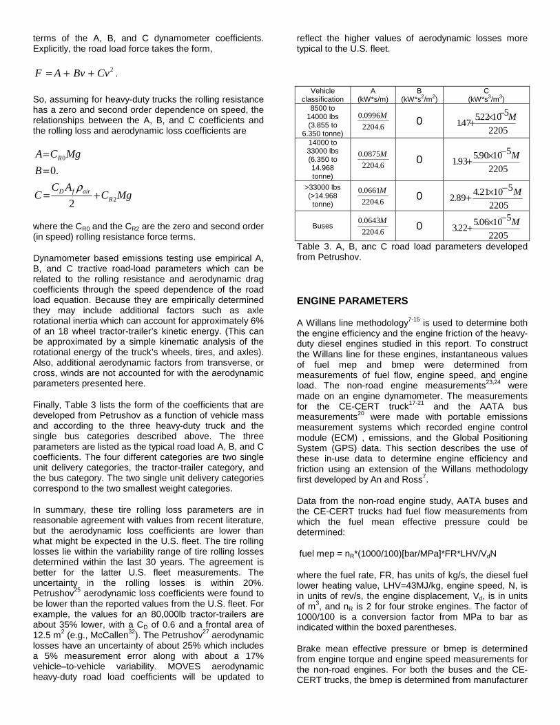
The methodology used to find the frictional losses from in-use data was :

1. a family of fuel mep – bmep graphs were constructed for different values of engine speed (determined by averaging over differing ranges of engine speed); (fuel mep, bmep) points were limited by using positive vehicle accelerations near zero to eliminate transient effects.

2. curve fits were then applied to each of the different graphs, yielding a set of k’s and 1/η’s for a given engine speed (defined by the average engine speed of a range of engine speeds).

3. from these sets of coefficients, the slopes or engine efficiencies, η’s, should be relatively constant, but, the fuel mep-intercepts, k’s, should yield an engine speed dependence which defines the engine friction.

4. finally, fit the fuel mep intercepts (k’s) were fit to a line dependent on engine speed.

Figure 5 and Table 7 illustrate this procedure and show the relatively constant values of engine efficiency as well as the engine speed dependence of engine friction. Except for the lowest engine speed range (mean engine speed = 1045 RPM) the fits had reasonable R2(>0.6). At this lowest engine speed range more than 90% of the points had bmep<4 bar, clustered into two distinct groups, and the points with bmep>4 were relatively scattered.

Final engine friction results together with relative uncertainties (in parentheses) of this study are shown in Table 8 and in Figure 6. (Engine friction results for buses and for the non-road engines were not determinable because of insufficient data.) For comparison, results from Millington and Hartles25,26 and a more recent work (which used the same fuel mep and bmep methodology) by Wu and Ross10 (average the four of their light duty engines). In Figure 6 the uncertainty bars reflect the uncertainties in the engine friction parameters and the engine efficiency determined in this work. Except for higher values of engine speed this work is reasonable agreement with the Wu and Ross work. However, at all engine speeds the Millington and Hartles values range from 30% to 50% higher than the values determined here. At the higher engine speeds, where the differences increase, part of the differences may be due to the inability of this methodology the second order effects of mean piston speed as was done by Millington and Hartles. In general, though, these results may reflect improvements in engine friction which have occurred in the last thirty years.

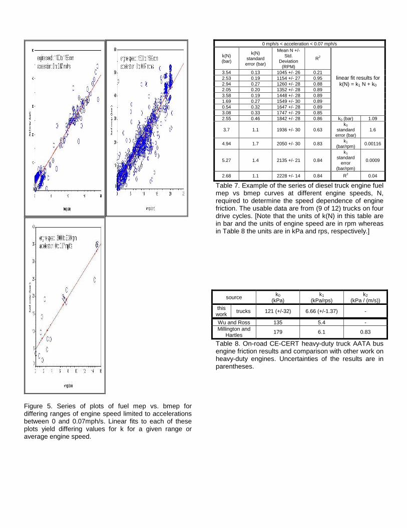
Figure 5. Series of plots of fuel mep vs. bmep for differing ranges of engine speed limited to accelerations between 0 and 0.07mph/s. Linear fits to each of these plots yield differing values for k for a given range or average engine speed.

0 mph/s < acceleration < 0.07 mph/s

k(N) (bar)

k(N) standard

error (bar)

Mean N +/- Std.

Deviation (RPM)

R2

3.54 0.13 1045 +/- 26 0.21 2.53 0.19 1154 +/- 27 0.95 2.94 0.27 1260 +/- 28 0.88 2.05 0.20 1352 +/- 28 0.89 3.58 0.19 1448 +/- 28 0.89 1.69 0.27 1549 +/- 30 0.89 0.54 0.32 1647 +/- 28 0.89 3.08 0.33 1747 +/- 29 0.85

linear fit results for k(N) = k1 N + k0

2.55 0.46 1842 +/- 28 0.86 k0 (bar) 1.09

3.7 1.1 1936 +/- 30 0.63 k0

standard error (bar)

1.6

4.94 1.7 2050 +/- 30 0.83 k1 (bar/rpm) 0.00116

5.27 1.4 2135 +/- 21 0.84

k1 standard

error (bar/rpm)

0.0009

2.68 1.1 2228 +/- 14 0.84 R2 0.04

Table 7. Example of the series of diesel truck engine fuel mep vs bmep curves at different engine speeds, N, required to determine the speed dependence of engine friction. The usable data are from (9 of 12) trucks on four drive cycles. [Note that the units of k(N) in this table are in bar and the units of engine speed are in rpm whereas in Table 8 the units are in kPa and rps, respectively.]

source k0 (kPa)

k1 (kPa/rps)

k2 (kPa / (m/s))

this work trucks 121 (+/-32) 6.66 (+/-1.37) -

Wu and Ross 135 5.4 - Millington and

Hartles 179 6.1 0.83

Table 8. On-road CE-CERT heavy-duty truck AATA bus engine friction results and comparison with other work on heavy-duty engines. Uncertainties of the results are in parentheses.

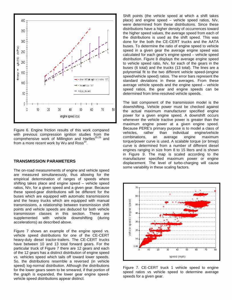
Figure 6. Engine friction results of this work compared with previous compression ignition studies from the comprehensive work of Millington and Hartles25,26 and from a more recent work by Wu and Ross10.

TRANSMISSION PARAMETERS

The on-road measurements of engine and vehicle speed are measured simultaneously, thus allowing for the empirical determination of ranges of speeds where shifting takes place and engine speed – vehicle speed ratios, N/v, for a given speed and a given gear. Because these speed-gear distributions will be different for the buses which are equipped with automatic transmissions and the heavy trucks which are equipped with manual transmissions, a relationship between transmission shift points and vehicle speeds are deduced for both vehicle transmission classes in this section. These are supplemented with vehicle downshifting (during accelerations) as described above.

Figure 7 shows an example of the engine speed vs. vehicle speed distributions for one of the CE-CERT heavy-duty diesel tractor-trailers. The CE-CERT trucks have between 10 and 13 total forward gears. For the particular truck of Figure 7 there are 12 gears and each of the 12 gears has a distinct distribution of engine speed vs. vehicles speed which tails off toward lower speeds. So, the distributions resemble a reversed (in vehicle speed) log-normal distribution. Although the distributions for the lower gears seem to be smeared, if that portion of the graph is expanded, the lower gear engine speed-vehicle speed distributions appear distinct.

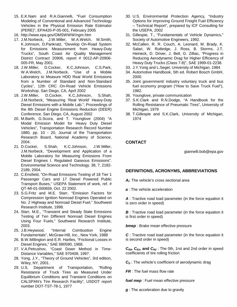
Shift points (the vehicle speed at which a shift takes place) and engine speed – vehicle speed ratios, N/v, were determined from these distributions. Since these distributions have a higher density of occurrences toward the higher speed values, the average speed from each of the distributions is used as the shift speed. This was done for the both the CE-CERT trucks and the AATA buses. To determine the ratio of engine speed to vehicle speed in a given gear the average engine speed was calculated for each gear’s engine speed – vehicle speed distribution. Figure 8 displays the average engine speed to vehicle speed ratio, N/v, for each of the gears in the buses (6 total) and the trucks (13 total). The lines are a polynomial fit to the two different vehicle speed-(engine speed/vehicle speed) ratios. The error bars represent the standard deviations in these averages. From these average vehicle speeds and the engine speed – vehicle speed ratios, the gear and engine speeds can be determined from time-resolved vehicle speeds.

The last component of the transmission model is the downshifting. Vehicle power must be checked against the actual maximum manufacturer specified engine power for a given engine speed. A downshift occurs whenever the vehicle tractive power is greater than the maximum engine power at a given engine speed. Because PERE’s primary purpose is to model a class of vehicles, rather than individual engine/vehicle combinations, an average engine maximum torque/power curve is used. A scalable torque (or bmep) curve is determined from a number of different diesel engines ranging in size from 8 to 15 liters and is shown in Figure 9. The map is scaled according to the manufacturer specified maximum power or engine displacement. The level of turbo-charging will cause some variability in these scaling factors.

Figure 7. CE-CERT truck 1 vehicle speed to engine speed ratios vs vehicle speed to determine average speeds for a given gear.

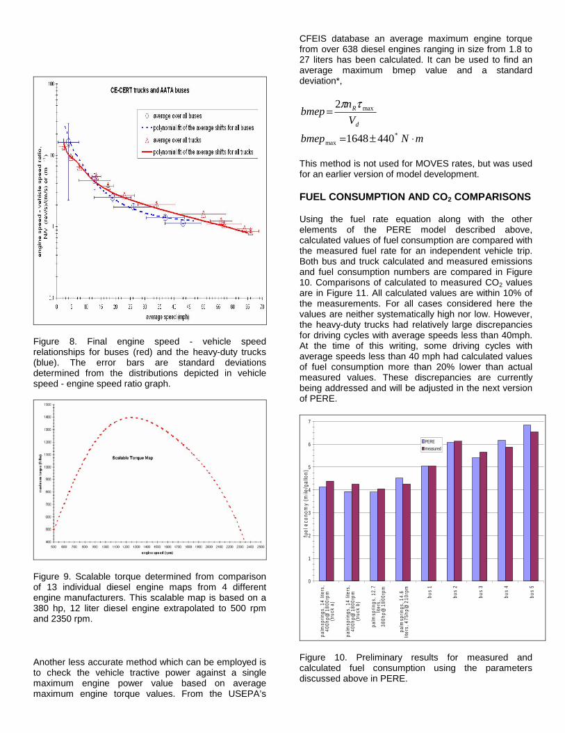
Figure 8. Final engine speed - vehicle speed relationships for buses (red) and the heavy-duty trucks (blue). The error bars are standard deviations determined from the distributions depicted in vehicle speed - engine speed ratio graph.

Figure 9. Scalable torque determined from comparison of 13 individual diesel engine maps from 4 different engine manufacturers. This scalable map is based on a 380 hp, 12 liter diesel engine extrapolated to 500 rpm and 2350 rpm.

Another less accurate method which can be employed is to check the vehicle tractive power against a single maximum engine power value based on average maximum engine torque values. From the USEPA’s

CFEIS database an average maximum engine torque from over 638 diesel engines ranging in size from 1.8 to 27 liters has been calculated. It can be used to find an average maximum bmep value and a standard deviation*,

mNbmep

Vn

bmepd

R

⋅±=

=

*max

max

4401648

2 τπ

This method is not used for MOVES rates, but was used for an earlier version of model development.

FUEL CONSUMPTION AND CO2 COMPARISONS

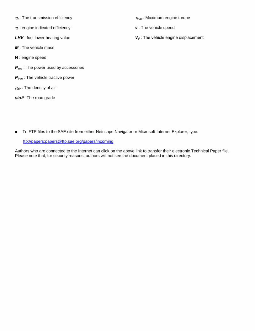
Using the fuel rate equation along with the other elements of the PERE model described above, calculated values of fuel consumption are compared with the measured fuel rate for an independent vehicle trip. Both bus and truck calculated and measured emissions and fuel consumption numbers are compared in Figure 10. Comparisons of calculated to measured CO2 values are in Figure 11. All calculated values are within 10% of the measurements. For all cases considered here the values are neither systematically high nor low. However, the heavy-duty trucks had relatively large discrepancies for driving cycles with average speeds less than 40mph. At the time of this writing, some driving cycles with average speeds less than 40 mph had calculated values of fuel consumption more than 20% lower than actual measured values. These discrepancies are currently being addressed and will be adjusted in the next version of PERE.

0

1

2

3

4

5

6

7

palm

sprin

gs, 1

4 lit

ers,

400h

p@18

00rp

m(tr

uck

a)

palm

sprin

gs, 1

4 lit

ers,

400h

p@18

00rp

m(tr

uck

b)

palm

sprin

gs, 1

2.7

liter

s,38

0hp@

1800

rpm

palm

sprin

gs, 1

4.6

liter

s, 4

75hp

@21

0rpm

bus

1

bus

2

bus

3

bus

4

bus

5

fuel

eco

nom

y (m

ile/g

allo

n)

PEREmeasured

Figure 10. Preliminary results for measured and calculated fuel consumption using the parameters discussed above in PERE.

0

0.5

1

1.5

2

2.5

3pa

lmsp

rings

, 14

liter

s,40

0hp@

1800

rpm

(truc

k b)

palm

sprin

gs, 1

2.7

liter

s,38

0hp@

1800

rpm

(truc

k c)

palm

sprin

gs, 1

4.6

liter

s,47

5hp@

2100

rpm

(truc

k d)

palm

sprin

gs, 1

0.8

liter

s,33

0hp@

1800

rpm

(truc

k e) bu

s 1

bus

2

bus

3

bus

4

bus

5

CO

2 (kg

/mile

)

PEREmeasured

Figure 11. Preliminary results for measured and calculated CO2 using the parameters discussed above in PERE.

CONCLUSIONS

This work demonstrates methodologies for determining engine friction, engine efficiency, and heavy-duty diesel truck and diesel transit bus shift schedules from in-use vehicle measurements. Also, a compilation of bus and heavy-duty diesel truck road load coefficients from a literature search has been given. The heavy truck rolling resistance and aerodynamic coefficients from the literature search have been compared to coast down measurements. The engine efficiencies and friction for 27 heavy-duty diesel vehicles and diesel transit buses were determined with uncertainties of about 20%. Further refinements of the engine speed dependence to reflect pumping losses at higher engine speeds may be needed. Road load parameters for heavy-duty vehicles have been determined for a non-U.S. fleet. So, improvements are needed for vehicle size, possibly first order in speed rolling resistance, and rotational inertia. These parameters have been used in PERE and are within 10% of measured values of fuel consumption and CO2 for differing vehicles on individual vehicle trips.

ACKNOWLEDGMENTS

The authors would like to acknowledge the people involved in the testing and data handling portion of this project: Wayne Miller, Kent Johnson, and Chan-Seung Park. Also, the authors would like to acknowledge discussions of this work with MOVES analysis team members : Dave Brzezinski, Edward Glover, Connie Hart, John Koupal, Larry Landman, Gene Tierney, and James Warilla. The contents of this paper reflect the

views of the authors and does not necessarily indicate acceptance by the sponsors.

REFERENCES

1. Jimenez-Palacios, J., “Understanding and Quantifying Motor Vehicle Emissions and Vehicle Specific Power and TILDAS Remote Sensing”, Ph.D. thesis, Massachusetts Institute of Technology, February 1999

2. R.Ramamurthy, “Heavy duty Emissions Inventory and Prediction”, Master’s thesis, West Virginia University, 1999

3. P.Andrei, “Real World Heavy-Duty Vehicle Emissions Modeling”, Master’s thesis, West Virginia University, 2001

4. C.Frey, “Methodology for Developing Modal Emission Rates for EPA’s Multi-Scale Motor Vehicle and Equipment Emission System”, EPA420-R-02-027 October 2002 (Prepared for EPA by Computational Laboratory for Energy, Air, and Risk Department of Civil Engineering North Carolina State University Raleigh, NC EPA Contract No. PR-CI-02-10493)

5. C.Hart, J.Koupal, R.A.Giannelli, “EPA’s Onboard Analysis Shootout: Overview and Results”, EPA420-R-02-026, October 2002

6. J.Koupal, E.K.Nam, R.A.Giannelli, C.Bailey, “The MOVES Approach to Modal Emission Modeling”, CRC On-Road Vehicle Emission Workshop, March 2004

7. F.An and M.Ross, “A Model of Fuel Economy and Driving Patterns”, SAE 930328, 1993

8. R.W.Goodwin and M.Ross, “Off-Cycle Exhaust Emissions from Modern Passenger Cars with Properly-Functioning Emissions Controls”, SAE 960064, 1996

9. M.Ross, “Fuel Efficiency and the Physics of Automobiles”, Contemporary Physics, vol. 38, number 6, 1997

10. W.Wu and M.Ross, “Modeling of Direct Injection Diesel Engine Fuel Consumption”, SAE 971142, 1997

11. M.Thomas and M.Ross, “Development of Second-by-Second Fuel and Emissions Models Based on an Early 1990s Composite Car”, SAE 971010, 1997

12. M.Barth, F.An, J.Norbeck, and M.Ross, “Modal Emissions Modeling: A Physical Approach”, Transportation Research Record No.1520, pp. 81-88, Transportation Research Board, National Academy of Science.

13. F.An, M.Barth, G.Scora, and M.Ross, “Modeling Enleanment Emissions for Light-Duty Vehicles”, Transportation Research Record No. 1641, pp. 48-57. Transportation Research Board, National Academy of Science, 1998.

14. E.K.Nam, “Proof of Concept Investigation for the Physical Emission Rate Estimator (PERE) to be Used in MOVES”, EPA420-R-03-005, February 2003.

15. E.K.Nam and R.A.Giannelli, “Fuel Consumption Modeling of Conventional and Advanced Technology Vehicles in the Physical Emission Rate Estimator (PERE)”, EPA420-P-05-001, February 2005

16. http://www.epa.gov/OMSWWW/ngm.htm 17. J.M.Norbeck, J.W.Miller, W.A.Welch, M.Smith,

K.Johnson, D.Pankratz, “Develop On-Road System for Emissions Measurement from Heavy-Duty Trucks”, South Coast Air Quality Management District Contract 20906, report # 0012-AP-20906-005-FR, May 2001.

18. J.W.Miller, D.Cocker, K.C.Johnson, C.S.Park, W.A.Welch, J.M.Norbeck, “Use of a Mobile Laboratory to Measure HDD Real World Emissions from a Number of Standard and Non-Standard Cycles”, 12th CRC On-Road Vehicle Emissions Workshop. San Diego, CA, April 2002

19. J.W.Miller, D.Cocker, K.C.Johnson, S.Shah, J.M.Norbeck, “Measuring ‘Real World’ Heavy-Duty Diesel Emissions with a Mobile Lab.”, Proceedings of the 8th Diesel Engine Emissions Reduction (DEER) Conference. San Diego, CA, August 2002

20. M.Barth, G.Scora, and T. Younglove (2004) “A Modal Emission Model for Heavy Duty Diesel Vehicles”, Transportation Research Record Number 1880, pp. 10 - 20, Journal of the Transportation Research Board, National Academy of Science, 2004.

21. D.Cocker, S.Shah, K.C.Johnson, J.W.Miller, J.M.Norbeck, “Development and Application of a Mobile Laboratory for Measuring Emissions From Diesel Engines I. Regulated Gaseous Emissions”. Environmental Science and Technology. 38, 7, 2182-2189, 2004.

22. C.Ensfield, “On-Road Emissions Testing of 18 Tier 1 Passenger Cars and 17 Diesel Powered Public Transport Buses,” USEPA Statement of work, ref. # QT-MI-01-000659, Oct. 22 2002.

23. S.G.Fritz and M.E. Starr, “Emission Factors for Compression Ignition Nonroad Engines Operated on No. 2 Highway and Nonroad Diesel Fuel,” Southwest Research Institute, 1998.

24. Starr, M.E., “Transient and Steady State Emissions Testing of Ten Different Nonroad Diesel Engines Using Four Fuels,” Southwest Research Institute, 2003.

25. J.B.Heywood, “Internal Combustion Engine Fundamentals”, McGraw-Hill, Inc., New York, 1988

26. B.W.Millington and E.R. Hartles, “Frictional Losses in Diesel Engines,” SAE 680590, 1968.

27. V.A.Petrushov, “Coast Down Method in Time-Distance Variables,” SAE 970408, 1997.

28. Yong, J.Y., “Theory of Ground Vehicles”, 3rd edition, Wiley, NY, 2001.

29. U.S. Department of Transportation, ”Rolling Resistance of Truck Tires as Measured Under Equilibrium Conditions and Transient Conditions on CALSPAN’s Tire Research Facility”, USDOT report number DOT-TST-78-1, 1977

30. U.S. Environmental Protection Agency, “Industry Options for Improving Ground Freight Fuel Efficiency – Technical Report”, prepared by ICF Consulting for the USEPA, 2002

31. Gillespie, T., “Fundamentals of Vehicle Dynamics,” Society of Automotive Engineers, 1992.

32. McCallen, R, R. Couch, A. Leonard, M. Brady, K. Salari, W. Rutledge, J. Ross, B. Storms, J.T. Heineck, D. Driver, J. Bell, G. Zilliac, “Progress in Reducing Aerodynamic Drag for Higher Efficiency of Heavy Duty Trucks (Class 7-8)”, SAE 1999-01-2238.

33. J.Y.Yong and L.Segel, University of Michigan, 1984 34. Automotive Handbook, 5th ed. Robert Bosch GmbH,

2000. 35. Joint government/ industry voluntary truck and bus

fuel economy program (“How to Save Truck Fuel”), 1982.

36. Younglove, private communication 37. S.K.Clark and R.N.Dodge, “A Handbook for the

Rolling Resistance of Pneumatic Tires”, University of Michigan, 1979

38. T.Gillespie and S.K.Clark, University of Michigan, 1974

CONTACT

giannelli.bob@epa.gov

DEFINITIONS, ACRONYMS, ABBREVIATIONS

Af: The vehicle’s cross sectional area

a : The vehicle acceleration

A : Tractive road load parameter (in the force equation it is zero order in speed)

B : Tractive road load parameter (in the force equation it is first order in speed)

bmep : Brake mean effective pressure

C : Tractive road load parameter (in the force equation it is second order in speed)

CR0, CR1, and CR2 : The 0th, 1rst and 2nd order in speed coefficients of tire rolling friction

CD : The vehicle’s coefficient of aerodynamic drag

FR : The fuel mass flow rate

fuel mep : Fuel mean effective pressure

g : The acceleration due to gravity

ηt : The transmission efficiency

ηi : engine indicated efficiency

LHV : fuel lower heating value

M : The vehicle mass

N : engine speed

Pacc : The power used by accessories

Ptrac : The vehicle tractive power

ρair : The density of air

sinθ : The road grade

τmax : Maximum engine torque

v : The vehicle speed

Vd : The vehicle engine displacement

To FTP files to the SAE site from either Netscape Navigator or Microsoft Internet Explorer, type:

ftp://papers:papers@ftp.sae.org/papers/incoming Authors who are connected to the Internet can click on the above link to transfer their electronic Technical Paper file. Please note that, for security reasons, authors will not see the document placed in this directory.