LAPPEENRANTA UNIVERSITY OF TECHNOLOGY

Faculty of Technology

Degree Program in Energy Technology

HEAT TRANSFER INSIDE INTERNAL COMBUSTION ENGINE:

MODELLING AND COMPARISON WITH EXPERIMENTAL DATA

Lappeenranta, 13.03.13

0407059 Oleg Spitsov

ABSTRACT

Lappeenranta University of Technology

Faculty of Technology

Degree Programme in Energy Technology

Oleg Spitsov

Heat transfer inside internal combustion engine: modelling and comparison with

experimental data.

Master’s thesis

2013

55 pages, 28 figures, 3 tables

Examiners: Andrey Mityakov, Esa Vakkilainen

Keywords: Heat transfer, internal combustion engine, heat transfer modeling.

The paper is devoted to study specific aspects of heat transfer in the combustion chamber of

compression ignited reciprocating internal combustion engines and possibility to directly

measure the heat flux by means of Gradient Heat Flux Sensors (GHFS). A one – dimensional

single zone model proposed by Kyung Tae Yun et al. and implemented with the aid of Matlab,

was used to obtain approximate picture of heat flux behavior in the combustion chamber with

relation to the crank angle. The model’s numerical output was compared to the experimental

results. The experiment was accomplished by A. Mityakov at four stroke diesel engine Indenor

XL4D. Local heat fluxes on the surface of cylinder head were measured with fast – response,

high – sensitive GHFS. The comparison of numerical data with experimental results has revealed

a small deviation in obtained heat flux values throughout the cycle and different behavior of heat

flux curve after Top Dead Center.

TABLE OF CONTENTS

ABSTRACT .................................................................................................................................... 2

TABLE OF CONTENTS ................................................................................................................ 3

LIST OF SYMBOLS AND ABBREVIATIONS ............................................................................ 4

1. INTRODUCTION .................................................................................................................... 6

2. BACKGROUND ...................................................................................................................... 7

2.1. Cycles of reciprocating internal combustion engines ........................................................... 7

2.1.1. The Otto cycle ................................................................................................................... 8

2.1.2. The Diesel cycle .............................................................................................................. 10

2.1.3. The Trinkler cycle ........................................................................................................... 13

2.2. Heat transfer in the cylinder of internal combustion engine .............................................. 14

2.2.1. Heat flux correlations ..................................................................................................... 16

2.3. Modeling of heat transfer in internal combustion engines ................................................. 24

2.4. Principles of heat flux measurements ................................................................................. 31

2.4.1. Spatial temperature difference method ........................................................................... 31

2.4.2. Wire – wound sensors ..................................................................................................... 32

2.4.3. Transverse Seebeck effect based sensors ........................................................................ 33

2.5. Heat flux measurements in the combustion chamber of IC engines .................................. 36

3. MEASUREMENTS OF THE HEAT FLUX IN COMPRESSION IGNITED ENGINES BY

MEANS OF GRADIENT HEAT FLUX SENSORS .................................................................... 42

4. HEAT TRANSFER MODELING AND COMPARISON WITH EXPERIMENTAL

RESULTS ...................................................................................................................................... 44

4.1. Model description ............................................................................................................... 44

4.2. Discussion of results obtained ............................................................................................ 46

5. CONCLUSION ...................................................................................................................... 49

References ..................................................................................................................................... 51

LIST OF SYMBOLS AND ABBREVIATIONS

a, b, c, m, n – experimental coefficients, parameters, exponents

A – heat transfer surface (m2),

Ap – piston area (m2),

B – cylinder bore (m),

Bo – the Boltzmann number,

Cp – specific heat capacity under constant pressure (J/kg/K),

de – equivalent diameter (m),

F – heat flux distribution factor,

h – heat transfer coeffient (W/m2/K),

k – thermal conductivity (W/m/K),

lc – the length of the connecting rod (m),

mf – fuel mass flow rate (g/hr),

Nu – the Nusselt number,

ql – heat flux on

Q – heat transfer rate (W),

p – chamber gas pressure (Pa),

Pr – the Prandtl number,

ρ – gas density (kg/m3),

r – radial distance from the cylinder axis (m),

Re – the Reynolds number,

Sc – cylinder stroke (m),

Tg – chamber gas temperature (K),

Ts – temperature of surface (K),

Tf – temperature of fluid (K),

TW - temperature of chamber wall (K),

Tp – temperature of the flame (K),

Vp – piston velocity (m/s),

ω – angular rotational speed of the crankshaft (rad/s),

ωg – angular velocity of cylinder gases (rad/s)

Greek symbols:

ε – emmisivity of the object,

σ – the Stefan – Boltzmann constant (W/m2/K),

λ – thermal conductivity (W/m/K),

φ – crank angle (degrees),

µ - dynamic viscosity (kg/m/s),

ν – kinematic viscosity (m2/s),

1. INTRODUCTION

The development of modern engines leads to further forcing of its operation process, thus

causing more thermal stress of theirs main parts, forming the combustion chamber. The design

and, especially, the engine development necessitates conducting of comprehensive and thorough

assessments of quality, reliability and performance of all systems and engine parts, comprising

the piston – cylinder group (further mentioned as “the group”). One reason behind it is that the

parts of the group operate under significantly high temperatures and in chemically active

medium. Secondly, simultaneous impact of thermal and mechanical stresses, which are different

during the cycle due to inconstant gas pressure, has high influence on the cylinders durability.

The heat flux, varying significantly during the cycle and reaching the values up to 106 W/m

2 and

higher, is also irregular through the each surface of the group.

As a result of heat transfer, an intense and unsteady heating of every part of the group occurs.

Temperature level of the piston, exhaust valve, cylinder head, valve seats and other parts may

attain to the limiting values in terms of mechanical properties of structural materials. In some

cases there might be a harmful overheating of details which results in a burnout of piston head,

cracking of the walls of the combustion chamber and other effects that lead to the destruction of

the engine. Thus, special measures to ensure optimum thermal regime of the main parts of the

engine are required for its regular operation.

It is the working medium in the cylinder that results in heating and strain of details, being the

main source of heat. Therefore, a careful evaluation of heat transfer conditions, based not on

integral, but on a local heat flux as function of the angle of rotation of the crankshaft, is needed.

It is safe to say that an interest of researchers to that kind of instrumentations is increasingly

mounting. Commonly applied approach to the problem presents a combination of experimental

measures and theoretical calculations. This is done by use quick-response thermocouples,

measuring the average temperature profile in close proximity to the surface. The feedback of

these quick-response thermocouples is utilized to resolve the equation of heat transfer, where the

boundary conditions are known [1, 3], and calculate temperature gradient and heat flux.

Although, the researchers assure of its high accuracy, the error of the measurement does not

exceed 2%, the method does not seem to be convincing and applicable beyond the experiment.

Also, for the heat flux being a vector quantity, the method is unable to provide complete picture

of what is taking place in the cylinder at the moment.

However, there is an emerging approach to measure the heat flux directly. For that purpose, so-

called heat flux sensors are employed. The main feature of heat flux sensor is that it generates an

electrical signal, which is proportional to the aggregate heat rate applied to the surface of the

sensor.

Basic heat transfer models, diverse heat flux sensors and recent experience of theirs application

in internal combustion engines will be discussed further in the paper.

2. BACKGROUND

The chapter reviews special aspects of heat transfer inside the cylinder of the internal

combustion engine and discusses existing experience concerning its modeling.

The chapter is also intended to provide a vision of principles of heat flux measurements.

Theoretical basics and fundamentals of transverse Seebeck Effect based sensors, description of

design, testing and calibration of Gradient Heat Flux Sensor, as well as its possibilities and

prospects of use are presented.

2.1. Cycles of reciprocating internal combustion engines

As can be seen from its name, an internal combustion engine is a heat engine in which fuel

combustion inside the engine transfers heat to the working medium. In these engines during the

first and second stroke, the working medium is air or a mixture of air and an easily inflammable

liquid or gaseous fuel. During the third stroke, the products of combustion of this liquid or gas

fuel (gasoline, kerosene, solar oil, etc.) represent the working medium. In gas engines, the

working medium is under comparably low pressures and its temperatures are well above the

critical temperature, thus, it allows us to consider the working medium as ideal gas and, thereby,

significantly simplifying the thermodynamic analysis of the cycle.

Internal combustion engines have two important advantages, comparing with other types of heat

engines. Firstly, the fact that a high-temperature heat source is located inside the engine, there is

no need for huge heat transfer surfaces to support heat transfer from a high-temperature source to

the working medium. The advantage allows using of compact designs.

The second advantage of internal combustion engines is a possibility to reach higher thermal

efficiencies. It is well known that the uppermost cycle temperature of the working medium in the

engines, where heat is transferred from external source, is limited by the temperature, which does

not entail structural materials failure. Since the heat is released in the volume of the working

medium itself and is not transferred through the walls, the uppermost value of the continuously

changing temperature of the working medium can considerably exceed this limit. It also worth

keeping in mind, that the cylinder walls and the head of the engine are cooled, thus, causing a

considerable increase in the temperature range of the cycle, and thereby increasing its thermal

efficiency. However, constant cooling is proved to cause a deviation of compression from ideal

isoentropic process.

The core component of any reciprocating engine is the cylinder with a piston connected to an

external work consumer by means of a crank shift. A simple engine’s cylinder has two openings

with valves, through one of which the working medium, air or the fuel-air mixture, is induced

into the cylinder, and through the other valve the working medium is exhausted upon completion

of the cycle.

Three main cycles of internal combustion engines are distinguished: the Otto cycle (combustion

at V = const), the Diesel cycle (combustion at p = const), and the Trinkler cycle (combustion

first at V = const and then at p = const).

2.1.1. The Otto cycle

The schematic diagram of the Otto – cycle – operating engine and the indicator diagram of this

engine are shown in Fig.1.

Fig.1 The Otto cycle.

A piston (I) is placed in a cylinder (II) with an inlet (III) and exhaust (IV) valves. The piston

moving from top dead centre to bottom dead centre (process a-I) creates a rarity inside.

Preliminary prepared combustible mixture of air and vaporized gasoline is injected into the

cylinder after the inlet valve opening. The inlet valve closes when the piston reaches BTC, thus,

terminating a fuel supply.

The piston moving in the opposite direction compresses the mixture and causes a pressure rise

(process 1-2). After the pressure of the fuel mixture is compressed to a certain pressure value,

corresponding to point 2 on the indicator diagram, the fuel mixture is ignited with the aid of

spark plug (V). The process of combustion is assumed to be at constant volume, because the

combustion of the fuel mixture is nearly instantaneous and the piston almost makes no

movement.

Combustion is accompanied by the heat release and heat transfer to the working medium inside

the cylinder. Consequently, its pressure rises to a value, corresponding to point 3 on the indicator

diagram (process 2-3). The pressure boost forces the piston to move again from TDC to BDC

and perform work of expansion which is transferred to an external consumer (process 3-4). After

the piston has reached the BDC, exhaust valve IV opens and the cylinder pressure reduces to a

value somewhat exceeding atmospheric pressure (process 4-5), with a fraction of the gas leaving

the cylinder. The piston then travels again from BDC to TDC, ejecting the remaining part of the

exhaust gas into the atmosphere, followed by initiation of a news cycle.

Thermodynamic analysis of the Otto cycle is performed assuming that, for an amount of fuel

injected being relatively small, it is an ideal closed cycle corresponding to the indicator diagram

below (Fig. 2). However, a real cycle of an internal combustion engine is an open cycle. The

working medium is firstly drawn from outside and then ejected to the atmosphere, when cycle is

completed. Assumptions made also include assuming that working fluid is an air, whose content

remains constant throughout the cycle. And heat is added to (process 2-3) and transferred from

(process 4-1) working medium under constant volume.

Fig. 2. Ideal Otto cycle indicator diagram.

For the processes of compression and expansion occurring in quite short time intervals, the heat

exchange with surroundings is neglected so that the processes can be considered isoentropic with

good approximation, provided that the coolant regime, which has its impact, is adjusted and

managed properly.

Now, let us determine the thermal efficiency of the Otto cycle. Equation below is applied to

estimate the amount of heat transferred to the medium during the process 2-3:

),( 231 TTcq (2.1)

where T2 and T3 are the working medium temperatures corresponding to the beginning and

ending of the heat addition process, respectively, and cν is the heat capacity within that

temperature interval.

The amount of heat exhausted during the process 4 – 1 equals to:

),( 141 TTcq (2.2)

where T2 and T3 are the working medium temperatures corresponding to the beginning and

ending of the heat rejection process, respectively.

Thereby, the thermal efficiency of the Otto cycle can be expressed as following:

,

1

1

1)(

)(1

2

1

2

3

1

4

23

14

T

T

T

T

T

T

TTc

TTc

(2.3)

The ratio 21 /TT for an ideal gas during an adiabatic process is determined:

,)( 1

1

2

2

1 k

T

T

(2.4)

where 1

2

is named compression ratio.

Considering the Poisson’s equations (kk

pp 2211 andkk

pp 4433 ) and taking into

account that v2 = v3, and v4 = v1 we obtain:

,2

3

1

4

T

T

T

T (2.5)

Thus, the thermal efficiency of the Otto cycle becomes equal to:

,1

11

k

(2.6)

According to the equation (2.6) it can be concluded that the thermal efficiency of the Otto cycle

depends only on the compression ratio in the process 1-2. Consequently, from that point of view

it makes sense to increase the compression ratio as high as possible. However, in practice,

operating engines at high compression ratios was proved to be impossible due to the fact that an

increase in temperature and pressure is accompanied with probability of spontaneous ignition of

the fuel mixture happening before the piston attains TDC. This might result in the appearance of

knocking, detonation and destruction of engine components. Thus, the conventional Otto cycle

based engines operate at compression ratio not exceeding 12 [66].

2.1.2. The Diesel cycle

One way to enhance the compression ratio is to compress only pure air not a fuel mixture and

inject the fuel into the engine cylinder when the piston is about to reach the TDC. The Diesel

cycle is based on that principle.

The schematic diagram of the Diesel – cycle operating engine and the indicator diagram are

presented at Fig.3:

Fig. 3 The Diesel cycle.

Similarly to the Otto cycle, the piston travels to the BDC making a rarity inside the cylinder

during the process a – 1, but an atmospheric air instead of fuel mixture is drawn into it. Further

compression is carried out until the air reaches pressure p2. Commonly, Diesel engines operate

with a compression ratio ranging between 15 and 16) [66].

In the beginning of air expansion, the fuel is injected to the cylinder with the aid of special fuel

injection valve. High temperature of compressed air causes the fuel ignition, which burns at

constant pressure following with gas expansion from ν2 to ν3.

After the process of fuel injection is over, further expansion of working fluid follows the

adiabatic curve 3 – 4. When the piston reaches BDC (point 4), the exhaust valve opens reducing

the cylinder pressure to atmospheric at constant volume.

With several assumptions made similar to the Otto process, the Diesel cycle is simplified and

represented with thermodynamically equivalent ideal closed cycle implemented with pure air

(Fig. 4).

Fig. 4. Ideal Diesel cycle indicator diagram.

The ideal Diesel cycle comprises two adiabat (compression and expansion), the isobare, along

which the heat q1 is added to the working medium from high – temperature source, and the

isochore corresponding to the heat q2 rejection to the low – temperature sink.

The thermal efficiency of the Diesel cycle can be also expressed by equation (). When ideal gas

undergoes isobaric expansion, following relation is to consider:

,2

3

2

3

T

T (2.7)

where ρ represents a degree of preliminary expansion.

Using the Clapeyron’s equation and (2.3), we obtain the expression for the thermal efficiency of

the Diesel cycle:

,1

1

111

1

k

k

k

(2.8)

From the derived equation it can be seen that, as well as in the Otto cycle, the higher

compression ratio, the higher thermal efficiency of the Diesel cycle.

The Otto and Diesel cycles can be compared assuming that both have same compression ratio ε

or same highest temperature of the working medium T3 . The initial properties of the working

medium (p1 , v1, T1) are also the same for the two cycles.

In case, the compression ratio equals ε both for the Diesel and Otto cycles, then, it is clear from

Eqs. (2.6) and (2.8), that the thermal efficiency of the Otto cycle is higher than the thermal

efficiency of the Diesel cycle. However, comparison of the thermal efficiencies at the same

compression ratio ε is not entirely correct, since, as was already mentioned above, the advantage

of the Diesel cycle consists in its ability to realize the cycle with higher compression ratios.

On the contrary, a comparison of the thermal efficiencies of the Otto and Diesel cycles operating

at the same highest cycle temperature T3 shows that the thermal efficiency of the Diesel cycle is

advantageous. In particular, this can be seen from the T-s diagram shown in Fig. 5:

Fig. 5. Comparison of ideal Otto and Diesel cycles in T-S diagram.

Process 1 – 2 – 3 – 4 represents the Diesel cycle and process 1 – 2a – 3 – 4 represents the Otto

cycle. For the isochore 2a – 3 (dotted line), corresponding to the fuel combustion under constant

volume in the Otto process, being steeper than isobar 2 – 3 corresponding to the fuel combustion

under constant pressure in the Diesel cycle, although the heat rejection q2 to the low –

temperature sink is the same, the work 21 qqlc produced in the Diesel cycle exceeds the one

in the Otto cycle.

2.1.3. The Trinkler cycle

The mixed or dual combustion Trinkler cycle represents a combination of abovementioned Otto

and Diesel cycles. The engines operating on this cycle feature possession of so – called

forechamber connected to the cylinder by narrow channel. Figure 6 displays an indicator

diagram of the cycle:

Fig. 6. The Trinkler cycle indicator diagram.

In the working cylinder air is compressed adiabatically until it attains a level of compression that

ensures high – temperature ignition of the liquid fuel supplied into the forechamber (process 1-

2). The forechamber is shaped and located so that it contributes much to a better mixing of the

fuel and air, which results in rapid combustion of a fraction of the fuel in the small volume of the

forechamber (process 2-5).

A pressure rise in the forechamber causes propulsion of unburned fuel, air and combustion

products into cylinder. The displacement of the piston in direction to BDC is accompanied by

fuel afterburning at almost constant pressure (process 5-3).

Upon completion of fuel combustion the products of combustion expand further adiabatically

(process 3-4); the exhaust gases are then ejected from the cylinder (process 4-1). Thus, in a dual

combustion engine heat q1, is first added along the isochor (q'1), then following the isobar(q1").

Fig. 7. Comparison of ideal Otto, Diesel and Trinkler cycles in T-S diagram.

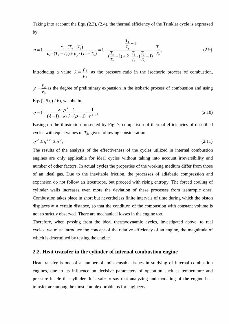
Taking into account the Eqs. (2.3), (2.4), the thermal efficiency of the Trinkler cycle is expressed

by:

,

)1()1(

1

1)()(

)(1

2

1

5

3

2

5

2

5

1

4

5325

14

T

T

T

T

T

Tk

T

T

T

T

TTсTTc

TTc

p

(2.9)

Introducing a value 2

5

p

p as the pressure ratio in the isochoric process of combustion,

5

3

as the degree of preliminary expansion in the isobaric process of combustion and using

Eqs (2.5), (2.6), we obtain:

,1

)1()1(

11

1

k

k

k

(2.10)

Basing on the illustration presented by Fig. 7, comparison of thermal efficiencies of described

cycles with equal values of T3, gives following consideration:

,.. OcdD (2.11)

The results of the analysis of the effectiveness of the cycles utilized in internal combustion

engines are only applicable for ideal cycles without taking into account irreversibility and

number of other factors. In actual cycles the properties of the working medium differ from those

of an ideal gas. Due to the inevitable friction, the processes of adiabatic compression and

expansion do not follow an isoentrope, but proceed with rising entropy. The forced cooling of

cylinder walls increases even more the deviation of these processes from isentropic ones.

Combustion takes place in short but nevertheless finite intervals of time during which the piston

displaces at a certain distance, so that the condition of the combustion with constant volume is

not so strictly observed. There are mechanical losses in the engine too.

Therefore, when passing from the ideal thermodynamic cycles, investigated above, to real

cycles, we must introduce the concept of the relative efficiency of an engine, the magnitude of

which is determined by testing the engine.

2.2. Heat transfer in the cylinder of internal combustion engine

Heat transfer is one of a number of indispensable issues in studying of internal combustion

engines, due to its influence on decisive parameters of operation such as temperature and

pressure inside the cylinder. It is safe to say that analyzing and modeling of the engine heat

transfer are among the most complex problems for engineers.

The heat transfer from combustion gases to the coolant in reciprocating internal combustion

engines varies between 25 – 35% of the total energy released by the mixture of fuel and

combustion air [2]. Nearly half of the heat passes through the cylinder walls and most of the

remaining heat is transferred to the coolant in the cylinder head with the most intensive heat

transfer near the exhaust valve seats.

There are three heat transfer mechanisms: conduction, convection and radiation. Heat transfer by

conduction is an energy transport by means of molecular motion and interaction. Fourier

determined that the heat transfer per unit of area is proportional to the temperature gradient [5]:

,/dx

dTkAQ (2.12)

Heat transfer by convection is an energy transport by means of mass fluid motion. Newton

defined [5] that the heat transfer per area is proportional to the fluid – solid temperature

difference, which basically takes place across a thin layer of fluid close to the solid surface. The

layer is named a boundary layer:

),(/ fs TThAQ (2.13)

Heat transfer by radiation is an energy transport by means of electromagnetic waves from a

surface or a volume, which does not require a heat transfer medium and can take place in

vacuum. The radiation heat transfer is determined to be proportional to the fourth power of the

absolute material temperature [5]:

,/ 4TAQ (2.14)

In the cylinder of the engine heat transfer from the hot combustion gases by conduction and

convection is carried out in the following order: forced convection through the cylinder gas

boundary layer, conduction across the cylinder wall and forced convection through the coolant

liquid boundary layer, where also boiling can occur. Heat transfer by radiation is estimated at

approximately 20 – 40% [2].

The heat transfer process in the cylinder has a periodic nature due to the piston constant

movement. Nevertheless, the engine speed is often high enough to limit the temperature

fluctuations penetrating into the cylinder wall within 0.1 – 0.5 mm deep [7]. Thus, it is assumed

that the cylinder wall has a temperature profile that does not change in time.

Following factors determine a complexity of the heat transfer in the cylinder of internal

combustion engine and are main contributors to extreme unsteadiness and local changes in the

heat transfer:

Turbulence in the cylinder is responsible for typical operating condition of internal

combustion engines, where the Reynolds number is comparably high.

Combustion process affects the heat transfer by rapidly increasing density, pressure and

temperature in the cylinder.

Compression and expansion of the piston has a significant impact on the engine heat

transfer. Firstly, the position of the piston inside the cylinder at the moment of ignition

influences the combustion process. Secondly, the speed of the piston affects the

turbulence.

The abovementioned governing factors are to be understood for successful modeling of the

engine heat transfer.

Heat transfer modeling, as an integral part of numerical studies of internal combustion engines,

is meant to help a manufacturer to enhance the engine performance by accurate prediction of

thermal conditions, to make sure that the conditions doesn’t cause increased emissions, and to

analyze thermal stress limits of cylinder materials.

2.2.1. Heat flux correlations

A number of empirical correlations have been developed to evaluate heat fluxes in the

combustion chambers of internal combustion engines. Some of these expressions are aimed at

calculating of the Nusselt number for forced convection [8, 9]. Other equations are less

theoretical and have been obtained by processing a great body of experimental data [10, 11].

Owing to the complex gas flow in the cylinder, the heat flux does vary in time and location in the

cylinder with changing piston position. The correlations can be grouped, depending on a specific

task they are intended to resolve, or a purpose of calculation. Accordingly, there are correlations

intended to predict the time – averaged heat flux, the instantaneous spatially – averaged heat flux

and the instantaneous local heat fluxes.

The purpose of averaged over time heat flux is to calculate overall steady state energy balance to

predict, for example, the coolant thermal load. Thanks to that approach, component temperatures

and overall heat given by the gases are valid to be estimated. Using the approach the heat

transfer coefficient is expressed in the form of a group of dimensionless numbers [7]:

,RemaNu (2.15)

where Nu, Re denotes dimensionless Nusselt and Reynolds numbers, a, m represent an empiric

coefficient, which are chosen and specific for each engine

Nu and Re numbers are given by:

,

BhNu

,Re

BG (2.16)

where h is defined as a heat transfer coefficient by:

,)( Wgp TTA

Qh

(2.17)

B is a cylinder bore, λ represents gas thermal conductivity, µ - dynamic viscosity and G is the gas

mass rate of flow divided by the piston area Ap.

It is fair to say that accuracy in predicting of heat flux value is determined mainly by selected

empiric parameters.

To describe the relation between heat transfer and crank angle, the instantaneous spatially –

averaged heat flux is studied. It allows predicting, for instance, power output or efficiency,

where the heat flux variation in time is needed. The approach is described in more detail in this

chapter.

Within the instantaneous spatially – averaged heat flux approach, it is assumed that the heat

transfer process inside the cylinder is quasi – steady. It means that at any moment of time the

heat transfer rate can be considered as proportional to the temperature difference between

working fluid and the metal surface. Moreover, a uniformity of the instantaneous gas

temperature distribution in the cylinder is assumed.

The convection heat transfer coefficient depends on different factors and can be calculated by

means of various empirical methods, developed by Nusselt, Woschni, Annand, Hohenberg,

Eichelberg etc.

Heat transfer in reciprocating internal combustion engines was firstly studied by Nusselt.

Processing the experimental results, he derived a formula for the heat – transfer coefficient in the

cylinder of the reciprocating engine [7, 10]:

,

)100

()100

(

421,0)24,11(10388,5

44

3/23/14

Wg

Wg

gpTT

TT

pTVh

(2.18)

Where Tg , p – current values of temperature and pressure of working medium; TW – the chamber

surface temperature.

Obviously, the formula has the additive structure:

,0 RK hhhh (2.19)

where h0 - heat transfer coefficient corresponding to a stationary gas in the combustion chamber,

hK - heat transfer coefficient corresponding to conditions of forced convection at a rate

proportional to the average speed of the piston – Vp, hR - coefficient of heat transfer by radiation.

It should be noted that the dimensional form of the formula reduces the possibility of its

extrapolation to the experimental conditions different from the ones established by Nusselt.

However, he proposed a formally additive approach to the complex, radiation - convective heat

transfer.

Method developed by Nusselt was expanded by his follower in this direction N. Briling.

Conducting experiments to determine the heat loss in a low – speed diesel engine, he found that

intense swirl formation caused by pneumatic spraying of the fuel, increases heat transfer

coefficient of 2.5 times [7, 13]. The formula is represented below:

,

)100

()100

(

421,0)185,045,11(10388,5

44

3/24

Wg

Wg

gpTT

TT

pTVh

(2.20)

The item ,45,1 3/2pTg according to the researcher, is related to the swirl – induced component

of the heat transfer. Further different values of the item were developed for every certain type of

the engine.

The contribution of Russian explorer is that he showed that in every specific case, depending on

the type of fuel mixing, engine speed and power, empiric coefficients should be corrected.

Eichelberg was the first who argued additive approach suggested by Nusselt. Applying noval

method, he deduced the formula below [11]:

,)(109,77 2/14

pg VpTh (2.21)

),()(109,77 2/14

Wgpg TTVpTA

Q (2.22)

The formula features higher meaning of the temperature comparably to the pressure, and an

absence of empiric component of radiation. Thanks to Eichelberg, it was understood that using

of the additive approach to estimate overall heat transfer is inadmissible due to a high share of

heat transfer by radiation in the combustion chamber of a reciprocating compression ignited

engine. The Eichelberg version contains an implicit term for radiation and still is dimensionally

consistent. Therefore, a careful use of units is necessary.

Invesigations of L. Belinsky [7, 14] represent the first and most carefully carried out experiment

on optical measuring of the radiation heat transfer in the chamber of the reciprocating engine. He

established that the radiation in the combustion chamber as a whole is solid, thus, micro particles

of soot were proved to be emitters of radiation which is similar to the radiation emitted by solid

body. Finally, the temperature of soot particles differs from the temperature of the working

medium. This temperature is named temperature of flame and is proposed to be defined from the

empirical dependence:

),)2(106.0(exp 24.0BoTT gp (2.23)

The assumption is also used by G. Rozenblit [7, 15], who derived the formula for heat transfer

coefficient:

,)1()()/(

44

02

2/12/1

1

Wp

Wp

u

vspu

TT

TT

c

WaCcBсСh

(2.24)

Where 2/1)( gTRka - is the acoustic speed, C1 and C2 are empiric coefficients,

,43.2

p

pk

BnWvs

- is a speed of sound vibrations, which is considered as a heat transfer

intensifying factor. The formula takes into account thermal boundary layer by introducing

temperature permeability coefficient 2/1)( pc , determined by thermal characteristics of

the layer. Also a time – dependent item

pindicates nonquasi - steady state.

G. Woschni, a renowned scientist in the field of engine design, has developed a correlation for

calculating the heat transfer coefficient [8]. Similarly to Nusselt, he considered the process to be

quasi – steady:

,)]([12793.0 8.0

021

8.053.02.0 ppVP

TVCVCpTDh

rr

rd

pg

(2.25)

The expression contains the values p and Tg, which correspond to the instantaneous conditions

inside the cylinder, working values pr and Tr correspond to a volume Vr of a reference state, for

example beginning of combustion, exhaust valve closure or inlet valve closure. It should be

noted, that the correlation features a presence of two components of velocity of working body

inside the cylinder. In addition to the conveying speed caused by piston, the influence of swirling

due to combustion is considered. The value pr is a pressure in the cylinder, when combustion

does not take place. It is determined by running the engine without fuel supply, but, unlikely to

p, does not appear to be a function of crank angle.

Constants C1 and C2 consider gas velocity changes during the cycle. G. Woschni recommended

following values:

p

u

V

сС 417.018.61 - for scavenging period,

p

u

V

сС 308.028.21 - for compression and expansion period,

00324.02 С - for diesel engines with direct injection,

0062.02 С - for diesel engines with separate combustion chambers.

Originally, the flow in the cylinder was likened to a steady flow in pipeline. Diameter of the

pipeline was replaced by the engine bore, the average flow velocity in the pipeline – by an

average speed of the piston, and the working medium in the engine was attributed

thermophysical properties of the gas in the pipeline. Thus, for the calculation of unsteady heat

transfer in the combustion chamber, Woschni used the theory of similarity. Using empiric

coefficients he considered the complex relationship between the convective and radiation heat

transfer without stating the last as a separate component.

Truth be told, the correlation developed by Woschni has undergone a great deal of criticizing and

generalizing. For instance, Hohenberg [7, 12] discovered that in fast – speed engines with direct

fuel injection in Top Dead Position of the piston a turbulence is rapidly increasing. Accordingly,

the Woschni correlation lacks an accurate estimation of an effect brought by the phenomena.

Hohenberg examined Woschni’s expression and proposed a correlation based on his

experimental observations:

,)( 8.0

2

8.04.006.0

1 CVpTVСh pg

(2.26)

where C1 = 130 and C2 = 1.4.

Hohenberg reflected on the impact of variable volume at gas flow inside the cylinder by bringing

in the formula a variable linear dimension. He proposed to use the diameter of a sphere which

volume corresponds to the instant value of cylinder volume Vφ, which in its turn is a function of

a crank angle.

Thus, Hohenberg, processing experimental results, revealed some improvements and indicated

that in a particular case of fast – speed direct injection engines, Woschni’s correlation is not

sufficiently correct. He has stated that it overestimates the heat transfer coefficient during

compression and underestimates it during combustion, which results in an overall overestimation

of the heat transfer.

Annand [9] suggested another widely used correlation, where the heat transfer coefficient was

represented by:

,)(

)(Re

44

Wg

Wgb

TT

TTc

B

kah

(2.27)

The Annand’s correlation was a result of processing of experimental data in two different

compression ignited engines: one being a two – stroke and the other a four – stroke. As well as in

Nusselt correlation (), properties of gas were taken at the bulk temperature. Recommended

coefficients a, b, c were:

a = 0.25 to 0.8,

b = 0.7,

c = 0.576σ for compression ignition engines.

Interestingly, coefficients b, c don’t differ significantly for both types of engine, however

coefficient a representing a level of convective heat transfer does vary from smaller value for the

four – stroke engine to higher value for the two – stroke one. This variation of parameter a

indicates that significant factors were ignored and presumptions done by Annand were not

accurate enough.

An equation proposed by Sitkei and Ramanaiah [16] was derived by means of Woschni

correlation and also by Annand’s formula. Similarly to Annand’s, the equation features separated

convection and radiation terms. Thus, the authors recognize the significance of radiant heat

transfer in compression ignited engines. The heat transfer coefficient was given by:

,)(

)(10)1(46

44

8

3.02.0

7.07.0

Wg

Wg

eg

p

TT

TT

dT

Vpbh

(2.28)

where parameter b is:

b = 0 to 0.03 – for direct combustion chamber,

b = 0.05 to 0.1 – for piston chamber,

b = 0.15 to 0.25 – for swirl chamber,

b = 0.25 to 0.35 – for pre – combustion chamber.

Sitkei and Ramanaiah also use equivalent diameter de instead of the cylinder bore. Accordingly,

the variable with the crank angle de represents the geometry of the chamber for appropriately and

is given by:

p

eA

Vd

4. (2.29)

Now, some of the most common correlations for instantaneous spatially - averaged heat flux are

reviewed. These correlations display different methods and experimental approaches used to get

the equations. It cannot be a surprise that comparison of the heat fluxes calculated by each of

these approaches have shown a substantial variation [17], which can be explained by the choice

of empiric coefficients, parameters such as gas velocity or fluid properties, and assumptions

made concerning temperatures of a gas and cylinder wall.

Although the empiric approach for estimating the instantaneous heat flux has its limitations

within a certain operation range, from which the correlation is derived, and is also referred to as

a global or zero - dimensional approach [2], which does not consider the flow field and specific

aspects of the boundary layer, the correlations are still in use for heat transfer simulation in

engines. Main reason for that is their simplicity. In following chapter development of more

complex models, including the ones based on a global model, are surveyed.

The fact that global models lack the resolution to analyze radiation in compression ignited

engines and only allow a calculation of the mean values of heat flux transferred by means of

radiation and do not enable to find out which part of the chamber walls is more or less radiated,

necessitates applying so – called zonal models [2].

Although, zonal models, as well as global ones, do not provide any specific information of local

heat transfer and are empiric constants dependent, are meant to provide an accuracy of

evaluating of heat flux surpassing that provided by global models.

Within the zonal model, several separate zones are distinguished. For example, the cylinder can

be divided into unburned and burned zone in two – zone model [2, 18]. Both burned and

unburned zone has its own history of the heat transfer coefficient, and calculation of the heat flux

is done by each zone accordingly.

Morel and Keribar [19] have developed a computer code named IRIS, which has detailed heat

flux models either for convective and radiation mode of the heat transfer. The convective heat

transfer model is premised on an in – cylinder flow model which calculates swirl and turbulence

as a functions of crank angle. According to the model, the cylinder is divided into three flow

regions, differential equations in each for swirl and turbulence being resolved. All in all, a total

of eleven separate in – cylinder surfaces were taken into account with calculation of each

separate heat transfer coefficient:

,Pr2

1 3/2

1

peff CUСh (2.30)

where 2/122 )2( kUUU yzeff is the effective gas velocity. The values Uz, Uy and k, which is

the turbulent kinetic energy, are obtained from a mean flow model and turbulent model

respectively.

Poulos and Heywood [20] tested turbulence effect on a cycle of spark – ignited engine. They

embodied the turbulence effect by calculating the effective gas velocity as:

,]4

)(22[ 2/1

2 tVKkU

p

eff (2.31)

here K stands for kinetic energy of a mean flow, and k – kinetic energy of the turbulence.

For conducting a thermal analysis of engine components in terms of thermal stresses or modeling

of overall engine performance, including high - accuracy modeling of combustion and emission

formation, calculations of local heat fluxes are required.

To evaluate heat fluxes at any specific location in the combustion chamber, knowledge of local

conditions is important. An equation to estimate the instantaneous heat flux on the cylinder head

or piston was proposed by LeFeuvre [21]:

),(PrRe 33.08.0

Wg

g

l TTr

kaq (2.32)

LeFeuvre adopted the value of Re from correlations for friction factors and heat transfer in

rotating flow systems. It is given by:

,Re

2

gwr (2.33)

and coefficient a being found experimentally in the cylinder of a direct – injection, supercharged

diesel engine, and equalling to 0.047. Tg and Tw represent the mass – averaged gas temperature

and the wall surface temperature respectively.

To establish theoretical grounds for his experiments, LeFeuvre applied the boundary level

theory. A boundary layer theory distinguishes two regions inside the engine cylinder that is near

– wall region and core region, where gas properties are assumed to be uniform, and is a powerful

tool for solving the problems of local heat transfer. A main feature of this model is the

assumption that the movement of gas particles in the boundary layer occurs only in one direction

[7]. Thus, models based on the boundary level theory are classified as one – dimensional.

Unlikely to the global and zonal models, within a one – dimensional model [18] the wall heat

flux can be calculated by solving an energy equation of thermal boundary layer instead of using

the heat transfer coefficient.

LeFeuvre examined the behavior of the forced convection heat transfer in the engine and arrived

to a conclusion that the cycle variation in gas pressure has double effect on the boundary layer

and, consequently, on the heat flux. He found that changes in gas pressure entail a change in the

layer thickness due to a change in density, and a transfer of the energy both in and out of the

boundary layer.

Dent and Suliaman [22] conducted an experiment on an air – cooled, direct – injection diesel

engine with three cylinders in line and two valves in each cylinder. They observed that higher

swirl ratios than the ones reported by LeFeuvre, take place in the engine:

),()(023.0 8.0

2

Wrg

gg

l TTwr

r

kq

(2.34)

The equation () is derived from the correlation for turbulent forced convective heat transfer along

a flat plate surface with gas properties being evaluated at the instantaneous gas temperature Tg.

TWr represents measured surface temperature at every location.

Applicability of the equation () is restricted by a need to have measured or estimated value of TWr

and to conduct a motored test of the engine to collect a data on the swirl, although the

researchers state that the local heat flux in the cylinder head and piston crown can be accurately

enough described by the correlation.

A completely empiric expression based on results, obtained from measurements of the

components temperatures and temperature gradients in over than 200 engines, was proposed by

Alcock et al. [23]:

),()()(10 6

a

bn

b

am

p

f

lT

T

p

p

A

mFq (2.35)

To determine the spatial variation of the heat flux in a cylinder of the engine, knowledge of the

value of the specific distribution factor F, which is defined by the combustion chamber geometry

and location whether it is cylinder head or piston crown.

The coefficients m and n differ according to the type of engine:

m = 0.75, n = 0.3 for four – stroke compression – ignited engines.

Finally, multidimensional model, which is an advanced numerical approach to modeling of heat

transfer, gives detailed spatial information about thermal conditions. In multidimensional model,

several governing equations are resolved. These are conservation equations of mass, momentum

and energy.

In recent years, developing numerical techniques and computer capabilities have boosted such

valuable tools for heat transfer calculations, based on multidimensional model, as Computational

Fluid Dynamics (CFD). Some of these models have proved to be capable of providing more

accurate information of the in – cylinder flow and behavior that other simple models [41, 50, 53,

54]. Generally, numerical computational methods contain following components: mathematical

models (equations); discretization procedures; solution algoritms and computer codes.

Jennings and Morel [24] were the ones who furthered the emergence of CFD approach. They

employed the tool to show the influence of the wall temperature on the temperature gradient

adjacent to the wall.

Within the multi – dimensional approaches, three dimensional equations of mass, momentum

and energy conservation are resolved for core regions. Basically, for near – wall regions current

CFD codes utilize either a wall function or a near wall - layer modeling approach to describe the

conditions in heat transfer calculations [2].

To the date, there are commercial packages as Fluent, STAR_CD, KIVA available for simulating

multiphase flow, which solve the unsteady three – dimensional compressible average Navier –

Stokes equations in addition to a k – ε turbulence model.

2.3. Modeling of heat transfer in internal combustion engines

Application of numerical methods to predict the heat transfer in a cylinder of reciprocating

internal combustion engines is a process of high importance, which was recognized from the

earliest stages of theirs development. Modeling of the heat transfer is usually considered as a part

of whole engine simulation [25 – 42] including combustion modeling, emission and soot

formation modeling, fuel spray modeling etc., and can serve as a prerequisite of performance

optimization and design improvement in order to meet nowadays demands added on the engines.

It is generally agreed that, since reciprocating engines are likely to remain a dominant type of

engine for transport and power in the years to come, improving existing and designing new

engines must be accomplished in terms of lowering a consumption of fuel, enhancing an

environment – friendliness and increasing thermal efficiency.

There are two basic types of models that are in use for modeling of the heat transfer:

thermodynamic and multi – dimensional models. The simplest type of thermodynamic models

are zero – dimensional models or global models, which suits for estimating of the general

parameters by use of semi – empiric correlations. Another kind of thermodynamic models is

quasi – dimensional models.

Currently, the researchers tend to move towards more comprehensive and accurate models

describing the performance of the engine, although, in some cases proved to be impractical for

theirs complexity. Multi – dimensional models are increasingly gaining more attention to due to

their ability to compute the gas motion by numerical solving of the differential equations

representing the laws of mass, energy and momentum conservation, thus, providing a greater

deal of precision.

Global approach was employed by R. Ziarati [25] in 1996 to study the delay period and droplet

penetration. Thanks to the developed model, which used the Annand’s correlation (2.30) to

describe the heat transfer in the combustion chamber and was tested against the experimental

results of a direct injection diesel engine (Ricardo, Atlas) for a number of nozzle configuration,

plunger size and engine speeds and loads. Zarati managed to obtain good agreement of cylinder

pressure and temperature with experimental results (Fig.8).

Fig.8 Predicted and experimental heat release.

Machrafi and Cavadiasa [26] investigated an impact of varying inlet temperature, equivalence

ratio and compression ratio on such parameters of the HCCI engines as heat release and ignition

delay by means of single zone approach.

Experimental results indicated that an increase in equivalence ratio, which is affected by ignition

delay, entails an increase of heat release, and lower residual gas emissions and advances in

ignition delay are reached by an increase of compression ratio.

To predict the performance of a compression ignited engine powered by different blends of

diesel and biodiesel and investigate an effect of variable engine speed and compression ratio on

brake power and thermal efficiency, T.K. Gogoi [27] has developed a simulation model based on

thermodynamic single zone approach. To calculate the heat transfer between the gas and

surroundings he used the equation suggested by Annand (2.30). Proposed model allowed finding

out the correlation between increasing brake power of the engine and speed, a speed value, at

which brake power reaches its peak, thermal efficiency and impact of different blends at these

values.

Fig.9 illustrates variation of brake power with speed for two values of compression ratio.

Fig.9 Variation of brake power with engine speed for two different compression ratios.

It can be seen that increase in engine speed entails an increase in brake power only to a certain

extent. The peak of brake power takes place with a particular engine speed, which is

characteristic of fuel and engine itself. The break power peak occurs at lower engine speeds for

blends with higher share of biodiesel.

In its turn, brake thermal efficiency as a function of engine speed is proved to be on a slight

decrease (Fig. 10).

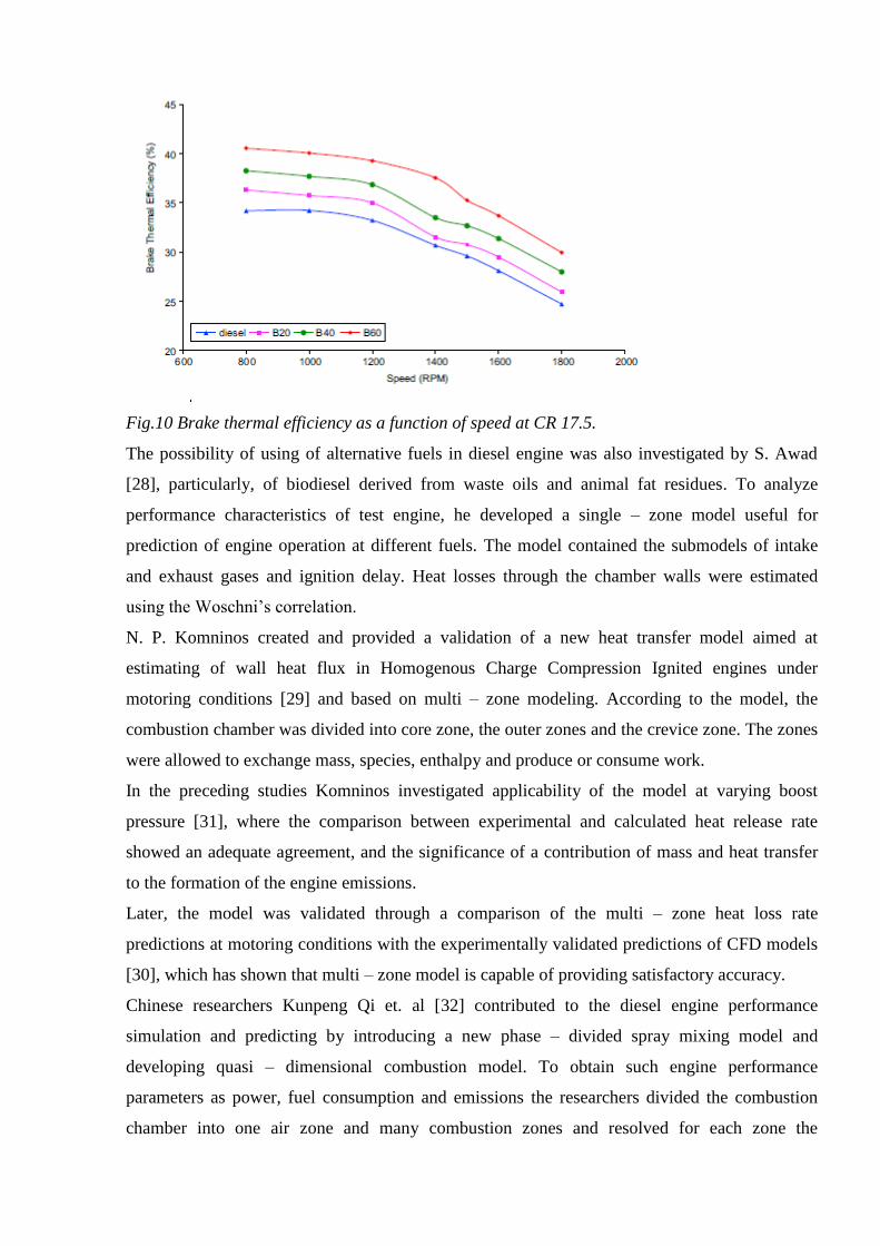
Fig.10 Brake thermal efficiency as a function of speed at CR 17.5.

The possibility of using of alternative fuels in diesel engine was also investigated by S. Awad

[28], particularly, of biodiesel derived from waste oils and animal fat residues. To analyze

performance characteristics of test engine, he developed a single – zone model useful for

prediction of engine operation at different fuels. The model contained the submodels of intake

and exhaust gases and ignition delay. Heat losses through the chamber walls were estimated

using the Woschni’s correlation.

N. P. Komninos created and provided a validation of a new heat transfer model aimed at

estimating of wall heat flux in Homogenous Charge Compression Ignited engines under

motoring conditions [29] and based on multi – zone modeling. According to the model, the

combustion chamber was divided into core zone, the outer zones and the crevice zone. The zones

were allowed to exchange mass, species, enthalpy and produce or consume work.

In the preceding studies Komninos investigated applicability of the model at varying boost

pressure [31], where the comparison between experimental and calculated heat release rate

showed an adequate agreement, and the significance of a contribution of mass and heat transfer

to the formation of the engine emissions.

Later, the model was validated through a comparison of the multi – zone heat loss rate

predictions at motoring conditions with the experimentally validated predictions of CFD models

[30], which has shown that multi – zone model is capable of providing satisfactory accuracy.

Chinese researchers Kunpeng Qi et. al [32] contributed to the diesel engine performance

simulation and predicting by introducing a new phase – divided spray mixing model and

developing quasi – dimensional combustion model. To obtain such engine performance

parameters as power, fuel consumption and emissions the researchers divided the combustion

chamber into one air zone and many combustion zones and resolved for each zone the

combination of energy and mass conservation equations with the ideal state gas equations. The

heat transfer was calculated by use of Brilling’s expression.

The experiment was conducted at 1135 naturally aspirated diesel engine, the results of which

have indicated that the model has sufficient accordance with experimental data.

Z. Sahin and O. Durgun addressed to a quasi – dimensional multi – zone approach to develop a

model, with the aid of which diesel engine cycles and performance parameters were predicted

[33]. The results obtained from simulation were compared to a group of approaches described in

literature.

As in studies of previous authors, the combustion chamber was separated into several zones and

the set of partially – differential equations originated from the first law of thermodynamics, ideal

gas equation and laws of conservation, was resolved. However, to simplify the approach, heat

and mass exchange between zones wasn’t allowed by authors. The heat transfer from the

chamber content to walls was estimated by Annand’s equation.

The prediction results by proposed model revealed accurate enough coincidence with theoretical

calculations, and was further employed by authors to explore performance of diesel engines

using dual fuels and different blends [34], to study heat balance and conduct an energy analysis

[35].

A simulation of porous medium engine by two – zone model considering the heat transfer in

porous medium, the heat transfer from the cylinder wall and mass exchange between zones, was

carried out by Hongsheng Liu et al [36].

The developed model divided the combustion chamber into a cylinder zone, volume of which

changes with time (crank angle), and porous medium zone having a constant volume, each with

different temperatures and mass compositions. The thermodynamic properties are assumed to be

spatially uniform in each zone. To calculate the heat transfer coefficient the correlation proposed

by Woschni was employed.

By means of the model, Hongsheng Liu et al has revealed the significant impact of intake

temperature, initial pressure, compression ratio, excess air ratio, engine speed on the phenomena

of self – ignition and emission formation in a Cummins B – series engine.

Papagiannakis and Hountalas [37] examined the effect of dual fuel operation on the emissions

and performance characteristics of a test diesel engine powered by natural gas as primary fuel

and a pilot amount of diesel fuel for ignition. To estimate combustion duration and intensity,

necessary heat release rate was determined by using the first thermodynamic law and the heat

transfer model of Annand.

Conducted analysis of experimental data has showed that dual fuel combustion process results in

lower peak cylinder temperature and pressure comparing to the conventional diesel. Also a

positive effect of dual fuel combustion on NOx emissions and soot formation has been revealed,

however, a considerable increase in CO and HC level has been discovered.

A study devoted to two – zone modeling of ceramic coated direct injection diesel engines fueled

by blend of conventional diesel and biodiesel was accomplished by B. R. Prasath et at [38].

Developed mathematical model was meant to investigate such combustion and performance

characteristics as cylinder pressure, heat release, heat transfer, specific fuel consumption and

brake thermal efficiency. The properties were calculated on the basis of first law of

thermodynamics and Annand’s equation for gas – wall heat transfer calculations.

To validate predicted considerations, an experiment on a turbocharged diesel engine was carried

out, which resulted in a satisfactory correlation with theoretical results.

Kyung Tae Yun [55] developed a model of reciprocating internal combustion engines to

investigate theirs applicability for combined heat – and – power generation using a one –

dimensional approach. The engine performance and efficiency calculations were coded to create

a user – friendly tool in Visual Basic. Validation of the proposed model was done through

comparison of simulation results with data supplied by engine manufacturer.

The researchers group headed by C. D. Rakopolous [39] contributed much to the heat transfer

modeling. The study published in 1995 presented an advanced two – dimensional multi – zone

model, which was used to investigate and analyze effects of combustion chamber insulation on

the performance and emissions of a direct injection diesel engine.

Basic idea was to divide of the fuel spray into small zones, each of which was considered as an

open system and was allowed exchanging mass and energy with adjacent air zone. The model

included all basic processes occurring in the combustion chamber, and the calculation procedure

integrated the first law of thermodynamics and ideal gas state equations. To estimate the heat

transfer between the gas and the coolant, a zero – dimensional turbulent kinetic energy model K

– ε was employed [2].

Processing experimental data, the authors arrived to the conclusion that since an increase of

exhaust gas enthalpy was observed, it makes sense to take advantage of it in order to improve an

overall efficiency by recovering energy using a power turbine connected to the engine. However,

heat insulation brings a negative impact increasing NOx concentration in exhaust.

Later on, in 2003 Rakopolous [40] created a comprehensive two – zone model, which was

validated against the performance and emissions data results obtained from an experiment on

direct injection compression ignited engine.

Within the model combustion chamber was separated into a non – burning zone of air and a

homogeneous zone, in which fuel was supplied and burned. The mass and energy conservation

equations and perfect gas state equation are employed for each zone. To evaluate the heat

transfer from trapped gas to surroundings, Annand’s correlation was utilized.

In 2009 C. D. Rakopolous et al [41] conducted a research aimed at investigating of effects

caused by varying geometry of the combustion chamber (the ratio of piston bowl diameter to

cylinder diameter was changed from 64% to 54% and 44%) and speed (1500, 2000, 2500 rpm) in

a motored high speed direct injection engine. To do so, Rakopolous used a new quasi –

dimensional engine simulation model, prediction results of which were afterwards validated

against CFD code. Motoring conditions were established to avoid interference of such

parameters as fuel spray penetration, fuel – air mixing process on the in – cylinder temperature

distribution.

The quasi – dimensional model, solving the equation for the conservation of mass and energy by

a finite volume method for the entire cylinder volume, has indicated a good accordance with the

results for mean cylinder pressure predicted by CFD model for all piston ball geometries and

speeds examined. Thus, it was assumed that the model provides enough accuracy at the same

time appearing to be less complex than CFD code.

To simulate fluid flow, heat transfer and combustion process in a single cylinder four – stroke

spark – ignited engine, Mahammadi A. and co – workers [53] have elaborated a CFD code. Near

wall conditions were described by high Reynolds number turbulence model. Turbulent fluxes are

modeled with the aid of k – ε model.

The aim of the study was to estimate a heat flux at different locations inside the chamber: on the

cylinder head, cylinder wall, piston, intake and exhaust valves. The values obtained were

compared with the ones derived from Woschni’s correlation. Relying on the simulation results,

the authors concluded that various places in the cylinder have different values of heat flux with

highest on the intake valve; a maximum pressure has phase difference with maximum

temperature; heat flux reaches its peak value when the pressure is highest.

A notable study, which involved simultaneous experimental and numerical investigating of

thermal processes, performance characteristics and emissions generation, was accomplished by

Rakopolous C. D. et al [50]. The research was performed in a hydrogen – fueled spark – ignited

engine at varying fuel/air and compression ratio. The heat transfer mechanism was investigated

by comparing numerical results obtained from CFD code developed by authors and from

experiment.

The applied in – house CFD code could simulate three – dimensional curvilinear domains by use

of finite volume method. It included the RNG k – ε turbulence model and solved equations for

the conservation of mass, momentum, species and energy [52].

Experimentally measured at different operating conditions parameters were inlet flow rates of air

and hydrogen, the cylinder pressure traces, NOx emissions, inlet and exhaust gas temperatures.

The heat flux was measured at three locations by a Vatell HFM – 7 sensors, three of were

installed at the cylinder liner.

The results obtained indicated that the CFD code is capable to predict accurately enough the heat

transfer in the chamber. It also should be mentioned that slight differences in heat flux values

were observed depending on the measuring locations. The correlation between local heat flux

and crank angle acquired thanks to the experimental data has shown a small displacement of heat

flux peak from the TDC, which probably can be explained by inadequate to the engine speed

sensor’s response time 17 µs [51].

A multi – dimensional CFD model was adopted to study combustion and emission process in

HCCI engine fuelled by dimethyl ether (DME) [54]. Utilization of the STAR – CD commercial

package to simulate an operation of the engine helped to observe a number of features

concerning in – cylinder temperature distribution, high and low temperature reactions separate

locations, content of emissions produced, effect of varying equivalence ratio.

2.4. Principles of heat flux measurements

Heat flux is determined as the amount of heat transferred through the unit of area in a unit of

time and its measurement represents a task of high importance for engineers. Heat flux

measurements are necessary in areas where the measurement of an energy transfer is favoured

over the temperature measurement. Such need can be found in industrial process control or

electrical machines.

In order to measure a heat flux, several basic approaches are developed. Heat flux measurements

are divided into following categories [42]:

A temperature difference is measured over a spatial distance with a certain thermal

resistance;

A temperature difference is measured over time with a known thermal capacitance;

A direct measurement of the energy input or output is made at steady or quasi – steady

conditions. Temperature measurements are conducted to control and oversee the

conditions of the environment;.

A temperature gradient is measured in the medium in close vicinity to the surface.

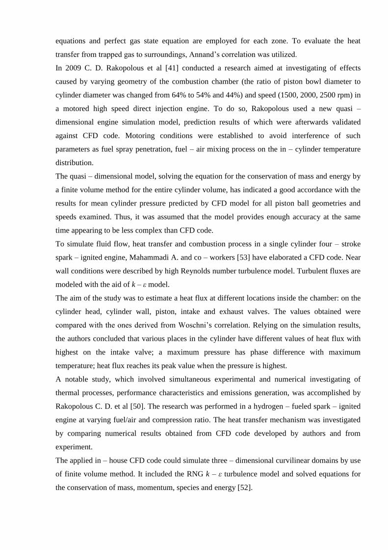
2.4.1. Spatial temperature difference method

To obtain the heat flux, a layered sensor, which sticks to the surface and represents a thermal

resistance layer, is utilized (Fig. 11). With the aid if thermocouples, which is preferable over

resistance temperature detectors, the temperature on either side if the thermal resistance layer is

measured. The thermal gradient is proportional to the heat flux in the direction normal to the

surface. The sensitivity of the sensor is usually enhanced by arranging a thermopile circuit. The

output voltage is derived from the equation:

),( 21 TTSNE t (2.35)

where St is the thermocouple pair Seebeck coefficient.

Fig. 11 . Example of the sensor.

Frankly speaking, the method is not devoid of certain drawbacks. Obviously, a lots of efforts

were done [45 – 49] in order to minimize them.

In the paper [49] Hager describes thin thermopile sensor named Heat Flux Microsensor. He

managed to construct less than 2 - µm thick sensor by using thin – film sputtering techniques.

According to the author, high – temperature material allows the sensor to be used at temperatures

exceeding 800 °C. The thermal response time is estimated around 10 µs.

Also with the aid of sputtering, Van Dorth [45] developed a sensor, which has demonstrated

applicability for measuring of heat fluxes up to 200 kW/m2 and temperatures up to 500 °C.

However, there are still remaining difficulties that concern, firstly, applicability of sensors at

high temperatures and in severe environment. Secondly, accuracy of measurements is not

sufficient due to a relatively lasting response time [44]. Thus, the application for measuring of

heat flux in such rapidly changing processes as a heat transfer in the cylinder of IC engine, is

restricted.

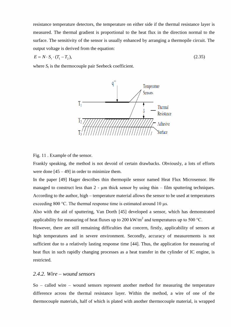
2.4.2. Wire – wound sensors

So – called wire – wound sensors represent another method for measuring the temperature

difference across the thermal resistance layer. Within the method, a wire of one of the

thermocouple materials, half of which is plated with another thermocouple material, is wrapped

around the thermal resistance layer (Fig. 12) [56]. High thermal conductivity materials compose

the thermal resistance layer, while copper plating with constantan wire is a commonly used

combination of materials.

Fig. 12 Schematic wire – wound sensor.

The sensors of that type feature high sensitivity and good time constant around 1 s. However,

measured levels of heat fluxes are limited by 1 kW/m2, normal temperature level is 200 °C [56].

Finally, it was shown by Kidd [57] that the sensors fail to maintain one – dimensional heat

transfer.

2.4.3. Transverse Seebeck effect based sensors

This study deals with heat flux sensors, operation of which is based on the transverse Seebeck

effect. The effect is observed in materials obtaining anisotropy of thermal conductivity, electric

conductivity and thermoelectromotive force. Due to anisotropy in sensors, made of these

materials, the temperature gradients are found in two directions. First one takes place along the

applied heat flux and the second one – across it. The electric field vector E┴ is proportional to the

transversal temperature gradient and is normal to an applied heat flux vector q. In these so –

called gradient heat flux sensors, output signal, proportional to the transversal temperature

gradient, which is proportional to along temperature gradient, which in turn is proportional to an

applied heat flux, is generated [43]. A schematic of the anisotropic thermoelement is shown in

Fig.13

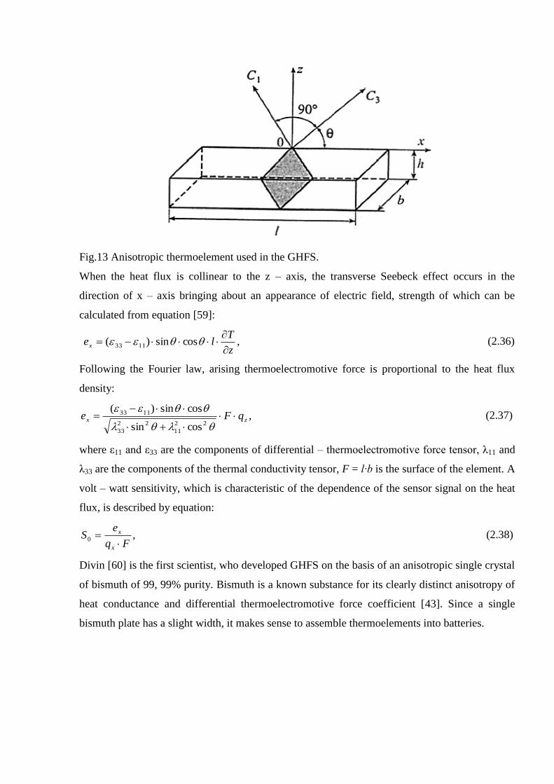
Fig.13 Anisotropic thermoelement used in the GHFS.

When the heat flux is collinear to the z – axis, the transverse Seebeck effect occurs in the

direction of x – axis bringing about an appearance of electric field, strength of which can be

calculated from equation [59]:

,cossin)( 1133z

Tlex

(2.36)

Following the Fourier law, arising thermoelectromotive force is proportional to the heat flux

density:

,cossin

cossin)(

22

11

22

33

1133zx qFe

(2.37)

where ε11 and ε33 are the components of differential – thermoelectromotive force tensor, λ11 and

λ33 are the components of the thermal conductivity tensor, F = l∙b is the surface of the element. A

volt – watt sensitivity, which is characteristic of the dependence of the sensor signal on the heat

flux, is described by equation:

,0Fq

eS

x

x

(2.38)

Divin [60] is the first scientist, who developed GHFS on the basis of an anisotropic single crystal

of bismuth of 99, 99% purity. Bismuth is a known substance for its clearly distinct anisotropy of

heat conductance and differential thermoelectromotive force coefficient [43]. Since a single

bismuth plate has a slight width, it makes sense to assemble thermoelements into batteries.

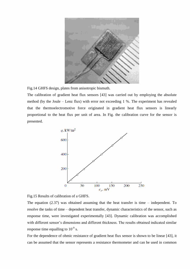
Fig.14 GHFS design, plates from anisotropic bismuth.

The calibration of gradient heat flux sensors [43] was carried out by employing the absolute

method (by the Joule – Lenz flux) with error not exceeding 1 %. The experiment has revealed

that the thermoelectromotive force originated in gradient heat flux sensors is linearly

proportional to the heat flux per unit of area. In Fig. the calibration curve for the sensor is

presented.

Fig.15 Results of calibration of a GHFS.

The equation (2.37) was obtained assuming that the heat transfer is time – independent. To

resolve the tasks of time – dependent heat transfer, dynamic characteristics of the sensor, such as

response time, were investigated experimentally [43]. Dynamic calibration was accomplished

with different sensor’s dimensions and different thickness. The results obtained indicated similar

response time equalling to 10-9

s.

For the dependence of ohmic resistance of gradient heat flux sensor is shown to be linear [43], it

can be assumed that the sensor represents a resistance thermometer and can be used in common

temperature measuring schemes and bridge schemes. The capability of the sensor to generate

electromotive force caused by applied heat flux allows determination of measured temperature

from the equation below with known current and voltage drop in the circuit [59]:

,)1(0 TRR

EI

sh (2.38)

Here I represents current in the circuit, Rsh – shunt resistance, R0 – the sensors resistance under

0°C, χ – coefficient of thermal resistance.

Thus, the use of gradient heat flux sensors provides wider variety of possibilities for collecting

measurement data from experiments and overseeing any thermal process. The GHFS were

utilized to study forced convection and mixed convection on a vertical heated pipe [59, 61], heat

transfer on an even cylindrical surface and on the surface with turbulizers [59], heat transfer in

spherical hole [65], to measure heat flux in the shock tube [59], and showed a good correlation

with theoretical models while proving theirs trustworthiness.

2.5. Heat flux measurements in the combustion chamber of IC engines

For many years, investigations on the heat transfer process in IC engines have been conducted

throughout the world. Diesel engines, spark – ignition engines and homogenous charge

compression – ignition engines fuelled by different fuels such as blends of biodiesel with

traditional diesel fuel, hydrogen, were experimentally studied by researchers.

In addition to simulation and attempts to advance numerical models serving the purpose of

reliable prediction of heat transfer, a lot of experimental efforts were done focusing on

measuring of heat flux at various positions on the cylinder head, liner or piston head. Also there

are recent examples of experiments aiming at investigating of an effect of changing operating

conditions on the heat flux under both motoring and firing mode, thus, providing more thorough

picture of thermal field inside the chamber. There are a number of studies devoted to the

different methods of measuring of heat flux in the chamber of IC engines.

One approach to calculating of the heat flux through a certain location of the combustion

chamber wall is described in the paper [63] and represents a combination of experimental

measures and theoretical calculations and involves measuring of the average temperature profile

in close proximity to the surface with quick – response thermocouples and further determining of

heat flux by means of summing up its stationary and dynamic components.

Assuming the heat flux to be one – dimensional:

2

2

x

T

t

T

, (2.39)

and stating the boundary conditions:

)(),(

)(),0(

TtT

tTtT w , (2.40)

the temperature on the surface was evaluated from:

)sin()cos()(1

tnBtnATtT n

N

n

nww

. (2.41)

An applied equation for heat flux was:

N

n

nnnnww nBAtnBAkTTk

tx

Tktq

1

)sin()()cos()()]()0([),0()(

, (2.42)

where Tw(0), – is the time – averaged surface temperature;

t – current time;

k – thermal conductivity of the material;

An, Bn – amplitude functions defined by the fast Fourier transform;

– shaft speed;

N – number of terms to be summed;

n – number of the current term of the series.

Plots, which illustrate the dependence of measured surface temperature and calculated heat flux

from crank angle, are presented by Fig.16

Fig. 16 Measured surface temperature and calculated heat flux variation with crank angle.

To measure surface temperature Alkidas conducted an experiment at one cylinder of a four –

stroke V – 8 spark – ignition engine with centrally located spark plug. Heat flux probes, each of

which was designed from surface thermocouples and used a second reference thermocouple at a

known depth, were taken from four locations on the cylinder head (Fig. 17).

Fig.17 Location of heat flux probes.

The experimental results have revealed that heat transfer rate reaches its peak after compression

at the beginning of expansion stroke near TDC. Furthermore, the spatial variation of magnitude

of the peak heat flux with position of measurement and sequent order of heat flux increase was

indicated. Fig.18 illustrates typical variations of heat flux measured at four positions with crank

angle for two different engine speeds. Notably, at each engine speed the highest peak heat flux

was measured at the position closest to the centrally located spark plug.

Fig.18 Variations of surface heat flux with crank angle for different engine speed.

Unlikely to the firing conditions, the engine testing in motored conditions did not exhibit the

sequent order of heat flux increase. The increase of heat flux takes place at the same time for all

positions of measurement.

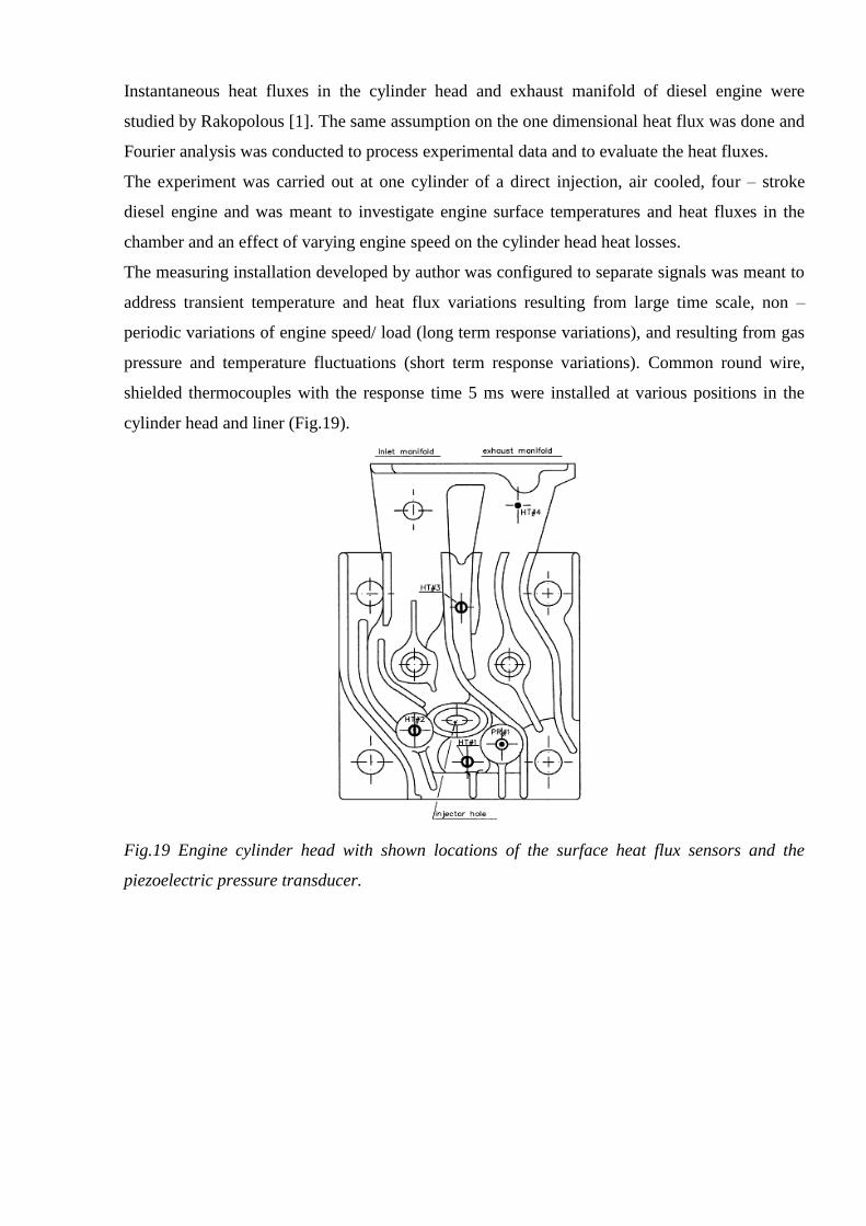
Instantaneous heat fluxes in the cylinder head and exhaust manifold of diesel engine were

studied by Rakopolous [1]. The same assumption on the one dimensional heat flux was done and

Fourier analysis was conducted to process experimental data and to evaluate the heat fluxes.

The experiment was carried out at one cylinder of a direct injection, air cooled, four – stroke

diesel engine and was meant to investigate engine surface temperatures and heat fluxes in the

chamber and an effect of varying engine speed on the cylinder head heat losses.

The measuring installation developed by author was configured to separate signals was meant to

address transient temperature and heat flux variations resulting from large time scale, non –

periodic variations of engine speed/ load (long term response variations), and resulting from gas

pressure and temperature fluctuations (short term response variations). Common round wire,

shielded thermocouples with the response time 5 ms were installed at various positions in the

cylinder head and liner (Fig.19).

Fig.19 Engine cylinder head with shown locations of the surface heat flux sensors and the

piezoelectric pressure transducer.

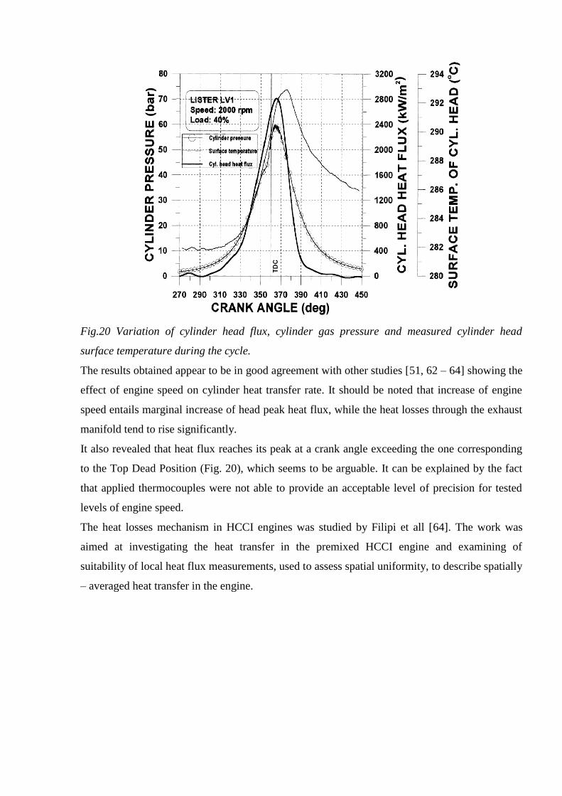
Fig.20 Variation of cylinder head flux, cylinder gas pressure and measured cylinder head

surface temperature during the cycle.

The results obtained appear to be in good agreement with other studies [51, 62 – 64] showing the

effect of engine speed on cylinder heat transfer rate. It should be noted that increase of engine

speed entails marginal increase of head peak heat flux, while the heat losses through the exhaust

manifold tend to rise significantly.

It also revealed that heat flux reaches its peak at a crank angle exceeding the one corresponding

to the Top Dead Position (Fig. 20), which seems to be arguable. It can be explained by the fact

that applied thermocouples were not able to provide an acceptable level of precision for tested

levels of engine speed.

The heat losses mechanism in HCCI engines was studied by Filipi et all [64]. The work was

aimed at investigating the heat transfer in the premixed HCCI engine and examining of

suitability of local heat flux measurements, used to assess spatial uniformity, to describe spatially

– averaged heat transfer in the engine.

Fig. 21 Locations of heat flux probes.

To verify homogeneity of in – cylinder content and uniformity of combustion conditions, the

heat flux measurements were conducted at two positions on cylinder head and seven positions on

piston top (Fig. 21). The coaxial type fast – response thermocouples (1 µs) were installed to

measure instantaneous temperature as a function of crank angle. Assuming one – dimensional

heat flux, stating the boundary conditions and solving the unsteady heat conduction equation

(2.42), the total instantaneous surface heat flux is calculated.

An example of obtained instantaneous temperature and calculated heat flux is presented at Fig.22

Fig. 22 3 – D plots of instantaneous surface side and back side temperature (left) and calculated

heat flux (right).

Another approach to heat flux measurements, which has recently been gaining increasingly more

attention to, concerns various heat flux sensors (HFS). Sensors in the form of a multijunction

differential thermocouple, whose junctions are led out to the opposite sides of a plate from an

insulating material, are very in use. In case the temperatures of the opposite sides are different, a

thermoelectromotive force, whose value is proportional to the temperature difference, is induced.

Importantly, the direction of the thermoelectromotive force coincides with the direction of the

heat flux vector. The effect is usually referred to as the longitudinal Seebeck effect. By use of

such sensors, only the average value of the heat flux can be measured.

A significant part of existing heat flux sensors is capable of operating at a temperature level

about 300 – 500 K. Thus, these sensors cannot be applied for high temperature measurements in

the internal combustion engine due to limiting capability of the materials to stand such severe

ambience. Developing of sliced composites of artificial anisotropic thermoelements

manufactured from metals, alloys or semiconductors has made it possible to get a move on the

new generation of heat flux sensors.

3. MEASUREMENTS OF THE HEAT FLUX IN COMPRESSION

IGNITED ENGINES BY MEANS OF GRADIENT HEAT FLUX

SENSORS

Gradient heat flux sensors appear to have substantial technical potential and attractiveness for

measuring of instantaneous heat fluxes and unsteady heat transfer in the combustion chamber of

CI engines due to its important characteristics such as:

High volt – watt sensitivity,

Fast response matching high speed engines,

Wide range of sensor dimensions and working temperatures.

Use of GHFS helps to obtain data with less errors comparing to the data received by more

commonly applied approach representing a combination of experimental results and following

calculations. Both temperature (when GHFS is employed as thermal resistance) and heat flux can

be measured. The data are transmitted using only one digital channel.

The application of gradient heat flux sensors allowed investigating of instantaneous heat transfer

from the gas to chamber walls. The experiment described in the paper [44] was conducted at four

stroke diesel engine Indenor XL4D. Characteristics of the engine are presented in table (1).

Type Swirl – chamber compression ignited engine

Compression ratio 23

Maximum power 35 kWt (5000 rpm)

Maximum torque 84.3 Nm (2500 rpm)

Cylinder bore 0.125 m

Cylinder stroke 0.180 m

Connecting rod length 0.260 m

Fuel consumption 3.3 m3/h

Table 1 Indenor XL4D characteristics.

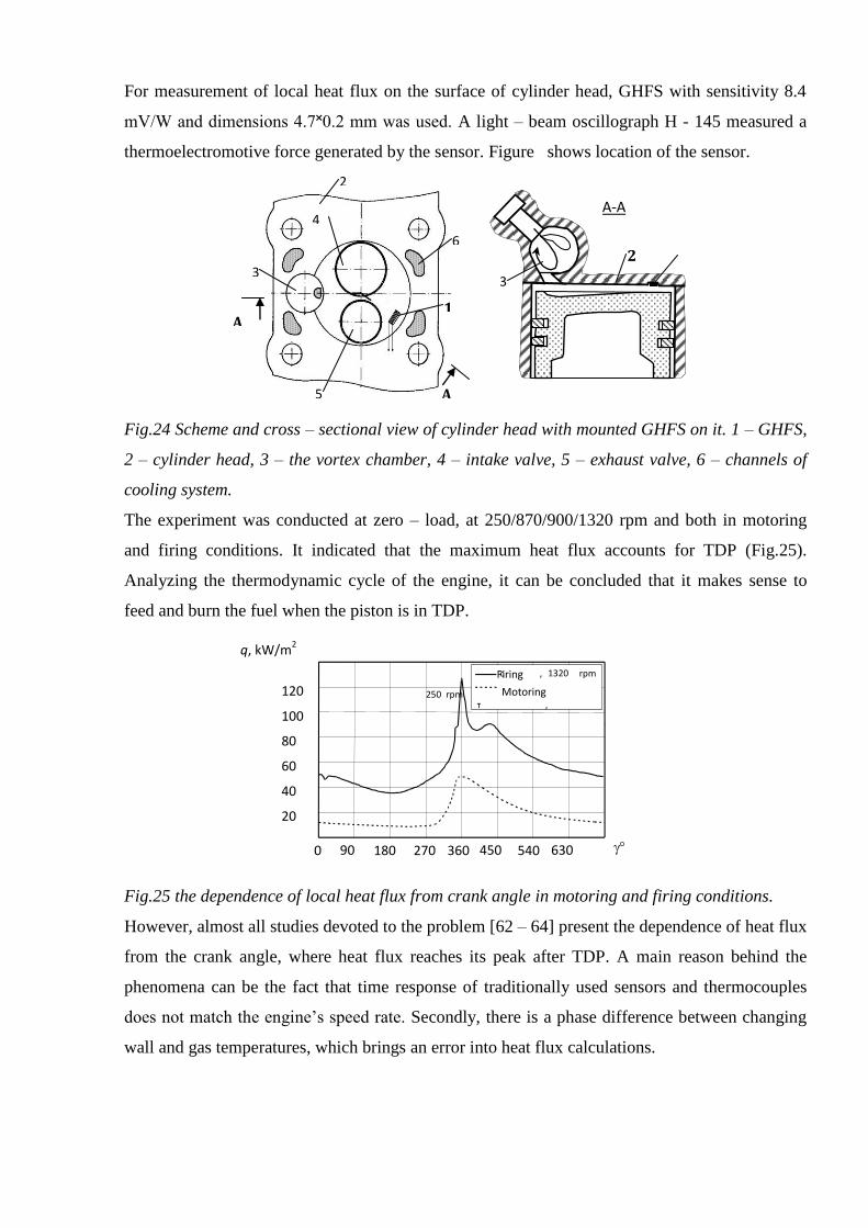
For measurement of local heat flux on the surface of cylinder head, GHFS with sensitivity 8.4

mV/W and dimensions 4.7˟0.2 mm was used. A light – beam oscillograph H - 145 measured a

thermoelectromotive force generated by the sensor. Figure shows location of the sensor.

Fig.24 Scheme and cross – sectional view of cylinder head with mounted GHFS on it. 1 – GHFS,

2 – cylinder head, 3 – the vortex chamber, 4 – intake valve, 5 – exhaust valve, 6 – channels of

cooling system.

The experiment was conducted at zero – load, at 250/870/900/1320 rpm and both in motoring

and firing conditions. It indicated that the maximum heat flux accounts for TDP (Fig.25).

Analyzing the thermodynamic cycle of the engine, it can be concluded that it makes sense to

feed and burn the fuel when the piston is in TDP.

Fig.25 the dependence of local heat flux from crank angle in motoring and firing conditions.

However, almost all studies devoted to the problem [62 – 64] present the dependence of heat flux

from the crank angle, where heat flux reaches its peak after TDP. A main reason behind the

phenomena can be the fact that time response of traditionally used sensors and thermocouples

does not match the engine’s speed rate. Secondly, there is a phase difference between changing

wall and gas temperatures, which brings an error into heat flux calculations.

0 90 180 270 360 450 540 630

20

40

60

80

100

120

с Firing , 1320 rpm Motoring

conditions т , 250 rpm

q, kW/m2

А-А

А

А А

А

1

1

2

2 6

6

4

4 3

3

5

5

3

3

2

2

4. HEAT TRANSFER MODELING AND COMPARISON WITH

EXPERIMENTAL RESULTS

This chapter is devoted to give a description of engine simulation model, developed by Kyung

Tae Yun et al., to present obtained numerical results and to compare with the ones received from

above mentioned experiment.

4.1. Model description

This chapter is devoted to give a description of engine simulation model, developed by Kyung

Tae Yun et al., to present obtained numerical results and to compare with the ones received from

above mentioned experiment.

A thermodynamic model is developed with the aid of Matlab/Simulink based on the engine

model described in the papers [55, 62, 67]. The quasi – one dimensional engine cycle model is

aimed at predicting of transient heat flux during admission, compression, expansion and exhaust

strokes of reciprocating engine.

To determine the transient heat flux inside the chamber, the heat transfer is defined as a function

of crank angle, which is shown in the following equation:

,2

)(

e

wwht

N

TTAh

d

dQ

(4.1)

where T, K – is the mean gas temperature in the cylinder. In present work, the heat transfer

coefficient, h, is determined using Woschni heat transfer correlation:

,26.3 55.02.08.08.0 TBwPh (4.2)

where w is called an average in – cylinder gas velocity, which is calculated during combustion

using the following expression:

),()2( 21 m

oo

od

ce PPVP

TVСsNСw

(4.3)

where Vd is the piston displacement, C1 = 2.28 and C2 = 0.0034 during the combustion and

expansion stroke. However, during the intake, compression and exhaust strokes the average gas

velocity is assumed to be proportional to the mean piston speed.

Histories of pressure and temperature, which are functions of thermodynamic properties,

throughout the cycle are required in order to estimate the average gas velocity. Applying the first

law of thermodynamics expressed in differential form to the content trapped inside the cylinder,

we have:

,)(

i

i

i

htc

vd

dmh

d

dV

V

TRm

d

dQ

d

dQ

d

dmu

d

dTCm

(4.4)

The cylinder geometry represented by the volume as a function of crank angle is derived from:

)],cos(2

))(sin)2

([(2

(1

5.0222

cc

cc

c

c

dd ssll

s

s

V

r

VV (4.5)

Following expression is used to calculate the chemical heat release with the aid of the mass burn

rate:

, d

dxQ

d

dQ b

t

c (4.6)

where Qt is total chemical energy released during the combustion process and equals to:

,fuelfuelt LHVmQ (4.7)

Xb represents mass burned fraction and is expressed on terms of the Wiebe function:

],)(exp[11

wn

d

c

b ax

(4.8)

In equation (4.7), mfuel is the mass of cylinder content during one engine cycle, LHVfuel is lower

heating value of fuel. In equation (4.8), a and nw are Wiebe function parameters, θc is the crank

angle of combustion commencement, θc is duration of combustion process measured in degrees

of crank angle.

Zucrow and Hoffman’s equation [62, 55] is used to define the ratio of specific heats γ for the air

and fuel mixture as a function of temperature. To simplify the equation, a quadratic interpolation

was employed:

,10139.410628.1458.1)( 284 TTT (4.9)

where T – is the cylinder temperature. Following expression describes the specific heat at

constant volume:

,1)(

)(

T

RTс

(4.10)

The specific internal energy and enthalpy can be calculated using:

,1)(

)( dT

T

RTu

(4.11)

,1)(

)()(

dT

T

TRTh

(4.12)

In order to model the intake and exhaust gas exchange process, the equations for gas flow

through a nozzle are used. The mass flow rate is given by:

,])(1[1

2)(

1

/1

ssse

sD

P

P

P

P

RTN

PAC

d

dm (4.13)

For a choked flow:

,

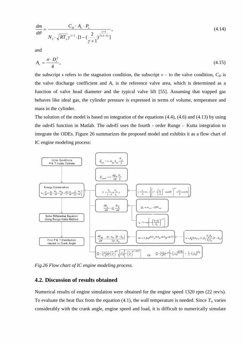
])1

2(1[ )1(2

1

2/1

se

sD

RTN

PAC

d

dm (4.14)

and

,4

2

DA

(4.15)

the subscript s refers to the stagnation condition, the subscript ν – to the valve condition, CD is

the valve discharge coefficient and Aν is the reference valve area, which is determined as a

function of valve head diameter and the typical valve lift [55]. Assuming that trapped gas

behaves like ideal gas, the cylinder pressure is expressed in terms of volume, temperature and

mass in the cylinder.

The solution of the model is based on integration of the equations (4.4), (4.6) and (4.13) by using

the ode45 function in Matlab. The ode45 uses the fourth - order Runge – Kutta integration to

integrate the ODEs. Figure 26 summarizes the proposed model and exhibits it as a flow chart of

IC engine modeling process:

Fig.26 Flow chart of IC engine modeling process.

4.2. Discussion of results obtained

Numerical results of engine simulation were obtained for the engine speed 1320 rpm (22 rev/s).

To evaluate the heat flux from the equation (4.1), the wall temperature is needed. Since Tw varies

considerably with the crank angle, engine speed and load, it is difficult to numerically simulate

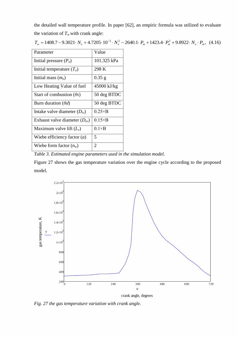
the detailed wall temperature profile. In paper [62], an empiric formula was utilized to evaluate

the variation of Tw with crank angle:

,8922.94.14231.2640107205.43021.97.1408 223

memmeew PNPPNNT (4.16)

Parameter Value

Initial pressure (Po) 101.325 kPa

Initial temperature (To) 298 K

Initial mass (mo) 0.35 g

Low Heating Value of fuel 45000 kJ/kg

Start of combustion (θs) 50 deg BTDC

Burn duration (θd) 50 deg BTDC

Intake valve diameter (Div) 0.25×B

Exhaust valve diameter (Dev) 0.15×B

Maximum valve lift (Lv) 0.1×B

Wiebe efficiency factor (a) 5

Wiebe form factor (nw) 2

Table 3. Estimated engine parameters used in the simulation model.

Figure 27 shows the gas temperature variation over the engine cycle according to the proposed

model.

0 120 240 360 480 600 720200

400

600

800

1 103

1.2 103

1.4 103

1.6 103

1.8 103

2 103

2.2 103

crank angle, degrees

gas

tem

per

ature

, K

T

Fig. 27 the gas temperature variation with crank angle.

Finally, figure 28 shows variation of heat flux over the engine cycle with crank angle. It can be

seen that during the intake stroke the heat flux is slightly increasing. Air compression stroke

features more rapid growth of heat flux with significant jump high to its peak value when

approaching the TDC, so that the most heat energy is generated and transferred to the cylinder

walls, head and piston surface near TDC. During the expansion and exhaust strokes, heat flux is

on a moderate decrease.

0 120 240 360 480 600 7200

40

80

120

160

200

crank angle, degrees

hea

t fl

ux, kW

/m2

qht

Fig.28. Heat flux variation with crank angle.

To evaluate correlations between the measured and predicted values of heat flux, the coefficient

of determination Rd is used:

,)(

)ˆ(

1

2

1

2

n

i i

n

i i

d

yy

yyR (4.17)

where y is the experimental data; y is the mean value of experimental data; and y is the

predicted data. Typicaly, Rd ranges between 0 and 1. The closer is Rd to 1, the better predicted

curve matches experimental results, and vice versa.

According to the heat flux values obtained thanks to simulation model, comparison with the

experiment gives:

7385.0dR .

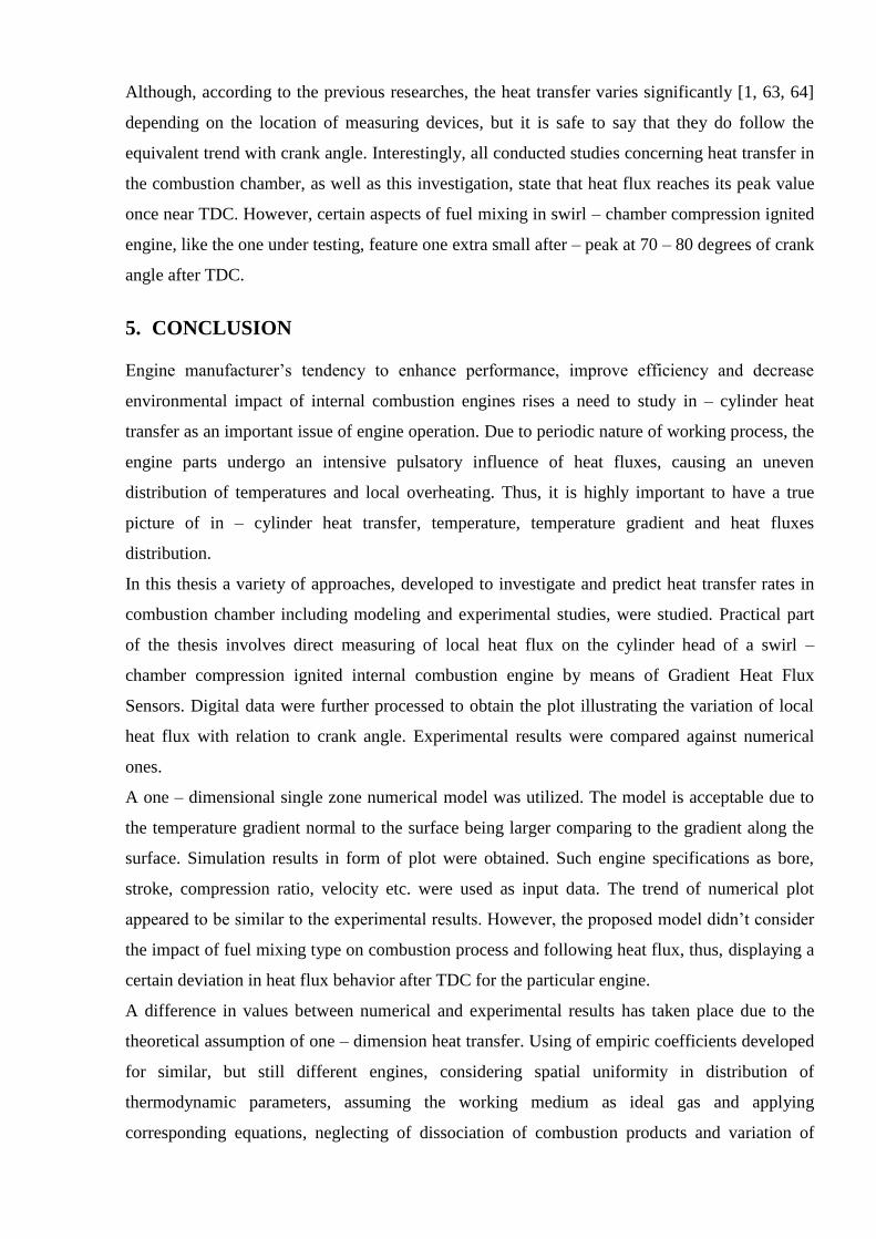
Although, according to the previous researches, the heat transfer varies significantly [1, 63, 64]

depending on the location of measuring devices, but it is safe to say that they do follow the

equivalent trend with crank angle. Interestingly, all conducted studies concerning heat transfer in

the combustion chamber, as well as this investigation, state that heat flux reaches its peak value

once near TDC. However, certain aspects of fuel mixing in swirl – chamber compression ignited

engine, like the one under testing, feature one extra small after – peak at 70 – 80 degrees of crank

angle after TDC.

5. CONCLUSION

Engine manufacturer’s tendency to enhance performance, improve efficiency and decrease

environmental impact of internal combustion engines rises a need to study in – cylinder heat

transfer as an important issue of engine operation. Due to periodic nature of working process, the

engine parts undergo an intensive pulsatory influence of heat fluxes, causing an uneven

distribution of temperatures and local overheating. Thus, it is highly important to have a true

picture of in – cylinder heat transfer, temperature, temperature gradient and heat fluxes

distribution.

In this thesis a variety of approaches, developed to investigate and predict heat transfer rates in

combustion chamber including modeling and experimental studies, were studied. Practical part

of the thesis involves direct measuring of local heat flux on the cylinder head of a swirl –

chamber compression ignited internal combustion engine by means of Gradient Heat Flux

Sensors. Digital data were further processed to obtain the plot illustrating the variation of local

heat flux with relation to crank angle. Experimental results were compared against numerical

ones.

A one – dimensional single zone numerical model was utilized. The model is acceptable due to

the temperature gradient normal to the surface being larger comparing to the gradient along the

surface. Simulation results in form of plot were obtained. Such engine specifications as bore,

stroke, compression ratio, velocity etc. were used as input data. The trend of numerical plot

appeared to be similar to the experimental results. However, the proposed model didn’t consider

the impact of fuel mixing type on combustion process and following heat flux, thus, displaying a

certain deviation in heat flux behavior after TDC for the particular engine.

A difference in values between numerical and experimental results has taken place due to the

theoretical assumption of one – dimension heat transfer. Using of empiric coefficients developed

for similar, but still different engines, considering spatial uniformity in distribution of

thermodynamic parameters, assuming the working medium as ideal gas and applying

corresponding equations, neglecting of dissociation of combustion products and variation of

cylinder mass due to blow – by, are among main contributors as well. Finally, the heat transfer

coefficient was evaluated by Woschni’s expression, application of which to diesel engines a

number of researchers tend to disapprove.

Since the model is not applicable for predicting of heat transfer in motoring conditions, thus, the

comparison with experimental results was done only for firing conditions.

In the experiment a possibility to directly measure heat flux through the engine cylinder head

with calibrated GHFS was demonstrated.

Application – wise, the proposed model is simple enough for analyzing the impact of different

operation characteristics and engine geometry.

References

1. C. D. Rakopolous, G.C. Mavropoulos. 1999. Experimental instantaneous heat fluxes in

the cylinder head and exhaust manifold of an air – cooled diesel engine. Energy

Conversion and Management.

2. Borman G., Nishiwaki K. 1987. Internal – combustion engine heat transfer. Progress in

Energy and Combustion Science.

3. Yuh – Yih Wu, Bo – Chinuan Chen, Feng – Chi Hsieh. 2006. Heat transfer model for

small – scale air – cooled spark – ignition four – stroke engines.

4. Rakesh K. Maurya, Avanish K. Agarwal. 2012. Investigations on the effect of

measurement errors on estimated combustion and performance parameters in HCCI

combustion engine. Measurement.

5. V.P. Isachenko, V.A. Osipova, A.S. Sukomel. 1975. Heat transfer. Moscow, p. 45 – 73,

p. 198 – 243.

6. J.B. Heywood. 1989. Internal combustion engine fundamentals. McGraw – Hill, New –

York, p. 12 – 34, 143 – 197.

7. Kavtaradze R. Z. 2001. Local heat transfer in reciprocating engines. MSTU im.

Baumana.

8. Woschni G. 1967. A universally applicable equation for the instantaneous heat transfer

coefficient in the internal combustion engine. SAE.

9. Annand W. J. D. 1963. Heat transfer in the cylinders of reciprocating internal combustion

engines. Proc. Instn. Mech. Engrs.

10. Nusselt W., 1928. Der Warmeubergang zwischen Arbeitmedium und Zylinderwand in

Kolbenmaschinen. Forachungsarb. Geb. Ing.

11. Eichelberg G.. 1939. Some new investigations on old combustion engine problems.

Engineering.

12. Hohenberg G. F. 1979. Advanced approaches for heat transfer calculations. Society of

automotive engineers, paper № 790825, SAE.

13. Brilling N. R. 1931. Investigating of working process and heat transfer in diesel engine.

Moscow, p. 210 – 256.

14. Belinskiy, L. M. 1955. Heat transfer by radiation in combustion chamber of high – speed

compression ignited engine. Moscow, Mashgiz, p. 145 – 234.

15. Rozenblit, G. B. 1977. Heat transfer in diesel engines. Moscow, p. 32 – 167.

16. Sitkei G., Ramanaiah G. V. 1972. A rational approach for calculation of heat transfer in

diesel engines. Society of automotive engineers.

17. Watson N., Janota, M. S. 1982. Turbocharging the internal combustion engine.

Macmillan education Ltd.

18. Hee Jun Park. 2003. Development of an in – cylinder heat transfer model with variable

density effects on thermal boundary layers. Doctorate dissertation. University of

Michigan.

19. Morel T., Keribar R. 1985. A model for predicting spatially and time – resolved

convective heat transfer in bowl – in – piston combustion chambers. SAE.

20. Poulos S. G., J. B. Heywood. 1983. The effect of chamber geometry on spark ignition

engine combustion. SAE.

21. LeFeuvre T., Myers P. S., Uyehara O. A. 1969. Experimental instantaneous heat fluxes in

a diesel engine and their correlation. Society of automotive engineers, SAE.

22. Dent J. C., Suliaman S. J. 1977. Convective and radiative heat transfer in a high swirl

direct injection diesel engine. Society of automotive engineers, SAE.

23. Alcock J. R., Robson J. V. B., Mash C. 1997. Distribution of heat flow in high duty

internal combustion engines. CIMAC.

24. Jennings M. J., Morel T. 1991. A computational study of wall temperature effects on

engine heat transfer. SAE.

25. Ziarati R. 1990. Mathematical modeling and computer simulation of medium size engine

running on varying quality fuels. International symposium on COMO – DIA.

26. Machrafia H., Cavadiasa S. 2008. An experimental and numerical analysis of the

influence of the inlet temperature, equivalence ratio and compression ratio on the HCCI

auto – ignition process of primary reference fuels in an engine. Fuel processing

technology.

27. Gogoi T. K., Baruah D. C. 2010. A cycle simulation model for predicting the

performance of diesel engine fuelled by diesel and biodiesel blends. Energy.

28. Awad S., Varuel E. G. 2012. Single zone modeling of biodiesel from wastes in diesel

engines. Fuel.

29. Komninos N. P., Kosmadakis G. M. 2010. Heat transfer in HCCI multi – zone modeling:

validation of a new wall heat flux correlation under motoring conditions. Applied energy.

30. Komninos N. P. 2008. Investigating the importance of mass transfer on the formation of

HCCI engine emissions using a multi – zone modeling. Applied energy.

31. Komninos N. P. 2009. Modeling HCCI combustion: modification of a multi – zone

model and comparison to experimental results at varying boost pressure. Applied energy.

32. Kunpeng Qi, Liyan Feng, Xianyin Leng, Baoguo Du, Wuqiang Long. 2010. Simulation

of quasi – dimensional combustion model for predicting diesel engine performance.

Applied mathematical modeling.

33. Sahin Z., Durgun O. 2008. Multi – zone combustion modeling for the prediction of diesel

engine cycles and engine performance parameters. Applied thermal engineering.

34. Sahin Z., Durgun O. 2005. Theoretical investigation of light fuel fumigation and probable

developments in diesel engines. International conference THERMO.

35. Sahin Z., Durgun O. 2007. Theoretical investigation of heat balance in diesel engines.

Energy and environment symposium.

36. Hongscheng Liu, Maozhao Xie, Dan Wu. 2009. Simulation of a porous medium (PM)

engine using a two – zone combustion model. Applied thermal engineering.

37. Papagiannakis R. G., Hountalas D. T. 2004. Combustion and exhaust characteristics of a

dual fuel compression ignition engine operated with pilot diesel fuel and natural gas.

Energy conversion and management.

38. Prasath B. R., Porai P. T., Shabir M. F. 2010. Two – zone modeling of diesel/biodiesel

blended fuel operated ceramic coated direct injection diesel engine. Energy and

environment.

39. Rakopolous C. D., Takus G. N., Tzanos E. I. 2006. Analysis of combustion chamber

insulation effects on the performance and exhaust emissions of a DI diesel engine using a

multi – zone model.

40. Rakopolous C. D., Rakopolous D. C., Giakomis E. G., Kyritsis D. C. 2003. Validation

and sensitivity analysis of a two – zone diesel engine model for combustion and

emissions prediction. Energy conversion and management.

41. Rakopolous C. D., Kosmadakis G. M., Pariotis E. G. 2009. Investigation of piston bowl

geometry and speed effects in a motored HSDI diesel engine using a CFD against a quasi

– dimensional model. Energy conversion and management.

42. Sujay R. – M. 2005. Design and calibration of a novel high temperature heat flux sensor.

Master’s thesis. Virginia Polytechnic University.

43. Mityakov A. V., Sapozhnikov S. Z., Pyrhonen J. 2011. Gradient heat flux sensors for

high temperature environments. Sensors and actuators.

44. Mityakov A. V. 2000. Gradient heat flux sensors for unsteady heat transfer. Doctoral

dissertation. St. Petersburg State Technical University.

45. Van Dorth A. C. 1983. Thick film heat flux sensor. Sensors and Actuators.

46. Hayashi M., Sakurai A., Aso S. 1986. Measurement of heat – transfer coefficients in

shockwave turbulent boundary layer interaction regions with a multi – layered thin film

heat transfer gauge. NASA – TM – 77958.

47. Godefroy J. C., Gageaut C., Francois D., Portat M. 1987. Sputtered alumina layers and

platinel thermocouples for high temperature surface thermometers, evaluations of their

electrical and mechanical characteristics. ONERA TP.

48. Epstein A. H., Guenette G. R., Norton R. J. G., Cao Y. 1986. High frequency response

heat – flux gauge. Rev. Sci. Instrum.

49. Hager J. M., Simmons S., Smith D. 1991. Experimental performance of a heat flux

microsensor. ASME Journal of engineering for gas turbines and power.

50. Rakopolous C. D., Kosmadakis G. M., Demuynck J. 2011. A combined experimental and

numerical study of thermal processes, performance and nitric oxide emissions in a

hydrogen – fueled spark – ignition engine. Hydrogen energy.

51. Demuynck J., Raes N., Zuliani M. 2009. Local heat flux measurements in a hydrogen and

methane spark – ignition engine with a thermopile sensor. Hydrogen energy.

52. Han Z., Reitz R. D. 1995. Turbulence modeling of internal combustion engines using

RNG k – ε models. Combustion Science and Technology.

53. Mohammadi A., Yaghoubi M., Rashidi M. 2007. Analysis of local convective heat

transfer in a spark – ignition engine. International Communications in heat and mass

transfer.

54. Huang Chen, Yao Mingfa, Xingcai Lu. 2008. Study of dimethyl ether homogenous

charge compression ignition combustion process using a multi – dimensional

computational model. International Journal of Thermal Sciences.

55. Kyung Tae Yun, Heejin Cho. 2012. Modeling of reciprocating internal combustion

engines for power generation and heat recovery. Applied energy.

56. Hauser R. L. 1985. Construction and performance of in situ heat flux transducers.

Building Applications of Heat Flux Transducers, pp. 172 – 183.

57. Kidd C. T., Nelson C. G. 2005. How the Schmidt – Boelter sensor really works.

58. A. V. Mityakov, V. Yu. Mityakov, S. Z. Sapozhnikov. 2002. Application of the

transverse Seebeck effect for measurement of instantaneous values of a heat flux on a

vertical heated surface under conditions of free – convection heat transfer. State

Technical University, St. Petersburg.

59. Sapozhnikov S. Z., Mityakov V, Yu., Mityakov A. V. 2006. Gradient heat flux sensors:

possibilities and prospects of use. State Technical University, St. Petersburg.

60. Divin N.P. 1999. Russian Utility Model Certificate no 9959, priority of Aug. 10, 1998,

Byull., Polezn. Model, no. 5.

61. Chumalov Y. S., Nikolskaya S. B.. 1986. Features of dynamic and heat structure of free

convection boundary layer near vertical heated surface, in: Proc. Turbulent Heat transfer

- , Manchester, vol. 2, p.135.

62. Yuh – Yih Wu, Bo – Chiuan Chen, Feng – Chi Hsieh. 2006. Heat transfer for small –

scale air – cooled spark – ignition four – stroke engines. Heat and Mass Transfer.

63. Alkidas A.C. 1980. Heat transfer characteristics of a spark – ignition engine, Trans.

ASME, J Heat transfer.

64. Z. Filipi, J. Chang, D. Assanis. 2004. New heat transfer correlation for an HCCI engine

derived from measurements of instantaneous surface heat flux, Trans SAE, J Engines.

65. S. Z. Sapozhnikov, V. Yu. Mityakov, A. V. Mityakov. 2000. Local heat transfer under

forced convection in spherical hole, in Proc. 4 Minsk Int. Forum on heat and mass

transfer.

66. V.A. Kirillin, V.V. Sychev, A.E. Sheindlin. 1983. Technical Thermodynamics. Moscow,

Energoatomizdat. p.264 – 300.

67. Yusaf T.F., M.Z. Yusoff. 2005. Modeling of transient heat flux in spark ignition engine

during combustion and comparisons with experiment. American Journal of Applied

Sciences, vol. 2, p. 1438 – 1444.