energies

Article

Heat Transfer in a Drilling Fluid withGeothermal Applications

Wei-Tao Wu 1, Nadine Aubry 2, James F. Antaki 1, Mark L. McKoy 3 and Mehrdad Massoudi 4,*1 Department of Biomedical Engineering, Carnegie Mellon University, Pittsburgh, PA 15213, USA;

weitaow@andrew.cmu.edu (W.-T.W.); antaki@andrew.cmu.edu (J.F.A.)2 Department of Mechanical and Industrial Engineering, Northeastern University, Boston, MA 02115, USA;

n.aubry@northeastern.edu3 U.S. Department of Energy, National Energy Technology Laboratory (NETL), 3610 Collins Ferry Road,

Morgantown, WV 26507-0880, USA; mark.mckoy@netl.doe.gov4 U.S. Department of Energy, National Energy Technology Laboratory (NETL), 626 Cochrans Mill Road,

Pittsburgh, PA 15236-0940, USA* Correspondence: mehrdad.massoudi@netl.doe.gov; Tel.: +1-412-386-4975

Received: 14 July 2017; Accepted: 1 September 2017; Published: 6 September 2017

Abstract: The effects of various conditions on the fluid flow, particle migration and heat transfer innon-linear fluids encountered in drilling and geothermal applications are studied. We assume thatthe drilling fluid is a suspension composed of various substances, behaving as a non-linear complexfluid, where the effects of particle volume fraction, shear rate, and temperature on the viscosity andthermal diffusivity are considered. The motion of the particles is described using a concentrationflux equation. Two problems are studied: flow in a vertical pipe and flow between two (eccentric)cylinders where the inner cylinder is rotating. We consider effects of earth temperature, the rotationalspeed of the inner cylinder, and the bulk volume fraction on the flow and heat transfer.

Keywords: geothermal energy; drilling fluid; concentrated suspension; heat transfer; non-Newtonianfluids; non-homogeneous fluids; rheology

1. Introduction

Drilling is an essential aspect of many geothermal energy applications (see Younger [1]). It allowsthe capture of high-density thermal energy stored in the deep Earth [2]. The fluid, which flows in thewell during the drilling operation is called the drilling fluid/mud, which is a solid-fluid suspensioncomposed of particles in a fluid. Geothermal energy is the thermal energy generated and stored in theEarth which can be extracted and used [3]. Similar to other natural energy resources, such as sunlight,wind, rain, tides, and waves, geothermal energy is also considered as a renewable or semi-renewablesource of energy [4,5]. This is one of the advantages of geothermal energy compared with fossil fuels;another advantage is that it is environmentally more friendly [6–8]. The development and utilizationof geothermal energy has grown in the last few decades. According to Finger and Blankenship [3], in2005 the worldwide electricity production from geothermal energy was responsible for reducing theconsumption of more than thirty million barrels of oil. As indicated by Lund [9], heat pumps usinggeothermal sources have ‘the largest energy use’ which can be utilized.

High concentration of geothermal energy is usually available in the deepest parts of the Earth.For example, in most of North America, in the regions to the east of the Rocky Mountains, the groundtemperature is about 135 C at depths of 5–7 km [3]. The main objective is to access the storedgeothermal energy. Fluid flowing in the well during the drilling operation is called the drilling fluidor the drilling mud; it is generally considered to be a nonlinear complex fluid comprised of cuttings(solid particles) with various sizes and shapes suspended in a base fluid and is primarily used to

Energies 2017, 10, 1349; doi:10.3390/en10091349 www.mdpi.com/journal/energies

Energies 2017, 10, 1349 2 of 18

transport the particles/cuttings generated during the drilling process from the bottom hole to thesurface [10,11]. Successful operation of drilling requires, among other things, a thorough understandingof the rheological and thermal properties of the drilling fluid, [11–13]; this has motivated numerousexperimental and theoretical studies [12,14–16]. For example, heat transport in the drilling fluid andtemperature control at the drill bit plays a major role in the success of enhanced geothermal system(EGS) technology, which is applied in deep subsurface areas where the temperature is in the range of150–200 C (see Rybach [17]).

In most cases, the drilling fluid is modeled using the Power law model, the Bingham modelor the Herschel–Bulkley model (which combines the effects of the Bingham and the power-lawmodels [18–20]). For the Herschel–Bulkley model, it is assumed that the material behaves like a solidwhen the (shear) stress is below the yield stress, and like a shear-thinning or shear thickening fluidwhen the (shear) stress exceeds the yield stress [21]. Moreover, the rheological properties of thedrilling fluid can also depend on pressure, volume fraction of the particles, shear rate, temperature, etc.Krieger [22] performed experimental and theoretical studies to describe the relation between volumefraction, shear rate and shear viscosity of a suspension . Briscoe et al. [23] proposed a viscosity modelfor concentrated suspensions, which shows the dependency of viscosity on pressure and temperature.Their model is suitable for high pressure and high temperature conditions, such as deep ocean drilling.In addition, the thermal diffusivity of the drilling mud also shows nonlinear behavior and depends onthe particle concentration, size and shape of the particles [16,24–27]. As indicated by Agemar et al. [28],the most important parameter when considering the thermal aspects of a geothermal reservoir istemperature and its variation.

In most cases, the drilling fluid is modeled using the Power law model, the Bingham modelor the Herschel–Bulkley model (which combines the effects of the Bingham and the power-lawmodels [18–20]). For the Herschel–Bulkley model, it is assumed that the material behaves like a solidwhen the (shear) stress is below the yield stress, and like a shear-thinning or shear thickening fluidwhen the (shear) stress exceeds the yield stress [21]. Moreover, the rheological properties of thedrilling fluid can also depend on pressure, volume fraction of the particles, shear rate, temperature, etc.Krieger [22] performed experimental and theoretical studies to describe the relation between volumefraction, shear rate and shear viscosity of a suspension . Briscoe et al. [23] proposed a viscosity modelfor concentrated suspensions, which shows the dependency of viscosity on pressure and temperature.Their model is suitable for high pressure and high temperature conditions, such as deep ocean drilling.In addition, the thermal diffusivity of the drilling mud also shows nonlinear behavior and depends onthe particle concentration, size and shape of the particles [16,24–27]. As indicated by Agemar et al. [28],the most important parameter when considering the thermal aspects of a geothermal reservoir istemperature and its variation.

Here, we model the drilling fluid as a suspension with nonlinear rheological properties, wherethe viscosity and the thermal conductivity depend on the volume fraction, shear rate, temperature etc.,and the motion of the solid particles depends on the particles collision, non-uniform distribution of theviscosity [29] and turbulent diffusivity. It is worth mentioning that, in general, suspensions can also bemodeled using multi-component approaches (see [30–32]). In Section 2, the governing conservationequations for mass, linear and angular momentum, solid concentration and energy are discussed.In Section 3, the constitutive equations for the stress tensor of the suspension, the non-linear diffusiveparticle flux, internal energy and the heat flux vector are provided. Then in Section 4, the governingequations are non-dimensionalized and two flow conditions are considered and numerically solved:flow in a pipe and flow between two eccentric cylinders where the inner cylinder is rotating. We studythe effects of various conditions encountered in geothermal well drilling operations, such as the earthtemperature, the rotational speed of the inner cylinder, and the bulk volume fraction of solid particleson the flow and heat transfer.

Energies 2017, 10, 1349 3 of 18

2. Governing Equations

In general, using the methods of continuum mechanics, a suspension can be mathematicallystudied using three different methods: (1) the single phase approach where the suspension is modeledas a single-component fluid; (2) the non-homogenous single phase model where the particle motionis studied using a particle concentration equation with proper nonlinear flux terms [29,33]; (3) thetwo-fluid (two-phase) approach, e.g., Mixture theory approach [31,34,35], where the fluid and solidcomponents are coupled through interaction forces. In current work, the non-homogenous singlephase model will be used; this approach retains several important features of the two-fluid (two-phase)approach, with lower computational cost [36]. If the effects of electro-magnetism and chemicalreactions are ignored, the governing equations, for a single component suspension, are the conservationequations for mass, linear and angular momentum, particle concentration, and energy [11,33,36,37].

2.1. Conservation of Mass

The conservation equation of mass is,

∂ρm

∂t+ div(ρmv) = 0 (1)

where ρm = (1 − φ)ρ f 0 + φρs0 = αρ f 0 + φρs0 is the density of the suspension, φ is the volume fractionof the particles, ρ f 0 and ρs0 are the pure density of fluid and solid components in the referenceconfiguration, i.e., before mixing the suspension is formed, respectively; v is the velocity vector and∂/∂t is the partial derivative with respect to time. For an isochoric motion:

div v = 0 (2)

2.2. Conservation of Linear Momentum

The conservation of linear momentum is,

ρmdvdt

= divT + ρmb (3)

where b is the body force vector, T is the Cauchy stress tensor, and d/dt is the total material timederivative, which is given by d(.) / dt = ∂(.) /∂t + [grad(.)]v. The conservation of angular momentumindicates that in the absence of couple stresses the stress tensor is symmetric, that is, T = TT [36].

2.3. Conservation of Volume Fraction (Convection-Diffusion Equation)

The conservation of volume fraction is,

∂φ

∂t+ v

∂φ

∂x= −divN (4)

where the first term on the left-hand side denotes the rate of accumulation of particles, the second termdenotes the convected particle flux, and the term on the right-hand side denotes the diffusive particleflux [11]. Following Phillips et al. [29], the particle flux N is assumed to be related to the Brownianmotion (see [38,39] for additional details), the variation of interaction frequency and the viscosity.

2.4. Conservation of Energy

The conservation of energy reads,

ρmcmdθ

dt= T : L − div q + ρmr (5)

Energies 2017, 10, 1349 4 of 18

where q is the heat flux vector, L is the gradient of velocity, and r is the specific radiant energy.ρmcm = (1 − φ)ρ f 0cp f 0 + φρs0cps0 is the heat capacity of the suspension and cp f 0 and cps0 arethe specific heat capacity of the pure fluid and the solid particles in reference configuration.Thermodynamic requires the application of the second law of thermodynamics [40]. The local form ofthe entropy inequality is given by ([40]):

ρm.η + div ϕ− ρms ≥ 0 (6)

where η(x, t) is the specific entropy density, ϕ(x, t) is the entropy flux, and s is the entropy supplydensity due to external sources, and the dot denotes the material time derivative [40]. If ϕ = 1

θ q,and s = 1

θ r, where θ is the absolute temperature, then Equation (5) reduces to the more familiarClausius-Duhem inequality

ρm.η + div

qθ− ρm

rθ≥ 0 (7)

The effects of the Clausius-Duhem inequality are ignored in this paper; we present the aboveequation for the sake of completeness [41–44]. In order to ‘close’ the above set of equations, constitutiverelations are needed for T, q, and N. We ignore the effects of radiation.

3. Constitutive Equations

3.1. Stress Tensor

In general, the constitutive equation for the stress tensor of a concentrated suspension can begiven by a non-Newtonian (non-linear) model (see [22,45]) and it may include a viscous stress and ayield stress (see [11,12]):

T = Ty + Tv (8)

where Ty and Tv are the yield stress and the viscous stress, respectively. Here, we focus on the viscousstress and assume that the suspension can be modeled as a viscous fluid,

T = −pI + µmD (9)

where µm is the viscosity of the suspension, I is the identity tensor, D is the symmetric part of thevelocity gradient, and p is the pressure [36]. In general, the shear viscosity can depend on,

µm = µm(t,.γ, θ, φ, p, E, B) (10)

where t is the time,.γ is some measure of the shear rate, θ the temperature, φ the concentration, p the

pressure, E the electric field, and B the magnetic field [46]. In this paper, we will not consider theeffects of time, electric or magnetic fields on the viscosity. We assume the viscous stress part of thesuspension can be represented by a generalized power-law fluid model [22,23,33], where:

Tv = −pI +

(µt + µr(p, θ)

(1 − φ

φmax

)−β

Πm2

)D (11)

µr = µr0eC10 pθEu−C20 p

kB(θ−θc) ; µm = µr

(1 − φ

φmax

)−β

Πm2 (12)

Π = 2trD2, D =12(L + LT), L = gradv (13)

Here µt is the turbulence eddy viscosity, θ is temperature, tr is the trace operator, Π is an invariantof D, Eu is related to the “activation energy”, kB is the Boltzmann constant, C10, C10 and θc areconstants related to temperature effects, and m is a measure of the shear dependency of the viscosity.

Energies 2017, 10, 1349 5 of 18

The expression, µr0(1 − φφmax

)−β

is based on Krieger’s work who provided a correlation for the viscosity

of the suspension as a function of the particle concentration (µ = µ f 0(1 − φ/0.68)−1.82) [22]; this paperincluded theoretical analysis and experimental studies using various sizes and types of particles, φmax

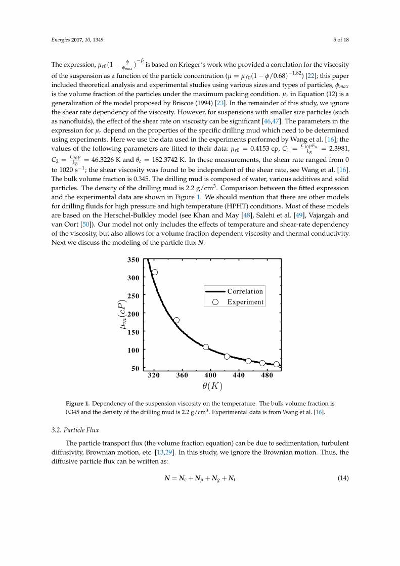
is the volume fraction of the particles under the maximum packing condition. µr in Equation (12) is ageneralization of the model proposed by Briscoe (1994) [23]. In the remainder of this study, we ignorethe shear rate dependency of the viscosity. However, for suspensions with smaller size particles (suchas nanofluids), the effect of the shear rate on viscosity can be significant [46,47]. The parameters in theexpression for µr depend on the properties of the specific drilling mud which need to be determinedusing experiments. Here we use the data used in the experiments performed by Wang et al. [16]; thevalues of the following parameters are fitted to their data: µr0 = 0.4153 cp, C1 = C10 pEu

kB= 2.3981,

C2 = C20 pkB

= 46.3226 K and θc = 182.3742 K. In these measurements, the shear rate ranged from 0to 1020 s−1; the shear viscosity was found to be independent of the shear rate, see Wang et al. [16].The bulk volume fraction is 0.345. The drilling mud is composed of water, various additives and solidparticles. The density of the drilling mud is 2.2 g/cm3. Comparison between the fitted expressionand the experimental data are shown in Figure 1. We should mention that there are other modelsfor drilling fluids for high pressure and high temperature (HPHT) conditions. Most of these modelsare based on the Herschel-Bulkley model (see Khan and May [48], Salehi et al. [49], Vajargah andvan Oort [50]). Our model not only includes the effects of temperature and shear-rate dependencyof the viscosity, but also allows for a volume fraction dependent viscosity and thermal conductivity.Next we discuss the modeling of the particle flux N.

Energies 2017, 10, 1349 5 of 17

Khan and May [48], Salehi et al. [49], Vajargah and van Oort [50]). Our model not only includes the effects of temperature and shear-rate dependency of the viscosity, but also allows for a volume fraction dependent viscosity and thermal conductivity. Next we discuss the modeling of the particle flux .

Figure 1. Dependency of the suspension viscosity on the temperature. The bulk volume fraction is 0.345 and the density of the drilling mud is 2.2 g/cm3. Experimental data is from Wang et al. [16].

3.2. Particle Flux

The particle transport flux (the volume fraction equation) can be due to sedimentation, turbulent diffusivity, Brownian motion, etc. [13,29]. In this study, we ignore the Brownian motion. Thus, the diffusive particle flux can be written as: = + + + (14)

where , , and are the contributions due to particles collision, spatial variations in the viscosity, gravity and turbulence, respectively. In this paper, we also assume = . Based on the proposal of Phillips et al. [29], we assume and are given by: = − ( ) (15) = − (ln ) (16) = (2 ) / = ( ) (17)

where is the radius of the particle, is the local shear rate, is the effective viscosity, and , are empirically-determined coefficients. According to Seifu et al. [51] the above two terms in the particle flux are given by, + = − / (18)

We can see that / is a field potential incorporating mechanism which can cause migration of the particles. Following the Phillips et al. and Subia et al. [13,29], in this paper we assumed that = 0.43, = 0.62, as constants.

The turbulent diffusivity flux is given by [52], = − ( ) (19)

where is the eddy diffusivity and is the Schmidt number assumed to be 0.9 for the present study [53,54].

Figure 1. Dependency of the suspension viscosity on the temperature. The bulk volume fraction is0.345 and the density of the drilling mud is 2.2 g/cm3. Experimental data is from Wang et al. [16].

3.2. Particle Flux

The particle transport flux (the volume fraction equation) can be due to sedimentation, turbulentdiffusivity, Brownian motion, etc. [13,29]. In this study, we ignore the Brownian motion. Thus, thediffusive particle flux can be written as:

N = Nc + Nµ + Ng + Nt (14)

Energies 2017, 10, 1349 6 of 18

where Nc, Nµ, Ng and Nt are the contributions due to particles collision, spatial variations in theviscosity, gravity and turbulence, respectively. In this paper, we also assume Ng = 0. Based on theproposal of Phillips et al. [29], we assume Nc and Nµ are given by:

Nc = −a2φKcO(.γφ) (15)

Nµ = −a2φ2 .γKµO(lnµs) (16)

.γ = (2DijDij)

1/2 = (Π)2 (17)

where a is the radius of the particle,.γ is the local shear rate, µs is the effective viscosity, and Kc, Kµ are

empirically-determined coefficients. According to Seifu et al. [51] the above two terms in the particleflux are given by,

Nc + Nµ = −a2Kcφ2 .γO(ln(

.γφµs

Kµ/Kc)) (18)

We can see that ln(.γφµs

Kµ/Kc) is a field potential incorporating mechanism which can causemigration of the particles. Following the Phillips et al. and Subia et al. [13,29], in this paper weassumed that Kc = 0.43, Kµ = 0.62, as constants.

The turbulent diffusivity flux is given by [52],

Nt = − νt

ScO(φ) (19)

where νt is the eddy diffusivity and Sc is the Schmidt number assumed to be 0.9 for thepresent study [53,54].

3.3. Heat Flux Vector

As stated by Fourier [55] (see also Winterton [56]), the heat flux vector is proportional to thegradient of temperature,

q = −kOθ (20)

where k is the thermal conductivity of the material [36]. For complex materials, k can depend on variousparameters/fields, such as concentration, temperature, shear rate, etc.; in these situations k is usuallyreplaced with km or ke f f , called the effective thermal conductivity. In general, k is a second ordertensor for anisotropic materials (for more information see [57], p. 129 and [58–60]). When turbulence isconsidered, there is an additional contribution to the conduction usually designated as kt [61,62],

k = km + kt = km +νt

Prtρ f (21)

where Prt is the Prandtl number and can be chosen as 8/9 [61]. An effective thermal conductivitymodel derived by Jeffrey [26] is:

km = κ f [1 + 3ξφ + ξφ2] + O(φ3) (22)

where:

ξ = 3ξ2 +3ξ3

4+

9ξ3

16

(ω + 2

2ω + 3

)+

3ξ4

26+ . . . (23)

where:ξ =

ω − 1ω + 2

(24)

Energies 2017, 10, 1349 7 of 18

Jeffrey’s model includes second order effects in the volume fraction, see also [63]. It is worthmentioning that Equation (22) is a (corrected) linearization of the Maxwell formula, which can berewritten as,

km = κ f1 + 2ξφ

1 − ξφ(25)

For more information about the effective heat conductivity of suspensions, see [64]. In our paperhere, we use the model proposed by Jeffrey [26]. The heat conductivity of the suspending fluid (water),κ f , is assumed to be 0.6485 W/(m·K) [65].

In the following section, we present the three-dimensional forms of the governing equations.After non-dimensionalizing these equations, we study two different problems (1) flow in a long verticalpipe; and (2) flow between two eccentric rotating cylinders. For each geometry, we first study problemswith isothermal condition, and then we look at the effect of the temperature, namely problems withnon-uniform temperature distribution.

4. Results and Discussion

Substituting Equations (13)–(14), (14)–(19) and (20)–(24) in Equations (1)–(5), a set of partialdifferential equations (PDEs) are obtained. The PDEs are given below:

div(v) = 0 (26)

ρm

(∂v∂t

+ (grad v)v)= −grad p + div ((µt + µm)D) (27)

∂φ∂t + v ∂φ

∂x = div(a2φKc.γO(φ)) + div(a2φKc(

.γ)Oφ + a2 .

γKµO(lnµm)φ2)

+div( νt

ScO(φ)) (28)

((1 − φ)ρ f 0Cp f 0 + φρs0Cps0

)(∂θ∂t + (grad θ)v

)= ((µt + µm)D) : L + div

((νtρ fPrt

+ κ f (1 + 3ξφ + ξφ2))Oθ) (29)

The above equations are used to solve for the unknowns which are, v, p, φ and θ.The dimensionless forms of the above equations are,

div(V) = 0 (30)

ρm

(∂V∂τ

+ (grad V)V)= −gradP +

1Re

div((µt + µm)

µrD)

(31)

∂φ

∂τ+ Vgradφ = div(JcΓφO(φ)) + div

(JcO(Γ)φ2 + JµΓ

O(µm)

µmφ2)+ div

(νt

ScHu0O(φ)

)(32)

(αρ f 0Cp f 0 + φρs0Cps0)(

∂θ∂τ + (grad θ)V

)= R

((µt+µm)

µrD)

: L + 1RePr div

(κt+κm

κ fOθ) (33)

where:

Y =y

Hr; X =

xHr

; Z =z

Hr; V =

vu0

; τ =tu0

Hr; θ =

θ − θ0

θ1 − θ0; Γ =

Hr.γ

u0;

ρ∗m =ρm

ρ f 0; ρ∗f 0 =

ρ f 0

ρ f 0; ρ∗s0 =

ρs0

ρ f 0; C∗

p f 0 =Cp f 0

Cp f 0; C∗

ps0 =Cps0

Cp f 0;

div∗(·) = Hrdiv(·); grad∗(·) = Hrgrad(·);

L∗ = grad∗V; D∗ =12[grad∗V + (grad∗V)T];

Energies 2017, 10, 1349 8 of 18

P∗ =p

ρ f 0u20

; Re =ρ f 0u0Hr

µr; Jc =

a2Kc

Hr2 ; Jµ =

a2Kµ

Hr2 ;

Ds =µru0

Hrρ f 0Cp f 0(θ1 − θ0); Pr =

Cp f 0µr

k f;

where Hr is a reference length, for example, the diameter of the pipe, u0 is a reference velocity andis chosen as the axial mean velocity at the inlet, and θ1 and θ0 are reference temperatures and arechosen as 393 K and 293 K, respectively. The asterisks have been dropped for simplicity. Among theabove dimensionless numbers Jc and Jµ are related to the particles flux; Ds is related to the heatdissipation. For obtaining the turbulent eddy diffusivity νt (and the turbulent eddy viscosity µt),different turbulence models, such as k − ω or k − ε RANS model, can be selected depending on theflow conditions [66–68]. In this paper, we also ignore the effect of the turbulence, due to the lowReynolds number of the problems studied. Table 1 lists the value of the physical properties appliedin this paper. The suspension viscosity, effective thermal conductivity and Kc are calculated by themodels/correlations discussed in the previous section.

Numerically, the above governing equations are solved by developing PDE solver using thelibraries of OpenFOAM® [69]. The PIMPLE algorithm is applied for dealing with the incompressibilitycondition [69]. The details of how the governing equations are discretized in OpenFOAM, the PIMPLEalgorithm, the numerical schemes, etc., are given on [69–73]. For ensuring numerical stability andaccuracy, the value of the time step is chosen so that the maximum Courant Number is always lessthan 0.1. The Courant Number is the portion of a cell that a material will transport by advection in onetime step. The boundary conditions are provided in Table 2, for more detail see [71]. For each problem,the simulation domain is discretized as hexahedral meshes using ICEM [74]. The mesh-dependencestudies are performed for each case.

In the following cases studied, we assume Ds = 0, that is we ignore the effect of viscous dissipation;and due to the low Reynolds number of the problems we also ignore the effect of the turbulence onflow, heat transfer and particles transport.

Table 1. Physical properties used in this paper [29,65,75,76].

Physical Property Value Physical Property Value

ρ f 0 1000 kg/m3 cp f 0 4020 J/(kg·K)ρs0 4480 kg/m3 cps0 460 J/(kg·K)a 1.25 mm κ f 0.6485 W/(m·K)

Kµ 0.62 ω 2.0

Table 2. Boundary conditions. For more discussion on the boundary condition, see [71].

Boundary Pressure Velocity Volume Fraction Temperature

Wall Fixed flux (0) Fixed value Fixed flux (0) Fixed valueInlet Fixed value (0) Fixed value Fixed value (0) Fixed value

Outlet Fixed value (0) Fixed flux (0) Fixed flux (0) Fixed flux (0)

4.1. Vertical Flow in a Pipe

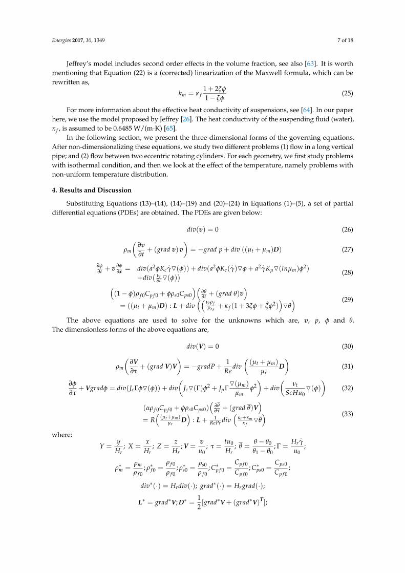
First, we study the flow in a vertical pipe, as shown in Figure 2. The pipe is assumed to beembedded in earth. To save computational cost while simulating the flow in a long pipe, we usethe symmetry condition and assume that the flow is two dimensional. Furthermore, to ensurea steady-state condition, the simulation time is always set to be greater than 5·(L/U), where L is thelength of the pipe and U is the mean velocity of the flow.

Energies 2017, 10, 1349 9 of 18

Energies 2017, 10, 1349 8 of 17

detail see [71]. For each problem, the simulation domain is discretized as hexahedral meshes using ICEM [74]. The mesh-dependence studies are performed for each case.

In the following cases studied, we assume = 0 , that is we ignore the effect of viscous dissipation; and due to the low Reynolds number of the problems we also ignore the effect of the turbulence on flow, heat transfer and particles transport.

Table 1. Physical properties used in this paper [29,65,75,76].

Physical Property Value Physical Property Value 1000 kg/m3 4020 J/(kg·K) 4480 kg/m3 460 J/(kg·K)

1.25 mm 0.6485 W/(m·K) 0.62 2.0

Table 2. Boundary conditions. For more discussion on the boundary condition, see [71].

Boundary Pressure Velocity Volume Fraction Temperature Wall Fixed flux (0) Fixed value Fixed flux (0) Fixed value Inlet Fixed value (0) Fixed value Fixed value (0) Fixed value

Outlet Fixed value (0) Fixed flux (0) Fixed flux (0) Fixed flux (0)

4.1. Vertical Flow in a Pipe

First, we study the flow in a vertical pipe, as shown in Figure 2. The pipe is assumed to be embedded in earth. To save computational cost while simulating the flow in a long pipe, we use the symmetry condition and assume that the flow is two dimensional. Furthermore, to ensure a steady-state condition, the simulation time is always set to be greater than 5·(L/U), where L is the length of the pipe and U is the mean velocity of the flow.

Figure 2. Schematic of the pipe.

4.1.1. Effect of Bulk Volume Fraction and the Reynolds Number

From Equation (11) we can see that the concentration of the solid particles affects the viscosity of the suspension, especially when the volume fraction is close to the maximum packing volume fraction. We assume isothermal conditions, i.e., is zero. Based on the flow conditions at the inlet, the values of the dimensionless numbers are: = 159, = 3.87 × 10 and = 971. Here the

Figure 2. Schematic of the pipe.

4.1.1. Effect of Bulk Volume Fraction and the Reynolds Number

From Equation (11) we can see that the concentration of the solid particles affects the viscosity ofthe suspension, especially when the volume fraction is close to the maximum packing volume fraction.We assume isothermal conditions, i.e., θ is zero. Based on the flow conditions at the inlet, the valuesof the dimensionless numbers are: Re = 159, Jµ = 3.87 × 10−4 and Pr = 971. Here the characteristiclength Hr is chosen as the diameter of the pipe, D. The length of the pipe is L = 100D, for ensuringthat the flow is fully developed.

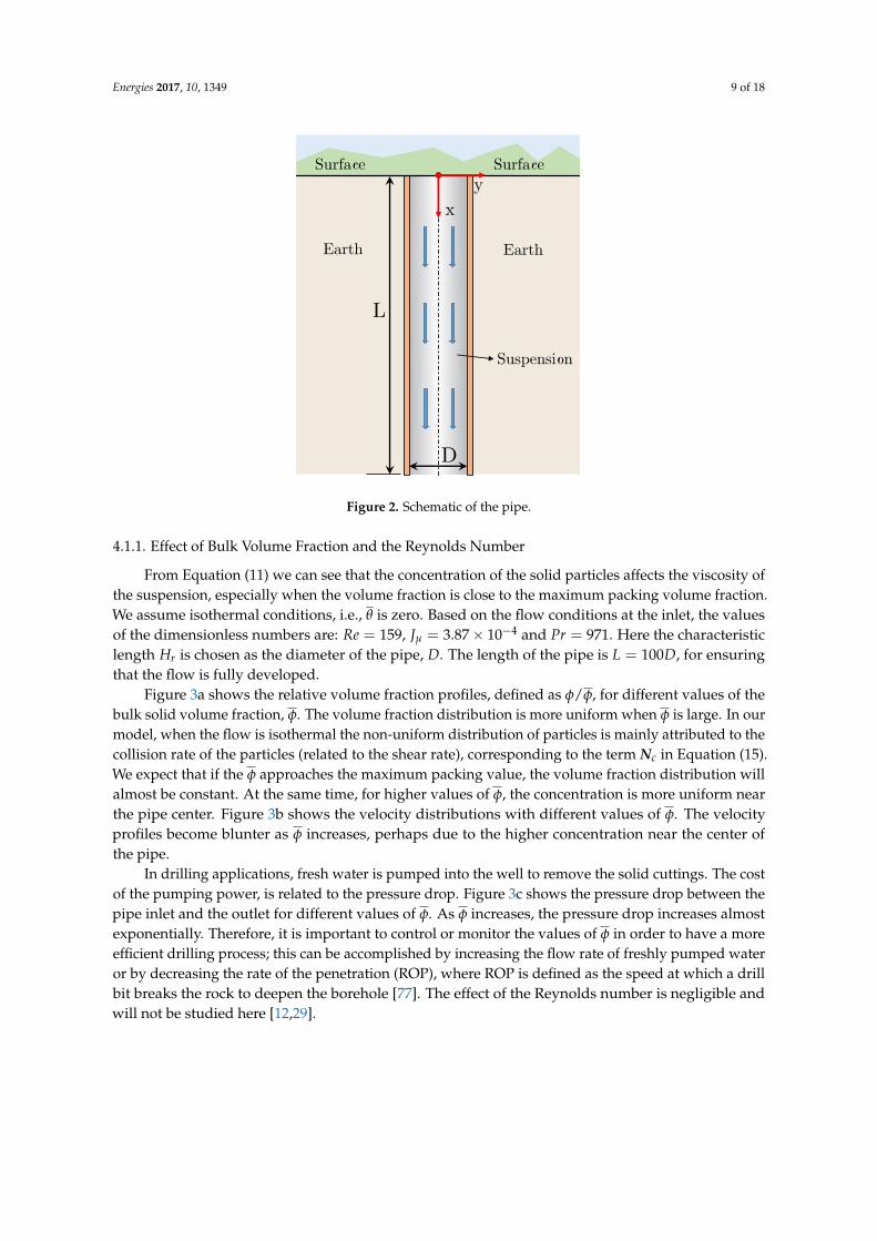
Figure 3a shows the relative volume fraction profiles, defined as φ/φ, for different values of thebulk solid volume fraction, φ. The volume fraction distribution is more uniform when φ is large. In ourmodel, when the flow is isothermal the non-uniform distribution of particles is mainly attributed to thecollision rate of the particles (related to the shear rate), corresponding to the term Nc in Equation (15).We expect that if the φ approaches the maximum packing value, the volume fraction distribution willalmost be constant. At the same time, for higher values of φ, the concentration is more uniform nearthe pipe center. Figure 3b shows the velocity distributions with different values of φ. The velocityprofiles become blunter as φ increases, perhaps due to the higher concentration near the center ofthe pipe.

In drilling applications, fresh water is pumped into the well to remove the solid cuttings. The costof the pumping power, is related to the pressure drop. Figure 3c shows the pressure drop between thepipe inlet and the outlet for different values of φ. As φ increases, the pressure drop increases almostexponentially. Therefore, it is important to control or monitor the values of φ in order to have a moreefficient drilling process; this can be accomplished by increasing the flow rate of freshly pumped wateror by decreasing the rate of the penetration (ROP), where ROP is defined as the speed at which a drillbit breaks the rock to deepen the borehole [77]. The effect of the Reynolds number is negligible andwill not be studied here [12,29].

Energies 2017, 10, 1349 10 of 18

Energies 2017, 10, 1349 9 of 17

characteristic length is chosen as the diameter of the pipe, . The length of the pipe is = 100 , for ensuring that the flow is fully developed.

Figure 3a shows the relative volume fraction profiles, defined as / , for different values of the bulk solid volume fraction, . The volume fraction distribution is more uniform when is large. In our model, when the flow is isothermal the non-uniform distribution of particles is mainly attributed to the collision rate of the particles (related to the shear rate), corresponding to the term in Equation (15). We expect that if the approaches the maximum packing value, the volume fraction distribution will almost be constant. At the same time, for higher values of , the concentration is more uniform near the pipe center. Figure 3b shows the velocity distributions with different values of . The velocity profiles become blunter as increases, perhaps due to the higher concentration near the center of the pipe.

In drilling applications, fresh water is pumped into the well to remove the solid cuttings. The cost of the pumping power, is related to the pressure drop. Figure 3c shows the pressure drop between the pipe inlet and the outlet for different values of . As increases, the pressure drop increases almost exponentially. Therefore, it is important to control or monitor the values of in order to have a more efficient drilling process; this can be accomplished by increasing the flow rate of freshly pumped water or by decreasing the rate of the penetration (ROP), where ROP is defined as the speed at which a drill bit breaks the rock to deepen the borehole [77]. The effect of the Reynolds number is negligible and will not be studied here [12,29].

Figure 3. (a) The relative volume fraction profiles along the radial direction (Y direction as shown in Figure 2.) for different values of the bulk volume fraction, ; (b) The profiles of the axial (X-direction) velocity, , along the radial direction; (c) pressure drop between the inlet and the outlet for different values of the bulk volume fraction . = 159, = 3.87 × 10 and = 971.

4.1.2. Effect of Temperature in the Axial Direction

Figure 3. (a) The relative volume fraction profiles along the radial direction (Y direction as shown inFigure 2.) for different values of the bulk volume fraction, φ; (b) The profiles of the axial (X-direction)velocity, Vx, along the radial direction; (c) pressure drop between the inlet and the outlet for differentvalues of the bulk volume fraction φ. Re = 159, Jµ = 3.87 × 10−4 and Pr = 971.

4.1.2. Effect of Temperature in the Axial Direction

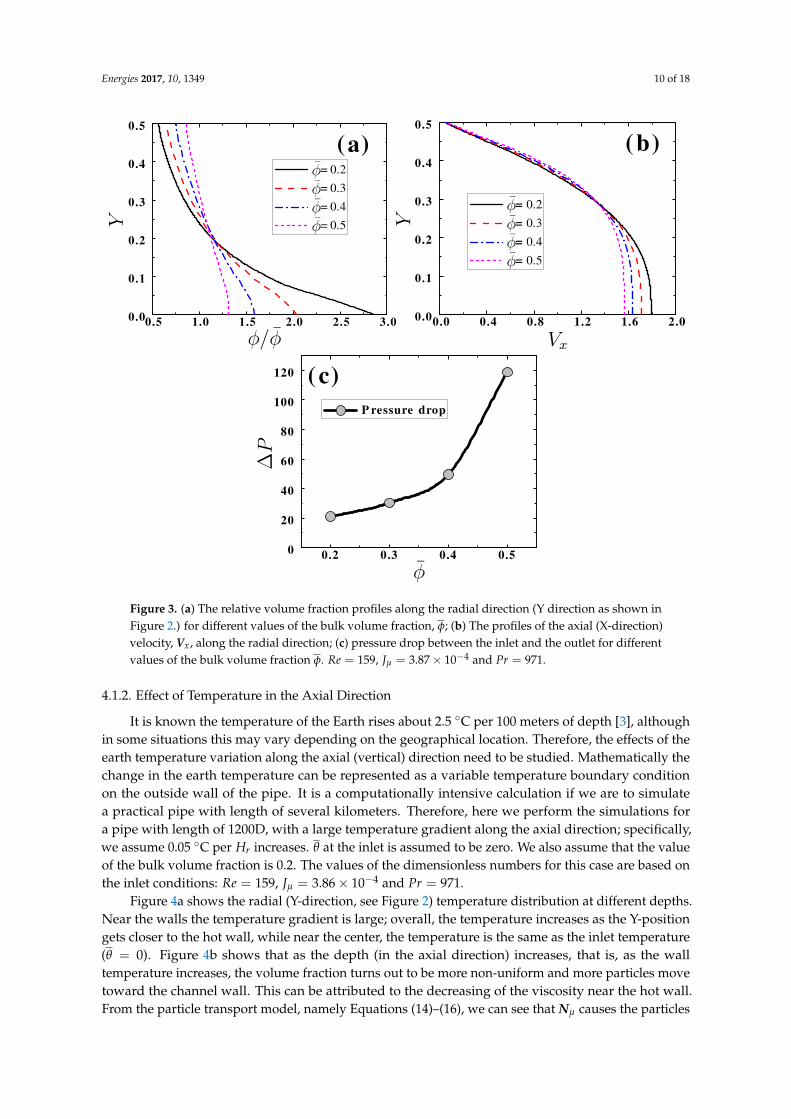
It is known the temperature of the Earth rises about 2.5 C per 100 meters of depth [3], althoughin some situations this may vary depending on the geographical location. Therefore, the effects of theearth temperature variation along the axial (vertical) direction need to be studied. Mathematically thechange in the earth temperature can be represented as a variable temperature boundary conditionon the outside wall of the pipe. It is a computationally intensive calculation if we are to simulatea practical pipe with length of several kilometers. Therefore, here we perform the simulations fora pipe with length of 1200D, with a large temperature gradient along the axial direction; specifically,we assume 0.05 C per Hr increases. θ at the inlet is assumed to be zero. We also assume that the valueof the bulk volume fraction is 0.2. The values of the dimensionless numbers for this case are based onthe inlet conditions: Re = 159, Jµ = 3.86 × 10−4 and Pr = 971.

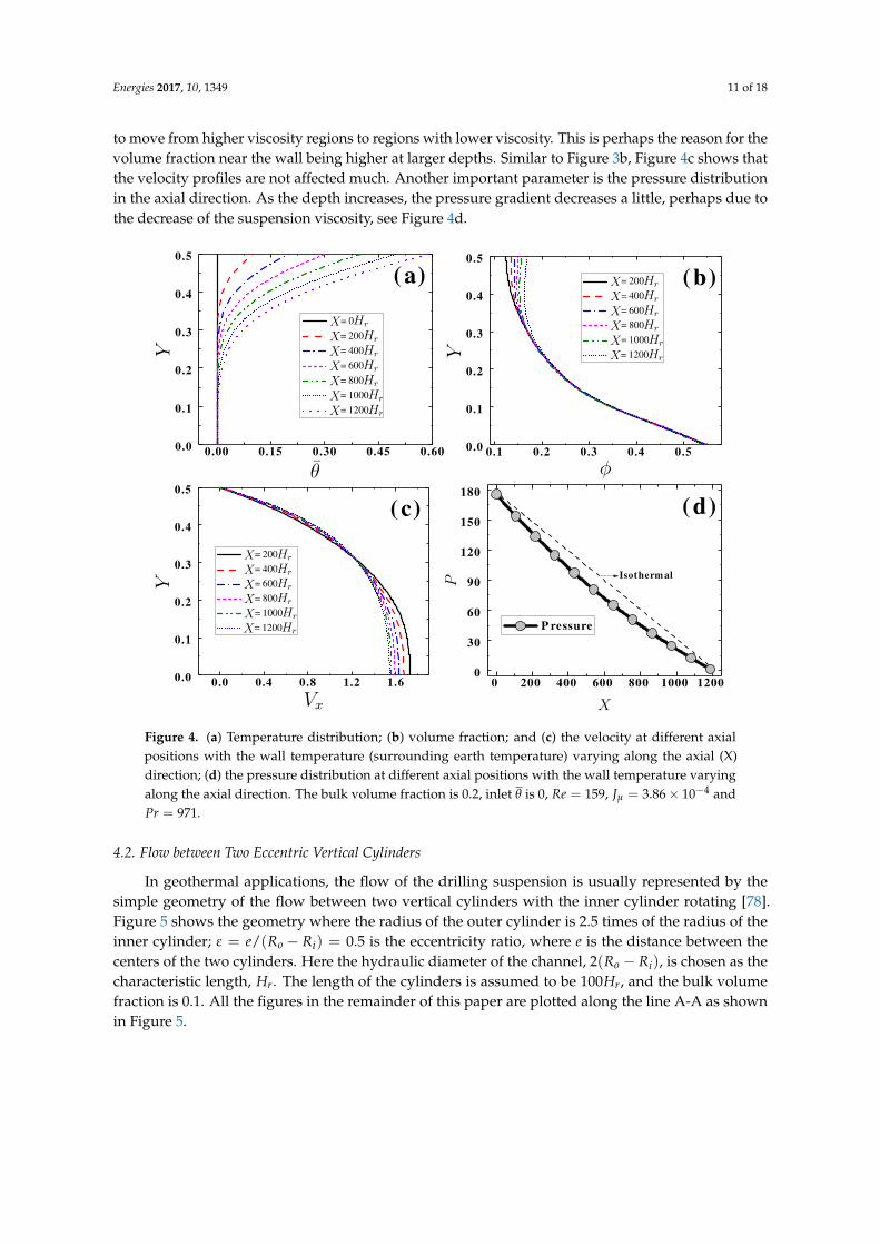
Figure 4a shows the radial (Y-direction, see Figure 2) temperature distribution at different depths.Near the walls the temperature gradient is large; overall, the temperature increases as the Y-positiongets closer to the hot wall, while near the center, the temperature is the same as the inlet temperature(θ = 0). Figure 4b shows that as the depth (in the axial direction) increases, that is, as the walltemperature increases, the volume fraction turns out to be more non-uniform and more particles movetoward the channel wall. This can be attributed to the decreasing of the viscosity near the hot wall.From the particle transport model, namely Equations (14)–(16), we can see that Nµ causes the particles

Energies 2017, 10, 1349 11 of 18

to move from higher viscosity regions to regions with lower viscosity. This is perhaps the reason for thevolume fraction near the wall being higher at larger depths. Similar to Figure 3b, Figure 4c shows thatthe velocity profiles are not affected much. Another important parameter is the pressure distributionin the axial direction. As the depth increases, the pressure gradient decreases a little, perhaps due tothe decrease of the suspension viscosity, see Figure 4d.

Energies 2017, 10, 1349 10 of 17

It is known the temperature of the Earth rises about 2.5 per 100 meters of depth [3], although in some situations this may vary depending on the geographical location. Therefore, the effects of the earth temperature variation along the axial (vertical) direction need to be studied. Mathematically the change in the earth temperature can be represented as a variable temperature boundary condition on the outside wall of the pipe. It is a computationally intensive calculation if we are to simulate a practical pipe with length of several kilometers. Therefore, here we perform the simulations for a pipe with length of 1200D, with a large temperature gradient along the axial direction; specifically, we assume 0.05 per increases. at the inlet is assumed to be zero. We also assume that the value of the bulk volume fraction is 0.2. The values of the dimensionless numbers for this case are based on the inlet conditions: = 159, = 3.86 × 10 and = 971.

Figure 4a shows the radial (Y-direction, see Figure 2) temperature distribution at different depths. Near the walls the temperature gradient is large; overall, the temperature increases as the Y-position gets closer to the hot wall, while near the center, the temperature is the same as the inlet temperature ( = 0). Figure 4b shows that as the depth (in the axial direction) increases, that is, as the wall temperature increases, the volume fraction turns out to be more non-uniform and more particles move toward the channel wall. This can be attributed to the decreasing of the viscosity near the hot wall. From the particle transport model, namely Equations (14)–(16), we can see that causes the particles to move from higher viscosity regions to regions with lower viscosity. This is perhaps the reason for the volume fraction near the wall being higher at larger depths. Similar to Figure 3b, Figure 4c shows that the velocity profiles are not affected much. Another important parameter is the pressure distribution in the axial direction. As the depth increases, the pressure gradient decreases a little, perhaps due to the decrease of the suspension viscosity, see Figure 4d.

Figure 4. (a) Temperature distribution; (b) volume fraction; and (c) the velocity at different axial positions with the wall temperature (surrounding earth temperature) varying along the axial (X) direction; (d) the pressure distribution at different axial positions with the wall temperature varying along the axial direction. The bulk volume fraction is 0.2, inlet is 0, = 159, = 3.86 × 10 and = 971.

Figure 4. (a) Temperature distribution; (b) volume fraction; and (c) the velocity at different axialpositions with the wall temperature (surrounding earth temperature) varying along the axial (X)direction; (d) the pressure distribution at different axial positions with the wall temperature varyingalong the axial direction. The bulk volume fraction is 0.2, inlet θ is 0, Re = 159, Jµ = 3.86 × 10−4 andPr = 971.

4.2. Flow between Two Eccentric Vertical Cylinders

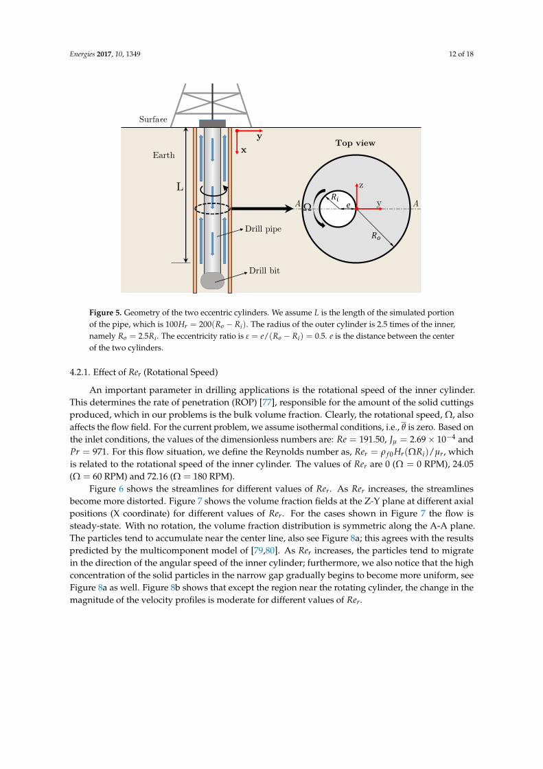
In geothermal applications, the flow of the drilling suspension is usually represented by thesimple geometry of the flow between two vertical cylinders with the inner cylinder rotating [78].Figure 5 shows the geometry where the radius of the outer cylinder is 2.5 times of the radius of theinner cylinder; ε = e/(Ro − Ri) = 0.5 is the eccentricity ratio, where e is the distance between thecenters of the two cylinders. Here the hydraulic diameter of the channel, 2(Ro − Ri), is chosen as thecharacteristic length, Hr. The length of the cylinders is assumed to be 100Hr, and the bulk volumefraction is 0.1. All the figures in the remainder of this paper are plotted along the line A-A as shownin Figure 5.

Energies 2017, 10, 1349 12 of 18

Energies 2017, 10, 1349 11 of 17

4.2. Flow between Two Eccentric Vertical Cylinders

In geothermal applications, the flow of the drilling suspension is usually represented by the simple geometry of the flow between two vertical cylinders with the inner cylinder rotating [78]. Figure 5 shows the geometry where the radius of the outer cylinder is 2.5 times of the radius of the inner cylinder; = /( − ) = 0.5 is the eccentricity ratio, where is the distance between the centers of the two cylinders. Here the hydraulic diameter of the channel, 2( − ), is chosen as the characteristic length, . The length of the cylinders is assumed to be 100 , and the bulk volume fraction is 0.1. All the figures in the remainder of this paper are plotted along the line A-A as shown in Figure 5.

Figure 5. Geometry of the two eccentric cylinders. We assume is the length of the simulated portion of the pipe, which is 100 = 200( − ). The radius of the outer cylinder is 2.5 times of the inner, namely = 2.5 . The eccentricity ratio is = /( − ) = 0.5. is the distance between the center of the two cylinders.

4.2.1. Effect of (Rotational Speed)

An important parameter in drilling applications is the rotational speed of the inner cylinder. This determines the rate of penetration (ROP) [77], responsible for the amount of the solid cuttings produced, which in our problems is the bulk volume fraction. Clearly, the rotational speed, Ω, also affects the flow field. For the current problem, we assume isothermal conditions, i.e., is zero. Based on the inlet conditions, the values of the dimensionless numbers are: = 191.50, = 2.69 × 10 and = 971. For this flow situation, we define the Reynolds number as, = (Ω )/ , which is related to the rotational speed of the inner cylinder. The values of are 0 (Ω = 0 RPM), 24.05 (Ω = 60 RPM) and 72.16 (Ω = 180 RPM).

Figure 6 shows the streamlines for different values of . As increases, the streamlines become more distorted. Figure 7 shows the volume fraction fields at the Z-Y plane at different axial positions (X coordinate) for different values of . For the cases shown in Figure 7 the flow is steady-state. With no rotation, the volume fraction distribution is symmetric along the A-A plane. The particles tend to accumulate near the center line, also see Figure 8a; this agrees with the results predicted by the multicomponent model of [79,80]. As increases, the particles tend to migrate in the direction of the angular speed of the inner cylinder; furthermore, we also notice that the high concentration of the solid particles in the narrow gap gradually begins to become more uniform, see Figure 8a as well. Figure 8b shows that except the region near the rotating cylinder, the change in the magnitude of the velocity profiles is moderate for different values of .

Figure 5. Geometry of the two eccentric cylinders. We assume L is the length of the simulated portionof the pipe, which is 100Hr = 200(Ro − Ri). The radius of the outer cylinder is 2.5 times of the inner,namely Ro = 2.5Ri. The eccentricity ratio is ε = e/(Ro − Ri) = 0.5. e is the distance between the centerof the two cylinders.

4.2.1. Effect of Rer (Rotational Speed)

An important parameter in drilling applications is the rotational speed of the inner cylinder.This determines the rate of penetration (ROP) [77], responsible for the amount of the solid cuttingsproduced, which in our problems is the bulk volume fraction. Clearly, the rotational speed, Ω, alsoaffects the flow field. For the current problem, we assume isothermal conditions, i.e., θ is zero. Based onthe inlet conditions, the values of the dimensionless numbers are: Re = 191.50, Jµ = 2.69 × 10−4 andPr = 971. For this flow situation, we define the Reynolds number as, Rer = ρ f 0Hr(ΩRi)/µr, whichis related to the rotational speed of the inner cylinder. The values of Rer are 0 (Ω = 0 RPM), 24.05(Ω = 60 RPM) and 72.16 (Ω = 180 RPM).

Figure 6 shows the streamlines for different values of Rer. As Rer increases, the streamlinesbecome more distorted. Figure 7 shows the volume fraction fields at the Z-Y plane at different axialpositions (X coordinate) for different values of Rer. For the cases shown in Figure 7 the flow issteady-state. With no rotation, the volume fraction distribution is symmetric along the A-A plane.The particles tend to accumulate near the center line, also see Figure 8a; this agrees with the resultspredicted by the multicomponent model of [79,80]. As Rer increases, the particles tend to migratein the direction of the angular speed of the inner cylinder; furthermore, we also notice that the highconcentration of the solid particles in the narrow gap gradually begins to become more uniform, seeFigure 8a as well. Figure 8b shows that except the region near the rotating cylinder, the change in themagnitude of the velocity profiles is moderate for different values of Rer.

Energies 2017, 10, 1349 13 of 18

Energies 2017, 10, 1349 12 of 17

Figure 6. Streamlines for the isothermal flow between the two eccentric cylinders with different values of (related to the rotational speed).

Figure 7. Top view. The volume fraction fields in the Z-Y plane for different dimensionless axial positions (X-direction) for different (rotational speed). The rotation is counter clockwise.

Figure 8. (a) The volume fraction and (b) the velocity profiles along the A-A plane (see Figure 5 also) near the outlet for different .

4.2.2. Effects of the Earth Temperature

Cylinder walls Cylinder walls

Figure 6. Streamlines for the isothermal flow between the two eccentric cylinders with different valuesof Rer (related to the rotational speed).

Energies 2017, 10, 1349 12 of 17

Figure 6. Streamlines for the isothermal flow between the two eccentric cylinders with different values of (related to the rotational speed).

Figure 7. Top view. The volume fraction fields in the Z-Y plane for different dimensionless axial positions (X-direction) for different (rotational speed). The rotation is counter clockwise.

Figure 8. (a) The volume fraction and (b) the velocity profiles along the A-A plane (see Figure 5 also) near the outlet for different .

4.2.2. Effects of the Earth Temperature

Cylinder walls Cylinder walls

Figure 7. Top view. The volume fraction fields in the Z-Y plane for different dimensionless axialpositions (X-direction) for different Rer (rotational speed). The rotation is counter clockwise.

Energies 2017, 10, 1349 12 of 17

Figure 6. Streamlines for the isothermal flow between the two eccentric cylinders with different values of (related to the rotational speed).

Figure 7. Top view. The volume fraction fields in the Z-Y plane for different dimensionless axial positions (X-direction) for different (rotational speed). The rotation is counter clockwise.

Figure 8. (a) The volume fraction and (b) the velocity profiles along the A-A plane (see Figure 5 also) near the outlet for different .

4.2.2. Effects of the Earth Temperature

Cylinder walls Cylinder walls

Figure 8. (a) The volume fraction and (b) the velocity profiles along the A-A plane (see Figure 5 also)near the outlet for different Rer.

Energies 2017, 10, 1349 14 of 18

4.2.2. Effects of the Earth Temperature

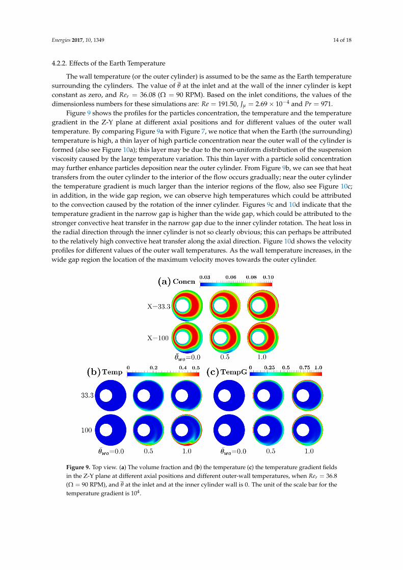
The wall temperature (or the outer cylinder) is assumed to be the same as the Earth temperaturesurrounding the cylinders. The value of θ at the inlet and at the wall of the inner cylinder is keptconstant as zero, and Rer = 36.08 (Ω = 90 RPM). Based on the inlet conditions, the values of thedimensionless numbers for these simulations are: Re = 191.50, Jµ = 2.69 × 10−4 and Pr = 971.

Figure 9 shows the profiles for the particles concentration, the temperature and the temperaturegradient in the Z-Y plane at different axial positions and for different values of the outer walltemperature. By comparing Figure 9a with Figure 7, we notice that when the Earth (the surrounding)temperature is high, a thin layer of high particle concentration near the outer wall of the cylinder isformed (also see Figure 10a); this layer may be due to the non-uniform distribution of the suspensionviscosity caused by the large temperature variation. This thin layer with a particle solid concentrationmay further enhance particles deposition near the outer cylinder. From Figure 9b, we can see that heattransfers from the outer cylinder to the interior of the flow occurs gradually; near the outer cylinderthe temperature gradient is much larger than the interior regions of the flow, also see Figure 10c;in addition, in the wide gap region, we can observe high temperatures which could be attributedto the convection caused by the rotation of the inner cylinder. Figures 9c and 10d indicate that thetemperature gradient in the narrow gap is higher than the wide gap, which could be attributed to thestronger convective heat transfer in the narrow gap due to the inner cylinder rotation. The heat loss inthe radial direction through the inner cylinder is not so clearly obvious; this can perhaps be attributedto the relatively high convective heat transfer along the axial direction. Figure 10d shows the velocityprofiles for different values of the outer wall temperatures. As the wall temperature increases, in thewide gap region the location of the maximum velocity moves towards the outer cylinder.

Energies 2017, 10, 1349 13 of 17

The wall temperature (or the outer cylinder) is assumed to be the same as the Earth temperature surrounding the cylinders. The value of at the inlet and at the wall of the inner cylinder is kept constant as zero, and = 36.08 (Ω = 90 RPM). Based on the inlet conditions, the values of the dimensionless numbers for these simulations are: = 191.50, = 2.69 × 10 and = 971.

Figure 9 shows the profiles for the particles concentration, the temperature and the temperature gradient in the Z-Y plane at different axial positions and for different values of the outer wall temperature. By comparing Figure 9a with Figure 7, we notice that when the Earth (the surrounding) temperature is high, a thin layer of high particle concentration near the outer wall of the cylinder is formed (also see Figure 10a); this layer may be due to the non-uniform distribution of the suspension viscosity caused by the large temperature variation. This thin layer with a particle solid concentration may further enhance particles deposition near the outer cylinder. From Figure 9b, we can see that heat transfers from the outer cylinder to the interior of the flow occurs gradually; near the outer cylinder the temperature gradient is much larger than the interior regions of the flow, also see Figure 10c; in addition, in the wide gap region, we can observe high temperatures which could be attributed to the convection caused by the rotation of the inner cylinder. Figure 9c and Figure 10d indicate that the temperature gradient in the narrow gap is higher than the wide gap, which could be attributed to the stronger convective heat transfer in the narrow gap due to the inner cylinder rotation. The heat loss in the radial direction through the inner cylinder is not so clearly obvious; this can perhaps be attributed to the relatively high convective heat transfer along the axial direction. Figure 10d shows the velocity profiles for different values of the outer wall temperatures. As the wall temperature increases, in the wide gap region the location of the maximum velocity moves towards the outer cylinder.

Figure 9. Top view. (a) The volume fraction and (b) the temperature (c) the temperature gradient fields in the Z-Y plane at different axial positions and different outer-wall temperatures, when =36.8 (Ω = 90 RPM), and at the inlet and at the inner cylinder wall is 0. The unit of the scale bar for the temperature gradient is 10 .

Figure 9. Top view. (a) The volume fraction and (b) the temperature (c) the temperature gradient fieldsin the Z-Y plane at different axial positions and different outer-wall temperatures, when Rer = 36.8(Ω = 90 RPM), and θ at the inlet and at the inner cylinder wall is 0. The unit of the scale bar for thetemperature gradient is 104.

Energies 2017, 10, 1349 15 of 18

Energies 2017, 10, 1349 14 of 17

Figure 10. (a) The volume fraction profiles; (b) the velocity profiles; (c) the temperature profiles and (d) the temperature gradient profiles for different values of the earth temperature (wall temperature of the outer cylinder), when = 36.8 (Ω = 90 RPM) and at the inlet and the inner cylinder wall is 0.

5. Concluding Remarks

In this study, we look at the heat transfer in a drilling fluid. The fluid is assumed to be a suspension composed of various components with complex rheological behavior. We model this suspension as a non-linear fluid, where the viscosity and the heat diffusivity depend on the concentration of the particle, the shear rate and temperature. The motion of the particles is based on a particle flux equation, where a generalization of the model proposed by [29] is used. By performing numerical studies for two different flow conditions, namely the flow in a vertical pipe and flow between two rotating cylinders with various boundary and flow conditions, we observe that the temperature and the flow fields depend significantly on the earth (surrounding) temperature distribution, the bulk volume fraction, etc. We also notice that for a large value of the (dimensionless) earth temperature, such as = 1.0, a thin layer with high particle concentration is formed near the outer cylinder, which may enhance particle deposition in that region. Furthermore, as the bulk volume fraction increases, the pressure drop increases exponentially, perhaps due to the increase in the suspension viscosity. Finally, in certain applications, especially those involving gas-particle flows, such as fluidized bed reactors, under certain conditions, there could be a counter flow situations due to high solid loading (see Bednarz, et al. [81], Das et al. [82], Garić-Grulović et al. [83]). We did not consider this phenomenon in this paper.

Author Contributions: Wei-Tao Wu developed the framework of the paper and did the numerical simulations. Mehrdad Massoudi and Wei-Tao Wu derived the equations. Wei-Tao Wu, Nadine Aubry, James F. Antaki, Mark L. McKoy, and Mehrdad Massoudi prepared the manuscript.

Cylinder walls Cylinder walls

Cylinder walls Cylinder walls

Figure 10. (a) The volume fraction profiles; (b) the velocity profiles; (c) the temperature profiles and(d) the temperature gradient profiles for different values of the earth temperature (wall temperature ofthe outer cylinder), when Rer = 36.8 (Ω = 90 RPM) and θ at the inlet and the inner cylinder wall is 0.

5. Concluding Remarks

In this study, we look at the heat transfer in a drilling fluid. The fluid is assumed to be a suspensioncomposed of various components with complex rheological behavior. We model this suspension asa non-linear fluid, where the viscosity and the heat diffusivity depend on the concentration of theparticle, the shear rate and temperature. The motion of the particles is based on a particle flux equation,where a generalization of the model proposed by [29] is used. By performing numerical studies for twodifferent flow conditions, namely the flow in a vertical pipe and flow between two rotating cylinderswith various boundary and flow conditions, we observe that the temperature and the flow fieldsdepend significantly on the earth (surrounding) temperature distribution, the bulk volume fraction,etc. We also notice that for a large value of the (dimensionless) earth temperature, such as θwo = 1.0,a thin layer with high particle concentration is formed near the outer cylinder, which may enhanceparticle deposition in that region. Furthermore, as the bulk volume fraction increases, the pressuredrop increases exponentially, perhaps due to the increase in the suspension viscosity. Finally, in certainapplications, especially those involving gas-particle flows, such as fluidized bed reactors, under certainconditions, there could be a counter flow situations due to high solid loading (see Bednarz, et al. [81],Das et al. [82], Garic-Grulovic et al. [83]). We did not consider this phenomenon in this paper.

Author Contributions: Wei-Tao Wu developed the framework of the paper and did the numerical simulations.Mehrdad Massoudi and Wei-Tao Wu derived the equations. Wei-Tao Wu, Nadine Aubry, James F. Antaki, Mark L.McKoy, and Mehrdad Massoudi prepared the manuscript.

Conflicts of Interest: The authors declare no conflict of interest.

References

1. Younger, P.L. Geothermal energy: Delivering on the global potential. Energies 2015, 8, 11737–11754.[CrossRef]

Energies 2017, 10, 1349 16 of 18

2. Coussot, P. Rheophysics; Springer International Publishing: Cham, Switzerland, 2014.3. Finger, J.; Blankenship, D. Handbook of Best Practices for Geothermal Drilling; Sandia National Laboratories:

Albuquerque, NM, USA, 2010.4. Sáez Blázquez, C.; Farfán Martín, A.; Martín Nieto, I.; Carrasco García, P.; Sánchez Pérez, L.; González-Aguilera, D.

Efficiency Analysis of the Main Components of a Vertical Closed-Loop System in a Borehole Heat Exchanger.Energies 2017, 10, 201.

5. Congedo, P.M.; Lorusso, C.; De Giorgi, M.G.; Marti, R.; D’Agostino, D. Horizontal Air-Ground HeatExchanger Performance and Humidity Simulation by Computational Fluid Dynamic Analysis. Energies 2016,9, 930. [CrossRef]

6. Alhamid, M.I.; Daud, Y.; Surachman, A.; Sugiyono, A.; Aditya, H.B.; Mahlia, T.M.I. Potential of geothermalenergy for electricity generation in Indonesia: A review. Renew. Sustain. Energy Rev. 2016, 53, 733–740.

7. Yavuzturk, C.; Spitler, J.D.; Rees, S.J. A transient two-dimensional finite volume model for the simulation ofvertical U-tube ground heat exchangers. ASHRAE Trans. 1999, 105, 465–474.

8. He, M.; Rees, S.; Shao, L. Simulation of a domestic ground source heat pump system usinga three-dimensional numerical borehole heat exchanger model. J. Build. Perform. Simul. 2011, 4, 141–155.[CrossRef]

9. Lund, J.W. Direct utilization of geothermal energy. Energies 2010, 3, 1443–1471. [CrossRef]10. Rabia, H. Oilwell Drilling Engineering: Principles and Practice; Graham and Trotman Ltd.: London, UK, 1985.11. Zhou, Z.; Wu, W.T.; Massoudi, M. Fully developed flow of a drilling fluid between two rotating cylinders.

Appl. Math. Comput. 2016, 281, 266–277. [CrossRef]12. Wu, W.T.; Massoudi, M. Heat Transfer and Dissipation Effects in the Flow of a Drilling Fluid. Fluids 2016, 1, 4.

[CrossRef]13. Subia, S R.; Ingber, M.S.; Mondy, L.A.; Altobelli, S.A.; Graham, A.L. Modelling of concentrated suspensions

using a continuum constitutive equation. J. Fluid Mech. 1998, 373, 193–219. [CrossRef]14. Mahto, V.; Sharma, V.P. Rheological study of a water based oil well drilling fluid. J. Pet. Sci. Eng. 2004, 45,

123–128. [CrossRef]15. Saasen, A.; Løklingholm, G. The effect of drilling fluid rheological properties on hole cleaning. In IADC/SPE

Drilling Conference; Society of Petroleum Engineers: Dallas, TX, USA, 2002.16. Wang, F.; Tan, X.; Wang, R.; Sun, M.; Wang, L.; Liu, J. High temperature and high pressure rheological

properties of high-density water-based drilling fluids for deep wells. Pet. Sci. 2012, 9, 354–362. [CrossRef]17. Rybach, L. Geothermal power growth 1995–2013—A comparison with other renewables. Energies 2014, 7,

4802–4812. [CrossRef]18. Vajravelu, K.; Sreenadh, S.; Babu, V.R. Peristaltic transport of a Herschel–Bulkley fluid in an inclined tube.

Int. J. Non Linear Mech. 2005, 40, 83–90. [CrossRef]19. Herschel, W.H.; Bulkley, R. Konsistenzmessungen von gummi-benzollösungen. Colloid Polym. Sci. 1926, 39,

291–300. [CrossRef]20. Papanastasiou, T.C. Flows of materials with yield. J. Rheol. 1987, 31, 385–404. [CrossRef]21. Alexandrou, A.N.; McGilvreay, T.M.; Burgos, G. Steady Herschel–Bulkley fluid flow in three-dimensional

expansions. J. Nonnewton. Fluid Mech. 2001, 100, 77–96. [CrossRef]22. Krieger, I.M. Rheology of monodisperse latices. Adv. Colloid Interface Sci. 1972, 3, 111–136. [CrossRef]23. Briscoe, B.J.; Luckham, P.F.; Ren, S.R. The properties of drilling muds at high pressures and high temperatures.

Philos. Trans. R. Soc. Lond. A Math. Phys. Eng. Sci. 1994, 348, 179–207. [CrossRef]24. Maxwell, J.C. A Treatise on Electricity and Magnetism, 2nd ed.; Clarendon Press: Oxford, UK, 1873.25. Hamilton, R.L.; Crosser, O.K. Thermal conductivity of heterogeneous two-component systems. Ind. Eng.

Chem. Fundam. 1962, 1, 187–191. [CrossRef]26. Jeffrey, D.J. Conduction through a random suspension of spheres. Proc. R. Soc. Lond. A. Math. Phys. Sci. 1973,

335, 355–367. [CrossRef]27. Jaeger, J.C. Application of the theory of heat conduction to geothermal measurements. In Terrestrial Heat

Flow; Lee, W.H.K., Ed.; Wiley Online Library: Hoboken, NJ, USA, 1965; pp. 7–23.28. Agemar, T.; Weber, J.; Schulz, R. Deep geothermal energy production in Germany. Energies 2014, 7, 4397–4416.

[CrossRef]

Energies 2017, 10, 1349 17 of 18

29. Phillips, R.J.; Armstrong, R.C.; Brown, R.A.; Graham, A.L.; Abbott, J.R. A constitutive equation forconcentrated suspensions that accounts for shear-induced particle migration. Phys. Fluids A Fluid Dyn. 1992,4, 30–40. [CrossRef]

30. Massoudi, M.; Antaki, J.F. An Anisotropic Constitutive Equation for the Stress Tensor of Blood Based onMixture Theory. Math. Probl. Eng. 2008, 2008, 1–30. [CrossRef]

31. Massoudi, M. A Mixture Theory formulation for hydraulic or pneumatic transport of solid particles. Int. J.Eng. Sci. 2010, 48, 1440–1461. [CrossRef]

32. Soo, S. Fluid Dynamics of Multiphase Systems; Blaisdell Publishing Company: Waltham, MA, USA, 1967.33. Wu, W.T.; Zhou, Z.F.; Aubry, N.; Antaki, J.F.; Massoudi, M. Heat transfer and flow of a dense suspension

between two cylinders. Int. J. Heat Mass Transf. 2017, 112, 597–606. [CrossRef]34. Rajagopal, K.R.; Tao, L. Mechanics of Mixtures; Series on Advances in Mathematics for Applied Sciences;

World Scientific Publishers: Singapore, 1995.35. Massoudi, M. A note on the meaning of mixture viscosity using the classical continuum theories of mixtures.

Int. J. Eng. Sci. 2008, 46, 677–689. [CrossRef]36. Wu, W.T.; Massoudi, M.; Yan, H. Heat Transfer and Flow of Nanofluids in a Y-Type Intersection Channel

with Multiple Pulsations: A Numerical Study. Energies 2017, 10, 492. [CrossRef]37. Slattery, J.C. Advanced Transport Phenomena; Cambridge University Press: Cambridge, UK, 1999.38. Ounis, H.; Ahmadi, G.; McLaughlin, J.B. Brownian diffusion of submicrometer particles in the viscous

sublayer. J. Colloid Interface Sci. 1991, 143, 266–277. [CrossRef]39. Ounis, H.; Ahmadi, G.; McLaughlin, J.B. Dispersion and deposition of Brownian particles from point sources

in a simulated turbulent channel flow. J. Colloid Interface Sci. 1991, 147, 233–250. [CrossRef]40. Yang, H.; Aubry, N.; Massoudi, M. Heat transfer in granular materials: Effects of nonlinear heat conduction

and viscous dissipation. Math. Methods Appl. Sci. 2013, 36, 1947–1964. [CrossRef]41. Müller, I. On the entropy inequality. Arch. Ration. Mech. Anal. 1967, 26, 118–141. [CrossRef]42. Ziegler, H. An Introduction to Thermomechanics, 2nd ed.; North-Holland Publishing Company: Amsterdam,

The Netherlands, 1983.43. Truesdell, C.; Noll, W. The Nonlinear Field Theories of Mechanics; Springer: Berlin, Germany, 1992.44. Liu, I.S. Continuum Mechanics; Springer Science & Business Media: Berlin, Germany, 2002.45. Carreau, P.J.; De Kee, D.; Chhabra, R.J. Rheology of Polymeric Systems; Hanser/Gardner Publications:

Cincinnati, OH, USA, 1997.46. Massoudi, M.; Phuoc, T.X. Remarks on constitutive modeling of nanofluids. Adv. Mech. Eng. 2012. [CrossRef]47. Phuoc, T.X.; Massoudi, M.; Chen, R.H. Viscosity and thermal conductivity of nanofluids containing

multi-walled carbon nanotubes stabilized by chitosan. Int. J. Therm. Sci. 2011, 50, 12–18. [CrossRef]48. Khan, N.U.; May, R. A generalized mathematical model to predict transient bottomhole temperature during

drilling operation. J. Pet. Sci. Eng. 2016, 147, 435–450. [CrossRef]49. Salehi, S.; Madani, S.A.; Kiran, R. Characterization of drilling fluids filtration through integrated laboratory

experiments and CFD modeling. J. Nat. Gas Sci. Eng. 2016, 29, 462–468. [CrossRef]50. Vajargah, A.K.; van Oort, E. Determination of drilling fluid rheology under downhole conditions by using

real-time distributed pressure data. J. Nat. Gas Sci. Eng. 2015, 24, 400–411. [CrossRef]51. Seifu, B.; Nir, A.; Semiat, R. Viscous dissipation rate in concentrated suspensions. Phys. Fluids 1994, 6,

3189–3191. [CrossRef]52. Hsu, T.; Traykovski, P.A.; Kineke, G.C. On modeling boundary layer and gravity-driven fluid mud transport.

J. Geophys. Res. Oceans 2007, 112. [CrossRef]53. Van Rijn, L.C. Sediment Transport, Part II: Suspend load Transport. J. Hydraul. Eng. ASCE 1984, 1104,

1613–1641. [CrossRef]54. Amoudry, L.; Hsu, T.; Liu, P. Schmidt number and near-bed boundary condition effects on a two-phase

dilute sediment transport model. J. Geophys. Res. Oceans 2005, 110. [CrossRef]55. Fourier, J. The Analytical Theory of Heat; Dover Publications: Mineola, NY, USA, 1955.56. Winterton, R.H.S. Early study of heat transfer: Newton and Fourier. Heat Transf. Eng. 2001, 22, 3–11.

[CrossRef]57. Kaviany, M. Principles of Heat Transfer in Porous Media; Springer: New York, NY, USA, 1995.58. Bashir, Y.M.; Goddard, J.D. Experiments on the conductivity of suspensions of ionically-conductive spheres.

AIChE J. 1990, 36, 387–396. [CrossRef]

Energies 2017, 10, 1349 18 of 18

59. Prasher, R.S.; Koning, P.; Shipley, J.; Devpura, A. Dependence of thermal conductivity and mechanicalrigidity of particle-laden polymeric thermal interface material on particle volume fraction. J. Electron. Packag.2003, 125, 386–391. [CrossRef]

60. Lee, D.L.; Irvine, T.F., Jr. Shear rate dependent thermal conductivity measurements of non-Newtonian fluids.Exp. Therm. Fluid Sci. 1997, 15, 16–24. [CrossRef]

61. Tominaga, Y.; Stathopoulos, T. Turbulent Schmidt numbers for CFD analysis with various types of flowfield.Atmos. Environ. 2007, 41, 8091–8099. [CrossRef]

62. Reynolds, A.J. The prediction of turbulent Prandtl and Schmidt numbers. Int. J. Heat Mass Transf. 1975, 18,1055–1069. [CrossRef]

63. Batchelor, G.K.; O’Brien, R.W. Thermal or electrical conduction through a granular material. Proc. R. Soc.Lond. A. Math. Phys. Sci. 1977, 355, 313–333. [CrossRef]

64. Wang, X.Q.; Mujumdar, A.S. Heat transfer characteristics of nanofluids: A review. Int. J. Therm. Sci. 2007, 46,1–19. [CrossRef]

65. Touloukian, Y.S.; Powell, R.W.; Ho, C.Y.; Nicolaou, M.C. Thermophysical Properties of Matter—The TPRC DataSeries. Volume 10. Thermal Diffusivity; DTIC Document: Bedford, MA, USA, 1974.

66. Pope, S.B. Turbulent Flows; IOP Publishing: Bristol, UK, 2000.67. Wilcox, D.C. Formulation of the kw turbulence model revisited. AIAA J. 2008, 46, 2823–2838. [CrossRef]68. Jones, W.P.; Launder, Be. The prediction of laminarization with a two-equation model of turbulence. Int. J.

Heat Mass Transf. 1972, 15, 301–314. [CrossRef]69. OpenCFD. OpenFOAM Programmer’s Guide Version 2.1.0; OpenCFD, Ed.; Free Software Foundation, Inc.:

Boston, MA, USA, 2011.70. Wu, W.T.; Yang, F.; Antaki, J.F.; Aubry, N.; Massoudi, M. Study of blood flow in several benchmark

micro-channels using a two-fluid approach. Int. J. Eng. Sci. 2015, 95, 49–59. [CrossRef] [PubMed]71. Rusche, H. Computational Fluid Dynamics of Dispersed Two-Phase Flows at High Phase Fractions; Imperial College

London (University of London): London, UK, 2002.72. Ubbink, O. Numerical Prediction of Two Fluid Systems with Sharp Interfaces. Ph.D. Thesis, University of

London, London, UK, January 1997.73. Kim, J. Multiphase CFD Analysis and Shape-Optimization of Blood-Contacting Medical Devices.

Ph.D. Thesis, Carnegie Mellon University, Pittsburgh, PA, USA, 2012.74. ICEM CFD, version 14.0; ANSYS Inc.: Canonsburg, PA, USA, 2012.75. Yilmazer, B. Investigation of some physical and mechanical properties of concrete produced with barite

aggregate. Sci. Res. Essays 2010, 5, 3826–3833.76. Tetlow, N.; Graham, A.L.; Ingber, M.S.; Subia, S.R.; Mondy, L.A.; Altobelli, S.A. Particle migration in a Couette

apparatus: Experiment and modeling. J. Rheol. 1998, 42, 307–327. [CrossRef]77. Akhshik, S.; Behzad, M.; Rajabi, M. CFD–DEM approach to investigate the effect of drill pipe rotation on

cuttings transport behavior. J. Pet. Sci. Eng. 2015, 127, 229–244. [CrossRef]78. Siginer, D.A.; Bakhtiyarov, S.I. Flow of drilling fluids in eccentric annuli. J. Nonnewton. Fluid Mech. 1998, 78,

119–132. [CrossRef]79. Wu, W.T.; Aubry, N.; Massoudi, M.; Kim, J.; Antaki, J.F. A numerical study of blood flow using mixture

theory. Int. J. Eng. Sci. 2014, 76, 56–72. [CrossRef] [PubMed]80. Massoudi, M.; Kim, J.; Antaki, J.F. Modeling and numerical simulation of blood flow using the theory of

interacting continua. Int. J. Non Linear Mech. 2012, 47, 506–520. [CrossRef] [PubMed]81. Bednarz, A.; Weber, B.; Jupke, A. Development of a CFD model for the simulation of a novel multiphase

counter-current loop reactor. Chem. Eng. Sci. 2017, 161, 350–359. [CrossRef]82. Das, D.; Samal, D.P.; Mohammad, N.; Meikap, B.C. Hydrodynamics of a multi-stage counter-current fluidized

bed reactor with down-comer for amine impregnated activated carbon particle system. Adv. Powder Technol.2017, 28, 854–864. [CrossRef]

83. Garic-Grulovic, R.; Radoicic, T.K.; Arsenijevic, Z.; Đuriš, M.; Grbavcic, Ž. Hydrodynamic modeling ofdownward gas–solids flow. Part I: Counter-current flow. Powder Technol. 2014, 256, 404–415. [CrossRef]

© 2017 by the authors. Licensee MDPI, Basel, Switzerland. This article is an open accessarticle distributed under the terms and conditions of the Creative Commons Attribution(CC BY) license (http://creativecommons.org/licenses/by/4.0/).