HEAT TRANSFER FROM FLAT SURFACES TO MOVING … · HEAT TRANSFER FROM FLAT SURFACES TO MOVING SAND...

ASME Early Career Technical Journal

2010 ASME Early Career Technical Conference, ASME ECTC October 1 – 2, Atlanta, Georgia USA

HEAT TRANSFER FROM FLAT SURFACES TO MOVING SAND

Matthew Golob, Sheldon Jeter, Dennis Sadowski Georgia Institute of Technology

Atlanta, Georgia, USA

ABSTRACT Heat transfer to or from flowing particulates is of

some general interest. Furthermore, heat transfer to flowing sand is of particular interest as an important process in a proposed thermal energy storage system currently being developed for possible integration into an otherwise conventional concentrator solar power system. Accurate and reliable information on the heat transfer between metal surfaces and flowing sand is needed in designing and developing this system, and this paper describes current progress in quantifying this heat transfer performance. Two heat transfer experiments are described and the results are presented and discussed. INTRODUCTION Heat transfer to flowing particulates such as sand is not commonly encountered in thermal engineering applications. Nevertheless, one emerging interest is that sand is the storage medium in a proposed thermal energy storage system (TES). The proposed TES will be incorporated into an overall concentrator solar power (CSP) system. In operation, a conventional heat transfer fluid (HTF) is heated in the collectors, and this heat must be transferred to and from sand acting as the storage medium. The overall TES design concept, illustrated in Fig. 1 during the heat storage process, is to utilize a very inexpensive and benign storage medium, specifically ordinary silica sand or similar fine grained material. In operation, the sand is transported between separate insulated storage containers as the sand is heated and then the transport is reversed as stored heat is recovered from the sand. For a typical CSP system, the hot HTF from the solar field is around 370 C (700 F), and the fluid is typically returned at temperature around 270 C (520 F). In such an energy storage system, one container would contain only moderately warm sand close to 270 C that is available to be heated and store energy, and the other would contain the hot sand at around 370 C after it has been heated with HTF from the solar field to store energy. The HTF will both heat sand for storage during solar energy collection and recover heat from storage. Obviously, heat exchange is needed in any such indirect TES concept, in which different heat collection and storage media are used.

The innovative enabling technology in this system is the combined sand conveyor and heat exchanger identified by our development team as the Sand Shifter.

Figure 1. Conceptual Design of the Proposed TES System during heat storage with high and low

temperature containers connected by Sand Shifter heat exchanger/conveyor.

The shifter moves the sand and oil in overall counterflow as heat is exchanged. The Sand Shifter itself is an innovative design that combines the functions of conveying sand and exchanging heat in one device. This system is currently the subject of intellectual property applications, so its details will not be disclosed at present. Nevertheless, to understand the overall system and the engineering issues, it is only necessary to understand the general operation of the device. In the Sand Shifter, sand will be moved longitudinally between high and low temperature storage containers while the sand is simultaneously lifted and poured over finned tubes (or other metal conduits) that contain the counter-flowing HTF. The primary issue in this design is the performance of the heat exchange process between the flowing sand and metal surfaces. The achievable heat flux density largely dictates the overall sizing of the sand shifter and, as a result, its economic feasibility. The balance of this article addresses some

ASME 2010 Early Career Technical Journal, Vol. 9 203

preliminary measurements of the coefficient of heat transfer between flowing sand and a heat exchanger surface. FLAT PLATE HEAT TRANSFER EXPERIMENT Since heat transfer to flowing sand is not a familiar process, a preliminary, almost expedient, scoping experiment was conducted. This preliminary investigation of the heat transfer coefficient, defined in Eq. (1), was conducted for two candidate materials, olivine and silica sands. Olivine was chosen for its established good performance in some foundry sands. As quantified by Eq. (1), the overall experimental concept is to determine the heat transfer coefficient from measurements of the temperature of the free stream flowing sand and the temperature of the heat transfer surface, which is heated with a known power input. The preliminary setup used an inclined flat surface. The heat source is a flat plate electric heater 152 mm x 152 mm square mounted beneath an aluminum heat transfer plate. Both flat plates and plates with square fins machined into the surface were studied. The fins were 3.18 mm (1/8 inch) high by 3.18 mm wide with 3.18 mm spacing. As shown in Fig 2, the aluminum heat exchange plates are placed on the heater plate. This assembly was inset into insulating board to prevent heat leaks, leaving only the upper surface of the aluminum plate exposed. A 3 x 3 evenly spaced grid of T-type thermocouples were then placed in small diameter shallow holes drilled into the aluminum plate and secured in place with a small amount of thermal cement. The surface temperature measurements were averaged to characterize the plate temperature (TP). A large storage bin for sand with a dispenser nozzle at the bottom was placed above the plate. Gravity, assisted by vibration, allows the sand to flow from the bin over the heated surface. A thermocouple placed in the flowing sand just upstream of the dispenser measured the free stream temperature of the sand. With the hot plate operating at a known electrical power input, measurements were made of the temperature of the plate surface and the incoming sand while a visual estimate was made of the contacted area (i.e. the portion of exposed surface covered by sand) of the flow over the plate. The “contacted” area of the flat plate was taken to be between 95-99% with only the top corners left uncovered. For the finned plate, the contacted area was seen to exclude the lower third of the tops of the finned surface due to insufficient sand submersion. Intentionally this was a conservative estimate that should not exaggerate the heat transfer coefficient. The heat transfer coefficient is then calculated as follows:

)( spc

ins TTA

Wh−⋅

=&

(1)

Here the heat transfer coefficient of sand is represented by hs, in

.W is the electrical power(W) input, Ac is the area(m²) contacted by the sand, Tp is the plate temperature(K) measured by the embedded thermocouples, and Ts is the free stream sand temperature(K) measured by the upstream thermocouple.

This apparatus and method was applied to both silica and olivine sands and repeated for both flat and simple square finned plate designs.

Figure 2. Preliminary Heat Exchange Experiment for Flow over Heated Flat Plate. Sand is flowing from nozzle over

plate. Fig. 2 shows sand flowing over a heated, instrumented plate in one of our earliest experiments. As seen in the photo, the sand from the hopper is dispensed over the heated plate. Measurements of the plate surface and sand free stream temperatures were taken when the system reached a steady state, i.e. approximately constant difference in temperature. More than 30 experiments of various combinations and configurations were run. The convection coefficient varies with plate temperature and contacted area, so it is difficult to assign a specific value to each type of sand. However, olivine sand appears to have a higher convection coefficient than silica sand. The ranges of measured heat transfer coefficients are given in Table 2.

Table 1. Heat Transfer Coefficients for Sand Types and Configurations

Configuration Sand Type Heat Transfer

Coefficient (W/m²-K) Flat Silica 310-400 Finned Silica 212-405 Flat Olivine 550-925 Finned Olivine 375-635

It is somewhat surprising to see that sand flowing over a flat plate shows a higher convection coefficient than that flowing over a finned plate, even after a correction for the contact area. It appears this shortcoming is a failure of the sand to continuously submerge all the fin surfaces as shown in Fig. 3.


Figure 3. Sand Flow on Square Finned Surface.

Note the sand rarely has contact with the tips of the fins.

While this apparatus was helpful for screening experiments, it had several shortcomings: (1) The test articles are effectively limited to flat plates which are not representative of the finned tubes that might be used in practice. (2) The test can be run continuously only with great effort because the reservoir must be refilled manually. (3) The test cannot be run for long periods over a range of temperatures. These shortcomings were resolved by switching to the continuous drum device described in the next section. ROTATING DRUM HEAT TRANSFER EXPERIMENT This apparatus, seen in Fig. 4, and method is an upgrade to allow continuous heat transfer operation over a larger range of temperatures with more realistic test articles. Here, a rotating drum with an array of internal scoops continuously lifts the sand from the bottom of the drum and pours it over an axially fitted test article.

Figure 4. Drum Heat Exchange Measurement Apparatus

Figure 5. Drum Apparatus with Angled Slats

Intermittent flow was an issue for the design, as the scoops only pour the sand at periodic intervals rather then continuously over the subject article. This problem, which must also be overcome in a full size system, was alleviated by testing with an array of angled flat slats. This arrangement creates a zigzag flow pattern. With this flow pattern, sand is held up by internal drag, and the intermittent deposition of sand as scoops pass over the array is quickly smoothed into a continuous flow over the lower slats. Currently, the slats are electric strip heater plates 38.1 mm wide and 336 mm in length. T-type thermocouples are mounted on the upper and lower surfaces of the lowest slat using thermal cement. Obviously, measuring any surface temperature is somewhat challenging. In this case, excellent contact between the thermocouples and the metal surface is necessary to give a reliable temperature. The welded bead thermocouples currently in place are being augmented with special purpose thin film thermocouples to improve this measurement. In two locations flanking the axial midpoint of the drum, rakes are suspended from the plate bundle to support the two thermocouples submerged in the sand to measure its temperature. The bottommost and most representative slat of continuous flow is then heated with a known electrical power


input. The thermocouples mounted on the front and back sides measure the temperature of the sand covered surface and air cooled surface respectively. Experimental runs with no sand, using only air for cooling, yielded a heat transfer coefficient for air cooling of around 10 W/m²-K. This result fell within documented range [1] of buoyant gas convection and was confirmed using the well known formulas from McAdams [2] for heated plates. The experiment was then repeated with sand, the upper side thermocouple reading surface temperature contacted by the sand and the lower side thermocouple measuring the temperature of the slat exposed to air. The readings of the two thermocouples suspended on the rakes were averaged to return the medium temperature of the sand. Only the heated portion of the slat is exposed with the top side covered in sand and bottom air cooled. In an experiment, the electrical input power is controlled with an autotransformer and measured with an electronic power meter. The surface and sand thermocouple temperatures are measured with a scanning electronic thermometer, and the heat transfer coefficient can be calculated for the sand as:

)( ssursur

ains TTA

QWh−⋅

−=

&& (2)

The heat transfer coefficient of sand is represented by hs, inW& is

the electrical power(W) input, aQ& is the estimated heat leak rate from the air side, Asur the heated area(m²) covered by sand, Tsur is temperature(K) of the surface exposed to the sand flow, and Ts the measured sand temperature(K). CONVECTIVE PARTICLE PERFOMANCE ON A FLAT SURFACE The newer experimental setup allowed for an improved and more realistic estimation of the heat transfer coefficient of the sand flowing over a controlled heat exchanger surface. Exercising this arrangement with the olivine and silica sands generated measured heat transfer coefficients, and the results computed by regression over a range of temperature differences are shown in Fig. 6.

y = 318.71xR2 = 0.9908

y = 124.49xR2 = 0.9974

y = 497.05xR2 = 0.9964

y = 410.61xR2 = 0.9979

y = 673.74xR2 = 0.9971

0

2500

5000

7500

10000

12500

15000

17500

20000

0 5 10 15 20 25 30 35 40 45 50 55 60 65 70 75ΔT(K)

Hea

t Flu

x(W

/m²)

Heat Flux by Silica Heat Flux by Alumina Heat Flux by 7005 Silica Heat Flux by 4010 Silica

Heat Flux by Olivine Silica Convection Alumina Convection 7005 Silica Convection

4010 Silica Convection Olivine Convection Figure 6. Flowing Particle Heat Transfer Data

The regression line slopes in Fig. 6 indicate the average convection coefficient from the data and show a reasonable and consistent trend in temperature difference as the power input is varied. The calculated convection results have been tabulated below in Table 2. Examination of the data shows that the particle size played a dominant role in convective performance. This feature is also indicated in the literature.

Table 2. Heat Transfer Coefficients by Sand Type

Sand Type Average Grain

Size (µm) Heat Transfer

Coefficient (W/m²-K) Olivine 80 680 Fine Sifted Silica 140 500 Sifted Silica 290 410 Regular Silica 550 320 Alumina Beads 760 120 As previously indicated, grain size seems to play a major role in the convective transfer performance with smaller grain sizes achieving better flowing surface contact. Observation of the experiment indicates that effective surface contact and flow continuity will be critical factors in the heat exchanger assembly evaluation. A suitable design for heat exchanger elements that effectively direct flow of the sand will be critical to obtaining optimal thermal performance. LITERATURE MODEL COMPARISON Of the literature on particulate flow that we have reviewed, the work reported by Patton et al. [3] appears to be the most suitable resource for comparing with our empirical results. The convective heat transfer coefficient of flowing sand was modeled with the relations found in that paper [3] to compare the published results with the heat transfer coefficient determined experimentally. These parameters in the equation based model included particle size, conductivity, specific heat, flow velocity, layer thickness, and packing ratio (ratio of air space vs. solid space). From this data a heat transfer coefficient range was determined for several types of particles. For the particle types the following parameters were used: (1) Fine grained olivine sand [4], experimentally measured to have a mean diameter of 80 µm with a standard deviation 30 µm. (2) A slightly larger finely sifted silica [5] measured to have a mean diameter of 140 µm with a standard deviation of 50 µm. (3) Another sifted silica [5] sand measured to have a mean diameter of 290 µm with a standard deviation of 100 µm. (4) A coarser locally purchased construction silica sand measured to have a mean diameter of 550 µm with a standard deviation of 320 µm. (5) Finally spherical alumina particles [6] measured to have a mean diameter of 760 µm with a standard deviation of 120 µm. Additionally, the velocity of the particle layer was estimated to be between 0.3~0.6 m/s, the thickness of the layer to be 3-5 times particle size, and the packing ratio (volume of solid material vs. total volume of sample) between 0.2 and


0.42. Using these parameters in the EES [7] model the produced convective heat transfer coefficient ranges as listed in Table 3.

Table 3. Modeled Heat Transfer Coefficient by Particle Type

Sand Type

Model Heat Transfer Coefficients

(W/m²-K)

Heat Transfer Coefficient (W/m²-K)

Olivine 345-1094 675 Fine Sifted Silica 292-592 500 Sifted Silica 294-429 410 Construction Sand 219-551 320 Alumina Beads 307-505 125

Of the materials measured, all except the alumina fell within the modeled range. The model accounts for the enhanced conductivity and specific heat of alumina leading to the higher predicted heat transfer coefficient despite the larger particle size. Experimentally, however, the alumina spheres tended to bounce when dropped on the slat surface. This reduced the period of surface contact and may explain the lower measured convective coefficient by altering the contacted area assumption. In addition, it should be noted that even at these low speeds the alumina beads produced noticeable wear on the heat exchanger surfaces, a problem that must be avoided in service. The experimental results found in this paper of around 600-700 W/m2-K for olivine sand and around 300-500 W/m2-K for silica sand generally fall within the range predicted by the model. Of the factors that affect the heat transfer, particle size has the dominant effect on the heat transfer coefficient followed by velocity and finally the layer thickness and packing ratio. Another report also looking into a range of TES options by Babcock and Wilcox in 1981 [8] indicated achieving a convection coefficient on their heat transfer elements of around 930-1160 W/m2-K using a moving bed of sand. The sand utilized in Babcock and Wilcox report [8] had a grain size of 44-77 µm, a packing ratio of 0.40 and a sand velocity around 0.15-0.3 m/s, which is near the range of the olivine sand of the current experiment. While this earlier report suggests that high heat transfer performance can be achieved with very fine sand, no experimental details were given; and our experimental results do project heat transfer coefficients somewhat under those reported in 1981 [8]. CONCLUSION This experiment, after some refinement, is able to measure the heat transfer coefficient between flowing particulate sand and a generic heat exchanger surface. The resulting coefficients indicate that smaller particle size plays a major role in improving heat exchange. Of particular interest is that that ordinary silica sand in finer grain size performs about as well as the slightly more exotic olivine sand. It is also

notable that the alumina beads, despite the potential advantage of slightly higher specific heat and significantly greater thermal conductivity, have poor performance and high errosiveness. The poor performance is evidently because of the highly elastic rebound after impact with the heated surface and consequent poor maintenance of contact. These factors and overall higher cost hamper its potential as a viable particulate heat storage medium. For the silica sands, a smaller grain size is highly desirable, and continuous flow with good surface contact will be critical for high performance with any sands. REFERENCES [1] F. Kreith, W. Z. Black, “Basic Heat Transfer”, Harper and Row, 1980, New York [2] W.H. McAdams, “Heat Transmission”, 3d ed., McGraw-Hill Book Company, Inc., 1954, New York [3] J.S. Patton, R.H. Sabersky, C.E. Brennen, “Convective heat transfer to rapidly flowing, granular materials”, International Journal of Heat and Mass Transfer, Volume 29, No. 8, August 1986, Pages 1263-1269 [4] “LE 280”, Piedmont Foundry Supply, Inc., 2010, Oakboro, North Carolina, www.piedmontfoundrysupply.com [5] “Granusil 7005/4010”, Unimin Corporation, 2010, New Canaan, Connecticut, www.unimin.com [6] “Carbo HSP™ High Strength Ceramic Proppant 20/40”, Carbo Ceramics, 2010, Houston, Texas www.carboceramics.com [7] S.A. Klein, “Engineering Equation Solver”, F-Chart Software, 2009, www.fChart.com [8] Babcock and Wilcox, “Selection and Conceptual Design of an Advanced Thermal Energy Storage Subsystem for Commercial Scale (100 MWe) Solar Central Receiver Power Plant”, Nuclear Power Group, Nuclear Power Generation Division, 1981, Lynchburg, Virginia


ASME Early Career Technical Journal 2010 ASME Early Career Technical Conference, ASME ECTC

October 1 – 2, Atlanta, Georgia USA

DOE INVESTIGATION INTO THE DIMINISHING EFFECT OF APPLIED MEAN STRESS AND BENDING STRESS ON THE HIGH CYCLE FATIGUE BEHAVIOR OF A

THREADED FASTENER

Brian S. Munn Oakland University Rochester, MI, USA

ABSTRACT This study investigates the observed diminishing effect of applied mean stress on the high cycle fatigue behavior of a metric threaded fastener under a fully reversible cyclic load. A test set-up was developed that allowed for tightening of the fastener into a steel joint at five predetermined mean stress levels and at four different surface contact conditions. A staircase method was used to determine the fatigue strength of the fastener at each mean stress level and contact condition. The fatigue strengths were then plotted on a constant life or Modified Goodman diagram to determine the interaction between mean stress and fatigue strength. The constant life diagram showed a diminishing effect of mean stress on fastener fatigue performance. The fatigue results were also used to construct a model that fitted the data points obtained experimentally. The model was then used to describe the effect both the applied mean stress and contact condition had on overall fastener fatigue performance. INTRODUCTION

Threaded fasteners provide a non-destructive and efficient means to assemble and disassemble multiple components. This efficient means to assemble and disassemble has resulted in fasteners becoming one of the most common mechanical joining techniques used in engineered products today. Unfortunately any mechanical joint, held together by fasteners, are susceptible to failures by fatigue.

In general, the fatigue performance of a preloaded threaded fastener depends upon such factors as geometric characteristics, material properties, preload (tightening tension) level, and in-service loading [1]. The most common design tool used for predicting threaded fastener fatigue behavior is most commonly referred to as a Modified Goodman diagram [2]. The Modified Goodman (constant life) diagram is a simple graphical representation of a safe regime, under constant amplitude loading for a specified life. The most commonly accepted

format is to plot alternating stress versus mean stress. The infinite life line is what separates the safe from unsafe regimes. For threaded fasteners, the infinite-life (Goodman) line is described by the following equation [3]:

⎟⎟⎠

⎞⎜⎜⎝

⎛−= −=

UTS

mRA σ

σσσ 11 (1)

where σA is the alternating stress, σm is the mean stress, σR=-1 is the fatigue or endurance limit under a fully reversed cyclic load and σUTS is the ultimate tensile strength of the threaded fastener. This equation is linear or a straight line when plotted as alternating stress versus mean stress, and has been a simple yet effective design tool for many years. However, threaded fasteners have notches which are known to be locations of stress concentration. To account for notches in the design of a threaded fastener, a fatigue notch factor, kf has been introduced [4];

⎟⎟⎠

⎞⎜⎜⎝

⎛−= −=

UTS

mf

f

RA

kk σ

σσσ 11 (2)

Dividing both , σR=-1 and , σUTS by the fatigue notch factor in the Goodman equation provides a constant-life or fatigue prediction for the behavior of threaded fasteners subjected to a constant cyclic load [5]. As can be seen in Equation 2, the stress amplitude (fatigue strength) is inversely proportional to the applied mean stress. In other words, as applied mean stress increases the stress amplitude decreases accordingly. The emphasis in this study was to take a closer look at the effect the applied mean stress had on fastener fatigue performance under a fully reversible cyclic load. To accomplish this, fatigue strengths (σAN) at an endurance limit of five million cycles were determined at five separate fastener tension (mean stress) levels with four different contact conditions. The fatigue strengths were then plotted on a Modified Goodman diagram to determine what effect the applied mean stress had on the overall fastener fatigue performance. The fatigue results


were also used to create a model to further study the interaction between applied mean stress, contact condition and fastener fatigue strength. EXPERIMENTAL SET-UP AND PROCEDURE To create the four different contact conditions an angled sleeve was used between the under-side of the fastener head and the washer on the upper side of the bolted joint assembly as shown in Figure 1a and 1b. The sleeves used had a 0-degree, 2-degree, 4-degree, and 6-degree inclination respectively.

(a) (b)

Figure 1: Joint configuration for fatigue testing (6)

Torque controlled tightening is the most common method employed on a threaded fastener. Unfortunately, this method is known to be sensitive to frictional variations. In a non-controlled environment torque controlled tightening can produce an error on the order of + 30-50%. To minimize the potential for error, steps were put into place to control the tightening process and to condition the fastener and nut surfaces. A simple cleaning and lubrication procedure was applied to the as-received components. Both the fastener and nut were ultrasonically cleaned in acetone and then allowed to air dry. The cleaned components were then dipped in oil (SAE W30) to provide a consistent, uniform surface. To further reduce potential error an investigation into the torque-tension relationship was performed on a RS test machine. This fastener tightening system has the ability to tighten at a variety of speeds using a DC motor. The system is designed to measure and record the tightening torque, and fastener tension. Once the relationship between the tightening torque and fastener tension was established, a tightening strategy was then developed to produce the preload (mean stress) values listed in Table 1. Tightening into the steel joint was performed with an electronic torque wrench. This torque wrench had a torque control function that provided real-time values

for the input torque in N-m. This allowed for a relatively reliable method for fastener tightening into the steel joint.

Table 1: Fastener Preload or Mean Stress Values

Series No.

0-degree offset Mean Stress (MPa)




1 Minimal Minimal Minimal Minimal

2 211 211 203 171

3 470 410 413 429

4 646 618 629 651

5 855 901 877 941

Parameters for fatigue testing are listed in Table 2. The stress amplitude was varied an equal amount above (σmax) and below (σmin) the mean stress level. This condition created the desired stress ratio of R=-1 which defines a fully reversible cyclic load. A sinusoidal wave pattern was selected and all testing was conducted at a frequency of 50 Hz.

Table 2: Fatigue Test Parameters

Amplitude

Signal

Frequency

Stress Ratio

Varied (staircase)

Sinusoidal

50 Hz

R=-1

A staircase or up-and-down method in

accordance with ISO 3800:1993 (E) was used to collect fatigue data. The staircase fatigue data was then analyzed to determine a fatigue strength, σAN. Only a small number of test specimens, from a minimum of three to a maximum of 8 were required to complete the analysis for each series in Table 1.

EXPERIMENTAL RESULTS The fatigue data collected by using the staircase method are summarized in Table 3 for all five mean stress levels and contact conditions.


Table 3: Fastener Fatigue Strengths

Series No.

Fastener Fatigue Strength (MPa)




1 154 116 88 84 2 73 73 64 42 3 76 70 56 60 4 80 84 84 84 5 80 84 84 77

The fatigue strength data listed in Table 3 can now be plotted on a constant life or Modified Goodman diagram. Figure 2 represent the constant life diagram for the threaded fastener of interest. Also shown is the Goodman line calculated using Equation 2. As can be seen in Figure 2, the fatigue strength values decrease as the mean stress increases up to about 200 MPa. From this point forward, the fatigue strength values for all four offsets tend to level off as the Goodman line continues to decrease towards a stress amplitude equal to zero at about 340 MPa.

0

20

40

60

80

100

120

140

160

180

0 200 400 600 800 1000Mean Stress (MPa)

Alte

rnat

ing

Stre

ss (M

Pa) Goodman Line (adjusted for kf )

Figure 2: Fatigue strengths plotted on a Modified Goodman Diagram

As can be seen in Figure 2, there is a distinct knee or bend in the fatigue-life data for all contact conditions tested. Regardless of the offset, a negative or decreasing slope to the data occurred at low mean stress values (≤ 200 MPa). While at higher mean stress values (> 200 MPa) the slope to the data leveled off or even increased slightly. To investigate this non-linear trend to the fatigue life data further a statistical analysis or Design of Experiment (DOE) was performed on the fatigue results.

DISSCUSION Effect of Inclination The typical manner in which a fastener becomes eccentrically loaded is shown in Figure 3. The external force, FA applied to the bolted joint is some distance, s from the center of the fastener axis. The result of this type of loading condition is an increase in axial force, due to the addition of a bending force. The magnitude of this bending force is not only dependent upon the magnitude of the external force, but the distance that force is applied away from the fastener axis (centroid).

Figure 3: Loading condition to create a bending force In this study, the bending force was created differently. An incline or non-parallel contact condition was introduced under the head of the fastener as shown in Figure 4. The bending force was created during the preloading or tightening of the fastener into the steel joint. Therefore, the bending force became a loading condition created prior to the application of an external load.

Figure 4: Fastener bending due to inclination (offset)

FAFi

FA

Fi

Mb


The nominal force is the total force being applied to the fastener due to the preloading, external loading and bending loads, and can be calculated as follows;

bdecb

bib FF

kkkFF +⎥

⎦

⎤⎢⎣

⎡+

±= (3)

where Fi is the initial preload, Fe is the external force, kb and kc are fastener and joint stiffness respectively, and Fbd is the variable used to describe the influence of the bending moment on the fastener force, Fb. In terms of stresses the first and second term in Equation 3 can be divided by the tensile area, at to give the following nominal stress equation;

bdt

ecb

b

t

inom a

Fkk

k

aF

σσ ++

+= (4)

where σbd is the bending stress component. Since the bending force, Fbd is introduced as part of the preloading or tightening sequence, it can be combined with the preload Fi;

'ibdi FFF =+ (5)

where '

iF is the combined initial fastener tension. Equation 5 can now be simplified into the following form;

ecb

bib F

kkk

FF ⎥⎦

⎤⎢⎣

⎡+

±= ' (6)

The bending that acts on a fastener is the result of tension created during the tightening process. Therefore, the input torque will have the most direct affect on severity of any bending moment. However, the maximum value of that bending moment will also increase proportionally with the angle of inclination. Both of these factors need to be quantified to fully ascertain the bending behavior of the fastener. From pure bending of a straight beam, the bending stress, σbd that acts on a beam can be calculated from the basic relation;

IMy

bd =σ (7)

where M is the bending moment, y is the distance from the neutral axis and I is the cross-section moment of inertia with respect to the neutral axis. The bending moment cannot exceed the physical offset created by the inclination under the fastener head. As a result, the maximum bending moment, Mmax will be set by the maximum displacement created under the fastener head. The maximum displacement can be expressed in terms of the bending moment;

EIMLg

2

2

max =δ (8)

rearranging terms provides an equation to determine the maximum bending moment from the known maximum displacement values;

2max

max2

gLEIM δ

= (9)

where Lg is the bolted joint grip length equal to 58 mm and E is the elastic modulus for the fastener material. Table 4 summarizes the calculations for bending moment and stress due to tightening, and calculated maximum bending moment due to inclination severity.

Table 4: Bending Moments and Stresses due to inclination

SeriesM

(Nm)σbd

(MPa)Mmax

(Nm)M

(Nm)σbd

(MPa)Mmax

(Nm)M

(Nm)σbd

(MPa)Mmax

(Nm)1 Min Min Min Min Min Min2 90 89 87 86 73 723 176 173 177 174 184 1814 265 261 269 266 279 2755 386 381 376 370 403 397

2-Degree Offset 4-Degree Offset 6-Degree Offset

217 439 662

Statistical Analysis – Design of Experiment (DOE) The statistical software used to analyze the fatigue data was, MINITAB-Version 15. This software package provides a strong statistical program that has a user friendly format. The program is capable of performing regressions, ANOVA, control charts, DOE, and other useful functions. Minitab is especially useful for creating and then analyzing results of a DOE study. In this study, Minitab 15 was used to find both main effects (from each independent factor) and any interaction effects (when multiple factors are involved in the overall response). A general full factorial design method was applied to study simultaneously what effect the preload stress, bending stress and applied stress had on the overall fatigue performance of the threaded fastener. This is the best and most efficient method to determine the effects of multiple variables on a response in MINITAB. It should be noted that a factorial design is best suited for a small number of variables with few states (1 to 3). In addition, factorial design works best when factor interactions are strong and important and where every factor contributes significantly. There were two distinct fatigue responses as shown on the Modified Goodman diagram in Figure 2. As a result, two general full factorial design of experiments were conducted in MINITAB; one for the fatigue data at low applied mean stress levels (< 200 MPA) and another for fatigue data at higher mean stress


levels (> 200 MPa). The number of factors used was three, which is the number of contributing stress variables. The number of levels used for each factor was two (high/low) taken from the stress data. The response variable was cycles at failure for those specimens that failed (specimen separation). DOE – LOW APPLIED MEAN STRESS LEVELS Figures 5-7 show the number of cycles at failure versus each stress variable from the elastic fatigue data. Figure 5 is a scatter plot showing mean stress (preload) versus cycles to failure.

Figure 5: Scatter plot mean stress vs failure cycles Figure 6 is a scatter plot showing cycles to failure versus the applied cyclic load.

Figure 6: Scatter plot cyclic load vs failure cycles

Figure 7 is a scatter plot showing cycles to failure versus bending stress.

Figure 7: Scatter plot bending stress vs failure cycles

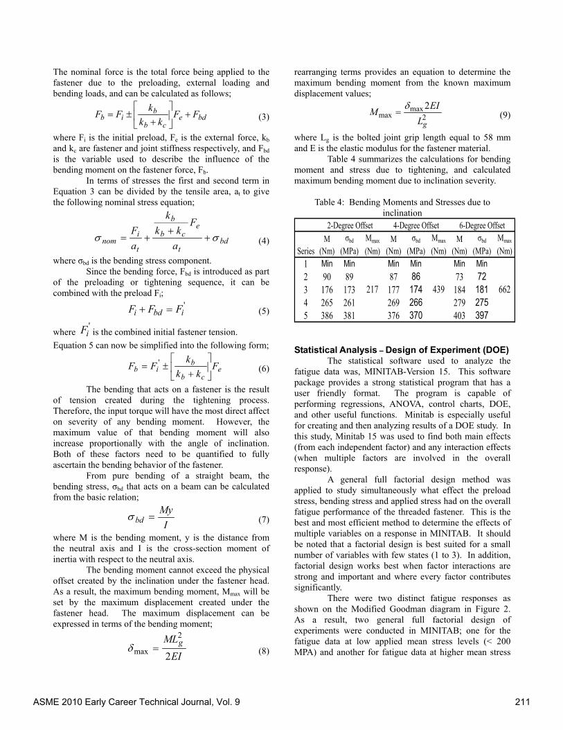
The results of the 1st DOE can be summarized in the two plots shown in Figures 8 and 9 respectively. Figure 8 is a main effects plot which plots the means for each factor level. The reference line (horizontal) is the overall mean of the response (cycle) data. The plot provides a good visualization of effect magnitude for each of the three factors analyzed in this experiment. Figure 8 shows that the applied cyclic load, mean stress and bending stress all have an effect on the number of cycles to failure at low applied mean stress levels (≤ 200 MPa). All three plots have a negative slope indicating each variable had a negative effect on cycles to failure. The applied cyclic load had the greatest effect (steepest slope) while the mean and bending stresses have a lesser but similar effect. Thus all three factors had a negative effect on cycles to failure in fasteners with low mean stress levels.

Figure 8: Main effects plot from 1st DOE

Another means of visualizing factor effects is through three-dimensional (3D) surface models. Surface models are best suited for an analysis involving three factors one each for the x, y, and z axes. Figure 9 is the 3D response

500000040000003000000200000010000000

500

400

300

200

100

0

Cycles

Sigm

a_m

Scatterplot of Sigma_m vs Cycles

500000040000003000000200000010000000

250

225

200

175

150

125

100

Cycles

F_e

Scatterplot of F_e vs Cycles

500000040000003000000200000010000000

300

250

200

150

100

50

0

Cycles

Sigm

a_bd

Scatterplot of Sigma_bd vs Cycles

23186

3000000

2000000

1000000

04700

2750

3000000

2000000

1000000

0

F_e

Mea

n

Sigma_m

Sigma_bd

Main Effects Plot for CyclesData Means


surface for those fasteners having a low applied mean stress level.

Figure 9: Surface plot from 1st DOE

DOE – HIGH APPLIED MEAN STRESS LEVELS Figures 10-12 show the number of cycles at failure versus each stress variable from the high mean stress level (> 200 MPa) fatigue results. Figure 10 is a scatter plot showing mean stress (preload) versus cycles to failure.

Figure 10: Scatter plot mean stress vs failure cycles

Figure 11 is a scatter plot showing cycles to failure versus the applied cyclic load.

Figure 11: Scatter plot cyclic load vs failure cycles

Figure 12 is a scatter plot showing cycles to failure versus bending stress.

Figure 12: Scatter plot bending stress vs failure cycles

The results of the 2nd DOE have been summarized in the two plots shown in Figure 13 and 14 respectively. Figure 13 is the main effects plot for the applied cyclic load, mean stress and bending stress. Figure 14 is the 3D surface plot of these three factors. Figure 13 shows a much different response of failure cycles to the three main factors of applied cyclic load, mean stress and bending stress. Only one plot, the applied cyclic load has a steep, negative slope. This makes the applied cyclic load the only factor that had a significant, negative effect on cycles to failure. The mean and bending stresses, have relatively flat lines that show a slight increase in slope. Thus, there is little effect of either the mean or bending stress on the cycles to failure in those fasteners with a high applied mean stress level (> 200 MPa).

100

150

200

0100

200

250

150

0200

300

150

450

0

F_e

Sigma_m

Sigma_bd

Surface Plot of F_e vs Sigma_m, Sigma_bd


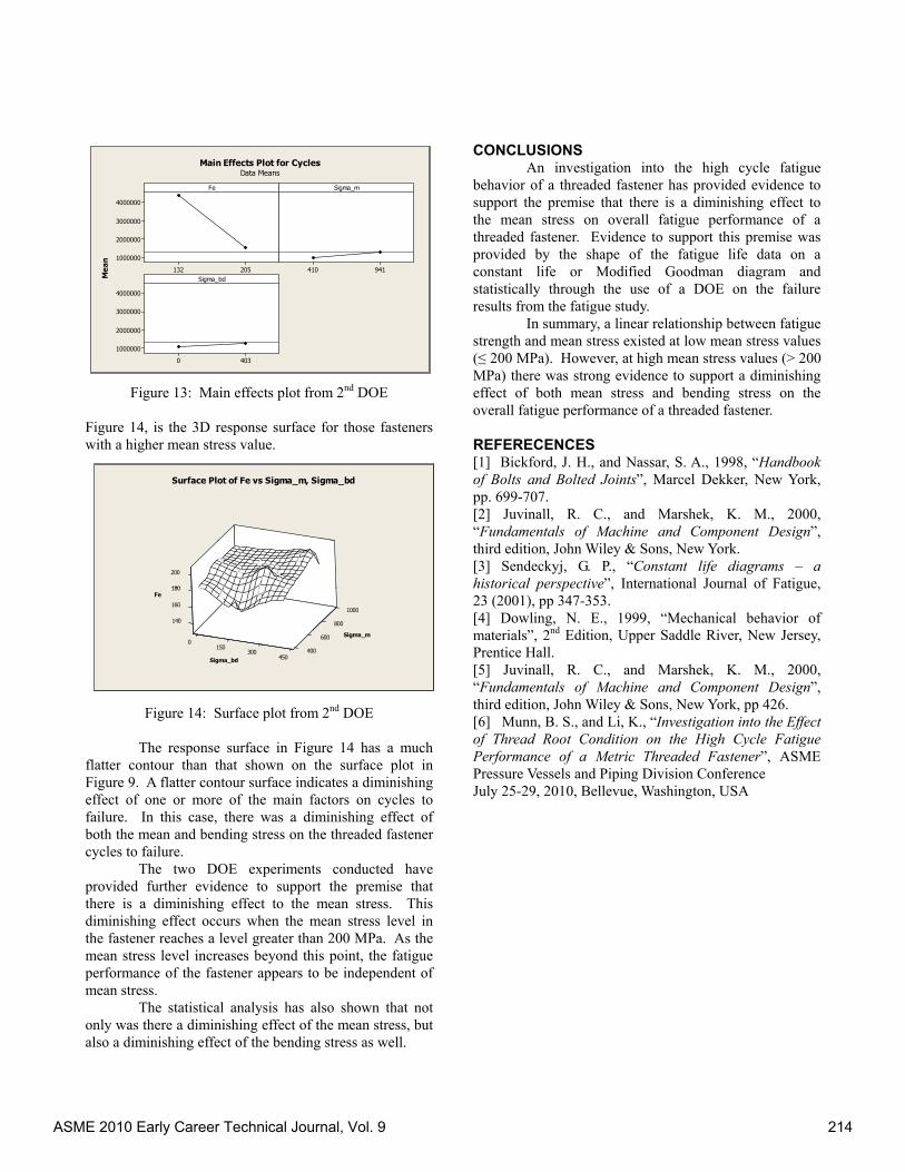
Figure 13: Main effects plot from 2nd DOE

Figure 14, is the 3D response surface for those fasteners with a higher mean stress value.

Figure 14: Surface plot from 2nd DOE

The response surface in Figure 14 has a much flatter contour than that shown on the surface plot in Figure 9. A flatter contour surface indicates a diminishing effect of one or more of the main factors on cycles to failure. In this case, there was a diminishing effect of both the mean and bending stress on the threaded fastener cycles to failure. The two DOE experiments conducted have provided further evidence to support the premise that there is a diminishing effect to the mean stress. This diminishing effect occurs when the mean stress level in the fastener reaches a level greater than 200 MPa. As the mean stress level increases beyond this point, the fatigue performance of the fastener appears to be independent of mean stress. The statistical analysis has also shown that not only was there a diminishing effect of the mean stress, but also a diminishing effect of the bending stress as well.

CONCLUSIONS An investigation into the high cycle fatigue behavior of a threaded fastener has provided evidence to support the premise that there is a diminishing effect to the mean stress on overall fatigue performance of a threaded fastener. Evidence to support this premise was provided by the shape of the fatigue life data on a constant life or Modified Goodman diagram and statistically through the use of a DOE on the failure results from the fatigue study. In summary, a linear relationship between fatigue strength and mean stress existed at low mean stress values (≤ 200 MPa). However, at high mean stress values (> 200 MPa) there was strong evidence to support a diminishing effect of both mean stress and bending stress on the overall fatigue performance of a threaded fastener. REFERECENCES [1] Bickford, J. H., and Nassar, S. A., 1998, “Handbook of Bolts and Bolted Joints”, Marcel Dekker, New York, pp. 699-707. [2] Juvinall, R. C., and Marshek, K. M., 2000, “Fundamentals of Machine and Component Design”, third edition, John Wiley & Sons, New York. [3] Sendeckyj, G. P., “Constant life diagrams – a historical perspective”, International Journal of Fatigue, 23 (2001), pp 347-353. [4] Dowling, N. E., 1999, “Mechanical behavior of materials”, 2nd Edition, Upper Saddle River, New Jersey, Prentice Hall. [5] Juvinall, R. C., and Marshek, K. M., 2000, “Fundamentals of Machine and Component Design”, third edition, John Wiley & Sons, New York, pp 426. [6] Munn, B. S., and Li, K., “Investigation into the Effect of Thread Root Condition on the High Cycle Fatigue Performance of a Metric Threaded Fastener”, ASME Pressure Vessels and Piping Division Conference July 25-29, 2010, Bellevue, Washington, USA

205132

4000000

3000000

2000000

1000000

941410

4030

4000000

3000000

2000000

1000000

Fe

Mea

n

Sigma_m

Sigma_bd

Main Effects Plot for CyclesData Means

140

160

180

0150

300

180

200

1000

800

600

400450

Fe

Sigma_m

Sigma_bd

Surface Plot of Fe vs Sigma_m, Sigma_bd


ASME Early Career Technical Journal

2010 ASME Early Career Technical Conference, ASME ECTC October 1 – 2, Atlanta, Georgia USA

COMPUTER-AIDED PRODUCT AND PROCESS DEVELOPMENT OF LACE BRAIDED COMPOSITES

David J. Branscomb, M.Sc. Department of Polymer and Fiber Engineering

Auburn University Auburn, Alabama, USA

David G. Beale, Ph.D. Department of Mechanical Engineering


Royall M. Broughton Jr., Ph.D. Department of Polymer and

Fiber Engineering Auburn University

Auburn, Alabama, USA

ABSTRACT Braided fabrics are often used in the production of structural composites. Among many favorable attributes, braided structures can be tailored to meet design criteria by controlling the yarn geometry. A specialized type of braiding machine where each yarn is individually controlled is known as a lace braiding machine. A computer aided engineering (CAE) process is developed in order to utilize the unique ability of lace braiding machines and determine how well lace braided fabric will perform as a composite pre-form. Braided topology is modeled using computer aided design (CAD) software. Finite element analysis (FEA) is performed on three dimensional (3-D) models to determine structural performance. An example of optimized geometry is presented. A manufacturing technique capable of infusing yarns with polymeric resin and curing to produce rigid structures is developed. Structures are evaluated using mechanical testing equipment. Some envisioned structures are presented. A number of challenges must be addressed to develop a knowledge based engineering (KBE) process to enable the structural design of braided lace composites. Solutions to these challenges are presented and will be the basis for evaluating the performance and manufacture of lace braided composites.

INTRODUCTION Composite materials are often made from fabric pre-forms constructed of high-strength fibers. Pre-forms serve as the primary structural reinforcement in a composite. Braided fabric pre-forms are produced by interlacing yarns in such a way that a continuous, conformable material is formed. As such, braided pre-forms can be manufactured to final design geometry. Braided pre-forms exhibit many favorable attributes

such as low cost, complex shape capability, seamless coverage, and designable material properties. Conventional braiding machines are limited to specific architectures. However, lace braiding machines control the individual yarn positions by electromagnetic-mechanical actuation, permitting the manufacture of intricate fabrics with endless architecture possibilities. In industry, lace braiding machines are used to make fancy garments, such as lingerie. This research utilizes lace technology to orient yarns and create truss pre-forms in flat, polygon, or cylindrical cross section. Subsequent saturation with polymeric resin and autoclave curing produces a composite truss. It is known that a truss provides higher strength at lower weight than a solid beam, therefore we expect the open, versatile nature of lace braided composites, to provide a higher strength-to-weight ratio than a solid composite structure. Lace technology is primarily utilized by fashion designers, thus design is an art based on tradition and experience; the design tools available are insufficient for engineering analysis. We have developed a computer aided engineering (CAE) toolset based on translating the fundamental motions of the lace braiding machine into the resulting braided structure while simultaneously supplying the instructions required by the machine to produce the actual braid. The number of yarns, dimensions, and required machine steps are inputs. Cartesian coordinates of each yarn are generated for a given design. Yarn curvature is approximated using B-Spline interpolation. A 3D model representative of yarn kinematics with dimensional accuracy and scalability is the result. Future work will involve investigating virtual lace braided models to satisfy a desired performance criteria. 3-D models are exported as stereolithography files or reconstructed in CAD and easily


imported to finite element analysis (FEA) software. Topological optimizations will be investigated using FEA to design a lace braided structure where the yarns follow regions of maximum principal stress, leaving reinforced areas surrounded by open area where stress is minimal. The work of this paper involves developing a specific KBE toolset in order to realize the potential of implementing pattern control within a braided structure to produce optimized, minimal weight structural composites. Figure 1 demonstrates the process schematic for the proposed computer aided engineering and evaluation of lace braided composites.

Figure 1. Knowledge Based Engineering Process

Schematic

MOTIVATION The major thrust of the proposed work was the

evaluation and use of braided textile pre-forms for the manufacture of engineered fiber reinforced composite structures. Particular emphasis was placed on using open-lace structures for minimum weight composites. Solid composite materials have been tested, proven, and are currently used by most engineering industries. However, it is not known exactly how well or to what extent lace structures will perform as pre-forms for structural composites. This work supports developing a tool for designing, analyzing, and manufacturing composites from lace pre-forms.

A lace braiding machine is believed to be suited for the manufacture of the proposed minimal weight composites. A lace braiding machine is designed to create open structures and with the substitution of large high strength yarns such as Kevlar(R), Vectran(R), and carbon fiber, it is thought that the structures might be suitable for use as planar and 3-D space trusses.

RELEVANCE TO COMPOSITES INDUSTRY

Figure 1 illustrates the KBE tool developed specifically for the design, evaluation, and manufacture lace

braided pre-forms. This tool is relevant to the composites industry, as well as a plethora of related industries, for several reasons. First, the computer model is specific to lace braiding machines and therefore the simulation is representative of the design. By analyzing the fundamental motions of lace machines to develop the framework from which lace designs are derived, a mathematical description is developed to provide design intuition. Second, a significant learning curve is required to design lace. The design tools being developed will be useful to provide the intuition needed to design effectively. The following excerpt from Imitations of handmade-lace by machinery exemplifies the significance of the lace design experience, “The preliminary work of designing and drafting is difficult and requires years of training for proficiency to be obtained [1].”

MAJOR CHALLENGES OF MANUFACTURING AND MODELING Many challenges must be overcome to utilize lace braiding technology to produce predictable composite materials. Some challenges which must be addressed in order to use lace braiding for producing engineered composite structures are listed in Figure 2.

Figure 2 Challenges which must be solved for lace

braided composites to become an engineering technology

The first challenge is understanding lace braiding technology. Although lace machines have been in use for many years, the published literature is scarce. The industry is esoteric and specialized. Lace braiding machines have specific challenges not encountered with conventional braiding machines, which must be understood and addressed to use the machine effectively. Until the composites industry acquires the expertise required to design lace, this problem will not be resolved.


Addressing some specific design challenges: Once a 3-D model is generated it can be converted to a stereolithograph file. Ideally this file will be used directly with finite element software. Additionally, Cartesian coordinates for individual yarns can be imported to CAD as well as other commercially available software for further analysis. In order to utilize the computer aided design tools presented effectively, these simulation and analysis related issues must be resolved:

• Determine constitutive material properties • Modeling the interlacing points or “joints”

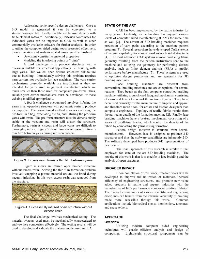
A third challenge is to produce structures with a thickness suitable for structural applications, i.e. braiding with large yarns. Thin walled, open fibrous structures risk failure due to buckling. Immediately solving this problem requires yarn carriers not available for lace machines. The yarn carrier mechanisms presently available are insufficient as they are intended for yarns used in garment manufacture which are much smaller than those used for composite pre-forms. Thus, suitable yarn carrier mechanisms must be developed or those existing modified appropriately. A fourth challenge encountered involves infusing the yarns in an open-lace structure with polymeric resin to produce a composite. The conventional method involves enclosing the pre-form in a bag, evacuating the air, and infusing the pre-form yarns with resin. The pre-form structure must be dimensionally stable or the vacuum and resin will distort the structure. Furthermore, resin is viscous and large yarns are difficult to thoroughly infuse. Figure 3 shows how excess resin can form a thin film between yarns during infusion process.

Figure 3. Excess resin forms a thin film between yarns.

Figure 4 shows an infused open braided structure without excess resin. Solving the thin film formation problem involved wrapping a porous material around the braid during vacuum infusion. In this way, excess resin was removed from the structure.

Figure 4. Successfully infused open structure without

excess resin.

The final challenge involves mechanical testing. The material systems used must be mechanically characterized to analyze lace composites effectively. The testing results will be used to develop and validate the material model used in FEA.

STATE OF THE ART CAE has been implemented by the textile industry for many years. Certainly, textile braiding has enjoyed various levels of computer aided manufacturing (CAM) for some time as well [2]. The advent of 3-D braiding machines required prediction of yarn paths according to the machine pattern program [3]. Several researchers have developed CAE systems of varying capability for conventional rotary braided structures [4]. The most advanced CAE systems involve producing fabric geometry resulting from the pattern instructions sent to the machine and utilizing the geometry for performing desired analysis, such as finite element analysis (FEA) to predict performance before manufacture [5]. These systems are used to optimize design parameters and are generally for 3D braiding machines. Lace braiding machines are different from conventional braiding machines and are exceptional for several reasons. They began as the first computer controlled braiding machine, utilizing a punch card Jacquard mechanism consisting of cams and levers to control the motion of yarns. They have been used primarily for the manufacture of lingerie and apparel and therefore more a tool for artists and fashion designers than composite engineers. Topology of textile fabrics results from the particular details of the formation machine [2]. Finally, lace braiding machines have a beat-up mechanism, consisting of a series of oscillating blades, which control the density of the fabric by compacting the yarns during formation. Pattern design software is available from several manufacturers. However, lace is designed to produce 2-D structures and thus the software capabilities are inherently 2-D. The software developed here produces 3-D representations of lace braids. The CAE approach of this research is similar to that employed for state of the art 3-D braiding machines. The novelty of this work is that it is specific to lace braiding and the analysis of open structures.

BROADER IMPACT Upon completion of this work, research tools will be developed to improve the utilization of materials, increase efficiency of engineering structures, and promote new value added products in textile and apparel industries with the manufacture of high performance composite pre-form fabrics. The research communities of various scientific and engineering disciplines can benefit from the intrinsic versatility of braiding made more accessible through this work. Common applications include biomedical stents, biomicmicry, antennas, and space tethers.

APPROACH Overview Utilizing modern computer aided engineering techniques will enable efficient analysis and design of composites. Lightweight structural components can be


achieved by strategic positioning of reinforcing fibers along the principal stress directions, allowing the structure to maintain a high strength-to-weight ratio. Figure 4 shows one recent commercially available example of open truss composite structures similar to what is envisioned.

Figure 4. Open Truss Composite Bicycle Frame [6]

Modeling of Yarns The fundamental structural elements of composite pre-forms are yarns. Pre-form geometry can be determined by the yarn cross-section and center-lines of the constituent yarns, as well as mold or mandrel geometry. The geometry of individual yarns may also vary, depending on the pattern and other processing parameters. The basis for reliable engineering and prediction of lace composite properties is derived from realistic representation of fabric geometry. The advantage of using a generative model along with parametric input, is that realistic geometry can be adjusted for a desired yarn system. The basic idea of this modeling technique is that each yarn is created by sweeping a cross-section along a 3-D path and then assembling the yarns to make the structure. Yarns are generated and can be adjusted with B-Spline interpolation. B-Splines provide a good ability to represent complex paths [7]. The path and cross-section of the yarn may be adjusted to fit observation. Figure 5 illustrates how yarn paths can be smoothed and adjusted to improve accuracy. The CAE capabilities of the proposed system are illustrated in Figure(s) 1,5,7-10.

Figure 5 Yarn path without B-Spline interpolation (top)

and yarn path with B-Spline interpolation (Bottom)

Import to CAE Software After a braided structure is generated, the 3-D model can be exported as a stereolithography file or as XYZ data and reconstructed in CAD/CAE software. In this way, the full design capacity of commercially available software can be employed. Lace braided structures are often complex and cannot be represented with small conventional unit cell based mechanics analysis methods. However, importing CAD geometry is common in finite element analysis software; thus, if accurate geometry can be generated it can be used accordingly. The design tools presented in this work are capable of accurate geometry generation. FEA: Initial Basis of Optimization As an example of how the presented CAE system can be used to perform topological optimizations, a cylinder has been analyzed to represent a particular braided structure and loading condition and the result is shown in Figure 6.

Figure 6. Example Braided Tube FEA Stress Distribution

Low Stress Regions

Higher Stress Regions


Figure 7. Topological optimization first attempt based on

the stress pattern observed in Figure 6.

Considering Figure 6 and 7: The stress distribution of Figure 6 is used to design an approximate lace structure. Figure 7 illustrates how braided topology can be tailored considering the stress distribution. An lace braided cylinder is designed where the yarns populate regions of maximum principal stress, leaving reinforced areas surrounded by open area where expected stress is minimal. It is envisioned that that the set of design tools developed during this work will provide the necessary insight to produce minimal weight composite structures that utilize material more efficiently. Manufacturing

Once a particular design has been created, the specific manufacturing instructions are sent to the lace braiding machine to produced the pre-form. A Vacuum assisted resin transfer molding technique is employed to infuse the pre-form yarns with a polymeric resin. The resin saturated pre-form is cured in an autoclave to produce the rigid composite structure. Evaluation of Structures

Structural materials for whatever application must withstand tension, compression, bending, torsion, and perhaps impact loading. Once a design has been manufactured, the structural integrity will be tested by various measurement and instrumentation techniques. Preliminary evaluation of tension, compression, and flexion will be performed utilizing mechanical testing equipment. The measured physical properties will be used to develop an appropriate material model and incorporated in FEA predictions.

RESULTS The result of the computer aided engineering toolset presented produces virtual lace braided models that can be used to improve the design process. The toolset is capable of generating realistic CAD models, representative of the actual

manufacturing process and will be used to optimize a desired performance criteria. The designer can experiment graphically with endless possible architectures, while simultaneously producing the instructions required by the machine to produce the actual braid. Conventional pre-form architectures are also represented (Figures 8-9). Figure 8 is a virtual triaxial diamond braid model and can be produced using a lace braiding machine. Figure 9 demonstrates how CAD models created with this system can be imported in commercially available FEA software and analysis performed. .

Figure 8. Triaxial Diamond Braid Model

Figure 9. Preliminary FEA of Lace Composite

Low Stress Regions

Higher Stress Regions


Figure 10 Example Pre-form Architectures.

CONCLUSIONS Applying advanced design and manufacturing techniques enables the precise placement of yarns to maximize the structural performance of composite materials. Utilizing computer aided engineering techniques enables efficient analysis and design of composites. The work presented in this paper addresses important challenges of engineering design of braided lace composites. It also allows the construction of computer generated fabric pre-forms in a single manufacturing step. The result of this work is the development of a CAE based approach capable of producing 3-D CAD models, evaluating their performance, optimization, and manufacture of lace braided composite structures.

ACKNOWLEDGEMENTS The authors would like to thank the Alabama

Space Grant Consortium NASA Training Grant #NNG05GE80H for supporting this work. The authors would also like to thank David Jackson for his excellent efforts in this project. The Auburn University Department of Polymer and Fiber Engineering Braiding and Composites Research Laboratory provided necessary equipment and technical support.

REFERENCES

[1] Imitations of Hand-Made Lace by Machinery, Part I, Middleton, George. The Bulletin of the Needle and Bobbin Club, Vol. 22 (1938) [2]Adanur, S. (1995). WELLINGTON SEARS HANDBOOK OF INDUSTRIAL TEXTILES. Lancaster: Technomic Publishing Company, Inc. [3]Anthony K. Pickett, J. S. (2009). Braiding Simulation and Prediction of Mechanical Properties. Applied Composite Materials , 345-364. [4] Mei-Zhong Zhang, H.-J. L. (2007). Automatically generated geometric description of 3D braided rectangle preform. Computational Materials Science , 836-841.

[5] M Schneider, A. P. (2000). A NEW ROTARY BRAIDING MACHINE AND CAE PROCEDURES TO PRODUCE EFFICIENT 3D BRAIDED TEXTILES FOR COMPOSITES. 45th International SAMPE Symposium (p. 11). Long Beach: SAMPE. [6] http://www.delta7bikes.com/delta7-bikes.htm [7]Bjourn Van Den Broucke, K. D. (2007). MULTILEVEL MODELLING OF MECHANICAL PROPERTIES OF TEXTILE COMPOSITES: ITOOL PROJECT. SAMPE Europe International Conference 2007 Paris (pp. 175-180). Paris: SAMPE.


ASME Early Career Technical Journal 2010 ASME Early Career Technical Conference, ASME ECTC

October 1-2, 2010, Atlanta, Georgia, USA

DAMAGE EVALUATION OF BRAIDED KEVLAR®/CARBON/EPOXY COMPOSITE BEAMS IN THREE POINT BENDING WITH INFRARED THERMOGRAPHY

David J. Branscomb Department of Mechanical Engineering


Idris Cerkez Department of Polymer and Fiber Engineering


ABSTRACT A braided composite beam is tested in three-point

bending. Infrared images are generated during the deformation and captured. Custom image processing algorithms are developed to capture infrared events during three-point bending of braided composite material. Image processing was utilized to compare observed damage to theoretical models, with what appears to be good results. The results suggest that obsolete IR thermography equipment can be revitalized and used to monitor Kevlar®-Carbon composite material damage. Three-point bending testing in conjunction with infrared thermography can prove to be an effective method for damage evaluation of composite material. INTRODUCTION

Polymer composites have shown promise as light weight engineering designer materials. As such, it is necessary to develop a quantitative analysis and methodology for assessing the safety and reliability of using polymer composites in various applications. Baer, Van Paepegem and Degrieck investigated the feasibility of three-point bending data for the validation of fatique models for thin fiber-reinforced composites and found that 3-point bending is not ideal [2]. However, the author of this work believes that Three-point bending testing in conjunction with infrared thermography can prove to be an effective method for damage evaluation of composite materials. Especially in aerospace applications, structural polymer composites require fatigue reliability in different environments and loading conditions. Hansen investigated tensile fatigue damage in woven polymer composites [5]. Degradation by fatigue of composites is a

complex phenomenon, involving several influential factors in the damage of material.

The inherent nature of composites is that of inhomogeneous microstructure with disparate constituent properties. Differences in stiffness and strength result in complex damage development and failure processes, including various fracture modes. Previously researchers performed tensile tests of triaxial braided composites along with optical surface strain and acoustic emission measurements; the resulting damage was observed using X-ray and microscopy techniques and found to develop as intra-yarn cracking and as local inter-yarn delamination [3]. Researchers utilized ultrasonic physics, as a way to estimate elastic moduli, by measuring the velocity of elastic wave propagation through a medium [7].

Thermography

Thermography is also known as thermal inspection or infrared (IR) imaging is one of the most common nondestructive testing (NDT) methods, and it is being used more as the technology improves and users begin to realize the true potential of this testing method (Thermal-infrared). Thermography is a noncontact, noninvasive non destructive testing (NDT) method that can be used with various surface geometries and conditions. Thermography is ideal for in situ evaluation and particularly valuable where accessibility is limited.

Toubal developed a thermography technique that has been used to study the evolution of temperature on the specimen surface. This system can characterize degradation by fatigue of composite material [6]. An important aspect of thermography is that it utilizes the relationships between the materials temperature evolution and mechanical behavior according the


thermoelastic, thermoplastic, and heat conduction effects [1]. The thermoelastic effect contributes to the material temperature oscillation with stress change. The thermoplastic effect contributes to the material mean temperature change. The heat conduction effect contributes to the material mean temperature change.

A typical NDT application of thermography involves using imaging techniques to evaluate the thermal signatures of test objects. The test object is excited in some way and the resulting infrared emission provides an indication of the material state for the given excitation. In the case of this experiment, mechanical deformation produces energy dissipation throughout the specimen. The thermal signatures are used to evaluate the onset and propagation of damage, in this case fiber-matrix break and delamination. The practices employed in this experiment involve older IR thermographic technologies where the user views thermographic NDT data as a movie where anomalous hot spots which might be indicative of occurring damage are seen. This method has been proven to be effective in some applications, but is entirely qualitative, relying on the intuition of the inspector (Shepard, Understanding Flash Thermography, 2006).

For this experiment modern PC based programming and image analysis has been merged to increase functionality of the IR camera. So in this way, the work presented here provides a framework for developing a more quantitative approach that can be coupled to the previous qualitative IR system. By processing the data with dedicated image analysis algorithms enables the detection and measurement of features that are not detectable by direct viewing of the camera.

Emissivity is the ratio of the infrared energy radiated by an object at a given temperature to the energy emitted by a blackbody at the same temperature (Frederic Jacoba, 2003). Polymer composites have sufficiently high emissivity values to enable thermographic testing with minimal preparation [11]. Additionally, Polymer composites typically have thermal diffusivity properties suitable for thermographic NDT. Based on published values for emissivity and diffusivity, Kevlar-Carbon-Epoxy composites used in this experiment are suitable for thermographic testing.

Thermography is generally classified as either active or passive modes. The conventional understanding of active involves using an external thermal exciter (Rajan, 2009). Passive thermography is the opposite, with no thermal exciter. The testing performed in this experiment is passive, but could possibly considered active, as the excitation comes from the mechanical loading. Passive NDT techniques are often utilized while the specimen is at steady state conditions.

Three Point Bending Three point bending is a flexural test that provides

information regarding bulk material properties. These properties include bending modulus of elasticity and flexural

stress and flexural strain. The flexural stress-strain response is shown in Figure 1 for a representative composite specimen.

Figure 1. Midspan deflection versus load (x axis is cm, y axis KN)

(Prewo, 1980)

The disadvantages of three point bending are sensitivity to specimen geometry, loading and strain rate. However, ease of specimen preparation is a primary advantage over other testing procedures. Three point bending is the standard test for basic bending and flexural analysis.

The three-point bending process is simple. Place the specimen across the roller supports. The distance between supports is dictated by specimen geometry and typically specified for a given standard. The specimen is loaded in the middle of the roller supports, see Figure 2. A modification of any of these conditions will alter the bend and should be kept in mind during experiment. For rectangular specimen in three-point bending, the following relationship exists.

Where

• σ is the flexural stress

• F is the load (force) at the fracture point

• L is the length of the support span

• b is width

• d is thickness

Figure 2. Three-point bending setup


Manufacture Of Composite Material The composite beams are fabricated using over-

braiding (See Figure 3). Polyvinyl alcohol (PVA) is applied to an aluminum mandrel as a release agent. Sixteen Kevlar® yarns are braided over the aluminum mandrel to form an open inner layer with approximately seventy percent coverage. Next, Epoxy pre-impregnated carbon unidirectional tape is manually placed on the top of the inner layer, following an outer layer of 16 additional Kevlar® yarns. The initial Kevlar® layer provides support for the carbon and the outer layer encases the carbon. Vacuum assisted resin transfer molding technique is employed to infuse the yarns both on top and underneath the carbon with polyester resin. Infrared heating lamps heat the sample to promote infusion and polymerization. The composite is heated in a convection oven to promote secondary curing for 12 hours. Finally, the PLA is dissolved and the mandrel is removed to produce the final form composite. The beam is cut to length for testing. The test specimen dimensions are 12.7 mm in width, 28.5 mm in height, 0.8 mm in thickness, and 95.25 mm in length. The test specimen has a mass of 5 grams.

Figure 3. Manufacturing Steps

EXPERIMENTAL SETUP

An Instron model 5565, mechanical testing machine was used during this experiment. Infrared images are produced using camera system shown in Figure 4. LabVIEW is used for image acquisition on a PC with frame grabber.

Figure 4. Infrared Image Analysis

Figure 5. Three point bending setup

Image Processing

A personal computer (PC), equipped with a frame grabber, was used. The IR camera system outputs video in NTSC format of 30 frames per second (fps). A simple data acquisition program was written, using National Instruments LabVIEW, to capture the video data and parse images. The resulting images are noisy and require some post processing to improve the information of interest. Image processing is performed according to the schematic presented in Figure 6. The image includes extraneous information including some constant noise defects due to poor connection. A region of interest (ROI) is selected to minimize computations and improve processing efficiency. All pixels outside the ROI are masked from subsequent processing. Color images, Red Green Blue (RGB) are constructed of 3 color planes, red, blue, and green. For this analysis the green plane is removed, further simplifying the image processing requirements and rendering a grayscale image. Morphological processes involve manipulating the shape of pixels in the image. The pixels in the ROI are dilated by a 5 by 5 matrix to increase visibility. Finally, the resulting image pixels above a defined threshold are shown. The resulting image is seen in Figure 6. Processing the data with dedicated image analysis algorithms enables the detection and measurement of features that are not detectable by direct viewing of the camera. The custom image processing system developed here is a step towards adding a quantitative component to the previous qualitative IR system.

Figure 6. Image processing algorithm flow chart


EXPERIMENTAL RESULTS

Control Specimen First, three-point bending of braided composite beam

is performed to provide baseline information regarding the behavior under quasi static loading. The cross head speed is 1 mm/min and the results are given in Figure 7

Figure 4. Three-point bending of control braided composite

The yellow circles in Figure 7 show how load is

redistributed to remaining undamaged fibers. The stress in one or more fibers increases until break and the load precipitously drops briefly and then increases again as surrounding yarns carry the load. This phenomenon occurs several times and is related to the inherent nature of braid topology to redistribute the load to the remaining fibers. The occurrence of similar events can be inferred from Figure 8.

Three Point Bending Of Braided Composite Observed With IR Camera

A dynamic test is performed to evaluate how bending strength and stiffness might be affected by loading and to observe corresponding infrared events. Fiber/yarn/matrix/delaminations occur similar to those encountered in Figure 7 within the initial load-displacement curve. During the three point bending test, the composite beam began to contort and eventually fell on its side, which explains the right side of Figure 8. It is interesting to note that region II captures the falling of the composite and the now transversely loaded specimen also supports a considerable load.

Figure 5. Three-point bending and contorting of composite

The IR thermographic bending test occurs as follows. After loading the composite, it is held sufficient amount of time to allow the specimen to reach thermal equilibrium. Then the three point bending loading and image acquisition occur simultaneously. The first detected IR event is seen in Figure 9.

Figure 6. Initial IR image

Damage of Composite The braided composite is loaded until it eventually contorts and falls on its widest side. The damage of the yarns and matrix appears as the white surface detail of Figure 10.


Figure 7. Composite damage due to delamination and matrix

cracking propagated in a triangular area Comparison to theory

Figure 11 illustrates the damage state of the composite as damage propagation has occurred approximately halfway through the structure.

Figure 8. Composite Damage captured with IR Thermography

Figure 9 Theoretical finite element damage model[12]

Figure 10. Damage propagation after image processing

CONCLUSION Infrared imaging techniques can be used to monitor

Kevlar®-Carbon braided composites. The work presented here involved developing custom image processing algorithms to capture infrared events during three-point bending of braided composite material. Image processing was utilized to compare observed damage to theoretical models, with what appears to be good results. These results suggest that obsolete IR thermography equipment can be revitalized and used to monitor

Kevlar®-Carbon composite materials. Finally, three-point bending testing in conjunction with infrared thermography can prove to be an effective method for damage evaluation of composite material.

FUTURE WORK A continuation of this study should be done to quantify

the flexural material properties such as bending modulus. Finite element analysis models should be developed to confirm degradation according to the unique composite constituents manufactured here. Acoustic emission events could correlate fiber/yarn/matrix break occurrence on stress-strain diagram and correlated to IR thermographic events. ACKNOWLEDGEMENT

The authors would like to thank the Alabama Space Grant Consortium NASA Training Grant #NNG05GE80H for supporting this work.

REFERENCES [1] B. Yang, P. L. (2003). Thermography: A New Nondestructive Evaluation Method in Fatigue Damage. JOM: The Member Journal of TMS . [2] Baere, P. D. (2008). On the Feasibility of a Three-Point Bending Setup for the Validation of (Fatique) Damage Models for Thin Composites Laminates. Polymer Composites , 1067-1076. [3] Dmitry S. Ivanov, Fabien Baudry, Björn Van Den Broucke, Stepan V. Lomov, Hang Xie, Ignaas Verpoest. (2009). Failure analysis of triaxial braided composite. Composites Science and Technology , 1372-1380. [4] Frederic Jacoba, F. P. (2003). Comparison of land surface emissivity and radiometric temperature derived from MODIS and ASTER sensors. Remote Sensing of Environment , 137-152. [5] Hansen, U. (1999). Damage Development in Woven Fabric Composites During Tension-Tension Fatigue. Journal of Composite Materials , 614-639. [6] Lotfi Toubal, M. K. (2006). Damage evolution and infrared thermography in woven. International Journal of Fatigue , 1867-1872. [7] Nesvijski. (1999). Some aspects of ultrasonic testing of composites. Composite Structures , 151-155. [8] Prewo. (1980). The Importance of Fibres in Achieving Impact Tolerant Composites. Philosophical Transactions of the Royal Society of London. Series A, Mathematical and Physical Sciences , 551-558. [9] Rajan, P. (2009). Infrared Thermography. Auburn University: Department of Mechanical Engineering. [10] Shepard. (2007, July). Thermography of composites. Materials Evaluation , pp. 690-696. [11] Shepard. (2006, May). Understanding Flash Thermography. Materials Evaluation , pp. 460-464. [12] http://mech.fsv.cvut.cz/~milan/videos.html


A NEW SINGLE TRANSIENT TECHNIQUE TO MEASURE

FILM COOLING PERFORMANCE: GAS TURBINE APPLICATION

Mohamed G. Ghorab, PhD Mechanical Engineering Alexandria University Montreal, QC, Canada

ABSTRACT

This paper presents in detail a new single transient experimental technique and methodology for measuring film cooling effectiveness and heat transfer coefficient. During the present experimental test, the mainstream at supply temperature and the heated secondary flow were suddenly directed over the measured surface. Thermochromic Liquid Crystal (TLC) was used to measure the transient surface temperatures. A nonlinear least square regression method (LSQ) was used to calculate the two unknown parameters with minimize the experimental error. The film cooling effectiveness and heat transfer coefficient for a circular hole were investigated at blowing ratio of 0.5 and 1.0 then the results were compared with other published data for different transient and steady state techniques. The results showed that the current transient experimental technique and methodology provided a good agreement with published data. Therefore, the current experimental technique and methodology can be utilized for future transient experimental test for gas turbine applications. NOMENCLATURE Symbols Br blowing ratio (ρjVj/ρmUm) Cp specific heat (J/kg.K) d hydraulic diameter of film hole (m) Dh hydraulic diameter of main duct (m) Dr density ratio (ρj/ρm) h heat transfer coefficient (W/m2.K) Hue hue color component I momentum flux (ρjVj

2/ρmUm 2)

k thermal conductivity of plate (W/m.K) p film hole pitch (m) q heat transfer flux (W/m2) Re Reynolds number (ρUmDh/μ) T temperature (K) t time(sec) Tw average wall temperature (K) Um normal main stream velocity in x direction (m/s) Vj injection flow velocity (m/s) x,y,z coordinates

Greek symbols α thermal diffusivity (m2/s), = (k/ρCp) ε least square error η local film cooling effectiveness = (Tf-Tm)/ (Tj-Tm) . ηav span-wise averaged film cooling effectiveness =

(Tw-Tm)/ (Tj- Tm). ρ density (kg/m3) τ color change time (sec) Subscripts and superscripts 1,2 first and second time step av average aw adiabatic condition c centerline f film cooling i initial IG initial guess j jet m main stream o without film s solid w wall conditions Abbreviations LSQ least square regression RGB red, green, blue TIFF tagged image file format TLC thermochromic liquid crystal

1. INTRODUCTION Film cooling measurement includes three

temperature systems namely: the injection temperature, the mainstream temperature and the wall temperature. Two equations are needed in order to calculate film cooling effectiveness and heat transfer coefficient using the three-temperature system at every measurement location over the entire area. Therefore, two similar transient runs are needed to generate two different sets of conditions, which are dependent on the experimental setup. There are two popular transient techniques. The frst technique is to heat the mainstream while the secondary flow is kept at the ambient temperature. During the experimental test, the heated mainstream and the secondary flow are suddenly directed over the measured surfaces. In addition, the mainstream and the injection flow are heated and suddenly imposed over the measured


surface for the second transient test using the first technique. While in the second technique, the measured surface is heated to the specific temperature and then the mainstream is imposed over the surface with ambient temperature. The same transient test is repeated for the second test, but the mainstream in this case is heated up to be higher than the ambient temperature. The injection flow is imposed on the surface with ambient temperature for both runs.

Generally, the mainstream is suddenly heated and the secondary flow is imposed at cold temperature [4]. This method needs high heating capacity in addition to more construction to set up the test rig, especially at the high Mach number operating in the experimental tests. The second technique is to preheat the test model and suddenly started to cool it [5]. The tested model in this case includes low and high thermal conductivity material. Therefore there is a limitation in the tested volume model and the experimental duration. As well heat transfer losses from the tested model during the experimental test cannot be controlled, especially for the small tested model. In addition, the mainstream should be heated for the second run, which demands additional heating equipment.

In this study, a new single transient procedure is used to calculate the two unknown parameters; film cooling effectiveness and heat transfer coefficient. The mainstream is imposed at supply temperature and the injection flow is directed over the target surfaces at high temperature. The NLSQ method was used to calculate the film cooling effectiveness and heat transfer coefficient. Consequently, the film cooling performance for the circular hole is investigated using the present transient technique and the results are compared with other different published transient techniques at Br = 0.5 and 1.0.

2. TEST FACILITY AND EXPERIMENTAL

MEASUREMENT TECHNIQUES Figure 1 presents a schematic diagram of a new open loop

film cooling test rig that was established at Concordia University by Ghorab [6]. The test rig was supplied by compressed air from a tank at a regulated pressure of 700 kPa. The test rig consists of mechanical and thermography systems. The thermography system includes a Data Acquisitions System (DAQ), light sources, a camera, and a computing workstation, while the mechanical system consists of main and secondary flow loops. Each loop includes a pressure controller to maintain a steady operating pressure. The gate and the needle control valves are used to adjust the main and the secondary flow rates. Two pressure transducers are installed in the main duct and the plenum to measure the two streams pressure. Their ranges are from 0 to 520 kPa. Additionally, Omega pressure gauges (PGH-45L-100) are placed in each loop to monitor the flow pressures.

The mainstream flow is measured by using a Rosemount multi-variable mass flow meter (3095MV) and a type-E thermocouple is used to measure the mainstream temperature. A divergent-convergent duct is designed to settle down the main flow before entering the test section. A honeycomb is installed at

the exit of the convergent duct to create a more uniform velocity distribution for the main flow entering the main duct. The divergent-convergent duct and the main duct are made from cast acrylic sheets with 1.27 cm thickness and 91% light transmittance. The main duct cross section is 11 cm x 5 cm with total duct length of 150 cm. Numerical work was conducted to investigate the effects of end-wall geometry, namely, its height and width. A height of 2.5d was found suitable for small Reynolds numbers. On the other hand, a rotameter (FL-1502A) is used to measure the secondary flow rate. An electrical variable power air heater, with a maximum capacity of 1.2 KW is installed upstream from the plenum to heat the secondary flow. A fast acting two-way solenoid valve routes the secondary flow away through a bypass until steady state conditions are achieved, and then the secondary flow is directed to the test section through the plenum. The plenum is made of cast acrylic and insulated to reduce heat losses to the surroundings. At heater exit, the secondary flow temperature is measured using a type-E thermocouple. Fine precision type-T thermocouples are fixed close to the entrance injection holes inside the plenum to measure the secondary flow temperature. Data acquisition system and instrumentation The DAQ system consists of a SCXI-1000 signal conditioning unit, with appropriate modules, National instruments (NI) PCI - 6281 18-bit (analog input resolution), M series DAQ with an output rate of 2.8 MS/s and a SCXI - 1160 16-channel SPDT relay model. The signals are transferred to a DAQ card (PCI 6281) through a signal conditioner. The instruments provide output signals either mA or mV, as well as connect and disconnect electrical signals for solenoid value. The pressure transducers and the multi-variable mass flow transmitter have a digital display and an analog output signal of 4-20 mA but the thermocouples provide mV signals. The output signals from the instruments are connected to the DAQ and monitored by labview software. An in-house labview code is developed by Ghorab [6] to monitor and save a variety of signals from the instruments (flowmeter, thermocouples, and pressure). The solenoid valves are also controlled through the labview. A digital 3CCD IK-TF7C Toshiba camera (10 frame/s) is used to capture the thermochromic liquid crystal (TLC) images over the downstream surface area of the film holes injection. The acquired simultaneous images are transferred to the computing workstation through a NI PCIE-1340 dual frame grabber which can work up to two base camera link configurations. The captured Red-Green-Blue (RGB) images are saved in tagged image file format (TIFF) with a size of 1024 x 768 pixels. The image quality depends on the lens adjustment, the light distribution, and intensity. The light intensity is adjusted using a variable light source. A color calibration target is used as an objective to adjust the resolution. An image processing MATLAB code is developed to process the measured data.


Fig.1 Schematic of film cooling test facility.

TLC calibration An aluminum plate with 2 mm thickness is used for

TLC calibration and also for measuring heat transfer coefficient without film cooling. Two identical flat electrical heaters (KH 608/2.5-P) are installed underneath the metal plate. The two heaters are connected to a variable direct current (DC) power supply. The TLC sheet is installed on top of the aluminum plate, as shown in Fig.2a. The bottom surface of the plate is insulated with a 1.27 cm thick polystyrene layer in order to reduce heat transfer from the heaters to the surroundings. Four flat sticky thermocouples (SA1XL-T) are installed on the flat plate near the TLC sheet edges to record the surface temperatures during the calibration process. This method preserves the image measurement conditions, such as camera focus and lighting intensity and location for the actual tests. The target image area is divided into regions of interest (ROIs), with a size of 5 x 5 pixels (0.81 x 0.81 mm) as presented in Fig.2b. Each region of interest has a single calibration curve. A polynomial fit is used to correlate the temperature to the hue values. Calibration is achieved by correlating the thermocouple reading and the corresponding hue values at steady state measurement. A sample of TLC calibration curve, for a single ROI is presented in Fig.2c. A 3rd order polynomial is fit through the calibration data points and is appropriate for most of the ROIs, while a 5th order is appropriate for other regions of interest. As a result, combinations of 3rd and 5th order polynomial fits are used over the target surface. Dividing the target area into ROIs provides good quality data points to cover the entire color range.

Heat transfer coefficient without film cooling

The heat transfer coefficient without film cooling (ho) is measured using the aluminum plate (described above) which is replacing the test section. A uniform heat flux is supplied to the plate from the bottom through the two heaters and the main flow imposes over the plate surface until achieving the steady state conditions. The TLC surfaces image and mainstream temperature as well as the heater input power are recorded using the labview. The surface wall temperatures are calculated using the calibration curve for every ROI. Consequently, the local heat transfer coefficient (ho) is calculated over the target surface using the following equation:

( )mwo TT

qh−

= . (1)

TLC Sheet Aluminum plate Electrical heater Insulation

Thermocouples

a) TLC calibration setup

Tav = 29.93 oC

Tav = 26.77 oC

Tav = 25.48 oC

b) Sample of TLC images for calibration process

0 25 50 75 100 125 150 175 200 225 250 27524

26

28

30

32

34

Hue

Tem

pera

ture

, o C

Data points5th order fit3rd order fitFinal fit

c) TLC calibration curve for a single ROI

Fig.2. TLC calibration.

Heat transfer data reduction

3rd

ROI (5 x 5)


The local heat transfer coefficient is calculated by assuming one dimensional transient heat conduction over a semi-infinite solid as shown in Fig.3. The main flow has a uniform velocity and temperature of Um and Tm, respectively. The secondary flow has jet temperature and velocity of Tj and Vj, respectively. The flat plate test section is made of a cast acrylic material with a thickness of 3.2 cm to keep the validity of the one-dimensional semi-infinite assumption.

Main stream Tm, Um

Film temperature (Tf) 0),0( =∂∂−=−

yyTKtwTfTh

Semi-infinite solid

Injection flow Tj , Vj Y

Fig.3. Flow and film cooling injection over flat plate.

The local heat transfer coefficient (h) and the film

cooling effectiveness (η) are determined by assuming one-dimensional transient heat conduction of a semi-infinite solid. The low thermal conductivity of cast acrylic (k = 0.19 W/m K), with 3.2 cm thickness, satisfies the semi-infinite solid assumption in this study since the transient test duration is 30 s.

The one dimensional unsteady heat conduction equation, without heat generation, can be written as:

∂∂

∂∂

=∂∂

yTK

ytTC pρ

. The initial and boundary conditions are: at t = 0, T = Ti,

( )

yTKTTh wf ∂∂

−=−,

at y = ∞, T = Ti. According to the initial and boundary conditions,

the solution for equation (2) is given as:

−=

−−

ktherfc

kth

TTTT

if

iw αα2

2exp1

,

where, ( ) ( ) ( )∫ −−=−=

y

dxxyerfyerfc0

2exp211π ,

and α is the thermal diffusivity of the tested model material.

The film cooling measurement is considered as three-temperature system in the heat transfer study involving the injection temperature (Tj), mainstream temperature (Tm) and film temperature (Tf). The three temperatures are used to determine the film cooling effectiveness (η) as follows:

( )( )mj

mf

TTTT

−

−=η

or, )1( ηη −+= mjf TTT . (4) Inserting Tf definition in Eq.3 gives,

−=

−+−−

ktherfc

kth

TTTTTT

immj

iw ααη 2

2

exp1)()(

In this study, a single transient test of 30 sec is

used to calculate the two unknown parameters; film cooling effectiveness and heat transfer coefficient. A non-linear least square regression method (NLSQ) is used to calculate locally the two unknown parameters (h, η) by applying Eq. 5 at every ROI on the tested surfaces. The regression method is preferred to use with high flow temperature response over Duhamel’s superposition method. Moreover, the regression analysis technique is able to minimize the experimental error.

Any variation in the main and the secondary flow temperatures during the transient experimental should be minimized for a single test to calculate the two unknowns (η, h) with minimum error. However, for experimental setup, it is difficult to eliminate the heat loss which causes the variation in the flow temperatures. Nonlinear least square method

The wall surface temperature, the secondary and the mainstream temperatures, and the initial temperature over the tested model are measured during the transient test. Time step, and the temperature changing for the secondary and the mainstream during the experimental test should be considered in the data analysis. Therefore, the regression method is preferred to use in this case.

One-dimensional non-linear least-square regression method is used to calculate the two unknown parameters (h and η). For a single transient test, there is one particular value for the heat transfer coefficient and film cooling effectiveness at every ROI over the entire surface.

( )[ ]immjiw TTTTk

therfck

thTT −+−

−=− ηαα *exp1 2

2

The downstream transient surface temperature for

each ROI is measured using the TLC technique at each time step as follows:

0) (h,T (ROI)w =−== ττ

ηtTLCt

T , for i = n to N.

The number ″N″ is the total number of captured images during the transient test. In particular downstream regions, the first few images ″n″ have black color . As a result, N-n equations are applied in Eq.6 to calculate h and η using the non-linear least square regression method. The optimum solution for each ROI over the downstream film-cooling surface can be obtained at minimum least square error (ε) value as follows:

∑=

==

−=

N

nitTLCt

Th2

(ROI)w ) (h,T21),(

ττηηε

(7)

(6)

(5)

(3)

at y = 0,

(2)


where, ε is the least square error and ″n″ is the number of black images (without cooling effect). 3. RESULTS AND DISCUSSION

The flow temperatures varyied during the present transient experimental and changed from test to test. The main and the secondary flow temperatures, as well the mainstream velocity profiles for a single test are illustrated in Fig4 for duration of 30 sec. The main flow rate is measured using A Rosemount Multi-Variable Mass Flow Meter (3095MV) with average velocity of 23.1 m/s. The variation in the mainstream temperature is very small but the injection flow is changing during the experimental time which affects the downstream TLC response.

Figure 5 presents the temperature response for a single ROI over the downstream located at x/d = 4.5 along the centerline of the hybrid scheme [6] at Br = 1.0. This temperature response profile is corresponding to the above mentioned flow rate and its temperature profiles are presented in Fig.4.

Time (sec)

Tem

pera

ture

(OC)

Velo

city

m/s

0 3 6 9 12 15 18 21 24 27 3020

25

30

35

40

45

50

20

21

22

23

24

25Secondary flow temperatureMainstream temperatureMainstream velocity

Fig.4. Temperatures and velocity profiles during the

transient experimental test. The NLSQ method is used to solve Eq. (6) in order to calculate the two unknown parameters (h and η) for the same mentioned ROI experimental data. The surface temperature values for the ROI are related to one particular value of heat transfer coefficient and film cooling effectiveness for each transient test. To obtain the solution for h and η, the error function in Eq. 7 should be minimized by using appropriate ″n″ value s and initial guess values. The nonlinear least square method requires an initial guess for h and η, which has a significant effect on the final result of the two unknown parameters (h and η), as well as on LSQ error for each ROI. Different initial guess of heat transfer coefficient and film cooling effectiveness are tested to investigate the acceptable initial

Time (s)

Tem

p.(o C

)

0 3 6 9 12 15 18 21 24 27 3024

25

26

27

28

29

30

31

32

Measured

ROI, at x/d = 4.5 along centerline

Fig.5. Transient temperature measurement for a

single ROI.

guess value of h and η to provide steady solution with a minimum LSQ error. Figure 6 presents the effect of different initial guess values of heat transfer coefficient and film cooling effectiveness on the output values of the heat transfer coefficient ratio (h/ho), film cooling effectiveness and the LSQ error. From the results, the initial guess values for h < 400 (W/m2oC) has a significant effect on the output values of h/ho, η and the LSQ error, as shown in Figs.6a, 6b and 6c, respectively. The final output values are stable with minimum LSQ error value of 5 for an initial guess value of h > 450 (W/m2oC) and η has any value from 0.1 to 1.0.

Figure 7 presents the measured temperature profile and calculated the temperature using NLSQ method for the presented ROI data after calculated the two unknown parameters. The corresponding values for h and η are 179.4053 (W/m2.K) and 0.7969, respectively. From the results, the NLSQ can provide a well prediction of the experimental data with error less than 3 %.

The selected method to calculate h and η values is affected mainly by experimental setup which is related to the main and the secondary flow conditions during the single transient test. The two-point method is appropriate for constant flow temperatures to calculate the h and η values. If the flow temperature response is slow, the Duhamel’s superposition method must be applied at two different times, hence the final results of heat transfer coefficient and film cooling effectiveness is as an average value for each of the two time events. On the other hand, the nonlinear least square regression method is used for high stream temperature response.

The NLSQ method is used to calculate the film cooling effectiveness and the heat transfer coefficient performance using the present technique for the circular film hole and compared the obtained results with


published data for the same film hole but using different experimental transient techniques. The cylindrical film geometry is selected since it is the most frequently used baseline geometry in previous research studies. Circular film hole with a diameter of 1.39 cm and an inclination angle of 35o with 0o compound angle is used in this study.

0200

400600

800

00.2

0.40.6

0.810

0.5

1

1.5

2

hIG (W/m2 oC)etaIG

h/h o

a) Heat transfer ratio

0200

400600

800

00.2

0.40.6

0.810

0.2

0.4

0.6

0.8

1

hIG (W/m2 oC)etaIG

eta

b) Film cooling effectiveness

0200

400600

800

00.2

0.40.6

0.810

20

40

60

80

100

hIG (W/m2 oC)etaIG

LSQ

Err

or

c) LSQ error

Fig.6. Output results for different initial guess values for a single ROI.

Time (s)

Tem

p.(o C)

0 3 6 9 12 15 18 21 24 27 3024

25

26

27

28

29

30

31

32

MeasuredCalculated using NLSQ

ROI, at x/d = 4.5 along centerlineh = 179.4053 (W/m2.K)η =0.7969

Fig.7. Measured and calculated temperature profiles

for the single ROI. Local centerline film cooling effectiveness for the

present circular hole at Br = 0.5 and 1.0 is compared with published data, as shown in Fig. 8a. The results show an agreement of more than 90 % of the centerline film cooling effectiveness with published data at Br = 0.5, by Russin et al. [9], and far downstream with Ekkad et al. [2]. Moreover, there is a good agreement between obtained results at Br = 1.0 and published data by Ekkad et al. [2] and Yu et al. [11], as shown in Fig.8b. However, there is a distinct difference between the present results and published data near the injection hole at low and high blowing ratios, which is expected due to 3D flow structure in this region which increases the error of image processing. The film cooling results provided by Coulthard et al. [1] at Br = 1.0 have the highest value compared to other studies since the film cooling effectiveness was calculated based on adiabatic wall conditions (Tf = Tw).

Figure 9 presents a comparison of centerline heat transfer coefficient ratio between the present obtained results for the circular hole and different published data at Br = 0.5 and 1.0. From the results, there is a good agreement for x/d > 3 at Br = 0.5 between the present obtained results and the provided data for a circular hole by Sen et al. [10] and Gritsch et al. [7], as shown in Fig.9a. The results obtained by Ekkad et al. [3] at Br = 0.5 has the highest values near the film hole injection compared to other data. The disparity error between the predicted results and the published data decreases along the downstream direction and it increases near the injection hole. At high blowing ratio (Br = 1.0), the heat transfer coefficient ratio presented an agreement within the experimental uncertainty with provided data by Sen et al. [10] and Gritsch et al. [7], as shown in Fig.9b. In addition, there is an agreement of centerline heat transfer coefficient ratio between the presented results and data given by Sargison et al. [9] at x/d > 5 (in Fig.9b), but there is disagreement in the region near the exit hole (x/d < 5).


* * * * * * * * * * * *

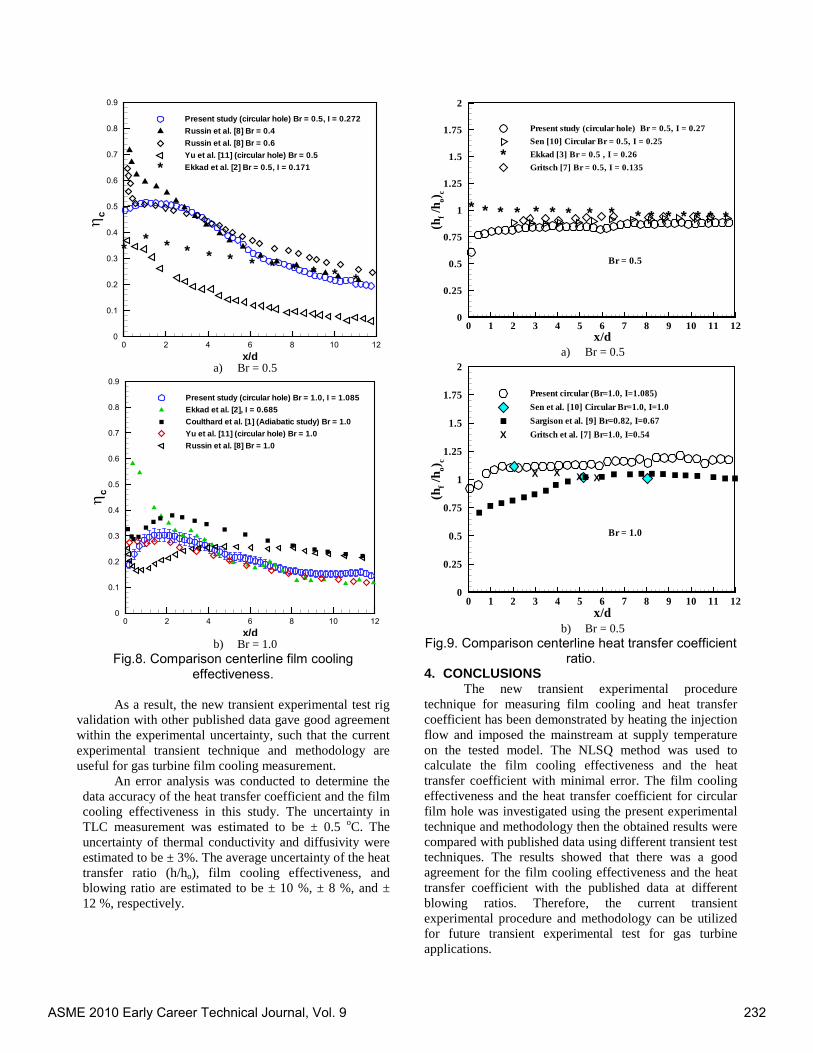
x/d

η c

0 2 4 6 8 10 120

0.1

0.2

0.3

0.4

0.5

0.6

0.7

0.8

0.9

Present study (circular hole) Br = 0.5, I = 0.272Russin et al. [8] Br = 0.4Russin et al. [8] Br = 0.6Yu et al. [11] (circular hole) Br = 0.5Ekkad et al. [2] Br = 0.5, I = 0.171*

a) Br = 0.5

x/d

η c

0 2 4 6 8 10 120

0.1

0.2

0.3

0.4

0.5

0.6

0.7

0.8

0.9

Present study (circular hole) Br = 1.0, I = 1.085Ekkad et al. [2], I = 0.685Coulthard et al. [1] (Adiabatic study) Br = 1.0Yu et al. [11] (circular hole) Br = 1.0Russin et al. [8] Br = 1.0

b) Br = 1.0

Fig.8. Comparison centerline film cooling effectiveness.

As a result, the new transient experimental test rig

validation with other published data gave good agreement within the experimental uncertainty, such that the current experimental transient technique and methodology are useful for gas turbine film cooling measurement.

An error analysis was conducted to determine the data accuracy of the heat transfer coefficient and the film cooling effectiveness in this study. The uncertainty in TLC measurement was estimated to be ± 0.5 oC. The uncertainty of thermal conductivity and diffusivity were estimated to be ± 3%. The average uncertainty of the heat transfer ratio (h/ho), film cooling effectiveness, and blowing ratio are estimated to be ± 10 %, ± 8 %, and ± 12 %, respectively.

* * * * * * * * * * * * * * * *

x/d

(hf/h

o) c

0 1 2 3 4 5 6 7 8 9 10 11 120

0.25

0.5

0.75

1

1.25

1.5

1.75

2

Present study (circular hole) Br = 0.5, I = 0.27Sen [10] Circular Br = 0.5, I = 0.25Ekkad [3] Br = 0.5 , I = 0.26Gritsch [7] Br = 0.5, I = 0.135

*

Br = 0.5

a) Br = 0.5

X X X X

x/d

(hf/h

o)c

0 1 2 3 4 5 6 7 8 9 10 11 120

0.25

0.5

0.75

1

1.25

1.5

1.75

2

Present circular (Br=1.0, I=1.085)Sen et al. [10] Circular Br=1.0, I=1.0Sargison et al. [9] Br=0.82, I=0.67Gritsch et al. [7] Br=1.0, I=0.54X

Br = 1.0

b) Br = 0.5

Fig.9. Comparison centerline heat transfer coefficient ratio.

4. CONCLUSIONS The new transient experimental procedure

technique for measuring film cooling and heat transfer coefficient has been demonstrated by heating the injection flow and imposed the mainstream at supply temperature on the tested model. The NLSQ method was used to calculate the film cooling effectiveness and the heat transfer coefficient with minimal error. The film cooling effectiveness and the heat transfer coefficient for circular film hole was investigated using the present experimental technique and methodology then the obtained results were compared with published data using different transient test techniques. The results showed that there was a good agreement for the film cooling effectiveness and the heat transfer coefficient with the published data at different blowing ratios. Therefore, the current transient experimental procedure and methodology can be utilized for future transient experimental test for gas turbine applications.


ACKNOWLEDGMENTS The author acknowledges Dr. Ibrahim Hassan for

his advice in this work and also acknowledges Pratt and Whitney Canada (PWC) and Concordia University for their support.

REFERENCES 1. Coulthard, Sarah M., Volino, R. J., and Flack, K. A.,

“Effect of unheated starting lengths on film cooling experiments”, Journal of Turbomachinery, vol. 128, no. 3, 2006, pp. 579-588.

2. Ekkad, S. V., Zapata, D., and Han, J. C., “Film effectiveness over a flat surface with air and CO2 injection through compound angle holes using a transient liquid crystal image method”, Journal of Turbomachinery, vol. 119, no. 3, 1997, pp. 587-593.

3. Ekkad, S. V., Zapata, D., Han, J. C., “Heat transfer coefficients over a flat surface with air and CO2 injection through compound angle holes using a transient liquid crystal image method”, American Society of Mechanical Engineers (Paper), 1995, 9pp.

4. Ekkad, S., Shichuan, O., and Rivir, R., “transient infrared thermography method for simultaneous film cooling effectiveness and heat transfer coefficient measurements from a single test”, Journal of Turbomachinery, vol. 126, no. 4, 2004, pp. 597-603.

5. Ekkad, S.V., Han, J.C. and Du, H., “Detailed film cooling measurements on a cylindrical leading edge model: Effect of free-stream turbulence and coolant density”, Journal of Turbomachinery, vol. 120, no. 4, 1998, pp. 799-807.

6. Ghorab, M. G., “Experimental investigation of advanced film cooling schemes for a gas turbine blade”, Ph.D. Thesis, Concordia University, 2009.

7. Gritsch, M., Schulz, A., and Wittig, S., “Adiabatic wall effectiveness measurements of film-cooling holes with expanded exits”, Journal of Turbomachinery, vol. 120, 1998, pp. 549-556.

8. Russin, Rebekah A., Alfred, Daniel, and Wright, Lesley M., “Measurement of detailed heat transfer coefficient and film cooling effectiveness distributions using PSP and TSP”, ASME, Turbo Expo 2009, GT2009- 59975.

9. Sargison, J. E., Guo, S. M., Oldfield, M. L. G., Lock, G. D., and Rawlinson, A. J., “A converging slot-hole film-cooling geometry – part 1: low-speed flat-plate heat transfer and loss”, Journal of Turbomachinery, vol. 124, 2002, pp. 453-460.

10. Sen, Basav, Schmidt, Donald L., and Bogard, David G, “Effects of surface roughness on film cooling”, American Society of Mechanical Engineers, 1996, 7pp.

11. Yu, Y., Yen, C.-H., Shih, T. I.-P., Chyu, M. K., Gogineni, S., “Film cooling effectiveness and heat transfer coefficient distributions around diffusion shaped holes”, Journal of Heat Transfer, vol. 124, n 5, 2002, pp. 820-827.


http://0-www.engineeringvillage.com.mercury.concordia.ca/controller/servlet/Controller?CID=quickSearchCitationFormat&searchWord1=%7bEkkad%2C+Srinath+V.%7d&section1=AU&database=3&yearselect=yearrange&sort=yr�

http://0-www.engineeringvillage.com.mercury.concordia.ca/controller/servlet/Controller?CID=quickSearchCitationFormat&searchWord1=%7bRivir%2C+Richard+B.%7d&section1=AU&database=3&yearselect=yearrange&sort=yr�

http://0-www.engineeringvillage.com.mercury.concordia.ca/controller/servlet/Controller?CID=expertSearchCitationFormat&searchWord1=%7bEkkad%2C+S.V.%7d+WN+AU&database=3&yearselect=yearrange&searchtype=Expert&sort=yr�

http://0-www.engineeringvillage.com.mercury.concordia.ca/controller/servlet/Controller?CID=expertSearchCitationFormat&searchWord1=%7bHan%2C+J.C.%7d+WN+AU&database=3&yearselect=yearrange&searchtype=Expert&sort=yr�

http://0-www.engineeringvillage.com.mercury.concordia.ca/controller/servlet/Controller?CID=expertSearchCitationFormat&searchWord1=%7bDu%2C+H.%7d+WN+AU&database=3&yearselect=yearrange&searchtype=Expert&sort=yr�

http://0-www.engineeringvillage2.org.mercury.concordia.ca/controller/servlet/Controller?CID=quickSearchCitationFormat&searchWord1=%7BSen%2C+Basav%7D&section1=AU&database=3&yearselect=yearrange&sort=yr�

http://0-www.engineeringvillage2.org.mercury.concordia.ca/controller/servlet/Controller?CID=quickSearchCitationFormat&searchWord1=%7BSchmidt%2C+Donald+L.%7D&section1=AU&database=3&yearselect=yearrange&sort=yr�

AUTHOR INDEX

AKHTAR, IMRAN 189

AL ANSARY, HANY 198

ALEXANDER, RYAN C. 158

ALI, MOHAMMED 75

ALMAGABLEH, AHMAD 35

ALUKO, OLANREWANJU 19

ASFAND, FAISAL 112

BANI-YOUNES, AHMAD 96

BEALE, DAVID G. 215

BORGGAARD, JEFF 189

BRANSCOMB, DAVID J. 215, 221

BROUGHTON, Jr., ROYALL M. 215

CERKEZ, IDRIS 221

CHIANG, HSIAO-WEI D. 66

DEMAY, MARK A. 158

MANUSCRIPT REMOVED 49, 57

DOWNS, ROY 41

EMRAN, TAMIR A. 158

FARAH, BASIL I. 173

FUNG, ALAN S. 66

GASTON, N. 178

GHORAB, MOHAMED G. 226

GOLOB, MATTHEW 203

GORDON, ALI P. 181

HASAN, ZEAID F. 96

HEMPOWICZ, MICHAEL 178

HICKMAN, GREGORY J. 88

HSIAO, KUANG-TING 88, 173, 178

ILIESCU, TRAIAN 189

JEFFERSON, GAIL D. 173, 178

JETER, SHELDON 198, 203

JIANG, TAO 9

KRAFT, STEVEN M. 181

KULATHU, SANDEEP 1

LITTLEFIELD, DAVID L. 1

MANTENA, P. RAJU 35

MARINACCI, FRANK 181

MATTHEWS, JENNA 124

McDONALD, DALE 165

McFALL, KEVIN S. 27

MELSERT, RYAN 198

MOORE, BRIAN S. 19

MULLEN, CHRISTOPHER L. 105

MUNN, BRIAN S. 208

NAGARSHETH, HEMANT 138

NANDIKOLLA, VIDYA K. 118, 124

PANDEY, SUNIL 80

PHARKUTE, SUHAS S. 118, 124

PRESNELL, MICHAEL B. 153

RAJENDRAN, ARUNACHALAM M. 153

RAO, R. V. 146

RENCIS, JOSEPH J. 41

SADOWSKI, DENNIS 203

SAVSANI, POONAM V. 138

SAVSANI, VIMAL J. 146

SCHOEN, MARCO P. 124

SCRIVENER, DAKOTA 41

MANUSCRIPT REMOVED. 49, 57

STALLINGS, CHRIS T. 158

TADEPALLI, TEZESWI P. 105

TERDALKAR, SACHIN S. 41

TURK, MATTHEW 198


AUTHOR INDEX (continued)

VAKHARIA, D. P. 146

MANUSCRIPT REMOVED 49, 57

WANG, ZHU 189

WATTAL, REETA 80

ZABIHIAN, FARSHID 66

ZUNDEL, BRADLEY L. 130

ISBN 978-1-4507-9222-6


HEAT TRANSFER FROM FLAT SURFACES TO MOVING … · HEAT TRANSFER FROM FLAT SURFACES TO MOVING SAND...

Documents

Transcript of HEAT TRANSFER FROM FLAT SURFACES TO MOVING … · HEAT TRANSFER FROM FLAT SURFACES TO MOVING SAND...