HEAT TRANSFER AND PRESSURE DROP CHARACTERISTICS OF … · pressure drop across the test section,...
145
HEAT TRANSFER AND PRESSURE DROP CHARACTERISTICS OF SMOOTH TUBES AT A CONSTANT HEAT FLUX IN THE TRANSITIONAL FLOW REGIME by Melissa Hallquist Submitted in partial fulfilment of the requirements for the degree of MASTER OF ENGINEERING Mechanical Engineering in the Faculty of Engineering, Built Environment and Information Technology University of Pretoria December 2011 Supervisor: Prof JP Meyer
Transcript of HEAT TRANSFER AND PRESSURE DROP CHARACTERISTICS OF … · pressure drop across the test section,...

HEAT TRANSFER AND PRESSURE DROP
CHARACTERISTICS OF SMOOTH TUBES AT
A CONSTANT HEAT FLUX IN THE
TRANSITIONAL FLOW REGIME
by
Melissa Hallquist
Submitted in partial fulfilment of the requirements for the degree of
MASTER OF ENGINEERING
Mechanical Engineering in the Faculty of Engineering, Built Environment
and Information Technology
University of Pretoria
December 2011
Supervisor: Prof JP Meyer


iii
ABSTRACT
HEAT TRANSFER AND PRESSURE DROP CHARACTERISTICS OF SMOOTH TUBES AT A CONSTANT HEAT FLUX IN THE TRANSITIONAL FLOW REGIME
Author: M Hallquist
Supervisor: Prof JP Meyer
Department: Mechanical and Aeronautical Engineering
Degree: Master of Engineering (Mechanical Engineering)
Due to constraints and changes in operating conditions, heat exchangers are often forced to operate under conditions of transitional flow. However, the heat transfer and flow behaviour in this regime is relatively unknown. By describing the transitional characteristics it would be possible to design heat exchangers to operate under these conditions and improve the efficiency of the system.
The purpose of this study was to experimentally measure the heat transfer and pressure drop characteristics of smooth tubes at a constant heat flux in the transitional flow regime. The measurements were used to describe the flow behaviour of this regime and attempt to develop a correlation that can be used in the design of a heat exchanger.
An experimental set-up was developed, consisting of an overall set-up, a removable test section as well as a controller, which ensured a uniform heat flux boundary. The test section allowed for the measurement of the temperature along the length of the test section, the pressure drop across the test section, the heat flux input and the flow rate. The measurements were used to determine the heat transfer coefficients and friction factor of the system.
Three test sections were developed with outer diameters of 6, 8 and 10 mm in order to investigate the influence of heat exchanger size. Each test section was subject to four different heat flux cases of approximately 1 500, 3 000, 4 500 and 6 000 W/m2. The experiments covered a Reynolds number range of 450 to 10 300, a Prandtl number range of 4 to 7, a Nusselt number range of 2.3 to 67, and a Grashoff number range of 60 to 23 000.
Good comparison was found between the measurements of this experiment and currently available literature. The experiments showed a smooth transition from laminar to turbulent flow with the onset of transition dependent on the heat flux of the system and with further data capturing, a correlation can be found to describe the Nusselt number in the transitional flow regime.
Keywords: smooth tube, constant heat flux, transition, heat transfer coefficients


v
ACKNOWLEDGEMENTS
This study could not have been completed without the help and encouragement of several individuals:
• First and foremost I would like to thank my study leader for the continued support and encouragement throughout this study;
• Mr D Gouws for setting up of the overall test section necessary to conduct these experiments;
• Mr C Coetzee for the design and construction of the current controller required for the boundary condition considered;
• My fellow students for the company in the laboratory;
• My family for their words of encouragement and support.
The following organisations are thanked for their financial support:
• University of Pretoria;
• Technology and Human Resources for Industry Programme (THRIP) – AL631
• Tertiary Education Support Programme (TESP) from Eskom
• National Research Foundation
• SANERI/Stellenbosch University Solar Hub
• The EEDSM Hub of the University of Pretoria

vii
TABLE OF CONTENTS
Abstract ..................................................................................................................................... iii
Acknowledgements .................................................................................................................... v
Table of Contents ..................................................................................................................... vii
List of Appendices .................................................................................................................... ix
List of Figures ........................................................................................................................... xi
List of Tables ............................................................................................................................ xv
List of Symbols ...................................................................................................................... xvii
1. Introduction ......................................................................................................................... 1
1.1 Background .................................................................................................................1
1.2 Objectives ....................................................................................................................3
2. Literature Study ................................................................................................................... 5
2.1 Introduction .................................................................................................................5
2.2 Fundamentals of Fluid Flow .......................................................................................5
2.2.1 Background ......................................................................................................5
2.2.2 Factors Influencing Laminar and Turbulent Flow ..........................................5
2.2.3 Friction Factors and Pressure Drop ...............................................................6
2.3 Fundamentals of Heat Transfer ..................................................................................8
2.3.1 Thermal Boundary Conditions ........................................................................8
2.3.2 Forms of Heat Transfer .................................................................................. 10
2.3.3 Heat Transfer Parameters .............................................................................. 12
2.4 Nusselt Number Correlations ................................................................................... 13
2.4.1 Laminar Flow .................................................................................................. 13
2.4.2 Turbulent Flow ............................................................................................... 15
2.4.3 Transitional Flow............................................................................................ 17
2.5 Entrance Region and Entrance Effects .................................................................... 24
2.6 Conclusions ............................................................................................................... 26
3. Experimental Procedure ................................................................................................... 27
3.1 Introduction ............................................................................................................... 27
3.2 Experimental Set-up .................................................................................................. 27
3.2.1 Overall Set-up ................................................................................................. 27
3.2.2 Test Section .................................................................................................... 28
3.2.3 Control System .............................................................................................. 30
3.3 Experimental Procedure ........................................................................................... 32
3.3.1 Measurement Procedure ............................................................................... 32
3.3.2 Data Reduction ............................................................................................... 32
3.4 Uncertainties.............................................................................................................. 38

viii
3.4.1 Instruments .................................................................................................... 38
3.4.2 Fluid Properties .............................................................................................. 41
3.4.3 Calculated Parameters .................................................................................. 41
3.5 System Validation ..................................................................................................... 45
3.5.1 Adiabatic friction factors ............................................................................... 46
3.5.2 Diabatic friction factors ................................................................................. 47
3.5.3 Average Nusselt Number ............................................................................... 48
3.5.4 Local Nusselt Number ................................................................................... 50
3.5.5 j Factor ............................................................................................................ 52
3.5.6 Summary ........................................................................................................ 53
4. Results ............................................................................................................................... 55
4.1 Introduction ............................................................................................................... 55
4.2 Diabatic Friction Factors........................................................................................... 55
4.3 Heat Transfer ............................................................................................................. 60
4.3.1 Local Nusselt Number ................................................................................... 63
4.3.2 Average Nusselt Number ............................................................................... 69
4.3.3 Fully Developed Nusselt Number ................................................................. 71
4.3.4 The j Factor..................................................................................................... 72
4.3.5 Conclusions ................................................................................................... 74
5. Analysis of Results ........................................................................................................... 77
5.1 Introduction ............................................................................................................... 77
5.2 The j Factor ................................................................................................................ 77
5.3 Grashoff Number ....................................................................................................... 81
5.4 Summary .................................................................................................................... 91
6. Summary, Conclusions and Recommendations ............................................................. 93
6.1 Summary .................................................................................................................... 93
6.2 Conclusions ............................................................................................................... 93
6.3 Recommendations for Future Work ......................................................................... 94
7. References ......................................................................................................................... 97
Appendix A ............................................................................................................................. 101
Appendix B ............................................................................................................................. 109

ix
LIST OF APPENDICES
Appendix A: Uncertainties
A.1 Current Measurement
A.2 6mm Tube Results
A.2.1 Friction Factor
A.2.2 Local Nusselt Number
A.2.3 Average Nusselt Number
A.3 8mm Tube Results
A.3.1 Friction Factor
A.3.2 Local Nusselt Number
A.3.3 Average Nusselt Number
Appendix B: Data Reduction Spreadsheets
B.1 Tube Characteristics
B.1.1 6 mm Tube
B.1.2 8 mm Tube
B.1.3 10 mm Tube
B.2 Average Results
B.3 Local Results
B.4 Validated Results


xi
LIST OF FIGURES
Figure 2-1: Change in fluid and wall temperatures along the length of a heat exchanger with a constant heat flux boundary: (a) the case of heating the fluid, (b) the case of cooling the fluid ............................................................................................8
Figure 2-2: Variation of fluid and wall temperatures along the length of the heat exchanger with a constant wall temperature boundary: (a) the case of heating fluid in the inner tube, (b) the case of cooling the fluid ................................................................9
Figure 2-3: Fluid and wall temperature distributions for neither boundary condition: (a) the case of heating the fluid on the inner tube, (b) the case of cooling ............................9
Figure 2-4: Mixing of internal forced convection due to natural convection currents ................... 10
Figure 2-5: Flow regimes for forced, free and mixed convection for flow through horizontal tubes (Metais & Eckert 1964) .................................................................................. 11
Figure 2-6: Comparison of laminar correlations for a constant heat flux (3 000 W/m2) ............... 14
Figure 2-7: Nusselt number correlations for laminar to turbulent flow (3 000 W/m2) ................... 19
Figure 2-8: The development of the velocity profile in a circular tube (Cengel 2006) .................. 24
Figure 2-9: The development of the thermal boundary layer in a circular tube (Cengel 2006) ...................................................................................................................... 25
Figure 2-10: Simultaneous development of thermal and velocity profile ....................................... 25
Figure 2-11: Fully developed velocity profile prior to heating ........................................................ 26
Figure 3-1: Process Diagram for Test Set-up ............................................................................. 27
Figure 3-2: Test section ............................................................................................................. 28
Figure 3-3: Percentage heat lost through the insulation for the 6 mm tube at a heat flux of 5 346 W/m2 ............................................................................................................. 29
Figure 3-4: Flow diagram for the operation of the control system ............................................... 31
Figure 3-5: Calculation of local fluid temperature ....................................................................... 34
Figure 3-6: Illustration of expected temperature distribution ....................................................... 35
Figure 3-7: Calibration curve for channel 105 in the 6 mm tube test case .................................. 39
Figure 3-8: Calibration curve for the pressure transducer .......................................................... 40
Figure 3-9: Expected uncertainties of the average Nusselt number in the 10 mm tube at different heat fluxes ................................................................................................. 43
Figure 3-10: Uncertainties of Local Nusselt numbers at various heat fluxes ................................ 44
Figure 3-11: Expected uncertainties of friction factor in the 10 mm tube at different heat fluxes ...................................................................................................................... 45
Figure 3-12: Adiabatic friction factor for the 6 mm tube ................................................................ 46
Figure 3-13: Diabatic friction factor for the 6 mm tube at a heat flux of 2 832 W/m2 ..................... 48
Figure 3-14: Nusselt number for the 6 mm tube at a heat flux of 2 832 W/m2 .............................. 49
Figure 3-15: Laminar Nusselt number results for the 6 mm tube at a heat flux of 2 832 W/m2 ..... 49
Figure 3-16: Local Nusselt number for the 6 mm test tube for a Reynolds number of 1 540 at a heat flux of 2 832 W/m2 .................................................................................... 50
Figure 3-17: Temperature distribution for the 6 mm tube for a Reynolds number of 1 540 at a heat flux of 2 832 W/m2 ........................................................................................ 51
Figure 3-18: Local Nusselt number for the 6 mm tube for a Reynolds number of 1 540 at a heat flux of 2 832 W/m2after correcting the wall temperature .................................. 51

xii
Figure 3-19: Comparison to the results of Ghajar and Tam (1994) for the 6 mm tube at 2 832 W/m2K .......................................................................................................... 52
Figure 4-1: Average diabatic friction factors for different heat fluxes for the 10 mm tube: (a) full Reynolds number range, (b) transition region ................................................... 56
Figure 4-2: Average friction factors over the test section measured for all heating cases of the 6 mm tube: (a) full Reynolds number range, (b) transition region ................... 57
Figure 4-3: Average friction factor over the 8 mm test section: (a) full Reynolds number range, (b) transition region ...................................................................................... 58
Figure 4-4: Comparison of friction factor across the different tube sizes .................................... 59
Figure 4-5: Raleigh number results for all the test cases ........................................................... 61
Figure 4-6: Temperature profile for the 10 mm test section at a heat flux of 6 505 W/m2 ........... 62
Figure 4-7: Local heat transfer ratio for the 10 mm test case at a heat flux of 6 505 W/m2 ......... 62
Figure 4-8: Local Nusselt numbers for the 6 mm test case at an average Reynolds number of approximately 1 845 ........................................................................................... 64
Figure 4-9: Local Nusselt number at Reynolds number of 1 869 for the 8 mm test section ........ 65
Figure 4-10: Local Nusselt number for the 10 mm test case at an average Reynolds number of approximately 1 843 ........................................................................................... 65
Figure 4-11: Turbulent results for the local Nusselt number for the 6 mm test case at a Reynolds number of 5 355 ...................................................................................... 66
Figure 4-12: Turbulent results for the local Nusselt number for the 10 mm test case at a Reynolds number of 5 376 ...................................................................................... 67
Figure 4-13: Transitional local Nusselt numbers for the 10 mm test case at a Reynolds number of 2 467 ..................................................................................................... 68
Figure 4-14: Average Nusselt number for the 10 mm tube........................................................... 69
Figure 4-15: Average Nusselt number for the 6 mm tube ............................................................ 70
Figure 4-16: Average Nusselt number for the 8 mm tube ............................................................ 71
Figure 4-17: Fully developed Nusselt number for the 10 mm tube ............................................... 72
Figure 4-18: The j Factor for the 10 mm tube ............................................................................... 73
Figure 4-19: The j Factor for the 6 mm tube................................................................................. 73
Figure 4-20: Stanton number for the 8 mm tube .......................................................................... 74
Figure 5-1: Colburn j factor and friction factor for the 10 mm tube plotted as a function of the Reynolds number .............................................................................................. 77
Figure 5-2: Corrected Colburn j factor and friction factor for the 10 mm tube plotted as a function of the Reynolds number ............................................................................ 78
Figure 5-3: Corrected Colburn j factor (4Pr2/3) and friction factor for the 10 mm tube plotted as a function of the Reynolds number ..................................................................... 79
Figure 5-4: Corrected Colburn j factor (4.7Pr2/3) and friction factor for the 10 mm tube plotted as a function of the Reynolds number ......................................................... 79
Figure 5-5: Corrected Colburn j factor (4.7Pr2/3) and friction factor for the 6 mm tube plotted as a function of the Reynolds number ..................................................................... 80
Figure 5-6: Corrected Colburn j factor (4.7Pr2/3) and friction factor for the 8 mm tube plotted as a function of the Reynolds number ..................................................................... 81
Figure 5-7: Grashoff number for the 10 mm results given as a function of the Reynolds number, viscosity ratio and Nusselt number ............................................................ 82
Figure 5-8: Grashoff number for the 8 mm results given as a function of the Reynolds number, viscosity ratio and Nusselt number ............................................................ 83

xiii
Figure 5-9: Grashoff number for the 6 mm results given as a function of the Reynolds number, viscosity ratio and Nusselt number ............................................................ 83
Figure 5-10: Curve fit for the 8 mm transitional flow data ............................................................. 84
Figure 5-11: Curve fit for the 6 mm transitional flow data ............................................................. 85
Figure 5-12: Curve fit for the 10 mm transitional flow data ........................................................... 85
Figure 5-13: Curve fit for all transitional flow data ........................................................................ 86
Figure 5-14: Curve fit for the different test cases at the highest heat flux condition ...................... 87
Figure 5-15: A correlation for the results of the highest heat flux condition .................................. 87
Figure 5-16: Evaluation of the correlation for the highest heat flux case ...................................... 88
Figure 5-17: A correlation for an average heat flux of 4 450 W/m2 ............................................... 89
Figure 5-18: A correlation for an average heat flux of 3 080 W/m2 ............................................... 90


xv
LIST OF TABLES
Table 2-1: Constants and limitations of equation 5 (Ghajar & Madon 1992) .................................. 7
Table 2-3: Constants and limitations for equation 27 (Ghajar & Tam 1994) ................................. 18
Table 2-4: Summary of Nusselt number correlations ................................................................... 21
Table 3-1: Diaphragm sizes used ................................................................................................ 39
Table 3-2: Expected uncertainty for each diaphragm .................................................................. 40
Table 3-3: Fluid property uncertainties (Popiel and Wojtkowiak, 1998)........................................ 41
Table 3-4: Overall uncertainties for all of the test cases combined .............................................. 42


xvii
LIST OF SYMBOLS
Symbol Description Units Variations
A Area m2 As Surface area
Ac Cross-sectional area
b Bias -
Cf Friction coefficient -
Cp Specific heat J/kg.K
d Diameter m di Inner diameter
do Outer diameter
f Friction factor
g Gravitational force m2/s
Gr Grashoff number -
Gz Graetz number -
h Heat transfer
coefficient
W/m2.K hfd Fully developed heat transfer coefficient
h(x) Local heat transfer coefficient
h Average heat transfer coefficient
i Current A
k Thermal conductivity W/m.K k(x) Local thermal conductivity
k Average thermal conductivity
L Length m Lh Hydrodynamic entrance length
Lt Thermal entrance length
Lfd Fully developed tube length
.
m Mass flow kg/s
Nu Nusselt number - Nul Laminar Nusselt number
Nut Turbulent Nusselt number
Nu(x) Local Nusselt number
Nufd Fully developed Nusselt number
Nu Average Nusselt number
Nul,c Laminar Nusselt number at Re = 2100
Nu0
Asymptotic Nusselt number (Churchill
1977)

xviii
P Pressure Pa
p Precision -
Pr Prandtl number -
.
Q Heat transfer W elec
.
Q Electric power
.
Q Heat transfer
cond
.
Q Conduction heat transfer
conv
.
Q Convection heat transfer
q Heat flux W/m2
R Resistance Ω,W/K R Electrical resistance
R0 Reference electrical resistance
Rthermal Thermal resistance
Ra Raleigh number -
Re Reynolds number -
St Stanton number -
T Temperature °C Ts Surface temperature
sT Average surface temperature
Tsi Inner-surface temperature
Tso Outer-surface temperature
Tf Fluid temperature
Tf,i Inlet bulk fluid temperature
Tfo Outlet bulk fluid temperature
Tb Bulk fluid temperature
v Velocity m/s vx Local velocity
v Average velocity
V Voltage V
x Position m
ρ Density kg/m3
µ Dynamic viscosity kg/m.s µb Bulk fluid dynamic viscosity
µw Dynamic viscosity at the wall
temperature
β Volume expansivity 1/K

xix
σ Resistivity Ω.m
ν Kinematic viscosity m2/s
τw Wall shear stress N/m2
δ Uncertainty -
∆ Difference/change -

Analysis of Theoretical Heat Transfer Coefficients for Laminar to Turbulent Flow in Smooth Tubes
Melissa Hallquist
Chapte
r: In
troduction
1
1. INTRODUCTION
1.1 BACKGROUND
One of the more important applications of heat transfer is found in the energy industry where various processes rely on the heating or cooling of fluid inside tubes. The study and design of these systems require extensive knowledge of the heat transfer coefficients between the wall of the tube and the fluid flowing inside it. A fundamental understanding of heat transfer coefficients would therefore assist in improving the efficiency of systems like these.
Heat transfer can take place under three different thermal boundary conditions. Firstly, a uniform heat flux boundary condition, which is generally applied to a practical situation of electric resistance heating and nuclear applications. Secondly, a uniform wall temperature boundary, which is approached when the outer-tube surface of a heat exchanger is heated by an isothermally condensing fluid or likewise cooled by an isothermally boiling fluid. The third boundary condition is achieved when neither a uniform heat flux or uniform wall temperature boundary is applied, which is the case in certain tube-in-tube heat exchangers.
Convective heat transfer is governed by fluid flow and therefore the flow regimes (laminar, transitional and turbulent flow) must be considered in addition to the different thermal boundaries. Osbourne Reynolds successfully identified the existence of transitional flow in the late 1800s and in the absence of free convection effects, the flow regime is solely dependent on the Reynolds number (Engineering Science Data Unit (ESDU) 1993).
Laminar flow in a round tube exists when the Reynolds number is less than 2 300 (ASHRAE 2009). Fully turbulent flow exists when the Reynolds number is larger than 10 000 and therefore transitional flow (where the fluid motion changes from laminar to turbulence) exists for Reynolds numbers between 2 300 and 10 000. ASHRAE further states that predictions are unreliable in this transitional flow regime. Cengel (2006) mentions that although transitional flow exists for Reynolds numbers between 2 300 and 10 000, it should be kept in mind that in many cases, the flow becomes fully turbulent for a Reynolds number as low as 4 000.
The Nusselt number is described differently for each of these regimes.
For laminar flow, the Nusselt number is documented to be a constant, the value of which depends on the thermal boundary condition. For a uniform heat flux boundary, the Nusselt number is known to be 4.36 and for a uniform wall temperature, the value is 3.66 (Cengel 2006). However, these values are only applicable to flow that is both hydrodynamically and thermodynamically fully developed without secondary flow effects.
In the turbulent regime, the Nusselt number is commonly a function of the Reynolds number and Prandtl number and is no longer a constant value. The most commonly used relationships include those developed by experts such as Petukhov, Polyakov and Strigin (1969), Dittus and Boelter (1930), Sieder and Tate (1936) and Gnielinski (1977). However, these correlations differ quite significantly from one another. When comparing the values calculated from the different relationships, errors of up to 30% can be made. This means that when designing a heating or cooling system, the system can either be underdesigned by as much as 30%, or overdesigned by 30%. The result is either an inefficient system or an expensive one.
It is normally advised to remain outside the transitional flow regime when designing a heat exchanger. This is due to the uncertainty of the regime and the flow instability associated with transitional flow. For this reason, little design information is available with specific reference to Nusselt number associated with this regime. However, size constraints and changes in

University of Pretoria
Department of Mechanical and Aeronautical Engineering
Chapte
r: In
troduction
2
operating conditions often result in heat exchangers operating under these unknown conditions.
A good design of a heat exchanger should consider methods of increasing heat transfer performance while reducing the pressure drop (Shokouhmand & Salimpour 2007). Turbulent flow provides the best heat transfer coefficients with the disadvantage of high pressure drops, whereas the opposite is true for laminar flow. The alternative is to consider transitional flow, which could provide better heat transfer characteristics than laminar flow with lower pressure drops compared with turbulent flow.
With increasing energy prices and a demand for energy saving, the study of heat transfer behaviour in the transitional flow regime is of considerable importance. Despite numerous studies conducted on this flow regime, the underlying physics and the implications of this phenomenon have eluded complete understanding (Olivier & Meyer 2010).
One such study was conducted by Ghajar and Tam (1994). Experiments were carried out which considered a uniform heat flux boundary condition for distilled water and mixtures of distilled water and ethylene glycol. The experiments covered a Reynolds number range of 280 to 49 000, a Prandtl number range of 4 to 158 and a Grashoff number range of 1 000 to 2.5 E 5. The test section considered had an internal diameter of 15.8 mm and was subject to a heat flux of between 4 and 670 kW/m2. The influence of different entrance sections and their influence on transition were investigated.
The purpose of this study was to create a database for forced and mixed convection heat transfer for a wide range of Reynolds, Prandtl and Grashoff numbers. For each of the flow regimes, a correlation was developed for the local Nusselt number. The correlation is subject to a number of restrictions based on tube size, viscosity ratio, Reynolds number, Grashoff number and Prandtl number. A single correlation for transitional flow could not predict all the data and a separate correlation for each inlet configuration had to be determined.
Olivier and Meyer (2010) conducted a study to investigate the behaviour of a heat exchanger in the transitional flow regime with different inlet geometries. Pressure drop and heat transfer readings were taken under diabatic and adiabatic conditions. Experiments were conducted for smooth tubes in a tube-in-tube counterflow heat exchanger for the isothermal cooling of a fluid. Four different inlet profiles were considered with a Reynolds number range of 1 000 to 20 000, Prandtl number range from 4 to 6 and Grashoff number in the order of 105.
The adiabatic results showed that the transition from laminar to turbulence is dependent on the inlet profile of the test section. This dependence was not seen in the diabatic results due to the suppression of the inlet disturbances by secondary flow effects. The onset of transition in each of the test cases was at a Reynolds number of 2 100. The laminar heat transfer coefficients and friction factors were considerably higher than the theoretical predictions, which has also been attributed to secondary flow effects.
The Reynolds analogy gives a direct relationship between the friction factor and heat transfer coefficients. Based on this philosophy, a correlation was determined for the heat transfer coefficients across the entire flow range, which predicts 88% of the heat transfer data (Olivier & Meyer 2010).
These studies have lent weight to the fact that the transitional flow regime can be accurately described. There are, however, gaps that need to be filled by further investigation into the influence of transition. None of the studies determined the influence of different tube diameters. Both studies (Ghajar & Tam 1994; Olivier & Meyer 2010) focused on the influence of the inlet geometry and highlighted the influence of secondary flow. The influence of increasing heat flux on transition has not been discussed and there is a lack of data for low Prandtl numbers especially in the laminar flow regime.

Analysis of Theoretical Heat Transfer Coefficients for Laminar to Turbulent Flow in Smooth Tubes
Melissa Hallquist
Chapte
r: In
troduction
3
1.2 OBJECTIVES
The purpose of this study was to experimentally measure the heat transfer and pressure drop characteristics of smooth tubes at a constant heat flux in the transitional flow regime. An experimental set-up was developed to measure the temperature, heat flux, flow rate and pressure drop of smooth horizontal tubes. The data collected was used to determine Nusselt numbers and friction factors as a function of Reynolds number. The focus is on the transitional flow regime with a single inlet profile. An entrance section ensured that the flow achieved a fully developed velocity profile before heat was applied to the test tube.
The data collected is to be used to describe the unknown characteristics of flow in the transitional flow regime. It is hoped that this study will lead to increased accuracy of heat transfer calculations and ultimately improve the efficiency of heat transfer systems.
This dissertation consists of six chapters. The following chapter (Chapter 2) takes a look at all the relevant literature available on heat transfer in tubes, which is followed by the experimental procedure (Chapter 3). The experimental procedure describes the test set-up and methods used to capture the relevant data used to calculate the Nusselt number and friction factors. The pressure drop and heat transfer results of each test section are systematically discussed. The results (Chapter 0) are compared with current literature and deviations explained. Finally, the results are analysed (Chapter 0) in order to describe the behaviours captured by these experiments. The summary and conclusions and recommendations are given in Chapter 6.


Analysis of Theoretical Heat Transfer Coefficients for Laminar to Turbulent Flow in Smooth Tubes
Melissa Hallquist
Chapte
r: L
itera
ture
Stu
dy
5
2. LITERATURE STUDY
2.1 INTRODUCTION
Any heat exchanger relies on the mechanism of convection to transfer energy from one fluid to another. To fully understand the design of heat exchangers, one must consider aspects of both fluid flow and heat transfer itself. This literature survey therefore first considers the fundamentals of single-phase fluid flow relevant to heat transfer in tubes before discussing specific heat transfer aspects.
2.2 FUNDAMENTALS OF FLUID FLOW
2.2.1 BACKGROUND
Flow of fluid inside tubes has been a topic of extensive research, which started as early as the 1800s when Osbourne Reynolds first introduced the concept of laminar and turbulent flow. He achieved this by injecting dye into the stream of fluid flow in a tube to distinguish between the two flow regimes – a procedure that is still popular today. Based on his work, Reynolds discovered that the flow regime was highly dependent on the ratio of the inertia forces of the fluid to its viscous forces. For tube flow, this relationship is given as follows and is known as the Reynolds number (White 2003):
µ
ρvdRe = (1)
Fluid flow is said to be laminar when the flow is smooth and usually this occurs at low Reynolds numbers. As the velocity is increased beyond a critical point, the fluid flow becomes chaotic or turbulent. The transition between laminar and turbulent flow does not occur suddenly, but rather occurs over a region where the flow fluctuates between laminar and turbulent flow before becoming fully turbulent.
2.2.2 FACTORS INFLUENCING LAMINAR AND TURBULENT FLOW
The transition from laminar to turbulent flow depends on a number of factors such as the surface geometry, surface roughness, flow velocity, surface temperature and the type of fluid (Cengel 2006).
The critical point of transition is dependent on geometry and the widely accepted boundary for fluid flow in smooth pipes is as follows (Engineering Science Data Unit (ESDU) 1993):
Laminar Flow - 2300<Re
Transitional Flow - 30002300 ≤≤ Re
Turbulent Flow - 3000≥Re
However, it has been documented that for certain inlet conditions, transition can be delayed to Reynolds numbers of up to 10 000 as is the case for very smooth tubes with a bellmouth inlet (Cengel 2006).
The following factors influence the flow regime, which also indirectly influences the heat transfer of flow in tubes (Engineering Science Data Unit (ESDU) 2001):
University of Pretoria
Department of Mechanical and Aeronautical Engineering
Chapte
r: L
itera
ture
Stu
dy
6
2.2.2.1 VARIABLE PHYSICAL PROPERTIES
Radial variations of the fluid properties will occur if there is a large difference between the wall temperature and the bulk temperature of the fluid, or in cases operating near the critical point. Variations of viscosity, thermal conductivity, specific heat capacity and density will affect transition.
For liquids far from their critical points, the thermal conductivity, specific heat capacity and density are weak functions of temperature, but the dynamic viscosity varies significantly with temperature.
2.2.2.2 SURFACE ROUGHNESS
Laminar flow is not affected by surface roughness whereas turbulent flow is affected in the form of increased pressure drop accompanied by an increase in the heat transfer coefficient.
There are two forms of surface roughness: natural roughness and artificial roughness. The natural roughness is generally irregular and is formed during the manufacturing procedure or due to imperfections in the material. Artificial roughness is usually formed in a regular pattern to enhance heat transfer.
2.2.2.3 MIXED CONVECTION
Mixed convection is a combination of free and forced convection, where free convection refers to the motion which occurs in a fluid because of buoyancy forces. This mixed convection could have a significant effect on heat transfer in laminar flow in horizontal tubes as a result of changes in the pattern of convection. The effect is generally to enhance heat transfer, but there are a few cases where the heat transfer is diminished. Mixed convection is discussed further in Section 0.
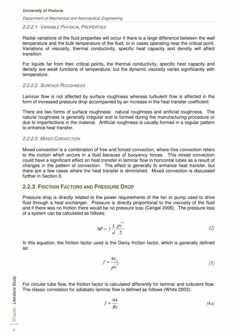
2.2.3 FRICTION FACTORS AND PRESSURE DROP
Pressure drop is directly related to the power requirements of the fan or pump used to drive fluid through a heat exchanger. Pressure is directly proportional to the viscosity of the fluid and if there was no friction there would be no pressure loss (Cengel 2006). The pressure loss of a system can be calculated as follows:
2
2
v
d
LfP
ρ=∆ (2)
In this equation, the friction factor used is the Darcy friction factor, which is generally defined as:
2
8
vf w
ρ
τ= (3)
For circular tube flow, the friction factor is calculated differently for laminar and turbulent flow. The classic correlation for adiabatic laminar flow is defined as follows (White 2003):
Ref
64= (4a)

Analysis of Theoretical Heat Transfer Coefficients for Laminar to Turbulent Flow in Smooth Tubes
Melissa Hallquist
Chapte
r: L
itera
ture
Stu
dy
7
During heating, mixed convection results in secondary flow that influences both the heat transfer of the system and the friction factor (to be discussed in Section 0). To account for this influence, Ghajar and Madon (1992) suggest including a viscosity correction factor to the laminar correlation to account for the increase in friction factors experienced during heating. The resulting correlation is as follows:
m
s
b
Ref
=
µ
µ64 (4b)
where
1708400130651
..GrPr..m −= (4c)
In the same article (Ghajar & Madon 1992), Tam and Ghajar present an equation for the friction factor in the transitional regime defined as follows:
m
s
b
cb
a
Ref
+=
µ
µ14 (5)
This equation is associated with the following constants (a, b and c) and limitations:
Table 2-1: Constants and limitations of equation 5 (Ghajar & Madon 1992)
Inlet m a b c Limitations
Re-entrant 14133046011
..PrGr..m
−−−= 5840 -0.0145 -6.23
2 700 < Re < 5 500
16 < Pr < 35
7 410 < Gr < 158 300
1.13 < µb/ µs < 2.13
Square-edged
151603960131
..PrGr..m
−−−=
4230 -0.16 -6.57
3 500 < Re < 6 900
12 < Pr < 29
6 800 < Gr < 104 500
1.11 < µb/ µs < 1.89
Bellmouth 14133046011
..PrGr..m
−−−= 5340 -0.0990 -6.32
5 900 < Re < 9 600
8 < Pr < 15
11 900 < Gr < 353 000
1.05 < µb/ µs < 1.47
For turbulent flow, the adiabatic friction factor for smooth tubes is described by the Blasius equation as follows:
25031640
.Re.f
−= (6a)

University of Pretoria
Department of Mechanical and Aeronautical Engineering
Chapte
r: L
itera
ture
Stu
dy
8
Allen and Eckert (1964) include a correction factor to the Blasius’ equation to account for viscosity effects during heating in turbulent flow as follows:
250
25031640
.
s
b.Re.f
−
−
=
µ
µ (6b)
The correlation was developed by taking measurements of hydrodynamically fully developed turbulent flow of water entering a uniformly heated smooth tube.
2.3 FUNDAMENTALS OF HEAT TRANSFER
2.3.1 THERMAL BOUNDARY CONDITIONS
There are three different conditions under which heat is transferred in a heat exchanger and each condition has to be treated differently (Engineering Science Data Unit (ESDU) 2001). The influence of the thermal boundary condition is especially significant in laminar flow.
2.3.1.1 UNIFORM HEAT FLUX BOUNDARY
A uniform heat flux (UHF) boundary condition is typical of a tube surrounded by heating tape or an electrical current, or a tube-in-tube heat exchanger where the external heat transfer coefficient is low (Mohammed & Yasin 2007). This results in a wall temperature that tends to decrease along the length of the tube, while the fluid temperature increases (depending on the specific application). As shown in Figure 2-1, the temperature gradients are equal, resulting in a uniform heat flux.
Figure 2-1: Change in fluid and wall temperatures along the length of a heat exchanger with a constant heat flux boundary: (a) the case of heating the fluid, (b) the case of cooling the fluid
2.3.1.2 UNIFORM WALL TEMPERATURE BOUNDARY
The inner tube of the heat exchanger could also be subject to a uniform wall temperature (UWT). This condition can be closely approached when the outside tube surface is heated by an isothermally condensing fluid, or cooled by an isothermally boiling fluid. This condition can also be obtained in counterflow heat exchangers where the heat transfer coefficient and the flowing heat capacity for the external flow are approximately equal to, or much larger than the corresponding values for the flow through the inner tube.

Analysis of Theoretical Heat Transfer Coefficients for Laminar to Turbulent Flow in Smooth Tubes
Melissa Hallquist
Chapte
r: L
itera
ture
Stu
dy
9
There are two cases in which this situation can be implemented: in boilers used for power generation as well as in chillers used for evaporation. The temperature of the fluid can either increase or decrease depending on the specific application shown in Figure 2-2, where Figure 2-2(a) is typical of heating in power generation and Figure 2-2(b) cooling of water in a chiller.
Temperature [°C]
Temperature [°C]
Figure 2-2: Variation of fluid and wall temperatures along the length of the heat exchanger with a constant wall temperature boundary: (a) the case of heating fluid in the inner tube, (b) the case of
cooling the fluid
2.3.1.3 NEITHER BOUNDARY
Finally, the tube wall could have neither of the above boundary conditions, applicable to certain counterflow heat exchangers.
Figure 2-3: Fluid and wall temperature distributions for neither boundary condition: (a) the case of heating the fluid on the inner tube, (b) the case of cooling

University of Pretoria
Department of Mechanical and Aeronautical Engineering
Chapte
r: L
itera
ture
Stu
dy
10
2.3.2 FORMS OF HEAT TRANSFER
There are normally two forms of heat transfer and convection (radiation is not considered in this study)
Conduction is the transfer of energy from particles of higher energy to adjacent particles with less energy as a result of the interaction betweeFourier’s law of heat conduction, the rate of heat conduction through a plane layer is proportional to the temperature difference across the layer and the surface area, but inverselproportional to the thickness of the layer
Convection on the other hand adjacent liquid that is in motion efficient and therefore the resulting convective heat transfer coefficients can be very large (Mills 1992). The faster the fluid motion, the higher the heat transfer. The rate of heat transfer is proportional to the temperature difference and is expressed by Newton’s law of cooling as:
In the case of fluid being pumped through a tube, the heat transfer is said to be forced convection. However, the presence of a temperaturerise to natural convection currents accompanied by natural convection.
Natural convection either enhances or inhibits heat transfer dependent on the relative directions of the buoyancy-induced and forced convection motions. In vertical tubes, buoyancy forces either directly oppose or assist forced convection.
In horizontal tubes, buoyancy forces aids in mixing of the fluid (secondary flow) and therefore enhances heat transfer2006). In the case of internal forced convection in by counter-rotating vortices (Figure
Figure 2-4: Mixing of internal forced convection due to natural convection currents
These counter-rotating vortices are superimposed on the stream flowthe pressure drop and the heat transfer. Secondary flow also reduces the thermal entrance length and induces early transition to turbulent flow flow is dependent on Reynolds number, Prandtl number, configurations, thermal boundary conditions and entrance length.
Department of Mechanical and Aeronautical Engineering
RANSFER
two forms of heat transfer in the flow of fluid through a tube(radiation is not considered in this study).
Conduction is the transfer of energy from particles of higher energy to adjacent particles with less energy as a result of the interaction between the particles (Cengel 2006)Fourier’s law of heat conduction, the rate of heat conduction through a plane layer is proportional to the temperature difference across the layer and the surface area, but inverselproportional to the thickness of the layer as follows:
dx
dTkAQ ccond
.
−=
on the other hand is the transfer of energy between a solid surface and the adjacent liquid that is in motion (Cengel 2006). The transport of heat by flowing liquid is very efficient and therefore the resulting convective heat transfer coefficients can be very large
. The faster the fluid motion, the higher the heat transfer. The rate of heat transfer is proportional to the temperature difference and is expressed by Newton’s law of
ThAQ sconv
.
∆=
In the case of fluid being pumped through a tube, the heat transfer is said to be forced he presence of a temperature gradient in a fluid in a gravity field gives
rise to natural convection currents (Cengel 2006). Forced convection is therefore always accompanied by natural convection.
r enhances or inhibits heat transfer dependent on the relative induced and forced convection motions. In vertical tubes,
buoyancy forces either directly oppose or assist forced convection.
In horizontal tubes, buoyancy forces are perpendicular to the forced convection flow, which aids in mixing of the fluid (secondary flow) and therefore enhances heat transfer
ernal forced convection in tube flow, secondary flow isFigure 2-4).
Mixing of internal forced convection due to natural convection currents
ing vortices are superimposed on the stream flow, which increases both the pressure drop and the heat transfer. Secondary flow also reduces the thermal entrance length and induces early transition to turbulent flow (Mohammed & Yasin 2007)
on Reynolds number, Prandtl number, Grashoffconfigurations, thermal boundary conditions and entrance length.
in the flow of fluid through a tube: conduction
Conduction is the transfer of energy from particles of higher energy to adjacent particles with (Cengel 2006). According to
Fourier’s law of heat conduction, the rate of heat conduction through a plane layer is proportional to the temperature difference across the layer and the surface area, but inversely
(7)
is the transfer of energy between a solid surface and the e transport of heat by flowing liquid is very
efficient and therefore the resulting convective heat transfer coefficients can be very large . The faster the fluid motion, the higher the heat transfer. The rate of convection
heat transfer is proportional to the temperature difference and is expressed by Newton’s law of
(8)
In the case of fluid being pumped through a tube, the heat transfer is said to be forced gradient in a fluid in a gravity field gives
. Forced convection is therefore always
r enhances or inhibits heat transfer dependent on the relative induced and forced convection motions. In vertical tubes,
are perpendicular to the forced convection flow, which aids in mixing of the fluid (secondary flow) and therefore enhances heat transfer (Cengel
flow, secondary flow is characterised
Mixing of internal forced convection due to natural convection currents
which increases both the pressure drop and the heat transfer. Secondary flow also reduces the thermal entrance
in 2007). Secondary Grashoff number, inlet
Analysis of Theoretical Heat Transfer Coefficients for Laminar to Turbulent Flow in Smooth Tubes
Melissa Hallquist
Chapte
r: L
itera
ture
Stu
dy
11
For cases of UHF, a wall to fluid temperature differential exists throughout the length of the heat exchanger, therefore secondary flow exists throughout the tube length. For a UWT boundary, the secondary flow develops to a maximum intensity before reducing to zero as the wall to fluid temperature differential diminishes.
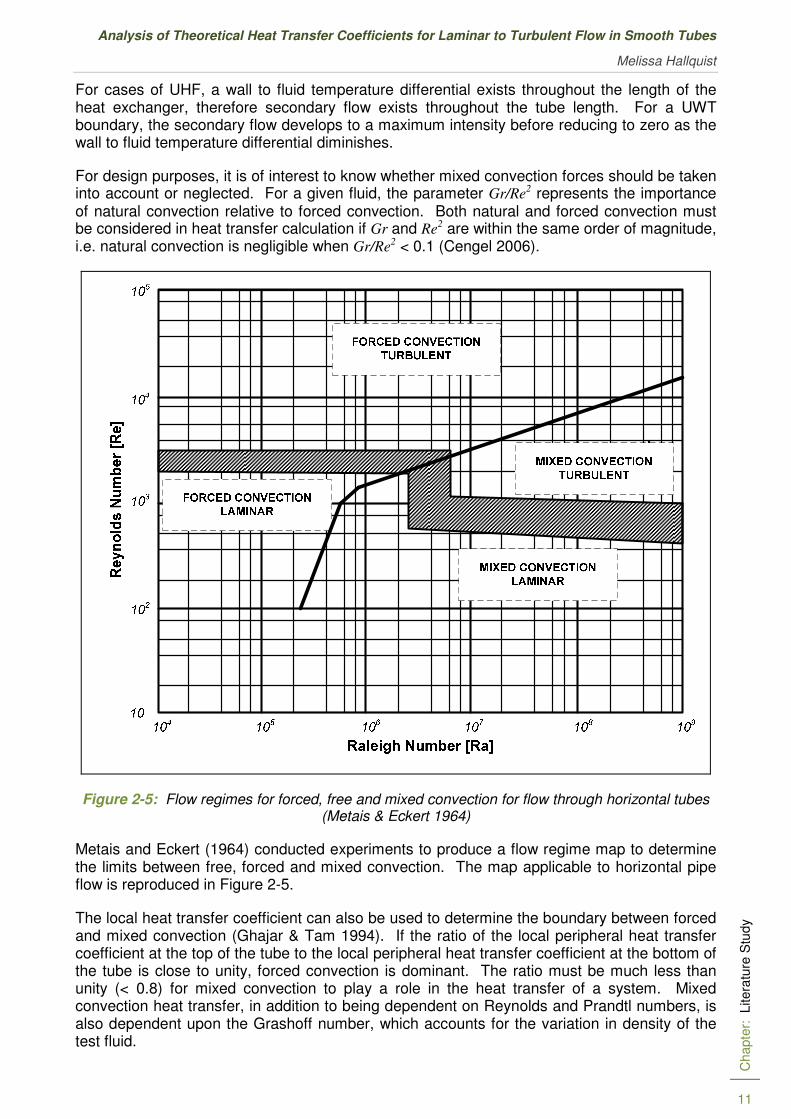
For design purposes, it is of interest to know whether mixed convection forces should be taken into account or neglected. For a given fluid, the parameter Gr/Re2 represents the importance of natural convection relative to forced convection. Both natural and forced convection must be considered in heat transfer calculation if Gr and Re2 are within the same order of magnitude, i.e. natural convection is negligible when Gr/Re2 < 0.1 (Cengel 2006).
Figure 2-5: Flow regimes for forced, free and mixed convection for flow through horizontal tubes (Metais & Eckert 1964)
Metais and Eckert (1964) conducted experiments to produce a flow regime map to determine the limits between free, forced and mixed convection. The map applicable to horizontal pipe flow is reproduced in Figure 2-5.
The local heat transfer coefficient can also be used to determine the boundary between forced and mixed convection (Ghajar & Tam 1994). If the ratio of the local peripheral heat transfer coefficient at the top of the tube to the local peripheral heat transfer coefficient at the bottom of the tube is close to unity, forced convection is dominant. The ratio must be much less than unity (< 0.8) for mixed convection to play a role in the heat transfer of a system. Mixed convection heat transfer, in addition to being dependent on Reynolds and Prandtl numbers, is also dependent upon the Grashoff number, which accounts for the variation in density of the test fluid.
University of Pretoria
Department of Mechanical and Aeronautical Engineering
Chapte
r: L
itera
ture
Stu
dy
12
2.3.3 HEAT TRANSFER PARAMETERS
Heat transfer characteristics are often determined on an experimental basis and in order to aid experiments, important parameters are often expressed in non-dimensional form. Some of the important parameters are given in this section.
The Prandtl number is a dimensionless number named after Ludwig Prandtl who introduced the concept of the boundary layer in 1904. The Prandtl number describes the relative thickness of the velocity and the thermal boundary layers (Cengel 2006) as follows:
k
CPr
pµ= (9)
The Prandtl number relates the temperature distribution to the velocity distribution. When the Prandtl number is small, the temperature gradient near a surface is less steep than the velocity gradient. Conversely, for fluids where the Prandtl number is larger than one, the temperature gradient is steeper than the velocity gradient. At given Reynolds numbers, fluids with larger Prandtl numbers have larger Nusselt numbers (Kreith & Bohn 2001).
In 1885, Graetz originally formulated the solution of a UWT problem for laminar tube flow (Lienhard & Lienhard 2008). The problem was then solved by Sellers, Tribus and Klein in 1965. The solution includes an arrangement of dimensionless pi groups and has been called the Graetz number:
x
dPrReGz = (10)
The Grashoff number is a dimensionless parameter that governs the flow regime in natural convection (Cengel 2006). It represents the ratio of buoyancy forces to viscous forces acting on the fluid and is given by the following equation:
( )2
3
ν
β dTTgGr bs −
= (11)
The Rayleigh number was named after Lord Rayleigh in 1915 (Lienhard & Lienhard 2008). It is associated with buoyancy driven or mixed convection flow. The definition of the Raleigh number is as follows:
PrGrRa = (12)
It is of vital importance to know when one can neglect mixed convection and when not. When the Rayleigh number is below the critical value for a specific fluid, heat transfer is primarily in the form of forced convection. When it exceeds the critical value, on the other hand, heat transfer is in the form of mixed convection. Based on this definition, the Rayleigh number may be seen as the ratio of buoyancy forces and the product of thermal and momentum diffusivities.
The heat transfer coefficient is the governing variable in forced convection heat transfer. In the first half of the twentieth century, Wilhelm Nusselt developed a non-dimensional form of the heat transfer coefficient now known as the Nusselt number, which is defined as follows for tube flow:
k
hdNu = (13)

Analysis of Theoretical Heat Transfer Coefficients for Laminar to Turbulent Flow in Smooth Tubes
Melissa Hallquist
Chapte
r: L
itera
ture
Stu
dy
13
This number represents the enhancement of heat transfer due to convection relative to conduction across a fluid layer (Cengel 2006). The larger the Nusselt number, the more effective the convection. A unit Nusselt number represents heat transfer by pure conduction.
The Nusselt number of a heat exchanger has been a topic of extensive research since the early 1900s. Historically, the Nusselt number has been considered to be a constant in the laminar regime based on the thermal boundary condition. Correlations for the turbulent regime have been documented in various papers including those published by Petukhov et al. (1969), Dittus and Boelter (1930) as well as Sieder and Tate (1936). The following section summarises the most common correlations with their limitations.
2.4 NUSSELT NUMBER CORRELATIONS
Currently used correlations are region-specific and this section compares the different correlations for each of the flow regimes separately.
2.4.1 LAMINAR FLOW
For laminar flow with a UHF it was determined that the Nusselt number is a constant value of 4.36. The Nusselt number for laminar flow in a tube with a UWT was found to be 3.66 (Cengel 2006; Kreith & Bohn 2001). However, these values were determined for fully developed flow and are not applicable to developing flow.
In 1988, Petukhov and Polyakov developed a relationship for the Nusselt number in the laminar regime for mixed convection in a smooth tube under a UHF boundary (Garcia, Vicent & Viedma 2005) as follows:
04504
180001364
.
Ra.Nu
+= (14)
A report of the Engineering Sciences Data Unit (2001) gives correlations for the Nusselt number for both boundary conditions in the case of thermally developing flow as well as simultaneously developing flow as follows:
Thermally developing flow under a UWT boundary condition:
( )[ ] 31331337077170663
// .Gz...)x(Nu −++= (15a)
Thermally developing flow under a UHF boundary condition:
( )[ ] 31331360117213644
// .Gz..)x(Nu −++= (15b)
Simultaneously developing flow under a UWT boundary condition:
( )31
21
6133133
221
247075170663
/
/
/
/Gz
Pr.Gz...)x(Nu
++−++=
π (15c)
Simultaneously developing flow under a UHF boundary condition:
University of Pretoria
Department of Mechanical and Aeronautical Engineering
Chapte
r: L
itera
ture
Stu
dy
14
21
319240
/
/
x
dRePr.)x(Nu
= (15d)
Ghajar and Tam (1994) developed a correlation for the Nusselt number in the laminar regime. This correlation was developed by curve fitting a correlation to data recorded for mixed and forced convection under a UHF boundary condition:
( )14031
7500250241
.
s
b
/
.PrGr.
x
dPrRe.)x(Nu
+
=
µ
µ (16)
However, this equation is subject to the following limitations:
1923 ≤≤D
x, 3800280 ≤≤ Re , 16040 ≤≤ Pr , 4
10821000 ×≤≤ .Gr , 8321 ./. sb ≤≤ µµ
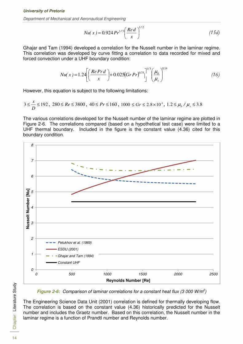
The various correlations developed for the Nusselt number of the laminar regime are plotted in Figure 2-6. The correlations compared (based on a hypothetical test case) were limited to a UHF thermal boundary. Included in the figure is the constant value (4.36) cited for this boundary condition.
Figure 2-6: Comparison of laminar correlations for a constant heat flux (3 000 W/m2)
The Engineering Science Data Unit (2001) correlation is defined for thermally developing flow. The correlation is based on the constant value (4.36) historically predicted for the Nusselt number and includes the Graetz number. Based on this correlation, the Nusselt number in the laminar regime is a function of Prandtl number and Reynolds number.
0
1
2
3
4
5
6
7
8
0 500 1000 1500 2000 2500
Nu
sselt
Nu
mb
er
[Nu
]
Reynolds Number [Re]
Petukhov et al. (1969)
ESDU (2001)
Ghajar and Tam (1994)
Constant UHF

Analysis of Theoretical Heat Transfer Coefficients for Laminar to Turbulent Flow in Smooth Tubes
Melissa Hallquist
Chapte
r: L
itera
ture
Stu
dy
15
As the flow rate increases, the fluid temperature would decrease, which results in an increase in the Prandtl number. This explains the increase in the Nusselt number predicted by the ESDU correlation as the flow approaches transition.
The Ghajar and Tam (1994) correlation is subject to a number of restrictions, but has been included in the figure for comparative purposes. The Nusselt number predicted with this correlation decreases up to a Reynolds number of approximately 1 300 where it stabilises to a value of approximately 6.37. As the flow approaches transition, the Nusselt number starts to increase.
The initial decrease in the Nusselt number is attributed to the influence of the Grashoff number included in the correlation. The Grashoff number depends on the temperature differential between the wall and the fluid, which increases as the flow rate decreases. The inclusion of the viscosity ratio results in higher Nusselt numbers in comparison with the other correlation results.
The subsequent increase in the Nusselt number is governed by the Reynolds number and Prandtl number as seen with the use of the ESDU correlation.
The Petukhov and Polyakov (1969) correlation shows a similar trend to the Ghajar and Tam (1994) correlation with the Nusselt number first decreasing as the Reynolds number increases. Based on this correlation, the Nusselt number is a function of the Grashoff number and the Prandtl number. As with the Ghajar and Tam (1994) correlation, the initial behaviour of the Nusselt number is due to the inclusion of the Grashoff number.
The Nusselt numbers are consistently lower than those predicted by Ghajar and Tam (1994), and do not show any increase as the flow approaches transition. The lower values are due to the absence of the viscosity ratio, and without including the Graetz number in this correlation, the values are not expected to increase.
It should be noted that the Petukhov et al. (1969) correlation is the only “average correlation” (giving the average Nusselt number and not the local value) in this section. All the other equations are originally cited for the local Nusselt number and therefore need to be integrated over the length of the tube in order to determine the average Nusselt number.
2.4.2 TURBULENT FLOW
For turbulent flow, a number of papers were written in order to describe the Nusselt number as a function of both Reynolds number and Prandtl number for the application of heat transfer in a tube.
The Chilton and Colburn analogy gives the Nusselt number for turbulent flow in smooth tubes (Cengel 2006) as follows:
311250
/PrRef.Nu = (17a)
The limitations of this equation are as follows: Re > 10 000, 0.7 < Pr < 160.
The friction factor for this correlation is based on the explicit first Petukhov equation:
( ) 2641790
−−= .Reln.f (17b)
This equation is valid for a Reynolds range of 63105103 .Re. <<

University of Pretoria
Department of Mechanical and Aeronautical Engineering
Chapte
r: L
itera
ture
Stu
dy
16
This correlation was modified in 1930 to resemble a more accurate form of the equation known as the Dittus and Boelter equation, which is still a popular correlation today:
n.PrRe.Nu
800230= (18)
The constant n is equal to 0.3 for cooling and 0.4 for heating and the limitations of the equation are: 2 500 < Re < 124 000, 0.7 < Pr < 120.
These equations were deemed acceptable to use when the temperature difference between the fluid and the wall surface was not too large. Sieder and Tate (1936) developed a relationship in 1936 taking into account the variation in fluid properties that could arise if this temperature difference was large (Cengel 2006; Kreith & Bohn 2001):
140
31800270
.
s
b/.PrRe.Nu
=
µ
µ (19)
The correlation developed by Sieder and Tate (1936) was based on an experimental set-up that approximated a constant wall temperature boundary condition. The limitations of the equation are as follows: Re > 10 000, 0.7 < Pr < 17 600
Hausen (Cengel 2006) developed a correlation that takes into account thermal effects of the entrance of the heat exchanger:
( )
+−=
32
42075011800370
/
..
d
xPrRe.)x(Nu (20)
Petukhov developed a relationship that is more complex than the above relationships, but is considered to be more accurate (Cengel 2006). It is known as the second Petukhov equation and is used in conjunction with the first Petukhov equation (17b) for the friction factor:
( )( ) ( )18712071
83250−+
=/.
Pr/f..
PrRe/fNu (21)
The correlation is only valid for the following ranges: 104 < Re < 5.10
6, 0.5 < Pr < 2 000.
This equation was then modified and improved on by Gnielinski in 1976 in order to make the relationship more accurate at lower Reynolds numbers (Cengel 2006):
( )( )( ) ( )187121
100083250−+
−=
/.Pr/f.
PrRe/fNu (22)
The correlation is only valid for the following ranges: 3.103 < Re < 5.10
6, 0.5 < Pr < 2 000
The corresponding friction factor equation is the first Petukhov equation (17b).
A report by the Engineering Sciences Data Unit (1993) gives a correction to the Petukhov equation which is valid for a wider range of Reynolds numbers (4 000 < Re < 5.10
6):
( )( )( ) ( )1821
100083250−+
−=
/.Pr/fKK
PrRe/fNu (23a)

Analysis of Theoretical Heat Transfer Coefficients for Laminar to Turbulent Flow in Smooth Tubes
Melissa Hallquist
Chapte
r: L
itera
ture
Stu
dy
17
where the corresponding constants are calculated as:
fK 6.1311 +=
3/1Pr8.17.112
−+=K
The friction factor to be used is:
( ) 2641821
−−= .Relog.f (23b)
The Churchill (1977) correlation for the turbulent regime is given as follows:
( )
( ) 6554
21
0
1
80790//
/
Pr
PrRe/f.NuNu
+= (24)
Nu0 is dependent on the thermal boundary condition, which is set to 4.8 for a uniform wall temperature boundary and 6.3 for a uniform heat flux boundary condition.
One of the more recent additions to the turbulent flow correlations is that of Ghajar and Tam (1994), which is applicable to turbulent forced convection in the entrance and fully developed flow regions. The correlation can be used for any inlet configuration and based on their experiments, Ghajar and Tam found a 10% error with the experimental data as follows:
14000540
3850800230
.
s
b
.
..
xd
xPrRe.Nu
=
−
µ
µ (25)
The correlation is only valid for the following parameter ranges: 1923 ≤≤ d/x , 344 ≤≤ Pr ,
490007000 ≤≤ Re , 7111 ./. sb ≤≤ µµ
2.4.3 TRANSITIONAL FLOW
According to a report by the Engineering Sciences Data Unit (1993), it is very difficult to predict the Nusselt number in the transitional regime because essentially, the transitional regime has aspects of both laminar and turbulent flow. However, one would expect the transitional Nusselt number to lie in the range between the limits of laminar and turbulent flow. An interpolation function is therefore suggested to determine the Nusselt number in this region:
( ) tl NuNuNu εε −+= 1 (26a)
where:
6000331
Re. −=ε (26b)
Despite the difficulties associated with the transitional flow regime, Churchill (1977) and Ghajar and Tam (1994) developed correlations that would cover the entire flow regime including transitional flow.

University of Pretoria
Department of Mechanical and Aeronautical Engineering
Chapte
r: L
itera
ture
Stu
dy
18
The Churchill correlation for the transitional regime is dependent on the laminar and turbulent Nusselt number correlations from the same author as follows:
( ) ( )
1015
2
655402
10
1
0790365
2200/
//c,l
l
Pr
PrfRe.Nu
Nu
Reexp
NuNu
+++
−
+=
−
−
(27)
Ghajar and Tam (1994) investigated the influence for the inlet configuration on heat transfer and came up with the following results:
( )c
c
tlx Nub
ReaexpNuNu
+
−+= (28)
Table 2-2: Constants and limitations for equation 27 (Ghajar & Tam 1994)
Inlet a b c Limitations
Re-entrant 1766 276 -0.955
1923 ≤≤ d/x
91001700 ≤≤ Re
515 ≤≤ Pr
510124000 ×≤≤ .Gr
2221 ./. sb ≤≤ µµ
Square-edged 2617 207 -0.950
1923 ≤≤ d/x
107001600 ≤≤ Re
555 ≤≤ Pr
510524000 ×≤≤ .Gr
6221 ./. sb ≤≤ µµ
Bellmouth 6628 237 -0.980
1923 ≤≤ d/x
111003300 ≤≤ Re
7713 ≤≤ Pr
510116000 ×≤≤ .Gr
1321 ./. sb ≤≤ µµ
Some of the correlations for the Nusselt number discussed in this chapter are compared (based on the same hypothetical test case used for the laminar correlations) with one another in Figure 2-7. The Nusselt numbers are plotted as a function of Reynolds number ranging from 500 to 15 000. These values are plotted for a hypothetical case of an 8 mm tube subject to a constant heat flux of 3 000 W/m2.
The accepted boundary for the onset of turbulence is at a Reynolds number of 2 300. However, very few of the correlations are valid at this low range, in fact many of them are only valid for Reynolds numbers larger than 10 000.

Analysis of Theoretical Heat Transfer Coefficients for Laminar to Turbulent Flow in Smooth Tubes
Melissa Hallquist
Chapte
r: L
itera
ture
Stu
dy
19
The ESDU (2001) correlation for transition flow is an interpolative correlation that has been determined using the ESDU correlation for laminar flow and the Gnielinski (1976) correlation for turbulent flow. The transitional Nusselt numbers follow on smoothly from the laminar results but are much lower than expected. The gradient of transition is expected to be steeper and this correlation still results in a discontinuity between transition and turbulent flow.
The Churchill (1977) correlation is developed across the entire Reynolds number range and makes provision for different thermal boundary conditions in the laminar regime as well as the transitional regime. The transitional results produced values that were not within the real number range and therefore could not be plotted.
The turbulent correlation is fairly well correlated, with predictions very close to the Petukhov correlation. The form of the equation is similar to the Petukhov correlation with the Nusselt number described as a function of the friction factor, Reynolds number and Prandtl number. No provision is made for secondary flow effects by the inclusion of either the Grashoff number or a viscosity ratio factor.
Figure 2-7: Nusselt number correlations for laminar to turbulent flow (3 000 W/m2)
The Ghajar and Tam (1994) correlation is also developed across all flow regimes, but is highly dependent on the inlet configuration with a number of limitations. The correlation plotted in the figure is that for a re-entrant inlet, which is the closest approximation to the current study. The transition between laminar and turbulent flow is relatively smooth with a small “jump” at the onset of transition and turbulent flow.
This correlation is originally developed for the local Nusselt number and must be numerically integrated to be compared with the other correlations. The correlation takes on the same form
0
20
40
60
80
100
120
140
0 2000 4000 6000 8000 10000 12000 14000 16000
Nu
sselt
Nu
mb
er
[Nu
]
Reynolds Number [Re]
Petukhov et al. (1969)
ESDU (2001)
Ghajar and Tam (1994)
Chilton and Colburn (1933)
Dittus and Boelter (1930)
Petukhov (1959)
Gnielinski (1976)
Churchill (1977)
Constant UHF
Colburn (1933)

University of Pretoria
Department of Mechanical and Aeronautical Engineering
Chapte
r: L
itera
ture
Stu
dy
20
as the Sieder and Tate equation with the addition of a local tube position factor (x/d). The viscosity ratio accounts for secondary flow effects, which explains the higher prediction seen at the onset of turbulent flow. This correlation does not include the effect of the friction losses in the tube.
The Gnielinski (1976) correlation is very similar to the Petukhov (1969) correlation with much lower Nusselt number predictions. These correlations are mainly dependent on the friction factor and the Gnielinski correlation is a favoured correlation due to the wide Reynolds number range applicable. These correlations do not take any secondary flow effects into account.
For easy reference, a summary of all the correlations and their limitations is given in Table 2-3.

Analysis of Theoretical Heat Transfer Coefficients for Laminar to Turbulent Flow in Smooth Tubes
Melissa Hallquist
Chapte
r: L
itera
ture
Stu
dy
21
Table 2-3: Summary of Nusselt number correlations
Inlet Correlation Flow Regime Boundary Limitation
Petukhov et al. (1969)
04504
180001364
.
Ra.Nu
+= Laminar Flow
ESDU (2001) ( )[ ] 31331337077170663
//
.Gz...Nu −++= Laminar Flow UWT Thermally Developing
ESDU (2001) ( )[ ] 31331360117213644
//
.Gz..Nu −++= Laminar Flow UWT Thermally Developing
ESDU (2001) ( )31
21
6133133
221
247075170663
/
/
/
/Gz
Pr.Gz...Nu
++−++=
π Laminar Flow UHF Simultaneously Developing
ESDU (2001)
21
319240
/
/
x
dRePr.)x(Nu
= Laminar Flow UHF Simultaneously Developing
Ghajar and Tam (1994)
( )14031
7500250241
.
s
b
/
.PrGr.
x
dPrRe.)x(Nu
+
=
µ
µ Laminar Flow UHF
1923 ≤≤D
x
3800Re280 ≤≤
160Pr40 ≤≤ 4
108.21000 ×≤≤ Gr
8.32.1 ≤≤w
b
µ
µ
Churchill (1977)
=
UWTfor.
UHFfor.Nu
6573
3644 Laminar Flow

University of Pretoria
Department of Mechanical and Aeronautical Engineering
Chapte
r: L
itera
ture
Stu
dy
22
Colburn and du Pont de (1933)
311250
/PrRef.Nu = Turbulent Flow Re > 10000
0.7 < Pr < 160
Dittus and Boelter (1930)
n.PrRe.Nu
800230= Turbulent Flow UHF
2500< Re < 124 000 0.7 < Pr < 120
Sieder and Tate (1936)
140
31800270
.
s
b/.PrRe.Nu
=
µ
µ Turbulent Flow UWT
Re > 10000 0.7 < Pr < 17600
Hausen (1959) ( )
+−=
32
42075011800370
/
..
d
xPrRe.)x(Nu Turbulent Flow
First Petukhov (1970)
( )( ) ( )18712071
83250−+
=/.
Pr/f..
PrRe/fNu Turbulent Flow
104 < Re < 5.106 0.5 < Pr < 2000
Corrected Petukhov
( )( ) ( )18712071
83250−+
=/.
Pr/f..
PrRe/fNu Turbulent Flow
4000 < Re < 5.106 0.5 < Pr < 2000
Gnielinski (1976)
( )( )( ) ( )187121
100083250−+
−=
/.Pr/f.
PrRe/fNu Turbulent Flow
3.103 < Re < 5.106 0.5 < Pr < 2000
Churchill (1977)
( )( ) 6554
21
0
1
80790//
/
Pr
PrRe/f.NuNu
+= Turbulent Flow
Ghajar and Tam (1994)
14000540
3850800230
.
s
b
.
..
d
xPrRe.)x(Nu
=
−
µ
µ Turbulent Flow UHF
1923 ≤≤D
x
49000Re7000 ≤≤
34Pr4 ≤≤
7.11.1 ≤≤w
b
µ
µ

Analysis of Theoretical Heat Transfer Coefficients for Laminar to Turbulent Flow in Smooth Tubes
Melissa Hallquist
Chapte
r: L
itera
ture
Stu
dy
23
ESDU (2001) ( ) tl NuNuNu εε −+= 1 Transitional
Flow -
Churchill (1977) ( ) ( )
1015
2
655402
10
1
0790385
2200/
//c,l
l
Pr
PrfRe.Nu
Nu
Reexp
NuNu
+++
−
+=
−
−
Transitional Flow
Ghajar and Tam (1994)
( )c
c
tl Nub
ReaexpNuNu
+
−+=
Transitional Flow
UHF Inlet Configuration

University of Pretoria
Department of Mechanical and Aeronautical Engineering
Chapte
r: L
itera
ture
Stu
dy
24
2.5 ENTRANCE REGION AND ENTRANCE EFFECTS
As can be seen in Figure 2-8, the velocity profile of fluid flowing through a tube develops from the entrance of the tube in various stages before it resembles fully laminar and eventually turbulent flow.
v v v v v
Figure 2-8: The development of the velocity profile in a circular tube (Cengel 2006)
Initially the leading profile of the fluid is fairly flat, but due to viscous shearing the velocity of the fluid directly adjacent to the tube wall becomes zero. This area of zero velocity is known as the velocity boundary layer. The motionless layer at the edge of the tube wall slows down the particles adjacent to it until the profile of the fluid resembles a parabola, as illustrated in Figure 2-8.
This profile is characteristic of Poiseuille flow, as described in Mills (1992). At this point, the flow is characterised as fully developed laminar flow. Most of the relationships that describe the heat transfer of fluid flow are only applicable when the flow is hydrodynamically fully developed. The subsequent velocity used in all calculations is the average velocity, which remains constant throughout the tube for steady incompressible flow.
In a similar manner, if a fluid at a uniform temperature enters a tube with a different surface temperature the fluid also develops a thermal profile (Cengel 2006). The fluid particles in direct contact with the wall of the tube assume the surface temperature, which initiates convection heat transfer in the tube. The layer of fluid directly adjacent to the tube wall is known as the thermal boundary layer. The thermal profile that results closely resembles a parabola, which is shown in Figure 2-9, and at this point, the fluid is known as thermally fully developed flow.
In the case of laminar flow in a tube, the thermal boundary layer extends to the centre line of the tube, and its thickness is independent of the velocity. Therefore, the temperature gradient at the wall and the heat transfer coefficient is also independent of velocity. In the case of turbulent flow, the increase in velocity results in a dynamic mixing in the core flow of the tube. This in turn allows for an increase in the heat transfer coefficient and a consequent thinning of the viscous layer adjacent to the wall of the tube (Mills 1992).
It is vital that fluid flow reaches these fully developed regions for efficient heat exchange to take place. If the fluid is thermally fully developed, the local convection coefficient remains constant. Likewise, if the flow is hydrodynamically fully developed, the friction coefficient remains constant. This allows for more accurate calculations. According to Mills (1992), the hydrodynamic entrance length can be defined as the distance required for the friction factor to
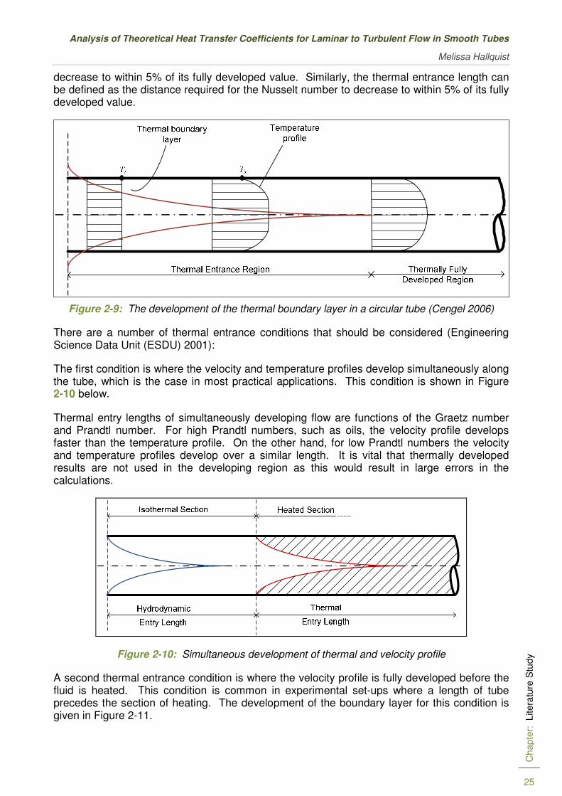
Analysis of Theoretical Heat Transfer Coefficients for Laminar to Turbulent Flow in Smooth Tubes
Melissa Hallquist
Chapte
r: L
itera
ture
Stu
dy
25
decrease to within 5% of its fully developed value. Similarly, the thermal entrance length can be defined as the distance required for the Nusselt number to decrease to within 5% of its fully developed value.
Figure 2-9: The development of the thermal boundary layer in a circular tube (Cengel 2006)
There are a number of thermal entrance conditions that should be considered (Engineering Science Data Unit (ESDU) 2001):
The first condition is where the velocity and temperature profiles develop simultaneously along the tube, which is the case in most practical applications. This condition is shown in Figure 2-10 below.
Thermal entry lengths of simultaneously developing flow are functions of the Graetz number and Prandtl number. For high Prandtl numbers, such as oils, the velocity profile develops faster than the temperature profile. On the other hand, for low Prandtl numbers the velocity and temperature profiles develop over a similar length. It is vital that thermally developed results are not used in the developing region as this would result in large errors in the calculations.
Figure 2-10: Simultaneous development of thermal and velocity profile
A second thermal entrance condition is where the velocity profile is fully developed before the fluid is heated. This condition is common in experimental set-ups where a length of tube precedes the section of heating. The development of the boundary layer for this condition is given in Figure 2-11.
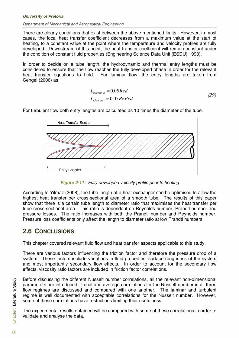
University of Pretoria
Department of Mechanical and Aeronautical Engineering
Chapte
r: L
itera
ture
Stu
dy
26
There are clearly conditions that exist between the above-mentioned limits. However, in most cases, the local heat transfer coefficient decreases from a maximum value at the start of heating, to a constant value at the point where the temperature and velocity profiles are fully developed. Downstream of this point, the heat transfer coefficient will remain constant under the condition of constant fluid properties (Engineering Science Data Unit (ESDU) 1993).
In order to decide on a tube length, the hydrodynamic and thermal entry lengths must be considered to ensure that the flow reaches the fully developed phase in order for the relevant heat transfer equations to hold. For laminar flow, the entry lengths are taken from Cengel (2006) as:
dPrRe.L
dRe.L
arminla,t
arminla,h
050
050
=
= (29)
For turbulent flow both entry lengths are calculated as 10 times the diameter of the tube.
Figure 2-11: Fully developed velocity profile prior to heating
According to Yilmaz (2008), the tube length of a heat exchanger can be optimised to allow the highest heat transfer per cross-sectional area of a smooth tube. The results of this paper show that there is a certain tube length to diameter ratio that maximises the heat transfer per tube cross-sectional area. This ratio is dependent on Reynolds number, Prandtl number and pressure losses. The ratio increases with both the Prandtl number and Reynolds number. Pressure loss coefficients only affect the length to diameter ratio at low Prandtl numbers.
2.6 CONCLUSIONS
This chapter covered relevant fluid flow and heat transfer aspects applicable to this study.
There are various factors influencing the friction factor and therefore the pressure drop of a system. These factors include variations in fluid properties, surface roughness of the system and most importantly secondary flow effects. In order to account for the secondary flow effects, viscosity ratio factors are included in friction factor correlations.
Before discussing the different Nusselt number correlations, all the relevant non-dimensional parameters are introduced. Local and average correlations for the Nusselt number in all three flow regimes are discussed and compared with one another. The laminar and turbulent regime is well documented with acceptable correlations for the Nusselt number. However, some of these correlations have restrictions limiting their usefulness.
The experimental results obtained will be compared with some of these correlations in order to validate and analyse the data.

Analysis of Theoretical Heat Transfer Coefficients for Laminar to Turbulent Flow in Smooth Tubes
Melissa Hallquist
Chapte
r:
Experi
menta
l P
rocedure
27
3. EXPERIMENTAL PROCEDURE
3.1 INTRODUCTION
This chapter describes all the aspects of the experimental procedure followed in this study. An overview of the experimental set-up is presented including the overall set-up, the removable test section as well as the controller, which ensures the uniform heat flux boundary. The measurement procedure and equipment used to conduct the experiments are described before a detailed data reduction is presented. The data reduction describes the method used to determine the different Nusselt numbers and friction factors from the measurements taken. A summary of the expected uncertainties is included, paying attention to the inherent measurement errors of the instruments, uncertainties of the fluid properties determined and the various calculated parameters. The measurements are validated by comparing them against literature before concluding this chapter.
3.2 EXPERIMENTAL SET-UP
The experimental set-up can be divided into three main sections, namely the overall set-up, the test section and the control system, which maintained a predetermined heat flux boundary condition on a test section through which water flows.
3.2.1 OVERALL SET-UP
The overall test set-up (Figure 3-1) consisted of a closed water loop, which circulated water from a storage tank through a removable test section back to the storage tank. This test section was set up to accommodate test tubes of different diameters and lengths. Various heating fluxes could be applied to the test section by passing different currents through the test tubes.
Figure 3-1: Process Diagram for Test Set-up
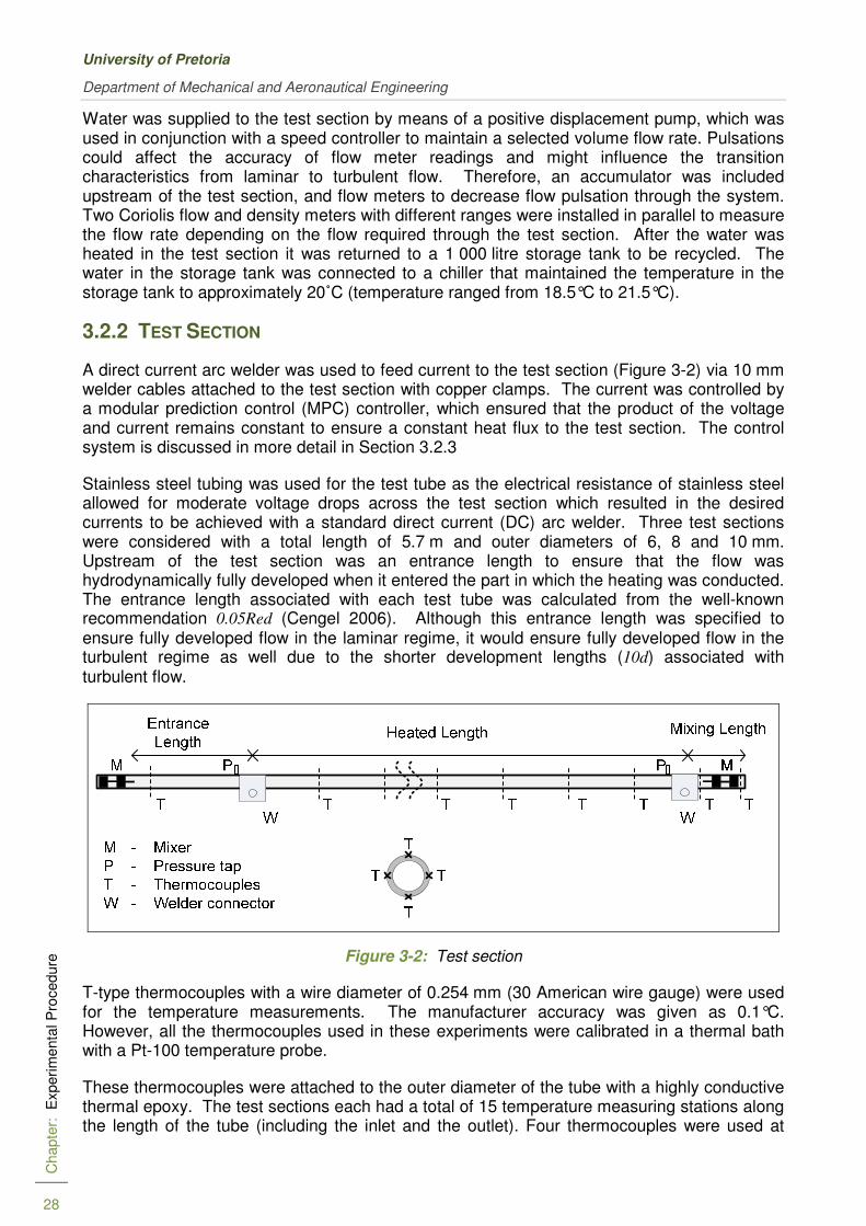
University of Pretoria
Department of Mechanical and Aeronautical Engineering
Chapte
r:
Experi
menta
l P
rocedure
28
Water was supplied to the test section by means of a positive displacement pump, which was used in conjunction with a speed controller to maintain a selected volume flow rate. Pulsations could affect the accuracy of flow meter readings and might influence the transition characteristics from laminar to turbulent flow. Therefore, an accumulator was included upstream of the test section, and flow meters to decrease flow pulsation through the system. Two Coriolis flow and density meters with different ranges were installed in parallel to measure the flow rate depending on the flow required through the test section. After the water was heated in the test section it was returned to a 1 000 litre storage tank to be recycled. The water in the storage tank was connected to a chiller that maintained the temperature in the storage tank to approximately 20˚C (temperature ranged from 18.5°C to 21.5°C).
3.2.2 TEST SECTION
A direct current arc welder was used to feed current to the test section (Figure 3-2) via 10 mm welder cables attached to the test section with copper clamps. The current was controlled by a modular prediction control (MPC) controller, which ensured that the product of the voltage and current remains constant to ensure a constant heat flux to the test section. The control system is discussed in more detail in Section 3.2.3
Stainless steel tubing was used for the test tube as the electrical resistance of stainless steel allowed for moderate voltage drops across the test section which resulted in the desired currents to be achieved with a standard direct current (DC) arc welder. Three test sections were considered with a total length of 5.7 m and outer diameters of 6, 8 and 10 mm. Upstream of the test section was an entrance length to ensure that the flow was hydrodynamically fully developed when it entered the part in which the heating was conducted. The entrance length associated with each test tube was calculated from the well-known recommendation 0.05Red (Cengel 2006). Although this entrance length was specified to ensure fully developed flow in the laminar regime, it would ensure fully developed flow in the turbulent regime as well due to the shorter development lengths (10d) associated with turbulent flow.
Figure 3-2: Test section
T-type thermocouples with a wire diameter of 0.254 mm (30 American wire gauge) were used for the temperature measurements. The manufacturer accuracy was given as 0.1°C. However, all the thermocouples used in these experiments were calibrated in a thermal bath with a Pt-100 temperature probe.
These thermocouples were attached to the outer diameter of the tube with a highly conductive thermal epoxy. The test sections each had a total of 15 temperature measuring stations along the length of the tube (including the inlet and the outlet). Four thermocouples were used at
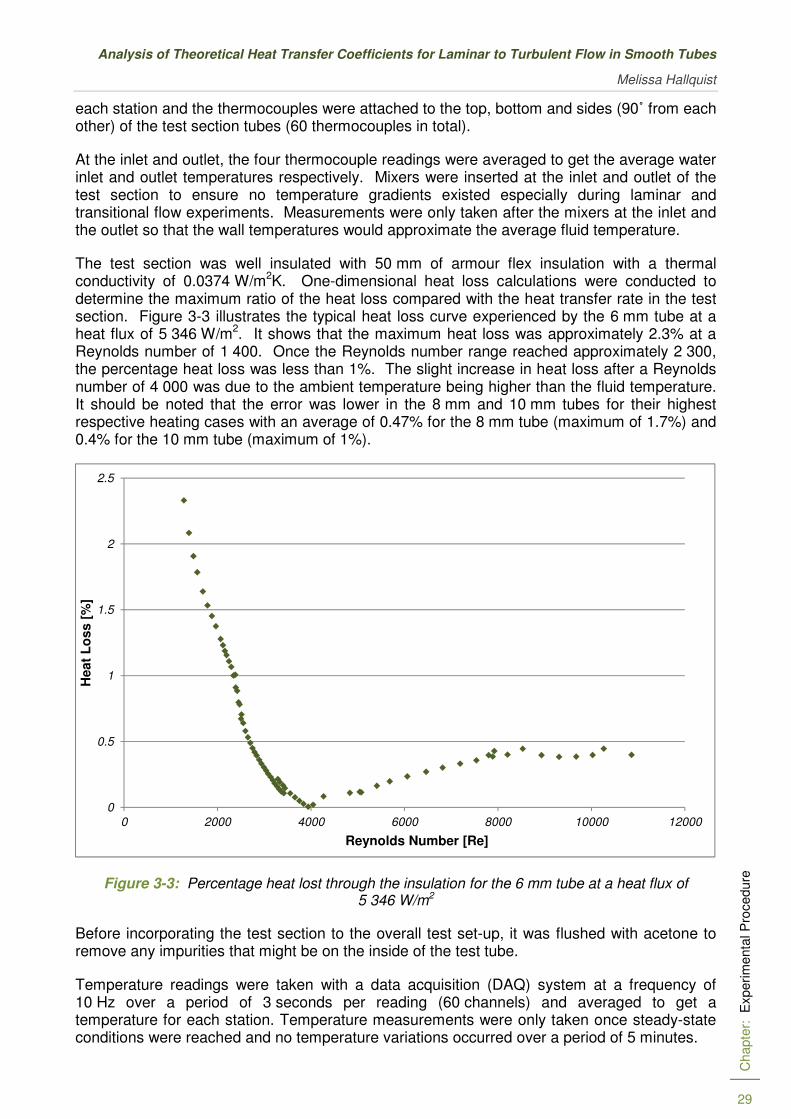
Analysis of Theoretical Heat Transfer Coefficients for Laminar to Turbulent Flow in Smooth Tubes
Melissa Hallquist
Chapte
r:
Experi
menta
l P
rocedure
29
each station and the thermocouples were attached to the top, bottom and sides (90˚ from each other) of the test section tubes (60 thermocouples in total).
At the inlet and outlet, the four thermocouple readings were averaged to get the average water inlet and outlet temperatures respectively. Mixers were inserted at the inlet and outlet of the test section to ensure no temperature gradients existed especially during laminar and transitional flow experiments. Measurements were only taken after the mixers at the inlet and the outlet so that the wall temperatures would approximate the average fluid temperature.
The test section was well insulated with 50 mm of armour flex insulation with a thermal conductivity of 0.0374 W/m2K. One-dimensional heat loss calculations were conducted to determine the maximum ratio of the heat loss compared with the heat transfer rate in the test section. Figure 3-3 illustrates the typical heat loss curve experienced by the 6 mm tube at a heat flux of 5 346 W/m2. It shows that the maximum heat loss was approximately 2.3% at a Reynolds number of 1 400. Once the Reynolds number range reached approximately 2 300, the percentage heat loss was less than 1%. The slight increase in heat loss after a Reynolds number of 4 000 was due to the ambient temperature being higher than the fluid temperature. It should be noted that the error was lower in the 8 mm and 10 mm tubes for their highest respective heating cases with an average of 0.47% for the 8 mm tube (maximum of 1.7%) and 0.4% for the 10 mm tube (maximum of 1%).
Figure 3-3: Percentage heat lost through the insulation for the 6 mm tube at a heat flux of 5 346 W/m2
Before incorporating the test section to the overall test set-up, it was flushed with acetone to remove any impurities that might be on the inside of the test tube.
Temperature readings were taken with a data acquisition (DAQ) system at a frequency of 10 Hz over a period of 3 seconds per reading (60 channels) and averaged to get a temperature for each station. Temperature measurements were only taken once steady-state conditions were reached and no temperature variations occurred over a period of 5 minutes.
0
0.5
1
1.5
2
2.5
0 2000 4000 6000 8000 10000 12000
Heat
Lo
ss [
%]
Reynolds Number [Re]

University of Pretoria
Department of Mechanical and Aeronautical Engineering
Chapte
r:
Experi
menta
l P
rocedure
30
Pressure taps were connected to a pressure transducer in order to determine the friction factor of the heated length of the test section. These pressure taps were attached to the tube just before heat was applied at the inlet and just before removing heat at the outlet. The hole for the pressure tap measured a maximum of 0.4 mm, which was less than 10% of the tube diameter, as suggested by Rayle (1959). Once the taps were attached to the test tube, the inner-tube diameter was sanded to ensure that there were no burrs on the surface of the pressure taps.
A T-140 Beta pressure calibrator was connected to the test section in parallel with a DP15 pressure transducer. Connection with the test section was achieved with 2 mm plastic tubing, which was inserted into pneumatic connectors screwed into compression fittings attached to the taps of the test section. To ensure accurate readings, the tubing had to be coiled and fastened to the test bench to avoid any kinks that could affect the results.
The DP15 transducer was incorporated into the same DAQ system as the thermocouples so that simultaneous readings could be taken. The T-140 calibrator was used to monitor the pressure of the system and ensure that the readings taken by the DP15 were accurate. The full-scale accuracy of this transducer was 0.25% of the full-scale value.
Before connecting the pressure transducer to the test section, each of the diaphragms used was calibrated on a water column. Once incorporated into the test section, water was pumped through the system and all the tubes were bled of air. The bypass valve was opened to simulate a zero pressure condition for the system. This zero was compared with the calibrated zero and the offset measured.
3.2.3 CONTROL SYSTEM
In order to maintain a constant heat flux boundary condition for the test set-up, a control system was developed that controlled the root mean square average of the product of the voltage supplied (V) to the system and the current being drawn (i). The control measurement system comprised of a digital acquisition device (DAQ) and circuitry for conditioning, measurement and driver capability.
The digital acquisition device was a 16-bit analogue to digital conversion (A/DC) and a 12-bit digital to analogue conversion (D/AC) device, which was controlled via dedicated microcontroller hardware consisting of the following: a liquid crystal display (LCD) that indicated the power being delivered to the system as a function of the root mean square voltage and current. The controller was designed as a model predictive control (MPC) system. This required power to be selected before the current source could be applied. The actual control mechanism was proportional integral derivative (PID) control with a settling time (ts) of 0.2 ms, an offset error of 0.1% and a peak overshoot of 2%.
Pulse width modulation (PWM) was used in order to maintain the correct current driving capability on the power source. Switching frequencies were selected to be higher than the sampling frequencies in order to prevent “noise” being associated with the measurement.
A simple operation flow diagram is given in Figure 3-4 to illustrate the basic function of the controller.
The current supplied by the welder was switched on and off by an insulated gate bipolar transistor (IGBT) bridge to reduce the current to desired levels. The current and voltage supplied to the test section (device under test) were monitored by sensors so that the control device could compensate if the values were too high. There were filters that counteract aliasing to eliminate noise in the current and voltage signals being measured. The analogue to digital (A/D) channel converted the analogue value to a digital one that could be used by the

Analysis of Theoretical Heat Transfer Coefficients for Laminar to Turbulent Flow in Smooth Tubes
Melissa Hallquist
Chapte
r:
Experi
menta
l P
rocedure
31
digital control system. Root mean square (RMS) values of the current and voltage were used to determine the actual power being delivered to the system.
The control action look-up determined the maximum amount of duty cycle that might be moved by the system without damaging the IGBT bridge. A PID control loop ensured that the output value did not overshoot the desired values and that the control system settled quickly. If the current needed to be modified, the PWM had to be adjusted in order to get the proportional current value out. A driver circuit was included in order to drive the IGBT to saturation in order for the IGBT to switch ON.
Figure 3-4: Flow diagram for the operation of the control system

University of Pretoria
Department of Mechanical and Aeronautical Engineering
Chapte
r:
Experi
menta
l P
rocedure
32
3.3 EXPERIMENTAL PROCEDURE
3.3.1 MEASUREMENT PROCEDURE
The main objective of the experiment was to obtain the necessary data to determine the heat transfer coefficients and friction factors for different tube diameters over the transitional flow region by applying different heat fluxes. Municipal water and not distilled water was used to conduct the experiments as no fouling problems were experienced. This was also observed by other researchers (Meyer & Du Preez 2010; Olivier & Meyer 2010; Sulliman, Liebenberg & Meyer 2009; Van Rooyen et al. 2010) in the same laboratory using the same water supply.
The experiments covered the Reynolds number range of 450 to 10 000, the Prandtl number range of 4 to 7, the Nusselt number range of 4 to 130, and the Grashoff number range of 40 to 1 100 depending on the test section being investigated. The wall heat flux of the experiments ranged from 1 200 to 6 300 W/m2. The measurement intervals were more concentrated around the transition region (2 000 < Re <4 000) and widely spaced in the turbulent region.
To increase the accuracy of the pressure readings, different diaphragms were inserted into the pressure transducer with different pressure ranges as the mass flow through the tube was changed. This ensured the best resolution on the pressure reading measurements. The readings for each diaphragm overlapped one another by a few points to ensure consistency of the results.
For each diaphragm, the flow rate to be tested was set before the electrical current was applied to the test section, which transferred the electrical heat to the water flowing through the tube. The system was first given time to reach steady-state conditions before the temperature and pressure drop readings were taken. While the heat flux to the test section was kept constant, the mass flow rate was changed and another set of readings was taken. Once readings were taken for a full range of flow rates per diaphragm, the heat flux was changed and the process was repeated.
3.3.2 DATA REDUCTION
Heat transfer was achieved through the heating effect of the electrical power (elec
.
Q ) delivered
to the system, which was determined from the measured current (i) and the electrical resistance (R) of the test section as follows:
RiQ.
elec
2= (30)
The electrical resistance (R) of the test section was determined by the following correlation which is a function of the average test section temperature and the temperature coefficient (α) of stainless steel obtained from the material certificate of the supplier:
( )[ ]100 +−= TTRR α (31a)
where:
cA
LR σ=0
(31b)
The reference resistance (Ro) in the equation is the resistance at a temperature (To) of 20˚C, where L is the heated length of the test tube and A is the cross-sectional area of the tube material. To confirm the calculated resistance, a multimeter was attached to the copper

Analysis of Theoretical Heat Transfer Coefficients for Laminar to Turbulent Flow in Smooth Tubes
Melissa Hallquist
Chapte
r:
Experi
menta
l P
rocedure
33
clamps carrying current to the test section in order to measure the exact voltage drop across the stainless steel tube. A current probe was also used to confirm that the current measured with the controller was accurate. From this, the resistance could be calculated from:
iRV = (32)
The difference between the resistance calculated from the measured voltage and current, and the resistance based on the temperature calculation was approximately 0.05%.
The inside wall temperatures (Tsi) were determined by subtracting the temperature drop, as a result of the wall resistance, from the measurements of the outside wall temperatures (Tso):
thermal
.
elecsosi
R
QTT −= (33a)
where:
kL
)d/dln(R io
thermalπ2
= (33b)
The heat input from the electricity side (elec
.
Q ) was used in equation 33a because the local heat
input could be directly determined as opposed to the heat transfer on the water side, which is solely dependent on the inlet and outlet temperatures.
The wall thickness of the test sections was approximately 1 mm and thermal conductivity was quite high resulting in a maximum temperature drop of 0.33°C across the tube wall.
The average fluid temperature at any point, x, along the tube was determined from:
)x(Cm
xd)x(qT)x(T
p
.
i
i,ff
π+= (34)
where q(x) is determined from the local heat flux based on the current passing through the test section and the local electrical resistance R(x) between the inlet and point x. R(x) is determined from equation 31 where the temperature is the average wall temperature between the inlet and point x. Figure 3-5 illustrates an example where the station number was used for x.
The heat flux was determined as:
xd
xQxq
iπ
)()( = (35)
This equation is solved in an iterative manner where the specific heat is initially based on the average between the inlet temperature and the wall temperature at point x. Once the fluid temperature at position x has been calculated, the specific heat is adjusted according to this temperature until convergence has been achieved.

University of Pretoria
Department of Mechanical and Aeronautical Engineering
Chapte
r:
Experi
menta
l P
rocedure
34
Figure 3-5: Calculation of local fluid temperature
This process was repeated for each station after which the last element was compared with the actual measured outlet temperature. The difference between the numerical analysis and the measured temperature is directly related to the error between the power input to the system and the heat transfer between the water inlet and outlet. This error ranges from 2.4°C at low Reynolds numbers to 0.11°C at high Reynolds numbers.
The results of the calculated fluid temperature illustrated a straight line profile between inlet and calculated outlet as is expected for a constant heat flux boundary condition.
The tube inner-wall temperatures and the average fluid temperatures were used to determine the heat transfer coefficient and ultimately, the Nusselt number for each test case. There were three different types of Nusselt numbers that were considered in this study, namely a) the local Nusselt number as a function of the tube length, b) the average Nusselt number of the test section as a function of Reynolds number, c) the fully developed Nusselt number also as a function of Reynolds number.
The calculation of the three Nusselt number types is explained in more detail with reference to Figure 3-6, which gives the typical temperature distribution (Figure 3-6a) of the inner-wall temperature and the bulk fluid temperature at any station. It shows the part (Lh) before the test section in which the flow hydrodynamically gets fully developed before heating starts. Then the flow thermally develops (Lt) and during this part the temperature gradients of the wall and fluid are not the same. Figure 3-6c illustrates the typical local Nusselt number distribution. At the inlet, the local Nusselt number is at its highest and it decreases and flattens down and is constant from the point onwards when the flow is fully developed. When the flow is thermally (and hydrodynamically) fully developed, the temperature gradients of the wall and fluid are equal.
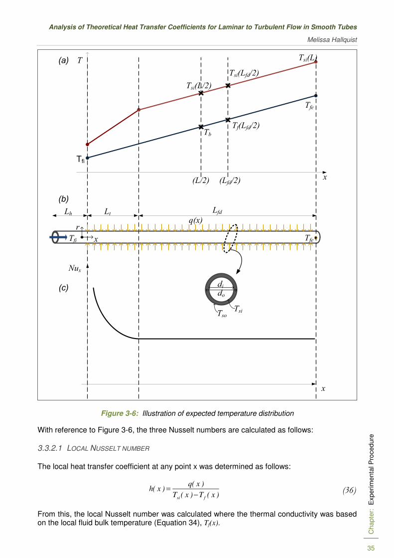
Analysis of Theoretical Heat Transfer Coefficients for Laminar to Turbulent Flow in Smooth Tubes
Melissa Hallquist
Chapte
r:
Experi
menta
l P
rocedure
35
Lh Ltq(x)
Tfe
Tfi
Tsi(L)
x
T
Tsi(L/2)
Tb
Nux
x
Tfi Tfe
r
x
Lfd
Tf(Lfd/2)
(L/2) (Lfd/2)
Tsi(Lfd/2)
(a)
(b)
(c)
Tsi
do
di
Tso
Figure 3-6: Illustration of expected temperature distribution
With reference to Figure 3-6, the three Nusselt numbers are calculated as follows:
3.3.2.1 LOCAL NUSSELT NUMBER
The local heat transfer coefficient at any point x was determined as follows:
)x(T)x(T
)x(q)x(h
fsi −= (36)
From this, the local Nusselt number was calculated where the thermal conductivity was based on the local fluid bulk temperature (Equation 34), Tf(x).

University of Pretoria
Department of Mechanical and Aeronautical Engineering
Chapte
r:
Experi
menta
l P
rocedure
36
)x(k
d)x(h)x(Nu i= (37)
The corresponding Reynolds number was based on the viscosity calculated at the local fluid temperature, Tf(x).
i
.
d)x(
m)xRe(
πµ
4= (38)
3.3.2.2 AVERAGE NUSSELT NUMBER
The average heat transfer coefficient for the entire test section was determined as:
bs
s
TT
qh
−=
(39)
The average wall temperature sT was determined by integrating the average of the 14
measurement stations along the length of the tube using the trapezoidal rule:
++= ∑13
2
141 222
1ssxss TTTT (40)
The bulk temperature in Equation 39 was determined as the average temperature between the fluid inlet bulk temperature and outlet bulk temperature, thus
2
fofi
b
TTT
−= (41)
The average Nusselt number was then determined as:
k
dhNu i= (42)
where the average thermal conductivity k was based on the bulk fluid temperature as calculated by Equation 46. The corresponding average Reynolds number was determined as:
i
.
d
meR
πµ
4= (43)
where the viscosity was determined at the bulk temperature (Equation 41).
3.3.2.3 FULLY DEVELOPED NUSSELT NUMBER
The fully developed heat transfer coefficients were determined as:
2/)()2/( fdffdsi
fdLTLT
qh
−= (44)
and the corresponding Nusselt number as
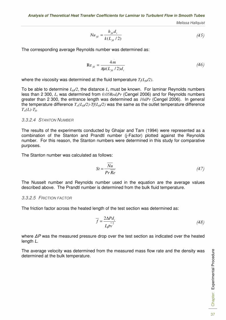
Analysis of Theoretical Heat Transfer Coefficients for Laminar to Turbulent Flow in Smooth Tubes
Melissa Hallquist
Chapte
r:
Experi
menta
l P
rocedure
37
)2/( fd
ifd
fdLk
dhNu =
(45)
The corresponding average Reynolds number was determined as:
ifd
fddL
m
)2/(
4Re
.
πµ=
(46)
where the viscosity was determined at the fluid temperature Tf(Lfd/2).
To be able to determine Lfd/2, the distance Lt must be known. For laminar Reynolds numbers less than 2 300, Lt was determined from 0.05RediPr (Cengel 2006) and for Reynolds numbers greater than 2 300, the entrance length was determined as 10dPr (Cengel 2006). In general the temperature difference Tsi(Lfd/2)-Tf(Lfd/2) was the same as the outlet temperature difference Tsi(L)-Tfe
3.3.2.4 STANTON NUMBER
The results of the experiments conducted by Ghajar and Tam (1994) were represented as a combination of the Stanton and Prandtl number (j-Factor) plotted against the Reynolds number. For this reason, the Stanton numbers were determined in this study for comparative purposes.
The Stanton number was calculated as follows:
RePr
NuSt = (47)
The Nusselt number and Reynolds number used in the equation are the average values described above. The Prandtl number is determined from the bulk fluid temperature.
3.3.2.5 FRICTION FACTOR
The friction factor across the heated length of the test section was determined as:
2
2
vL
Pdf i
ρ
∆= (48)
where ∆P was the measured pressure drop over the test section as indicated over the heated length L.
The average velocity was determined from the measured mass flow rate and the density was determined at the bulk temperature.

University of Pretoria
Department of Mechanical and Aeronautical Engineering
Chapte
r:
Experi
menta
l P
rocedure
38
3.4 UNCERTAINTIES
The uncertainties of the test set-up were calculated according to the method suggested in Kline and McClintock (1953). The uncertainty in a system is based on fixed errors and random errors known as the bias and precision respectively:
( ) ( ) 2122 /
iii pbx +=δ (49)
In the sections that follow, various errors that would affect the results of the experimental work are discussed. These errors include accuracy of the instruments used and uncertainties of calculated properties.
3.4.1 INSTRUMENTS
In the case of the instruments, the bias is considered as the accuracy specified by the manufacturer. The standard deviation of each instrument was measured across 100 points to be used as the precision error.
3.4.1.1 THERMOCOUPLES
The thermocouples were calibrated in a thermal bath with a Pt 100 temperature probe with a specified accuracy of 0.05°C. Thirty data points were taken between 20 and 75°C, and at each point, 50 readings were taken. Each of the channels were plotted against the measurements of the Pt 100 (channel 105 shown in Figure 3-7) and due to the highly linear relationship a first-order polynomial was fitted through all the points to obtain a calibration curve for each thermocouple.
After developing a calibration curve, the readings were adjusted according to this curve and again compared with the readings of the Pt 100. The average deviation between the adjusted measurements and the readings of the Pt 100 was 0.04°C. This error was added to the specified uncertainty of the Pt 100, resulting in an overall uncertainty of approximately 0.09°C (0.1°C) for each of the thermocouples.
To complete the uncertainty analysis, the standard deviation of each of the thermocouple data points was determined over 50 consecutive readings. On average, the standard deviation of the thermocouples was measured to be 0.02°C and therefore the total uncertainty was 0.102°C.

Analysis of Theoretical Heat Transfer Coefficients for Laminar to Turbulent Flow in Smooth Tubes
Melissa Hallquist
Chapte
r:
Experi
menta
l P
rocedure
39
Figure 3-7: Calibration curve for channel 105 in the 6 mm tube test case
3.4.1.2 PRESSURE TRANSDUCER
The pressure transducer (DP15 Validyne) has a number of different diaphragms that were used to improve the resolution of the readings. The following diaphragms were used for each test section:
Table 3-1: Diaphragm sizes used
Diaphragm
Size
Pressure
Rating (kPa)
6 mm
Test Case
8 mm
Test Case
10 mm
Test Case
22 2.2 X X
26 3.5 X
28 5.5 X X X
32 14 X X X
36 35 X
40 86 X
42 140 X
A 3 m water column was used to calibrate the diaphragms up to a pressure of 30 kPa. A T-140 calibrator was connected in parallel to the pressure transducer to measure the exact static pressure. At least 10 points were measured between zero and the maximum pressure rating of the diaphragm, where 50 readings were taken for each point. As with the thermocouples, the relationship between the pressure transducer and the calibration unit is highly linear. In
y = 1.00380x + 0.61071
0
10
20
30
40
50
60
70
80
0 10 20 30 40 50 60 70 80
Th
erm
oco
up
le (
105)
PT 100

University of Pretoria
Department of Mechanical and Aeronautical Engineering
Chapte
r:
Experi
menta
l P
rocedure
40
each case a first-order polynomial was curve fitted through the calibration points as shown in Figure 3-8.
Figure 3-8: Calibration curve for the pressure transducer
The accuracy of each diaphragm is specified as 0.25% of the full-scale value, which is considered as the bias. The precision is determined by the standard deviation of 100 readings. The results are given in the table below where the uncertainty is a combination of the bias and the precision given in Equation 49 (noting that the bias is 0.25% of the full-scale value).
Table 3-2: Expected uncertainty for each diaphragm
Diaphragm Size Bias Precision Uncertainty
22 0.25% 1.01% 1.04%
26 0.25% 1.03% 1.06%
28 0.25% 0.4% 0.47%
32 0.25% 0.55% 0.60%
36 0.25% 0.18% 0.31%
40 0.25% 0.45% 0.51%
42 0.25% 1.01% 1.04%
y = 1.0126x - 0.0242
0
1
2
3
4
5
6
0 1 2 3 4 5 6
Pre
ssu
re T
ran
sd
ucer
Read
ing
[kP
a]
Beta T140 Reading [kPa]
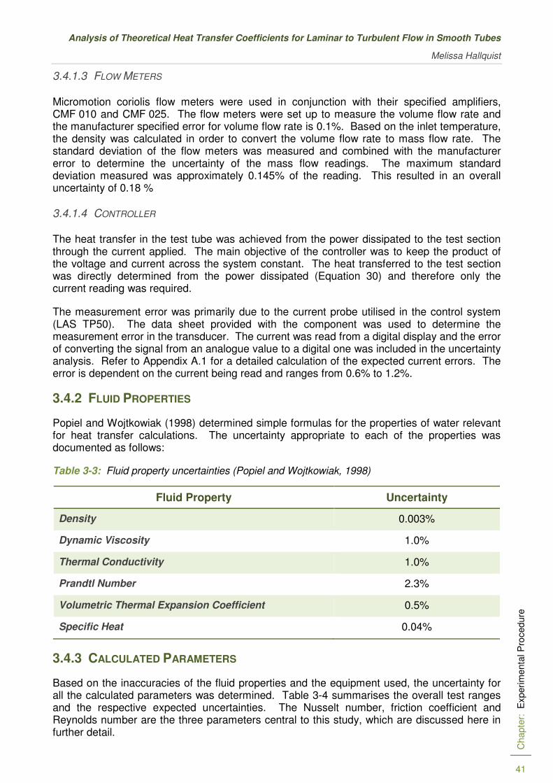
Analysis of Theoretical Heat Transfer Coefficients for Laminar to Turbulent Flow in Smooth Tubes
Melissa Hallquist
Chapte
r:
Experi
menta
l P
rocedure
41
3.4.1.3 FLOW METERS
Micromotion coriolis flow meters were used in conjunction with their specified amplifiers, CMF 010 and CMF 025. The flow meters were set up to measure the volume flow rate and the manufacturer specified error for volume flow rate is 0.1%. Based on the inlet temperature, the density was calculated in order to convert the volume flow rate to mass flow rate. The standard deviation of the flow meters was measured and combined with the manufacturer error to determine the uncertainty of the mass flow readings. The maximum standard deviation measured was approximately 0.145% of the reading. This resulted in an overall uncertainty of 0.18 %
3.4.1.4 CONTROLLER
The heat transfer in the test tube was achieved from the power dissipated to the test section through the current applied. The main objective of the controller was to keep the product of the voltage and current across the system constant. The heat transferred to the test section was directly determined from the power dissipated (Equation 30) and therefore only the current reading was required.
The measurement error was primarily due to the current probe utilised in the control system (LAS TP50). The data sheet provided with the component was used to determine the measurement error in the transducer. The current was read from a digital display and the error of converting the signal from an analogue value to a digital one was included in the uncertainty analysis. Refer to Appendix A.1 for a detailed calculation of the expected current errors. The error is dependent on the current being read and ranges from 0.6% to 1.2%.
3.4.2 FLUID PROPERTIES
Popiel and Wojtkowiak (1998) determined simple formulas for the properties of water relevant for heat transfer calculations. The uncertainty appropriate to each of the properties was documented as follows:
Table 3-3: Fluid property uncertainties (Popiel and Wojtkowiak, 1998)
Fluid Property Uncertainty
Density 0.003%
Dynamic Viscosity 1.0%
Thermal Conductivity 1.0%
Prandtl Number 2.3%
Volumetric Thermal Expansion Coefficient 0.5%
Specific Heat 0.04%
3.4.3 CALCULATED PARAMETERS
Based on the inaccuracies of the fluid properties and the equipment used, the uncertainty for all the calculated parameters was determined. Table 3-4 summarises the overall test ranges and the respective expected uncertainties. The Nusselt number, friction coefficient and Reynolds number are the three parameters central to this study, which are discussed here in further detail.

University of Pretoria
Department of Mechanical and Aeronautical Engineering
Chapte
r:
Experi
menta
l P
rocedure
42
The uncertainty of the Reynolds number is directly dependent on the accuracy of the flow meters. In each test case, the standard deviation of the flow meter is determined and combined with the specified manufactured accuracy. The average uncertainty of the Reynolds number for the CMF 010 flow meter was 0.015% (maximum uncertainty of 1.016%) and 1.02% for the CMF 025 flow meter (maximum of 1.022%). This error remains constant across the flow range measured.
Table 3-4: Overall uncertainties for all of the test cases combined
Parameter Units Range Re = 500
Q = 160W
Re = 9 250
Q = 788 W
Mass Flow Rate 0.00254-0.05627 kg/s 0.095% 0.16%
Reynolds Number Re 450-10300 1.015% 1.02%
Inlet Temperature Ti 17.9-22 °C 0.05°C 0.05°C
Change In Temperature To-Ti 32.5-1.4 °C 0.07°C 0.07°C
Heat Transfer Rate Q 160.1-788.3 W 0.06% 0.26%
Power Input elec
.
Q 160-807 W 0.88% 1.84%
Nusselt Number Nu 5.99-66.6 1.05% 1.12%
Heat Transfer Coefficient h 456-5014 W/m2K 0.30% 0.51%
Station Fluid Temperature Tf 19.8-40.4 °C 0.88% 1.85%
Friction Factor f 0.418-0.0278 0.57% 0.28%
The Nusselt number is the non-dimensional form of the heat transfer coefficient and is therefore dependent on the temperature difference between inlet and outlet, the temperature difference between the wall and the fluid, as well as the various fluid properties required in determining the Nusselt number.
The range of uncertainty of the Nusselt numbers shown in Figure 3-9 is from just over 1% in each test case to a maximum ranging from 1.06 to 1.12% increasing with decreasing heat flux.
In each of the test cases, the uncertainty of the Nusselt number increases for increasing Reynolds number. This overall increase is due to the fact that as the flow rate increases, the temperature difference between inlet and outlet decreases. The accuracy of a temperature difference reading is 0.07°C (Table 3-4) and therefore as the temperature differential decreases, the percentage error increases.
The same can be said for the difference between the wall and fluid temperatures at higher Reynolds numbers. As the flow rate increases, there is less time for heat transfer to take place resulting in a small increase in wall temperature with very little heat transfer to the fluid.
The lower the heat flux, the higher the uncertainties, with the highest uncertainty seen for the 1 451 W/m2 case. The temperature difference between inlet and outlet is directly dependent on the heat transfer achieved in the system. The higher the heat input, the higher the expected temperature differential and consequently, the lower the uncertainties expected.

Analysis of Theoretical Heat Transfer Coefficients for Laminar to Turbulent Flow in Smooth Tubes
Melissa Hallquist
Chapte
r:
Experi
menta
l P
rocedure
43
Figure 3-9: Expected uncertainties of the average Nusselt number in the 10 mm tube at different heat fluxes
The fluid properties also play a significant role in the uncertainty of the Nusselt number as shown in Table 3-3. The two properties affecting the Nusselt number is the specific heat, used to determine the heat transfer, and the thermal conductivity present when calculating the Nusselt number. The thermal conductivity ranges from 0.63 to 0.6 across the test range with an accuracy of 1% contributing to a relatively constant error. The specific heat increases with increasing Reynolds number (4 178 – 4 182) resulting in a slight increase in the uncertainty contributed to the Nusselt number. This uncertainty is relatively low and does not significantly increase the expected uncertainties.
Unlike the average Nusselt number, the local Nusselt number is based on the electric power delivered to the system. The local fluid temperatures are determined from the local power at each station, which is based on the current delivered to the system and the local resistance. The accuracy of the current is a function of the measurement and for the 10 mm tube test case, the maximum uncertainty increases from 0.6% to 1.28% over the different heat flux cases.
The error induced by the current measurement is evident in both the power delivered to the system as well as the local fluid temperature calculated, making it the driving force of the uncertainties experienced.
The local Nusselt number uncertainties are shown in Figure 3-10 showing an average uncertainty of 1.4% for the 1 451 W/m2 case, 1.6% for a heat flux of 3 225 W/m2, 1.85% for the 4 703 W/m2 case and 2.1% for the highest heat flux case. This increase in error results from the increase in error of the current measured.
In each heat flux case, the current increases slightly to maintain a constant heat flux boundary resulting in a slight increase in the uncertainties (approximately 0.02%).
1
1.02
1.04
1.06
1.08
1.1
1.12
1.14
1.16
0 1000 2000 3000 4000 5000 6000 7000 8000 9000 10000
Av
era
ge N
usselt
Nu
mb
er
Un
cert
ain
ty [
%]
Reynolds Number, Re
1 451 W/m
3 225 W/m
4 703 W/m
6 505 W/m
1 451 W/m 2
3 225 W/m 2
4 703 W/m 2
6 505 W/m 2
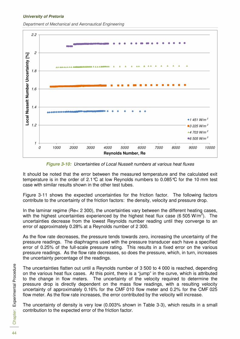
University of Pretoria
Department of Mechanical and Aeronautical Engineering
Chapte
r:
Experi
menta
l P
rocedure
44
Figure 3-10: Uncertainties of Local Nusselt numbers at various heat fluxes
It should be noted that the error between the measured temperature and the calculated exit temperature is in the order of 2.1°C at low Reynolds numbers to 0.085°C for the 10 mm test case with similar results shown in the other test tubes.
Figure 3-11 shows the expected uncertainties for the friction factor. The following factors contribute to the uncertainty of the friction factors: the density, velocity and pressure drop.
In the laminar regime (Re< 2 300), the uncertainties vary between the different heating cases, with the highest uncertainties experienced by the highest heat flux case (6 505 W/m2). The uncertainties decrease from the lowest Reynolds number reading until they converge to an error of approximately 0.28% at a Reynolds number of 2 300.
As the flow rate decreases, the pressure tends towards zero, increasing the uncertainty of the pressure readings. The diaphragms used with the pressure transducer each have a specified error of 0.25% of the full-scale pressure rating. This results in a fixed error on the various pressure readings. As the flow rate decreases, so does the pressure, which, in turn, increases the uncertainty percentage of the readings.
The uncertainties flatten out until a Reynolds number of 3 500 to 4 000 is reached, depending on the various heat flux cases. At this point, there is a “jump” in the curve, which is attributed to the change in flow meters. The uncertainty of the velocity required to determine the pressure drop is directly dependent on the mass flow readings, with a resulting velocity uncertainty of approximately 0.16% for the CMF 010 flow meter and 0.2% for the CMF 025 flow meter. As the flow rate increases, the error contributed by the velocity will increase.
The uncertainty of density is very low (0.003% shown in Table 3-3), which results in a small contribution to the expected error of the friction factor.
1
1.2
1.4
1.6
1.8
2
2.2
0 1000 2000 3000 4000 5000 6000 7000 8000 9000 10000
Lo
cal N
usselt
Nu
mb
er
Un
cert
ain
ty [
%]
Reynolds Number, Re
1 451 W/m
3 225 W/m
4 703 W/m
5 346 W/m
1 451 W/m 2
3 225 W/m 2
4 703 W/m 2
6 505 W/m 2

Analysis of Theoretical Heat Transfer Coefficients for Laminar to Turbulent Flow in Smooth Tubes
Melissa Hallquist
Chapte
r:
Experi
menta
l P
rocedure
45
The uncertainties of the 6 mm and 8 mm test sections followed the same trend and the graphs are given in Appendices A.2 and A.3 for reference.
Figure 3-11: Expected uncertainties of friction factor in the 10 mm tube at different heat fluxes
3.5 SYSTEM VALIDATION
The validation of the methodologies of determining the friction factors and heat transfer coefficients was done on a test section by taking pressure drop, voltage drop, current and temperature measurements over a wide range of mass flow rates covering the laminar, transition and turbulent flow regimes. The tube selected for validation experiments was the 6 mm tube with firstly, no heat flux (for the verification of the adiabatic pressure drop results), and secondly, with a heat flux of 3 225 W/m2. The friction factors, Nusselt numbers and Stanton numbers were then determined by using the data reduction techniques already discussed in this chapter.
The validation strategy was to compare the measurements with the work of others in the laminar and then in the turbulent flow regimes. If they compare well, then it would be a reasonable assumption to make that the measurements of this study that concentrates on the transitional flow regime (which is between the laminar and turbulent flow regime) should also be correct.
In each case, the results are compared by calculating the root mean square (RMS) error between the measured results and the predicted results. The RMS error is determined as follows:
0.2
0.22
0.24
0.26
0.28
0.3
0.32
0.34
0 1000 2000 3000 4000 5000 6000 7000 8000 9000 10000
Fri
cti
on
Facto
r U
ncert
ain
ty [
%]
Reynolds Number, Re
1 451 W/m
3 225 W/m
4 703 W/m
6 505 W/m
1 451 W/m 2
3 225 W/m 2
4 703 W/m 2
6 505 W/m 2

University of Pretoria
Department of Mechanical and Aeronautical Engineering
Chapte
r:
Experi
menta
l P
rocedure
46
( ) ( )2
22
edictedPrMeasured
RMS
σσσ
+= (50)
In the sections that follow, the adiabatic friction factors, diabatic friction factors, average Nusselt numbers, local Nusselt numbers and Stanton numbers are compared with the literature.
3.5.1 ADIABATIC FRICTION FACTORS
In Figure 3-12, the adiabatic results are shown. The results are compared with a part of the Moody chart, which is the Poiseuille equation (f = 64/Re), in the laminar flow regime; and in the turbulent flow regime, it is compared with the Blasius equation. These two equations were chosen for comparison purposes as Olivier and Meyer (2010) recently showed that their 404 measurements were within 1.5% of the Poiseuille equation and within 0.7% of the Blasius equation.
It should be noted that the friction factor results are plotted on a linear scale as opposed to the logarithmic scales traditionally used by other authors such as Cengel (2006), and Olivier and Meyer (2010). The Reynolds number range is not large enough to warrant a logarithmic scale in order to fit the data onto a reasonably sized figure (unlike the Moody chart). In addition to this, trends are clearly demonstrated on linear scales and are easier to compare.
Figure 3-12: Adiabatic friction factor for the 6 mm tube
The results in Figure 3-12, show a good agreement in the laminar flow regime (Re < 2 300) with the Poiseuille equation with an average RMS error of 1.87% and a maximum error of 9%.
0
0.02
0.04
0.06
0.08
0.1
0.12
0.14
0.16
0 2000 4000 6000 8000 10000 12000
Fri
cti
on
Facto
r, f
Reynolds Number, Re
Poiseulle
Blasius
Measurements

Analysis of Theoretical Heat Transfer Coefficients for Laminar to Turbulent Flow in Smooth Tubes
Melissa Hallquist
Chapte
r:
Experi
menta
l P
rocedure
47
Some of the results (Re < 1 000) overpredicts the friction factors while the rest of the data in the laminar region underpredicts the friction factors.
The transition point (shown as a dotted line in Figure 3-12 is at a Reynolds number of approximately 2 250, whereafter there is a sharp increase in the friction factors before the friction factors start decreasing at a Reynolds number of approximately 2 800. The transition point measured compared very well with that generally cited in literature, which is 2 300 (ASHRAE 2009) and with what was recently measured by Olivier and Meyer (2010) for fully developed flow, who have found that the transition from laminar to turbulent flow started at a Reynolds number of approximately 2 100 and ended at approximately 2 800.
In the turbulent flow regime, all the measurements were lower than those predicted by the Blasius equation. After transition, the measurements slowly converge to the Blasius equation until a Reynolds number of approximately 4 000. From this point onwards, until a Reynolds number of 11 000, the measurements underpredicted the Blasius equation with approximately 2.4%.
3.5.2 DIABATIC FRICTION FACTORS
Once the system was validated adiabatically, diabatic pressure readings were taken and the resulting friction factors compared with theoretical correlations. The diabatic friction factors are in many cases different from the adiabatic friction factors and that is why they are verified separately. This is due to the heating applied to the tube wall surface, which results in a higher wall temperature (and thus a lower viscosity) when compared with the fluid temperature at the core of the tube. This gradient is proportional to the heat applied to the test tube.
Due to this higher temperature and lower density of the fluid near the wall on the underside of the tube, the flow in a horizontal tube will circulate upward, while the fluid near the centre region of the tube, having a lower temperature and a higher density, circulates downward. These counter-rotating transverse vortices (called secondary flow) are superimposed on the primary flow due to the buoyancy forces and can significantly increase the forced convection heat transfer (Ghajar & Tam 1995) and pressure drop.
In Figure 3-13, the diabatic friction factors are compared in the laminar flow regime, with the correlation of Tam and Ghajar (1992); and in the turbulent flow regime, with the equation suggested by Allen and Eckert (1964).
The diabatic friction factors show a similar trend to the adiabatic results. For Reynolds numbers lower than 1 000, the results overpredict the friction factors (by an average of 4.5%), which would be determined using the correlation by Tam and Ghajar (1992). For Reynolds numbers between 1 000 and 2 300, the measurements underpredict the expected results by an average error of 0.6%. The profile is very similar to that predicted with an average RMS error of 2% and a maximum error of 7.1%
The transition point for the diabatic friction factor (shown as a dotted line in Figure 3-13) is at a Reynolds number of approximately 2 150. At the start of transition, the friction factors increase suddenly with a gradual transition to turbulent flow at a Reynolds number of roughly 2 600.
After transition, the measurements slowly converge to the profile predicted by Allen and Eckert (1964), however, the results consistently underpredict the expected values by approximately 1.89%. There is a slight discontinuity at a Reynolds number of 3 200, which is attributed to a change in diaphragm.

University of Pretoria
Department of Mechanical and Aeronautical Engineering
Chapte
r:
Experi
menta
l P
rocedure
48
Figure 3-13: Diabatic friction factor for the 6 mm tube at a heat flux of 2 832 W/m2
3.5.3 AVERAGE NUSSELT NUMBER
The Nusselt number was compared with two correlations: the Ghajar and Tam (1994) correlation (for laminar and turbulent flow) and the Gnielinski (1976) equation (with laminar flow being constant at 4.636).
The results of the test case are shown in Figure 3-14 indicating a smooth transition from laminar to turbulent flow. The laminar results are shown more clearly in Figure 3-15, from where it follows that the Nusselt number does not remain constant in the laminar regime. This is also shown by the results using the Ghajar and Tam correlation; however, the measured results are consistently higher (ranging from 0.3 at a Reynolds number of 1 050 to 0.66 at a Reynolds number of 2 000). The lower the heat flux, the closer the results resemble those predicted by Ghajar and Tam, which will be shown in the following chapter.
Transition from laminar to turbulent flow occurs between Reynolds numbers of 2 150 and 2 600, which corresponds to the transition measured with the pressure drops. This transition is quite steep but does follow a smooth profile.
The turbulent results resemble those predicted by Gnielinski up until a Reynolds number of approximately 3 300. The average difference between the predicted values and measured values is approximately 1.05%. At a higher Reynolds number, the results converge towards the Ghajar and Tam predictions. The scattering evident at the higher Reynolds number range is attributed to the higher uncertainties experienced at higher flow rates. The close correspondence of the results proves the validity of the test set-up.
0
0.02
0.04
0.06
0.08
0.1
0.12
0 1000 2000 3000 4000 5000 6000 7000
Fri
cti
on
Facto
r, f
Reynolds Number, Re
Measurements
Ghajar and Tam (1994)
Allen and Eckert (1964)
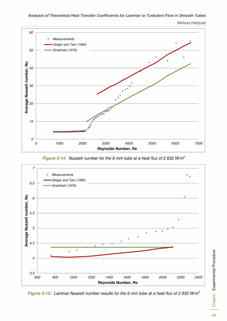
Analysis of Theoretical Heat Transfer Coefficients for Laminar to Turbulent Flow in Smooth Tubes
Melissa Hallquist
Chapte
r:
Experi
menta
l P
rocedure
49
Figure 3-14: Nusselt number for the 6 mm tube at a heat flux of 2 832 W/m2
Figure 3-15: Laminar Nusselt number results for the 6 mm tube at a heat flux of 2 832 W/m2
0
10
20
30
40
50
60
0 1000 2000 3000 4000 5000 6000 7000
Av
era
ge N
usselt
nu
mb
er,
Nu
Reynolds Number, Re
Measurements
Ghajar and Tam (1994)
Gnielinski (1976)
3.5
4
4.5
5
5.5
6
6.5
7
600 800 1000 1200 1400 1600 1800 2000 2200 2400
Av
era
ge N
usselt
nu
mb
er,
Nu
Reynolds Number, Re
Measurements
Ghajar and Tam (1994)
Gnielinski (1976)
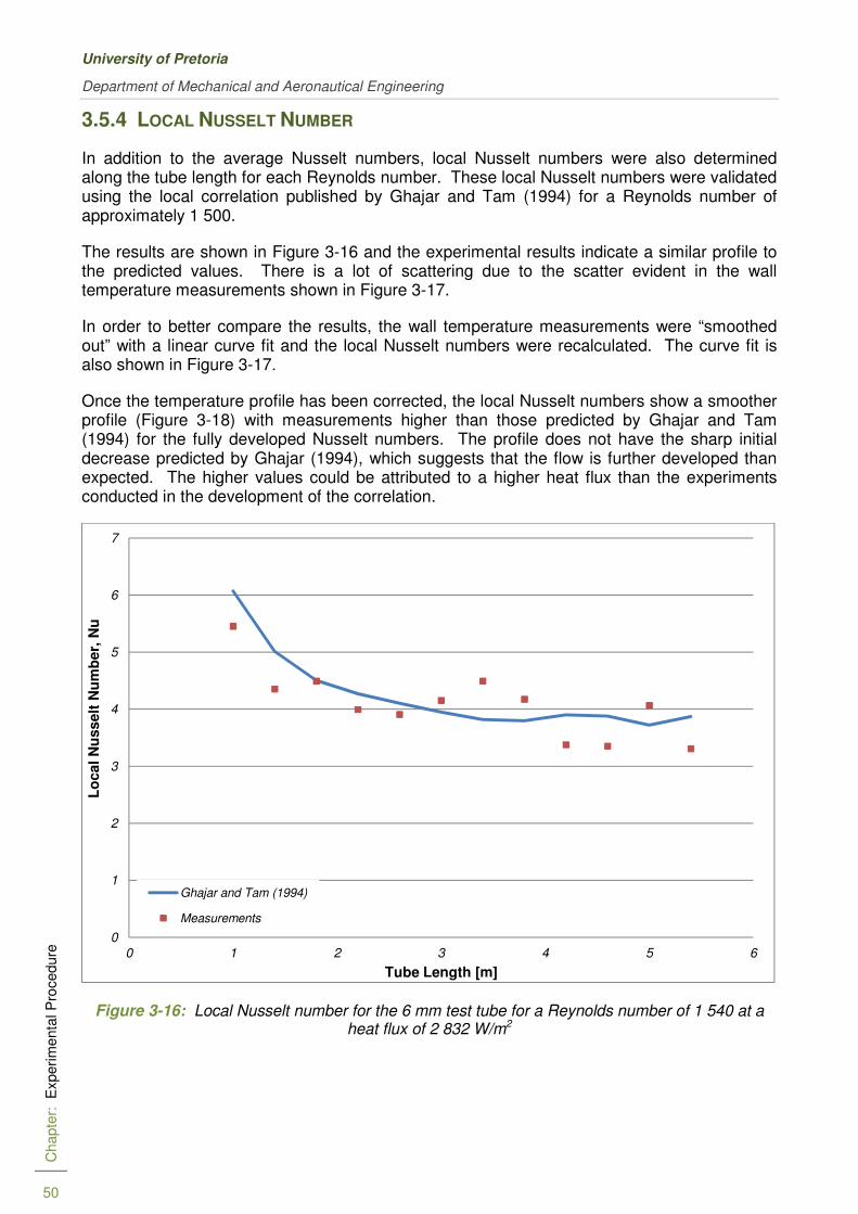
University of Pretoria
Department of Mechanical and Aeronautical Engineering
Chapte
r:
Experi
menta
l P
rocedure
50
3.5.4 LOCAL NUSSELT NUMBER
In addition to the average Nusselt numbers, local Nusselt numbers were also determined along the tube length for each Reynolds number. These local Nusselt numbers were validated using the local correlation published by Ghajar and Tam (1994) for a Reynolds number of approximately 1 500.
The results are shown in Figure 3-16 and the experimental results indicate a similar profile to the predicted values. There is a lot of scattering due to the scatter evident in the wall temperature measurements shown in Figure 3-17.
In order to better compare the results, the wall temperature measurements were “smoothed out” with a linear curve fit and the local Nusselt numbers were recalculated. The curve fit is also shown in Figure 3-17.
Once the temperature profile has been corrected, the local Nusselt numbers show a smoother profile (Figure 3-18) with measurements higher than those predicted by Ghajar and Tam (1994) for the fully developed Nusselt numbers. The profile does not have the sharp initial decrease predicted by Ghajar (1994), which suggests that the flow is further developed than expected. The higher values could be attributed to a higher heat flux than the experiments conducted in the development of the correlation.
Figure 3-16: Local Nusselt number for the 6 mm test tube for a Reynolds number of 1 540 at a heat flux of 2 832 W/m2
0
1
2
3
4
5
6
7
0 1 2 3 4 5 6
Lo
cal N
usselt
Nu
mb
er,
Nu
Tube Length [m]
Ghajar and Tam (1994)
Measurements

Analysis of Theoretical Heat Transfer Coefficients for Laminar to Turbulent Flow in Smooth Tubes
Melissa Hallquist
Chapte
r:
Experi
menta
l P
rocedure
51
Figure 3-17: Temperature distribution for the 6 mm tube for a Reynolds number of 1 540 at a heat flux of 2 832 W/m2
Figure 3-18: Local Nusselt number for the 6 mm tube for a Reynolds number of 1 540 at a heat flux of 2 832 W/m2after correcting the wall temperature
y = 2.2911x + 22.916
R² = 0.9847
0
5
10
15
20
25
30
35
40
0 1 2 3 4 5 6
Lo
cal N
usselt
Nu
mb
er,
Nu
Tube Length [m]
Wall Temperature
Fluid Temperature
Bulk Fluid Temperature
0
1
2
3
4
5
6
7
0 1 2 3 4 5 6
Lo
cal N
usselt
Nu
mb
er,
Nu
Tube Length [m]
Ghajar and Tam (1994)
Measurements
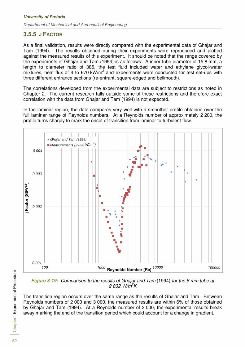
University of Pretoria
Department of Mechanical and Aeronautical Engineering
Chapte
r:
Experi
menta
l P
rocedure
52
3.5.5 J FACTOR
As a final validation, results were directly compared with the experimental data of Ghajar and Tam (1994). The results obtained during their experiments were reproduced and plotted against the measured results of this experiment. It should be noted that the range covered by the experiments of Ghajar and Tam (1994) is as follows: A inner-tube diameter of 15.8 mm, a length to diameter ratio of 385, the test fluid included water and ethylene glycol-water mixtures, heat flux of 4 to 670 kW/m2 and experiments were conducted for test set-ups with three different entrance sections (re-entrant, square-edged and bellmouth).
The correlations developed from the experimental data are subject to restrictions as noted in Chapter 2. The current research falls outside some of these restrictions and therefore exact correlation with the data from Ghajar and Tam (1994) is not expected.
In the laminar region, the data compares very well with a smoother profile obtained over the full laminar range of Reynolds numbers. At a Reynolds number of approximately 2 200, the profile turns sharply to mark the onset of transition from laminar to turbulent flow.
Figure 3-19: Comparison to the results of Ghajar and Tam (1994) for the 6 mm tube at 2 832 W/m2K
The transition region occurs over the same range as the results of Ghajar and Tam. Between Reynolds numbers of 2 000 and 3 000, the measured results are within 6% of those obtained by Ghajar and Tam (1994). At a Reynolds number of 3 000, the experimental results break away marking the end of the transition period which could account for a change in gradient.
0.001
100 1000 10000 100000
j F
acto
r [S
tPr0
.6]
Reynolds Number [Re]
Ghajar and Tam (1994)
Measurements (2 832 W/m)
0.002
0.003
0.004
W/m 2)

Analysis of Theoretical Heat Transfer Coefficients for Laminar to Turbulent Flow in Smooth Tubes
Melissa Hallquist
Chapte
r:
Experi
menta
l P
rocedure
53
At a Reynolds number of 4 800, Ghajar and Tam’s results start to decrease. The same happens with the experimental results, however, at this point the expected uncertainties are relatively high and scattering is evident in the results. Ghajar’s experiments extended to a Reynolds number of 49 000, which was not possible in the present study.
It should be noted that the results obtained in these experiments were for different flow ranges: the Prandtl number ranged from 4 to 158 with a test heat flux of 4 to 670 kW/m2. These different test conditions account for the differences between the measurements and the work of Ghajar and Tam.
Similar validations were done for the other tube diameters at different heat flux conditions. In general, the tendencies were the same and it could therefore be concluded that the experimental methodology, data captivity and data reduction processes were correct due to the good results obtained. This gave good confidence that the results generated and discussed in the following chapter are correct.
3.5.6 SUMMARY
This chapter discussed the experimental set-up and procedure followed in obtaining the results presented in the following chapter. The test set-up consisted of an overall system supplying water to a removable test section with a direct current welder that heats the fluid flowing through the test section. There were three types of Nusselt numbers to be considered in this study, namely the local, average and fully developed Nusselt numbers, which were discussed in the data reduction.
The expected errors of the measurements were determined based on the uncertainties of the equipment and the properties that were calculated. These errors were considered to be within reasonable limits as was shown by the system validation. Comparisons were made between the measured results and those obtained by Ghajar and Tam (1994) as well as by Allen and Eckert (1964) for the diabatic friction factor.
The Nusselt number was compared with the results of Ghajar and Tam (1994) as well as Gnielinski (1976) and finally the Stanton number was compared with the experimental results of Ghajar and Tam (1994). In general, good agreement was found and it can be concluded that the experimental set-up generated accurate measurements of the heat transfer coefficient and friction factors in the transitional regime.


Analysis of Theoretical Heat Transfer Coefficients for Laminar to Turbulent Flow in Smooth Tubes
Melissa Hallquist
Chapte
r: R
esults
55
4. RESULTS
4.1 INTRODUCTION
Once the test set-up was validated, results were captured for all three tube sizes at different heat fluxes concentrating on the transition region. The results are first described for the diabatic friction factors recorded and then the heat transfer aspects are discussed.
4.2 DIABATIC FRICTION FACTORS
For each test section, the friction factors were recorded for four different heat fluxes. The results for the 10 mm tube are given in Figure 4-1.
For each heat flux case, the friction factors in the laminar flow region follow the same trend. For the higher heat flux cases, outlet temperatures would be high enough to result in boiling of the water near the outlet and therefore the lowest Reynolds number considered is approximately 1 600 and in these cases, comparison of results is limited to the lower heat flux cases.
At Reynolds numbers below 1 000, a trend is seen where the higher the heat input to the system, the higher the friction factor. This trend is inversed as the flow approaches transition to turbulent flow. A close-up of the transition region is shown in Figure 4-1b. The higher the heat flux, the higher the temperature difference between the wall and the core fluid. This results in a higher viscosity ratio for increased heat flux and therefore an increase in the friction factor. As the flow rate increases, secondary flow effects become less prominent, which could account for the inverse at the onset of transition.
In each of the heat flux cases, transition from laminar to turbulent flow is a smooth process with the onset of transition being delayed with an increase in heat flux. For a heat flux of 1 451 W/m2, the onset of transition is at a Reynolds number of 2 040. When the heat flux is increased 3 225 W/m2, transition occurs at a Reynolds number of approximately 2 140. Transition is further delayed with higher heat fluxes with onset at 2 230 and 2 340 for a heat flux of 4 703 W/m2 and 6 505 W/m2 respectively.
Once transition is achieved, the friction factors increase along the same gradient for each case and transitional flow occurs over the same size Reynolds range meaning that the end of transition is also delayed with increased heat flux. Note that the higher the heat flux, the lower the friction factors over the transition regime. This is because of the decrease of the viscosity on the tube wall with an increase in temperature.
Once turbulent flow has been established, the friction factors of the different heat flux cases tend to converge. At a Reynolds number of approximately 4 700, the average deviation of the friction factors for each heating case is 1.4% with a maximum deviation of 2.7%.
The results of the 6 mm and 8 mm tubes are included in this section to determine whether the same trends were evident in all the test cases. Figure 4-2 shows the results for the full Reynolds number range of the 6 mm tube.
Once again there is a trend at the bottom end of the laminar flow range where the friction factors increase for a decreasing heat input. In this case, the inverse of this trend is also evident at a Reynolds number of approximately 1 600 where the 6 505 W/m2 heat flux exhibits the lowest friction factor.

University of Pretoria
Department of Mechanical and Aeronautical Engineering
Chapte
r: R
esults
56
Figure 4-1: Average diabatic friction factors for different heat fluxes for the 10 mm tube: (a) full Reynolds number range, (b) transition region
0
0.02
0.04
0.06
0.08
0.1
0.12
0.14
0.16
0.18
0.2
0 1000 2000 3000 4000 5000 6000 7000 8000 9000 10000
Fri
cti
on
Facto
r, f
Reynolds Number, Re
1 451 W/m
3 225 W/m
4 703 W/m
6 505 W/m
0.02
0.025
0.03
0.035
0.04
0.045
0.05
1800 2000 2200 2400 2600 2800 3000 3200
Fri
cti
on
Facto
r, f
Reynolds Number, Re
1 451 W/m
3 225 W/m
4 703 W/m
6 505 W/m
1 451 W/m 2
3 225 W/m 2
4 703 W/m 2
6 505 W/m 2
1 451 W/m 2
3 225 W/m 2
4 703 W/m 2
6 505 W/m 2
(a)
(b)
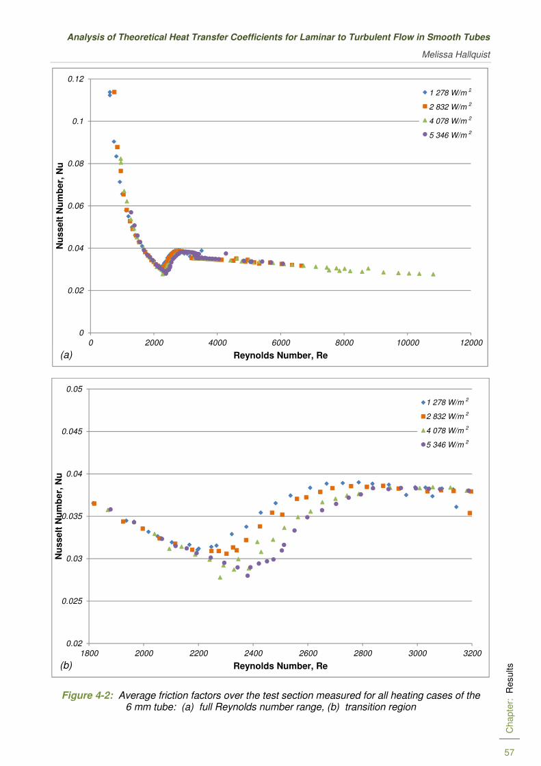
Analysis of Theoretical Heat Transfer Coefficients for Laminar to Turbulent Flow in Smooth Tubes
Melissa Hallquist
Chapte
r: R
esults
57
Figure 4-2: Average friction factors over the test section measured for all heating cases of the 6 mm tube: (a) full Reynolds number range, (b) transition region
0
0.02
0.04
0.06
0.08
0.1
0.12
0 2000 4000 6000 8000 10000 12000
Nu
sselt
Nu
mb
er,
Nu
Reynolds Number, Re
1 278 W/m
2 832 W/m
4 078 W/m
5 346 W/m
0.02
0.025
0.03
0.035
0.04
0.045
0.05
1800 2000 2200 2400 2600 2800 3000 3200
Nu
sselt
Nu
mb
er,
Nu
Reynolds Number, Re
1 278 W/m
2 832 W/m
4 078 W/m
5 346 W/m
1 278 W/m 2
2 832 W/m 2
4 078 W/m 2
5 346 W/m 2
1 278 W/m 2
2 832 W/m 2
4 078 W/m 2
5 346 W/m 2
(a)
(b)
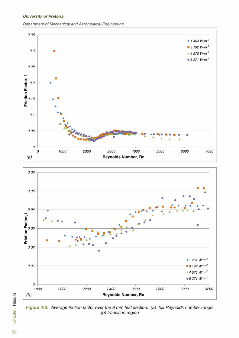
University of Pretoria
Department of Mechanical and Aeronautical Engineering
Chapte
r: R
esults
58
Figure 4-3: Average friction factor over the 8 mm test section: (a) full Reynolds number range, (b) transition region
0
0.05
0.1
0.15
0.2
0.25
0.3
0.35
0 1000 2000 3000 4000 5000 6000 7000
Fri
cti
on
Facto
r, f
Reynolds Number, Re
1 464 W/m
3 192 W/m
4 575 W/m
6 271 W/m
0
0.01
0.02
0.03
0.04
0.05
0.06
1800 2000 2200 2400 2600 2800 3000 3200
Fri
cti
on
Facto
r, f
Reynolds Number, Re
1 464 W/m
3 192 W/m
4 575 W/m
6 271 W/m
1 464 W/m 2
3 192 W/m 2
4 575 W/m 2
6 271 W/m 2
1 464 W/m 2
3 192 W/m 2
4 575 W/m 2
6 271 W/m 2
(a)
(b)

Analysis of Theoretical Heat Transfer Coefficients for Laminar to Turbulent Flow in Smooth Tubes
Melissa Hallquist
Chapte
r: R
esults
59
The onset of transition is again dependent on the amount of heat input into the system. For the 1 278 W/m2 case, the onset of transition occurs at a Reynolds number of 2 050. At a heat flux of 2 832 W/m2, transition starts at a Reynolds number of 2 180. The onset of transition for the higher heat flux cases is at a Reynolds number of 2 240 and 2 300 at heat flux of 4 078 W/m2 and 5 346 W/m2 respectively.
In this case, the results converge at a Reynolds number of approximately 3 000, which marks the end of the transition region. The friction factor decreases from approximately 0.0385 at a Reynolds number of 3 000 to 0.028 at a Reynolds number of 11 300.
The results of the 8 mm tube are shown in Figure 4-3. The results of the 8 mm tube are not as smooth as those of the other two test sections. Transition is also dependent on the heat flux of the system with transition occurring at a Reynolds number of 2 080 and 2 300 for a heat flux of 1 464 W/m2 and 3 192 W/m2 respectively. For a heat flux of 4 575 W/m2, the onset of transition occurs at a Reynolds number of 2 400 and in the highest heat flux case, transition starts at a Reynolds number of 2 420.
At a Reynolds number of 2 800, the friction factor of the 6 271 W/m2 heat flux case overshoots the expected values before converging with the remainder of results at a Reynolds number of 3 300. At a Reynolds number of 4 000, the friction factor for the 4 575 W/m2 case breaks away from the other results, with the friction factor decreasing from 0.04 to 0.02.
Figure 4-4: Comparison of friction factor across the different tube sizes
The 3 000 W/m2 heat flux case for each of the three test sections is plotted in Figure 4-4. The results of the 6 mm and 10 mm tube are very close to one another with the 6 mm results measuring approximately 1.3% higher than the 10 mm results in the early laminar flow regime. As the flow starts to approach transition, this difference increases to approximately 4.7% at a Reynolds number of 2 030. After transition, the results start to converge at a Reynolds
0
0.05
0.1
0.15
0.2
0.25
0.3
0.35
0 1000 2000 3000 4000 5000 6000 7000 8000 9000
Fri
cti
on
Facto
r, f
Reynolds Number, Re
6 mm Tube
8 mm Tube
10 mm Tube

University of Pretoria
Department of Mechanical and Aeronautical Engineering
Chapte
r: R
esults
60
number of approximately 3 200 after which the 6 mm results start to measure lower friction factors than the 10 mm results.
The results of the 8 mm tube do not conform as well to the other two test cases. The decrease in friction factor over the laminar regime is more severe in this case. Over the transitional regime, the results do converge with the results lying between the 6 mm and 10 mm test cases at a Reynolds number of around 2 400. At the onset of transition, there is a “step” in the 8 mm results which could be due to an incorrect overlap between diaphragms during the measurements.
Based on the above results, it can be concluded that transition from laminar to turbulent flow is a smooth process with no discontinuities evident in the measured results. In the laminar regime, the friction factors are higher for higher heat flux cases and transition is delayed by increasing the heat flux of the system. Once turbulent flow is achieved, the different heat flux results tend to converge suggesting that the viscosity ratio no longer plays a significant role.
4.3 HEAT TRANSFER
The local, average and fully developed Nusselt numbers are illustrated in this section. The Stanton number is also presented in the results to directly compare the experimental results with those of Ghajar and Tam (1994).
Before discussing the results, the Raleigh number is presented in Figure 4-5 for all the test sections in order to determine the flow regime of the results.
Mixed convection is only evident in the laminar regime for Raleigh numbers greater than 105. The only Raleigh numbers above 105 are the lowest values measured for the 6 505 W/m2 case, however, the Reynolds number in these cases is above 1 000. Based on the flow regime map these results also fall within the forced convection range.
In the turbulent regime, the heat transfer is considered to be mixed for Raleigh numbers greater than approximately 107. The Raleigh numbers of the current study are well below this boundary and it can therefore be concluded that all test results are based in the forced convection regime.
The Raleigh number increases for decreasing Reynolds number. The same trend is followed in each of the test cases. In the laminar regime, there is a steep decrease in the Raleigh number with increasing Reynolds numbers. The gradient changes at the onset of transition and again once the flow is completely turbulent. As the heat flux into the system is increased, the Raleigh number increases and is consistently higher than the Raleigh numbers associated with lower heat flux inputs.
In addition to the flow regime map, the Gr/Re2 parameter has been determined for all the test results. This parameter ranges from a minimum of 4.884.10-7 for the 6 mm test case to a maximum of 0.0377 for the 10 mm test section. This confirms that natural convection effects are negligible for the entire test range as Gr/Re2<0.1 (Cengel 2006). The implication of this is that variations in the friction factor and Nusselt number cannot be attributed to secondary flow but must be accounted for by changes in fluid properties.

Analysis of Theoretical Heat Transfer Coefficients for Laminar to Turbulent Flow in Smooth Tubes
Melissa Hallquist
Chapte
r: R
esults
61
Figure 4-5: Raleigh number results for all the test cases
However, this is contradicted when the local heat transfer of the top half of the test section is compared with the heat transfer of the bottom, as investigated by Ghajar and Tam (1994).
In the absence of buoyancy effects, all four thermocouples should read approximately the same temperature irrespective of thermocouple placement. Figure 4-6 gives a typical temperature profile for the 10 mm test section at the last station before mixing occurs.
At a Reynolds number of approximately 1 500, the temperature ranges from 55°C at the top of the tube to about 48°C at the bottom represented in the figure by a screwed diamond shape. As the flow rate increases, the temperature profile becomes evenly shaped indicating the absence of buoyancy effects. At the highest Reynolds number measured, the temperature at the top and bottom of the tube is 22.8°C and 22.9°C respectively (a difference of only 0.18%).
This trend is evident as early as the first measurement station with a more prominent profile developing along the length of the test section.
1.E+02
1.E+03
1.E+04
1.E+05
1.E+01 1.E+02 1.E+03 1.E+04 1.E+05 1.E+06
Reyn
old
s N
um
ber,
Re
Raleigh Number, Ra
6mm Tube - 1 278
2 832
4 078
5 346
1 464
3 192
4 575
6 271
1 451
3 225
4 703
6 505
6 mm Tube - 1 268 W/m 2
6 mm Tube - 2 832 W/m 2
6 mm Tube - 4 078 W/m 2
6 mm Tube - 5 346 W/m 2
8 mm Tube - 1 464 W/m 2
8 mm Tube - 3 192 W/m 2
8 mm Tube - 4 575 W/m 2
8 mm Tube - 6 271 W/m 2
10 mm Tube - 1 451 W/m 2
10 mm Tube - 3 225 W/m 2
10 mm Tube - 4 703 W/m 2
10 mm Tube - 6 505 W/m 2

University of Pretoria
Department of Mechanical and Aeronautical Engineering
Chapte
r: R
esults
62
Figure 4-6: Temperature profile for the 10 mm test section at a heat flux of 6 505 W/m2
Figure 4-7: Local heat transfer ratio for the 10 mm test case at a heat flux of 6 505 W/m2
-60
-40
-20
0
20
40
60
-60 -40 -20 0 20 40 60
Temperature [°C]
Re = 1 500
Re = 1 800
Re = 2 100
Re = 2 400
Re = 2 700
Re = 3 000
Re = 6 100
Re = 8 900
0
0.2
0.4
0.6
0.8
1
1.2
0 1000 2000 3000 4000 5000 6000 7000 8000 9000
Lo
cal H
eat
Tra
nsfe
r R
ati
o,
h(x
) t/h
(x) b
Reynolds number, Re
Top
Bottom
Right Left

Analysis of Theoretical Heat Transfer Coefficients for Laminar to Turbulent Flow in Smooth Tubes
Melissa Hallquist
Chapte
r: R
esults
63
The average temperature along the top of the test section was used to determine the average local heat transfer coefficient for the top half of the test section for each flow rate tested. The same was done for the bottom temperature in order to determine the local heat transfer coefficient ratio (ht/hb). Figure 4-7 gives the heat transfer coefficient ratio for varying Reynolds numbers in the 10 mm test case at a heat flux of 6 505 W/m2.
The heat transfer coefficient ratio increases with increasing Reynolds numbers. As the flow approaches transition, there is a sharp increase in the ratio, which approaches 0.8 at a Reynolds number of 2 400. This suggests that secondary flow effects decrease as the flow enters the transitional flow regime. At a Reynolds number of approximately 2 700, the ratio approaches unity, which implies no secondary flow influences.
A similar trend is seen in the other test cases where the influence of secondary flow is strongly related to the different flow regimes. From this, it is concluded that secondary flow influences the heat transfer measurements in the laminar flow regime. Once the flow enters the transitional flow regime, there is still a small influence which ends once the flow becomes turbulent.
4.3.1 LOCAL NUSSELT NUMBER
In this section, the local Nusselt numbers are presented as a function of the flow regime. A sample based on a Reynolds case for each of the three flow regimes is given for the various test cases. As discussed in Section 3.5.4, the wall temperature measurements have slight irregularities resulting in an irregular profile in the local Nusselt number. As with the results presented in Section 3.5.4, a straight line is fitted to the wall temperature measurements, which smooths out the local Nusselt number readings to aid in comparing the results.
4.3.1.1 LAMINAR FLOW
The Reynolds number case selected for the laminar flow discussion is approximately 1 850. The local Nusselt number is plotted as a function of the heat exchanger position in the form of the length over the diameter (x/d) as found in other studies (Ghajar & Tam 1994).
The results of the 6 mm test case are presented in Figure 4-8. The Nusselt number decreases along the length of the test section, where the gradient of decrease is steeper for decreasing heat flux cases.
In general, the Nusselt number is higher for increasing heat flux cases. The average Nusselt number for the 1 278 W/m2 case is approximately 3.62, which increases to 4.85 for the 2 832 W/m2 heat flux case. The average Nusselt number increases further to 5 and 5.5 in the 4 078 W/m2 and 5 346 W/m2 cases respectively. As the heat flux increases, the temperature differential between the fluid and the wall increases resulting in a higher heat transfer coefficient.
The fluid should be thermally fully developed at a position (x/d) of 500 illustrated in Figure 4-8 by the dashed red line. The local Nusselt number should flatten out once developed, which is not the case, suggesting that the flow had not fully developed in each of the test cases.
The 8 mm test case results are given in Figure 4-9 and once again the Nusselt numbers are higher for increasing heat flux cases. For the lowest heat flux case, the average Nusselt number is 6.23, which increases to 8.08 for the 3 192 W/m2 case. For the 4 575 W/m2 and 6 271 W/m2 cases, the Nusselt number is 8.68 and 9.74 respectively.

University of Pretoria
Department of Mechanical and Aeronautical Engineering
Chapte
r: R
esults
64
Figure 4-8: Local Nusselt numbers for the 6 mm test case at an average Reynolds number of approximately 1 845
When compared with the 6 mm results, the Nusselt numbers are higher in this case. The Nusselt number is a function of the tube diameter, which accounts for the increase in bigger tube sizes.
The Nusselt number only decreases along the length of the tube for the lowest heat flux case. In the other cases, the Nusselt number increases exponentially along the length of the tube, with the gradient being higher for higher heat flux cases.
The Nusselt number should be fully developed after a tube position of 547. The only results that appear to be fully developed (illustrated by a flattened-out curve) are the 1 464 W/m2 results.
The 10 mm results are given in Figure 4-10. The Nusselt number shows the same trend as the 8 mm tube. Once again the Nusselt numbers are higher than the smaller tube diameters with the average Nusselt numbers increasing as follows: 6.6 for a heat flux of 1 451 W/m2, 8.1 for 3 225 W/m2, 9.2 for 4 703 W/m2 and 10.5 for a heat flux of 6 505 W/m2.
In this case, the thermally fully developed flow is at 542 and once again only the lowest heat flux case shows a flattened profile typical of a fully developed flow.
In general, when comparing the results in Figure 4-8 with those in Figure 4-10, the Nusselt numbers increase as the tube diameters increase.
0
1
2
3
4
5
6
0 200 400 600 800 1000 1200 1400
Lo
cal N
usselt
Nu
mb
er,
Nu
Tube Position, x/d
1 278 W/m
2 832 W/m
4 078 W/m
5 346 W/m
1 278 W/m 2
2 832 W/m 2
4 078 W/m 2
5 346 W/m 2

Analysis of Theoretical Heat Transfer Coefficients for Laminar to Turbulent Flow in Smooth Tubes
Melissa Hallquist
Chapte
r: R
esults
65
Figure 4-9: Local Nusselt number at Reynolds number of 1 869 for the 8 mm test section
Figure 4-10: Local Nusselt number for the 10 mm test case at an average Reynolds number of approximately 1 843
0
2
4
6
8
10
12
14
0 100 200 300 400 500 600 700 800 900 1000
Lo
cal N
usselt
Nu
mb
er,
Nu
Tube Position, x/d
1 464 W/m
3 192 W/m
4 575 W/m
6 271 W/m
0
2
4
6
8
10
12
14
16
0 100 200 300 400 500 600 700 800
Lo
cal N
usselt
Nu
mb
er,
Nu
Tube Position, x/d
1 451 W/m
3 225 W/m
4 703 W/m
6 505 W/m
1 464 W/m 2
3 192 W/m 2
4 575 W/m 2
6 271 W/m 2
1 451 W/m 2
3 225 W/m 2
4 703 W/m 2
6 505 W/m 2

University of Pretoria
Department of Mechanical and Aeronautical Engineering
Chapte
r: R
esults
66
4.3.1.2 TURBULENT FLOW
Turbulent flow is thermally fully developed at 10d and therefore all the results should already be fully developed as the first measuring point is at x/d = 250.
The 6 mm results are shown in Figure 4-11, and as with the laminar results, the Nusselt number decreases along the length of the test tube. The test range for the 1 278 W/m2 did not extend past a Reynolds number of 3 600 and therefore is not included in the results.
Figure 4-11: Turbulent results for the local Nusselt number for the 6 mm test case at a Reynolds number of 5 355
It should be noted that the 2 832 W/m2 case is on the upper boundary of measurements and is associated with higher uncertainties.
The gradient increases with decreasing heat flux where the 5 346 W/m2 case decreases from 37.8 to 33.2, the 4 078 W/m2 decreases by 4 from 32.4 and the final case decreases by 11 down to 16.6.
The results of the 10 mm tube is given in Figure 4-12. The lowest heat flux case is the only one in which the Nusselt number does not increase along the length of the heat exchanger, which is the same trend seen in the laminar results. The flattened profile of the Nusselt number is as expected for thermally developed flow.
0
5
10
15
20
25
30
35
40
0 200 400 600 800 1000 1200 1400 1600
Lo
cal N
usselt
Nu
mb
er
Tube Position, x/d
2 832 W/m
4 078 W/m
5 346 W/m
2 832 W/m 2
4 078 W/m 2
5 346 W/m 2
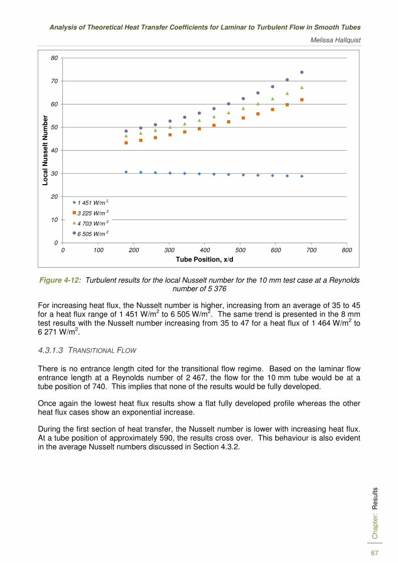
Analysis of Theoretical Heat Transfer Coefficients for Laminar to Turbulent Flow in Smooth Tubes
Melissa Hallquist
Chapte
r: R
esults
67
Figure 4-12: Turbulent results for the local Nusselt number for the 10 mm test case at a Reynolds number of 5 376
For increasing heat flux, the Nusselt number is higher, increasing from an average of 35 to 45 for a heat flux range of 1 451 W/m2 to 6 505 W/m2. The same trend is presented in the 8 mm test results with the Nusselt number increasing from 35 to 47 for a heat flux of 1 464 W/m2 to 6 271 W/m2.
4.3.1.3 TRANSITIONAL FLOW
There is no entrance length cited for the transitional flow regime. Based on the laminar flow entrance length at a Reynolds number of 2 467, the flow for the 10 mm tube would be at a tube position of 740. This implies that none of the results would be fully developed.
Once again the lowest heat flux results show a flat fully developed profile whereas the other heat flux cases show an exponential increase.
During the first section of heat transfer, the Nusselt number is lower with increasing heat flux. At a tube position of approximately 590, the results cross over. This behaviour is also evident in the average Nusselt numbers discussed in Section 4.3.2.
0
10
20
30
40
50
60
70
80
0 100 200 300 400 500 600 700 800
Lo
cal N
usselt
Nu
mb
er
Tube Position, x/d
1 451 W/m
3 225 W/m
4 703 W/m
6 505 W/m
1 451 W/m 2
3 225 W/m 2
4 703 W/m 2
6 505 W/m 2

University of Pretoria
Department of Mechanical and Aeronautical Engineering
Chapte
r: R
esults
68
Figure 4-13: Transitional local Nusselt numbers for the 10 mm test case at a Reynolds number of 2 467
4.3.1.4 SUMMARY
The following conclusions have been drawn for the local Nusselt number based on the results in Chapter 4:
Fully developed flow in the laminar flow regime is only evident in the lowest heat flux cases of the 8 mm and 10 mm test sections. This contradicts the theory that suggests that natural convection effects should be negligible for all the results obtained in this study. In addition, the 8 mm and 10 mm results show an exponential increase of the local Nusselt number along the length of the tube. The Nusselt number is higher for increased heat flux and also for larger diameter test sections.
In the turbulent flow example, the local Nusselt number decreases along the length of the tube for the 6 mm results, but not for the other two test cases. All the results should resemble a straight line characteristic of fully developed flow, which is not the case. As with the laminar results, the Nusselt number is higher for increased heat flux and tube diameters.
The transition results do not resemble either the laminar or turbulent results. In this case, the local Nusselt number is higher for decreasing heat flux (with the exception of the lowest heat flux case). The local Nusselt number once again increases exponentially along the length of the test section converging towards the end of the test section.
0
5
10
15
20
25
0 100 200 300 400 500 600 700 800
Lo
cal N
usselt
Nu
mb
er
Tube Position, x/d
1 451 W/m
3 225 W/m
4 703 W/m
6 505 W/m
1 451 W/m 2
3 225 W/m 2
4 703 W/m 2
6 505 W/m 2
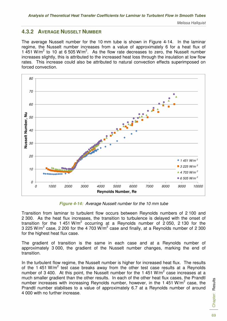
Analysis of Theoretical Heat Transfer Coefficients for Laminar to Turbulent Flow in Smooth Tubes
Melissa Hallquist
Chapte
r: R
esults
69
4.3.2 AVERAGE NUSSELT NUMBER
The average Nusselt number for the 10 mm tube is shown in Figure 4-14. In the laminar regime, the Nusselt number increases from a value of approximately 6 for a heat flux of 1 451 W/m2 to 10 at 6 505 W/m2. As the flow rate decreases to zero, the Nusselt number increases slightly, this is attributed to the increased heat loss through the insulation at low flow rates. This increase could also be attributed to natural convection effects superimposed on forced convection.
Figure 4-14: Average Nusselt number for the 10 mm tube
Transition from laminar to turbulent flow occurs between Reynolds numbers of 2 100 and 2 300. As the heat flux increases, the transition to turbulence is delayed with the onset of transition for the 1 451 W/m2 occurring at a Reynolds number of 2 050, 2 130 for the 3 225 W/m2 case, 2 200 for the 4 703 W/m2 case and finally, at a Reynolds number of 2 300 for the highest heat flux case.
The gradient of transition is the same in each case and at a Reynolds number of approximately 3 000, the gradient of the Nusselt number changes, marking the end of transition.
In the turbulent flow regime, the Nusselt number is higher for increased heat flux. The results of the 1 451 W/m2 test case breaks away from the other test case results at a Reynolds number of 3 400. At this point, the Nusselt number for the 1 451 W/m2 case increases at a much smaller gradient than the other results. In each of the other heat flux cases, the Prandtl number increases with increasing Reynolds number, however, in the 1 451 W/m2 case, the Prandtl number stabilises to a value of approximately 6.7 at a Reynolds number of around 4 000 with no further increase.
0
10
20
30
40
50
60
70
80
0 1000 2000 3000 4000 5000 6000 7000 8000 9000 10000
Nu
sselt
Nu
mb
er,
Nu
Reynolds Number, Re
1 451 W/m
3 225 W/m
4 703 W/m
6 505 W/m
1 451 W/m 2
3 225 W/m 2
4 703 W/m 2
6 505 W/m 2

University of Pretoria
Department of Mechanical and Aeronautical Engineering
Cha
pter
: 3B
Res
ults
70
The results of the 6 mm test section are shown in Figure 4-15. As with the 10 mm test case, the Nusselt number in the laminar regime increases with increasing heat flux. In this case, the Nusselt number does not increase as the flow rate approaches zero, but rather increases slowly as the flow rate approaches transition.
Figure 4-15: Average Nusselt number for the 6 mm tube
The onset of transition is delayed for increasing heat flux. Transition occurs at a Reynolds number of 2 077 for 1 278 W/m2 and is delayed to a Reynolds number of 2 300 for a heat flux of 5 346 W/m2. During transition, the Nusselt number is lower for increasing heat flux. In this case, the gradient of transition is greater for higher heat flux cases. The end of transition is marked by a change in gradient at a Reynolds number of approximately 2 600.
In the 1 278 W/m2 heat flux case, the results break away at a Reynolds number of 3 100 increasing at a much higher gradient than the rest of the results. These data points are associated with high uncertainties due to the small temperature difference between inlet and outlet.
After a Reynolds number of 3 500, the Nusselt number for the different heat fluxes increases at the same gradient. There is some scattering at these higher Reynolds numbers due to the increased uncertainties associated with higher flow rates.
The results of the 8 mm test case are given in Figure 4-16. The results in this case are not as “smooth” as the other test cases.
In the laminar regime, the Nusselt number also increases with increased heat flux, increasing from 7 for a heat flux of 1 464 W/m2 to 10 for a heat flux of 6 271 W/m2. As with the 8 mm case, the Nusselt number increases as the flow rate approaches zero flow rate. At a Reynolds number of 2 000, the Nusselt number increases slightly before the onset of transition.
0
10
20
30
40
50
60
70
0 2000 4000 6000 8000 10000 12000
Nus
selt
Num
ber,
Nu
Reynolds Number, Nu]
1 278 W/m
2 832 W/m
4 078 W/m
5 346 W/m
1 278 W/m 2
2 832 W/m 2
4 078 W/m 2
5 346 W/m 2
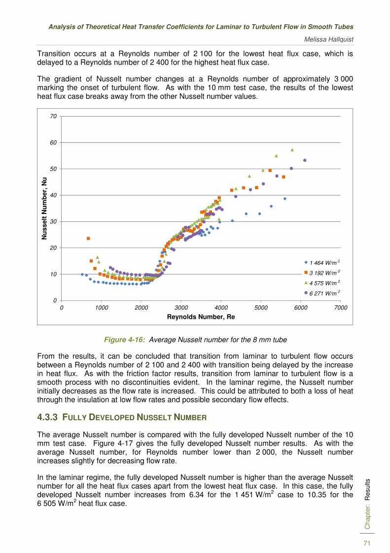
Analysis of Theoretical Heat Transfer Coefficients for Laminar to Turbulent Flow in Smooth Tubes
Melissa Hallquist
Chapte
r: R
esults
71
Transition occurs at a Reynolds number of 2 100 for the lowest heat flux case, which is delayed to a Reynolds number of 2 400 for the highest heat flux case.
The gradient of Nusselt number changes at a Reynolds number of approximately 3 000 marking the onset of turbulent flow. As with the 10 mm test case, the results of the lowest heat flux case breaks away from the other Nusselt number values.
Figure 4-16: Average Nusselt number for the 8 mm tube
From the results, it can be concluded that transition from laminar to turbulent flow occurs between a Reynolds number of 2 100 and 2 400 with transition being delayed by the increase in heat flux. As with the friction factor results, transition from laminar to turbulent flow is a smooth process with no discontinuities evident. In the laminar regime, the Nusselt number initially decreases as the flow rate is increased. This could be attributed to both a loss of heat through the insulation at low flow rates and possible secondary flow effects.
4.3.3 FULLY DEVELOPED NUSSELT NUMBER
The average Nusselt number is compared with the fully developed Nusselt number of the 10 mm test case. Figure 4-17 gives the fully developed Nusselt number results. As with the average Nusselt number, for Reynolds number lower than 2 000, the Nusselt number increases slightly for decreasing flow rate.
In the laminar regime, the fully developed Nusselt number is higher than the average Nusselt number for all the heat flux cases apart from the lowest heat flux case. In this case, the fully developed Nusselt number increases from 6.34 for the 1 451 W/m2 case to 10.35 for the 6 505 W/m2 heat flux case.
0
10
20
30
40
50
60
70
0 1000 2000 3000 4000 5000 6000 7000
Nu
sselt
Nu
mb
er,
Nu
Reynolds Number, Re
1 464 W/m
3 192 W/m
4 575 W/m
6 271 W/m
1 464 W/m 2
3 192 W/m 2
4 575 W/m 2
6 271 W/m 2

University of Pretoria
Department of Mechanical and Aeronautical Engineering
Chapte
r: R
esults
72
For the 1 451 W/m2 case at a Reynolds number of approximately 3 700, the results break away from the other heat flux cases, which was also seen with the smaller gradient observed in the average Nusselt numbers. This could be attributed to the higher uncertainties experienced in the current measurements for this test case. In the 3 225 W/m2 case, there is a slight jump in the Nusselt number at a Reynolds number of 2 600 and again at a Reynolds number of 3 600. This trend is also seen in the average Nusselt number on a much smaller scale.
Transition for each heat flux case occurs at the same Reynolds number as with the average Nusselt numbers. The Nusselt numbers in the turbulent regime are higher than the average Nusselt numbers.
Figure 4-17: Fully developed Nusselt number for the 10 mm tube
4.3.4 THE J FACTOR
Figure 4-18 gives the j factor appropriate to all the heat flux cases of the 10 mm test tube on a log-log scale. For comparison, the results of the 6 mm and 8 mm tubes are given in Figure 4-19 and Figure 4-20 respectively.
In each of the cases, the same trend is seen in the laminar flow regimes. The j factor is higher for higher heat flux inputs with the same gradient in each of the heat fluxes. A sharp change in gradient marks the onset of transition, and as with the Nusselt number results, the onset of transition is delayed with increasing heat flux.
0
10
20
30
40
50
60
0 1000 2000 3000 4000 5000 6000 7000 8000 9000 10000
Fu
lly D
ev
elo
ped
Nu
sselt
Nu
mb
er,
Nu
fd
Reynolds Number, Re
1 451 W/m
3 225 W/m
4 703 W/m
6 505 W/m
1 451 W/m 2
3 225 W/m 2
4 703 W/m 2
6 505 W/m 2
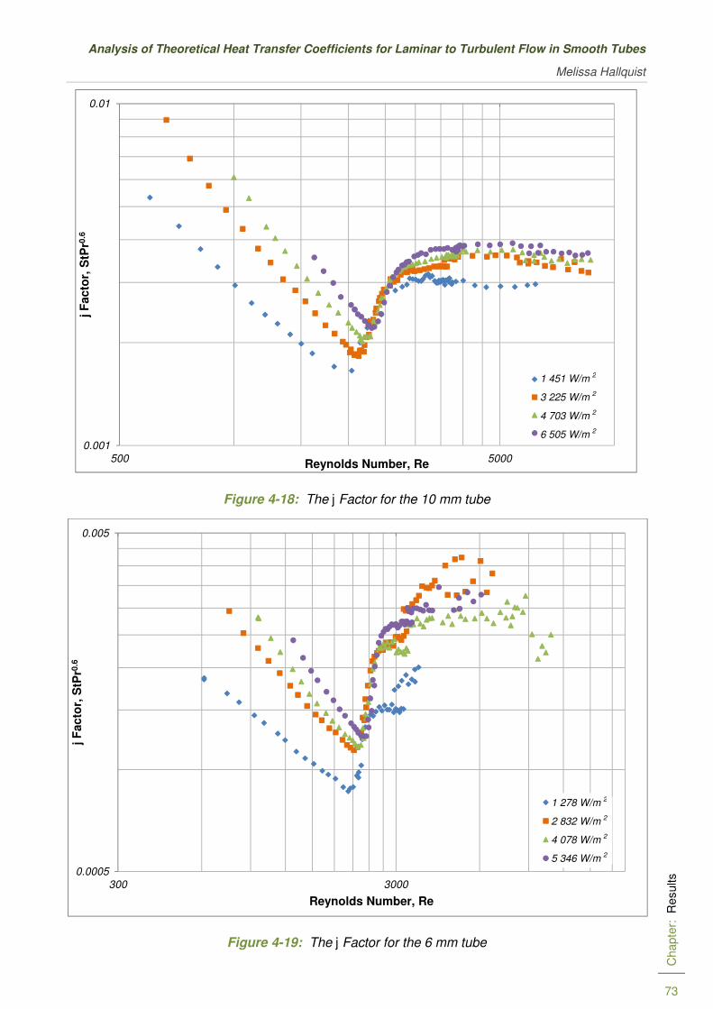
Analysis of Theoretical Heat Transfer Coefficients for Laminar to Turbulent Flow in Smooth Tubes
Melissa Hallquist
Chapte
r: R
esults
73
Figure 4-18: The j Factor for the 10 mm tube
Figure 4-19: The j Factor for the 6 mm tube
0.001
0.01
500 5000
j F
acto
r, S
tPr0
.6
Reynolds Number, Re
1 451 W/m
3 225 W/m
4 703 W/m
6 505 W/m
0.0005
0.005
300 3000
j F
acto
r, S
tPr0
.6
Reynolds Number, Re
1 278 W/m
2 832 W/m
4 078 W/m
5 346 W/m
1 451 W/m 2
3 225 W/m 2
4 703 W/m 2
6 505 W/m 2
1 278 W/m 2
2 832 W/m 2
4 078 W/m 2
5 346 W/m 2

University of Pretoria
Department of Mechanical and Aeronautical Engineering
Chapte
r: R
esults
74
The results converge during transition with a change in gradient marking the onset of turbulence. The Reynolds range of transition is the same in each of the heat flux cases, resulting in a delay in the onset of turbulence with increasing heat flux.
Figure 4-20: Stanton number for the 8 mm tube
In the turbulent regime, the higher the heat flux, the higher the j factor. In both the 10 mm and 8 mm test case, the results of the lowest heat flux case breaks away from the other results. In the 6 mm results, the Stanton number does not decrease but instead scattering occurs with data points higher than the other results.
4.3.5 CONCLUSIONS
This chapter considered all the measured results and described the trends observed. Based on both the friction factor and Nusselt number results, it was determined that transition is a smooth process from laminar to turbulent flow and therefore can be accurately described for design purposes. The onset of transition is a function of the heat flux of the system and occurs between a Reynolds number of 2 100 to 2 400.
Based on the flow regime map developed by Metais and Eckert (1964) and the Gr/Re2 parameter, it should be concluded that none of the recorded results are significantly influenced by natural convection. However, when the local heat transfer ratio between the top and the bottom of the tube is considered, it can be concluded that secondary flow effects are a contributing factor in laminar flow and to a smaller extent in transitional flow as well.
The fully developed Nusselt number was compared with the average Nusselt numbers to determine the differences (if any) between their profiles. In the laminar and turbulent regimes, the fully developed Nusselt number is higher than the average Nusselt number. Transition for
0.001
0.01
500 5000
j F
acto
r, S
tPr0
.6
Reynolds Number, Re
1 464 W/m
3 192 W/m
4 575 W/m
6 271 W/m
1 464 W/m 2
3 192 W/m 2
4 575 W/m 2
6 271 W/m 2

Analysis of Theoretical Heat Transfer Coefficients for Laminar to Turbulent Flow in Smooth Tubes
Melissa Hallquist
Chapte
r: R
esults
75
each heat flux case occurs at the same Reynolds number as with the average Nusselt numbers.
The j factor was the final parameter discussed to further understand the behaviour of the flow conditions. The same transition positions were observed with the results converging onto a single line over the transitional flow region. The laminar results demonstrate a dependence on the heat flux of the system. As the heat flux is increased, the results shift higher.

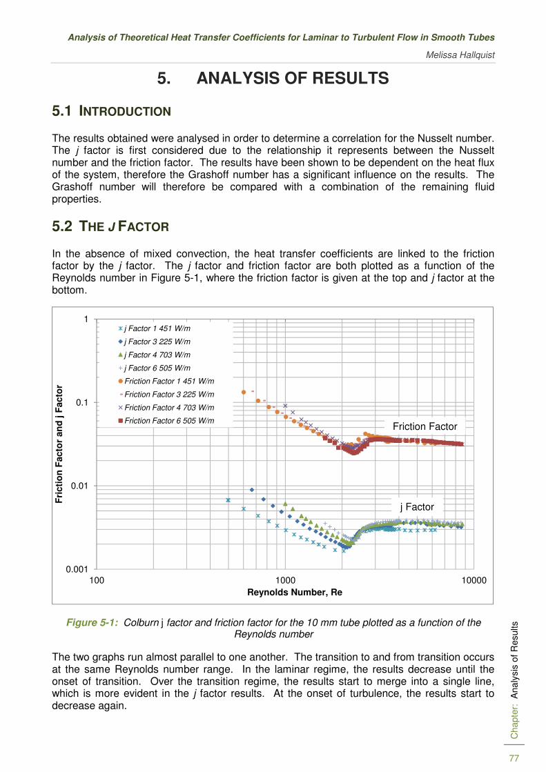
Analysis of Theoretical Heat Transfer Coefficients for Laminar to Turbulent Flow in Smooth Tubes
Melissa Hallquist
Chapte
r:
Ana
lysis
of R
esults
77
5. ANALYSIS OF RESULTS
5.1 INTRODUCTION
The results obtained were analysed in order to determine a correlation for the Nusselt number. The j factor is first considered due to the relationship it represents between the Nusselt number and the friction factor. The results have been shown to be dependent on the heat flux of the system, therefore the Grashoff number has a significant influence on the results. The Grashoff number will therefore be compared with a combination of the remaining fluid properties.
5.2 THE J FACTOR
In the absence of mixed convection, the heat transfer coefficients are linked to the friction factor by the j factor. The j factor and friction factor are both plotted as a function of the Reynolds number in Figure 5-1, where the friction factor is given at the top and j factor at the bottom.
Figure 5-1: Colburn j factor and friction factor for the 10 mm tube plotted as a function of the Reynolds number
The two graphs run almost parallel to one another. The transition to and from transition occurs at the same Reynolds number range. In the laminar regime, the results decrease until the onset of transition. Over the transition regime, the results start to merge into a single line, which is more evident in the j factor results. At the onset of turbulence, the results start to decrease again.
0.001
0.01
0.1
1
100 1000 10000
Fri
cti
on
Facto
r an
d j F
acto
r
Reynolds Number, Re
j Factor 1 451 W/m
j Factor 3 225 W/m
j Factor 4 703 W/m
j Factor 6 505 W/m
Friction Factor 1 451 W/m
Friction Factor 3 225 W/m
Friction Factor 4 703 W/m
Friction Factor 6 505 W/mFriction Factor
j Factor

University of Pretoria
Department of Mechanical and Aeronautical Engineering
Chapte
r:
Ana
lysis
of R
esults
78
In an attempt to collapse all the results onto a single line, the j factor is multiplied by a factor of 4Pr2/3 (Olivier & Meyer 2010) with the results shown in Figure 5-2.
Figure 5-2: Corrected Colburn j factor and friction factor for the 10 mm tube plotted as a function of the Reynolds number
The results do start to merge with one another, but not sufficiently enough for an accurate correlation to be developed. The laminar results are too varied with a definite increase in the j factor with increasing heat flux. In the turbulent flow regime, the results of the j factor over shoot the friction factor results by approximately 0.02 (an increase of approximately 50%).
Despite the differences in the laminar and turbulent regimes, the transitional flow regime does show a closer approximation between the j factor and the friction factor. This regime was isolated and the multiplication factor adjusted in order to determine whether a correlation could be found for this flow regime.
Figure 5-3 shows the results of the Nusselt number using the correction factor suggested by Olivier and Meyer (2010), where the resulting equation would be:
8
32 fPrSt
/ = (50)
The figure illustrates the 100% Nusselt number prediction (shown in red) with an error band of 10% above and below this ideal (shown in green). The prediction of the Nusselt number does not follow the correct gradient with the errors increasing for increased Nusselt number. This suggests that the correction factor should be higher in order to improve the prediction across the full Nusselt number range. The factor 4 was increased to 4.7, with the results given in Figure 5-4.
0.01
0.1
1
100 1000 10000
Fri
cti
on
Facto
r an
d C
co
rrecte
d j
Facto
r
Reynolds Number, Re
j Factor 1 451 W/m
j Factor 3 225 W/m
j Factor 4 703 W/m
j Factor 6 505 W/m
Friction Factor 1 451 W/m
Friction Factor 3 225 W/m
Friction Factor 4 703 W/m
Friction Factor 6 505 W/m

Analysis of Theoretical Heat Transfer Coefficients for Laminar to Turbulent Flow in Smooth Tubes
Melissa Hallquist
Chapte
r:
Ana
lysis
of R
esults
79
Figure 5-3: Corrected Colburn j factor (4Pr2/3) and friction factor for the 10 mm tube plotted as a function of the Reynolds number
Figure 5-4: Corrected Colburn j factor (4.7Pr2/3) and friction factor for the 10 mm tube plotted as a function of the Reynolds number
These results are more promising, with 75% of the data falling within the 10% error bands. As this factor is increased, the gradient of the Nusselt number prediction increases capturing
0
5
10
15
20
25
30
0 5 10 15 20 25 30
Pre
dic
ted
Nu
sselt
Nu
mb
er
Measured Nusselt Number
Series1
Series2
0
5
10
15
20
25
30
0 5 10 15 20 25 30
Pre
dic
ted
Nu
sselt
Nu
mb
er
Measured Nusselt Number
Series1
Series2
+10 %
-10 %
Measurements
Nu prediction (equation 50)
Measurements
Nu prediction (equation 50 with a factor of 4.7)
+10 %
-10 %

University of Pretoria
Department of Mechanical and Aeronautical Engineering
Chapte
r:
Ana
lysis
of R
esults
80
more of the data at the higher Nusselt number range. However, if the factor is increased too much, the representation of the Nusselt number at the onset of turbulence is diminished.
This model was now applied to the other two test sections, with disappointing results.
Figure 5-5: Corrected Colburn j factor (4.7Pr2/3) and friction factor for the 6 mm tube plotted as a function of the Reynolds number
The 6 mm results (Figure 5-5) are not well represented by this correlation. The prediction for the first half of the Nusselt number is approximately three times the Nusselt number measured. The gradient of the Nusselt number in this case is a lot lower illustrated by the flat profile of the measurements. This indicates that a smaller correction factor is required to improve the prediction of this correlation. It should be noted that the results of the 6 mm test section is subject to the highest uncertainties and therefore could prove unreliable in terms of defining a correlation.
The results of the 8 mm test section are given in Figure 5-6. These results are also not well predicted by the correlation, with only 40% of the data falling within the 10% error bands. These results show a flatter profile than that which the ideal Nusselt number correlation predicts.
When all three test cases are considered it would suggest that the multiplication factor is dependent of the tube size under consideration. With only three test section sizes considered in this study, there is not enough data in order to determine the influence the tube size would have on an overall correlation.
0
2
4
6
8
10
12
14
16
18
0 2 4 6 8 10 12 14 16 18
Pre
dic
ted
Nu
sselt
Nu
mb
er
Measured Nusselt Number
Series1
Series2
+10 %
-10 %
Measurements
Nu prediction (equation 50 with a factor of 4.7)

Analysis of Theoretical Heat Transfer Coefficients for Laminar to Turbulent Flow in Smooth Tubes
Melissa Hallquist
Chapte
r:
Ana
lysis
of R
esults
81
Figure 5-6: Corrected Colburn j factor (4.7Pr2/3) and friction factor for the 8 mm tube plotted as a function of the Reynolds number
5.3 GRASHOFF NUMBER
For the initial analysis, the Grashoff number was plotted on the y-axis in order to capture the secondary flow effects. The basic form of the Nusselt number equation for turbulent flow was used for the x-axis:
Nux
w
14.0
4.08.0PrRe
=µ
µ
(51)
Once the measurements reach fully developed turbulent flow, there are no more secondary flow effects, which would result in no gradient in the curve. The results of the 10 mm tube are shown in Figure 5-7 plotted on a log-log scale.
There are four regimes evident in Figure 5-7: laminar, transition, developing turbulent flow and fully developed turbulent flow. For identification purposes, the 6 505 W/m2 was marked by the letters A to E to illustrate these different regimes.
In general, as the flow rate increase,s the Grashoff number decreases because the temperature differential between the wall and fluid decreases. This decrease in temperature differential also results in a decrease in the viscosity ration.
In the laminar flow regime (A to B), the decrease in the Grashoff number can be described by a straight line, where the gradient of this line is the same for each of the heat flux cases. This straight line suggests that the data for this flow regime can be described by a power function
0
5
10
15
20
25
30
0 5 10 15 20 25 30
Pre
dic
ted
Nu
sselt
Nn
um
ber
Measured Nusselt Number
Series1
Series2
Measurements
Nu prediction (equation 50 with a factor of 4.7) +10 %
-10 %

University of Pretoria
Department of Mechanical and Aeronautical Engineering
Chapte
r:
Ana
lysis
of R
esults
82
(y=axb). The gradient of the straight line is the same for each of the heat flux cases, suggesting a constant exponent (b) independent of the heat flux on the system. As the heat flux decreases, the curve is lower suggesting that the coefficient in the power function is dependent on the heat flux of the system. As the heat flux increases, the coefficient increases.
Figure 5-7: Grashoff number for the 10 mm results given as a function of the Reynolds number, viscosity ratio and Nusselt number
A gradient change marks the onset of transition flow (B to C). As with the laminar results, the gradient of the transition results is the same for different heat flux values. The gradient in the lowest heat flux is slightly different from the others, with scattering evident in the data. The uncertainties for this test case are high and due to the deviation from the other data sets, the lowest heat flux cases will not be considered in the development of a correlation.
The transition results can also be approximated by a straight line with a negative gradient (y=ax-b). This suggests that a power curve can fit the data where the coefficient decreases for decreasing heat flux.
There is a slight change in gradient as the flow becomes turbulent. These initial turbulent results (C to D) have a decreasing gradient. If the lowest heat flux case is neglected as with the transitional results, the gradient of the developing turbulent results is equal.
Once the flow is fully developed, there are no longer any secondary flow effects and therefore the results form a straight vertical line (D to E). This line decreases along the x-axis as the heat flux increases.
1.E+02
1.E+03
1.E+04
1.E+05
1.E+01 1.E+02 1.E+03
Gra
sh
off
Nu
mb
er
[Gr]
Re0.8Pr0.4 (µ/µw)0.14Nu-1
1 451 W/m
3 225 W/m
4 703 W/m
6 505 W/m
A
B
C
D
E
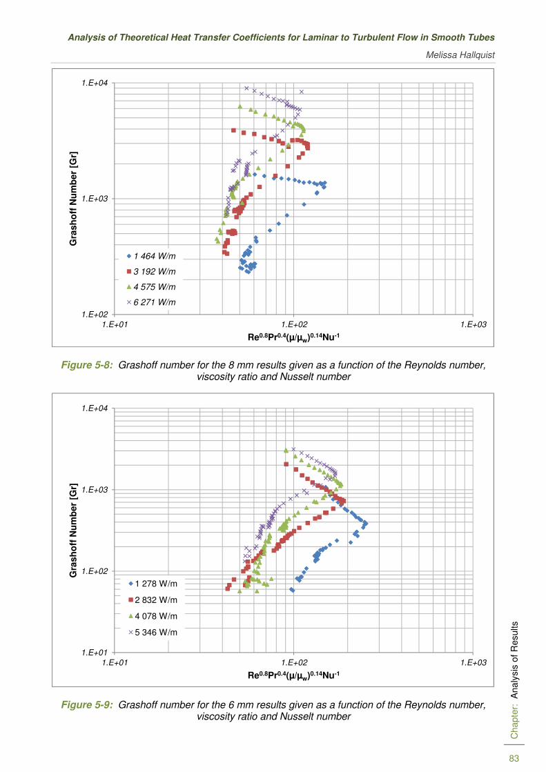
Analysis of Theoretical Heat Transfer Coefficients for Laminar to Turbulent Flow in Smooth Tubes
Melissa Hallquist
Chapte
r:
Ana
lysis
of R
esults
83
Figure 5-8: Grashoff number for the 8 mm results given as a function of the Reynolds number, viscosity ratio and Nusselt number
Figure 5-9: Grashoff number for the 6 mm results given as a function of the Reynolds number, viscosity ratio and Nusselt number
1.E+02
1.E+03
1.E+04
1.E+01 1.E+02 1.E+03
Gra
sh
off
Nu
mb
er
[Gr]
Re0.8Pr0.4(µ/µw)0.14Nu-1
1 464 W/m
3 192 W/m
4 575 W/m
6 271 W/m
1.E+01
1.E+02
1.E+03
1.E+04
1.E+01 1.E+02 1.E+03
Gra
sh
off
Nu
mb
er
[Gr]
Re0.8Pr0.4(µ/µw)0.14Nu-1
1 278 W/m
2 832 W/m
4 078 W/m
5 346 W/m

University of Pretoria
Department of Mechanical and Aeronautical Engineering
Chapte
r:
Ana
lysis
of R
esults
84
The results of the other two test sections are given in Figure 5-8 and Figure 5-9. As the tube size decreases, the Grashoff number decreases and the x-axis shifts to the right. In each of the test cases, the same gradient is seen in each of the heat flux cases. The difficulty is determining a common gradient that will suit all three test sections.
In the laminar flow regime, the gradient of the 6 mm test case is approximately -1.31. For the 10 mm test case, however, this value changes to -0.77 and in the 8 mm test case, the gradient is -0.57. These gradients are related to the tube diameter but there is insufficient data to determine what the correlation is. The same can be said for the transitional regime where the gradients are 1.35, 1.23 and 0.3 for the different test cases.
A factor dependent on the heat flux of the system needs to be applied to the data in order for the data to collapse on a single curve. This factor would have to minimise the effect of the Grashoff number and is not necessarily the same for each of the flow regimes and therefore the data was isolated and each of the flow regimes considered separately.
The transitional flow regime is considered first. The coefficients of the factors in the y-axis were adjusted and the effect of the Grashoff number reduced in order to determine a best-fit curve for all the heat flux cases. The Prandtl number is also dependent on the heat flux of the system and therefore it was plotted on the y-axis instead in order for it to be adjusted accordingly. The results of the 8 mm are given in Figure 5-10.
Figure 5-10: Curve fit for the 8 mm transitional flow data
The coefficients were determined experimentally by adjusting them in different combinations until the best curve fit could be determined. As discussed earlier in this section, a power function best describes the trend in the data. The results of the different heat flux cases converge closely with 77% of the data described by the correlation. The 6 mm and 10 mm results were also plotted with the same axis combination, with the results shown in Figure 5-11 and Figure 5-12 respectively.
y = 10.374x0.0777
R² = 0.7732
10
100
1 10
Gr0
.085P
r
Re0.5(µ/µw)0.14Nu-1

Analysis of Theoretical Heat Transfer Coefficients for Laminar to Turbulent Flow in Smooth Tubes
Melissa Hallquist
Chapte
r:
Ana
lysis
of R
esults
85
Figure 5-11: Curve fit for the 6 mm transitional flow data
Figure 5-12: Curve fit for the 10 mm transitional flow data
The curve fit in these cases is not as accurate as that seen in the 8 mm tube with only 16.4% of the data in the 10 mm tube captured by the curve fit. The exponent in each of the cases is similar suggesting that an average exponent between the different tube sizes could be found. The coefficient of the curve fit is dependent on the tube diameter with the coefficient increasing
y = 9.3799x0.0619
R² = 0.5528
5
50
1 10
Gr0
.085P
r
Re0.5(µ/µw)0.14Nu-1
y = 11.98x0.0612
R² = 0.1642
1
10
100
1 10
Gr0
.085P
r
Re0.5(µ/µw)0.14Nu-1
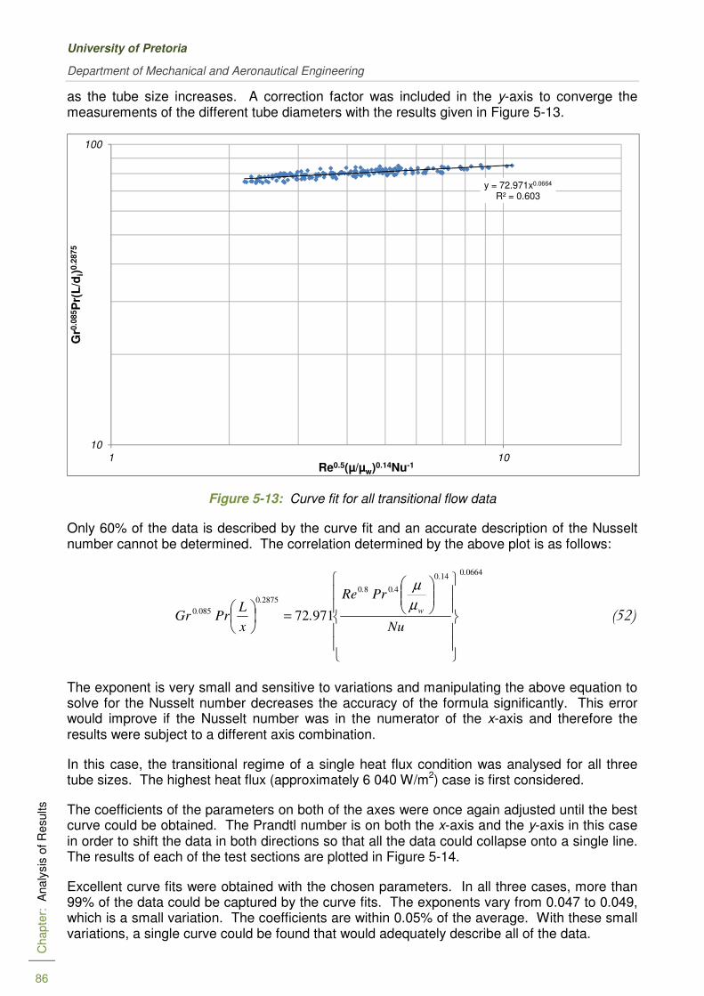
University of Pretoria
Department of Mechanical and Aeronautical Engineering
Chapte
r:
Ana
lysis
of R
esults
86
as the tube size increases. A correction factor was included in the y-axis to converge the measurements of the different tube diameters with the results given in Figure 5-13.
Figure 5-13: Curve fit for all transitional flow data
Only 60% of the data is described by the curve fit and an accurate description of the Nusselt number cannot be determined. The correlation determined by the above plot is as follows:
06640140
4080
28750
085097172
..
w
..
.
.
Nu
PrRe
.x
LPrGr
=
µ
µ
(52)
The exponent is very small and sensitive to variations and manipulating the above equation to solve for the Nusselt number decreases the accuracy of the formula significantly. This error would improve if the Nusselt number was in the numerator of the x-axis and therefore the results were subject to a different axis combination.
In this case, the transitional regime of a single heat flux condition was analysed for all three tube sizes. The highest heat flux (approximately 6 040 W/m2) case is first considered.
The coefficients of the parameters on both of the axes were once again adjusted until the best curve could be obtained. The Prandtl number is on both the x-axis and the y-axis in this case in order to shift the data in both directions so that all the data could collapse onto a single line. The results of each of the test sections are plotted in Figure 5-14.
Excellent curve fits were obtained with the chosen parameters. In all three cases, more than 99% of the data could be captured by the curve fits. The exponents vary from 0.047 to 0.049, which is a small variation. The coefficients are within 0.05% of the average. With these small variations, a single curve could be found that would adequately describe all of the data.
y = 72.971x0.0664
R² = 0.603
10
100
1 10
Gr0
.085P
r(L
/di)
0.2
875
Re0.5(µ/µw)0.14Nu-1

Analysis of Theoretical Heat Transfer Coefficients for Laminar to Turbulent Flow in Smooth Tubes
Melissa Hallquist
Chapte
r:
Ana
lysis
of R
esults
87
Figure 5-14: Curve fit for the different test cases at the highest heat flux condition
Figure 5-15: A correlation for the results of the highest heat flux condition
y = 5.71759x-0.04943
R² = 0.99475
y = 5.71926x-0.04813
R² = 0.99430
y = 5.71198x-0.04723
R² = 0.99937
5.9
5.95
6
6.05
6.1
6.15
6.2
6.25
6.3
6.35
0 0.05 0.1 0.15 0.2 0.25 0.3 0.35 0.4 0.45 0.5
Gr0
.045P
r0.2
(L/d
i)0.1
625
Re0.45Pr0.2(µ/µw)0.14Nu-1
10mm Tube
8mm Tube
6mm Tube
y = 5.73935x-0.04502
R² = 0.99017
5.9
5.95
6
6.05
6.1
6.15
6.2
6.25
6.3
6.35
0 0.05 0.1 0.15 0.2 0.25 0.3 0.35 0.4 0.45 0.5
Gr0
.045P
r0.2
(L/d
i)0.1
625
Re0.45Pr0.2(µ/µw)0.14Nu-1

University of Pretoria
Department of Mechanical and Aeronautical Engineering
Chapte
r:
Ana
lysis
of R
esults
88
The results of the curve fit are shown in Figure 5-15 and based on these results, the following correlation was determined:
045020
140
20450
16250
200450739355
.
.
w
..
.
..
PrRe
Nu.
x
LPrGr
−
=
µ
µ (52a)
From which the Nusselt number can be determined as:
63
2417
140
450
103931
.
.
.
w
.
x
LPrGre.
Re
Nu
=−
µ
µ
(52b)
The Nusselt number for these cases was determined based on the above correlation with promising results. Figure 5-16 illustrates the calculated Nusselt number against the measured Nusselt number. The ideal solution is shown by the solid green line and a ±10% error band by the dashed lines. The average error between the calculated and measured Nusselt number is 2.8% with none of the results lying outside of the 10% error bands.
Figure 5-16: Evaluation of the correlation for the highest heat flux case
The same approach was taken with the other heat flux cases with the exception of the lowest case. The 1 400 W/m2 cases were excluded due to the elevated uncertainties inherent in these test cases.
0
5
10
15
20
25
30
0 5 10 15 20 25 30
Calc
ula
ted
Nu
sselt
Nu
mb
er
Measured Nusselt Number
Series1
Series4
+10 %
-10 %
Measurements
Nu prediction (equation 52)

Analysis of Theoretical Heat Transfer Coefficients for Laminar to Turbulent Flow in Smooth Tubes
Melissa Hallquist
Chapte
r:
Ana
lysis
of R
esults
89
Figure 5-17 gives the curve fit for the 4 450 W/m2 heat flux cases where 99% of the data is described by the curve fit. The form of the equation is the same as the previous heat flux condition with variations in the exponent and the coefficient.
Figure 5-17: A correlation for an average heat flux of 4 450 W/m2
As with the higher heat flux case, all of the results lie within a 10% error band with the average error in the Nusselt number being 0.86%. The resulting correlation is as follows:
048190
140
20450
16250
200450657995
.
.
w
..
.
..
PrRe
Nu.
x
LPrGr
−
=
µ
µ (53a)
From which the Nusselt number can be determined as:
373
953934016
140
450
104062
.
..
.
w
.
x
LPrGre.
Re
Nu
=−
µ
µ
(53b)
y = 5.65799x-0.04819
R² = 0.99899
5.8
5.85
5.9
5.95
6
6.05
6.1
6.15
6.2
6.25
6.3
0 0.05 0.1 0.15 0.2 0.25 0.3 0.35 0.4 0.45 0.5
Gr0
.045P
r0.2
(L/d
i)0.1
625
Re0.45Pr0.2(µ/µw)0.14Nu-1

University of Pretoria
Department of Mechanical and Aeronautical Engineering
Chapte
r:
Ana
lysis
of R
esults
90
The final case considered is for an average heat flux of 3 080 W/m2 shown in Figure 5-18. The resulting correlation with an average Nusselt number error of 3.1% is as follows:
0489910
140
20450
16250
200450566665
.
.
w
..
.
..
PrRe
Nu.
x
LPrGr
−
=
µ
µ (54a)
where
323
8839185016
140
450
1024
.
..
.
w
.
x
LPrGre.
Re
Nu
=−
µ
µ
(54b)
Figure 5-18: A correlation for an average heat flux of 3 080 W/m2
In each of the cases considered, a very good correlation, which described the Nusselt number to within 10% of the values measured could be found. As the heat flux increases, the coefficient of the power function increases from 5.57 for the 3 080 W/m2 case to 5.74 for the highest heat flux case (a 3% spread). The average of the three cases is approximately 5.65, which corresponds to the coefficient of the 4 450 W/m2 heat flux case.
y = 5.56666x-0.04991
R² = 0.98844
5.7
5.75
5.8
5.85
5.9
5.95
6
6.05
6.1
6.15
6.2
6.25
0 0.05 0.1 0.15 0.2 0.25 0.3 0.35 0.4 0.45 0.5
Gr0
.045P
r0.2
(L/d
i)0.1
625
Re0.45Pr0.2(µ/µw)0.14Nu-1
Analysis of Theoretical Heat Transfer Coefficients for Laminar to Turbulent Flow in Smooth Tubes
Melissa Hallquist
Chapte
r:
Ana
lysis
of R
esults
91
The coefficients of the power functions also vary between the different heat flux cases considered. The average coefficient is approximately 0.048, which once again corresponds to the 4 450 W/m2 heat flux case.
The variance in the coefficient is approximately 10%, but applying this correlation to the other test cases does not capture the behaviour of the Nusselt number correctly. Plotting all three of these test cases on the same figure shows three distinct lines separated by approximately 5%. Therefore, using an average of the three curve fits will capture the overall shape of the Nusselt number but the accuracy will vary as the heat flux is varied.
More heat flux cases are required to determine the relationship between the exponents and coefficients of this proposed power function.
5.4 SUMMARY
In this chapter, the results were analysed in an attempt to determine a correlation for the Nusselt number as a function of the flow rate for the various test cases considered. Despite obvious trends discovered in the results, there is insufficient data to develop a correlation that would accurately describe all of the test cases across all of the flow regimes. By splitting the regimes, a correlation can be found for each of the test sections, however, further data is required to obtain a correlation for different tube diameters.
The results were first analysed by comparing the j factor to the friction factor. Based on literature, the j factor was multiplied by a factor of 4 in order to determine whether the j factor and friction factor results would converge. The results did start to converge, however, the factor had to be altered for each of the test cases to improve the convergence. In addition, secondary flow effects resulted in variations in the laminar results of the j factor, which were not captured in the friction factor results.
In order to capture secondary flow effects, the Grashoff number was plotted on the y-axis with a common turbulent Nusselt number equation represented on the x-axis. Four distinct regimes were identified in this plot: laminar, transition, developing turbulent and fully developed turbulent flow. For each of these flow regimes, a constant gradient could be identified among the different heat flux conditions. This constant was different for each of the test cases and more data is required in order to determine the correlation between the constant and tube diameters.
To further understand the flow characteristics, the transitional flow regime was isolated for each of the test cases to determine whether a correlation could be found for this regime. The coefficients of the different parameters were adjusted until a best-fit curve could be obtained. Very good correlations could be found for individual heat flux cases across the different test tube diameters. However, the accuracy is diminished when the correlation is applied to all the test cases considered.


Analysis of Theoretical Heat Transfer Coefficients for Laminar to Turbulent Flow in Smooth Tubes
Melissa Hallquist
Chapte
r:
Sum
mary
, C
onclu
sio
ns a
nd R
ecom
men
dations
93
6. SUMMARY, CONCLUSIONS AND RECOMMENDATIONS
6.1 SUMMARY
The purpose of this study was to expand the knowledge of the behaviour of heated flow transfer in the transitional regime. Although little is known of this regime, heat exchangers are often forced to operate under these conditions due to space constraints and/or changes in operating conditions. With little knowledge about this regime, the efficiency of these heat exchangers cannot be predicted.
A few studies have already been conducted with regards to the transitional flow regime mainly focusing on the entrance flow effects. The correlation determined by Olivier and Meyer (2010) predicts 88% of the results in their experiments well, however, the correlation is specific to the uniform temperature boundary considered. The correlations developed by Ghajar and Tam (1994) are for the local Nusselt number and are therefore cumbersome to apply to an overall heat exchange analysis.
This study considered three different heat exchangers, each subject to four different heat flux conditions. Smaller tube diameters were considered to decrease the thermal developing length of the system. The test set-up consisted of an overall system supplying water to a removable test section with a direct current welder that heats the fluid flowing through the test section. There were three types of Nusselt numbers to be considered in this study, namely the local, average and fully developed Nusselt numbers. The system was subject to an uncertainty analysis and all the errors were considered to be within reasonable limits as was shown by the system validation. It was therefore concluded that the experimental set-up should generate accurate measurements of the heat transfer coefficient and friction factors in the transitional regime.
Based on both the friction factor and Nusselt number results, it has been determined that transition is a smooth process from laminar to turbulent flow and therefore can be accurately described for design purposes. The onset of transition occurs between a Reynolds number of 2 100 and 2 400 depending on the heat flux of the system. As the heat flux was increased, the transition point increased. This phenomenon was validated by the friction factor results, which yielded the same transition values.
6.2 CONCLUSIONS
Based on a flow regime map developed in literature and the Gr/Re2 parameter, it should be concluded that none of the recorded results are significantly influenced by natural convection, however, some trends in the data contradict this conclusion.
The friction factor in the laminar regime is higher for increasing heat flux, which is due to the influence of the viscosity ratio (and therefore suggests a secondary flow influence). The local Nusselt number should approach a flat profile once thermally fully developed. This was not the case in the results presented. This suggests another influence in the flow behaviour, which could be attributed to secondary flow. In each of the test cases, the Nusselt number initially decreases with increasing Reynolds number, which must be attributed to the influence of the Grashoff number (as highlighted in Chapter 2).
After presenting all of the results obtained, an analysis was conducted in order to determine if the patterns observed could be described by a correlation. The friction factor and j factor

University of Pretoria
Department of Mechanical and Aeronautical Engineering
Chapte
r:
Sum
mary
, C
onclu
sio
ns a
nd R
ecom
men
dations
94
results are parallel to one another and a factor was applied to the j factor to attempt to collapse the data onto a single curve. The transition results come close to one another, however, a universal factor between the different test cases could not be found. In addition, the laminar results of the j factor do not correspond to the friction factor results. This variation is attributed to secondary flow effects not captured by the friction factor measurements.
The Grashoff numbers were described as a function of the relevant heat transfer parameters. Four distinct flow regimes could be identified and for each of the regimes, a common constant between the different heat flux cases was identified. Due to the sharp changes in gradient (specifically between the laminar and transitional flow regimes) a different correlation would have to be found for each regime.
The analysis was restricted to the transitional flow regime where the different heat fluxes of an individual test case were first investigated. The influence of the Grashoff number had to be reduced in an attempt to collapse the data onto a single curve. Based on this, an attempt was made to collapse the different heat flux cases onto a single line. This could be achieved with varying accuracies across the different tube sizes. When combining all the data onto a single curve, 60% of the data could be described by a power function. The Nusselt number is, however, described in the denominator of the x-axis and the exponents of the power function are very small and highly sensitive to fluctuations. The result is a poor correlation for the Nusselt number.
As a final attempt, a single heat flux case across all three test sections was analysed. Very good correlations for the individual heat flux cases could be found with accuracies in the Nusselt number as low as 0.86%. The coefficient and exponent of the power function varies with a variation in the heat flux applied to the system. More test cases are required in order to determine what this relationship is.
From this study, it can be concluded that with further data capturing, a correlation can be found to describe the Nusselt number in the transitional flow regime. There are discrepancies in the influence of secondary flow that requires further investigation.
6.3 RECOMMENDATIONS FOR FUTURE WORK
After completion of this study it was found that there are a number of areas that could be improved to further ensure accuracy of the results obtained. The data logger associated with this set-up does not take simultaneous readings but rather cycles through the data cards in sequence. In order to reduce testing time required, a different data capturing system could be used.
Although a DC arc welder provides a low-cost solution for a power supply, the power supplied by the welder is not uniform and required complex filters to be used by the control system in order to ensure that the correct boundary condition is met.
Calibration of the thermocouples should be conducted after connection to the test section, which requires a large thermal bath. Some measurement errors can be induced after connection to the tube wall. Four thermocouples are placed at each station to ensure this error is negligible, however, if secondary flow effects were to be mapped more reliability should be given to each thermocouple reading. Similarly, the pressure taps need to be calibrated after they are incorporated into the overall set-up. The system was calibrated with a water column, which provided accurate, stable measurements. The water column is a separate system and a new ‘zero’ point had to be established. An integrated calibration system would be more reliable and would avoid different ‘zero’ points for each diaphragm used.

Analysis of Theoretical Heat Transfer Coefficients for Laminar to Turbulent Flow in Smooth Tubes
Melissa Hallquist
Chapte
r:
Sum
mary
, C
onclu
sio
ns a
nd R
ecom
men
dations
95
The laboratory temperature should be monitored in order to accurately determine heat loss through the insulation.
A larger database is required before the phenomenon of transition can be accurately described. A larger range of heat flux conditions should be considered and a variety of fluids should be tested to determine the influence of the Prandtl number. The other two boundary conditions should also be tested over a variety of different heat transfer rates.


Analysis of Theoretical Heat Transfer Coefficients for Laminar to Turbulent Flow in Smooth Tubes
Melissa Hallquist
Chapte
r: R
efe
rences
97
7. REFERENCES
Allen, RW & Eckert, ERG 1964, 'Friction and heat transfer measurements to turbulent pipe
flow of water (Pr=7 and 8) at uniform wall heat flux', Journal of Heat Transfer, vol 86, pp.
301-310.
ASHRAE 2009, 2009 ASHRAE Handbook - Fundamentals (SI Edition), American Society
of Heating, Refrigerating and Air-Conditioning Engineers, Inc.
Cengel, YA 2006, Heat and mass transfer - A practical approach, 3rd edn, Mc Graw Hill,
New York City.
Churchill, SW 1977, 'Comprehensive correlating equations for heat, mass and momentum
transfer in fully developed flow in smooth tubes', Industrial Engineering and Chemistry
Fundamentals, vol 16, no. 1, pp. 109-116.
Colburn, AP 1933, 'Mean temperature difference and heat transfer coefficient in liquid heat
exchangers', Industrial Engineering Chemistry, vol 25, no. 8, pp. 873-877.
Dittus, FW & Boelter, LM 1930, 'Heat transfer in automobile radiators of the tubular type',
International Communication of Heat and Mass Transfer, vol 12, pp. 3-22.
Engineering Science Data Unit (ESDU) 1993, 'Forced convection heat transfer in straight
tubes part 1', IHS Standard, no. 92003.
Engineering Science Data Unit (ESDU) 2001, 'Forced convection heat transfer in straight
tubes part 2', IHS Standard, no. 93018.
Garcia, A, Vicent, PG & Viedma, A 2005, 'Experimental study of heat transfer
enhancement with wire coil inserts in laminar-transition-turbulent regimes at different
Prandtl numbers', International Journal of Heat and Mass Transfer, vol 45, pp. 4640-4651.
Ghajar, AJ & Madon, KF 1992, 'Pressure drop measurements in the transition region for a
circular tube with three different inlet configurations', Experimental Thermal and Fluid
Science, vol 5, pp. 129-135.
Ghajar, AJ & Tam, LM 1994, 'Heat transfer measurements and correlations in the
transition region for a circular tube with three different inlet configurations', Experimental
Thermal and Fluid Sciences, vol 8, pp. 79-90.
Ghajar, AJ & Tam, LP 1995, 'Flow regime map for a horizontal pipe with a uniform wall
heat flux and three inlet configurations', Experimental Thermal and Fluid Sciences, vol 10,
pp. 287-297.
Gnielinski, V 1976, 'New equations for heat and mass transfer in turbulent pipe and
channel flow', International Chemical Engineering, vol 16, no. 2, pp. 359-368.

University of Pretoria
Department of Mechanical and Aeronautical Engineering
Chapte
r: R
efe
rences
98
Kline, SJ & McClintock, FA 1953, 'Describing uncertainties in single sample experiments',
Mechanical Engineering, vol 75, no. 1, pp. 3-8.
Kreith, F & Bohn, MS 2001, Principles of heat transfer, 6th edn, Brooks/Cole, USA.
Lienhard, JH & Lienhard, JH 2008, A heat transfer textbook, 3rd edn, Phlogiston,
Cambridge, Massachusetts.
Metais, B & Eckert, ERG 1964, 'Forced, mixed and free convection regimes', Journal of
Heat Transfer, vol 86, pp. 295-296.
Meyer, JP & Du Preez, A 2010, 'Heat transfer and pressre drop characteristics of water in
the transitional flow regime of horzontal smooth tubes at constant wall temperature',
Proceedings of the 14th International Heat Transfer Conference, IHTC-14, no. IHTC14-
22340, pp. 8-13.
Meyer, JP & Olivier, JA 2011, 'Heat transfer in the transitional flow regime', Evaporation,
Condensation and Heat Transfer, pp. 245-260.
Mills, AF 1992, Heat Transfer, Richard D Irwin Inc, USA.
Mohammed, HA & Yasin, KS 2007, 'The effects of different entrance section lengths and
heating on free and forced convective heat transfer inside a horizontal circular tube',
International Communications in Heat and Mass Transfer, vol 34, pp. 769-784.
Olivier, JA & Meyer, JP 2010, 'Single-phase heat transfer and pressure drop of cooling of
water inside smooth tubes for transitional flow with different inlet geometries', HVAC & R
Research, vol 16, no. 4, pp. 471-496.
Petukhov, BS, Polyakov, AF & Strigin, BK 1969, 'Heat transfer in tubes with viscous-
gravity flow', Heat Transfer - Soviet Research, vol 1, no. 1, pp. 24-31.
Popiel, CO & Wojtkowiak, J 1998, 'Simple formulas for thermophysical properties of liquid
water for heat transfer calculations', Heat Transfer Engineering, vol 19, no. 3, pp. 87-101.
Rayle, RE 1959, 'Influence of orifice geometry on static pressure measurements', ASME,
no. Paper 59-A-234.
Shokouhmand, H & Salimpour, MR 2007, 'Optimal reynolds number of laminar forced
convection in a helical tube subject to uniform wall temperature', International
Communications in Heat & Mass Transfer, vol 34, pp. 753-761.
Sieder, EN & Tate, GE 1936, 'Heat transfer and pressure drop of liquids in tubes',
Industrial and Engineering Chemistry, vol 28, no. 12, pp. 1429-1435.
Sulliman, R, Liebenberg, L & Meyer, JP 2009, 'Improved flow pattern map for accurate
prediction of the heat transfer coefficients during condensation of R-134a in smooth

Analysis of Theoretical Heat Transfer Coefficients for Laminar to Turbulent Flow in Smooth Tubes
Melissa Hallquist
Chapte
r: R
efe
rences
99
horizontal tubes and within the low-mass flux range', International Journal of Heat and
Mass Transfer, vol 52, no. 25-26, pp. 5701-5711.
Van Rooyen, E, Christians-Lupi, M, Liebenberg, L & Meyer, JP 2010, 'Probabilistic flow-
pattern-based heat transfer correlation for condensing intermittent flow of refrigerants in
smooth horizontal tubes', International Journal of Heat and Mass Transfer, vol 53, no. 7-8,
pp. 1446-1460.
White, FM 2003, Fluid Mechanics, 5th edn, Mc Graw-Hill, New York.
Yilmaz, A 2008, 'Optimum length of heat transfer in turbulent tlow at constant wall
temperature', International Journal of Heat and Mass Transfer, vol 51, pp. 3478-3485.


Analysis of Theoretical Heat Transfer Coefficients for Laminar to Turbulent Flow in Smooth Tubes
Melissa Hallquist
101
Appendix A
UNCERTAINTIES
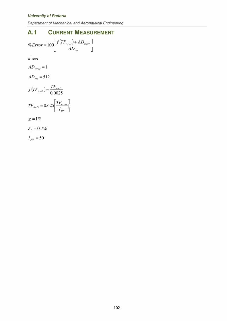
University of Pretoria
Department of Mechanical and Aeronautical Engineering
102
A.1 CURRENT MEASUREMENT
( )
+= −
res
errorDA
AD
ADTFfError% 100
where:
1=errorAD
512=resAD
( )00250.
TFTFf DA
DA−
− =
=−
PN
error
DAI
TF.TF 6250
%1=χ
%.L 70=ε
50=PNI

Analysis of Theoretical Heat Transfer Coefficients for Laminar to Turbulent Flow in Smooth Tubes
Melissa Hallquist
103
A.2 6MM TUBE RESULTS
A.2.1 FRICTION FACTOR
0.2
0.22
0.24
0.26
0.28
0.3
0.32
0.34
0.36
0.38
0 2000 4000 6000 8000 10000 12000
Fri
cti
on
Facto
r U
ncert
ain
ty [
%]
Reynolds Number, Re
1 278 W/m
2 832 W/m
4 078 W/m
5 346 W/m
1 278 W/m 2
2 832 W/m 2
4 078 W/m 2
5 346 W/m 2
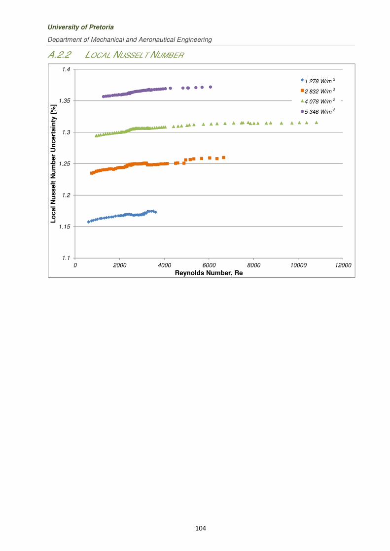
University of Pretoria
Department of Mechanical and Aeronautical Engineering
104
A.2.2 LOCAL NUSSELT NUMBER
1.1
1.15
1.2
1.25
1.3
1.35
1.4
0 2000 4000 6000 8000 10000 12000
Lo
cal N
usselt
Nu
mb
er
Un
cert
ain
ty [
%]
Reynolds Number, Re
1 278 W/m
2 832 W/m
4 078 W/m
5 346 W/m
1 278 W/m 2
2 832 W/m 2
4 078 W/m 2
5 346 W/m 2

Analysis of Theoretical Heat Transfer Coefficients for Laminar to Turbulent Flow in Smooth Tubes
Melissa Hallquist
105
A.2.3 AVERAGE NUSSELT NUMBER
1
1.02
1.04
1.06
1.08
1.1
1.12
1.14
1.16
1.18
1.2
0 2000 4000 6000 8000 10000 12000
Av
era
ge N
usselt
Nu
mb
er
Un
cert
ain
ty [
%]
Reynolds Number, Re
1 278 W/m
2 832 W/m
4 078 W/m
5 346 W/m
1 278 W/m 2
2 832 W/m 2
4 078 W/m 2
5 346 W/m 2

University of Pretoria
Department of Mechanical and Aeronautical Engineering
A.3 8MM TUBE RESULTS
A.3.1 FRICTION FACTOR
0
0.1
0.2
0.3
0.4
0.5
0.6
0.7
0 1000
Fri
cti
on
Facto
r U
ncert
ain
ty [
%]
rtment of Mechanical and Aeronautical Engineering
106
ESULTS
ACTOR
2000 3000 4000 5000Reynolds Number, Re
6000 7000
1 464 W/m
3 192 W/m
4 575 W/m
6 271 W/m
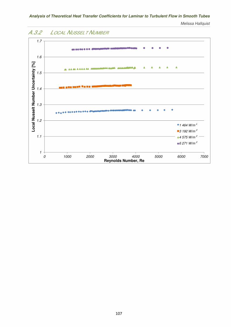
Analysis of Theoretical Heat Transfer Coefficients for Laminar to Turbulent Flow in Smooth Tubes
Melissa Hallquist
107
A.3.2 LOCAL NUSSELT NUMBER
1
1.1
1.2
1.3
1.4
1.5
1.6
1.7
0 1000 2000 3000 4000 5000 6000 7000
Lo
cal N
usselt
Nu
mb
er
Un
cert
ain
ty [
%]
Reynolds Number, Re
1 464 W/m
3 192 W/m
4 575 W/m
6 271 W/m
1 464 W/m 2
3 192 W/m 2
4 575 W/m 2
6 271 W/m 2
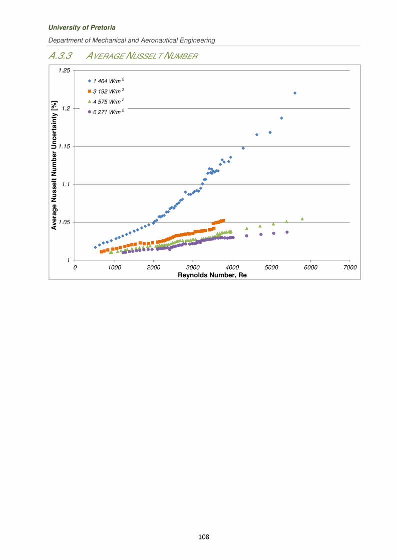
University of Pretoria
Department of Mechanical and Aeronautical Engineering
108
A.3.3 AVERAGE NUSSELT NUMBER
1
1.05
1.1
1.15
1.2
1.25
0 1000 2000 3000 4000 5000 6000 7000
Av
era
ge N
usselt
Nu
mb
er
Un
cert
ain
ty [
%]
Reynolds Number, Re
1 464 W/m
3 192 W/m
4 575 W/m
6 271 W/m
1 464 W/m 2
3 192 W/m 2
4 575 W/m 2
6 271 W/m 2

Analysis of Theoretical Heat Transfer Coefficients for Laminar to Turbulent Flow in Smooth Tubes
Melissa Hallquist
109
Appendix B
DATA REDUCTION SPREADSHEETS
This section includes a sample of each of the spreadsheets created in order to determine the necessary
properties from the measurements taken.

University of Pretoria
Department of Mechanical and Aeronautical Engineering
110
B.1 TUBE CHARACTERISTICS
B.1.1 6 MM TUBE
Test Tube Insulation
Tube Length [m] 5.7 Thermal Conductivity [W/m2K] 0.0374
Heated Length [m] 4.81 Insulation Thickness [m] 0.05
Thermocouple Interval [m] 0.36 Insulation Diameter [m] 0.107966
Entrance Length [m] 0.89 Insulation Thermal Resistance [K/W] 2.306128
Outer Tube Diameter [m] 0.007966
Inner Tube Diameter [m] 0.006071
Wall Thickness [m] 0.0009475
Outer Cross-Sectional Area [m2] 4.984E-05
Inner Cross-Sectional Area [m2] 2.895E-05
Total Outer-Surface Area [m2] 0.142647784
Total Inner-Surface Area [m2] 0.108713871
Heated Outer-Surface Area [m2] 0.120374709
Heated Inner-Surface Area [m2] 0.091739249
Cross-Sectional Area of Tube Wall [m2] 2.089E-05
Stainless Steel
Thermal Conductivity [W/m2K] 16.3
Thermal Resistance [K/W] 0.0005515
Resistivity (@ 20°C) [Ω·m] 7.40E-07
Thermal Coefficient [K-1] 0.003
Resistance (@ 20°C) [Ω] 0.170374

Analysis of Theoretical Heat Transfer Coefficients for Laminar to Turbulent Flow in Smooth Tubes
Melissa Hallquist
111
Steel Resistance
Thermocouple Position - 1 2 3 4 5 6 7 8 9 10 11 12 13 14 15
Thermocouple Position [m] 0.89 1.25 1.61 1.97 2.33 2.69 3.05 3.41 3.77 4.13 4.49 4.85 5.21 5.57 5.7
Placement [m] 0 0.36 0.72 1.08 1.44 1.8 2.16 2.52 2.88 3.24 3.6 3.96 4.32 4.68 4.99
Resistance (@ 20°C) [Ω] 0 0.013 0.026 0.038 0.051 0.064 0.077 0.089 0.102 0.115 0.128 0.140 0.153 0.166 0.177

University of Pretoria
Department of Mechanical and Aeronautical Engineering
112
B.1.2 8 MM TUBE
Test Tube Insulation
Tube Length [m] 5.7 Thermal Conductivity [W/m2K] 0.0374
Heated Length [m] 4.81 Insulation Thickness [m] 0.05
Thermocouple Interval [m] 0.36 Insulation Diameter [m] 0.107966
Entrance Length [m] 0.89 Insulation Thermal Resistance [K/W] 2.306128
Outer Tube Diameter [m] 0.007966
Inner Tube Diameter [m] 0.006071
Wall Thickness [m] 0.0009475
Outer Cross-Sectional Area [m2] 4.984E-05
Inner Cross-Sectional Area [m2] 2.895E-05
Total Outer-Surface Area [m2] 0.142647784
Total Inner-Surface Area [m2] 0.108713871
Heated Outer-Surface Area [m2] 0.120374709
Heated Inner-Surface Area [m2] 0.091739249
Cross-Sectional Area of Tube Wall [m2] 2.089E-05
Stainless Steel
Thermal Conductivity [W/m2K] 16.3
Thermal Resistance [K/W] 0.0004751
Resistivity (@ 20°C) [Ω·m] 7.40E-07
Thermal Coefficient [K-1] 0.003
Resistance (@ 20°C) [Ω] 0.119928

Analysis of Theoretical Heat Transfer Coefficients for Laminar to Turbulent Flow in Smooth Tubes
Melissa Hallquist
113
Steel Resistance
Thermocouple Position - 1 2 3 4 5 6 7 8 9 10 11 12 13 14 15
Thermocouple Position [m] 0.89 1.25 1.61 1.97 2.33 2.69 3.05 3.41 3.77 4.13 4.49 4.85 5.21 5.57 5.7
Placement [m] 0 0.36 0.72 1.08 1.44 1.8 2.16 2.52 2.88 3.24 3.6 3.96 4.32 4.68 4.99
Resistance (@ 20°C) [Ω] 0 0.013 0.026 0.038 0.051 0.064 0.077 0.089 0.102 0.115 0.128 0.140 0.153 0.166 0.177
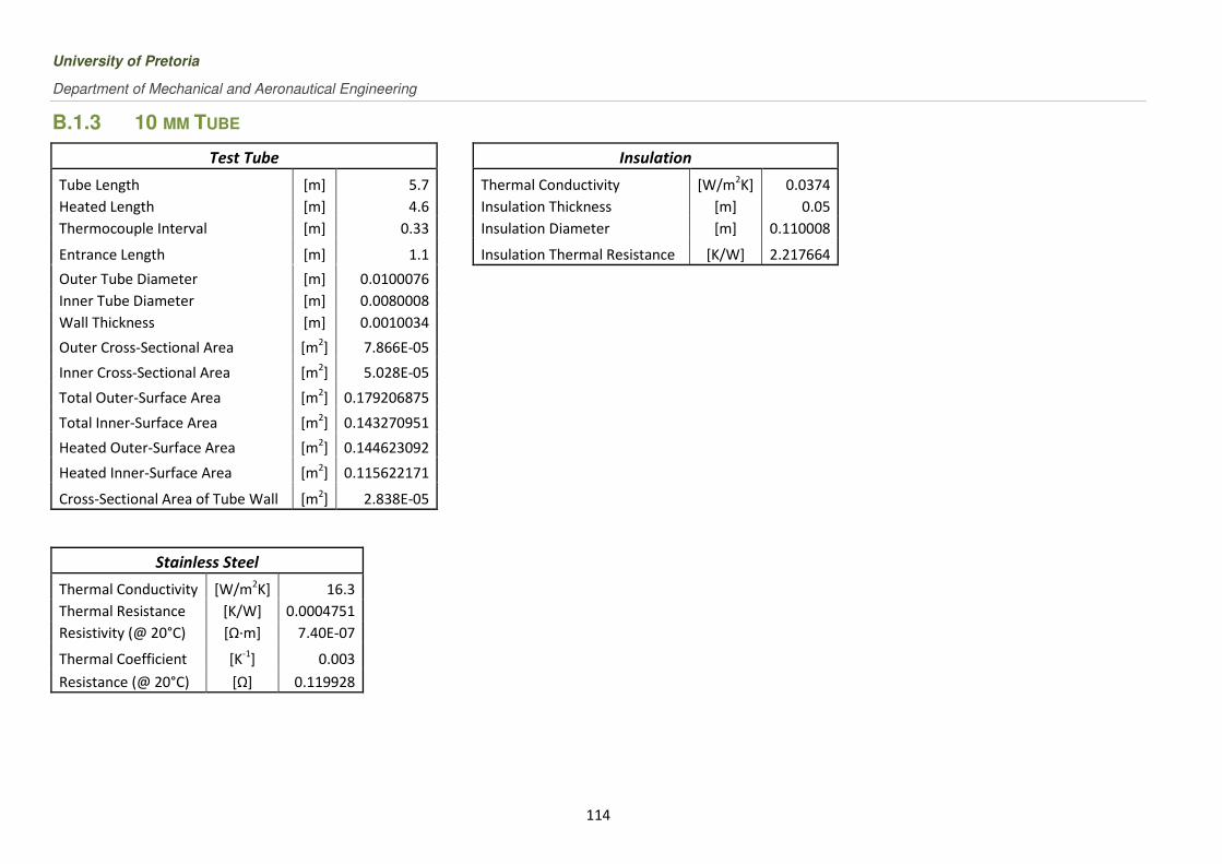
University of Pretoria
Department of Mechanical and Aeronautical Engineering
114
B.1.3 10 MM TUBE
Test Tube Insulation
Tube Length [m] 5.7 Thermal Conductivity [W/m2K] 0.0374
Heated Length [m] 4.6 Insulation Thickness [m] 0.05
Thermocouple Interval [m] 0.33 Insulation Diameter [m] 0.110008
Entrance Length [m] 1.1 Insulation Thermal Resistance [K/W] 2.217664
Outer Tube Diameter [m] 0.0100076
Inner Tube Diameter [m] 0.0080008
Wall Thickness [m] 0.0010034
Outer Cross-Sectional Area [m2] 7.866E-05
Inner Cross-Sectional Area [m2] 5.028E-05
Total Outer-Surface Area [m2] 0.179206875
Total Inner-Surface Area [m2] 0.143270951
Heated Outer-Surface Area [m2] 0.144623092
Heated Inner-Surface Area [m2] 0.115622171
Cross-Sectional Area of Tube Wall [m2] 2.838E-05
Stainless Steel
Thermal Conductivity [W/m2K] 16.3
Thermal Resistance [K/W] 0.0004751
Resistivity (@ 20°C) [Ω·m] 7.40E-07
Thermal Coefficient [K-1] 0.003
Resistance (@ 20°C) [Ω] 0.119928

Analysis of Theoretical Heat Transfer Coefficients for Laminar to Turbulent Flow in Smooth Tubes
Melissa Hallquist
115
Steel Resistance
Thermocouple Position - 1 2 3 4 5 6 7 8 9 10 11 12 13 14 15
Thermocouple Position [m] 1.1 1.43 1.76 2.09 2.42 2.75 3.08 3.41 3.74 4.07 4.4 4.73 5.06 5.39 5.7
Placement [m] 0 0.33 0.66 0.99 1.32 1.65 1.98 2.31 2.64 2.97 3.3 3.63 3.96 4.29 4.6
Resistance (@ 20°C) [Ω] 0 0.009 0.017 0.026 0.034 0.043 0.052 0.060 0.069 0.077 0.086 0.095 0.103 0.112 0.120

University of Pretoria
Department of Mechanical and Aeronautical Engineering
116
B.2 AVERAGE RESULTS
Below is an example of the spreadsheet used to determine the average Nusselt number prior to determining the local values. This spreadsheet was used as an initial
approximation for the local calculations.
DESCRIPTION FIRST DIAPHRAGM
Properties Units 800 900 1000 1100 1200 1300 1400 1500 1600 1700 1800 1900
Inlet Temperature [°C] 22.719 22.601 22.162 21.883 21.616 21.417 21.203 20.906 20.813 20.629 20.350 19.977
Outlet Temperature [°C] 59.005 57.057 49.958 46.687 43.567 42.038 39.595 37.706 36.478 35.222 33.926 32.584
Bulk Temperature [°C] 40.862 39.829 36.060 34.285 32.591 31.728 30.399 29.306 28.646 27.925 27.138 26.281
Average Wall
Temperature [°C] 47.068 45.959 42.017 40.281 38.575 37.713 36.417 35.390 34.668 33.987 33.233 32.372
Inlet Tau - 0.5428 0.5430 0.5436 0.5441 0.5445 0.5448 0.5451 0.5456 0.5457 0.5460 0.5464 0.5470
Inlet Density [kg/m3] 997.559 997.587 997.688 997.751 997.811 997.855 997.902 997.967 997.987 998.026 998.085 998.163
Tau - 0.5147 0.5163 0.5222 0.5249 0.5275 0.5289 0.5309 0.5326 0.5336 0.5347 0.5359 0.5373
Density [kg/m3] 991.838 992.236 993.618 994.230 994.791 995.068 995.481 995.809 996.003 996.209 996.430 996.663
Viscosity [kg/ms] 6.42E-04 6.55E-04 7.04E-04 7.30E-04 7.55E-04 7.69E-04 7.91E-04 8.09E-04 8.21E-04 8.34E-04 8.49E-04 8.65E-04
Thermal conductivity [W/m2K] 0.632 0.630 0.625 0.623 0.621 0.619 0.618 0.616 0.615 0.614 0.613 0.612
Prandtl number - 4.245 4.337 4.699 4.887 5.078 5.180 5.344 5.484 5.572 5.671 5.782 5.906
Thermal expansion [1/K] 3.92E-04 3.84E-04 3.54E-04 3.39E-04 3.25E-04 3.18E-04 3.06E-04 2.96E-04 2.90E-04 2.84E-04 2.76E-04 2.68E-04
Specific Heat [J/kgK] 4178.920 4178.805 4178.590 4178.610 4178.707 4178.787 4178.956 4179.136 4179.265 4179.422 4179.615 4179.852
Mass Flow [kg/s] 0.00261 0.00278 0.00353 0.00396 0.00449 0.00477 0.00536 0.00590 0.00634 0.00682 0.00739 0.00778
Velocity [m/s] 0.0905 0.0963 0.1223 0.1372 0.1554 0.1651 0.1856 0.2042 0.2196 0.2361 0.2558 0.2694
Reynolds Number - 848.390 885.667 1048.001 1135.297 1242.815 1297.577 1418.612 1525.357 1617.583 1711.982 1823.324 1884.633
Corrected Pressure [kPa] 0.2166 0.2434 0.3334 0.4204 0.4905 0.5262 0.6118 0.6776 0.7308 0.7919 0.8667 0.9457
Calibrated Pressure [kPa] 0.2337 0.2608 0.3518 0.4398 0.5107 0.5468 0.6333 0.6998 0.7536 0.8154 0.8910 0.9709

Analysis of Theoretical Heat Transfer Coefficients for Laminar to Turbulent Flow in Smooth Tubes
Melissa Hallquist
117
Friction Factor - 0.0726 0.0716 0.0597 0.0593 0.0537 0.0509 0.0466 0.0425 0.0396 0.0371 0.0345 0.0339
Electrical Resistance [Ω] 0.1842 0.1836 0.1816 0.1807 0.1799 0.1794 0.1788 0.1782 0.1779 0.1775 0.1771 0.1767
Power Dissipation [W] 462.182 461.128 456.251 454.022 451.832 450.724 449.419 447.920 446.994 445.762 445.328 443.513
Heat Transfer [W] 396.294 400.349 410.397 410.804 411.778 411.061 412.033 414.157 415.343 415.941 419.265 410.174
Actual Heat Transfer [W] 429.238 430.738 433.324 432.413 431.805 430.893 430.726 431.038 431.168 430.852 432.297 426.844
Heat Flux [W/m2] 4678.89 4695.25 4723.43 4713.50 4706.87 4696.93 4695.11 4698.52 4699.93 4696.48 4712.23 4652.79
Percentage Error [%] -7.675 -7.055 -5.291 -4.997 -4.638 -4.602 -4.340 -3.916 -3.670 -3.461 -3.014 -3.905
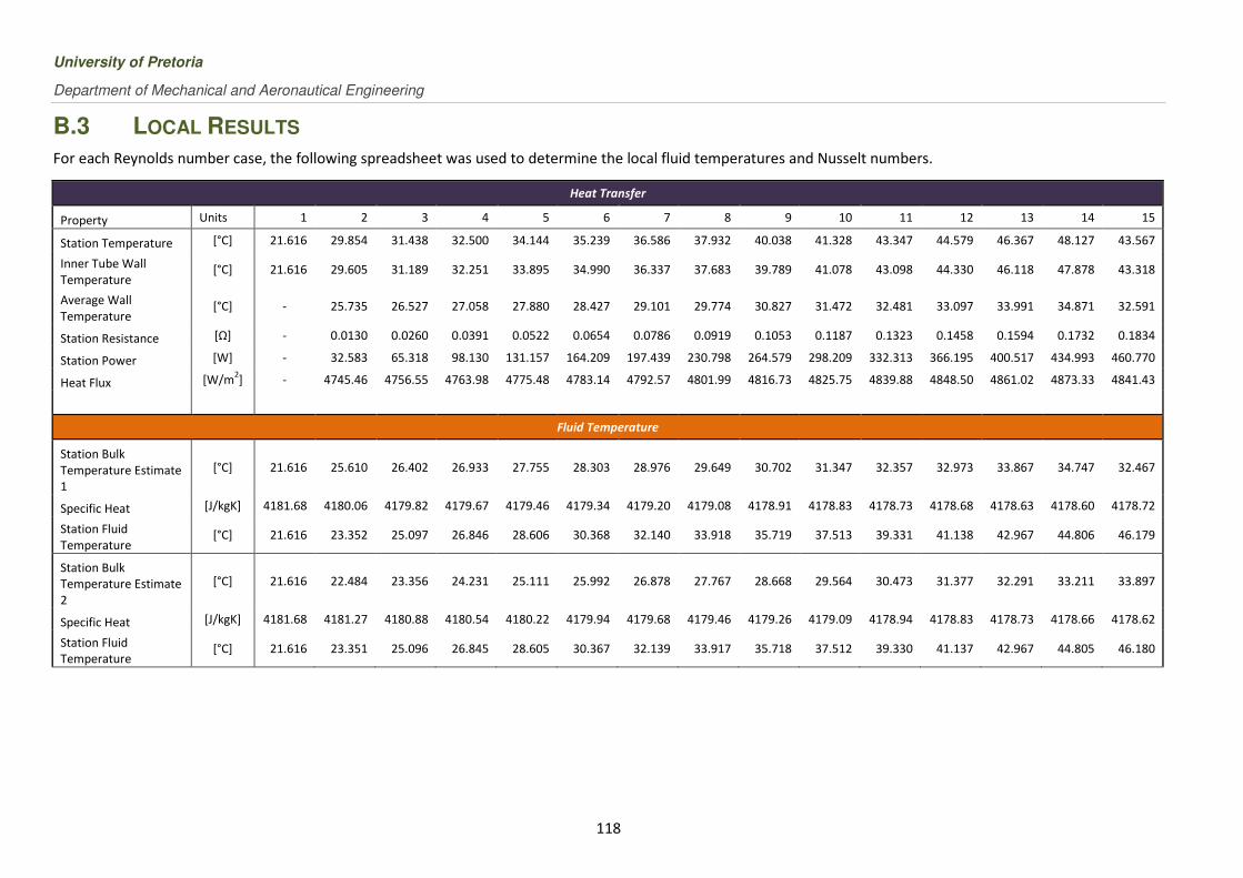
University of Pretoria
Department of Mechanical and Aeronautical Engineering
118
B.3 LOCAL RESULTS
For each Reynolds number case, the following spreadsheet was used to determine the local fluid temperatures and Nusselt numbers.
Heat Transfer
Property Units 1 2 3 4 5 6 7 8 9 10 11 12 13 14 15
Station Temperature [°C] 21.616 29.854 31.438 32.500 34.144 35.239 36.586 37.932 40.038 41.328 43.347 44.579 46.367 48.127 43.567
Inner Tube Wall
Temperature [°C] 21.616 29.605 31.189 32.251 33.895 34.990 36.337 37.683 39.789 41.078 43.098 44.330 46.118 47.878 43.318
Average Wall
Temperature [°C] - 25.735 26.527 27.058 27.880 28.427 29.101 29.774 30.827 31.472 32.481 33.097 33.991 34.871 32.591
Station Resistance [Ω] - 0.0130 0.0260 0.0391 0.0522 0.0654 0.0786 0.0919 0.1053 0.1187 0.1323 0.1458 0.1594 0.1732 0.1834
Station Power [W] - 32.583 65.318 98.130 131.157 164.209 197.439 230.798 264.579 298.209 332.313 366.195 400.517 434.993 460.770
Heat Flux [W/m2] - 4745.46 4756.55 4763.98 4775.48 4783.14 4792.57 4801.99 4816.73 4825.75 4839.88 4848.50 4861.02 4873.33 4841.43
Fluid Temperature
Station Bulk
Temperature Estimate
1
[°C] 21.616 25.610 26.402 26.933 27.755 28.303 28.976 29.649 30.702 31.347 32.357 32.973 33.867 34.747 32.467
Specific Heat [J/kgK] 4181.68 4180.06 4179.82 4179.67 4179.46 4179.34 4179.20 4179.08 4178.91 4178.83 4178.73 4178.68 4178.63 4178.60 4178.72
Station Fluid
Temperature [°C] 21.616 23.352 25.097 26.846 28.606 30.368 32.140 33.918 35.719 37.513 39.331 41.138 42.967 44.806 46.179
Station Bulk
Temperature Estimate
2
[°C] 21.616 22.484 23.356 24.231 25.111 25.992 26.878 27.767 28.668 29.564 30.473 31.377 32.291 33.211 33.897
Specific Heat [J/kgK] 4181.68 4181.27 4180.88 4180.54 4180.22 4179.94 4179.68 4179.46 4179.26 4179.09 4178.94 4178.83 4178.73 4178.66 4178.62
Station Fluid
Temperature [°C] 21.616 23.351 25.096 26.845 28.605 30.367 32.139 33.917 35.718 37.512 39.330 41.137 42.967 44.805 46.180

Analysis of Theoretical Heat Transfer Coefficients for Laminar to Turbulent Flow in Smooth Tubes
Melissa Hallquist
119
Station Bulk Temperature
Estimate 3
[°C] 21.616 22.483 23.356 24.230 25.110 25.991 26.877 27.766 28.667 29.564 30.473 31.376 32.291 33.210 33.898
Specific Heat [J/kgK] 4181.68 4181.27 4180.89 4180.54 4180.22 4179.94 4179.68 4179.46 4179.26 4179.09 4178.95 4178.83 4178.73 4178.66 4178.62
Station Fluid Temperature [°C] 21.616 23.351 25.096 26.845 28.605 30.367 32.139 33.917 35.718 37.512 39.330 41.137 42.967 44.805 46.180
Station Bulk Temperature
Estimate 4
[°C] 21.616 22.483 23.356 24.230 25.110 25.991 26.877 27.766 28.667 29.564 30.473 31.376 32.291 33.210 33.898
Specific Heat [J/kgK] 4181.68 4181.27 4180.89 4180.54 4180.22 4179.94 4179.68 4179.46 4179.26 4179.09 4178.95 4178.83 4178.73 4178.66 4178.62
Station Fluid Temperature [°C] 21.616 23.351 25.096 26.845 28.605 30.367 32.139 33.917 35.718 37.512 39.330 41.137 42.967 44.805 46.180
Station Bulk Temperature
Estimate 5
[°C] 21.616 22.483 23.356 24.230 25.110 25.991 26.877 27.766 28.667 29.564 30.473 31.376 32.291 33.210 33.898
Specific Heat [J/kgK] 4181.68 4181.27 4180.89 4180.54 4180.22 4179.94 4179.68 4179.46 4179.26 4179.09 4178.95 4178.83 4178.73 4178.66 4178.62
Station Fluid Temperature [°C] 21.616 23.351 25.096 26.845 28.605 30.367 32.139 33.917 35.718 37.512 39.330 41.137 42.967 44.805 46.180
Station Bulk Temperature
Estimate 6
[°C] 21.616 22.483 23.356 24.230 25.110 25.991 26.877 27.766 28.667 29.564 30.473 31.376 32.291 33.210 33.898
Specific Heat [J/kgK] 4181.68 4181.27 4180.89 4180.54 4180.22 4179.94 4179.68 4179.46 4179.26 4179.09 4178.95 4178.83 4178.73 4178.66 4178.62
Station Fluid Temperature [°C] 21.616 23.351 25.096 26.845 28.605 30.367 32.139 33.917 35.718 37.512 39.330 41.137 42.967 44.805 46.180
Station Bulk Temperature
Estimate 7
[°C] 21.616 22.483 23.356 24.230 25.110 25.991 26.877 27.766 28.667 29.564 30.473 31.376 32.291 33.210 33.898
Specific Heat [J/kgK] 4181.68 4181.27 4180.89 4180.54 4180.22 4179.94 4179.68 4179.46 4179.26 4179.09 4178.95 4178.83 4178.73 4178.66 4178.62
Station Fluid Temperature [°C] 21.616 23.351 25.096 26.845 28.605 30.367 32.139 33.917 35.718 37.512 39.330 41.137 42.967 44.805 46.180
Station Bulk Temperature
Estimate 8
[°C] 21.616 22.483 23.356 24.230 25.110 25.991 26.877 27.766 28.667 29.564 30.473 31.376 32.291 33.210 33.898
Specific Heat [J/kgK] 4181.68 4181.27 4180.89 4180.54 4180.22 4179.94 4179.68 4179.46 4179.26 4179.09 4178.95 4178.83 4178.73 4178.66 4178.62

University of Pretoria
Department of Mechanical and Aeronautical Engineering
120
Station Fluid Temperature [°C] 21.616 23.351 25.096 26.845 28.605 30.367 32.139 33.917 35.718 37.512 39.330 41.137 42.967 44.805 46.180
Station Bulk Temperature
Estimate 9
[°C] 21.616 22.483 23.356 24.230 25.110 25.991 26.877 27.766 28.667 29.564 30.473 31.376 32.291 33.210 33.898
Specific Heat [J/kgK] 4181.68 4181.27 4180.89 4180.54 4180.22 4179.94 4179.68 4179.46 4179.26 4179.09 4178.95 4178.83 4178.73 4178.66 4178.62
Station Fluid Temperature [°C] 21.616 23.351 25.096 26.845 28.605 30.367 32.139 33.917 35.718 37.512 39.330 41.137 42.967 44.805 46.180
Station Bulk Temperature
Estimate 10
[°C] 21.616 22.483 23.356 24.230 25.110 25.991 26.877 27.766 28.667 29.564 30.473 31.376 32.291 33.210 33.898
Specific Heat [J/kgK] 4181.68 4181.27 4180.89 4180.54 4180.22 4179.94 4179.68 4179.46 4179.26 4179.09 4178.95 4178.83 4178.73 4178.66 4178.62
Station Fluid Temperature [°C] 21.616 23.351 25.096 26.845 28.605 30.367 32.139 33.917 35.718 37.512 39.330 41.137 42.967 44.805 46.180
Fluid Properties
Tau - 0.544 0.542 0.539 0.536 0.534 0.531 0.528 0.525 0.523 0.520 0.517 0.514 0.511 0.509 -
Density [kg/m3] 997.81 997.41 996.97 996.51 996.01 995.49 994.94 994.35 993.74 993.10 992.42 991.73 991.00 990.25 -
Viscosity [kg/ms]
9.64E-
04
9.25E-
04
8.88E-
04
8.54E-
04
8.22E-
04
7.91E-
04
7.62E-
04
7.35E-
04
7.09E-
04
6.85E-
04
6.61E-
04
6.39E-
04
6.18E-
04
5.98E-
04 -
Thermal conductivity [W/m2K] 0.604 0.607 0.610 0.612 0.615 0.618 0.620 0.622 0.625 0.627 0.630 0.632 0.634 0.636 -
Prandtl number - 6.665 6.366 6.086 5.824 5.578 5.348 5.131 4.928 4.735 4.554 4.382 4.221 4.068 3.923 -
Thermal expansion [1/K]
2.23E-
04
2.40E-
04
2.57E-
04
2.74E-
04
2.90E-
04
3.06E-
04
3.21E-
04
3.36E-
04
3.51E-
04
3.65E-
04
3.80E-
04
3.94E-
04
4.07E-
04
4.21E-
04 -
Specific Heat [J/kgK] 4181.68 4180.89 4180.23 4179.69 4179.27 4178.96 4178.75 4178.62 4178.59 4178.63 4178.76 4178.95 4179.22 4179.56 -
Kinematic Viscosity [m
2/s]
9.66E-
07
9.27E-
07
8.91E-
07
8.57E-
07
8.25E-
07
7.95E-
07
7.66E-
07
7.39E-
07
7.13E-
07
6.89E-
07
6.66E-
07
6.44E-
07
6.24E-
07
6.04E-
07 -
Expansion Coefficeint [1/K]
2.23E-
04
2.40E-
04
2.57E-
04
2.74E-
04
2.90E-
04
3.06E-
04
3.21E-
04
3.36E-
04
3.51E-
04
3.65E-
04
3.80E-
04
3.94E-
04
4.07E-
04
4.21E-
04 -
Viscosity at wall
Temperature [kg/ms]
9.64E-
04
8.04E-
04
7.78E-
04
7.61E-
04
7.35E-
04
7.19E-
04
7.00E-
04
6.82E-
04
6.55E-
04
6.40E-
04
6.17E-
04
6.03E-
04
5.84E-
04
5.67E-
04 -
Viscosity Ratio - - 1.150 1.142 1.123 1.117 1.100 1.088 1.077 1.082 1.070 1.072 1.060 1.058 1.055 -
Grashoff Number - - 3833.40 4331.14 4421.25 4945.69 4909.73 5039.59 5084.66 6161.87 6023.04 7079.40 6644.86 7248.18 7789.01 -

Analysis of Theoretical Heat Transfer Coefficients for Laminar to Turbulent Flow in Smooth Tubes
Melissa Hallquist
121
Measured Nusselt Number
Local Heat Transfer
Coefficient [W/m
2K] - 758.89 780.67 881.22 902.77 1034.71 1141.56 1275.19 1183.26 1352.93 1284.50 1518.59 1542.68 1586.08 -
Local Nusselt Number - - 7.59 7.77 8.74 8.91 10.17 11.18 12.44 11.50 13.09 12.39 14.59 14.77 15.13 -
Local Reynolds
Number -
Predicted Nusselt Number
Ghajar (Laminar) - - 7.17 6.15 5.68 5.49 5.28 5.14 5.03 5.12 5.00 5.10 4.95 4.98 5.00 -
Ghajar (Turbulent) - - - - - - - - - - - - - - - -
Ghajar (Transitional) - - - - - - - - - - - - - - - -

University of Pretoria
Department of Mechanical and Aeronautical Engineering
122
B.4 VALIDATED RESULTS
Once the local fluid temperatures had been determined, the average values were re-calculated using the updated values. A sample spreadsheet is included here.
DESCRIPTION FIRST DIAPHRAGM
Property Unit
Symbo
l 800 900 1000 1100 1200 1300 1400 1500 1600
Flow Rate
Mass Flow [kg/s] m 0.0026 0.0028 0.0035 0.0040 0.0045 0.0048 0.0054 0.0059 0.0063
Velocity [m/s] v 0.091 0.096 0.122 0.137 0.155 0.165 0.186 0.204 0.220
Reynolds Number - Re 902.008 935.590
1087.32
7
1172.74
4
1278.06
9
1332.53
3
1452.01
0
1556.26
8
1647.13
4
Pressure
Corrected Pressure [kPa] P 0.217 0.243 0.333 0.420 0.491 0.526 0.612 0.678 0.731
Calibrated Pressure [kPa] P 0.234 0.261 0.352 0.440 0.511 0.547 0.633 0.700 0.754
Friction Factor - f 0.073 0.072 0.060 0.059 0.054 0.051 0.047 0.043 0.040
Temperature
Inlet Temperature [°C] Tfi 22.719 22.601 22.162 21.883 21.616 21.417 21.203 20.906 20.813
Outlet Temperature [°C] Tfo 59.005 57.057 49.958 46.687 43.567 42.038 39.595 37.706 36.478
Bulk Temperature [°C] Tb 44.298 42.857 37.986 35.940 33.984 33.035 31.521 30.258 29.496
Average Wall Temperature [°C] Ts 46.813 45.705 41.765 40.031 38.326 37.464 36.169 35.143 34.422
Fully Developed Fluid Temperature [°C] Tfd 58.513 56.185 48.354 45.134 42.060 40.615 38.246 36.348 35.147
Fully Developed Wall Temperature [°C] T 58.664 56.965 50.838 48.184 45.605 44.369 42.429 40.943 39.937
Bluk Fluid Properties
Inlet Tau - τ 0.543 0.543 0.544 0.544 0.544 0.545 0.545 0.546 0.546

Analysis of Theoretical Heat Transfer Coefficients for Laminar to Turbulent Flow in Smooth Tubes
Melissa Hallquist
123
Inlet Density [kg/m3] ρ 997.559 997.587 997.688 997.751 997.811 997.855 997.902 997.967 997.987
Tau - τ 0.509 0.512 0.519 0.522 0.525 0.527 0.529 0.531 0.532
Density [kg/m3] ρ 990.460 991.048 992.925 993.660 994.332 994.646 995.133 995.524 995.753
Viscosity [kg/ms] μ 6.03E-04 6.19E-04 6.78E-04 7.06E-04 7.34E-04 7.48E-04 7.72E-04 7.93E-04 8.06E-04
Thermal conductivity
[W/m2K
] k 0.636 0.634 0.628 0.625 0.623 0.621 0.619 0.617 0.616
Prandtl number - Pr 3.962 4.077 4.508 4.712 4.921 5.027 5.205 5.362 5.460
Thermal expansion [1/K] β 4.17E-04 4.07E-04 3.69E-04 3.53E-04 3.37E-04 3.29E-04 3.16E-04 3.05E-04 2.98E-04
Specific Heat [J/kgK] Cp
4179.46
2
4179.20
6
4178.65
9
4178.58
9
4178.62
1
4178.67
3
4178.81
0
4178.97
7
4179.10
2
Kinematic Viscosity [m2/s] ν 6.09E-07 6.25E-07 6.83E-07 7.10E-07 7.38E-07 7.52E-07 7.76E-07 7.97E-07 8.09E-07
Grashoff Number - Gr 6207.96 6511.36 6565.04 6278.14 5888.57 5645.19 5349.57 5147.82 4915.85
Raleigh Number - Ra
24597.5
1
26547.2
7
29596.6
3
29580.9
3
28974.9
0
28379.6
7
27845.5
8
27600.4
8
26838.6
2
Viscosity at wall temperature [kg/ms] μ 0.001 0.001 0.001 0.001 0.001 0.001 0.001 0.001 0.001
Viscosity Ratio - μb/μw 1.016 1.018 1.024 1.026 1.027 1.028 1.029 1.031 1.031
Fully Developed Fluid Properties
Inlet Tau - τ 0.543 0.543 0.544 0.544 0.544 0.545 0.545 0.546 0.546
Inlet Density [kg/m3] ρ 997.56 997.59 997.69 997.75 997.81 997.86 997.90 997.97 997.99
Tau - τ 0.487 0.491 0.503 0.508 0.513 0.515 0.519 0.522 0.524
Density [kg/m3] ρ 983.91 985.07 988.73 990.11 991.37 991.93 992.83 993.52 993.94
Viscosity [kg/ms] μ 4.77E-04 4.94E-04 5.62E-04 5.94E-04 6.28E-04 6.45E-04 6.75E-04 7.00E-04 7.17E-04
Thermal conductivity
[W/m2K
] k 0.651 0.649 0.640 0.637 0.633 0.631 0.628 0.626 0.624
Prandtl number - Pr 3.066 3.188 3.666 3.898 4.143 4.267 4.483 4.670 4.795
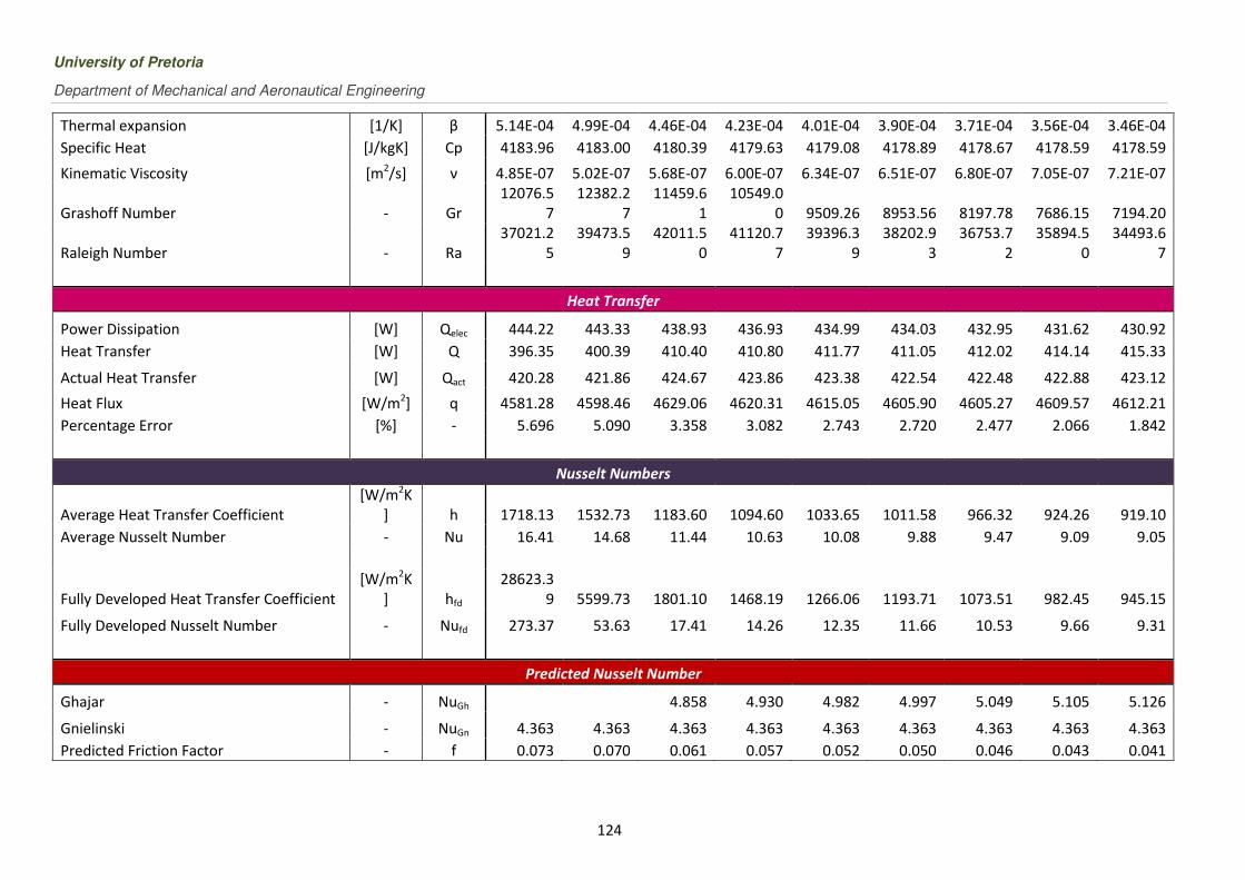
University of Pretoria
Department of Mechanical and Aeronautical Engineering
124
Thermal expansion [1/K] β 5.14E-04 4.99E-04 4.46E-04 4.23E-04 4.01E-04 3.90E-04 3.71E-04 3.56E-04 3.46E-04
Specific Heat [J/kgK] Cp 4183.96 4183.00 4180.39 4179.63 4179.08 4178.89 4178.67 4178.59 4178.59
Kinematic Viscosity [m2/s] ν 4.85E-07 5.02E-07 5.68E-07 6.00E-07 6.34E-07 6.51E-07 6.80E-07 7.05E-07 7.21E-07
Grashoff Number - Gr
12076.5
7
12382.2
7
11459.6
1
10549.0
0 9509.26 8953.56 8197.78 7686.15 7194.20
Raleigh Number - Ra
37021.2
5
39473.5
9
42011.5
0
41120.7
7
39396.3
9
38202.9
3
36753.7
2
35894.5
0
34493.6
7
Heat Transfer
Power Dissipation [W] Qelec 444.22 443.33 438.93 436.93 434.99 434.03 432.95 431.62 430.92
Heat Transfer [W] Q 396.35 400.39 410.40 410.80 411.77 411.05 412.02 414.14 415.33
Actual Heat Transfer [W] Qact 420.28 421.86 424.67 423.86 423.38 422.54 422.48 422.88 423.12
Heat Flux [W/m2] q 4581.28 4598.46 4629.06 4620.31 4615.05 4605.90 4605.27 4609.57 4612.21
Percentage Error [%] - 5.696 5.090 3.358 3.082 2.743 2.720 2.477 2.066 1.842
Nusselt Numbers
Average Heat Transfer Coefficient
[W/m2K
] h 1718.13 1532.73 1183.60 1094.60 1033.65 1011.58 966.32 924.26 919.10
Average Nusselt Number - Nu 16.41 14.68 11.44 10.63 10.08 9.88 9.47 9.09 9.05
Fully Developed Heat Transfer Coefficient
[W/m2K
] hfd
28623.3
9 5599.73 1801.10 1468.19 1266.06 1193.71 1073.51 982.45 945.15
Fully Developed Nusselt Number - Nufd 273.37 53.63 17.41 14.26 12.35 11.66 10.53 9.66 9.31
Predicted Nusselt Number
Ghajar - NuGh 4.858 4.930 4.982 4.997 5.049 5.105 5.126
Gnielinski - NuGn 4.363 4.363 4.363 4.363 4.363 4.363 4.363 4.363 4.363
Predicted Friction Factor - f 0.073 0.070 0.061 0.057 0.052 0.050 0.046 0.043 0.041

Analysis of Theoretical Heat Transfer Coefficients for Laminar to Turbulent Flow in Smooth Tubes
Melissa Hallquist
125
Graphs
Stanton Number - St 4.59E-03 3.85E-03 2.33E-03 1.92E-03 1.60E-03 1.48E-03 1.25E-03 1.09E-03 1.01E-03
j-Factor - j 1.05E-02 8.94E-03 5.76E-03 4.88E-03 4.17E-03 3.89E-03 3.37E-03 2.98E-03 2.79E-03
%